strategic financial management - fröken börs
TRANSCRIPT

Robert Alan Hill
Strategic Financial Management
Download free books at

Download free eBooks at bookboon.com
2
R.A. Hill
Strategic Financial Management

Download free eBooks at bookboon.com
3
Strategic Financial Management1st edition© 2008 R.A. Hill & bookboon.comISBN 978-87-7681-425-0

Download free eBooks at bookboon.com
Click on the ad to read more
Strategic Financial Management
4
Contents
Contents
About the Author 9
Part One: An Introduction 10
1 Finance – An Overview 111.1 Financial Objectives and Shareholder Wealth 111.2 Wealth Creation and Value Added 131.3 The Investment and Finance Decision 141.4 Decision Structures and Corporate Governance 171.5 The Developing Finance Function 181.6 The Principles of Investment 221.7 Perfect Markets and the Separation Theorem 241.8 Summary and Conclusions 281.9 Selected References 29
Kunderna som får dig att växa
”Vad skiljer er från andra revisions- och konsultföretag?” Den frågan får vi ofta. Svaret är enkelt. Vårt kundfokus – dynamiska ägarledda företag. Hos oss arbetar du med spännande entreprenörer vars företag vi hjälper att växa och utvecklas. Det gör ditt arbete varierande, utmanande och lärorikt. Du använder dina teoretiska kunskaper, bygger relationer och får värdefull erfarenhet. Vill du utveckla din egen förmåga? Välkommen till oss på Grant Thornton.
www.grantthornton.se/student Facebook: Grant Thornton Sverige Karriär
–Vad skiljer er från andra företag?
Anja BjörklundAuktoriserad revisor

Download free eBooks at bookboon.com
Click on the ad to read more
Strategic Financial Management
5
Contents
Part Two: The Investment Decision 30
2 Capital Budgeting Under Conditions Of Certainty 312.1 The Role of Capital Budgeting 322.2 Liquidity, Profitability and Present Value 332.3 The Internal Rate of Return (IRR) 392.4 The Inadequacies of IRR and the Case for NPV 402.5 Summary and Conclusions 42
3 Capital Budgeting and the Case for NPV 433.1 Ranking and Acceptance Under IRR and NPV 443.2 The Incremental IRR 463.3 Capital Rationing, Project Divisibility and NPV 463.4 Relevant Cash Flows and Working Capital 473.5 Capital Budgeting and Taxation 493.6 NPV and Purchasing Power Risk 503.7 Summary and Conclusions 53
Revisionsplikten i de små aktiebolagen är slopad och företagen behöver fler duktiga rådgivare.
Auktoriserad Redovisningskonsult – ett framtidsyrke
Erbjudande Förmånligt studerandemedlemskap: Starta din karriär redan nu med SRFs studerandemedlemskap. För endast 250 kr/år får du massor av nyttig bransch-information och ett stort kontaktnät. SRF Redovisning: En samlingsvolym med redovisningens alla lagar, regler och rekommendationer. Ladda ner den gratis på bookboon.com eller bläddra i vår digitala bok på srfredovisning.se.
Besök SRFs studentsida >>
Sveriges Redovisningskonsulters Förbund SRF • srfkonsult.se/framtidsyrket

Download free eBooks at bookboon.com
Click on the ad to read more
Strategic Financial Management
6
Contents
4 The Treatment of Uncertainty 544.1 Dysfunctional Risk Methodologies 554.2 Decision Trees, Sensitivity and Computers 554.3 Mean-Variance Methodology 564.4 Mean-Variance Analyses 584.5 The Mean-Variance Paradox 604.5 Certainty Equivalence and Investor Utility 624.6 Summary and Conclusions 644.7 Reference 64
Part Three: The Finance Decision 65
5 Equity Valuation and the Cost of Capital 665.1 The Capitalisation Concept 675.2 Single-Period Dividend Valuation 685.3 Finite Dividend Valuation 685.4 General Dividend Valuation 695.5 Constant Dividend Valuation 695.6 The Dividend Yield and Corporate Cost of Equity 705.7 Dividend Growth and the Cost of Equity 71
aea.se/blimedlem
@akademikernas på Twitter facebook.com/akademikernas
Akademikernas a-kassaFör alla akademiker. Hela arbetslivet.
Försäkra din lön för 90 kronor
i månaden

Download free eBooks at bookboon.com
Click on the ad to read more
Strategic Financial Management
7
Contents
5.8 Capital Growth and the Cost of Equity 725.9 Growth Estimates and the Cut-Off Rate 735.10 Earnings Valuation and the Cut-Off Rate 755.11 Summary and Conclusions 785.12 Selected References 78
6 Debt Valuation and the Cost of Capital 796.1 Capital Gearing (Leverage): An Introduction 806.2 The Value of Debt Capital and Capital Cost 806.3 The Tax-Deductibility of Debt 846.4 The Impact of Issue Costs 876.5 Summary and Conclusions 89
7 Capital Gearing and the Cost of Capital 917.1 The Weighted Average Cost of Capital (WACC) 927.2 WACC Assumptions 937.3 The Real-World Problems of WACC Estimation 957.4 Summary and Conclusions 1007.5 Selected Reference 100
Vi välkomnar dig till hjärtat av Berlin!Din profil• Flytande i engelska• Vilja att arbeta i ett
internationellt team• Motivation och drivkraft
Vi erbjuder • Praktik och anställning• Flexibla arbetstider • Internationell erfarenhet
www.eon.com/careers

Download free eBooks at bookboon.com
Click on the ad to read more
Strategic Financial Management
8
Contents
Part Four: The Wealth Decision 101
8 Shareholder Wealth and Value Added 1028.1 The Concept of Economic Value Added (EVA) 1038.2 The Concept of Market Value Added (MVA) 1048.3 Profit and Cash Flow 1048.4 EVA and Periodic MVA 1058.5 NPV Maximisation, Value Added and Wealth 1068.6 Summary and Conclusions 1128.7 Selected References 114
Angelica Rydström, medlem sedan 2007FOTO: DAVID FISCHER
08-556 912 00 ⁄ [email protected] ⁄ www.civilekonomerna.se
I studentmedlemskapet ingår en rad nyttiga förmåner som
du kan använda under studietiden. Du får bland
annat karriärmagasinet Civilekonomen tio gånger per
år helt kostnadsfritt. Vi kan ekonomutbildningen
och ekonomers karriär. Fråga oss redan idag!
Det är gratis!
Bli student-medlem!

Download free eBooks at bookboon.com
Strategic Financial Management
9
About the Author
About the AuthorWith an eclectic record of University teaching, research, publication, consultancy and curricula development, underpinned by running a successful business, Alan has been a member of national academic validation bodies and held senior external examinerships and lectureships at both undergraduate and postgraduate level in the UK and abroad.
With increasing demand for global e-learning, his attention is now focussed on the free provision of a financial textbook series, underpinned by a critique of contemporary capital market theory in volatile markets, published by bookboon.com.
To contact Alan, please visit Robert Alan Hill at www.linkedin.com.


Download free eBooks at bookboon.com
Strategic Financial Management
11
Finance – An Overview
1 Finance – An OverviewIntroduction
In a world of geo-political, social and economic uncertainty, strategic financial management is in a process of change, which requires a reassessment of the fundamental assumptions that cut across the traditional boundaries of the subject.
Read on and you will not only appreciate the major components of contemporary finance but also find the subject much more accessible for future reference.
The emphasis throughout is on how strategic financial decisions should be made by management, with reference to classical theory and contemporary research. The mathematics and statistics are simplified wherever possible and supported by numerical activities throughout the text.
1.1 Financial Objectives and Shareholder Wealth
Let us begin with an idealised picture of investors to whom management are ultimately responsible. All the traditional finance literature confirms that investors should be rational, risk-averse individuals who formally analyse one course of action in relation to another for maximum benefit, even under conditions of uncertainty. What should be (rather than what is) we term normative theory. It represents the foundation of modern finance within which:
Investors maximise their wealth by selecting optimum investment and financing opportunities, using financial models that maximise expected returns in absolute terms at minimum risk.
What concerns investors is not simply maximum profit but also the likelihood of it arising: a risk-return trade-off from a portfolio of investments, with which they feel comfortable and which may be unique for each individual. Thus, in a sophisticated mixed market economy where the ownership of a company’s portfolio of physical and monetary assets is divorced from its control, it follows that:
The normative objective of financial management should be:
To implement investment and financing decisions using risk-adjusted wealth maximising criteria, which satisfy the firm’s owners (the shareholders) by placing them all in an equal, optimum financial position.

Download free eBooks at bookboon.com
Strategic Financial Management
12
Finance – An Overview
Of course, we should not underestimate a firm’s financial, fiscal, legal and social responsibilities to all its other stakeholders. These include alternative providers of capital, creditors, employees and customers, through to government and society at large. However, the satisfaction of their objectives should be perceived as a means to an end, namely shareholder wealth maximisation.
As employees, management’s own satisficing behaviour should also be subordinate to those to whom they are ultimately accountable, namely their shareholders, even though empirical evidence and financial scandals have long cast doubt on managerial motivation.
In our ideal world, firms exist to convert inputs of physical and money capital into outputs of goods and services that satisfy consumer demand to generate money profits. Since most economic resources are limited but society’s demand seems unlimited, the corporate management function can be perceived as the future allocation of scarce resources with a view to maximising consumer satisfaction. And because money capital (as opposed to labour) is typically the limiting factor, the strategic problem for financial management is how limited funds are allocated between alternative uses.
The pioneering work of Jenson and Meckling (1976) neatly resolves this dilemma by defining corporate management as agents of the firm’s owners, who are termed the principals. The former are authorised not only to act on the behalf of the latter, but also in their best interests.
Armed with agency theory, you will discover that the function of strategic financial management can be deconstructed into four major components based on the mathematical concept of expected net present value (ENPV) maximisation:
The investment, dividend, financing and portfolio decision.
In our ideal world, each is designed to maximise shareholders’ wealth using the market price of an ordinary share (or common stock to use American parlance) as a performance criterion.
Explained simply, the market price of equity (shares) acts as a control on management’s actions because if shareholders (principals) are dissatisfied with managerial (agency) performance they can always sell part or all of their holding and move funds elsewhere. The law of supply and demand may then kick in, the market value of equity fall and in extreme circumstances management may be replaced and takeover or even bankruptcy may follow. So, to survive and prosper:
The over-arching, normative objective of strategic financial management should be the maximisation of shareholders’ wealth represented by their ownership stake in the enterprise, for which the firm’s current market price per share is a disciplined, universal metric.

Download free eBooks at bookboon.com
Strategic Financial Management
13
Finance – An Overview
1.2 Wealth Creation and Value Added
Modern finance theory regards capital investment as the springboard for wealth creation. Essentially, financial managers maximise stakeholder wealth by generating cash returns that are more favourable than those available elsewhere. In a mature, mixed market economy, they translate this strategic goal into action through the capital market.
Figure 1:1 reveals that companies come into being financed by external funding, which invariably includes debt, as well as equity and perhaps an element of government aid.
If their investment policies satisfy consumer needs, firms should make money profits that at least equal their overall cost of funds, as measured by their investors’ desired rates of return. These will be distributed to the providers of debt capital in the form of interest, with the balance either paid to shareholders as a dividend, or retained by the company to finance future investment to create capital gains.
Either way, managerial ability to sustain or increase the investor returns through a continual search for investment opportunities should then attract further funding from the capital market, so that individual companies grow.
Figure 1.1: The Mixed Market Economy
If firms make money profits that exceed their overall cost of funds (positive ENPV) they create what is termed economic value added (EVA) for their shareholders. EVA provides a financial return to shareholders in excess of their normal return at no expense to other stakeholders. Given an efficient capital market with no barriers to trade, (more of which later) demand for a company’s shares, driven by its EVA, should then rise. The market price of shares will also rise to a higher equilibrium position, thereby creating market value added (MVA) for the mutual benefit of the firm, its owners and prospective investors.
Of course, an old saying is that “the price of shares can fall, as well as rise”, depending on economic performance. Companies engaged in inefficient or irrelevant activities, which produce periodic losses (negative EVA) are gradually starved of finance because of reduced dividends, inadequate retentions and the capital market’s unwillingness to replenish their asset base at lower market prices (negative MVA).

Download free eBooks at bookboon.com
Strategic Financial Management
14
Finance – An Overview
Figure 1.2 distinguishes the “winners” from the “losers” in their drive to add value by summarising in financial terms why some companies fail. These may then fall prey to take-over as share values plummet, or even implode and disappear altogether.
Figure 1:2: Corporate Economic Performance, Winners and Losers.
1.3 The Investment and Finance Decision
On a more optimistic note, we can define successful management policies of wealth maximisation that increase share price, in terms of two distinct but inter-related functions.
Investment policy selects an optimum portfolio of investment opportunities that maximise anticipated net cash inflows (ENPV) at minimum risk.
Finance policy identifies potential fund sources (equity and debt, long or short) required to sustain investment, evaluates the risk-adjusted returns expected by each and then selects the optimum mix that will minimise their overall weighted average cost of capital (WACC).
The two functions are interrelated because the financial returns required by a company’s capital providers must be compared to its business returns from investment proposals to establish whether they should be accepted.
And while investment decisions obviously precede finance decisions (without the former we don’t need the latter) what ultimately concerns the firm is not only the profitability of investment but also whether it satisfies the capital market’s financial expectations.

Download free eBooks at bookboon.com
Click on the ad to read more
Strategic Financial Management
15
Finance – An Overview
Strategic managerial investment and finance functions are therefore inter-related via a company’s weighted, average cost of capital (WACC).
From a financial perspective, it represents the overall costs incurred in the acquisition of funds. A complex concept, it embraces explicit interest on borrowings or dividends paid to shareholders. However, companies also finance their operations by utilising funds from a variety of sources, both long and short term, at an implicit or opportunity cost. Such funds include trade credit granted by suppliers, deferred taxation, as well as retained earnings, without which companies would presumably have to raise funds elsewhere. In addition, there are implicit costs associated with depreciation and other non-cash expenses. These too, represent retentions that are available for reinvestment.
Imagine yourself working with some of the sharpest and most creative brains in the transport and infrastructure industry, developing sustainable transport solutions that will change the future of society.
Imagine yourself working in a company that really believes that people are its driving force, fostering a culture of energy, passion and respect for the individual.
Imagine yourself working for the Volvo Group, a global leader in sustainable transport solutions with about 110,000 employees, production in 18 countries and sales in about 190 countries. A place where your voice is heard and your ideas matter.
Together we move the world.
www.volvogroup.com/career
SHAPINGANOTHER FUTURE

Download free eBooks at bookboon.com
Strategic Financial Management
16
Finance – An Overview
In terms of the corporate investment decision, a firm’s WACC represents the overall cut-off rate that justifies the financial decision to acquire funding for an investment proposal (as we shall discover, a zero NPV).
In an ideal world of wealth maximisation, it follows that if corporate cash profits exceed overall capital costs (WACC) then NPV will be positive, producing a positive EVA. Thus:
- If management wish to increase shareholder wealth, using share price (MVA) as a vehicle, then it must create positive EVA as the driver.
- Negative EVA is only acceptable in the short term. - If share price is to rise long term, then a company should not invest funds
from any source unless the marginal yield on new investment at least equals the rate of return that the provider of capital can earn elsewhere on comparable investments of equivalent risk.
Figure 1:3 overleaf, charts the strategic objectives of financial management relative to the investment and finance decisions that enhance corporate wealth and share price.
Figure 1.3: Strategic Financial Management

Download free eBooks at bookboon.com
Strategic Financial Management
17
Finance – An Overview
1.4 Decision Structures and Corporate Governance
We can summarise the normative objectives of strategic financial management as follows:
The determination of a maximum inflow of cash profit and hence corporate value, subject to acceptable levels of risk associated with investment opportunities, having acquired capital efficiently at minimum cost.
Investment and financial decisions can also be subdivided into two broad categories; longer term (strategic or tactical) and short-term (operational). The former may be unique, typically involving significant fixed asset expenditure but uncertain future gains. Without sophisticated periodic forecasts of required outlays and associated returns, which incorporate time value of money techniques, such as ENPV and an allowance for risk, the subsequent penalty for error can be severe; in the extreme, corporate death.
Conversely, operational decisions (the domain of working capital management) tend to be repetitious, or infinitely divisible, so much so that funds may be acquired piecemeal. Costs and returns are usually quantifiable from existing data with any weakness in forecasting easily remedied. The decision itself may not be irreversible.
However, irrespective of the time horizon, the investment and financial decision process should always involve:
- The continual search for investment opportunities. - The selection of the most profitable opportunities, in absolute terms. - The determination of the optimal mix of internal and external funds required to finance
those opportunities. - The establishment of a system of financial controls governing the acquisition and disposition
of funds. - The analysis of financial results as a guide to future decision-making.
Needless to say, none of these functions are independent of the other. All occupy a pivotal position in the decision making process and naturally require co-ordination at the highest level. And this is where corporate governance comes into play.
We mentioned earlier that empirical observations of agency theory reveal that management might act irresponsibly, or have different objectives. These may be sub-optimal relative to shareholders wealth maximisation, particularly if management behaviour is not monitored, or they receive inappropriate incentives (see Ang, Rebel and Lin, 2000).

Download free eBooks at bookboon.com
Strategic Financial Management
18
Finance – An Overview
To counteract corporate mis-governance a system is required whereby firms are monitored and controlled. Now termed corporate governance, it should embrace the relationships between the ordinary shareholders, Board of Directors and senior management, including the Chief Executive Officer (CEO).
In large public companies where goal congruence is a particular problem (think Enron, or the 2007–8 sub-prime mortgage and banking crisis) the Board of Directors (who are elected by the shareholders) and operate at the interface between shareholders and management is widely regarded as the key to effective corporate governance. In our ideal world, they should not only determine ethical company policies but should also act as a constraint on any managerial actions that might conflict with shareholders interests. For an international review of the theoretical and empirical research on the subject see the Journal of Financial and Quantitative Analysis 38 (2003).
1.5 The Developing Finance Function
We began our introduction with a portrait of rational, risk averse investors and the corporate environment within which they operate. However, a broader picture of the role of modern financial management can be painted through an appreciation of its historical development. Chronologically, six main features can be discerned:
- Traditional - Managerial - Economic - Systematic - Behavioural - Post Modern
Traditional thinking predates the Second World War. Positive in approach, which means a concern with what is (rather than normative and what should be), the discipline was Balance Sheet dominated. Financial management was presented in the literature as merely a classification and description of long term sources of funds with instructions on how to acquire them and at what cost. Any emphasis upon the use of funds was restricted to fixed asset investment using the established techniques of payback and accounting rate of return (ARR) with their emphasis upon liquidity and profitability respectively.

Download free eBooks at bookboon.com
Click on the ad to read more
Strategic Financial Management
19
Finance – An Overview
Managerial techniques developed during the 1940s from an American awareness that numerous wide-ranging military, logistical techniques (mathematical, statistical and behavioural) could successfully be applied to short term financial management; notably inventory control. The traditional idea that long term finance should be used for long term investment was also reinforced by the notion that wherever possible current assets should be financed by current liabilities, with an emphasis on credit worthiness measured by the working capital ratio. Unfortunately, like financial accounting to which it looked for inspiration; financial management (strategic, or otherwise) still lacked any theoretical objective or model of investment behaviour.
Economic theory, which was normative in approach, came to the rescue. Spurred on by post-war recovery and the advent of computing, throughout the 1950s an increasing number of academics (again mostly American) began to refine and to apply the work of earlier economists and statisticians on discounted revenue theory to the corporate environment.
The initial contribution of the financial literature to financial practice was the development of capital budgeting models utilising time value of money techniques based on the discounted cash flow concept (DCF). From this arose academic suggestions that if management are to satisfy the objectives of corporate stakeholders (including the shareholders to whom they are ultimately responsible) then perhaps they should maximise the net inflow of cash funds at minimum cost.

Download free eBooks at bookboon.com
Strategic Financial Management
20
Finance – An Overview
By the 1960s, (the golden era of finance) an econometric emphasis upon investor and shareholder welfare produced competing theories of share price maximisation, optimal capital structure and the pricing of equity and debt in capital markets using partial equilibrium analysis, all of which were subjected to exhaustive empirical research.
Throughout the 1970s, rigorous analytical, linear techniques based upon investor rationality, the random behaviour of economic variables and stock market efficiency overtook the traditional approach. The managerial concept of working capital with its emphasis on solvency and liquidity at the expense of future profitability was also subject to economic analysis. As a consequence, there emerged an academic consensus that:
The normative objective of finance is represented by the maximisation of shareholders’ welfare measured by share price, achievable through the maximisation of the expected net present value (ENPV) of all a company’s prospective capital investments.
Since the 1970s, however, there has also been a significant awareness that the ebb and flow of finance through investor portfolios, the corporate environment and global capital markets cannot be analysed in a technical vacuum characterised by mathematics, statistics and equilibrium analysis. Efficient financial management, or so the argument goes, must relate to all the other functions within the system that it serves. Only then will it optimise the benefits that accrue to the system as a whole.
Systematic proponents, whose origins lie in management science, still emphasise the financial decisions-maker’s responsibility for the maximisation of corporate value. However, their most recent work focuses upon the interaction of financial decisions with those of other business functions within imperfect markets. More specifically, it questions the economist’s assumptions that investors are rational, returns are random and stock markets are efficient. All of which depend upon the instantaneous recognition of interrelated flows of information and non-financial resources, as well as cash, throughout the system.
Behavioural scientists, particularly communications theorists, have developed this approach further by suggesting that perhaps we can’t maximise anything. They analyse the reaction of individuals, firms and stock market participants to the impersonal elements: cash, information and resources. Emphasis is placed upon the role of competing goals, expectations and choice (some quantitative, others qualitative) in the decision process.
Post-Modern research has really taken off since the millennium and the dot.com-techno crisis, spurred on by global financial meltdown and recession. Whilst still in its infancy, its purpose seems to provide a better understanding of how adaptive human behaviour, which may not be rational or risk-averse, determines investment, corporate and stock market performance in today’s volatile, chaotic world and vice versa.

Download free eBooks at bookboon.com
Click on the ad to read more
Strategic Financial Management
21
Finance – An Overview
So, what of the future?
Obviously, there will be new approaches to financial management whose success will be measured by the extent to which each satisfies its stated objectives. The problem today is that history tells us that every school of academic thought (from traditionalists through to post-modernists) has failed to convince practising financial managers that their approach is always better than another. A particular difficulty is that if their objectives are too broad they are dismissed as self evident. And if they are too specific, they fail to gain general acceptance.
Perhaps the best way foreword is a trade-off between flexibility and uniformity, whereby none of the chronological developments outlined above should be regarded as mutually exclusive. As we shall discover, a particular approach may be more appropriate for a particular decision but overall each has a role to play in contemporary financial management. So, why not focus on how the various chronological elements can be combined to provide a more eclectic (comprehensive) approach to the decision process? Moreover, an historical perspective of the developments and changes that have occurred in finance can also provide fresh insights into long established practice.
STUDY FOR YOUR MASTER’S DEGREE
Chalmers University of Technology conducts research and education in engineer-ing and natural sciences, architecture, technology-related mathematical sciences and nautical sciences. Behind all that Chalmers accomplishes, the aim persists for contributing to a sustainable future – both nationally and globally.
Visit us on Chalmers.se or Next Stop Chalmers on facebook.

Download free eBooks at bookboon.com
Strategic Financial Management
22
Finance – An Overview
As an example, consider investors who use traditional published accounting data such as dividend per share without any reference to economic values to establish a company’s performance. In one respect, their approach can be defended. As we shall see, evidence from statistical studies of share price suggests that increased dividends per share are used by companies to convey positive information concerning future profit and value. But what if the dividend signal contained in the accounts is designed by management to mislead (again think Enron)?
As behaviourists will tell you, irrespective of whether a positive signal is false, if a sufficient number of shareholders and potential investors believe it and purchase shares, then the demand for equity and hence price will rise. Systematically, the firm’s total market capitalisation of equity will follow suit.
Post-modernists will also point out that irrespective of whether management wish to maximise wealth, stock market participants combine periodically to create “crowd behaviour” and market sentiment without reference to any rational expectations based on actual trading fundamentals such as “real” profitability and asset values.
1.6 The Principles of Investment
The previous section illustrates that modern financial management (strategic or otherwise) raises more questions than it can possibly answer. In fairness, theories of finance have developed at an increasing rate over the past fifty years. Unfortunately, unforeseen events always seem to overtake them (for example, the October 1987 crash, the dot.com fiasco of 2000, the aftermath of 7/11, the 2007 sub-prime mortgage crisis and now the consequences of the 2008 financial meltdown).
To many analysts, current financial models also appear more abstract than ever. They attract legitimate criticism concerning their real world applicability in today’s uncertain, global capital market, characterised by geo-political instability, rising oil and commodity prices and the threat of economic recession. Moreover, post-modernists, who take a non-linear view of society and dispense with the assumption that we can maximise anything (long or short) with their talk of speculative bubbles, catastrophe theory and market incoherence, have failed to develop comprehensive alternative models of investment behaviour.
Much work remains to be done. So, in the meantime, let us see what the “old finance” still has to offer today’s investment community and the “new theorists” by adopting a historical perspective and returning to the fundamental principles of investment and shareholder wealth maximisation, a number of which you may be familiar with.

Download free eBooks at bookboon.com
Strategic Financial Management
23
Finance – An Overview
We have observed broad academic agreement that if resources are to be allocated efficiently, the objective of strategic financial management should be:
- To maximise the wealth of the shareholders’ stake in the enterprise.
Companies are assumed to raise funds from their shareholders, or borrow more cheaply from third parties (creditors) to invest in capital projects that generate maximum financial benefit for all.
A capital project is defined as an asset investment that generates a stream of receipts and payments that define the total cash flows of the project. Any immediate payment by a firm for assets is called an initial cash outflow, and future receipts and payments are termed future cash inflows and future cash outflows, respectively.
As we shall discover, wealth maximisation criteria based on expected net present value (ENPV) using a discount rate rather than an internal rate of return (IRR), can then reveal that when fixed and current assets are used efficiently by management:
If ENPV is positive, a project’s anticipated future net cash inflows should enable a firm to repay cheap contractual loans with accumulated interest and provide a higher return to shareholders. This return can take the form of either current dividends, or future capital gains, based on managerial decisions to distribute or retain earnings for reinvestment.
However, this raises a number of questions, even if initial issues of cheap debt capital increase shareholder earnings per share (EPS).
- Do the contractual obligations of larger interest payments associated with more borrowing (and the possibility of higher interest rates to compensate new investors) threaten shareholders returns?
- In the presence of this financial risk associated with increased borrowing (termed gearing or leverage) do rational, risk-averse shareholders prefer current dividend income to future capital gains financed by the retention of their profit?
- Or, irrespective of leverage, are dividends and earnings regarded as perfect economic substitutes in the minds of shareholders?
Explained simply, shareholders are being denied the opportunity to enjoy current dividends if new capital projects are accepted. Of course, they might reap a future capital gain. And in the interim, individual shareholders can also sell part or all of their holdings, or borrow at an appropriate (market) rate of interest to finance their preferences for consumption, or investment in other firms.
But what if a reduction in today’s dividend is not matched by the profitability of management’s future investment opportunities?

Download free eBooks at bookboon.com
Click on the ad to read more
Strategic Financial Management
24
Finance – An Overview
To be consistent with our overall objective of shareholder wealth maximisation, another fundamental principle of investment is that:
Management’s minimum rate of return on incremental projects financed by retained earnings should represent the rate of return that shareholders can expect to earn on comparable investments elsewhere.
Otherwise, corporate wealth will diminish and once this information is signalled to the outside world via an efficient capital market, share price may follow suit.
1.7 Perfect Markets and the Separation Theorem
Since a company’s retained profits for new capital projects represent alternative consumption and investment opportunities foregone by its shareholders, the corporate cut-off rate for investment is termed the opportunity cost of capital. And:
If management vet projects using the shareholders’ opportunity cost of capital as a cut-off rate for investment:
- It should be irrelevant whether future cash flows paid as dividends, or retained for reinvestment, match the consumption preferences of shareholders at any point in time.
- As a consequence, dividends and retentions are perfect substitutes and dividend policy is irrelevant.

Download free eBooks at bookboon.com
Strategic Financial Management
25
Finance – An Overview
Remember, however, that we have assumed shareholders can always sell shares, borrow (or lend) at the market rate of interest, in order to transfer cash from one period to another to satisfy their needs. But for this to work implies that there are no barriers to trade. So, we must also assume that these transactions occur in a perfect capital market if wealth is to be maximised.
Perfect markets, are the bedrock of traditional finance theory that exhibit the following characteristics:
- Large numbers of individuals and companies, none of whom is large enough to distort market prices or interest rates by their own action, (i.e. perfect competition).
- All market participants are free to borrow or lend (invest), or to buy and sell shares. - There are no material transaction costs, other than the prevailing market rate of
interest, to prevent these actions. - All investors have free access to financial information relating to a firm’s projects. - All investors can invest in other companies of equivalent relative risk, in order to
earn their required rare of return. - The tax system is neutral.
Of course, the real world validity of each assumption has long been criticised based on empirical research. For example, not all investors are risk-averse or behave rationally, (why play national lotteries, invest in techno shares, or the sub-prime market?). Share trading also entails costs and tax systems are rarely neutral.
But the relevant question is not whether these assumptions are observable phenomena but do they contribute to our understanding of the capital market?
According to seminal twentieth century research by two Nobel Prize winners for Economics (Franco Modigliani and Merton Miller: 1958 and 1961), of course they do.
The assumptions of a perfect capital market (like the assumptions of perfect competition in economics) provide a sturdy theoretical framework based on logical reasoning for the derivation of more sophisticated applied investment and financial decisions.
Perfect markets underpin our understanding of the corporate wealth maximisation process, irrespective of a firm’s distribution policy, which may include interest on debt, as well as the returns to equity (dividends or capital gains).
Only then, so the argument goes, can we relax each assumption, for example tax neutrality (see Miller 1977), to gauge their differential effects on the real world. What economists term partial equilibrium analysis.

Download free eBooks at bookboon.com
Strategic Financial Management
26
Finance – An Overview
To prove the case for normative theory and the insight that logical reasoning can provide into contemporary managerial investment and financing decisions, we can move back in time even before the traditionalists to the first economic formulation of the impact of perfect market assumptions upon the firm and its shareholders’ wealth.
The Separation Theorem, based upon the pioneering work of Irving Fisher (1930) is quite emphatic concerning the irrelevance of dividend policy.
When a company values capital projects (the managerial investment decision) it does not need to know the expected future spending or consumption patterns of the shareholder clientele (the managerial financing decision).
According to Fisher, once a firm has issued shares and received their proceeds, it is neither directly involved with their subsequent transaction on the capital market, nor the price at which they are traded. This is a matter of negotiation between current shareholders and prospective investors.
So, how can management pursue policies that perpetually satisfy shareholder wealth?
Fisherian Analysis illustrates that in perfect capital markets where ownership is divorced from control, dividend distributions should be an irrelevance.
The corporate investment decision is determined by the market rate of interest, which is separate from an individual shareholder’s preference for consumption.
So finally, let us illustrate the dividend irrelevancy hypothesis and review our introduction to strategic financial management by demonstrating the contribution of Fisher’s theorem to the maximisation of shareholders’ welfare with a simple numerical example.

Download free eBooks at bookboon.com
Click on the ad to read more
Strategic Financial Management
27
Finance – An Overview
Review Activity
A firm is considering two mutually exclusive capital projects of equivalent risk, financed by the retention of current dividends. Each costs £500,000 and their future returns all occur at the end of the first year.
Project A will yield a 15 per cent annual return, generating a cash inflow of £575,000, whereas Project B will earn a 12 per cent return, producing a cash inflow of £560,000.
All individuals and firms can borrow or lend at the prevailing market rate of interest, which is 14 per cent per annum.
Management’s investment decision would appear self-evident.
- If the firm’s total shareholder clientele were to lend £500,000 elsewhere at the 14 per cent market rate of interest, this would only compound to £570,000 by the end of the year. – It is financially more attractive for the firm to retain £500,000 and accumulate £575,000 on the shareholders’ behalf by investing in Project A, since they would have £5,000 more to spend at the year end.
- Conversely, no one benefits if the firm invests in Project B, whose value grows to only £560,000 by the end of the year. Management should pay the dividend.
But suppose that part of the company’s clientele is motivated by a policy of distribution. They need a dividend to spend their proportion of the £500,000 immediately, rather than allow the firm to invest this sum on their behalf.
Armed with this information, should management still proceed with Project A?
We combine BPO, cloud and infrastructure. A formation that can help your career soar.To find out more, visit accenture.cz/career or send your CV to our e-mail [email protected].

Download free eBooks at bookboon.com
Strategic Financial Management
28
Finance – An Overview
1.8 Summary and Conclusions
Based on economic wealth maximisation criteria, corporate financial decisions should always be subordinate to investment decisions, with dividend policy used only as a means of returning surplus funds to shareholders.
To prove the point, our review activity reveals that shareholder funds will be misallocated if management reject Project A and pay a dividend.
For example, as a shareholder with a one per cent stake in the company, who prefers to spend now, you can always borrow £5,000 for a year at the market rate of interest (14 per cent).
By the end of the year, one per cent of the returns from Project A will be worth £5,750. This will more than cover your repayment of £5,000 capital and £700 interest on borrowed funds.
Alternatively, if you prefer saving, rather than lend elsewhere at 14 per cent, it is still preferable to waive the dividend and let the firm invest in Project A because it earns a superior return.
In our Fisherian world of perfect markets, the correct investment decision for wealth maximising firms is to appraise projects on the basis of their shareholders’ opportunity cost of capital.
Endorsed by subsequent academics and global financial consultants, from Hirshliefer (1958) to Stern-Stewart today:
- Projects should only be accepted if their post-tax returns at least equal the returns that shareholders can earn on an investment of equivalent risk elsewhere.
- Projects that earn a return less than this opportunity rate should be rejected. - Project yields that either equal or exceed their opportunity rate can either be distributed or
retained. - The final consumption (spending) decisions of individual shareholders are determined
independently by their personal preferences, since they can borrow or lend to alter their spending patterns accordingly.
From a financial management perspective, dividend distribution policies are an irrelevance, (what academics term a passive residual) in the determination of corporate value and wealth
So, now that we have separated the individual’s consumption decision from the corporate investment decision, let us explore the contemporary world of finance, the various functions of strategic financial management and their analytical models in more detail.
Download free eBooks at bookboon.com
Strategic Financial Management
29
Finance – An Overview
1.9 Selected References
Jensen, M.C. and Meckling, W.H., “Theory of the Firm: Managerial Behaviour, Agency Costs and Ownership Structure”, Journal of Financial Economics, 3, October 1976.
Ang, J.S., Rebel, A. Cole and Lin J.W., “Agency Costs and Ownership Strus3cture” Journal of Finance, 55, February 2000.
Special Issue on International Corporate Governance, (ten articles), Journal of Financial Quantitative Analysis, 38, March 2003.
Miller, M.H. and Modigliani, F., “Dividend policy, growth and the valuation of shares”, The Journal of Business of the University of Chicago, Vol. XXXIV, No. 4 October 1961.
Modigliani, F. and Miller, M.H., “The cost of capital, corporation finance and the theory of investment”, American Economic Review, Vol. XLVIII, No. 3, June 1958.
Miller, M.H., “Debt and Taxes”, The Journal of Finance, Vol. 32, No. 2, May 1977.
Fisher, I., The Theory of Interest, Macmillan (New York), 1930.
Hirshliefer, J.,” On the Theory of Optimal Investment Decisions”, Journal of Political Economy, August 1958.
Stern, J and Stewart, G.B. at www. sternstewart.com.

Download free eBooks at bookboon.com
Strategic Financial Management
31
Capital Budgeting Under Conditions Of Certainty
2 Capital Budgeting Under Conditions Of Certainty
Introduction
The decision to invest is the mainspring of financial management. A project’s acceptance should produce future returns that maximise corporate value at minimum cost to the company.
We shall therefore begin with an explanation of capital budgeting decisions and two common investment methods; payback (PB) and the accounting rate of return (ARR).
Given the failure of both PB and ARR to measure the extent to which the utility of money today is greater or less than money received in the future, we shall then focus upon the internal rate of return (IRR) and net present value (NPV) techniques. Their methodologies incorporate the time value of money by employing discounted cash flow analysis based on the concept of compound interest and a firm’s overall cut-off rate for investment.
For speed of exposition, a mathematical derivation of an appropriate cut-off rate (measured by a company’s weighted average cost of capital, WACC, explained in Part One) will be taken as given until Chapter Three of the follow up SFM text. For the moment, all you need to remember is that in a mixed market economy firms raise funds from various providers of capital who expect an appropriate return from efficient asset investment. And given the assumptions of a perfect capital market with no barriers to trade (also explained in Part One) managerial investment decisions can be separated from shareholder preferences for consumption or investment without compromising wealth maximisation, providing all projects are valued on the basis of their opportunity cost of capital.
As we shall discover, if the firm’s cut-off rate for investment corresponds to this opportunity cost, which represents the return that shareholders can earn elsewhere on similar investments of comparable risk:
Projects that generate a return (IRR) greater than their opportunity cost of capital will have a positive NPV and should be accepted, whereas projects with an inferior IRR (negative NPV) should be rejected.

Download free eBooks at bookboon.com
Click on the ad to read more
Strategic Financial Management
32
Capital Budgeting Under Conditions Of Certainty
2.1 The Role of Capital Budgeting
The financial term capital is broad in scope. It is applied to non-human resources, physical or monetary, short or long. Similarly, budgeting takes many forms but invariably comprises the detailed, quantified planning of a scarce resource for commercial benefit. It implies a choice between alternatives. Thus, a combination of the two terms defines investment and financing decisions which relate to capital assets which are designed to increase corporate profitability and hence value.
To simplify matters, academics and practitioners categorise investment and financing decisions into long-term (strategic) medium (tactical) and short (operational). The latter define working capital management, which represents a firm’s total investment in current assets, (stocks, debtors and cash), irrespective of their financing source. It is supposed to lubricate the wheels of fixed asset investment once it is up and running. Tactics may then change the route. However, capital budgeting proper, by which we mean fixed asset formation, defines the engine that drives the firm forward characterised by three distinguishing features:
Longer term investment; larger financial outlay; greater uncertainty.
Combined with inflation and changing economic conditions, uncertainty complicates any investment decision. We shall therefore defer its effects until Chapter Four having reviewed the basic capital budgeting models in its absence.

Download free eBooks at bookboon.com
Strategic Financial Management
33
Capital Budgeting Under Conditions Of Certainty
With regard to a strategic classification of projects we can identify:
- Diversification defined in terms of new products, services, markets and core technologies which do not compromise long-term profits.
- Expansion of existing activities based on a comparison of long-run returns which stem from increased profitable volume.
- Improvement designed to produce additional revenue or cost savings from existing operations by investing in new or alternative technology.
- Buy or lease based on long-term profitability in relation to alternative financing schemes. - Replacement intended to maintain the firm’s existing operating capability intact, without
necessarily applying the test of profitability.
2.2 Liquidity, Profitability and Present Value
Within the context of capital budgeting, money capital rather than labour or material is usually the scarce resource. In the presence of what is termed capital rationing projects must be ranked in terms of their net benefits compared to the costs of investment. Even if funds are plentiful, the actual projects may be mutually exclusive. The acceptance of one precludes others, an obvious example being the most profitable use of a single piece of land. To assess investment decisions, the following methodologies are commonly used:
Payback; Accounting Rate of Return); Present Value (based on the time value of money).
Payback (PB) is the time required for a stream of cash flows to cover an investment’s cost. The project criterion is liquidity: the sooner the better because of less uncertainty regarding its worth. Assuming annual cash flows are constant, the basic PB formula is given in years by:
(1) PB = I0/Ct
PB = payback periodI0 = capital investment at time period 0Ct = constant net annual cash inflow defined by t = 1
Management’s objective is to accept projects that satisfy their preferred, predetermined PB.
Download free eBooks at bookboon.com
Strategic Financial Management
34
Capital Budgeting Under Conditions Of Certainty
Activity 1
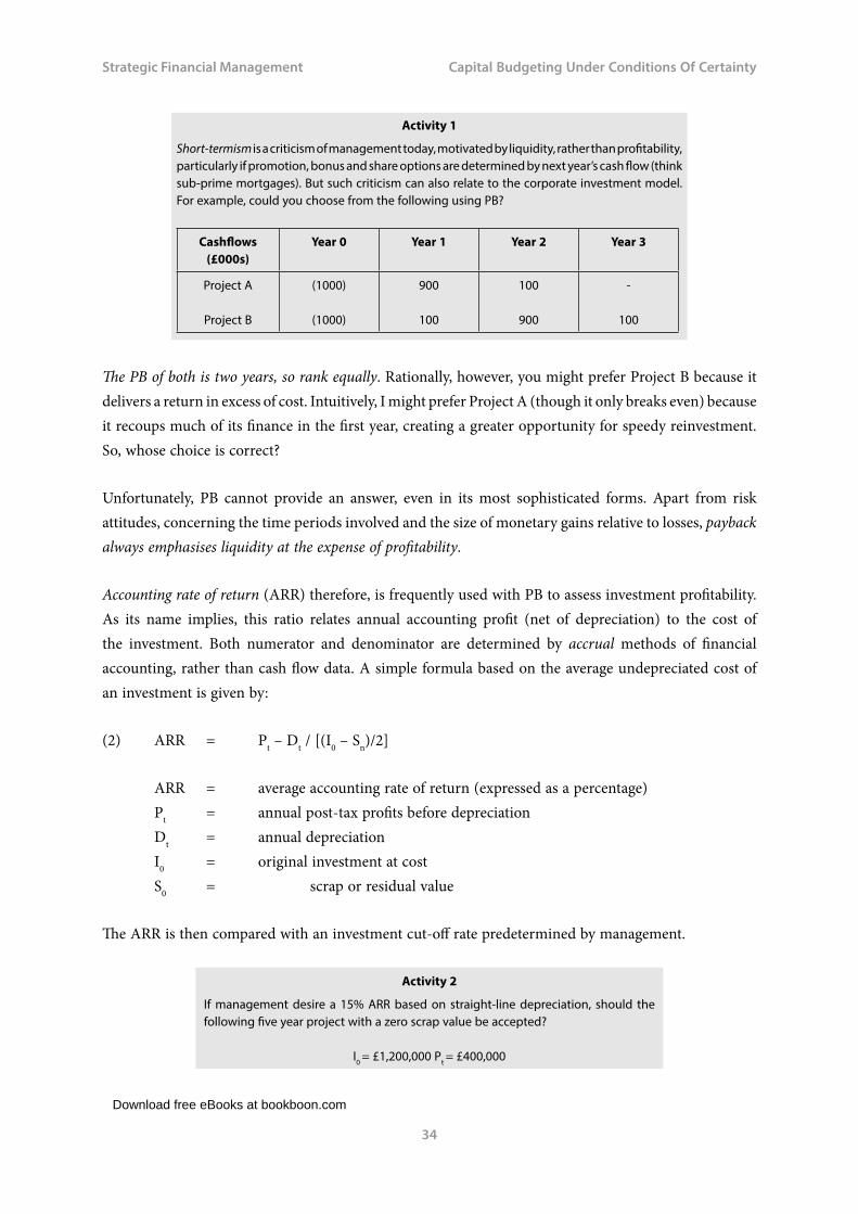
Short-termism is a criticism of management today, motivated by liquidity, rather than profitability, particularly if promotion, bonus and share options are determined by next year’s cash flow (think sub-prime mortgages). But such criticism can also relate to the corporate investment model. For example, could you choose from the following using PB?
Cashflows (£000s)
Year 0 Year 1 Year 2 Year 3
Project A
Project B
(1000)
(1000)
900
100
100
900
-
100
The PB of both is two years, so rank equally. Rationally, however, you might prefer Project B because it delivers a return in excess of cost. Intuitively, I might prefer Project A (though it only breaks even) because it recoups much of its finance in the first year, creating a greater opportunity for speedy reinvestment. So, whose choice is correct?
Unfortunately, PB cannot provide an answer, even in its most sophisticated forms. Apart from risk attitudes, concerning the time periods involved and the size of monetary gains relative to losses, payback always emphasises liquidity at the expense of profitability.
Accounting rate of return (ARR) therefore, is frequently used with PB to assess investment profitability. As its name implies, this ratio relates annual accounting profit (net of depreciation) to the cost of the investment. Both numerator and denominator are determined by accrual methods of financial accounting, rather than cash flow data. A simple formula based on the average undepreciated cost of an investment is given by:
(2) ARR = Pt – Dt / [(I0 – Sn)/2]
ARR = average accounting rate of return (expressed as a percentage) Pt = annual post-tax profits before depreciation Dt = annual depreciation I0 = original investment at cost S0 = scrap or residual value
The ARR is then compared with an investment cut-off rate predetermined by management.
Activity 2
If management desire a 15% ARR based on straight-line depreciation, should the following five year project with a zero scrap value be accepted?
I0 = £1,200,000 Pt = £400,000

Download free eBooks at bookboon.com
Click on the ad to read more
Strategic Financial Management
35
Capital Budgeting Under Conditions Of Certainty
Using Equation (2) the project should be accepted since (£000s):
ARR = 400 – 240 = 26.7% > 15% (1,200 – 0) / 2
The advantages of ARR are its alleged simplicity and utility. Unlike payback based on cash flow, the emphasis on accounting profitability can be calculated using the same procedures for preparing published accounts. Unfortunately, by relying on accrual methods developed for historical cost stewardship reports, the ARR not only ignores a project’s real cash flows but also any true change in economic value over time. There are also other defects:
- Two firms considering an identical investment proposal could produce a different ARR simply because specific aspects of their accounting methodologies differ, (for example depreciation, inventory valuation or the treatment of R and D).
- Irrespective of any data weakness, the use of percentage returns like ARR as investment or performance criteria, rather than absolute profits, raises the question of whether a large return on a small asset base is preferable to a smaller return on a larger amount?
www.regeringen.se/jobb
Din arbetsdag.Sveriges morgondag.

Download free eBooks at bookboon.com
Strategic Financial Management
36
Capital Budgeting Under Conditions Of Certainty
Unless capital is fixed, the arithmetic defect of any rate of return is that it may be increased by reducing the denominator, as well as by increasing the numerator and vice versa. For example, would you prefer a £50 return on £100 to £100 on £500 and should a firm maximise ARR by restricting investment to the smallest richest project? Of course not, since this conflicts with our normative objective of wealth maximisation. And let us see why.
Activity 3
Based on either return or wealth maximisation criteria, which of the following projects are acceptable given a 14 percent cut-off investment rate and the following assumptions:
Capital is limited to £100k or £200k. Capital is variable. Projects cannot be replicated.
£000s) A B C D
InvestmentReturn
(100)10
(100)15
(100)20
(100)25
We can summarise our results as follows:
Capital Rationing Variable Capital
Capital (£100,00) (£200,000)
Investment criteria ARR Wealth ARR Wealth ARR Wealth
Project acceptance D D D C,D D B,C,D
Return % 25% 25% 25% 22.5% 25% 20%
Profit (£000s) 25 25 25 45 25 60
When capital is fixed at £100,000, ARR and wealth maximisation equate. At £200,000 they diverge. Similarly, with access to variable funds the two conflict. ARR still restricts us to project D, because the acceptance of others reduces the return percentage, despite absolute profit increases. But isn’t wealth maximised by accepting any project, however profitable?
Present Value (PV) based on the time value of money concept reveals the most important weakness of ARR (even if the accounting methodology was cash based and capital was fixed). By averaging periodic profits and investment regardless of how far into the future they are realised, ARR ignores their timing and size. Explained simply, would you prefer money now or later (a “bird in the hand” philosophy)?

Download free eBooks at bookboon.com
Strategic Financial Management
37
Capital Budgeting Under Conditions Of Certainty
Because PB in its most sophisticated forms also ignores returns after the cut-off date, there is an academic consensus that discounted cash flow (DCF) analysis based upon the time value of money and the mathematical technique of compound interest is preferable to either PB and ARR. DCF identifies that finance is a scarce economic commodity. When you require more money you borrow. Conversely, surplus funds may be invested. In either case, the financial cost is a function of three variables:
- the amount borrowed (or invested), - the rate of interest (the lender’s rate of return), - the borrowing (or lending) period.
For example, if you borrow £10,000 today at ten percent for one year your total repayment will be £11,000 including £1,000 interest. Similarly, the cash return to the lender is £1,000. We can therefore define the present value (PV) of the lender’s investment as the current value of monetary sums to be received (or repaid) at future dates. Intuitively, the PV of a ten percent investment which produces £11,000 one year hence is £10,000.
Note this disparity has nothing to do with inflation, which is a separate phenomenon. The value of money has changed simply because of what we can do with it. The concept acknowledges that, even in a certain world of constant prices, cash amounts received or paid at various future dates possess different present values. The link is a rate of interest.
Expressed mathematically, the future value (FV) of a cash receipt is equivalent to the present value (PV) of a sum invested today at a compound interest rate over a number of periods:
(3) FVn = PV (1 + r)n
FVn = future value at time period n PV = present value at time period zero (now) r = periodic rate of interest (expressed as a proportion) n = number of time periods (t = 1, 2, ..n).
Conversely, the PV of a future cash receipt is determined by discounting (reducing) this amount to a present value over the appropriate number of periods by reference to a uniform rate of interest (or return). We simply rearrange Equation (3) as follows:
(4) PVn = FVn / (1+r)n
If variable sums are received periodically, Equation (4) expands. PV is now equivalent to an amount invested at a rate (r) to yield cash receipts at the time periods specified.

Download free eBooks at bookboon.com
Click on the ad to read more
Strategic Financial Management
38
Capital Budgeting Under Conditions Of Certainty
PVn = present value of future cash flows r = periodic rate of interest n = number of future time periods (t = 1, 2 …n) Ct = cash inflow receivable at future time period t.
When equal amounts are received at annual intervals (note the annuity subscript A) the future value of Ct per period for n periods is given by:
Rearranging terms, the present value of an annuity of Ct per period is:
Ct/r for a perpetual annuity if n tends to infinity (∝).

Download free eBooks at bookboon.com
Strategic Financial Management
39
Capital Budgeting Under Conditions Of Certainty
If these equations seem daunting, it is always possible formulae tables based on corresponding future and present values for £1, $1 and other currencies, available in most financial texts.
Activity 4
Your bankers agree to provide £10 million today to finance a new project. In return they require a 12 per cent annual compound rate of interest on their investment, repayable in three year’s time. How much cash must the project generate to break-even?
Using Equation (3) or compound interest tables for the future value of £1.00 invested at 12 percent over three years, your eventual break- even repayment including interest is (£000s):
(3) FVn = £10,000 (1.12)3 = £10,000 × 1.4049 = £14,049
To confirm the £10k bank loan, we can reverse its logic and calculate the PV of £14,049 paid in three years. From Equation (4) or the appropriate DCF table:
(4) PVn = £14,049/(1.12)3 = £14,049 × 0.7117 = £10,000
Activity 5
The PV of a current investment is worth progressively less as its returns becomes more remote and/or the discount rate rises (and vice versa). Play about with Activity 4 data to confirm this.
2.3 The Internal Rate of Return (IRR)
There are two basic DCF models that compare the PV of future project cash inflows and outflows to an initial investment.Net present value (NPV) incorporates a discount rate (r) using a company’s rate of return, or cost of capital, which reduces future net cash inflows (Ct) to a PV to determine whether it is greater or less than the initial investment (I0). Internal rate of return (IRR) solves for a rate, (r) which reduces future sums to a PV equal to an investment’s cost (I0), such that NPV equals zero. Mathematically, given:
The IRR is a special case of NPV, namely a hypothetical return or maximum rate of interest required to finance a project if it is to break even. It is then compared by management to a predetermined cut-off rate. Individual projects are accepted if:
IRR ≥ a target rate of return: IRR > the cost of capital or a rate of interest.

Download free eBooks at bookboon.com
Strategic Financial Management
40
Capital Budgeting Under Conditions Of Certainty
Collectively, projects that satisfy these criteria can also be ranked according to their IRR. So, if our objective is IRR maximisation and only one alternative can be chosen, then given:
IRRA > IRRB > …IRRN we accept project A.
Activity 6
A project costs £172,720 today with cash inflows of zero in Year 1, £150,000 in Year 2 and £64,900 in Year 3.Assuming an 8 per cent cut-off rate, is the project’s IRR acceptable?
Using Equation (8) or DCF tables, the following figures confirm a break-even IRR of 10 per cent (NPV = 0). So, the project’s return exceeds 8 per cent (i.e. NPV is positive at 8 per cent) more of which later.
Year Cashflows DCF Factor (10%) PV
0 (172.72) 1.0000 (172.72)
1 - 0.9091 -
2 150.00 0.8264 123.96
3 64.90 0.7513 48.76
NPV Nil
Unsure about IRR or NPV? Remember NPV is today’s equivalent of the cash surplus at the end of a project’s life. This surplus is the project’s net terminal value (NTV). Thus, if project cash flows have been discounted at their IRR to produce a zero NPV, it follows that their NTV (cash surplus) built up from compound interest calculations will also be zero. Explained simply, you are indifferent to £10 today and £11 next year with a 10 per cent interest rate.
(9) NPV = NTV / (1 + r) n ; NTV = NPV (1 + r)n ; NPV = NTV = 0, if r = IRR
2.4 The Inadequacies of IRR and the Case for NPV
IRR is supported because return percentages are still universally favoured performance metrics. Moreover, computational difficulties (uneven cash flows, the IRR is indeterminate, or not a real number) can now be resolved mathematically by commercial software. Unfortunately, these selling points overstate the case for IRR.

Download free eBooks at bookboon.com
Click on the ad to read more
Strategic Financial Management
41
Capital Budgeting Under Conditions Of Certainty
IRR (like ARR) is a percentage averaging technique that fails to discriminate between project cash flows of different timing and size, which may conflict with wealth maximisation in absolute cash terms. Unrealistically, the model also assumes that even if cash data is certain:
- All financing will be undertaken at a borrowing rate equal to the project’s IRR. - Intermediate net cash inflows will be reinvested at a rate of return equal to the IRR.
The implication is that capital cost and reinvestment rates equal the IRR, which remains constant over the project’s life to produce a zero NPV. However, relax one or other assumption and IRR changes. So, why calculate a hypothetical IRR, which differs from real world cut-off rates that can be incorporated into the DCF model to determine whether a project’s actual NPV or NTV is positive or negative?
The IRR is a “castle built on sand” without economic meaning unless we compare it to a company’s desired rate of return or capital cost. Far better to discount project cash flows using one of these rates to establish a true economic surplus in absolute money terms as follows:
Vill du jobba i världens fjärde mest innovativa stad?
Det är här det händer! Malmö växer kraftigt och nästan hälften är under 35 år. För oss är det viktigt med möten, mångfald och möjligheter. Hos oss blir du en samhällsbyggare som gör skillnad. Visste du att vi söker över 2000 tjänster varje år och har över 400 olika yrken? Vi tror att du som söker dig till oss vill vara med och bygga vidare på en av Sveriges mest dynamiska städer.
@jobba_i_malmostadwww.facebook.com/jobbaimalmostad

Download free eBooks at bookboon.com
Strategic Financial Management
42
Capital Budgeting Under Conditions Of Certainty
Individual projects are accepted if:
NPV ≥ 0: NPV> 0; where the discount rate is either a return or cost of capital.
Collectively, projects that satisfy either criterion can also be ranked according to their NPV.
NPVA > NPVB > …NPVN we accept project A..
Of course, NPV, like IRR, still requires certain assumptions. Known investment costs, project lives, cash flows and whatever discount rate, must all be factored into the NPV model. But note this is more realistic. Capital cost and intermediate reinvestment rates now relate to prevailing returns, rather than IRR, so there are fewer margins for error. NPV is near the truth by representing the possible money surplus (NTV) you will eventually walk away with.
Review Activity
Using data from Activity 6 with its 8 per-cent cut-off rate and Equations 10–11, confirm that the project’s NPV is £7,050 and acceptable to management because the life-time surplus equals an NTV of £8,881.
2.5 Summary and Conclusions
We can tabulate the objective functions and investment criteria of PB, ARR, IRR and NPV with respect to shareholder wealth maximisation as follows:
Model Wealth Max. Objective Investment Criteria
Payback Rarely Minimise Pa\yback(Maximise liquidity)
Time
ARR Rarely Maximise ARR Profitability percentage
IRR Rarely Maximise IRR Profitability percentage
NPV Likely Maximise NPV Absolute profits
Capital Budgeting Models

Download free eBooks at bookboon.com
Strategic Financial Management
43
Capital Budgeting and the Case for NPV
3 Capital Budgeting and the Case for NPV
Introduction
IRR is rarely easy to compute and in exceptional cases is not a real number. But management often favour it because profitability is expressed in simple percentage terms. Moreover, when a project is considered in isolation, IRR produces the same accept-reject decision as an NPV using a firm’s cost of capital or rate of return as a discount rate (r). To prove the point, let:
I0 = Investment; PVr and PVIRR = future cash flows discounted at r and IRR respectively.
By combining the NPV and IRR Equations from Chapter Two, projects are acceptable if they generate a lifetime cash surplus i.e. a positive net terminal value (NTV) since:
(1) PVr > PVIRR = I0 when r < IRR and NTV/(1+r)n = NPV > 0 = NTV/(1+IRR)n
A project is unacceptable and in deficit if its IRR (break-even point) is less than r, since:
(2) PVr < PVIRR = I0 when r > IRR and NTV/(1+r)n = NPV < 0 =. NTV/(1+IRR)n
But what if a choice must be made between alternative projects (because of capital rationing or mutual exclusivity). Does the use of IRR, rather than NPV, rank projects differently? And if so, which model should management adopt to maximise shareholder wealth?
We have already observed that the difference between IRR and NPV maximisation hinges on their respective assumptions concerning borrowing and reinvestment rates. Moreover, the former model only represents a relative wealth measure expressed as a percentage, whereas NPV maximises absolute wealth in cash terms.
So, let us explore their theoretical implications for wealth maximisation and then focus upon the real-world application of DCF analyses that must also incorporate relevant cash flows, taxation and price level changes.

Download free eBooks at bookboon.com
Click on the ad to read more
Strategic Financial Management
44
Capital Budgeting and the Case for NPV
3.1 Ranking and Acceptance Under IRR and NPV
You will recall from Chapter One (Fisher’s Theorem and Agency theory) that if a project’s returns exceed those that shareholders can earn on comparable investments elsewhere, management should accept it. DCF analyses confirm this proposition.
If a project’s IRR exceeds its opportunity cost of capital rate, or the project’s cash flows discounted at this rate produce a positive NPV, shareholder wealth is maximised.
However, where capital is rationed, or projects are mutually exclusive and a choice must be made between alternatives, IRR may rank projects differently to NPV. Consider the following IRR and NPV £000 (£k) calculations where the capital cost (r) of both projects is 10 per cent
Project Year 0 Year 1 Year 2 Year 3 Year 4 Year 5 IRR(%) NPV
1 (135) 10 40 70 80 50 20% 45.4
2 (100) 40 40 50 40 - 25% 34.3
Download free eBooks at bookboon.com
Strategic Financial Management
45
Capital Budgeting and the Case for NPV
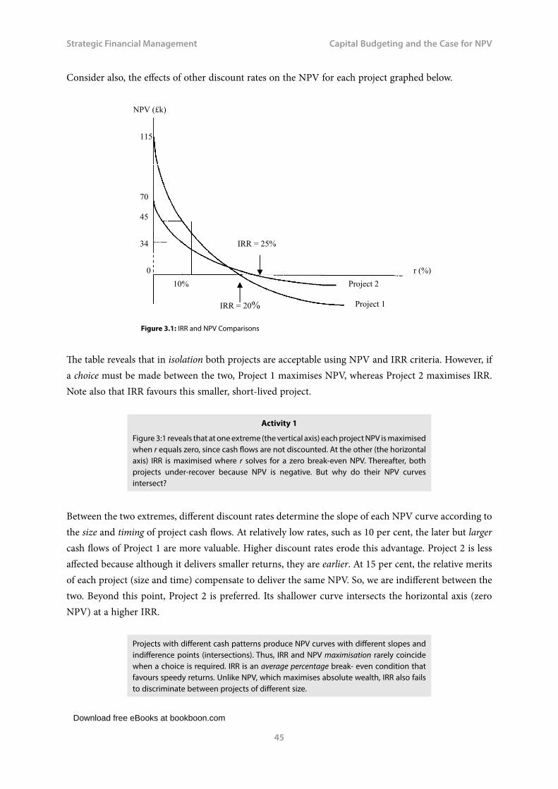
Consider also, the effects of other discount rates on the NPV for each project graphed below.
Figure 3.1: IRR and NPV Comparisons
The table reveals that in isolation both projects are acceptable using NPV and IRR criteria. However, if a choice must be made between the two, Project 1 maximises NPV, whereas Project 2 maximises IRR. Note also that IRR favours this smaller, short-lived project.
Activity 1
Figure 3:1 reveals that at one extreme (the vertical axis) each project NPV is maximised when r equals zero, since cash flows are not discounted. At the other (the horizontal axis) IRR is maximised where r solves for a zero break-even NPV. Thereafter, both projects under-recover because NPV is negative. But why do their NPV curves intersect?
Between the two extremes, different discount rates determine the slope of each NPV curve according to the size and timing of project cash flows. At relatively low rates, such as 10 per cent, the later but larger cash flows of Project 1 are more valuable. Higher discount rates erode this advantage. Project 2 is less affected because although it delivers smaller returns, they are earlier. At 15 per cent, the relative merits of each project (size and time) compensate to deliver the same NPV. So, we are indifferent between the two. Beyond this point, Project 2 is preferred. Its shallower curve intersects the horizontal axis (zero NPV) at a higher IRR.
Projects with different cash patterns produce NPV curves with different slopes and indifference points (intersections). Thus, IRR and NPV maximisation rarely coincide when a choice is required. IRR is an average percentage break- even condition that favours speedy returns. Unlike NPV, which maximises absolute wealth, IRR also fails to discriminate between projects of different size.

Download free eBooks at bookboon.com
Strategic Financial Management
46
Capital Budgeting and the Case for NPV
3.2 The Incremental IRR
Despite their apparent wealth maximisation defects, IRR project rankings that conflict with NPV can be brought into line by a supplementary IRR procedure whereby management:
Determine the incremental yield (IRR) from an incremental investment, which measures marginal profitability by subtracting one project’s cash inflows and outflows from those of another to create a sub-project (sometimes termed a ghost or shadow project).
To prove the point, let us incrementalise the data from Section 3.1.Two projects that not only differ with respect to their cash flow patterns (size and timing) but also their investment cost.
Project Year 0 Year 1 Year 2 Year 3 Year 4 Year 5 IRR(%) NPV (10%)
1 less 2 (35) (30) - 20 40 50 15% 11.1
You will recall that IRR maximisation favoured a higher percentage return on the smaller more liquid investment (Project1), whereas NPV maximisation focussed on higher money profits overall (Project 2). Now see how the incremental IRR (15%) on the incremental investment (Project 1 minus Project 2 = £35k) exceeds the discount rate (10%) so Project 1 is accepted. Moreover, this corresponds to Equation (1) on single project acceptance. The incremental NPV is positive (£11.1k) because its discount rate r < incremental IRR.
3.3 Capital Rationing, Project Divisibility and NPV
If finance is unconstrained, management should accept all projects with a positive NPV. But if capital is rationed and smaller projects with smaller NPVs can be replicated, or projects are divisible into fractional investments, we need to compare investments of different size by indexing their NPV per £1 invested using the following formula.
(3) NPVI = NPV / I0
The Profitability Index (NPVI)) then ranks projects, or proportions of them that maximise total NPV, relative to their cost, rather than their absolute surplus.

Download free eBooks at bookboon.com
Strategic Financial Management
47
Capital Budgeting and the Case for NPV
Activity 2
Using data from our previous Activity plotted in Figure 3.1, confirm the following (£k).
Project I0 NPV (10%) NPVI
1 (135) 45.4 0.336
2 (100) 34.3 0.343
Now assume the company has only £180,000 to invest. The projects are not mutually exclusive but they are infinitely divisible. Tabulate management’s optimum strategy.
The following table confirms that ranking projects by the NPV per £ method, rather than their individual NPV, maximises overall NPV and hence total corporate wealth.
Method Ranking Capital Cost NPV
NPV (£) 1 (135) 45.4
2 (45/100) (45) 15.4
Sub-optimal (180) 60.8
NPVI 2 (100) 34.3
1 (80/135) (80) 26.9
Optimal (180) 61.2
3.4 Relevant Cash Flows and Working Capital
So far, we have taken as given the cash flows that underpin DCF analyses. However, management need to determine those that are relevant to a project’s appraisal.
Relevant cash flows are based on the opportunity cost concept which defines the incremental net inflows if a project is accepted. The analysis incorporates outflows that are unavoidable, or inflows which are sacrificed elsewhere, if a project is accepted.
Thus, accounting concepts of historical cost and net book value (NBV) are irrelevant because they are sunk costs. Likewise, forecast income and expenses based on accrual accounting are irrelevant. Assets purchased five years ago for £10k with an NBV of £1k may be surplus to current requirements but with a market (opportunity) value of £9k and as a substitute for assets costing £12k they can reduce future project costs by £3k. Likewise, if the assets are used for this project, rather than another, then the project cash foregone must be included in the selected project’s opportunity flows if it is the next highest valued alternative (say £9.5k).
With regard to accounting income there is a timing issue; periodic turnover rarely corresponds to cash inflow because of credit sales. Expenses too, may be accrued or prepaid. There is also depreciation to consider.

Download free eBooks at bookboon.com
Click on the ad to read more
Strategic Financial Management
48
Capital Budgeting and the Case for NPV
Depreciation should always be added back to net accounting profits when they are used for project selection. It is a non-cash expense, not an incremental outflow; that part of earnings retained to recoup an investment’s cost (I0)) over its useful life. Since NPV analyses already subtract I0 from project cash flows (NPV = PV – I0) the use of profit after depreciation as a proxy for net cash inflow in project appraisal obviously double counts the investment’s cost.
Since our test for opportunity cost focuses upon differential costs, we must also incorporate adjustments for working capital investment designed to fuel projects when up and running.
Working capital is basically stock (inventory), debtors, plus cash, minus creditors. This net investment in current assets may differ for different project proposals, vary from year to year, or build up gradually Disinvestment may also occur beyond a project’s life, for example when debtors repay, creditors are satisfied and surplus inventory is sold on.
Working capital should be regarded as a cash outflow at the outset of a project’s life with adjustments in subsequent years for the net investment caused by project acceptance. At the end of a project’s life, the funds still tied up will be released for use elsewhere. Therefore, we show this amount as a cash inflow in the last year or whenever it is made available. The net effect of these working capital adjustments are to charge the project with the interest foregone (opportunity cost of capital) on the funds, which are invested throughout its entire life.
Som medarbetare i Riksbyggen vill vi att du ska känna att du är viktig och att du tydligt kan se hur du bidrar till att vi uppnår våra mål. Vi erbjuder dig stimulerande och utvecklande arbetsuppgifter i ett kreativt arbetsklimat. Inom Riksbyggen kan du som ekonom exempelvis arbeta som ControllerKundansvarig ekonomRedovisningsekonomByggekonomProjektekonomVill du utvecklas tillsammans med oss?Riksbyggen utvecklar, förvaltar och förbättrar rummen som du bor och arbetar i.
Hitta ditt jobb på
riksbyggen.se
Vi har koll påsiffrorna
Viktoria är ekonom på Riksbyggen

Download free eBooks at bookboon.com
Strategic Financial Management
49
Capital Budgeting and the Case for NPV
Activity 3
Never under estimate the role of working capital management in project appraisal. Select a random sample of published company accounts and you will observe that current assets represent more than 50 per cent of total capital investment for a significant number.
3.5 Capital Budgeting and Taxation
Another incremental cash flow, which we haven’t touched on, that may involve timing discrepancies affecting project selection and shareholder wealth, is corporate taxation.
We know that in the absence of tax, depreciation should be added back to accounting profits for DCF appraisal. It is a non-cash expense and not an incremental outflow. But if depreciation is a capital allowance that reduces taxable profits and because tax represents a cash outflow, we must include both in our calculation of net tax cash inflows.
Consider a project with an annual £100k cash return on a five year investment costing £300k with a 100 per cent straight-line capital allowance and a corporate tax rate of 25 per cent. We can compare the project’s annual post-tax profits with its true cash position as follows:
Annual Data(£k) Taxable Income Taxable Income (without any capital allowance)
Cashflow
Profit before depreciation 100 100 100
Capital allowance (20%) 60
Pre-tax profit 40 100
Corporation tax (25%) 10 25 (10)
Post-tax profit 30 75 90
If we do not deduct a capital allowance from the profit before depreciation (Column 2) the tax liability would be £25k (i.e. 25 per cent of £100k). And post-tax profit and net cash inflow would both equal £75k. However, with the capital allowance, an extra £15k cash flow is retained because the 25 per cent tax rate is applied to a profit figure of £40k adjusted for the annual capital allowance (£60k / 5). Consequently, the true annual cash flow is £90k.
Depreciation therefore acts as a tax shield if it is a capital allowance because it reduces a company’s net tax liability and increases its net cash inflow.

Download free eBooks at bookboon.com
Strategic Financial Management
50
Capital Budgeting and the Case for NPV
Of course, we have still not considered the timing discrepancy associated with deferred tax payments. These too, exert a positive bias on our DCF calculations. For example, assuming a twelve month delay, an accurate picture of the cash flow pattern for our five year project adjusted for relief, prior to any periodic net working capital adjustments, would be:
Cash Flows (£k) Year 0 Year 1 Year 2 Year 3 Year 4 Year 5 Year 6
Inflow - 100 100 100 100 100 -
Outflow (300) - (10) (10) (10) (10) (10)
Net Flow (300) 100 90 90 90 90 (10)
Once we incorporate working capital (if any) into the schedule, all that is required is to discount the net cash flows at the project’s opportunity cost of capital adjusted for inflation.
3.6 NPV and Purchasing Power Risk
If a firm seeks to maximise shareholder wealth and their consumption-investment preferences, its capital budgeting decisions must be inoculated from two types of purchasing power risk.
- Specific price rises that erode the real value of a project’s future net cash flows and diminish a firm’s operating capability and share value. Management must uplift current (real) cash flows by specific price adjustments if necessary, to produce a project’s forecast money flows.
- Inflation, that erodes consumption of goods and services generally, which must be reinstated by an upward revision of project discount rates if they ignore purchasing power losses. Nominal (real) interest rates that reflect zero inflation must be adjusted to money rates which reflect the expectations of investors who determine the market rate to compensate for this.
Irving Fisher (1930 op cit) defined the relationship between a market (money) interest rate (m) and a nominal (real) rate(r) given an annual compound inflation rate (i) as follows:
(4) (1 + m) = (1 + r) (1 + i)
So, that re-arranging terms:
(5) m = (1 +r)(1 + i) – 1 = the money rate,
(6) r = [(1 + m) / (1 + i)] – 1 = the real rate.
For example, if a project’s real (nominal) discount rate is 7.5 per cent and the annual rate of inflation is 7 per cent, the money (market) rate of interest used to discount a project’s money cash flows to determine a project’s NPV is given by Equation (5):

Download free eBooks at bookboon.com
Click on the ad to read more
Strategic Financial Management
51
Capital Budgeting and the Case for NPV
m = (1.075) (1.07) – 1 = 15%
Activity 4
Armed with this information, use Equation (6) to reverse the Fisher effect on the money rate (m = 15%) with an inflation rate (i= 7%) and prove that the real rate (r) equals 7.5 percent.
Review Activity
Your University intends to market a financial text priced at £60 over four years with the following demand pattern, forecast money flows and a 15 percent money cost of capital.
Year 1 Year 2 Year 3 Year 4Annual Demand 6,200 7,200 4,000 2,800
- Capital set-up investment of £100k with a residual value of £20k in year 4 - Variable production costs of £40 per text - Royalty costs of £20k in year one, £15k in year two and £10k in years three and four - Working capital investment of £80k recoverable in year 4 - Fixed cost recovery of £60,000 per annum that includes depreciation
Using NPV and NTV criteria, establish whether the University should proceed with the project.
Imagine yourself working with some of the sharpest and most creative brains in the transport and infrastructure industry, developing sustainable transport solutions that will change the future of society.
Imagine yourself working in a company that really believes that people are its driving force, fostering a culture of energy, passion and respect for the individual.
Imagine yourself working for the Volvo Group, a global leader in sustainable transport solutions with about 110,000 employees, production in 18 countries and sales in about 190 countries. A place where your voice is heard and your ideas matter.
Together we move the world.
www.volvogroup.com/career
SHAPINGANOTHER FUTURE

Download free eBooks at bookboon.com
Strategic Financial Management
52
Capital Budgeting and the Case for NPV
First, the data needs to be reformulated in terms of relevant cash flows.
- Depreciation must be removed from fixed costs because it is not a cash flow. - Fixed costs should only be included if relevant i.e. incurred only if the project is undertaken. - Residual asset values including working capital are always relevant because they defray the
final project cost through their future opportunity value to the company, or sale on the market.
- Because universities (at least in the UK) are charities that do not pay tax, we can ignore it.
Second, let us assume fixed cost relevancy (the worst case scenario) whereby:
Fixed costs minus depreciation = £60k – £20k = £40k per annum
[Annual depreciation = capital cost less residual value / project life = £100k–£20k / 4 = £20k]
Finally, we can tabulate the data to calculate NPV and NTV.
The table overleaf reveals the project is profitable, even if burdened with fixed costs. The NTV confirms an NPV surplus in terms of economic value added four years from now. Obviously, if fixed costs are genuinely “fixed” (incurred irrespective of project acceptance) they should be ignored. And in this case the NPV and NTV would be higher still (£137.57k and £240.6k respectively).
Perhaps you can confirm this?

Download free eBooks at bookboon.com
Strategic Financial Management
53
Capital Budgeting and the Case for NPV
Relevant Money Cash Flows (£k)
Year 0 1 2 3 4 Points to note
Capital Cost (100) 20 (residual value)
Contribution - 124 144 80 56 (sales less variable costs)
Fixed Costs - (40) (40) (40) (40) (less depreciation)
Royalties - (20) (15) (10) (10) (given)
Working Capital (80) 80 ((residual value)
Net Inflow (180) 64 89 30 106
DCF Factors 1.0 0.870 0.756 0.658 0.572 [(1 / (1+0.15)t]
Net DCF (180) 55.68 67.28 19.74 60.63
NPV and NTV 23.33 40.80 [NTV=NPV (1+r)n]
3.7 Summary and Conclusions
Unless management is confronted by a single project with one initial outflow followed by subsequent net inflows, the IRR may produce sub-optimal investment decisions, whereas the NPV maximisation of all a firm’s projects, which discounts relevant incremental money cash flows at the money (market) rate of interest, should maximise wealth. Differences arise because the latter is a measure of absolute wealth, whilst the former is a relative measure. The validity of the two models also hinges upon their respective assumptions concerning borrowing and reinvestment rates. NPV calculations use the opportunity cost of capital, whilst IRR assumes that capital cost and re-investment rates equal a project’s IRR, usually without any economic foundation whatsoever.
Of course, we must remember that even if NPV incorporates relevant cash flows, taxation and price changes it is still only a model that simplifies a complex world of risk and uncertainty. So, how do management deal with these phenomena to maximise shareholder wealth?

Download free eBooks at bookboon.com
Click on the ad to read more
Strategic Financial Management
54
The Treatment of Uncertainty
4 The Treatment of UncertaintyIntroduction
So far, our capital budgeting analyses have assumed complete certainty, whereby relevant money cash flows and money discount rates can be specified in advance. But what if a plurality of future cash flows and discount rates are possible? How do management select investments that maximises shareholder wealth in this real world of risk and uncertainty?
Let us begin with a conceptual clarification and a few definitions.
Risk and uncertainty both refer to situations with more than one outcome. However, risk defines future events that can be objectively specified in advance based on prior knowledge; an obvious example being the throw of a dice. Uncertainty, which characterises most business decisions, relates to events whose probabilities cannot be predicted with accuracy.
What management require, therefore, are quantitative techniques that transform uncertainty to quasi-risk, which assumes a range of possible outcomes and assigns subjective probabilities to the likelihood of each occurring.
Var med och utveckla Stockholm!
Vår vackra huvudstad växer som aldrig förr och stockholmare i alla åldrar behöver allt från en fungerande infrastruktur till renhållning, förskolor och äldreomsorg. Verksamheten finns överallt i staden och måste fungera dygnet runt, varje dag. Nu behöver vi dig som vill vara med och skapa ett Stockholm i världsklass!
Läs mer på stockholm.se/jobb

Download free eBooks at bookboon.com
Strategic Financial Management
55
The Treatment of Uncertainty
We should also note that a project’s overall uncertainty or total risk embraces:
- Business risk that relates to the variability of future cash flows arising from an investment’s fundamental characteristics, as well as changing economic conditions.
- Financial risk associated with a project’s funding and how the earnings distributed to investors determine the company’s cost of capital (discount rate).
Since the former determines the latter (without profits how can you reward investors?) financial risk need not concern us yet. Cost of capital is also better left until we deal with security pricing in Part Three. So, first let us focus on the treatment of business risk,
4.1 Dysfunctional Risk Methodologies
The following risk techniques are popular with management. But unfortunately they fail to maximise shareholder wealth.
- Modifications to the cut-off rate for investment that adds a risk premium the discount rate. - Point estimates such as best, worst or most likely net cash inflow; Minimax, which focuses
upon the best outcome under the most adverse conditions; Laplace criteria, which select the most favourable simple average of a three point estimate; Probability estimation which applies probabilities to three point forecasts to produce the best weighted average (subject to the proviso that the sum of the probabilities equals one).
Suffice it to say that if the cut-off (discount) rate is based on a market rate, it already factors in business risk. So, adding a premium duplicates uncertainty. Turning to the variability of cash flows point estimations and their derivatives may also be counterproductive. The worst scenario may be improbable, but if it materialises then it may be catastrophic for the firm.
4.2 Decision Trees, Sensitivity and Computers
Look at any financial text and you will also find decision trees, sensitivity analyses and computer simulation techniques. However, these do not quantify risk. Rather they manipulate risk-adjusted data to assess their effect on an investment’s viability.
Decision trees provide a mind map of uncertain project cash flows branch out from an investment (hence its name) and may proliferate beyond a three-point analysis. Conditional probabilities are attached to a sequence of likely future events. The branches of the trunk arise from previous managerial decisions (control factors) and chance (uncontrollable factors).

Download free eBooks at bookboon.com
Strategic Financial Management
56
The Treatment of Uncertainty
Sensitivity analysis deconstructs cash data that comprise an initial NPV computation into estimates of its component parts. Each variable is then analysed sequentially, using partial equilibrium analysis. By holding all other variables constant and gauging the impact on the appropriate investment criteria of percentage changes to the variable under observation, its critical value is established.
Computer simulation can be used in conjunction with decision trees, sensitivity analysis, or any technique, to calculate quickly innumerable permutations of probabilistic cash flows.
As tools, however, decision trees, sensitivity analyses and computer simulation are only as sound as the data upon which they are based. So, let us move beyond three point estimation.
4.3 Mean-Variance Methodology
Forecast data that extends beyond point estimations to multi-valued outcomes may be converted to quasi-risk using the more sophisticated technique of mean-variance analysis. Based on classical probability theory, management assume cash flows are random variables, which conform to a normal distribution with a symmetrical bell-shaped curve as follows:
Figure 4.1: The Symmetrical Normal Distribution, Area under the Curve and Confidence Limits
The mean is derived by first multiplying a spectrum of annual cash flows Ci by respective probabilities Pi (subject to the proviso that ∑Pi =1.0). Then the products Ci Pi for any number of cash flows (n) are summated to derive an expected monetary value (EMV) at time period t:

Download free eBooks at bookboon.com
Click on the ad to read more
Strategic Financial Management
57
The Treatment of Uncertainty
Next, the annual EMV series is discounted over the appropriate periods at a risk-free rate (avoiding double-counting) to determine its expected PV, (EPV). From this we subtract the investment cost, Io, to obtain a project’s expected NPV, (ENPV) in the usual manner:
Obviously, EMV time-series and ENPV analyses improve upon point estimates. But project selection using ENPV maximisation alone cannot minimise risk because it doesn’t calibrate the degree to which cash flows vary around their mean (business risk) or managerial reaction to this variability. To resolve the dilemma, the standard deviation is used to measure the average dispersion of cash flows from their EMV. Management then compare the standard deviation with the expected return to assess a project’s risk-return profile; the interpretation being that for a given return, the lower the standard deviation the lower the risk and vice versa.
The financial industry needs a strong software platformThat’s why we need you
Meet Lars and other employees at simcorp.com/meetouremployees
Mitigate risk Reduce cost Enable growthsimcorp.com
Working at SimCorp means making a difference. At SimCorp, you help create the tools
that shape the global financial industry of tomorrow. SimCorp provides integrated
software solutions that can turn investment management companies into winners.
With SimCorp, you make the most of your ambitions, realising your full potential in
a challenging, empowering and stimulating work environment.
Are you among the best qualified in finance, economics, computer science or mathematics?
Find your next challenge at www.simcorp.com/careers
“When I joined SimCorp, I was very impressed with the introduc-tion programme offered to me.”

Download free eBooks at bookboon.com
Strategic Financial Management
58
The Treatment of Uncertainty
Assuming statistically normal returns, the standard deviation is determined as follows:
- Calculate the mean of the distribution (EMV) by multiplying each variable’s value by its probability of occurrence and adding the products.
- Subtract the EMV from each possible value and square the result. - Multiply each squared deviation around the mean by its probability to determine
certainty equivalents and add them together. This sum is the variance. - Calculate the square root of the variance. This is the standard deviation
In most texts the standard deviation (SD) is denoted by the Greek letter s or the term ÖVAR and the variance by s2 and VAR respectively. Using these conventions we can express the risk characteristics of a cash flow distribution algebraically given:
The project variance equals the weighted average of the sum of the squared deviations of each observable cash flow (Ci) from its mean cash flow (EMV) where each weight is represented by the cash flow’s probability of occurrence (Pi). Because normal distributions are symmetrical (Figure 4.1) we square the deviations, otherwise their summation would be self-cancelling with a mean deviation of zero. However, squaring also introduces a scale change to the variables in relation to the EMV. This is remedied by calculating the square root of the variance to produce the standard deviation, which is a measure of dispersion expressed in identical units to the mean of the distribution (£say).
4.4 Mean-Variance Analyses
To understand the role of mean-variance calculations in capital budgeting, consider the following calculations of EMV, s2 and s for a project’s possible contribution per unit.

Download free eBooks at bookboon.com
Strategic Financial Management
59
The Treatment of Uncertainty
Ci Pi CiPi (C i – EMV)2 Pi (Ci – EMV)2 Pi
£ £
8 0.1 0.80 3.61 0.1 0.361
7 0.2 1.40 0.81 0.2 0.162
6 0.4 2.40 0.01 0.4 0.004
5 0.3 1.50 1.21 0.3 0.363
(1.0)
Expected Monetary Value (EMV) £6.10 Variance (VAR = s2) = 0.890
S.D. (ÖVAR = s) = £0.943
The first point to note is that best, worst and most likely states of the world all differ from the EMV of the cash flow distribution. Second, the most optimistic outcome is least likely to occur (£8 with a probability of 0.1).There is also a 70 percent chance of cash flows falling short of their EMV. So, what does the standard deviation of £0.943 tell us?
Refer back to Figure 4.1 which sketched the area under the standard normal curve and the probability that a variable’s value lies within a number of standard deviations away from the mean. Because these probabilities are the same for any normal distribution they have long been quantified in tables based on the z statistic, which standardises any variable’s actual deviation from the mean by reference to the standard deviation. For a particular cash flow (Ci) drawn from a distribution with known mean and variance:
(5) z = Ci – EMV / s (Ci)
We then consult the table to establish the area under the normal curve between the right or left of z (plus or minus) to estimate the probability that the expected cash flow will be a given number of standard deviations away from the mean. Since a normal distribution is symmetrical, the probability of a variable deviating above and below the mean is given by 2z.
Activity 1
Seek out a z table, and with the previous sample data (EMV of £6.10 and s of £0.943) let us establish the probability of project contributions ranging from £6.50 to £5.50.
To determine the probability of contributions deviating above or below the mean as specified, we must first calculate the following z statistics using Equation (5).
£6.10 is (6.10 – 6.10) / 0.943 = zero s from the mean (obviously)
£6.50 is (6.50 – 6.10) / 0.943 = +0.42 s from the mean
£5.50 is (5.50 – 6.10 / 0.943 = -0.64 s from the mean

Download free eBooks at bookboon.com
Strategic Financial Management
60
The Treatment of Uncertainty
Next we consult the table for the area under the standard normal curve where z equals zero, 0.42 and 0.64 (i.e. 0.5000, 0.3372 and 0.2611).The mean-z areas are 0.1628 and 0.2389 respectively (i.e. 0.5000–0.3372 and 0.5000–0.2611). Thus, the total area under the curve, between +0.42 and -0.64, equals 0.4017 (i.e. 0.1628+0.2389). So, there is a roughly a 40 percent probability of the contribution ranging from £6.50 to £5.50.
Activity 2
Over many years, surveys reveal that probability analysis has gained ground (see Arnold and Hatzopoulus, 2000) one reason is that the risk-return profile for any normal distribution conveniently conforms to predetermined confidence limits.
Referring to Figure 4.1 and your z table, confirm that the percentage probability of any cash flow lying one, two, or three standard deviations above or below the EMV is given by the following confidence limits:
2 x 0.3413 for - s to +s = 68.26%
2 x 0.4772 for -2s to +2s = 95.44%
2 x 0.4987 for -3s to +3s = 99.74%
Applied to our previous Activity, now confirm there is a 99.74 percent probability that the distribution with an EMV of £6.10 and a standard deviation of £0.943 will have a contribution within the following range:
EMV ± 3s = £6.10 + [3 (£0.943)] to £6.10 – [3 (£0.943] = £8.93 to £3.27
4.5 The Mean-Variance Paradox
Returning to the normative objective of financial management, if capital is rationed or investments are mutually exclusive and choices must be made, project selection using either the highest expected return or the lowest standard deviation does not necessarily maximise wealth or minimise risk. Consider the risk-return profiles of two projects (A and B):
ENPVA = £50k and sNPVA = £30k ENPVB = £200k and sNPVB = £90k
ENPV selects B but sNPV selects A. But which maximises wealth and which is less risky?
To resolve the paradox, what we need is a relative rather than absolute statistical measure of project variability around its mean value that builds on confidence limits. One lifeline is the coefficient of variation:
(6) Coeff. V = sNPV / ENPV
This is interpreted as the smaller the coefficient, the lower the risk. Applied to the data:
Coeff VA = 30/50 = £0.60 > Coeff VB = 90/200 = £0.45

Download free eBooks at bookboon.com
Click on the ad to read more
Strategic Financial Management
61
The Treatment of Uncertainty
Thus, Project A seems more risky than Project B because it involves £0.60 of risk ((s NPV) for every £1.00 of ENPV, rather than £0.45 (s NPV) for every £1.00 of ENPV.
The coefficient of variation is important because it tries to encapsulate the fundamental, twin objectives of corporate wealth maximisation, which we can summarise as follows:
WEALTH MAXIMISATION: MAX: ENPV and MIN: NPV
MAX: ENPV, given NPV (i.e. maximise the ENPV for a given degree of variability)
MIN: NPV, given ENPV(i.e. minimise the variability of returns for a given ENPV).
Unfortunately, the coefficient of variation is not a selection criterion because it ignores investment size, thereby assuming that managerial risk attitudes are constant, even though intuitively we know that rational investors become more risk averse as their stake increases. Add zeros to the previous project data and note that the coefficients remain the same.
To remove this anomaly, management must predetermine a desired minimum ENPV for any investment (Io) expressed as a profitability index to satisfy all their corporate investors.

Download free eBooks at bookboon.com
Strategic Financial Management
62
The Treatment of Uncertainty
Then comparison must be made to expected indices for proposed investments, incorporating confidence limits based upon an appropriate number of standard deviations. These define subjective managerial risk attitudes. So, the objective function for project selection becomes:
(7) MAX: (ENPV – nsNPV) / I0 ≥ MIN: NPV / I0
Activity 3
Assume management require a benchmark [MIN:NPV / I0] = £0.15 to satisfy stakeholders. Use the previous data to derive the left-hand side of Equation (7) three standard deviations from the mean for each project (A and B) that cost £100k and £120k, respectively.
Which project, if either, is acceptable?
Recall that Project B was preferable using the coefficient of variation. Note now, however, that if management require almost complete certainty (99.74%) neither project is acceptable using the expected profitability index, although Project A minimises losses.
Project £(ENPV – 3sNPV) / I0≥ MIN: £NPV / I0 Decision
A 50–90/100 = (0.40) > 0.15 Reject
B 200–70/120= (0.58) > 0.15 Reject
4.5 Certainty Equivalence and Investor Utility
The ultimate test of mean-variance analysis depends upon investor risk attitudes. In our previous example, risk aversion signals rejection. Yet risk-seekers (speculators) might actually accept Project B because investing £120k rather than £100k might yield £470k as opposed to £140k three standard deviations above the mean, whilst the equivalent downside loss is only £70k compared with £50k. So, how do we circumvent this risk-return paradox?
One solution is to dispense with the standard deviation altogether and calibrate an individual’s subjective attitude towards risk expressed in terms of units of utility, rather than monetary gains and losses, associated with investments. Given this utility function, we then calculate the certain cash equivalent of the distribution of uncertain cash flows discounted at the risk-free rate for any project and assess its viability for the investor using wealth maximisation criteria.
Consider the data set overleaf that signals a project acceptance using Equation 2 as follows:ENPV = S EPV-I0 = £67.5k – £50k = £17.5k

Download free eBooks at bookboon.com
Strategic Financial Management
63
The Treatment of Uncertainty
Now look at the utility data, which rejects the project. To understand why, assume you ask the investor to enter a game with a 50/50 chance of receiving nothing or £100k to which we attach arbitrary utility values of zero and one respectively. Next you ask what the game is worth. The investor’s response is £40k. This represents their indifference between certain cash and the game. Thus, three points on the individual’s utility curve associated with certain cash equivalents can be obtained (shown in bold) based on the following equation of indifference:
(8) Certain Utility = Probabilistic Utility + Probabilistic Utility U (£40,000) = [0.5 U (£0) = 0.5(0)] + [0.5 U (£100,000) = 0.5 (1.0)] = 0.5
If the game’s entry price was £50k he would walk away. However, other scale points, such as £50k (with a value of 0.65 say) can be established by gaming cash amounts for known utilities. If the procedure is repeated exhaustively, the investor’s utility function consistent with his risk attitude will emerge, like the profile plotted in Figure 4.2 overleaf.
The curve’s geometry (if not its specific values) applies to any rational investor. Except for small gambles relative to current wealth, it reveals risk aversion, denoted by the convex shape of the function (looking from above). Near the origin, the concave sector denotes risk preference. Note that the utility of one for £100k is only twice that of 0.5 for £40k (which we originally calculated) but more than half the utility of £200k, as risk aversion sets in.
Returning to our example, the application of Equation (8) using the investor’s utility curve reveals that despite a positive ENPV the project should be rejected. The utility of its cost exceeds the cash equivalent of the expected utility of the discounted cash flow distribution.
U (£50,000) = 0.65 > S{0.167+0.300+0.260+(0.075)+(0.152)} = 0.5 = U (£40,000)
Review Activity
Summarise the problems that confront practising financial managers who use certainty cash equivalents, rather than mean-variance as a basis for investment appraisal.
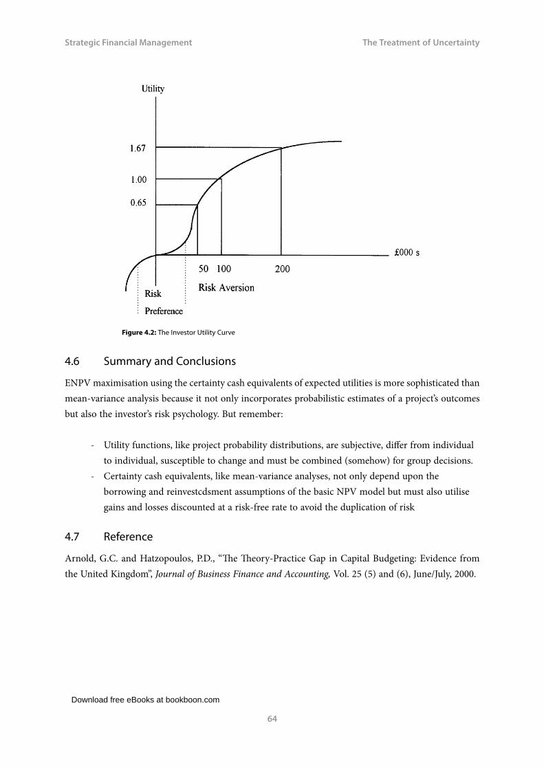
Download free eBooks at bookboon.com
Strategic Financial Management
64
The Treatment of Uncertainty
Figure 4.2: The Investor Utility Curve
4.6 Summary and Conclusions
ENPV maximisation using the certainty cash equivalents of expected utilities is more sophisticated than mean-variance analysis because it not only incorporates probabilistic estimates of a project’s outcomes but also the investor’s risk psychology. But remember:
- Utility functions, like project probability distributions, are subjective, differ from individual to individual, susceptible to change and must be combined (somehow) for group decisions.
- Certainty cash equivalents, like mean-variance analyses, not only depend upon the borrowing and reinvestcdsment assumptions of the basic NPV model but must also utilise gains and losses discounted at a risk-free rate to avoid the duplication of risk
4.7 Reference
Arnold, G.C. and Hatzopoulos, P.D., “The Theory-Practice Gap in Capital Budgeting: Evidence from the United Kingdom”, Journal of Business Finance and Accounting, Vol. 25 (5) and (6), June/July, 2000.

Download free eBooks at bookboon.com
Click on the ad to read more
Strategic Financial Management
66
Equity Valuation and the Cost of Capital
5 Equity Valuation and the Cost of Capital
Introduction
Part Two provided a detailed explanation of the investment decision with only oblique reference to the finance decision, which determines a company’s cost of capital (discount rate) designed to maximise shareholder wealth. But if wealth is to be maximised, management must determine what return their shareholders require from an investment and then only accept projects that have a positive NPV when discounted at that rate.
There is also the question as to what cut-off rate should apply to investment proposals if corporate finance were obtained from a variety of sources, other than ordinary shares? Each stakeholder requires a rate of return that may differ from the equity market and may be unique. In this newly leveraged situation, the company’s overall cost of capital (rather than its cost of equity) measured by its weighted, average cost of capital (WACC) would seem to be the appropriate investment acceptance criterion.
Designed for high-achieving graduates across all disciplines, London Business School’s Masters in Management provides specific and tangible foundations for a successful career in business.
This 12-month, full-time programme is a business qualification with impact. In 2010, our MiM employment rate was 95% within 3 months of graduation*; the majority of graduates choosing to work in consulting or financial services.
As well as a renowned qualification from a world-class business school, you also gain access to the School’s network of more than 34,000 global alumni – a community that offers support and opportunities throughout your career.
For more information visit www.london.edu/mm, email [email protected] or give us a call on +44 (0)20 7000 7573.
Masters in Management
The next step for top-performing graduates
* Figures taken from London Business School’s Masters in Management 2010 employment report

Download free eBooks at bookboon.com
Strategic Financial Management
67
Equity Valuation and the Cost of Capital
Given the normative assumption of financial management, the purpose of Part Three is straightforward. How does a firm maximise corporate wealth by securing funds at minimum cost that not only provides shareholders with their desired rate of return, once investment takes place, but also satisfies the expectations of all capital providers?
To set the scene, Chapter Five provides an explanation of the most significant explicit, opportunity cost of external funding available to management. The cost of ordinary shares measured by their rate of return, often termed the equity capitalisation rate or yield.
5.1 The Capitalisation Concept
In Chapter Two we defined an investment’s present value (PV) as its relevant periodic cash flows (Ct) discounted at a constant cost of capital (r) over time (n). Expressed algebraically:
The equation has a convenient property. If the investment’s annual cash receipts are also constant and tend to infinity, (Ct = C1 = C2 = C3 = C∞) their PV simplifies to the formula for the capitalisation of a constant perpetual annuity:
The term r is called the capitalisation rate because the transformation of a cash flow series to value (i.e. capital) is termed “capitalisation”. With data on PV∞ and r, or PV∞ and Ct, we can also determine values for Ct or r respectively. Rearranging Equation (2) with one unknown:
(3) Ct = PV∞ . r
(4) r = PV∞ / Ct
These PV equations are vital to your understanding of various share valuation models, which define the possible cost of equity as a managerial cut-off rate for investment. So, let us define the models beginning with dividend valuation.

Download free eBooks at bookboon.com
Strategic Financial Management
68
Equity Valuation and the Cost of Capital
5.2 Single-Period Dividend Valuation
Assume you hold a share for one year, at the end of which a dividend is paid. You then sell the share ex-div, which means the new investor does not receive the dividend (you do) as opposed to cum-div, where the dividend is incorporated into price. Your current ex-div price, (P0) is defined by the expected year-end dividend (D1) plus the expected year-end share price (P1) discounted at the appropriate rate of return for shares in that risk class, the cost of equity (Ke). Thus, we have the single-period dividend valuation model:
(5) P0 = (D1 + P1) / 1 + Ke = [(D1 / 1 + Ke) + (P1 / 1 + Ke)]
Sequentially, if the new investor holds the share for a further year, then their ex-div price on acquisition (i.e. dated when you sold it) is also given by the single- period model.
(6) P1 = [(D2 / 1 + Ke) + (P2 / 1 + Ke)]
Note however that if you held the share for two years, its current ex-div price would be the discounted sum of two dividends and the ex-div price at the end of year two, as follows:
(7) P0 = [(D1 / 1 + Ke) + (D2 / 1 + Ke)2 + (P2 / 1 + Ke)
2]
5.3 Finite Dividend Valuation
Assuming the cost of equity Ke is constant; the current ex-div price of a share held for any finite number of years (n) and then sold equals:
(8) P0 = [(D1 / 1 + Ke) + (D2 / 1 + Ke)2 + … + (Dn / 1 + Ke)
n] + (Pn / 1 + Ke)n
Rewritten, this defines the finite-period, dividend valuation model:
where Pn equals the ex-div value at time period n, determined by the discounted sum of subsequent dividends.
(10) Pn = [{Dn+1/(1+Ke)n+1} + {Dn+2 /(1+Ke)
n+2} + …]

Download free eBooks at bookboon.com
Click on the ad to read more
Strategic Financial Management
69
Equity Valuation and the Cost of Capital
Activity 1
A potential shareholder anticipates a dividend per share of 10 pence and 11 pence in years one and two respectively, whereupon the shares are expected to be sold ex div for £3.00 each. If the equity capitalisation rate is 20 percent per annum, confirm that the maximum current ex-div price at which the shares should be purchased is £2.24.
5.4 General Dividend Valuation
If distributions tend to infinity, then by definition the final term of Equation (9) disappears altogether because the share is never sold. This is the general dividend valuation model:
5.5 Constant Dividend Valuation
Finally, if we assume that dividends are constant in perpetuity (Dt = D1 = D2 = D3 …= D∞) and Ke is constant then the general model simplifies to the constant dividend valuation model.
(12) P0 = D1 / Ke
Masterstudienplätze in Holland Man and Health• Biomedical Sciences• Cognitive Neuroscience• Medical Biology• Molecular Life Sciences• Molecular Mechanisms of Disease
www.internationalmasters.eu/bb
Nature and Science• Information science• Biology• Chemistry• Computing Science• Environmental Sciences• Mathematics• Natural Science• Physics and Astronomy

Download free eBooks at bookboon.com
Strategic Financial Management
70
Equity Valuation and the Cost of Capital
5.6 The Dividend Yield and Corporate Cost of Equity
We stated earlier that an appreciation of equity valuation models is a pre-requisite for understanding why shareholder returns provide the management of an all-equity firm with its cut-off rate for investment. To prove the point, let us rearrange the terms of Equation (12).
(13) Ke = D1 / P0
We have now defined the dividend yield published daily by the financial press throughout the world from stock exchange listings. Whilst the yield is based on an abstract constant dividend model, its use by investors as a corporate performance indicator is rational.
In an uncertain world where future dividend or price movements are unknown, it is reasonable to assume that without information to the contrary, future returns should at least equal today’s ratio of a company’s latest dividend to current share price. As a percentage, this dividend yield also enables investors to compare a company’s performance over time, with its competitors, or the market, to establish whether its shares are over or under valued.
A “golden” investment rule is the higher the risk, the higher the return and lower the price. For example, a firm declares a 20 pence dividend on shares currently trading at £2.00. The yield is 10 per cent. But shareholders interpret the dividend as “bad” news and after panic selling, price falls to £1.00. So, the yield doubles, not because of improved performance but increased risk. Investors are now paying less for the same dividend.
Management ignore dividend yields at their peril
Because dissatisfied shareholders can always seek investment opportunities elsewhere, the percentage dividend for every £100 they invest in a company should represent a managerial benchmark for accepting new projects of equivalent risk. The yield also represents a minimum project return if management retain profits for reinvestment, rather than pay a dividend. Recalling Fisher’s Separation Theorem and Agency Theory, firms that cannot maintain yields should distribute profits for shareholders to reinvest on the capital market. To summarise:
The current dividend yield is an opportunity cost of capital which equals the minimum cut-off (discount) rate for new investment in an all-equity firm.

Download free eBooks at bookboon.com
Strategic Financial Management
71
Equity Valuation and the Cost of Capital
5.7 Dividend Growth and the Cost of Equity
For a company, the shareholder concept of maintainable yield based on the constant dividend model provides a convenient discount rate. Unfortunately, it is too simplistic. Assuming D1 = D2 = D3 and so on, implies either a 100 percent dividend pay-out ratio or zero-growth, both of which are rarely observed in the real world. Most firms retain a proportion of earnings for profitable reinvestment to enhance shareholder wealth through dividend growth and capital gains. So, how does this affect the yield as a cut-off rate for investment?
Beginning with a valuation model let us assume that through retention financed investment dividends now grow at a constant annual compound rate (g) in perpetuity. Leaving aside the detailed mathematics (that you can download elsewhere) M.J. Gordon (1958) proved that the current ex-div price becomes:
(14) P0 = D1 / Ke -g (subject to the non-negativity constraint that Ke >g)
The Gordon constant growth dividend model defines the current ex-div share price by capitalising next year’s dividend at the amount by which the desired equity return exceeds the constant rate of growth in dividend.
For example, if we assume that the next dividend per share is 20 pence, the shareholders’ rate of return is 10 percent per annum and the annual growth rate is five percent
P0 = D1 / Ke -g = £0.20 / (0.10 – 0.05) = £4.00
Activity 2
Take growth out of the previous equation or use Equation (12) for the constant dividend model to confirm that P0 is only £2.00. What does this reveal?
The two equations illustrate an important consideration for rational investors when buying shares, namely how growth potential can uplift equity value.
Rearrange the terms of Equation (14) and we can also isolate the impact of constant growth on the shareholders overall return.
(15) Ke = (D1 / P0) + g
So now, the cost of equity as a managerial discount rate equals a dividend expectation divided by current share price, plus a premium for growth. Using our previous example:
Ke = (£0.20 /£4.00) + 0.05 = 5% + 5% = 10%

Download free eBooks at bookboon.com
Click on the ad to read more
Strategic Financial Management
72
Equity Valuation and the Cost of Capital
5.8 Capital Growth and the Cost of Equity
Because dividend growth increases price, we can reformulate Equations (14) and (15) by
focussing on the capital gain impact on equity value and the corporate cut-off rate rate.
If share price grows at a constant annual rate G = (P1 – P0) / P0 then next year’s price:
(16) P1 = P0 (1 + G)
From Equation (14) we also know that the current price based on dividend growth (g):
(14) P0 = D1 / Ke -g
So, logically share price one year from now must equal:
(17) P1 = D2 / Ke -g = D1 (1+g) / Ke -g

Download free eBooks at bookboon.com
Strategic Financial Management
73
Equity Valuation and the Cost of Capital
Because the same share cannot sell at different prices, it follows from Equation (16) that the dividend growth rate (g) must equal (G) the annual growth in share price (capital gain). Equations (16) and (17) can therefore be redefined as follows:
(18) P1 = P0 (1+g)
A comparison of Equations (16) and (18) reveals that if share price grows at a rate G, this must equal g, the annual growth in dividends. If we substitute G for g into Equation (14), this produces a dividend-capital gain model equivalent to the Gordon growth model.
(19) P0 = D1 / Ke -G
The current ex div share price is determined by capitalising next year’s dividend at the amount by which the desired rate of return on equity exceeds the percentage capital gain.
Activity 3
If a company’s forecast dividend is 20 pence per share, price is expected to grow at five percent per annum, and the equity capitalisation rate is 10 per cent:
P0 = D1 / Ke -G = £0.20 / (0.10 – 0.05) = £4.00
Use the Gordon growth model to confirm that the current ex-div price still equals £4.00
Turning now to an equity capitalisation rate, which incorporates capital gains as a managerial investment criterion, we can substitute G for g into Equation (14) and rearrange terms so that:
(20) Ke = (D1 / P0) + G [from P0 = D1 / Ke -g and Ke = (D1 / P0) + g ]
This equation states that the total cost of equity comprises a dividend yield one year hence (D1/P0), plus a capital gain yield [G = (P1 – P0) / P0] equivalent to the growth in dividends (g).
Activity 4
If a company currently trading at £4.00 per share with a forecast 20 pence dividend is expected to grow at five percent per annum, confirm that the equity capitalisation rate is 10 per cent using the appropriate dividend and capital gain models.
5.9 Growth Estimates and the Cut-Off Rate
So far so good, but if management wish to finance future projects by retaining profits in their quest for shareholder wealth, how do they calculate the growth rate?

Download free eBooks at bookboon.com
Strategic Financial Management
74
Equity Valuation and the Cost of Capital
Obviously, dividend and capital gains are rarely constant, which gives rise to complex valuation models that are beyond the scope of this text. But even if they are uniform, management still need annual growth estimators. Since the future is so uncertain, a simple solution favoured by management is to assume that the past and future are interdependent. Without information to the contrary, Gordon (op cit) believed that a company’s anticipated growth should be determined from its financial history. Consider the following data:
Year Dividend per Share (pence)
2005 20
2006 22
2007 24.2
2008 26.62
2009 29.28
Using the formula (Dt-Dt-1)/Dt-1 we can determine annual dividend growth rates
Year Annual Growth Rate
2005–6 (22/20) -1 = 0.1
2006–7 (24.2/22) -1 = 0.1
2007–8 (26.62/24.2) -1 = 0.1
2008–9Total
(29.28/26.62)-1 = 0.1 0.4
The average periodic growth rate, as an estimator of g, is therefore given by:
g = 0.4 / 4 = 10%
Alternatively, we can calculate dividend growth by solving for g in the following equation and rearranging terms.
20 pence (1+g)4 = 29.28 pence.
:(1 + g) = 4√ (29.28/20.00)
g = 1.10 – 1.00 = 0.10 = 10%

Download free eBooks at bookboon.com
Click on the ad to read more
Strategic Financial Management
75
Equity Valuation and the Cost of Capital
Activity 5
Using the previous data and the appropriate equations, confirm that the forecast dividend for 2010 should be 32.21 pence. If shares are currently priced at £2.68 and dividends are expected to grow at ten percent per annum beyond 2010, confirm that the equity capitalisation rate (managerial cut-off rate for new investment) is 22 per cent.
5.10 Earnings Valuation and the Cut-Off Rate
Whether or not growth is incorporated into the model, there is still no consensus as to whether dividends alone determine a share’s value and hence the firm’s cut-off rate for investment.
As long ago as 1961, the Nobel economic prize winners, Franco Modigliani and Merton Miller (MM) argued that given the problems of estimating retention-financed dividend growth, why not assume that dividends and retentions are perfect economic substitutes? Because if so; a company’s share price and capitalisation rate can be determined by its overall earnings, rather than dividend policy. Since the future is uncertain, they also recommended a one period model.
According to MM, the current ex div share price (P0) equals the anticipated earnings per share (E1) plus the ex div price (P1) at the end of the year, discounted at the shareholders’ rate of return (Ke).Algebraically, their single-period earnings model is:
(21) P0 = (E1 + P1) / 1 + Ke = [(E1 / 1 + Ke) + (P1 / 1 + Ke)]
at
Ready to use youR talent?Future FiFteen graduate programme
Arla is welcoming talented, ambitious and global-minded graduates to join our unique graduate programme and pursue an international career.
PeRsonal develoPment thRough challenging woRkThe programme consists of three rotations, each lasting eight months. When changing rotation, you will enter a new position and become responsible for a project or a range of tasks that are critical to the business or have direct impact on our daily operations. At least one of the rotations will take place at a location outside your home country.
We will challenge you to work both independently and in teams, to face complex business scenarios and to keep focus in an ever-changing environment. When you have successfully completed your programme, you have the capability, both personally and professionally, to take on significant responsibility within our organisation.
To become a Future Fifteen you need to be a recent graduate with a university degree.
aRe you a FutuRe FiFteen?Tell us why you have, what it takes, and we will give you the opportunity to make your first career move as a graduate in our global environment.
Henrik Björkqvist,F15 - Consumer Denmark
Claudia Stoecker,F15 - Arla Ingredients
Bentolhoda Mirtahery,F15 - Corporate Supply Chain

Download free eBooks at bookboon.com
Strategic Financial Management
76
Equity Valuation and the Cost of Capital
Of course, earnings (like dividend) proponents confident with their forecasts need not restrict themselves to one period, or zero- growth. Assuming the cost of equity Ke is constant, the current ex-div price of a share held for any finite number of years (n) and then sold ex-div for Pn equals the finite-period earnings model
If n tends to infinity, then the general earnings valuation model is given by
If annual earnings Et are constant in perpetuity, Equation (23) simplifies to the constant earnings valuation model:
(24) P0 = E1 / Ke
We can also incorporate growth into the previous equation to derive a constant earnings growth model analogous to the Gordon dividend model such that:
(25) P0 = E1 / Ke -g (again subject to the non-negativity constraint that Ke >g)
Review Activity
The only apparent difference between Equations (21) to (25) and our earlier dividend valuation models is the substitution of an earnings term (E) for dividends (D) in a parallel series of equations. However, because the same share cannot trade at two prices, the reformulation of corresponding P0 equations to derive the cost of equity (Ke) may have important consequences for the managerial cut-off rate. Can you explain why?
If a company adopts a full distribution policy, where dividend per share equals earnings per share, then substituting Et for Dt into either valuation models has no effect on the cost of equity (Ke).For example, reformulating the constant valuation model that solves for P0:
If Dt = Et then P0 = Dt / Ke = P0 = Et / Ke and Ke = Dt / P0 = Ke = Et / P0
But what if a company adopts a partial distribution policy (where Dt < Et,).

Download free eBooks at bookboon.com
Strategic Financial Management
77
Equity Valuation and the Cost of Capital
Because the same share cannot trade at two prices, the equity return (Ke) must differ in the corresponding dividend and earnings equations if P0 is to remain the same. Mathematically:
If Dt < Et but P0 = Dt / Ke = P0 = Et / Ke then Ke = Dt / P0 < Et / P0
Moreover, if P0 is identical throughout both series of dividend and earnings value equations, outlined earlier, then not only must the equity yield for dividends and earnings (Ke) differ, but a unique relationship must also exist between the two.
For example, if a dividend yield equals 10 percent per annum in response to a dividend of £1.00, the current share price should be
P0 = Dt / Ke = £1.00 / 0.1 = £10.00
But if we now assume the dividend-payout ratio is 50 per cent and substitute the annual earnings per share of £2.00 into the previous equation, then subject to the law of one price (where P0 still equals £10.00) we produce the following equation with one unknown.
P0 = Et / Ke = £2.00 / Ke = £10.00
Rearranging terms, we can therefore define the earnings yield as an alternative to dividends as a managerial cut-off (discount) rate for new investment.
(26) Ke = Et / P0
And solving for the earnings yield, we observe a difference to the dividend yield
Ke = Et / P0 = £2.00 / £10.00 = 20% > Ke = Dt / Ke = £1.00 / £10.00 = 10%
Not only do the two yields differ but note they exhibit an inverse relationship defined by the dividend payout (earnings retention) ratio. Because the same share cannot sell at different prices and the dividend per share is half the earnings per share, then the earnings yield must be twice the dividend yield.

Download free eBooks at bookboon.com
Click on the ad to read more
Strategic Financial Management
78
Equity Valuation and the Cost of Capital
5.11 Summary and Conclusions
We began our study of strategic financial management way back in Part One with an explanation of how companies employ their overall cost of capital as an investment criterion designed to maximise shareholder wealth. You will recall that under conditions of reasonably perfect markets, certainty and equilibrium, the correct cost is defined as the minimum return required by investors from an alternative investment of equivalent risk (The Separation Theorem of Fisher). So, if an all equity company undertakes a capital project using the marginal cost of equity as its discount rate, the total market value of ordinary shares should increase by the project’s NPV.
In this Chapter we therefore addressed the crucial issue of equity valuation and the derivation of its associated capital cost as a discount rate, from both a dividend and earnings perspective under growth and non-growth conditions. We concluded that an equity capitalisation rate based on earnings, rather than dividends, should be management’s preferred cut-off rate for new investment. But what if fund sources other than share capital are available to management. How do these affect project discount rates in our newly leveraged firm?
5.12 Selected References
1. Fisher, I., The Theory of Interest, Macmillan (New York), 1930.2. Gordon, M.J., The Investment, Financing and Valuation of a Corporation, Irwin, 1962.3. Miller, M.H. and Modigliani, F., “Dividend policy, growth and the valuation of shares”, The
Journal of Business of the University of Chicago, Vol. XXXIV, No. 4 October 1961.

Download free eBooks at bookboon.com
Strategic Financial Management
79
Debt Valuation and the Cost of Capital
6 Debt Valuation and the Cost of Capital
Introduction
Firms rarely finance capital projects by equity alone. They utilise long and short term funds from a variety of sources at a variety of costs. No one source is free. Moreover, as the following table reveals, some have an explicit cost but others only an implicit or opportunity cost. For example the marginal cost of earnings retained for new investment is measured by the current return foregone by shareholders, whereas debt is sourced at an explicit market rate of interest. Explicit or not, in order to establish the overall cost of capital as a project discount rate, management must first identify the current (marginal) cost of each type of capital employed (debt, as well as equity).The component costs must then combined to form the marginal, weighted average cost of capital (WACC).
Source of Finance Capital Cost
Share Issues: Ordinary Preference
Earning per share (EPS) or Dividends plus growthFixed Dividend
Loan Issues: Secured and UnsecuredConvertible
Interest payable plus any premium payable on repayment.Present interest, plus future EPS (with normal conversion price typically above current market price)
Retained earnings Shareholder return: EPS or Dividends plus growth
Depreciation Opportunity cost
Short-term borrowings Market rate of interest
Deferred taxation Opportunity cost
Deferred payments to creditors Opportunity cost, plus any loss of goodwill and administrative costs
Reduction in stocks Opportunity cost, plus any loss of goodwill and loss of sales
Reduction in debtors As above
Debt factoring Above base rate
Sale of excess or idle assets Alternative yield
Sale of property and lease back Leasing cost plus, any capital appreciation
Research and Development Opportunity cost
Unallocated Overheads Opportunity cost
To understand the conceptual derivation of WACC (which we shall consider in Chapter Seven) let us analyse the value and cost of the most significant alternative to equity as an external source of finance, namely corporate borrowing in the form of debentures (or corporate bonds and loan stock to use American parlance).
Download free eBooks at bookboon.com
Strategic Financial Management
80
Debt Valuation and the Cost of Capital
6.1 Capital Gearing (Leverage): An Introduction
Corporate borrowing is attractive to management because interest rates on debt are typically lower than the cost of equity. Debt-holders accept lower returns than shareholders because their investment is less risky. Unlike dividends, interest is guaranteed and a prior claim on profits. As creditors, debt-holders are also paid before shareholders from the sale of assets in the event of liquidation. Interest payments on debt also qualify for corporate tax relief, which does not apply to dividends, thereby reducing their real cost to the firm.
The introduction of borrowing into the corporate financial structure, termed capital gearing or leverage, can therefore lower the overall return (cut-off rate) that management need to earn on new investments relative to all-equity funding. Consequently, the expected NPV of geared projects should rise with a fall in their discount rates, producing a corresponding increase corporate wealth.
6.2 The Value of Debt Capital and Capital Cost
As marketable securities, the principles of loan valuation are similar to those for equity but less problematical. Stock is issued above, below or at par value depending on economic conditions. However, the annual cash return is known from the outset. It always equals a specific rate of interest relative to par value (termed the coupon rate or nominal yield). The stock’s life might also be specified in advance with a guaranteed capital repayment (i.e. redeemable as opposed to irredeemable debt). Ignoring tax for the moment:
- The current price of any debenture (bond) is determined by a summation of future interest payments, plus the redemption price (if applicable) all discounted back to a present value.
- The annual cost of corporate debt or yield (to redemption if applicable) is the discount rate that equates current price to these expected future cash flows, namely their Internal Rate of Return (IRR).
In the case of irredeemable debentures, about to be issued or subsequently trading at par, the market price and IRR obviously equal the par value and coupon rate respectively. However, if price differs from par value, either at issue or when the debt is later traded, the IRR no longer equals the coupon rate. To see why, let us define the price of debt (P0) at any point in time.
(1) P0 = I / 1+Kd + I / (1+Kd)2 + … I / (1+Kd)∞
where: I = interest (the coupon rate expressed in money terms) received per annum in perpetuity
Kd = the company’s annual cost of debt defined as an IRR percentage.

Download free eBooks at bookboon.com
Click on the ad to read more
Strategic Financial Management
81
Debt Valuation and the Cost of Capital
Since the annual interest payment is fixed in perpetuity, Equation (1) simplifies to the familiar valuation formula for a level annuity: interest divided by current market price:
(2) P0 = I / Kd
If we rearrange terms, the cost of debt equals the investment’s IRR defined as the annual money interest divided by current market price:
(3) Kd = I / P0
And because interest (I) is constant year on year, it follows that if Po rises (or falls) then Kd must fall (or rise) proportionately.
Turning to redeemable stock, the nominal return to debt-holders in the year of redemption will be uplifted by the redemption price payable. Thus, when debt is issued or whenever investors trade debentures, the current yield (Kd) is found by solving for the IRR in the following finite equation.
(4) P0 = [(I / 1 + Kd) + (I / 1 + Kd)2 ….+…. (I + Pn / 1 + Kd)
n]
EXPERIENCE THE POWER OF FULL ENGAGEMENT…
RUN FASTER. RUN LONGER.. RUN EASIER…
READ MORE & PRE-ORDER TODAY WWW.GAITEYE.COM
Challenge the way we run
1349906_A6_4+0.indd 1 22-08-2014 12:56:57

Download free eBooks at bookboon.com
Strategic Financial Management
82
Debt Valuation and the Cost of Capital
rewritten as follows:
where: n = the number of periods to redemption,
Pn = the redemption value at time period n.
Irrespective of whether debt is redeemable, irredeemable, currently traded or about to be issued:
- The cost of capital (Kd) always equals an internal rate of return (IRR). - The IRR equates current price to the discounted future cash receipts that the
loan stock produces. - Only if the current price and redemption value (if any) equal the par value will
the IRR equal the coupon rate (nominal yield).
If a debt issue has a coupon rate which is below the prevailing market rate of interest defined by its current IRR then by definition current market value (price) will be below par value and vice versa.
Activity 1
Use the previous equations to calculate current debt yields if a company issued:
- £100 irredeemable debentures with a 10 percent coupon rate - £100 debentures with the same coupon rate, redeemable at par ten years
hence
You may assume that in both cases, similar debentures currently trade below par at £90.00 (conventionally termed as £90 per cent).
What do these calculations mean to investors and corporate management?
Given current market conditions both £100 issues must be priced at £90 to ensure full subscription.
If irredeemable debentures are issued at £90 percent with a money coupon rate of £10 per annum, it follows from Equation (3) that the current yield or cost of debt:
Kd = £10 / £90 = 11.1%

Download free eBooks at bookboon.com
Strategic Financial Management
83
Debt Valuation and the Cost of Capital
If redeemable ten year debt was issued at the same price with the same coupon rate, we must derive the current yield by solving for IRR using Equation (5).
Now the annual cost of debentures Kd is approximately 11.8%
For the investor, both debenture formulae perform the same functions as the equity models presented in Chapter Five. Even though interest is fixed and a redemption date may be specified, debentures can be traded at either a premium or a discount throughout their life. Thus, the current rate of interest, like an equity yield, is only a guide to the true return on life-time investment. In a world of uncertainty it can only be determined by incorporating the capital gain or loss retrospectively when the security is sold. In the case of redeemable debentures, held from issue through to redemption, this ex-post return calculation is termed the yield to maturity or redemption yield.
The current yield on debentures Kd therefore represents the return from holding the investment, rather than selling at its current market price. It is an implicit opportunity cost of capital, because it is the minimum return below which debenture holders could transfer their funds elsewhere for a market rate of interest of equivalent risk, (Fisher’s Separation Theorem again).
For the company, a successful debenture issue must therefore match the risk-return profile (yield) of loan stock currently trading on the market. In an untaxed economy (more of which later) this rate of interest required by investors represents the company’s marginal cost of capital for this fund source. As such, Kd is the relevant measure for assessing any new project financed by loan stock.
Returning to our previous Activity, if management wish to maximise corporate wealth using ENPV criteria then the 10 per cent coupon rate (nominal yield) is irrelevant. To be more precise, new projects should be financed by irredeemable debt at a “real” cost of 11.1 per cent discount rate, rather than redeemable debt with a cost of 11.8 per cent. Remember: the lower the discount rate, the higher the ENPV and vice versa. So at one extreme, a project discounted at the coupon rate might be accepted, whilst at the other, the redeemable rate signals rejection. Either way, corporate wealth is compromised; with a worst case scenario where the cash flows for a project’s accepted using the coupon rate as a discount rate will not service debt, forcing the firm into liquidation.
To conclude, projects financed by debt (just like equity) should always be evaluated using a marginal cost of capital and not the nominal yield Only if the incremental return equals the current yield will the marginal cost of raising additional finance equal the current cost of capital in issue and attract investors.

Download free eBooks at bookboon.com
Click on the ad to read more
Strategic Financial Management
84
Debt Valuation and the Cost of Capital
6.3 The Tax-Deductibility of Debt
Whilst tax regimes differ throughout the world, one policy many governments have in common that we need to consider is the treatment of debenture interest as an allowable deduction against a firm’s tax liability. Not only does this lower the “true” cost of corporate borrowing but also widens the gap between yields on debt and equity explained earlier.
Providing management can generate sufficient taxable profits to claim the tax relief on debt interest, the higher the rate of corporation tax, the greater the fiscal benefit conferred on the company through issuing debt, rather than equity to finance its investments.
In the preceding valuation models Kd represents the gross return received by investors before satisfying their personal tax liability. What is important to the company, however, is the project discount rate defined by this gross return after corporation tax.
To prove the point, let us first consider irredeemable debt (i.e. with no redemption value) with a level interest stream in perpetuity. The valuation model incorporating tax is given by:
(6) P0 = I(1-t) / Kdt

Download free eBooks at bookboon.com
Strategic Financial Management
85
Debt Valuation and the Cost of Capital
where: P0 = the current martet price of debt, I = annual interest payments t = rate of corporation tax Kdt = post-tax cost of debt
So, if we rearrange terms, the “real” cost of debt to the company after tax is
(7) Kdt = I(1-t) / P0
And because the investors’ gross return (Kd) equals the company’s cost of debt before tax, it follows that with a tax rate (t) we can also rewrite Equation (7) as follows;
(8) Kdt = Kd (1-t)
In a world of corporate taxation, the capital budgeting implications for management are clear.
(9) Kdt < Kd
To maximise corporate wealth, the post-tax cost of debt should be incorporated into any overall discount rate as a cut-off rate for investment.
Equation (6) onwards might seem strange, since P0 is still the market value of the debentures held by investors represented by the future cash flows which they expect to receive. But it is important to remember that we are now modelling income-value relationships from the company’s perspective.
The interest cash flows capitalised on the right-hand side of Equation (6) are therefore net of corporation tax, which do not concern investors directly. So, if a company pays £100,000 a year interest on irredeemable debentures with a market price of £1 million and the rate of corporation tax is 25 percent, its effective cost of debt defined by Equation (7):
Kdt = [£100,000 (1-0.25)] / £1 million = 7.5%
Turning to redeemable debt, the company still receives tax relief on interest but often the redemption payment is not allowable for tax. To calculate the post-tax cost of capital it is necessary to derive an IRR that incorporates tax relief on interest alone by solving for Kdt in the following finite equation:

Download free eBooks at bookboon.com
Strategic Financial Management
86
Debt Valuation and the Cost of Capital
Consider five-year debt with a 15 percent coupon rate, redeemable at £100 par, issued at £90 percent. If the annual rate of corporation tax is 33 percent, we can determine the post-tax cost of debt by solving for Kdt in the following equation.
Kdt = 13%
Activity 2
A company’s irredeemable debt has a coupon rate of 8 percent and a market value of £76 percent. Corporation tax is 30 percent and the firm’s has sufficient tax liability to set off against its interest.
Calculate the investor’s gross return and the company’s effective cost of debt.
Comment on the disparity between the two and the capital budgeting implications for management.
Investors receive the following gross return before personal taxation:
Kd = £8 / £76 = 10.53%
The post-tax cost to the company for providing this return is;
Kdt = £8(1-0.30) / £76 = 7.36%
Loan interest reduces the corporate tax bill. For every £8 distributed to investors as interest, the company effectively pays:
I(1-t) = £8 (1-0.30) = £5.60
The £2.40 difference represents tax relief contributed by the tax authorities.
Turning to capital budgeting, if management finance new investment by issuing debt, this must reflect current post-tax yields of equivalent risk. Each £100 block will be priced at £76. The post-tax cost of debt capital (Kdt =7.36%) represents the discount rate that equates the amount raised to the PV of future cash flow required to service this new issue (interest less tax relief).

Download free eBooks at bookboon.com
Click on the ad to read more
Strategic Financial Management
87
Debt Valuation and the Cost of Capital
The tax adjusted cost of debt (Kdt) is the IRR that represents the true corporate cost of new debt issues. If the ENPV of a prospective debt-financed project discounted at this IRR is positive, then its return will exceed the cost of servicing that debt and management should accept it.
6.4 The Impact of Issue Costs
The introduction of a tax bias into our analysis of the cost of debt is our first example of a barrier to trade that runs counter to the Fisherian world of perfect competition outlined in Chapter One. But in the real world there are others, one of which we must now consider, namely issue costs.
In Chapter Five we hypothesised that dividends and earnings are perfect economic substitutes. At the beginning of this chapter we also stated that the cost of retained earnings is best measured by an opportunity cost, namely the shareholders’ return foregone. But even if we ignore the dividend-earnings debate, how do we measure this?
In imperfect markets, a fundamental difference between a new issue of ordinary shares (like any other financial security) and retained earnings are the issue costs associated with the former. As a consequence, the marginal cost of equity issues is more expensive than retentions, which explains why management hold back earnings for reinvestment
Kunderna som får dig att växa
”Vad skiljer er från andra revisions- och konsultföretag?” Den frågan får vi ofta. Svaret är enkelt. Vårt kundfokus – dynamiska ägarledda företag. Hos oss arbetar du med spännande entreprenörer vars företag vi hjälper att växa och utvecklas. Det gör ditt arbete varierande, utmanande och lärorikt. Du använder dina teoretiska kunskaper, bygger relationer och får värdefull erfarenhet. Vill du utveckla din egen förmåga? Välkommen till oss på Grant Thornton.
www.grantthornton.se/student Facebook: Grant Thornton Sverige Karriär
–Vad skiljer er från andra företag?
Anja BjörklundAuktoriserad revisor

Download free eBooks at bookboon.com
Strategic Financial Management
88
Debt Valuation and the Cost of Capital
To prove the point, using previous notation and our knowledge of equity valuation for a constant dividend stream (D) in perpetuity, let us introduce issue costs (C) into the constant dividend valuation model.
The marginal cost of an ordinary share Po issued by a company is now given by:
(11) Ke = D / Po (1 – C)
By definition, this is higher than the cost of retained earnings, since the latter do not incur issue costs. The cost of retained earnings is simply equivalent to the current dividend yield forgone by existing shareholders, namely their opportunity cost of capital:
(12) Ke = D / Po
Note that also, that if we substituted earnings (E) for dividends (E) into both of the previous equations; management’s preference for retentions, rather than dividend distributions, would still prevail in the presence of transaction costs.
Returning to the cost of loan stock, issue costs also increase the marginal cost of capital. This is best understood if we first substitute issue costs (C) into the cost of irredeemable debt in a taxless world. Like the equity model, the denominator of Equation (3) is reduced by issue costs.
(13) Kd = I / P0 (1-C )
If we now assume that debt interest is tax deductible, the post-tax cost of debt originally given by Equation (7) also rises.
(14) Kdt = I (1-t) / P0(1-C)
Review Activity
In preparation for Chapter Seven and the data required to derive a weighted average cost of capital (WACC) as a cut-off rate for investment, use the information below to calculate:
- The total market value of the company’s equity plus debt, - The marginal cost of each fund source. - 5 million ordinary £1 shares currently quoted at £1.20, £6 million in retained earnings,
4 million preference shares currently quoted at 60 pence and £2 million debentures trading below par at £80,
- Ordinary and preference shares currently yielding 20 per cent and 10 per cent, respectively,
- Ordinary dividend growth of 5 per cent per annum, - New issues costs of 20 pence per share for ordinary and preference shares, - A 10 per cent pre-tax debt yield. - A 20 per cent rate of corporation tax

Download free eBooks at bookboon.com
Strategic Financial Management
89
Debt Valuation and the Cost of Capital
Total market value is the summation of ordinary shares, retained earnings, preference shares and debentures. With the exception of retained earnings derived from historical cost based accounts, all capital issues are valued at their market price as follows:
(5m × £1.20) + £6m + (4m × £0.60) + (£2m × 0.80) = £16m
Marginal Component Costs are based on market values, not book (nominal or par) values because management require today’s yields to vet new projects. Component costs should therefore be underpinned by current returns for each category of investor who may finance projects. However, the company’s ultimate concern, (rather than investors) is its own break-even income stream that may differ from the multiplicity of views held by proprietors and creditors. Consequently, the firm’s component costs not only incorporate any tax effects, but also the costs of capital issues as follows:
Issue of ordinary shares = Dividend / Net proceeds of issue, plus the growth rate
= [(£0.24 / £1.00] + 5% = 29%
Retained earnings = Dividend yield, plus the growth rate
= 20% + 5% = 25%
Preference share issue = Dividend / Net proceeds of issue
= £0.06 / £0.40 = 15%
Debentures (after tax) = (interest /net proceeds of issue) multiplied by (1-tax rate)
= (£10.00 / £80.00) × (1- 0.20) = 10%
6.5 Summary and Conclusions
In Chapter One our study of strategic financial management began with a hypothetical explanation of a company’s overall cost of capital as an investment criterion designed to maximise shareholder wealth. By Chapter Five we demonstrated that an all equity company should accept capital projects using the marginal cost of equity as a discount rate, because the market value of ordinary shares will increase by the project’s NPV.
In this chapter we considered the implications for a project discount rate if funds were obtained from a variety of sources other than the equity market, each of which requires a rate of return that may be unique.

Download free eBooks at bookboon.com
Click on the ad to read more
Strategic Financial Management
90
Debt Valuation and the Cost of Capital
For the purpose of exposition, we analysed the most significant alternative to ordinary shares as an external source of funding, namely redeemable and irredeemable loan stock. We observed that corporate borrowing is attractive to management because interest rates on debt are typically lower than equity yields. The impact of corporate tax relief on debenture interest widens the gap further, although the tax-deductibility of debt is partially offset by the costs of issuing new capital, which are common to all financial securities.
In this newly leveraged situation, the company’s overall cost of capital (rather than its cost of equity) measured by a weighted average cost of capital (WACC) would seem to be a more appropriate investment criterion. So, given the solution to your latest Review Activity, let us formally analyse how management can combine the component capital costs from various fund sources to derive a WACC as a discount rate for project appraisal.
Revisionsplikten i de små aktiebolagen är slopad och företagen behöver fler duktiga rådgivare.
Auktoriserad Redovisningskonsult – ett framtidsyrke
Erbjudande Förmånligt studerandemedlemskap: Starta din karriär redan nu med SRFs studerandemedlemskap. För endast 250 kr/år får du massor av nyttig bransch-information och ett stort kontaktnät. SRF Redovisning: En samlingsvolym med redovisningens alla lagar, regler och rekommendationer. Ladda ner den gratis på bookboon.com eller bläddra i vår digitala bok på srfredovisning.se.
Besök SRFs studentsida >>
Sveriges Redovisningskonsulters Förbund SRF • srfkonsult.se/framtidsyrket
Download free eBooks at bookboon.com
Strategic Financial Management
91
Capital Gearing and the Cost of Capital
7 Capital Gearing and the Cost of Capital
Introduction
If an all-equity company undertakes a capital project using the marginal cost of equity as its discount rate, the total market value of ordinary shares should increase by the project’s NPV. However, most firms use a mix of ownership capital and borrowed funds from financial institutions for new investments. The relationship between the two is termed capital gearing or leverage. A company is highly geared (levered) when it has a significant proportion of borrowing relative to shares in its capital structure. It is lowly geared when the ratio of debt to equity is small.
In Chapter Six we observed that corporate borrowing is attractive to management because interest rates on debt are typically lower than equity and often qualify for tax relief As a consequence, a judicious amount of debt introduced into a firm’s capital structure should lower the overall or weighted average cost of capital (WACC) employed as a cut-off rate for the appraisal of new projects, thereby increasing their expected NPV and corporate value.
You will also recall from Chapter Six that a company’s component capital costs are derived by identifying the opportunity cost of each fund source using valuation models that determine debt and equity yields under various guises. Thus, our current analysis answers a logical series of questions, given the normative assumption of financial management, namely maximum profit at minimum cost.
How do individual capital costs combine to define WACC for use in investment appraisal?
How valid are the theoretical assumptions that underpin WACC computations?
What are the real-world problems associated with WACC estimations?

Download free eBooks at bookboon.com
Strategic Financial Management
92
Capital Gearing and the Cost of Capital
7.1 The Weighted Average Cost of Capital (WACC)
Let us begin our analysis by first defining an overall cost of capital in taxless world where management has access to only two sources of finance: equity and debt.
A general formula for WACC is given by the formula for a simple weighted average:
(1) K = Ke (VE / VE + VD) + Kd (VD / VE + VD)where: K = WACC,
Ke = cost of equityKd = cost of debtVE = market value of equityVD = market value of debt
If we now introduce corporate taxation (at a rate t) the after tax cost of debt Kdt should be substituted into the preceding equation using the appropriate debt formulae from Chapter Six as follows.
(2) K = Ke (VE / VE + VD) + Kd t (VD / VE + VD)
This is equivalent to:
(3) K = Ke (VE / VE + VD) + Kd (1-t) [(VD / VE + VD)]
Equations (2) and (3) may be rewritten using simpler notation. For example, with tax:
(4) K = Ke (WE) + Kdt (WD)
where: WE = the weighting applied to equity (VE / VE + VD)WD = the weighting applied to debt (VD / VE + VD)
Thus, a firm financed equally by equity and debt yielding 10 percent and 5 percent, respectively, would calculate its WACC using Equation (4)as follows:
K = 10% (0.5) + 5% (0.5) = 7.5%
Activity 1
Given the following company data:
Ke = 12%, Kd = 8%, VE = £6 million, VD = 4 million
Calculate WACC and jot down your thoughts on any assumptions that might validate its use as a discount rate for project appraisal before reading the next section

Download free eBooks at bookboon.com
Click on the ad to read more
Strategic Financial Management
93
Capital Gearing and the Cost of Capital
The individual costs of equity and debt capital are weighted by their proportion of the company’s total market value. Using Equation (1) and simplifying:
K = [(0.12 × 0.6) + (0.08 × 0.4)] / 1.0 = 0.104
So, the WACC used as the company discount rate for new project appraisal is 10.4 percent.
7.2 WACC Assumptions
WACC use as a corporate discount rate for investment appraisal depends upon three assumptions.
- New projects have the same risk-return profile as the company’s existing activities. - Each project is marginal to the scale of existing operations. - The company will retain its existing capital structure, leaving financial risk unchanged.
The reason for the first assumption is obvious. A company’s component capital costs reflect the variability of future expected dividend and interest flows. Thus, it follows, that WACC also reflects the overall risk of these combined flows. So, if we use this figure as a discount rate in project appraisal, the new investment’s risk-return characteristics must satisfy the company’s existing expected dividend and interest payments.
aea.se/blimedlem
@akademikernas på Twitter facebook.com/akademikernas
Akademikernas a-kassaFör alla akademiker. Hela arbetslivet.
Försäkra din lön för 90 kronor
i månaden

Download free eBooks at bookboon.com
Strategic Financial Management
94
Capital Gearing and the Cost of Capital
The second assumption is also common sense. When firms consider new investment, the relevant costs refer to the returns that the company must earn on relatively small incremental additions to its total capital base. From an economic viewpoint, they are marginal costs of capital and are only applicable to the appraisal of marginal investments: projects that are small relative to the size of the company.
Finally, the third assumption is necessary because WACC can only provide an appropriate discount rate if new projects are financed in the same proportion as existing assets. This arises for two reasons.
If a company alters its capital structure, the weights applied to the component costs in the WACC calculation would also change, leading to a new discount rate.
A change in the capital mix (gearing) might also affect the investors’ perception of the financial risk associated with their investment in the firm. They may then react by buying or selling (as opposed to holding) their securities, thereby affecting the respective yields which determine the WACC.
For example, a new debt issue could increase the uncertainly experienced by the shareholders when they recognise that debt-holders will receive their claim to earnings (interest) before any dividend payment. With increased risk, they sell their holding equity prices may fall because the market requires a higher return as compensation. For the firm, what seems a simple change in the debt-equity ratio is, therefore, a complex decision. Quite apart from revised weightings at new market prices, it must also consider the explicit marginal cost of issuing debt and the implicit cost to the shareholders of their increased financial risk. All three may combine to produce a drastic change in WACC.
Activity 2
Changes in the financial mix (gearing) of a company and the impact of risk on its overall cost of capital and value do not necessarily invalidate the use of WACC as an investment criterion.
Can you think of any reasons for this?
Whilst corporate investment decisions should determine a firm’s overall cost of capital, management should avoid the mistake of always associating the explicit marginal costs of new capital issues with a specific project. Often it will be difficult, if not impossible to assign a particular project to a particular source of finance. A company’s funds should therefore be viewed collectively. In as much as finance is withdrawn from a pool of funds to invest in new projects, the pool is replenished as fresh capital is raised from outside, or profits are retained. Thus, the cost of capital used for any particular project is not the cost of a specific source of funds, but the overall cost of the company’s pool: namely WACC.
In the short run, it is frequently the case that certain funds might also be secured at advantageous rates depending upon prevailing market conditions. This will encourage firms to depart briefly from their long-run capital structure. Under such circumstances, however, WACC still represents an appropriate discount rate for long-term investment, providing the projects exhibit a similar risk-return profile.

Download free eBooks at bookboon.com
Click on the ad to read more
Strategic Financial Management
95
Capital Gearing and the Cost of Capital
Even if funds are raised explicitly from one source to finance an incremental investment, there are sound reasons for using the WACC as a discount rate, particularly if the change in the capital structure represents a short-run deviation from the desired capital mix. First, a rational choice of funds is a financial decision taken not in relation to the investment decision but in relation to the firm’s long-term capital structure. Second, there are substantial economies of scale to be gained in terms of reduced issue costs by raising large amounts of capital from one source and then another.
7.3 The Real-World Problems of WACC Estimation
Given the assumptions of homogenous risk, marginal investment and a stable capital structure, WACC seems an appropriate minimum return criterion for new projects that will hopefully maximise wealth.
However, a company’s overall cost of capital is a complex concept, which may include far more than shareholder dividend-growth expectations and fixed rates of debt interest. Moreover, the WACC model assumes that once they are determined, the variables selected for inclusion in the model are correctly defined and will not change. But think about it?
Vi välkomnar dig till hjärtat av Berlin!Din profil• Flytande i engelska• Vilja att arbeta i ett
internationellt team• Motivation och drivkraft
Vi erbjuder • Praktik och anställning• Flexibla arbetstider • Internationell erfarenhet
www.eon.com/careers

Download free eBooks at bookboon.com
Strategic Financial Management
96
Capital Gearing and the Cost of Capital
WACC is applied to investment projects that extend over numerous time periods. Thus, its value is likely to change with economic circumstances, thereby invalidating original NPV calculations. A simple problem concerns the estimation of after-tax capital costs determined by an existing tax regime that changes. More complex is the 2008 global financial meltdown, not only with revisions to interest rates but also equity yields and values characterised by markets unwilling to finance the most “blue chip” of firms.
Even if we ignore recent catastrophic events, it is important to realise that at any point in normal economic cycles, the cost of capital and financial mix for individual companies can vary considerably, even within the same sector. Some firms are naturally more risky than others. Different companies may have different capital structures, by accident if not design. As we shall discover, differences in WACC have important consequences for the relative economic performance of companies and wealth creation.
Review Activity
You are asked to evaluate an investment costing £100,000 and yielding £11,500 per annum for the foreseeable future, subject to the constraints that its acceptance will not alter the firm’s existing risk-return profile and capital structure:
- Derive and explain WACC as a discount rate if the corporate tax rate is 25 per cent. - Evaluate the project’s viability by applying the NPV decision rule. - Outline the implications for shareholder wealth.
The following information is available:
(i) Existing Capital Structure (£k at cost)Ordinary shares (12 million) 12,000Retained Earnings 4,000 6% Preference shares 2,000 6% Irredeemable Debentures 6,000
(ii) Ordinary SharesThe current market price (ex div) is £7.00. Forecast total dividends are £6 million, which represent 75 per cent of earnings. Dividends have been growing at an annual compound rate of 5 percent. If new ordinary shares were issued now the costs incurred would represent 25 pence per share and a reduction below market value of 50 pence per share would also be required to ensure full subscription.
(iii) Preference SharesDespite a par value of £1.00, current trades are only at 43 pence with new issues at 40 pence.
(iv) Debentures£100 loan stock currently priced at £92 would need to be issued at £90 per cent

Download free eBooks at bookboon.com
Strategic Financial Management
97
Capital Gearing and the Cost of Capital
The derivation of WACC is straightforward using the appropriate capitalisation formulae, incorporating tax and issue costs where appropriate.
- Marginal component costs are defined as follows:
Issue of ordinary shares = (dividend per share / net proceeds of issue) + growth rate= (0.50 / 6.25) + 0.05 = 13%
Retained earnings = dividend yield + growth rate= (0.50 / 7.00) + 0.05 = 12.1%
Preference Shares = dividend per share / net proceeds of issue= 0.06 / 0.40 = 15%
Debentures (post-tax) = [interest per debenture (1 – tax rate)] / net proceeds of issue= 6.00(1 – 0.25) / 90.00 = 5.0%
- WACC is defined by weighting these individual costs by their proportion in the company’s existing capital structure and summating the products to arrive at their WACC. One method is to use balance sheet data as follows:
Capital Structure(£ million)
Weight Component Cost(%)
Weighted Cost(%)
Ordinary shares 12 0.50 13.0 6.50
Retained Earnings 4 0.17 12.1 2.06
Preference Shares 2 0.08 15.0 1.20
Debentures 6 0.25 5.0 1.25
Totals 24 1.00 11.01
Weighted Average Cost of Capital: Book Value
However, this approach invites criticism. Although the capital mix will not change, book weights have been applied to component costs when clearly market values consequential upon additions to the capital structure are more appropriate. What is required for new investment is a weighted average of its marginal costs of capital and not historical costs.

Download free eBooks at bookboon.com
Click on the ad to read more
Strategic Financial Management
98
Capital Gearing and the Cost of Capital
Capital Structure (£ million)
Weight Component Cost (%)
Weighted Cost (%)
Ordinary Shares 84.0 0.89 13.0 11.57
Retained Earnings 4 0.04 12.1 0.48
Preference Shares 0.8 0.01 15.0 0.15
Debentures 5.4 0.06 5.0 0.30
Totals 94.2 1.00 12.50
Weighted Average Cost of Capital: Market Value
The substitution of market values for book values in our WACC calculation raises the company’s discount rate from 11.01 percent to 12.5 percent.
Project viability is established by applying the NPV decision rule to the project data using the 12.5 per cent WACC based on market values as the cut-off rate. The NPV of the £100k investment yielding £11.5k in perpetuity is given by:
NPV = [(11,500 / 0.125) = £92,000] – £100,000 = (£8,000)
Angelica Rydström, medlem sedan 2007FOTO: DAVID FISCHER
08-556 912 00 ⁄ [email protected] ⁄ www.civilekonomerna.se
I studentmedlemskapet ingår en rad nyttiga förmåner som
du kan använda under studietiden. Du får bland
annat karriärmagasinet Civilekonomen tio gånger per
år helt kostnadsfritt. Vi kan ekonomutbildningen
och ekonomers karriär. Fråga oss redan idag!
Det är gratis!
Bli student-medlem!

Download free eBooks at bookboon.com
Strategic Financial Management
99
Capital Gearing and the Cost of Capital
So, the project under-recovers and should be rejected. However, it is worth noting that if we had applied book values to WACC the project would appear acceptable.
NPV = [(11,500 / 0.1101) = £104,450] – £100,000 = £4,450
Even so, you will be in no doubt as to which decision is correct if wealth is to be maximised. Projects must always be evaluated in terms of current investment opportunities foregone. Hence, the market value of capital employed and its corresponding incremental yield are the correct factors to determine a firm’s WACC as an overall cut-off rate for investment.
The shareholder wealth implications of the correct accept-reject decision using WACC as a discount rate can be confirmed by analysing the investment’s impact on the equity yield. Using market weights from the previous table, let us first calculate the proportion of equity applied to the investment:
£100,000 (0.890) = £89,000
Next calculate the annual cash return available to the new ordinary shareholders.
Capital Investment£
Capital Cost%
Investor Return£
Annual Cash Inflow 11,500
Retained Earnings £100,000 x 0.04 4,000 12.1 484
Preference Shares £100,000 x 0.01 1,000 15.0 150
Debentures £100,000 x 0.06 6,000 5.0 300
11,000 934
Ordinary Shares 10,566
Finally, let us reformulate this cash return as a yield on the ordinary share issue associated with the investment.
Project equity yield = £10,566 / £89,000 = 11.87%
Since this is less than the 13 per cent marginal cost of new issues calculated at the outset of our analysis, we can confirm that the investment proposal should be rejected. You may also care to confirm that even if the 12.1 per cent cost of retained earnings were incorporated into the yield calculation to provide a more comprehensive measure of the equity rate (i.e. dividends plus retentions) the overall return would only be 11.88 per cent. Since this too, is lower than the 12.1 per cent yield on shares currently in issue, the project should still be turned down.

Download free eBooks at bookboon.com
Strategic Financial Management
100
Capital Gearing and the Cost of Capital
7.4 Summary and Conclusions
The previous Activity serves as a timely reminder that to maximise shareholder wealth, efficient financial management should comprise two distinct but inter-related functions.
- The investment decision, which identifies and selects opportunities to maximise expected NPV. - The finance decision, which identifies potential fund sources required to sustain investment,
evaluates the return expected by each and selects the optimum mix that minimises their combined cost (WACC).
As mentioned earlier, the detailed derivation of an optimal capital structure and minimum WACC is better left to a more advanced treatment of finance. What we have observed, however, is that the issue of lower-cost debt (which incorporates tax relief ) rather than equity should reduce WACC and increase corporate value. But it is worth noting that this may only be true up to a point.
One school of thought (the traditional view) states that when debt is introduced into a firm’s capital structure it may initially reduce WACC and increase total value. But when shareholders and debt financiers perceive that the gearing level is excessive, the WACC will increase again and value fall. This saucer-shaped WACC plotted against increasing leverage is caused by combining a higher return required on existing equity with higher interest rates on new debt issues to compensate both capital providers for the higher financial risk of their investment. Beyond some minimum point, incremental borrowing will not reduce the WACC. It increases because of the detrimental effect on existing equity prices, thereby increasing shares yields. In turn, this leads to higher marginal costs of debt on further increments of borrowing, resulting in subsequent increases in the cost of all the equity in issue.
A contrary view originally synthesised by Modigliani and Miller (MM) as far back as1958, for which there is considerable empirical support, maintains that WACC and value are constant irrespective of the level of gearing. MM maintain that, just like dividends and retained earnings, equity and debt are also perfect economic substitutes. Any change in the gearing ratio immediately elicits a compensatory change in the cost of equity to counter the change in the level of financial risk.
If you are perplexed don’t worry. The dynamics of leverage, like much else in finance, are in total disarray since the 2008 global meltdown. Suffice it to say that, if a firm’s capital structure is stable, managerial investment and financing decisions should be inter-related by the overall cost of capital.
In terms of the investment decision, the WACC occupies a pivotal position as an opportunity cost criterion (return) which justifies the finance decision. A company wishing to maximise shareholders’ wealth would only deploy funds if their marginal yield at least matched the rates of return its investors can earn elsewhere at commensurate risk.
7.5 Selected Reference
Modigliani, F. and Miller, M.H., “The Cost of Capital, Corporation Finance and the Theory of Investment”, American Economic Review, Vol. XLVIII, No.3, June 1958.


Download free eBooks at bookboon.com
Strategic Financial Management
102
Shareholder Wealth and Value Added
8 Shareholder Wealth and Value Added
Introduction
Financial analysis is not an exact science and many of the theories upon which it is based are even “bad” science. The root cause of the problem is that most theoretical models are characterised by rational human behaviour in a hypothetical world of “efficient” markets where uncertainty is reduced to measurable probability. Thus, the theory itself may be logical but if the basic hypothesis is underpinned by simplifying assumptions without any empirical evidence, then its analytical conclusions may be invalid.
For example, the English economist J.M. Keynes (1936) writing during the Great Depression pointed to “the extreme precariousness of our estimates of the basis of knowledge on which our estimates of prospective yield have to be made”. We have also observed that in their quest for value, today’s management have no precise definition of what wealth maximisation means to shareholders, let alone other investors. Is it a dividend stream, future earnings, or some combination of the two that incorporates capital gains? A fundamental problem is whether a firm’s decision to distribute profits, rather than to retain earnings for reinvestment and go for growth, has a differential impact on share prices and equity yields. If the answer is yes; then even an all-equity firm might find it impossible to model investment decisions that satisfy all shareholders’ expectations.
More worrying is that management’s perception of income may differ from investors, not simply because they employ different valuation models but because their behaviour is motivated by personal greed, rather than shareholder welfare (think Enron and sub-prime mortgages). So, we should not be surprised that without insider information, markets are periodically fuelled by rumour, speculation and crowd behaviour, which makes them inherently inefficient and unstable with a propensity to crash. Certainly, this alternative hypothesis (which also runs counter to agency theory outlined in Chapter One) has emerged to explain the financial panic of 2008 and subsequent economic recession.
So, our final question is this. Without the internal cash flow data upon which management base their strategic decisions, is it possible for investors to reformulate external accounting data to measure the consequences of these decisions? If so, the capital market may have some control over managerial behaviour that conflicts with wealth maximising criteria?

Download free eBooks at bookboon.com
Click on the ad to read more
Strategic Financial Management
103
Shareholder Wealth and Value Added
8.1 The Concept of Economic Value Added (EVA)
In a perfect capital market, optimum investment-finance decision models employed by management under risk and non-risk conditions should maximise corporate wealth through the inflow of cash at minimum cost. It is a basic tenet of financial theory that the NPV maximisation of all a firm’s projects satisfies this objective. However, economists have long advocated the concept of value added as an alternative measure for wealth creation. For an excellent exposition see Dunning and Rowan (1968). Since the 1980s the concept has been commercially pioneered, notably by the American management consultants Joel Stern and Bennett Stewart III, so much so that it now has a considerable body of support, as evidenced by select references at the end of this chapter
Economic value added (EVA) represents a company’s periodic “real” income measured by the difference between its total distributable profits and the monetary value of its overall cost of capital. The rationale for EVA is best explained by first defining all the components in the following serial equation:
(1) EVA = (EAT + Interest) – C.K = NOPAT – C.K = NOI – C.K
Total distributable profits are defined as annual de-leveraged earnings, which equal earnings after tax (EAT) plus interest. In the literature, this figure is also termed net operating profit after tax (NOPAT) or to introduce American parlance, net operating income (NOI).
Imagine yourself working with some of the sharpest and most creative brains in the transport and infrastructure industry, developing sustainable transport solutions that will change the future of society.
Imagine yourself working in a company that really believes that people are its driving force, fostering a culture of energy, passion and respect for the individual.
Imagine yourself working for the Volvo Group, a global leader in sustainable transport solutions with about 110,000 employees, production in 18 countries and sales in about 190 countries. A place where your voice is heard and your ideas matter.
Together we move the world.
www.volvogroup.com/career
SHAPINGANOTHER FUTURE

Download free eBooks at bookboon.com
Strategic Financial Management
104
Shareholder Wealth and Value Added
Overall monetary cost of capital equals the total amount of capital (C) raised by the firm since its inception (through share issues, retained earnings, debt and capitalised expenditure such as R and D) multiplied by an estimate of its WACC (K) using market data..
So, if distributable profit exceeds overall capital costs (i.e. EVA is positive) management have created wealth by exceeding the returns of all its stakeholders. Conversely, If EVA is negative, value has been destroyed and investors should place funds their elsewhere, unless new management is brought in.
8.2 The Concept of Market Value Added (MVA)
According to Stewart (1991) once investors are aware of a company’s EVA, the information should impact on market value. This is best measured by the associated concept of market value added (MVA) based on the following equation, where V equals the current total market value of debt plus equity, and C equals the EVA term for total capital raised by the firm since its inception..
(2) MVA = V – C
The interpretation of MVA is simple. If EVA is positive then the difference between V and C is positive and the company has created wealth (or vice versa). Of course, MVA improvements or deterioration also depend on factors apart from EVA, many of which may be beyond management’s control (such as a banking crisis). But these need not concern us here. The important point is that within a company’s sphere of influence, EVA must be a fundamental driver of market value.
8.3 Profit and Cash Flow
Unlike the earlier cash driven analyses of NPV with which you are familiar, EVA is based on accounting profits using NOPAT. So, how can the two concepts be equivalent?
From a financing perspective, we know that NOPAT is calculated by de-leveraging earnings, which entails adding back interest on debt capital to establish total distributable profits. But what of the principal non-cash expense customarily added back to accounting profit to derive cash flow, namely depreciation.
Depreciation remains deducted from NOPAT because it is the only way that accounting profit recoups the cost of investment. Remember, net cash inflows include depreciation because the cost of investment (I) is subtracted from their present value (PV) to determine NPV using the following formula.
NPV = PV – I
Of course, there are other anomalies that must be stripped from accounting income to produce a “cash equivalent”. But if we are to believe Stewart (op cit) once these adjustments are performed, lifetime profit will approximate to lifetime cash surplus because all the accounting conventions will unwind.

Download free eBooks at bookboon.com
Strategic Financial Management
105
Shareholder Wealth and Value Added
8.4 EVA and Periodic MVA
Like EVA, MVA is a residual concept that defines what is left over after the total book value of capital (C) has been deducted from its total market value (V). Recalling Equation (2):
(2) MVA = V – C
Note that unlike periodic EVA, however, MVA is a cumulative measure of lifetime value added.
To measure the change in value over a one-year period, an opening MVA must be deducted from a closing MVA, which also isolates the effect of any new capital issues (I). Thus, our equation of periodic MVA is represented by:
(3) D MVA = MVA t – (MVA (t-1) + I)
So, if a firm’s market valuation rose from £20 million to £26 million but capital of £9 million was injected during the year; corporate value would have fallen by £3 million overall.
Activity 1
To illustrate the inter-relationship between EVA and MVA consider the following company data.
V NOPAT C K Opening MVA£m £m £m % £m200 20 100 10% 90
- Calculate periodic EVA and lifetime MVA. - Establish whether periodic wealth been created or destroyed using MVA.
Calculations for periodic EVA and closing MVA are determined by Equations (1) and (2).
EVA = NOPAT – (CK) = £20m – (£100m × 0.1) = £10mMVA = V – C = £200m – £100m = £100m
Wealth has also been created without any new investment over the period. Using Equation (3)
D MVA = MVA t – ( MVA (t-1) + I ) = £100m – (£90m + 0) = £10m
Note also the perfect positive relationship between the creation of internal EVA and the external DMVA. Market value of £10m is added to the company because the monetary return on investment exceeds the cost of finance by £10m. Mathematically, Equations (1) and (3) are therefore equivalent
(4) EVA = D MVA

Download free eBooks at bookboon.com
Click on the ad to read more
Strategic Financial Management
106
Shareholder Wealth and Value Added
8.5 NPV Maximisation, Value Added and Wealth
As a cumulative valuation, MVA should represent the stock market’s assessment of a company’s lifetime NPV. MVA maximisation should therefore be the primary managerial objective for any firm concerned with shareholder welfare. If we also accept our earlier proposition that for capital budgeting purposes, lifetime EVA is equivalent to lifetime net cash flow, it follows that if all future EVA is discounted to a present value using a post-tax WACC, the balance must be equivalent to the NPV of all a firm’s projects. Thus we can define MVA using the following serial equality.
(5) MVA = PV (SEVA) = SNPV
To understand the equation implications for management and investors, let us examine it in more detail.
We already know from Equation (2) that MVA equals market value (V) minus book value (C).
(2) MVA = V – C

Download free eBooks at bookboon.com
Strategic Financial Management
107
Shareholder Wealth and Value Added
According to Stewart (op cit) it is also “a mathematical truism that market value is determined by discounting anticipated EVA using a WACC and adding it to the current capital balance, since an EVA summation approximates to lifetime free cash flow”. So, we can define:
(6) V = C + PV (SEVA)
And taking the difference between Equations (2) and (6)
(7) MVA = PV (SEVA)
Because EVA excludes the cost of existing and new capital investments through depreciation adjustments, the balance must represent the equivalent NPV of all a firm’s projects when it is discounted using a common WACC. Thus, MVA may be redefined as follows:
MVA = PV (SEVA) = SNPV
Activity 2
Using the following data and information from Activity 1, generate the appropriate equations to calculate the P V of all future EVA to derive the NPV of all capital projects.
V NOPAT C K Opening MVA£m £m £m % £m200 20 100 10% 90
As a reminder, first let us recalculate the EVA for Activity 1 using Equation (1).
EVA = NOPAT – (CK) = £20m – (£100m × 0.1) = £10m
Using Equation (2) you will also remember that:
MVA = V – C = £200m – £100m = £100m
Using Equation (6) we can also define market value (V) as follows:
V = C + PV (SEVA) = £100m + £10m / 0.10 = £200m
(where PV (SEVA) is the present value of a perpetual annuity, using a WACC of 10 percent).
Now let us take the difference between the Equations (2) and (6) and review its implications.
MVA = PV (SEVA) = £10m / 0.10 = £100m

Download free eBooks at bookboon.com
Strategic Financial Management
108
Shareholder Wealth and Value Added
According to our hypothesis, the PV of all future EVA should also be equivalent to the NPV of all a company’s past and future projects. So, returning to Equation (5) it follows that:
MVA = PV (SEVA) = SNPV = £100m
The importance of Equation (5) and the pivotal role of EVA as a performance measure linking external valuation to internal investment should not be underestimated. Because NOPAT can be derived from published company accounts and WACC estimates from stock market data, EVA provides investors with an element of control over dysfunctional management behaviour.
Of course, without more data we had to assume that the NPV in the previous Activity was equivalent to MVA and EVA. So finally, let us add to the data set and prove the case.
Assume the information relates to a company launched two years ago for £100m (C). Since then total market value (V) has risen to £200m without further capital issues. In the intervening period annual net cash inflow measured by NOPAT has been £20m per annum and the after tax WACC (K) a constant 10 per cent. Now threatened by takeover, let us use NPV analysis to confirm that predators should add an MVA premium of £100m to the £100m book value (C) for a “fair” value.
We know from Part Two that the cash surplus at the end of an investment’s life (even a company’s) is its net terminal value (NTV) or discounted equivalent (NPV). With a post-tax discount rate (K) we can therefore introduce a fourth term into Equation (5).
(8) MVA = PV (SEVA) = S NPV = S NTV / (1+K)n
The importance of this fourth term is that we are now in a position to derive S NPV and its equivalence to MVA and PV (SEVA) independently, using NTV.
From the data we can produce the following cash statement using a bank overdraft formulation (£m) to calculate the company’s overall SNPV.

Download free eBooks at bookboon.com
Click on the ad to read more
Strategic Financial Management
109
Shareholder Wealth and Value Added
Time Period t 0 t 1 t 2
Opening Balance - (100) (90)
Cash Outflows
Investment (C) (100) - -
Interest (CK) - (10) (9) (K = 10 %)
Totals (100) (110) (99)
Cash Inflows
NOPAT - 20 20
Realised Value (V) - - 200
Totals - 20 220
Closing Balance (100) (90) 121 = S NTV
S NPV = S NTV / (1+K) n = 121 / (1.1) 2 = 100
STUDY FOR YOUR MASTER’S DEGREE
Chalmers University of Technology conducts research and education in engineer-ing and natural sciences, architecture, technology-related mathematical sciences and nautical sciences. Behind all that Chalmers accomplishes, the aim persists for contributing to a sustainable future – both nationally and globally.
Visit us on Chalmers.se or Next Stop Chalmers on facebook.

Download free eBooks at bookboon.com
Strategic Financial Management
110
Shareholder Wealth and Value Added
Returning to Equation (8) a serial relationship that equates MVA with NPV using EVA as the linkage is now established
Review Activity
Throughout the text we have assumed that the normative objective of strategic financial management is to maximise shareholder wealth by maximising the expected NPV of all a firm’s projects. Unfortunately, because there is no legal requirement for companies to publish this information, management could be pursuing an entirely different agenda based on self-interest, leading to a catastrophe like the 2008 market meltdown. Fortunately, investors may have a life-line if they care to use it.
Assuming that NPV is financially equivalent to EVA and ultimately MVA (and there is considerable evidence to support this) then the derivation of the latter by investors from publically available information should act as a control on sub-optimal managerial behaviour.
So, finally let us work through a simple numerical example (ignoring growth, issue costs, capital gearing and fiscal policy) that clarifies the inter-relationship between shareholder wealth and investment policy with reference to NPV and the value added concept.
Suppose a company is financed exclusively by ordinary share capital. This generates a net annual cash flow of £1 million in perpetuity that is always paid out as a dividend (i.e. earnings per share equals dividend per share). Also assume that the current market yield on equity used as the firm’s cut-off rate for investment is 10 percent.
Using the constant dividend valuation model from Part Three, we can define market value of the company (V) as its market value of equity (VE) based on Ke the perpetual capitalisation of dividends (Dt).
V = VE = Dt / Ke = £1 million / 0.10 = £10m
Now assume the company intends to finance a new project of equivalent risk by retaining the next year’s dividend to generate a net cash inflow of £2 million twelve months later, all of which will be paid out as a dividend. The questions we might ask ourselves are:
- How does this incremental investment, financed by dividend retention affect shareholder wealth?
- Can we confirm the investments impact on wealth using NPV analysis?
The managerial investment decision can be presented in terms of the shareholders’ revised future dividend stream.

Download free eBooks at bookboon.com
Strategic Financial Management
111
Shareholder Wealth and Value Added
t0 t1 t2 t3 … t∞
£ million £ £ £ £ £
Existing dividends 1 1 1 1
Project cashflows (1) 2 -
Revised dividends - 3 1 1
If we now compare market values (V) with or without the new investment using the PV of each dividend stream (VE):
V = VE (revised) = £3 million / (1.1)2 + [(£1 million / 0.10)] / (1.1)2 = £10.744m
V = VE (existing) = £1 million / 0.10 = £10m
DV = MVA = £0.774m
Thus, if the project is accepted management creates MVA because the PV of the firm’s equity capital (VE) will rise and shareholders will be £744,000 better off.
Turning to NPV analysis, we can also confirm this wealth maximisation decision without even considering that the dividend pattern has changed.
You will recall that external MVA is equivalent to the creation of internal EVA, which also corresponds to the NPV of new investments. Applying the familiar DCF capital budgeting model to the project cash flows, we can prove this as follows
NPV = (£1million) / (1.1) + £2 million / (1.1)2 = £744,000
So, shareholders may relinquish their next dividend but gain an increase in the value of ordinary shares (from £10m to £10.744m overall). In other words, the company has created value (MVA) by accepting a project with a positive NPV of £744,000.

Download free eBooks at bookboon.com
Click on the ad to read more
Strategic Financial Management
112
Shareholder Wealth and Value Added
8.6 Summary and Conclusions
Modern finance theory reduces future uncertainty to quantifiable risk so we can estimate an investment’s prospective yield using classical probability theory. This approach is based on a fundamental proposition, namely the efficient market hypothesis (EMH) that assumes investor rationality and freedom of information in reasonably perfect markets with few barriers to trade. But if nothing else, geo-political and economic events post-millennium, culminating in global financial meltdown and recession, should convince us otherwise. So whilst the material presented in this text provides a framework for the analysis of investment and finance decisions it remains to be seen whether it is a “castle built on sand”.
Part One chronicled why academics and analysts throughout the twentieth century gravitated towards a normative objective of strategic financial management based on shareholder wealth maximisation using the opportunity cost of capital concept as an investment criterion.
Part Two focussed on the managerial investment decision with only oblique reference to derivation of its cut-off rate. We observed that moving from a world of certainty to uncertainty; corporate wealth maximisation should be equivalent to the expected NPV maximisation of all a firm’s projects, using probability and utility theory. Turn to recent world events, however, and serious questions arise as to how far corporate management have embraced wealth maximisation criteria.

Download free eBooks at bookboon.com
Strategic Financial Management
113
Shareholder Wealth and Value Added
Part Three introduced the impact of the finance decisions on investment decisions for all-equity firms wishing to fund new projects through retained earnings. We modelled dividends and earnings to derive the market capitalisation of equity as a project cut-off rate under growth and non-growth conditions and explained their equivalence. Moving on to firms financed by a miscellany of funds, the objective was to derive an overall marginal cost of capital (WACC) as an appropriate cut-off rate. We concluded that the use of WACC for project appraisal must satisfy three conditions. New projects must be homogenous with respect to the firm’s current business risk (otherwise investor returns will change). The capital structure must remain stable (otherwise the weightings applied to investor returns will change. The project must be marginal relative to the scale of the firm’s existing operations to minimise possible losses.
Part Four modelled an alternative to NPV maximisation using the value added concept based on freedom of information. We confirmed that if a company creates EVA from project investment then total market value should increase by an equal amount (MVA) which is equivalent to project NPV. Because negative EVA means wealth is destroyed it should alert investors to negative NPV associated with unacceptable decisions taken by management on their behalf. Value added therefore represents an external control on the consequences of managerial action that companies ignore at there peril.
Finally, if you wish to visualise all the pieces of the puzzle put together, take a look at the diagram below. Reproduced from Chapter One, it should be familiar but hopefully, it should now make more sense.
Figure 1.3: Strategic Financial Management

Strategic Financial Management
114
Shareholder Wealth and Value Added
8.7 Selected References
1. Fisher, I., The Theory of Interest, MacMillan (London), 1930.2. Hill, R.A., “Capital Budgeting: The Cut-Off Rate for Investment”, The Singapore Accountant,
November 1988.3. Gordon, M.J., “Optimal Investment and Financing Policy”, The Journal of Finance, Vol. 18,
No. 2, May 1963.4. Keynes, J.M., The General Theory of Employment, Interest and Money, MacMillan (London),
1936.5. Modigliani, F. and Miller, M.H., “The Cost of Capital, Corporation Finance and the Theory
of Investment”, American Economic Review, Vol. XLVIII, No. 3, June, 1958.6. Dunning, J.H. and Rowan, D.C., “Inter-firm Efficiency Comparisons: US and UK
Manufacturing Enterprises in Britain”, Banca Nationale del Lavaro Quarterly Review, No. 85, June, 1968.
7. I.C.A.E.W., “The Corporate Report”, ASSC, (London), 1975.8. www. sternstewart.com9. Stern, J., Shiely, J. and Ross, I., The EVA Challenge-Implementing Value Added Change in an
Organisation, John Wiley and Sons Inc. (New York), 2001.10. Young, S.D. and O’ Byrne, S.F., EVA and Value Based Management: A Practical Guide to
Implementation, McGraw-Hill (New York), 2001.11. Neale, B. and McElroy, T., Business Finance: A Value Added Approach, Pearson Education
(Harlow), 2004.12. Stewart, G.B., The Quest for Value, Harper Business (New York), 1991.13. Weaver, S.C., “Measuring Economic Value Added: A Survey of the Practices of EVA
Proponents”, Journal of Applied Finance, Vol. 11, No. 1, Fall/Winter, 2001.14. Griffith, J.M., “The True Value of EVA”, Journal of Applied Finance, Vol. 14, No. 1, Fall/
Winter, 2004.