Structural Dynamics

Lecture 7

Outline of Lecture 7

� Multi-Degree-of-Freedom Systems (cont.)

� System Reduction.

� Truncated Modal Expansion with Quasi-Static Correction.

� Guyan Reduction.

� Vibration due to Movable Supports.

1

� Vibration due to Movable Supports.

� Earthquake Excitations.

Structural Dynamics

Lecture 7

� Multi-Degree-of-Freedom Systems (cont.)

� System Reduction

Equations of motion for MDOF systems:

2

Dimension of : .

A system reduction scheme is a procedure, which reduces the number of dynamic degrees of freedom from to . A system reduction scheme has the general format:

Structural Dynamics

Lecture 7

� : Dynamic influenced component of .� : Quasi-static influenced component of .� : Reduced coordinate vector for dynamic response.

Dimension: .� : Vector base for dynamic subspace.

Dimension: .� : Flexibility matrix for quasi-static response.

Dimension: .

3

Dimension: .

Structural Dynamics

Lecture 7

4

Structural Dynamics

Lecture 7

The linear independent column vectors form a vector base, which spans an -dimensional subspace containing the dynamic part of the response . The degrees of freedom indicate the components of in the said vector base. This has been illustrated in Fig. 1 for the 2-dimensionsal case, where the base vectors

and span a plane . is not placed in, and is normally not orthogonal to . is the error vector, i.e. the deficit vector on the right hand side of (2) to make this relation exact. Such errors are inherent

5

right hand side of (2) to make this relation exact. Such errors are inherent to most reduction schemes. Minimization of the error can only be achieved by proper choice of the base vectors and the quasi-static flexibility matrix , which in turn requires physical understanding of the dynamic behavior of the structure.

The quasi-static nature of implies that the related damping and inertial forces are ignorable. This implies that:

In contrast, is influenced by both damping and inertial forces.

Structural Dynamics

Lecture 7

Then, insertion of (2), (3), (4) into (1) provides:

Next, (6) is premultiplied by leading to:

6

� : Projected mass matrix. Dimension: .

� : Projected damping matrix. Dimension: .

� : Projected stiffness matrix. Dimension: .

� : Projected load vector. Dimension: .

Structural Dynamics

Lecture 7

(7) is of the same type as (1). (7) is solved for , from which is obtained from (2), (3), (4).

� Truncated Modal Expansion with Quasi-Static Correction

Modal analysis with decoupled modal coordinate differential equations is given as, cf. Lecture 5, Eqs. (69), (70):

7

given as, cf. Lecture 5, Eqs. (69), (70):

Structural Dynamics

Lecture 7

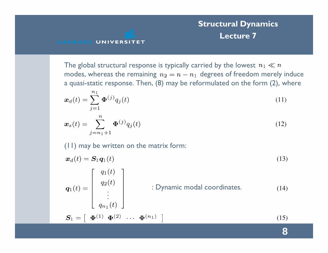
The global structural response is typically carried by the lowest modes, whereas the remaining degrees of freedom merely induce a quasi-static response. Then, (8) may be reformulated on the form (2), where

8

(11) may be written on the matrix form:

: Dynamic modal coordinates.

Structural Dynamics

Lecture 7

Notice that may include both rigid body and elastic degrees of freedom.

Inertial and damping loads may be ignored for the quasi-static modal coordinates, i.e. . Hence, for these degrees of freedom (9) reduces to:

9

Then, (12) may be written as:

Structural Dynamics

Lecture 7

where:

Further, Mercer’s theorem for the flexibility matrix has been used, cf. Lecture 6, Eq. (14):

10

Lecture 6, Eq. (14):

Insertion of (13) and (17) into (2) provides the reduction scheme:

Structural Dynamics

Lecture 7

Hence, and:

The reduction scheme requires that the flexibility matrix is known, along with the eigenmodes and the modal stiffnesses for

. The differential equations (9) for the dynamic modal coordinates may be written on the matrix form:

11

where is given by (18) and:

Structural Dynamics

Lecture 7

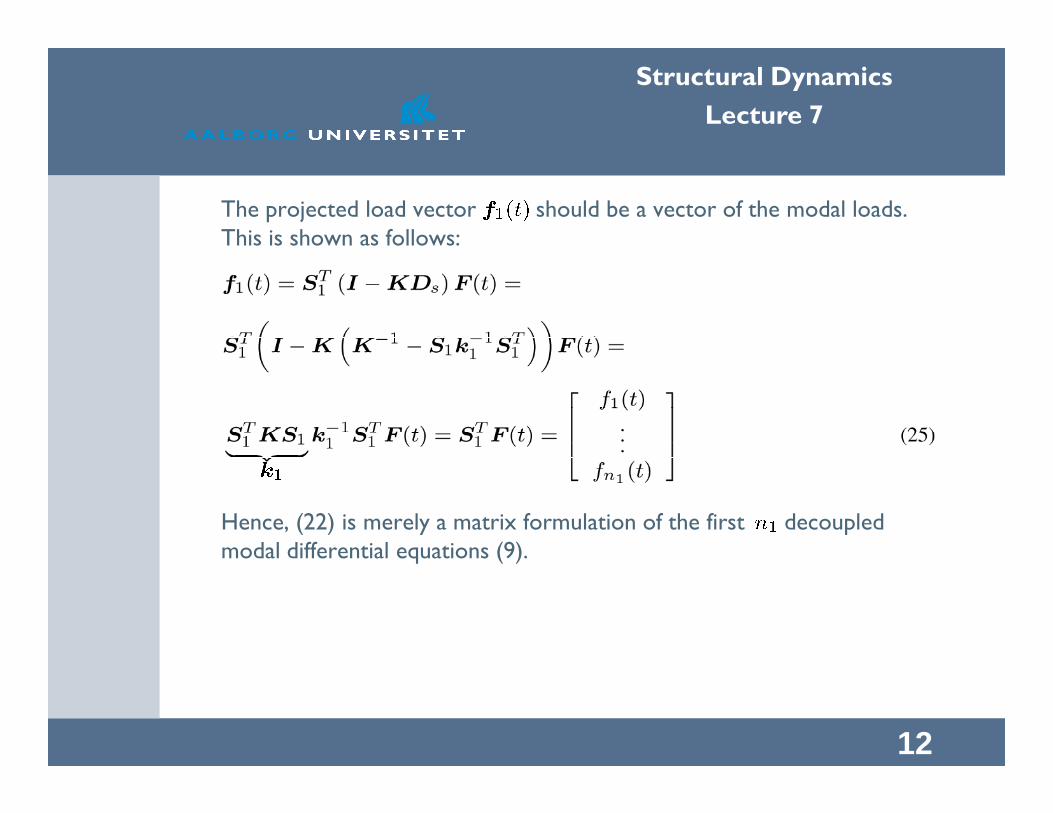
The projected load vector should be a vector of the modal loads. This is shown as follows:

12

Hence, (22) is merely a matrix formulation of the first decoupled modal differential equations (9).

Structural Dynamics

Lecture 7

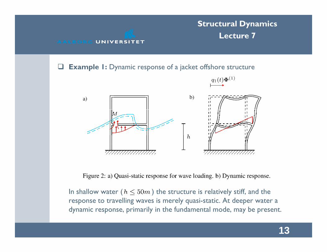
� Example 1: Dynamic response of a jacket offshore structure

13

In shallow water ( ) the structure is relatively stiff, and the response to travelling waves is merely quasi-static. At deeper water a dynamic response, primarily in the fundamental mode, may be present.

Structural Dynamics

Lecture 7

� Guyan Reduction

14

Structural Dynamics

Lecture 7

Guyan has indicated a system reduction scheme, which is based on a partition of the degrees of freedom into two subvectors of the dimension and of the dimension :

The degrees of freedom stored in is presumed to be influenced by

15

The degrees of freedom stored in is presumed to be influenced by inertial, damping, elastic and external dynamic loads. Especially, the kinetic energy of the structure is primarily carried by these degrees of freedom. In contrast, the degrees of freedom stored in are primarily influenced by elastic and external dynamic loads, whereas inertial and damping forces is assumed to be ignorable. Typically, and store displacement and rotational degrees of freedom, respectively, as illustrated for the plane frame structure in Fig. 3a and the plate structure in Fig. 3b.

Structural Dynamics

Lecture 7

Corresponding to the partition (26) the equations of motion (1) are partitioned as:

where , . The quasi-static assumption implies that the lower part of the matrix equation is ignorable affected by inertial

16

that the lower part of the matrix equation is ignorable affected by inertial and damping forces. Hence:

Insertion of (28) into (26) provides the reduction scheme:

Structural Dynamics

Lecture 7

Hence, and:

The projected mass-, damping- and stiffness matrices become:

17

Structural Dynamics

Lecture 7

The projected load vector becomes:

18

Structural Dynamics

Lecture 7

� Vibration due to Movable Supports

19

Structural Dynamics

Lecture 7

The supports of the structure may undergo motions due to earthquakes or heavy traffic. The structural response from such prescribed support motions will be determined.

The degrees of freedom of the structure is partitioned into interior degrees of freedom stored in the vector of dimension , and boundary degrees of freedom stored in the vector of dimension . If mechanical boundary conditions (specified forces or moments) are prescribed at the

20

boundary conditions (specified forces or moments) are prescribed at the boundary, the conjugated displacements and rotations are included in as illustrated for the rotation of the plane frame in Fig. 4.

Eq. (1) may be written on the following partioned form:

Structural Dynamics

Lecture 7

(33) represents the structure of the equations of motion obtained by a FE-analysis in which the global system matrices ( ) have not been corrected for kinematical boundary conditions at the boundary degrees of freedom stored in . and denote the mass matrix, damping matrix and stiffness matrix of the interior degrees of freedom for

. stores the reaction forces acting at the boundary degrees of freedom. Hence, this vector is determined from the last equations in (33) for known and .

21

in (33) for known and .

Then, is determined of the first equations of (33) for known :

Since, , and are assumed to be explicitly known as a function of time, the right-hand side of (34) represents the equivalent dynamic load vector for the determination of the motion of the interior degrees of freedom.

Structural Dynamics

Lecture 7

Often, the inertial and damping loads the right hand side of (34) are ignorable comparable to the elastic load , or disappear completely in cases, where . This provides the so-called quasi-static solution, which may be written on the form:

Let denote the quasi-static displacement vector of the interior

22

Let denote the quasi-static displacement vector of the interior degrees of freedom, where the boundary degrees of freedom are deformed sufficiently slow that no inertial- or damping forces are induced on the left-hand side of (35). It follows from (35) that is given as:

where

Structural Dynamics

Lecture 7

is an influence matrix for the quasi-static support point motion of the dimension . The th column of indicates the quasi-static deformation of for , , , see Fig. 4b. Examples of the calculation of for a three-storey shear building are shown below in Example 2.

Then, the solution to (35) may be decomposed on the form:

23

specifies the dynamic response at the top of the quasi-static contribution , caused by the external load vector and the inertial and damping forces .

Structural Dynamics

Lecture 7

For quasi-static support point motions inducing a rigid body notion on the structure as shown below in Figs. 5a and 5b, may be interpreted as the elastic part of the displacement vector. These are determined by insertion of (38) in (35):

24

where it has been used that cf. (37). Further, a rigid body motion cannot induce dissipation in the structure, so

.

Structural Dynamics

Lecture 7

� Example 2: Determination of the influence matrix for a three-storey building

25

In Fig. 5a the two support points are subjected to the same horizontal .In Fig. 5b the foundation of the structure is rotated the angle as a rigid body. In Fig. 5c the two support points are subjected to different horizontal motions.

Structural Dynamics

Lecture 7

� Earthquake Excitations

26

In earthquake engineering the formulation (39) is preferred. Normally, there is no significant external loading (wind, traffic) present simultaneous with the earthquake loading, so it may assumed . Further, only a common scalar horizontal support point motion is is presumed, so (39) reduces to:

Structural Dynamics

Lecture 7

The influence vector induces a horizontal rigid body motion in all modes. For the three-storey frame in Fig. 6, is given as:

27

The elastic displacement vector may be represented by the following modal expansion:

� : Eigenmodes of interior degrees of freedom for .

Structural Dynamics

Lecture 7

28

Usually, in earthquake engineering the eigenmodes are normalized to for the horizontal displacement of the top storey. Then, the th modal coordinate may be interpreted as the contribution from the th mode to the horizontal displacement of the top storey relative to the ground surface.

Structural Dynamics

Lecture 7

The modal coordinates are assumed to be decoupled. Hence, cf. Lecture 5, Eq. (70):

: Mode partition factor.

29

Save the factor , Eq. (43) has the same form as the differential equation for the relative displacement of a single storey frame exposed to horizontal earthquake excitations, cf. Lecture 3, Eq. (47).

: Mode partition factor.

Structural Dynamics

Lecture 7

Hence, the numerical maximum modal displacement and acceleration of the modal coordinate for a known time series of the ground surface acceleration is given as:

30

and are the spectral displacement and acceleration of the single storey frame calculated with the damping ratio and the angular eigenfrequency , cf. Lecture 3, Eqs. (48) and (50). As mentioned before Eq. (51) in Lecture 3 the relation for

is only approximative.

Structural Dynamics

Lecture 7

The th components of the elastic acceleration vector becomes:

� : Contribution to from the th mode.

� : th component of the th eigenmode .

31

Numerical maximum of :

It is the numerical maximum of , rather than the maxima of the separate modal components , which are of interest. The modal components will not attain their maximum at the same time. Hence, a simple addition of will overestimate unacceptable. Instead, is calculated from

Structural Dynamics

Lecture 7

A theoretical support of (48) is given in stochastic dynamics, where the modal components under certain conditions can be shown to be uncorrelated random variable. The variance of the sum, , becomes equal to the sum of the variance of the components, . Hence:

32

Structural Dynamics

Lecture 7

As explained in Lecture 3 in earthquake resistant design the inertial forcesare next applied as loads on the storey masses as shown in Fig. 8, and

the structure is designed by standard static analysis.

33

Structural Dynamics

Lecture 7

Summary of Lecture 7

� System ReductionGeneral format:

34

: Reduced degrees-of-freedom vector. Dimension: .: Vector base for dynamic subspace. Dimension: .: Flexibility matrix for quasi-static response. Dimension: .

� Truncated Modal Expansion with Quasi-Static Correction.

Structural Dynamics

Lecture 7

: Modal stiffness matrix

35

� Guyan Reduction

Structural Dynamics

Lecture 7

� Vibrations due to Movable SupportsUnsupported structure. The degrees of freedoms are partitioned into interior degrees of freedom and support degrees of freedom :

36

: Dynamic (elastic) degrees of freedom induced by and .

: Quasi-static displacement induced by .

� Earthquake Excitations.

: Quasi-static approximation.