structured belief propagation for nlp matthew r. gormley & jason eisner acl ‘15 tutorial july...
TRANSCRIPT

Structured Belief Propagation for NLP
Matthew R. Gormley & Jason EisnerACL ‘15 TutorialJuly 26, 2015
1For the latest version of these slides, please visit:
http://www.cs.jhu.edu/~mrg/bp-tutorial/

2
Language has a lot going on at once
Structured representations of utterancesStructured knowledge of the language
Many interacting partsfor BP to reason about!

Outline• Do you want to push past the simple NLP models (logistic
regression, PCFG, etc.) that we've all been using for 20 years?• Then this tutorial is extremely practical for you!
1. Models: Factor graphs can express interactions among linguistic structures.
2. Algorithm: BP estimates the global effect of these interactions on each variable, using local computations.
3. Intuitions: What’s going on here? Can we trust BP’s estimates?4. Fancier Models: Hide a whole grammar and dynamic
programming algorithm within a single factor. BP coordinates multiple factors.
5. Tweaked Algorithm: Finish in fewer steps and make the steps faster.
6. Learning: Tune the parameters. Approximately improve the true predictions -- or truly improve the approximate predictions.
7. Software: Build the model you want!
3

Outline• Do you want to push past the simple NLP models (logistic
regression, PCFG, etc.) that we've all been using for 20 years?• Then this tutorial is extremely practical for you!
1. Models: Factor graphs can express interactions among linguistic structures.
2. Algorithm: BP estimates the global effect of these interactions on each variable, using local computations.
3. Intuitions: What’s going on here? Can we trust BP’s estimates?4. Fancier Models: Hide a whole grammar and dynamic
programming algorithm within a single factor. BP coordinates multiple factors.
5. Tweaked Algorithm: Finish in fewer steps and make the steps faster.
6. Learning: Tune the parameters. Approximately improve the true predictions -- or truly improve the approximate predictions.
7. Software: Build the model you want!
4

Outline• Do you want to push past the simple NLP models (logistic
regression, PCFG, etc.) that we've all been using for 20 years?• Then this tutorial is extremely practical for you!
1. Models: Factor graphs can express interactions among linguistic structures.
2. Algorithm: BP estimates the global effect of these interactions on each variable, using local computations.
3. Intuitions: What’s going on here? Can we trust BP’s estimates?4. Fancier Models: Hide a whole grammar and dynamic
programming algorithm within a single factor. BP coordinates multiple factors.
5. Tweaked Algorithm: Finish in fewer steps and make the steps faster.
6. Learning: Tune the parameters. Approximately improve the true predictions -- or truly improve the approximate predictions.
7. Software: Build the model you want!
5

Outline• Do you want to push past the simple NLP models (logistic
regression, PCFG, etc.) that we've all been using for 20 years?• Then this tutorial is extremely practical for you!
1. Models: Factor graphs can express interactions among linguistic structures.
2. Algorithm: BP estimates the global effect of these interactions on each variable, using local computations.
3. Intuitions: What’s going on here? Can we trust BP’s estimates?4. Fancier Models: Hide a whole grammar and dynamic
programming algorithm within a single factor. BP coordinates multiple factors.
5. Tweaked Algorithm: Finish in fewer steps and make the steps faster.
6. Learning: Tune the parameters. Approximately improve the true predictions -- or truly improve the approximate predictions.
7. Software: Build the model you want!
6
Outline• Do you want to push past the simple NLP models (logistic
regression, PCFG, etc.) that we've all been using for 20 years?• Then this tutorial is extremely practical for you!
1. Models: Factor graphs can express interactions among linguistic structures.
2. Algorithm: BP estimates the global effect of these interactions on each variable, using local computations.
3. Intuitions: What’s going on here? Can we trust BP’s estimates?4. Fancier Models: Hide a whole grammar and dynamic
programming algorithm within a single factor. BP coordinates multiple factors.
5. Tweaked Algorithm: Finish in fewer steps and make the steps faster.
6. Learning: Tune the parameters. Approximately improve the true predictions -- or truly improve the approximate predictions.
7. Software: Build the model you want!
7

Outline• Do you want to push past the simple NLP models (logistic
regression, PCFG, etc.) that we've all been using for 20 years?• Then this tutorial is extremely practical for you!
1. Models: Factor graphs can express interactions among linguistic structures.
2. Algorithm: BP estimates the global effect of these interactions on each variable, using local computations.
3. Intuitions: What’s going on here? Can we trust BP’s estimates?4. Fancier Models: Hide a whole grammar and dynamic
programming algorithm within a single factor. BP coordinates multiple factors.
5. Tweaked Algorithm: Finish in fewer steps and make the steps faster.
6. Learning: Tune the parameters. Approximately improve the true predictions -- or truly improve the approximate predictions.
7. Software: Build the model you want!
8
Outline• Do you want to push past the simple NLP models (logistic
regression, PCFG, etc.) that we've all been using for 20 years?• Then this tutorial is extremely practical for you!
1. Models: Factor graphs can express interactions among linguistic structures.
2. Algorithm: BP estimates the global effect of these interactions on each variable, using local computations.
3. Intuitions: What’s going on here? Can we trust BP’s estimates?4. Fancier Models: Hide a whole grammar and dynamic
programming algorithm within a single factor. BP coordinates multiple factors.
5. Tweaked Algorithm: Finish in fewer steps and make the steps faster.
6. Learning: Tune the parameters. Approximately improve the true predictions -- or truly improve the approximate predictions.
7. Software: Build the model you want!
9
Outline• Do you want to push past the simple NLP models (logistic
regression, PCFG, etc.) that we've all been using for 20 years?• Then this tutorial is extremely practical for you!
1. Models: Factor graphs can express interactions among linguistic structures.
2. Algorithm: BP estimates the global effect of these interactions on each variable, using local computations.
3. Intuitions: What’s going on here? Can we trust BP’s estimates?4. Fancier Models: Hide a whole grammar and dynamic
programming algorithm within a single factor. BP coordinates multiple factors.
5. Tweaked Algorithm: Finish in fewer steps and make the steps faster.
6. Learning: Tune the parameters. Approximately improve the true predictions -- or truly improve the approximate predictions.
7. Software: Build the model you want!
10

Section 1:Introduction
Modeling with Factor Graphs
11
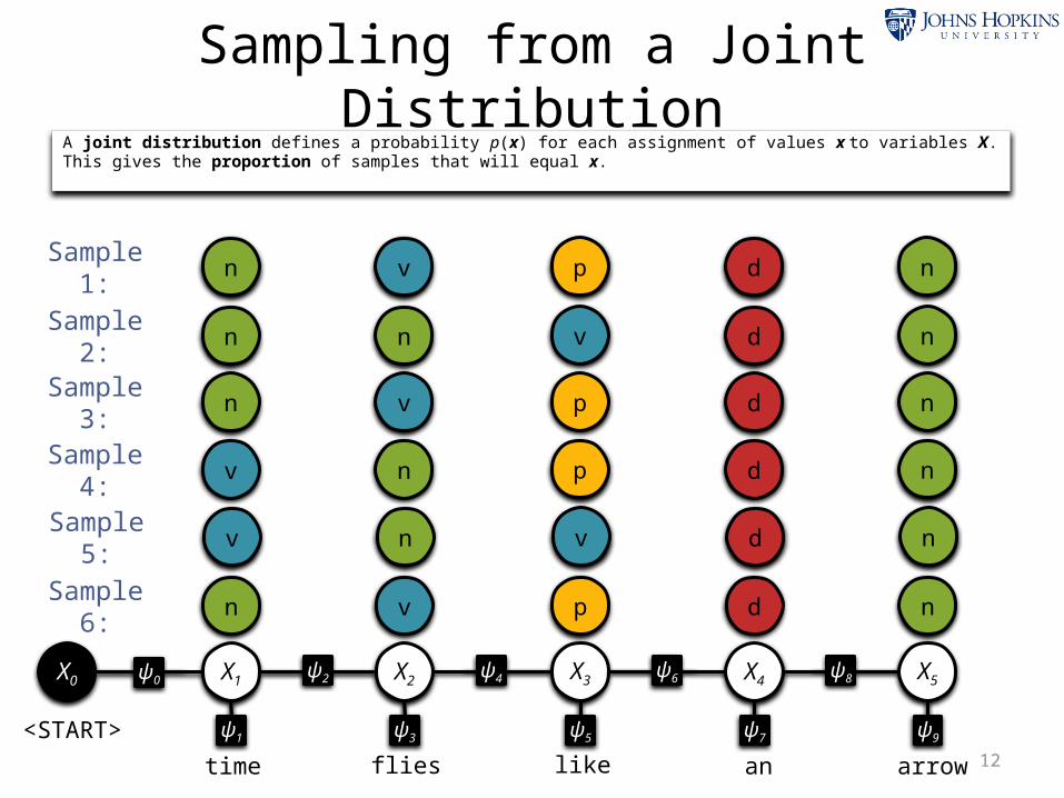
Sampling from a Joint Distribution
12time likeflies an arrow
X1ψ2 X2
ψ4 X3ψ6 X4
ψ8 X5
ψ1 ψ3 ψ5 ψ7 ψ9
ψ0X0
<START>
n v p d nSample
6:
v n v d nSample
5:
v n p d nSample
4:
n v p d nSample
3:
n n v d nSample
2:
n v p d nSample
1:
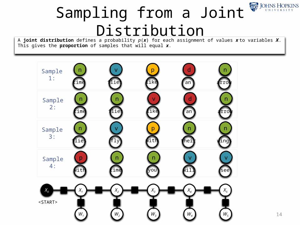
A joint distribution defines a probability p(x) for each assignment of values x to variables X. This gives the proportion of samples that will equal x.

Sampling from a Joint Distribution
13
X1
ψ1
ψ2
X2
ψ3
ψ4
X3
ψ5
ψ6
X4
ψ7
ψ8
X5
ψ9
X6
ψ10
X7
ψ12
ψ11
Sample 1:
ψ1
ψ2
ψ3
ψ4
ψ5
ψ6
ψ7
ψ8
ψ9
ψ10
ψ12
ψ11
Sample 2:
ψ1
ψ2
ψ3
ψ4
ψ5
ψ6
ψ7
ψ8
ψ9
ψ10
ψ12
ψ11
Sample 3:
ψ1
ψ2
ψ3
ψ4
ψ5
ψ6
ψ7
ψ8
ψ9
ψ10
ψ12
ψ11
Sample 4:
ψ1
ψ2
ψ3
ψ4
ψ5
ψ6
ψ7
ψ8
ψ9
ψ10
ψ12
ψ11
A joint distribution defines a probability p(x) for each assignment of values x to variables X. This gives the proportion of samples that will equal x.
n n v d nSample 2:
time likeflies an arrow
Sampling from a Joint Distribution
14W1 W2 W3 W4 W5
X1 ψ2 X2 ψ4 X3 ψ6 X4 ψ8 X5
ψ1 ψ3 ψ5 ψ7 ψ9
ψ0X0
<START>
n v p d nSample 1:
time likeflies an arrow
p n n v vSample 4:
with youtime will see
n v p n nSample 3:
flies withfly their wings
A joint distribution defines a probability p(x) for each assignment of values x to variables X. This gives the proportion of samples that will equal x.

W1 W2 W3 W4 W5
X1 ψ2 X2 ψ4 X3 ψ6 X4 ψ8 X5
ψ1 ψ3 ψ5 ψ7 ψ9
ψ0X0
<START>
Factors have local opinions (≥ 0)
15
Each black box looks at some of the tags Xi and words Wi
v n p dv 1 6 3 4
n 8 4 2 0.1
p 1 3 1 3
d 0.1 8 0 0
v n p dv 1 6 3 4
n 8 4 2 0.1
p 1 3 1 3
d 0.1 8 0 0
time
flies
like …
v 3 5 3n 4 5 2
p 0.1
0.1 3
d 0.1
0.2
0.1
time
flies
like …
v 3 5 3n 4 5 2
p 0.1
0.1 3
d 0.1
0.2
0.1
Note: We chose to reuse the same factors at
different positions in the sentence.

Factors have local opinions (≥ 0)
16
time flies like an arrow
n ψ2 v ψ4 p ψ6 d ψ8 n
ψ1 ψ3 ψ5 ψ7 ψ9
ψ0<START>
Each black box looks at some of the tags Xi and words Wi
v n p dv 1 6 3 4
n 8 4 2 0.1
p 1 3 1 3
d 0.1 8 0 0
v n p dv 1 6 3 4
n 8 4 2 0.1
p 1 3 1 3
d 0.1 8 0 0
time
flies
like …
v 3 5 3n 4 5 2
p 0.1
0.1 3
d 0.1
0.2
0.1
time
flies
like …
v 3 5 3n 4 5 2
p 0.1
0.1 3
d 0.1
0.2
0.1
p(n, v, p, d, n, time, flies, like, an, arrow) = ?

Global probability = product of local opinions
17
time flies like an arrow
n ψ2 v ψ4 p ψ6 d ψ8 n
ψ1 ψ3 ψ5 ψ7 ψ9
ψ0<START>
Each black box looks at some of the tags Xi and words Wi
p(n, v, p, d, n, time, flies, like, an, arrow) = (4 * 8 * 5 * 3 * …)
v n p dv 1 6 3 4
n 8 4 2 0.1
p 1 3 1 3
d 0.1 8 0 0
v n p dv 1 6 3 4
n 8 4 2 0.1
p 1 3 1 3
d 0.1 8 0 0
time
flies
like …
v 3 5 3n 4 5 2
p 0.1
0.1 3
d 0.1
0.2
0.1
time
flies
like …
v 3 5 3n 4 5 2
p 0.1
0.1 3
d 0.1
0.2
0.1
Uh-oh! The probabilities of the various assignments
sum up to Z > 1.So divide them all by Z.
Markov Random Field (MRF)
18
time flies like an arrow
n ψ2 v ψ4 p ψ6 d ψ8 n
ψ1 ψ3 ψ5 ψ7 ψ9
ψ0<START>
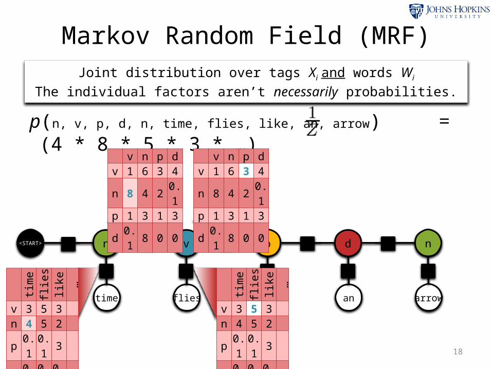
p(n, v, p, d, n, time, flies, like, an, arrow) = (4 * 8 * 5 * 3 * …)
v n p dv 1 6 3 4
n 8 4 2 0.1
p 1 3 1 3
d 0.1 8 0 0
v n p dv 1 6 3 4
n 8 4 2 0.1
p 1 3 1 3
d 0.1 8 0 0
time
flies
like …
v 3 5 3n 4 5 2
p 0.1
0.1 3
d 0.1
0.2
0.1
time
flies
like …
v 3 5 3n 4 5 2
p 0.1
0.1 3
d 0.1
0.2
0.1
Joint distribution over tags Xi and words Wi
The individual factors aren’t necessarily probabilities.

time flies like an arrow
n v p d n<START>
Hidden Markov Model
19
But sometimes we choose to make them probabilities. Constrain each row of a factor to sum to one. Now Z = 1.
v n p dv .1 .4 .2 .3n .8 .1 .1 0p .2 .3 .2 .3d .2 .8 0 0
v n p dv .1 .4 .2 .3n .8 .1 .1 0p .2 .3 .2 .3d .2 .8 0 0
time
flies
like …
v .2 .5 .2n .3 .4 .2p .1 .1 .3d .1 .2 .1
time
flies
like …
v .2 .5 .2n .3 .4 .2p .1 .1 .3d .1 .2 .1
p(n, v, p, d, n, time, flies, like, an, arrow) = (.3 * .8 * .2 * .5 * …)
Markov Random Field (MRF)
20
time flies like an arrow
n ψ2 v ψ4 p ψ6 d ψ8 n
ψ1 ψ3 ψ5 ψ7 ψ9
ψ0<START>
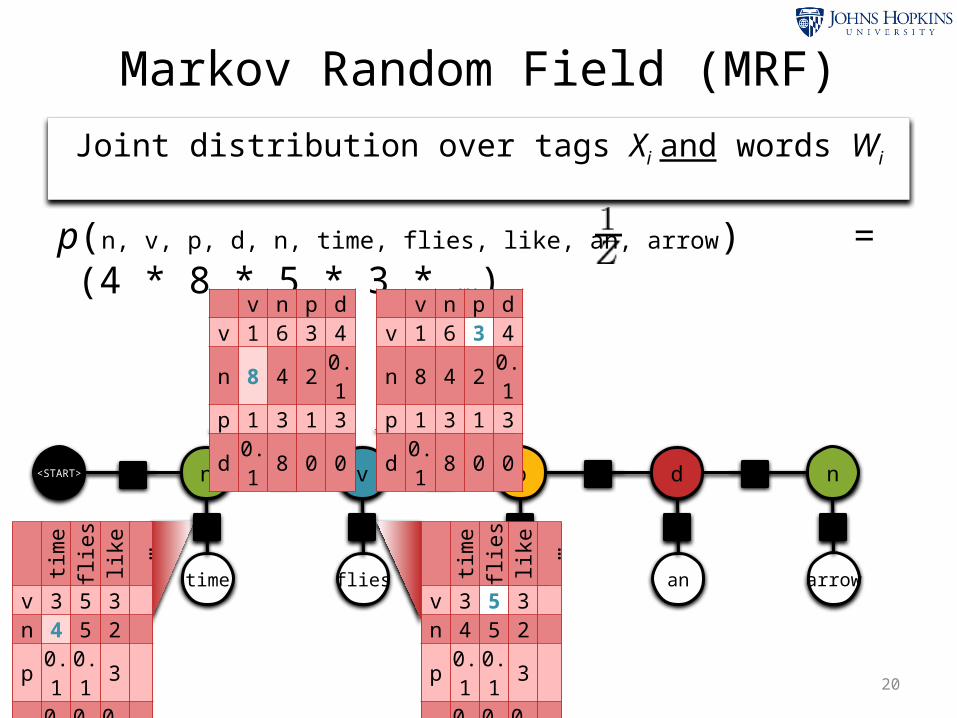
p(n, v, p, d, n, time, flies, like, an, arrow) = (4 * 8 * 5 * 3 * …)
v n p dv 1 6 3 4
n 8 4 2 0.1
p 1 3 1 3
d 0.1 8 0 0
v n p dv 1 6 3 4
n 8 4 2 0.1
p 1 3 1 3
d 0.1 8 0 0
time
flies
like …
v 3 5 3n 4 5 2
p 0.1
0.1 3
d 0.1
0.2
0.1
time
flies
like …
v 3 5 3n 4 5 2
p 0.1
0.1 3
d 0.1
0.2
0.1
Joint distribution over tags Xi and words Wi
Conditional Random Field (CRF)
21time flies like an arrow
n ψ2 v ψ4 p ψ6 d ψ8 n
ψ1 ψ3 ψ5 ψ7 ψ9
ψ0<START>
v 3n 4
p 0.1
d 0.1
v n p dv 1 6 3 4
n 8 4 2 0.1
p 1 3 1 3
d 0.1 8 0 0
v n p dv 1 6 3 4
n 8 4 2 0.1
p 1 3 1 3
d 0.1 8 0 0
v 5n 5
p 0.1
d 0.2
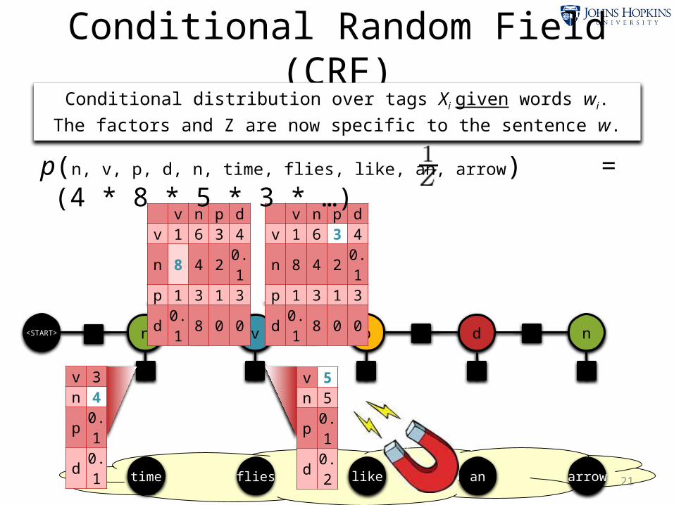
Conditional distribution over tags Xi given words wi.The factors and Z are now specific to the sentence w.
p(n, v, p, d, n, time, flies, like, an, arrow) = (4 * 8 * 5 * 3 * …)

How General Are Factor Graphs?
• Factor graphs can be used to describe–Markov Random Fields (undirected graphical
models)• i.e., log-linear models over a tuple of variables
– Conditional Random Fields– Bayesian Networks (directed graphical models)
• Inference treats all of these interchangeably.– Convert your model to a factor graph first.– Pearl (1988) gave key strategies for exact
inference:• Belief propagation, for inference on acyclic
graphs• Junction tree algorithm, for making any
graph acyclic(by merging variables and factors: blows up the runtime)
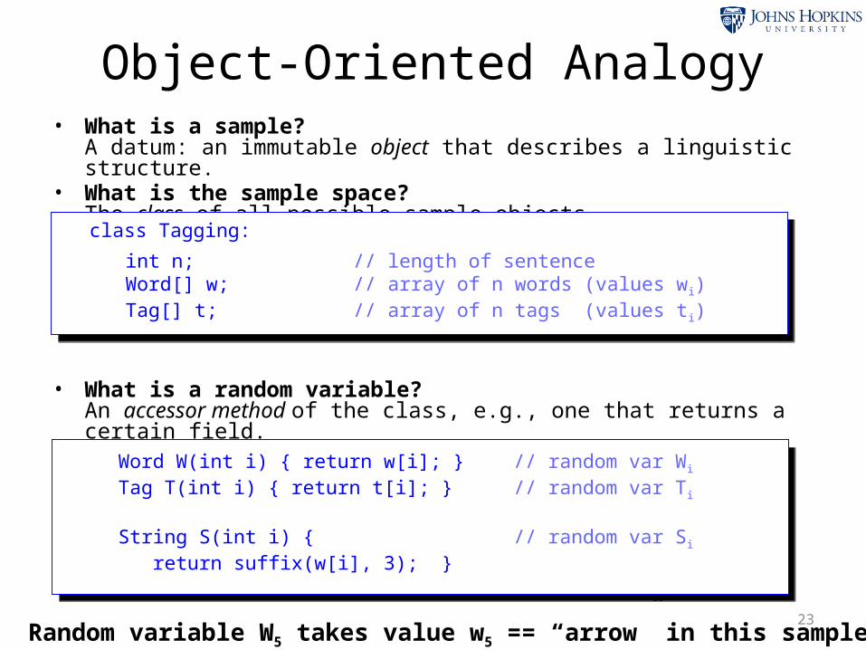
Object-Oriented Analogy• What is a sample?
A datum: an immutable object that describes a linguistic structure.
• What is the sample space?The class of all possible sample objects.
• What is a random variable? An accessor method of the class, e.g., one that returns a certain field.– Will give different values when called on different random
samples.
23
class Tagging:
int n; // length of sentenceWord[] w; // array of n words (values wi)Tag[] t; // array of n tags (values ti)
Word W(int i) { return w[i]; } // random var Wi
Tag T(int i) { return t[i]; } // random var Ti
String S(int i) { // random var Si
return suffix(w[i], 3); }
Random variable W5 takes value w5 == “arrow” in this sample
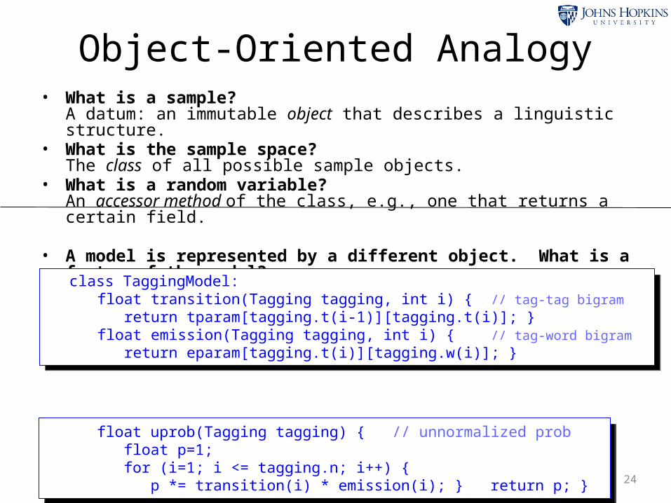
Object-Oriented Analogy• What is a sample?
A datum: an immutable object that describes a linguistic structure.• What is the sample space?
The class of all possible sample objects.• What is a random variable?
An accessor method of the class, e.g., one that returns a certain field.
• A model is represented by a different object. What is a factor of the model?A method of the model that computes a number ≥ 0 from a sample, based on the sample’s values of a few random variables, and parameters stored in the model.
• What probability does the model assign to a sample? A product of its factors (rescaled). E.g., uprob(tagging) / Z().
• How do you find the scaling factor? Add up the probabilities of all possible samples. If the result Z != 1, divide the probabilities by that Z.
24
class TaggingModel:float transition(Tagging tagging, int i) { // tag-tag bigram return tparam[tagging.t(i-1)][tagging.t(i)]; }float emission(Tagging tagging, int i) { // tag-word bigram return eparam[tagging.t(i)][tagging.w(i)]; }
float uprob(Tagging tagging) { // unnormalized prob float p=1; for (i=1; i <= tagging.n; i++) { p *= transition(i) * emission(i); } return p; }

Modeling with Factor Graphs• Factor graphs can be used to
model many linguistic structures.
• Here we highlight a few example NLP tasks.– People have used BP for all of these.
• We’ll describe how variables and factors were used to describe structures and the interactions among their parts.
25

Annotating a Tree
26
Given: a sentence and unlabeled parse tree.
n v p d n
time likeflies an arrow
np
vp
pp
s
Annotating a Tree
27
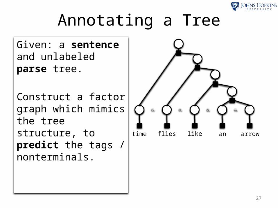
Given: a sentence and unlabeled parse tree.
Construct a factor graph which mimics the tree structure, to predict the tags / nonterminals.
X1
ψ1
ψ2 X2
ψ3
ψ4 X3
ψ5
ψ6 X4
ψ7
ψ8 X5
ψ9
time likeflies an arrow
X6
ψ10
X8
ψ12
X7
ψ11
X9
ψ13

Annotating a Tree
28
Given: a sentence and unlabeled parse tree.
Construct a factor graph which mimics the tree structure, to predict the tags / nonterminals.
n
ψ1
ψ2 v
ψ3
ψ4 p
ψ5
ψ6 d
ψ7
ψ8 n
ψ9
time likeflies an arrow
npψ10
vpψ12
ppψ11
sψ13
Annotating a Tree
29
n
ψ1
ψ2 v
ψ3
ψ4 p
ψ5
ψ6 d
ψ7
ψ8 n
ψ9
time likeflies an arrow
npψ10
vpψ12
ppψ11
sψ13
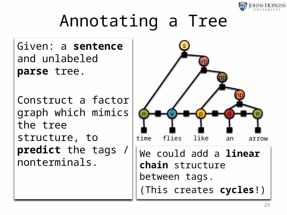
Given: a sentence and unlabeled parse tree.
Construct a factor graph which mimics the tree structure, to predict the tags / nonterminals. We could add a linear
chain structure between tags.(This creates cycles!)

Constituency Parsing
30
n
ψ1
ψ2 v
ψ3
ψ4 p
ψ5
ψ6 d
ψ7
ψ8 n
ψ9
time likeflies an arrow
npψ10
vpψ12
ppψ11
sψ13
What if we needed to predict the tree structure too?
Use more variables: Predict the nonterminal of each substring, or ∅ if it’s not a constituent.
∅ψ10
∅ψ10
∅ψ10
∅ψ10
∅ψ10
∅ψ10

Constituency Parsing
31
n
ψ1
ψ2 v
ψ3
ψ4 p
ψ5
ψ6 d
ψ7
ψ8 n
ψ9
time likeflies an arrow
npψ10
vpψ12
ppψ11
sψ13
What if we needed to predict the tree structure too?
Use more variables: Predict the nonterminal of each substring, or ∅ if it’s not a constituent.
But nothing prevents non-tree structures.
∅ψ10
∅ψ10
sψ10
∅ψ10
∅ψ10
∅ψ10

Constituency Parsing
32
n
ψ1
ψ2 v
ψ3
ψ4 p
ψ5
ψ6 d
ψ7
ψ8 n
ψ9
time likeflies an arrow
npψ10
vpψ12
ppψ11
sψ13
What if we needed to predict the tree structure too?
Use more variables: Predict the nonterminal of each substring, or ∅ if it’s not a constituent.
But nothing prevents non-tree structures.
∅ψ10
∅ψ10
sψ10
∅ψ10
∅ψ10
∅ψ10

Constituency Parsing
33
n
ψ1
ψ2 v
ψ3
ψ4 p
ψ5
ψ6 d
ψ7
ψ8 n
ψ9
time likeflies an arrow
npψ10
vpψ12
ppψ11
sψ13
What if we needed to predict the tree structure too?
Use more variables: Predict the nonterminal of each substring, or ∅ if it’s not a constituent.
But nothing prevents non-tree structures.
∅ψ10
∅ψ10
sψ10
∅ψ10
∅ψ10
∅ψ10
Add a factor which multiplies in 1 if the variables form a tree and 0 otherwise.

Constituency Parsing
34
n
ψ1
ψ2 v
ψ3
ψ4 p
ψ5
ψ6 d
ψ7
ψ8 n
ψ9
time likeflies an arrow
npψ10
vpψ12
ppψ11
sψ13
What if we needed to predict the tree structure too?
Use more variables: Predict the nonterminal of each substring, or ∅ if it’s not a constituent.
But nothing prevents non-tree structures.
∅ψ10
∅ψ10
∅ψ10
∅ψ10
∅ψ10
∅ψ10
Add a factor which multiplies in 1 if the variables form a tree and 0 otherwise.

Constituency Parsing• Variables: – Constituent type
(or ∅) for each of O(n2) substrings
• Interactions:– Constituents must
describe a binary tree
– Tag bigrams– Nonterminal triples
(parent, left-child, right-child) [these factors not shown]
35
Example Task:
(Naradowsky, Vieira, & Smith, 2012)
n v p d n
time likeflies an arrow
np
vp
pp
s
n
ψ1
ψ2 v
ψ3
ψ4 p
ψ5
ψ6 d
ψ7
ψ8 n
ψ9
time likeflies an arrow
np
ψ10
vp
ψ12
pp
ψ11
s
ψ13
∅
ψ10
∅
ψ10
∅
ψ10
∅
ψ10
∅
ψ10
∅
ψ10

Dependency Parsing• Variables: – POS tag for each
word– Syntactic label (or
∅) for each of O(n2) possible directed arcs
• Interactions: – Arcs must form a
tree– Discourage (or
forbid) crossing edges
– Features on edge pairs that share a vertex
36(Smith & Eisner, 2008)
Example Task:
time likeflies an arrow
*Figure from Burkett & Klein (2012)
• Learn to discourage a verb from having 2 objects, etc.
• Learn to encourage specific multi-arc constructions

Joint CCG Parsing and Supertagging
• Variables:– Spans– Labels on non-
terminals– Supertags on pre-
terminals
• Interactions:– Spans must form a
tree– Triples of labels:
parent, left-child, and right-child
– Adjacent tags37
(Auli & Lopez, 2011)
Example Task:
38Figure thanks to Markus
Dreyer
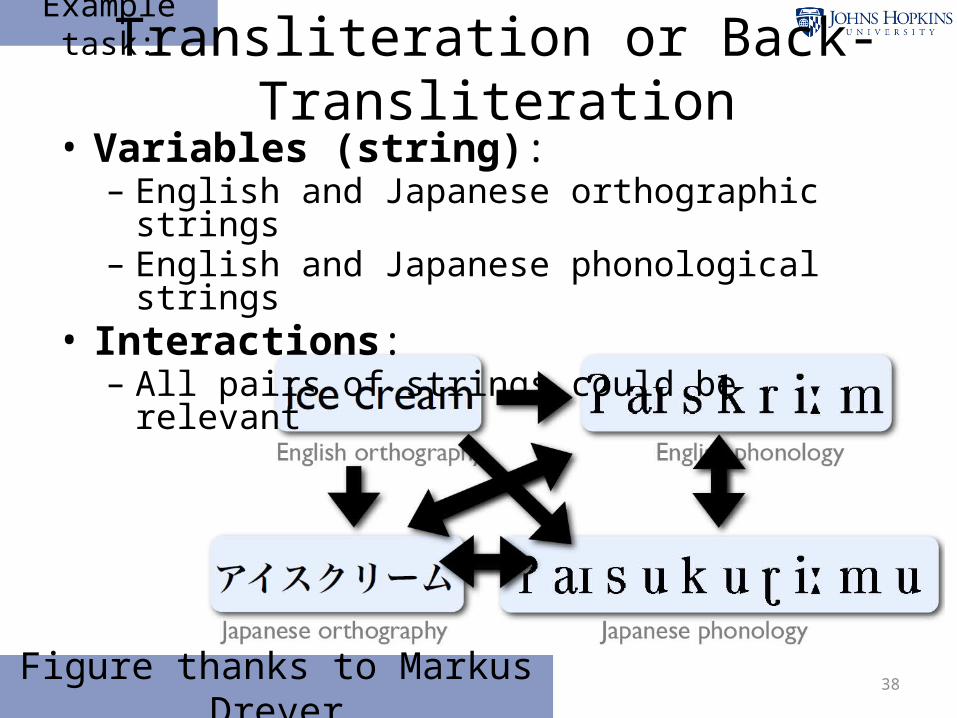
Example task: Transliteration or Back-
Transliteration• Variables (string):– English and Japanese orthographic
strings– English and Japanese phonological
strings• Interactions:– All pairs of strings could be relevant
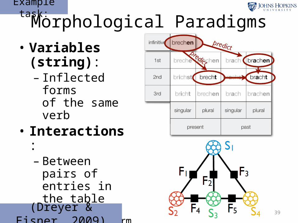
• Variables (string): – Inflected forms
of the same verb
• Interactions: – Between pairs
of entries in the table (e.g. infinitive form affects present-singular)
39(Dreyer & Eisner,
2009)
Example task:
Morphological Paradigms
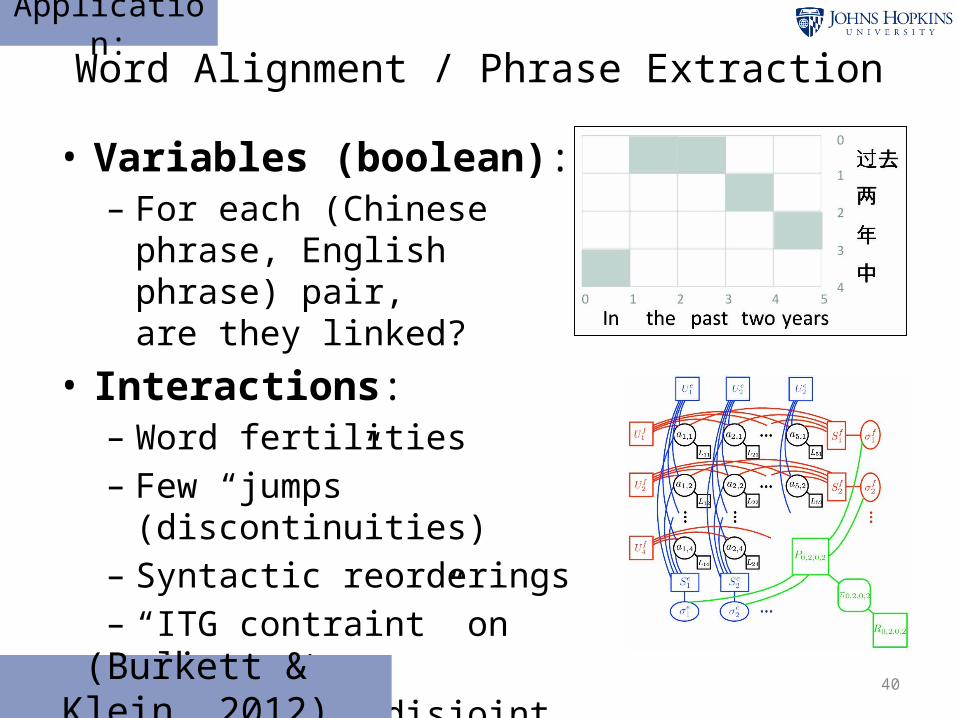
Word Alignment / Phrase Extraction
• Variables (boolean):– For each (Chinese
phrase, English phrase) pair, are they linked?
• Interactions:– Word fertilities– Few “jumps”
(discontinuities)– Syntactic reorderings– “ITG contraint” on
alignment– Phrases are disjoint (?)
40(Burkett & Klein,
2012)
Application:

Congressional Voting
41(Stoyanov & Eisner,
2012)
Application:
• Variables:– Representative’s vote– Text of all speeches of a
representative – Local contexts of
references between two representatives
• Interactions:– Words used by
representative and their vote
– Pairs of representatives and their local context

Semantic Role Labeling with Latent Syntax
• Variables:– Semantic predicate
sense– Semantic dependency
arcs– Labels of semantic arcs– Latent syntactic
dependency arcs
• Interactions:– Pairs of syntactic and
semantic dependencies– Syntactic dependency
arcs must form a tree
42
(Naradowsky, Riedel, & Smith, 2012) (Gormley, Mitchell, Van Durme, & Dredze, 2014)
Application:
time likeflies an arrow
arg0arg1
0 21 3 4The madebarista coffee<WALL>
R2,1
L2,1
R1,2
L1,2
R3,2
L3,2
R2,3
L2,3
R3,1
L3,1
R1,3
L1,3
R4,3
L4,3
R3,4
L3,4
R4,2
L4,2
R2,4
L2,4
R4,1
L4,1
R1,4
L1,4
L0,1
L0,3
L0,4
L0,2
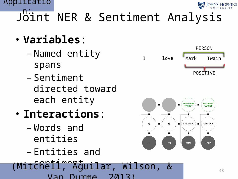
Joint NER & Sentiment Analysis
• Variables:– Named entity
spans– Sentiment
directed toward each entity
• Interactions:–Words and
entities– Entities and
sentiment43
(Mitchell, Aguilar, Wilson, & Van Durme, 2013)
Application:
loveI Mark Twain
PERSON
POSITIVE

44
Variable-centric view of the world
When we deeply understand language, what representations (type and token) does that understanding comprise?

45
lexicon (word types)semantics
sentences
discourse context
resources
entailmentcorrelation
inflectioncognatestransliterationabbreviationneologismlanguage evolution
translationalignment
editingquotation
speech misspellings,typos formatting entanglement annotation
N
tokens
To recover variables, model and exploit their correlations