Department of Electronic Engineering

FINAL YEAR PROJECT REPORT

BEngCE-2008/09-KLC-03

Human Motion Analysis

Student Name: Chu Kwong Wai Student ID: Supervisor: Dr. CHAN, K L Assessor: Dr. CHAN, Stanley C F

Bachelor of Engineering (Honours) in Computer Engineering

Student Final Year Project Declaration

I have read the student handbook and I understand the meaning of academic dishonesty, in particular plagiarism and collusion. I declare that the work submitted for the final year project does not involve academic dishonesty. I give permission for my final year project work to be electronically scanned and if found to involve academic dishonesty, I am aware of the consequences as stated in the Student Handbook. Project Title : Human Motion Analysis

Student Name : Chu Kwong Wai

Student ID:

Signature

Date : 23-Apr-09

No part of this report may be reproduced, stored in a retrieval system, or transcribed in any form or by any means – electronic, mechanical, photocopying, recording or otherwise – without the prior written permission of City University of Hong Kong.

i

Table of Contents:

List of Figures……………………………………………. iii

Abstract…………………………………………………… v

Chapter 1 Introduction………………………………… 1

1.1 Background………………………………………………… 1

1.2 Objectives………………………………………………….. 3

1.3 Challenges Faced………………………………………….. 3

1.4 Chapter Outline……………………………………………. 5

Chapter 2 Related Work………………………………… 6

2.1 Background Subtraction…………………………………… 6

2.2 Skeletonization…………………………………………….. 6

2.3 Motion Tracking…………………………………………… 7

Chapter 3 Methodology………………………………… 9

3.1 System Overview………………………………………….. 9

3.2 Background Subtraction Module………………………….. 11

3.2.1 Background Modeling…………………………… 11

3.2.2 K-means Algorithm……………………………… 13

3.2.3 Foreground Detection……………………………. 14

3.2.4 Median Filter…………………………………….. 16

ii

3.3 Analysis Module…………………………………………. 18

3.3.1 Dilation Operation……………………................. 18

3.3.2 Erosion Operation………………………………. 21

3.3.3 Boundary Extraction……………………………. 23

3.3.4 Removing the Non-body Objects………………. 25

3.3.5 Extracting Extremal Points……………………... 28

3.3.6 Locating Interested Points……………………… 30

3.4 Tracking Module………………………………………… 33

Chapter 4 Result……………………………………... 35

4.1 System Configuration……………………………………… 35

4.2 Background Subtraction……………………………………. 36

4.3 Median Filter………………………………………………... 39

4.4 Morphological Operations………………………………….. 40

4.5 Locating Interested Points…………………………………... 42

4.6 Tracking Process…………………………………………….. 43

4.6.1 Result of Kalman Filter……………………………… 43

4.6.2 Object Tracking………………………………………. 45

Chapter 5 Discussion…………………………………… 47

Chapter 6 Conclusion…………………………………... 50

Reference…………………………………………………… 51

iii

List of Figures

Figure 1. Flow chart of human motion analysis system……………………… 9

Figure 2. Demonstration of a region based background modeling process….. 11

Figure 3. Modeling composite background………………………………….. 12

Figure 4. Flow chart of the K-means algorithm employed………………….. 13

Figure 5. Histogram of an image block with two background regions……… 14

Figure 6. Results of background subtraction & median filtering…………… 16

Figure 7. Calculating the median value of a pixel neighborhood………….. . 17

Figure 8. Result of dilation operation………………………………………. 19

Figure 9. 8-connected neighborhood……………………………………….. 20

Figure 10. Illustration of dilation operation………………………………… 20

Figure 11. Result of erosion operation……………………………………… 22

Figure 12. Illustration of erosion operation…………………………………. 22

Figure 13. Result of boundary extraction…………………………………… 23

Figure 14. Illustration of boundary extraction operation…………………… 24

Figure 15. Removal of non-body objects…………………………………… 25

Figure 16. Connected component labeling………………………………...... 27

Figure 17. Process of extracting extremal points……………………………. 28

Figure 18. Interested points located…………………………………………. 30

Figure 19. Locating elbow position……………………………………….... 31

Figure 20. Locating shoulder position………………………………………. 32

Figure 21. Illustration of Kalman filter……………………………………… 33

Figure 22. Results of background subtraction……………………………..... 36

Figure 23. Comparison between frame difference & region-based approach.. 37

Figure 24. Median filtering…………………………………………………... 39

iv

Figure 25. Two sets of results of morphological operations…………………. 41

Figure 26. Located interested points…………………………………………. 42

Figure 27. An unsuccessful case on locating interested points………………. 42

Figure 28. Result of tracking of the centroid of swimmer…………………… 43

Figure 29. Applying Kalman filter on tracking interested points…………….. 44

Figure 30. Object tracking……………………………………………………. 45

v

Abstract

This project aims to analyze human motion in an image sequence of swimming. The

proposed system consists of three main modules. First, a background subtraction

module segments the human region in spite of large scene variations in the monitored

pool areas. Second, the analysis module obtains the skeletonization of the segmented

region of human. Finally, a tracking module is used to acquire the trajectories of the

body parts. The background subtraction module employs a region-based background

modeling approach that can differentiate the moving human subject from the

nonstationary water surface. The skeletonization is obtained by locating the interested

points such as hands, elbows and shoulders of the human. The tracking module

utilizes the Kalman filter to find the position of the human body and the trajectories of

the body parts. We test the human motion analysis system using video clips of

breaststroke swimming. The experimental results are very good.

- 1 -

Chapter 1 Introduction

1.1 Background

Human motion analysis has been an active research topic in computer vision for

decades. This research topic aims at developing a system which can understand

human activities; such system would be an essential part of many applications such as

human-robot interaction, sports video analysis and visual surveillance. For instance,

human motion analysis enables a robot to understand the motion of human, which is

very important for having an effective communication between robot and human.

Triesch and von der Malsburg [1] proposed a mechanism for implementing a gesture

interface for human-robot interaction, which enables a robot to understand simple

gesture commands from human such as grasping and moving objects. It is believable

that more natural and intelligent communication between human and robot could be

achieved in the future. In the application of sports, human motion analysis system can

segment different parts of the human body, track the trajectories of various joints over

an image sequence, and reconstruct the 3-D human body structure. Those are

particular useful information for the coaches to analyze the performance of athletes,

and study the motions which cause injuries. Human motion analysis system is also

- 2 -

often seen in the automatic visual surveillance, which aims to perform monitoring

tasks automatically in order to improve the safety in different environment. For

example, [2] provides commercial products of automatic video surveillance system,

which can detect, record and transmit various kinds of motion activity. Besides, Eng

et al. [3] developed a live visual surveillance system for detecting early drowning at

swimming pool, which is definitely able to increase the quality of work of the

lifeguards.

Human motion analysis is the preprocessing step of human motion recognition,

because before any recognition process could be performed on the human body, a

variety of information of the body part must be obtained by the human motion

analysis process. Traditionally, the work of human motion analysis could be divided

into the following parts: 1) segmenting the human body part from video frames using

background subtraction approach, which usually need to build up a background model;

2) locating some interested joints on the human body part, which often makes use of

prior information or employs 2D or 3D human model; 3) tracking the movement of

the human body, which relies on the correspondence of image features between

consecutive video frames with the information of human body part’s position, shape

and velocity.

- 3 -

1.2 Objectives

In this report we address the problem of developing a system for analyzing and

tracking the motion of swimmers at the pool. The final year project has the following

the objectives:

˙Obtain the body part region of the swimmer from an image sequence of a

swimming video.

˙Locate some interested points on the upper parts of the human body.

˙Track the human body along the image sequence in order to get the

trajectories of swimmer.

1.3 Challenges Faced

One key challenge we faced during the project development is the relatively high

level of noise in human body part segmentation. It is because performing background

subtraction on video of an aquatic environment is much more complex than doing that

on video of the terrestrial scene. In the aquatic environment, the water surface is keep

fluctuating, which contributes to a non-stationary background for the background

subtraction process. The intensity variation of pixels at the scene over time is in a very

wide distribution, which is demonstrated in Figure 1 of [4]. The background

subtraction could not be done with traditional frame difference approach, which

- 4 -

differentiates the foreground objects from background based on the intensity

difference of pixels in the foreground and background images. In our system, we use a

region-based approach for the background subtraction, which would be less sensitive

to the wide intensity change over video frames. Further discussion would be provided

in the methodology chapter.

Apart from the above problem in background subtraction, there are also problems

existing in locating features and tracking. Some feature points such as the hands will

be relatively easier to locate since they are the most outstanding part of the body. By

locating the extremal points on the boundary of the human body can successfully

locate the hands position, which will be discussed in the methodology chapter.

Nevertheless, the other feature points such as shoulders and elbows will be much

more difficult to locate since they have not apparent characteristic like the hands.

Sometimes those feature points will be covered by the water or cannot be

differentiated from the body part, which makes the locating process even harder.

Using a predefined ratio between those feature points can help the locating process

and that will be discussed in the methodology chapter.

For the tracking process, the major problem is that sometimes the measurement data

- 5 -

will be missing due to the background subtraction process, which will affect the

tracking performance. A discussion about this issue will be provided in the result of

the tracking process in the result chapter.

1.4 Chapter Outline

This report is organized as follow. In Chapter 2, we review relevant prior works on

human motion analysis, which mainly focuses on background subtraction,

skeletonization of the extracted human region and motion tracking. Chapter 3 gives a

detailed explanation on the methodologies employed for the analysis system. In

chapter 4, experiment results of each stage of the human motion analysis are provided.

Finally, discussion and conclusion are presented in chapter 5 and 6 respectively.

- 6 -

Chapter 2 Related Work

2.1 Background Subtraction

In order to handle the highly dynamic aquatic background, Eng et al. [4] proposed a

homogeneous region-based modeling approach for background subtraction. This

approach takes the background as a composition of homogeneous region processes. A

sequence of background frames is needed to form the homogeneous background

region. For each of these background frames, it would be first divided into a number

of non-overlapping square blocks. Then, a hierarchical K-means algorithm is

performed on color vectors collected from these divided square blocks to form

homogeneous regions. This approach enables an efficient spatial searching scheme

with long-range spatial displacement search ability to capture the background pixels

movements. However, an additional devised thresholding scheme is needed in the

foreground detection process in order to have efficient result.

2.2 Skeletonization

Fujiyoshi and Lipton [5] proposed a real-time, robust and computational cheap

approach to get a “star” skeleton of a human target. This approach first detects

moving targets and extracts their boundaries. Each skeleton is obtained by detecting

- 7 -

and extracting the extremal points on the boundary of the segmented target object.

The “star” skeleton has only the extremals of the target object jointed to its centroid

point. The “star” skeleton can be used to determine the body posture and cyclic

motion of body segments, which are useful cues for analyzing human activities such

as walking and running. Since this approach is not iterative, so it is computational

inexpensive. It also provides a mechanism for controlling scale sensitivity.

Nevertheless, it does not rely on any priori human model; therefore it is very useful

for real-time application. However, this “star” skeleton consists of only the extremal

points such as hands, legs and the head of human body. Individual joints like elbows,

shoulders, ankles and knees can not be determined. Therefore, we proposed a new

approach to locate some interested points on the upper parts of the human body,

including hands, elbows and shoulders. Details are provided in the chapter of

methodology.

2.3 Motion Tracking

In the work of [6], a discrete Kalman filter is adopted for tracking human walking

motion. The five major equations of Kalman filter are divided into two groups: time

update equations and measurement update equations. The time update equations can

predict the current state and error covariance, and the measurement update equations

- 8 -

can correct the current state and error covariance predicted from these time update

equations. Similar approach is adopted in this project. Further explanation of the

Kalman filter would be provided in the methodology chapter. Chan [6] assumed that

the human subject walks at a constant velocity and the major results are obtained

based on this assumption. A discussion on the case that the human subject walks at

non-constant velocity is also provided. Apart from tracking the global position of the

human subject, 8 joints of the body are also tracked. Those include left shoulder, left

elbow, left hip, left knee, right shoulder, right elbow, right hip and right knee. A

similarity matching scheme is used to measure the performance of tracking system.

Most of the time the tracking system can have a good performance on tracking the

human subject, especially on tracking the global position movement of the human

object. However, the performance would deteriorate when the joints are hidden due to

self-occlusion.

- 9 -

Chapter 3 Methodology

Figure 1. Flow chart of human motion analysis system.

3.1 System overview

The flow chart of the proposed human motion analysis system is shown in Figure 1,

which consists of two phases: the learning phase and detection phase. In the learning

phase, the objective is to build up a background model, which is the essential part of

the background subtraction module. The background model is constructed using a

sequence of background images. The system goes into the detection phase after the

background model is obtained. Each input image with foreground objects would be

first processed by the background subtraction module, and then this module will

classify all image pixels into background and foreground pixels respectively. The

Learning

Phase

Detection

Phase

Background

Pixels

Foreground

Pixels

Skeleton Body part

trajectories

- 10 -

background pixels will be passed back to the background model for update.

Meanwhile, this module will output an image constructed with the foreground pixels,

which will be the input of the analysis module. The analysis module will perform

some morphological operations on the input image to improve the shape of the human

body obtained. And then this module will construct a skeleton of human body with the

boundary of the body and some interested points located in the upper part of the body.

The tracking module will use this skeleton image as an input, and apply a Kalman

filter for tracking the target object. The Kalman filter will output the body part

trajectories and then the whole process finishes in here.

- 11 -

3.2 Background subtraction module

3.2.1 Background modeling

(a) Original image

(b) Formation of non-overlapping (c) One block of pixels (d) Histogram

image blocks

Figure 2. Demonstration of a region based background modeling process.

Gray level

No. of pixels

Dividing into

blocks

- 12 -

A region based approach is employed for background modeling, and Figure 2

demonstrates the process. Figure 2(a) is an original image. It will be first partitioned

into a number of non-overlapping square blocks. Figure 2(b) presents the partitioning

step. For each of those non-overlapping blocks, represented by Figure 2(c), a

histogram is established to record the pixel values of the image block. This process

will be repeated for a specific number of background images. Figure 2(d) shows the

histogram of a particular block summed over 50 image frames. The histogram is

similar to a Gaussian distributed model, hence the standard deviation and mean value

could be used to represent the characteristics of that image block. Any image pixel

that falls within the mean ± 4 standard deviation would be considered as a background

pixel.

(a) Formation of non-overlapping (b) One block of (c) Multi-Gaussian

image blocks composite background distributed

histogram

Figure 3. Modeling composite background.

Gray level

No. of pixels

- 13 -

However, composite background could exist in some blocks. The histograms of those

blocks will be characterized by a multi-Gaussian distributed model. Figure 3(b) shows

an image block with two background regions: water and lane divider. Figure 3(c)

shows the corresponding histogram. A K-means algorithm is employed to obtain the

mean value and standard deviation of individual Gaussian distributions for

background pixel identification.

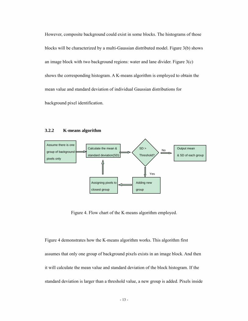
3.2.2 K-means algorithm

Figure 4. Flow chart of the K-means algorithm employed.

Figure 4 demonstrates how the K-means algorithm works. This algorithm first

assumes that only one group of background pixels exists in an image block. And then

it will calculate the mean value and standard deviation of the block histogram. If the

standard deviation is larger than a threshold value, a new group is added. Pixels inside

Assume there is one

group of background

pixels only

Calculate the mean &

standard deviation(SD)

SD >

Threshold?

Adding new

group

Output mean

& SD of each group

Yes

No

Assigning pixels to

closest group

- 14 -

the block will be assigned to the closest group, the mean value and standard deviation

of each group will be recalculated. The algorithm will output the mean value and

standard deviation of all background regions only when the standard deviation of each

group is smaller than a threshold value, or the number of groups is larger than two.

3.2.3 Foreground detection

Figure 5. Histogram of an image block with two background regions.

When the system goes into the detection phase, each image pixel will be examined

with respect to its own image block histogram. It will be first assigned to the closest

background region as follow: let there are two background regions exist in a block,

group A and group B as shown in Figure 5, with mean values Ma, Mb and standard

deviations SDa and SDb respectively. Let p be one of the pixels of the block.

- 15 -

If

absolute difference between p and Ma is smaller than that between p and Mb

then

p belongs to group A.

else

p belongs to group B.

Assume that p belongs to group A in this example. If the pixel value of p falls into the

region under the curve of A, p is a background pixel, otherwise, it belongs to

foreground. This process could be explained as follow:

If

absolute ( p - Ma ) < N x SDa i.e p falls into the region under the

curve of A

then

p is a background pixel

else

p is a foreground pixel

The value of N is determined empirically.

- 16 -

Any detected background pixel will be added into its own image block histogram,

which will be used to do the foreground detection for the next image frame.

3.2.4 Median filter

(a) (b)

(c)

Figure 6. (a) Original image; (b) image after background subtraction; (c) image after

median filtering.

- 17 -

Every input image with foreground objects will be processed by the background

subtraction module, and the foreground objects will be extracted and form an output

image, which is presented in Figure 6(b). This output image will be processed by a

median filter to remove some noise caused by background subtraction, and the result

is shown in Figure 6(c).

Figure 7. Calculating the median value of a pixel neighborhood. [7]

A spatial median filter is employed in the system to remove the speckle noise in

intermediate result. Each pixel in the image will be examined by the median filter in

turn; this filter looks at each pixel’s neighbors to find a representative value of its

surroundings. The median of neighboring pixel values will replace the current

examining pixel value. The median is determined as follow: start by sorting all

surrounding neighborhood pixel values as well as the pixel being examined, into

- 18 -

numerical order. And then the pixel being examined will be replaced with the middle

pixel value. An illustration is given in Figure 7, where a 3x3 square neighborhood is

used. The pixel at the center with pixel value 150 is being examined, and it is replaced

with the middle pixel value 124 after sorting all neighboring pixel values into

numerical order.

3.3 Analysis module

After the background subtraction process, some morphological operations will be

performed in order to obtain a better shape of the target objects. The first

morphological operation is dilation.

3.3.1 Dilation operation

Dilation is a basic operation in mathematical morphology. E is defined as an

Euclidean space, A is a binary image in E, and B is a structuring element. The dilation

of A by B is defined by [8]:

(1)

- 19 -

(a) Image after background (b) Image after dilation

subtraction.

Figure 8. Result of dilation operation.

The effect of the dilation operation is to enlarge the foreground regions, while holes

within those regions could be filled up. Besides, nearby disjoint foreground objects

could be connected. Figure 8 shows the result of this operation. Figure 8(a) is the

image before dilation. We can see that the swimmer’s body is separated into several

disjoint parts after the background subtraction, and some holes exist inside the body

region. Figure 8(b) is the result image of dilation operation. The holes inside the body

region are filled up and those disjoint parts are reconnected to form a complete human

body.

- 20 -

Figure 9. 8-connected neighborhood.

(a) Before dilation (b) After dilation

Figure 10. Illustration of dilation operation - white pixel: background; black pixel :

foreground.

An 8-connected neighborhood scheme is employed in the dilation operation. For a

pixel p shown in Figure 9, the eight pixels surrounding it are considered as its

8-connected neighbors. This 8-connected neighborhood scheme considers each pixel

in the image in turn. Assume p is a background pixel. If at least one of its 8-connected

p p p p

- 21 -

neighbors is a foreground pixel, it will be changed to the foreground pixel as well.

Figure 10 illustrates this process. In Figure 10(a), p is a background pixel, but one of

its 8-connected neighbors is a foreground pixel. So p will be changed to a foreground

pixel. This operation will examine every pixel in the image and finally the foreground

region will be expanded, as shown in Figure 10(b).

3.3.2 Erosion operation

Since the dilation operation will expand the size of foreground objects, an opposite

morphological operation, erosion, is applied on the result of dilation in order to shrink

the size of those foreground objects. Erosion is another basic operation in

mathematical morphology. Assume that E is an Euclidean space, A is a binary image

in E, and B is a structuring element. The erosion of A by B is defined by:

(2)

where Bz is the translation of B by the vector z.[9]

- 22 -

(a) Image after dilation (b) Image after erosion

Figure 11. Result of erosion operation.

Figure 11(a) shows an image after the dilation operation. The foreground objects are

expanded in this image. An erosion operation is applied on this image, which aims to

shrink the size of foreground objects. The result is shown in Figure 11(b), in which

the size of foreground objects is reduced, and the contours are improved.

(a) Before erosion (b) After erosion

Figure 12. Illustration of erosion operation - white pixel: background; black pixel :

foreground.

p p

- 23 -

Again, the 8-connected neighborhood is employed here. Every pixel in the image

will be considered by this 8-connected neighborhood scheme. As shown in Figure

12(a), if p is a foreground pixel and at least one of its 8-connected neighbors is a

background pixel, it will be changed to a background pixel. After all pixels are

examined, the foreground object will be shrunk as shown in Figure 12(b).

3.3.3 Boundary extraction

After the erosion operation, the contours of foreground objects are repaired. The next

step is to obtain the boundary of those foreground objects, which is critical

information for the subsequent steps in the analysis module. A boundary extraction

operation is employed to handle this task.

(a) Image before boundary extraction (b) Image after boundary extraction

Figure 13. Result of boundary extraction.

- 24 -

Boundary extraction aims to preserve the boundary pixels of foreground objects while

removing all other foreground pixels. Those boundary pixels represent the contours of

the foreground objects, which are valuable data for further analysis. With the interior

foreground pixels removed, the analysis can be performed more efficiently. Figure

13(a) shows an image before the boundary extraction. After the boundary extraction

operation, only the boundary pixels of foreground objects remained as shown in

Figure 13(b).

Figure 14. Illustration of boundary extraction operation.

The operation of boundary extraction could be explained as follow:

Step 1. Apply erosion operation on the original image.

Step 2. Subtract the eroded image by the original image.

Step 3. The pixels remained are the boundary pixels.

(a) Original image (b) Image after

erosion

(c) Image with

boundary pixels

only

- 25 -

The above process is illustrated in Figure 14, where Figure 14(b) is the eroded image

obtained from the original image of Figure 14(a). Figure 14(c) shows the image of

boundary pixels obtained by the subtraction process.

3.3.4 Removing the non-body objects

(a) Image with foreground and (b) Image after removing the

background objects background objects

Figure 15. Removal of non-body objects.

Figure 15(a) shows an image after the boundary extraction operation. Many small

connected regions remain after the background subtraction operation. These

connected regions, representing non-stationary background regions, will be

considered as non-body objects and removed by a non-body removal scheme. This

scheme works as follow:

- 26 -

Labeling all connected regions in the image as objects

For each of those objects

if

Its area is smaller than a threshold value

then

the object is removed.

The process of labeling the connected regions mentioned above employs a connected

component labeling algorithm. This algorithm uses a two-pass approach [10]:

On the first pass:

Step 1. Scan each pixel on the image.

Step 2. If the pixel is a foreground pixel.

1. Get its 8-connected neighboring pixels.

2. If there are no neighbors, assign a new label for the current

pixel and continue.

3. Otherwise, find the smallest label in the neighbors and assign it

to the current pixel.

4. Store the equivalence between neighboring labels.

- 27 -

On the second pass:

Step 1. Scan each pixel on the image.

Step 2. If the pixel is a foreground pixel.

1. Re-label the pixel with the smallest equivalent label.

The process discussed above is illustrated in Figure 16.

(a)

(b)

(c)

- 28 -

Figure 16. Connected component labeling: (a) Input image with foreground pixels of

1; (b) Result of first pass - check 8-connected neighbors for labeling and equivalent

labels are indicated; (c) Result of second pass - replacing all equivalent labels with the

smallest label.

3.3.5 Extracting extremal points

Figure 17. Process of extracting extremal points.

After the boundary image is obtained by the boundary extraction operation, some

extremal points on the human body have to be located. Those extremal points include

the legs and hands. However, before we could do that, the centroid of the human body

Centroid distance

Border position

distance

Border position Averaging

Filtering

(a)

(b)

(c) (d)

- 29 -

has to be determined first. Since position of the boundary pixels are already known,

the position of the centroid can be calculated as follow:

Let ( cx , cy ) be the position of the centroid, then

∑ == N

i ixN 1c1x (3)

∑ == N

i iyN

y1c

1 (4)

where N is the total number of boundary pixels, ( ix , iy ) is the position of a pixel on

the boundary.

After we get the centroid of the human body as shown in Figure 17(a), the distance

between each boundary pixel and the centroid, as shown in Figure 17(b), is calculated

as follow:

2)(2)(c

yi

yc

xi

xi

d −+−= (5)

The distance profile in Figure 17(b) is very fluctuating. An averaging filter is applied

to remove the noise, and the result is shown in Figure 17(c).

Those local maxima in Figure 17(c) are taken as the extremal points, and the image in

- 30 -

Figure 17(d) is constructed by connecting all those extremal points to the centroid.

The local maxima can be determined by finding the zero-crossings in the difference

function.

1−−= iii ddδ (6)

3.3.6 Locating interested points

(a) (b)

Figure 18. (a) Interested points located in the boundary image. (b) Interested points

overlaid on the original image.

Some interested points have to be located in the upper part of the human body. They

include the shoulders, elbows and hands. A skeleton can be constructed to represent

the upper part of the body by connecting those interested points, which is shown in

Figure 18(a). Figure 18(b) illustrates how accurate the locating mechanism with the

Centroid

Shoulders

Elbows

Hands

- 31 -

interested points overlaid on the original image.

Since the position of two hands and the centroid are already known from the previous

step, the locating mechanism only needs to locate the elbows and shoulders, which is

illustrated in below.

Figure 19. Locating elbow position.

Figure 19 illustrates how the elbows can be located. Since the positions of two hands

are known, by calculating the average value of those two positions, the point d can be

located. A line can be constructed by connecting point d to the centroid. This line is

broken into two parts with a predefined ratio, and then point e can be located. A

horizontal line L, which crosses point e, is formed. Start from point e and search along

d

e

L

- 32 -

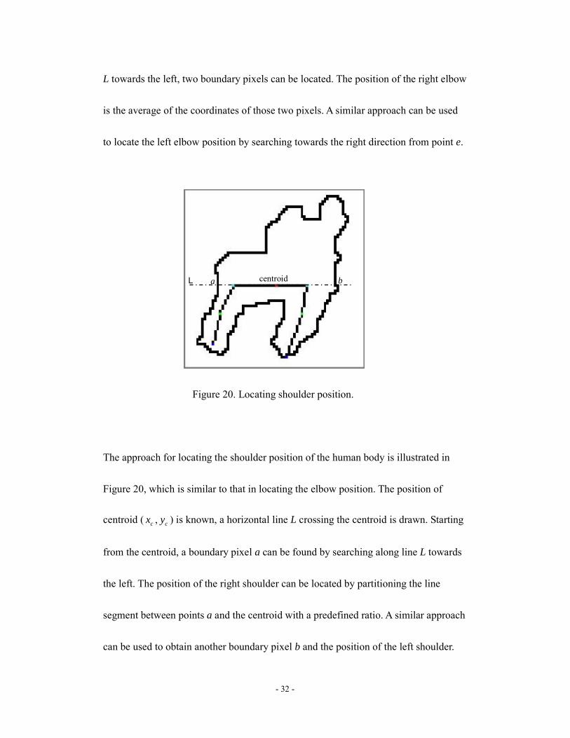
L towards the left, two boundary pixels can be located. The position of the right elbow

is the average of the coordinates of those two pixels. A similar approach can be used

to locate the left elbow position by searching towards the right direction from point e.

Figure 20. Locating shoulder position.

The approach for locating the shoulder position of the human body is illustrated in

Figure 20, which is similar to that in locating the elbow position. The position of

centroid ( cx , cy ) is known, a horizontal line L crossing the centroid is drawn. Starting

from the centroid, a boundary pixel a can be found by searching along line L towards

the left. The position of the right shoulder can be located by partitioning the line

segment between points a and the centroid with a predefined ratio. A similar approach

can be used to obtain another boundary pixel b and the position of the left shoulder.

L a b L a b centroid

- 33 -

3.4 Tracking module

Figure 21. Illustration of Kalman filter.

In the tracking module, we assume that the swimmer swims at a constant velocity. A

Kalman filter is employed for tracking the target object. The employed Kalman filter

can estimate the position of the swimmer recursively, where the position of the

swimmer is represent by the centroid of the body part. Figure 21 illustrates how this

filter works. Five major equations are used and they are separated into two models:

the prediction model and the correction model. The first equation in the prediction

model predicts the current position of the human body part by using the last estimated

Prediction Model Correction Model

Initial Value of

and

Predict the position

Predict the error covariance

Calculate the Kalman gain

Update estimate with measurement

Update the error covariance

- 34 -

value, where k

S − is the current predicted value for the position, 1−k

S is the last

estimated value, V is the constant velocity, T∆ is the time between two consecutive

video frames, Wk is the random noise variable. The second equation in the prediction

model predicts the error covariance ahead, where k

P − is the predicted error

covariance, 1−k

P is the last estimated error covariance, Q is the error covariance of

the random noise variable Wk. Both the predicted position value

kS − and

kP − will

be input into the correction model for correction. The first equation in the correction

model outputs the Kalman gain, where k

K is the Kalman gain, k

P − is the error

covariance of predict value, R is the error covariance of the measurement value. The

second equation in the correction model calculates the estimated value for the position

by using the predicted value of the positionk

S − , the measurement value of the position

kZ and the Kalman gaink

K . The third equation in the correction model updates the

error covariance. Both the estimated value of position kS and updated error

covariance kP will be input back into the prediction model for predicting the next

position value. Therefore, after inputting the initial estimates for 1−kS and 1−kP , the

Kalman filter can run recursively, the Kalman gain and other variables can be updated

automatically.

- 35 -

Chapter 4 Result

4.1 System Configuration

This final year project is developed on a notebook computer with the following

configuration:

CPU: Intel Core(TM) 2 Duo CPU P8600, 2.40GHz

Memory: 2 GB

Hard disk: 200 GB

Operation system: Windows Vista

The program of this project is implemented in C++ programming language with

Microsoft Visual Studio 2008 software kit. The libraries used in this project are listed

in below:

#include <stdlib.h>

#include <iostream>

#include <fstream>

#include <string>

#include <sstream>

#include <math.h>

The video data used for testing is in MPEG-2 format with a 720x576 resolution and

the frame rate is 25 fps.

- 36 -

4.2 Background Subtraction

Figure 22. Images in the first row are the original ones, images in the second

row are the corresponding results of background subtraction.

Figure 22 shows the results of background subtraction, where 30 image frames are

used for building up the initial background model. The major noises remained are the

pixels of the lane dividers on the water surface and those on the bottom of the

swimming pool. The lane divider on the water surface will float and wave due to the

move of water, which makes its position in different image frames be different, and

hence provides a great challenge to the background subtraction process, which

assumes that all background objects should be static. Besides, swimmer will make

ripples on the water surface when she/he is swimming. The constant color of the lane

divider on the bottom of the pool will be disturbed by the ripples. Both causes

- 37 -

contribute to non-stationary background pixels in the image which are difficult to be

remove by the background subtraction. However, the results shown in Figure 22 are

much better than the traditional frame difference approach. The figure below shows a

comparison of the two approaches.

Figure 23. Comparison between frame difference and region-based approach.

Since the frame difference approach simply perform the subtraction between an image

with foreground objects with a background image (template), a pixel is assigned as

foreground if its difference is larger than a threshold value. However, the variation of

the pixel value is very large. No matter using a low threshold (30) or a relatively high

threshold (100), there are still many background objects remained after the

background subtraction. The result of using a low threshold and high threshold is

shown in Figure 23(a) and (b) respectively. Figure 23(c) shows the result of using the

Input Image

Frame Difference

Region-based

(a) Low Threshold (b) High Threshold

(c)

- 38 -

region-based approach we proposed. The background objects remained in the image is

comparatively much less than that using the frame difference approach, and it

demonstrates that the performance of the region-based approach is much better than

the frame difference approach in doing background subtraction in the aquatic

environment. It is because the region-based approach constructs the background

model in blocks. When classifying a pixel as foreground or background, the pixel is

compared with the Gaussian distributed model of its own image block, not just

compared with the corresponding pixel values in previous frames only. Therefore, the

region-based approach is less sensitive to the variation of pixels value and hence

achieves a better performance.

- 39 -

4.3 Median Filter

(a)

(b) (c) (d)

Figure 24. Median filtering (a) image after background subtraction; (b), (c) and (d)

images after applying median filter on (a) with window size 3x3, 9x9 and 15x15

respectively.

The median filter can effectively remove the background objects still remained after

the background subtraction operation, and the results are shown in Figure 24. The

larger the window size used in the median filter operation, more background objects

could be removed. The result shown in Figure 24(d) uses the largest window size, so

the background objects remained are the least. However, a larger window size can

also affect the shape of the foreground region (human) more. Figure 24(b) uses the

smallest window size, so the shape of the human body is most similar to that in Figure

- 40 -

24(a). Therefore, by considering the effect on the shape of the human body and the

strength of the noise reduction, the window size of 9x9 is considered as the best for

median filtering and Figure 24(c) shows the result.

4.4 Morphological Operations

- 41 -

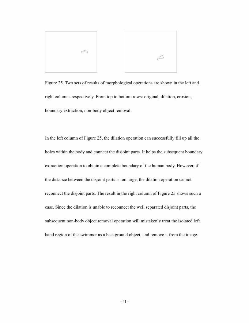
Figure 25. Two sets of results of morphological operations are shown in the left and

right columns respectively. From top to bottom rows: original, dilation, erosion,

boundary extraction, non-body object removal.

In the left column of Figure 25, the dilation operation can successfully fill up all the

holes within the body and connect the disjoint parts. It helps the subsequent boundary

extraction operation to obtain a complete boundary of the human body. However, if

the distance between the disjoint parts is too large, the dilation operation cannot

reconnect the disjoint parts. The result in the right column of Figure 25 shows such a

case. Since the dilation is unable to reconnect the well separated disjoint parts, the

subsequent non-body object removal operation will mistakenly treat the isolated left

hand region of the swimmer as a background object, and remove it from the image.

- 42 -

4.5 Locating Interested Points

Figure 26. (a) A skeleton is drawn on the boundary image with the located

interested points. (b) Interested points are overlaid on the original image.

Figure 26 shows the result of successfully locating the interested points. A skeleton is

constructed with those located interested points. This skeleton is valuable information

for other project such as human motion recognition, because by finding the angles

between those points, high-level interpretation could be done. Those interested points

are also highlighted and overlaid on the original image for performance evaluation. It

can be seen that the accuracy of the locating process is quite high in this case.

Figure 27. An unsuccessful case on locating interested points.

Centroid

Shoulders

Elbows

Hands

Centroid

Shoulders

Elbows

Hands

- 43 -

The performance of the locating process is heavily relied on the quality of the

boundary of human body obtained. If the human body obtained is incomplete, the

performance of the locating process will deteriorate. Figure 27 shows such a case.

Although the position of the centroid is acceptable, all other interested points are

located incorrectly.

4.6 Tracking Process

4.6.1 Result of Kalman Filter

Kalman F ilter Result

0

50

100

150

200

250

300

350

400

1 6 11 16 21 26 31 36 41 46 51 56 61 66 71 76 81

Frame Number

Position(Y-coordinate)

Measured

P redicted

Estimated

Kalman Filter Result

0

100

200

300

400

500

600

700

1 6 11 16 21 26 31 36 41 46 51 56 61 66 71 76 81

Frame Number

Position(X-coordinate)

Measured

Estimated

Predicted

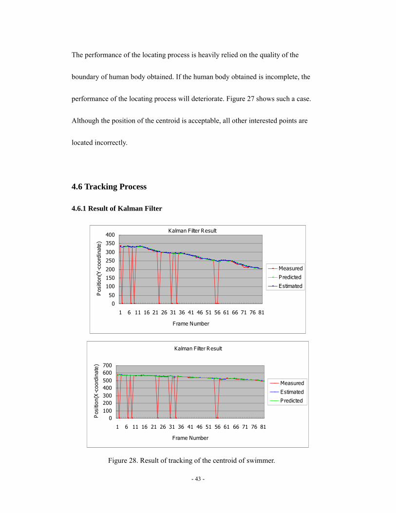
Figure 28. Result of tracking of the centroid of swimmer.

- 44 -

The Kalman filter has been tested on some video clips. Figure 28 shows the result of

tracking the centroid of a swimmer on one video clip. We can see that the measured

position, predicted position and estimated position are close to each other most of the

time. For the cases that there are large errors in the measured value, the estimated

value will be shifted towards the predicted value, and the tracking process can go on.

The reason why the measured value drops to zero in some frames is that in some

frames the swimmer is occluded by the splash. The background subtraction could not

extract the body region successfully, and therefore there is no measured data.

(a) (b) (c)

(d) (e) (f)

Figure 29. Applying Kalman filter on tracking interested points.

Centroid Shoulders

Elbows Hands

- 45 -

The Kalman filter is also applied on tracking the movement of those interested points,

which aims to assist the locating process. The results are shown on the Figure 29. The

accuracy of this tracking process is high for the gestures when the two hands are

stretched out. The performance will deteriorate when both hands are pulled back

underneath the body - a self-occlusion problem.

4.6.2 Object Tracking

Figure 30. From left to right, from top to bottom. A rectangle is drawn around

the body part of the swimmer.

- 46 -

Figure 30 shows the tracking of a swimmer on a video clip. A green rectangle is

drawn around the body part of the swimmer to illustrate the performance of the

tracking process. The rectangle is constructed by using the estimated positions of the

centroid as the center, and its size is determined by the body part obtained in the

background subtraction process. The tracking process focuses on the upper part of the

body, so the size of this bounding rectangle will change according to the stretch of the

two hands. We can see from Figure 30 that the tracking performance is good since the

rectangle can enclose the body part most of the time.

- 47 -

Chapter 5 Discussion

We proposed a region-based approach for the background modeling process, which

is less sensitive to the wide change of background pixels along the image sequence.

Therefore, the results in the background subtraction are quite acceptable. Some

interested points can be located on the upper part of the body, which will be valuable

information for motion recognition. Besides, the tracking module can also

successfully track the motion of the swimmer by employing the Kalman filter.

However, there are three major limitations exist in the system. The first one is that the

image frames used for building up the background model must come from a

stationary camera. It is because the region-based background subtraction heavily

relies on the information provided by previous frames. While light source variation

can be compensated by the adaptive updating of the background model, if the

background is spatially changing due to waving water, there is not reliable

information provided for this approach to determine whether a pixel belongs to

foreground or background. Nevertheless, this limitation exists in the traditional frame

difference approach too. In order to do background subtraction in a dynamic

environment, some researches used a skin model to identify the human body. A

- 48 -

specific color range will be used for the skin model. Any pixels fall into that range

will be considered as foreground, but this approach assumes that there are no

background objects with the same color range.

Another limitation exists in the analysis module, currently it is developed for

analyzing the breaststroke swimming style only. We focused on analyzing the

breaststroke since this swimming style has the following three advantages: 1) The

swimming speed of breaststroke style is relatively slow as compared with freestyle

and butterfly, which contributes a very small difference in two consecutive frames and

hence makes the human region easier to locate and analyze. 2) Breaststroke is a very

gentle swimming style with much less splash, which reduces the difficulty in

background subtraction. 3) In breaststroke swimming, the two hands will be stretched

out from the body most of the time, which makes them easier to be differentiated from

the trunk.

The last limitation exist in the system is that the Kalman filter employed in the

tracking module assumes that the swimmer swims at a constant speed, and the

prediction model in the filter is built up based on this assumption. However, even for

the same swimming style the swimming speed will not be constant all the time, which

- 49 -

contributes to a large error in the prediction. Hence the final estimated value is shifted

towards the measurement value. The tracking accuracy relies on the measurement

value, so if the accuracy of the measurement value is deteriorated due to a poor

background subtraction, the overall performance of the tracking module will be

downgraded. Future work can be done to solve this problem by increasing the

accuracy of the prediction model, which can be achieved by considering the

periodicity of the swimming motion.

- 50 -

Chapter 6 Conclusion

This final year project proposed a vision system for analyzing the swimmer’s motion.

We adopted a region-based approach in doing the background subtraction in order to

extract the human body from an image sequence of a swimming video. After

obtaining the human body part, some interested points including hands, elbows,

shoulders and the centroid will be located in the upper part of the body. These are

useful data for the subsequent project on human motion recognition. A tracking

process is also established on tracking the movement of the swimmer aiming to

acquire the trajectories of the body parts. Future work includes developing a tracking

process on tracing the movement of the interested points, which intends to increase

the accuracy on locating those interested points.

- 51 -

Reference

[1] J. Triesch; C. Von Der Malsburg: A gesture interface for human-robot-interaction.

Proceedings of the Third IEEE International Conference on Automatic Face and

Gesture Recognition. 14-16 April 1998, pp. 546 - 551

[2] http://www.detec.no

[3] H. L. Eng; K. A. Toh; W. Y. Yau; J. X. Wang:

DEWS: A Live Visual Surveillance System for Early Drowning Detection at Pool.

IEEE Transactions on Circuits and Systems for Video Technology, Vol. 18, No. 2, Feb.

2008, pp. 196-210

[4] H. L. Eng; J. W; S. W. Kam and W. Y. Yau: Robust Human Detection Within a

Highly Dynamic Aquatic Environment in Real Time. IEEE Transactions on Image

Processing, Vol. 15, No. 6, June 2006, pp. 1583-1600

[5] H. Fujiyoshi; A. J. Lipton: Real-time Human Motion Analysis by Image

Skeletonization. Proceedings of Fourth IEEE Workshop on Applications of Computer

- 52 -

Vision, WACV '98. 19-21 Oct. 1998, pp. 15 - 21

[6] K. L. Chan: Video-Based Gait Analysis By Silhouette Chamfer Distance and

Kalman Filter. International Journal of Image and Graphics, Vol. 8, No. 3, July 2008,

pp. 383-418

[7] http://homepages.inf.ed.ac.uk/rbf/HIPR2/median.htm

[8] http://en.wikipedia.org/wiki/Dilation_(morphology)

[9] http://en.wikipedia.org/wiki/Erosion_(morphology)

[10] http://en.wikipedia.org/wiki/Connected_Component_Labeling