Helsinki University of Technology Communications Laboratory Technical Report T54

Teknillinen korkeakoulu Tietoliikennelaboratorio Raportti T54

Espoo 2006

STUDIES ON THE PERFORMANCE OF SOME ARQ SCHEMES

Markku Liinaharja

Dissertation for the degree of Doctor of Science in Technology to be presented with due permission for publicexamination and debate in Auditorium S4 at Helsinki University of Technology (Espoo, Finland) on the 31st

of March, 2006, at 12 o’clock noon.

Helsinki University of TechnologyDepartment of Electrical and Communications EngineeringCommunications Laboratory

Teknillinen korkeakouluSahko- ja tietoliikennetekniikan osastoTietoliikennelaboratorio

Distributor:Helsinki University of TechnologyCommunications LaboratoryP.O. Box 3000FI-02015 TKKTel. +358-9-451 2366Fax +358-9-451 2345

c©Markku Liinaharja

ISBN 951-22-8114-7 (printed)ISBN 951-22-8115-5 (electronic)ISSN 0356-5087

Otamedia OyEspoo 2006

Abstract

This thesis consists of a summary part and seven published articles. All the articles are aboutperformance analysis of ARQ schemes.

Two of the publications study the performance of an ARQ scheme with packet combining, calledthe EARQ (extended ARQ) scheme. In the packet combining algorithm, the bitwise modulo-2sum of two erroneous copies of a packet is computed to locate the errors. The packet combiningalgorithm involves a straightforward search procedure, the computational complexity of whicheasily becomes prohibitive. As a solution to this, a modifiedscheme is proposed, where thesearch procedure is attempted only when there are at mostNmax 1s at the output of the modulo-2adder. In one article, time diversity was utilized, whereasspace diversity reception was consi-dered in the other work.

The remaining five publications study the throughput performance of adaptive selective-repeatand go-back-N ARQ schemes, where the switching between the transmission modes is donebased on the simple algorithm proposed by Y.-D. Yao in 1995. In this method,α contiguousNACKs or β contiguous ACKs indicate changes from ‘good’ to ‘bad’ or from ‘bad’ to ‘good’channel conditions, respectively. The numbersα andβ are the two design parameters of theadaptive scheme. The time-varying forward channel is modelled by two-state Markov chains,known as Gilbert-Elliott channel models. The states are characterized by bit error rates, packeterror rates or fading parameters. The performance of the adaptive ARQ scheme is measuredby its average throughput over all states of the system model, which is a Markov chain. Auseful upper bound for the achievable average throughput isprovided by the performance ofan (assumed) ideal adaptive scheme which is always in the ‘correct’ transmission mode. Theoptimization ofα andβ is done based on minimizing the mean-square distance between theactual and the ideal performance curves. Methods of optimizing the packet size(s) used in theadaptive selective-repeat scheme are also proposed.

Keywords: adaptive protocol, automatic repeat request, diversity combining, error control, Mar-kov model, packet combining

iii

Tiivistelma

Tama vaitoskirja sisaltaa johdanto-osan ja seitseman julkaistua artikkelia. Kaikki artikkelit tut-kivat ARQ-protokollien suorituskyvyn analysointia.

Julkaisuista kaksi kasittelee EARQ:ksi nimettya laajennettua ARQ-protokollaa, missa pyritaanloytamaan vastaanotetuissa paketeissa olevia virheita yhdistamalla saman datapaketin kaksi vir-heellisina vastaanotettua kopiota keskenaan. Yhdist¨aminen tapahtuu laskemalla bittivektorit yh-teen modulo 2. Algoritmiin kuuluu suoraviivainen oikean koodisanan hakuprosessi, jonka las-kennallinen kompleksisuus kasvaa nopeasti kohtuuttoman suureksi. Taman ongelman ratkai-suksi ehdotetaan muunnettua algoritmia, missa hakurutiini kaynnistetaan vain, jos modulo-2-summaimen ulostulossa on korkeintaanNmax ykkosta. Artikkeleista toisessa kasitellaan aika-ja toisessa puolestaan paikkadiversiteetin hyodyntamista.

Loput viisi julkaisua tutkivat adaptiivisten ARQ-protokollien suorituskykya. Tehokkuutta mi-tataan lapaisylla (throughput), ja kasiteltavanaovat seka valikoivaa toistoa hyodyntavat SR-protokollat (selective repeat) etta liukuvaa lahetysikkunaa kayttavat go-back-N -protokollat.Tarkasteltavissa adaptiivisissa protokollissa lahettimella on kaksi tilaa, joiden valilla siirrytaanY.-D. Yaon vuonna 1995 esitteleman algoritmin mukaisesti: α perakkaista negatiivista kuit-tausta (eli uudelleenlahetyspyyntoa) merkitsee, ett¨a kanavan tila on todennakoisesti muuttu-nut ‘hyvasta’ ‘huonoksi’;β perakkaista positiivista kuittausta puolestaan tulkitaan merkiksipainvastaisesta muutoksesta. Luvutα ja β ovat talla periaatteella toimivan adaptiivisen proto-kollan kaksi suunnitteluparametria. Aikavaihtelevia lahetyskanavia mallinnetaan kaksitilaisillaMarkovin ketjuilla, joita nimitetaan Gilbert-Elliott -kanavamalleiksi. Kanavan tila maaritellaanjoko bittivirhetodennakoisyyden, pakettivirhetodennakoisyyden tai haipymisparametrien avul-la. Koko systeemin tilamalli osoittautuu Markovin ketjuksi, ja adaptiivisen protokollan suori-tuskykya mitataan laskemalla sen keskimaarainen lapaisy yli kaikkien tilojen. Saavutettavissaolevalle keskimaaraiselle lapaisylle saadaan ylaraja laskemalla lapaisy hypoteettiselle ideaali-selle adaptiiviselle protokollalle. Optimaalinen(α, β)-pari on se, jota vastaava lapaisykayra onlahimpana ideaalista kayraa pienimman neliovirheen mielessa. Lisaksi julkaisuissa on tutkittukaytettavan pakettikoon optimointia adaptiivisille SR-protokollille.

Avainsanat: adaptiivinen protokolla, ARQ, diversiteettiyhdistely, Markov-malli, virheentark-kailu

iv

Preface

The research work for this thesis was done at the Communications Laboratory of HelsinkiUniversity of Technology during 1997–2005. In the early years, the work was funded bythe Academy of Finland, the National Technology Agency of Finland (TEKES), Nokia Re-search Center (NRC) and Ericsson Ltd. Since the autumn of 2002, my work has been financedby the Graduate School in Electronics, Telecommunicationsand Automation (GETA), and theAcademy of Finland under grant 100500. The additional funding from Jenny and Antti WihuriFoundation is also gratefully acknowledged.

I am grateful to Professor PatricOstergard, the supervisor of this thesis, for helping me togetthis work finished and for many helpful comments.

I thank Dr. Shyam Chakraborty for directing the research work and for several years of inter-esting collaboration.

I appreciate very much the thorough job done by the two pre-examiners of my thesis, Prof. T.Aaron Gulliver and Dr. Ulrich Tamm. I received several useful comments, which improved thequality of the manuscript.

I also want to thank the entire staff of the Communications Laboratory for making it such apleasant working environment, as well as all the other people who have one way or anotherhelped me.

Espoo, 9th March, 2006

Markku Liinaharja

v

Contents

Preface v

List of Abbreviations ix

List of Symbols x

List of Publications xi

1 Introduction 1

1.1 Motivation . . . . . . . . . . . . . . . . . . . . . . . . . . . . . . . . . . . . . 1

1.2 Background: ARQ and FEC . . . . . . . . . . . . . . . . . . . . . . . . . . . 1

1.3 Scope and Structure of the Thesis . . . . . . . . . . . . . . . . . . . .. . . . 2

2 Basic Concepts 5

2.1 Channel Models . . . . . . . . . . . . . . . . . . . . . . . . . . . . . . . . . . 5

2.1.1 Discrete-Time Models . . . . . . . . . . . . . . . . . . . . . . . . . . 5

2.1.2 Threshold Model for Fading Channels . . . . . . . . . . . . . . .. . . 7

2.2 Performance Measures . . . . . . . . . . . . . . . . . . . . . . . . . . . . .. 8

2.2.1 Throughput Efficiency . . . . . . . . . . . . . . . . . . . . . . . . . . 8

2.2.2 Other Performance Measures . . . . . . . . . . . . . . . . . . . . . .. 8

2.3 Throughput Performance of Basic ARQ Schemes . . . . . . . . . .. . . . . . 9

vii

2.4 Improving Basic ARQ Schemes . . . . . . . . . . . . . . . . . . . . . . . .. 11

2.4.1 Selection of the Packet Size . . . . . . . . . . . . . . . . . . . . . .. 11

2.4.2 Use of Multicopy Transmissions . . . . . . . . . . . . . . . . . . .. . 12

2.5 Hybrid ARQ and Packet Combining . . . . . . . . . . . . . . . . . . . . .. . 14

2.5.1 HARQ-I Schemes . . . . . . . . . . . . . . . . . . . . . . . . . . . . 14

2.5.2 HARQ-II Schemes . . . . . . . . . . . . . . . . . . . . . . . . . . . . 15

2.5.3 Diversity Combining . . . . . . . . . . . . . . . . . . . . . . . . . . . 16

2.6 Adaptive ARQ . . . . . . . . . . . . . . . . . . . . . . . . . . . . . . . . . . 16

3 Adaptive ARQ Schemes Based on Yao’s Algorithm 19

3.1 Yao’s Channel Sensing Algorithm . . . . . . . . . . . . . . . . . . . .. . . . 19

3.2 Related Work . . . . . . . . . . . . . . . . . . . . . . . . . . . . . . . . . . . 19

3.3 System Model and Throughput Analysis . . . . . . . . . . . . . . . .. . . . . 20

3.4 Parameter Optimization . . . . . . . . . . . . . . . . . . . . . . . . . . .. . . 27

3.4.1 Optimization of the Packet Size . . . . . . . . . . . . . . . . . . .. . 27

3.4.2 Optimization ofα andβ . . . . . . . . . . . . . . . . . . . . . . . . . 28

3.5 Summary of Optimization Results . . . . . . . . . . . . . . . . . . . .. . . . 28

4 ARQ with Diversity Combining 31

4.1 The EARQ Scheme with Time Diversity . . . . . . . . . . . . . . . . . .. . . 31

4.2 Approximate Throughput Analysis . . . . . . . . . . . . . . . . . . .. . . . . 32

4.3 The EARQ Scheme with Spatial Diversity . . . . . . . . . . . . . . .. . . . . 34

5 Summary of Publications 39

6 Conclusions 43

viii

List of Abbreviations

ACK positive acknowledgementARQ automatic-repeat-requestAWGN additive white gaussian noiseBER bit error rateCRC cyclic redundancy checkEARQ extended ARQGBN go-back-NG-E Gilbert-ElliottHARQ hybrid ARQHARQ-I type I HARQHARQ-II type II HARQHMM hidden Markov modelISR ideal selective-repeatNACK negative acknowledgementOBI observation intervalPER packet error rateRCC rate compatible convolutionalSW stop-and-waitSR selective-repeatXOR exclusive-OR

ix

List of Symbols

L transmission mode for low error ratesH transmission mode for high error ratesα OBI length in modeLβ OBI length in modeHη throughputT packet throughputN transmitter buffer length in GBN protocoln packet size in bitsǫ bit error rateh number of overhead bits per packetPc probability of error-free transmissionnopt optimal packet sizeǫco crossover BERPf probability of acknowledgement errorPe packet error ratem number of copies used in multicopy GBN schemePco crossover PERG good state of forward channelB bad state of forward channelγ transition probability fromG to Bδ transition probability fromB to Gg good state of return channelb bad state of return channelλ transition probability fromg to bµ transition probability fromb to gηave average throughput of adaptive SR schemeηideal average throughput of ideal adaptive SR schemeπG steady-state probability of stateGπB steady-state probability of stateBǫ1 BER in stateGǫ2 BER in stateBPf,ave average probability of acknowledgement errorTave average packet throughput of adaptive GBN schemeTideal average packet throughput of ideal adaptive GBN schemePe,1 PER in stateGPe,2 PER in stateB

x

List of Publications

[P1] S.S. Chakraborty, E. Yli-Juuti, and M. Liinaharja. An ARQ scheme with packet combin-ing. IEEE Communications Letters,2:200–202, July 1998.

[P2] S.S. Chakraborty and M. Liinaharja. Analysis of adaptive SR ARQ scheme in time-varyingchannels.Electronics Letters,36:2036–2037, November 2000.

[P3] S.S. Chakraborty and M. Liinaharja. Performance analysisof an adaptive SR ARQ schemefor time-varying Rayleigh fading channels. InProceedings of ICC 2001,pages 2478–2482, June2001.

[P4] M. Liinaharja and S.S. Chakraborty. Analysis and optimization of an adaptive selective-repeat scheme for time-varying channels with feedback errors. AEU International Journal ofElectronics and Communications,56:177–186, March 2002.

[P5] S.S. Chakraborty, M. Liinaharja, and P. Lindroos. Analysis of an adaptive selective-rejectscheme in time-varying channel with non-negligible round-trip delay and erroneous feedback.Wireless Personal Communications,26:347–363, September 2003.

[P6] S.S. Chakraborty, M. Liinaharja, and P. Lindroos. Analysis of adaptive GBN schemes ina Gilbert-Elliott channel and optimization of system parameters.Computer Networks,48:683–695, July 2005.

[P7] S.S. Chakraborty, M. Liinaharja, and K. Ruttik. Diversityand packet combining in Rayleighfading channels.IEE Proceedings - Communications,152:353–356, June 2005.

For all the publications in this thesis, the work of the research group has been led by Dr.Chakraborty in the sense that he has outlined the topic and scope of each article. The author ofthis thesis has been responsible for most of the mathematical analysis and computing in thesepublications. The contributions of the author(s) are described in more detail below.

In publication [P1], the author of this thesis derived Equation (4), had an important part inwriting Sections II–IV together with the other authors, andalso wrote and ran the computerprograms both for simulation of the scheme and for the numerical computation of the approxi-mate throughput. The idea of the ARQ scheme that was studied came from the first author, whoalso wrote most of the text.

xi

In publication [P2], the author of this thesis wrote the second and the third section, and did allthe analysis and numerical computations. The observation that neither Yao nor Annamalai &Bhargava in their papers cited here had used a time-varying channel model was made by theauthor of this thesis. The formulation of the Markov model ofthe system and the definition ofthe ideal performance curve as an upper bound were also due tothe author of this thesis. Thesefindings played an important part also in [P3]–[P6]. The firstauthor wrote the introduction, andthe ideas of using half-size packets and acknowledging themin pairs are also due to him.

Publications [P3] and [P4] were written and the contents were produced almost completelyby the author of this thesis. In [P4], this author’s contributions include the formulation of theoptimization problem of the parametersα andβ in Yao’s algorithm for an adaptive ARQ schemeoperating on a two-state Markov channel (a similar approachwas used also in [P5] and [P6])and, in particular, a new method for the optimization of the packet lengths used by the adaptiveSR scheme (this method was used also in [P5]). Dr. Chakraborty contributed Fig. 2 in [P3], andsome improving comments in both of these publications.

In publications [P5] and [P6], the introductions and also most of the other parts of the text werewritten by the first author. Section 3.3 in [P6] was written completely by the author of thisthesis. The Markov models of the systems were constructed bythe author of this thesis andMr. Lindroos. Mr. Lindroos contributed the idea of how to make the number of states in thesystem model independent of the round-trip delay; all the rest of the performance analysis ofthe adaptive schemes and all the numerical computations were done by the author of this thesisalone.

In publication [P7], the author of this thesis assisted in writing the literature survey in the intro-duction, did the brief analysis in Section 3, plus wrote and ran the simulation programs. Thepaper was mostly written by the first author. All the simulation programs were built on top ofthe Matlab implementation of the Jakes channel model provided by Mr. Ruttik, who also wroteSection 4.1.

xii

Chapter 1

Introduction

1.1 Motivation

During the past couple of decades, digital communication has become ubiquitous. The simplestdigital communication system, a communicationlink, is shown in its most abstracted form inFigure 1.1. The task ofthe transmitteris to render the message suitable for transmission overthe channel.The channel is the physical medium that is used to convey the information fromthe transmitter to thereceiver. In [30, p. 15], communication channels are divided into twobasic groups: channels based onguided propagation(telephone channels, coaxial cables andoptical fibres), and channels based onfree propagation(wireless broadcast channels, mobileradio channels and satellite channels). The receiver reconstructs the message from the receivedsignal.

Channel ReceiverTransmitter

Figure 1.1: Digital communication link

The communication channels exhibit many kinds of non-idealbehaviour, such as additive noise,fading caused by multipath propagation, and intersymbol interference. As a result from thesephenomena, the received signal is often so badly distorted that the message cannot be recon-structed unless some kind oferror control is used.

1.2 Background: ARQ and FEC

There are two basic approaches to error control in digital communications:forward error cor-rection (FEC)andautomatic repeat request (ARQ)[44, 77].

1

In the FEC systems, parity-check bits are added to each transmitted message block to forma codeword based on the error-correcting code that is being used. The receiver attempts tolocate and correct the errors that it has detected in a received word. After the error-correctionprocedure, the decoded data block is delivered to the end user. A decoding erroroccurs if theoutput of the decoder is a different codeword than the one that was originally transmitted. TheFEC systems are designed for use in simplex channels, where information flows in only onedirection.

In an ARQ scheme, a high-rate error-detecting code is used together with some retransmissionprotocol. If the receiver detects errors in the received word,it generates a retransmission request,or a negative acknowledgement (NACK). If no errors are detected in the received word, thereceiver sends a positive acknowledgements, called an ACK,to the transmitter. The most widelyused error-detecting codes are the cyclic redundancy check(CRC) codes because of the ease ofimplementation. Unlike the FEC systems, the ARQ schemes require the presence of afeedbackchannel.

Thestop-and-wait (SW) schemeis the simplest of all ARQ schemes. In this scheme, the trans-mitter sends a codeword to the receiver and waits for an acknowledgement. If an ACK comes,the transmitter sends the next codeword in the queue; in caseof a NACK, the same codewordis retransmitted, and this process continues until the codeword is accepted. If the system hasa significant round-trip delay, the SW scheme becomes quickly very inefficient because of theidle time that the transmitter spends waiting for acknowledgements.

In thego-back-N (GBN)scheme, the transmitter sends codewords continuously and stores themto wait for acknowledgements; buffer space forN packets is needed at the transmitter. Theacknowledgement for a codeword arrives after a round-trip delay, during whichN − 1 othercodewords are transmitted. When a NACK is received for codeword i, the transmitter stopstransmitting new codewords, goes back to codewordi and retransmits it and theN − 1 fol-lowing codewords. The receiver discards the erroneously received codewordi and allN − 1subsequently received words, regardless if they are error-free or not.

Another continuous ARQ strategy,selective-repeat (SR)ARQ, is much more efficient thanGBN, since only negatively acknowledged codewords are retransmitted. After resending a neg-atively acknowledged codeword, the transmitter continuestransmitting new codewords in thetransmitter buffer. Whereas the GBN scheme automatically preserves the original order of thecodewords, the receiver in the SR scheme must have some buffer space to store the correctlyreceived codewords that can not yet be released.

If some error-correcting capability is added to an ARQ scheme, we have ahybrid ARQ (HARQ)scheme. HARQ schemes, which are thus combinations of ARQ andFEC, are discussed inSection 2.5.

1.3 Scope and Structure of the Thesis

This thesis consists of mainly theoretical studies on the performance of some ARQ schemes.Two kinds of schemes have been studied: (i) ARQ schemes with diversity combining in [P1]

2

and [P7], (ii) adaptive ARQ schemes in [P2]–[P6].

An ARQ scheme with packet combining (using time diversity) is studied in a random-errorchannel environment in [P1]. Approximate performance analysis is presented and the resultsare compared to simulations. The packet combining algorithm, based on computing the bit-wise modulo-2 sum of two erroneous copies of a packet was originally proposed by Sindhuin [67]. In [P7], the same scheme, referred to as the EARQ scheme (for ‘extended ARQ’) isused in a wireless communication system where there are two antennas at the receiver. That is,spatial diversity is utilized. The performances of the EARQscheme and three other schemesare compared in fading channels by simulations. A sum-of-sinusoids model, derived from thatproposed by Jakes in [32], is used to represent Rayleigh fading channels. The sinusoids haverandom frequency inside the Doppler spectrum, and random phase.

In [79], Yao proposes an adaptive GBN scheme with two transmission modes, denoted byL andH and meant for ‘good’ and ‘bad’ channel conditions, respectively. What is significant for thisthesis is that he suggests a simple algorithm for detecting channel state changes, which is basedon observing the acknowledgments and is defined by two integer-valued parameters:α andβ:if α contiguous NACKs are received by the transmitter when it is in modeL, it is concludedthat the channel conditions are deteriorating and the transmitter switches to modeH; if β ACKsare received contiguously while the transmitter is in modeH, modeL is resumed. In [3, 4]and a few other articles, Annamalai and Bhargava study adaptive GBN and SR schemes basedon Yao’s channel sensing algorithm; they also attempt to optimize the design parametersα andβ. However, no time-varying channel model where the channel state actually changes has beenspecified in these articles, and the same is true for Yao’s original paper. This is the startingpoint for the publications [P2]–[P6] of this thesis. In all these papers, the performance of theadaptive SR or GBN scheme using Yao’s algorithm is evaluatedin two-state Markovian channelenvironments under varying assumptions about the return channel and the round-trip delay.

The summary of the thesis is organized as follows. Chapter 2 reviews some basic concepts,including some channel models, performance measures of ARQschemes and hybrid ARQ.Chapter 3 is a survey of the contents of publications [P2]–[P6], while Chapter 4 covers publi-cations [P1] and [P7]. The summaries of all seven publications are provided in Chapter 5, andfinally some concluding remarks are made in Chapter 6.

3

4

Chapter 2

Basic Concepts

2.1 Channel Models

In order to evaluate the performance of error control systems, we must model the circumstanceswhere they operate. Here we take a somewhat limited perspective on modeling communicationchannels, and by achannel modelwe mean a mathematical model for the noise process or theerror process associated with the communication channel.

2.1.1 Discrete-Time Models

Most of the channel models considered in this work arediscrete-timemodels, which are charac-terized by the values of bit error rate (BER) or packet error rate (PER). Depending on whetherthe time unit of the model is the transmission time of one bit or one packet, these models can bedivided intobit-levelandpacket-levelmodels.

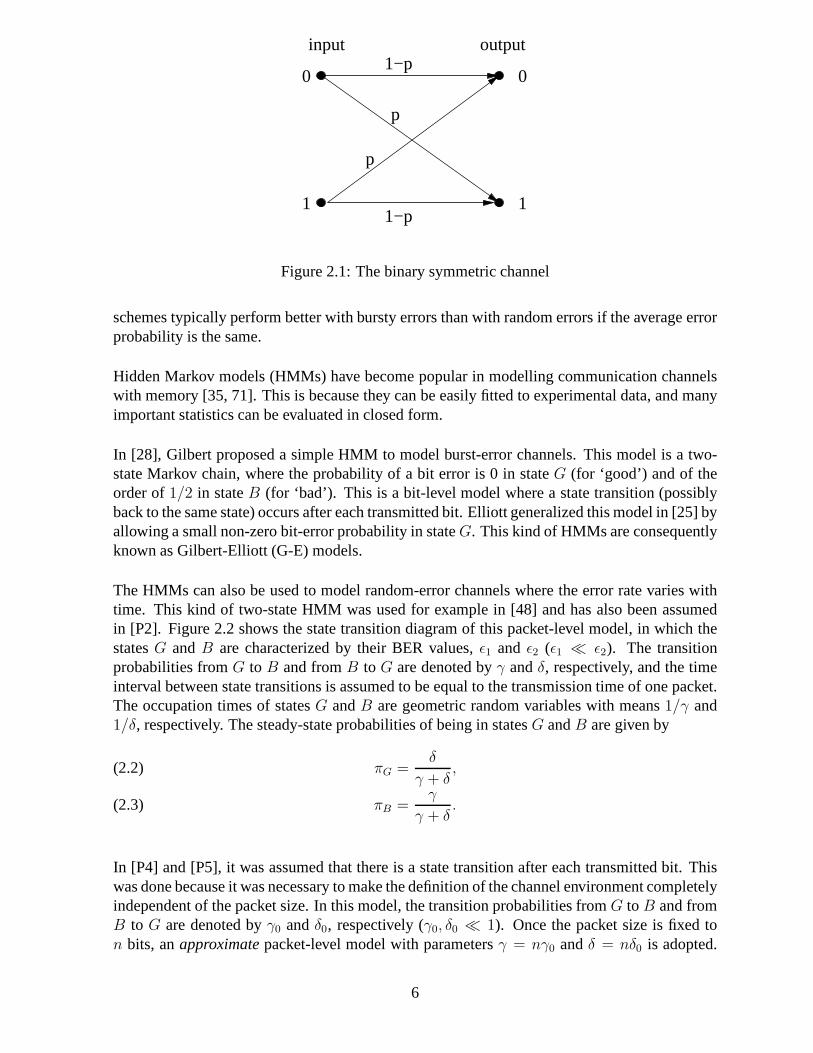
The simplest discrete-time model is the memoryless binary symmetric channel (BSC) [27, 59],which is also often referred to as therandom-errorchannel. In a BSC, a bit is received in errorwith a certain probability (the BER), independently of all the other bits. As a result, the numberof bit errors in a receivedn-bit packet is binomially distributed; if the BER is equal toǫ, thePER is given by

(2.1) Pe(n, ǫ) = 1 − (1 − ǫ)n.

A schematic picture of the BSC where the BER is equal top is shown in Figure 2.1.

In many practical channels, especially in the presence of fading, the bit errors are not statisticallyindependent, but occur in bursts. They are called channels with memory,orburst-errorchannels.If FEC is used and the error-correcting code is designed to correct random errors, the channelerrors can be made to look more random by using aninterleaverafter encoding the data blockand ade-interleaverbefore decoding the received word [59, 68]. On the other hand, ARQ

5

1−p

p

p

1−p

1

0

1

0

outputinput

Figure 2.1: The binary symmetric channel

schemes typically perform better with bursty errors than with random errors if the average errorprobability is the same.

Hidden Markov models (HMMs) have become popular in modelling communication channelswith memory [35, 71]. This is because they can be easily fittedto experimental data, and manyimportant statistics can be evaluated in closed form.

In [28], Gilbert proposed a simple HMM to model burst-error channels. This model is a two-state Markov chain, where the probability of a bit error is 0 in stateG (for ‘good’) and of theorder of1/2 in stateB (for ‘bad’). This is a bit-level model where a state transition (possiblyback to the same state) occurs after each transmitted bit. Elliott generalized this model in [25] byallowing a small non-zero bit-error probability in stateG. This kind of HMMs are consequentlyknown as Gilbert-Elliott (G-E) models.

The HMMs can also be used to model random-error channels where the error rate varies withtime. This kind of two-state HMM was used for example in [48] and has also been assumedin [P2]. Figure 2.2 shows the state transition diagram of this packet-level model, in which thestatesG andB are characterized by their BER values,ǫ1 and ǫ2 (ǫ1 ≪ ǫ2). The transitionprobabilities fromG to B and fromB to G are denoted byγ andδ, respectively, and the timeinterval between state transitions is assumed to be equal tothe transmission time of one packet.The occupation times of statesG andB are geometric random variables with means1/γ and1/δ, respectively. The steady-state probabilities of being instatesG andB are given by

πG =δ

γ + δ,(2.2)

πB =γ

γ + δ.(2.3)

In [P4] and [P5], it was assumed that there is a state transition after each transmitted bit. Thiswas done because it was necessary to make the definition of thechannel environment completelyindependent of the packet size. In this model, the transition probabilities fromG to B and fromB to G are denoted byγ0 andδ0, respectively (γ0, δ0 ≪ 1). Once the packet size is fixed ton bits, anapproximatepacket-level model with parametersγ = nγ0 andδ = nδ0 is adopted.

6

G B

γ

1−γ

δ

1−δ

Figure 2.2: The packet-level Gilbert-Elliott channel model

This approach makes it possible to compare the system performance with different packet sizesunder approximately similar channel conditions.

A packet-level G-E model was used also in [P6] with the difference that the statesG andBwhere defined by their PER values,Pe,1 andPe,2.

Unreliable return channels have also been considered in thepublications of this thesis. It hasbeen assumed that an acknowledgement, ACK or NACK, can be erased, but an ACK cannotbecome a NACK or vice versa. A similar assumption has been made e.g. in [11, 83]. In [P5]acknowledgements were erased randomly with probabilityPf , whereas in [P4] and [P6] a G-Emodel was assumed also for the feedback channel. In this G-E model, which is assumed to beindependent of the forward channel, all the acknowledgements are received successfully in the‘good’ state, which is denoted byg, but the probability of erasure isPf in the ‘bad’ state, whichis denoted byb.

2.1.2 Threshold Model for Fading Channels

If we use a somewhat simplified description, the average behaviour of a Rayleigh fading channelcan be described by two parameters:ρ andfD. Here,ρ is the ratio between the receiver thresholdpower and the average received signal power, i.e. a smaller value ofρ means that the channel isbetter on the average. The threshold power level is selectedso that if the instantaneous receivedsignal power is below the threshold value, it can be considered that there is a ‘fade’ going on.The other parameter,fD, is the maximum Doppler shift, which is equal tov/λ [32], wherev isthe velocity of the mobile terminal andλ is the carrier wavelength.

By using the level-crossing statistics presented in [32] and making some further simplifyingassumptions, DaSilva et al. derived in [21] a simple closed-form expression for the PER in afading channel described by the threshold model

(2.4) Pe(ρ, fD, n) = 1 − exp

[

−(

ρ +nfD

√2πρ

R

)]

,

wheren is the packet size in bits andR is the channel transmission rate in bits/s. The followingassumptions were made:

• The channel is in one of the two possible conditions at any time: the received signal poweris either above (‘non-fade interval’) or below (‘fade interval’) the threshold level.

7

• A packet is received correctly if and only if the whole packetwas contained in a non-fadeinterval.

• The length of the non-fade interval is exponentially distributed.

This PER expression was used by Annamalai and Bhargava in [4], and in [P3] a two-statepacket-level HMM was used, where the statesG andB were defined by the parameter combi-nations(ρ1, fD,1) and(ρ2, fD,2), respectively.

2.2 Performance Measures

2.2.1 Throughput Efficiency

The most important performance measure for the ARQ schemes is the throughput efficiency,or simply thethroughputη. The throughput is defined as the ratio of the average number ofinformation bits successfully accepted by the receiver perunit time to the total number of bitsthat could be transmitted per unit time [44]. It can be noted that the throughput of an FECscheme is a constant irrespective of the channel conditions, and it is equal to the rate of theerror-correcting code.

A related performance measure, which we will call thepacket throughputand denote byT , isdefined as the average number ofpacketsaccepted successfully per one transmission. It is theinverse number of the average number of transmission attempts needed until a packet is receivedsuccessfully. The difference betweenη andT is that in computingη, only the information bitsare considered ‘useful’, and henceη represents the ‘real’ transmission efficiency. The quantitiesη andT relate to each other as follows:

(2.5) η =k

n· T =

(k/n)

E[X],

wherek/n is the rate of the error-detecting code used by the ARQ scheme, andX is the randomvariable that represents the number of transmission attempts needed until a packet is receivedsuccessfully. Naturally, the distribution ofX depends on the channel (also the return channel)error statistics.

2.2.2 Other Performance Measures

Besides throughput, many other performance measures of ARQschemes have been proposedand studied. Most of these are related to the delay in delivering the packets.

As it was pointed out in [37], the total delay of a link layer packet consists of thetransportdelayand theresequencing delay.Of these two, the transport delay is further divided into the

8

queueing delayand thetransmission delay.In two early studies [40, 70], the authors derived thegenerating functions of the transport delay and the transmitter queue length for the basic ARQschemes when packet errors occur randomly and new packets arrive at the transmitter accordingto a Poisson process, and in [69] these studies were extendedto channels with memory. Themean queue length and mean transport delay for the SR scheme with arbitrary new packetarrival process and random errors were obtained in [2]. In [62], the authors derived the exactdistribution of thedelivery delay,which is the sum of transmission delay and resequencingdelay, for the SR scheme, when a two-state Markovian channelmodel was assumed. Randomerrors in both forward and return channels were assumed whenthe mean transmission delaywas calculated for the basic ARQ schemes in [46] using signalflow graphs, and the authorsgeneralized the analysis to Markovian channels in [47]. In arecent article [49], Luo et al.calculated the first and second order statistics for the delivery delay of a higher layer packetconsisting of a fixed number of link layer blocks, when the SR scheme was used in a randomerror channel environment. A delay related performance measure, namely the probability thata packet is not delivered withinD time slots of its arrival at the transmitter, has been studied in[63, 82].

In the recent years, communications between light portabledevices with finite battery resourceshave become increasingly important. Therefore,energy efficiencyis also an important perfor-mance measure of an error control strategy and has been discussed, e.g., in [18, 81].

2.3 Throughput Performance of Basic ARQ Schemes

The throughput of the SW scheme is given by [44]

(2.6) ηSW =Pc · (k/n)

1 + DR/n,

wherePc is the probability of a successful transmission,D is theround-trip delayin seconds,andR is the bit rate of the transmitter. The round-trip delay is animportant system param-eter, which is defined as the time that elapses after a packet leaves the transmitter before thecorresponding acknowledgement arrives [43, p. 459]. Hence, DR/n is the number of pack-ets that could be transmitted during the idle time period when the transmitter is waiting for anacknowledgement.

In the GBN scheme, the transmitter does not stop to wait for acknowledgements after sendinga packet, but transmits the next packet in schedule. Both theGBN scheme and the SR schemearecontinuousARQ schemes in this sense. If there is a retransmission request for a packet, thetransmitter resendsN packets, namely the negatively acknowledged one and also all theN − 1packets that follow, since the receiver has discarded the previous transmission attempt of thosepackets. The parameterN , which is the length of the ‘sliding window’ in this protocol, dependson the round-trip delay as follows [10]:

(2.7) N − 1 =

⌈

DR

n

⌉

,

9

and the throughput of the GBN scheme in a random-error channel is given by [44]

(2.8) ηGBN =Pc · (k/n)

Pc + (1 − Pc)N=

(1 − Pe)(k/n)

1 + (N − 1)Pe

,

wherePe = 1 − Pc is the PER of the channel. Unlike the SW and SR schemes, the throughputof the GBN scheme does not depend only on the average PER, but also on how the packet errorsare distributed. It was shown in [42] that if the average PER is the same but errors are burstier,then the throughput of the GBN scheme is higher.

If the receiver of the SR scheme has an infinite buffer (i.e. there cannot be buffer overflow), thethroughput is independent of the round-trip delay and is given by [44]

(2.9) ηSR = Pc ·(

k

n

)

.

If the round-trip delay is small enough to be negligible, i.e., the acknowledgement for a packetarrives instantaneously after the transmission has ended,then all the three basic ARQ schemesare clearly identical, and we have what is referred to as theideal SR (ISR) scheme[26]. Fig-ure 2.3 shows the throughputs of the three basic ARQ schemes as functions of the BER in aBSC, whenn = 200, k = 184, andN = 10 (i.e. the round-trip delay equals the transmissiontime of 9 packets).

10−6

10−5

10−4

10−3

10−2

10−1

0

0.1

0.2

0.3

0.4

0.5

0.6

0.7

0.8

0.9

1

BER

Thr

ough

put

SW

GBN SR

Figure 2.3: A performance comparison of the basic ARQ schemes.

10

2.4 Improving Basic ARQ Schemes

2.4.1 Selection of the Packet Size

As we have seen, the throughput efficiencies of all the basic ARQ schemes are functions of thepacket sizen. Consequently,n is a very important design parameter when the performance ofthe scheme is optimized. There is an obvious trade-off here:for short blocks, the PER is lowerand fewer bits are retransmitted in the case of an error; on the other hand, a larger proportion oftime is spent on transmitting the actual data bits if longer blocks are used.

Optimization of the packet size has been studied extensively in the past, e.g., [20, 21, 38, 55,56]. In [38], Kirlin studied the maximization of the quantity that he called the ‘transmissionefficiency’, which was essentially the same as the throughput efficiencyη. A different approachwas taken in [20], where the author considered random-length messages, which were dividedinto blocks of fixed length before transmission. The length of these blocks was optimized sothat the average ‘wasted time’ per message was minimized (the time spent on retransmissions,acknowledgements, and transmitting non-data bits was considered ‘wasted’). The optimizationwas performed for all the three basic types of ARQ schemes; both random-error and burst-errorchannels were considered. In [56], throughput efficiencyη was maximized with respect to thepacket size for the basic ARQ schemes. An interesting Bayesian approach was proposed in[55], where the expected efficiency of an adaptive ARQ schemewas maximized with respectto the packet size, given the transmission history. Packet size optimization for adaptive ARQschemes has also been considered in the publications of thisthesis, as will be seen later.

The throughput of the SR scheme was given in ( 2.9). However, in the articles of this thesis, itusually appears in the functional form

(2.10) ηSR(n, ǫ, h) =n − h

n[1 − Pe(n, ǫ)] =

n − h

n(1 − ǫ)n,

wheren is the packet size in bits,ǫ is the channel BER,Pe(n, ǫ) is the channel PER, andh = n−k is the number of overhead (i.e. non-data) bits per packet. Ifthe acknowledgements geterased on the return channel randomly with probabilityPf , the throughput must be multipliedby (1 − Pf). If we differentiateηSR with respect ton and set the derivative as zero, and thensolve forn, we get

(2.11) nopt =h ln(1 − ǫ) −

√

h2[ln(1 − ǫ)]2 − 4h ln(1 − ǫ)

2 ln(1 − ǫ),

which must naturally be rounded to the one of the adjacent integer values that yields higherthroughput.

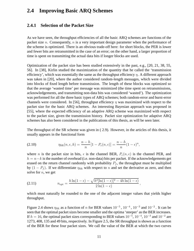
Figure 2.4 showsηSR as a function ofn for BER values10−5 , 10−4 , 10−3 and10−2 . It can beseen that the optimal packet sizes become smaller and the optima ‘steeper’ as the BER increases.If h = 16, the optimal packet sizes corresponding to BER values10−5, 10−4, 10−3 and10−2 are1273, 408, 135 and 49 bits, respectively. In Figure 2.5, the SR throughput is shown as a functionof the BER for these four packet sizes. We call the value of theBER at which the two curves

11

0 500 1000 15000

0.1

0.2

0.3

0.4

0.5

0.6

0.7

0.8

0.9

1

Packet size in bits

SR

thro

ughp

ut η

SR

ε =10−2

ε =10−3

ε =10−4

ε=10−5

Figure 2.4: The SR throughput as a function of packet size with four different BER values whenh = 16 andPf = 0.02

corresponding to packet sizesn1 andn2 intersect thecrossover BERof these packet sizes. Inparticular, ifn1 = 2n2 , then the crossover BER is given by [P4]

(2.12) ǫco = 1 −[

2(n2 − h)

2n2 − h

]1/n2

.

2.4.2 Use of Multicopy Transmissions

Another potential method of improving the performance of the basic ARQ schemes in poorchannel conditions is to use multicopy transmissions, where multiple copies of each data blockare sent contiguously before moving on to the next block in schedule. If at least one of thecopies is received successfully, the data block is acknowledged positively.

For the SR scheme, the throughput would actually decrease ifmulticopy transmissions wereused because then some successful transmissions would be wasted, which does not happenin the basic SR scheme. However, if the buffer space at the receiver is severely limited, theprobability of buffer overflow can be decreased by sending multiple copies of the packet inthe retransmissions. A modified SR scheme based on this idea was proposed and analyzed byWeldon in [75]. If the delay performance is considered instead of throughput, it was shown in[80] that in some burst-error channels the mean transmission delay of a packet in the SR schemecan be reduced by sending two identical copies of the packet separated by a fixed delay at eachtransmission attempt.

12

10−6

10−5

10−4

10−3

10−2

10−1

0

0.1

0.2

0.3

0.4

0.5

0.6

0.7

0.8

0.9

1

BER

SR

thro

ughp

ut, η

SR

n=1273

n=49

n=135

n=408

Figure 2.5: The SR throughput as a function of the BER with four different packet sizes whenh = 16 andPf = 0

In the publications of this thesis, multicopy transmissions are considered with the GBN scheme.An early related work was [64], where Sastry suggested a modified GBN scheme in which, aftera retransmission request, the same data block is sent repeatedly until an ACK is received for it.GBN schemes with multicopy transmissions have also been studied e.g., in [9, 10]. The delayperformance of multicopy GBN schemes was studied in [22]. In[10], the authors showed thatif the GBN ARQ scheme is used in a stationary channel with random packet errors, then theoptimal strategy, which maximizes the packet throughput, is to use the same numberm of copiesin all transmission attempts of a data block. The optimal value ofm, however, depends on thePER and the round-trip delay.

If the PER isPe and feedback errors occur randomly with probabilityPf , then the packetthroughput of them-copy GBN scheme is given by [79]

(2.13) TGBN(N, m, Pe, Pf) =1−[1−(1−Pe)(1−Pf)]

m

m+(N−1)[1−(1−Pe)(1−Pf)]m.

Figure 2.6 showsTGBN as a function of the PER form = 1, 2, 3, 4 whenN = 10 andPf = 0.It can be seen that the performance can be improved significantly by selecting the value ofmoptimally based on channel state information. The PER valueat which the curves correspondingto m = m1 andm = m2 intersect is called thecrossover PER.In the interesting particular case

13

wherem1 = 1 andm2 = 2, the crossover PER can be shown to be [P6]

(2.14) Pco =1N− Pf

1 − Pf.

0 0.1 0.2 0.3 0.4 0.5 0.6 0.7 0.8 0.9 10

0.1

0.2

0.3

0.4

0.5

0.6

0.7

0.8

0.9

1

PER

Pac

ket t

houg

hput

m=1

m=2

m=3

m=4

Figure 2.6: Comparison ofm-copy GBN schemes with different values ofm

2.5 Hybrid ARQ and Packet Combining

The combinations of ARQ schemes and FEC are known as hybrid ARQ (HARQ) schemes[43, 77]. These schemes are further classified into type-I (HARQ-I) and type-II (HARQ-II)schemes.

2.5.1 HARQ-I Schemes

In HARQ-I schemes, all the transmission attempts of a packetare identical codewords contain-ing redundant bits for both error detection and error correction. There are two different ways

14

to accomplish this. In the early HARQ-I schemes, such as those studied in [65, 66], one blockcode was used simultaneously for error detection and error correction. Another approach is touse two codes: an inner code, which is used for error correction (and possibly for simultaneouserror detection if it is a block code), and an outer code, which is used for error detection only.This kind of HARQ-I schemes which use concatenated coding and hence require two encodersat the transmitter and two decoders at the receiver have beenproposed and analyzed for examplein [8, 24, 36].

Generally speaking, the HARQ-I schemes are best suited for channel environments where thelevel of noise and interference is fairly constant. Then theerror-correcting capability of theFEC part of the scheme can be designed so that most of the erroneously received words can becorrected, which reduces the number of retransmissions. However, in time-varying channels,these schemes lack flexibility in adapting to changing channel conditions: the additional paritybits for error correction may represent a waste of bandwidthwhen the channel BER is low forlong periods of time; on the other hand, the designed error-correcting capability may not besufficient for the occasional noisy periods.

2.5.2 HARQ-II Schemes

The adaptivity which is desired in time-varying channel environments is achieved to some extentby HARQ-II schemes, where the parity bits for error correction are sent only when they areneeded. This is known as the method of incremental redundancy, the concept of which was firstintroduced by Mandelbaum in [51]. On the first transmission attempt, only parity bits for errordetection are appended to the message, in the same way as in basic ARQ schemes. If errorsare detected in the received word, it is stored in a buffer anda retransmission is requested. Theretransmission is not the original codeword but a block of parity-check bits formed based onthe original message and an error-correcting code. When this block is received, it is used tocorrect the errors in the previously stored erroneous word.If the error correction fails, anotherretransmission is requested, which can be either a repetition of the original codeword or anotherparity block, depending on the retransmission strategy andthe type of error-correcting code thatis used. This process continues until the original codewordis delivered successfully. One of thefirst articles to describe a scheme using incremental redundancy was [53], where Reed-Mulleror convolutional codes were used for error correction.

Probably the most widely known HARQ-II scheme, and the first scheme to be called by thatname, was proposed and analyzed in a BSC environment in [45] and improved in [74]. Inthis scheme, a rate-1/2 invertible block code or a rate-1/2 convolutional code is used for errorcorrection. In the retransmissions, the original codewordand the parity block alternate, but onlytwo packets are combined at a time to retrieve the original message. Throughput analysis of thisscheme in a packet-level G-E channel was done in [48]. In [78], Yang and Bhargava studiedthe delay and coding gain performance of a ‘truncated’ HARQ-II scheme where at most oneretransmission per packet is allowed, and in [50], Malkamaki and Leib studied the performanceof truncated HARQ-II schemes in block fading channels.

The generalization of this idea to combination of more than two packets is known as code com-bining and was first suggested by Chase in [17], and the throughput performance of an HARQ-

15

II scheme using code combining was studied by Kallel in [34].This type of schemes are oftencalled generalized HARQ-II schemes.In [57], Mukhtar et al. analyzed both the throughputand the delay performance of a scheme with three ‘stages’ of code combining, and more gen-eral expressions for the mean transfer delay of anM-stage generalized HARQ-II scheme wereobtained in [41] by using signal flow graphs.

In the recent years, numerous HARQ-II schemes have been proposed using advanced codingtechniques, such as trellis-coded modulation [23], turbo coding [58] and zigzag codes [16].

If the packet combining is done after the quantization of thereceived data into bits, we have ahard combiningsystem. Lately, there has been a substantial interest in HARQ schemes usingsoft combiningmethods. In [31], for example, the authors study a scheme where several erro-neously received copies of a codeword are concatenated (without hard symbol quantization intobits) to form a noise-corrupted codeword in a longer, lower-rate code. The proposed soft com-bining method is obtained by using now the symbol-by-symbolMAP (maximum a posteriori)decoder for the aforementioned longer code.

2.5.3 Diversity Combining

Besides code combining, which is used in HARQ-II schemes, analternative way of combiningpackets is to use diversity combining, where multiple identical (except for the errors) copies ofa packet are combined to locate the errors [77, p. 394]. One such technique is to compute thebitwise modulo-2 sum (or logical XOR) of two received erroneous copies of a packet and touse the resulting ‘joint bit error map’ to retrieve the original message. This method was firstproposed in [67], and the throughput analysis of an ARQ scheme with packet combining basedon this idea was presented in [P1]. A ‘softer’ form of Sindhu’s combining method was proposedby Benelli in [7], where four-level quantization was performed on the received packets beforecombining. In [1], Adachi et al. studied a time diversity ARQscheme which used maximalratio combining (MRC) at the receiver, and in [76], Wicker added a majority-logic diversitycombiner to a HARQ-I scheme to reduce the retransmissions.

2.6 Adaptive ARQ

By an adaptive ARQ scheme, we mean an ARQ scheme with two or more different transmissionmodes meant for different channel conditions, which uses some channel sensing mechanismto decide which transmission mode is used. A change of transmission mode can mean, forexample, a change of the packet size in the SR scheme (e.g., [52]), or a change of the numberof transmitted copies of a packet in the GBN scheme (e.g., [79]), or a change of the code ratein an HARQ-I scheme (e.g., [60]). In these schemes, the channel sensing is usually done byobserving the acknowledgements sent by the receiver to the transmitter. This can mean eitherestimation of error rates, as in [52], or detection of channel state changes, as in [61] and [79],which does not require as long an observation interval (OBI)as reliable error rate estimation.

16

In [52], an adaptive SR scheme was proposed, where the packetsize used in the current trans-mission was selected from a finite set of values based on a long-term BER estimate. Thisestimate was obtained by counting the incorrectly receivedpackets over a time interval and as-suming that there can be at most one bit error in an erroneous packet. Another adaptive SRscheme with variable packet size was proposed in [55], wherethe a posterioridistribution ofthe BER was computed based on the number of retransmissions during the OBI, and the packetsize was selected so that the expected efficiency of the protocol was maximized. In [29], anadaptive SW scheme with variable packet size was proposed and simulated in a fading chan-nel environment. The selection of the packet size was based on the PER estimate obtained byobserving the acknowledgements over an OBI.

In [79], Yao proposed an adaptive GBN scheme where the transmitted number of copies of apacket was variable. The channel sensing algorithm suggested by Yao is used also in [P2]–[P6]and will be described in Section 3.1. Another adaptive GBN scheme was proposed in [39].In this scheme, there areN transmission modes corresponding to the numbers of transmittedcopies1, . . . , N . The transmission mode is changed when a possible change of the channel stateis detected.

Numerous adaptive HARQ schemes have been suggested in the literature. Typically, the coderate is varied according to the estimated channel conditions. In [72] and [73], adaptive HARQ-Ischemes were studied with convolutional codes used for error correction. Finite-state Markovmodels were assumed for the channel. Switching between transmission modes depended on thenumber of erroneous blocks occurring during an OBI. A similar adaptive HARQ-I scheme witheither block or convolutional codes was proposed in [60]. In[61], sequential statistical testswere applied on the acknowledgements to detect channel state changes. An adaptive HARQ-IIscheme with variable packet size was proposed for wireless ATM networks in [33]. This schemeused rate compatible convolutional (RCC) codes for error correction. In [19], three differentadaptive HARQ schemes are proposed using Reed-Solomon codes for error correction. Anotheradaptive HARQ scheme using Reed-Solomon codes with variable rate for error correction wasproposed in [54]. In this scheme, short-term symbol error rate was estimated by computingthe bitwise modulo-2 sum of two erroneous copies of a packet.This method was originallyproposed in [15].

17

18

Chapter 3

Adaptive ARQ Schemes Based on Yao’sAlgorithm

3.1 Yao’s Channel Sensing Algorithm

In [79], Yao proposed an adaptive GBN scheme with two transmission modes,L andH, meantfor ‘good’ and ‘bad’ channel conditions, respectively. Mode L is the standard GBN scheme,but in modeH, m copies of the packet are sent at each transmission attempt. Switching be-tween transmission modes is done based on the following simple algorithm: in modeL, if thetransmitter receivesα contiguous NACKs, it switches to modeH and begins multicopy trans-missions. If the transmitter receivesβ contiguous ACKs in modeH, it switches immediatelyback to modeL.

3.2 Related Work

It was noted in [3, 13] that the simple two-state Markov chainused by Yao [79] in his analysisdid not model the dynamics of the adaptive GBN scheme with sliding OBIs correctly, evenin a stationary channel. Instead, a Markov chain withα + β states was needed. In [12], aslightly different adaptive GBN scheme with static OBIs of lengthsα andβ was modelled by atwo-state semi-Markov process, still assuming a stationary channel environment. In [4], Yao’salgorithm was applied to an adaptive SR scheme with variablepacket size in stationary fadingchannels. Optimization ofα andβ for stationary channels has been studied in [3, 5] for anadaptive GBN scheme in a BSC environment, and in [4] for an adaptive SR scheme in a fadingchannel environment using the threshold model.

19

3.3 System Model and Throughput Analysis

In publications [P2]–[P6] of this thesis, the dynamics of the system consisting of the time-varying channel environment and the adaptive ARQ scheme aremodelled in a straightforwardfashion by Markov chains. The states of these processes are characterized by the state of theforward channel (G or B), (possibly) the state of the return channel (g or b), the transmissionmode (L or H), and the state of the counter of contiguous NACKs in modeL (0, . . . , α − 1) orthe counter of contiguous ACKs in modeH (0, . . . , β − 1). The number of the states dependson the feedback channel model and on the values of the design parametersα andβ.

In [P2]–[P5], we have studied adaptive SR schemes, were packet sizes ofn1 andn2 bits, wheren1 = 2n2, are used in transmission modesL andH, respectively. The number of parity bits forerror detection,h, is the same in both the cases. The receiver sends the acknowledgements tothe transmitter always after receivingn1 bits. In theH mode, this means acknowledging pairsof n2-bit packets; still, only the incorrectly receivedn2-bit packets are retransmitted. Thesedefinitions make the scheme easy to implement. Switching between transmission modes is donebased on a slightly modified version of Yao’s algorithm: in modeL, if the transmitter receivesαNACKs contiguously, it switches immediately to modeH; in modeH, afterβ contiguous pairsof n2-bit packets have been received completely free of errors and acknowledged positively,modeL is resumed. In the simplest case, as in [P2] and [P3], the return channel is assumed tobe error-free and the round-trip delay is assumed to be negligible. Then the system model has2(α + β) states, which are defined as follows:

(i) States1, . . . , α, also denoted byGLr, wherer = 0, . . . , α − 1: the channel state isG,the transmission mode isL, and the transmitter has receivedr contiguous NACKs. Thesestates form the groupGL.

(ii) Statesα + 1, . . . , α + β, also denoted byGHr, wherer = 0, . . . , β − 1: the channel stateis G, the transmission mode isH, and the transmitter has receivedr contiguous ‘doubleACKs’. These states form the groupGH.

(iii) Statesα + β + 1, . . . , 2α + β, also denoted byBLr, wherer = 0, . . . , α − 1: these statesform the groupBL and are similar to the statesGLr, except that the channel is in stateB.

(iv) States2α + β + 1, . . . , 2(α + β), also denoted byBHr, wherer = 0, . . . , β − 1: thesestates form the groupBH and are similar to the statesGHr, except that the channel is instateB.

The non-zero transition probabilities are given in Table 3.1. In the table entries,PCG andPCB

denote the probabilities of a correct transmission in statesG andB, respectively. The transitionprobabilities of the forward channel fromG to B and fromB to G are denoted byγ andδ,respectively, as was mentioned earlier in Section 2.1.1.

Figure 3.1 shows the state transition diagram for this system model whenα = 2 andβ = 3.

20

Table 3.1: The non-zero transition probabilities of the system model in [P2]old state new state probability

GLi, 0 ≤ i ≤ α − 2

GL0 (1 − γ)PCG

GLi+1 (1 − γ)(1 − PCG)BL0 γPCG

BLi+1 γ(1 − PCG)

GLα−1

GL0 (1 − γ)PCG

GH0 (1 − γ)(1 − PCG)BL0 γPCG

BH0 γ(1 − PCG)

GHi, 0 ≤ i ≤ β − 2

GH0 (1 − γ)(1 − PCG)GHi+1 (1 − γ)PCG

BH0 γ(1 − PCG)BHi+1 γPCG

GHβ−1

GL0 (1 − γ)PCG

GH0 (1 − γ)(1 − PCG)BL0 γPCG

BH0 γ(1 − PCG)

BLi, 0 ≤ i ≤ α − 2

GL0 δPCB

GLi+1 δ(1 − PCB)BL0 (1 − δ)PCB

BLi+1 (1 − δ)(1 − PCB)

BLα−1

GL0 δPCB

GH0 δ(1 − PCB)BL0 (1 − δ)PCB

BH0 (1 − δ)(1 − PCB)

BHi, 0 ≤ i ≤ β − 2

GH0 δ(1 − PCB)GHi+1 δPCB

BH0 (1 − δ)(1 − PCB)BHi+1 (1 − δ)PCB

BHβ−1

GL0 δPCB

GH0 δ(1 − PCB)BL0 (1 − δ)PCB

BH0 (1 − δ)(1 − PCB)

The performance of an adaptive ARQ scheme is measured here byits average throughput, whichis defined as the average of the throughput of the scheme over all the states of the system model.For example, the average throughput of the adaptive SR scheme in [P2] is given by

ηadapt =ηSR(n1, ǫ1, h) ·∑

i∈GL

πi + ηSR(n2, ǫ1, h) ·∑

i∈GH

πi+

ηSR(n1, ǫ2, h) ·∑

i∈BL

πi + ηSR(n2, ǫ2, h) ·∑

i∈BH

πi ,(3.1)

where for example,∑

i∈GL πi is the probability that the forward channel is in stateG and thetransmission mode isL, andηSR(n1, ǫ1, h) is the corresponding throughput, and so on.

21

GL0

GL1

9

8

7

6

5

4

2

1

10

3

BH2

BH1

BH0

BL1

BL0

GH2

GH1

GH0

Figure 3.1: The state transition diagram of the system modelin [P2] and [P3] whenα = 2 andβ = 3

The average throughput of a ‘real’ scheme (specified by the values ofα andβ) is upper-boundedby that of an ideal adaptive scheme, which is always in the ‘correct’ transmission mode. Thatis, the time periods when the forward channel is in stateG coincide with those when the trans-mission mode isL. In [P2], this upper bound is given by

(3.2) ηideal = πG · ηSR(n1, ǫ1, h) + πB · ηSR(n2, ǫ2, h) ,

where the functionηSR(n, ǫ, h) was defined in ( 2.10), andπG andπB are the steady-state prob-abilities of the forward channel being in statesG andB, respectively.

In [P4], the round-trip delay was also assumed to be negligible, but a G-E model was nowassumed also for the return channel. The state of the total system consisting of the adaptiveSR scheme and the two channels develops in time according to aMarkov chain with4(α + β)states, which are defined as follows:

(i) States1, . . . , α , also denoted byGgLr , wherer = 0, . . . , α − 1: the forward and returnchannel states areG andg , respectively, the transmission mode isL , and the transmitterhas receivedr contiguous NACKs. These states form the groupGgL .

(ii) Statesα + 1, . . . , α + β , also denoted byGgHr , wherer = 0, . . . , β − 1: the forwardand return channel states areG andg , respectively, the transmission mode isH , and thetransmitter has receivedr contiguous double-ACKs. These states form the groupGgH .

22

(iii) Statesα+β +1, . . . , 2α+β , also denoted byGbLr , wherer = 0, . . . , α−1: these statesform the groupGbL and are similar to the statesGgLr , except that the return channel isin stateb .

(iv) States2α + β + 1, . . . , 2(α + β) , also denoted byGbHr , wherer = 0, . . . , β − 1: thesestates form the groupGbH and are similar to the statesGgHr , except that the returnchannel is in stateb .

(v) States2(α + β) + 1, . . . , 3α + 2β , also denoted byBgLr , wherer = 0, . . . , α− 1: thesestates form the groupBgL and are similar to the statesGgLr , except that the forwardchannel is in stateB .

(vi) States3α + 2β + 1, . . . , 3(α + β) , also denoted byBgHr , wherer = 0, . . . , β − 1: thesestates form the groupBgH and are similar to the statesGgHr , except that the forwardchannel is in stateB .

(vii) States3(α + β) + 1, . . . , 4α + 3β , also denoted byBbLr , wherer = 0, . . . , α − 1: thesestates form the groupBbL and are similar to the statesGbLr , except that the forwardchannel is in stateB .

(viii) States4α + 3β + 1, . . . , 4(α + β) , also denoted byBbHr , wherer = 0, . . . , β − 1: thesestates form the groupBbH and are similar to the statesGbHr , except that the forwardchannel is in stateB .

The transitions between the states of the system model happen at regular time intervals corre-sponding ton1 transmitted bits. They are determined by

• state transitions of the two channels,

• success/failure of the transmission of the current packet,

• correctness of the corresponding received, acknowledgement (this is relevant only whenthe return channel is in stateb).

The number of possible state transitions from one state of the system model is either 8 or 12,depending on the possibility and consequences of a feedbackerror. Note that in the precedingcase of error-free return channel, there were only 4 possible transitions from each state.

It is very difficult to draw a complete state transition diagram of the system model clearly, evenwith smallα andβ. However, there is a lot of symmetry in the model. The set of states canbe divided into four subsets in a very natural way based on thechannel state combinations. Wedenote these subsets byGg , Gb , Bg andBb .

Table 3.2 shows the non-zero transition probabilities for two groups of states,GgL andBbH .In the table entries,Pe,1 andPe,2 are the probabilities that there is at least one bit error in a

23

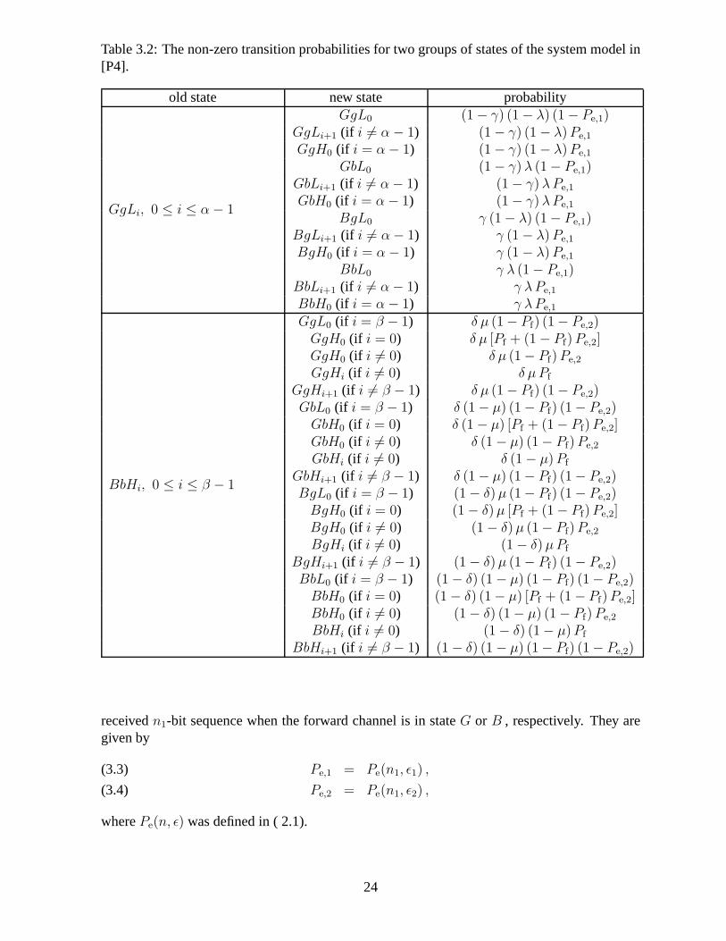
Table 3.2: The non-zero transition probabilities for two groups of states of the system model in[P4].

old state new state probability

GgLi, 0 ≤ i ≤ α − 1

GgL0 (1 − γ) (1 − λ) (1 − Pe,1)GgLi+1 (if i 6= α − 1) (1 − γ) (1 − λ) Pe,1

GgH0 (if i = α − 1) (1 − γ) (1 − λ) Pe,1

GbL0 (1 − γ) λ (1 − Pe,1)GbLi+1 (if i 6= α − 1) (1 − γ) λ Pe,1

GbH0 (if i = α − 1) (1 − γ) λ Pe,1

BgL0 γ (1 − λ) (1 − Pe,1)BgLi+1 (if i 6= α − 1) γ (1 − λ) Pe,1

BgH0 (if i = α − 1) γ (1 − λ) Pe,1

BbL0 γ λ (1 − Pe,1)BbLi+1 (if i 6= α − 1) γ λ Pe,1

BbH0 (if i = α − 1) γ λ Pe,1

BbHi, 0 ≤ i ≤ β − 1

GgL0 (if i = β − 1) δ µ (1 − Pf) (1 − Pe,2)GgH0 (if i = 0) δ µ [Pf + (1 − Pf) Pe,2]GgH0 (if i 6= 0) δ µ (1 − Pf) Pe,2

GgHi (if i 6= 0) δ µ Pf

GgHi+1 (if i 6= β − 1) δ µ (1 − Pf) (1 − Pe,2)GbL0 (if i = β − 1) δ (1 − µ) (1 − Pf) (1 − Pe,2)

GbH0 (if i = 0) δ (1 − µ) [Pf + (1 − Pf) Pe,2]GbH0 (if i 6= 0) δ (1 − µ) (1 − Pf) Pe,2

GbHi (if i 6= 0) δ (1 − µ) Pf

GbHi+1 (if i 6= β − 1) δ (1 − µ) (1 − Pf) (1 − Pe,2)BgL0 (if i = β − 1) (1 − δ) µ (1− Pf) (1 − Pe,2)

BgH0 (if i = 0) (1 − δ) µ [Pf + (1 − Pf) Pe,2]BgH0 (if i 6= 0) (1 − δ) µ (1− Pf) Pe,2

BgHi (if i 6= 0) (1 − δ) µ Pf

BgHi+1 (if i 6= β − 1) (1 − δ) µ (1− Pf) (1 − Pe,2)BbL0 (if i = β − 1) (1 − δ) (1 − µ) (1 − Pf) (1 − Pe,2)

BbH0 (if i = 0) (1 − δ) (1 − µ) [Pf + (1 − Pf) Pe,2]BbH0 (if i 6= 0) (1 − δ) (1 − µ) (1 − Pf) Pe,2

BbHi (if i 6= 0) (1 − δ) (1 − µ) Pf

BbHi+1 (if i 6= β − 1) (1 − δ) (1 − µ) (1 − Pf) (1 − Pe,2)

receivedn1-bit sequence when the forward channel is in stateG or B , respectively. They aregiven by

Pe,1 = Pe(n1, ǫ1) ,(3.3)

Pe,2 = Pe(n1, ǫ2) ,(3.4)

wherePe(n, ǫ) was defined in ( 2.1).

24

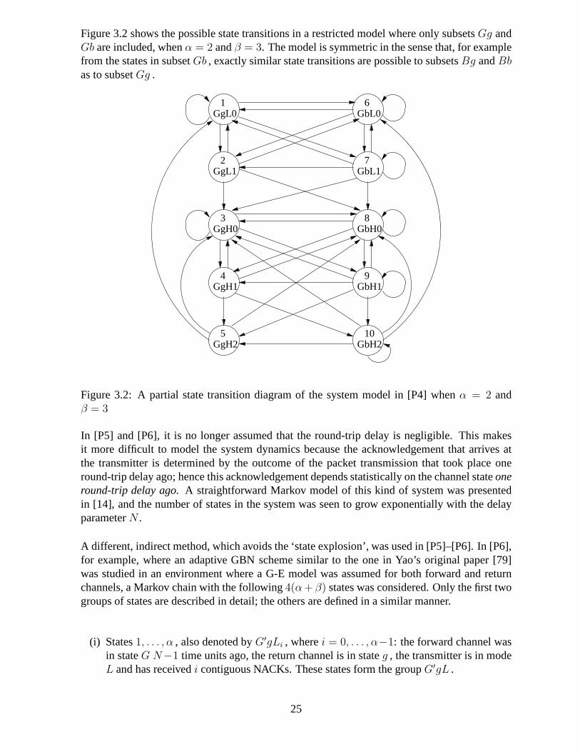
Figure 3.2 shows the possible state transitions in a restricted model where only subsetsGg andGb are included, whenα = 2 andβ = 3. The model is symmetric in the sense that, for examplefrom the states in subsetGb , exactly similar state transitions are possible to subsetsBg andBbas to subsetGg .

GbH2

GbH1

GbH0

GbL1

GbL0

GgH2

GgH1

GgH0

GgL1

GgL0

9

8

7

6

5

4

2

1

10

3

Figure 3.2: A partial state transition diagram of the systemmodel in [P4] whenα = 2 andβ = 3

In [P5] and [P6], it is no longer assumed that the round-trip delay is negligible. This makesit more difficult to model the system dynamics because the acknowledgement that arrives atthe transmitter is determined by the outcome of the packet transmission that took place oneround-trip delay ago; hence this acknowledgement depends statistically on the channel stateoneround-trip delay ago.A straightforward Markov model of this kind of system was presentedin [14], and the number of states in the system was seen to growexponentially with the delayparameterN .

A different, indirect method, which avoids the ‘state explosion’, was used in [P5]–[P6]. In [P6],for example, where an adaptive GBN scheme similar to the one in Yao’s original paper [79]was studied in an environment where a G-E model was assumed for both forward and returnchannels, a Markov chain with the following4(α + β) states was considered. Only the first twogroups of states are described in detail; the others are defined in a similar manner.

(i) States1, . . . , α , also denoted byG′gLi , wherei = 0, . . . , α−1: the forward channel wasin stateG N−1 time units ago, the return channel is in stateg , the transmitter is in modeL and has receivedi contiguous NACKs. These states form the groupG′gL .

25

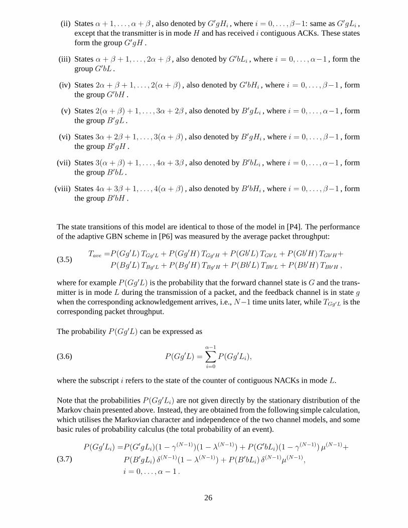
(ii) Statesα + 1, . . . , α + β , also denoted byG′gHi , wherei = 0, . . . , β−1: same asG′gLi ,except that the transmitter is in modeH and has receivedi contiguous ACKs. These statesform the groupG′gH .

(iii) Statesα + β + 1, . . . , 2α + β , also denoted byG′bLi , wherei = 0, . . . , α−1 , form thegroupG′bL .

(iv) States2α + β + 1, . . . , 2(α + β) , also denoted byG′bHi , wherei = 0, . . . , β−1 , formthe groupG′bH .

(v) States2(α + β) + 1, . . . , 3α + 2β , also denoted byB′gLi , wherei = 0, . . . , α−1 , formthe groupB′gL .

(vi) States3α + 2β + 1, . . . , 3(α + β) , also denoted byB′gHi , wherei = 0, . . . , β−1 , formthe groupB′gH .

(vii) States3(α + β) + 1, . . . , 4α + 3β , also denoted byB′bLi , wherei = 0, . . . , α−1 , formthe groupB′bL .

(viii) States4α + 3β + 1, . . . , 4(α + β) , also denoted byB′bHi , wherei = 0, . . . , β−1 , formthe groupB′bH .

The state transitions of this model are identical to those ofthe model in [P4]. The performanceof the adaptive GBN scheme in [P6] was measured by the averagepacket throughput:

Tave =P (Gg′L) TGg′L + P (Gg′H) TGg′H + P (Gb′L) TGb′L + P (Gb′H) TGb′H+

P (Bg′L) TBg′L + P (Bg′H) TBg′H + P (Bb′L) TBb′L + P (Bb′H) TBb′H ,(3.5)

where for exampleP (Gg′L) is the probability that the forward channel state isG and the trans-mitter is in modeL during the transmission of a packet, and the feedback channel is in stategwhen the corresponding acknowledgement arrives, i.e.,N−1 time units later, whileTGg′L is thecorresponding packet throughput.

The probabilityP (Gg′L) can be expressed as

(3.6) P (Gg′L) =

α−1∑

i=0

P (Gg′Li),

where the subscripti refers to the state of the counter of contiguous NACKs in modeL.

Note that the probabilitiesP (Gg′Li) are not given directly by the stationary distribution of theMarkov chain presented above. Instead, they are obtained from the following simple calculation,which utilises the Markovian character and independence ofthe two channel models, and somebasic rules of probability calculus (the total probabilityof an event).

P (Gg′Li) =P (G′gLi)(1 − γ(N−1))(1 − λ(N−1)) + P (G′bLi)(1 − γ(N−1)) µ(N−1)+

P (B′gLi) δ(N−1)(1 − λ(N−1)) + P (B′bLi) δ(N−1)µ(N−1),

i = 0, . . . , α − 1 .

(3.7)

26

The probabilitiesP (Gg′H), P (Gb′L), P (Gb′H), P (Bg′L), P (Bg′H), P (Bb′L) andP (Bb′H)are obtained in a similar way. The corresponding throughputvalues are given by the followingequations

TGg′L = TGBN(N, m1, Pe,1, 0) ,

TGg′H = TGBN(N, m2, Pe,1, 0) ,

TGb′L = TGBN(N, m1, Pe,1, Pf) ,

TGb′H = TGBN(N, m2, Pe,1, Pf) ,

TBg′L = TGBN(N, m1, Pe,2, 0) ,

TBg′H = TGBN(N, m2, Pe,2, 0) ,

TBb′L = TGBN(N, m1, Pe,2, Pf) ,

TBb′H = TGBN(N, m2, Pe,2, Pf) .

(3.8)

An upper bound forTave is provided by the average packet throughput of an ideal adaptiveGBN scheme, where the time periods when the forward channel is in stateG (B) coincidewith those when the transmission mode isL (H). Since the forward and feedback channels areindependent, this upper bound is given by

Tideal =πGπgTGBN(N, m1, Pe,1, 0) + πGπbTGBN(N, m1, Pe,1, Pf)+

πBπgTGBN(N, m2, Pe,2, 0) + πBπbTGBN(N, m2, Pe,2, Pf) .(3.9)

3.4 Parameter Optimization

In [3, 4, 5], the authors presented optimization results forparametersα andβ. An adaptiveSR scheme with variable packet size was considered in [4] in aRayleigh fading environmentusing the threshold model, whereas the two other papers discussed an adaptive GBN schemein a channel environment where packet errors occur randomly. However, none of these articlesused a real time-varying channel model.

A different approach was used in publications [P4]–[P6] of this thesis. In each paper, a G-Echannel model was used to represent a time-varying channel environment. Further, optimizationof the packet size was studied for adaptive SR schemes in [P4]and [P5].

3.4.1 Optimization of the Packet Size

Parameter optimization for the adaptive SR scheme in [P4] and [P5] was done in two steps. First,the packet sizes are optimized for the ‘ideal’ adaptive scheme, and then the optimal packet sizesare adopted when parametersα andβ are being optimized.

In the ‘two-dimensional’ packet size optimization, we let the BER values in forward channelstatesG andB, ǫ1 andǫ2, vary over intervals[ǫ1,a, ǫ1,b] and[ǫ2,a, ǫ2,b], respectively. The schemeuses two different packet sizes,n1 andn2, wheren1 = 2n2. The smaller packet sizen2 is

27

taken as the independent parameter, and the optimal value ofn2 is defined to be the one thatmaximizes the double integral

ǫ1,b∫

ǫ1,a

ǫ2,b∫

ǫ2,a

ηideal(ǫ1, ǫ2; n2) dǫ1dǫ2,

while satisfying the conditionǫ1,b < ǫco < ǫ2,a, whereǫco, the cross-over BER between packetsizesn2 and2n2, is obtained from Eq. 2.12. Maximization of the integral above is equivalent tomaximizing

(3.10) I1(n2) =

ǫ1,b∫

ǫ1,a

ǫ2,b∫

ǫ2,a

[

πG

(

1 − h

2n2

)

(1 − ǫ1)2n2 + πB

(

1 − h

n2

)

(1 − ǫ2)n2

]

dǫ1dǫ2.

In the ‘one-dimensional’ optimization,ǫ1 is fixed and optimization is performed over a range ofǫ2-values, and the integral to be maximized is one-dimensional:

(3.11) I2(n2) =

ǫ2,b∫

ǫ2,a

[

πG

(

1 − h

2n2

)

(1 − ǫ1)2n2 + πB

(

1 − h

n2

)

(1 − ǫ2)n2

]

dǫ2 .

In this case, we require thatǫ1 < ǫco < ǫ2,a .

3.4.2 Optimization ofα and β

In [P4], the following (one-dimensional) approach is used in the optimization ofα andβ. Weuse the value ofn2 that maximizesI2(n2), and define the optimal(α, β)-combination as the onethat minimizes the mean-square difference ofηave andηideal over the interval[ǫ2,a, ǫ2,b]. This isapproximately equivalent to minimizing the sum

(3.12) E(α, β) =K

∑

k=1

[ηave(ǫ2,k; α, β) − ηideal(ǫ2,k)]2,

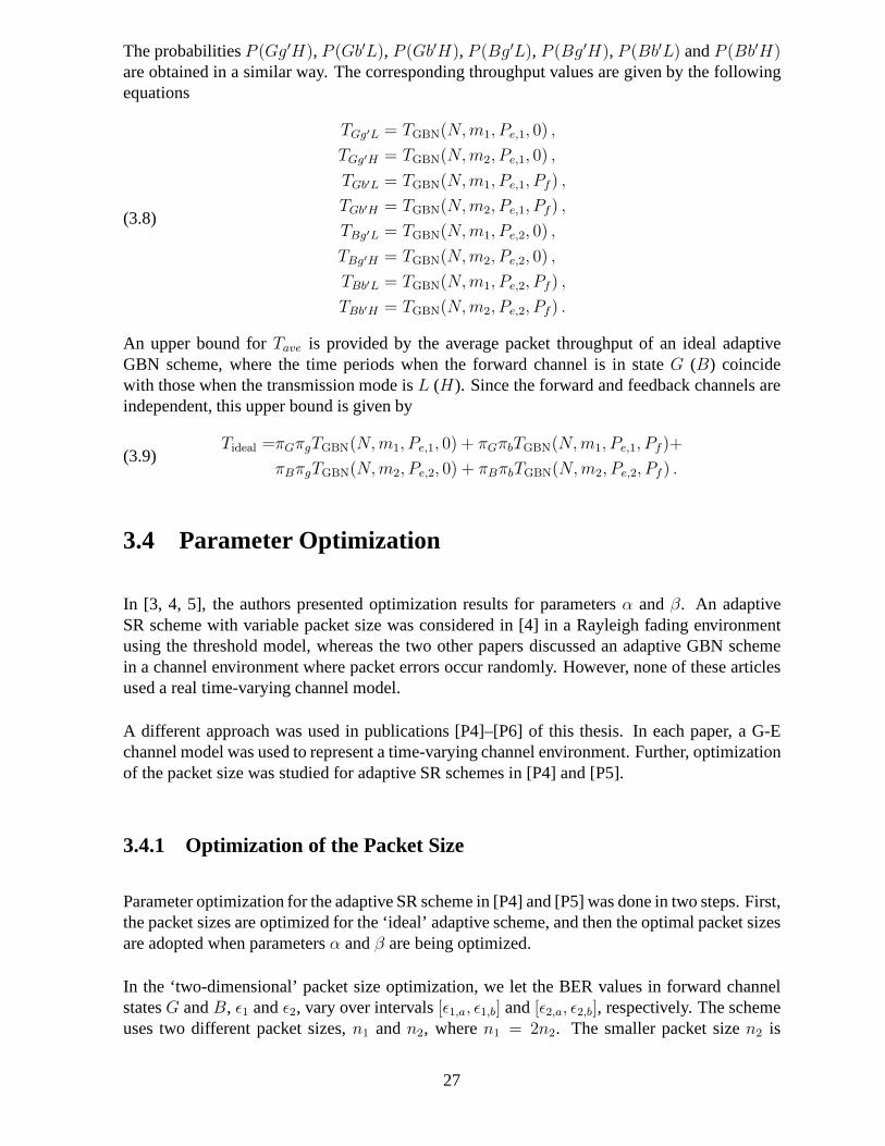
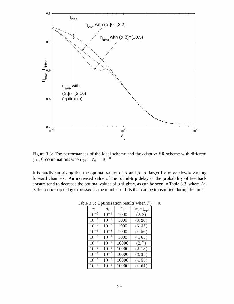
where the sample valuesǫ2,k, k = 1, . . . , K, are evenly spaced on the interval[ǫ2,a, ǫ2,b]. Sincewe do not have a closed-form expression forηave as a function ofα, β and other parameters,a computer search must be used in the optimization. Figure 3.3 shows the average throughputof the adaptive SR scheme in [P4] with different values ofα andβ, and the upper boundηideal,as functions ofǫ2 (the BER in stateB) for a given set of values of the parameters specifyingthe SR scheme. The difference between the ideal curve and theoptimal actual performancecurve corresponding to(α, β) = (2, 16) is at most points too small to be visible. The two otherparameter combinations illustrated here are clearly inferior choices.

3.5 Summary of Optimization Results

The optimal value ofn2 is determined essentially by the proportion of time that theforwardchannel stays in stateB. The smaller the value ofπB is, the bigger is the optimal value ofn2.

28

10−3

10−2

10−1

0.4

0.5

0.6

0.7

0.8

ε2

η ave, η

idea

l

ηideal

ηave

with (α,β)=(2,2)

ηave

with (α,β)=(10,5)

ηave

with

(α,β)=(2,16)(optimum)

Figure 3.3: The performances of the ideal scheme and the adaptive SR scheme with different(α, β)-combinations whenγ0 = δ0 = 10−6

It is hardly surprising that the optimal values ofα andβ are larger for more slowly varyingforward channels. An increased value of the round-trip delay or the probability of feedbackerasure tend to decrease the optimal values ofβ slightly, as can be seen in Table 3.3, whereD0

is the round-trip delay expressed as the number of bits that can be transmitted during the time.

Table 3.3: Optimization results whenPf = 0.γ0 δ0 D0 (α, β)opt

10−5 10−5 1000 (2, 8)10−6 10−6 1000 (3, 26)10−7 10−7 1000 (3, 37)10−8 10−8 1000 (4, 56)10−9 10−9 1000 (4, 65)10−5 10−5 10000 (2, 7)10−6 10−6 10000 (2, 13)10−7 10−7 10000 (3, 35)10−8 10−8 10000 (4, 55)10−9 10−9 10000 (4, 64)

29

30

Chapter 4

ARQ with Diversity Combining

4.1 The EARQ Scheme with Time Diversity

In [67], Sindhu proposed a simple idea of combining incorrectly received packets to recoverthe correct packet. A crucial procedure in this scheme was the computation of the bit-wiseXOR (Exclusive-OR) or, equivalently, the bit-wise modulo-2 sum of two incorrectly receivedversions of a packet. The purpose of this operation was to getinformation about the potentiallocations of the errors in the packets. The analysis in [67] considered only a burst-error channelenvironment. In [P1], this idea has been applied to a simple SR ARQ scheme resulting in whatis called theextended ARQ (EARQ)scheme.

The EARQ scheme uses only one(n, k) code, which is used for error detection only. Thescheme operates as follows. If errors are detected in the first transmission of a codeword, thereceived vector is stored in the receiver buffer and a retransmission is requested. If the retrans-mission is error-free, the received vector is assumed to be the original codeword and an ACK issent to the transmitter. If errors are detected also in the retransmission, the bit-wise XOR of thetwo erroneous copies of the codeword is computed.

The output of the XOR operation is ann-bit vector with 0s in the bit positions where the copiescoincide and 1s in the bit positions where they differ. The positions with 1s are the ones whereexactly one of the copies has an error. If, on the other hand, there is at least one bit positionwhere both copies have an error, this results in a 0 in the output of the XOR operation. Thisevent is called adouble errorin [P1].

The next step is to try to recover the original codeword by a straightforward search procedure.This procedure begins from one of the two copies and starts togo through the potential errorpatterns: the corresponding bits are inverted and the syndrome of the resulting vector is com-puted based on the error-detecting code. This process continues until either a vector with zerosyndrome has been obtained or all the possibilities have been checked without a positive result.In the first case, it is assumed that the correct codeword has been recovered and an ACK is sentto the transmitter, which proceeds to transmit the next codeword. In the second case, a doubleerror has occurred and a NACK is sent requesting second retransmission of the codeword.

31

If the second retransmission is found to be error-free, it isaccepted and an ACK is sent tothe transmitter. If errors are detected, the packet combining procedure is carried out with, ifnecessary, both the earlier received erroneous copies. If one of these operations is successful,an ACK is sent. Otherwise, yet another retransmission is requested. This time, the new copy, iffound erroneous, can be combined with three earlier copies,and so on. The process, of course,continues until the codeword has been received correctly orrecovered by the packet combiningprocedure.

One aspect that deserves special attention is thecomputational complexityof the search processmentioned above. If there aren1 1s in the output of the XOR operation, there arenp = 2n1 − 2potential error patterns, all of which are checked if the search is unsuccessful. It is easy to seethatnp increases very rapidly with the noisiness of the channel. One solution to this problem isto define some limitNmax, as in [P1]: packet combining is not attempted with a pair of packetsif the output of the XOR operation contains more thanNmax 1s.

4.2 Approximate Throughput Analysis

In [P1], the EARQ scheme is analyzed assuming a BSC with BER equal to pe. Further, it isassumed that the round-trip delay is negligible and that theapplied code provides perfect errordetection. The packet throughput of the scheme is obtained from

(4.1) TEARQ =1

E[L],

where the random variableL is defined as the number of transmissions required until a codewordhas been successfully received, and its expectation valueE[L] is naturally obtained from

(4.2) E[L] =∞

∑

L=1

L · P (L) .

Clearly, the probability that one transmission is sufficient is equal toPc = 1 − Pe. ForL > 1,

(4.3) P (L) =

[

1 −L−1∑

r=1

P (r)

]

[

Pc + Pe(1 − αd(L))]

,

whereαd(L) is the conditional probability that, given that all theL copies are erroneous andthat all pairs taken out of the firstL − 1 copies have double errors, theLth copy has a double

32

error with all theL − 1 earlier copies. The exact calculation ofαd(L) gets complicated whenL ≥ 3. For example, whenL = 3, the events of the pairs(1, 2), (1, 3) and(2, 3) having doubleerrors are not independent. However, it turns out that the assumption of ‘independent doubleerrors’ is a good approximation of reality, as demonstratedby the good agreement between thesimulations and theoretical calculations in [P1]. Using the independence assumption, we get

(4.4) αd(L) =

∑nk1=1 · · ·

∑nkL=1 P (k1, . . . , kL) ·

∏

1≤i,j≤Li<j

Pi,j

P Le ·

∏L−1l=2 αd(l)

,

where

(4.5) P (k1, . . . , kL) = P (k1)P (k2) · ·P (kL)

is the joint probability of theL copies havingk1, . . . , kL errors, respectively. Since the BSCmodel is assumed, the numbers of errors in the copies are independent and identically distributedrandom variables with binomial distributions:

(4.6) P (ki) =

(

n

ki

)

pkie (1 − pe)

n−ki .

Further,Pi,j is the probability that two copies withki andkj errors, respectively, have a doubleerror. With the assumption thatk1 + kj ≤ n, it is easy to show that

(4.7) Pi,j = 1 − (n − ki)!(n − kj)!

n!(n − ki − kj)!.

If the parameterNmax is also taken into account, the situation where there are more thanNmax

1s in the output of the XOR operation has the same effect as a double error. Thus, the followingmodification is needed:

(4.8) Pi,j =

{

1 − (n−ki)!(n−kj)!

n!(n−ki−kj)!, if ki + kj ≤ Nmax,

1, if ki + kj > Nmax .

The ‘limited’ EARQ scheme has been simulated with three different values ofNmax using 100-bit packets. Figure 4.1 provides the results from these simulations along with approximatedtheoretical packet throughputs for both ‘limited’ and ‘unlimited’ EARQ schemes. In this case,the probabilitiesP (L) have been computed up toL = 5, andP (6) has been approximated bythe tail distribution. Even withNmax = 10, packet throughput of approximately 33% can beachieved at BER as high as 0.05.

33

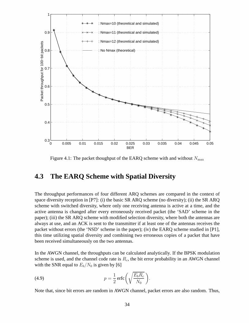
0 0.005 0.01 0.015 0.02 0.025 0.03 0.035 0.04 0.045 0.050.3

0.4

0.5

0.6

0.7

0.8

0.9

1

BER

Pac

ket t

hrou

ghpu

t for

100

−bi

t pac

kets

: Nmax=10 (theoretical and simulated)

: Nmax=11 (theoretical and simulated)

: Nmax=12 (theoretical and simulated)

: No Nmax (theoretical)

Figure 4.1: The packet thoughput of the EARQ scheme with and withoutNmax

4.3 The EARQ Scheme with Spatial Diversity

The throughput performances of four different ARQ schemes are compared in the context ofspace diversity reception in [P7]: (i) the basic SR ARQ scheme (no diversity); (ii) the SR ARQscheme with switched diversity, where only one receiving antenna is active at a time, and theactive antenna is changed after every erroneously receivedpacket (the ‘SAD’ scheme in thepaper); (iii) the SR ARQ scheme with modified selection diversity, where both the antennas arealways at use, and an ACK is sent to the transmitter if at leastone of the antennas receives thepacket without errors (the ‘NSD’ scheme in the paper); (iv) the EARQ scheme studied in [P1],this time utilizing spatial diversity and combining two erroneous copies of a packet that havebeen received simultaneously on the two antennas.

In the AWGN channel, the throughputs can be calculated analytically. If the BPSK modulationscheme is used, and the channel code rate isRc, the bit error probability in an AWGN channelwith the SNR equal toEb/N0 is given by [6]

(4.9) p =1

2erfc

(

√

EbRc

N0

)

.

Note that, since bit errors are random in AWGN channel, packet errors are also random. Thus,

34

the SAD scheme does not provide any benefit over simple SR scheme in AWGN channels.In the NSD scheme, the probability of successfully receiving a packet is that of a successfulreception over either of the diversity branches, that is,

(4.10) P1 = 1 − (1 − (1 − p)n)2,

and the throughput is

(4.11) ηNSD =k

nP1.

In the SR-NSD-EARQ scheme, when both copies are erroneous, apacket is retrieved correctlyif the combined copy does not have a double error, and if the total number of errors in thecombined copy is at mostNmax. The probability that both these conditions are satisfied is

P2 =

Nmax−1∑

k1=1

{(

n

k1

)

pk1(1−p)n−k1 · (1−p)k1

Nmax−k1∑

k2=1

[(

n−k1

k2

)

pk2(1−p)n−k1−k2

]}

=

Nmax−1∑

k1=1

Nmax−k1∑

k2=1

(

n

k1

)(

n−k1

k2

)

pk1+k2(1−p)2n−k1−k2 ,

(4.12)

and the throughput of the EARQ scheme is given by

(4.13) ηEARQ =k

n(P1 + P2).

In Figure 4.2, the throughput curves of these schemes are plotted withk = 84 andn = 100. Itcan be seen that, even withNmax = 4, the EARQ scheme provides considerable performancegain over the other schemes with very reasonable additionalcomputational complexity.

The performances of the four schemes in Rayleigh fading channels are compared by simulationsusing the Jakes model. The throughput curves of the four ARQ schemes as functions of theaverage SNR, whenv = 1 m/s, n = 100 bits, andNmax = 10, are shown in Figure 4.3. Oneobservation that can be made is that the SAD scheme is clearlysuperior to the basic SR schemeover the wide range of SNR considered here. This indicates that the average duration of fadesis fairly long, and the switched antenna diversity improvesthe performance significantly. TheSR-NSD and EARQ schemes can provide further performance improvements.

35

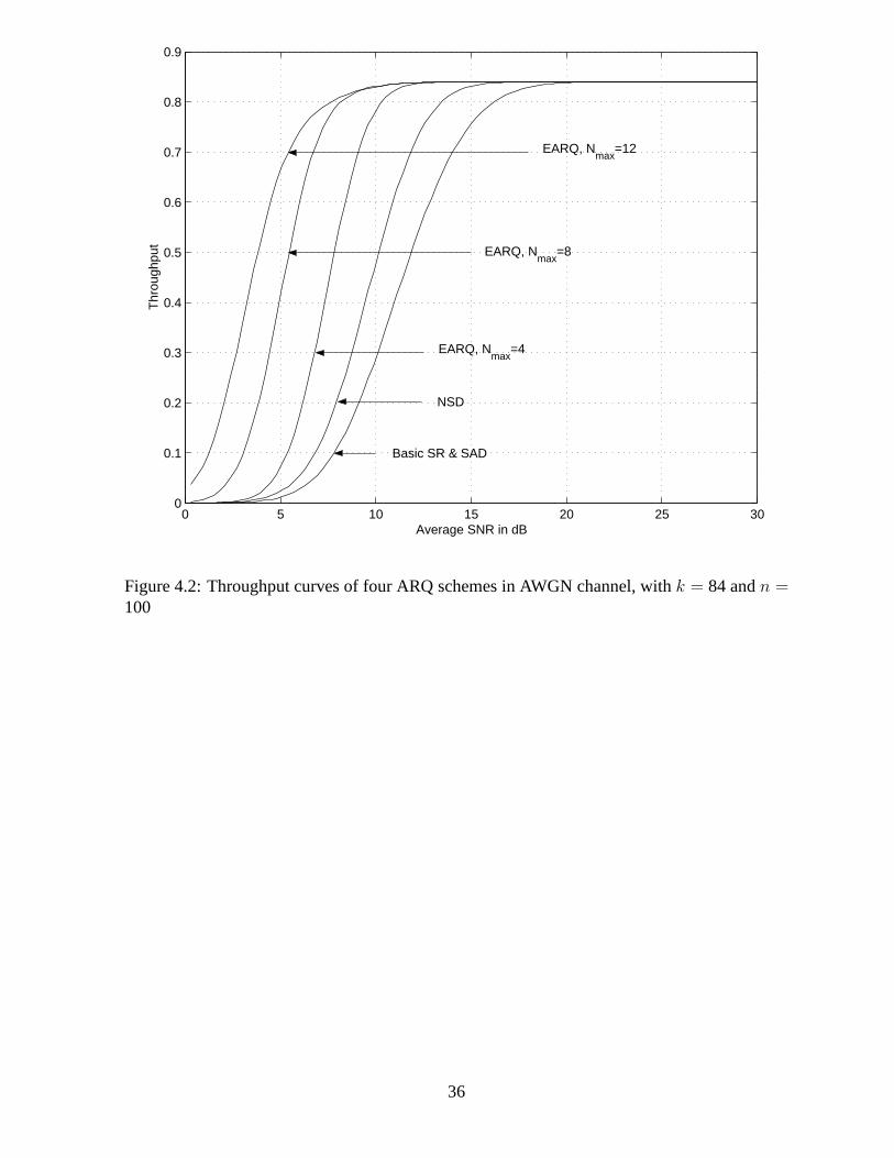
0 5 10 15 20 25 300

0.1

0.2

0.3

0.4

0.5

0.6

0.7

0.8

0.9

Average SNR in dB

Thr

ough

put

Basic SR & SAD

NSD

EARQ, Nmax

=4

EARQ, Nmax

=8

EARQ, Nmax

=12

Figure 4.2: Throughput curves of four ARQ schemes in AWGN channel, withk = 84 andn =100

36

0 5 10 15 20 25 30 35 400

0.1

0.2

0.3

0.4

0.5

0.6

0.7

0.8

0.9

Average SNR in dB

Thr

ough

put

basic SRSAD NSD EARQ

Figure 4.3: Simulated throughputs of the four ARQ schemes when the packet size is 100 bits,v = 1 m/s, andNmax = 10

37

38

Chapter 5

Summary of Publications

In [P1], we present an approximate (packet) throughput analysis and a simulation study of anARQ scheme with packet combining in the stationary BSC environment. The packet combiningalgorithm, where the bitwise modulo-2 sum of two erroneous copies of a packet is computed tolocate the errors, was first proposed by Sindhu in [67]. The validy of the approximate analysisis verified by the good agreement with the simulation results. The packet combining algorithminvolves a straightforward search procedure, the computational complexity of which easily be-comes prohibitive. As a solution to this, a modified scheme isproposed, where the searchprocedure is attempted only when there are at mostNmax 1s at the output of the modulo-2adder. Packet throughput curves of the modified scheme (boththeoretical and simulated) as afunction of the channel BER are shown with various values ofNmax.

Publication [P2] introduces an adaptive SR ARQ scheme with two transmission modes, modeL for ‘good’ and modeH for ‘bad’ channel conditions. In modeL, the packet size isn1

and in modeH n2 bits, wheren1 = 2n2. The smaller packets are acknowledged in pairsby sending ‘bitmaps’ to the transmitter. The switching between the two transmission modesis done according to the algorithm introduced by Yao in [79]:in modeL, if the transmitterreceivesα NACKs contiguously, it switches immediately to modeH and starts to transmitsmaller packets; if the transmitter is in modeH and receivesβ ‘double ACKs’ contiguously, itswitches to modeL. The round-trip delay is assumed to be negligible, and the return channelis assumed to be error-free. The time-varying forward channel is represented by a packet-levelG-E model, where the statesG andB are defined by the BER valuesǫ1 andǫ2, respectively,whereǫ2 ≫ ǫ1. The system is modelled by a Markov chain with2(α+β) states, and the averagethroughput of the adaptive SR scheme is obtained as the time average of the throughput over thestates of the Markov model. As a basis of comparison, we definea hypothetical ideal adaptivescheme which knows the channel state and chooses the transmission mode accordingly: whenthe forward channel is in stateG (B), the transmission mode isL (H). For all the values of thedesign parametersα andβ, the average throughput of the adaptive scheme is upper-bounded bythat of the ideal scheme.

In [P3], the same adaptive SR scheme is studied as in [P2], andthe assumptions about the returnchannel and the round-trip delay are the same. However, the states of the forward channelmodel represent now Rayleigh fading channels defined by the values of the parametersρ and

39

fD according to the threshold model described in Section 2.1.2. The performance analysis isvery similar to that presented in [P2].

The same adaptive SR scheme is also studied in [P4], and the round-trip delay is still assumedto be negligible. The time-varying forward channel is now represented by a bit-level G-E modelso that the channel model is defined independently of the packet size, and this time a G-E modelis assumed also for the return channel: stateg is error-free, and in stateb an acknowledgment iserased with probabilityPf . The system model has now4(α + β) states. In this paper, we alsostudy optimization of the 3 independent design parameters of the adaptive SR scheme:n2, αandβ. This is done in two steps. First we try to find the best possible value ofn2 by optimizingthe performance of the ideal scheme. Then we fixn2 and optimizeα andβ by minimizing(approximately) the mean-square difference between the ideal and actual performance curves(or ‘surfaces’ in the case of two-dimensional optimization). Probably the most important ob-servation of this article is the importance of the judiciousselection of the value ofn2 for theperformance of the adaptive scheme.

Publication [P5] also studies analysis and optimization ofthe same adaptive SR scheme. Theforward channel model is the same as in [P4], but now the acknowledgments are assumed tobe erased randomly with probabilityPf in the return channel. The important difference fromthe earlier articles is that the round-trip delay is no longer assumed to be negligible. The state-space explosion with the increasing delay, which was encountered by the authors in an earlierwork [14], is avoided by using a modified Markov model, which has always2(α + β) statesirrespective of the round-trip delay. The optimal value ofβ is seen to depend slightly on thevalues of the round-trip delay andPf .

In [P6], an adaptive GBN scheme using Yao’s algorithm is analyzed and optimized. The twotransmission modesL andH correspond tom1-copy andm2-copy GBN schemes, respectively.In all the numerical examples, we have setm1 = 1. A packet-level G-E model is assumedfor the forward channel, where the statesG andB are characterized by the PER valuesPe,1

andPe,2, with Pe,2 ≫ Pe,1. A similar model is assumed also for the return channel: state g iserror-free, and in stateb the acknowledgments are erased with probabilityPf . The performanceof the adaptive scheme is measured by its average packet throughput over the4(α + β) statesof the system model, and the optimization ofα andβ is carried out in the same manner as in[P4] and [P5]. The paper also contains a brief discussion of how the burstiness of the forwardchannel errors affects the performance of the adaptive GBN scheme.

Publication [P7] is about ARQ and spatial diversity. The communication system consists of onetransmitting antenna and two receiving antennas. The two diversity branches are assumed tobehave like two independent flat Rayleigh fading channels, which are simulated by using theJakes model. The BPSK modulation scheme is used with coherent demodulation. We comparethe simulated throughput performance of four different ARQschemes: (i) the basic SR ARQscheme (no diversity); (ii) the SR ARQ scheme with switched diversity, where only one receiv-ing antenna is active at a time, and the active antenna is changed after every erroneously receivedpacket; (iii) the SR ARQ scheme with modified selection diversity, where both the antennas arealways at use, and an ACK is sent to the transmitter if at leastone of the antennas receives thepacket without errors; (iv) the EARQ scheme studied in [P1],this time utilizing spatial diversityand combining two erroneous copies of a packet that have beenreceived simultaneously on thetwo antennas. The theoretical throughput performances of the schemes in the AWGN channel

40

are also compared. The main contribution of this article is to present the EARQ scheme as apotential method of choice for systems using spatial diversity reception.

41

42

Chapter 6

Conclusions

In publications [P2–P6] of this thesis, adaptive ARQ schemes based on Yao’s channel sensingalgorithm have been analyzed and optimized in Gilbert-Elliott channels. There are two kindsof non-ideal behaviour that make the throughput curves of the adaptive ARQ schemes deviatefrom those of the ideal schemes. Firstly, there is delay in reacting to changes in the channelstate. This delay becomes of course longer if the values ofα andβ are bigger. Secondly, ‘falsealarms’ occur, making the scheme switch between transmission modes unnecessarily. Here,bigger values ofα andβ make the scheme more ‘reliable’. Neither of these phenomenacan beavoided completely. Instead, they must be ‘balanced’ by finding the optimal(α, β)-combinationbased on the time-varying characteristics of the channel. The closest comparison is to the workof Annamalai and Bhargava in [3, 4, 5], where these authors did not specify any time-varyingchannel model, but analyzed the performance of the adaptivescheme in stationary channels.Their approach to the optimization ofα andβ was thus to minimize the degrading effect of‘false alarms’ on the performance of the scheme. This appears to be the reason why the optimalsolutions ‘lie in the infiniteα−β space’, as the authors put it. Finite sub-optimal solutionswerefound only by introducing an artificial upper boundαmax for the values ofα . The articles [P4–P6] of this thesis presents a different approach to the optimization of the adaptive ARQ schemesbased on Yao’s algorithm for time-varying channels. In our case, finite optimal solutions exist,because too large values ofα andβ would make the scheme react too slowly to channel statechanges. Our results demonstrate that the optimal parameter values depend strongly on the time-varying characteristics of the channel. An important new contribution of publications [P4–P5]is the optimization of the packet size(s) used by the adaptive SR scheme.

The EARQ scheme is an ARQ scheme with packet combining. In [P1], time diversity wasutilized, whereas space diversity reception was considered in [P7]. In both cases, the schemegives a considerable gain in throughput performance over the basic SR ARQ scheme. However,this gain is not achieved without cost; if the expected number of bit errors per block increases,the complexity of the search procedure associated with the combining algorithm quickly be-comes prohibitive. To avoid this problem, the value of the parameterNmax must be selectedjudiciously, so that significant performance gain is still achieved but excessive processing delayat the receiver is avoided. An interesting further study would be to compare the performance ofthe EARQ scheme to that of some soft combining schemes, whichpreserve more informationabout the received symbols.

43

44

Bibliography

[1] F. Adachi, S. Ito, and K. Ohno. Performance analysis of a time diversity ARQ in landmobile radio.IEEE Transactions on Communications, 37:177–183, February 1989.

[2] M.E. Anagnostou and E.N. Protonotarios. Performance analysis of the selective repeatARQ protocol. IEEE Transactions on Communications, COM-34:127–135, February1986.

[3] A. Annamalai and V.K. Bhargava. Analysis and optimization of adaptive multicopy trans-mission ARQ protocols for time-varying channels.IEEE Transactions on Communica-tions, 46:1356–1368, October 1998.

[4] A. Annamalai and V.K. Bhargava. Simple and efficient techniques to implement a self-reconfigurable ARQ system in a slowly varying mobile radio environment.Wireless Per-sonal Communications, 13:97–117, May 2000.

[5] A. Annamalai, V.K. Bhargava, and W.-S. Lu. On adaptive go-back-N ARQ protocolfor variable-error-rate channels.IEEE Transactions on Communications, 46:1405–1408,November 1998.

[6] S. Benedetto and E. Biglieri.Principles of Digital Transmission with Wireless Applica-tions. Kluwer, New York, 1999.

[7] G. Benelli. An ARQ scheme with memory and soft error detectors. IEEE Transactions onCommunications, COM-33:285–288, March 1985.

[8] G. Benelli. New ARQ protocols using concatenated codes.IEEE Transactions on Com-munications, 41:1013–1019, July 1993.

[9] N.D. Birrell. Pre-emptive retransmission for communication over noisy channels.IEEProceedings, Part F, 128:393–400, November 1981.

[10] H. Bruneel and M. Moeneclaey. On the throughput performance of some continuous ARQstrategies with repeated transmissions.IEEE Transactions on Communications, COM-34:244–249, March 1986.

[11] R. Cam and C. Leung. Throughput analysis of some ARQ protocols in the presence offeedback errors.IEEE Transactions on Communications, 45:35–44, January 1997.

[12] S.S. Chakraborty and M. Liinaharja. Exact analysis of adaptive go-back-N ARQ scheme.Electronics Letters, 35:379–380, March 1999.

45

[13] S.S. Chakraborty and M. Liinaharja. An exact analysis of an adaptive GBN scheme withsliding observation interval mechanism.IEEE Communications Letters, 3:151–153, May1999.

[14] S.S. Chakraborty and M. Liinaharja. On the performanceof an adaptive GBN scheme ina time-varying channel.IEEE Communications Letters, 4:143–145, April 2000.

[15] S.S. Chakraborty, M. Liinaharja, and E. Yli-Juuti. An adaptive ARQ scheme with packetcombining for time varying channels.IEEE Communications Letters, 3:52–54, February1999.

[16] K.S. Chan, L. Ping, and S. Chan. Adaptive type II hybrid ARQ scheme using zigzag code.Electronics Letters, 35:2102–2104, November 1999.

[17] D. Chase. Code combining - a maximum-likelihood decoding approach for combiningan arbitrary number of noisy packets.IEEE Transactions on Communications, COM-33:385–393, May 1985.

[18] C.-F. Chiasserini and M. Meo. Impact of ARQ protocols onQoS in 3GPP systems.IEEETransactions on Vehicular Technology, 52:205–215, January 2003.

[19] S. Choi and K.G. Shin. A class of adaptive hybrid ARQ schemes for wireless links.IEEETransactions on Vehicular Technology, 50:777–790, May 2001.

[20] W.W. Chu. Optimal message block size for computer communications with error detectionand retransmission strategies.IEEE Transactions on Communications, COM-22:1516–1525, October 1974.

[21] J.S. DaSilva, H.M. Hafez, and S.A. Mahmoud. Optimal packet length for fading landmobile data channels. InProceedings of ICC 1980, pages 61.3.1–61.3.5, June 1980.

[22] M. De Munnynck, S. Wittevrongel, A. Lootens, and H. Bruneel. Queueing analysisof some continuous ARQ strategies with repeated transmissions. Electronics Letters,38:1295–1297, October 2002.

[23] R.H. Deng. Hybrid ARQ scheme employing coded modulation and sequence combining.IEEE Transactions on Communications, 42:2239–2245, June 1994.

[24] R.H. Deng and D.J. Costello, Jr. Reliability and throughput analysis of a concatenatedcoding scheme.IEEE Transactions on Communications, COM-35:698–705, July 1987.

[25] E.O. Elliott. Estimates of error rates for codes on burst-noise channels.The Bell SystemTechnical Journal, 42:1977–1997, September 1963.

[26] R. Fantacci. Queuing analysis of the selective repeat automatic repeat request protocol forwireless packet networks.IEEE Transactions on Vehicular Technology, 45:258–264, May1996.

[27] R.G. Gallager.Information Theory and Reliable Communication. Wiley, New York, 1968.

[28] E.N. Gilbert. Capacity of a burst-noise channel.The Bell System Technical Journal,39:1253–1265, September 1960.

46

[29] S. Hara, A. Ogino, M. Araki, M. Okada, and N. Morinaga. Throughput performance ofSAW-ARQ protocol with adaptive packet length in mobile packet data transmission.IEEETransactions on Vehicular Technology, 45:561–569, August 1996.

[30] S. Haykin.Communication Systems. Wiley, New York, Fourth edition, 2001.

[31] I.D. Holland, H.-J. Zepernick, and M. Caldera. Soft combining for hybrid ARQ. Elec-tronics Letters, 41:1230–1231, October 2005.

[32] W.C. Jakes, Jr.Microwave Mobile Communications. Wiley, New York, 1974.

[33] I. Joe. A novel adaptive hybrid ARQ scheme for wireless ATM networks. Wireless Net-works, 6:211–219, July 2000.

[34] S. Kallel. Analysis of a type II hybrid ARQ scheme with code combining.IEEE Transac-tions on Communications, 38:1133–1137, August 1990.

[35] L.N. Kanal and A.R.K. Sastry. Models for channels with memory and their applicationsto error control.Proceedings of the IEEE, 66:724–744, July 1978.

[36] T. Kasami, T. Fujiwara, and S. Lin. A concatenated coding scheme for error control.IEEETransactions on Communications, COM-34:481–488, May 1986.

[37] J.G. Kim and M.M. Krunz. Delay analysis of selective repeat ARQ for a Markoviansource over a wireless channel.IEEE Transactions on Vehicular Technology, 49:1968–1981, September 2000.

[38] R.L. Kirlin. Variable block length and transmission efficiency. IEEE Transactions onCommunication Technology, COM-17:350–355, June 1969.

[39] P. Kosut and J. Polec. Investigation into optimum go-back-N ARQ strategy of Bruneel andMoeneclaey.Electronics Letters, 36:381–382, February 2000.

[40] A.G. Konheim. A queueing analysis of two ARQ protocols.IEEE Transactions on Com-munications, COM-28:1004–1014, July 1980.

[41] E.F.C. LaBerge and J.M. Morris. Expressions for the mean transfer delay of generalizedM-stage hybrid ARQ protocols.IEEE Transactions on Communications, 52:999–1009,June 2004.

[42] C.H.C. Leung, Y. Kikumoto, and S.A. Sorensen. The throughput efficiency of the go-back-N ARQ scheme under Markov and related error structures. IEEE Transactions onCommunications, 36:231–234, February 1988.

[43] S. Lin and D.J. Costello, Jr.Error Control Coding: Fundamentals and Applications.Prentice-Hall, Englewood Cliffs, New Jersey, 1983.

[44] S. Lin, D.J. Costello, Jr., and M.J. Miller. Automatic-repeat-request error-control schemes.IEEE Communications Magazine, 22(12):5–17, December 1984.

[45] S. Lin and P.S. Yu. A hybrid ARQ scheme with parity retransmission for error controlof satellite channels.IEEE Transactions on Communications, COM-30:1701–1719, July1982.

47

[46] D.-L. Lu and J.-F. Chang. Analysis of ARQ protocols via signal flow graphs. IEEETransactions on Communications, 37:245–251, March 1989.

[47] D.-L. Lu and J.-F. Chang. Performance of ARQ protocols in nonindependent channelerrors.IEEE Transactions on Communications, 41:721–730, May 1993.

[48] L.R. Lugand, D.J. Costello, Jr., and R.H. Deng. Parity retransmission hybrid ARQ usingrate 1/2 convolutional codes on a nonstationary channel.IEEE Transactions on Commu-nications, 37:755–765, July 1989.

[49] W. Luo, K. Balachandran, S. Nanda, and K.K. Chang. Delayanalysis of selective-repeatARQ with applications to link adaptation in wireless packetdata systems.IEEE Transac-tions on Wireless Communications, 4:1017–1029, May 2005.

[50] E. Malkamaki and H. Leib. Performance of truncated type-II hybrid ARQ schemes withnoisy feedback over block fading channels.IEEE Transactions on Communications,48:1477–1487, September 2000.

[51] D.M. Mandelbaum. An adaptive-feedback coding scheme using incremental redundancy.IEEE Transactions on Information Theory, IT-20:388–389, May 1974.

[52] J.A.C. Martins and J.C. Alves. ARQ protocols with adaptive block size perform betterover a wide range of bit error rates.IEEE Transactions on Communications, 38:737–739,June 1990.

[53] J.J. Metzner. Improvements in block-retransmission schemes.IEEE Transactions on Com-munications, COM-27:524–532, February 1979.

[54] H. Minn, M. Zeng, and V.K. Bhargava. On ARQ scheme with adaptive error control.IEEETransactions on Vehicular Technology, 50:1426–1436, November 2001.

[55] E. Modiano. An adaptive algorithm for optimizing the packet size used in wireless ARQprotocols.Wireless Networks, 5:279–286, July 1999.

[56] J.M. Morris. Optimal blocklengths for ARQ error control schemes.IEEE Transactions onCommunications, COM-27:488–493, February 1979.

[57] R. Mukhtar, S. Hanly, M. Zukerman, and F. Cameron. A model for the performance eval-uation of packet transmissions using type-II hybrid ARQ over a correlated error channel.Wireless Networks, 10:7–16, January 2004.

[58] K.R. Narayanan and G.L. Stuber. A novel ARQ technique using the turbo coding principle.IEEE Communications Letters, 1:49–51, March 1997.

[59] J.G. Proakis.Digital Communications. McGraw-Hill, New York, Third edition, 1995.

[60] M. Rice and S.B. Wicker. Adaptive error control for slowly varying channels. IEEETransactions on Communications, 42:917–926, February/March/April 1994.

[61] M. Rice and S.B. Wicker. A sequential scheme for adaptive error control over slowlyvarying channels. IEEE Transactions on Communications, 42:1533–1543, Febru-ary/March/April 1994.

48

[62] M. Rossi, L. Badia, and M. Zorzi. Exact statistics of ARQpacket delivery delay overMarkov channels with finite round-trip delay. InProceedings of GLOBECOM 2003, pages3356–3360, December 2003.

[63] M. Rossi and M. Zorzi. Analysis and heuristics for the characterization of selective repeatARQ delay statistics over wireless channels.IEEE Transactions on Vehicular Technology,52:1365–1377, September 2003.

[64] A.R.K. Sastry. Improving automatic repeat-request (ARQ) performance on satellite chan-nels under high error rate conditions.IEEE Transactions on Communications, COM-23:436–439, April 1975.

[65] A.R.K. Sastry. Performance of hybrid error control schemes on satellite channels.IEEETransactions on Communications, COM-23:689–694, July 1975.

[66] A.R.K. Sastry and L.N. Kanal. Hybrid error control using retransmission and generalizedburst-trapping codes.IEEE Transactions on Communications, COM-24:385–393, April1976.

[67] P.S. Sindhu. Retransmission error control with memory. IEEE Transactions on Commu-nications, COM-25:473–479, May 1977.

[68] B. Sklar.Digital Communications – Fundamentals and Applications. Prentice-Hall, UpperSaddle River, NJ, 2001.

[69] D. Towsley. A statistical analysis of ARQ protocols operating in a nonindependent errorenvironment.IEEE Transactions on Communications, COM-29:971–981, July 1981.

[70] D. Towsley and J.K. Wolf. On the statistical analysis ofqueue lengths and waiting timesfor statistical multiplexers with ARQ retransmission schemes.IEEE Transactions on Com-munications, COM-27:693–702, April 1979.

[71] W. Turin and R. van Nobelen. Hidden Markov modeling of flat fading channels.IEEEJournal on Selected Areas in Communications, 16:1809–1817, December 1998.

[72] B. Vucetic. An adaptive coding scheme for time-varyingchannels.IEEE Transactions onCommunications, 39:653–663, May 1991.

[73] B. Vucetic, D. Drajic, and D. Perisic. Algorithm for adaptive error control synthesis.IEEProceedings, Part F, 135:85–94, February 1988.

[74] Y.-M. Wang and S. Lin. A modified selective-repeat type-II hybrid ARQ system and itsperformance analysis.IEEE Transactions on Communications, COM-31:593–608, May1983.

[75] E.J. Weldon, Jr. An improved selective-repeat ARQ strategy. IEEE Transactions on Com-munications, COM-30:480–486, March 1982.

[76] S.B. Wicker. Adaptive rate error control through the use of diversity combining andmajority-logic decoding in a hybrid-ARQ protocol.IEEE Transactions on Communica-tions, 39:380–385, March 1991.

49

[77] S.B. Wicker. Error Control Systems for Digital Communication and Storage. Prentice-Hall, Upper Saddle River, NJ, 1995.

[78] Q. Yang and V.K. Bhargava. Delay and coding gain analysis of a truncated type-II hybridARQ protocol.IEEE Transactions on Vehicular Technology, 42:22–32, February 1993.

[79] Y.-D. Yao. An effective go-back-N ARQ scheme for variable-error-rate channels.IEEETransactions on Communications, 43:20–23, January 1995.

[80] J. Zhu and S. Roy. Improving link layer performance on satellite channels with shad-owing via delayed two-copy selective repeat ARQ.IEEE Journal on Selected Areas inCommunications, 22:472–481, April 2004.

[81] M. Zorzi and R.R. Rao. Error control and energy consumption in communications fornomadic computing.IEEE Transactions on Computers, 46:279–289, March 1997.

[82] M. Zorzi and R.R. Rao. Lateness probability of a retransmission scheme for error controlon a two-state Markov channel.IEEE Transactions on Communications, 47:1537–1548,October 1999.

[83] M. Zorzi, R.R. Rao, and L.B. Milstein. ARQ error controlfor fading mobile radio chan-nels. IEEE Transactions on Vehicular Technology, 46:445–455, May 1997.

50

HELSINKI UNIVERSITY OF TECHNOLOGY COMMUNICATIONS LABORATORY T-REPORTS

T43 Esa Malkamaki: Performance of Error Control over BlockFading Channels withARQ Applications, doctoral dissertation, 23.10.1998, 150pp.

T44 Timo Korhonen: Measuring and Estimating InstantaneousRadio Channel by RegularizedDeconvolution, doctoral dissertation, 8.10.1999, 159 pp.+ appendices.

T45 Pauli Lallo: Investigation of Data Transmission over anAdaptive Delta ModulatedVoice Channel by Simulations Using a Spreadsheet Program, 1999, 30 pp.

T46 Heikki P.S. Leivo: Tietoliikennetekniikan tulevat mahdollisuudet, Tulevaisuus-kysely II, 29.7.2000, 20 pp. (in Finnish)

T47 Asko Parviala: Intensity Measurements in an Analogue Local Telephone Network,Summary and Conclusion, with Applications to the Digital Networks and Data Service,16.7.2001, 38 pp.

T48 Sampo Niskanen and Patric R.J.Ostergard: Cliquer User’s Guide, Version 1.0,17.2.2003, 26 pp.

T49 Harri Holma: A Study of UMTS Terrestrial Radio Access Performance,doctoral dissertation, 24.10.2003, 80 pp. + appendices.

T50 Edward Mutafungwa: Design and Performance Analysis of Pure and Hybrid WDMOptical Networks, doctoral dissertation, 9.7.2004, 72 pp.+ appendices.

T51 Martti Lagus: Physical and Experimental Basis for Telecommunications EnvironmentalStandards, 7.3.2005, 43 pp.

T52 Muhammad Jahangir Hossain Sarker: Random Access Protocol and Its Impacts on AirInterface in Cellular Networks, doctoral dissertation, 18.5.2005, 173 pp.

T53 David Soldani: QoS Management in UMTS Terrestrial RadioAccess FDD Networks,doctoral dissertation, 21.10.2005, 234 pp.

ISBN 951-22-8114-7ISSN 0356-5087