Department of Science and Technology Institutionen för teknik och naturvetenskap Linköpings universitet Linköpings universitet SE-601 74 Norrköping, Sweden 601 74 Norrköping

ExamensarbeteLITH-ITN-MT-EX--07/040--SE

Study of Local Binary PatternsTobias Lindahl

2007-06-11

LITH-ITN-MT-EX--07/040--SE

Study of Local Binary PatternsExamensarbete utfört i medieteknik

vid Linköpings Tekniska Högskola, CampusNorrköping

Tobias Lindahl

Handledare Björn KruseExaminator Björn Kruse

Norrköping 2007-06-11

RapporttypReport category

Examensarbete B-uppsats C-uppsats D-uppsats

_ ________________

SpråkLanguage

Svenska/Swedish Engelska/English

_ ________________

TitelTitle

FörfattareAuthor

SammanfattningAbstract

ISBN_____________________________________________________ISRN_________________________________________________________________Serietitel och serienummer ISSNTitle of series, numbering ___________________________________

NyckelordKeyword

DatumDate

URL för elektronisk version

Avdelning, InstitutionDivision, Department

Institutionen för teknik och naturvetenskap

Department of Science and Technology

2007-06-11

x

x

LITH-ITN-MT-EX--07/040--SE

Study of Local Binary Patterns

Tobias Lindahl

This Masters thesis studies the concept of local binary patterns, which describe the neighbourhood of apixel in a digital image by binary derivatives. The operator is often used in texture analysis and has beensuccessfully used in facial recognition. This thesis suggests two methods based on some basic ideas of Björn Kruse and studies of literature onthe subject. The first suggested method presented is an algorithm which reproduces images from theirlocal binary patterns by a kind of integration of the binary derivatives. This method is a way to prove thepreservation of information. The second suggested method is a technique of interpolating missing pixelsin a single CCD camera based on local binary patterns and machine learning. The algorithm has shownsome very promising results even though in its current form it does not keep up with the best algorithmsof today.

local binary patterns, bildbehandling, demosaicking, interpolation, machine learning

Upphovsrätt

Detta dokument hålls tillgängligt på Internet – eller dess framtida ersättare –under en längre tid från publiceringsdatum under förutsättning att inga extra-ordinära omständigheter uppstår.

Tillgång till dokumentet innebär tillstånd för var och en att läsa, ladda ner,skriva ut enstaka kopior för enskilt bruk och att använda det oförändrat förickekommersiell forskning och för undervisning. Överföring av upphovsrättenvid en senare tidpunkt kan inte upphäva detta tillstånd. All annan användning avdokumentet kräver upphovsmannens medgivande. För att garantera äktheten,säkerheten och tillgängligheten finns det lösningar av teknisk och administrativart.

Upphovsmannens ideella rätt innefattar rätt att bli nämnd som upphovsman iden omfattning som god sed kräver vid användning av dokumentet på ovanbeskrivna sätt samt skydd mot att dokumentet ändras eller presenteras i sådanform eller i sådant sammanhang som är kränkande för upphovsmannens litteräraeller konstnärliga anseende eller egenart.

För ytterligare information om Linköping University Electronic Press seförlagets hemsida http://www.ep.liu.se/

Copyright

The publishers will keep this document online on the Internet - or its possiblereplacement - for a considerable time from the date of publication barringexceptional circumstances.

The online availability of the document implies a permanent permission foranyone to read, to download, to print out single copies for your own use and touse it unchanged for any non-commercial research and educational purpose.Subsequent transfers of copyright cannot revoke this permission. All other usesof the document are conditional on the consent of the copyright owner. Thepublisher has taken technical and administrative measures to assure authenticity,security and accessibility.

According to intellectual property law the author has the right to bementioned when his/her work is accessed as described above and to be protectedagainst infringement.

For additional information about the Linköping University Electronic Pressand its procedures for publication and for assurance of document integrity,please refer to its WWW home page: http://www.ep.liu.se/

© Tobias Lindahl

Abstract

This Masters thesis studies the concept of local binary patterns, which describe the neighbourhood of a pixel in a digital image by binary derivatives. The operator is often used in texture analysis and has been successfully used in facial recognition.

This thesis suggests two methods based on some basic ideas of Björn Kruse and studies of literature on the subject. The first suggested method presented is an algorithm which reproduces images from their local binary patterns by a kind of integration of the binary derivatives. This method is a way to prove the preservation of information. The second suggested method is a technique of interpolating missing pixels in a single CCD camera based on local binary patterns and machine learning. The algorithm has shown some very promising results even though in its current form it does not keep up with the best algorithms of today.

Acknowledgements

I want to thank Björn Kruse and Oscar Gustafsson for interesting discussions. I would also like to thank Ancie Eriksson for proof reading my report and my parents for their support.

Contents

1 Introduction...................................................................................................................................... 11.1 Background................................................................................................................................. 11.2 Methods....................................................................................................................................... 11.3 Outline......................................................................................................................................... 2

2 Introduction to Local Binary Patterns............................................................................................ 32.1 The Basics of Local binary Patterns........................................................................................... 32.2 Derivation................................................................................................................................... 42.3 Multilayer Patterns...................................................................................................................... 52.4 Reduction of Data....................................................................................................................... 5

2.4.1 Uniform patterns................................................................................................................. 62.4.2 Rotation ............................................................................................................................. 7

2.5 Complementary Measures and Thresholds................................................................................. 82.6 Opponent Colour LBP................................................................................................................ 9

3 Applications.................................................................................................................................... 103.1 Basics........................................................................................................................................ 103.2 Statistical Measurements........................................................................................................... 113.3 Interesting Applications............................................................................................................. 11

3.3.1 Facial Recognition............................................................................................................. 12 3.3.2. Movement Detection ........................................................................................................ 12

4 Reconstruction................................................................................................................................ 144.1 Theory....................................................................................................................................... 144.2 Implementation.......................................................................................................................... 174.3 Reconstruction Results............................................................................................................. .17

5 Demosaicking.................................................................................................................................. 205.1 Introduction to Demosaicking.................................................................................................. .205.2 LBP Table Demosaicking ....................................................................................................... .225.3 Scaling Image Values.............................................................................................................. .245.4 Adapted Local Binary Patterns................................................................................................ .245.5 Results...................................................................................................................................... .275.6 Future Research........................................................................................................................ .29

6 Conclusions..................................................................................................................................... 30

References....................................................................................................................................... 31

Appendix A Visual Results from the Interpolation......................................................................... 32

Chapter 1

Introduction

Local binary patterns a are way to describe the neighbourhood of a pixel by its binary derivatives. The patterns are then often used for pattern recognition, but have also proven useful even in fields such as face recognition and movement detection.

1.1 Background

Local binary patterns are descriptions of the neighbourhood of a pixel by using binary derivatives of the pixel. The binary derivatives are used to form a short code to describe the pixel neighbourhood. The method has many interesting implementations within research areas such as Pattern Recognition and texture analysis. Early research on this topic was conducted in Linköping University in the 70's [1], [2]. The operator was called relational since it relates the pixels of a neighbourhood to each other. By doing so a condensed description of the neighbourhood is accomplished.

The aim of this thesis is to explore the field of Local Binary Patters. An attempt to prove the preservation of information by reconstructing an image from its LBP code was conducted and a new algorithm for Demosaicking interpolation in single CCD-cameras based on local binary patterns and self-learning was also developed.

1.2 Methods

At the beginning of the project literature studies, some simple implementations and research in the area was conducted. The project continued with the problem of reconstructing images from their LBP codes. This can be seen as a kind of integration problem where amplitude of the derivative is unknown. This application has today no commercial use but is simply an experiment to prove the conservation of information when forming a LBP code.

Finally an algorithm for using local binary patterns in demosaicking was developed and tested. The aim was to produce a self learning interpolation algorithm that would produce better interpolation results than simple bilinear interpolation. Since it was the first of its kind, several different solutions were tested and discarded before the suggested algorithm was finished.

When measuring the results of the interpolation technique, a single CCD-chip was simulated by sparse sampling of RGB images according to how a CCD-chip samples an image. No consideration to noise within the chip was taken. As a complement to the visual result the PSNR error measurement [5], was calculated between the original image and the interpolated images. The measurement is given by equation 1.1

1

PSNRdB=10∗log10

xmax2

2(1.1)

where σ2 is the mean square error given by (1.2)

2= 1N ∑

n=1

N

xn− yn2 (1.2)

To fully understand this paper it is recommended that the user has some basic knowledge in computer graphics, programming, mathematics and algebra. The algorithms have been implemented in Matlab and C (mex) but I have chosen not to write any programming code in the report. I have instead explained the algorithms in the text and in algebraic expressions complemented by figures. This method has been used because the code would rather confuse the reader than help him/her understand the algorithms.

The system requirements for the algorithms are not high and have been implemented on a 700 MHz laptop from the late 90's.

1.3 Outline

Chapter 2 introduces the reader to basic concepts of local binary patterns and then continues by explaining many different types of local binary patterns.

Chapter 3 explains how local binary patterns usually are used and how they are used to in texture analysis. Some interesting applications that have been published are briefly discussed.

Chapter 4 presents the proposed method for reconstructing an image from its LBP code. The chapter also includes visual results from the reconstruction.

Chapter 5 presents the proposed method for using local binary patterns and machine learning for demosaicking interpolation in a single CCD-camera. This chapter also contains visual and numerical results. This chapter is the largest area of research conducted in this thesis.

Chapter 6 Concludes this thesis with a discussion and some overall conclusions.

2

Chapter 2

Introduction to Local Binary Patterns

This chapter covers the basics of local binary patterns and then continues by explaining many different types of local binary patterns and their properties. Section 2.2 is of a theoretical nature and derives a circular definition.

2.1 The Basics of Local binary Patterns

The local binary pattern operator is an operator that describes the surroundings of a pixel by generating a bit-code from the binary derivatives of a pixel. The operator is usually applied to grey scale images and the derivative of the intensities.

In its simplest form the LBP operator takes the 3-by-3 surrounding of a pixel and generates a binary 1 if the neighbour of the centre pixel has larger value than the centre pixel. The operator generates a binary 0 if the neighbour is less than the centre. The eight neighbours of the centre can then be represented with an 8-bit number such as an unsigned 8-bit integer, making it a very compact description. Fig. 2.1 shows an example of an LBP operator.

Often LBP code distribution over an image is used to describe the texture as a histogram of an image. Many research projects of this type have been done at the University of Oulu and some are discussed in chapter 3.

3

3 7 2148

2 3 5

0 1 00C1

0 0 1

Neighbourhood of a grey scale image

1 2 48128

64 32 16

Binary Code for> C

Matrix with 8-bit number for representation

Component-wise multiplication

0 2 00128

0 0 16

Representation

ΣSum the numbers LBP-Code

146

Fig 2.1 Example of how the LBP-operator works

When calculating a LBP code for a image, the edges that do not have enough information are ignored since these would produce false information.

The LBP operator is, however, not bound to describe only the eight closest pixels. Further development of the operator support pixels relations over greater distance from the centre, covering larger areas, and uses other thresholds. Some support angles on sub- pixel level where the values are interpolated. This will be discussed later in this chapter.

The LBP operator was first introduced as a complementary measure to the contrast in the neighbourhood of a pixel called LBP/C [8]. The LBP component was calculated like the one shown in fig. 2.1. Thereafter the contrast component C was calculated as the average of the pixels over the threshold minus the average of the pixels under the threshold. In the case shown in fig. 2.1, the result would be (7+8+5)/3 - (3+2+2+3+1)/5 ≈ 4,47.

2.2 Derivation

An arbitrary circular derivation for a LBP operator with any radius and number of neighbours with the centre as threshold has been given by T. Ojala and is presented in [8]. In this section I will present a derivation based on that of Ojala but in my own interpretation. We define the local neighbourhood of a pixel by equation 2.1

T=t g c , g0… , g P−1

(2.1)

where gc is the grey-value of the centre pixel and g0 – gP-1 corresponds to the P number of neighbours' grey-value. The samples have the same distance to their next neighbour and are placed on distance R from the centre pixel. The coordinates of the neighbours are given by equation 2.2.

[ x p , y p ]=[ xcR cos 2π pP

, ycR sin 2πpP

](2.2)

The grey-level-coordinates that are located between pixel values are interpolated. T. Oljala suggests bilinear interpolation but in many applications “nearest neighbour interpolation” is sufficient and also faster. The LBP operator in section 2.1 corresponds to the nearest neighbour interpolation and is the type of code used in the suggested methods of this thesis.

By definition texture is the changes of values which mathematically correspond to a derivative. By subtracting the neighbours with the centre value and divide by R we get the first discrete derivative in each direction as in equation 2.3. The changes could also be defined as the difference as by T. Oljala but the result will be the same.

T≈t g0−gc

R, ... ,

gP−1−gc

R

(2.3)

The gc value does not contain any information about the texture since it only contains the local grey level of the region so the loss of gc does not mean any loss of texture information.

The data of the texture now describes the relation of the neighbourhood with values in which a value larger than zero describes an increase and less than zero a decrease. This gives information of what type the pixel of the centre is, such an edge in a direction or a corner. All other information can be regarded as scaling of this information. To make the data invariant to this information we introduce the step function in equation 2.4.

s x ={1, x10, x1

(2.4)

4

This function is applied to each value and since the radius R also is a scaling and will not have any effect on the result after the step function, it can also be ignored resulting in the description in equation 2.5:

T≈t s g 0−g c , ... , s g P−1−g c(2.5)

To assign a unique number to each relation a binary weight can be assigned to each neighbour. This results in equation 2.6 which defines a LBP code.

LBP P , R xc , yc =∑p=0

P−1

s g p−gc 2p

(2.6)

2.3 Multilayer Patterns

One interesting observation that can be done is that a 3-by-3 LBP code could contain more information than just about its closest neighbour. For example if three 3-by-3 LBP codes (A, B and C) lie next to each other.

If A>B and B>C, then A must be bigger than C. Also if the information in A says that A>B then the information in B probably says the same. If the information say that B>A then according to the definition in equation 2.6 this means A=B. This is because of the border condition.

The border condition can differ from different implementations depending on whether the border generates a 1 or a 0. If the border was set to be a 0 when A=B then the above relation would be impossible.

The biggest limitation of the LBP code of the definition in equation 2.6 in section 2.2 is that it only covers a small area of the neighbourhood on a specific radius. A small 3-by-3 LBP operator

can not detect patterns of low frequency while a LBP operator with larger radius can not detect high frequency patterns.

The obvious solution to cover a larger area is to combine different LBP codes with different radiuses into a representation or fuse them together into one large code. The fusion of two codes can be done with e.g. equation 2.7.

LBP m=LBP P1 , R12P1∗LBPP2 , R2

(2.7)

The fusion of codes, however, introduces new problems. The number of different codes increases rapidly with each layer. A 3-by-3 LBP code has 28 =256 different codes. If we add a layer so that the core is a 5-by-5 matrix with 20 points, the number of codes increase to 220 = 1048576 and if we add another layer so that we have a 7x7 core with 36 points, it would result in as much as 236 ≈ 6,87 * 1010 LBP codes. In many applications a large amount of different LBP codes means that the application becomes statistically weak. Solutions to this problem are discussed in the next section and in chapter 3.

Another way to increase the area that the LBP operator covers is to first use a Gaussian low-pass filter and then run the LBP operator to increase the spatial coverage.

2.4 Reduction of Data

In this section two different algorithms to reduce the data and single out the data that is important for the application are discussed. These algorithms make the LBP operator more statistically strong and large codes more manageable with minimum information loss.

5

2.4.1 Uniform patterns

Uniform patterns are a based on important observations of the LBP code in natural images. The observation is that the majority of LBP codes only contain, at most, two transitions from one to zero or zero to one in a circular defined code. In other words all the binary ones and zeros are connected in the code if it is defined circular. A circularly defined code means also that the last and first bit are connected. A simple algorithm for measuring the uniformity of a LBP code is to summarize the absolute value of the difference between the code and the code circularly shifted one bit. This is defined in equation 2.8.

U GP=∣s g P−1−gc −s g0−g c∣

∑p=1

P−1

∣s g p−gc−s g p−1−g c∣

(2.8)

A code that has the value equal or less than 2 are considered uniform. In practice this can be done with the binary XOR function between the codes. A more practical solution is to use a look-up table of the uniform LBP codes.

The number of possible codes by only using uniform codes is reduced to P(P-1)+2, where P is the number of points of the neighbourhood. In addition to number of possible codes, a code could be used to represent codes not designated uniform. In the 3x3 case that means that the code is reduced from 256 to 58, making feature vectors much smaller and also reducing the number of codes inflicted by high frequency noise.

One way to study the occurrence of uniform codes is to count the number of uniform codes in an image with white noise that is filtered with a low-pass filter. For this experiment a white noise image is filtered using a Gaussian low-pass filter in photoshop using different radiuses. The result is shown in fig. 2.2

Fig. 2.2 The occurrence of local binary patterns

In this experiment the occurrence of uniform local binary patterns was 87% in the noise filtered with a Gaussian low-pass filter of radius of 1, 94% with radius of 2 and 98% radius of 3. A cropped section of the images used in this experiment is shown in fig. 2.3.

Fig. 2.3 Cropped section of the gaussian low-pass filtered noise

6

The uniform patterns only constitute ~23% of the 255 possible patterns so this means that these codes occur very frequently. To test the uniform patterns further, the number of uniform patterns was counted for grey scale versions of the three test images “sails”, “window” and “statue”. These images can be seen in Appendix A (fig. A2, A5, A8). The images are a bit unnatural in the sense that they are heavily downsized (256x384) so they do not contain so much blur caused by optics which would increase the number of uniform patterns as in the previous case. Still the number of uniform patterns was high. The images contained Sails: 70%, Window: 75% and Statue: 75%.

If an application is going to use uniform patterns, the results from low-passed noise experiment can be used to increase the amount of uniform patterns. If the image is first preprocessed with a Gaussian low-pass filter, the image probably has at least 87% of its patterns uniform if the filter is of radius 1 etc. In fact all the images in the previous experiment did have more than 95% uniform patterns after being processed with a Gaussian low-pass filter of a radius of 1.

2.4.2 Rotation

The rotation of the LBP code is a method to make the LBP codes more invariant to the orientation of the texture and to make texture identification much more efficient by reducing the number of LBP codes possible [8].

A rotation of a code is quite a simple operation and is easily derived from a circular defined code. The grey-values are rotated around the centre pixel. In practice this is done with a bit-shift operator, where the code is circularly shifted until it reaches its minimum value as in equation 2.9.

LBP P , Rri =min {ROR LBP P , R , i ∣ i=0, ... P−1}

(2.9)

In the algorithm the ROR function represents the circular bit-shift operator and LBPri is the rotation invariant code. One weakness of the LBPri is that if the code originally was an 8-bit code, the code is rotated 45° at each shift, which is quite a crude quantisation of the data. One possible solution is to introduce more sample points (P) to the binary code. However this does not necessary introduce more data for small areas such as 3-by-3 areas since it only contains nine pixels and more information could be redundant.

The most obvious weakness of the LBP ri-operator though is that it loses directional information which, in some applications, is crucial. The LBPri-operator has however proven to be a very efficient texture analysis of homogeneous textures.

The LBPri-operator is often combined with the uniform pattern-operator. This reduces the number of possible patterns from 2P to P+1. Where the code numbers represent the number of 1:s (next to each other) in the LBP code. All codes that are not classified as uniform are set to be of value P+1. This representation can be seen in equation 2.10

LBPP , Rriu2 ={∑p=0

P−1

s g p−gc , U G p2

P1, U G p2

(2.10)

where U(Gp) is the equation 2.8 and LBPriu2 is the rotated uniform LBP.

In practice this conversion from a LBP code to a LBPriu2 is most efficiently implemented with a look-up-table with all uniform codes and their rotated results.

To further illustrate the advantages of these methods a table with different LBP codes and the number of different possible codes for each LBP operator is shown on the next page in table 2.1.

7

Core Bin Combinations

Uniform Bin Combinations

Rotated Uniform Bin Combinations

3-by-3 (P=8)

256 58 (+1) 9

5-by-5(P=20)

1048576 382 (+1) 21

7-by-7(P=36)

≈6,87* 1010 1262 (+1) 37

Table 2.1

2.5 Complementary Measuresand Thresholds

As previously indicated, the biggest weakness of the LBP operator is that it does not take into consideration the local contrast of the neighbourhood. One solution to this is the LBP/C algorithm presented in section 2.1. The alogorithm forms a code based both on the pattern and the local contrast into a 2-dimensional code. In this solution the LBP parameter is invariant of the amplitude of the pattern but dependent on the orientation. The C parameter is invariant of the orientation but dependent on the amplitude of the samples. A further development of this method uses variance notated LBP/VAR. The variance is calculated as in equation 2.11

VARP , R=1P ∑p=0

P−1

g p−2,

(2.11) where μ is the average as in equation 2.12

= 1P ∑p=0

P−1

g p

(2.12)

Using two separate codes is a solution when dealing with the contrast problem. This however introduces a more complicated description of the pattern and one weakness is that low amplitude noise still can disturb the main feature of the area. This is because of that the contrast/variance measure does not show how much the values changes in each direction. If the grey-value only differs 1 value in a direction and 50 in another, they still produce the same binary number.

A solution to the problem is to heighten the threshold for which the operator should generate a binary 1. The most simple method will be to adjust the threshold with a constant α:

LBP P , R xc , yc=∑p=0

P−1

s g p−g c−α2 p

(2.12)

This method works well for singling out the visual significant data. The weakness of this method is that it does not take into consideration the contrast of the local neighbourhood so features of the neighbourhoods with low contrast can get lost.

If the aim of an application is to classify the main feature of each point, another solution where the threshold depends on the local contrast is better. This threshold could be defined with the variance, standard deviation or a min-, max- of the neighbourhood.

The threshold does not always have to be dependent on the centre pixel for a LBP operator. For instance in some cases the centre is not available and B. Linnander, L-E. Nordell and B. Kruse [2] have through experiments concluded that using the average of a neighbourhood as a threshold gives very good results when determining directions. Such an algorithm is presented in equation 2.13

8

LBPP , R xc , yc=∑

p=0

P−1

s g p−−α∗2 p

(2.13)

in which μ is the average of the neighbourhood equation 2.12 and σ is the standard deviation as in equation 2.14.

= 1P ∑p=0

P−1

g p−2

(2.14)

The main disadvantage of higher thresholds is the possibility of losing information. What thresholds to use is very dependent on what features the algorithm should be looking for. Even after determining which threshold type is right for the specific application there is still the problem of finding the right threshold value α for the data which requires fine tuning testing.

2.6 Opponent Colour LBP

OCLBP is a LBP operator that has been derived by Jain and Healy [3]. The operator has been developed to analyse patterns both in the grey scale and the colour domain. The operator is based on the human vision to interpret colour as opponent colours such as Red-Green or Blue-Yellow but can be applied to any kind of opposed colours.

The OLBP operator codes are first calculated in each channel separately (Red, Green and Blue) as in a grey-scale LBP operator. After this, the centre pixel in each colour channel is used to threshold the values in another (opponent) colour channel to form two new LBP codes for every colour pair. Since a colour channel R:s relation to colour channel G contain the same information as G:s relation to colour channel R etc., only one of the relations is used in the LBP code. The resulting representation contains six LBP codes for each point.

The main disadvantage of this representation is that it forms very long codes which make the LBP codes statistically weak. Because of this weakness the algorithm is not widely used but has proved to work well in comparison to similar methods. It is more the whole concept of colour texture analysis that has proven to be a inefficient method for pattern analysis.

9

Chapter 3

Applications

In the previous chapter many different LBP codes were introduced. In this chapter the use of LBP patterns for texture analysis is discussed with the help of statistical measurements. This is currently the biggest use of local binary patterns. Some original interesting applications that have been published are also discussed.

3.1 Basics

Traditionally there are two different ways of solving a texture analysis problem [8]. One is a statistical/stochastic solution where difference between histograms over the occurrence of specific values is used. With this approach, the LBP code can be used as a multidimensional measurement of the covariance, where each value is considered a stochastic sample value.

The second type of is a structural solution to the problem. This type of approach uses a concept called texton or textel which basically is a primitive that a texture is based on. To describe a texture, a set of textons is needed and a description of their relation to each other. This method is good for describing large homogeneous surfaces with simple primitives and graphs. The drawback of this method is that it does not work well for irregular natural images that have been exposed to 3-dimensional distortion.

In texture analysis with the LBP operator a combination of both methods briefly discussed above is used. The method used is designed to

first classify the LBP codes in micro textons, which usually are uniform patterns. Then their statistical occurrence is measured into histograms. The histogram is then used to classify what kind of texture is measured.

Some basic textons that are used are spots, edges, corners and line ends. How these are defined can be seen in fig. 3.1. In rotation invariant application, these textons are usually the LBPriu2-codes and in applications where the orientation is important the textons are based on the LBPu2

codes.

The histogram can be formed over different areas and does not have to be a histogram over the whole image. A common solution is to calculate a histogram within a sliding window area around each pixel. Another solution is to divide the image into equally sized areas or stationary windows and calculate the distribution of the LBP codes for each of these areas.

Fig. 3.1. Example of LBP textons

10

1 1 0

1 0

1 0 0

1 1 0

1 0

0 0 0

Edge Corner

0 0 0

0 0

0 0 0

1 1 0

0 0

0 0 0

Spot Line End

3.2 Statistical Measurements

When classifying a sample distribution, a distance to different model distributions is calculated to determine what model the sample belongs to. A method of measuring this difference between a sample distribution (S) and a model distribution (M) is the Cross- Entropy Principle also called the G statistics. The equation is given by equation 3.1 where S and M are the probability that a certain sample LBP code b will occur.

G S ,M =2∑b=1

B

Sb log S b

M b

=2∑b=1

B

S b log S b−Sb log M b

(3.1)

In our case the Sb log(Sb) as well as 2 are always constants and do not contribute to the measurement more than scaling and can thereby be disregarded. The simplified version of this algorithm is given by the equation 3.2.

L S , M =−∑b=1

B

Sb log M b

(3.2)

In the simplest cases the unknown sample S is set to be of the model class closest to the sample. One possibility is to also use L(S,M) to rank the possible classes after which classes have the least distance or set S to be of a certain class if it is within a threshold. The L(S,M) measurement works well for large sample areas but becomes unstable for small sample areas with many zeros in the histogram. This is because the log-function is undefined around zero.

For other small sample areas other distance measurements like the Chi-two distance χ2(S, M) or the histogram intersection works better than the L(S,M) and is more stable. The Chi-two distance usually has better results than the histogram intersection but the difference is minimal and the histogram intersection requires less computational power. The Chi two distance is given by equation 3.3 and the histogram intersection by equation 3.4.

χ 2S , M =∑b=1

B Sb−M b2

SbM b2

(3.3)

H S ,M =∑b=1

B

min S b ,M b

(3.4)

For multilayer LBP codes a fused LBP code (joint distribution) often contains too many different possible values to become statistically strong. Instead a histogram is often calculated for each layer separately this is also called marginal distribution. These layer distributions are then compared to the model-distribution separately for example with one of the previously discussed methods.

3.3 Interesting Applications

This section will discuss some original and interesting applications of the LBP operator that have been published by the University of Oulu which have done a lot of research using local binary patterns. The LBP is today not so widely used but some of the more common uses are industrial inspection, such as inspection of materials as metal, wood or cloth. local binary

11

patterns have also been used in image database search engines based on appearance instead of text search.

3.3.1 Facial Recognition

Facial recognition is a research area that has been a popular topic in recent years. Even though popular, not many solutions have proven very efficient.

A face recognition application by using LBP has been presented by T. Ahomen, A. Hadid and M. Pietikäinen [13].

The FERET database has initially been used as input data for their testing. The database contains facial images specifically taken for development of facial recognition systems. It contains frontal images (130x150 pixels) of persons taken with different facial expression, different light and with years in between. The coordinates of the eyes were also given as a parameter for the algorithm.

The algorithm first uses an elliptic frame to single out the face from the background and hair. The position of the clipping frame is based on the position of the eyes. The image is then divided into a grid of stationary windows. The window sizes tested in the paper where the size of 8x9-32x37 pixels.

The implementation uses the uniform LBP operator described in section 2.3.2 but not the rotation invariant version since the directions of the “facial lines” are a very important feature. In the paper three circular LBP operators (described in section 2.2) were tested: LBP8,1

u2 , LBP8,2u2 and

LBP16,2u2 . The values of points between pixels

were interpolated with bilinear interpolation. The paper suggests that the LBP8,2

u2 operator together with a 18x21 window gives the best results.

In the application a histogram was calculated for each window and then compared to the faces in the data base with the χ2 dissimilarity measure. In the application that proved most efficient, each window was also designated a weight to determine the signification of each window for the similarity of faces. The areas around the eyes were given the biggest weight. The weight of the window was multiplied to the dissimilarity measure before the dissimilarities for all windows was summed up.

In the tests performed in the paper the LBP algorithm proved to be very efficient. In fact the algorithm proved to have a better mean recognition rate than many other published algorithms such as Bayesian MAP, PCA Math Cosine and EBGM CSU optimal.

Some further research has also been conducted to classify facial expression based on local binary patterns [9].

3.3.2. Movement Detection

Movement detection is a concept where moving objects are identified in a sequence of images. This is interesting in machine vision applications as traffic monitoring, human detection and military applications.

At the University of Oulu a M. Heikkilä, M Pietikäinen and J. Heikkilä [10] has published a paper on movement detection and background extraction by using local binary patterns.

The method first divides each frame into equally sized blocks (or stationary windows). Each block overlap each other which helps preserve the shape of the moving object.

12

The method uses circularly defined LBP patterns where the values are estimated with bilinear interpolation. The main strength of the LBP in this application is that it is invariant to illumination changes. In the application the LBP6,1 and the LBP6,2 were tested.

The statistical measurement used in the algorithm was the histogram intersection. An advantage of the algorithm is that it can learn the pattern of different objects and then classify them.

13

Chapter 4

Reconstruction

In this section a method for reconstructing an image from its LBP codes is presented. This application might not have any commercial use but is a good way of proving that the LBP operator maintains spatial information.

4.1 Theory

To reconstruct the original image from its LBP codes perfectly would be impossible in most cases. The biggest factor to this is that direction gradients are binary and do not contain any information of the amplitude making it hard to determine whether the pixel values changes e.g. from 255 to 25 or from 255 to 250. Another factor that can not be determined is the overall brightness of the image since there is no real grey value but only relations. The relation is also limited by the area that the LBP operator covers.

There is however a possibility of reconstructing a crude approximation of the image by evaluating the possible max- and min- values. This can be done with a additive and a subtractive algorithm. By taking the average of these two a crude approximation can be produced. In this section an attempt to reproduce the results presented by B. Kruse, B. Gudmundsson and D. Antonsson [1]. The LBP code first tested is a 3-by-3 code interpolated with closest neighbour approximation and where equal grey-values result in a 0.

The suggested subtractive method starts with a reconstructed R with the value 255 in each pixel. By comparing LBP(R) and the LBP code produced by the original image LBP(P), the proposed method seeks out the the binary 1:s in LBP(P) that are not present in the corresponding point in a reconstructed image. A logical bit operator for this is presented in equation 4.1 where x and y are pixel coordinates and XOR and AND are binary operators. The number of 1:s present in the Δ(x, y) are then summerized for each point scaled by a factor β and subtracted from R to correct the relation. This can be expressed as the equation 4.2

(4.2)

where BITGET is a function that returns the value of bit n in the code. The function is then repeated for the new reconstructed image R' until the Δ(x, y) array no longer contains any binary 1:s.

The calculation with the additive method is based on the same idea as the subtractive method. Instead of starting out with 255 as initial value, the array's values are set to 0 which is the

14

Δ x , y =ANDXOR LBP P x , y , LBP R x , y , LBP P x , y 4.1

Rmax' x , y =Rmax x , y

−∑n=1

8

BITGET x , y , n

minimum value of an 8-bit image. The Δ(x, y) is then calculated in the same way as for the subtractive method accordingly to equation 4.1. The algorithm is illustrated in fig. 4.1 where the red dot represents the pixel that is supposed to be approximated and the black grid the neighbours of the pixel. The green grid represents the neighbours LBP codes where the bit where the red dot is located is used in the comparison between the LBP-codes.

Instead of using the sum of the values from Δ(x, y) in each point to construct the corresponding pixel in R'(x,y), the sum of the binary code values of the pixel´s neighbours pointing to the pixel coordinate are summed. This is expressed in equation 4.3 where Nx(n) and Ny(n) are vectors containing the offset to the neighbour number n and I(n) is a vector that contains information about which bit in the neighbour n that points at the centre pixel. These vectors could for example be defined as:Nx = {1, 1, 0, -1, -1, -1, 0, 1}

Ny = {0, -1, -1, -1, 0, 1, 1, 1}

I = {5, 6, 7, 8, 1, 2, 3, 4}

Now that both the maximum and minimum value are calculated the average of the images can be calculated as equation 4.4.

R=Rmax−Rmin

2(4.4)

The same theory can be applied for a 5x5 multi layer LBP code but since the distance from the centre pixel in a larger area plays a more significant role, a weight w is introduced that increases values based on radius length from the

Fig. 4.1 Overview of the additive function

centre pixel to the neighbour. The weight used in the suggested method is 1/R2. The resulting core is shown in fig. 4.2.

15

14

15

15

12 1 1

215

14 1 C 1 1

415

12 1 1

215

15

14

15

Fig. 4.2 The weights w for the 5x5 reconstruction

15

Rmin' x , y =Rmin x , y∑

n=1

8

GETBIT xN x n , yN y n , I n

4.3

For the case of the minimum value the difference between the reconstructed images' LBP code and the original image's LBP code Δ(x,y) is calculated with the logical operation as in the 3x3 case. The resulting 20-bit code is then weighted in the summation by the weight w as in equation 4.5.

Rmax' x , y=Rmax x , y

−∑n=1

20

BITGET x , y , nwn

(4.5)

where the weights w(n) are 1/R2. The β parameter is also present in this case as a scaling factor if one would want to control the growth. The maximum value is also calculated in the same manner as before in the 3x3 case described in equation 4.6.

The main difference from the 3x3 case besides w(n) factor is the length and the values in the vectors which in the suggested method are defined as:

Nx ={1, 1, 0,-1,-1,-1,0, 1, 2, 2,

1, 0,-1,-2,-2,-2,-1, 0, 1, 2}

Ny :={0,-1,-1,-1, 0, 1, 1, 1, 0,-1,

-2,-2,-2,-1, 0, 1, 2, 2, 2, 1}

I = {5,6,7,8,1,2,3,4,15,16,17,

18,19,20,9,10,11,12,13,14}

In order for the reconstruction to work, the LBP -codes must not contain any impossible codes where two neighbours each say that their neighbour is bigger than the other (g1>g2 and g2>g1). This would cause the algorithm to get caught in an infinite loop.

One way to further increase the accuracy of the method is to take advantage of the fact that in a strict code based on gi>gc there is additional information due to the border condition. If two p1

and p2 that are neighbours both have zeros in the LBP code that correspond to each other (g1 !> g2 , g2 !> g1), the conclusion is that the points must have equal value (g1=g2).

This information can be used in the reconstruction as an intermediate step to make sure that the neighbours that are equal according to the code also are made equal in the reconstructed image. In the case of the additive reconstruction the both values are set to the maximum of the two values and in the subtractive reconstruction the two values are set to the minimum of two values.

Another relation that can be used is that pixels next to each other in a natural image are correlated to each other. In the suggested method a Gaussian low-pass filter is introduced to filter both the minimum and maximum reconstructed images. The low-pass filtered images are then used as seed-points for the min- and max- reconstruction algorithms which once again are run until the condition of the LBP code is fulfilled.

16

Rmin ' x , y =Rmin x , y ∑n=1

20

GETBIT xN xn , yN y n , I nw n

4.6

4.2 Implementation

The algorithm can be implemented in different ways. The first way is to calculate the additive/ subtractive reconstruction separately and sweep through the image and calculate the difference for the whole image in each iteration and add or subtract the whole difference image to/from the reconstruction. This method is good for illustration purposes, easy to implement and grows homogeneous all over the image. This is the method that has been implemented in this thesis. The drawback is that the implementation is not very efficient and could correct values that already have been corrected. This can also cause further problems with a large LBP code with the border value correction since the algorithm could get caught in a loop.

Another way is to correct the values in each pixel at the time and add/subtract so the condition is fulfilled before moving on to the next pixel. The growth rate can be somewhat irregular and to really make this implementation efficient, different starting points and directions through the image should be selected.

Another solution could also be to use both the additive and subtractive method at the same time instead of building two different images.

4.3 Reconstruction Results

In the first case as mentioned before an attempt to reproduce the results of B. Kruse, B. Gudmundsson and D. Antonsson [1] were done to reconstruct the portrait of Gustav VI of Sweden from a 3x3 LBP code. The sample of the portrait attained has the pixel resolution 111x141. In the implementation, the additive and subtractive methods have been implemented separately.

Fig. 4.3 From the top-left: Original Image, 3x3 Contrast Adjusted

Reconstruction, 3x3 Subtractive Reconstruction , 3x3 Additive Reconstruction

Fig. 4.4 From the top-left: Original Image, 5x5 Contrast Adjusted Reconstruction,

5x5 Subtractive Reconstruction , 5x5 Additive Reconstruction

17

When the additive or subtractive method is ready the Rmin/Rmax is filtered with a Gaussian low pass filter and then used as seed values for the additive or subtractive method that is applied once again. This is repeated once more for each reconstruction, with a smaller Gaussian filter core. In the first step the filter core is of size 14 with the standard deviation 8 and in the second size 7 with the standard deviation 4. In the implementation the border condition has also been used.

The results from the reconstruction are shown in figures 4.3-4.6. For illustration purposes the reconstructed images of Gustav VI have been contrast enhanced. As seen in the images, the high frequency data has been preserved and the features of the image can be seen. In addition to the portrait the test image “Lena” was also used. The reason for this image being used was to see if the reconstruction also works for more natural images.

Also tested was the preservation of information in uniform codes. For this experiment, the border condition algorithm was lifted which resulted in a somewhat inhomogenous growth of values. For the experiment the 3x3 LBP code, the “Lena” image was used. The result is shown in fig. 4.7. In fig. 4.8 the same method was applied but with the image slightly blurred with a Gaussian low-pass filter with the radius of 1. The resulting images show that very much information remains and in the case of the low-pass filtered image most information is still there. The resulting images contrast has been adjusted for illustration purposes.

Fig. 4.5 From the top-left: original image, 3x3 reconstruction, 3x3 subtractive reconstruction , 3x3 additive

reconstruction

Fig. 4.6 From the top-left: original Image, 5x5 reconstruction, 5x5 subtractive reconstruction, 5x5 additive

reconstruction

18

Fig. 4.7 Reconstructed image from uniform patterns

Fig. 4.8 Reconstructed image from a low-pass filtered images' uniform patterns

19

Chapter 5

Demosaicking

Demosaicking is an image processing problem that occurs in single CCD digital cameras where the samples are sparsely sampled. Accurate approximations of the missing values are important and are especially interesting in cameras with great limitations such as in mobile phone cameras. In this chapter a new interpolation technique is introduced based on local binary patterns and machine learning.

5.1 Introduction to Demosaicking

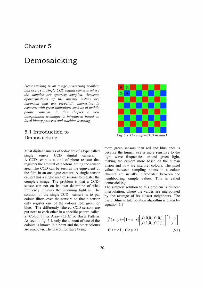
Most digital cameras of today are of a type called single sensor CCD digital camera. A CCD- chip is a kind of photo resistor that registers the amount of photons hitting the sensor area. The CCD can be seen as the equivalent of the film in an analogue camera. A single sensor camera has a single area of sensors to register the complete image. The problem is that a CCD-sensor can not on its own determine of what frequency (colour) the incoming light is. The solution of the single-CCD camera is to put colour filters over the sensors so that a sensor only register one of the colours red, green or blue. The differently filtered CCD-sensors are put next to each other in a specific pattern called a “Colour Filter Array”(CFA) or Bayer Pattern. As seen in fig. 5.1, only the amount of one of the colours is known in a point and the other colours are unknown. The reason for there being

Fig. 5.1 The single-CCD mosaick

more green sensors than red and blue ones is because the human eye is more sensitive to the light wave frequencies around green light, making the camera more based on the human vision and how we interpret colours. The pixel values between sampling points in a colour channel are usually interpolated between the neighbouring sample values. This is called demosaicking. The simplest solution to this problem is bilinear interpolation, where the values are interpolated by the average of its closest neighbours. The basic Bilinear Interpolation algorithm is given by equation 5.1

f x , y ≈[1−x x ][ f 0,0f 1,0

f 0,1f 1,1][1− y

y ]0x1, 0 y1 (5.1)

20

R GG B

in which, f(0,0), f(0,1), f(1,0) and f(1,1) are the four closest values. The demosaick problem is a special case for the bilinear interpolation algorithm. When interpolating the missing green values or the missing red and blue pixel under a blue or red one the interpolation is always on the same distance ( f (0.5, 0.5) ) which correspond to the mean value of the four closest sample points.

This gives equation 5.2 for interpolation for missing green pixel values and the equation 5.3 for missing red and blue pixels that lie over real blue or red pixel values.

The missing pixel values of red and blue over a green pixel value only have two closest neighbours. The missing pixels at these points are interpolated between only the two closest neighbours in bilinear interpolation [12]. Depending on which neighbours are the closest,

Fig. 5.2 False colours

(5.2)

(5.3)

the values are interpolated either in horizontal or vertical direction as in equation 5.4 or 5.5.

f x , y = f x−1, y f x1, y2

(5.4)

f x , y = f x , y−1 f x , y12

(5.5)

The bilinear interpolation has many weaknesses such as loss of sharpness, false colours, and “zipper effect”.

False colours occur around sharp edges and

Fig.. 5.3 Zipper effect

21

f x , y = f x−1, y f x1, y f x , y−1 f x , y14

f x , y = f x−1, y−1 f x−1, y1 f x1, y−1 f x1, y14

appears as differences between colour channels caused by the smearing of the pixel values and seen in fig. 5.2

The zipper effect is a closely related artefact that also can be seen in fig. 5.2. The zipper- effect occurs when every other pixel is of a different intensity around sharp edges and is caused by interpolation over the edge making the interpolated values smear while the true sample values remain. A close-up of this is shown in fig. 5.3.

5.2 LBP Table Demosaicking

One approach to increase the accuracy of interpolations techniques is to use look-up tables with different interpolation techniques depending on the local neighbourhood of the pixel. If the values in the neighbourhood have a certain gradient or the pixel values are of certain amplitude a interpolation technique for this case is used. This introduces some “intelligence” to the system and the results are more likely to be accurate.

There are two different approaches when building a look up table. The first is to predefine the interpolation techniques by using theory like surface formation and determine the interpolation direction by its gradient. Such an interpolation technique is described by Ron Kimmel [9]. The interpolation used for smooth areas is a linear method that uses a weighted sum between the different channels. For high contrast areas the method uses a table of different interpolations for the edge areas of 6 different types in 4-8 different directions.The other way to build an interpolation table is to let the algorithm itself learn how to interpolate the values by machine learning. This type of algorithm uses analysis around the neighbourhood of a training set of images and maps the best fitting interpolation for the neighbourhood in a table. The values in the table are then used in the interpolation of the mosaick into a complete image.

It is in the analysis and mapping of the neighbourhood of image/mosaick that local binary patterns come in to use in the suggested method. In the a simple case a pixels neighbourhood in an RGB-image could be described by its closets pixels within a colour

22

Interpolation

LBPTraining Data Image(s)

Average Value

for each LBP

Mosaick

Scale

-+

Tablelbp0: X1lbp1: X2

.

.

.

Fig 5.4 The training algorithm

channel. If a missing pixel in a mosaick has four closest neighbours within the colour channel of an 8-bit colour image, the neighbourhood could be described by these values and mapped into the table. However this would require a 2(8+8+8+8)

value to represent every case in the neighbourhood and result in a table of the size ~ 4.3 * 109 which would practically be unusable. The Local Binary Code for the same neighbourhood could be represented with a 24 bit mapping code which would only result in a table of size 16.

The suggested method uses data from training data images and stores a value for each Local Binary Pattern in a post in a table where every row corresponds to a Local Binary Pattern. When training a table, the training image is first transformed into a mosaick and interpolated with a linear interpolation technique such as the bilinear interpolation. The difference from the linear interpolation and the original is then calculated and scaled down based on the local variance or contrast. The mean for each LBP code is then stored in the table. The training algorithm is illustrated in fig. 5.4. The linear

interpolation technique used in this first incarnation of the method is the bilinear interpolation.

By doing this, the algorithm “learns” the weaknesses of the initial interpolation based on Local Binary Pattern and then corrects them accordingly when the same interpolation is used on another image.

When demosaicking an image and using the table with the suggested method, an initial linear interpolation is first calculated that is not based on the local binary patterns (in the suggested method bilinear interpolation). The LBP codes for each missing pixel value´s neighbourhood is then calculated. The value stored in the table for each LBP code in the mosaick neighbourhood is then looked up and scaled to fit the variance of the neighbourhoods. The scaled values from the table are finally added to the ones from the initial interpolation. The interpolation algorithm is illustrated in fig. 5.5.

23

Tablelbp0: X1lbp1: X2

.

.

Scale

Interpolation

LBP

Mosaick

+

+

Interpolated Image

Values for LBP

Fig 5.5 The interpolation algorithm

5.3 Scaling Image Values

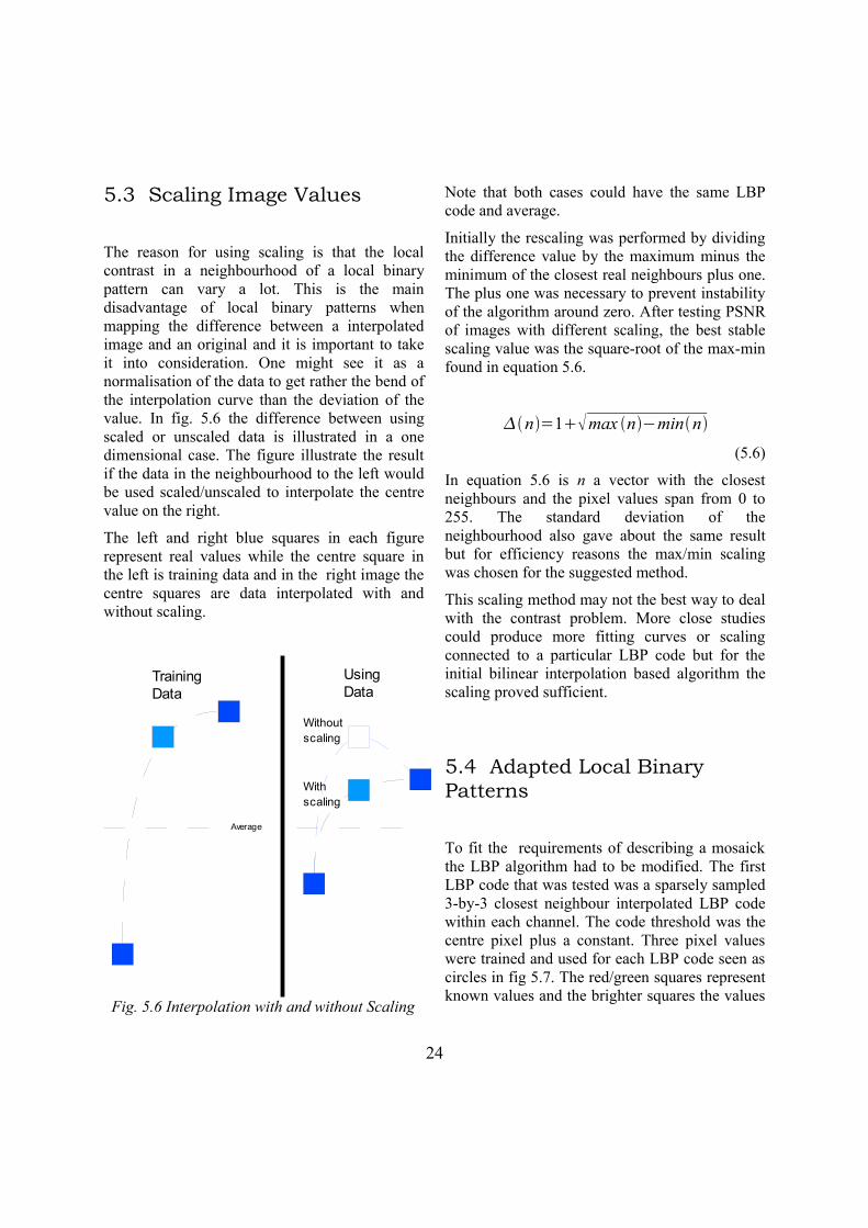
The reason for using scaling is that the local contrast in a neighbourhood of a local binary pattern can vary a lot. This is the main disadvantage of local binary patterns when mapping the difference between a interpolated image and an original and it is important to take it into consideration. One might see it as a normalisation of the data to get rather the bend of the interpolation curve than the deviation of the value. In fig. 5.6 the difference between using scaled or unscaled data is illustrated in a one dimensional case. The figure illustrate the result if the data in the neighbourhood to the left would be used scaled/unscaled to interpolate the centre value on the right.

The left and right blue squares in each figure represent real values while the centre square in the left is training data and in the right image the centre squares are data interpolated with and without scaling.

Fig. 5.6 Interpolation with and without Scaling

Note that both cases could have the same LBP code and average.

Initially the rescaling was performed by dividing the difference value by the maximum minus the minimum of the closest real neighbours plus one. The plus one was necessary to prevent instability of the algorithm around zero. After testing PSNR of images with different scaling, the best stable scaling value was the square-root of the max-min found in equation 5.6.

n=1max n−minn(5.6)

In equation 5.6 is n a vector with the closest neighbours and the pixel values span from 0 to 255. The standard deviation of the neighbourhood also gave about the same result but for efficiency reasons the max/min scaling was chosen for the suggested method.

This scaling method may not the best way to deal with the contrast problem. More close studies could produce more fitting curves or scaling connected to a particular LBP code but for the initial bilinear interpolation based algorithm the scaling proved sufficient.

5.4 Adapted Local Binary Patterns

To fit the requirements of describing a mosaick the LBP algorithm had to be modified. The first LBP code that was tested was a sparsely sampled 3-by-3 closest neighbour interpolated LBP code within each channel. The code threshold was the centre pixel plus a constant. Three pixel values were trained and used for each LBP code seen as circles in fig 5.7. The red/green squares represent known values and the brighter squares the values

24

Average

Without scaling

With scaling

Training Data

Using Data

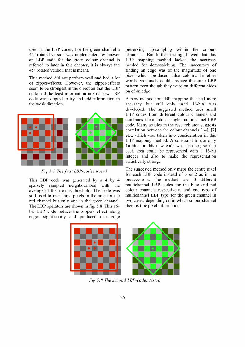
used in the LBP codes. For the green channel a 45° rotated version was implemented. Whenever an LBP code for the green colour channel is referred to later in this chapter, it is always the 45° rotated version that is meant.

This method did not perform well and had a lot of zipper-effects. However, the zipper-effects seem to be strongest in the direction that the LBP code had the least information in so a new LBP code was adopted to try and add information in the weak direction.

This LBP code was generated by a 4 by 4 sparsely sampled neighbourhood with the average of the area as threshold. The code was still used to map three pixels in the area for the red channel but only one in the green channel. The LBP operators are shown in fig. 5.8 This 16-bit LBP code reduce the zipper- effect along edges significantly and produced nice edge

preserving up-sampling within the colour-channels. But further testing showed that this LBP mapping method lacked the accuracy needed for demosaicking. The inaccuracy of finding an edge was of the magnitude of one pixel which produced false colours. In other words two pixels could produce the same LBP pattern even though they were on different sides on of an edge.

A new method for LBP mapping that had more accuracy but still only used 16-bits was developed. The suggested method uses small LBP codes from different colour channels and combines them into a single multichannel-LBP code. Many articles in the research area suggests correlation between the colour channels [14], [7] etc., which was taken into consideration in this LBP mapping method. A constraint to use only 16-bits for this new code was also set, so that each area could be represented with a 16-bit integer and also to make the representation statistically strong.

The suggested method only maps the centre pixel for each LBP code instead of 3 or 2 as in the predecessors. The method uses 3 different multichannel LBP codes for the blue and red colour channels respectively, and one type of multichannel LBP type for the green channel in two cases, depending on in which colour channel there is true pixel information.

25

Fig 5.8 The second LBP-codes tested

Fig 5.7 The first LBP-codes tested

The first type of multichannel LBP code for the red/blue channel is for the case where the pixel value known lie in blue or red channel. If a red pixel is about to be interpolated/mapped and the underlying pixel information is from the blue channel, a 3-by-3 LBP code with the centre as a threshold is calculated for the blue channel. For the remaining channels a 2-by-2 LBP code with the average as threshold for the closest known values in the red and green channels respectively are calculated. The short LBP codes are then fused together to a 16-bit multichannel code according to equation 5.7.

LBP R1=LBP 3x3centre BLBP 2x2average G∗28

LBP2x2 averageR∗212

(5.7)

When a red value in a pixel is going to be interpolated/mapped that has a real green value, two cases occur. The closest two real red values could either lie in horizontal or vertical direction to the value that should be interpolated/mapped. In the suggested method the nine closest green values form a LBP code with the centre as threshold. The six closest red values, with the average as threshold form another LBP code. The two LBP codes are then fused together to form a 12-bit multichannel code as in equation 5.8 or 5.9.

LBP R2=LBP3x3 centreG LBP3x2 averageR∗28

(5.8)

LBP R3=LBP3x3 centreGLBP2x3 averageR∗28

(5.9)

26

Fig. 5.9 The values used in the LBP for the Red Channel

Fig. 5.10 The values used in the LBP for the green channel

These three multichannel LBP codes form the LBP code description for the red colour channel. The same principal is applied when forming the multichannel LBP codes for the blue colour channel.

The multichannel LBP codes for the green colour channel are similar to the first multichannel LBP code of the red channel. The colour channel that has true pixel informations 3-by-3 neighbourhood (red or blue) is threshold with the centre into one LBP code, the green and remaining colour channels 2-by-2 neighbourhoods are respectively thresholded with their averages into two LBP codes. The codes are then fused together to multichannel codes according to equation 5.10 or 5.11.

LBPG1=LBP 3x3centre RLBP2x2 averageG∗28

LBP2x2 average B∗212

(5.10)

LBPG2=LBP 3x3centre BLBP 2x2average G ∗28

LBP 2x2average R∗212

(5.11)

5.5 Results

Some tests have been performed with small datasets. A larger dataset or more similar data could probably increase the results somewhat but the small scale test was sufficient to prove that there could be a future in studying local binary patterns to improve linear demosaicking algorithms.

In the following test a high-resolution sample the lighthouse image was used to interpolate some low-resolution images. The images were used both by Kimmel [4] and Lu/Tan [6] and obtained at [14]. The data is not optimized for the interpolation since it does not seem to be so similar images but it still proved to produce good results. The PSNR results are shown in the table 5.1 below in the order red, green, blue and overall PSNR:

Bilinear Suggested Method

Sails 27.62 32.17 27.96

28.82

31.40 36.11 31.30

32.44

Window 27.58 31.50 27.54

28.52

31.13 35.02 30.84

31.96

Statue 28.91 31.93 28.16

29.39

32.14 35.25 31.72

32.78

Table 5.1

As seen in fig. 5.11, the algorithm also has improved the visual result. The most striking improvement is the gain in sharpness. The algorithm has also removed a lot of zipper- effects which can be seen in the closeups in fig. 5.13. More visual results and the original images can be found in Appendix A.

The goals of the algorithm were to make a self learning algorithm based on local binary patterns

27

that produce both better numerical and visual results than bilinear interpolation. The results show that even under poor conditions the algorithm fulfils these conditions. To further test the algorithm the table trained on the light house image was used to interpolate a colour wedge. The aim of this test was to see if the suggested method has any weakness in interpolation of smooth shifts of colour in where the bilinear interpolation performs well. The resulting image can be seen in fig. 5.12.

The algorithm did not produce any visual artefacts at all in this test. The only difference between bilinear interpolation and the suggested method was of the magnitude of ~1 pixel value which is invisible to the naked eye.

Even though the suggested method has met the goals of this thesis, it does not hold up modern interpolation techniques like the ones described by Kimmel [4] or Lu/Tan [6]. However the

method is still in its infancy and there are many improvements that can be done and tested that is outside the bounds of this thesis. This is discussed in the next section.

28

Fig. 5.11 Bilinear interpolation and the suggested method

Fig. 5.12 Interpolated colour wedge

5.6 Future Research

The first and obvious weakness of the suggested method is the use of the bilinear interpolation in the initial interpolation. A better initial interpolation based on correlation between colour channel as described in [12], [4], [6] could dramatically improve the results. Some initial testing has been done with the interpolation described by Lu and Tan [7] and the standard deviation as a scaling factor. The algorithm was able to increase the PSNR of the high resolution lighthouse image with a value about ~2 dB when the training data was the same image. The LBP code had also been increased 1 bit so that the centre pixel for each code threshold was the average instead of the centre pixel.

But the algorithm was unable to increase the PSNR for any other image than itself as training data even for images similar to each other. This leads to the second weakness in the algorithm which is the scaling. Further research

of the relation of the scaling could be done but I would rather suggest an algorithm that teaches itself the scaling for each LBP code based on a parameter. Such an algorithm could e.g. be based on the standard deviation of the interpolated neighbourhood and use the mean of intervals of the standard deviation to form a parametric curve. Another solution could be to use a parameter based on the values of more than one channel. To use 2 or more extra bits to describe the relation between the colour channels in the LBP code could also be an improvement which is easy to implement.

In addition to these improvements there is the option of post operation steps as a method of reducing artefacts from the interpolation. Lu and Tan [7] suggest a median filter in the colour plane (R-G) and (B-G) around sharp edges to reduce zipper- effect and false colours. Other post operation methods use the gradient to apply a smoothing filter along sharp edges. These methods does not often improve the PSNR result by much but they improve the visual result.

29

Fig. 5.13 Bilinear interpolation and the suggested method

Chapter 6

Conclusions

During this thesis a reconstruction of images from their local binary patterns was presented to prove the preservation of spatial information. Also a new interpolation technique based on local binary patterns and machine learning was developed. The method proved to be better than the bilinear interpolation but did not in its current form reach the high results of modern interpolation techniques.

Reconstructing most of the information of an image from its local binary patterns proved to be possible with the suggested method and the result had good resemblance to the original. The algorithm was also able to reconstruct much information from an image described by uniform patterns. Further development of the reconstruction could probably produce better results, especially for the uniform patterns where the border condition could be implemented as for the ordinary patterns. However, the reconstruction does not have any real use today rather than proving a point.

The demosaicking algorithm presented in this thesis might not meet today´s standard in its current form but has shown some promising results. Due to the time limitation of this thesis there was not enough time to take the algorithm to the next level and challenge today's best algorithms. The suggested method uses the bilinear interpolation and enhances the results from this interpolation but the suggested method is very flexible and can be applied to other interpolation techniques.

Other interesting bi- product results that came out of the research were that the second LBP operator tested in the demosaick section produced good intra channel results. Further research of the phenomena could produce a good self learning up-sampling algorithm. The algorithm could learn what value the missing pixels usually have when an image should be up-sampled by studying a down sampled image. The algorithm could also be applied to a variety of different distortion making it useful in research areas such as super resolution [7], [11].

Even though there are not so many applications that use local binary patterns today, this thesis and the research conducted at the University of Oulu shows that the method is not obsolete but is very useful in many application in computer vision.

30

References

[1] Björn Kruse, Björn Gudmundsson & Dan Antonsson, “PICAP and Relational Neighborhood Pracessing in FIP” pp. 31-46 fr. “Multicomputers and Image Processing Algorithms and Programs”, Academic Press Inc. 1982, ISBN 0-12-564480-9

[2] Benkt Linnander, Lars-Erik Nordell & Björn Kruse, “A Real Time Relational Processor”, The Picture Labrotory, University of Linköping, Linköping, Sweden 1982

[3] A. Jain & G. Healy, “A multiscale representation including opponent color features” IEEE Transactions on Image Processing, No. 7, Vol. 1, January 1998

[4] Ron Kimmel, “Demosaicing: Image Reconstruction from Color CCD Samples” IEEE Transactions on Image Processing, Vol. 8, No.9, September 1999

[5] Khalid Sayood, Introduction to Data Compression, pp. 181-185, Academic Press 2000, ISBN 1-55860-558-4

[6] Wenmiao Lu & Yap-Peng Tan “Color Filter Array Demosaicking: New Method and Performance Measures”, IEEE Transactions on Image Processing, Vol. 12, No. 10, October 2003

[7] David Capel & Andrew Zisserman “Computervision Applied to Super Resolution” IEEE Signal Processing Magazine May 2003

[8] Topi Mäenpää & Matti Pietikäinen, “Texture Analysis with Local Binary Patterns”, Dept. of Electrical and Information Engineering, University of Oulu, Finland, 2004.

[9] Xiaoyi Feng, Abdenour Hadid & Matti Pietikäinen, “A Coarse-to-Fine Classification Scheme for Facial Expression Face Recognition with Local Binary Patterns”, Machine Vision Group, Infotech Oulu, University of Oulu, Finland 2004

[10] M. Heikkilä, M.Pietikäinen, & J. Heikkilä, “A Texture-based Method for Detecting Moving Objects”, Machine Vision Group, Infotech Oulu & Dept. of Electrical and Information Engineering, University of Oulu, Finland 2004

[11] Sina Farsiu, M. Dirk Robinson, Michael Elad & Peyman Milanfar “Fast and Robust Multiframe Super Resolution” IEEE Transactions on Image Proccessing, Vol 13, No 10, October 2004

[12] Henrique S. Malvar, Li-wei He & Ross Cutler “High-Quality Linear Interpolation for Demosaicing of Bayer-Patterned Color Images”, Microsoft Research, USA 2004

[13] Timo Ahonen, Abdenour Hadid & Matti Pietikäinen, “Face Recognition with Local Binary Patterns”, Machine Vision Group, Infotech Oulu, University of Oulu, Finland 2004.

[14] [Online] Available: http://www.cs.technion.ac.il/~ron/Demosaic/

31

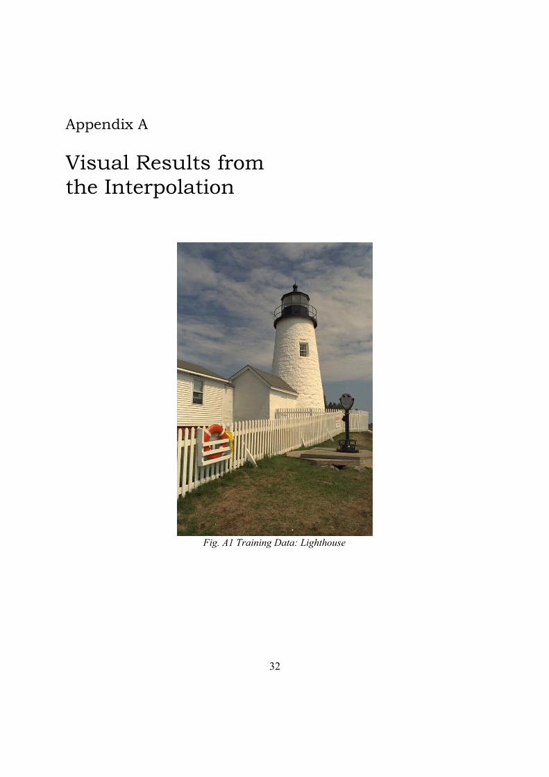
Appendix A

Visual Results from the Interpolation

Fig. A1 Training Data: Lighthouse

32

Fig. A2 Original: Sails Fig. A3 Bilinear interpolation: Sails

Fig. A4 Suggested method: Sails

Fig. A5 Original: Statue Fig. A6 Bilinear interpolation: Statue

Fig. A7 Suggested Method: Statue

33

Fig. A8 Original: Window

Fig. A9 Bilinear: Window

Fig. A10 .Suggested Method: Window

34