study of spin polarisation in simulated high energy pp and

Study of spin polarisation in simulatedhigh energy pp and heavy ion collisions

A project report submitted by

Diptanil RoyRoll No:1411033

to the

School of Physical Sciences

National Institute of Science Education and Research

Bhubaneswar

April 23, 2017

Contents

1 Introduction 3

2 Angular distribution of products in Vector Meson decay 4

3 Thomas Precession 8

4 Scattering, Resonances and Breit Wigner Function 124.1 Resonance . . . . . . . . . . . . . . . . . . . . . . . . . . . . . . . . . 15

5 Polarisation due to Thomas Precession and Asymmetry 16

6 Analysis 216.1 Properties of Φ meson . . . . . . . . . . . . . . . . . . . . . . . . . . 216.2 Event generator - PYTHIA . . . . . . . . . . . . . . . . . . . . . . . 226.3 Analysis techniques . . . . . . . . . . . . . . . . . . . . . . . . . . . . 22

6.3.1 Invariant Mass Reconstruction . . . . . . . . . . . . . . . . . . 226.4 Removal of background : Like-Sign Technique . . . . . . . . . . . . . 23

6.4.1 Fitting . . . . . . . . . . . . . . . . . . . . . . . . . . . . . . . 24

7 Results 277.1 Mass and Width . . . . . . . . . . . . . . . . . . . . . . . . . . . . . 277.2 Angular Distribution and ρ0,0 . . . . . . . . . . . . . . . . . . . . . . 27

8 Inferences and Discussion 29

Appendices 31

A The Code for generating data from PYTHIA 32

B The Code (For Analysis) 35

1

Acknowledgement

It is a strange thing, but when you are dreading something,and would give anything to slow down time, it has adisobliging habit of speeding up.

— J.K.Rowling, Harry Potter and the Goblet of Fire

This quote sums up in entirety how I feel about finishing this work. This project has

been one of my best experiences and has shaped my further interest in research in

physics. As such, this project will be only half done if I do not begin this report by

thanking the people who endured my stupidity at every step, eventually pushing me

over the line.

I start by thanking Sourav Kundu who had initiated me to the lengthy derivations

and made them graspable for me. I thank all the lab members of the Experimental

High Energy Physics Group who sat through my presentations and poured in their

suggestions. I extend my heartfelt gratitude to Ajay Kumar Dash without whose

immense patience, I would still be debugging my code on submission date.

I would also like to reach out to my friends in Physics Batch 14 who have often been

tremendous supports, knowingly or unknowingly. Knowing that your fellow comrades

are as miserable as you is a peace and motivation of another kind, I have realised.

Finally, it is only done when I thank Dr. Bedangadas Mohanty, my guide who has

given me this opportunity to work with this wonderful group and appreciate research

like never before.

2

Chapter 1

Introduction

In physics, you don’t have to go around making trouble foryourself - nature does it for you.

— Frank Wilczek

In this report, we try to understand the orientation of the spin of the constituent quarks

of the produced vector mesons in pp and heavy ion collisions using a simple model. We

argue that this orientation can be due to a relativistic effect called Thomas precession.

In high energy physics, a central collision refers to a head-on collision. In such cases,

the perpendicular distance between the momentum vector of one beam and the center

of mass of the other beam, known as the impact parameter is 0 fm. For non-central

collisions, the impact parameter is non-zero. In case of non-central heavy ion collisions,

it has been shown in [1],[2] that there is a large initial angular momentum which results

in polarisation of the finally produced hadrons. However, the same is not expected of pp

collisions as they are central collisions and hence, there is no initial angular momentum.

A study at STAR collaboration has shown the dependence of the ρ0,0 element on the

transverse momentum for Φ and K∗ produced in pp and Au−Au collisions. For the heavy

ion collision [3], it has been reported in [4] that the ρ0,0 element deviates significantly

from the ‘no-polarisation’ value of 13. However, for the pp collision, ρ0,0 assumes the

value of 13.

In this report, we have analysed a simulated pp collision at√s = 13 TeV generated using

a Monte-Carlo event generator PYTHIA(v. 8186)[5], [6].We have derived an expression

for angular distribution of the produced vector mesons. We have also reproduced the

derivation of polarisation using Thomas precession[4]. Finally, we have shown from the

angular distribution of the produced Φ that the ρ0,0 for Φ is 13.

3

Chapter 2

Angular distribution of productsin Vector Meson decay

“I accept no principles of physics which are not alsoaccepted in mathematics.”

— Rene Descartes

Comments :

• The reaction we are dealing with is the decay of Φ to K+ and K− producedin a symmetric collision. It is a two particle decay and we want to find theangular distribution of the produced particles.

• We will work in the rest frame of Φ .

• Since, we are in the rest frame of Φ , the initial angular momentum ~L is 0. Φ isa spin 1 particle, therefore, total angular momentum ~J = ~L+ ~S = 1.

• Further, since this is a decay, the total angular momentum will be conserved inthe Φ rest frame.

Coordinate System

• We consider a Cartesian coordinate and define the z-axis perpendicular to theplane containing the beam direction vector and the velocity vector of the Φproduced in the collision. (This plane is known as the production plane.)

• Let y-axis be along the velocity vector of Φ . This fixes our coordinate system.

4

• We define θ as the angle the velocity vector of K+ makes with the z-axis and φas its azimuthal angle. We also note that K+ and K− will move opposite toeach other.

• For completely determining the final state, we also need the helicities of thedaughter particles. Let they be λ1 for K+ and λ2 for K− .

j

k

i

~pΦ

z = k × ~pΦ|com

(a)

x

y = ~pΦ|com

z = k × ~pΦ|com

~pK+

θ

~pK−

(b)

Figure 2.1: (a) This system is to determine the production plane and is in the COMframe. (b) In the rest frame of Φ .

Therefore, the final state is given by |f〉 = |θ, φ, λ1, λ2〉.We need the angular distribution of K+ i.e. dN

d cos θdφ. Since, it’s a two particle decay,

N for K+ = N for Φ .dN

d cos θdφ= 〈f |R|f〉 (2.1)

where R = MρM † and M is the decay amplitude of Φ and ρ(K∗) is the densitymatrix of Φ .

dN

d cos θdφ=

⟨θ, φ, λ1, λ2|MρM †|θ, φ, λ1, λ2

⟩(2.2)

=∑λV

∑λV ′

〈θ, φ, λ1, λ2|M |λV 〉〈λV |ρ|λV ′〉⟨λV ′ |M †|θ, φ, λ1, λ2

⟩(2.3)

5

Equation 2.3 has been expanded the RHS in the helicity basis of the Φ .Now, total helicity of the decay product is 0 because they move opposite to eachother(∴ ~s.~p is equal in magnitude and opposite in sign).Since we are looking at two particle decay, |f〉 = |θ, φ, λ1 − λ2〉 = |θ, φ, 0〉. Since, weare in the rest frame of Φ and total angular momentum is conserved, we can writethe final state as |f〉 = |1, 0〉 while being cautious that the θ and φ dependence isstill intact in |f〉.Also, instead of the helicity, we now use the spin as it differs only up to a constantand that can be absorbed in the normalisation constant. Therefore, |λV 〉 = |1,m1〉and |λV ′〉 = |1,m2〉.

dN

d cos θdφ=

∑m1

∑m2

〈1, 0|M |1,m1〉〈1,m1|ρ|1,m2〉⟨1,m2|M †|1, 0

⟩(2.4)

We need to calculate the terms 〈1, 0|M |1,m1〉 and⟨1,m2|M †|1, 0

⟩for which we will

use Wigner-D matrices.Now, in the final state, only the mz component is different than the initial state.Therefore, effectively the operator M acts as a rotation operator which aligns thez-axis along the velocity vector of K+ so that the z-component of spin in the finalstate is 0.

Hence, 〈1, 0|M |1,m1〉 = C ×D1m1,0

(φ, θ,−φ)×√

2J+14π

and⟨1,m2|M †|1, 0

⟩= C∗ ×D∗1m2,0

(φ, θ,−φ)×√

2J+14π

Therefore, Equation 2.4 reduces to

dN

d cos θdφ= |C|2 × 3

4π

∑m1,m2

D1m1,0

(φ, θ,−φ)D∗1m2,0(φ, θ,−φ)ρm1,m2 (2.5)

where ρm1,m2 = 〈1,m1|ρ|1,m2〉 are the elements of the density matrix and J = 1.

Now, we express Dlm,0(α, β, γ) in terms of the spherical harmonics. This is given by

Dlm,0(α, β, γ) =

√4π

2l + 1Y ∗lm(β, α) (2.6)

Therefore, from Equation 2.5, we have 9 terms which we need to calculate usingEquation 2.6. l = 1 for all the 9 terms, ∴ the constant term in Equation 2.6 has a

value of√

4π3

.

6

dN

d cos θdφ= |C|2 ×

∑m1,m2

Y ∗1,m1(θ, φ)Y1,m2(θ, φ)ρm1,m2 (2.7)

Y ∗1,−1Y1,−1 =1

4× 3

2πsin2 θ

Y ∗1,−1Y1,0 =√

21

4× 3

2πsin θ cos θeiφ

Y ∗1,−1Y1,1 = −1

4× 3

2πsin2 θe2iφ

Y ∗1,0Y1,−1 =√

21

4× 3

2πsin θ cos θe−iφ

Y ∗1,0Y1,0 =1

4

3

πcos2 θ

Y ∗1,0Y1,1 = −√

21

4× 3

2πsin θ cos θeiφ

Y ∗1,1Y1,−1 = −1

4

3

2πsin2 θe−2iφ

Y ∗1,1Y1,0 = −√

21

4× 3

2πsin θ cos θe−iφ

Y ∗1,1Y1,1 =1

4× 3

2πsin2 θ

(2.8)

Before putting the values in Equation 2.8 in Equation 2.7, we calculate the φ integralfor all the terms in Equation 2.8.∫ 2π

0

eiφ = 0 ;

∫ 2π

0

e2iφ = 0 (2.9)

Therefore, when we perform the φ integral on Equation 2.7, all the terms containing φbecome 0. Therefore, Equation 2.7 reduces to

dN

d cos θ= |C|2 × 3

8π

[sin2θρ−1,−1 + 2 cos2 θρ0,0 + sin2 θρ1,1

]× 2π

= |C|2 × 3

4

[sin2 θ (ρ−1,−1 + ρ1,1) + 2 cos2 θρ0,0

] (2.10)

Now, from the property of a normalised density matrix, we know that its trace is 1.Therefore, ρ−1,−1 + ρ0,0 + ρ1,1 = 1. Using this in Equation 2.10, we have

dN

d cos θ= |C|2 × 3

4

[sin2 θ (1− ρ0,0) + 2 cos2 θρ0,0

]= |C|2 × 3

4

[1− ρ0,0 + cos2 θ (3ρ0,0 − 1)

]=⇒ dN

d cos θ= N0

[1− ρ0,0 + cos2 θ (3ρ0,0 − 1)

]where N0 is a normalisation constant

(2.11)Equation 2.11 gives the angular distribution of the produced particles as a function ofθ. If there is no polarisation i.e. no preferred direction, ρ0,0 = 1

3. Then, the angular

distribution is a constant (no θ dependence).The next part of the work is to relate the ρ0,0 element to the polarisation of the producedhadrons and compare it to data.

7

Chapter 3

Thomas Precession

“I claim that relativity and the rest of modern physics is notcomplicated. It can be explained very simply. It is onlyunusual or, put another way, it is contrary to commonsense.”

— Edward Teller, Conversation of the Dark Secrets

Thomas Precession is a semi-classical effect originating due to relativistic kinematics.It can simultaneously explain the anomalous Zeeman effect and the fine structuresplitting. The complete explanation for this however comes for Dirac’s relativisticelectron theory which is not explored here.Consider an electron(e−) with a spin angular momentum ~s which can take on quantizedvalues of ±~

2. The magnetic moment of the electron is ~µ = ge

2mc~s where g is the Lande’s

g-factor and is equal to 2. The e− is moving with a velocity ~v in external ~E and ~B.In the rest frame of the e−, the equation of motion is given by(

d~s

dt

)rest frame

= ~µ× ~B′ (3.1)

This is essentially the torque-equivalent on the system.Now, ~B′ = ~B − ~v

c× ~E when we consider up to 1st order in ~a

c. Thus the interaction

energy becomes

∴ U ′ = −~µ.(~B − ~v

c× ~E

)(3.2)

Now, for an electron in an atom, we can estimate the magnitude of the electric forceas the gradient of a radial potential energy V (r). For a one electron system, this is

8

an exact description.

∴ e ~E = −~rr

dV

dr(3.3)

Therefore, the final expression for the spin-interaction energy reduces to

U ′ = − ge

2mc~s. ~B +

g

2m2c2(~s.~L)

1

r

dV

dr(3.4)

Here ~L is the electron’s orbital angular momentum. Now, we have anomalous Zeemaneffect for this case, so g = 2. But experimentally, it has been seen that the resultingspin-orbit interaction term is twice as large.Thomas precession explains this error by accounting for the rotation of the rest frameof the electron coordinate system with respect to the lab frame. Here we will prove anwell-known result which connects the rate of change of any vector in a non-rotatingframe to that in a rotating frame.Consider any vector ~G. Consider two coordinate systems, one fixed (i, j, k) and onerotating (i′, j′, k′) having the same origin.

~G|fixed = ~G|rotating

=⇒ d~G

dt|fixed =

d~G

dt|rotating

=d

dt

(G′1i

′ +G′2j′ +G′3k

′)

=

(dG′1dt

i′ +dG′2dt

j′ +dG′3dt

k′)

+

(G′1di′

dt+G′2

dj′

dt+G′3

dk′

dt

)

=⇒ d~G

dt|fixed =

d~Grotating

dt+

(G′1di′

dt+G′2

dj′

dt+G′3

dk′

dt

)

Now, for infinitesimal rotations, we can write δ ~A = (δθ) n× ~A. Therefore,(d ~Adt

)=(

dθdt

)n× ~A = ~ω × ~A.

di′

dt= ~ω × i′ dj′

dt= ~ω × j′ dk′

dt= ~ω × k′ (3.5)

∴

(d~G

dt

)fixed

=

(d~Grotating

dt

)+ ~ω × ~G (3.6)

9

Using equation 3.6, we have(d~s

dt

)non−rot

=

(d~Grest

dt

)+ ~ω × ~s

=⇒(d~s

dt

)non−rot

= ~s×( ge

2mc~B′ − ωT

)(3.7)

The corresponding energy of interaction is given by

U = U ′ + ~s. ~ωT (3.8)

Consider an electron moving with a velocity ~v(t) with respect to the laboratory frame.The rest frame of the electron is a sequence of co-moving coordinates whose successiveorigins move with the velocity of the electron.Now ~v(t) = c~β at time t and ~v(t+ δt) = c(~β + δ~β).Let x′ be the coordinate of the electron in its rest frame at time t and x′′ at t+ δt.The Lorentz boost matrix is represented by Ab further.

x′ = Ab(~β)x x′′ = Ab(~β + δ~β)x (3.9)

From equation 3.9, we get x′′ = ATx′ where AT = Ab(~β + δ~β)Ab(−~β).

AT =

1 −γ2δβ1 −γδβ2 0

−γ2δβ1 1(γ−1β

)δβ2 0

−γδβ2

(γ−1β

)δβ2 1 0

0 0 0 1

where δβ1, δβ2, δβ3 are components of the vector δ~β and we have used the Lorentztransformation matrices for boosts without rotation.AT essentially represents an infinitesimal Lorentz transformation. We will write themin terms of the generators of Lorentz transform given by ~S and ~K matrices.Using the definitions of ~S and ~K, we have

AT = I −(γ − 1

β2

)(~β × δ~β

).~S −

(γ2δ~β‖ + γδ~β⊥

). ~K (3.10)

Here δ~β‖ and δ~β⊥ are components parallel and perpendicular to ~β respectively.

Up to 1st order in δ~β, equation 3.10 can be written as AT = Ab(∆~β)R(∆~Ω) where

Ab(∆~β) = I −∆~β. ~K and R(∆~Ω) = I −∆~Ω.~S.

10

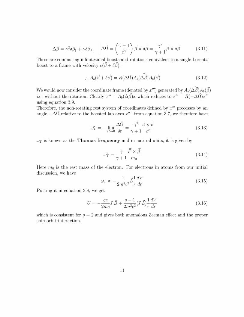
∆~β = γ2δβ‖ + γδβ⊥ ∆~Ω =

(γ − 1

β2

)~β × δ~β =

γ2

γ + 1~β × δ~β (3.11)

These are commuting infinitesimal boosts and rotations equivalent to a single Lorentzboost to a frame with velocity c(~β + δ~β).

∴ Ab(~β + δ~β) = R(∆~Ω)Ab(~

∆~β)Ab(~β) (3.12)

We would now consider the coordinate frame (denoted by x′′′) generated byAb(~

∆~β)Ab(~β)

i.e. without the rotation. Clearly x′′′ = Ab(∆~β)x which reduces to x′′′ = R(−∆~Ω)x′′

using equation 3.9.Therefore, the non-rotating rest system of coordinates defined by x′′′ precesses by anangle −∆~Ω relative to the boosted lab axes x′′. From equation 3.7, we therefore have

~ωT = − limδt→0

∆~Ω

δt=

γ2

γ + 1

~a× ~vc2

(3.13)

ωT is known as the Thomas frequency and in natural units, it is given by

~ωT =γ

γ + 1

~F × ~β

m0

(3.14)

Here m0 is the rest mass of the electron. For electrons in atoms from our initialdiscussion, we have

ωT ≈ −1

2m2c2~L

1

r

dV

dr(3.15)

Putting it in equation 3.8, we get

U = − ge

2mc~s. ~B +

g − 1

2m2c2(~s.~L)

1

r

dV

dr(3.16)

which is consistent for g = 2 and gives both anomalous Zeeman effect and the properspin orbit interaction.

11

Chapter 4

Scattering, Resonances and BreitWigner Function

“In fact, the mere act of opening the box will determine thestate of the cat, although in this case there were threedeterminate states the cat could be in: these being Alive,Dead, and Bloody Furious.”

— Terry Pratchett, Lords and Ladies

We want to look at the scattering of an incident beam off a central target and findthe reaction cross section and the scattering amplitude. We will relate this scatteringamplitude to the polarisation of the produced hadrons.For this, we first consider a plane wave eikz with momentum p = ~k along the z-axis asour incident beam [10]. To make things simple, we assume a central nuclear potentialand express the incident wave as a superposition of incident waves.

ψinc = Aeikz = A

∞∑l=0

il(2l + 1)jl(kr)Pl(cos θ) (4.1)

Here, the jl(kr) are the spherical Bessel functions and are solutions to the radial partof the Schrodinger equation. Pl(cos θ) are the Legendre polynomial and are solutionsto the angular part of the Schrodinger equation. This expansion of the incident waveis called the partial wave equation, with each partial wave corresponding to a specificangular momentum l.

12

When the wave is far from the nucleus, we can expand jl(kr) as

jl(kr) usin(kr − lπ/2)

kr(kr >> l) (4.2)

= ie−i(kr−lπ/2) − ei(kr−lπ/2)

2kr(4.3)

Then the incident wave becomes

ψinc =A

2kr

∞∑l=0

il+1(2l + 1)[e−i(kr−lπ/2) − ei(kr−lπ/2)

]Pl(cos θ) (4.4)

When the scatterer is absent, we can analyse the plane wave as the superposition ofspherically incoming waves involving e−ikr/r and spherically outgoing waves involvingeikr/r.Scattering only affects the outgoing waves by changing its phase or amplitude or both.Change in amplitude is suggestive of fewer particles coming out than going in. Sincethe incident wave represents particles with momentum p = ~k only, for an inelasticscattering, the energy of the particles will change and hence, change in amplitude isexpected.For the lth outgoing partial wave, the changes can be incorporated by introducing acomplex coefficient ηl into the outgoing term (eikr).

ψ =A

2kr

∞∑l=0

il+1(2l + 1)[e−i(kr−lπ/2) − ηlei(kr−lπ/2)

]Pl(cos θ) (4.5)

This wave is a superposition of the incident and the scattered waves ψ = ψinc + ψsc.Therefore,

ψsc =A

2kr

∞∑l=0

il+1(2l + 1)(1− ηl)ei(kr−lπ/2)Pl(cos θ) (4.6)

=A

2k

eikr

r

∞∑l=0

i(2l + 1)(1− ηl)Pl(cos θ) (4.7)

Because we have accounted for partial waves with wavenumber k only, this representsonly elastic scattering. To find the differential cross section, we have

dσ =jscr

2dΩ

jinc(4.8)

13

Now, the scattered current density is given by

jsc =~

2mi

(ψ∗sc

∂ψsc∂r− ψsc

∂ψ∗sc∂r

)(4.9)

= |A|2 ~4mkr2

∣∣∣∣∣∞∑l=0

i(2l + 1)(1− ηl)Pl(cos θ)

∣∣∣∣∣2

(4.10)

Incident current density is given by jinc = ~km|A|2. Therefore, the differential cross

section is

dσ

dΩ=

1

4k2

∣∣∣∣∣∞∑l=0

i(2l + 1)(1− ηl)Pl(cos θ)

∣∣∣∣∣2

(4.11)

Total cross section is given by

σsc =

∫dσ

dΩ=∞∑l=0

λ2

4π(2l + 1)|1− ηl|2 (4.12)

If elastic scattering were the only process that could occur, then |ηl| = 1 and hencewe can write ηl = e2iδl where δl is the phase shift of the lth partial wave. Now,|1− ηl|2 = 4 sin2 δl. Therefore

σsc =∞∑l=0

λ2(2l + 1) sin2 δl (4.13)

For inelastic scattering processes, Eq. 4.13 is not valid as |ηl| < 1. To find thecross section σr due to all such processes, we need to find the rate at which particlesdisappear from a wave with wave number k. This is given by |jin| − |jout| where jinand jout are obtained from the 1st and the 2nd terms of Eq. 4.5 respectively.

|jin| − |jout| =|A|2~4mkr2

∣∣∣∣∣∞∑l=0

il+1(2l + 1)eilπ/2Pl(cos θ)

∣∣∣∣∣2

−∣∣∣∣∣∞∑l=0

il+1(2l + 1)ηle−ilπ/2Pl(cos θ)

∣∣∣∣∣2

(4.14)

σr =∞∑l=0

λ2

4π(2l + 1)(1− |ηl|2) (4.15)

14

Therefore, total cross section involving all processes is

σtot = σsc + σr (4.16)

=∞∑l=0

λ2

2(2l + 1)(1−Re(ηl)) (4.17)

4.1 Resonance

A resonance is the peak located around a certain energy found in differential crosssections of scattering experiments. The resonance will occur when the total crosssection in Eq. 4.17 is maximum. In a single, isolated energy of energy ER and widthΓ, the energy profile will be similar to that for any decaying state of lifetime τ = ~/Γ.Assuming only one partial wave l is important for the resonant state, there will bea scattering resonance where ηl = −1 for δl = π/2. To obtain the shape of theresonance, the cotangent of the phase shift can be expanded in a Taylor series aboutδl = π/2. From this we get

cot δl =E − ER

Γ/2(4.18)

where Γ = 2(∂δl∂E

)−1

E=ERFrom Eq. 4.18, we have

sin δl =Γ/2

[(E − ER)2 + Γ2/4]1/2(4.19)

Therefore, the scattering cross section becomes

σsc =π

k2(2l + 1)

Γ/2

(E − ER)2 + Γ2/4(4.20)

Eq. 4.20 is called the Breit-Wigner formula for the shape of a single, isolated resonancefor elastic scattering.The scattering amplitude is a probability amplitude and the scattering cross sectionis the square of the scattering amplitude.Therefore, from Eq. 4.20, we find that the scattering amplitude A is inverselyproportional to the energy difference between the initial and the final states.

A ∝ 1

∆E(4.21)

We will use this to find out the polarisation asymmetry in a pp-collision due toThomas precession.

15

Chapter 5

Polarisation due to ThomasPrecession and Asymmetry

“Nothing happens until something moves.”

— Albert Einstein

When spin effects are present in a system, we have shown the presence of Thomasprecession which contributes to the difference in energy between the initial and thefinal states. Therefore, the scattering amplitude in its presence is given by

A =1

∆E0 + ~ωT .~s(5.1)

where ∆E0 is the difference in energy among the initial and final states in absence ofspin. If we choose our axis of quantisation to be along the normal to the scatteringplane, polarisation asymmetry is given by

P =|A+|2 − |A−|2|A+|2 + |A−|2

(5.2)

where A+ = 1∆E0+ 1

2ωT

and A− = 1∆E0− 1

2ωT

. Keeping only up to the 1st order terms inωT

2∆E0, we have

P = − ωT∆E0

(5.3)

For hadron formation, one of the main ways is through recombination of a slow anda fast quark. In this process, the resulting hadron is polarised. The semi-classicalpicture which accounts for the polarisation is the Thomas precession produced by

16

the accelerating force that pulls a slow moving quark(qs) [4, 7] or by the deceleratingforce that pulls a fast moving quark(qf) to form a hadron. However, the signs ofpolarisation will be opposite for the two cases. Therefore

P s,f = ∓ ωT∆E0

(5.4)

Before we derive the relevant quantities to describe the spin alignment of vectormeson Φ in pp collisions, we need to make a few assumptions. These are given below:

1. The fast quark (qf ) has a large transverse momentum pf⊥ and zero longitudinal

momentum (pf‖ = 0).

2. The slow quark (qs) moves in the longitudinal direction with momentum ps‖ and

zero transverse momentum (ps⊥ = 0).

3. The rapidity of qs is within the rapidity of hadron’s one (ys = yH) to enhancerecombination probability.

From Eq 3.14, we have ωT =(

γ1+γ

)~F×~βm

where γ is the Lorentz gamma-factor. For

high energy relativistic collisions, we can consider γγ+1≈ 1.

The pulling force ~F is equal to the change in momentum ∆~p of the given quark intime ∆t when the recombination happens. Therefore ~F = ∆~p

∆t. ωT for the given quark

is given by the average over ∆t time interval.

ωs,fT ≈ ∆ps,f

∆tβs,f

(∫∆t

dt sin θs,f/∆t

)(5.5)

= 〈sin θ〉s,f (5.6)

Now, we calculate the change in momenta. For the slow quark qs, we have

∆ps =√

(ps/H‖ − ps‖)2 + (p

s/H⊥ )2 (5.7)

From the definition of rapidity, we have y = 12

ln(E+pzE−pz

)= ln

(E+pzM⊥

). From here, we

can derive that sinh y =p‖M⊥

.

Using assumption 3, we can therefore write that ps‖ = ms⊥ sinh yH =

ms⊥

mH⊥pH‖ = ms

mH⊥pH‖

where ms⊥ = ms as ps⊥ = 0.

We denote the momentum of the slow and the fast quark in the hadron by ps/H andpf/H respectively. So p

s/H‖ represents the longitudinal component of momentum of

the slow quark in the hadron and so on.

17

Therefore,

∆ps =

√(ps/H‖ − ps‖

)2

+ (ps/H⊥ )2 (5.8)

=

√(ps/H‖ − ms

mH⊥pH‖

)2

+ (ps/H⊥ )2 (5.9)

=

√√√√(ps/H‖pH‖− ms

mH⊥

)2 (pH‖

)2

+

(ps/H⊥pH⊥

)2

p2⊥ (5.10)

=

√(x‖ −

ms

mH⊥

)2 (pH‖

)2

+ (x⊥pH⊥ )2 (5.11)

=⇒ ∆ps ≈ x⊥pH⊥ (5.12)

Here x⊥ =ps/H‖pH‖

and x‖ =ps/H⊥pH⊥

. The last step is justified because the major component

of the hadron momentum is the transverse momentum.For the fast quark qf , the change in momentum is similarly given by

∆~pf = ~pf/H‖ − ~pf/H⊥ − ~pf⊥ (5.13)

Now βf initially points along the perpendicular direction. Although qf picks up alongitudinal component following recombination, the dominant component is thetransverse momentum pf⊥. Therefore we get

∆~pf × ~βf = pf/H‖ βf〈sin θ〉f (5.14)

= (1− x‖)pH‖ 〈sin θ〉f (5.15)

where x⊥ + x‖ = 1 as these are momentum fractions. Further, βf is approximated tobe 1.Now, to calculate the value of 〈sin θ〉s, we give a physical argument. The initial

direction of ~βs points along the parallel direction while ∆~psis directed along theperpendicular direction. Therefore, initial angle is π/2. However, post recombination,since the dominant momentum component is the perpendicular one, the angle is 0.Therefore, the average angle is close to π/4 and hence 〈sin θ〉s ≈ 1/sqrt2. Since, wehave characterised this one as a slow quark, instead of our initial argument where weput γ/γ + 1 ≈ 1, we write

ωs = a∆ps

∆t(5.16)

18

where a = γs

1+γsβs〈sin θ〉s is a factor between 0 and 1.

By similar arguments for 〈sin θ〉f , we have 〈sin θ〉f ≈ 1.The change in energy is common to both the accelerating qs and the decelrating qf .

∆E =

[(pf⊥

)2

+(pf‖

)2

+(mf)2]1/2

+[(ps⊥)2 +

(ps‖)2

+ (ms)2]1/2

−[(pH⊥)2

+(pH‖)2

+(mH)2]1/2

(5.17)

Under the assumption that ps⊥ = pf‖ = 0 and (pH‖ )2 << (pH⊥ )2, we have

∆E ≈[(pf⊥

)2

+(mf)2]1/2

+[(ps‖)2

+ (ms)2]1/2

−[(pH⊥)2

+(mH)2]1/2

=

pf⊥

[1 +

(mf )2

2(pf⊥)2

]+ [(ps‖)

2 + (ms)2]1/2 − pH⊥[1 +

(mH)2

2(pH⊥ )2

](5.18)

where the binomial expansion is done with the assumption that the transversemomentum is large compared to the mass for the fast quark and the hadron.Now, for the second term, we have

[(ps‖)2 + (ms)2]1/2 =

[(ms

mH⊥

)2

(pH‖ )2 + (ms)2

]1/2

= ms cosh yH (5.19)

Here we introduce another factor 0 < z < 1 which relates the hadron and qf transversemomenta by pf⊥ = pH⊥/z. This reduces the equation to

∆E =

(1− zz

)pH⊥ +

[z(mf )2 − (mH)2

2pH⊥

]+ms cosh yH

(5.20)

19

Finally, we get the polarisation P s and P f .

P s = −γs

1+γsβsx⊥p

H⊥√

2∆t(1−zz

)pH⊥ +

[z(mf )2−(mH)2

2pH⊥

]+ms cosh yH

(5.21)

P f =

(1−x‖)pH‖∆t(

1−zz

)pH⊥ +

[z(mf )2−(mH)2

2pH⊥

]+ms cosh yH

(5.22)

Given our choice of quantisation axis along the normal to the reaction plane, we canfind the spin density matrices of the slow and the fast quarks. For qs, it is given by

ρqs

=1

2

(1 + Pqs 0

0 1− Pqs

)Similarly for qf , we have

ρqf

=1

2

(1 + Pqf 0

0 1− Pqf

)We assume there is no particular correlation between the two quarks that combineto give a vector meson. Now we can calculate the spin density matrix of the vectormeson by taking a direct product of ρq

sand ρq

fand transforming it to the coupled

basis [8].

ρ =

(1+Pqs )(1+P

qf)

3+PqsPqf0 0

01−PqsPqf

3+PqsPqf0

0 0(1−Pqs )(1−P

qf)

3+PqsPqf

Hence, we have the ρ0,0 element in terms of the polarisation of the two quarks.

ρ0,0 =1− PqsPqf3 + PqsPqf

(5.23)

Using equations 5.22 and 5.21 in equation 5.23, we can find the ρ0,0 element for theproduced hadron. In case of no polarisation in the system, we have ρ0,0 = 1

3. It is

clear from equation 5.23 that presence of polarisation would deviate the ρ0,0 elementfrom 1

3. This will affect the angular distribution as for ρ0,0 = 1

3, dNd cos θ

is a constant,however in presence of polarisation, it will be a function of cos θ as found in equation2.11.

20

Chapter 6

Analysis

6.1 Properties of Φ meson

We have analysed the decay of the Φ vector meson in this report. Some of theimportant properties of Φ particle is listed below [9].

1. Rest mass = 1019.461± 0.019 MeV

2. Quark Content = ss

3. Charge = 0

4. Width = 4.266± 0.031 MeV

5. Lifetime = (1.55± 0.01)× 10−22 s

6. Strangeness = 0, Charmness = 0, Bottomness = 0

7. Total Spin = 1

8. Isospin = 0

9. Major decay channels:

• Φ → K+ + K− (0.489± 0.005) → (We used this in our analysis)

• Φ → K0L + K0

S (0.342± 0.004)

• Φ → ρπ + π+π−π0 (0.1532± 0.0032)

21

6.2 Event generator - PYTHIA

The data for this analysis has been generated using a Monte-Carlo event generatorPYTHIA(v. 8186). The Pythia program can be used to generate high energy events,i.e. sets of outgoing particles produced in the interactions between two incomingparticles. The emphasis is on multiparticle production in collisions between elementaryparticles, particularly e+e−, p+p+ and e−p+ collisions. It contains a library of hardprocesses for initial and nal state parton showers, multiple parton-parton interaction,string fragmentation, beam remnants and particle decays.The different hard processes in PYTHIA can be classified in different ways:[5], [6]

• Number of final particles produced : 2 → 1, 2 → 2, 2 → 3 processes.This aspect is important as higher the number of particles produced, themore complicated the phase space structure is and hence the whole generationprocedure. PYTHIA is optimized for 2→ 1, 2→ 2 processes.

• Physics scenario : Hard QCD processes, Soft QCD processes, Heavy flavourproduction etc.

This data has been generated using all inelastic soft QCD processes(SoftQCD:inelastic= on) for pp collision at

√s = 13 TeV. Soft QCD involves processes where there

is low momentum transfer between the interacting processes. Only the inelasticinteractions have been included as they are dominated by soft QCD. As mentioned inthe discussion on scattering, inelastic interactions result in formation of new particles.Elastic processes do not allow the same.Inelastic processes can be further categorised into nondiffractive, single diffractive,double diffractive and central diffractive processes. The details of these processes arebeyond the scope of this project.

6.3 Analysis techniques

6.3.1 Invariant Mass Reconstruction

Φ decays to K+ and K− with a branching ratio of 0.489. Since the lifetime of Φ isof the order of 10−22 s, we cannot directly detect Φ . However, we can use the fourmomenta of the daughter particles(K+ and K− ) to reconstruct the mass of Φ usingthe invariant mass reconstruction method.For a particle M moving with four momentum P µ = (E, ~p) in the center of massframe, let it decay to particles A and B with four momenta P µ

1 = (E1, ~p1) andP µ

2 = (E2, ~p2) respectively.

22

Now using conservation of four momenta, we can write (E, ~p) = (E1, ~p1) + (E2, ~p2).

∴ E2 − p2 = (E1 + E2)2 − (~p1 + ~p2)2 (6.1)

=⇒ m2M = m2

A +m2B + 2(E1E2 − ~p1. ~p2) (6.2)

We used K+ and K− pairs to generate the invariant mass for reconstruction. Sincewe have taken all the possible pairs of K+ and K− , there will be a combinatorialbackground which we have to reduce using a statistical procedure.

)2Invariant Mass(GeV/c0.96 0.98 1 1.02 1.04 1.06 1.08 1.1 1.12 1.14

Cou

nts

0

1000

2000

3000

4000

5000

Signal

Background

Invariant Mass with combinatorial background

Figure 6.1: Invariant Mass reconstruction along with the combinatorial backgroundfor one cos θ bin

6.4 Removal of background : Like-Sign Technique

The four momenta distribution of K+ and K− are statistically same. However, for apair of K+ , there will never be a peak in the reconstructed invariant mass around themass of Φ . The uncorrelated background in the unlike sign pair sample is estimatedby the number of like-sign pairs within each event. If the numbers of like sign pairs ofK+ and K− are N++ and N−− respectively, the combinatorial background N is givenby their geometric mean multiplied by a factor R. N = 2R

√N++N−−. Therefore,

23

the signal is given by S = N+− − 2R√N++N−−. The factor R accounts for possible

asymmetry in the production of positively and negatively charged particle and(or)asymmetry due to a detector trigger or acceptance bias relative to the particle charge.This technique has the disadvantage that the statistics in the background spectrumis limited to the number of available events. On the other hand, since the numberof unlike-sign pairs and like-sign pairs are calculated within the same event, thenormalization of the determined background to the signal+background spectrum isstraightforward, provided that one knows the R factor with good accuracy.

6.4.1 Fitting

The signal which is obtained after the background reduction is fitted to a Briet-Wignerplus a polynomial function where the Breit-Wigner function is for the resonance peakand the polynomial function is to fit the residual background. Here, we have taken asecond order polynomial of the form ax2 + bx+ c where a, b, c are free parameters.The Breit-Wigner function is taken as

f(E) = YΓ/2

(E − ER)2 + Γ2/4(6.3)

where Y is the yield, Γ is the width of the resonance and ER is the invariant mass atthe resonance peak.Therefore, the total fit function is given by

f(E) = YΓ/2

(E − ER)2 + Γ2/4+ ax2 + bx+ c (6.4)

24

/ ndf 2χ 394.9 / 104

Yield 0.08± 10.39

Width 0.000052± 0.004608

Peak 0.00± 1.02 BgPar1 2.23e+01±3.06e+04 − BgPar2 2.764e+01± 6.689e+04 BgPar3 2.435e+01±3.609e+04 −

)2Invariant Mass(GeV/c1 1.02 1.04 1.06 1.08 1.1

Cou

nts

0

1000

2000

3000

4000

5000 / ndf 2χ 394.9 / 104

Yield 0.08± 10.39

Width 0.000052± 0.004608

Peak 0.00± 1.02 BgPar1 2.23e+01±3.06e+04 − BgPar2 2.764e+01± 6.689e+04 BgPar3 2.435e+01±3.609e+04 −

-1.0 to -0.8θCos

Signal

Breit Wigner + Poly2

Poly2

/ ndf 2χ 612.4 / 104Yield 0.08± 10.23 Width 0.00005± 0.00454 Peak 0.000± 1.019 BgPar1 2.207e+01±3.736e+04 − BgPar2 2.743e+01± 8.102e+04 BgPar3 2.403e+01±4.347e+04 −


Cou

nts

0

1000

2000

3000

4000

5000 / ndf 2χ 612.4 / 104

Yield 0.08± 10.23 Width 0.00005± 0.00454 Peak 0.000± 1.019 BgPar1 2.207e+01±3.736e+04 − BgPar2 2.743e+01± 8.102e+04 BgPar3 2.403e+01±4.347e+04 −

-0.8 to -0.6θCos

Signal


Poly2



Cou

nts

0

1000

2000

3000

4000

5000 / ndf 2χ 448.1 / 104Yield 0.08± 10.17 Width 0.000051± 0.004554 Peak 0.000± 1.019 BgPar1 2.236e+01±3.645e+04 − BgPar2 2.777e+01± 7.945e+04 BgPar3 2.432e+01±4.281e+04 −

-0.6 to -0.4θCos

Signal


Poly2



Cou

nts

0

1000

2000

3000

4000

5000 / ndf 2χ 616.6 / 104


-0.4 to -0.2θCos

Signal


Poly2



Cou

nts

0

1000

2000

3000

4000

5000 / ndf 2χ 629.4 / 104Yield 0.08± 10.41 Width 0.000052± 0.004669 Peak 0.000± 1.019 BgPar1 2.199e+01±3.565e+04 − BgPar2 2.737e+01± 7.795e+04 BgPar3 2.387e+01±4.212e+04 −

-0.2 to 0.0θCos

Signal


Poly2

Figure 6.2: Invariant mass distribution of mK+K− after combinatorial background subtraction fitted witha Briet Wigner + Residual Background function (red line) in different cos θ bins, from cos θ = -1 to cos θ= 0, for pp collisions at

√s = 13 TeV. The contribution from residual background is shown by blue line.

25



Cou

nts

0

1000

2000

3000

4000

5000 / ndf 2χ 385.1 / 104


0.0 to 0.2θCos

Signal


Poly2



Cou

nts

0

1000

2000

3000

4000

5000


0.2 to 0.4θCos

Signal


Poly2



Cou

nts

0

500

1000

1500

2000

2500

3000

3500

4000

4500


0.4 to 0.6θCos

Signal


Poly2



Cou

nts

0

1000

2000

3000

4000

5000 / ndf 2χ 406.3 / 104


0.6 to 0.8θCos

Signal


Poly2



Cou

nts

0

1000

2000

3000

4000

5000 / ndf 2χ 595.7 / 104


0.8 to 1.0θCos

Signal


Poly2

Figure 6.3: Invariant mass distribution of mK+K− after combinatorial background subtraction fitted witha Briet Wigner + Residual Background function (red line) in different cos θ bins, from cos θ = 0 to cos θ= 1, for pp collisions at

√s = 13 TeV. The contribution from residual background is shown by blue line.

26

Chapter 7

Results

7.1 Mass and Width

From our analysis, we can find the the mass of the resonance peak and the width ofthe resonance for each cos θ bin from the fit parameters of the Breit Wigner function.The mass of Φ is found to be almost same to the PDG value while the width isslightly higher.

θCos1− 0.5− 0 0.5 1

)2W

idth

(MeV

/c

4.3

4.4

4.5

4.6

4.7 Width with errors

PDG Width with error

θWidth of the resonance at different cos

(a)

θCos1− 0.5− 0 0.5 1

)2R

eson

ance

pea

k(G

eV/c

1.01944

1.01946

1.01948

1.0195

1.01952

1.01954Resonance peak with errors

PDG Resonance with error

θMass of the resonance at different cos

(b)

Figure 7.1: (a) Width and (b) Mass of the resonance for different cos θ.

7.2 Angular Distribution and ρ0,0

Our main aim is to find the ρ0,0 element from the dNd cos θ

vs cos θ curve. For this, wefind the total number of counts in the invariant mass range 0.9− 1.1 GeV/c2 for eachof the 10 cos θ bins. From this, we will get the dN

d cos θvs cos θ curve.

27

After that, we fit it using the equation 2.11 given by

dN

d cos θ= N0[1− ρ0,0 + cos2 θ(3ρ0,0 − 1)] (7.1)

θCos1− 0.5− 0 0.5 1

θdN

/dC

os

9800

10000

10200

10400

10600

10800

/ ndf 2χ 16.44 / 8 0N 48.05± 1.539e+04

00ρ 0.002383± 0.3272

/ ndf 2χ 16.44 / 8 0N 48.05± 1.539e+04

00ρ 0.002383± 0.3272

θdN/dCos

Theoretical

Angular distribution of decay products

Figure 7.2: The angular distribution of the decay particles as a function of cos θ.

From the fit parameter, we get ρ0,0 = 0.3272± 0.0024.

28

Chapter 8

Inferences and Discussion

“All of physics is either impossible or trivial. It is impossibleuntil you understand it, and then it becomes trivial.”

— Ernest Rutherford

We finally have the mass of the resonance, the width of the resonance and the value

of the density matrix element ρ0,0 from our analysis.

Since our data is produced in a simulation using an event generator, there is no

angular momentum of the initial beams which collide, hence there is no orbital angular

momentum involved in the recombination process. If that is the case, we have already

argued using equation 2.11 that ρ0,0 should be equal to 13. The value we obtained

after analysis agrees with this expectation.

pp collisions are taken as the baseline for heavy ion collisions as many pp collisions

mimic a heavy ion collision, sans a few properties. The spin polarisation is one such

property absent in pp collision as it is essentially central.

The analysis performed here are fairly basic and they can be improved upon by using

better statistical methods, some of which include using pT cuts, rapidity cuts etc. to

filter out spurious data. However, the absence of spin polarisation is clear from the

angular distribution of Φ which was the goal of this project.

29

Bibliography

[1] G. Bunce et al. , Phys. Rev. Lett. 36, lll3 (1976)

[2] Z.-T Liang, X.-N Wang, Physical Review Letters, 94, 102301 (2005).

[3] B.I. Abelev, et al., STAR Collaboration, Phys. Rev. C 77 (2008) 061902

[4] A. Ayala, E. Cuautle, G.H. Corral, J. Magnin and L.M. Montano, Physics LettersB 682 (2010) 408412

[5] T. Sjostrand, S. Mrenna and P. Skands, JHEP05 (2006) 026

[6] T. Sjostrand, S. Mrenna and P. Skands, Comput. Phys. Comm. 178 (2008) 852

[7] T.A. DeGrand, H.I. Miettinen, Phys. Rev. D 24 (1981) 2419.

[8] Z.-T. Liang, X.-N. Wang, Physics Letters B 629 (2005) 2026

[9] C. Patrignani et al. (Particle Data Group), Chin. Phys. C, 40, 100001 (2016)

[10] Kenneth S. Krane, Introductory Nuclear Physics, John Wiley & Sons

30

Appendices

31

Appendix A

The Code for generating data fromPYTHIA

// File: tree.cc

// This is a simple test program.

// Modified by Rene Brun and Axcel Naumann to put the Pythia::event

// into a TTree.

// Copyright (C) 2014 Torbjorn Sjostrand

// Header file to access Pythia 8 program elements.

#include "Pythia8/Pythia.h"

// ROOT, for saving Pythia events as trees in a file.

#include "TTree.h"

#include "TFile.h"

using namespace Pythia8;

int main()

// Create Pythia instance and set it up to generate hard QCD processes

// above pTHat = 20 GeV for pp collisions at 14 TeV.

Pythia pythia;

// Pick new random number seed for each run, based on clock.

pythia.readString("Random:setSeed = on");

pythia.readString("Random:seed = 0");

// setup parametes

const float Ecm = 13000.0; // CM energy in GeV

//pythia.readString("HardQCD:all = on");

//pythia.readString("PhaseSpace:pTHatMin = 20.");

//pythia.readString("Beams:eCM = 14000.");

//pythia.readString("SoftQCD:nonDiffractive = on");

//pythia.readString("SoftQCD:all = on");

32

//pythia.readString("SoftQCD:elastic = on");

//pythia.readString("SoftQCD:singleDiffractive = on");

//pythia.readString("SoftQCD:doubleDiffractive = on");

//pythia.readString("SoftQCD:centralDiffractive = on");

pythia.readString("SoftQCD:inelastic = on");

//pythia.readString("BeamRemnants:reconnectColours=on");

//pythia.readString("BeamRemnants:reconnectRange=5.0");

pythia.init(2212, 2212, Ecm);

//Tune, amount of CR, ... have to be included in config.cmnd

pythia.readFile("config.cmnd");

// pythia.readString("Random:seed");

// pythia.readString("Random:seed = 1245876");

int nEvents = pythia.mode("Main:numberOfEvents");

int nAbort = pythia.mode("Main:timesAllowErrors");

// Set up the ROOT TFile and TTree.

TFile *file = TFile::Open("pytree.root","recreate");

Event *event = &pythia.event;

TTree *T = new TTree("T","ev1 Tree");

T->Branch("event",&event);

// Begin event loop. Generate event; skip if generation aborted.

for (int iEvent = 0; iEvent < 2000000; ++iEvent)

if (!pythia.next()) continue;

// Fill the pythia event into the TTree.

// Warning: the files will rapidly become large if all events

// are saved. In some cases it may be convenient to do some

// processing of events and only save those that appear

// interesting for future analyses.

for (int i = 0; i < pythia.event.size(); ++i)

Int_t ist = pythia.event[i].status();

//select final particles

if ( ist <= 0 )continue;

Float_t eta = pythia.event[i].eta();

Float_t rap = pythia.event[i].y();

Float_t rphi = pythia.event[i].phi();

Float_t pt = pythia.event[i].pT();

Float_t pxx = pythia.event[i].px();

Float_t pyy = pythia.event[i].py();

Float_t pzz = pythia.event[i].pz();

Float_t energy = pythia.event[i].e();

Float_t mass = pythia.event[i].m();

Int_t pidd = pythia.event[i].id();

33

Int_t momid1 = pythia.event[i].mother1();

Int_t momid2 = pythia.event[i].mother2();

Int_t dauid1 = pythia.event[i].daughter1();

Int_t dauid2 = pythia.event[i].daughter2();

//cout<<"I am HERE ================= "<<eta<<"\t"<<pt<<"\t"<<sqrt(pxx*pxx

+ pyy*pyy)<<"\t"<<pidd<<"\t"<<ist<<endl;

//cout<<"I am HERE ==== 2nd Step =============

"<<pidd<<"\t"<<energy<<"\t"<<mass<<"\t"<<rap<<endl;

//cout<<"I am HERE ==== 3rd Step =============

"<<momid1<<"\t"<<momid2<<"\t"<<dauid1<<"\t"<<dauid2<<endl;

//|eta|<1

//if (TMath::Abs(eta)>1)continue;

T->Fill();

// End event loop.

// Statistics on event generation.

pythia.stat();

// Write tree.

T->Print();

T->Write();

T->MakeClass("plot");

delete file;

// Done.

return 0;

34

Appendix B

The Code (For Analysis)

#define TwoMillion_cxx

#include "TwoMillion.h"

#include <TH2.h>

#include <TStyle.h>

#include <TCanvas.h>

void TwoMillion::Loop()

if (fChain == 0) return;

TH2D *KpKm = new TH2D("K+K-","InvariantMassandCosTheta", 200,0.95,1.15,

10, -1, 1);

TH2D *KpKp = new TH2D("K+K+","InvariantMassandCosTheta", 200,0.95,1.15,

10, -1, 1);

TH2D *KmKm = new TH2D("K-K-","InvariantMassandCosTheta", 200,0.95,1.15,

10, -1, 1);

Long64_t nentries = fChain->GetEntriesFast();

Long64_t nbytes = 0, nb = 0;

for (Long64_t jentry=0; jentry<nentries;jentry++)

Long64_t ientry = LoadTree(jentry);

if (ientry < 0) break;

nb = fChain->GetEntry(jentry); nbytes += nb;

Int_t r = 0, s = 0;

Double_t Px1[300], Py1[300], Pz1[300], MassKp[300];

Double_t Px2[300], Py2[300], Pz2[300], MassKm[300];

Int_t Multiplicity = entry_;

for (Int_t a =0; a<Multiplicity; a++) \\Saving the necessary data

Int_t Stat = entry_idSave[a];

if(Stat == 321|| Stat == -321)

if(Stat == 321)

35

Px1[r] = entry_pSave_xx[a];

Py1[r] = entry_pSave_yy[a];

Pz1[r] = entry_pSave_zz[a];

MassKp[r] = entry_mSave[a];

r+=1;

else

Px2[s] = entry_pSave_xx[a];

Py2[s] = entry_pSave_yy[a];

Pz2[s] = entry_pSave_zz[a];

MassKm[s] = entry_mSave[a];

s+=1;

TFile *file = TFile::Open("2mEvents.root");

TH2D* KpKm = (TH2D*)file->Get("K+K-");

TH2D* KpKp = (TH2D*)file->Get("K+K+");

TH2D* KmKm = (TH2D*)file->Get("K-K-");

TH1D* KpKmUnlike[10];

for(int i=0; i< 10; i++)

KpKmUnlike[i] = new TH1D(Form("KpKmUnlike%d",i), Form("KpKmUnlike%d",i),

200, 0.95, 1.15);

TH1D* KpKplike[10];

for(int i=0; i<10; i++)

KpKplike[i] = new TH1D(Form("KpKplike%d",i), Form("KpKplike%d",i), 200,

0.95, 1.15);

TH1D* KmKmlike[10];

for(int i=0; i<10; i++)

KmKmlike[i] = new TH1D(Form("KmKmlike%d",i), Form("KmKmlike%d",i), 200,

0.95, 1.15);

TH1D* bg[10];

for(int i=0; i<10; i++)

36

bg[i] = new TH1D(Form("Bg%d",i), Form("Bg%d",i), 200, 0.95, 1.15);

TH1D* sg[10];

for(int i=0; i<10; i++)

sg[i] = new TH1D("", "", 200, 0.95, 1.15);

TH1D* correctedbg[10];

for(int i=0; i<10; i++)

correctedbg[i] = new TH1D(Form("CorrectedBg%d",i),

Form("CorrectedBg%d",i), 200, 0.95, 1.15);

for(int i=0; i<10; i++)

KpKmUnlike[i] = KpKm->ProjectionX(Form("Unlike%d", i), i+1, i+1);

for(int i=0; i<10; i++)

KpKplike[i] = KpKp->ProjectionX(Form("pplike%d",i), i+1, i+1);

for(int i=0; i<10; i++)

KmKmlike[i] = KmKm->ProjectionX(Form("mmlike%d",i), i+1, i+1);

for(int i = 0; i<10; i++)

for(int b = 1; b<=200; b++)

Double_t nbkg

=2*TMath::Sqrt(KpKplike[i]->GetBinContent(b)*KmKmlike[i]->GetBinContent(b));

bg[i]->SetBinContent(b, nbkg);

Double_t R[10];

for(int i=0; i<10; i++)

R[i] = KpKmUnlike[i]->Integral(150,200, "")/bg[i]->Integral(150, 200, "");

for(int i = 0; i<10; i++)

37

for(int b = 1; b<=200; b++)

Double_t backgr

=2*TMath::Sqrt(KpKplike[i]->GetBinContent(b)*KmKmlike[i]->GetBinContent(b));

correctedbg[i]->SetBinContent(b, backgr);

TCanvas *ComBg = new TCanvas("ComBg","Total",10,10,600,600);

ComBg->cd();

KpKmUnlike[1]->SetMarkerColor(4);

KpKmUnlike[1]->Draw();

correctedbg[1]->SetTitle("Invariant Mass with combinatorial background");

correctedbg[1]->GetXaxis()->SetTitle("Invariant Mass(GeV/c^2)");

correctedbg[1]->GetYaxis()->SetTitle("Counts");

correctedbg[1]->SetMarkerColor(1);

correctedbg[1]->Draw("same");

TLegend *legendn=new TLegend(0.6,0.65,0.88,0.85);

legendn->SetTextFont(72);

legendn->SetTextSize(0.03);

legendn->AddEntry(KpKmUnlike[1],"Signal","l");

legendn->AddEntry(correctedbg[1],"Background","l");

legendn->Draw();

for(int i=0; i<10; i++)

sg[i] -> Add(KpKmUnlike[i], bg[i], 1, -1);

TF1 *f[10];

Double_t Gamma[10];

Double_t Resonance[10];

Double_t dNdCosTheta[10];

Double_t CosThetaBinCenter[] = -0.9, -0.7, -0.5, -0.3, -0.1, 0.1, 0.3,

0.5, 0.7, 0.9;

TCanvas *Canvas[10];

for(int i = 0; i<10; i++)

Canvas[i] = new

TCanvas(Form("Canvas%d",i),Form("Canvas%d",i),10,10,600,600);

Double_t YieldIn[] = 10, 10, -5, -10, 10, 10, 10, 10, 10, 9;

TF1* BgFunc[10];

38

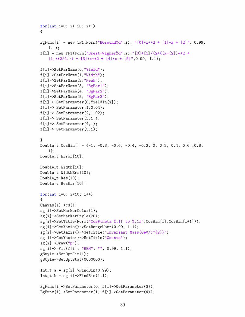
for(int i=0; i< 10; i++)

BgFunc[i] = new TF1(Form("BGround%d",i), "[0]*x**2 + [1]*x + [2]", 0.99,

1.1);

f[i] = new TF1(Form("Breit-Wigner%d",i),"[0]*[1]/(2*((x-[2])**2 +

[1]**2/4.)) + [3]*x**2 + [4]*x + [5]",0.99, 1.1);

f[i]->SetParName(0,"Yield");

f[i]->SetParName(1,"Width");

f[i]->SetParName(2,"Peak");

f[i]->SetParName(3, "BgPar1");



f[i]-> SetParameter(0,YieldIn[i]);

f[i]-> SetParameter(1,0.04);

f[i]-> SetParameter(2,1.02);

f[i]-> SetParameter(3,1 );

f[i]-> SetParameter(4,1);

f[i]-> SetParameter(5,1);

Double_t CosBin[] = -1, -0.8, -0.6, -0.4, -0.2, 0, 0.2, 0.4, 0.6 ,0.8,

1;

Double_t Error[10];

Double_t Width[10];

Double_t WidthErr[10];

Double_t Res[10];

Double_t ResErr[10];

for(int i=0; i<10; i++)

Canvas[i]->cd();

sg[i]->SetMarkerColor(1);

sg[i]->SetMarkerStyle(20);

sg[i]->SetTitle(Form("Cos#theta %.1f to %.1f",CosBin[i],CosBin[i+1]));

sg[i]->GetXaxis()->SetRangeUser(0.99, 1.1);

sg[i]->GetXaxis()->SetTitle("Invariant Mass(GeV/c^2)");

sg[i]->GetYaxis()->SetTitle("Counts");

sg[i]->Draw("p");

sg[i]-> Fit(f[i], "REM", "", 0.99, 1.1);

gStyle->SetOptFit(1);

gStyle->SetOptStat(0000000);

Int_t a = sg[i]->FindBin(0.99);

Int_t b = sg[i]->FindBin(1.1);

BgFunc[i]->SetParameter(0, f[i]->GetParameter(3));


39


BgFunc[i]->SetLineColor(4);

BgFunc[i]->Draw("same");

Width[i] = f[i]->GetParameter(1)*1000;

WidthErr[i] = f[i]->GetParError(1)*1000;

Res[i] = f[i]->GetParameter(2);

ResErr[i] = f[i]->GetParError(2);

TLegend *legend=new TLegend(0.6,0.65,0.88,0.85);

legend->SetTextFont(72);

legend->SetTextSize(0.03);

legend->AddEntry(sg[i],"Signal","lpe");

legend->AddEntry(f[i],"Breit Wigner + Poly2","l");

legend->AddEntry(BgFunc[i],"Poly2","l");

legend->Draw();

dNdCosTheta[i] = f[i]->GetParameter(0)*1000;

Error[i] = TMath::Sqrt(dNdCosTheta[i]);

TF1 *fitf= new TF1("AngularDistro","[0]*(1-[1] + x**2*(3*[1]-1))",-1,1);

fitf->SetParName(0, "N_0");

fitf->SetParName(1, "#rho_00");

fitf->SetParameter(0,100);

fitf->SetParameter(1, 0.33);

TCanvas *C2 = new TCanvas("Angular","",10,10,600,600);

TCanvas *D3 = new TCanvas("New Canvas","",10,10,600,600);

C2->cd();

//

Double_t ErrX[] = 0, 0, 0, 0, 0, 0, 0, 0, 0, 0;

TGraphErrors *Gr = new TGraphErrors(10, CosThetaBinCenter, dNdCosTheta,

ErrX, Error);

Gr->SetMarkerColor(1);

Gr->SetMarkerStyle(20);

Gr->GetXaxis()->SetTitle("Cos#theta");

Gr->GetYaxis()->SetTitle("dN/dCos#theta");

Gr->SetTitle("Angular distribution of decay products");

Gr -> Fit(fitf, "", "", -1, 1);

Gr->Draw();

TLegend *legend2=new TLegend(0.6,0.65,0.88,0.85);

legend2->SetTextFont(72);

legend2->SetTextSize(0.03);

legend2->AddEntry(Gr,"dN/dCos#theta","lpe");

legend2->AddEntry(fitf,"Theoretical","l");

legend2->Draw();

D3->cd();

40

Double_t PDGWid[10];

Double_t PDGWidErr[10];

for(int i = 0; i<10; i++)

PDGWid[i] = 0.004266*1000;

PDGWidErr[i] = 0.000031*1000;

TGraphErrors *Gr1 = new TGraphErrors(10, CosThetaBinCenter, Width, ErrX,

WidthErr);

Gr1->SetMarkerColor(1);

Gr1->SetMarkerStyle(20);

Gr1->GetXaxis()->SetTitle("Cos#theta");

Gr1->GetYaxis()->SetTitle("Width(GeV/c^2)");

Gr1->SetTitle("Width of the resonance at different cos#theta");

Gr1->Draw();

TGraphErrors *GrErr2 = new TGraphErrors(10, CosThetaBinCenter, PDGWid,

ErrX, PDGWidErr);

GrErr2->SetLineColor(2);

GrErr2->Draw("pl same");




legend3->AddEntry(Gr1,"Width with errors","lpe");

legend3->AddEntry(GrErr2, "PDG Width with error", "lpe");

legend3->Draw("p");

TCanvas *D4 = new TCanvas("Resonance","",10,10,600,600);

D4->cd();

Double_t PDGRes[10];

Double_t PDGResErr[10];

for(int i = 0; i<10; i++)

PDGRes[i] = 1.019461;

PDGResErr[i] = 0.000019;

TGraphErrors *Gr2 = new TGraphErrors(10, CosThetaBinCenter, Res, ErrX,

ResErr);

Gr2->SetMarkerColor(1);

Gr2->SetMarkerStyle(20);

Gr2->GetXaxis()->SetTitle("Cos#theta");

Gr2->GetYaxis()->SetTitle("Resonance peak(GeV/c^2)");

Gr2->SetTitle("Value of the resonance at different cos#theta");

Gr2->Draw("apl");

TGraphErrors *GrErr = new TGraphErrors(10, CosThetaBinCenter, PDGRes,

ErrX, PDGResErr);

GrErr->SetLineColor(2);

GrErr->SetMarkerStyle(20);

GrErr->Draw("pl same");

41




legend4->AddEntry(Gr2,"Resonance peak with errors","lpe");

legend4->AddEntry(GrErr, "PDG Resonance with error", "lpe");

legend4->Draw();

TFile *MyFile = new TFile("Plots.root","RECREATE");

MyFile -> cd();

KpKm -> Write();

KpKp -> Write();

KmKm -> Write();

Gr2->Write();

GrErr->Write();

legend4->Write();

for(Int_t i = 0; i<10; i++)

KpKmUnlike[i]->Write();

KpKplike[i] -> Write();

KmKmlike[i] -> Write();

correctedbg[i] -> Write();

sg[i]->SetMarkerColor(1);

sg[i]->SetMarkerSize(1);

sg[i]->SetMarkerStyle(20);

sg[i] -> Write();

BgFunc[i] ->Write();

42

study of spin polarisation in simulated high energy pp and

Documents