study of the inﬂuence of mesh quality on design ... · design optimization procedures : some...

Study of the influence of mesh quality onDesign Optimization procedures : some

examples in FreeFem++

F. HechtLaboratoire Jacques-Louis Lions

Universite Pierre et Marie Curie

Paris, France

with J. Periaux and J. Leskinen

http://www.freefem.org mailto:[email protected]

With the support of ANR (French gov.)

Mars, 14 , 2009, Jyvaskyla 1

http://www.freefem.org

mailto:[email protected]

PLAN

– Introduction Freefem++

– The problem Potientiel/ Navier Stokes

– the mesh constraint

– the mesh adapation

– Optimization algorithms

–

– Conclusion / Future

http://www.freefem.org/


the MDO Problem

The problem is a classical optimization procedure, dealing with a potential

flow around three ellipses where target is just the reconstruction of the

potential values on the three ellipses. Both computation and mesh

generation are done with freefem++ software. Two cases are presented

with mesh adaptation to get a fine result, but the mesh on the ellipses

depend of the solution and of a parameter. So the cost function depends

strongly on the boundary mesh and to show this we try to build mesh with

a constant discretization on the boundary. It is shown on this simple case

how an optimization procedure works in case on constant (prescribed)

mesh on boundary, or do not work otherwise. We will provide an

explanation why and how this result can be generalized.


FreeFem++

FreeFem++ is a software aimed to solve numerically partial differential

equation in IRd, d = 2,3. it is a new version of FreeFem. As its name

indicates, it is a public domain software based on Finite Element Method.

The freefem language allows for a quick specification of any partial

differential system of equations and it can manipulated of data on multiple

meshes.


For who ? For what ?

For R&D, researcher, teacher, professor, student, ...

– To do software prototyping

– To learn or teach Finite Element Method

– To explain variational formulation (weak form)

– To make numerical experiment

– To try new algorithm


The main characteristics of FreeFem++ 2D/(3D) I/III

– Problem description (real or complex) by their variational formulations,

with access to the internal vectors and matrices if needed.

– Multi-variables, multi-equations, bi-dimensional, tri-dimensional , T tri-

dimensional, static or time dependent, linear or nonlinear coupled systems ;

however the user is required to describe the iterative procedures which

reduce the problem to a set of linear problems.

– Easy geometric input by analytic description of boundaries by pieces ; ho-

wever this module is not a CAD system ; for instance when two boundaries

intersect, the user must specify the intersection points.

– Automatic mesh generator, based on the Delaunay-Voronoi algorithm. In-

ner points density is proportional to the density of points on the boundary.


The main characteristics of FreeFem++ 2D/(3D) II/III

– Metric-based anisotropic mesh adaptation in 2D. The metric can be com-

puted automatically from the Hessian of any FreeFem++ function .

– High level user friendly typed input language with an algebra of analytic

and finite element functions.

– Multiple finite element meshes within one application with automatic in-

terpolation of data on different meshes and possible storage of the inter-

polation matrices.

– A large variety of triangular finite elements : contant, linear and qua-

dratic Lagrangian elements , discontinuous P1 (2D) and Raviart-Thomas

elements (2D), elements of a non-scalar type, mini-element, ...(no qua-

drangles).

– Tools to define discontinuous Galerkin/ 2D ? ? formulations via the key-

words : “jump”, “mean”, “intalledges”).


The main characteristics of FreeFem++ 2D/(3D) III/III

– A large variety of linear direct and iterative solvers (LU, Cholesky, Crout,

CG, GMRES, UMFPACK, SuperLU) and eigenvalue and eigenvector sol-

vers.

– Near optimal execution speed (compared with compiled C++ implemen-

tations programmed directly).

– Online graphics with OpenGL/GLUT, generation of ,.txt,.eps,.gnu, mesh

files for further manipulations of input and output data.

– Many examples and tutorials : elliptic, parabolic and hyperbolic problems,

Navier-Stokes flows, elasticity, Fluid structure interactions, Schwarz’s do-

main decomposition method, eigenvalue problem, residual error indicator,

...

– A parallel version using mpi


Last add in 2006.. 2009

– interpolation matrix

– Matrix computation, block matrix, ....

– Variationnel inequality

– dynamic load facility

– New finite element P3, P4, Morley, BernardiRaugel

– Galerkin discontinue P1dc,P2dc,P3dc,P4dc

– New quadrature formular until d◦ 25 in 2D , up d◦ 6 in 3D.

– FFT, special functions j0,j1,jn,y0,y1,yh,erf, erfc, gamma,..

– 3D finites elements : P03d, P13d, P23D

– 3d mesh generation, tetgen, netgen, a layer mesher.

– 3d plot with OpenGL/GLUT library.


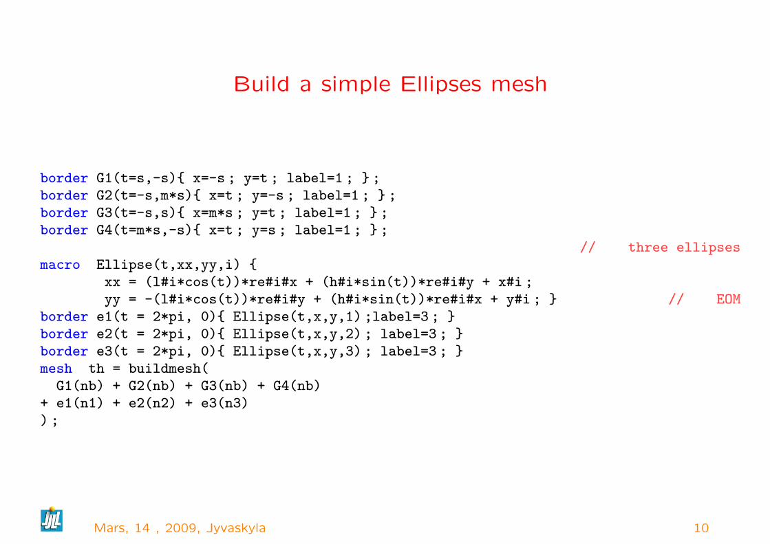
Build a simple Ellipses mesh

border G1(t=s,-s){ x=-s ; y=t ; label=1 ; } ;border G2(t=-s,m*s){ x=t ; y=-s ; label=1 ; } ;border G3(t=-s,s){ x=m*s ; y=t ; label=1 ; } ;border G4(t=m*s,-s){ x=t ; y=s ; label=1 ; } ;

// three ellipsesmacro Ellipse(t,xx,yy,i) {

xx = (l#i*cos(t))*re#i#x + (h#i*sin(t))*re#i#y + x#i ;yy = -(l#i*cos(t))*re#i#y + (h#i*sin(t))*re#i#x + y#i ; } // EOM

border e1(t = 2*pi, 0){ Ellipse(t,x,y,1) ;label=3 ; }border e2(t = 2*pi, 0){ Ellipse(t,x,y,2) ; label=3 ; }border e3(t = 2*pi, 0){ Ellipse(t,x,y,3) ; label=3 ; }mesh th = buildmesh(

G1(nb) + G2(nb) + G3(nb) + G4(nb)+ e1(n1) + e2(n2) + e3(n3)) ;


Solve PDE the problem (a potentiel flow)

// define finite element space

fespace Xh(th,P2) ;

Xh p,q ;

// macros

macro div(u1,u2) (dx(u1)+dy(u2)) //

macro Grad(p) [dx(p),dy(p)] //

problem Potentiel(p,q,solver=CG)= int2d(th)(Grad(p)’*Grad(q)) +

on(1,p=u1infty*x+u2infty*y) ;

// to build the cost ...

real[int] p1(n1),p2(n2),p3(n3) ;

real[int] op1(n1),op2(n2),op3(n3) ;

macro Pboundary(i)

for(int t = 0 ; t < n#i ; t++)

{ real tt = 2.*pi*t/n#i,xx,yy ;

Ellipse(tt,xx,yy,i) ;

p#i(t) = p(xx,yy) ; } // EOM

Pboundary(1) ; Pboundary(2) ; Pboundary(3) ;


Laplace equation in 3d (same coding)

The 3d FreeFem++ code :

mesh3 Th("3dmesh.mesh") ; // load a mesh.

fespace Vh(Th,P13d) ; // define the P1 EF space

Vh u,v ;

macro Grad(u) [dx(u),dy(u),dz(u)] // EOM

solve vlaplace(u,v,solver=CG) =

int3d(Th)( Grad(u)’*Grad(v) ) + int3d(Th) ( 1*v)

+ on(2,u=2) ; // on γ2


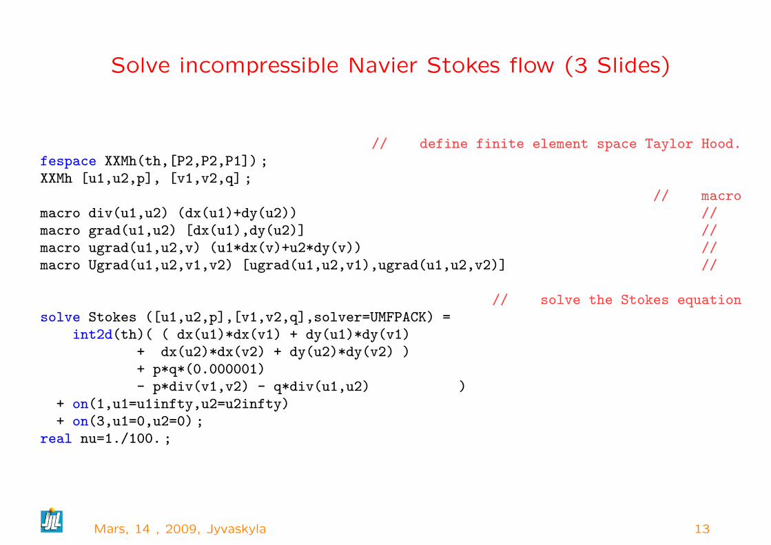
Solve incompressible Navier Stokes flow (3 Slides)

// define finite element space Taylor Hood.fespace XXMh(th,[P2,P2,P1]) ;XXMh [u1,u2,p], [v1,v2,q] ;

// macromacro div(u1,u2) (dx(u1)+dy(u2)) //macro grad(u1,u2) [dx(u1),dy(u2)] //macro ugrad(u1,u2,v) (u1*dx(v)+u2*dy(v)) //macro Ugrad(u1,u2,v1,v2) [ugrad(u1,u2,v1),ugrad(u1,u2,v2)] //

// solve the Stokes equationsolve Stokes ([u1,u2,p],[v1,v2,q],solver=UMFPACK) =

int2d(th)( ( dx(u1)*dx(v1) + dy(u1)*dy(v1)+ dx(u2)*dx(v2) + dy(u2)*dy(v2) )+ p*q*(0.000001)- p*div(v1,v2) - q*div(u1,u2) )

+ on(1,u1=u1infty,u2=u2infty)+ on(3,u1=0,u2=0) ;

real nu=1./100. ;


the tangent PDE

XXMh [up1,up2,pp] ;varf vDNS ([u1,u2,p],[v1,v2,q]) = // Derivative (bilinear part

int2d(th)(+ nu * ( dx(u1)*dx(v1) + dy(u1)*dy(v1)+ dx(u2)*dx(v2) + dy(u2)*dy(v2) )+ p*q*1e-6 + p*dx(v1)+ p*dy(v2)+ dx(u1)*q+ dy(u2)*q+ Ugrad(u1,u2,up1,up2)’*[v1,v2]+ Ugrad(up1,up2,u1,u2)’*[v1,v2] )

+ on(1,2,3,u1=0,u2=0) ;

varf vNS ([u1,u2,p],[v1,v2,q]) = // the RHSint2d(th)(

+ nu * ( dx(up1)*dx(v1) + dy(up1)*dy(v1)+ dx(up2)*dx(v2) + dy(up2)*dy(v2) )+ pp*q*(0.000001)+ pp*dx(v1)+ pp*dy(v2)+ dx(up1)*q+ dy(up2)*q+ Ugrad(up1,up2,up1,up2)’*[v1,v2]

)+ on(1,2,3,u1=0,u2=0)

;


Nolinear Loop, to solve INS with Newton Method on adaptedmesh

for(int rre = 100 ; rre <= 100 ; rre *= 2) // continuation on the reylnods{ re=min(real(rre),100.) ;

th=adaptmesh(th,[u1,u2],p,err=0.1,ratio=1.3,nbvx=100000,hmin=0.03,requirededges=lredges) ;

[u1,u2,p]=[u1,u2,p] ; // after mesh adapt: interpolated old -> new th[up1,up2,pp]=[up1,up2,pp] ;real[int] b(XXMh.ndof),w(XXMh.ndof) ;int kkkk=3 ;for (i=0 ;i<=15 ;i++) // solve steady-state NS using Newton method{ if (i%kkkk==1)

{ kkkk*=2 ; // do mesh adatpationth=adaptmesh(th,[u1,u2],p,err=0.05,ratio=1.3,nbvx=100000,hmin=0.01) ;[u1,u2,p]=[u1,u2,p] ; // resize of array (FE fonction)[up1,up2,pp]=[up1,up2,pp] ;b.resize(XXMh.ndof) ; w.resize(XXMh.ndof) ; }

nu =LL/re ; // set the viscsityup1[]=u1[] ;b = vNS(0,XXMh) ;matrix Ans=vDNS(XXMh,XXMh) ; // build sparse matrixset(Ans,solver=UMFPACK) ;w = Ans^-1*b ; // solve sparse matrixu1[] -= w ;if(w.l2<1e-4) break ; }}


Idea for aniso-mesh with affine Finites Elements

– Equidistribuate the error

– Error on one edge

1

6sup

e∈{a,b,c}supK|t~eH~e|

– Let introduce a metric M (a field on symmetric > 0 matrix, to change

the way to compute a length.


A main IDEA

– The difficulty is to find a tradeoff between the error estimate and the

mesh generation, because this two work are strongly different.

– To do that, we propose way based on a metric M and unit mesh w.r.t M– The metric is a way to control the mesh size.

– remark : The class of the mesh which can be created by the metric, is

very large.


Example of mesh adapted for 2 functions

f1 = (10x3 + y3) + atan2(0.001, (sin(5y)− 2x))

f2 = (10y3 + x3) + atan2(0.01, (sin(5x)− 2y)).

Enter ? for help Enter ? for help Enter ? for help


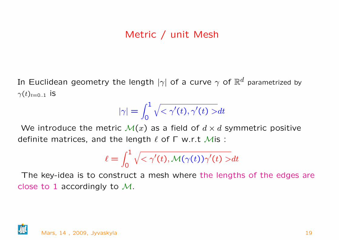
Metric / unit Mesh

In Euclidean geometry the length |γ| of a curve γ of Rd parametrized by

γ(t)t=0..1 is

|γ| =∫ 1

0

√< γ′(t), γ′(t) >dt

We introduce the metric M(x) as a field of d× d symmetric positive

definite matrices, and the length ` of Γ w.r.t Mis :

` =∫ 1

0

√< γ′(t),M(γ(t))γ′(t) >dt

The key-idea is to construct a mesh where the lengths of the edges are

close to 1 accordingly to M.


Remark on the Metric

Let S be a surface , parametrized by

F (u) ∈ R3 with(u) ∈ R2, and let Γ(t) = F (γ(t)), t ∈ [0,1]

be a curve on the surface. The length of the curve Γ is

|Γ| =∫ 1

0

√< Γ′(t),Γ′(t) >dt

|Γ| =∫ 1

0

√< γ′(t), t∂F∂Fγ′(t) >dt

and on a parameteric surface the metric is

M = t∂F∂F


the Metric versus mesh size

at a point P ,

M =

(a bb c

)

M = R(λ1 00 λ2

)R−1

where R = (v1, v2) is the matrix construct with the 2 unit eigenvectors viand λ1, λ2 the 2 eigenvalues.

The mesh size hi in direction vi is given by 1/√λi

λi =1

h2i


Remark on metric :

If the metric is independant of position, then geometry is euclidian. But

the circle in metric become ellipse in classical space.

Infact, the unit ball (ellipse) in a metric given the mesh size in all the

direction, because the size of the edge of mesh is close to 1 the metric.

If the metric is dependant of the position, then you can speak about

Riemmanian geometry, and in this case the sides of triangle are geodesics,

but the case of mesh generation, you want linear edge.


Metrix intersection

The unit ball B(M) in a metrix M plot the maximum mesh size on all the

direction, is a ellipse.

If you two unknows u and v, we just compute the metrix Mv and Mu , find

a metrix Muv call intersection with the biggest ellipse such that :

B(Muv) ⊂ B(Mu) ∩ B(Mv)


2 Direct Problem Demo

Execute ellipse-potentiel/Demo.edp

Execute NSI/NSI-demo.edp


The optimize tools in FreeFem++ to day

– NLGC Non linear Conjugade Gradient

– BFGS the classical BFGS tools

– newuoa a algorithm without derivative from M.J.D. Powell ([email protected])

(add yesterday)

The functionnal

func real J(real[int] & par)

{ real ddd = max( par.linfty-3.,0.) ; // a trick to bound

if (ddd>0) ddd = 100*ddd*ddd ;

real cost ;

include "OnePb.edp"

return cost+ddd ;

}


The code to do optimization process

func real[int] DJ(real[int] & Z)

{

// numerical derivative exercice

real eps=1e-2 ; real[int] par(Z) ;

for(int i=0 ;i<Z.n ;++i)

{ real pari=par[i] ;

par[i]= par[i]-eps ; real c0=J(par) ;

par[i]= par[i]+2*eps ; real c1=J(par) ;

Z[i]= (c1-c0)/(2*eps) ; par[i]= pari ;

}

return Z ;}

real cost1=BFGS(J,DJ,Z,eps=1.e-2,nbiter=15) ;

real cost=newuoa(J,Z,rhobeg=2*Z[0],rhoend=1e-6,npt=N*N+1) ;

Execute ellipse-potentiel/Comp.edp

Execute ellipse-potentiel/Demo-B.edp


Conclusion et future (for freefem++)

It is a useful tool to mixte all equations to teaches Finite Element Method,

to test some nontrivial algorithm and write paper.

– 3D a improvement version

– 3d mesh adaptation

– 3d plot

– add AG optimize tools

– Optimization FreeFem++

– Suite and END.

Thank, for your attention ?


study of the inﬂuence of mesh quality on design ... · design optimization procedures : some...

Documents