Subcontracting Requirements and the Cost of Government

Procurement

Benjamin V Rosa∗

University of Pennsylvania

October 31, 2017

Abstract

Government procurement contracts are frequently subject to policies that specify, as a percentage of

the total project, a subcontracting requirement for the utilization of historically disadvantaged firms. I

study how such subcontracting policies affect procurement auction outcomes using administrative data

from New Mexico’s Disadvantaged Business Enterprise (DBE) Program. My analysis is based on a

procurement auction model with endogenous subcontracting. Theoretically, I show that subcontracting

requirements need not translate into substantially higher procurement costs – even when disadvantaged

firms are relatively more costly. The intuition behind this result is that subcontracting programs require

that prime contractors select their subcontractors from a common pool of disadvantaged firms, which

reduces the private information prime contractors have on their own project-completion costs. As a

result of losing private information, prime contractors strategically reduce their markups in their bids,

and the reduction in markups can be sufficiently high to mitigate the cost increases from using more

costly subcontractors. I estimate an empirical version of the model and find that New Mexico’s past

subcontracting requirements led to only small increases in procurement costs.

∗I thank Mike Abito, Katja Seim, Hanming Fang, Aviv Nevo, and Jorge Balat for their guidance and comments. I would alsolike to thank the participants in the Wharton IO seminar, the AEA Summer Mentoring Pipeline Conference, the InternationalIndustrial Organization Conference, and the Penn empirical micro and theory lunches. I gratefully acknowledge David Coriz ofthe New Mexico Department of Transportation for providing parts of the data.

1

1 Introduction

Public procurement is a sizable part of US government spending. In 2013, public procurement amounted to

26.1 percent of US government spending and just over 10 percent of US GDP.1 The government awards a

portion of that spending to firms that, because of either size or past practices of discrimination, it considers

to be disadvantaged. In 2013, the US federal government awarded 23.4 percent of its procurement spending

to small businesses and 8.61 percent of its procurement spending to small businesses owned and controlled

by ethnic minorities and women.2 To obtain these levels of participation, the US regularly establishes

subcontracting requirements on its federal procurement projects, which specify a percentage of the total

award amount that should be given to preferred firms. For example, if a contract valued at $100, 000 has a

5 percent subcontracting requirement, then $5, 000 of that award must go to preferred firms. In this paper,

I study how these subcontracting policies affect procurement outcomes.

A key feature of subcontracting requirements is that they require prime contractors to complete more of

their projects with subcontractors from a common set of disadvantaged firms. I use a procurement auction

model with endogenous subcontracting to show that this feature can mitigate cost increases associated with

using more costly subcontractors. In the model, prime contractors can complete projects by using a mix of

private resources and subcontractors from a shared pool of disadvantaged firms. I derive a prime contractor’s

bid in this environment as a strategic markup over its project costs, where the markup increases as prime

contractors use more of their own private resources. With subcontracting requirements, prime contractors use

less of their private resources and more disadvantaged subcontractors, which lowers the amount of private

information prime contractors have on their own project costs. Prime contractors therefore reduce their

markups in their bids. The main finding in my paper is that the reduction in markups can be sufficiently

high to leave the cost of procurement virtually unchanged, even if the additional subcontracting increases

project costs.

I estimate an empirical version of the model with administrative highway procurement auction data from

the New Mexico Department of Transportation (NMDOT) in order to evaluate their Disadvantaged Business

Enterprise (DBE) Program. This program relies on subcontracting requirements to increase the representa-

tion of small businesses owned and controlled by socially and economically disadvantaged individuals – who

are primarily ethnic minorities and women – on federal procurement projects. I find that New Mexico’s past

subcontracting requirements are responsible for a 12.7 percent increase in the amount of money awarded to

1See the OECD’s Government at a Glance 2015 report for more information on other countries.2For a full breakdown of small business spending across federal departments, see the FY 2013 Small Business Goaling Report

using the following website: https://www.fpds.gov/fpdsng cms/index.php/en/reports/63-small-business-goaling-report.html.

2

DBE subcontractors yet only increased procurement costs by 0.3 percent. These results suggest that New

Mexico’s subcontracting requirements were not responsible for large increases in procurement costs.

I then use the model to compare subcontracting requirements with two alternative policies geared towards

increasing DBE participation: a quota and a subsidy. I implement the quota by removing prime contractors’

rights to subcontract below the DBE subcontracting requirement, which is currently possible under New

Mexico’s program; I design the subsidy as a payment from the NMDOT to prime contractors proportional to

their DBE utilization. My analysis of these two policies reveals that New Mexico can achieve the same level of

DBE participation at even lower costs of procurement with subsidies relative to subcontracting requirements

and quotas. This outcome is a consequence of subsidies distorting the subcontracting decisions of low project

cost prime contractors less than the other policies. At the level of DBE participation achieved under New

Mexico’s current subcontracting requirements, quotas result in larger amounts of money awarded to DBE

subcontractors relative to the other policies. These results imply that quotas are best for governments seeking

to increase DBE awards, while subsidies are best for governments aiming to reduce procurement costs.

My paper fits into the literature on subcontracting and how it affects firms and auction outcomes. Jeziorski

and Krasnokutskaya (2016) study subcontracting in a dynamic procurement auction, and their model is

closely related to the model in my paper. The main difference between their model and mine is that I study

how different subcontracting policies affect bidding and DBE subcontracting in a static setting. These policies

are frequently used in government procurement and can lead to a variety of different procurement outcomes.

Additionally, their empirical application relies on calibrated parameters, whereas my empirical model allows

me to identify and estimate all of its primitives. Other studies of subcontracting include Marion (2015) who

looks at the effect of horizontal subcontracting on firm bidding strategies, Miller (2014) who explores the effect

of incomplete contracts on subcontracting in public procurement, Nakabayashi and Watanabe (2010) who

use laboratory experiments to investigate subcontract auctions, Branzoli and Decarolis (2015) who study

how different auction formats affect entry and subcontracting choices, Moretti and Valbonesi (2012) who

use Italian data to determine the effects of subcontracting by choice as opposed to subcontracting by law,

and De Silva et al. (2016) who study how subcontracting affects the survival of firms competing for road

construction projects.

There are additional papers within the subcontracting literature that focus on the relationship between

prime contractors and their subcontractors and suppliers. In construction, Gil and Marion (2013) study

how the relationships between prime contractors and their subcontractors shape firm entry and pricing

decisions. Papers in other industries include Kellogg (2011), Masten (1984), and Joskow (1987). My paper

3

abstracts away from many of these more dynamic relationship issues and focuses on a firm’s static incentive

to subcontract with disadvantaged firms.

My paper’s empirical application to DBE subcontracting requirements complements the literature on

subcontracting-based affirmative action policies in government procurement. De Silva et al. (2012) also

study DBE subcontracting requirements and find that DBE subcontracting requirements have negligible

effects on a firm’s cost of completing asphalt projects in Texas. I extend their work by considering how prime

contractors allocate shares of a project to DBE subcontractors and how subcontracting requirements alter

those decisions. Marion (2009, 2017) uses changes in DBE procurement policies to identify the effects of

DBE programs on outcomes such as procurement costs and DBE utilization. My approach differs in that

I use a model to back out a firm’s cost components. The estimated cost components allow me to compare

outcomes across a broad range of counterfactual subcontracting policies. Additional studies on the effects

of these affirmative action policies include De Silva et al. (2015) who find that affirmative action programs

can generate substantial savings for the government and Marion (2011) who studies the effects of affirmative

action programs on DBE utilization in California.

There are a variety of recent studies on similar preference programs in government procurement. Athey

et al. (2013) study set-asides and subsidies for small businesses in US Forest Service timber auctions. They

find that set-asides reduce efficiency and that a subsidy to small businesses is a more effective way to achieve

distributional objectives. My results on quotas and subsidies for disadvantaged subcontractors are similar in

that I find that subsidies are generally less costly for the government relative to quotas. Nakabayashi (2013)

investigates set-asides for small and medium enterprises in Japanese public construction projects and finds

that enough of these smaller enterprises would exit the procurement market in the absence of set-asides to

increase the overall cost of procurement. Empirical papers on bid discounting, which is yet another type of

preference program, include Krasnokutskaya and Seim (2011) and Marion (2007) who study a bid discount

program for small businesses in California and Rosa (2016) who investigates bid discounts for residents in New

Mexico. Hubbard and Paarsch (2009) use numerical simulations to explore how discounts affect equilibrium

bidding.

The remainder of the paper proceeds as follows. Section 2 describes the NMDOT’s procurement process

and DBE Program. Section 3 shows how I model bidding and DBE subcontracting, and section 4 contains

a numerical example from my model. Section 5 shows how I estimate an empirical version of the model,

while section 6 contains my descriptive analysis and estimation results. Section 7 presents my counterfactual

simulations; section 8 concludes.

4

2 New Mexico Highway Procurement

This section describes how the NMDOT awards its construction projects, how the NMDOT’s current DBE

Program operates, and how prime contractors solicit goods and services from DBE subcontractors. The

contents of this section provide the institutional details that guide my modeling choices in later sections.

2.1 Letting

The NMDOT advertises new construction projects four weeks prior to the date of bid opening. As part of

the advertising process, the NMDOT summarizes each project’s main requirements in an Invitation for Bids

(IFB) document. This document contains information on each project’s type of work, location, completion

deadline, DBE subcontracting requirements (if applicable), and licensing requirements. I use the information

in the IFB documents to construct my set of project-level observables.

Interested firms then request the full set of contract documents from the NMDOT and write a proposal

for the completion of each project. In the contract documents, the NMDOT provides firms with an engineer-

estimated cost of the project, which I refer to as the the project’s engineer’s estimate. I include the engineer’s

estimates as an additional variable in my set of project-level observables. The contract proposals contain a

plan for completing the required work, which includes a list of all firms used as subcontractors and a price

for completing each required task. I use data compiled by the NMDOT from the contract documents on the

winning firm’s DBE subcontractors to calculate the share of work allocated to DBE firms.

Firms submit their proposals to the NMDOT through a secure website prior to the date of bid opening.

On the date of bid opening, the NMDOT evaluates all proposals and selects the firm that offers the lowest

total price on all tasks as the winner.3 I model this process as a first-price sealed-bid procurement auction.

2.2 DBE Certification and Subcontracting Requirements

To qualify as a DBE, a firm must show the NMDOT that it is a small business owned and controlled

by socially and economically disadvantaged individuals, who are primarily ethnic minorities and women.

Ownership requires that at least 51 percent of the firm be owned by these disadvantaged individuals, while

control generally requires that disadvantaged individuals have the power to influence the firm’s choices.

The Small Business Administration, which is the federal agency that supports and manages small business

programs, determines whether a firm qualifies as a small business in a particular industry by considering

3The NMDOT can reject the lowest bid if the lowest bidding firm fails to meet DBE subcontracting requirements or qualitystandards. For a more detailed description of the circumstances where the NMDOT will reject a low bid, see the NMDOT’sConsultant Services Procedures Manual available at http://dot.state.nm.us/en/Program Management.html.

5

economic characteristics such as the size of the firm relative to the industry’s average firm size. As part

of the certification process, the NMDOT visits the offices and job sites of DBE applicants to verify their

information. The NMDOT will also routinely check certified DBEs to ensure that they meet the eligibility

requirements. Firms that attempt to participate in the DBE Program based on false information can be

subject to administrative fines and suspension from federal contracting. There are a total of 235 qualified

DBE firms as of April, 2016.4

As a recipient of federal funds, the NMDOT is also required to set an overall state goal for the utilization

of qualified DBE firms on federally assisted construction contracts. The state expresses its DBE utilization

goal as a percentage of total federal funds it awards to DBE firms and has historically been between 7 and

9 percent. If the NMDOT suspects that DBE utilization will fall short of the overall state goal due to either

unanticipated levels of contracts, unforeseen types of contracts, or corrigible deficiencies in the utilization of

DBE firms, the NMDOT can set subcontracting requirements on individual projects, which, similar to the

state goal, requires that prime contractors allocate a pre-specified percentage of the total award amount to

DBE subcontractors.

In setting these requirements on individual contracts, the NMDOT takes a number of factors into con-

sideration. In particular, the NMDOT bases their DBE subcontracting requirements on the type of work

involved on a project, the project’s location, and the availability of DBE subcontractors to perform the type

of work requested on a project. Additionally, the NMDOT will only consider projects with both subcontract-

ing opportunities and estimated costs of more than $300, 000 eligible for DBE subcontracting requirements.

Since those projects are the only ones eligible for subcontracting requirements, much of my empirical and

counterfactual analysis focuses on those larger projects.

Once established, the NMDOT gives prime contractors a number of incentives to meet a project’s sub-

contracting requirement. Although the requirement is not a binding quota, contractors who fall short of the

requirement incur additional costs in the form of showing satisfactory effort to use DBE subcontractors to

the NMDOT as well as having a higher probability of their bid rejected by the NMDOT. Moreover, a prime

contractor that fails to meet a project’s requirement can be fined according to the difference between the

established goal and the achieved level of DBE participation. I model these costs as fines paid by prime

contractors who miss the subcontracting requirement.

4For additional information on the NMDOT’s DBE Program, see the DBE Program Manual available athttp://dot.state.nm.us/en/OEOP.html#c.

6

2.3 Subcontracting with DBE Firms

New Mexico maintains an online DBE system that is accessible to all governments and contractors. Through

this system, prime contractors can find potential DBE subcontractors and request competitive quotes for each

part of a project that requires subcontracting. DBE firms selected as subcontractors have the value of their

services count towards the subcontracting requirement provided that they are performing a commercially

useful function. Given that the DBE system is accessible to all governments and contractors, it is likely that

there are similarities in cost of using DBE subcontractors across firms.

In the model, I represent the cost of using DBE subcontractors with an upward-sloping pricing function

common to all prime contractors. Unfortunately, the New Mexico data does not keep track of the subcon-

tractors used by bidders who do not win, so I cannot directly test whether DBE subcontractor utilization is

common with the data. In other states that have similar DBE systems and that keep public records of DBE

commitments on projects with subcontracting requirements, bidders rarely use different firms in satisfying the

DBE subcontracting requirement. In a sample of lettings from Iowa, for example, 82.4 percent of lettings with

subcontracting requirements and more than one bid had overlap in DBE subcontractors.5 The advantage of

using New Mexico over these states is that I also have data on DBE commitments without subcontracting

requirements. This data variation allows me to separately identify all of my model’s primitives.

In the data, the use of DBE firms as subcontractors is prevalent – even when a project does not have a DBE

subcontracting requirement. In particular, 78 percent of all contracts use at least one DBE subcontractor,

and 62 percent of contracts without a DBE subcontracting requirement use at least one DBE subcontractor.

DBE subcontractors account for a total of 7.1 percent of all contract dollars awarded by the NMDOT.

3 Theoretical Model

In this section, I develop a theoretical model that formalizes the different channels through which DBE

subcontracting requirements affect a prime contractor’s bidding and DBE subcontracting decisions. My

model is closely related to the subcontracting model proposed by Jeziorski and Krasnokutskaya (2016) but

adds a policy that encourages the use of DBE subcontractors.6

5This statistic comes from the Iowa Department of Transportation’s January, 2011 letting, which is available athttps://www.bidx.com/ia/letting?lettingid=11%2F01%2F19. Other lettings from Iowa have a similar pattern.

6Jeziorski and Krasnokutskaya (2016) also include capacity dynamics and entry in their model. In the data, there is no effectof DBE subcontracting requirements on both the set of planholders, which is typically used as a measure of the potential numberof bidders, and the fraction of planholders that eventually become bidders. Moreover, different measures of capacity have littleinfluence on both bidding and DBE subcontractor shares. As a result, the analysis targets bidding and subcontracting strategiesrather than entry and capacity constraints.

7

For each project, prime contractors decide how much work to give DBE subcontractors and how much

to bid. Prime contractors base their decisions on their non-DBE costs of completing the entire project,

which includes work completed in house and by non-DBE subcontractors. My model also incorporates

subcontracting requirements when set by the NMDOT.

3.1 Environment and Objective Function

Formally, N risk-neutral bidders compete against each other for the rights to complete a single, indivisible

highway construction project. Bidders are ex-ante symmetric in that each bidder draws their cost of complet-

ing the entire project without DBE subcontractors, ci, independently from the same distribution, F , with

support on the interval [c, c]. This cost, which I refer to as a bidder’s non-DBE cost, includes work done by

the prime contractor and non-DBE subcontractors. Bidders know the realization of their own non-DBE cost

and the distribution of non-DBE costs prior to submitting bids.

In addition to the standard setup of a first-price sealed-bid procurement auction, all bidders can choose to

subcontract out portions of their projects to DBE firms. That is to say, bidders choose a share of the project,

si ∈ [0, 1], to subcontract to DBE firms, which reduces their portion of the cost of completing the project

from ci to ci (1− si). I model a bidder’s cost of using DBE subcontractors as an increasing, convex, and

twice continuously differentiable pricing function P : [0, 1]→ R+, which is known to all bidders and maps the

share of the project using DBE subcontractors into a price of using DBE subcontractors.7 The cost of using

a DBE subcontracting share of si is then P (si), and I will now refer to this cost as a bidder’s DBE cost. A

limitation of placing this type of structure on the DBE subcontracting market is that it assumes away any type

of private information that a bidder may have on using DBE subcontractors. For example, this assumption

precludes the possibility that contractors may form relationships with certain DBE subcontracting firms to

get discounts on prospective construction projects relative to other contractors. Instead, each bidder has

access to the same DBE subcontracting technology.

Some of the NMDOT’s highway construction projects are subject to DBE subcontracting requirements.

Namely, for every prospective highway construction project, the NMDOT specifies a total share of the project,

s ∈ [0, 1], that is to be completed by DBE subcontractors, and this DBE subcontracting requirement is known

to all bidders prior to any bidding or DBE subcontracting decisions. A choice of s = 0 in this environment

is analogous to not having a subcontracting requirement.

7This pricing function represents the prices received by prime contractors from DBE subcontractors through the quotesolicitation process. Ideally, I would model the DBE subcontracting market separately, and the price would be an endogenousoutcome of that market. However, since the data only contains information on the prices listed by DBE subcontractors, I canonly use prices to infer the cost of using DBE subcontractors. For a discussion of the microfoundations of P , see appendix B.

8

I assume that the NMDOT enforces their subcontracting requirements through fines. These fines represent

any additional costs to bidders who miss the subcontracting requirement, including any actual fines, the

increased probability of bid rejection, and any additional effort required to show the NMDOT satisfactory

effort to use DBE subcontractors. Formally, subcontracting requirements alters a bidder’s optimal choice of

DBE subcontracting and bidding through a fine function ϕ : [0, 1] → R+, which is common knowledge and

maps a bidder’s choice of DBE subcontracting given the DBE subcontracting requirement into a non-negative

value. For technical reasons, I assume that ϕ is non-increasing, convex, and continuously differentiable in all

of its arguments.

In sum, a bidder’s optimization problem is

maxbi,si

(bi − ci (1− si)− P (si)− ϕ (si; s))× Pr (bi < bj∀j ∈ N \ i) . (1)

A strategy in this environment is a 2-tuple that consists of a bid function bi : [c, c] → R+ and a DBE

subcontracting share function si : [c, c] → [0, 1], which, for all levels of s, maps non-DBE costs into bidding

and DBE subcontracting choices. In order to reduce the problem’s complexity, I focus on symmetric Nash

equilibria in bidding and DBE subcontracting; therefore, I drop the i subscript from the bidding and DBE

subcontracting strategies without loss of generality.

The DBE subcontracting market introduces a couple of interesting changes into the competitive bidding

environment. Perhaps the most salient of these changes is that the DBE subcontracting market allows all

bidders to substitute between completing projects with non-DBE resources and with DBE subcontractors.

This substitution benefits the bidders in that increasing the DBE subcontracting share reduces their non-

DBE portion of the cost of completing the contract; however, this substitution is costly in that it requires

bidders to give up a portion of their profits to their DBE subcontractors. Another notable change is that

DBE subcontracting creates a shared component in bidders’ costs of completing the entire project, since all

bidders have equal access to DBE subcontracting.

3.2 DBE Subcontracting Strategies

I begin my analysis of bidding and DBE subcontracting behavior by solving for the optimal DBE subcon-

tracting share given a non-DBE cost realization and a DBE subcontracting requirement. I use the first-order

conditions to characterize an optimal DBE subcontracting share s (ci; s). My analysis of the second-order

conditions is contained in the appendix; see appendix A.1.1. For an interior choice of s (ci; s), the first-order

9

conditions require that

ci = P ′ (si) + ϕ′ (si; s) . (2)

For bidders whose optimal choice is to use no DBE subcontractors, the following condition must hold:

ci < P ′ (0) + ϕ′ (0; s) . (3)

Likewise, bidders whose optimal choice is to subcontract the entire project to DBE firms must have the

following condition hold:

ci > P ′ (1) + ϕ′ (1; s) . (4)

There are a couple of key properties of optimal DBE subcontracting. Similar to Jeziorski and Krasnokut-

skaya (2016), the optimal DBE subcontracting decision does not depend on the probability of winning the

auction. Intuitively, subcontracting only affects a bidder’s objective function through the payoff conditional

on winning and does not directly affect the probability of winning. Bidders therefore do not take the prob-

ability of winning into account when deciding how to use DBE subcontractors. Another characteristic of

optimal DBE subcontracting is that the optimal share does not depend on the bid. In this sense, one can

reinterpret the optimal decisions of a bidder as follows: upon the realization of ci, bidders first determine

how much of the project to subcontract out to DBE firms; then, bidders determine how much to bid given

their optimal choice of si.

Before moving into the bidding strategies, note the effect of DBE subcontracting requirements on DBE

subcontracting decisions. With an interior choice of s (ci; s), assigning a positive DBE subcontracting re-

quirement on a project only affects the DBE subcontractor choice through the marginal fine rather than

the fine’s value. From a policy prospective, bidders are more likely to change their subcontracting behavior

if ϕ changes rapidly in si, implying that policies that impose larger marginal fines for missing the DBE

subcontracting requirement are more effective in changing equilibrium DBE subcontracting shares.

3.3 Bidding Strategies

In addition to selecting a DBE subcontracting share, bidders must also decide on how to bid. To characterize

that decision, I first separate a bidder’s non-DBE cost of completing the project from its total cost of

completing the project, which I will now refer to as its project cost. A bidder’s project cost consists of its

10

non-DBE cost, its DBE costs, and any fines.8 Formally, I define a bidder’s project cost as

φ (ci; s) = ci (1− s (ci; s)) + P (s (ci; s)) + ϕ (s (ci; s) ; s) .

Substituting φ into equation (1) and removing the optimization over si reduces the problem to a first-

price sealed-bid procurement auction, where bidders draw a project cost rather than a non-DBE cost. This

transformed optimization problem together with boundary condition b(φ)

= φ has a unique solution that

is increasing in φ, given arguments from Reny and Zamir (2004), Athey (2001) and Lebrun (2006).9 As a

result, I focus on symmetric bidding strategies that are increasing in φ.

There is a tight relationship between a bidder’s project cost and a bidder’s non-DBE cost. In particular,

observe that

φ′ (ci; s) = (1− s (ci; s)) ≥ 0, (5)

where the above inequality uses the first-order conditions on DBE subcontracting to eliminate the extra

terms in the derivative. Equation (5) demonstrates that the project cost is increasing in ci whenever s (ci; s) ∈

[0, 1) and flat whenever s (ci; s) = 1. Intuitively, bidders with lower non-DBE costs should also have lower

project costs unless their non-DBE costs are high enough that it is optimal to subcontract the entire project

to DBE firms. Furthermore, this relationship implies that the bid function is increasing in ci, except when

s (ci; s) = 1.

Using an envelope theorem argument based on Milgrom and Segal (2002) and equation (5), I derive an

expression for the optimal bid function in terms of non-DBE costs. Proposition 1 presents the bid function

expression, with the details of its derivation contained in appendix A.2.10

Proposition 1. The optimal bid function is

8Recall that one can calculate optimal subcontracting independently of the bid. Therefore, the project cost can be foundprior to bidding and can be substituted in the objective function, obviating the need to optimize over si.

9Observe that φ = P (1) + ϕ (1; s) is the project cost of a bidder that subcontracts the entire project to DBE firms. I derivethis expression from the previous result that the optimal DBE subcontracting share is increasing in ci.

10The NMDOT does not use reservation prices in its procurement auctions, so my model does not include a reservation price.The absence of reservation prices can potentially be problematic, though: when there is only one bidder in an auction, thelack of competition could give rise to unusually high equilibrium bids. To address this problem, I follow Li and Zheng (2009)in assuming that auctions with one bidder face additional competition from the NMDOT in the form of an additional bidderduring the structural estimation and counterfactual policy simulations. This assumption approximates the right of the NMDOTto reject high winning bids. In the data, only 4.6 percent of all auctions have one bidder.

11

b (ci; s) =

∫ cci

(1− s (c; s)) (1− F (c))N−1

dc

(1− F (ci))N−1︸ ︷︷ ︸

Markup

+ ci (1− s (ci; s)) + P (s (ci; s)) + ϕ (s (ci; s) ; s)︸ ︷︷ ︸ .Project Cost

(6)

There are a couple of key features of the bid function. In particular, one can interpret the optimal bid

function as a strategic markup11 over project costs. An increase in DBE subcontracting necessarily reduces

a bidder’s markup and total non-DBE costs. Moreover, the fine function appears as an additive term in the

bid function, meaning that bidders pass fines through to their bids.

3.4 The Role of DBE Subcontracting Requirements

Subcontracting requirements can introduce several interesting changes in equilibrium bidding and DBE sub-

contracting, which come from the features of the equilibrium bid and DBE subcontracting functions. I

summarize those changes in the next proposition and corollaries and provide the proofs of each statement in

appendix A.

Proposition 2. For a given non-DBE cost draw ci, if s (ci; 0) 6= s (ci; s), then s (ci; 0) < s (ci; s).

Proposition 2 says that when the policy can affect a bidder’s DBE subcontracting, subcontracting re-

quirements will increase the share of work given to DBE subcontractors. The idea behind the proof is that

prime contractors want to increase the share of work given to DBE subcontractors to avoid incurring any

fines. Therefore, prime contractors will increase the share of work given to DBE subcontractors when DBE

subcontractors are sufficiently low priced. The next corollary addresses how subcontracting requirements

affect project costs.

Corollary 1. DBE subcontracting requirements weakly raise project costs.

The intuition behind corollary 1 is that, in the absence of DBE subcontracting requirements, bidders

will choose their share of DBE subcontractors to extract the highest possible profits, which in this case is

analogous to minimizing their project costs. As shown in proposition 2, subcontracting requirements can

change DBE subcontracting decisions, and that change leads to higher project costs. The next corollary ties

DBE subcontracting requirements to a bidder’s markup.

11Technically, the markup term contains the bidder’s markup and the markups of all non-DBE subcontractors. I will continueto refer to this term as the markup where this distinction does not cause confusion.

12

Corollary 2. DBE subcontracting requirements weakly lower markups.

The proof of corollary 2 relies on propositions 1 and 2. In particular, the expression for the optimal bid

function in proposition 1 implies that an increase in DBE subcontracting reduces the bidder’s markup, while

proposition 2 shows that DBE subcontracting requirements (weakly) increase total DBE subcontracting.

From those two propositions, it immediately follows that DBE subcontracting requirements weakly lower

markups. Intuitively, subcontracting requirements distort a bidder’s DBE subcontracting decisions towards

completing a project with more DBE subcontractors and less non-DBE resources. Since bidders can only

markup components of their costs that are private and the cost of DBE subcontractors is common, that

distortion leads to a reduction in markups.

4 Numerical Example

In this section, I turn to a numerical example to illustrate the main points of the theory. For this example,

I assume that two prime contractors (N = 2) are competing for a single construction project. I assume that

the prime contractors’ non-DBE costs are distributed uniformly on the interval [0, 1]. For simplicity, I assume

that the pricing functions and the fine function are quadratic and that prime contractors are only fined if

their total share of work going to DBE subcontractors is below the subcontracting requirement:

P (si; τ) =ξs2i

2

ϕ (si; s) =

λ(si−s)2

2 if si < s

0 if si ≥ s,

where ξ and λ are coefficients that control the steepness of the pricing and fine functions respectively. To

keep this example simple, I set ξ = 2; I set the fine coefficient, λ, to 3 so that the fine is sufficiently steep to

visibly change subcontracting behavior. I use a subcontracting requirement of 30 percent (s = 0.3) when it

applies. Figure 1 contains plots of the pricing function and the fine function.

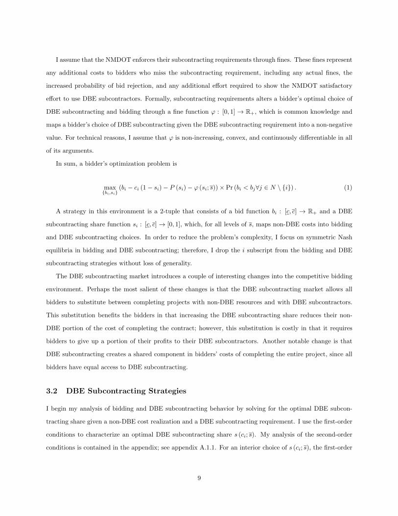
I begin my analysis by first solving for the optimal DBE subcontracting share as a function of non-DBE

costs. To highlight the effects of subcontracting requirements, I perform this calculation twice: once when

there is a requirement and once where there is no requirement. Figure 2 contains plots of these functions.

Subcontracting requirements lead to a couple of interesting changes to DBE subcontracting behavior.

In particular, subcontracting requirements increase the share of work allocated to DBE subcontractors for

13

DBE Share (si)0 0.1 0.2 0.3 0.4 0.5 0.6 0.7 0.8 0.9 1

Price

0

0.1

0.2

0.3

0.4

0.5

0.6

0.7

0.8

0.9

1DBE Pricing Function

DBE Share (si)0 0.1 0.2 0.3 0.4 0.5 0.6

Fin

e

0

0.02

0.04

0.06

0.08

0.1

0.12

0.14Fine Function

Figure 1: DBE Pricing and Fine Functions

prime contractors with lower non-DBE cost draws and leaves shares unchanged for prime contractors with

higher non-DBE cost draws, which is consistent with proposition 2. Intuitively, prime contractors with

lower non-DBE cost draws find it more profitable to use non-DBE resources instead of the relatively more

expensive DBE subcontractors. The fine gives these contractors an extra incentive to increase their DBE

shares, which is why DBE subcontracting is higher for them when there is a requirement. Prime contractors

with higher non-DBE costs are more inclined to use DBE subcontractors to lower their project costs and

may even subcontract above and beyond the requirement. When prime contractors do subcontract above the

requirement, the fine is no longer effective, so there is no change in DBE subcontracting behavior.

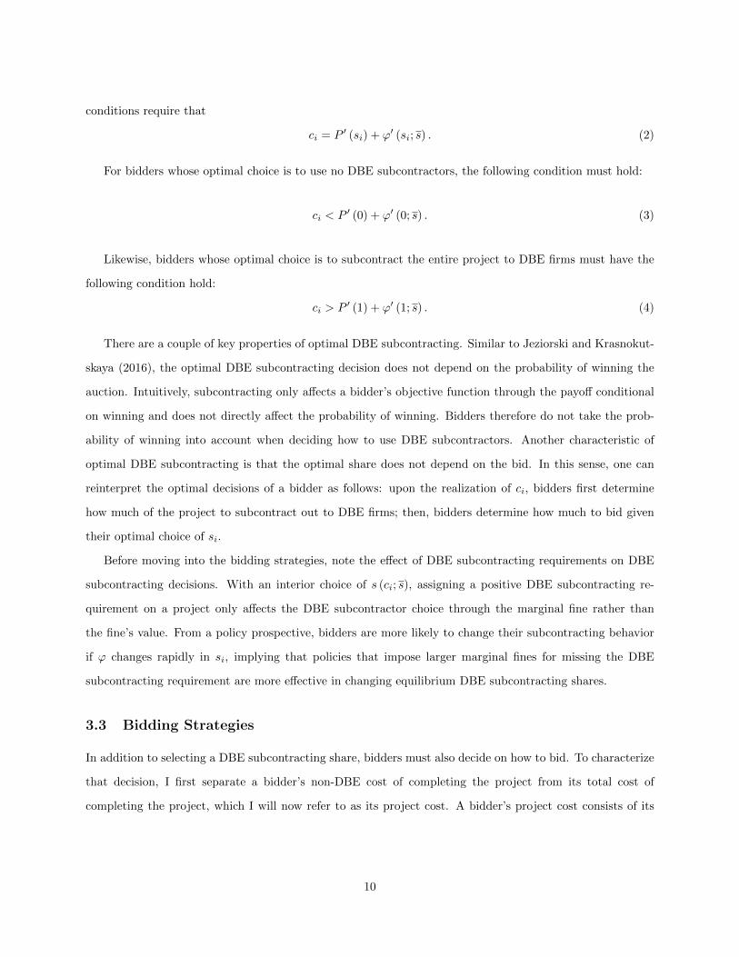
Given the solutions for optimal DBE subcontracting, I next analyze equilibrium bidding with and without

the subcontracting requirement. Specifically, I use equation (6) to obtain a solution for the equilibrium bids

given the uniform assumption on non-DBE costs and the functional forms for the DBE pricing function and

the fine function. I plot these functions in figure 3. A striking feature of the bid functions is that bids are

virtually unchanged with subcontracting requirements relative to without subcontracting requirements, even

when prime contractors draw low non-DBE costs. For this range of non-DBE cost draws, the reduction in

markups is sufficiently high to mitigate the cost of using more DBE subcontractors. Also note that firms

that would subcontract beyond the requirement do not change their bidding behavior, which is why the bid

functions overlap.

Taken together, the simulations demonstrate that subcontracting requirements can increase the share

of work allocated to DBE subcontractors without substantially changing final cost of procurement. The

14

non-DBE cost (ci)0 0.1 0.2 0.3 0.4 0.5 0.6 0.7 0.8 0.9 1

DB

E s

hare

0

0.05

0.1

0.15

0.2

0.25

0.3

0.35

0.4

0.45

0.5

With ReqWithout Req

Figure 2: DBE Share Function

requirement mainly affects prime contractors with low non-DBE costs, causing them to increase their usage

of DBE subcontractors. With sufficiently high markups, increased DBE subcontracting only slightly changes

optimal bidding, implying small changes in procurement costs.

5 Empirical Model and Estimation

Although the theoretical model can account for a number of different ways in which subcontracting require-

ments can affect bidding and DBE subcontracting, it cannot be applied to the New Mexico data without

additional assumptions on the model’s primitives. In this section, I outline those assumptions and provide a

description of the estimation procedure. I end this section by discussing the sources of variation in the data

that identify the empirical model’s parameters.

5.1 Parametric Assumptions

To account for a rich set of observed project characteristics while avoiding the curse of dimensionality, I

estimate a parametric version of the simplified model. I assume that a project, indexed by w, is uniquely

determined by the vector (xw, zw, sw, uw, Nw), where sw is the DBE subcontracting requirement, xw and zw

are potentially overlapping vectors of the remaining project-level observables that affect non-DBE costs and

DBE pricing respectively, uw is a project characteristic unobservable by the econometrician but observable

15

non-DBE cost0 0.1 0.2 0.3 0.4 0.5 0.6 0.7 0.8 0.9 1

Bid

0.4

0.45

0.5

0.55

0.6

0.65

0.7

0.75

0.8

With ReqWithout Req

Figure 3: Bid Function

to the bidders that affects DBE pricing, and Nw is the number of bidders on a project.

I use the project characteristic uw to represent unobserved conditions in the DBE subcontracting market,

such as the availability of DBE firms to act as subcontractors and the concentration of DBE subcontractors in

a particular area. Given that the NMDOT may have extra information on these unobservable characteristics

when establishing a DBE subcontracting requirement, I allow uw to depend on sw. Specifically, I assume

the distribution of uw follows a gamma distribution with a shape parameter of 1 and a scale parameter of

σu = exp (σu0 + σu1DBE req), where DBE req = sw × 100.

I also parameterize the non-DBE cost distribution so that it is consistent with the theory. In particular,

I assume that non-DBE costs follow a truncated log-normal distribution:

ci ∼ T LN(ψ′xw, σ

2c , cw | xw

),

where ψ is a vector of structural parameters that shift the non-DBE cost distribution and cw is the

project-specific upper bound on the non-DBE cost distribution. Given that ci is log normal, its support

is bounded below by 0. I use the variable cw to get the upper limit of integration when solving for the

equilibrium bids in equation (6), and I construct cw by using the highest bid normalized by the engineer’s

estimate in the sample. Specifically, let xw ∈ xw be a project’s engineer’s estimate, and suppose k is the

maximum of the ratio of bids relative to the engineer’s estimate(k = max

biwxw

). Then cw = kxw.12

12Observe that this upper limit is only valid if the observation in which this ratio is maximized has no share of the project

16

I use parametric functional forms for the pricing and fine functions similar to the ones used by Jeziorski

and Krasnokutskaya (2016). In particular, I assume that the DBE pricing function and fine function take

the following functional forms:

P (si) =

(α0 + α1si + α2

si1− si

+ α′3zw + uw

)sixw (7)

ϕ (si; sw) =

γ (si − s)2

x if si < s

0, if si ≥ s. (8)

The hyperbolic term in equation (7) prevents firms from subcontracting entire projects to DBE subcon-

tractors. In the data, no firms select a DBE share of 100%, so I use this functional form to mirror that

empirical fact. The scaling by x in P and ϕ ensures that the problem scales properly, since projects vary

in size; the scaling by si in P ensures that a prime contractor that allocates none of the project to DBE

subcontractors does not have a DBE cost. I use a piecewise functional form in equation (8) so that only

prime contractors who fail to meet the DBE subcontracting requirement will ever be fined. It is important to

note, however, that the parameter values must be constrained for the problem to have desirable properties,

such as an interior maximum, an increasing price function, and a non-increasing fine function for different

parameter guesses. I present these constraints in appendix C.1.

5.2 Estimation

Given a set of structural parameters, my empirical model generates unique solutions for DBE subcontracting

shares and equilibrium bids. The final set of structural parameters are the ones whose predictions are closest

to the outcomes observed in the data. I obtain these parameters with an indirect inference estimator, which

matches the parameters from an auxiliary model estimated with the true data and simulated data.13

I simulate the data in several steps. Given a guess for the structural parameters θ = (ψ, σc, σu, α0, α1, α2,

α3, γ), I first simulate Nw non-DBE costs for each auction. Since bids are increasing in non-DBE costs, I

take the lowest of the Nw non-DBE costs as the non-DBE cost of the winning bidder. Let W denote the

total number of auctions observed in the data and H the total number of simulations. In total, I select

WH non-DBE costs from the∑wNwH simulated non-DBE costs. Next, I calculate the equilibrium DBE

allocated to DBE subcontractors, since the boundary condition on bids is in terms of project costs rather than non-DBE costs.While I do not observe the share of the project allocated to DBE subcontractors for losing bidders, the winning bidder in theauction I use to set k has a DBE share of 0, which makes this approximation plausible.

13Indirect inference was first used by Smith (1993) in a time-series setting and extended by Gourieroux et al. (1993) to a moregeneral form. I use methods from this extended version in estimating the empirical model.

17

subcontracting shares using the first-order conditions on DBE subcontracting in equation (2). To account

for the corner solutions, I take the maximum of 0 and the DBE shares obtained from solving the first-order

conditions for si; the other corner solution is ruled out by the functional form of P (si). With the shares

calculated, I solve for the equilibrium winning bids using equation (6). This step requires an approximation

of the optimal DBE share function, so I use polynomial approximations obtained by fitting a polynomial on

a grid of optimal DBE shares for each auction.

To then implement the indirect inference estimator, I need to select an auxiliary model. In general, the

auxiliary model should be straightforward to estimate and account for the endogenous outcomes. The two

endogenous outcomes are the equilibrium bids and DBE subcontracting shares, so I use a linear ordinary

least squares (OLS) regression of the log-winning bid and a linear OLS regression of the winning bidder’s

DBE subcontracting share as the two components of my auxiliary model. Specifically, if sw is the share of

the project the winning bidder allocates to DBE subcontractors in auction w and bw is the winning bidder’s

bid in auction w, then my auxiliary model for the DBE share and winning bid is

sw =

xw

sw

′

βs + εsw

log(bw) =

xw

sw

′

βb + εbw,

where βs are the parameters of the DBE share regression, βb are the parameters of the winning bid

regression, εsw is the error term on the DBE share regression, and εbw is the error term on the winning bid

regression.

I use a Wald criterion function to match the true data to the simulated data. The indirect inference

structural parameter estimates, θ, are then the solution the following optimization problem:

minθ∈Θ

[βW − βHW (θ)

]′ΩW

[βW − βHW (θ)

],

where βW are the auxiliary model parameters estimated from the data, βHW (θ) are the auxiliary model

parameters estimated from the structural parameters, and ΩW is some positive definite weighting matrix. In

practice, I use the indirect inference estimator’s optimal weight matrix as the weighting matrix, and I use the

estimator’s asymptotic distribution to calculate standard errors. For a detailed explanation of the optimal

weight matrix and standard errors, see appendix C.2.

18

5.3 Parametric Identification

I conclude this section by discussing the variation in the data that identifies the model’s structural parameters.

These parameters are the mean and standard deviation of the non-DBE cost distribution (ψ and σc), the

parameters of the observed components of the DBE pricing function (α0, α1, α2 and α3), the parameters of

the unobserved component of the DBE pricing function (σu0 and σu1), and the fine function parameter (γ).

In the data, I observe projects without subcontracting requirements where prime contractors use no DBE

subcontractors. The bids on these projects allow me to identify the non-DBE cost distribution parame-

ters, since the bid function does not depend on the DBE pricing or fine functions when there are no DBE

subcontractors and no subcontracting requirements.

From there, I can identify the parameters of the observed and unobserved parts of the DBE pricing function

from two types of projects: projects with no subcontracting requirements and projects with subcontracting

requirements where prime contractors exceed the subcontracting requirement. Given the non-DBE cost

distribution parameters, the variation in bids and DBE shares on these projects correspond to changes in

the DBE pricing function. I observe additional variation in bidding and DBE subcontracting between these

two types of projects, and this variation allows me to identify the σu1 parameter – which accounts for the

possibility that the NMDOT assigns subcontracting requirements when it is less costly. Put differently, if

firms tend to use more DBE subcontractors when there is no requirement, then the model would suggest

that the NMDOT uses subcontracting requirements when DBE subcontractors are more costly.

The last parameter that needs to be identified is the fine parameter, γ. Given the non-DBE cost distribu-

tion parameters and DBE pricing function parameters, I identify γ from the bids and DBE shares of prime

contractors who miss the DBE subcontracting requirement. The idea here is that fines only affect bids and

subcontracting when a prime contractor fails to reach a given requirement, so the model attributes differences

in bidding and subcontracting between prime contractors who meet and do not meet the requirement to γ.

6 Empirical Analysis

In this section, I perform the empirical analysis on the procurement data from New Mexico. My analysis

begins with a description of the data and variables. I then present summary statistics and descriptive

regressions to highlight the bidding and DBE subcontracting patterns present in the data. Finally, I provide

the structural parameter estimates and a discussion of the model’s fit.

19

6.1 Data Description and Variables

The data contains federally funded highway construction contracts issued by the NMDOT from 2008 until

2014 for the maintenance and construction of transportation systems. In order to be consistent with the

model, I do not include contracts won by DBE prime contractors.14 I construct the subcontracting portion

of the data from administrative records from New Mexico’s SHARE system. The SHARE data is part of

New Mexico’s state-wide accounting system and tracks all of the transactions between the NMDOT and the

contractors who are ultimately awarded projects using federal aid. This data contains information on the

subcontractors used in each construction project, including each subcontractor’s DBE status and individual

award amount.

I augment the SHARE data with data on contract characteristics. In particular, I include the competition

each winning contractor faces in terms of the actual number of bidders and the number of bidders who request

information about each project, the advertised DBE subcontracting requirement, the type of work necessary

to complete each project, an engineer’s estimated cost of completing each project, and the expected number

of days needed to complete each project in the set of observable project characteristics. I gather this data

from publicly available NMDOT bidding records, which includes the IFB documents the NMDOT uses to

advertise their projects and spreadsheets containing each project’s received bids and eligible bidders.

I define the complete set of variables observed in the full data set as follows. DBE share is the percentage

share of the total project awarded to DBE subcontractors. Engineer’s estimate an engineer’s estimated

cost of a project, which is provided by engineers from the NMDOT. Winning bid is the bid that ultimately

wins the procurement auction. Subprojects are smaller portions of a larger project, which are specified in

the IFB documents and are used as a measure of how easily a contract can use subcontractors.15 Working

days are the number of days a given project is expected to take to complete, and licenses refers to the

number of separate license classifications required to complete the project. Length indicates the length of the

construction project, and DBE req is the level of the DBE subcontracting requirement. Planholders refers

to the number of firms requesting the documents necessary to submit a bid, and federal highway and urban

are indicator variables that take on a value of one if a project is located on a federal highway or an urban

county respectively.

I use additional observables to distinguish a project’s location and the type of work requested for each

project. District is a variable that indicates a project’s administrative district. In New Mexico, there are a

14My model assumes that the prime contractor is not a DBE firm, which is the case for the majority of contracts awardedby the NMDOT. Moreover, prime DBE contractors are not affected by DBE subcontracting requirements, since the primecontractor must perform most of the work.

15See appendix G for an example of subprojects.

20

total of six mutually exclusive districts – each serving a different region of the state. I separate the type of

work requested for each project into six different categories: road work, bridge work, lighting, safety work,

stockpiling, and other. I use the other category as the reference class.

6.2 Summary Statistics

Table 1 presents the summary statistics from the entire sample of NMDOT highway construction contracts.

I divide projects into four categories: projects with subcontracting requirements, projects without subcon-

tracting requirements, projects eligible for subcontracting requirements yet do not have any, and the entire

sample of projects. Recall that New Mexico considers all projects estimated to cost more than $300, 000

eligible for subcontracting requirements.

Table 1: Summary Statistics

With Req. W/o Req. W/o Req. & Eligible Total

Mean Std. Dev. Mean Std. Dev. Mean Std. Dev. Mean Std. Dev.

Eng. Estimate (1000s) 5530.86 6682.41 3817.25 6781.04 4120.84 6975.37 4618.99 6780.67Winning Bid (1000s) 5256.19 6843.40 3438.49 5858.68 3712.46 6019.81 4288.93 6394.94

Bidders 4.64 1.94 4.08 1.93 4.14 1.96 4.34 1.95Subprojects 9.83 5.12 7.21 4.70 7.47 4.78 8.43 5.07

DBE Share (%) 9.15 7.20 4.25 6.29 4.30 5.77 6.54 7.15DBE Req. (%) 4.20 1.91 0.00 0.00 0.00 0.00 1.97 2.47

Share-Req. Gap (%) 4.95 6.91 4.25 6.29 4.30 5.77 4.58 6.59Comply if Req. 0.91 0.29 0.91 0.29

Number of Contracts 182 207 191 389

Table 1 indicates a couple of differences across projects with and without subcontracting requirements.

Projects with subcontracting requirements have, on average, 2.4 more subprojects and are estimated to cost

$1.4 million more than eligible projects without subcontracting requirements. Also, projects with subcon-

tracting requirements allocate 4.9 percentage points more to DBE subcontractors relative to eligible projects

without subcontracting requirements. Despite these differences, projects with subcontracting requirements

tend to attract a similar number of bidders as eligible projects without subcontracting requirements, and

on projects with requirements, many of the prime contractors comply with the requirement – allocating an

average of 5.0 percentage points more than the required amount to DBE subcontractors.

6.3 Descriptive Regressions

In order to explore bidding patterns in the data, I run OLS regressions of the log-winning bids on the covariates

collected from the NMDOT bidding data. Table 2 reports regression coefficients. The main parameter of

21

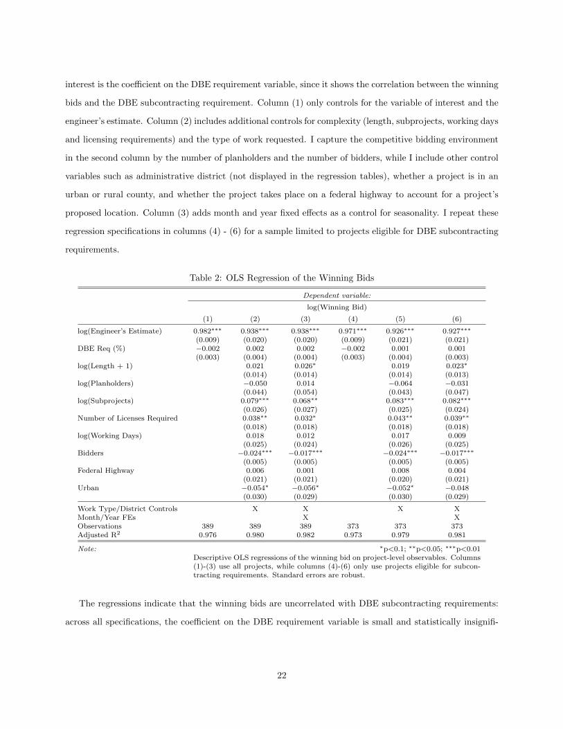
interest is the coefficient on the DBE requirement variable, since it shows the correlation between the winning

bids and the DBE subcontracting requirement. Column (1) only controls for the variable of interest and the

engineer’s estimate. Column (2) includes additional controls for complexity (length, subprojects, working days

and licensing requirements) and the type of work requested. I capture the competitive bidding environment

in the second column by the number of planholders and the number of bidders, while I include other control

variables such as administrative district (not displayed in the regression tables), whether a project is in an

urban or rural county, and whether the project takes place on a federal highway to account for a project’s

proposed location. Column (3) adds month and year fixed effects as a control for seasonality. I repeat these

regression specifications in columns (4) - (6) for a sample limited to projects eligible for DBE subcontracting

requirements.

Table 2: OLS Regression of the Winning Bids

Dependent variable:

log(Winning Bid)

(1) (2) (3) (4) (5) (6)

log(Engineer’s Estimate) 0.982∗∗∗ 0.938∗∗∗ 0.938∗∗∗ 0.971∗∗∗ 0.926∗∗∗ 0.927∗∗∗

(0.009) (0.020) (0.020) (0.009) (0.021) (0.021)DBE Req (%) −0.002 0.002 0.002 −0.002 0.001 0.001

(0.003) (0.004) (0.004) (0.003) (0.004) (0.003)log(Length + 1) 0.021 0.026∗ 0.019 0.023∗

(0.014) (0.014) (0.014) (0.013)log(Planholders) −0.050 0.014 −0.064 −0.031

(0.044) (0.054) (0.043) (0.047)log(Subprojects) 0.079∗∗∗ 0.068∗∗ 0.083∗∗∗ 0.082∗∗∗

(0.026) (0.027) (0.025) (0.024)Number of Licenses Required 0.038∗∗ 0.032∗ 0.043∗∗ 0.039∗∗

(0.018) (0.018) (0.018) (0.018)log(Working Days) 0.018 0.012 0.017 0.009

(0.025) (0.024) (0.026) (0.025)Bidders −0.024∗∗∗ −0.017∗∗∗ −0.024∗∗∗ −0.017∗∗∗

(0.005) (0.005) (0.005) (0.005)Federal Highway 0.006 0.001 0.008 0.004

(0.021) (0.021) (0.020) (0.021)Urban −0.054∗ −0.056∗ −0.052∗ −0.048

(0.030) (0.029) (0.030) (0.029)

Work Type/District Controls X X X XMonth/Year FEs X XObservations 389 389 389 373 373 373Adjusted R2 0.976 0.980 0.982 0.973 0.979 0.981

Note: ∗p<0.1; ∗∗p<0.05; ∗∗∗p<0.01Descriptive OLS regressions of the winning bid on project-level observables. Columns(1)-(3) use all projects, while columns (4)-(6) only use projects eligible for subcon-tracting requirements. Standard errors are robust.

The regressions indicate that the winning bids are uncorrelated with DBE subcontracting requirements:

across all specifications, the coefficient on the DBE requirement variable is small and statistically insignifi-

22

cant.16 These results suggest that DBE subcontracting requirements are not associated with the ultimate cost

of procurement and is comparable to De Silva et al. (2012) who find a lack of an effect of DBE subcontracting

requirements on asphalt procurement auctions in Texas.

Given that winning bids and DBE subcontracting requirements are uncorrelated, it is reasonable to

question whether DBE subcontracting requirements have any impact on DBE subcontracting. To address

this question, I conduct a regression analysis of the percentage of projects allocated to DBE subcontractors

by winning contractors by using the same six regression specifications as the winning bid regressions. I report

the results in table 3.

Table 3: OLS Regressions of the DBE Shares

Dependent variable:

DBE Share (%)

(1) (2) (3) (4) (5) (6)

log(Engineer’s Estimate) 0.240 −0.304 −0.353 0.308 −0.204 −0.139(0.351) (0.581) (0.622) (0.306) (0.559) (0.530)

DBE Req (%) 1.108∗∗∗ 0.984∗∗∗ 1.016∗∗∗ 1.101∗∗∗ 0.971∗∗∗ 0.922∗∗∗

(0.142) (0.152) (0.183) (0.142) (0.156) (0.182)log(Length + 1) −0.116 0.017 −0.298 −0.205

(0.506) (0.511) (0.460) (0.459)log(Planholders) −0.567 1.650 −1.190 1.540

(1.795) (1.940) (1.626) (1.952)log(Subprojects) 1.946∗∗ 1.412 2.209∗∗ 1.847∗∗

(0.840) (0.870) (0.865) (0.869)Number of Licenses Required 1.509∗ 1.758∗ 1.060 1.052

(0.905) (0.929) (0.826) (0.785)log(Working Days) −0.407 −0.606 −0.280 −0.533

(0.608) (0.603) (0.610) (0.608)Bidders −0.076 −0.060 0.003 −0.011

(0.213) (0.215) (0.197) (0.215)Federal Highway −0.133 −0.237 0.038 0.009

(0.701) (0.686) (0.698) (0.688)Urban 2.055∗∗ 1.903∗∗ 1.847∗∗ 1.549∗

(0.934) (0.970) (0.841) (0.871)

Work Type/District Controls X X X XMonth/Year FEs X XObservations 389 389 389 373 373 373Adjusted R2 0.152 0.216 0.229 0.162 0.217 0.235

Note: ∗p<0.1; ∗∗p<0.05; ∗∗∗p<0.01Descriptive OLS regressions of the DBE subcontractor share on project-level ob-servables. Columns (1)-(3) use all projects, while columns (4)-(6) only use projectseligible for subcontracting requirements. Standard errors are robust.

Unlike the winning bid regressions, DBE subcontracting requirements have a positive and significant

correlation with DBE participation. Increasing the DBE subcontracting requirement by one percent increases

16Observe that these coefficients will be biased if there are unobservable factors that affect both bidding (later, DBE subcon-tracting decisions) and the decision of whether to include DBE subcontracting requirements on a particular project. While thecontrol variables account for many of the factors used in setting DBE subcontracting requirements, the possibility of biased re-gression estimates still remains. My empirical model explicitly accounts for this type of bias because it allows the subcontractingrequirements to affect the price of using DBE subcontractors through unobservable factors.

23

the share of DBE firms used as subcontractors by about one percent over the different regression specifications.

These results suggest that the DBE subcontracting requirements, although uncorrelated with the winning

bids, are associated with their goal of increasing the utilization of DBE firms.17

Evidence that Higher DBE Shares Reduce Markups

My final piece of descriptive evidence addresses how the share of work allocated to DBE subcontractors

relates to firm markups. In the model, increasing the number of competing bidders affects bids by reducing

markups. The share of work given to DBE subcontractors also reduces markups, so the reduction in bids due

to an increase in the number of competing bidders should be attenuated by amount of work assigned to DBE

subcontractors. In the reduced form, this attenuation effect will appear in the coefficient of an interaction

term between the number of bidders and the share of work allocated to DBE subcontractors; a positive

coefficient indicates that the share of work given to DBE subcontractors reduces the loss in markups due to

an increased number of competitors.

Table 4: OLS Regressions of the Share-Bidder Interaction

Dependent variable:

log(Winning Bid)

(1) (2) (3) (4) (5) (6)

log(Engineer’s Estimate) 0.986∗∗∗ 0.939∗∗∗ 0.939∗∗∗ 0.975∗∗∗ 0.928∗∗∗ 0.929∗∗∗

(0.008) (0.020) (0.020) (0.008) (0.021) (0.021)DBE Share (%) −0.002 −0.002 −0.003 −0.003 −0.004 −0.004∗

(0.003) (0.003) (0.002) (0.003) (0.003) (0.002)Bidders −0.038∗∗∗ −0.031∗∗∗ −0.025∗∗∗ −0.041∗∗∗ −0.034∗∗∗ −0.026∗∗∗

(0.007) (0.007) (0.006) (0.007) (0.007) (0.006)DBE Share × Bidders 0.001∗∗ 0.001∗ 0.001∗∗ 0.001∗∗ 0.001∗∗ 0.001∗∗∗

(0.001) (0.001) (0.0005) (0.001) (0.001) (0.0005)

Project/Work Type/District Controls X X X XMonth/Year FEs X XObservations 389 389 389 373 373 373Adjusted R2 0.979 0.980 0.982 0.977 0.979 0.981

Note: ∗p<0.1; ∗∗p<0.05; ∗∗∗p<0.01Descriptive OLS regressions of the winning bid on project-level observables withbidder-share interaction terms. Columns (1)-(3) use all projects, while columns (4)-(6) only use projects eligible for subcontracting requirements. Standard errors arerobust.

To investigate whether there is evidence of this attenuation effect in the data, I perform regressions of

the log-winning bid on the project-level covariates, with an additional control for the DBE share and an

17A property of DBE subcontracting from the model, which is shown in appendix A, is that the total share of work givento DBE subcontractors is non-decreasing in ci. This property can potentially be rejected by the data if bidders who submithigher bids choose lower DBE subcontracting shares, since bids are also increasing in ci for s (ci; s) ∈ [0, 1). Although the datacannot directly address this issue, I can test this property by using bids as a proxy for non-DBE costs in DBE subcontractingregressions. When included in a DBE subcontracting regression, the coefficient on the submitted bids is positive, suggestingthat DBE subcontracting shares are associated with higher non-DBE costs.

24

interaction term between the the DBE share and the number of bidders. The regression specifications follow

the same format as the the winning bid regressions, and the coefficient of interest here is the coefficient on

the interaction term.

I present the results for the entire sample of winning bids and the winning bids on projects eligible for

DBE subcontracting requirements in table 4. Consistent with the model, there is a positive and statistically

significant coefficient on the interaction term across all regression specifications. Taken together with the

negative and statistically significant coefficient on the number of bidders, these regressions suggest that DBE

utilization may work to reduce markups.

To summarize the main results, the descriptive regressions provide evidence for how DBE subcontracting

requirements affect bidding, how DBE subcontracting requirements affect the amount of work subcontracted

to DBE firms, and how the share of work given to DBE subcontractors affects firm markups. I find that win-

ning bids are uncorrelated with DBE subcontracting requirements and that DBE subcontracting requirements

are associated with higher DBE shares. These two results appear to be contradictory given the expected

increase in procurement costs associated with using disadvantaged subcontractors, motivating the need to

investigate the channels proposed in the theoretical model. Finally, I find evidence that the share of work

given to DBE subcontractors reduces firm markups, which is consistent with the implications of the model.

6.4 Structural Parameter Estimates

Next I turn to the parameter estimates from the empirical model. I assume that the distribution of log-non-

DBE costs are linear in a project’s engineer’s estimate, complexity, location, and type of work required with a

constant variance. The parameters of the DBE pricing function follow the functional form outlined in equation

(7), with the distribution of the unobserved price shock allowed to depend on the DBE subcontracting

requirement and a control for the number of subprojects. The parameters of the fine function follow equation

(8). Since the subcontracting requirement can affect the realization of the unobserved pricing component, I

only use projects eligible for DBE subcontracting requirements in the data.

I present the results for the non-DBE cost distribution parameter estimates in table 5. A firm’s non-DBE

cost is affected by a number of observable factors. In particular, I find that non-DBE costs are heavily

influenced by the engineer’s estimate; a one percent increase in the engineer’s estimate corresponds to a 0.92

percent non-DBE cost increase, and this coefficient is statistically significant. Although much of a firm’s

non-DBE cost is driven by the engineer’s estimate, other observable project characteristics can influence the

mean of the log-non-DBE cost distribution. For example, a project’s district ranges from decreasing non-

25

Table 5: Parameter Estimates for the Log-Normal Cost DistributionCoefficient Standard Error

Constant 0.776 0.278log(Engineer’s Estimate) 0.922 0.012

log(Length + 1) 0.041 0.011log(Planholders) 0.043 0.099log(Subprojects) 0.080 0.021

Licenses 0.038 0.015log(Working Days) 0.009 0.012

Federal Highway -0.017 0.014Urban -0.015 0.020

District 2 -0.069 0.020District 3 -0.060 0.021District 4 -0.002 0.028District 5 -0.044 0.023District 6 -0.065 0.021

Bridge work -0.007 0.025Lighting -0.065 0.058

Road Work 0.043 0.028Safety Work -0.013 0.028Stockpiling 0.162 0.063

σc 0.261 0.112

Note: Parameter estimates for the mean and standarddeviation of log-costs.

DBE costs by 6.9 percent to 0.2 percent relative to a project that is located in district 1. The effect of the

type of work requested on non-DBE costs ranges from decreasing non-DBE costs by 6.5 percent to increasing

non-DBE costs by 19.6 percent relative to projects classified as other.

Table 6: Parameter Estimates for the DBE Pricing and Fine FunctionsCoefficient Standard Error

σuConstant 0.333 0.331

DBE Req (%) -0.186 0.059

Pricing Constant (α0) 0.171 0.120si (α1) 0.518 0.316si

1−si (α2) 0.637 0.300

1/Subprojects (α3) 0.122 0.044Fine Parameter (γ) 7.371 30.477

Note: Parameter estimates for the DBE pricing andfine functions. The standard deviation of DBE pric-ing shocks is modeled as σu = exp (σu0 + σu1DBE req),where DBE req is the level of the DBE subcontractingrequirement.

The second set of parameter estimates include the parameters of the DBE pricing function and the fine

26

function. I summarize these estimates in table 6. Higher DBE subcontracting requirements are associated

with lower DBE pricing shocks, implying that the NMDOT sets these requirements when DBEs are more

readily available. The DBE pricing function parameters imply that – when the level of uw, the number of

subprojects, and the level of the DBE subcontracting requirement are all fixed at their respective means

on DBE-eligible projects – choosing a DBE subcontracting share of 1 percent requires a payment of 1.15

percent of the project’s engineer’s estimate to DBE subcontractors. The parameter of the fine function,

although noisy due to the small number of firms who do not comply with DBE requirements, implies that

the fine associated with missing the DBE subcontracting requirement by five percent is about 1.8 percent of

the project’s engineer’s estimate. For the average engineer’s estimate on projects with DBE subcontracting

requirements, this fine amounts to about $101, 900.

6.5 Model Fit

I evaluate the model’s fit by comparing the predicted DBE shares and winning bids to the DBE shares

and winning bids observed in the data on projects eligible for DBE subcontracting requirements. Figure 4

contains histograms comparing these two outcomes. In these histograms, the red lines represent the density

of the simulated DBE shares, the blue lines represent the density of the simulated winning bids, and the

black lines represent the density of the actual DBE shares and bids. I report winning bids in logs for visual

clarity.

DBE Share Fit

0 0.05 0.1 0.15 0.2 0.25 0.3 0.35 0.4

DBE Share

0

0.1

0.2

0.3

0.4

0.5

0.6

Den

sity

actualfitted

Winning Bid Fit

12 13 14 15 16 17 18 19

Winning Bid (in logs)

0

0.02

0.04

0.06

0.08

0.1

0.12

0.14

0.16

0.18

0.2

Den

sity

actualfitted

Figure 4: DBE Share and Winning Bid Outcome Fit

Note: Histograms of the actual and predicted DBE shares and Winning bids. The black lines correspond to thedensities observed in the data, the red lines correspond to the predicted DBE share densities, and the blue linescorrespond to the predicted winning bid densities.

27

The model fits the winning bids fairly well but has difficulty replicating some of the distribution of

DBE shares. The model overpredicts DBE shares of zero and underpredicts DBE shares between 0.05 and

0.10. Given that this region of the DBE share distribution corresponds to the actual DBE subcontracting

requirements, the model appears to have difficulty fitting the behavior of prime contractors who set their

DBE shares as to just meet the subcontracting requirement.

To then compare how the model fit differs with DBE subcontracting requirements, I calculate the simu-

lated and actual average DBE shares and winning bids for projects with and without DBE subcontracting

requirements. I present the results in table 7. The model moments match these data moments reasonably

well. The model’s average DBE subcontractor shares are within 0.12 percentage points of the true average

DBE subcontractor shares, and the model’s average winning bids are within $140, 000 of the average winning

bids in the data.

Table 7: Model Fit

With Req. W/o Req.

Actual Predicted Actual PredictedDBE Share (%) 9.15 9.05 4.30 4.18

Winning Bid (in Millions) 5.26 5.12 3.71 3.76

Note: The predicted and actual average winning bid and average DBEshares.

7 Counterfactual Analysis

I use the model’s parameter estimates to predict counterfactual bidding and DBE subcontracting decisions

under a variety of different policy alternatives. I first investigate changes in New Mexico’s past subcontracting

requirements; this exercise allows me to evaluate how subcontracting requirements affected past procurement

outcomes. I then explore other policies aimed at encouraging the use of DBE subcontractors. In particular,

I consider various quota and a subsidy policies and compare their outcomes with the outcomes obtained

with subcontracting requirements. In order to be consistent with the projects that New Mexico sees fit for

government intervention, I only use projects with positive DBE subcontracting requirements in my analysis.

7.1 Counterfactual Subcontracting Requirements

The level of the DBE subcontracting requirements can vary from state to state and will impact how prime

contractors use DBE subcontractors. To investigate how different levels of DBE subcontracting requirements

28

would have affected New Mexico’s procurement auctions, I simulate a range of different auction outcomes

under a variety of different subcontracting requirements, including an elimination of all subcontracting re-

quirements. My analysis in this section focuses on percent changes to the existing DBE subcontracting

requirements. This type of policy adjustment is akin to a uniform change in all DBE subcontracting re-

quirements, with more change given to projects with higher past subcontracting requirements. The reported

policy experiments include outcomes from the model simulated under a 50 percent increase in the DBE

subcontracting requirement, no change in the DBE subcontracting requirement, a 50 percent decrease in the

DBE subcontracting requirement, and an elimination of all subcontracting requirements.

I report the averages of six auction outcomes for each policy experiment. DBE Share is the simulated

share of work going to DBE subcontractors, while Winning Bid refers to the simulated winning bid. Project

Cost corresponds to the simulated project costs, and Markup Reduction is the dollar value of the reduction in

markups associated with using DBE subcontractors. Theoretically, the markup reduction outcome coincides

with the expression

∫ ccis(ci)(1−F (c))N−1dc

(1−F (ci))N−1 . DBE Cost is the portion of the winning bid that is paid to DBE

subcontractors, and Non-DBE Profits is the markup term, which contains the prime contractor’s and non-

DBE subcontractor’s profits.

Table 8: Counterfactual Goal Levels

Increase (50%) Baseline Decrease (50%) Elimination

DBE share (%) 9.68 9.05 8.60 8.42Winning Bid (in 1000s) 5132.23 5116.78 5106.33 5103.56Project Cost (in 1000s) 4328.02 4307.12 4292.97 4287.33

Markup Reduction (in 1000s) 108.85 103.39 99.69 96.82DBE Cost (in 1000s) 354.41 314.10 288.79 278.71

Non-DBE Profits (in 1000s) 804.20 809.66 813.36 816.23

Note: Average auction outcomes for different requirement levels on auctions with DBE subcontractingreqirements. Effective costs are the costs to complete the entire project, which accounts for DBEsubcontracting. Markup reduction is the dollar value of markups non-DBE firms lose as a result of DBEsubcontracting. DBE cost is the average simulated DBE cost, and non-DBE profits are the profits ofthe winning prime contractor and its non-DBE subcontractors.

I display the results from the policy experiments in table 8. As a general trend, increasing the subcon-

tracting requirements decreases non-DBE profits, while the remaining outcomes increase. To provide some

intuition, the increase in the requirements gives prime contractors an incentive to use more DBE subcontrac-

tors, and more DBE subcontractors result in higher payments to DBE firms. The increased payments leads

to higher project costs, lower non-DBE profits, and higher winning bids. These effects are modest, though,

since the fine function only affects the decisions of prime contractors that would otherwise subcontract below

the DBE subcontracting requirement. Conversely, DBE subcontracting has a more pronounced effect on

29

non-DBE profits. At New Mexico’s past requirement levels, DBE subcontracting reduced average markups

by $103, 390 or 11.3 percent.

To evaluate New Mexico’s subcontracting requirement policy, I compare the baseline model’s predictions

to the predictions of the model when there are no DBE subcontracting requirements. These simulations

predict that New Mexico’s past requirements resulted in a 0.6 percentage point (or 7.5 percent) increase in

the average share of work allocated to DBE subcontractors and a $35, 390 (or 12.7 percent) increase in the

average money awarded to DBE subcontractors. These increases correspond to a $13, 220 (or 0.3 percent)

increase in the average procurement cost and a $6, 570 (or 0.8 percent) decrease in average non-DBE firm

profits.

7.2 Counterfactual Quotas

So far, my analysis shows that using fines to enforce DBE subcontracting requirements can lead to higher

DBE subcontracting shares. The fine, however, does not guarantee that prime contractors fulfill the sub-

contracting requirements, since prime contractors can miss the requirement and pay the corresponding fee.

In contrast, quotas ensure that prime contractors meet the requirement and can therefore lead to different

auction outcomes relative to fines. To explore how outcomes would change under a quota, I re-simulate the

auctions with the additional constraint that prime contractors must meet the quota, and for simplicity, I fix

the quota level across all simulated auctions.

Table 9: Counterfactual Quota Levels

0% Quota 5% Quota 10% Quota 15% Quota 20% Quota

DBE share (%) 8.42 10.52 13.09 16.28 20.34Winning Bid (in 1000s) 5103.56 5172.63 5254.43 5353.97 5478.21Project Cost (in 1000s) 4287.33 4373.41 4476.02 4601.09 4757.13

Markup Reduction (in 1000s) 96.82 113.83 134.64 160.18 191.98DBE Cost (in 1000s) 278.71 452.30 666.72 926.48 1251.94

Non-DBE Profits (in 1000s) 816.23 799.22 778.41 752.88 721.08

Note: Average auction outcomes for different quota levels on auctions with DBE subcontracting reqirements.

Table 9 summarizes the outcomes for different quota levels. As expected, quotas lead to higher average

shares of work completed by DBE subcontractors and become more binding at higher levels, since the average

share is closer to the quota level. Similar to subcontracting requirements enforced by fines, higher quota levels

lead to higher winning bids, higher project costs, and lower non-DBE profits. Quotas appear to be more

effective than fines in increasing DBE participation, though. In fact, a uniform 5 percent quota leads to

30

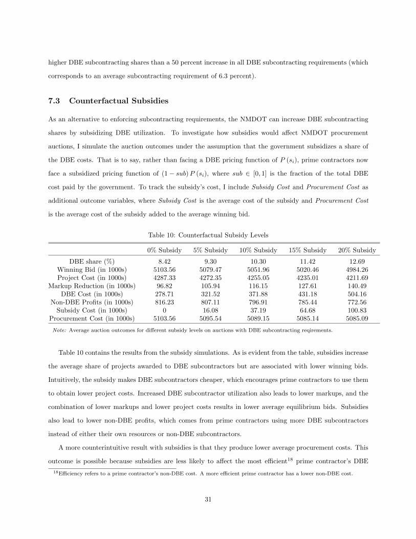
higher DBE subcontracting shares than a 50 percent increase in all DBE subcontracting requirements (which

corresponds to an average subcontracting requirement of 6.3 percent).

7.3 Counterfactual Subsidies

As an alternative to enforcing subcontracting requirements, the NMDOT can increase DBE subcontracting

shares by subsidizing DBE utilization. To investigate how subsidies would affect NMDOT procurement

auctions, I simulate the auction outcomes under the assumption that the government subsidizes a share of

the DBE costs. That is to say, rather than facing a DBE pricing function of P (si), prime contractors now

face a subsidized pricing function of (1− sub)P (si), where sub ∈ [0, 1] is the fraction of the total DBE

cost paid by the government. To track the subsidy’s cost, I include Subsidy Cost and Procurement Cost as

additional outcome variables, where Subsidy Cost is the average cost of the subsidy and Procurement Cost

is the average cost of the subsidy added to the average winning bid.

Table 10: Counterfactual Subsidy Levels

0% Subsidy 5% Subsidy 10% Subsidy 15% Subsidy 20% Subsidy

DBE share (%) 8.42 9.30 10.30 11.42 12.69Winning Bid (in 1000s) 5103.56 5079.47 5051.96 5020.46 4984.26Project Cost (in 1000s) 4287.33 4272.35 4255.05 4235.01 4211.69

Markup Reduction (in 1000s) 96.82 105.94 116.15 127.61 140.49DBE Cost (in 1000s) 278.71 321.52 371.88 431.18 504.16

Non-DBE Profits (in 1000s) 816.23 807.11 796.91 785.44 772.56Subsidy Cost (in 1000s) 0 16.08 37.19 64.68 100.83

Procurement Cost (in 1000s) 5103.56 5095.54 5089.15 5085.14 5085.09

Note: Average auction outcomes for different subsidy levels on auctions with DBE subcontracting reqirements.

Table 10 contains the results from the subsidy simulations. As is evident from the table, subsidies increase

the average share of projects awarded to DBE subcontractors but are associated with lower winning bids.

Intuitively, the subsidy makes DBE subcontractors cheaper, which encourages prime contractors to use them

to obtain lower project costs. Increased DBE subcontractor utilization also leads to lower markups, and the

combination of lower markups and lower project costs results in lower average equilibrium bids. Subsidies

also lead to lower non-DBE profits, which comes from prime contractors using more DBE subcontractors

instead of either their own resources or non-DBE subcontractors.

A more counterintuitive result with subsidies is that they produce lower average procurement costs. This

outcome is possible because subsidies are less likely to affect the most efficient18 prime contractor’s DBE

18Efficiency refers to a prime contractor’s non-DBE cost. A more efficient prime contractor has a lower non-DBE cost.

31

subcontracting decisions yet make every competing firm more competitive. To illustrate this point with an

example, consider a firm that is so efficient that it would never use DBE subcontractors – even with the

subsidy. If that firm wins, there would be no subsidy cost, but the firm would have to lower its markup to

compete with the other firms that can now obtain lower project costs with the subsidy.19

7.4 Comparing Quotas and Subsidies

With the set of outcomes established for different quota and subsidy levels, I now shift my analysis towards

comparing these policies. In particular, I compare outcomes under a subsidy and a quota constrained to

match the average DBE share obtained by the past subcontracting requirements. I calculate these subsidy

and quota levels by using cubic splines to interpolate the non-simulated outcomes.

Table 11: Policy ComparisonsQuota Subsidy

∆ Winning Bid (%) 0.156 -0.595∆ DBE Cost (%) 5.187 -1.585

∆ Non-DBE Profits (%) 0.178 0.005∆ Procurement Cost (%) 0.156 -0.375

Note: Percent change in the average auction outcomesfor policies that achieve the baseline average DBE sub-contracting share.

Table 11 contains the policy comparisons. In general, many of the outcomes under subsidies and quotas

are similar to the outcomes with subcontracting requirements. Subsidies result in lower winning bids, higher

non-DBE profits, and lower procurement costs relative to subcontracting requirements, but subsidies also

result in lower payments to DBE subcontractors. These results are intuitive, since subsidies distort more

efficient prime contractors’ DBE subcontracting decisions less than subcontracting requirements do, and more

efficient prime contractors are more likely to win. Relative to subcontracting requirements and subsidies,

quotas lead to higher payments to DBE subcontractors because prime contractors must use the specified

share of DBEs instead of paying the fine or not using the subsidy, even if DBEs are unusually more costly.

Taken together, these results suggest that quotas are appropriate for governments aiming to increase the

amount of money given to DBE subcontractors, while subsidies are best for governments pursuing policies

with lower procurement costs.

19I explore this result using simulations in the appendix; see appendix F.

32

8 Conclusion

This paper theoretically and empirically examines how subcontracting requirements affect government pro-

curement auctions. The subcontracting policy requires that prime contractors select subcontractors from a

common pool of preferred firms, leading to a shared component in their project costs. Theoretically, this

shared cost component reduces markups, and the reduction in markups can be sufficiently high to mitigate

cost increases from using more costly subcontractors.

The policy experiments illustrate the impact of subcontracting requirements on procurement in New

Mexico. I estimate that New Mexico’s past subcontracting requirements increased the money given to DBE

subcontractors by 12.7 percent, increased procurement costs by only 0.3 percent, and decreased non-DBE

profits by only 0.8 percent. These results suggest that New Mexico’s subcontracting requirements, although

effective in increasing DBE subcontractor utilization, was not responsible for large increases in procurement

costs.

References

Susan Athey. Single crossing properties and the existence of pure strategy equilibria in games of incomplete

information. Econometrica, 64(4):861 – 889, July 2001.

Susan Athey, Dominic Coey, and Jonathan Levin. Set-asides and subsidies in auctions. American Economic

Journal: Microeconomics, 5(1):1–27, 2013.

Nicola Branzoli and Francesco Decarolis. Entry and subcontracting in public procurement auctions. Man-

agement Science, 61(12):2945–2962, 2015.

Dakshina G. De Silva, Timothy Dunne, Georgia Kosmopoulou, and Carlos Lamarche. Disadvantaged busi-

ness enterprise goals in government procurement contracting: An analysis of bidding behavior and costs.

International Journal of Industrial Organization, 30:377–388, 2012.

Dakshina G. De Silva, Timothy P. Hubbard, and Georgia Kosmopoulou. Efficacy of a bidder training program:

Lessons from linc. Working Paper, October 2015.

Dakshina G. De Silva, Georgia Kosmopoulou, and Carlos Lamarche. Subcontracting and the survival of

plants in the road construction industry: A panel quantile regression analysis. Working Paper, April 2016.

33

Richard Gil and Justin Marion. Self-enforcing agreements and relational contracting: Evidence from california

highway procurement. The Journal of Law, Economics, & Organization, 29(2):239 – 277, April 2013.

Christian Gourieroux, Alain Monfort, and Eric Renault. Indirect inference. Journal of Applied Econometrics,

8:S85 – S118, December 1993.

Timothy P. Hubbard and Harry J. Paarsch. Investigating bid preferences at low-price, sealed-bid auctions

with endogenous participation. International Journal of Industrial Organization, 27:1–14, 2009.

Przemyslaw Jeziorski and Elena Krasnokutskaya. Dynamic auction environment with subcontracting. RAND

Journal of Economics, 47(4):751–791, Winter 2016.

Paul L. Joskow. Contract duration and relationship-specific investments: Empirical evidence from coal

markets. American Economic Review, 77(1):168 – 185, March 1987.

Ryan Kellogg. Learning by drilling: Inter-firm learning and relationship persistence in the texas oilpatch.

Quarterly Journal of Economics, 126(4):1961 – 2004, 2011.

Elena Krasnokutskaya and Katja Seim. Bid preference programs and participation in highway procurement

auctions. American Economic Review, 101:2653–2686, October 2011.

Bernard Lebrun. Uniqueness of the equilibrium in first-price auctions. Games and Economic Behavior, 55:

131–151, 2006.

Tong Li and Xiaoyong Zheng. Entry and competition effects in first-price auctions: Theory and evidence

from procurement auctions. Review of Economic Studies, 76(4):1397–1429, 2009.

Justin Marion. Are bid preferences benign? the effect of small business subsidies in highway procurement

auctions. Journal of Public Economics, 91:1591–1624, January 2007.

Justin Marion. How costly is affirmative action? government contracting and california’s proposition 209.

The Review of Economics and Statistics, 91(3):503–522, August 2009.

Justin Marion. Affirmative action and the utilization of minority- and women-owned business in highway

procurement. Economic Inquiry, 49(3):899–915, July 2011.

Justin Marion. Sourcing from the enemy: Horizontal subcontracting in highway procurement. The Journal

of Industrial Economics, 63(1):100 – 128, March 2015.

34

Justin Marion. Affirmative action exemptions and capacity constrained firms. American Economic Journal:

Economic Policy, 9(3):377–407, August 2017.

Scott E. Masten. The organization of production: Evidence from the aerospace industry. The Journal of

Law & Economics, 27(2):403 – 417, October 1984.

Paul Milgrom and Ilya Segal. Envelope theorems for arbitrary choice sets. Econometrica, 70(2):583 – 601,

March 2002.

Daniel P. Miller. Subcontracting and competitive bidding on incomplete procurement contracts. The RAND

Journal of Economics, 45(4):705 – 746, 2014.

Luigi Moretti and Paola Valbonesi. Subcontracting in public procurement: An empirical investigation.

Working Paper, March 2012.

Jun Nakabayashi. Small business set-asides in procurement auctions: an empirical analysis. Journal of Public

Economics, 100:28–44, 2013.

Jun Nakabayashi and Naoki Watanabe. An experimental study of bidding behavior in subcontract auctions.

Tsukuba Economics Working Papers No. 2010-009, December 2010.

Consultant Services Procedures Manual. New Mexico Department of Transportation, July 2014.

http://dot.state.nm.us/en/Program Management.html.

Disadvantaged Business Enterprise Program Manual. New Mexico Department of Transportation Office of

Equal Opportunity Programs, February 2012. http://dot.state.nm.us/en/OEOP.html#c.

OECD. Government at a glance 2015. OECD publishing, Paris, 2015. doi: http://dx.doi.org/10.1787/

gov glance-2015-en.

Iowa Department of Transportation. ”IADOT January 19, 2011 – DBE Commitments”, January 2011. URL

https://www.bidx.com/ia/letting?lettingid=11%2F01%2F19. (accessed October 5, 2017).

Philip J. Reny and Shmuel Zamir. On the existence of pure strategy monotone equilibria in asymmetric

first-price auctions. Econometrica, 72(4):1105–1125, July 2004.

Benjamin Rosa. Resident bid preference, affiliation, and procurement competition: Evidence from new

mexico. MPRA Working Paper, July 2016.

35

Anthony A. Smith. Estimating nonlinear time-series models using simulated vector autoregressions. Journal

of Applied Econometrics, 8:S63 – S84, 1993.

A Proofs

A.1 Properties of the Optimal DBE Subcontracting Decision

A.1.1 Second-Order Conditions

The sufficient condition on optimal DBE subcontracting is given by the following expression:

−P ′′ (si)− ϕ′′ (si; s) < 0.

Observe that this condition is satisfied by the convexity assumption on ϕ and P .

A.1.2 Comparative Statics

The concern here is in understanding how the optimal DBE subcontracting share changes with ci. Differen-

tiating equation (2) while taking into account the optimal DBE subcontracting strategy yields

1 = P ′′ (s (ci; s)) s′ (ci; s) + ϕ′′ (s (ci; s) ; s) s′ (ci; s) .

After some algebraic manipulation, the above equation reduces to

s′ (ci; s, τt) =1

P ′′ (s (ci; s)) + ϕ′′ (s (ci; s) ; s),

which is increasing given the second-order conditions.

A.2 Derivation of the Bid Function (Proposition 1)

I derive the bid function from an envelope theorem argument. In particular, the profit a bidder gains from

a non-DBE cost realization ci is

36

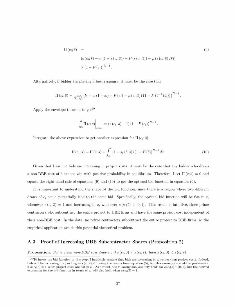
Π (ci; s) = (9)

(b (ci; s)− ci (1− s (ci; s))− P (s (ci; s))− ϕ (s (ci; s) ; s))

× (1− F (ci))N−1

.

Alternatively, if bidder i is playing a best response, it must be the case that

Π (ci; s) = maxbi,si

(bi − ci (1− si)− P (si)− ϕ (si; s))(1− F

(b−1 (bi)

))N−1.

Apply the envelope theorem to get20

d

dcΠ (c; s)

∣∣∣∣c=ci

= (s (ci; s)− 1) (1− F (ci))N−1

.

Integrate the above expression to get another expression for Π (ci; s):

Π (ci; s) = Π (c; s) +

∫ c

ci

(1− st (c; s)) (1− F (c))N−1

dc. (10)

Given that I assume bids are increasing in project costs, it must be the case that any bidder who draws

a non-DBE cost of c cannot win with positive probability in equilibrium. Therefore, I set Π (c; s) = 0 and

equate the right hand side of equations (9) and (10) to get the optimal bid function in equation (6).

It is important to understand the shape of the bid function, since there is a region where two different

draws of ci could potentially lead to the same bid. Specifically, the optimal bid function will be flat in ci

whenever s (ci; s) = 1 and increasing in ci whenever s (ci; s) ∈ [0, 1). This result is intuitive, since prime

contractors who subcontract the entire project to DBE firms will have the same project cost independent of

their non-DBE cost. In the data, no prime contractors subcontract the entire project to DBE firms, so the

empirical application avoids this potential theoretical problem.

A.3 Proof of Increasing DBE Subcontractor Shares (Proposition 2)

Proposition. For a given non-DBE cost draw ci, if s (ci; 0) 6= s (ci; s), then s (ci; 0) < s (ci; s).

20To invert the bid function in this step, I implicitly assume that bids are increasing in ci rather than project costs. Indeed,bids will be increasing in ci so long as s (ci; s) < 1 using the results from equation (5), but this assumption could be problematicif s (ci; s) = 1, since project costs are flat in ci. As a result, the following analysis only holds for s (ci; s) ∈ [0, 1), but the derivedexpression for the bid function in terms of ci will also hold when s (ci; s) = 1.

37

Proof. By the first-order conditions on optimal DBE subcontracting,

ci = P ′ (si) + ϕ′ (si; s) .

Given the assumption s (ci; 0) 6= s (ci; s), it must be the case that ϕ′ (si; s) < 0. When that inequality

holds, prime contractors find it optimal to increase their DBE shares si when there is a DBE subcontracting

requirement. There are now three possible cases for s (ci; 0) and s (ci; s)21: both solutions are interior

solutions, one of the two solutions is an interior solution while the other is a corner solution, or both solutions

occur at different corners. In either of these three cases s (ci; 0) < s (ci; s).

A.4 Proof of Weakly Higher Project Costs (Corollary 1)

Corollary. DBE subcontracting requirements weakly raise project costs.

Proof. Suppose bidder i wins an auction with a bid of b. Without subcontracting requirements, he would

choose shares, s (ci; 0), such that

s (ci; 0) ∈ arg maxsib− ci (1− si)− P (si) ,

or analogously,

s (ci; 0) ∈ arg minsici (1− si)− P (si) .

Define C (si; 0) = ci (1− si)+P (si) as the project cost of bidder i when there are no DBE subcontracting

requirements, and consider the optimal share with subcontracting requirements, s (ci; s). Since s (ci; 0) is

the minimizer of C (·; 0), C (s (ci; 0) ; 0) ≤ C (s (ci; s) ; 0). Since fines are non-negative, C (s (ci; s) ; 0) ≤

C (s (ci; s) ; 0) + ϕ (s (ci; s) ; s) = φ (ci; s).

A.5 Proof of Weakly Lower Markups (Corollary 2)

Corollary. DBE subcontracting requirements weakly lower markups.

Proof. Proposition 2 implies that s (ci; 0) ≤ s (ci; s) for all non-DBE costs, ci. Therefore, markups are weakly

21Since prime contractors find it optimal to increase the share when there is a requirement, any case where s (ci; 0) > s (ci; s)is not possible. The assumption that s (ci; 0) 6= s (ci; s) rules out the cases where both solutions occur at the same corner.

38

lower with DBE subcontracting requirements, since

∫ c

ci

(1− s (c; s)) (1− F (c))N−1

dc ≤∫ c

ci

(1− s (c; 0)) (1− F (c))N−1

dc.

B Microfoundations for the DBE Pricing Function

My theoretical model takes the DBE pricing function as given in its formulation of the optimal bidding and

DBE subcontracting strategies. Theoretically, the DBE pricing function can arise from a variety of different

market structures, each unique to the required work. This section explores two different types of market

structures and derives their respective DBE pricing functions. Throughout this section, DBE subcontractors

will have a thrice continuously differentiable cost function C : [0, 1] → R, which maps the requested share

of work into a cost for the subcontractors. I will refer to that cost function as the DBE cost function.

Furthermore, I assume that C ′, C ′′, C ′′′ > 0 so that the DBE cost function will result in an increasing and

convex DBE pricing function consistent with the pricing function presented in the paper.

Perfect Competition

Some projects may have DBE subcontractors that behave competitively as price takers. For these projects,

DBE subcontractors solve the following profit maximization problem:

maxs≥0

Ps− C (s) .

The first-order conditions generate the following relationship between prices and costs:

P (s) = C ′ (s) .

In other words, the DBE pricing function reflects the marginal cost of the DBE subcontractors.

Monopoly

In contrast to the competitive case, there may be some projects where there is only one DBE subcontractor

in the market. This DBE firm will then behave as a monopolist, solving the following profit maximization

39

problem:

maxs≥0

P (s) s− C (s) .

The monopolist’s pricing decision that arises from its first-order conditions can be written as

P (s) =1

1 + 1ε

C ′ (s) ,

where ε = ds/sdP/P is the price elasticity of demand in the market for that DBE’s services. In words, the

DBE pricing function represents the monopolist’s markup over its marginal cost.22 Note here that not all

market demand functions will result in a one-to-one relationship between prices and DBE shares; a sufficient

condition for this relationship to be a function is that the market demand’s elasticity is constant.

C Estimation Appendix

In order to maintain desirable properties of the model across different parameter guesses, I must restrict

the model’s set of possible parameter values. I include these restrictions along with details on the optimal

weighting matrix and asymptotic standard errors in this appendix.

C.1 Parametric Restrictions

I restrict the parameters so that the pricing function is convex and increasing in the DBE share and the

fine function is convex and non-increasing in the share. To illustrate these restrictions, consider the first and

second-order conditions of the DBE pricing function and the fine function for any given auction:

P ′ (si) =

(α0 + α1si + α2

si1− si

+ α′3zw + uw

)xw +

(α1 +

α2

(1− si)2

)sixw

ϕ′ (si; s) =

2γ (si − s) x if si < s

0 if si ≥ s

22Observe that I implicitly assume that the monopolist firm does not strategically take the fine function into considerationwhen determining its prices.

40

P ′′ (si) = 2

(α1 +

α2

(1− si)2

)xw +

(2α2

(1− si)3

)sixw

ϕ′′ (si; s) =

2γx if si < s

0 if si ≥ s.

Observe that restricting α0 > 0, α1 > 0, α2 > 0 and α3 > 0 will generate a DBE pricing function that

is convex and increasing in the DBE share for si ∈ [0, 1). Similarly, restricting γ > 0 will produce a fine

function that is convex and non-increasing for si ∈ [0, 1]. In estimation, I restrict the structural parameter

values to the aforementioned range of possible values to maintain those properties across parameter guesses.

C.2 Standard Errors and Optimal Weighting Matrix

Following Gourieroux et al. (1993), the asymptotic distribution of the indirect inference estimator takes the

following form:

√W(θHW − θ0

)d−→ N (0, Vθ)

with

Vθ =

(1 +

1

H

)(D′ΩD)

−1D′ΩVβ0

ΩD (D′ΩD)−1,

D =∂β0

∂θ′0,

and

√W(βHW − β0

)d−→ N (0, Vβ0

) .

Notation wise, θHW are the structural parameters estimated from the data, θ0 are the true structural

parameters, Ω is a positive definite weighting matrix, β0 are the auxiliary parameters evaluated using the

true structural parameters, andd−→ denotes convergence in distribution. The optimal weight matrix in this

setting is Ω? = (Vβ0)−1

, yielding an asymptotic variance of Vθ =(1 + 1

H

)(D′Ω?D)

−1.

In practice, I replace the objects of the asymptotic distribution by consistent estimators. Specifically, I

41

use the following consistent estimators in place of their asymptotic counterparts:

D =∂βHW

(θHW

)∂θ′HW

and

Ω? =(VβHW (θHW )

)−1

.

In constructing VβHW (θHW ), the estimator for Vβ0, I use a parametric bootstrap procedure.

D Estimated Pricing and Fine Functions

DBE Subcontractor Share0 0.05 0.1 0.15 0.2 0.25 0.3 0.35 0.4 0.45 0.5

Pric

e (F

ract

ion

of th

e E

ngin

eer's

Est

imat

e)

0

0.1

0.2

0.3

0.4

0.5

0.6

0.7

0.8

Figure 5: The DBE Pricing Function as a Fraction of the Engineer’s Estimate

Note: This figure shows a plot of the price of using DBE subcontractors as a fraction of the engineer’s estimate,which corresponds to the expression P (si)

x. Here, the pricing function is evaluated using the mean level of subprojects

in the DBE-eligible data and the mean level of the unobservable pricing shock term (σu) when there is an establishedDBE subcontracting requirement of 7.5 percent.

42

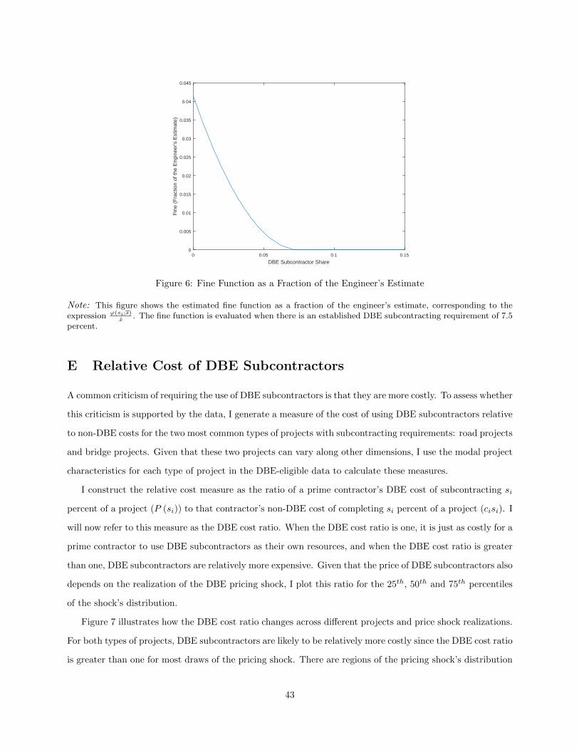
DBE Subcontractor Share0 0.05 0.1 0.15

Fin

e (F

ract

ion

of th

e E

ngin

eer's

Est

imat

e)

0

0.005

0.01

0.015

0.02

0.025

0.03

0.035

0.04

0.045

Figure 6: Fine Function as a Fraction of the Engineer’s Estimate

Note: This figure shows the estimated fine function as a fraction of the engineer’s estimate, corresponding to theexpression ϕ(si;s)

x. The fine function is evaluated when there is an established DBE subcontracting requirement of 7.5

percent.

E Relative Cost of DBE Subcontractors

A common criticism of requiring the use of DBE subcontractors is that they are more costly. To assess whether

this criticism is supported by the data, I generate a measure of the cost of using DBE subcontractors relative

to non-DBE costs for the two most common types of projects with subcontracting requirements: road projects

and bridge projects. Given that these two projects can vary along other dimensions, I use the modal project

characteristics for each type of project in the DBE-eligible data to calculate these measures.

I construct the relative cost measure as the ratio of a prime contractor’s DBE cost of subcontracting si

percent of a project (P (si)) to that contractor’s non-DBE cost of completing si percent of a project (cisi). I

will now refer to this measure as the DBE cost ratio. When the DBE cost ratio is one, it is just as costly for a

prime contractor to use DBE subcontractors as their own resources, and when the DBE cost ratio is greater

than one, DBE subcontractors are relatively more expensive. Given that the price of DBE subcontractors also

depends on the realization of the DBE pricing shock, I plot this ratio for the 25th, 50th and 75th percentiles

of the shock’s distribution.

Figure 7 illustrates how the DBE cost ratio changes across different projects and price shock realizations.

For both types of projects, DBE subcontractors are likely to be relatively more costly since the DBE cost ratio

is greater than one for most draws of the pricing shock. There are regions of the pricing shock’s distribution

43

DBE share (si)0 0.05 0.1 0.15 0.2 0.25 0.3 0.35 0.4 0.45 0.5

CostRatio

(

P(s

i)

cisi

)

0.5

1

1.5

2

2.5

3

3.5

4Bridge Project

ulow

umedium

uhigh

DBE share (si)0 0.05 0.1 0.15 0.2 0.25 0.3 0.35 0.4 0.45 0.5

CostRatio

(

P(s

i)

cisi

)

0.5

1

1.5

2

2.5

3Road Project

ulow

umedium

uhigh

Figure 7: DBE Cost Ratios

Note: DBE cost ratios for the modal bridge and road construction projects. The vertical axis has the DBE costratio, and the horizontal axis has the DBE share. The different lines correspond to different levels of the unobservedshock on the DBE pricing function, where “low” corresponds to the 25th percentile, “medium” corresponds to the50th percentile, and high corresponds to the 75th percentile of the shock’s distribution.

where DBE subcontractors are less costly, which suggests that DBE utilization is sensitive to the realization

of the shock.

F Subsidy and Quota Simulations

In this section, I repeat the numerical simulations with quotas and subsidies. I maintain the environment

and functional form assumptions from section 4; for completeness, I list those assumptions below:

• N = 2

• ci ∼ U [0, 1], where U [·, ·] denotes the uniform distribution.

• P (si) =ξs2i2

• ϕ (si; s) =

λ(si−s)2

2 if si < s

0, if si ≥ s

• ξ = 2, λ = 3

I set the quota and subsidy to 30% to match the simulations with subcontracting requirements.

Figure 8 shows the DBE subcontracting functions when there is a quota (the left panel) and subsidy

(the right panel) and compares them to the subcontracting functions when there is no policy. For quotas,

44

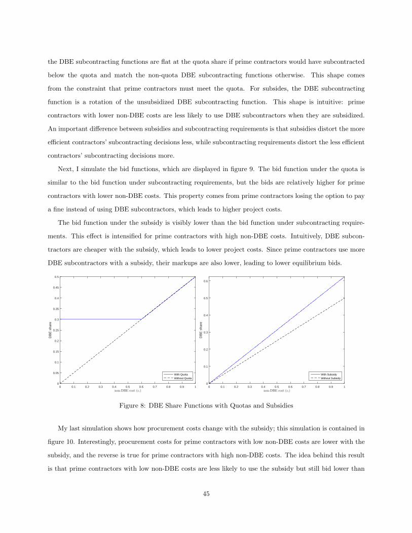
the DBE subcontracting functions are flat at the quota share if prime contractors would have subcontracted

below the quota and match the non-quota DBE subcontracting functions otherwise. This shape comes

from the constraint that prime contractors must meet the quota. For subsides, the DBE subcontracting

function is a rotation of the unsubsidized DBE subcontracting function. This shape is intuitive: prime

contractors with lower non-DBE costs are less likely to use DBE subcontractors when they are subsidized.

An important difference between subsidies and subcontracting requirements is that subsidies distort the more

efficient contractors’ subcontracting decisions less, while subcontracting requirements distort the less efficient

contractors’ subcontracting decisions more.

Next, I simulate the bid functions, which are displayed in figure 9. The bid function under the quota is

similar to the bid function under subcontracting requirements, but the bids are relatively higher for prime

contractors with lower non-DBE costs. This property comes from prime contractors losing the option to pay

a fine instead of using DBE subcontractors, which leads to higher project costs.

The bid function under the subsidy is visibly lower than the bid function under subcontracting require-

ments. This effect is intensified for prime contractors with high non-DBE costs. Intuitively, DBE subcon-

tractors are cheaper with the subsidy, which leads to lower project costs. Since prime contractors use more

DBE subcontractors with a subsidy, their markups are also lower, leading to lower equilibrium bids.

non-DBE cost (ci)0 0.1 0.2 0.3 0.4 0.5 0.6 0.7 0.8 0.9 1

DB

E s

hare

0

0.05

0.1

0.15

0.2

0.25

0.3

0.35

0.4

0.45

0.5

With QuotaWithout Quota

non-DBE cost (ci)0 0.1 0.2 0.3 0.4 0.5 0.6 0.7 0.8 0.9 1

DB

E s

hare

0

0.1

0.2

0.3

0.4

0.5

0.6

With SubsidyWithout Subsidy

Figure 8: DBE Share Functions with Quotas and Subsidies

My last simulation shows how procurement costs change with the subsidy; this simulation is contained in

figure 10. Interestingly, procurement costs for prime contractors with low non-DBE costs are lower with the

subsidy, and the reverse is true for prime contractors with high non-DBE costs. The idea behind this result

is that prime contractors with low non-DBE costs are less likely to use the subsidy but still bid lower than

45

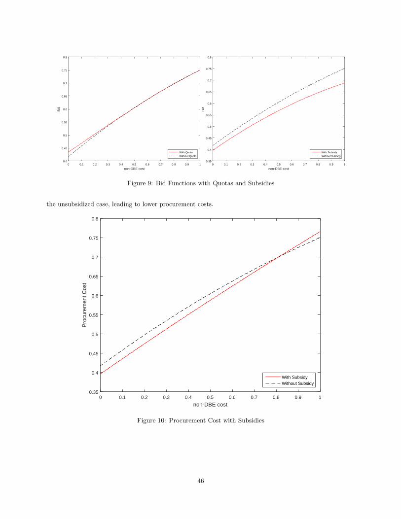
non-DBE cost0 0.1 0.2 0.3 0.4 0.5 0.6 0.7 0.8 0.9 1

Bid

0.4

0.45

0.5

0.55

0.6

0.65

0.7

0.75

0.8

With QuotaWithout Quota

non-DBE cost0 0.1 0.2 0.3 0.4 0.5 0.6 0.7 0.8 0.9 1

Bid

0.35

0.4

0.45

0.5

0.55

0.6

0.65

0.7

0.75

0.8

With SubsidyWithout Subsidy

Figure 9: Bid Functions with Quotas and Subsidies

the unsubsidized case, leading to lower procurement costs.

non-DBE cost0 0.1 0.2 0.3 0.4 0.5 0.6 0.7 0.8 0.9 1

Pro

cure

men

t Cos

t

0.35

0.4

0.45

0.5

0.55

0.6

0.65

0.7

0.75

0.8

With SubsidyWithout Subsidy

Figure 10: Procurement Cost with Subsidies

46

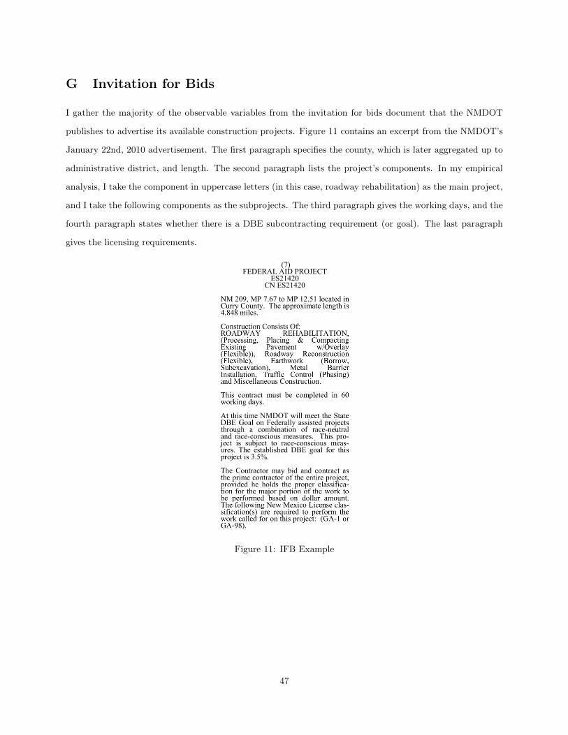
G Invitation for Bids

I gather the majority of the observable variables from the invitation for bids document that the NMDOT

publishes to advertise its available construction projects. Figure 11 contains an excerpt from the NMDOT’s

January 22nd, 2010 advertisement. The first paragraph specifies the county, which is later aggregated up to

administrative district, and length. The second paragraph lists the project’s components. In my empirical

analysis, I take the component in uppercase letters (in this case, roadway rehabilitation) as the main project,

and I take the following components as the subprojects. The third paragraph gives the working days, and the

fourth paragraph states whether there is a DBE subcontracting requirement (or goal). The last paragraph

gives the licensing requirements.

Figure 11: IFB Example

47

H Additional Regressions and Graphs

Note: This figure shows the distribution of non-zero DBE subcontracting requirements.

Note: This figure shows the percentage difference between the share of DBE subcontractors actually used on a givenproject and the DBE subcontracting requirement conditional on the project having a subcontracting requirement.Although there is some bunching at 0 percent, there is a non-trivial mass of projects where contractors exceed thesubcontracting requirement by more than 1 percent. Consequently, a continuous function is used to approximate thechange in incentives induced by having a DBE subcontracting requirement rather than a discrete function. This figureis truncated at 15 percent for visual clarity.

Tables 12 and 13 motivate the main modeling assumptions of the paper. Table 12 contains a regression

specification very similar to the first three columns of tables 2 and 3, but I include a control for firm capacity

(as measured by the project backlog of a firm divided by the maximum backlog of the firm during the sample

period) as an additional observable. This regression motivates the absence of capacity constraints in my

paper’s main analysis; the statistically insignificant coefficient on the capacity measure shows that there is

insufficient descriptive evidence in favor of including firm capacity in firm bidding and DBE subcontracting

decisions. Similarly, table 13 is a regression that explores firm entry decisions as measured by the number of

48

planholders and the fraction of bidders over the number of planholders. Although entry is typically modeled

as an endogenous decision in these types of procurement models, the lack of an economically and statistically

significant coefficient on the DBE requirement variable suggests that entry is not a first-order concern in

evaluating these DBE participation policies.

Table 12: Capacity Regressions

Dependent variable:

log(Winning Bid) DBE Share (%)

(1) (2)

log(Engineer’s Estimate) 0.927∗∗∗ −0.352(0.017) (0.624)

DBE Req (%) 0.002 1.014∗∗∗

(0.004) (0.184)log(Length + 1) 0.043∗∗∗ 0.016

(0.014) (0.511)Capacity −0.019 −0.355

(0.040) (1.161)log(Planholders) 0.007 1.610

(0.056) (1.940)log(Subprojects) 0.049∗ 1.432

(0.028) (0.880)Number of Licenses Required 0.044∗∗ 1.773∗

(0.020) (0.924)log(Working Days) 0.038∗ −0.613

(0.020) (0.605)Bidders −0.018∗∗∗ −0.058

(0.005) (0.215)Federal Highway −0.034 −0.240

(0.022) (0.690)Urban −0.018 1.899∗

(0.034) (0.970)

Observations 389 389Adjusted R2 0.985 0.227

Note: ∗p<0.1; ∗∗p<0.05; ∗∗∗p<0.01Regression includes controls for district and type ofwork as well as month and year fixed effects. Stan-dard errors are robust.

49

Table 13: Entry Regressions

Dependent variable:

Bidders/Planholders Planholders

(1) (2)

log(Engineer’s Estimate) 0.008 1.392∗∗∗

(0.008) (0.353)DBE Req (%) 0.0005 0.105

(0.002) (0.087)log(Length + 1) 0.010 −1.239∗∗∗

(0.006) (0.314)log(Subprojects) −0.001 3.417∗∗∗

(0.016) (0.589)Number of Licenses Required −0.022∗∗ 1.194∗∗∗

(0.009) (0.457)log(Working Days) −0.018∗ 1.554∗∗∗

(0.011) (0.408)Federal Highway 0.001 −0.543

(0.011) (0.429)Urban 0.002 1.522∗∗

(0.016) (0.619)

Observations 389 389Adjusted R2 0.115 0.708

Note: ∗p<0.1; ∗∗p<0.05; ∗∗∗p<0.01Regression includes controls for district and type ofwork as well as month and year fixed effects. Stan-dard errors are robust.

50