submitted to ieee transactions on image …randy/publications/rlm_review/jr2.pdf · bistatic sar,...

SUBMITTED TO IEEE TRANSACTIONS ON IMAGE PROCESSING, MARCH 2003 1

Motion Measurement Errors and Autofocus in

Bistatic SARBrian D. Rigling, Member, IEEE, and Randolph L. Moses Senior Member, IEEE

Abstract

This paper discusses the effect of motion measurement errors (MMEs) on measured bistatic synthetic

aperture radar (SAR) phase history data that has been motion compensated to the scene origin. We

characterize the effect of low frequency MMEs on bistatic SAR images, and based on this characterization,

we derive limits on the allowable MMEs to be used as system specifications. Finally, we demonstrate

that proper orientation of a bistatic SAR image during the image formation process allows application

of monostatic SAR autofocus algorithms in post-processing to mitigate image defocus.

Index Terms

bistatic, SAR, motion measurement errors, ground map, autofocus.

I. INTRODUCTION

Synthetic aperture radar (SAR) imaging is an invaluable tool for aerial ground surveillance. Monostatic

SAR systems, where the transmitting and receiving antennas are located on the same platform and are

frequently the same antenna, have been the subject of a great deal of research and development over

the past few decades. The attraction of monostatic SAR is its relative simplicity, both in system design

and deployment. However, in trying to observe an area of interest at close range, a high cost monostatic

platform may place itself at risk by illuminating hostile regions with its transmissions.

A growing military interest in cost effective UAV technology has sparked renewed interest in bistatic

synthetic aperture radar. Bistatic SAR, as an alternative to monostatic SAR, allows a passive receiving

B.D. Rigling is with the Department of Electrical Engineering, Wright State University, 422 Russ Engineering Center, 3640

Colonel Glenn Highway, Dayton, OH 45435-0001, Email: [email protected], Phone: (937) 775-5100.

R.L. Moses is with the Department of Electrical and Computer Engineering, The Ohio State University, 205 Dreese Labs,

2015 Neil Avenue, Columbus, OH 43210, E-mail:([email protected]).

May 3, 2005 DRAFT


platform to observe at close range a scene illuminated by a remote transmitting platform. The transmitting

platform may in some cases be an illuminator of opportunity, such as an overpassing satellite [1] or a

local commercial transmitter. The receiving platform may be of signicantly reduced cost and is far less

observable due to its passive nature.

Multiple image formation processes have been developed for bistatic SAR including the backprojection

algorithm (BPA) [2], matched filtering (MF) [3], direct Fourier inversion [4], and the polar format

algorithm (PFA) [5]. All of these processes assume that the locations of the transmit and receive platforms

are known perfectly at every point in their flight paths. However, it is well known from operational

monostatic SAR systems that exact motion measurement is impossible to obtain, and a slight motion

measurement error (MME) can have a drastic effect on the quality of the resulting SAR imagery.

In this paper, we analytically characterize the effects of imperfect motion measurement on bistatic

SAR images. This analysis provides bounds that define the necessary precision in platform motion

compensation needed to obtain usable imagery from bistatic SAR phase history data. In addition, we

consider post-processing techniques for correcting MMEs, commonly known as autofocus. We show

that, provided the bistatic SAR images are formed in an appropriately-chosen reference frame, mono-

static autofocus techniques are applicable without modification to bistatic SAR images. In this way, the

significant development in monostatic autofocus methods may be carried over to bistatic image focusing.

Specifically, the bistatic SAR coordinate frame needed to apply monostatic autofocus methods is one

derived via the Taylor series approximation to the bistatic differential range equation (see [5]). This

approximation provides a three-dimensional generalization of the two-dimensional results in [2].

An outline of the paper is as follows. In Section II, we will describe our model for bistatic SAR

phase history data collection. Section III studies how the information recorded during data collection is

interpreted by image formation algorithms. Section IV describes a typical model for low frequency MMEs

and analyzes their effects on the collected phase history data. In Section V, we demonstrate the effect

of MMEs on bistatic SAR images. We also derive bounds on the allowable MMEs, based on limiting

the degree of quadratic phase error, and we show how autofocus techniques that have been developed

for monostatic SAR may be applied to bistatic SAR imagery. Finally, we summarize our conclusions in

Section VI.

II. BISTATIC PHASE HISTORY DATA

Consider the bistatic SAR data collection geometry shown in Figure 1. The center of the scene to

be imaged is located at the origin of coordinates, and the ground plane is the x-y plane. A scatterer

May 3, 2005 DRAFT


t

z

rt

rr

PathTransmitter

PathReceiver

rr (τ)

rm

r

mth Scatterer

y

x

~

~(τ)

(τ)

(τ)

Fig. 1. Top view of a bistatic data collection geometry. The x-y plane is the ground plane.

within that scene is located at rm = (xm, ym, zm). The actual location of the transmitter at a given

time τ is rt(τ) = (xt(τ), yt(τ), zt(τ)). The measured transmitter location at time τ is given by rt(τ) =

rt(τ)+ rt(τ), where rt(τ) = (xt(τ), yt(τ), zt(τ)) is the location measurement error. Similarly, the actual

location of the receiver at a given time τ is rr(τ) = (xr(τ), yr(τ), zr(τ)), and the measured location

of the receiver is rr(τ) = rr(τ) + rr(τ), where rr(τ) = (xr(τ), yr(τ), zr(τ)) is the receiver location

measurement error.

As the transmitter moves along its flight path, the radiating antenna periodically transmits pulses of

energy in the direction of the scene center. Each transmitted pulse travels from the transmitter to the

scene of interest, where it is reflected by scatterers within the area of illumination. This reflected energy

disperses in all directions, and some of this energy is observed by the antenna on the receiving platform.

We assume that the travel time of the pulse from the transmitter to a scatterer to the receiver is sufficiently

short, with respect to the pulse duration, that any platform movement within that time period may be

neglected.

For clarity of exposition, we assume that transmitted pulses have uniform power over the frequency

range f ∈ [f0, f0 + B], where f0 and B represent the lowest frequency and the bandwidth of the

transmitted pulse, respectively. We also assume that scatterers behave as ideal point scatterers within this

frequency band. These assumptions are not critical to the derivations to follow, but they do make for

easier analysis. The effects of a non-uniform transmit spectrum and non-ideal scattering responses may

May 3, 2005 DRAFT


be incorporated into the results of Section III, and we will make a note of this at that point.

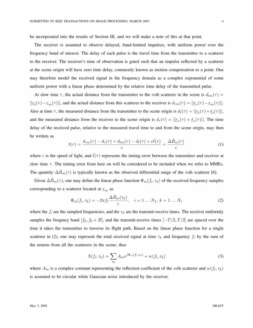
The receiver is assumed to observe delayed, band-limited impulses, with uniform power over the

frequency band of interest. The delay of each pulse is the travel time from the transmitter to a scatterer

to the receiver. The receiver’s time of observation is gated such that an impulse reflected by a scatterer

at the scene origin will have zero time delay, commonly known as motion compensation to a point. One

may therefore model the received signal in the frequency domain as a complex exponential of some

uniform power with a linear phase determined by the relative time delay of the transmitted pulse.

At slow time τ , the actual distance from the transmitter to the mth scatterer in the scene is dtm(τ) =

||rt(τ)−rm(τ)||, and the actual distance from this scatterer to the receiver is drm(τ) = ||rr(τ)−rm(τ)||.Also at time τ , the measured distance from the transmitter to the scene origin is dt(τ) = ||rt(τ)+ rt(τ)||,and the measured distance from the receiver to the scene origin is dr(τ) = ||rr(τ) + rr(τ)||. The time

delay of the received pulse, relative to the measured travel time to and from the scene origin, may then

be written as

t(τ) =drm(τ)− dr(τ) + dtm(τ)− dt(τ) + ct(τ)

c=

∆Rm(τ)c

(1)

where c is the speed of light, and t(τ) represents the timing error between the transmitter and receiver at

slow time τ . The timing error from here on will be considered to be included when we refer to MMEs.

The quantity ∆Rm(τ) is typically known as the observed differential range of the mth scatterer [6].

Given ∆Rm(τ), one may define the linear phase function Φm(fi, τk) of the received frequency samples

corresponding to a scatterer located at rm as

Φm(fi, τk) = −2πfi∆Rm(τk)

c, i = 1 . . . Nf , k = 1 . . . Nτ (2)

where the fi are the sampled frequencies, and the τk are the transmit-receive times. The receiver uniformly

samples the frequncy band [f0, f0 + B], and the transmit-receive times [−T/2, T/2] are spaced over the

time it takes the transmitter to traverse its flight path. Based on the linear phase function for a single

scatterer in (2), one may represent the total received signal at time τk and frequency fi by the sum of

the returns from all the scatterers in the scene; thus

S(fi, τk) =∑m

AmejΦm(fi,τk) + w(fi, τk) (3)

where Am is a complex constant representing the reflection coefficient of the mth scatterer and w(fi, τk)

is assumed to be circular white Gaussian noise introduced by the receiver.

May 3, 2005 DRAFT


III. IMAGE FORMATION

To analyze the effects of MMEs on bistatic SAR imagery, we must first understand how an image

formation algorithm interprets the collected phase history data to form images. The location rm of each

scatterer in the observed scene is encoded in the phase of the observed phase histories via each differential

range function ∆Rm(τ). One typically seeks to form SAR images by assuming that the MMEs are zero

and by assuming that all of the scatterers in a scene lie on a uniform grid of pixel locations. The ML

estimate of the reflectivity of a scatterer at an (x, y, z) pixel location may then be computed by using a

matched filter of the form [5]

P (x, y, z) =1

NfNτ

Nf∑

i=1

Nτ∑

k=1

S(fi, τk)e−jΦxyz(fi,τk) (4)

where Φxyz(fi, τk) represents a phase function linearly dependent on the differential range of a scatterer

located at (x, y, z). To form a complete image, equation (4) is computed for every element of the assumed

grid of (x, y, z) locations on the image plane.

As (4) is computationally inefficient, many image formation algorithms alter the method of computing

the matched filter, or approximate it, in order to reduce the algorithm’s complexity. A Taylor expansion

of the bistatic differential range in (1) gives the first order approximation (commonly called the far-field

approximation [5])

∆R ≈ −xxt + yyt + zzt√x2

t + y2t + z2

t

− xxr + yyr + zzr√x2

r + y2r + z2

r

. (5)

By introducing the variables φt and φr (θt and θr), denoting the azimuth (elevation) angles of the

transmitter and receiver with respect to the scene center, we can write (5) in terms of these angles as

∆R(τk) ≈ −x cos(φt(τk)) cos(θt(τk))

−y sin(φt(τk)) cos(θt(τk))

−z sin(θt(τk))− x cos(φr(τk)) cos(θr(τk))

−y sin(φr(τk)) cos(θr(τk))− z sin(θr(τk)) (6)

where we include the dependence on the sampled slow time τk. This allows use of the approximate

matched filter [5]

P (x, y, z) ≈ 1NfNτ

Nf∑

i=1

Nτ∑

k=1

S(fi, τk)

· exp{−j

4π

c[xfx(fi, τk) + yfy(fi, τk) + zfz(fi, τk)]

}(7)

May 3, 2005 DRAFT


where

fx(fi, τk) =fi

2[cos(φt(τk)) cos(θt(τk))

+ cos(φr(τk)) cos(θr(τk))],

fy(fi, τk) =fi

2[sin(φt(τk)) cos(θt(τk))

+ sin(φr(τk)) cos(θr(τk))],

fz(fi, τk) =fi

2[sin(θt(τk)) + sin(θr(τk))]. (8)

Note that use of the far-field assumption in equation (6) introduces distortion and defocus into the final

image. To limit the degree of defocus experienced, one typically limits the maximum size of an imaged

scene [5]. Setting z = 0 (for a ground plane image) and defining the rotation of coordinates

f ′x = fx cos(φb) + fy sin(φb)

f ′y = −fx sin(φb) + fy cos(φb) (9)

and

x′ = x cos(φb) + y sin(φb)

y′ = −x sin(φb) + y cos(φb), (10)

where the bistatic look angle (shown in Figure 2) is

φb = arctan(

fy(fi, τkb)

fx(fi, τkb)

)

= arctan(

sin φt cos θt + sin φr cos θr

cos φt cos θt + cos φr cos θr

), (11)

we obtain

P (x, y, 0) ≈ 1NfNτ

Nf∑

i=1

Nτ∑

k=1

S(fi, τk)

· exp{−j

4π

c[x′f ′x(fi, τk) + y′f ′y(fi, τk)]

}. (12)

We then resample the data onto the rectangular grid defined by

f ′x = f0 + Bxkx

Nx, kx = 0 . . . Nx − 1

and f ′y =−By

2+ By

ky

Ny, ky = 0 . . . Ny − 1 (13)

May 3, 2005 DRAFT


to obtain

P (x′, y′, 0) ≈ 1NxNy

Nx−1∑

kx=0

Ny−1∑

ky=0

S(kx, ky)

· exp{−j

4π

c

[x′

(f0 + Bx

kx

Nx

)

+y′(−By

2+ By

ky

Ny

)]}(14)

In (11), φt and φr (θt and θr) represent the azimuth (elevation) angles of the transmitter and receiver at

their corresponding aperture midpoints.

One may also assume that the far-field assumption holds for the observed phase history data, such that

the coordinate system rotation and polar-to-rectangular interpolation converts equation (3) into the form

(omitting the noise term)

S(kx, ky) ≈∑m

Amej 4π

c

hx′m�

f0+BxkxNx

�+y′m

�−By

2+By

ky

Ny

�i(15)

where (x′m, y′m) is the location of the mth scatterer in the rotated coordinate system defined by (10).

Thus, applying the approximate matched filter (14) to (15) yields

P (x′, y′, 0) ≈∑m

Amej 2π

c

h(x′−x′m)(2f0+Bx−Bx

Nx)−(y′−y′m)

By

Ny

i

·sin

(2π(x′−x′m)Bx

c

)

sin(

2π(x′−x′m)Bx

cNx

)

sin

(2π(y′−y′m)By

c

)

sin(

2π(y′−y′m)By

cNy

) , (16)

provided that there are no MMEs. We see from (16) that the scatterer location information, encoded

in the observed phase histories by the differential range, determines the location of the Dirichlet kernel

functions (the [sin(·)/ sin(·)] functions in (16)) in the image, and the width and breadth of these functions

are determined by the bandwidths Bx and By of the phase history data.

Equation (16) is derived assuming both uniform transmit power in the frequency band [f0, f0 + B]

and flat scattering center responses. If a non-uniform transmit spectrum is used, or if scattering centers

have frequency dependent responses, the resulting matched filter response will be similar to (16), but the

Dirichlet kernel functions will be replaced by responses corresponding to the non-uniform spectrum and

non-ideal returns. The locations of these responses in the final image, however, are still determined by

the scatterer location information encoded in the observed differential range functions.

To understand the effects of MMEs in our data collection, we study the manner in which the scatterer

location information is encoded in the differential range function. We first assume that the ground range

rt =√

xt(τ)2 + yt(τ)2 and the slant range Rt =√

xt(τ)2 + yt(τ)2 + zt(τ)2 of the transmitter are

May 3, 2005 DRAFT


sufficiently large such that they may be treated as constants with respect to slow time τ . We make the

same assumption about the ground range and slant range of the receiver, rr =√

xr(τ)2 + yr(τ)2 and

Rr =√

xr(τ)2 + yr(τ)2 + zr(τ)2. Finally, we assume that the transmitter and receiver traverse linear

flight paths at constant velocities. This allows us to write cosφ(τ) = (xt+vxtτ)/rt and cos θ(τ) = rt/Rt,

as well as similar substitutions for the other expressions in (6). Thus, the approximated differential range

in (6) may be further approximated by a linear function of slow time

∆R(τ) ≈ −x

(xt + vxtτ

rt

)(rt

Rt

)− y

(yt + vytτ

rt

)(rt

Rt

)− z

(zt + vztτ

Rt

)

−x

(xr + vxrτ

rr

)(rr

Rr

)− y

(yr + vyrτ

rr

)(rr

Rr

)− z

(zr + vzrτ

Rr

)

=[−x

(xt

Rt+

xr

Rr

)− y

(yt

Rt+

yr

Rr

)− z

(zt

Rt+

zr

Rr

)]

[−x

(vxt

Rt+

vxr

Rr

)− y

(vyt

Rt+

vyr

Rr

)− z

(vzt

Rt+

vzr

Rr

)]τ

, +β0 + β1τ. (17)

The locations of the transmitter and receiver at their aperture midpoints are given by (xt, yt, zt) and

(xr, yr, zr), and the transmitter and receiver velocity vectors are (vxt, vyt, vzt) and (vxr, vyr, vzr), respec-

tively.

Equation (17) describes a transformation which relates the linear approximation of the differential

range ∆R(τ) = β0 + β1τ to the actual location of a scatterer in the scene, which is written as

β0

β1

=

− xt

Rt− xr

Rr− yt

Rt− yr

Rr− zt

Rt− zr

Rr

−vxt

Rt− vxr

Rr−vyt

Rt− vyr

Rr−vzt

Rt− vzr

Rr

x

y

z

. (18)

We will focus on scatterers located on the ground plane (z = 0), giving β0

β1

=

− xt

Rt− xr

Rr− yt

Rt− yr

Rr

−vxt

Rt− vxr

Rr−vyt

Rt− vyr

Rr

x

y

, Q

x

y

. (19)

Therefore, given a measured differential range function for a single scatterer on the ground, one may

linearly approximate ∆R(τ) and then use x

y

= Q−1

β0

β1

(20)

to estimate the (x, y) location of that scatterer’s response, as defined by (16), in a ground plane image.

From (16) and (19), we make two important observations. First, from (16) we see that the accuracy

with which we may extract location information from the recorded phase histories is determined by the

May 3, 2005 DRAFT


Bistatic aspect

tφ

φr

bφ

rθ

tθ

x’

x

y

z

Transmitter aspect

Receiver aspect

Fig. 2. The bistatic aspect bisects the solid angle between the transmitter and receiver aspects in three-dimensional space.

bandwidths of the data in range (Bx) and crossrange (By). Second, provided there are no MMEs, the

(x, y) location of a scatterer in the ground plane is encoded in the differential range (β0 = ∆R(τ)) and

its time derivative (β1 = ∆R′(τ)) at every point in the data collection through the linear mapping Q.

IV. CHARACTERIZING MOTION MEASUREMENT ERRORS

The above derivations assume that there are no MMEs. To implement an actual bistatic SAR system,

MMEs must be considered. Errors in measuring the motion of an airborne surveillance platform have

frequently been characterized [6]–[9] by expressions in the form

r(τ) = g(τ) + h(τ) (21)

where g(τ) represents low frequency errors, and h(τ) represents high frequency errors. The low frequency

component of the errors is often modeled as a polynomial, whereas the high frequency errors are more

difficult to model and are most often described by their spectral characteristics or RMS values. The high

frequency errors are usually much smaller in magnitude than the low frequency errors, and typically

consist of noise-like elements, and sinusoidal components with periods much shorter than the aperture

duration. Errors not due to motion measurement, such as propagation phenomena and atmospheric

turbulence, also contribute to the high frequency errors. We will focus on the dominant low frequency

elements of the unmeasured platform motion, and we will model them with a quadratic polynomial in

May 3, 2005 DRAFT


the form

g(τ) =

x(τ)

y(τ)

z(τ)

=

px

py

pz

+

vx

vy

vz

τ +

ax

ay

az

τ2

2(22)

where [px py pz]T represents the error in measuring the platform’s location at the aperture midpoint,

and [vx vy vz]T and [ax ay az]T represent the errors in measuring the platform’s velocity and

acceleration.

By applying to ∆R(τ) the same approximations used to arrive at (17), we can approximate the error

introduced into the observed differential range as

∆R(τ) ≈ −xt(τ)xt + vxtτ

Rt− xr(τ)

xr + vxrτ

Rr

−yt(τ)yt + vytτ

Rt− yr(τ)

yr + vyrτ

Rr

−zt(τ)zt + vztτ

Rt− zr(τ)

zr + vzrτ

Rr+ ct(τ). (23)

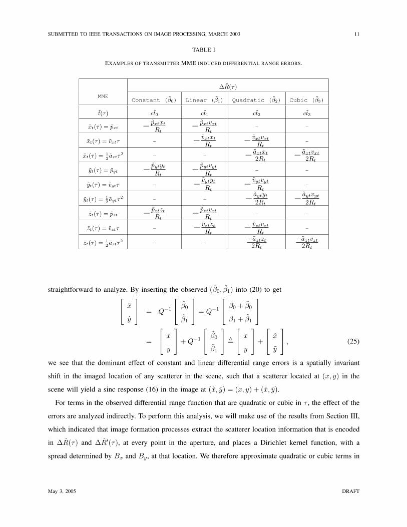
Using (23), we may characterize the effect of motion measurement errors on the observed differential

range, by substituting in the quadratic polynomial expressions for the MMEs {xt(τ), xr(τ), yt(τ), yr(τ), zt(τ), zr(τ)}in (22). In addition, we will assume that the time synchronization error between the transmit and receive

platforms is of the form t(τ) = t0 + t1τ + t2τ2 + t3τ

3. The result is a cubic polynomial expression

for (23), ∆R(τ) ≈ β0 + β1τ + β2τ2 + β3τ

3. Table I shows the errors in the observed differential range

induced by transmitter MMEs and time synchronization errors. The errors induced by receiver MMEs

are identical. In Section V, the results in Table I will allow us to study the effect of MMEs on bistatic

SAR images.

V. EFFECT OF MOTION MEASUREMENT ERRORS ON BISTATIC SAR IMAGES

The results of the previous section allow us to approximate the observed differential range as

∆R(τ) ≈ β0 + β1τ + β2τ2 + β3τ

3

, (β0 + β0) + (β1 + β1)τ + β2τ2 + β3τ

3. (24)

We may determine the impact of differential range errors on bistatic SAR images by using the results of

Section III to study (24). The image domain effects of constant and linear differential range errors are

May 3, 2005 DRAFT


TABLE I

EXAMPLES OF TRANSMITTER MME INDUCED DIFFERENTIAL RANGE ERRORS.

∆R(τ)

MMEConstant (β0) Linear (β1) Quadratic (β2) Cubic (β3)

t(τ) ct0 ct1 ct2 ct3

xt(τ) = pxt − pxtxt

Rt− pxtvxt

Rt- -

xt(τ) = vxtτ - − vxtxt

Rt− vxtvxt

Rt-

xt(τ) = 12axtτ

2 - - − axtxt

2Rt− axtvxt

2Rt

yt(τ) = pyt − pytyt

Rt− pytvyt

Rt- -

yt(τ) = vytτ - − vytyt

Rt− vytvyt

Rt-

yt(τ) = 12aytτ

2 - - − aytyt

2Rt− aytvyt

2Rt

zt(τ) = pzt − pztzt

Rt− pztvzt

Rt- -

zt(τ) = vztτ - − vztzt

Rt− vztvzt

Rt-

zt(τ) = 12aztτ

2 - -−aztzt

2Rt

−aztvzt

2Rt

straightforward to analyze. By inserting the observed (β0, β1) into (20) to get x

y

= Q−1

β0

β1

= Q−1

β0 + β0

β1 + β1

=

x

y

+ Q−1

β0

β1

,

x

y

+

x

y

, (25)

we see that the dominant effect of constant and linear differential range errors is a spatially invariant

shift in the imaged location of any scatterer in the scene, such that a scatterer located at (x, y) in the

scene will yield a sinc response (16) in the image at (x, y) = (x, y) + (x, y).

For terms in the observed differential range function that are quadratic or cubic in τ , the effect of the

errors are analyzed indirectly. To perform this analysis, we will make use of the results from Section III,

which indicated that image formation processes extract the scatterer location information that is encoded

in ∆R(τ) and ∆R′(τ), at every point in the aperture, and places a Dirichlet kernel function, with a

spread determined by Bx and By, at that location. We therefore approximate quadratic or cubic terms in

May 3, 2005 DRAFT


∆R(τ) with a piece-wise linear function of the form

∆R(τ) ≈ β0,i + β1,iτ, τi − δτ

2≤ τ < τi +

δτ

2(26)

β0,i = ∆R(τi) (27)

β1,i =∂∆R(τi)

∂τ(28)

where δτ is the width of each piece-wise linear interval, and the τi are the centers of those intervals.

This piece-wise linear decomposition serves as the basis for the map drift autofocus algorithm [10] for

monostatic SAR. Each matrix Qi, and each β0,i and β1,i, is computed based on the locations of the

transmitter and receiver at the time interval midpoints τi. For a linear flight path, the β1,i should all equal

the original β1. We can now interpret the observed differential range function by computing the location xi

yi

= Q−1

i

β0,i

β1,i

= Q−1

i

β0,i + β0,i

β1,i + β1,i

=

xi

yi

+ Q−1

i

β0,i

β1,i

(29)

that each linear sub-interval indicates. The resulting {(xi, yi)} are the approximate locations of the

broadened Dirichlet responses resulting from each sub-aperture, which will add by superposition in the

final image. Without MMEs, these responses add coherently to form a sharpened response, but in the

presence of errors in ∆R(τ) that are of quadratic or higher order, a smeared response will appear. We

may also note that the primary effect of the MMEs, modeled by Q−1i [β0,i β1,i]T , is independent of

the location (xi, yi) of the observed scatterer. These defocusing effects are therefore considered spatially

invariant.

To illustrate the above approach, we consider a bistatic scenario where, at their aperture midpoints, the

transmitter range is 31 kilometers, the receiver range is 8.5 kilometers, and the transmitter and receiver

have an angular separation of 45 degrees in azimuth. Both platforms view the scene at broadside, and the

total data collection time is approximately T = 6 seconds The measured motion of the transmitter includes

an uncompensated acceleration of 0.005 m/s2 in the x direction, which gives an observed differential

range function with the quadratic component shown in Figure 3. We compute {(β0,i, β1,i)|i = 1, 2, 3}from (27)–(28) to approximate the quadratic component of the differential range error with three line

segments, as shown in Figure 3. We then compute the image domain locations {(xi, yi)|i = 1, 2, 3} from

(29). These three points are plotted in Figure 4. The image shown in Figure 5 was formed from the phase

histories resulting from inserting the observed ∆R(τ) into Equation (3). We observe that a line segment

May 3, 2005 DRAFT


−3 −2 −1 0 1 2 3−0.005

0

0.005

0.01

0.015

0.02

0.025

0.03

0.035

0.04

0.045

Slow time, τ (sec)

Qua

drat

ic c

ompo

nent

of ∆

R(τ

)

(a)

(b)

(c)

Fig. 3. Quadratic component of the differential range function induced by an uncompensated 0.005 m/s2 acceleration of the

transmitter in the x direction.

8 10 12 14 16 18 20−12

−10

−8

−6

−4

−2

0

X (m)

Y (

m) (a)

(b)

(c)

Fig. 4. Approximate image domain locations corresponding to the three line segments used to approximate ∆R(τ) in Figure 3.

connecting the points {(xi, yi)|i = 1, 2, 3} accurately predicts the direction of main lobe broadening that

appears in the final image.

To understand why the defocus seen in Figure 5 is predominantly in a single direction, we may analyze

May 3, 2005 DRAFT


8 10 12 14 16 18 20−12

−10

−8

−6

−4

−2

0

X (m)

Y (

m)

Fig. 5. Ground plane image (formed in the global (x, y) coordinate system using equation (4)) of the smeared response

caused by an uncompensated 0.005 m/s2 acceleration of the transmit platform in the x direction. Without this MME, a focused

response would appear instead.

the inverses of the Qi matrices. From (6), (19) and (20), we may write

Q−1i =

1|Qi|

−vyt

Rt− vyr

Rr

yt(τi)Rt

+ yr(τi)Rr

vxt

Rt+ vxr

Rr−xt(τi)

Rt− xr(τi)

Rr

=1|Qi|

−vyt

Rt− vyr

Rrsinφt(τi) cos θt(τi) + sinφr(τi) cos θr(τi)

vxt

Rt+ vxr

Rr− cosφt(τi) cos θt(τi)− cosφr(τi) cos θr(τi)

(30)

where φt(τi) and φr(τi) (θt(τi) and θr(τi)) are the azimuth (elevation) angles of the transmitter and

receiver at the sub-aperture midpoints. Since Rt and Rr are typically on the order of several kilometers

and√

v2xt + v2

yt and√

v2xr + v2

yr are typically a few hundred meters per second at most, the norm of the

first column of Q−1i will be much smaller than the norm of the second column. Furthermore, the vector

[sinφt(τi) cos θt(τi)+sinφr(τi) cos θr(τi) −cosφt(τi) cos θt(τi)−cosφr(τi) cos θr(τi)]T does not vary

significantly across the aperture.

Thus, we see that terms of ∆R(τ) that are of quadratic or higher order will cause a smearing in the

image that is primarily in the direction of

vdefocus =

sin φt cos θt + sin φr cos θr

− cos φt cos θt − cos φr cos θr

. (31)

It is significant to note that vdefocus is orthogonal to the bistatic SAR range direction [cos φt cos θt +

May 3, 2005 DRAFT


cos φr cos θr

sin φt cos θt + sin φr cos θr]T indicated by (11).

We next derive system specifications that will limit the degree of defocus in the final image. In

monostatic SAR systems, one typically chooses to limit the magnitude of quadratic phase error (QPE)

contributed by any one motion measurement error to be less than π/4 radians [6]. As we are considering a

bistatic system, which is dependent on two antenna platforms, we choose to limit our QPEs to be less than

π/8 radians for each platform. To determine the QPE caused by each form of motion measurement error,

we insert ∆R(τ) into the phase function given in (2) to obtain an expression for the phase error Φ. We then

limit the quadratic component of Φ to be less than π/8 radians to arrive at the transmitter specifications

given in Table II. Recall that the length of the total data collection time interval is represented by T . The

motion measurement specifications for the receiving platform are obtained from Table II by replacing

“t” subscripts with “r” subscripts. We note that the elements in Table II generalize the monostatic SAR

case, and agree with the expressions in [6, Table 5.7 and 5.12] for the size of quadratic phase errors from

major sources and for the allowable motion levels, if one sets the broadening factor Ka to one and takes

into account a rotation of coordinate systems. Note that in general the allowable motion requirements

need not be split equally between the transmitter and receiver, as it is the aggregate position uncertainty

that matters.

Higher order phase errors are less dominant in SAR images, are more difficult to analyze, and

have consequently been given less treatment in the SAR literature. Typically for monostatic SAR, the

allowable levels of high frequency vibrations are determined based on image quality metrics such as

the peak side lobe ratio (PSLR) and the integrated side lobe ratio (ISLR) [6]. In [6, Table 5.12], the

allowable sinusoidal motion is specified through a PSLR-dependent limitation on the sinusoid amplitude

As ≤ λ/(2π)√

PSLR, and the allowable wide band vibration level is specified with an ISLR-dependent

limitation on the RMS vibration value σv ≤ λ/(2π)√

ISLR. We may easily extend these limits to

bistatic SAR by simply splitting the RMS values of both between the transmitter and receiver. Dividing

the requirements equally gives a sinusoidal requirement At/r ≤ λ/(2π)√

PSLR/2 and an RMS vibration

requirement σt/r ≤ λ/(2π)√

ISLR/2. The allowable motion may be divided unequally provided that

the total RMS value does not exceed that which is specified by [6].

VI. BISTATIC SAR AUTOFOCUS

We next turn to the problem of image post-processing techniques to reduce the defocusing effects of

MMEs. The analysis of the previous section provides such a mechanism. Two points from that analysis

May 3, 2005 DRAFT


TABLE II

QUADRATIC PHASE ERRORS (QPE) CORRESPONDING TO TRANSMIT PLATFORM LOCATION, VELOCITY, AND ACCELERATION

MME, AND MAXIMUM ALLOWABLE MME TO PREVENT IMAGE DEFOCUS.

MME QPE Allowable MME

xt(τ) = vxtτπvxtvxtT

2

2λRtvxt < λRt

4vxtT 2

yt(τ) = vytτπvytvytT

2

2λRtvyt < λRt

4vytT 2

zt(τ) = vztτπvztvztT

2

2λRtvzt < λRt

4vztT 2

xt(τ) = 12axtτ

2 πaxtxtT2

4λRtaxt < λ

2T 2 cos(φt) cos(θt)

yt(τ) = 12aytτ

2πaytytT

2

4λRtayt < λ

2T 2 sin(φt) cos(θt)

zt(τ) = 12aztτ

2 πaztztT2

4λRtazt < λ

2T 2 sin(θt)

Note: Expressions for receiving platform errors are obtained by replacing (·)t with (·)r .

are significant. First, the smearing due to MMEs is concentrated primarily in one direction, defined by

(31). The significance of that point is that in the bistatic case, as in the monostatic case, it is typically

sufficient to apply autofocus algorithms in only one of the two image dimensions. Second, the defocus

is always in the direction orthogonal to the bistatic angle φb in (10). Thus, if bistatic images are formed

using this direction as the “downrange”, defocus is primarily in crossrange (just as in the monostatic

case), and monostatic autofocus algorithms can be applied without modification.

The above two observations lead to two ways in which bistatic autofocus can be implemented with

existing monostatic autofocus methods. For generally-chosen image coordinate systems (such as an

absolute frame of reference (x, y) as in Figure 1), bistatic autofocus methods can consist of an image

rotation, followed by application of monostatic autofocus, followed by a rotation back. However, for a

particular choice of reference frame, the rotation operations can be eliminated. Since the MME defocus is

concentrated in the direction orthogonal to φb in (10), we can choose to form bistatic images in the (x′, y′)

coordinate system using (14) (see also [5]), where the bistatic downrange direction x′ is aligned with

φb (see (10) and Figure 2). In this case, the defocus is always in the “bistatic crossrange” direction, just

as in the monostatic case; thus, any of several available monostatic autofocus algorithms can be applied

directly to bistatic imagery. In either case above, we can take advantage of the significant development

of monostatic autofocus algorithms (e.g., [6], [7], [10]–[13]) to enhance bistatic imagery that has been

May 3, 2005 DRAFT


Rotated X (m)

Rot

ated

Y (

m)

8 10 12 14 16 18 20 22−6

−4

−2

0

2

4

6

8

Fig. 6. Image with MME effects that has been formed in the rotated (x′, y′) coordinate system, using equation (14), such that

the majority of the defocus is in the crossrange (y′) direction. This is equivalent to the image of Figure 5 rotated by φb.

degraded by MMEs.

We illustrate the above process with an example. Figure 5 shows the defocused bistatic image in the

absolute (x, y) coordinate system defined in Figure 1, formed using equation (4). Similarly, Figure 6

shows the defocused bistatic SAR images in the rotated (x′, y′) coordinate system. This image is formed

using equation (14); alternately, one could perform a rotation on the image in Figure 5. In Figure 6,

the defocus is primarily in the crossrange (y′) direction. Any of several standard monostatic autofocus

algorithms can now be applied to the image in Figure 6. As an example, we have applied a popular

monostatic algorithm, namely the phase gradient algorithm [11], [12] to obtain the focused response

shown in Figure 7. As in monostatic SAR, a reliable autofocus algorithm with the ability to correct

πNpull radians of QPE will increase the allowable maximum MMEs in the third column of Table II by

a factor of 4Npull.

VII. CONCLUSIONS

In this paper, we introduced a model for bistatic SAR data collection. We used this model to study

bistatic SAR image formation processes and the principal effects of motion measurement errors on the

resulting images. We found that low frequency motion measurement errors, resulting in quadratic or higher

order phase errors, primarily cause spatially invariant defocus in a direction orthogonal to the bistatic

look angle. As a result, we demonstrated that autofocus algorithms for monostatic SAR may be applied to

May 3, 2005 DRAFT


Rotated X (m)

Rot

ated

Y (

m)

8 10 12 14 16 18 20 22−6

−4

−2

0

2

4

6

8

Fig. 7. Image with MME effects after application of phase gradient algorithm autofocus. Rotation by −φb into the global

(x, y) reference frame would complete the image formation process.

bistatic SAR images, after an appropriate image rotation. We also derived expressions for the maximum

allowable errors on transmit and receive platform location, velocity, and acceleration measurements

to maintain focused bistatic images. These expressions generalize corresponding measurement error

equations for the monostatic case.

REFERENCES

[1] C. Mikhail, K. Kurt and N. David, “Bistatic synthetic aperture radar with non-cooperative LEOS based transmitter,” IEEE

2000 International Geoscience and Remote Sensing Symposium Proceedings, vol. 2, pp. 861–862, 2000.

[2] O. Arikan and D.C. Munson, “A Tomographic Formulation of Bistatic Synthetic Aperture Radar,” Proc. ComCon ’88, p.

418, October 1988.

[3] A.D.M. Garvin and M.R. Inggs, “Use of Synthetic Aperture and Stepped-Frequency Continuous Wave Processing to Obtain

Radar Images,” South African Symposium on Communications and Signal Processing 1991, pp. 32–35, 1991.

[4] M. Soumekh, “Bistatic Synthetic Aperture Radar Inversion with Application in Dynamic Object Imaging,” IEEE

Transactions on Signal Processing, vol. 39, pp. 2044–2055, September 1991.

[5] B.D. Rigling and R.L. Moses, “Polar Format Algorithm for Bistatic SAR,” Submitted to IEEE Transactions on Aerospace

and Electronic Systems, June 2002.

[6] W.G. Carrara, R.S. Goodman and R.M. Majewski, Spotlight Synthetic Aperture Radar: Signal Processing Algorithms.

Norwood, MA: Artech House, 1995.

[7] C.V. Jakowatz, D.E. Wahl and P.H. Eichel, Spotlight-Mode Synthetic Aperture Radar: A Signal Processing Approach.

Boston, MA: Kluwer Academic Publishers, 1996.

May 3, 2005 DRAFT


[8] D. Blacknell et al., “Geometric Accuracy in Airborne SAR Images,” IEEE Transactions on Aerospace and Electronic

Systems, vol. 25, pp. 241–257, March 1989.

[9] T.A. Kennedy, “Strapdown Inertial Measurement Units for Motion Compensation for Synthetic Aperture Radars,” IEEE

AES Magazine, October 1988.

[10] C.E. Mancill and J.M. Swiger, “A Map Drift Autofocus Technique for Correcting Higher Order SAR Phase Errors (U),”

27th Annual Tri-Service Radar Symposium Record, pp. 391–400, June 1981.

[11] P.H. Eichel and C.V. Jakowatz,Jr., “Phase-Gradient Algorithm as an Optimal Estimator of the Phase Derivative,” Optics

Letters, vol. 14, pp. 1101–1109, October 1989.

[12] D.E. Wahl et al., “Phase Gradient Autofocus–A Robust tool for High Resolution SAR Phase Correction,” IEEE Transactions

on Aerospace and Electronic Systems, vol. 30, pp. 827–834, July 1994.

[13] W.D. Brown and D.C. Ghiglia, “Some Methods for Reducing Propagation-Induced Phase Errors in Coherent Imaging

Systems. I. Formalism,” Journal of the Optical Society of America A, vol. 5, pp. 924–942, June 1988.

May 3, 2005 DRAFT

submitted to ieee transactions on image …randy/publications/rlm_review/jr2.pdf · bistatic sar,...

Documents