Dynamic Spectrum Alliance Limited 21 St Thomas Street 3855 SW 153rd Drive Bristol BS1 6JS Beaverton, OR 97006 United Kingdom United States http://www.dynamicspectrumalliance.org

Dynamic Spectrum Alliance Limited. Company no. 8736143 (England & Wales) ● admin@dynamicspectrumalliance.org

Suggested Technical Rules and Regulations

for the Use of Television White Spaces

Dynamic Spectrum Alliance

2

§ 1 Permissible Frequencies of Operation

a) White space devices (“WSDs”) are permitted to operate on a license-exempt basis

subject to the interference protection requirements set forth in these rules.

b) WSDs may operate in the broadcast television frequency bands, as well as any other

frequency bands designated by [Regulator].

c) WSDs shall only operate on available frequencies determined in accordance with the

interference avoidance mechanisms set forth in § 2.

d) Client WSDs shall only operate on available frequencies determined by the database

and provided via a master white space device in accordance with § 3(f).

§ 2 Protection of Licensed Incumbent Services

Availability of frequencies for use by WSDs may be determined based on the geolocation and

database method described in § 3 or based on the spectrum sensing method described in §

6.1.

§ 3 Geolocation and Database Access

(a) A WSD may rely on the geolocation and database access mechanism described in

this section to identify available frequencies.

(b) WSD geolocation determination.

(1) The geographic coordinates of a fixed WSD shall be determined to an

accuracy of ± 50 meters by either automated geolocation or a professional

installer. The geographic coordinates of a fixed WSD shall be determined at

the time of installation and first activation from a power-off condition, and this

information shall be stored by the device. If the fixed WSD is moved to

another location or if its stored coordinates become altered, the operator shall

re-establish the device’s geographic location either by means of automated

geolocation or through the services of a professional installer.

(2) A personal/portable master WSD shall use automated geolocation to

determine its location. The device shall report its geographic coordinates as

well as the accuracy of its geolocation capability (e.g., +/- 50 meters, +/- 100

meters) to the database. A personal/portable master device must also re-

establish its position each time it is activated from a power-off condition and

use its geolocation capability to check its location at least once every 60

seconds while in operation, except while in sleep mode, i.e., a mode in which

the device is inactive but not powered down.

(c) Determination of available frequencies and maximum transmit power.

.

3

(1) Master WSDs shall access a geolocation database designated by [Regulator]

over the Internet to determine the frequencies and maximum transmit power

available at the device’s geographic coordinates. A database will determine

available frequencies and maximum transmit power based on the algorithm

described in § 4. However, in no case shall the maximum transmit power

exceed the values provided in § 7.

(2) Master devices must provide the database with the device’s geographic

coordinates in WGS84 format, a unique alphanumeric code supplied by the

manufacturer that identifies the make and model of the device model number,

and unique device identifier such as a serial number. Fixed master devices

must also provide the database with the antenna height of the transmitting

antenna specified in meters above ground level or above mean sea level.

(3) When determining frequencies of operation and maximum transmit power, the

geolocation database may also take into account additional information

voluntarily provided by a master WSD about its operating parameters and

indicate to the WSD that different frequencies and/or higher maximum

transmit power are available based on this additional information.

(4) WSD operation in a frequency range must cease transmitting immediately if

the database indicates that the frequencies are no longer available.

(5) A personal/portable master device must access a geolocation database as

described in paragraph (c)(1) to re-check the database for available

frequencies and maximum operating power when (1) the device changes

location by more than 100 meters from the location at which it last accessed

the database or (2) the device is activated from a power-off condition.

(6) A personal/portable master WSD may load frequency availability information

for multiple locations around, i.e., in the vicinity of, its current location and

use that information in its operation. A personal/portable master WSD may

use such available frequency information to define a geographic area within

which it can operate on the same available frequencies at all locations; for

example, a master WSD could calculate a bounded area in which frequencies

are available at all locations within the area and operate on a mobile basis

within that area. A master WSD using such frequency availability information

for multiple locations must contact the database again if/when it moves

beyond the boundary of the area where the frequency availability data is valid,

and must access the database daily even if it has not moved beyond that range

to verify that the operating frequencies continue to be available. Operation

must cease immediately if the database indicates that the frequencies are no

longer available.

(d) Time validity and database re-check requirements. A geolocation database shall

provide master devices with a time period of validity for the frequencies of

operation and maximum transmit power values described in paragraph (c).

(e) Fixed device registration.

(1) Prior to operating for the first time or after changing location, a fixed WSD

must register with a database by providing the information listed in paragraph

(e)(3) of this section.

4

(2) The party responsible for a fixed WSD must ensure that a database has the

most current, up-to-date information for that device.

(3) The database shall contain the following information for fixed WSDs:

(i) A unique alphanumeric code supplied by the manufacturer that

identifies the make and model of the device [in jurisdictions that

require a certification ID number this ID number may be used];

(ii) Manufacturer’s serial number of the device;

(iii) Device’s geographic coordinates (latitude and longitude (WSG84)

(iv) Device’s antenna height above ground level or above mean sea level

(meters);

(v) Name of the individual or business that owns the device;

(vi) Name of a contact person responsible for the device's operation;

(vii) Address for the contact person;

(viii) Email address for the contact person;

(ix) Phone number for the contact person.

(f) Client device operation.

(1) A client WSD may only transmit upon receiving a list of available frequencies

and power limits from a master WSD that has contacted a database. To initiate

contact with a master device, a client device may transmit on available

frequencies used by the master WSD or on frequencies that the master WSD

indicates are available for use by a client device on a signal seeking such

contacts. A client WSD may optionally provide additional information about

its operating parameters to a master device that may be taken into account by

the database when determining available frequencies and/or maximum

transmit power for the client device. The client device must also provide the

master device with a unique alphanumeric code supplied by the manufacturer

that identifies the make and model of the client device, which will be supplied

to a geolocation database.

(2) At least once every 60 seconds, except when in sleep mode, i.e., a mode in

which the device is inactive but is not powered-down, a client device must

communicate with a master device, which may include contacting the master

device to re-verify/re-establish frequency availability or receiving a contact

verification signal from the master device that provided its current list of

available frequencies. A client device must cease operation immediately if it

has not communicated with the master device as described above after more

than 60 seconds. In addition, a client device must re-check/reestablish contact

with a master device to obtain a list of available frequencies if the client

device resumes operation from a powered-down state. If a master device loses

power and obtains a new frequency list, it must signal all client devices it is

serving to acquire a new frequency list.

(g) Fixed devices without a direct connection to the Internet. If a fixed WSD does not

have a direct connection to the Internet and has not yet been initialized and

communicated with a geolocation database consistent with this section, but can

5

receive the transmissions of a master WSD, the fixed WSD needing initialization

may transmit to the master WSD on either a frequency band on which the master

WSD has transmitted or on a frequency band which the master WSD indicates is

available for use to access the geolocation database to receive a list of frequencies

and power levels that are available for the fixed WSD to use. Fixed devices

needing initialization must transmit at the power levels specified under the

technical requirements in these rules for the applicable frequency bands. After

communicating with the database, the fixed WSD must then only use the

frequencies and power levels that the database indicates are available for it to use.

(h) Security.

(1) For purposes of obtaining a list of available frequencies and related matters,

master WSDs shall be capable of contacting only those geolocation databases

operated by administrators authorized by [Regulator].

(2) Communications between WSDs and geolocation databases are to be

transmitted using secure methods that ensure against corruption or

unauthorized modification of the data; this requirement also applies to

communications of frequency availability and other spectrum access

information between master devices.

(3) Communications between a client device and a master device for purposes of

obtaining a list of available frequencies shall employ secure methods that

ensure against corruption or unauthorized modification of the data. Contact

verification signals transmitted for client devices are to be encoded with

encryption to secure the identity of the transmitting device. Client devices

using contact verification signals shall accept as valid for authorization only

the signals of the device from which they obtained their list of available

frequencies.

(4) Geolocation database(s) shall be protected from unauthorized data input or

alteration of stored data. To provide this protection, a database administrator

shall establish communications authentication procedures that allow master

devices to be assured that the data they receive is from an authorized source.

§ 4 Database Algorithm

(a) The input to a geolocation database will be positional information from a master

WSD, a classification code or other information characterizing a device’s

emissions performance,2 the height of the transmitting antenna for fixed master

devices and use by licensed incumbents in or near the geographic area of

2 The European Telecommunications Standards Institute (ETSI) defines five different classes

of emissions masks. If available, this information should be supplied to the database. If not,

the device can provide its emissions performance to the database in another form. If a device

is sophisticated enough to modify its emissions profile dynamically, then regulators can

consider an approach in which the database provides a maximum power level per channel and

then the device ensures – based on its emissions profile – that it falls below the ceiling

provided by the database.

6

operation of the WSD. The database may, at its discretion, accept additional

information about WSD operating parameters. The database will supply a list of

available frequencies and associated radiated powers to WSDs pursuant to either

(1) the algorithm provided in Annexes A and B or (2) the algorithm provided in

Annex D. Annex C provides guidance for implementing either algorithm.3

(b) Information about incumbent licensed usage typically will be provided from

information contained in [Regulator’s] databases.

(c) Any facilities that [Regulator] determines are entitled to protection but not

contained in [Regulator’s] databases shall be permitted to register with a

geolocation database pursuant to § 5.

§ 5 Database Administrator

(a) Database administrator responsibilities. [Regulator] will designate one public

entity or multiple private entities to administer geolocation database(s). Each

geolocation database administrator designated by [Regulator] shall:

(1) Maintain a database that contains information about incumbent licensees to be

protected.

(2) Implement propagation algorithms and interference parameters issued by

[Regulator] pursuant to § 4 to calculate operating parameters for WSDs at a

given location. Alternatively, a database operator may implement other

algorithms and interference parameters that can be shown to return results that

provide at least the same protection to licensed incumbents as those supplied

by [Regulator]. Database operators will update the algorithms or parameter

values that have been supplied by [Regulator] after receiving notification from

[Regulator] that they are to do so.

(3) Establish a process for acquiring and storing in the database necessary and

appropriate information from the [Regulator’s] databases and synchronizing

the database with current [Regulator] databases at least once a week to include

newly licensed facilities or any changes to licensed facilities.

(4) Establish a process for the database administrator to register fixed WSDs.

(5) Establish a process for the database administrator to include in the geolocation

database any facilities that [Regulator] determines are entitled to protection

but not contained in a database maintained by [Regulator].

3 The DSA supports models that protect incumbents but maximize spectrum utility. To that

end, they support models that use point-to-point modeling. In addition, they support models

that take into account the variability in terrain in calculating propagation and spectrum

availability. Annexes A and B describe the model, which meets these criteria. It is based on

the Longley-Rice propagation model. However, the DSA believes that ITU-R. P-1812 is also

an acceptable propagation model for this purpose. Details regarding ITU-R. P-1812 are set

forth in Annex D. Other models may also be appropriate, provided that they use point-to-

point calculations and take into account terrain variability.

7

(6) Provide accurate information regarding permissible frequencies of operation

and maximum transmit power available at a master WSD’s geographic

coordinates based on the information provided by the device pursuant to §

3(c). Database operators may allow prospective operators of WSDs to query

the database and determine whether there are vacant frequencies at a particular

location.

(7) Establish protocols and procedures to ensure that all communications and

interactions between the database and WSDs are accurate and secure and that

unauthorized parties cannot access or alter the database or the list of available

frequencies sent to a WSD.

(8) Respond in a timely manner to verify, correct and/or remove, as appropriate,

data in the event that [Regulator] or a party brings a claim of inaccuracies in

the database to its attention. This requirement applies only to information that

[Regulator] requires to be stored in the database.

(9) Transfer its database, along with a list of registered fixed WSDs, to another

designated entity in the event it does not continue as the database

administrator at the end of its term. It may charge a reasonable price for such

conveyance.

(10) The database must have functionality such that upon request from [Regulator]

it can indicate that no frequencies are available when queried by a specific

WSD or model of WSDs.

(11) If more than one database is developed for a particular frequency band, the

database administrators for that band shall cooperate to develop a

standardized process for providing on a daily basis or more often, as

appropriate, the data collected for the facilities listed in subparagraph (5) to

all other WSD databases to ensure consistency in the records of protected

facilities.

(b) Non-discrimination and administration fees.

(1) Geolocation databases must not discriminate between devices in providing the

minimum information levels. However, they may provide additional

information to certain classes of devices.

(2) A database administrator may charge a fee for provision of lists of available

frequencies to fixed and personal/portable WSDs [and for registering fixed

WSDs].

(3) [Regulator], upon request, will review the fees and can require changes in

those fees if they are found to be excessive.

§ 6 Spectrum Sensing in the Broadcast Television Frequency Bands

(a) Parties may submit applications for authorization of WSDs that rely on spectrum

sensing to identify available frequencies in the television broadcast bands. WSDs

authorized under this section must demonstrate that they will not cause harmful

interference to incumbent licensees in those bands.

8

(b) Applications shall submit a pre-production WSD that is electrically identical to

the WSD expected to be marketed, along with a full explanation of how the WSD

will protect incumbent licensees against harmful interference. Applicants may

request that commercially sensitive portions of an application be treated as

confidential.

(c) Application process and determination of operating parameters.

(1) Upon receipt of an application submitted under this section, [Regulator] will

develop proposed test procedures and methodologies for the pre-production

WSD. [Regulator] will make the application and proposed test plan available

for public review, and afford the public an opportunity to comment.

(2) [Regulator] will conduct laboratory and field tests of the pre-production WSD.

This testing will be conducted to evaluate proof of performance of the WSD,

including characterization of its sensing capability and its interference

potential. The testing will be open to the public.

(3) Subsequent to the completion of testing, [Regulator] will issue a test report,

including recommendations for operating parameters described in

subparagraph (c)(4), and afford the public an opportunity to comment.

(4) After completion of testing and a reasonable period for public comment,

[Regulator] shall determine operating parameters for the production WSD,

including maximum transmit power and minimum sensing detection

thresholds, that are sufficient to enable the WSD to reliably avoid harmfully

interfering with incumbent services.4

(d) Other sensing requirements. All WSDs that rely on spectrum sensing must

implement the following additional requirements:

(1) Frequency availability check time. A WSD may start operating on a frequency

band if no incumbent licensee device signals above the detection threshold

determined in subparagraph (c) are detected within a minimum time interval

of 30 seconds.

(2) In-service monitoring. A WSD must perform in-service monitoring of the

frequencies used by the WSD at least once every 60 seconds. There is no

minimum frequency availability check time for in-service monitoring.

(3) Frequency move time. After an incumbent licensee device signal is detected

on a frequency range used by the WSD, all transmissions by the WSD must

cease within two seconds.

§ 7 Technical Requirements for WSDs Operating in the Television Broadcast Bands

(a) Maximum power levels.

4 In the context of television broadcast services, the Partners suggest that harmfully

interfering with an otherwise viewable television signal would not be permitted under these

guidelines.

9

(1) WSDs relying on the geolocation and database method of determining channel

availability may transmit using the power levels provided by the database

pursuant to § 4. However, the maximum conducted power delivered to the

antenna system for WSDs shall never exceed the following values:

(i) The maximum conducted power delivered to the antenna system shall not

exceed 16.2 dBm/100 kHz5.6 If transmitting antennas of directional gain

of greater than 6 dBi are used, this conducted power level shall be reduced

by the amount in dB that the directional gain of the antenna exceeds 6 dBi.

(ii) Personal/portable WSDs devices shall be treated the same as fixed devices,

except7:

a. If the personal/portable WSD does not report its height information,

it will be treated like a fixed devices operating at 1.5 meters above

ground.

b. If the personal/portable WSD does report its height information, and

that height is more than 2 meters above ground, an additional 7 dB of

power may be permitted beyond what is allowed for fixed devices.

(iii)Fixed WSDs communicating with a master WSD for the purpose of

establishing initial contact with a geolocation database pursuant to § 3 (g)

may transmit using the maximum power levels in this paragraph applicable

to personal/portable WSDs.

(2) WSDs relying on the spectrum sensing method of determining channel

availability may transmit at 50 mW per [television channel size] and -0.4

dBm/100KHz effective isotropic radiated power (EIRP).

§ 8 Definitions.

(a) Available frequency. A frequency range that is not being used by an authorized

incumbent service at or near the same geographic location as the WSD and is

acceptable for use by a license exempt device under the provisions of this subpart.

Such frequencies are also known as White Space Frequencies (WSFs).

5 A trial in Cape Town, South Africa, in which several DSA members participated, operated

at 4W immediately adjacent to broadcast operations, and no interference was detected. The

power level recommended in these rules corresponds to a maximum of 10 W effective

isotropic radiated power (EIRP) in a 6 MHz channel. In actual deployments, the power is

likely to be limited further by incumbent operation and the device’s emissions profile. 6 The calculation of maximum conducted power under this rule should take into account the

transmit power of the radio as well the loss from cable and connectors. 7 According to Ofcom’s proposed technical rules, portable devices located more than 2 meters

above ground are presumed to be indoor. The additional power adjustment accounts for

building loss.

10

(b) Client device. A personal/portable WSD that does not use an automatic

geolocation capability and access to a geolocation database to obtain a list of

available frequencies. A client device must obtain a list of available frequencies

on which it may operate from a master device. A client device may not initiate a

network of fixed and/or personal/portable WSDs nor may it provide a list of

available frequencies to another client device for operation by such device.

(c) Contact verification signal. An encoded signal broadcast by a master device for

reception by client devices to which the master device has provided a list of

available frequencies for operation. Such signal is for the purpose of establishing

that the client device is still within the reception range of the master device for

purposes of validating the list of available frequencies used by the client device

and shall be encoded to ensure that the signal originates from the device that

provided the list of available frequencies. A client device may respond only to a

contact verification signal from the master device that provided the list of

available frequencies on which it operates. A master device shall provide the

information needed by a client device to decode the contact verification signal at

the same time it provides the list of available frequencies.

(d) Fixed device. A WSD that transmits and/or receives radiocommunication signals

at a specified fixed location. A fixed WSD may select frequencies for operation

itself from a list of available frequencies provided by a geolocation database and

initiate and operate a network by sending enabling signals to one or more fixed

WSD and/or personal/portable WSDs.

(e) Geolocation capability. The capability of a WSD to determine its geographic

coordinates in WGS84 format. This capability is used with a geolocation database

approved by the [Regulator] to determine the availability of frequencies at a

WSD’s location.

(f) Master device. A fixed or personal/portable WSD that uses a geolocation

capability and access to a geolocation database, either through a direct connection

to the Internet or through an indirect connection to the Internet by connecting to

another master device, to obtain a list of available frequencies. A master device

may select a frequency range from the list of available frequencies and initiate and

operate as part of a network of WSDs, transmitting to and receiving from one or

more WSD. A master device may also enable client devices to access available

frequencies by (1) querying a database to obtain relevant information and then

serving as a database proxy for the client devices with which it communicates; or

(2) relaying information between a client device and a database to provide a list of

available frequencies to the client device.

(g) Network initiation. The process by which a master device sends control signals to

one or more WSDs and allows them to begin communications.

(h) Operating frequency. An available frequency used by a WSD for transmission

and/or reception.

(i) Personal/portable device. A WSD that transmits and/or receives

radiocommunication signals at unspecified locations that may change.

(j) Sensing only device. A WSD that uses spectrum sensing to determine a list of

available frequencies.

11

(k) Spectrum sensing. A process whereby a WSD monitors a frequency range to

detect whether frequencies are occupied by a radio signal or signals from

authorized services.

(l) White space device (WSD). An intentional radiator that operates on a license

exempt basis on available frequencies.

(m) Geolocation database. A database system that maintains records of all authorized

services in the frequency bands approved for WSD use, is capable of determining

available frequencies at a specific geographic location, and provides lists of

available frequencies to WSDs. Geolocation databases that provide lists of

available frequencies to WSDs must be authorized by [Regulator].

Annex A: Generalized Description of Propagation Model

I. Introduction

The Model Rules for the Use of Television White Spaces contemplate that available

frequencies and maximum transmit power for a White Space Device at a given location

may be determined based on a geolocation and database method.1 In particular,

database(s) designated by the regulator will provide this information based on the

positional information from a master White Space Device, the height of the transmitting

antenna (for fixed master devices), and use by licensed incumbents in or near the

geographic area of operation of the White Space Device.2 A database will supply a list of

available frequencies and associated permitted transmit powers to White Space Devices

pursuant to the procedures in Annexes A, B, and C,3 or in Annex D and C.

These procedures set forth in this document rely on the Longley-Rice radio propagation

model, also known as the Irregular Terrain Model (“Longley-Rice” or “ITM”), which

predicts median transmission loss over irregular terrain relative to free-space transmission

loss.4 Annex A (this annex) provides a generalized description of the algorithm used by

the Longley-Rice model; Annex B describes the elements to be taken into account when

implementing the Longley-Rice methodology for television broadcasting service to

obtain television broadcasting station field strength values at a particular geographic

location; and Annex C sets forth the method by which a database operator uses the

relevant inputs to indicate available frequencies and maximum power limits for White

Space Devices.

II. The Longley-Rice Algorithm

The Longley-Rice model is specifically intended for computer use. The Institute for

Telecommunication Sciences (“ITS”), a research and engineering laboratory of the

National Telecommunications and Information Administration (“NTIA”) within the

United States Department of Commerce, maintains the “definitive” representation of the

Longley-Rice model, which is written in the FORTRAN computing language.5 In addition,

ITS provides a detailed description of the algorithm used by the Longley-Rice model.6

1 See Model Rules for License-Exempt White Space Devices at § 3 (“Model Rules”).

2 Id. § 4.

3 Id.

4 See U.S. Department of Commerce, National Telecommunications & Information Administration,

Institute for Telecommunication Sciences, Irregular Terrain Model (ITM) (Longley-Rice) (20 MHz –

20 GHz), at http://www.its.bldrdoc.gov/resources/radio-propagation-software/itm/itm.aspx.

5 See id.

6 See generally George Hufford, The ITS Irregular Terrain Model, version 1.2.2, the Algorithm (1995),

available at http://www.its.bldrdoc.gov/media/35878/itm_alg.pdf.

Because this document is widely referenced, this Annex reproduces much of the original

text of the algorithm description provided by ITS, including the original numerical

identifiers for sections and equations, immediately below.

1. Input.

The Longley-Rice model includes two modes—the area prediction mode and the point-

to-point mode— which are distinguished mostly by the amount of input data required.

The point-to-point mode must provide details of the terrain profile of the link that the

area prediction mode will estimate using empirical medians. Since in other respects the

two modes follow very similar paths, the ITS algorithm description addresses both modes

in parallel.

1.1. General input for both modes of usage.

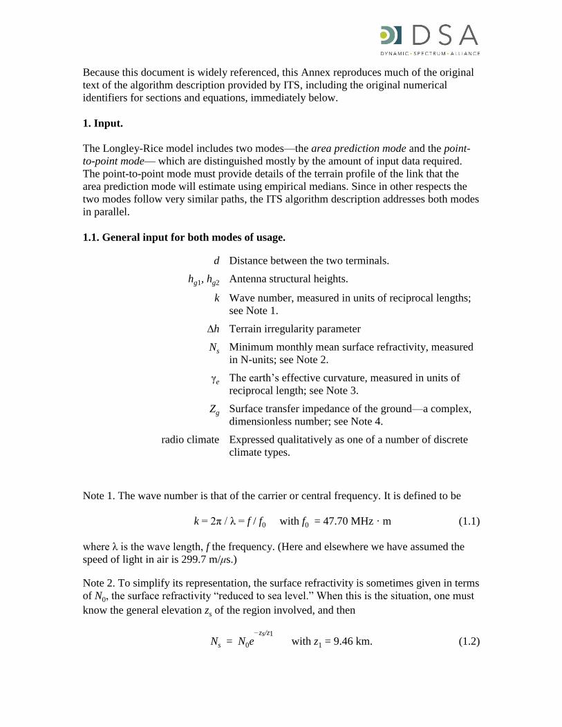
Note 1. The wave number is that of the carrier or central frequency. It is defined to be

k = 2π / λ = f / f0 with f0 = 47.70 MHz · m (1.1)

where λ is the wave length, f the frequency. (Here and elsewhere we have assumed the

speed of light in air is 299.7 m/μs.)

Note 2. To simplify its representation, the surface refractivity is sometimes given in terms

of N0, the surface refractivity “reduced to sea level.” When this is the situation, one must

know the general elevation zs of the region involved, and then

Ns = N0e−zs/z1 with z1 = 9.46 km. (1.2)

d Distance between the two terminals.

hg1, hg2 Antenna structural heights.

k Wave number, measured in units of reciprocal lengths;

see Note 1.

∆h Terrain irregularity parameter

Ns Minimum monthly mean surface refractivity, measured

in N-units; see Note 2.

γe

The earth’s effective curvature, measured in units of

reciprocal length; see Note 3.

Zg

Surface transfer impedance of the ground—a complex,

dimensionless number; see Note 4.

radio climate

Expressed qualitatively as one of a number of discrete

climate types.

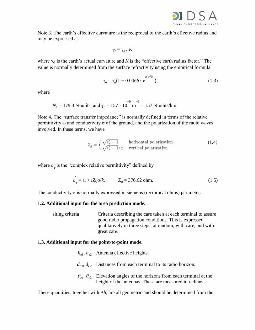
Note 3. The earth’s effective curvature is the reciprocal of the earth’s effective radius and

may be expressed as

γe = γa / K

where γa is the earth’s actual curvature and K is the “effective earth radius factor.” The

value is normally determined from the surface refractivity using the empirical formula

γe = γa(1 − 0.04665 eNs/N1 ) (1.3)

where

N1 = 179.3 N-units, and γa = 157 · 10−9

m−1

= 157 N-units/km.

Note 4. The “surface transfer impedance” is normally defined in terms of the relative

permittivity εr and conductivity σ of the ground, and the polarization of the radio waves

involved. In these terms, we have

where ε′r is the “complex relative permittivity” defined by

ε′r = εr + iZ0σ/k, Z0 = 376.62 ohm. (1.5)

The conductivity σ is normally expressed in siemens (reciprocal ohms) per meter.

1.2. Additional input for the area prediction mode.

siting criteria Criteria describing the care taken at each terminal to assure

good radio propagation conditions. This is expressed

qualitatively in three steps: at random, with care, and with

great care.

1.3. Additional input for the point-to-point mode.

he1, he2 Antenna effective heights.

dL1, dL2 Distances from each terminal to its radio horizon.

θe1, θe2 Elevation angles of the horizons from each terminal at the

height of the antennas. These are measured in radians.

These quantities, together with ∆h, are all geometric and should be determined from the

(1.4)

terrain profile that lies between the two terminals. We shall not go into detail here.

The “effective height” of an antenna is its height above an “effective reflecting plane” or

above the “intermediate foreground” between the antenna and its horizon. A difficulty

with the model is that there is no explicit definition of this quantity, and the accuracy of

the model sometimes depends on the skill of the user in estimating values for these

effective heights.

In the case of a line-of-sight path there are no horizons, but the model still requires values

for dLj, θej, j = 1,2. They should be determined from the formulas used in the area

prediction mode and listed in Section 3 below. Now it may happen that after these

computations one discovers d > dL = dL1 + dL2, implying that the path is a beyond-

horizon one. Noting that dL is a monotone increasing function of the hej we can assume

these latter have been underestimated and that they should be increased by a common

factor until dL = d.

2. Output.

The output from the model may take on one of several forms at the user’s option.

Simplest of these forms is just the reference attenuation Aref . This is the median

attenuation relative to a free space signal that should be observed on the set of all similar

paths during times when the atmospheric conditions correspond to a standard, well-

mixed, atmosphere.

The second form of output provides the two- or three-dimensional cumulative

distribution of attenuation in which time, location, and situation variability are all

accounted for. This is done by giving the quantile A(qT,qL,qS), the attenuation that will

not be exceeded as a function of the fractions of time, locations, and situations. One says

In qS of the situations there will be at least qL of the locations where the attenuation does

not exceed A(qT,qL,qS) for at least qT of the time.

When the point-to-point mode is used on particular, well-defined paths with definitely

fixed terminals, there is no location variability, and one must use a two-dimensional

description of cumulative distributions. One can now say With probability (or

confidence) qS the attenuation will not exceed A(qT, qS ) for at least qT of the time. The

same effect can be achieved by setting qL = 0.5 in the three-dimensional formulation.

On some occasions it will be desirable to go beyond the three-dimensional quantiles and

to treat directly the underlying model of variability. For example, consider the case of a

communications link that is to be used once and once only. For such a “one-shot” system

one is interested only in what probability or confidence an adequate signal is received

that once. The three-dimensional distributions used above must now be combined into

one.

3. Preparatory Calculations.

We start with some preliminary calculations of a geometric nature.

3.1. Preparatory calculations for the area prediction mode.

The parameters hej, dLj, θej, j = 1,2,which are part of the input in the point-to-point mode

are, in the area prediction mode, estimated using empirical formulas in which ∆h plays an

important role.

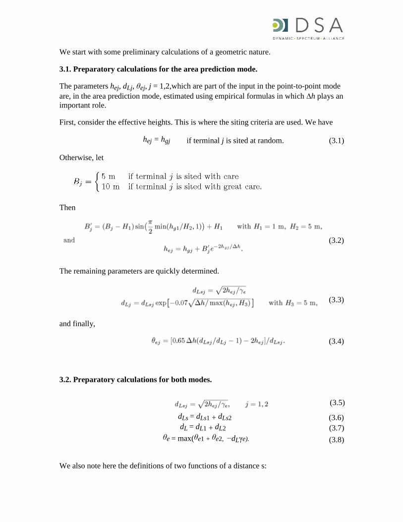
First, consider the effective heights. This is where the siting criteria are used. We have

hej = hgj if terminal j is sited at random. (3.1)

Otherwise, let

Then

The remaining parameters are quickly determined.

and finally,

3.2. Preparatory calculations for both modes.

dLs = dLs1 + dLs2 (3.6)

dL = dL1 + dL2 (3.7)

θe = max(θe1 + θe2, −dLγe). (3.8)

We also note here the definitions of two functions of a distance s:

(3.2)

(3.3)

(3.4)

(3.5)

and

4. The Reference Attenuation.

The reference attenuation is determined as a function of the distance d from the piecewise

formula

where the coefficients Ael, K1, K2, Aed, md, Aes, ms, and the distance dx are calculated

using the algorithms below. The three intervals defined here are called the line-of-sight,

diffraction, and scatter regions, respectively. The function in (4.1) is continuous so that at

the two endpoints where d = dLs or dx the two formulas give the same results. It follows

that instead of seven independent coefficients there are really only five.

4.1. Coefficients for the diffraction range.

Set

Xae = (kγ2e)

−1/3 (4.2)

d3 = max(dLs, dL + 1.3787 Xae) (4.3)

d4 = d3 + 2.7574 Xae (4.4)

A3 = Adiff(d3) (4.5)

A4 = Adiff(d4) (4.6)

where Adiff is the function defined below. The formula for Aref in the diffraction range is

then just the linear function having the values A3 and A4 at the distances d3 and d4,

respectively. Thus

md = (A4 − A3)/(d4 − d3) (4.7)

Aed = A3 − mdd3. (4.8)

4.1.1. The function Adiff(s).

We first define the weighting factor

(3.9)

(3.10)

(4.1)

with

and

and where ∆h(s) is the function defined in (3.9) above. Next we define a “clutter factor”

and with σh(s) defined in (3.10) above.

Then

Adiff(s) = (1 − w)Ak + wAr + Afo (4.11)

where the “double knife edge attenuation” Ak and the “rounded earth attenuation” Ar

are yet to be defined. Set

θ = θe + sγe (4.12)

and then

Ak = Fn(v1) + Fn(v2) (4.14)

where Fn(v) is the Fresnel integral defined below.

For the rounded earth attenuation we use a “three radii” method applied to Volger’s

formulation of the solution to the smooth, spherical earth problem. We set

γ0 = θ / (s – dL) γj = 2hej / d2Lj, j = 1,2 (4.15)

αj = (k/γj)1/3, j = 0,1,2 (4.16)

(4.9)

(4.10)

(4.13)

Note that the Kj are complex numbers. To continue, we set

xj = AB(Kj)αjγjdLj, j = 1.2 (4.18)

x0 = AB(K0)α0θ + x1 + x2 (4.19)

and then

Ar = G(x0) – F (x1, K1) – F (x2, K2) – C1(K0) (4.20)

where A = 151.03 is a dimensionless constant and the functions B(K), G(x), F (x, K), and

C1(K) are those defined by Vogler.

In (4.14) and (4.20) we have finished the definition of Adiff. We should like, however, to

complete the subject by defining more precisely the more or less standard functions

mentioned above. The Fresnel integral, for example, may be written as

For Vogler’s formulation to the solution to the spherical earth problem, we first introduce

the special Airy function

Wi(z) = Ai(z) + iBi(z)

= 2Ai(e2πi/3z)

where Ai(z) and Bi(z) are the two standard Airy functions defined in many texts. They are

analytic in the entire complex plane and are particular solutions to the differential

equation

w”

(z) − zw(z) = 0.

First, to define the function B(K) we find the smallest solution to the modal equation

Wi(t0) = 21/3

KWi′(t0)

and then

B = 2−1/3

Im{t0}. (4.22)

Finally, we also have

(4.17)

(4.21)

where A is again the constant defined above.

It is of interest to note that for large x we find F (x, K ) ~ G(x), and that for those values

of K in which we are interested it is a good approximation to say C1(K) = 20 dB.

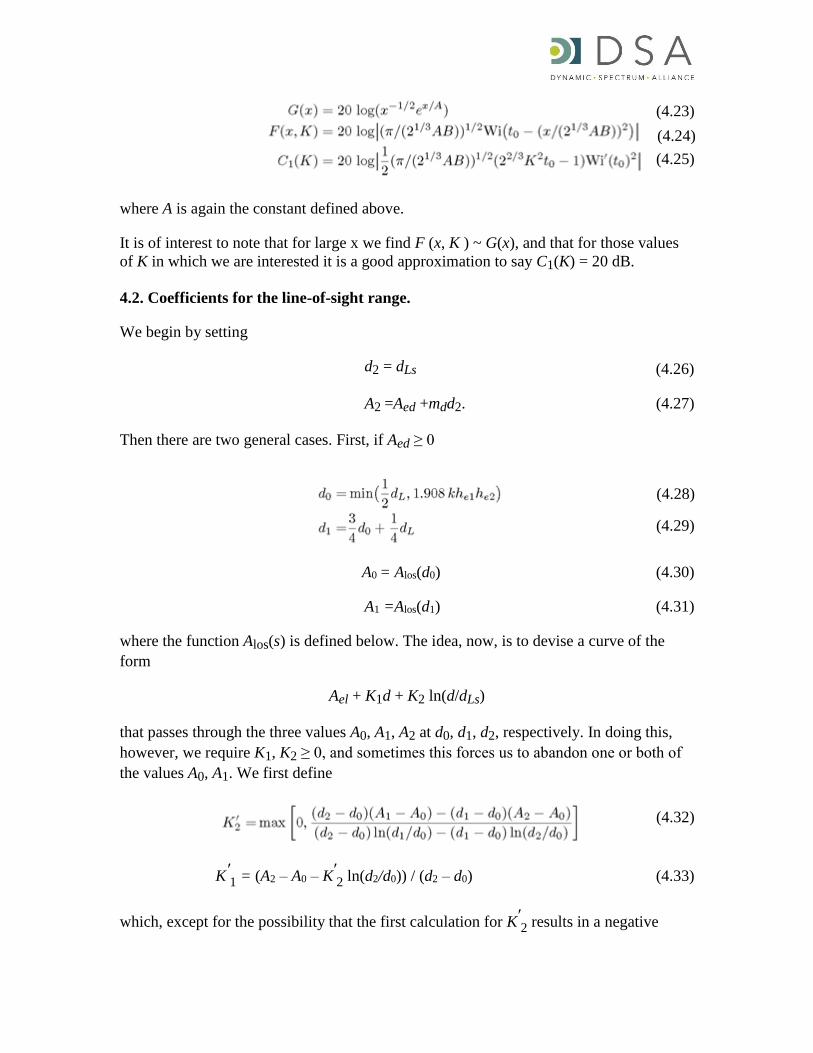
4.2. Coefficients for the line-of-sight range.

We begin by setting

d2 = dLs (4.26)

A2 =Aed +mdd2. (4.27)

Then there are two general cases. First, if Aed ≥ 0

A0 = Alos(d0) (4.30)

A1 =Alos(d1) (4.31)

where the function Alos(s) is defined below. The idea, now, is to devise a curve of the

form

Ael + K1d + K2 ln(d/dLs)

that passes through the three values A0, A1, A2 at d0, d1, d2, respectively. In doing this,

however, we require K1, K2 ≥ 0, and sometimes this forces us to abandon one or both of

the values A0, A1. We first define

K′1 = (A2 – A0 – K′

2 ln(d2/d0)) / (d2 – d0) (4.33)

which, except for the possibility that the first calculation for K′2 results in a negative

(4.23)

(4.24)

(4.25)

(4.28)

(4.29)

(4.32)

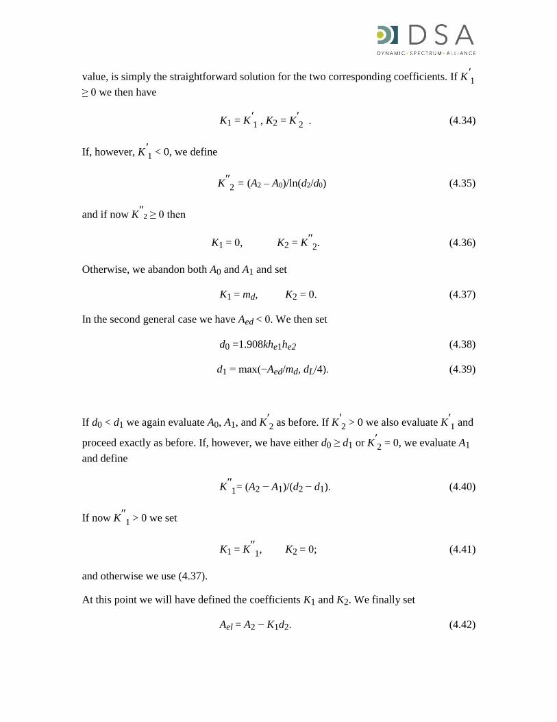
value, is simply the straightforward solution for the two corresponding coefficients. If K′1

≥ 0 we then have

K1 = K′1 , K2 = K′

2 . (4.34)

If, however, K′1 < 0, we define

K′′2 = (A2 – A0)/ln(d2/d0) (4.35)

and if now K′′2 ≥ 0 then

K1 = 0, K2 = K′′2. (4.36)

Otherwise, we abandon both A0 and A1 and set

K1 = md, K2 = 0. (4.37)

In the second general case we have Aed < 0. We then set

d0 =1.908khe1he2 (4.38)

d1 = max(−Aed/md, dL/4). (4.39)

If d0 < d1 we again evaluate A0, A1, and K′2 as before. If K′

2 > 0 we also evaluate K′

1 and

proceed exactly as before. If, however, we have either d0 ≥ d1 or K′2 = 0, we evaluate A1

and define

K′′1= (A2 − A1)/(d2 − d1). (4.40)

If now K′′1 > 0 we set

K1 = K′′1, K2 = 0; (4.41)

and otherwise we use (4.37).

At this point we will have defined the coefficients K1 and K2. We finally set

Ael = A2 − K1d2. (4.42)

4.2.1. The function Alos(s).

First we define the weighting factor

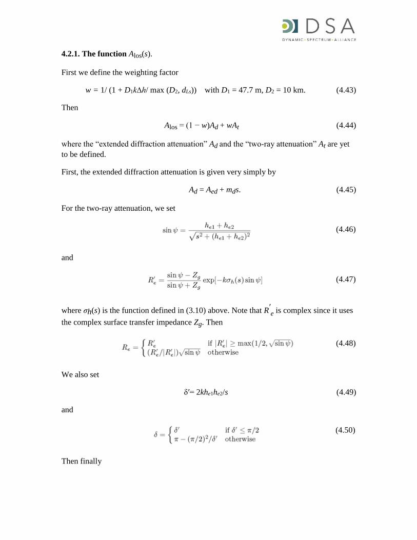
w = 1/ (1 + D1k∆h/ max (D2, dLs)) with D1 = 47.7 m, D2 = 10 km. (4.43)

Then

Alos = (1 − w)Ad + wAt (4.44)

where the “extended diffraction attenuation” Ad and the “two-ray attenuation” At are yet

to be defined.

First, the extended diffraction attenuation is given very simply by

Ad = Aed + mds. (4.45)

For the two-ray attenuation, we set

and

where σh(s) is the function defined in (3.10) above. Note that R′e is complex since it uses

the complex surface transfer impedance Zg. Then

We also set

δʹ= 2khe1he2/s (4.49)

and

Then finally

(4.46)

(4.47)

(4.48)

(4.50)

4.3. Coefficients for the scatter range.

Set

d5 =dL + Ds (4.52)

d6 =d5 + Ds with Ds = 200 km. (4.53)

Then define

A5 =Ascat(d5) (4.54)

A6 =Ascat(d6), (4.55)

where Ascat(s) is defined below. There are, however, some sets of parameters for which

Ascat is not defined, and it may happen that either or both A5, A6 is undefined. If this is so,

one merely sets

dx = +∞ (4.56)

and one can let Aes, ms remain undefined. In the more normal situation one has

ms = (A6 – A5)/Ds (4.57)

dx = max[dLs, dL + Xae log(kHs), (A5 – Aed – msd5)/(md – ms)] (4.58)

Aes = Aed + (md – ms)dx (4.59)

where Ds is the distance given above, where Xae has been defined in (4.2), and where

Hs= 47.7 m.

4.3.1. The function Ascat.

Computation of this function uses an abbreviated version of the methods described in

Section 9 and Annex III.5 of NBS TN101.7 First, set

θ =θe + γes (4.60)

θʹ =θe1 + θe2 + γes (4.61)

rj =2kθʹhej, j = 1,2. (4.62)

7 See P. L. Rice, A. G. Longley, K. A. Norton, and A. P. Barsis, “Transmission loss predictions for

tropospheric communication circuits,” U.S. Government Printing Office, Washington, DC, NBS Tech.

Note 101, issued May 1965; revised May 1966 and Jan. 1967 (“TN101”).

(4.51)

If both r1 and r2 are less than 0.2 the function Ascat is not defined (or is infinite).

Otherwise we put

Ascat (s) = 10 log(kHθ4) + F(θs, Ns) + H0 (4.63)

where F (θs, Ns) is the function shown in Figure 9.1 of TN101, H0 is the “frequency gain

function”, and H = 47.7m.

The frequency gain function H0 is a function of r1, r2, the scatter efficiency factor ηs, and

the “asymmetry factor” which we shall here call ss. A difficulty with the present model is

that there is not sufficient geometric data in the input variables to determine where the

crossover point is. This is resolved by assuming it to be midway between the two

horizons. The asymmetry factor, for example, is found by first defining the distance

between horizons

ds = s – dL1 – dL2 (4.64)

whereupon

There then follows that the height of the crossover point is

and then

where

Z0 =1.756 km Z1 =8.0 km

The computation of H0 then proceeds according to the rules in Section 9.3 and Figure 9.3

of TN101.

The model requires these results at the two distances s = d5, d6, described above. One

further precaution is taken to prevent anomalous results. If, at d5, calculations show that

H0 will exceed 15 dB, they are replaced by the value it has at d6. This helps keep the

scatter-mode slope within reasonable bounds.

(4.65)

(4.66)

(4.67)

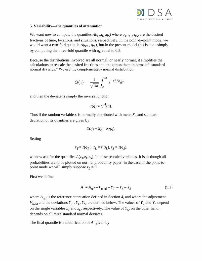
5. Variability—the quantiles of attenuation.

We want now to compute the quantiles A(qT,qL,qS) where qT, qL, qS, are the desired

fractions of time, locations, and situations, respectively. In the point-to-point mode, we

would want a two-fold quantile A(qT , qS ), but in the present model this is done simply

by computing the three-fold quantile with qL equal to 0.5.

Because the distributions involved are all normal, or nearly normal, it simplifies the

calculations to rescale the desired fractions and to express them in terms of “standard

normal deviates.” We use the complementary normal distribution

and then the deviate is simply the inverse function

z(q) = Q-1

(q).

Thus if the random variable x is normally distributed with mean X0 and standard

deviation σ, its quantiles are given by

X(q) = X0 + σz(q).

Setting

zT = z(qT ), zL = z(qL), zS = z(qS),

we now ask for the quantiles A(zT,zL,zS). In these rescaled variables, it is as though all

probabilities are to be plotted on normal probability paper. In the case of the point-to-

point mode we will simply suppose zL = 0.

First we define

A’

= Aref – Vmed – YT – YL – YS (5.1)

where Aref is the reference attenuation defined in Section 4, and where the adjustment

Vmed and the deviations YT , YL, YS, are defined below. The values of YT and YL depend

on the single variables zT and zL, respectively. The value of YS, on the other hand,

depends on all three standard normal deviates.

The final quantile is a modification of A’ given by

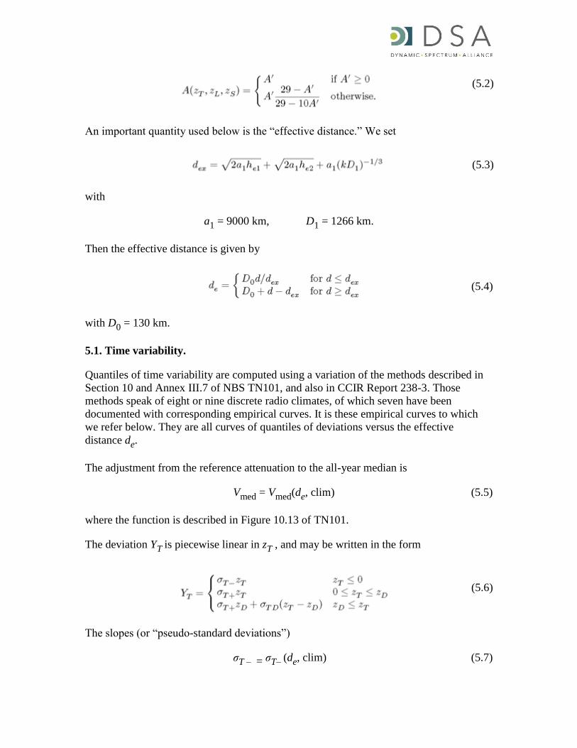
An important quantity used below is the “effective distance.” We set

with

a1 = 9000 km, D1 = 1266 km.

Then the effective distance is given by

with D0 = 130 km.

5.1. Time variability.

Quantiles of time variability are computed using a variation of the methods described in

Section 10 and Annex III.7 of NBS TN101, and also in CCIR Report 238-3. Those

methods speak of eight or nine discrete radio climates, of which seven have been

documented with corresponding empirical curves. It is these empirical curves to which

we refer below. They are all curves of quantiles of deviations versus the effective

distance de.

The adjustment from the reference attenuation to the all-year median is

Vmed = Vmed(de, clim) (5.5)

where the function is described in Figure 10.13 of TN101.

The deviation YT is piecewise linear in zT , and may be written in the form

The slopes (or “pseudo-standard deviations”)

σT – = σT– (de, clim) (5.7)

(5.2)

(5.3)

(5.4)

(5.6)

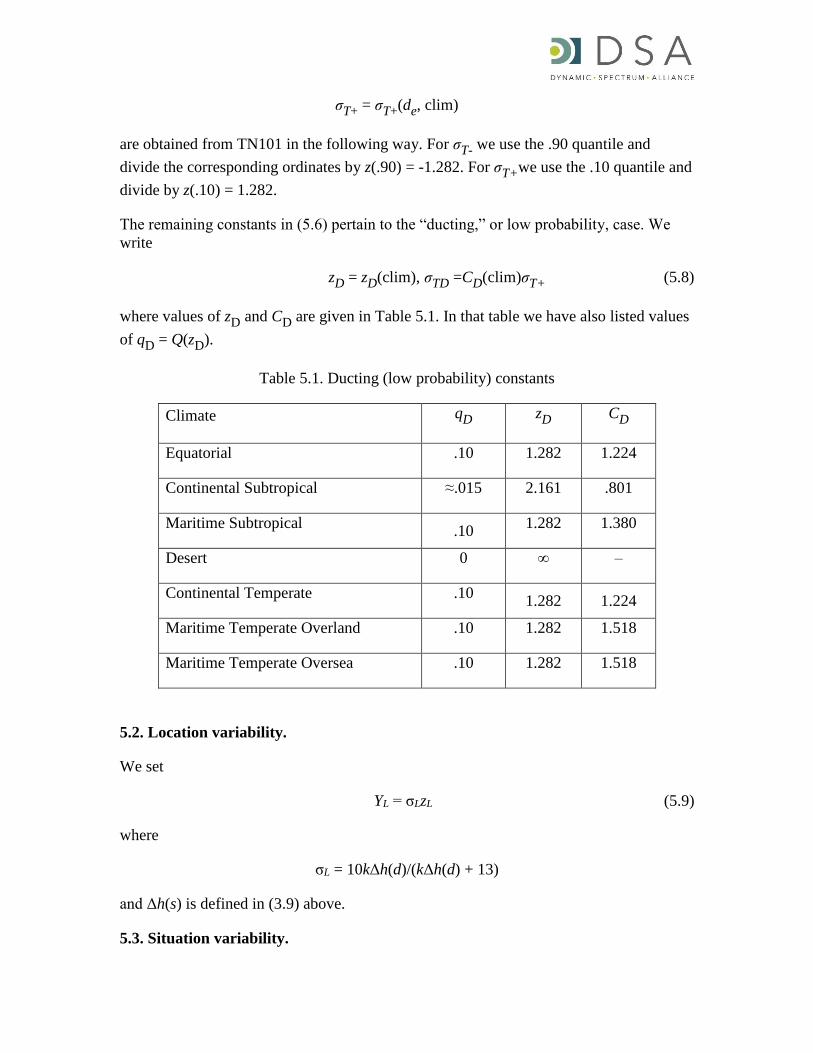
σT+ = σT+(de, clim)

are obtained from TN101 in the following way. For σT- we use the .90 quantile and

divide the corresponding ordinates by z(.90) = -1.282. For σT+we use the .10 quantile and

divide by z(.10) = 1.282.

The remaining constants in (5.6) pertain to the “ducting,” or low probability, case. We

write

zD = zD(clim), σTD =CD(clim)σT+ (5.8)

where values of zD and CD are given in Table 5.1. In that table we have also listed values

of qD = Q(zD).

Table 5.1. Ducting (low probability) constants

Climate qD zD CD

Equatorial .10 1.282 1.224

Continental Subtropical ≈.015 2.161 .801

Maritime Subtropical .10

1.282 1.380

Desert 0 ∞ –

Continental Temperate .10 1.282 1.224

Maritime Temperate Overland .10 1.282 1.518

Maritime Temperate Oversea .10 1.282 1.518

5.2. Location variability.

We set

YL = σLzL (5.9)

where

σL = 10kΔh(d)/(kΔh(d) + 13)

and Δh(s) is defined in (3.9) above.

5.3. Situation variability.

Set

σS = 5 + 3e – de/D (5.10)

where D = 100 km. Then

The latter is intended to reveal how the uncertainties become greater in the wings of the

distributions.

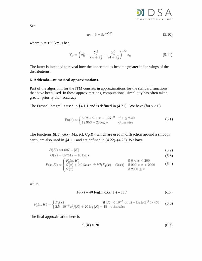
6. Addenda—numerical approximations.

Part of the algorithm for the ITM consists in approximations for the standard functions

that have been used. In these approximations, computational simplicity has often taken

greater priority than accuracy.

The Fresnel integral is used in §4.1.1 and is defined in (4.21). We have (for v > 0)

The functions B(K), G(x), F(x, K), C1(K), which are used in diffraction around a smooth

earth, are also used in §4.1.1 and are defined in (4.22)–(4.25). We have

where

F1(x) = 40 log(max(x, 1)) – 117 (6.5)

The final approximation here is

C1(K) ≈ 20 (6.7)

(5.11)

(6.1)

(6.6)

(6.2)

(6.3)

(6.4)

To complete this section we have the two functions, F(θd) and H0, used for tropospheric

scatter. First,

F(D, Ns) = F0(D) – 0.1(Ns – 301)e – D/D0 (6.8)

where

D0 = 40 km

and (when D is given in meters)

The frequency gain function may be written as

H0 = H00 (r1, r2, ηs) + ∆H0 (6.10)

where

∆H0 = 6(0.6 – logηs) log ss log r2/ ss r1 (6.11)

and where H00 is obtained by linear interpolation between its values when ηs is an

integer. For ηs = 1, ... ,5 we set

with

For ηs > 5 we use the value for ηs = 5 and for ηs = 0 we suppose

In all of this, we truncate the values of ss and q = r2/ssr1 at 0.1 and 10.

(6.14)

(6.13)

(6.12)

(6.9)

Annex B: Longley-Rice Parameters for TV Broadcast Field Strength Calculations

I. Introduction

Annex B provides a description of elements to be taken into account in implementing the

Longley-Rice radio propagation model—also known as the Irregular Terrain Model

(“ITM”)—in order to use this model to calculate the field strength of a television

broadcasting station signal at a particular geographic location. As described in Annex A,

implementations of the Longley-Rice model occur as programs written in a specific

computer language. For example, the Institute for Telecommunication Sciences (“ITS”),

a research and engineering laboratory of the National Telecommunications and

Information Administration (“NTIA”) within the United States Department of

Commerce, maintains the “definitive” representation of the Longley-Rice model, which

is written in FORTRAN.1

These software implementations of the Longley-Rice radio propagation model will

require several inputs to perform the field strength calculation for broadcast television.

Although the specific inputs may depend on the particular software implementation used

or developed, required parameters/data generally will fall into four categories:

a. Television Broadcasting Station Parameters

b. Planning Factors for Television Reception

c. Longley-Rice Environmental Parameters

d. Terrain Profile Data

In addition, certain path calculations—described below—will need to be taken into

account in order to predict television broadcasting field strength at a given location.

II. Model Parameters

The Longley-Rice radio propagation model can be implemented in “area” mode or

“point-to-point” mode. The point-to-point mode is used to evaluate the predicted

strength of a particular television channel at a geographic location where a White Space

Device (“WSD”) is present. With the point-to-point mode, field strength at a particular

geographic location is determined using path-specific parameters determined from

detailed terrain profile data. In addition to the location of the WSD and the WSD antenna

height (for fixed WSD deployments), software implementations of the Longley-Rice

model will require the following input parameters.

1 See generally Implementation of the Irregular Terrain Model, version 1.2.2 (updated 5 Aug. 2002),

available at http://www.its.bldrdoc.gov/media/35869/itm.pdf.

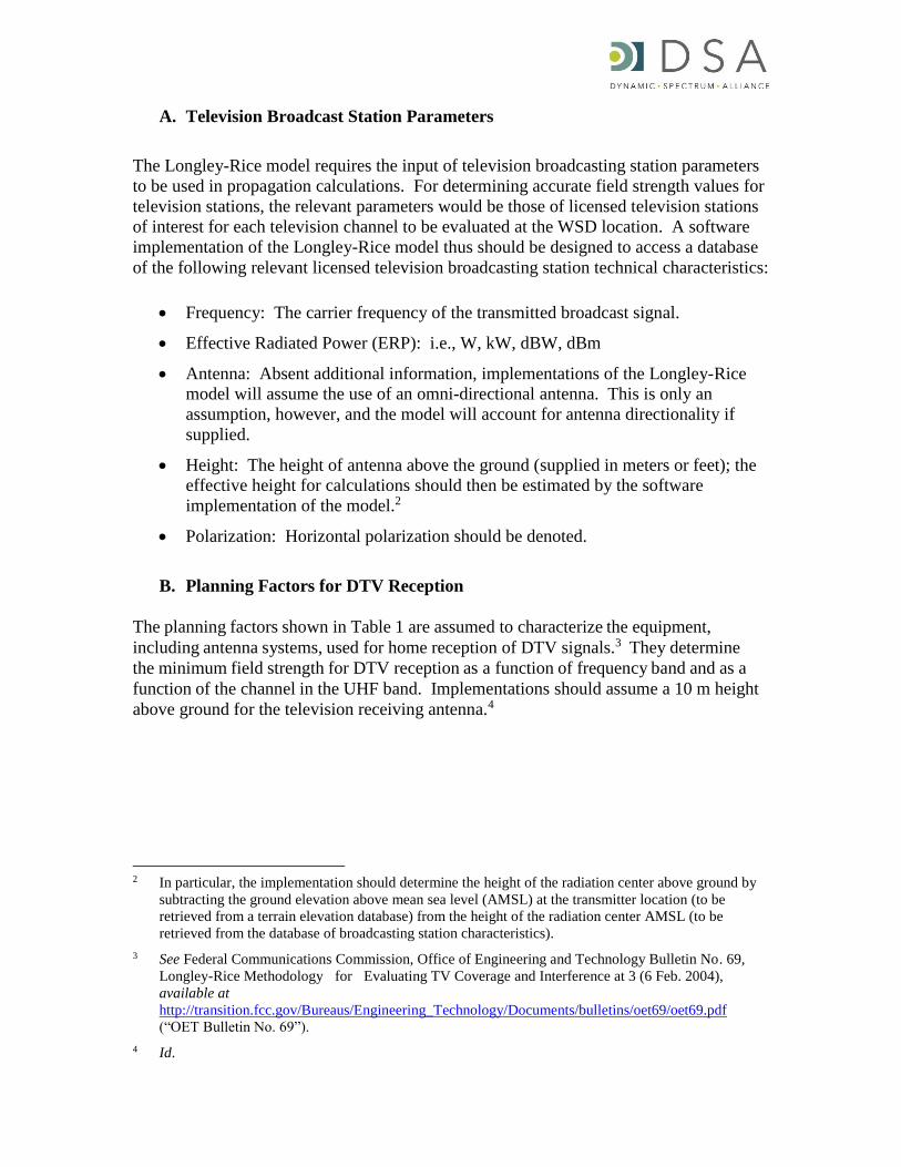
A. Television Broadcast Station Parameters

The Longley-Rice model requires the input of television broadcasting station parameters

to be used in propagation calculations. For determining accurate field strength values for

television stations, the relevant parameters would be those of licensed television stations

of interest for each television channel to be evaluated at the WSD location. A software

implementation of the Longley-Rice model thus should be designed to access a database

of the following relevant licensed television broadcasting station technical characteristics:

Frequency: The carrier frequency of the transmitted broadcast signal.

Effective Radiated Power (ERP): i.e., W, kW, dBW, dBm

Antenna: Absent additional information, implementations of the Longley-Rice

model will assume the use of an omni-directional antenna. This is only an

assumption, however, and the model will account for antenna directionality if

supplied.

Height: The height of antenna above the ground (supplied in meters or feet); the

effective height for calculations should then be estimated by the software

implementation of the model.2

Polarization: Horizontal polarization should be denoted.

B. Planning Factors for DTV Reception

The planning factors shown in Table 1 are assumed to characterize the equipment,

including antenna systems, used for home reception of DTV signals.3 They determine

the minimum field strength for DTV reception as a function of frequency band and as a

function of the channel in the UHF band. Implementations should assume a 10 m height

above ground for the television receiving antenna.4

2 In particular, the implementation should determine the height of the radiation center above ground by

subtracting the ground elevation above mean sea level (AMSL) at the transmitter location (to be

retrieved from a terrain elevation database) from the height of the radiation center AMSL (to be

retrieved from the database of broadcasting station characteristics).

3 See Federal Communications Commission, Office of Engineering and Technology Bulletin No. 69,

Longley-Rice Methodology for Evaluating TV Coverage and Interference at 3 (6 Feb. 2004),

available at

http://transition.fcc.gov/Bureaus/Engineering_Technology/Documents/bulletins/oet69/oet69.pdf

(“OET Bulletin No. 69”).

4 Id.

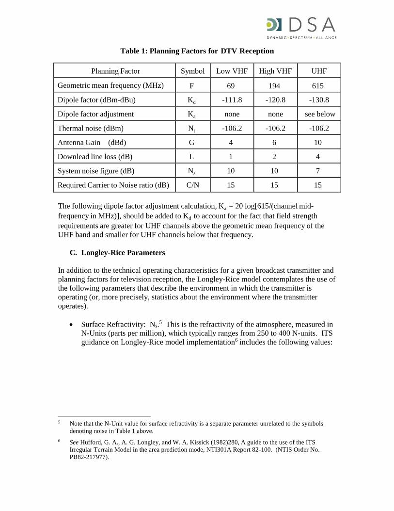
Table 1: Planning Factors for DTV Reception

Planning Factor

Symbol

Low VHF

High VHF

UHF

Geometric mean frequency (MHz)

F

69

194

615

Dipole factor (dBm-dBu) Kd -111.8 -120.8 -130.8

Dipole factor adjustment Ka none none see below

Thermal noise (dBm) Nt -106.2 -106.2 -106.2

Antenna Gain (dBd) G 4 6 10

Downlead line loss (dB) L 1 2 4

System noise figure (dB) Ns 10 10 7

Required Carrier to Noise ratio (dB) C/N 15 15 15

The following dipole factor adjustment calculation, Ka = 20 log[615/(channel mid-

frequency in MHz)], should be added to Kd to account for the fact that field strength

requirements are greater for UHF channels above the geometric mean frequency of the

UHF band and smaller for UHF channels below that frequency.

C. Longley-Rice Parameters

In addition to the technical operating characteristics for a given broadcast transmitter and

planning factors for television reception, the Longley-Rice model contemplates the use of

the following parameters that describe the environment in which the transmitter is

operating (or, more precisely, statistics about the environment where the transmitter

operates).

Surface Refractivity: Ns.5 This is the refractivity of the atmosphere, measured in

N-Units (parts per million), which typically ranges from 250 to 400 N-units. ITS

guidance on Longley-Rice model implementation6 includes the following values:

5 Note that the N-Unit value for surface refractivity is a separate parameter unrelated to the symbols

denoting noise in Table 1 above.

6 See Hufford, G. A., A. G. Longley, and W. A. Kissick (1982)280, A guide to the use of the ITS

Irregular Terrain Model in the area prediction mode, NTI301A Report 82-100. (NTIS Order No.

PB82-217977).

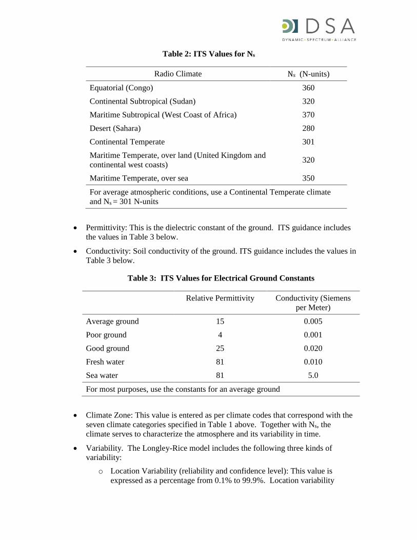
Table 2: ITS Values for Ns

Radio Climate Ns (N-units)

Equatorial (Congo) 360

Continental Subtropical (Sudan) 320

Maritime Subtropical (West Coast of Africa) 370

Desert (Sahara) 280

Continental Temperate 301

Maritime Temperate, over land (United Kingdom and

continental west coasts) 320

Maritime Temperate, over sea 350

For average atmospheric conditions, use a Continental Temperate climate

and Ns = 301 N-units

Permittivity: This is the dielectric constant of the ground. ITS guidance includes

the values in Table 3 below.

Conductivity: Soil conductivity of the ground. ITS guidance includes the values in

Table 3 below.

Table 3: ITS Values for Electrical Ground Constants

Climate Zone: This value is entered as per climate codes that correspond with the

seven climate categories specified in Table 1 above. Together with Ns, the

climate serves to characterize the atmosphere and its variability in time.

Variability. The Longley-Rice model includes the following three kinds of

variability:

o Location Variability (reliability and confidence level): This value is

expressed as a percentage from 0.1% to 99.9%. Location variability

Relative Permittivity Conductivity (Siemens

per Meter)

Average ground 15 0.005

Poor ground 4 0.001

Good ground 25 0.020

Fresh water 81 0.010

Sea water 81 5.0

For most purposes, use the constants for an average ground

accounts for variations in long-term statistics that occur from path to path.

o Time Variability: This value is expressed as percentage from 0 to 100%.

Time variability accounts for variations of median values of attenuation.

o Situation Variability: This value is expressed as a percentage; 50%

variability is considered normal for coverage estimations. Situation

variability accounts for variations between systems with the same system

parameters and environmental conditions.

Variability modes: ITS guidance contemplates the following ways in which the

kinds of variability listed above are treated in combination:

o Broadcast mode: all three kinds of variability are treated separately.

o Individual mode: situation and location variability are combined; time

variability is treated separately.

o Mobile mode: time and location variability are combined; situation

variability is treated separately.

o Single message mode: all three kinds of variability are combined.

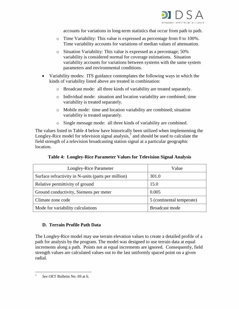
The values listed in Table 4 below have historically been utilized when implementing the

Longley-Rice model for television signal analysis,7 and should be used to calculate the

field strength of a television broadcasting station signal at a particular geographic

location.

Table 4: Longley-Rice Parameter Values for Television Signal Analysis

Longley-Rice Parameter Value

Surface refractivity in N-units (parts per million) 301.0

Relative permittivity of ground 15.0

Ground conductivity, Siemens per meter 0.005

Climate zone code 5 (continental temperate)

Mode for variability calculations Broadcast mode

D. Terrain Profile Path Data

The Longley-Rice model may use terrain elevation values to create a detailed profile of a

path for analysis by the program. The model was designed to use terrain data at equal

increments along a path. Points not at equal increments are ignored. Consequently, field

strength values are calculated values out to the last uniformly spaced point on a given

radial.

7 See OET Bulletin No. 69 at 6.

A Longley-Rice implementation may achieve greater precision by utilizing values given

by specific terrain datasets collected using empirical measurements. For example, the

Shuttle Radar Topography Mission (SRTM) undertaken by the National Aeronautics and

Space Administration (NASA) obtained elevation data on a near-global scale in order to

create a high-resolution digital topographic database of most of the Earth, providing 3

arc-second (~ 90 m) resolution data for most of the continents between 60 N and 60 S.8

In many populated areas, higher resolution sources of terrain data are available.

III. Path Calculations

The Longley-Rice model uses input parameters to compute geometric parameters related

to the propagation path. First, the model determines effective antenna height. Since this is

an area prediction model, the radio horizons, for example, are unknown. The model uses

the terrain irregularity parameter to estimate radio horizons. The model also computes a

reference attenuation, using horizon distances and elevation angles to calculate

transmission loss relative to free space.

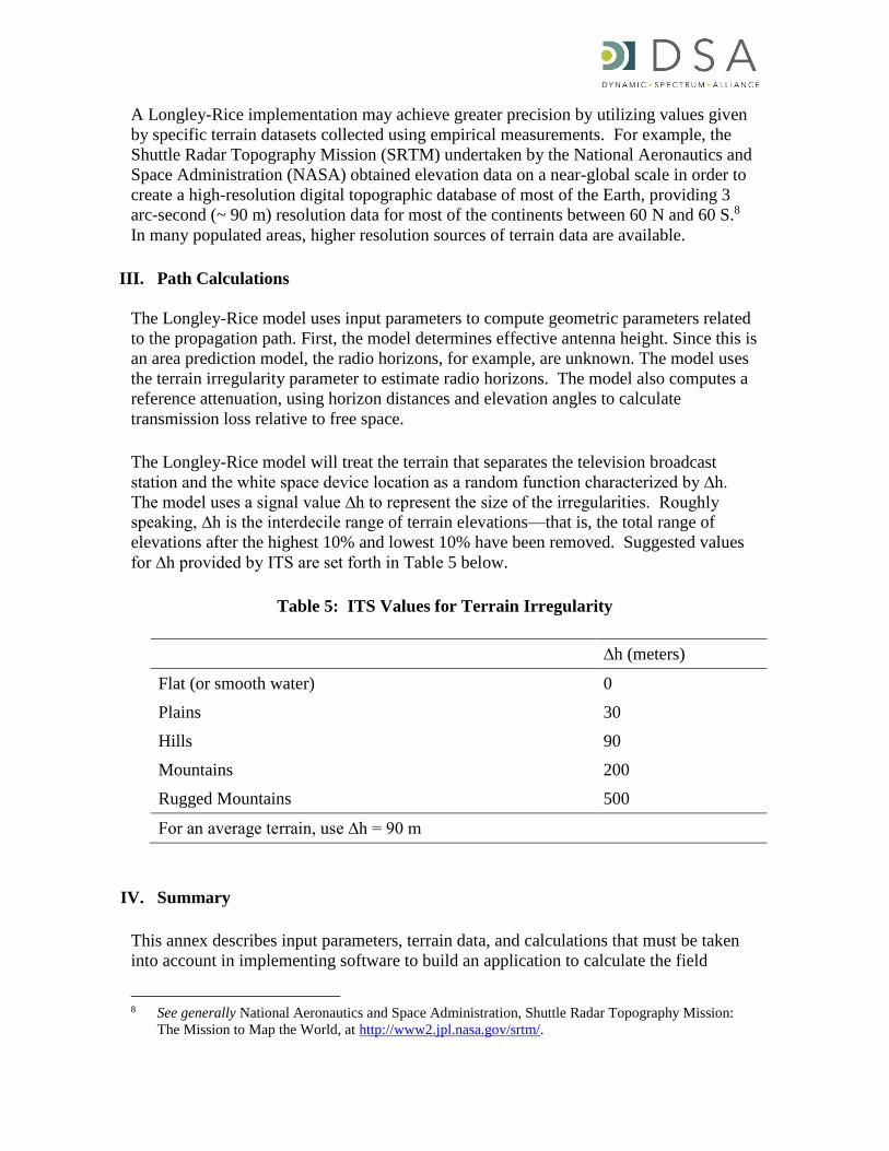
The Longley-Rice model will treat the terrain that separates the television broadcast

station and the white space device location as a random function characterized by ∆h.

The model uses a signal value ∆h to represent the size of the irregularities. Roughly

speaking, ∆h is the interdecile range of terrain elevations—that is, the total range of

elevations after the highest 10% and lowest 10% have been removed. Suggested values

for ∆h provided by ITS are set forth in Table 5 below.

Table 5: ITS Values for Terrain Irregularity

∆h (meters)

Flat (or smooth water) 0

Plains 30

Hills 90

Mountains 200

Rugged Mountains 500

For an average terrain, use ∆h = 90 m

IV. Summary

This annex describes input parameters, terrain data, and calculations that must be taken

into account in implementing software to build an application to calculate the field

8 See generally National Aeronautics and Space Administration, Shuttle Radar Topography Mission:

The Mission to Map the World, at http://www2.jpl.nasa.gov/srtm/.

strength of a television broadcasting station at a particular location. Determining the field

strength of relevant television broadcast stations at a specific location will be used to

determine at what level and at what power level a WSD may operate at that location

pursuant to the procedure outlined in Annex C.

Annex C: Calculation of Available TV White Space Frequencies and Power Limits

I. Introduction

This Annex provides the detailed parameters and methodology to calculate the frequencies and

maximum power limits for White Space Devices in such as way as to limit the probability of

harmful interference to other services to acceptable levels. The proposed methodology in this

Annex is independent of the radio propagation models that might be used in the calculations

described herein. However, it is imperative that point-to-point path-specific statistical radio

propagation models that are capable of utilizing digital terrain/elevation models must be used.

II. Definitions

This section describes the various entities and their relationships with regard to frequency and

signal strength calculations. Interference from White Space Devices (WSDs) is controlled by

limiting their radiated power. The following definitions describe an approach for how those

power limits can be calculated.

1. Protected services

1.1. Analog terrestrial television(ATT): PAL-I standard

The service area of an analog TV broadcast includes any locations where the signal to

noise ratio of its signal is greater than or equal to 17.0 dB plus a link margin of 13 dB.1

1 A service’s signal to noise ratio (SNR) limit is the minimum theoretical operating level for a

service to be functional, while the link margin accounts for the extra signal power that is

typically required to cope with real-world environments. The link margin provides a buffer so

that the service is somewhat robust against common signal impairments like multi-path, fading,

and interference.

Figure 1: Example coverage map showing “in service” areas extending out to blue areas,

purple = “too weak” (“out of service”)

1.2. Digital terrestrial television (DTT): DVB-T2 standard

The service area of a digital TV broadcast includes any locations where the signal to

noise ratio of its signal is greater than or equal to 17.0 dB plus a link margin of 13 dB.

Given that the proposed methodology analyzes transmitters individually, Single

Frequency Networks (SFNs) and Multi-Frequency Networks (MFNs) can be treated

similarly.

1.3. Radio astronomy sites (RASs)

The protected area of radio astronomy sites (RASs) particularly the Square Kilometer

Array (SKA) project sites are designated as Radio Quite Zones (RQZs). However, this

designation also extends to some other SKA sites that are not located within the RQZs.

The prescribed maximum received Power Spectral Density (PSD) at each site must be not

exceed -130 dBm/8MHz2. The methodology for calculating the necessary protection

2 Radio astronomy sensitivity based on ITU-R RA.769-2.

from White Space Devices is still to be determined and may not be required or applicable

in all jurisdictions.

1.4. Other:

Radio astronomy frequencies, lower band edge, upper band edge, wireless

microphones/program-making and special events equipment, studio-to-transmitter links,

cable TV receive sites and gap filter terrestrial television stations may require additional

protection. Further analysis and industry consultation is required. Again, with the

exception of upper and lower band edge users, these incumbents may not be present in all

jurisdictions.

2. Receiver characteristics

2.1. Analog television (PAL-I)

An analog TV receiver’s sensitivity to White Space Device interference is a function of

its adjacent channel rejection ratio (ACR). If a receiver is tuned to channel “N”, it can

tolerate signals on adjacent channels without harmful interference if the relative signal

strength are less than the values given in Table 1.3

Table 1: Analog TV adjacent channel rejection ratios

Channel offset

Relative signal strength

(dB)

N-10 or lower 62

N-9 60

N-8 58

N-4 55

N-3 45

N-2 42

N-1 36

N+1 36

3 The ACR performance values are based on an Ofcom analysis of 50 commercially available

receivers currently on the market. See Ofcom, TV White Spaces: Approach to Coexistence,

Technical Analysis, Sept. 4, 2013, available at

http://stakeholders.ofcom.org.uk/binaries/consultations/white-space-

coexistence/annexes/technical-report.pdf (Ofcom Technical Report).

N+2 42

N+3 45

N+4 55

N+84 58

N+9 475

N+10 or higher 62

4 Values between N±4 and N±8 should be linearly interpolated. 5 The ACR performance on channel N+9 is different than N-9 due to internal tuner design

limitations.

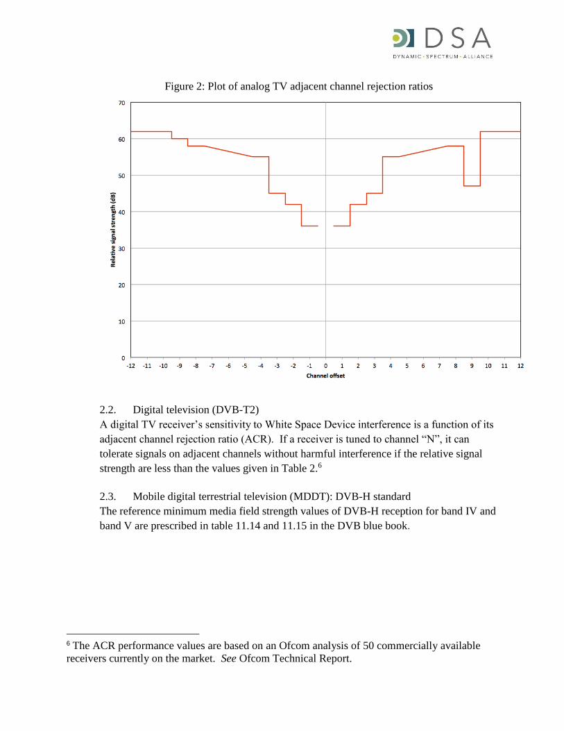
Figure 2: Plot of analog TV adjacent channel rejection ratios

2.2. Digital television (DVB-T2)

A digital TV receiver’s sensitivity to White Space Device interference is a function of its

adjacent channel rejection ratio (ACR). If a receiver is tuned to channel “N”, it can

tolerate signals on adjacent channels without harmful interference if the relative signal

strength are less than the values given in Table 2.6

2.3. Mobile digital terrestrial television (MDDT): DVB-H standard

The reference minimum media field strength values of DVB-H reception for band IV and

band V are prescribed in table 11.14 and 11.15 in the DVB blue book.

6 The ACR performance values are based on an Ofcom analysis of 50 commercially available

receivers currently on the market. See Ofcom Technical Report.

Table 2: Digital TV adjacent channel rejection ratios

Channel offset

Relative signal strength

(dB)

N-10 or lower 62

N-9 60

N-8 58

N-4 55

N-3 45

N-2 42

N-1 36

N+1 36

N+2 42

N+3 45

N+4 55

N+87 58

N+9 478

N+10 or higher 62

7 Values between N±4 and N±8 should be linearly interpolated. 8 The ACS performance on channel N+9 is different than N-9 due to internal tuner design

limitations.

Figure 3: Plot of digital TV adjacent channel rejection ratios

3. WSD coupling loss

The coupling loss between a White Space Device and other types of receivers is assumed

to be 60 dB.9

4. Resolving Terrain Overlap

Terrain data files are generally organized in “tiles” (rectangular rasters aligned to latitude

and longitude bins) that include overlapping data along each of its edges. When

overlapping tiles contain non-identical data in their overlapping zones, there is the

potential for elevation ambiguity in those areas.

To resolve this ambiguity, the following tile selection methodology shall be used. For

any given point, exactly one terrain tile will be selected as the authoritative source of

9 The coupling loss accounts for a multitude of factors, including the separation distance between

devices, antenna discrimination, polarization discrimination, building attenuation, physical

obstructions, etc.

elevation data.

1. For any given point (lat and lon), determine the set of tiles that include the

requested lat and lon coordinates. The number of matching tile candidates is

expected to be between 0 and 4.

a. If the number of matching tiles is 0 (point does not fall within any

terrain tile), then treat the elevation as 0 meters and return.

b. If the number of matching tiles is 1, then the point does not have any

data overlap issues. Use bilinear interpolation to compute the terrain

elevation using the selected tile.

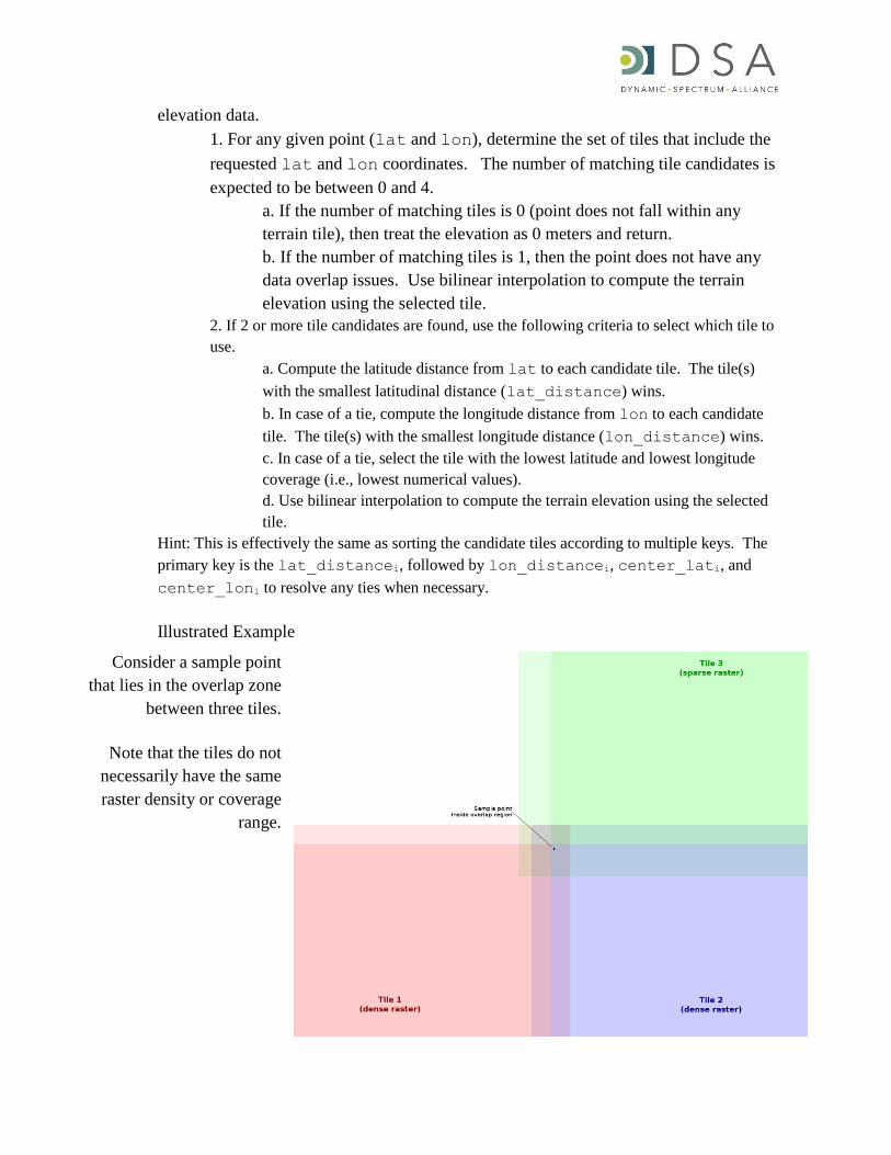
2. If 2 or more tile candidates are found, use the following criteria to select which tile to

use.

a. Compute the latitude distance from lat to each candidate tile. The tile(s)

with the smallest latitudinal distance (lat_distance) wins.

b. In case of a tie, compute the longitude distance from lon to each candidate

tile. The tile(s) with the smallest longitude distance (lon_distance) wins.

c. In case of a tie, select the tile with the lowest latitude and lowest longitude

coverage (i.e., lowest numerical values).

d. Use bilinear interpolation to compute the terrain elevation using the selected

tile.

Hint: This is effectively the same as sorting the candidate tiles according to multiple keys. The

primary key is the lat_distancei, followed by lon_distancei, center_lati, and

center_loni to resolve any ties when necessary.

Illustrated Example

Consider a sample point

that lies in the overlap zone

between three tiles.

Note that the tiles do not

necessarily have the same

raster density or coverage

range.

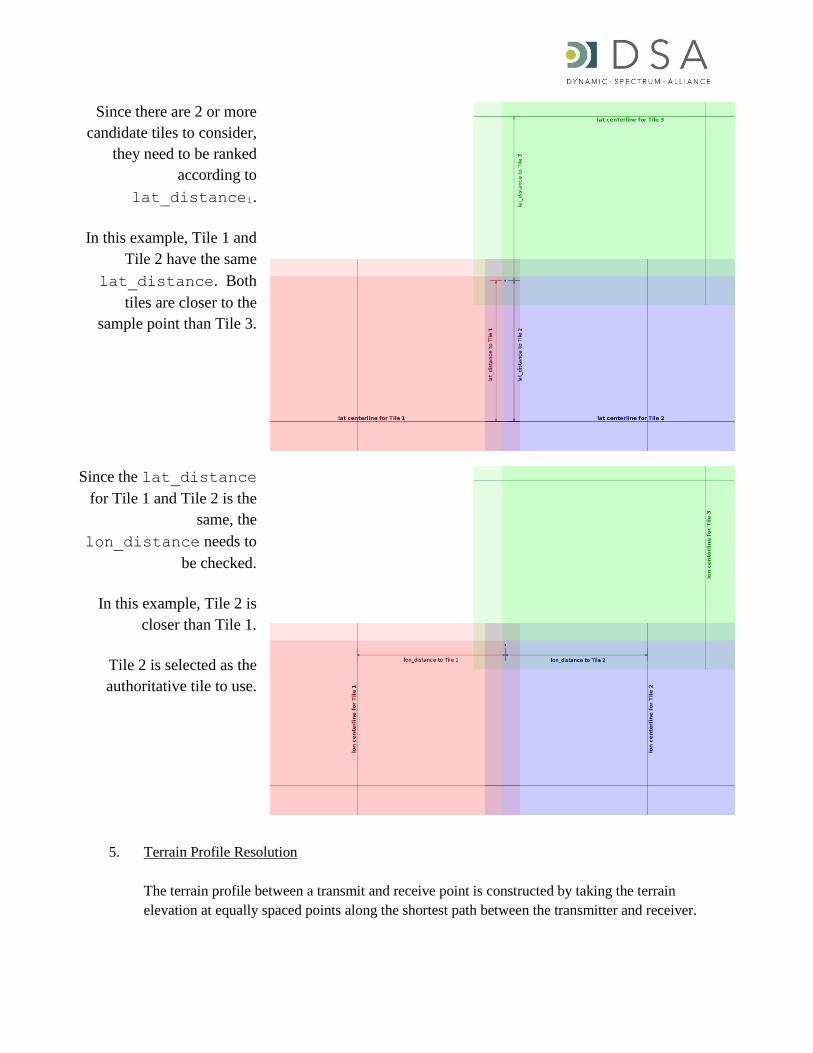
Since there are 2 or more

candidate tiles to consider,

they need to be ranked

according to

lat_distancei.

In this example, Tile 1 and

Tile 2 have the same

lat_distance. Both

tiles are closer to the

sample point than Tile 3.

Since the lat_distance

for Tile 1 and Tile 2 is the

same, the

lon_distance needs to

be checked.

In this example, Tile 2 is

closer than Tile 1.

Tile 2 is selected as the

authoritative tile to use.

5. Terrain Profile Resolution

The terrain profile between a transmit and receive point is constructed by taking the terrain

elevation at equally spaced points along the shortest path between the transmitter and receiver.

The shortest path is computed using the Vincenty algorithm10. The nominal spacing of the bins in

the terrain profile is 50 meters. Note that the terrain profile spacing is independent of the

underlying terrain grid size. Bilinear interpolation is used to fill points in the terrain profile as

described in section 4 above.

III. Calculations

White space spectrum availability calculations are location-specific. For the purpose of

discussion in this section, the WSD is assumed to be at a point W0, which has a latitude of W0,lat,

a longitude of W0,lon, and a height of W0,h (optional).

1. Compute frequencies that are “in use” by protected services

1.1. Identify all of the protected entities that are within 300 km of point W0.

1.2. If the height of W0 is not available, then assume that W0,h = 10 meters above

ground.

1.3. For each protected entity, apply the point-to-point propagation model prescribed

in Annexes A and B to predict the residual power level of each entity at point W0.

Example

1.3.1. For a TV transmitter Ti, compute the effective radiated power (Pi,radiated) of Ti in

the direction of W0, including any antenna pattern adjustments.

1.3.2. Use propagation modeling to compute the path loss (LTi) between Ti and W0.

1.3.3. Compute the effective ambient signal power at point W0 as

Pi,eff = Pi,radiated - LTi

1.3.4. If Pi,eff is greater than the SNR limit plus link margin for TV transmitters, then this

channel is considered to be “in use” by Ti, otherwise the signal is too weak and this

channel is considered to be “not in use” by Ti.

2. For each “in use” protected service, use the adjacent channel rejection ratios relative to Pi,eff

to compute the power constraints that should be applied to White Space Devices.

10 The Vincenty inverse algorithm (http://www.ngs.noaa.gov/PUBS_LIB/inverse.pdf) computes

the shortest ellipsoidal path between two points on an oblate spheroid (like the WGS84 reference

model of the Earth).

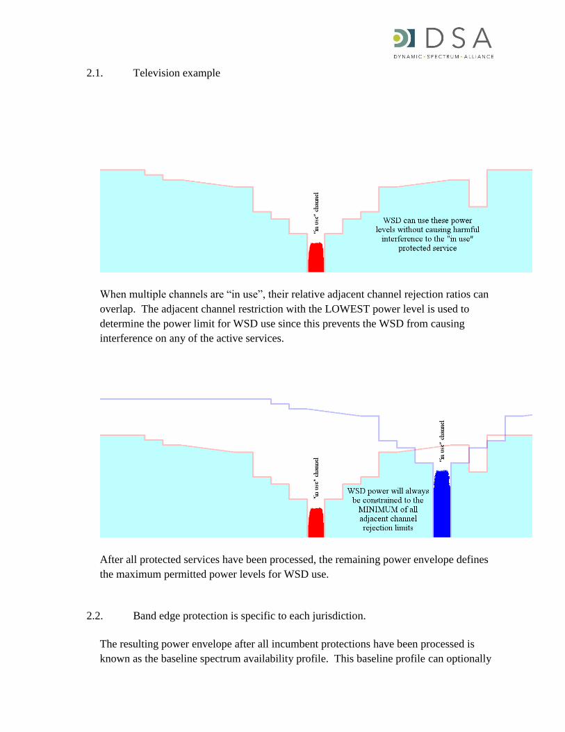
2.1. Television example

When multiple channels are “in use”, their relative adjacent channel rejection ratios can

overlap. The adjacent channel restriction with the LOWEST power level is used to

determine the power limit for WSD use since this prevents the WSD from causing

interference on any of the active services.

After all protected services have been processed, the remaining power envelope defines

the maximum permitted power levels for WSD use.

2.2. Band edge protection is specific to each jurisdiction.

The resulting power envelope after all incumbent protections have been processed is

known as the baseline spectrum availability profile. This baseline profile can optionally

be processed further to compensate for the WSD emission masks as described in section

3.1.

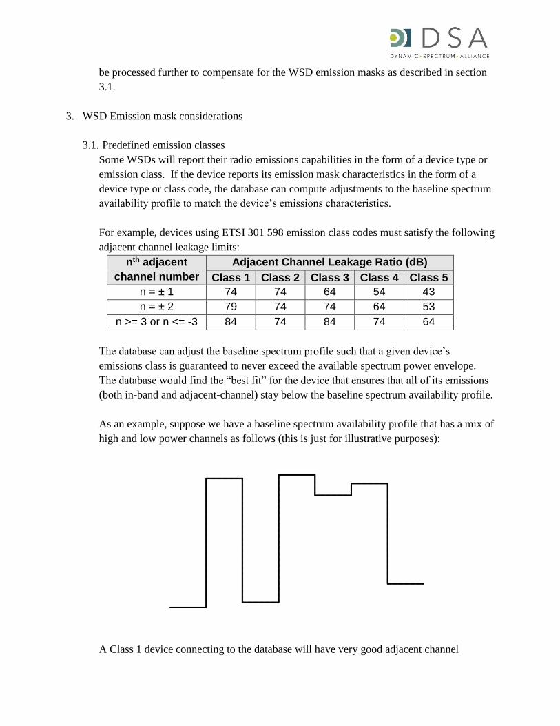
3. WSD Emission mask considerations

3.1. Predefined emission classes

Some WSDs will report their radio emissions capabilities in the form of a device type or

emission class. If the device reports its emission mask characteristics in the form of a

device type or class code, the database can compute adjustments to the baseline spectrum

availability profile to match the device’s emissions characteristics.

For example, devices using ETSI 301 598 emission class codes must satisfy the following

adjacent channel leakage limits:

nth adjacent

channel number

Adjacent Channel Leakage Ratio (dB)

Class 1 Class 2 Class 3 Class 4 Class 5

n = ± 1 74 74 64 54 43

n = ± 2 79 74 74 64 53

n >= 3 or n <= -3 84 74 84 74 64

The database can adjust the baseline spectrum profile such that a given device’s

emissions class is guaranteed to never exceed the available spectrum power envelope.

The database would find the “best fit” for the device that ensures that all of its emissions

(both in-band and adjacent-channel) stay below the baseline spectrum availability profile.

As an example, suppose we have a baseline spectrum availability profile that has a mix of

high and low power channels as follows (this is just for illustrative purposes):

A Class 1 device connecting to the database will have very good adjacent channel

leakage performance, so it will be able to emit relatively high power levels and still stay

beneath the permitted power envelope.

A Class 5 device will have a worse adjacent channel leakage performance, so it will need

to have it’s power levels reduced in order to stay within the bounds of the permitted

power envelope.

Class 1 emission class Class 5 emission class

The database adjusts the spectrum response according to the class of device making the

query, and ensures that the devices can never exceed the baseline spectrum profile.

In this example, a Class 1 device will receive a response from the database that is very

close to the baseline spectrum profile because it has a very good emission mask that

guarantees that it will not exceed the baseline power limits.

For the Class 5 device, the database has to reduce the power on some channels to make

sure the device’s adjacent channel leakage stays below the baseline power limits. Each

device class will receive an answer from the database tailored to its particular emission

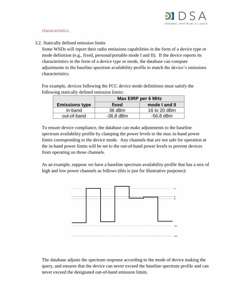
characteristics.

3.2. Statically defined emission limits

Some WSDs will report their radio emissions capabilities in the form of a device type or

mode definition (e.g., fixed, personal/portable mode I and II). If the device reports its

characteristics in the form of a device type or mode, the database can compute

adjustments to the baseline spectrum availability profile to match the device’s emissions

characteristics.

For example, devices following the FCC device mode definitions must satisfy the

following statically defined emission limits:

Emissions type

Max EIRP per 6 MHz

fixed mode I and II

in-band 36 dBm 16 to 20 dBm

out-of-band -36.8 dBm -56.8 dBm

To ensure device compliance, the database can make adjustments to the baseline

spectrum availability profile by clamping the power levels to the max in-band power

limits corresponding to the device mode. Any channels that are not safe for operation at

the in-band power limits will be set to the out-of-band power levels to prevent devices

from operating on those channels.

As an example, suppose we have a baseline spectrum availability profile that has a mix of

high and low power channels as follows (this is just for illustrative purposes):

The database adjusts the spectrum response according to the mode of device making the

query, and ensures that the device can never exceed the baseline spectrum profile and can

never exceed the designated out-of-band emission limits.

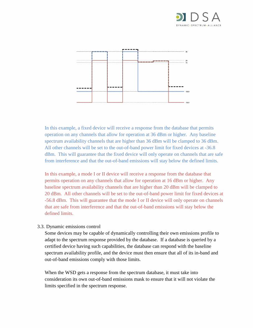
In this example, a fixed device will receive a response from the database that permits

operation on any channels that allow for operation at 36 dBm or higher. Any baseline

spectrum availability channels that are higher than 36 dBm will be clamped to 36 dBm.

All other channels will be set to the out-of-band power limit for fixed devices at -36.8

dBm. This will guarantee that the fixed device will only operate on channels that are safe

from interference and that the out-of-band emissions will stay below the defined limits.

In this example, a mode I or II device will receive a response from the database that

permits operation on any channels that allow for operation at 16 dBm or higher. Any

baseline spectrum availability channels that are higher than 20 dBm will be clamped to

20 dBm. All other channels will be set to the out-of-band power limit for fixed devices at

-56.8 dBm. This will guarantee that the mode I or II device will only operate on channels

that are safe from interference and that the out-of-band emissions will stay below the

defined limits.

3.3. Dynamic emissions control

Some devices may be capable of dynamically controlling their own emissions profile to

adapt to the spectrum response provided by the database. If a database is queried by a

certified device having such capabilities, the database can respond with the baseline

spectrum availability profile, and the device must then ensure that all of its in-band and

out-of-band emissions comply with those limits.

When the WSD gets a response from the spectrum database, it must take into

consideration its own out-of-band emissions mask to ensure that it will not violate the

limits specified in the spectrum response.

A device might have different out-of-band emission characteristics depending on its

quality of design (e.g., high-end vs. low-end components), or it may use a technology that

supports multiple modulation types (e.g., Wi-Fi supports up to 76 different modulation

coding schemes), or there might be other factors that cause the emissions profile to

change depending on current operating conditions. In each of these situations, it is up to

the WSD to ensure that its emissions profile is compliant with the database’s spectrum

response under all modes of operation.

Figure 3: Example of WSD emissions profile being considered in conjunction with the

power envelope provided by the spectrum database.

The WSD could employ any number of techniques to ensure compliance with the

database’s spectrum response, including, but not limited to, reducing output power,

changing modulation types, switching filters, shrinking occupied bandwidth, etc.

Annex D: Information Regarding ITU-R. P-1812

I. Introduction

The Suggested Technical Rules and Regulations for the Use of Television White Spaces

contemplate that available frequencies and maximum transmit power for a white space

device at a given location may be determined based on a geolocation and database

method. In particular, database(s) designated by the regulator will provide this

information based on the positional information from a master white space device, the

height of the transmitting antenna (for fixed master devices), and use by licensed

incumbents in or near the geographic area of operation of the white space device. The

rules suggest that a database will supply a list of available frequencies and associated

permitted transmit powers to white space devices pursuant to the algorithm in Annexes A

and B or pursuant to the algorithm set forth in this Annex. Annex C can be used with

either Annexes A and B or this Annex.

Annexes A and B are based on the Longley-Rice propagation model. However,

other point-to-point, terrain-based propagation models may also serve as the basis for

spectrum availability calculations. One such model is the International

Telecommunication Union’s Radiocommunication Sector Recommendation P-1812

(ITU-R. P-1812). Like Longley-Rice, ITU-R. P-1812 is a path-specific propagation

prediction method for point-to-area terrestrial services in the VHF and UHF bands.

Further detail regarding ITU-R. P-1812, including the model itself and an explanation of

its implementation is available for download on the ITU’s website at

https://www.itu.int/rec/R-REC-P.1812-3-201309-I/en.