sunk costs hysteresis in spanish manufacturing exports
TRANSCRIPT

Sunk costs hysteresis in Spanish manufacturing exports
Juan A. Máñez Castillejo
María E. Rochina Barrachina
Juan A. Sanchis Llopis
Universidad de Valencia and LINEEX
April-2005
Corresponding author: Juan A. Máñez-Castillejo Universidad de Valencia Facultad de Economía Departamento de Economía Aplicada II Avda. de los Naranjos s/n 46022 Valencia (Spain) Phone: 0034 963828356 Fax: 0034 963828354 E-mail: [email protected]
Acknowledgements: Financial support from the Instituto Valenciano de Investigaciones Económicas and the Ministerio de Ciencia y Tecnología (SEC2002-03812) is gratefully acknowledged. We would also like to thank Fundación SEPI for providing the data.
1
Sunk costs hysteresis in Spanish manufacturing exports
Abstract
This paper tests the sunk costs explanation for hysteresis in exports using a
sample of Spanish manufacturing firms for the period 1990-2000, allowing for
sunk costs to be different for small and large firms. The data are drawn from the
Spanish Encuesta sobre Estrategias Empresariales. To obtain consistent
estimates for sunk costs, we control for all other sources of persistence and use a
dynamic random effects multivariate probit model that is estimated through
pseudo simulated maximum-likelihood techniques. Our results support the sunk
costs explanation for hysteresis for both size groups and indicate that sunk costs
are smaller for large firms. Furthermore, some firm characteristics such as size,
productivity or vertical and horizontal product differentiation are found to have a
significant influence on the probability of exporting.
Key words: hysteresis in trade, sunk costs, firm size, dynamic discrete choice
models
JEL classification: F12, L1, C23, C25

2
1. Introduction.
In the analysis of the decision to export it seems sensible to think that firms face
costs associated with entering foreign markets that may be sunk in nature. For
instance, non-exporting firms have to research foreign demand and competition,
establish marketing and distribution channels, adjust their product
characteristics and packaging to meet foreign tastes and/or fulfil quality and
security legislation of other countries.
Acknowledging the existence of sunk costs implies that current exports
depend on past export trajectories and, more interestingly, that transitory
changes in trade policy or conditions may lead to permanent changes in market
structure, that is, sunk entry or exit costs produce hysteresis in export flows.1
Furthermore, when there is uncertainty about market conditions, the existence of
sunk costs affects the entry and exit patterns as trade flows are less responsive to
changes in market conditions, such as exchange rates or incentives (subsidies)
for exports.
It is important to note that although persistence in exporting status might
be caused by sunk costs, it might also be due to either underlying (observed and
unobserved) firm heterogeneity or serial correlation in transitory shocks to
exporting profits. Therefore, in order to identify the role of sunk costs one would
need an econometric framework that allows controlling for all competing sources
of persistence in export behaviour.
The first attempt to tackle the sunk-cost hysteresis hypothesis in the
empirical literature on exporting is Roberts and Tybout (1997), who directly
analyse entry and exit patterns using plant-level panel data for Colombian
manufacturing. More recent empirical evidence on sunk costs hysteresis are
Bernard and Wagner (1998), Bernard and Jensen (2004) and Campa (2004), for
German plants, U.S. plants and Spanish firms, respectively.
The objective of this paper is to assess the importance of sunk costs
hysteresis examining the decision of firm export participation and to test whether
1 The theoretical literature on sunk costs and exporting was developed by Dixit (1989a,b), Baldwin
(1988), Baldwin (1989), Baldwin and Krugman (1989) and Krugman (1989).

3
sunk costs differ between large and small firms, using panel data for Spanish
manufacturing firms, drawn from the Encuesta sobre Estrategias Empresariales
(hereafter, ESEE), for the 1990s. To account for different causes of persistence we
implement a dynamic random effects multivariate probit model, which is
estimated by simulated maximum likelihood techniques.
The main contributions of our work to the existing literature are the
following. First, we use an extensive set of firm specific and market
characteristics to account for observed firm/market heterogeneity, paying special
attention to vertical and horizontal product differentiation, and spillovers.
Secondly, whereas previous works impose a structure on the serial correlation of
transitory shocks (Roberts and Tybout, 1997, Bernard and Wagner, 1998, and
Bernard and Jensen, 2004), we allow for a free serial correlation. Misspecification
problems may arise from a given structure and may lead to inconsistent
estimates for sunk costs. Thirdly, different to other empirical studies using plant
data (Roberts and Tybout, 1997, Bernard and Wagner, 1998, and Bernard and
Jensen, 2004), we have firm data, which are the observation units appropriate for
modelling the export decision. Finally, a novelty in the existing literature is that
we allow the coefficients controlling for sunk costs to differ between small and
large firms. If some unobserved characteristics determining sunk costs of
entering export markets are linked to the size group to which the firm belongs, we
expect sunk costs to vary between size groups. For example, other things being
equal, if large firms have advantages in establishing international networks,
acquiring information, they benefit from organizational advantages, or they enjoy
economies of scope in exports they should face smaller sunk costs.
As in Campa (2004) we also analyse the decision to export by Spanish
firms. However, our work differs from Campa´s (2004) in the following respects.
First, when modelling the export decision Campa (2004) considers a limited set of
firm and market characteristics. By widening this set, identification of sunk costs
is improved.2 Secondly, Campa´s (2004) estimation method does not allow for
serial correlation in transitory shocks. As such, this unmodeled persistence in the
2 As specifically stated by Campa (2004), his paper does not focus on the characteristics of the firms
that enter or exit the export market. His main focus is the responsiveness of Spanish export supply
to changes in the exchange rate.

4
error structure may have been picked up by the variables capturing past
exporting trajectories and thus incorrectly interpreted as sunk costs. However,
our estimation method allows for this serial correlation. Thirdly, whereas our
work considers data from 1990 to 2000, the sample period in Campa (2004) only
covers until 1997. Finally, Campa´s (2004) restriction about sunk costs being
independent of the firm´s history prior to the previous year prevents him from
examining the speed of depreciation of the exporting experience. Our analysis, by
allowing sunk costs to be a function of a longer exporting history and to differ
between size groups, improves the understanding of the dynamics of participation
in foreign markets.
Our results suggest that, even after controlling for unobserved firm
heterogeneity and serial correlation in transitory shocks, sunk costs and observed
firm heterogeneity are important determinants of the export decision. Hence, we
find evidence to support the sunk costs explanation of the hysteresis hypothesis.
Our results also indicate that large firms have smaller sunk costs than small
firms, but both size groups share a rapid depreciation of their exporting
experience if they leave the export market. Furthermore, we find that firms which
are larger, more productive and have higher R&D and advertising intensities
enjoy a higher probability of exporting.
These findings contribute to better understand the determinants of the
firm’s decision to export and suggest possible export promotion policies. On the
one hand, policies oriented to improve information and access to foreign markets
by providing exporting infrastructures could reduce the sunk costs of entry,
which are especially relevant for small firms. On the other hand, policies directed
at increasing productivity or stimulating product differentiation behaviours would
have a positive impact on exporting.
The rest of the paper is organised as follows. In section 2 we present the
data and analyse export patterns for Spanish manufacturing. Section 3 is devoted
to modelling, estimation issues and variables. The estimation results are
summarised in section 4. Finally, section 5 concludes.

5
2. Data and export patterns.
2.1. The data.
We use data drawn from the ESEE, a representative annual survey of Spanish
manufacturing firms carried out since 1990, which includes exhaustive
information at the firm level.
The sampling procedure of the ESEE is the following. In the base year,
1990, firms were chosen using a selective sampling scheme with different
participation rates depending on firm size. All firms with more than 200
employees (large firms) were requested to participate and the participation rate
reached approximately 70% of the number of firms in the population. Firms that
employed between 10 to 200 (small firms) were randomly sampled by industry
and size strata, holding around 5% of the population.3 Hence, the coverage of the
dataset is different depending on the size group of firms. The different sampling
properties of these two size groups as well as the possible relationship between
size and the export decision advice to carry out a separate analysis of the
representativeness of the sample and export patterns by size group.
We select a panel of continuously operating firms over the period 1990-
2000. The choice of a continuous panel is motivated by two reasons. First, to
analyse firm´s export trajectories for the maximum length of time, we sample out
those firms that fail to supply export information in any year. Second, to estimate
a dynamic specification with lagged endogenous variables, we need to build up a
panel as long as possible. Furthermore, we drop any firm that failed during the
sampling period.4 After applying these criteria, we end up with a balanced panel
of 755 firms.
3 Firms with less than 10 employees in 1990 were not included in the survey. 4 Including these firms would involve to model the probability of failing and would substantially
complicate the analysis. However, this assumption is not innocuous, as shown in Esteve, Sanchis
and Sanchis (2004), where using a sample drawn from the ESEE, they find that exporting firms are
less likely to fail.

6
Table 1 shows that, in our sample, small firms are slightly over-
represented when compared to the complete sample: in 1990, their proportion in
total firms and their shares in total employment, sales and exports are larger.
[Insert Table 1 about here]
Table 2 shows that, regardless of size group, firms in our sample are
smaller (as measured by the number of employees) and export a higher
proportion of their sales than firms in the complete sample. However, other
relevant characteristics such as the sample probability of being an exporter/non-
exporter or the share of exporting firms on total sales and employment are similar
in both samples. We therefore consider that our sample is suitable to estimate the
probability of exporting.
[Insert Table 2 about here]
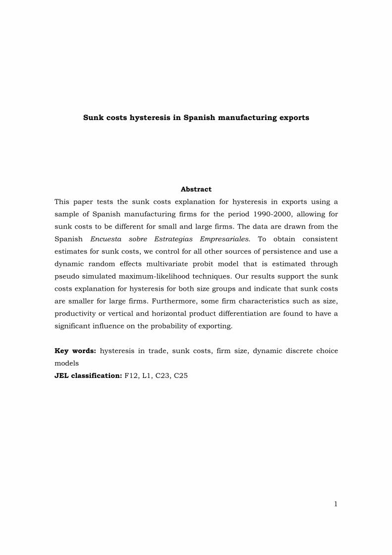
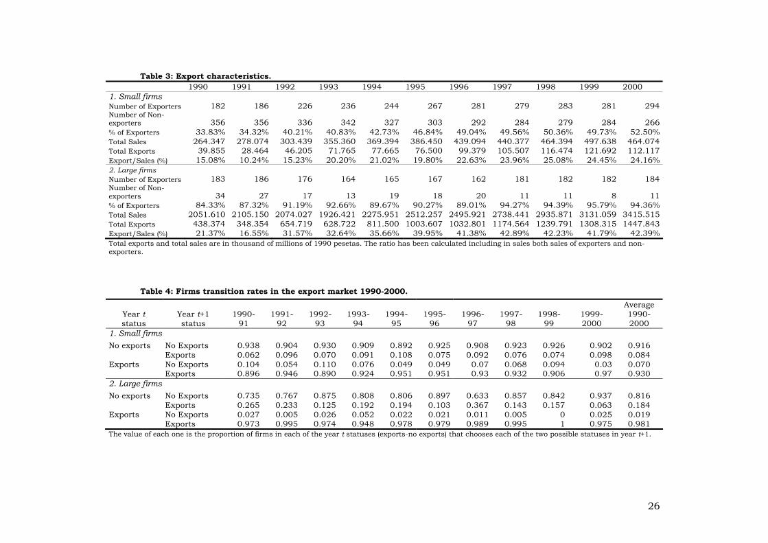
Table 3 reports characteristics of our sample on export activity, by size
group, for the period 1990-2000. The proportion of exporting firms steadily
increased for both groups along the period (for small firms it rose from 33.83% to
52.50% and for large firms from 84.33% to 94.36%), although such proportion
always remained higher for large firms. This could be suggesting that sunk costs
of entering the export markets are smaller for large firms.
At the same time, the participation of exports on sales grew much faster for
large firms than for small ones. This is explained by two factors: first, the annual
growth rate of exports is larger for large firms than for small ones (11.95% and
10.34%, respectively) and secondly, the annual growth rate of sales is larger for
small firms than for large ones (5.63% and 5.10%, respectively). Hence, whilst the
fraction of exports on sales for large firms is under 1.5 times that for small firms
(21.37% and 15.08%, respectively) in 1990, it is almost double (42.39% and
24.16%, respectively) by 2000.
[Insert Table 3 about here]

7
2.2. Entry and exit patterns in the export market.
To evaluate the importance of the flows in and out of the export market, we
analyze sample transition rates (Table 4).5 Each one of the entries in this table
gives the proportion of firms in each of the year-t statuses (export versus non
export) that choose each of the two possible statuses in year t + 1.
The second and third rows of each panel of Table 4, which report the entry
and exit rates in/from the export market (i.e., transitions from no exports to
exports and from exports to no exports), show that exporting one year does not
necessarily mean permanence in this activity. For the group of small firms, the
average entry and exit rates are quite similar (8.4% and 7%, respectively) and
some years the exit rate exceeds the entry rate, suggesting a high rate of
turnover. For large firms, the average entry rate is above 18% and the exit rate
under 2%, pointing out a clear trend of incorporation to the export market and of
persistence in that status. Hence, it is very likely that once a large firm starts
exporting remains doing so. As a result of these entry and exit rates, there is a
net gain of 113 exporters (99 out of the 356 non-exporters classified as small in
1990 and 14 out of the 34 non-exporters classified as large, see Table 3). In
population terms, this means a net gain of 2000 firms (1980 small and 20 large),
suggesting that export became a general activity during the analyzed period.6
[Insert Table 4 about here]
Together with the substantial entry and exit, there is an important degree
of persistence in the exporting status: 63.01% of small firms and 77.41% of large
firms never change their exporting status.7 Columns 1 and 2 of Table 5 present
the proportion of exporters and non-exporters in 1990 that had the same status
in one of the subsequent 10 years.8 The percentage of small firms that exported in
5 For the purpose of calculating transition rates, firms have been split into size groups according to
their employment in 1990. The alternative of using current employment could lead to transition
rates higher than 100%, since a number of firms move from the small to the large group and
viceversa over time. 6 These figures have been calculated taking into account the sampling scheme of the ESEE. 7 These figures have been calculated accounting for the firms that always or never export. 8 We follow Bernard and Jensen (2004) to build up this table. In these columns we do not
distinguish between firms that export (not export) continuously and firms that change status. For

8
1990 and were also exporting in 1995 is slightly above 90% (five years later this
percentage is exactly the same). For large firms persistence is even more intense
as 94% of the firms exporting in 1990 also exported in 1995 and five years later
this percentage is even larger, 95.6%. Persistence in the non-exporting status,
though important, is not as intense as in the exporting status. Almost 77% of
small firms that did not export in 1990 did not export five years later, and 67.1%
did not export in 2000. Among large firms, persistence in the non-exporting
status is even lower as the aforementioned percentages get reduced to almost
53% and 35.3%, respectively. This lower rate of persistence for large firms in the
non-exporting status confirms the trend of incorporation to the export market
detected above.
[Insert Table 5 about here]
Columns 3 and 4 of Table 5 report the predicted rates of persistence in
each of the two statuses. These are calculated using the annual transition rates
given by the data and presented in Table 4. Regardless of size group, and over the
whole sampling period, predicted persistence is lower than (sample) actual
persistence. Hence, we can extract two conclusions: first, the probability of
exporting is higher for firms that have exported before, i.e. there is a high rate of
re-entry by former exporters; secondly, firms in the export market with a non-
exporting past have a higher probability of leaving the export market. We observe
higher (lower) persistence rates in exporting (non-exporting) status for large firms
than for small firms.
So far we have detected that export participation shows a high level of
persistence across firms in the sample by size group. Now, we analyze if there
exists heterogeneity of entry and exit rates across industries. Figure 1 shows
average annual firm entry and exit rates for the 20 manufacturing sectors of the
NACE-93 classification and the overall sample of firms.9 While some industries
exhibit turnover patterns that are similar to the overall sample, other industries
(such as leather and shoes, printing and printing stuff, rubber and plastic
products, metallurgy, office machines, motors and cars, other transport
example, in the percentage of 1996 we include both firms that exported every year from 1990 to
1996 and firms that exported in 1990 and 1996, but not in one or more of the years in between. 9 The industry classification can be found in at the bottom of Table 6.

9
materials, furniture or other manufacturing goods) show entry or exit rates that
substantially differ from those of the overall sample.10 This suggests that
firm/market characteristics are likely to be important determinants of the export
decision.
[Insert Figure 1 about here]
The aim of next section is to present an econometric model to investigate
the role of sunk costs and firm and industry characteristics in explaining
observed exporting status persistence. Furthermore, the observed differences
between the patterns of persistence for large and small firms suggest to check
whether sunk costs differ between the two size groups.
3. Modelling and estimation.
3.1. Modelling the export decision.
We follow Roberts and Tybout (1997) in modelling the decision to export by a
rational, profit-maximizing firm. The firm considers expected profits (net of entry
and exit sunk costs) derived from that decision. In each period t the variation in
gross profits adjusted for sunk costs is given by
( ) ( )π π − − −=
= − − − − − − ∑ %0 0, 1 , , 1
2
ˆ , (1 ) (1 )iJ
jit it it t it it i t it it i t j it i t it
jy p s F y F F y G y y (1)
where yit takes the value of 1 if the firm exports in period t and 0 otherwise. π it is
the current increase to gross profits associated with the decision to export; firm-
specific characteristics, market characteristics and spillovers are included in its ;
and other factors, such as aggregate exchange rate movements, trade policy
conditions, etc., are included in tp . Ji is the age of the firm and
( )( )−
− − −== −∏%
1, , ,1
1ji t j i t j i t kk
y y y summarizes the firm recent export experience and
takes the value of 1 if the last period that firm i exported was period −t j and 0
otherwise. To account for sunk costs the following assumptions are made. First, a
firm that has never exported faces an entry cost of 0itF and would earn the first
10 An extreme case is the office machines sector, with no change of exporting status over the period.

10
year exporting ( )π − 0,it it it itp s F . Second, a firm that exported in the previous year,
i.e. if yi,t-1=1, does not have to pay the entry cost in t and would earn ( )π ,it t itp s ,
but if this firm decides to exit it would incur in an exit cost represented by − itG .
Finally, firms that abandon the export activity in previous periods (t - j with ≥ 2j )
and decide to re-start exporting again are also considered. In this case, we
assume that the firm faces a re-entry cost of jitF , which would leave the firm
earnings ( )π −, jit i it itp s F . The j subscript indicates that re-entry costs depend on
the length a firm has been away from exporting. This could reflect the
depreciation of knowledge and experience accumulated during the exporting
period or the increasing cost of updating products, market channels, etc., to the
“changing” foreign markets.
We assume that in period t managers plan the firm export participation
sequence that maximises the expected current and discounted future profits net
of sunk costs.11 This maximised payoff is,
δ π∞=
∞−
=
=
∑max ˆ
is s t
s tit t is
y s tV E (2)
where Et is an expectations operator conditioned on the set of firm information at
time t and δ is a time discount rate. Firm i chooses the current yit value that
satisfies the Bellman´s equation:
π δ + − =
= + , 1 0max ˆ i
it
J
it it t i t it j jyV E V y . (3)
A firm that decides to export in t gets the expected present value of payoffs
( ) ( )π δ + − − −==
+ = − − − −∑ %0 0, 1 , 1 ,1
2
1, (1 )i
iJJ j
it t i t it it j it i t it it i t jjj
E V y y F y F F y (4)
and one that decides not to do it
( )δ + − −== −, 1 , 11
0, iJ
t i t it it j it i tjE V y y G y . (5)
The ith firm will decide to export during period t whenever (4) minus (5) is
positive, i.e.
11 We assume that the firm also chooses the profit-maximizing level of exports if it decides to export.

11
( ) ( ) ( ) ( )π δ + + − −=
+ = − = − + + − − ≥ ∑ %0 0 0, 1 , 1 , 1 ,
21 0 0.
iJj
it t i t it t i t it it it it i t it it i t jj
E V y E V y F F G y F F y
(6)
The empirical specification is derived from (6). Defining the latent variable
π *it as current gross operating profits plus the discounted expected future return
from being an exporting firm in year t,
( ) ( )π π δ + + = + = − = *
, 1 , 11 0it it t i t it t i t itE V y E V y (7)
export participation is then given by the following dynamic discrete choice
process:
( ) ( )π − −=
− + + − − ≥=
∑ %* 0 0 0, 1 ,
21 0
0 .
iJj
it it it it i t it it i t jjit
if F F G y F F yy
otherwise (8)
We approximate π −* 0it itF as a reduced-form expression on exogenous
firm/market characteristics and spillovers (Xit), macro conditions ( µt ), and noise
(ε it ).12 Therefore,
π µ β ε− = + +* 0it it t it itF X . (9)
We also consider some identifying assumptions in relation to sunk entry,
re-entry and exit costs. First, we assume that sunk costs do not vary across time.
Second, we suppose that sunk entry costs for firms which did not export for at
least J years are the same, =0 0iF F , and that all firms which did not export for j <
J years incur in the same re-entry sunk costs, =j jiF F . Finally, we consider that
all firms currently exporting have the same exit cost =iG G .
Using the above assumptions, re-defining γ− =0 j jF F for j = 2,…,J,
γ+ =0 0F G , and substituting (9) into (8), we have the estimation equation:
µ β γ γ ε− −=
+ + + + ≥=
∑ %0, 1 ,
21 0
0 otherwise.
Jj
t it i t i t j itjit
if X y yy (10)
This equation can be adjusted to make sunk costs specific to size group. To
do so we interact the lagged variables structure (that captures sunk costs) with
12 All of them, with the exception of ε it , are assumed to be observable to the firm in period t.

12
the size group the firm belongs to. Then our final estimation equation is as
follows,
µ β γ γ γ τ γ τ ε− − − − − −= =
+ + + + + + ≥=
∑ ∑% %0 0, 1 , , 1 ,
2 21 0
0 otherwise,
J Jj j
t it s i t s i t j l s i t l s i t j itj jit
if X y y y yy (11)
where τ is 1 for large firms and 0 for small ones. +0F G is γ 0s for small firms and
γ γ −+0 0s l s for large firms. Finally, −0 jF F is γ j
s for small firms and γ γ −+j js l s for large
firms.
Notice, from last expression, that the export decision in t does not depend
on the firm exporting background if sunk costs are zero. This allows checking for
the importance of sunk costs: for small firms, we have to test whether 0sγ and j
sγ
are jointly equal to zero; for large firms we check whether 0 0s l sγ γ −+ and j j
s l sγ γ −+
are jointly equal to zero (for j = 2,…, J). It is also possible to analyse the rate of
depreciation of experience and accumulated knowledge in export activities by
looking at the coefficients for large and small firms individually.
3.2. Estimation issues.
Given that we are interested in isolating the effects of sunk costs hysteresis (true
state dependence) in the exporting status, it is crucial to control for all other
sources of persistence. Most of this task is accomplished by including the vector
of observable characteristics itX in (11). However, it is highly probable that there
still remain unobserved factors causing persistence such as product attributes,
foreign contacts, managerial ability or technology. Since they are potentially
permanent, or highly serially correlated, in practice we assume that ε it in (11) has
two components, a permanent firm-specific effect ( iα ) and a transitory component
( itu ). Hence, we allow for two sources of serial correlation in itε , the first arising
from the permanent component and the second from serial correlation in
transitory shocks to exporting profits. We further assume that the
( )ε = ∀cov , 0 , it itX i t , and normalize ( )ε =1itVar .

13
It is also needed to address an “initial conditions” problem. We observe a
firm exporting status in years 1 through T, and our lag structure reaches back J
periods. Values corresponding to the first J years ( 1,...,i iJy y ) cannot be treated as
exogenous determinants of ity , when t > J, because each one depends on αi and
previous realizations of uit, both of which are correlated with ε it . Heckman (1981)
suggests dealing with this initial conditions problem by using an approximate
representation for ity when t ≤ J. Specifically, let us suppose that expected profits
in the export market during the J pre-sample years can be represented by the
equation
π λ ε− = +* 0 p pit it it itF X (12)
where pitX is a distributed lag in pre-sample realizations on exogenous
variables.13 Then, presample export-participation is described by
λ ε+ ≥=
1 if 0
0 otherwise
p pit it
itX
y (13)
instead of equation (11). We assume that ε pit has the same properties than ε it .
Furthermore, it is assumed that the joint distribution of ε ε ε ε+1 1,..., , ,...,P Pi iJ iJ iT is
multivariate standard normal, and its full correlation matrix is characterised by
( ){ }× − /2T T T free distinct (and estimable) correlations, with ones on the
diagonal and ρ ρ=ts st as off-diagonal elements.14 Roberts and Tybout (1997),
Bernard and Wagner (1998) and Bernard and Jensen (2004) impose an AR(1) on
the serial correlation of the transitory components of ε it and ε pit . Campa (2004)
does not allow for correlation of these components. Nevertheless, we leave it fully
unrestricted.
Positive (negative) signs in the set of correlation coefficients between the
disturbances of the first J periods and the disturbances in every other period,
indicate that firms that were more likely to be exporters in initial conditions years
were more (less) likely to remain exporters during sample years compared to the
13 In the empirical work all the firm characteristics ( itX ) are included as explanatory variables in
pitX . We also include two-year lagged values of the firm’s continuous variables.
14 In our empirical work J=3 and T=10.

14
non-exporters. If these correlation coefficients are jointly equal to zero, there is no
initial conditions problem and the model reduces its dimension to a T - J
multivariate probit model. And if , ts t sρ ∀ ≠ , are all jointly equal to zero, then
exporting equations may be estimated using simple univariate probit models. We
estimate the general model with free correlations and test for special cases.
Our general model is a dynamic random effects multivariate probit model
that we estimate using the mvprobit Stata program15 developed by Cappellari and
Jenkins (2003). This program uses simulated maximum likelihood techniques
(SML) to solve the computational problem of evaluating T-dimensional integrals.16
In addition, the program allows implementing a pseudo simulated maximum
likelihood estimator (PSML) that adjusts the estimates of the parameter
covariance matrix to take into account arbitrary correlations between all panel
observations of a given firm (see Huber, 1967 and White, 1982).
3.3. Explanatory variables.
To parameterize the firm’s exporting decision given by equation (11), we assume
that variation in export profitability and start-up costs (other than unobserved
components) may arise from four different sources: time-specific effects, industry
dummies, observable differences in firm/market characteristics and spillovers.
Time effects are included in order to capture macro-level changes in export
conditions that are common across firms, such as the influence of business cycle,
credit-market conditions, aggregate exchange rate movements (affecting relative
prices from exporting and domestic sales), trade-policy, overall changes in
demand for Spanish exports and other time-varying factors. Industry dummies to
control for unobservable characteristics of markets where firms compete, such as
market concentration, use of technology or firms´ specific behaviour by industry,
are also included.
15 This program can be obtained at SSC public domain software archive
(http://fmwww.bc.edu/RePEc/bocode/m) or, inside Stata, type “ssc install mvprobit”. 16 In particular, it uses the Geweke-Hajivassiliou-Keane (GHK) simulator to replace multivariate
standard normal probability distribution functions by their simulated counterparts, see
Hajivassiliou and Ruud (1994) and Gourieroux and Monfort (1996).

15
We also consider several hypotheses concerning the role of observable firm
characteristics. Perhaps the most obvious are those related to past success.
Although the usual claim is that better performing firms become exporters, a
substantial fraction of export policies assumes instead that exporters will become
good performing firms. To proxy for firm success we include age, size and
productivity. Age proxies for efficiency differences. If market forces select out
inefficient producers, older firms will tend to be more competitive in world
markets, either because of cost advantages that cannot be imitated by rivals or
because they have had time to move down along a learning curve.17 As pointed
out by Bernard and Jensen (1999), even if the annual payoffs from exporting were
the same for young and old firms, the young ones would perceive smaller returns
from entering the export market because they face a higher risk of failure. Size
may proxy for several effects: larger firms have been usually successful in the
past, but size may be associated with lower average or marginal costs, providing a
separate mechanism for size to increase the likelihood of exporting. Another link
between size and export may reflect scale economy-based exporting (Krugman,
1984). There are also reasons to expect firm productivity to increase the
likelihood of exporting. If the fixed costs of selling are higher in the export market
than in the domestic market or if output prices are lower, only firms with high
productivity will find it profitable to enter the export market. This is usually
referred to as the self-selection hypothesis in the models of industry dynamics.18
We discuss next the role of quality of the labour-force. If exported goods
have higher quality, a higher value to weight ratio, or require new product design
and other forms of technical assistance, then we would expect the quality of the
workforce to be positively related to entrance into foreign markets.
A sizable body of research has focused on the role of ownership in cross-
border trade. We control for the ownership structure of the firm (limited liability
corporation versus other, and foreign capital participation). One can think that
17 Roberts (1996) reports a decline in the probability of failure as a plant ages for Colombia and
Tybout (1996) reports a similar finding for Chile. The same pattern has been found in data from the
US (see Dunne et al., 1989 or Baily et al., 1992). 18 See for example, Ericson and Pakes (1995), Pakes and Ericson (1998) or Baldwin and
Rafiquzzaman (1995). Delgado, Fariñas and Ruano (2002) find evidence supporting the self-
selection hypothesis using data drawn from the ESEE.

16
non-domestically owned firms may enjoy better access to foreign markets due to
complementarities with other business within the same group. It has been
frequently argued that firms participated by foreign capital are, in general, more
efficient and so their presence in foreign markets should be higher. Furthermore,
when foreign direct investment is based on competitive advantages of the
destination market, it is expected a positive relation between foreign ownership
and exporting activity. In this case, the domestic market might be seen as a
productive platform.
The decision to export can also be affected by domestic demand factors
such as the evolution of domestic demand or the type of customer. If foreign
markets became a relevant alternative in periods of low domestic demand, we
would expect the probability of exporting to be higher in these periods. If a firm´s
main customer is the public sector (due to the nature of the product) whenever
this firm decides to export it will have to face the possible preference of the foreign
public sector for its own national producers. It can also happen that once
domestic producers have adapted their production to meet the requirements of
their domestic public sector, they may not be very much attracted by foreign
markets.
We also consider the effects of vertical and horizontal product
differentiation strategies. As vertical differentiation is related to product quality
differentiation, we proxy for it by using variables that measure the firm
innovation-related activities such as R&D intensity, complementary technological
activities and innovation results. We would expect that the higher the vertical
differentiation of the firm, the higher the probability of exporting. To account for
horizontal differentiation, which is more identified with different product
perceptions from the demand side, we include firm´s advertising intensity.
The literature on economic geography and trade (Krugman, 1992)
hypothesizes that activities of neighbouring firms may reduce entry costs. The
presence of other exporters may make it easier, for domestically oriented firms, to
break into foreign markets. A form of externality might arise if the presence of
other exporters lowers the cost of production, possibly by increasing the

17
availability of specialized capital and labour inputs. We consider three forms of
spillovers: region-specific, industry-specific and local to the industry and region.19
Finally, in order to assess the importance of sunk costs and whether they
differ between large and small firms, we use a lag structure for past participation
that reaches back three periods and takes into account the possibility of different
sunk costs according to size group. As noticed earlier, if sunk costs matter
current participation will depend upon the exporting history.
Table 6 provides detailed information on all the variables discussed above.
All nominal variables have been deflated using specific industry deflators
according to 20 sectors of the NACE-93 classification. Given that for some
variables the direction of causality remains uncertain, in the estimation we lag
one year firm characteristics and other exogenous variables to avoid possible
simultaneity problems. [Insert Table 6 about here]
4. Estimation results.
We treat the period 1991-1993 as the J = 3 pre-sample years controlling for the
initial conditions problem. The values of the variables in 1990 are included as
regressors for the 1991 initial condition. The observations for 1994-2000 are used
to estimate the relevant parameters in equation 11.
[Insert Table 7 about here]
In Table 7 we report the PSML estimates. A test for joint significance of all
the ρ -correlation coefficients leads to rejection of the null hypothesis that they
are jointly equal to zero.20 Hence, the proper estimation method involves
multivariate probit models. Furthermore, we also perform a test for endogeneity of
initial conditions by testing the joint significance of ρ -correlation coefficients
between initial conditions (1990 < t ≤ 1993) and sample years errors (1993 < t ≤
2000). Exogeneity of initial conditions is strongly rejected. Hence, initial
conditions should not be treated as exogenous.
19 See Bernard and Jensen (2004) and Clerides et al. (1998). 20 See the results of this test at the bottom of table 7. Table A.I in the Appendix reports the ρ -
correlation coefficients between time periods.

18
4.1. Time dummies, firm/market characteristics and spillovers.
We analyse the impact of time dummies, firm/market characteristics and
spillovers on the expected profits, net of sunk entry costs (π −* 0it F ), of a firm with
no previous experience in the export market. The 1995 and 2000 dummy
coefficients are positive and significant at 5% and 10% levels, respectively. The
estimate of the dummy for 1995 is probably capturing the peseta depreciation
that took place after the bandwidth widening of the European Rate Mechanism.
The dummy for 2000 could be reflecting the depreciation of the euro with respect
to the US dollar.21 In addition, the hypothesis that the time dummies are jointly
equal to zero cannot be rejected (the χ 26 test is 10.39 and the corresponding p-
value 0.109). This partial lack of responsiveness could suggest that the export
decision is rather insensitive to macro conditions during the sample period.
We also analyse the influence of observable firm/market characteristics.
Only two out of the three variables included to proxy for firm past success have
an impact on net export profitability: size (measured by the number of workers)
and productivity. Larger and more productive firms are more likely to become
exporters. The coefficient of age, often considered as a proxy for efficiency, is not
significant.22
The coefficient for the variable that proxies for labour force quality is not
significant. 23 However, this does not necessarily mean that a better quality of the
21 From 1st January 1999 exchange rates between the European Monetary Union national
currencies are fixed and euro-dollar exchange rates determine the exchange rates between national
currencies of the European Monetary Union and the US dollar. 22 Roberts and Tybout (1997), Bernard and Wagner (1998) and Bernard and Jensen (2004) find that
size affects positively the probability of exporting. Productivity appears not to be significant in most
of the specifications in Bernard and Jensen (2004). However, it is significant in most cases in
Bernard and Wagner (1998). As for age, Roberts and Tybout (1997) find that older plants are more
likely to export. The lack of significance of the variable age in our analysis may be due to the
inclusion of the variable productivity, which might be capturing differences in efficiency that in
Roberts and Tybout (1997) are picked up by the age variable. 23 Bernard and Wagner (1998) and Bernard and Jensen (2004) find significant and non significant
effects of this variable, respectively.

19
labour force will not help to succeed in the export market. A more qualified labour
force may contribute to vertically differentiate the firm product. However, the
extent of product differentiation is better captured by other vertical product
differentiation variables included in the analysis.
Neither corporate ownership nor foreign capital participation are significant
determinants of export participation.24 The result on the foreign capital
participation variable could be signalling that the aim of foreign investors is not
necessarily using Spain as a productive platform but supplying the domestic
market.
As regards the influence of domestic demand factors, the evolution of
domestic demand (measured by its growth rate) is not significant. However, firms
selling a relevant part of their production to the public sector show a lower
probability of exporting.
The probability of exporting increases with vertical product differentiation.
Two of the three variables introduced to account for this effect are significant: the
probability of exporting increases both with the intensity of R&D expenditure and
with the realization of R&D complementary activities such as quality controls or
product normalization. The third variable, which controls whether the firm
registers patents or process innovations, is not significant. This could be
suggesting that patenting does not ensure exporting success. Horizontal product
differentiation has also a positive impact on the probability of exporting, as it
shows a positive and significant coefficient for advertising intensity.
Finally, all measures of spillovers are non significant. Bernard and Jensen
(2004) introduce the same three measures of spillovers and these are always non-
significant or have a negative sign (contrary to expected).
4.2. Sunk costs parameters.
Wald tests for joint significance of the coefficients 0 2ˆ ˆ,s sγ γ and 3ˆsγ for small firms
and of the coefficients 0 0 2 2ˆ ˆ ˆ ˆ,s l s s l sγ γ γ γ− −+ + and 3 3ˆ ˆs l sγ γ −+ for large firms in (11) suggest
24 However, in Roberts and Tybout (1997) corporate ownership positively influences the probability
of exporting.

20
the rejection of the hypothesis that they are jointly equal to 0. For small firms, the
χ 23 statistic is 68.72 with a p-value approximately 0; for large firms, the χ 2
3
statistic is 38.51 with a p-value approximately 0. Hence, even after controlling for
a general form of serial correlation, exporting history matters.
Regarding individual coefficients, for small firms, the estimated coefficient
for yi,t-1 ( 0ˆsγ ) is large (2.032), positive and significant, revealing that exporting the
previous year has a strong positive impact on the probability of exporting this
year. Additionally, this coefficient can be considered as an estimate of the sum of
sunk entry costs for a firm that never exported and exit costs for current
exporters (“hysteresis band”, Dixit, 1989a). The coefficients of
γ γ− −% %2 3, 2 s , 3 sˆ ˆ ( ) and ( )i t i ty y measure, respectively, the reductions in the full sunk
entry costs faced by a new exporter enjoyed by firms that exported for the last
time two and three years ago. Both coefficients are non significant, indicating a
rapid depreciation of exporting experience; i.e. there is no significant difference
between the entry cost of a firm that last exported two or three years ago and a
firm that had never exported before.
For large firms, the “hysteresis band”, that is the coefficient of yi,t-1
( 0 0ˆ ˆs l sγ γ −+ ) is significantly smaller (1.791) than the one of small firms, but still
positive and very significant (with a p-value approximately 0). The coefficients of
γ γ γ γ− −% %2 2 3 3, 2 s l-s , 3 s l-sˆ ˆ ˆ ˆ ( + ) and ( + )i t i ty y are non significant,25 and they do not differ
significantly from 2ˆsγ and 3ˆsγ , respectively. This indicates that for large firms
exporting experience also depreciates quite fast. 26
Although sunk costs are higher for small firms and so the persistence
originated from sunk costs is larger for small firms than for large ones,
persistence in the exporting status is higher for large firms (as observed in section
2). Therefore, the higher persistence of large firms in the exporting status might
be due to other relevant sources of persistence such as differences in observed 25 γ γ2 2
s l-sˆ ˆ( + ) is 0.062, with a p-value 0.876, and γ γ3 3
s l-sˆ ˆ( + ) is 0.303, with a p-value 0.682.
26 Our results are similar to those in Roberts and Tybout (1997). Bernard and Wagner (1998) and
Bernard and Jensen (2004) include only two lags of export participation and both of them are found
to be significant. Nevertheless, it should be reminded that none of them considers the possibility of
sunk costs differing between size groups.

21
characteristics. Thus, the most relevant variables that affect positively and
significantly export market participation, such as productivity, R&D and
advertising intensity, complementary R&D or the number of employees (a
continuous measure of size) show higher average values for the group of large
firms than for the group of small firms (see Table 8). 27
4.3. Goodness of fit.
Following Roberts and Tybout (1997), to evaluate the goodness of fit of our model,
we compare actual and predicted patterns of export market participation. For the
seven-year period 1994-2000 there are 128 (that is, 27) possible export market
trajectories for an individual firm.28 Across the 755 firms of our sample, some of
these trajectories are either never observed or are quite unusual. Hence, to
simplify the comparison of actual and predicted trajectories, we group the 128
possible trajectories into 6 categories based on two criteria: first, the firm
exporting status in 1994; and second, whether the firm changes exporting status
once or more times between 1995 and 2000. Table 9 shows that actual and
predicted frequencies for the six categories are quite similar. Furthermore, the
results of a chi-square contingency table test, comparing actual and predicted
frequencies ( χ 2 =0.787 with a p-value of 0.978), indicate that there are not
significant differences between the two. These results suggest that our functional
form, lags and error structure are appropriate and that our model predicts
patterns of export market participation rather accurately.
[Insert Table 9 about here]
27 Tests of differences in means for these variables between size groups allow rejecting the equality
of mean values. 28 Actual and predicted frequencies for the complete 128 possible trajectories are shown in Table
A.II in the Appendix.

22
5. Concluding remarks.
In this paper, we test both for the existence of sunk costs in the export decision
by Spanish manufacturing firms and whether there are differences in sunk costs
between large and small firms. We use a dynamic random effects multivariate
probit model that allows controlling for competing sources of persistence: sunk
costs, heterogeneity and serial correlation in transitory shocks. The data used
have been drawn from the ESEE survey for the period 1990-2000. This survey is
representative of Spanish manufacturing firms. This paper differs from the
existing literature in the following respects. First, we use a richer set of firm
characteristics (including vertical and horizontal product differentiation variables)
and market characteristics (including industry, regional and local spillovers) that
allows for a better identification of sunk costs. Secondly, we do not impose any
structure on the serial correlation of transitory shocks. Misspecification problems
may arise from a given structure and may lead to inconsistent estimates for sunk
costs. Thirdly, whereas most previous studies use plant data, our observation
unit is the firm, which is the appropriate one to analyse the export decision.
Finally, we allow the sunk costs coefficients to vary across size groups to check
whether these costs are different between large and small firms.
We find evidence supporting the sunk cost explanation for hysteresis in
Spanish manufacturing exports and that large firms face significantly smaller
sunk costs in exporting than small firms. Furthermore, our estimation results
indicate that in both size groups those firms leaving the export market suffer a
rapid depreciation of their exporting experience. Re-entry costs that faces a firm
that last exported two or three years ago are not significantly different from those
faced by a new exporter. This phenomenon could be suggesting, for instance, that
obtaining information about foreign demand conditions is an important source of
sunk costs of entry and that this information rapidly depreciates once a firm
leaves the export market. Firm heterogeneity is also an important source of
persistence in the export market, as firm characteristics are relevant to explain
firms’ exporting trajectories. Firms’ past success (as measured by size and
productivity) has a positive impact on the probability to export. Product
differentiation also increases this probability. As regards vertical product

23
differentiation, the probability of exporting increases with the intensity of R&D
expenditure and with the realization of other R&D related activities such as
quality controls or product normalization. Firms that horizontally differentiate
their products by means of advertising also have a higher probability of exporting.
Our findings make a significant contribution to the understanding of the
determinants of firms’ decision to export and have important implications for
public policy. The combined relevance of sunk costs and firm characteristics in
the probability of exporting suggest possible export promotion policies. On the
one hand, policies directed at providing information and access to foreign markets
or providing exporting infrastructures could reduce the sunk costs of entry,
which is especially crucial for small firms. On the other hand, policies aimed to
help firms to increase productivity or to stimulate product differentiation
behaviours would have a positive impact on exporting.
References.
Baily, M.N., Charles, H., Campbell, D., 1992. Productivity dynamics in
manufacturing firms. Brookings Papers on Economic Activity, Microeconomics, pp. 187--249.
Baldwin, R.E., 1988. Hysteresis in import prices: the beachhead effect. American Economic Review 78, pp. 773--785.
Baldwin, R.E., 1989. Sunk costs hysteresis. National Bureau of Economic Research 2911.
Baldwin, R.E., Krugman, P.R., 1989. Persistent trade effects of large exchange rate shocks. Quarterly Journal of Economics 104(4), pp. 635--654.
Baldwin, J.R., Rafiquzzaman, M., 1995. Selection versus evolutionary adaptation: learning and post-entry performance. International Journal of Industrial Organization 13, pp. 501--522.
Bernard, A.B., Wagner, J., 1998. Export entry and exit by German firms. National Bureau of Economic Research 6538.
Bernard, A.B., Jensen, J.B., 1999. Exceptional exporter performance: Cause , effect, or both? Journal of International Economics 47, pp. 1-25.
Bernard, A.B., Jensen, J.B., 2004. Why some firms export? Review of Economics and Statistics 86 (2), pp. 561--569.

24
Campa, J.M., 2004. Exchange rates and trade: How important is hysteresis in trade? European Economic Review 48, pp. 527--548.
Cappellari, L. and S. P. Jenkins, 2003. Multivariate probit regression using simulated maximum likelihood, The Stata Journal, 3(3), pp. 278–294.
Clerides, S.K., Lach, S., Tybout, J.R., 1998. Is learning by exporting important? Micro-dynamic evidence from Colombia, Mexico, and Morocco. The Quarterly Journal of Economics, pp. 903--947.
Delgado, M. A., Fariñas, J. C., Ruano, S., 2002. Firm productivity and export markets: a non-parametric approach. Journal of International Economics 57, pp. 397--422.
Dixit, A., 1989a. Entry and exit decision under uncertainty. Journal of Political Economy 97(3), pp. 620--638.
Dixit, A., 1989b. Hysteresis import penetration exchange rate pass-through. Quarterly Journal of Economics 104, pp. 205--228.
Dunne, T., Roberts, M.J., Samuelson, L., 1989. The growth and failure of U.S. manufacturing plants. Quarterly Journal of Economics 105(4), pp. 671--698.
Ericson, R., Pakes, A., 1995. Markov-perfect industry dynamics: a framework for empirical work. Review of Economic Studies 62, pp. 53--82.
Esteve, S., Sanchis, A., Sanchis, J.A., 2004. The determinants of survival of Spanish manufacturing firms. Review of Industrial Organization 25, pp. 251--273.
Gourieroux, C., Monfort, A., 1996. Simulation-based econometric methods. University Press, Oxford.
Hajivassiliou, V., Ruud, P., 1994. Classical estimation methods for LDV models using simulation, in: Engle, R., McFadden, D. (Eds.), Handbook of Econometrics. North-Holland, Amsterdam, pp. 2383--2441.
Heckman, J.J., 1981. The incidental parameters problem and the problem of initial conditions in estimating a discrete time-discrete data stochastic process, in: Manski, C., McFadden, D. (Eds.), The structural analysis of discrete data. MIT Press, Cambridge, pp. 179--195.
Huber, P.J., 1967. The behaviour of maximum likelihood estimators under non-standard conditions, in: Proceedings of the Fifth Berkeley Symposium in Mathematical Statistics and Probability. University of California Press, Berkeley CA, pp. 221--233.
Krugman P.R., 1984. Import protection as export promotion: International competition in the presence of oligopoly and economies of scale, in: Kierzkowski, H. (Ed.), Monopolistic competition and international trade. University Press, Oxford, pp. 180--193.
Krugman P.R., 1989. Exchange-rate instability. MIT Press, Cambridge.

25
Krugman P.R., 1992. Geography and trade. MIT Press, Cambridge.
Pakes A., Ericson, R., 1998. Empirical implications of alternative models of firm dynamics. Journal of Economic Theory 79, pp. 1--45.
Roberts, M.J., 1996. Colombia 1977-1985: Producer, turnover, margins and trade exposure, in: Roberts, M.J., Tybout, J.R. (Eds.), Industrial evolution in developing countries: Micro patterns of turnover, productivity and market structure. University Press, Oxford, pp. 227--259.
Roberts M.J., Tybout, J.R., 1997. The Decision to Export in Colombia: An Empirical Model of Entry with Sunk Costs. American Economic Review 87, pp. 545--564.
Tybout, J.R., 1996. Chile, 1979-1986: Trade liberalization and its aftermath, in: Roberts, M.J., Tybout, J.R. (Eds.), Industrial evolution in developing countries: Micro patterns of turnover, productivity and market structure. University Press, Oxford, pp. 200--226.
White, H., 1982. Maximum likelihood estimation of misspecified models. Econometrica 50, pp. 1-25.
Tables and figures.
Table 1: Sample representativeness: large versus small firms, 1990. 1990 complete sample Continuing Sample 1990 Small firms Large firms Small firms Large firms
Number of firms 1475 709 538 217 % of total sample 67.54% 32.46% 71.26% 28.74% % of total employment 9.30% 90.70% 13.26% 86.74% % of total sales 6.71% 93.29% 11.41% 88.59% % of total exports 4.83% 95.18% 8.32% 91.68%
Table 2: Sample representativeness: exporters versus non-exporters, 1990. 1990 complete sample Continuing Sample 1990 Non-Exporters Exporters Non-exporters Exporters 1. Small firms Number of firms 1017 458 356 182 % of total sample 68.95% 31.05% 66.17% 33.83% Average size (employees) 30 58 28 56 Exports/Sales (average) - 22.70% - 22.95% % of total employment 53.15% 46.85% 49.49% 50.51% % of total sales 47.25% 52.75% 43.82% 56.17% 2. Large firms Number of firms 119 590 34 183 % of total sample 16.78% 83.22% 15.67% 84.33% Average size (employees) 452 841 349 658 Exports/Sales (average) - 21.20% - 27.23% % of total employment 9.78% 90.22% 8.98% 91.02% % of total sales 8.49% 91.51% 7.17% 92.83%
26
Table 3: Export characteristics. 1990 1991 1992 1993 1994 1995 1996 1997 1998 1999 2000 1. Small firms Number of Exporters 182 186 226 236 244 267 281 279 283 281 294 Number of Non-exporters 356 356 336 342 327 303 292 284 279 284 266 % of Exporters 33.83% 34.32% 40.21% 40.83% 42.73% 46.84% 49.04% 49.56% 50.36% 49.73% 52.50% Total Sales 264.347 278.074 303.439 355.360 369.394 386.450 439.094 440.377 464.394 497.638 464.074 Total Exports 39.855 28.464 46.205 71.765 77.665 76.500 99.379 105.507 116.474 121.692 112.117 Export/Sales (%) 15.08% 10.24% 15.23% 20.20% 21.02% 19.80% 22.63% 23.96% 25.08% 24.45% 24.16% 2. Large firms Number of Exporters 183 186 176 164 165 167 162 181 182 182 184 Number of Non-exporters 34 27 17 13 19 18 20 11 11 8 11 % of Exporters 84.33% 87.32% 91.19% 92.66% 89.67% 90.27% 89.01% 94.27% 94.39% 95.79% 94.36% Total Sales 2051.610 2105.150 2074.027 1926.421 2275.951 2512.257 2495.921 2738.441 2935.871 3131.059 3415.515 Total Exports 438.374 348.354 654.719 628.722 811.500 1003.607 1032.801 1174.564 1239.791 1308.315 1447.843 Export/Sales (%) 21.37% 16.55% 31.57% 32.64% 35.66% 39.95% 41.38% 42.89% 42.23% 41.79% 42.39% Total exports and total sales are in thousand of millions of 1990 pesetas. The ratio has been calculated including in sales both sales of exporters and non-exporters.
Table 4: Firms transition rates in the export market 1990-2000.
Year t status
Year t+1 status
1990-
91
1991-
92
1992-
93
1993-
94
1994-
95
1995-
96
1996-
97
1997-
98
1998-
99
1999-2000
Average 1990-2000
1. Small firms No exports No Exports 0.938 0.904 0.930 0.909 0.892 0.925 0.908 0.923 0.926 0.902 0.916 Exports 0.062 0.096 0.070 0.091 0.108 0.075 0.092 0.076 0.074 0.098 0.084 Exports No Exports 0.104 0.054 0.110 0.076 0.049 0.049 0.07 0.068 0.094 0.03 0.070 Exports 0.896 0.946 0.890 0.924 0.951 0.951 0.93 0.932 0.906 0.97 0.930 2. Large firms No exports No Exports 0.735 0.767 0.875 0.808 0.806 0.897 0.633 0.857 0.842 0.937 0.816 Exports 0.265 0.233 0.125 0.192 0.194 0.103 0.367 0.143 0.157 0.063 0.184 Exports No Exports 0.027 0.005 0.026 0.052 0.022 0.021 0.011 0.005 0 0.025 0.019 Exports 0.973 0.995 0.974 0.948 0.978 0.979 0.989 0.995 1 0.975 0.981 The value of each one is the proportion of firms in each of the year t statuses (exports-no exports) that chooses each of the two possible statuses in year t+1.

27
Table 5: Persistence of exporting (and Non-Exporting). Proportion of 1990 firms with the same export status.
(1) Exporters
Actual
(2) Non-exporters
Actual
(3) Exporters Expected
(4) Non-exporters
Expected 1. Small firms
1991 89.56% 93.82% 89.56% 93.82% 1992 91.75% 88.20% 84.72% 84.78% 1993 89.01% 86.80% 75.40% 78.86% 1994 87.91% 82.30% 69.62% 71.66% 1995 90.11% 76.96% 66.19% 63.93% 1996 89.56% 73.87% 62.96% 59.11% 1997 90.66% 72.19% 58.53% 53.66% 1998 91.21% 71.63% 54.54% 49.55% 1999 87.91% 71.34% 49.44% 45.89% 2000 90.11% 67.13% 47.93% 41.40%
2. Large firms 1991 97.26% 73.52% 97.27% 73.53% 1992 97.81% 58.82% 96.75% 56.37% 1993 95.62% 52.94% 94.24% 49.33% 1994 94.53% 61.76% 89.31% 39.84% 1995 93.99% 52.94% 87.39% 32.13% 1996 93.44% 52.94% 85.53% 28.81% 1997 96.17% 41.17% 84.61% 18.25% 1998 96.72% 38.23% 84.18% 15.64% 1999 96.72% 29.41% 84.18% 13.17% 2000 95.62% 35.29% 82.09% 12.35%
Note: Figures in columns (1) and (2) represent the percentage of exporting (non-exporting) firms in 1990 that were also exporting (non-exporting) in the listed year. Figures in columns (3) and (4) show the expected percentages if entering and exiting firms were chosen randomly with annual transition rates given by the data. For instance, in 1990, the number of exporters in the small firms group was 182 (see Table 3) and from Table 4 we know that the exit rate for the small firms group for the period 1990-1991 is 10.44%. Therefore, the expected number of exporters in 1991 is obtained as 182*(1-0.1044)=163, and 163 is approximately 89.56% of 182.
Figure 1: Industry average rates of entry and exit in the export market.*
02468
10121416182022
Secto
r 1
Secto
r 2
Secto
r 3
Secto
r 4
Secto
r 5
Secto
r 6
Secto
r 7
Secto
r 8
Secto
r 9
Secto
r 10
Secto
r 11
Secto
r 12
Secto
r 13
Secto
r 14
Secto
r 15
Secto
r 16
Secto
r 17
Secto
r 18
Secto
r 19
Secto
r 20
All sam
ple
Ave
rage
per
cen
tage
Average % of entrants Average % of exiters
* See Table 6 for the sector classification.

28
Table 6: Variables definition. −, 1i ty Dummy variable taking value one if the firm exported in year t –1 and
zero otherwise. −% , 2i ty Dummy variable taking value one if the firm was last in the export
market two years ago and zero otherwise. −% , 3i ty Dummy variable taking value one if the firm was last in the export
market three years ago and zero otherwise. τ−, 1i ty Dummy variable taking value one if the firm has more than 200
workers (τ =1) and the firm exported in year t –1, and zero otherwise. τ−% , 2i ty Dummy variable taking value one if the firm has more than 200
workers (τ = 1) and the firm was last in the export market two years ago, and zero otherwise.
τ−% , 3i ty Dummy variable taking value one if the firm has more than 200 workers (τ =1) and the firm was last in the export market three years ago, and zero otherwise.
Year dummies Dummy variables taking value one for the corresponding year and zero otherwise.
Age Log of the number of years since the firm was born. Size Log of the number of employees. Productivity Log of labour productivity. Labour quality Ratio of the number of highly qualified workers to total employment (in
%). Corporation Dummy variable taking value one if the firm is a limited liability
corporation and zero otherwise. Foreign Dummy variable taking value one if more than 25% of the firm shares
are foreign owned and zero otherwise. Domestic demand growth Growth rate of domestic sales in real terms (in %). Public sales Dummy variable taking value one if more than 25% of firm sales go to
the public sector and zero otherwise. R&D intensity R&D expenditure normalized by sales (in %). Complementary R&D Dummy variable taking value one if the firm does any of the following
activities: technical and scientific information services, quality normalization and control, imported technology assimilation efforts or design activities, and zero otherwise.
R&D results Dummy variable taking value one if the firm registers patents or process innovations and zero otherwise.
Advertising intensity Advertising expenditure normalized by sales (in %). Region-specific spillovers Proportion of exporting firms in the region but outside the
corresponding NACE-93 industry. Industry-specific spillovers Proportion of exporting firms in the NACE-93 industry but outside a
given region. Local-spillovers Proportion of exporting firms in the region and the NACE-93 industry. Industry dummies 20 sectors of the NACE-93 classification: 1. Meat industry. 2. Food and tobacco. 3. Beverages. 4. Textiles. 5. Leather and shoes. 6. Wood. 7. Paper Industry. 8. Printing and printing stuff. 9. Chemical products. 10. Rubber and plastic products. 11. Non metallic miner products. 12. Metallurgy. 13. Metallic products. 14. Machinery and mechanic equipment. 15. Office machines. 16. Electronic and electric machinery and material. 17. Motors and cars. 18. Other transport material. 19. Furniture. 20. Other manufacturing goods.

29
Table 7: Dynamic random effects multivariate probit
model. Coeff. Std. Er. yi,t-1 ( 0
ˆ sγ ) 2.032*** (0.282)
−% , 2i ty ( 2ˆ sγ ) 0.197 (0.172)
−% , 3i ty ( 3ˆ sγ ) -0.267 (0.198)
yi,t-1τ ( 0ˆl sγ −
) -0.241** (0.120)
τ−% , 2i ty ( 2ˆl sγ − ) -0.259 (0.396)
τ−% , 3i ty ( 3ˆl sγ − ) -0.036 (0.732)
Year 1995 0.365** (0.163) Year 1996 0.076 (0.098) Year 1997 0.151 (0.106) Year 1998 0.059 (0.104) Year 1999 -0.051 (0.110) Year 2000 0.176* (0.105) Size 0.276*** (0.047) Productivity 0.339*** (0.058) Age 0.090 (0.071) Labour quality -0.005 (0.009) Corporate 0.061 (0.079) Foreign 0.029 (0.125) Domestic demand growth 2.9e-06 (3.3e-06) Public Sales -0.313* (0.166) R&D intensity 0.031** (0.013) Complementary R&D 0.128** (0.061) R&D results 0.013 (0.065) Advertising 0.030*** (0.010) Regional Spillovers 0.003 (0.002) Industry Spillovers -0.001 (0.003) Local Spillovers -0.005 (0.003) Food and tobacco -0.413* (0.222) Beverages -0.498 (0.334) Textiles 0.222 (0.217) Leather and shoes 0.572** (0.257) Wood 0.255 (0.253) Paper -0.214 (0.238) Printing -0.159 (0.244) Chemical products 0.030 (0.261) Rubber and plastic 0.383 (0.249) Non metallic miner -0.037 (0.219) Metallurgy 0.401 (0.288) Metallic products 0.023 (0.203) Machinery and mech. eq. 0.313 (0.239) Office machines 0.314 (0.501) Electronic -0.139 (0.215) Motors and cars 0.319 (0.252) Other transport material -0.017 (0.254) Furniture 0.386* (0.218) Other manufacturing goods 1.123*** (0.381) Intercept -5.552*** (0.562) 1. Test Ho: , t stsρ ∀ ≠ , jointly equal to zero: χ =2 489.5445 ;
− =value 0.000p
2. Test Ho: ( ) ( )ρ ∀ < ≤ < ≤, 1990 1993 and 1993 2000t t s sts ,
jointly equal to zero: χ =2 102.0121 ; − =value 0.000p

30
Table 8: Descriptive statistics and differences in means test for selected variables.
Average values Differences in means test
Large firms Small firms t p-value Size 6.029 3.324 -140.00 0.000 Productivity 9.659 9.192 -26.17 0.000 R&D intensity 1.837 0.509 -12.20 0.000 Complementary R&D 0.833 0.445 -36.01 0.000 Advertising 2.191 1.081 -10.96 0.000 Note: We report descriptive statistics for the most relevant variables in estimation, apart from sunk costs (see Table 7).
Table 9: Observed vs. predicted frequencies of yit trajectories. Trajectory type
Observed frequencies
Predicted frequencies
Always a non exporter 0.290 0.288 Begin as non exporter, switch once 0.097 0.096 Begin as non exporter, switch at least twice 0.072 0.082 Always an exporter 0.479 0.472 Begin as an exporter, switch once 0.024 0.021 Begin as an exporter, switch at least twice 0.038 0.041
Appendix.
Table A.I. ρ -correlation coefficients matrix.
1991 1992 1993 1994 1995 1996 1997 1998 1999
1992 0.910
(0.022)
1993 0.854 0.901
(0.026) (0.021)
1994 0.372 0.463 0.394
(0.089) (0.116) (0.139)
1995 0.372 0.458 0.438 0.118
(0.110) (0.113) (0.125) (0.156)
1996 0.387 0.529 0.437 0.376 0.232
(0.093) (0.091) (0.113) (0.108) (0.142)
1997 0.368 0.379 0.439 0.165 0.139 0.137
(0.140) (0.126) (0.106) (0.137) (0.154) (0.147)
1998 0.422 0.419 0.495 0.314 0.189 0.171 0.160
(0.107) (0.109) (0.110) (0.124) (0.181) (0.147) (0.154)
1999 0.467 0.530 0.556 0.200 0.305 0.118 0.112 0.006
(0.102) (0.117) (0.094) (0.140) (0.134) (0.152) (0.126) (0.160)
2000 0.509 0.505 0.510 0.311 0.263 0.351 0.261 0.316 0.157
(0.106) (0.111) (0.119) (0.113) (0.145) (0.126) (0.147) (0.132) (0.157)
Note: Standard errors are in parentheses.

31
Table A.II. Actual and predicted frequencies. Export Status Export Status
94 95 96 97 98 99 00Actual
Frequency Expected Frequency 94 95 96 97 98 99 00
Actual Frequency
Expected Frequency
1 1 1 1 1 1 1 0.479 0.472 0 1 1 1 1 1 1 0.028 0.023 1 1 1 1 1 1 0 0.005 0.005 0 1 1 1 1 1 0 0.000 0.004 1 1 1 1 1 0 1 0.001 0.003 0 1 1 1 1 0 1 0.001 0.001 1 1 1 1 1 0 0 0.009 0.001 0 1 1 1 1 0 0 0.001 0.003 1 1 1 1 0 1 1 0.000 0.001 0 1 1 1 0 1 1 0.000 0.003 1 1 1 1 0 1 0 0.001 0.000 0 1 1 1 0 1 0 0.000 0.000 1 1 1 1 0 0 1 0.001 0.001 0 1 1 1 0 0 1 0.000 0.000 1 1 1 1 0 0 0 0.001 0.001 0 1 1 1 0 0 0 0.004 0.004 1 1 1 0 1 1 1 0.004 0.003 0 1 1 0 1 1 1 0.001 0.000 1 1 1 0 1 1 0 0.000 0.000 0 1 1 0 1 1 0 0.000 0.000 1 1 1 0 1 0 1 0.000 0.000 0 1 1 0 1 0 1 0.000 0.000 1 1 1 0 1 0 0 0.000 0.000 0 1 1 0 1 0 0 0.000 0.000 1 1 1 0 0 1 1 0.001 0.000 0 1 1 0 0 1 1 0.000 0.001 1 1 1 0 0 1 0 0.000 0.000 0 1 1 0 0 1 0 0.001 0.000 1 1 1 0 0 0 1 0.004 0.003 0 1 1 0 0 0 1 0.000 0.001 1 1 1 0 0 0 0 0.003 0.000 0 1 1 0 0 0 0 0.005 0.000 1 1 0 1 1 1 1 0.003 0.007 0 1 0 1 1 1 1 0.001 0.003 1 1 0 1 1 1 0 0.001 0.000 0 1 0 1 1 1 0 0.000 0.000 1 1 0 1 1 0 1 0.000 0.001 0 1 0 1 1 0 1 0.000 0.000 1 1 0 1 1 0 0 0.000 0.000 0 1 0 1 1 0 0 0.000 0.000 1 1 0 1 0 1 1 0.000 0.000 0 1 0 1 0 1 1 0.000 0.000 1 1 0 1 0 1 0 0.000 0.000 0 1 0 1 0 1 0 0.000 0.000 1 1 0 1 0 0 1 0.000 0.000 0 1 0 1 0 0 1 0.000 0.000 1 1 0 1 0 0 0 0.000 0.001 0 1 0 1 0 0 0 0.001 0.000 1 1 0 0 1 1 1 0.001 0.001 0 1 0 0 1 1 1 0.000 0.001 1 1 0 0 1 1 0 0.000 0.000 0 1 0 0 1 1 0 0.000 0.000 1 1 0 0 1 0 1 0.000 0.000 0 1 0 0 1 0 1 0.000 0.000 1 1 0 0 1 0 0 0.000 0.000 0 1 0 0 1 0 0 0.000 0.000 1 1 0 0 0 1 1 0.004 0.000 0 1 0 0 0 1 1 0.003 0.000 1 1 0 0 0 1 0 0.000 0.000 0 1 0 0 0 1 0 0.000 0.000 1 1 0 0 0 0 1 0.000 0.001 0 1 0 0 0 0 1 0.001 0.001 1 1 0 0 0 0 0 0.001 0.004 0 1 0 0 0 0 0 0.004 0.004 1 0 1 1 1 1 1 0.007 0.008 0 0 1 1 1 1 1 0.008 0.021 1 0 1 1 1 1 0 0.000 0.000 0 0 1 1 1 1 0 0.000 0.001 1 0 1 1 1 0 1 0.000 0.000 0 0 1 1 1 0 1 0.003 0.000 1 0 1 1 1 0 0 0.000 0.000 0 0 1 1 1 0 0 0.003 0.003 1 0 1 1 0 1 1 0.000 0.000 0 0 1 1 0 1 1 0.001 0.001 1 0 1 1 0 1 0 0.000 0.000 0 0 1 1 0 1 0 0.000 0.000 1 0 1 1 0 0 1 0.000 0.000 0 0 1 1 0 0 1 0.001 0.001 1 0 1 1 0 0 0 0.000 0.000 0 0 1 1 0 0 0 0.004 0.005 1 0 1 0 1 1 1 0.000 0.000 0 0 1 0 1 1 1 0.000 0.001 1 0 1 0 1 1 0 0.001 0.000 0 0 1 0 1 1 0 0.000 0.000 1 0 1 0 1 0 1 0.000 0.000 0 0 1 0 1 0 1 0.000 0.000 1 0 1 0 1 0 0 0.000 0.001 0 0 1 0 1 0 0 0.000 0.000 1 0 1 0 0 1 1 0.000 0.000 0 0 1 0 0 1 1 0.001 0.000 1 0 1 0 0 1 0 0.000 0.000 0 0 1 0 0 1 0 0.000 0.000 1 0 1 0 0 0 1 0.000 0.000 0 0 1 0 0 0 1 0.000 0.003 1 0 1 0 0 0 0 0.001 0.001 0 0 1 0 0 0 0 0.003 0.004 1 0 0 1 1 1 1 0.001 0.001 0 0 0 1 1 1 1 0.021 0.005 1 0 0 1 1 1 0 0.000 0.000 0 0 0 1 1 1 0 0.003 0.005 1 0 0 1 1 0 1 0.000 0.001 0 0 0 1 1 0 1 0.004 0.000 1 0 0 1 1 0 0 0.000 0.000 0 0 0 1 1 0 0 0.004 0.005 1 0 0 1 0 1 1 0.000 0.000 0 0 0 1 0 1 1 0.003 0.000 1 0 0 1 0 1 0 0.000 0.000 0 0 0 1 0 1 0 0.000 0.000 1 0 0 1 0 0 1 0.000 0.000 0 0 0 1 0 0 1 0.000 0.001 1 0 0 1 0 0 0 0.000 0.000 0 0 0 1 0 0 0 0.007 0.003 1 0 0 0 1 1 1 0.000 0.003 0 0 0 0 1 1 1 0.016 0.015 1 0 0 0 1 1 0 0.000 0.000 0 0 0 0 1 1 0 0.001 0.007 1 0 0 0 1 0 1 0.000 0.000 0 0 0 0 1 0 1 0.003 0.003 1 0 0 0 1 0 0 0.000 0.000 0 0 0 0 1 0 0 0.004 0.007 1 0 0 0 0 1 1 0.003 0.001 0 0 0 0 0 1 1 0.009 0.017 1 0 0 0 0 1 0 0.000 0.000 0 0 0 0 0 1 0 0.003 0.005 1 0 0 0 0 0 1 0.003 0.001 0 0 0 0 0 0 1 0.015 0.015 1 0 0 0 0 0 0 0.004 0.009 0 0 0 0 0 0 0 0.290 0.288