superradiant terahertz sources and their applications in

Superradiant Terahertz Sources andtheir Applications in Accelerator

Diagnostics and Ultra-fast Science

Zur Erlangung des akademischen Grades einesDOKTORS DER NATURWISSENSCHAFTEN

von der Fakultät für Physikdes Karlsruher Institutes für Technologie (KIT)

genehmigte Dissertationvon

Bertram Green

Erstgutachter: Prof. Dr. Anke-Susanne MüllerZweitgutachter: Prof. Dr. Thomas CowanBetreuender Mitarbeiter: Dr. Michael Gensch

Tag der mündlichen Prüfung: 28 April 2017

KIT – Die Forschungsuniversität in der Helmholtz Gemeinschaft www.kit.edu

This document is licensed under a Creative Commons Attribution 4.0 International License (CC BY 4.0): https://creativecommons.org/licenses/by/4.0/deed.en

iii

Part of this thesis is based on the following publications:

1. Peer reviewed journal articles:

S. Kovalev, B. Green, T. Golz, N. Stojanovic, A. S. Fisher, T. Kampfrath, M.Gensch. Probing ultra-fast processes with high dynamic range at 4th generationlightsources. Struct. Dynam., 4:024031, 2017

N. Awari, S. Kovalev, C. Fowley, K. Rode, R. A. Gallardo, Y.-C. Lau, D. Betto, N.Thiyagarajah, B. Green, O. Yildirim, J. Lindner, J. Fassbender, J. M. D. Coey, A.M. Deac, M. Gensch. Narrow-band tunable terahertz emission from ferrimagneticMn(3-x)Ga thin films. Appl. Phys. Lett., 109:032403, 2016

B. Green, S. Kovalev, V. Asgekar, G. Geloni, U. Lehnert, T. Golz, M. Kuntzsch,C. Bauer, J. Hauser, J. Voigtlaender, B. Wustmann, I. Koesterke, M. Schwarz, M.Freitag, A. Arnold, J. Teichert, M. Justus, W. Seidel, C. Ilgner, N. Awari, D. Nico-letti, S. Kaiser, Y. Laplace, S. Rajasekaran, L. Zhang, S. Winnerl, H. Schneider,G. Schay, I. Lorincz, A. A. Rauscher, I. Radu, S. Mährlein, T. H. Kim, J. S. Lee, T.Kampfrath, S. Wall, J. Heberle, A. Malnasi-Csizmadia, A. Steiger, A. S. Müller,M. Helm, U. Schramm, T. Cowan, P. Michel, A. Cavalleri, A. S. Fisher, N. Sto-janovic, M. Gensch. High-Field High-Repetition-Rate Sources for the CoherentTHz Control of Matter. Sci. Rep., 6:22256, 2016

T. A. Miller, R. W. Chajlany, L. Tagliacozzo, B. Green, S. Kovalev, D. Prab-hakaran, M. Lewenstein, M. Gensch, S. Wall. Terahertz field control of in-planeorbital order in La0.5Sr1.5MnO4. Nat. Comm., 6:8175, 2015

F. Kuschewski, S. C. Kehr, B. Green, C. Bauer, M. Gensch, L. M. Eng. Opti-cal nanoscopy of transient states in condensed matter. Sci. Rep., 5:12582, 2015

2. Selected conference proceedings:

S. Kovalev, B. Green, M. Gensch. (2015) Super-radiant High-field THz SourcesOperating at Quasi-CW Repetition Rates. Proceedings of SPIE Vol. 9512, Ad-vances in X-ray Free-Electron Lasers Instrumentation III, 95121F, Prague, CzechRepublic

M. Gensch, B. Green, S. Kovalev, M. Kuntzsch, J. Hauser, R. Schurig, U. Lehn-ert, P. Michel, A. Al-Shemmary, V. Asgekar, T. Golz, S. Vilcins, H. Schlarb, N.Stojanovic, A. S. Fisher, M. Schwarz, A.-S. Müller, N. Neumann, D. Plettemeier,G. A. Geloni. (2014) THz Facility at ELBE: A Versatile Test Facility for Electron

iv

Bunch Diagnostics on Quasi-CW Electron Beams. Proceedings of IPAC2014.933:934 Dresden, Germany

N. Neumann, M. Laabs, M. Schiselski, D. Plettemeier, B. Green, S. Kovalev, M.Gensch. (2014) Compact Integrated THz Spectrometer in GaAs Technology forElectron Compression Monitor. Proceedings of IPAC2014, 3489:3491 Dresden,Germany

Contents

1 Introduction 1

2 Basics and Methods 32.1 SRF electron accelerators . . . . . . . . . . . . . . . . . . . . . . 3

2.1.1 Advantages over normal-conducting accelerators . . . . . 62.1.2 Challenges . . . . . . . . . . . . . . . . . . . . . . . . . 62.1.3 The ELBE compact superconducting accelerator . . . . . 72.1.4 Instabilities . . . . . . . . . . . . . . . . . . . . . . . . . 10

2.2 Superradiant THz sources . . . . . . . . . . . . . . . . . . . . . . 142.2.1 Superradiant principle . . . . . . . . . . . . . . . . . . . 142.2.2 Radiator types . . . . . . . . . . . . . . . . . . . . . . . 14

2.3 THz radiation detection . . . . . . . . . . . . . . . . . . . . . . . 212.3.1 Pyroelectric detectors . . . . . . . . . . . . . . . . . . . . 222.3.2 Schottky Diode . . . . . . . . . . . . . . . . . . . . . . . 232.3.3 Electro-optic detection . . . . . . . . . . . . . . . . . . . 252.3.4 PyroCam . . . . . . . . . . . . . . . . . . . . . . . . . . 282.3.5 Terahertz Powermeter . . . . . . . . . . . . . . . . . . . 29

3 Results 313.1 Diagnostic developments . . . . . . . . . . . . . . . . . . . . . . 31

3.1.1 THz intensity instabilities and correction . . . . . . . . . 333.1.2 THz arrivaltime instabilities and correction . . . . . . . . 363.1.3 Laser instabilities and correction . . . . . . . . . . . . . . 393.1.4 Benchmarking of the Pulse-Resolved

Data Acquisition System . . . . . . . . . . . . . . . . . . 413.2 Characterization of TELBE sources . . . . . . . . . . . . . . . . 48

3.2.1 Undulator . . . . . . . . . . . . . . . . . . . . . . . . . . 483.2.2 CDR / CTR source . . . . . . . . . . . . . . . . . . . . . 533.2.3 Comparison of Pulse-to-pulse Stability of Undulator and

DR source . . . . . . . . . . . . . . . . . . . . . . . . . . 593.3 THz pump-fs laser probe experiments . . . . . . . . . . . . . . . 68

v

vi CONTENTS

3.3.1 Coherent THz control of spinwaves probed by transientFaraday rotation . . . . . . . . . . . . . . . . . . . . . . 68

3.3.2 Coherent THz control of spinwaves probed by THz emis-sion spectroscopy . . . . . . . . . . . . . . . . . . . . . . 73

4 Summary 754.1 Pulse-resolved data acquisition system . . . . . . . . . . . . . . . 754.2 Characterization of TELBE sources . . . . . . . . . . . . . . . . 754.3 THz pump-fs laser probe experiments . . . . . . . . . . . . . . . 77

5 Outlook 795.1 Improvement of THz pulse parameters . . . . . . . . . . . . . . . 795.2 Arrivaltime sorting at sub-1 fs resolution . . . . . . . . . . . . . . 795.3 Online data-sorting at full duty cycle . . . . . . . . . . . . . . . . 81

5.3.1 Hardware . . . . . . . . . . . . . . . . . . . . . . . . . . 835.3.2 Software . . . . . . . . . . . . . . . . . . . . . . . . . . 83

A Software 85A.1 Data acquisition software . . . . . . . . . . . . . . . . . . . . . . 85A.2 Data sorting program . . . . . . . . . . . . . . . . . . . . . . . . 90

B Additional figures 93

C Definitions 101

Acknowledgments 109

Chapter 1

Introduction

The terahertz (THz) frequency range lies between the frequency range of radioand infrared. The exact limits are not well defined and depend on the scientificcommunity. The most recent “2017 Terahertz Science and Technology Roadmap”sets the THz frequency range to between 0.1 and 30 THz [1]. The developmentof suitable detectors, detection techniques, and sources for this frequency rangehas seen tremendous progress over the past decade [1]. The arrival of commercialfemtosecond (fs) laser systems has enabled new, background-free THz time do-main spectroscopy [2], and both laser-driven and accelerator-driven THz sourcesare currently producing pulse energies in the µJ, and even mJ, range [3] [4] [5].This thesis describes the characterization of a new class of accelerator-based lightsources, which open up opportunities to provide a unique combination of highpulse energies and high repetition rates. The foreseen applications of these typesof sources, coined “superradiant THz sources”, lie in the area of time-resolved(nonlinear) spectroscopy [6]. One of the first results of this thesis is the observa-tion that the THz pulses from the prototype facility TELBE exhibit large pulse-to-pulse fluctuations in arrivaltime and intensity. These types of instabilities renderthe intended applications of TELBE for real-world nonlinear THz spectroscopyexperiments impossible. As part of this thesis a pulse resolved data acquisitionand analysis scheme has therefore been devised which enables the correction ofthese instabilities and now allows performance of time-resolved THz spectroscopymeasurements with sub-30 femtosecond (fs) (FHWM) time resolution with excel-lent dynamic range up to 106 [7].

The thesis is organized as follows: the first chapter introduces the fundamentalprinciples and techniques utilized in this work. The second chapter presents theresults, starting with the diagnostic developments, followed by a thorough char-acterization of the THz source properties and ending with the presentation of twobenchmark THz-pump laser-probe experiments. After summarizing the results,foreseeable future development and upgrades, e.g. towards sub-1-fs resolution,

1

2 CHAPTER 1. INTRODUCTION

are discussed. It should be noted that the techniques developed within the frame-work of this thesis have been in continuous use since July 2016 in friendly userexperiments at the TELBE facility.

Chapter 2

Basics and Methods

2.1 SRF electron acceleratorsSuperconducting radio frequency (SRF) accelerators make use of accelerator cav-ities that are manufactured from superconducting materials, most commonly pureniobium [8]. This material is generally preferred over other, higher Tc (criticaltemperature) materials because it is important to reduce flux pinning. This helpsthe cavity achieve a high-quality internal RF field [8]. In comparison to normal-conducting accelerator cavities, most commonly from pure copper, these super-conducting cavities have a much higher quality factor, also known as a Q value.The Q value is defined as:

Q =ωU

P(2.1)

where ω is the angular frequency of radio frequency (RF) power (ω = 2πf ), U isthe energy stored in the cavity, and P is the power dissipated in the cavity walls[9]. The Q value is a dimensionless number used to describe how under-dampedan oscillator is. In terms of accelerator cavities it describes how much power fromthe driving AC electric field is lost in the cavity walls. A standard pure copperRF cavity has a Q value of 17000-20000, and a niobium superconducting cav-ity has a Q value on the order of 1010 [10], which means energy loss within thecavities is about 6 orders of magnitude lower. Figure 2.1 a shows a typical lay-out for an SRF accelerator being utilized as a THz light source driver. Bunchesof electrons are generated in the electron injector, accelerated to relativistic ener-gies, then compressed into sub-ps long bunches and passed through various lightgenerating beam elements, in this case a coherent diffraction screen and an un-dulator. SRF accelerators are capable, because of the high Q value, of going tomuch higher repetition rates than normal-conducting accelerators. The high repe-tition rate is one of the main advantages of SRF technology. For superradiant THzsources based on SRF technology this means that new types of repetition-rate-

3

4 CHAPTER 2. BASICS AND METHODS

hungry experiments, such as pump-probe experiments, are made possible. Asshown in Figure 2.1.b, the TELBE facility exceeds all other existing THz sourcesin its performance for repetition rates beyond 10 kHz.

2.1. SRF ELECTRON ACCELERATORS 5

(a)

(b)

Figure 2.1: (a) Schematic of a compact SRF accelerator-driven THz source and compari-son of pulse energies with record pulse energies of laser-driven sources. Electron bunchesare extracted from a solid, accelerated to relativistic energies and compressed to sub-psduration in a compact SRF linac with a chicane bunch compressor. The electron bunchescan emit THz pulses in different types of radiators. At TELBE, repetition rates up to 13MHz are feasible. THz pulses are generated by a diffraction radiator (DR) and one undu-lator. (b) Comparison between laser-based sources (black dots) and TELBE. Laser-basedsources operating higher than 10 kHz repetition rate are limited to pulse energies <10 nJ,at repetition rates above 250 kHz to <0.25 nJ. TELBE currently exceeds these values bymore than 2 orders of magnitude (blue-shaded). The high charge mode of operation willenable pulse energies of 100 µJ (light-blue-shaded). Taken from [6].


2.1.1 Advantages over normal-conducting accelerators

A high Q value means low losses in the cavity walls, which means less heat isgenerated. This leads to the ability to run at higher repetition rates, or even gen-erate continuous-wave bunch trains. Copper accelerating cavities would generatetoo much heat to run in continuous wave (cw) mode, even with a robust coolingsystem in place. For this reason they are generally run at lower duty cycles [11].This means that a light source driven by SRF accelerators is able to run at a higherduty cycle than one driven by a normal conducting accelerator. Superradiant THzsources based on SRF technology can also generate orders of magnitude higherrepetition rates than any tabletop laser-based source [6] (see Figure 2.1). Thisis especially useful for repetition-rate hungry techniques, such as pump-probeexperiments. Quasi-cw repetition rates also facilitate more efficient schemes inaccelerator control and more advanced feedbacks, as there are no long pausesbetween bunches. When such feedbacks are implemented it allows the electronbunches to effectively see an accelerator that is essentially in a quasi-equilibriumstate [12]. Synchronization by beam-based feedbacks to a sub-100 fs (FWHM)level has recently been demonstrated at the FLASH FEL [13].

2.1.2 Challenges

Despite these advantages, SRF accelerating cavities do have some challenges toconsider compared to traditional copper cavities. For instance, the superconduct-ing material must be kept at cryogenic temperatures, which requires expensiveinfrastructure to handle the liquid helium. Furthermore, the cavities must be veryclean on the inside, as any particles and remnant gas in the chamber can ionizeand can hit the cavity wall, which can lead to damage in the superconducting layer.This can cause flaws which will warp or destroy the accelerating field. Also, Nio-bium superconductors can only support small accelerating gradients compared tocopper because of the relatively low critical field [8] [14]. Because of the highrepetition rates, the data generated in even a short time can easily be in the ter-abyte (TB) range, creating challenges in data acquisition, handling, storage, andanalysis. Specialized systems are required to be able to read and store data at highdata rates, including both hardware and software. Finally, on the accelerator end,the high-repetition quasi-cw nature of the electron beam means that there is a highcurrent that can damage beamline components very quickly. This requires a fastmachine interlock system to prevent damage upon detection of beam loss.


2.1.3 The ELBE compact superconducting acceleratorThe Electron Linac for beams with high Brilliance and low Emittance (ELBE) su-perconducting radiofrequency (SRF) accelerator [15] is a facility at the Helmholtz-Zentrum Dresden-Rossendorf. It was built to be a driver for various secondary ra-diation sources, which currently includes an FEL (FELBE) [16], positron sources(pELBE) [17], neutron sources (nELBE) [18], Compton scattering (γELBE) [19],and superradiant THz sources (TELBE) [6]. The current layout of the ELBE -Center for High Power Radiation Sources is shown in Figure 2.2. ELBE is op-erated on a 24/7 schedule as a user facility, with users from all over the worldutilizing the facility. The SRF technology used in its design makes it capable ofhigh repetition rate quasi-cw operation. The main electron beam driving the lightsources has a maximum energy of 40 MeV and a maximum current of 1.6 mA.Depending on the mode of operation required there are two available injectors inuse at the ELBE. The first is the thermionic injector, which is used for regularoperating modes and supports repetition rates up to 13 MHz and bunch chargesup to 100 pC. The second is the SRF photocathode injector, which shall be usedfor experiments that may require lower emittance or higher bunch charges of upto 1 nC [15]. It has a maximum repetition rate of 13 MHz which can be adjustedto lower rates if desired, also including different macropulse modes of operation.The SRF injector, however, was not available for operation during the course ofthis work. The typical repetition rate for the operation of the TELBE facility iscurrently 101 kHz, which is the 128th division of the base 13 MHz repetition rate.A diagram showing the relative positions of the sources and the TELBE lab isshown in Figure 2.3, as well as a diagram of the lab itself with the positions of thevarious endstations shown.


Figure 2.2: Layout of the superconducting electron accelerator facility ELBE. Area 1(blue) shows the two electron injectors, the thermionic and the SRF. Either injector canprovide electrons and are chosen based on the desired electron bunch properties. Area 2(green) is the location of the superconducting accelerator cavities, where the electrons areboosted to the required energy of up to 40 MeV. The second cavity can also be used tocompress the bunches if so desired. Area 3 (red) are the TELBE sources, with the coherentdiffraction radiator source coming before the undulator in the direction of electron travel.Two beamlines direct the emitted THz radiation into the TELBE lab above the generationhall [20].


(a)

(b)

Figure 2.3: (a) Diagram of the layout of the superradiant THz sources. The beamlineslead upward from the generation hall to the lab, which is positioned above the generationarea. The electrons first pass through the CDR screen, then continue on into the undulator.This allows both sources to be run in parallel. (b) Layout of the TELBE lab, showing theincoming THz undulator (orange) and CDR (red) beamlines, as well as the diagnosticstable and the two user experiment tables. The CDR beamline is laid out in such a wayas to have the CDR pulses arrive at the same time as the undulator pulses by adding anextension to the beampipe, because the CDR pulses are generated first. The box on theleft at the turn around point is a mechanical delay stage. The table to the far right holdsthe fs-laser system.


2.1.4 InstabilitiesBunch charge and beam energy

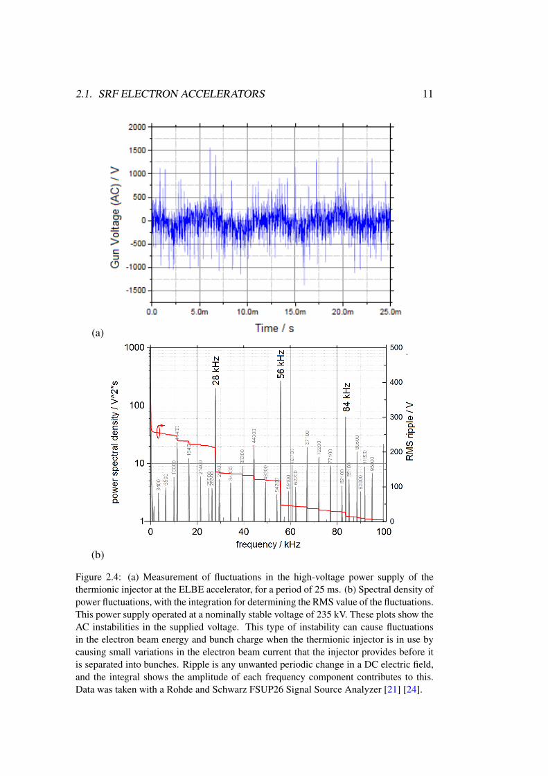
Instabilities in beam and/or bunch parameters, such as bunch charge or beam en-ergy, can be the source of noise in the various secondary sources driven by theelectron beam. There are many possible origins for these instabilities and it canbe difficult because of this to determine the exact causes. Some types of instabili-ties can originate in the injector. In the case of the thermionic injector, for exam-ple, instabilities in the buncher can cause variations in the bunch charge. Otherinstabilities, such as beam energy, can be caused by changes in, for instance, thephase or amplitude of the accelerating field in the RF cavities. Figure 2.4 showsa measurement of the stability of the high voltage power source that drives thethermionic injector at ELBE [21]. This power supply provides high-voltage DCat 235 kV to the thermionic injector which is used to pull electrons from a bar-ium cathode (CPI EIMAC Y-845 Dispenser Cathode Assembly [22]) [23]. Theobserved changes in this voltage can cause changes in the current of the electronbeam provided to the buncher, which could affect the bunch charge. Beam energyis also likely affected, but because of the small relative change (±500 V in a 235kV DC potential, or about 0.2%) any possible instabilities would be difficult todetect [24]. Bunch charge fluctuations lead to intensity instabilities in the super-radiant THz sources. Instabilities in the beam energy would, among other things,affect the superradiant THz spectrum (e.g. the center frequency of the undulatorradiation). As part of this work a pulse-resolved intensity measurement has beendeveloped that allows for correction of intensity instabilities.


(a)

(b)

Figure 2.4: (a) Measurement of fluctuations in the high-voltage power supply of thethermionic injector at the ELBE accelerator, for a period of 25 ms. (b) Spectral density ofpower fluctuations, with the integration for determining the RMS value of the fluctuations.This power supply operated at a nominally stable voltage of 235 kV. These plots show theAC instabilities in the supplied voltage. This type of instability can cause fluctuationsin the electron beam energy and bunch charge when the thermionic injector is in use bycausing small variations in the electron beam current that the injector provides before itis separated into bunches. Ripple is any unwanted periodic change in a DC electric field,and the integral shows the amplitude of each frequency component contributes to this.Data was taken with a Rohde and Schwarz FSUP26 Signal Source Analyzer [21] [24].


Arrivaltime

The arrivaltime of radiation pulses is a critical value to know for the time-resolvedexperiments in this work. It is important to keep in mind, then, that acceleratordriven radiation sources suffer from arrivaltime instabilities that make it difficultto perform time-resolved measurements without first accounting for this. One dif-ferentiates between two timescales of the instability here, to be known from hereon as jitter and drift. Jitter is defined as pulse-to-pulse changes in arrivaltime ontimescales of less than 1 second. Drift is defined as variations on longer timescales of more than 1 second. Currently the jitter at ELBE is in the few picose-donds (ps) (FWHM) range, and the drift over long periods of a day or more is onthe few 10 ps (FWHM) range. One possible source of this type of instability is theactual arrivaltime of the electron bunch. If there are any instabilities in the timingsystem used to inject the electrons it would show up as this type of jitter. Jitterthat is present at this point will be present at every location downstream in theaccelerator. After that there are the instabilities in the RF sources, which are ei-ther klystrons or, in newer generations of machines such as the ELBE, solid-stateRF sources [25]. Changes in phase of the accelerating field within the acceler-ator cavities lead to fluctuations in beam energy. Fluctuations in beam energycan translate into arrivaltime differences in all dispersive elements of the accel-erator. Finally, changes in temperature and humidity can affect how accuratelythe timing and clock signal is distributed to external systems, such as the laserswhich are used in the TELBE lab. Any jitter between these external systems andthe accelerator master clock will also show up as timing jitter in any experimentwhich involves both of those systems working in concert. As a part of this work,a pulse-resolved arrivaltime monitor has been developed to measure and correctthe arrivaltime value on a timescale of 30 fs (FWHM).

Beam position

Changes in the position of the electron bunches within the accelerator can becaused by instabilities of the magnetic fields in various beamline components,such as sleeves, dipole, or quadrupole magnets. Instabilities in beam position canaffect the performance of certain secondary radiation sources, such as the diffrac-tion radiator, of the TELBE facility. Figure 2.5 shows the spectral components ofa measurement of beam position jitter in the ELBE accelerator. The measurementwas taken at a position between the two main accelerator modules with the beamat this point having an energy of 12 MeV. The detector was a commercial beamposition monitor from Libera, called the Spark [26]. The data was taken on indi-vidual bunches at 400 Hz, with the beam having a repetition rate of 1.625 MHz.The beam was shown to move more in the x direction, with a movement FWHM


of 149.4 µm as compared to a movement FWHM of 51.4 µm in the y direction.Beam position shifts may result in an increase in intensity from the diffraction ra-diator source, due to the emission of transition radiation [27] caused by electronsimpinging on the diffraction screen. This causes an observable increase in overallintensity and high-frequency spectral content.

Figure 2.5: Spectrum of beam position changes measured at ELBE with a Libera Sparkbeam position monitor positioned between the two main accelerating modules of the ac-celerator. The top plot shows the changes in the horizontal position, with an FWHM of149.4 µm, and the bottom plot shows the vertical jitter, with a FWHM of 51.4 µm jitter.Data taken with a beam energy of 12 MeV (total beam energy was 34 MeV, but data wastaken after only the first accelerator module so the beam measured was at 12 MeV), bunchcharge of 46 pC, using the thermionic injector, at a repetition rate of 1.625 MHz [28].


2.2 Superradiant THz sources

2.2.1 Superradiant principleThe superradiant principle states that the intensity of radiation from emitters in-creases as the square of the number of emitters, I ∝ (number of emitters)2, forcertain cases. The requirement is that the area the emitters radiate from must besufficiently small compared to the wavelength of the emitted radiation [29]. Forexample, a bunch of electrons emitting in phase less than 300 microns from eachother will have extremely enhanced emissions for wavelengths below 1 THz. Thiscan be described as shown:

Wbunch =[(1− f)Nelectron + fN2

electron

]Welectron (2.2)

where N is the number of emitters (in this case electrons),Welectron is the emissionof a single electron, and f is known as the formfactor, here shown for an electronbunch with a Gaussian density distribution:

f(ν) = e−0.5(2πν)2( τ

2.35)2 (2.3)

where ν is the wavelength and τ is the FWHM (full width half max) of the bunchdensity distribution. This basic principle is what allows electron accelerator drivenlight sources to act as high-intensity, high repetition rate light sources given theelectron bunches can be compressed to sufficiently short durations [6]. Oncethe bunches are short and highly charged any radiator type can be utilized, andhence an enormous variety of pulse forms can be generated. An illustration of thechanges to the formfactor for various electron bunch lengths is shown in Figure2.6.

2.2.2 Radiator typesTransition Radiation

Transition radiation was first theoretically described by V. L. Ginzburg and I.Frank in 1945 [30]. This is the radiation that is emitted when a charged particletravels between two materials with differing dielectric constants. The followingequation analytically describes the intensity distribution of transition radiation ona detector screen:

d2U

dωdΩ=

e2

4π3ε0c· β2 sin2 θ

(1− β2 cos2 θ)2(2.4)

where e is electron charge, ε0 is the dielectric constant in vacuum, β is the ratioof the speed of a particle to the speed of light (β = v

c), and θ is the angle from the

2.2. SUPERRADIANT THZ SOURCES 15

Figure 2.6: Superradiant emission from electron bunches becomes significant for frequen-cies sufficiently lower than the inverse of the bunch duration τ . Following equation 2.2 theemission scales quadratically with the charge at low enough frequencies but diminishes athigher frequencies when a smaller fraction of the charge fits within the wavelength. Thisbehavior can be described by the dimensionless form factor f. (a) Form factors plottedfor an assumed Gaussian bunch form with duration (FWHM) of 3000 fs (FWHM), 300 fs(FWHM) and 30 fs (FWHM) (grey-shaded). (b) Corresponding dependence of the pulseenergies at THz frequencies of 0.3 THz (black solid), 1 THz (red-dashed), 2 THz (blue-dotted) and 3 THz (green-dash-dot) on the bunch charge. For simplicity a “white” radiatorwith a frequency independent emission characteristic is assumed. The upper edge of theblue-shaded area corresponds to the case of a form factor equal to 1. Taken from [6].

source to a point on the detector, Ω is the solid angle of the detector, ω is angularfrequency, and U is pulse energy. Specifically, Equation 2.4 gives the intensitydistribution of the radiation emitted by a single electron passing from vacuuminto an infinite metal sheet that is perpendicular to the path of the electron, with anexample of the result in Figure 2.7. The electric field of the particle changes whenthe dielectric constant changes, and the difference is “shaken off” as transitionradiation. This equation includes only a first order approximation for the distancebetween the emitting screen and the detector, which means so-called “near-field”radiation is neglected, so this is only valid in the far field. The intensity of theradiation emitted is proportional to log(γ) of the particle, which sparked interest intransition radiation as a tool to measure relativistic particle energies [6]. Equation2.4 makes several assumptions which should be addressed. It describes an infinitemetal plane, it shows the intensity distribution from a single electron, and it isonly valid for the far field. The far field condition is D > γ2λ, where D is thedistance, γ is the electron energy, and λ is the wavelength. The far-field distance


Figure 2.7: Illustration of calculated transition radiation distribution from an infinitescreen on a far-field detector. a) A cross section of the intensity distribution across thedetector, showing the result calculated by the Ginzburg-Frank equation. b) a 3D represen-tation of the intensity distribution, showing the donut-shaped intensity distribution on thedetector, which is given by taking the Gizburg-Frank result and applying it to the entiredetector surface. Adapted from TESLA Report 2005 [27]

described is wavelength dependent. The limit comes from the Fresnel diffractionequations, and is essentially defining where only the first term is contributing. Toaccount for electrons in bunches, instead of single electrons, one can introducethe formfactor term mentioned earlier. This still does not solve the problem ofa single electron emitting up to infinitely high frequencies, as this is clearly notphysical. The upper limit is generally defined by the plasma frequency of themetal the radiator is made from. One can ignore this in this work because theplasma frequencies are generally in the infrared, which is far higher than it ispossible to radiate with the moderately short electron bunches at TELBE. Onecan account for a finite metal radiator by using a numerically solvable equationthat can be derived with the virtual-photon method [31]. The parameterizationused in the following equations is shown in Figure 2.8.

The first step gives up an equation which, when the radiator radius approachesinfinity, returns the Ginzburg-Frank equation. This is known as the modifiedGinzburg-Frank Equation [27]:

d2U

dωdΩ=

e2

4πε0c· β2 sin2 θ

(1− β2 cos2 θ)2[1− T (θ, ω)]2 (2.5)

where T (θ, ω) is the correction factor which addresses the finite radiator, writtenin terms of θ and ω:

T (θ, ω) =ωa

cβγJ0

(ωa sin θ

c

)K1

(ωa

cβγ

)+

ωa

cβ2γ2 sin θJ1

(ωa sin θ

c

)K0

(ωa

cβγ

)(2.6)


Figure 2.8: Schematic showing the parametrization used in the differential equations cal-culating diffraction radiation. This diagram illustrates the meaning of the various param-eters used in the Ginzburg-Frank equation, with Q(ρ, φ, 0) representing the coordinate onthe source screen in radial coordinates, and P (x, 0, D) being the radial coordinate on thedetector. In both cases the 0 is the height coordinate, making them two-dimensional. D isthe distance between the centers of the source and the detector, R is the distance betweenthe center of the source and an arbitrary point on the detector, and R′ is the distance be-tween an arbitrary point on the source and an arbitrary point on the detector. Taken from[27]

In these equations e is electron charge, ε0 is the permittivity of vacuum, c is thespeed of light, β is the ratio of electron speed to c, θ is the angle from the center ofthe radiator to the observation point on the detector, ω is the wavenumber, γ is theLorentz factor of the electron, a is the radius of the metal radiator, J0 and J1 areBessel functions of the first kind, and K0 and K1 are modified Bessel functions.To check the validity of this equation one can increase the radius a to the limit ofinfinity. For this case the terms in the correction factor are:

lima→∞

T (θ, ω) = 1J0

(ωa sin θ

c

)K1

(ωa

cβγ

)= 0 (2.7)

lima→∞

J1

(ωa sin θ

c

)K0

(ωa

cβγ

)= 0 (2.8)

On the other end of the spectrum, an infinitely small radiator, one would expect tohave no radiation. In this case:

lima→0

T (θ, ω) = 1 (2.9)


which shows there is nothing radiated in this case.At this point the equation describes the spectral density of DR radiation on

a given point on a screen some distance away from the source, but is only validwhere the far-field condition given earlier is still true. In order to get an equationthat works in near-field as well one needs to revisit the derivation of this equation,which uses a first order approximation of the distance between the radiator andthe detector. If a second order approximation is used, the far-field condition isno longer required to get a good solution, but it becomes unsolvable by analyticmeans, so a numerical calculation must be utilized. The distance R′ from anarbitrary spot on the radiator to an arbitrary spot on the detector is:

R′ =√D2 + (x− ρ cosφ)2 + (ρ sinφ)2 ≈ R− xρ cosφ

R+ρ2

2R(2.10)

R is the distance from the center to the diffraction source to the center of thedetector, ρ is the radius of an arbitrary point on the diffraction radiator, φ is theazimuthal angle to the point on the diffraction radiator, and x is the point on thedetector. Taking the three terms shown, one can derive the following equation forthe spectral density. This equation leaves off the scaling factor, but is otherwise amore accurate version of Eq. 2.5 above.

d2U

dωdΩ∝∣∣∣∣∣∫ a

0J1(kρ sin θ)K1

(kρ

βγ

)exp

(ikρ2

2R

)ρdρ

∣∣∣∣∣ (2.11)

Taking the first order approximation of Eq. 2.11 and performing the integrationon it yields the original Ginzburg-Frank.

Diffraction Radiation

Diffraction radiation is generated when an electron bunch passes near, but notthrough, a conducting material. This is usually accomplished by taking a transi-tion radiation source and inserting a small aperture which the charged particlescan pass through, making a so-called diffraction radiator. This is illustrated inFigure 2.9. The electric field still experiences a change in dielectric constant evenif the particle itself does not pass directly through the material. It is very similarto transition radiation in both the procedure to generate it and the pulse character-istics. The main difference is a loss of some of the higher frequency componentswhich is dependent on the aperture size, with larger apertures losing more higherfrequency components than screens with smaller apertures.

From a calculation standpoint it is possible to get the intensity distribution bystarting with the diffraction radiation equation, and subtracting out the contribu-tion of a small disc of metal in the center, in what will become the aperture. This


Figure 2.9: Working principle of a diffraction radiator (DR) and a simulated beam profilefor the horizontal polarization component. Left: This image is a diagram of the diffractionradiator installed at ELBE, with the grey truncated circle in the center being the screenitself. The lighter grey support structure surrounding it is used to adjust the position andangle of the screen in relation to the incoming electron beam, which is shown as a greenline passing through the aperture in the middle of the screen. The resulting radially po-larized THz pulse is shown in red. Right: A simulated diffraction radiation pulse profile,shown after polarization. The two lobes are the horizontally polarized portion of the radi-ally polarized original pulse. Taken from [6]

gives an equation which looks like this:

d2U

dωdΩ=

e2

4πε0c· β2 sin2 θ

(1− β2 cos2 θ)2[Tb(θ, ω)− Ta(θ, ω)]2 (2.12)

Ta(θ, ω) =ωa

cβγJ0

(ωa sin θ

c

)K1

(ωa

cβγ

)+

ωa

cβ2γ2 sin θJ1

(ωa sin θ

c

)K0

(ωa

cβγ

)(2.13)

Tb(θ, ω) =ωb

cβγJ0

(ωb sin θ

c

)K1

(ωb

cβγ

)+

ωb

cβ2γ2 sin θJ1

(ωb sin θ

c

)K0

(ωb

cβγ

)(2.14)

The variables are the same as in equation 2.5, with the addition that a is theradius of the screen, and b is the radius of the aperture in the screen. The modifiedGinzburg-Frank can be recovered if one takes the limit as a→∞ and the limit asb→ 0.


Figure 2.10: Illustration of the concept behind undulator radiation, showing the radiationas coming from a point source in the center of the undulator (left) and a calculation ofthe intensity distribution of a 1 THz tuned undulator in the fundamental frequency, whichshares a characteristic bell shape with higher odd numbered harmonics (right) Taken from[6].

Undulators

The principles of the undulator were described by V. L. Ginzburg in 1947 [32]. Itis a device based on synchrotron radiation, which was observed for the first timethat same year, at the General Electron Synchrotron accelerator [33]. The firstundulator was constructed by H. Motz in 1952 [34] at Stanford University. Byplacing multiple bending magnets in a row in order to create a sinusoidal beampath for a charged particle (shown in Figure 2.10) it is possible to create a narrowbandwidth, high intensity light source that can be tuned to range of frequencieswhich are set by the physical characteristics of the undulator and the electronbunch properties of the accelerator that powers it. The wavelength of undulatorradiation can be controlled by varying the strength of the magnetic field and theintensity by the energy and charge of the electron bunches passing through it. Theoutput wavelength is

λ =λu2γ2

(1 +

K2

2+ γ2θ2

)(2.15)

where λu is the undulator period length, γ is the electron energy, θ is the outputangle, K is the K-parameter (see 2.17). The bandwidth is given by ∆ν = 1/Nwhere N is the number of periods [35].

2.3. THZ RADIATION DETECTION 21

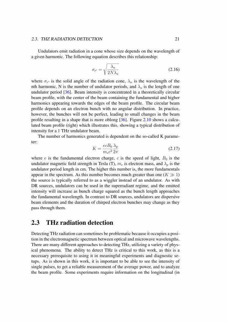
Undulators emit radiation in a cone whose size depends on the wavelength ofa given harmonic. The following equation describes this relationship:

σr′ =

√λn

2Nλu(2.16)

where σr′ is the solid angle of the radiation cone, λn is the wavelength of thenth harmonic, N is the number of undulator periods, and λu is the length of oneundulator period [36]. Beam intensity is concentrated in a theoretically circularbeam profile, with the center of the beam containing the fundamental and higherharmonics appearing towards the edges of the beam profile. The circular beamprofile depends on an electron bunch with no angular distribution. In practice,however, the bunches will not be perfect, leading to small changes in the beamprofile resulting in a shape that is more oblong [36]. Figure 2.10 shows a calcu-lated beam profile (right) which illustrates this, showing a typical distribution ofintensity for a 1 THz undulator beam.

The number of harmonics generated is dependent on the so-called K parame-ter:

K =ecB0

mec2λp2π

(2.17)

where e is the fundamental electron charge, c is the speed of light, B0 is theundulator magnetic field strength in Tesla (T), me is electron mass, and λp is theundulator period length in cm. The higher this number is, the more fundamentalsappear in the spectrum. As this number becomes much greater than one (K 1)the source is typically referred to as a wiggler instead of an undulator. As withDR sources, undulators can be used in the superradiant regime, and the emittedintensity will increase as bunch charge squared as the bunch length approachesthe fundamental wavelength. In contrast to DR sources, undulators are dispersivebeam elements and the duration of chirped electron bunches may change as theypass through them.

2.3 THz radiation detectionDetecting THz radiation can sometimes be problematic because it occupies a posi-tion in the electromagnetic spectrum between optical and microwave wavelengths.There are many different approaches to detecting THz, utilizing a variety of phys-ical phenomena. The ability to detect THz is critical to this work, as this is anecessary prerequisite to using it in meaningful experiments and diagnostic se-tups. As is shown in this work, it is important to be able to see the intensity ofsingle pulses, to get a reliable measurement of the average power, and to analyzethe beam profile. Some experiments require information on the longitudinal (in


the time domain) shape of individual pulses, or even their actual waveform. Thefollowing sections deal with the different THz detection schemes and detectorsutilized at TELBE to characterize the TELBE THz radiation.

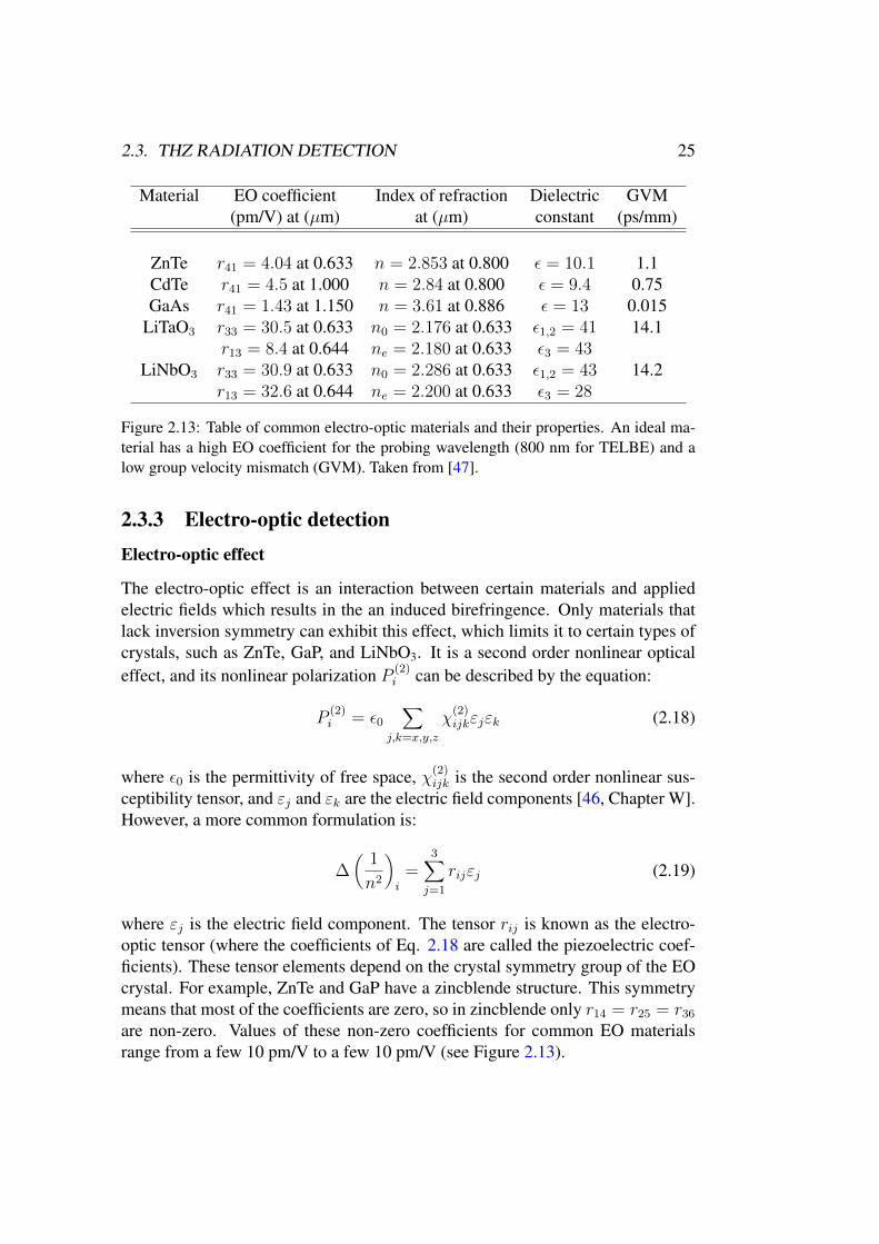
2.3.1 Pyroelectric detectorsThe pyroelectric effect is a phenomenon that occurs when so called pyroelectricmaterials change temperature. The earliest mention of this effect comes from the3rd century BC by a Greek named Theophrasutus [37]. He noted that tourma-line would attract ash or small bits of metal when heated. The effect was laterrediscovered in the 18th century, and finally named in 1824 by David Brewster[38]. Changes in temperature cause a change of the electrical polarization whichinduces a voltage across the material [39]. This voltage then gradually decreasesdue to leakage current, either through the material itself or through an outside path.Pyroelectric materials can therefore be used to detect radiation from the THz tox-ray range by measuring voltage across them. Any change in voltage is causedby heat being deposited in the material by a light pulse. Thus, the appearanceof a detected light pulse is two spikes in voltage, of opposite polarity. The firstspike appears when the material is warmed by the light pulse, the second spike iscaused when the material cools back to its original temperature after the pulse haspassed, while a continuous radiation beam would not lead to a detectable signal.Front end electronics have been developed at DESY that take these two pulses andoutput them as a single pulse to make analyzing the detected pulses easier [40]. Adiagram of a basic pyroelectric detector is given in Figure 2.11.

Pyrodetectors work at room temperature and can be operated at repetition ratesin the 100 kHz regime. This type of detector has been most frequently used atTELBE to date because it allows pulse to pulse intensity detection at the typicaloperating repetition rate of 100 kHz. It is also easy to convert the signal to a quan-titative measure of the pulse energy because the intensity response is linear. Thereare a few major problems, though, with this type of detector. The frequencies ofinterest in THz are generally difficult to absorb with the standard materials used inpyroelectric detectors. These materials can be transparent to some frequencies inthe THz range which of course make it difficult to detect them. Any frequenciesthat pass through the absorber material are not measured in the detector, leadingto possibly lower readings than the actual beam power. There is also a problemwith linearity at high intensities. The special fast detectors that were developed atDESY have a linear response up to a signal value of 1 V, so it is important to limitincoming intensity so that the signal is less than 1 V in order to stay in the linearregime. In addition the base noise level is high (±50 mV). This leads to a largeerror bar in the few 10% range in single pulse intensity measurements. Finally,pyroelectric detectors are too slow to resolve the actual pulse duration, which is


Figure 2.11: Diagram of a pyroelectric detector. Φ(s)t is the incoming light pulse, dp isthe thickness of the pyroelectric material, As is the surface area of the radiation sensitiveelement (where the pyroelectric material is between the two electrodes) which has someabsorption factor dependent on the incoming wavelength. The output signal voltage is µ′sand the noise voltage is µ′r. Taken from [41].

in the few ps (FWHM) regime.

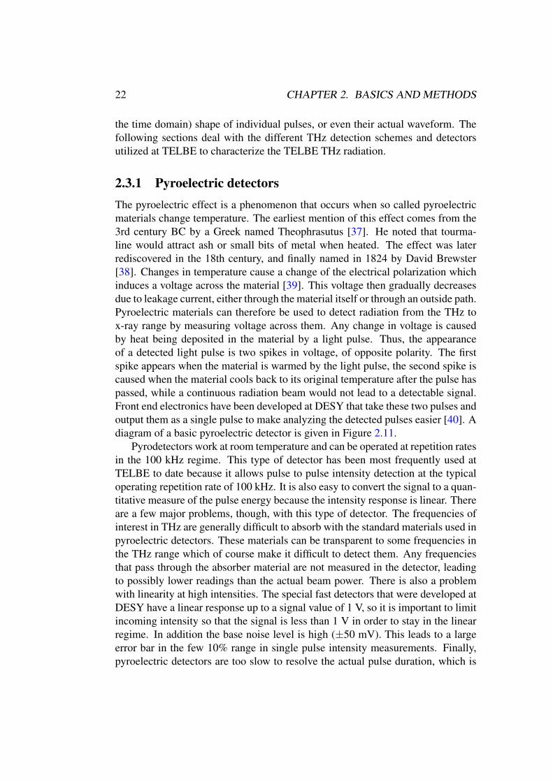
2.3.2 Schottky DiodeSchottky diodes are diodes formed with a metal-semiconductor junction, as op-posed to the semiconductor-semiconductor junction that regular diodes use. Schot-tky diodes have a lower turn-on voltage, which is the voltage needed to allowcurrent to flow through, and a faster response time than either regular diodes orpyroelectric detectors, with a bandwidth in the GHz range [42]. These detectorswork by rectifying and demodulating signals, converting them into a DC voltage.Like pyroelectric detectors, they can be used as broadband detectors, or tuned tospecific wavelengths with varying bandwidths by coupling them with different,carefully designed antennas [43]. Because of the small size and simplicity of con-struction, it is possible to mount several detectors with different antennas on asingle chip, creating a single-chip spectrometer. Because of the speed of the de-tectors, higher repetition rates into the tens of MHz range can be utilized whilemaintaining single-pulse measurement capability [44]. One such spectrometer isbeing developed under the BMBF project InSEL and an early version is shown inFigure 2.12 [45]. However, Schottky diode detectors remain too slow to measurethe actual pulse form of a ps-range THz pulse.


(a)

(b)

Figure 2.12: (a) Integrated on-chip THz detector with patch antenna, Schottky diode,matching, biasing and read-out circuitry in a coplanar waveguide layout. (b) Chip photo-graph of THz detector manufactured in UMS BES GaAs process. [44]


Material EO coefficient Index of refraction Dielectric GVM(pm/V) at (µm) at (µm) constant (ps/mm)

ZnTe r41 = 4.04 at 0.633 n = 2.853 at 0.800 ε = 10.1 1.1CdTe r41 = 4.5 at 1.000 n = 2.84 at 0.800 ε = 9.4 0.75GaAs r41 = 1.43 at 1.150 n = 3.61 at 0.886 ε = 13 0.015

LiTaO3 r33 = 30.5 at 0.633 n0 = 2.176 at 0.633 ε1,2 = 41 14.1r13 = 8.4 at 0.644 ne = 2.180 at 0.633 ε3 = 43

LiNbO3 r33 = 30.9 at 0.633 n0 = 2.286 at 0.633 ε1,2 = 43 14.2r13 = 32.6 at 0.644 ne = 2.200 at 0.633 ε3 = 28

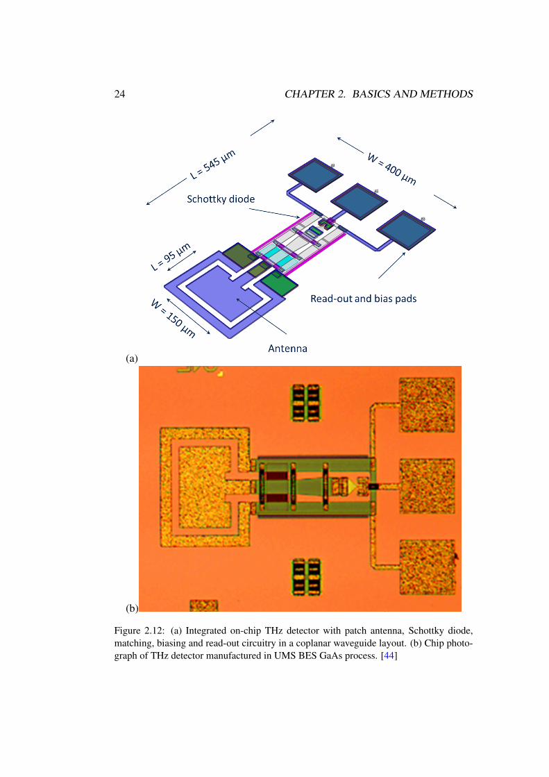
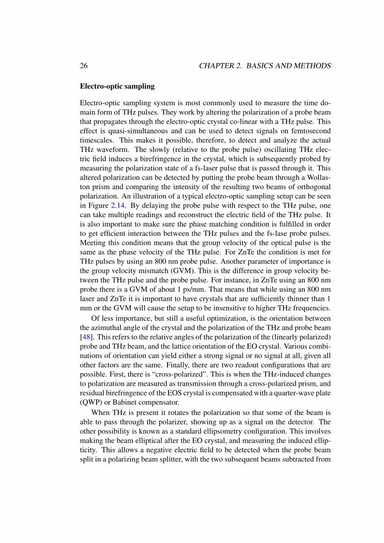
Figure 2.13: Table of common electro-optic materials and their properties. An ideal ma-terial has a high EO coefficient for the probing wavelength (800 nm for TELBE) and alow group velocity mismatch (GVM). Taken from [47].

2.3.3 Electro-optic detectionElectro-optic effect

The electro-optic effect is an interaction between certain materials and appliedelectric fields which results in the an induced birefringence. Only materials thatlack inversion symmetry can exhibit this effect, which limits it to certain types ofcrystals, such as ZnTe, GaP, and LiNbO3. It is a second order nonlinear opticaleffect, and its nonlinear polarization P (2)

i can be described by the equation:

P(2)i = ε0

∑j,k=x,y,z

χ(2)ijkεjεk (2.18)

where ε0 is the permittivity of free space, χ(2)ijk is the second order nonlinear sus-

ceptibility tensor, and εj and εk are the electric field components [46, Chapter W].However, a more common formulation is:

∆(

1

n2

)i

=3∑j=1

rijεj (2.19)

where εj is the electric field component. The tensor rij is known as the electro-optic tensor (where the coefficients of Eq. 2.18 are called the piezoelectric coef-ficients). These tensor elements depend on the crystal symmetry group of the EOcrystal. For example, ZnTe and GaP have a zincblende structure. This symmetrymeans that most of the coefficients are zero, so in zincblende only r14 = r25 = r36are non-zero. Values of these non-zero coefficients for common EO materialsrange from a few 10 pm/V to a few 10 pm/V (see Figure 2.13).


Electro-optic sampling

Electro-optic sampling system is most commonly used to measure the time do-main form of THz pulses. They work by altering the polarization of a probe beamthat propagates through the electro-optic crystal co-linear with a THz pulse. Thiseffect is quasi-simultaneous and can be used to detect signals on femtosecondtimescales. This makes it possible, therefore, to detect and analyze the actualTHz waveform. The slowly (relative to the probe pulse) oscillating THz elec-tric field induces a birefringence in the crystal, which is subsequently probed bymeasuring the polarization state of a fs-laser pulse that is passed through it. Thisaltered polarization can be detected by putting the probe beam through a Wollas-ton prism and comparing the intensity of the resulting two beams of orthogonalpolarization. An illustration of a typical electro-optic sampling setup can be seenin Figure 2.14. By delaying the probe pulse with respect to the THz pulse, onecan take multiple readings and reconstruct the electric field of the THz pulse. Itis also important to make sure the phase matching condition is fulfilled in orderto get efficient interaction between the THz pulses and the fs-lase probe pulses.Meeting this condition means that the group velocity of the optical pulse is thesame as the phase velocity of the THz pulse. For ZnTe the condition is met forTHz pulses by using an 800 nm probe pulse. Another parameter of importance isthe group velocity mismatch (GVM). This is the difference in group velocity be-tween the THz pulse and the probe pulse. For instance, in ZnTe using an 800 nmprobe there is a GVM of about 1 ps/mm. That means that while using an 800 nmlaser and ZnTe it is important to have crystals that are sufficiently thinner than 1mm or the GVM will cause the setup to be insensitive to higher THz frequencies.

Of less importance, but still a useful optimization, is the orientation betweenthe azimuthal angle of the crystal and the polarization of the THz and probe beam[48]. This refers to the relative angles of the polarization of the (linearly polarized)probe and THz beam, and the lattice orientation of the EO crystal. Various combi-nations of orientation can yield either a strong signal or no signal at all, given allother factors are the same. Finally, there are two readout configurations that arepossible. First, there is “cross-polarized”. This is when the THz-induced changesto polarization are measured as transmission through a cross-polarized prism, andresidual birefringence of the EOS crystal is compensated with a quarter-wave plate(QWP) or Babinet compensator.

When THz is present it rotates the polarization so that some of the beam isable to pass through the polarizer, showing up as a signal on the detector. Theother possibility is known as a standard ellipsometry configuration. This involvesmaking the beam elliptical after the EO crystal, and measuring the induced ellip-ticity. This allows a negative electric field to be detected when the probe beamsplit in a polarizing beam splitter, with the two subsequent beams subtracted from


each other. The response here is linear with electric field, showing all positiveand negative components at the final readout. While electro-optic sampling in thisconfiguration is fast enough to detect the longitudinal pulse profile, and even thewaveform, it is still necessary to integrate over many pulses.

Figure 2.14: Electro-optic sampling setup. The THz pulse is focused onto an electro-optic crystal, ZnTe in this example, with an off-axis parabola. The probe laser is passedcollinearly through the same spot on the crystal. A quarter waveplate (λ/4) is then usedto adjust for any changes to the probe beam caused by the dispersion of the electro-opticcrystal. The probe beam is then analyzed by passing it through a polarizing beam splitter(PBS), and the two resulting beams are sent into two detectors (D1 and D2) where thesignals are subtracted (D1-D2) to get the final measurement of the THz pulse. Not shownis a mechanical delay stage to move the relative arrivaltime of the probe pulse to differentparts of the THz pulse in order to sample the whole pulse. Taken from [48].

Single shot THz detection

In addition to the basic EOS setup, which uses multiple THz pulses to create animage of the average pulse form, there are single shot methods which allow theimaging of a single THz pulse all at once. One such method, which is in use atTELBE, is called spectral decoding (or alternately spectral encoding) [49]. This isa method where a pulse from a fs-laser is taken and stretched, making the resultingpulse much longer temporally and with a linear spread of spectral components intime (which is referred to as a chirped pulse). Then this pulse is passed collinearlythrough an EO crystal with the THz. This results in the temporal profile of the THzpulse being transferred to the spectrum of the probe pulse. The resulting image ofthe THz pulse can then be read out by a line-array CCD coupled to a spectrometer,as illustrated in Figure 2.15. The temporal resolution of this setup depends onthe how far the pulse is stretched and the characteristics of the spectrometer andreadout camera.


Figure 2.15: Spectral decoding setup. A fs-laser pulse is passed through a stretcher,lengthening it to a multi-ps long pulse. It is then passed through a polarizer to eliminateany unwanted polarizations. Next it is sent through an electro-optic crystal collinear withthe THz pulse being measured. In this case, the THz pulse is generated by the samelaser, but in TELBE the THz would originate in the CDR or undulator. The laser pulseis once again passed through a polarizer, this time to remove the original polarization,leaving only the light that was rotated by the THz pulse. Finally, it is passed through aspectrometer and read by a CCD. This scheme was adapted to the requirements of theTELBE facility as part of this work. The setup is able to achieve a time resolution of 30fs (FWHM). It also allows the imaging of the waveform of individual THz pulses. Takenfrom [49].

2.3.4 PyroCam

Using the same physical process as the previously described pyroelectric detec-tors, a company called OPHIR produces a THz beam profiler named the PyroCam[50] that uses a 2D array of 80 µm sized pyroelectric detectors arranged as pixels.This camera can display beam profiles from the visible to the THz range for usein focusing and beam profiling. One drawback is the varying frequency response,as described earlier in the pyroelectric detector section. For longer wavelengthsin particular it is possible the PyroCam is insensitive, and the beam profile imagethat appears might only contain a subset of the frequencies, in this case higherTHz, that make up the beam. It is then possible that the spatial profile of the var-ious frequency components of a THz beam can differ, leading to beam profiles


that might not be accurate for the entire beam, or might show changes in profileor intensity for beams with different narrowband frequencies even when the beamshape itself has not changed.

2.3.5 Terahertz PowermeterAccurate measurements of beam power are problematic in the THz range [51].Ophir Optics manufactures a power sensor that is claimed to be calibrated for 0.3THz to 10 THz, making it a useful tool for the characterization of the TELBE THzbeams [52]. It consists of a thermopile detector utilizing a volume absorber madeof neutral density (ND) glass, which has a diameter of 12 mm. A thermopile is acollection of thermocouples (a metal-metal junction) connected in series, and eachthermocouple generates a current based on the thermoelectric effect, which itselfis caused by the electron energy levels in the two metals being shifted by differentamounts as the temperature changes [39]. The use of a volume absorber helpsto prevent too much power from depositing in a small volume (as in a surfaceabsorber) and damaging the sensor. Because the power measurement depends ondeposited heat, and that heat can take several seconds to dissipate, these power me-ters are most useful for measuring average power, not single pulse power. TELBEuses an Ophir Optics 3A-P-THz sensor, which has a range of 15 µW to 3 W, witha 4 µW noise level. The sensor is read out by an Ophir Optics Vega powermeter.The calibration has been verified by the Phyikalisch-Technische Bundesanstalt(PTB) for THz frequencies between 1 and 5 THz [51] as well as for 0.7 THz.

Chapter 3

Results

3.1 Diagnostic developmentsTELBE is the first working superradiant THz user facility driven by a quasi-cwSRF accelerator [6]. The primary application of TELBE in the materials and lifesciences is to utilize the transient THz fields as a novel highly selective excitationfor non-linear dynamics [3]. These dynamic processes are typically studied bymeans of pump-probe experiments on few 10 fs (FWHM) timescales involvingsynchronized external laser systems. The main motivation for the developmentspresented here is that ultrafast experiments at TELBE require a novel pulse re-solved diagnostic and data acquisition system in order to achieve the excellentdynamic range and time resolution required to probe the often subtle fingerprintsof the induced transient states of matter. This has to be done by correcting forfluctuations in the THz pulse parameters post-mortem, specifically arrivaltime andintensity, since the ELBE accelerator lacks suitable beam-based feedbacks.

This work yielded the development of two main diagnostic systems at TELBE,one prototype THz arrivaltime monitor capable of few 10 fs (FWHM) resolutionand one pulse-resolved intensity monitor. As shown later, the former has beenused in several successful time-resolved experiments performed at TELBE. Thelatter is still in the testing phase and has only been used in one example exper-iment, shown in section 3.3. Figure 3.1 shows the layout of the pulse-resolvedarrivaltime system and intensity monitor as well as two measurements taken ofthe arrivaltime and intensity fluctuations.

31

32 CHAPTER 3. RESULTS

(a)

(b) (c)

Figure 3.1: (a) Schematic diagram of the developed pulse-resolved diagnostic at theTELBE facility, combining a 30 fs (FWHM) resolution arrivaltime monitor with a pulseintensity monitor. (b) Arrival time of THz pulses over 1 second showing an arrivaltimejitter of around ±2 ps (FWHM). (c) Intensity of the THz pulses from the undulator tunedto 300 GHz taken over 1 second. Data taken using the thermionic injector, with a beamenergy of 24 MeV and a bunch charge of 70 pC. Adapted from [7].

3.1. DIAGNOSTIC DEVELOPMENTS 33

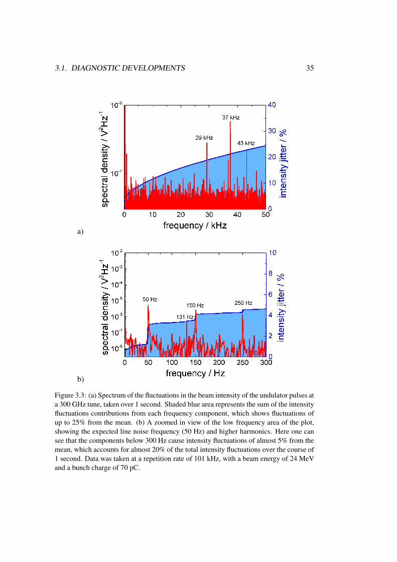
3.1.1 THz intensity instabilities and correctionOne of the challenges at TELBE is to account for changes in intensity of the THzpulses. Intensity measurements can be performed alongside the experiment, asshown in Figure 3.1 a. A wire grid polarizer is used as a beam splitter, and a smallportion of the THz beam acting as a pump excitation is diverted into a purpose-built pyroelectric detector. The most important factors for choosing the specificpyroelectric detector, developed at DESY for the TELBE intensity monitor, areits sufficiently high speed and robustness in handling (see Section 2.3.1 for moreinformation). These pyroelectric detectors have a relatively high noise floor of±50 mV [53]. One must also be careful not to put too much intensity onto thedetector. If the intensity is too high, the detector no longer has a linear response.In this specific case, the linear regime is when the output signal remains below 1V. Combined with the noise floor of ±50 mV this results in a relatively poor S/Nratio. Nevertheless, many revealing observations can be made. Figure 3.2 showsthat intensity fluctuations can be considerable and in the range of 50% or more.Figure 3.3 shows the spectral content of a typical pulse intensity measurement,taken over 1 second. Major frequencies are marked. A zoom in on the lower fre-quencies clearly shows 50 Hz (labeled in red), representing line noise, and manyhigher harmonics. A detailed discussion of the observed intensity instabilitiesfollows in section 3.1.2. Such an analysis can help in identifying the origin ofdifferent instabilities.

These instabilities can come from any number of sources, from fluctuationsin the bunch charge to beam position instabilities to electronic noise in the de-tection setup. Note that more than half of the intensity instabilities occur withfrequencies below 10 kHz (see Figure 3.3 a). This would allow for the employ-ment of moderately fast beam-based feedbacks to stabilize the intensity, giventhat the exact origins of the instabilities are known. In this work the determinationof the pulse-resolved intensity fluctuations serves to correct for them in exper-imental data. Moreover, these instabilities in pulse energy can be harnessed toprovide a pulse-energy-resolved measurement utilizing the intensity fluctuationsas fast modulation of the pulse intensity. One example of such a measurement isshown in section 3.3 where the fluence dependence of the THz-driven spinwaveis determined by including the pulse-resolved intensity measurement into the dataanalysis.


a)

b)

Figure 3.2: (a) Histogram of the change in intensity of pulses from the TELBE undulatorsource relative to the average intensity. (b) Histogram of the pulse-to-pulse (the change inarrivaltime compared to the previous pulse, rather than to an expectation value) intensityfluctuations taken over 1 second. Note that the uneven distribution here is likely causedby some of the THz pulses being intense enough to enter the non-linear regime of thedetector. Data was taken for an undulator tune of 300 GHz at a repetition rate of 101 kHz,with a beam energy of 24 MeV and a bunch charge of 70 pC.


a)

b)

Figure 3.3: (a) Spectrum of the fluctuations in the beam intensity of the undulator pulses ata 300 GHz tune, taken over 1 second. Shaded blue area represents the sum of the intensityfluctuations contributions from each frequency component, which shows fluctuations ofup to 25% from the mean. (b) A zoomed in view of the low frequency area of the plot,showing the expected line noise frequency (50 Hz) and higher harmonics. Here one cansee that the components below 300 Hz cause intensity fluctuations of almost 5% from themean, which accounts for almost 20% of the total intensity fluctuations over the course of1 second. Data was taken at a repetition rate of 101 kHz, with a beam energy of 24 MeVand a bunch charge of 70 pC.


3.1.2 THz arrivaltime instabilities and correctionAccurate timing of an accelerator to an external laser system can be accomplishedseveral ways. One method is based on RF pickups installed in the electron beampipe, and the signal caused by the Coulomb field of the passing bunch can beused to derive an arrival time with respect to an external laser [54]. One such sys-tem, called the beam arrivaltime monitor (BAM) has been installed between thediffraction radiator and the undulator sources of the TELBE facility. As shownlater in this work, the arrivaltime jitter determined here unfortunately does notcorrespond well to the arrivaltime jitter of the actual THz pulses in the TELBE lab-oratory. This rather surprising find made the development of an experiment-neararrivaltime monitor crucial. The monitor developed for TELBE is based on so-called spectral decoding, which is a single-shot electro-optic technique describedin detail in Section 2.3.3. Other techniques were considered, such as temporaldecoding [55] and spatial decoding [56]. These were ultimately found to be in-sufficient for TELBE. Temporal decoding maps time into spatial coordinates viaa non-linear process [55]. This process demands a high pulse energy probe laserbe used, which are only commercially available with low repetition rates. Spa-tial decoding [56] maps time into spatial coordinates via a projection of the THzfield onto the probe laser profile. The achievable time window for this processat TELBE is 1-2 ps (FWHM). This window is too small for the typical temporaldrifts in the ELBE accelerator, which are in the few ps (FWHM) regime.

In contrast, spectral decoding can be performed with nJ probe laser pulseswith a sufficiently wide time window. The probe beam for the monitor is currentlyprovided by a commercial amplified laser system [57]. Operating at 202 kHz itprovides µJ pulse energies, which is orders of magnitude more than required forspectral decoding. In the work performed here, most of the intensity of the probelaser can hence be used for probing the THz-driven dynamics, as shown in Figure3.1.

The magnitude of the overall jitter on a 1 second timescale is on the order of1-2 ps (FWHM) (see Figure 3.4). The jitter from pulse to pulse is on the orderof 200 fs (FWHM). Figure 3.5 gives an example phase noise spectrum of the ar-rivaltime instabilities taken with the experiment-near THz arrivaltime monitor atTELBE. The data was taken at the same rate as the accelerator was operating,101 kHz, and therefore includes the arrivaltime information of every THz pulseduring this time period. Strong spectral components are marked with their fre-quencies, including the line frequency of 50 Hz and its higher harmonics. As inthe case of the intensity instabilities, the dominant jitter components stem fromlower frequencies below 10 kHz (see Figure 3.5).


(a)

(b)

Figure 3.4: (a) Histogram of the arrivaltime relative to the average value. (b) Histogramof the pulse-to-pulse arrivaltime jitter. Data taken at the full 101 kHz repetition rate of theaccelerator over 1 second, with a beam energy of 24 MeV and a bunch charge of 70 pC.


(a)

(b)

Figure 3.5: (a) Example of a typical phase noise spectrum of the arrivaltime jitter in thepulses from the CDR source. Shaded blue area represents the sum of the arrivaltime jittercontributions from each frequency component. (b) Zoomed in plot of (a) showing the lowfrequency components. The 50 Hz line noise is present, as well as some higher harmonics.The relatively large component at 150 Hz possibly originates in a beam position instabil-ity, as seen in Fig. 2.5. Low frequency components below 300 Hz contribute around 75%of the total timing jitter. Data taken at the full 101 kHz repetition rate of the acceleratorover 1 second, with a beam energy of 24 MeV and a bunch charge of 70 pC.


3.1.3 Laser instabilities and correctionTELBE uses a commercial fs Ti:sapphire laser system provided by Coherent Inc[58]. The system consists of a laser oscillator (Vitara) and a regenerative ampli-fier (RegA 9000 [57]). The repetition rate of the oscillator was chosen to be 78MHz to match the 6th harmonic of the master clock speed of the ELBE, whichis 13 MHz. This oscillator then provides the seed pulse for the amplifier, andthe amplifier provides the laser pulses used in any experiments, with a small por-tion of the beam diverted for use in the arrivaltime monitor. The laser amplifiersystem provides 800 nm wavelength pulses with a bandwidth of 10 nm, a 100 fs(FWHM) pulse duration, and pulse energies of up to 6 µJ. The typical repetitionrate value is 202 kHz and the specified power drift rate is less than 4% over onehour with a pulse to pulse energy stability of about 2% FWHM [57]. Synchro-nization between the laser system and the master clock of ELBE is accomplishedby a commercial system called Synchrolock-AP, also manufactured by Coherent,Inc [59]. Measurement of phase noise in the synchronization of this system withthe master clock showed a timing jitter of 423 fs (FWHM) [60].

The intensity instabilities are corrected, in part, by setting the laser systemrepetition rate to double the THz rate. This gives two laser pulses per THz pulse.One pulse is used to sample the THz, and the other pulse is not altered and acts asa reference. The two pulses are then subtracted from one another, removing anyshared intensity changes originating from the laser system. In this way drifts inthe laser intensity at time scales longer than 5 µs are removed. This also reducesthe FWHM of the intensity fluctuations in the final data by nearly a factor of 2[60]. An example of this is shown in Figure 3.6. The correction removes theslower laser instabilities.

Timing instabilities in the laser system are corrected for by the pulse-to-pulsedata analysis described earlier. The arrivaltime measurement provided by the ar-rivaltime monitor gives the relative arrivaltime between the THz and the probelaser, which includes thereby any laser system timing jitter. The laser arrivaltimejitter is not separable from the THz arrivaltime jitter inside the arrivaltime monitorand, accordingly, the phase noise frequencies detected also contain contributionsfrom the laser instability. This has to be taken into account when discussing thepotential origin of the phase-noise frequencies in the arrivaltime in Section 3.1.2.


(a)

(b)

Figure 3.6: (a) Example of the laser intensity fluctuations compensation scheme. Thisshows a set of 6 measured laser pulses with the laser operating at 202 kHz. The peaksmarked with an R are reference signals. These are unmodulated laser pulses that have notbeen affected by THz. The signals marked S are the signal pulses, which are modulatedby the THz pulses. To perform the laser intensity correction, every S pulse has the Rpulse that follows subtracted from it. (b) Calculation of the signal for corrected (red) anduncorrected (black dashed) data.


3.1.4 Benchmarking of the Pulse-ResolvedData Acquisition System

The developed monitor systems, in combination with the pulse-resolved data ac-quisition and data analysis (see Figure 3.7), shall eventually serve to enable worldclass, ultrafast THz pump-probe experiments. The two most important parame-ters to establish to this end are the achievable time resolution and dynamic range.Benchmarking these values is an important step to show TELBE to be compet-itive with laser-based THz experiments in measurement quality, while providingall the additional advantages of an accelerator-driven source, e.g. high repetitionrate, unique spectral density, and variable THz pulse form.

First, the benchmarking of the achievable time resolution shall be described.In early pump-probe experiments the time resolution was determined by the cross-correlation of the pump and probe pulse durations because the pump pulses werenot carrier envelope phase (CEP) stable [61]. At the low THz frequencies availablefrom TELBE the pump pulse duration is in the few ps (FWHM) regime, which in aclassical pump-probe experiment would require a relatively modest synchroniza-tion of only 1 to 2 ps (FWHM). In contrast, the THz pulses from TELBE, as wellas from most laser-based THz sources, are carrier-envelope phase (CEP) stable.This allows study of phenomena on sub-cycle timescales, which is an importantnew field in THz research [3]. The time resolution in these modern THz pump-probe experiments in this case is given solely by the duration of the probe laserpulses and the accuracy of the arrivaltime measurement. The current probe laserpulse duration is 100 fs (FWHM), but an eventual upgrade to shorter pulse dura-tion is already being discussed. It is therefore important to establish the timingaccuracy of the arrivaltime monitor on few 10 fs (FWHM) timescales.

In order to verify a time resolution in the few 10 fs (FWHM) regime, de-spite the currently available 100 fs (FWHM) probe pulse duration, two differentapproaches were chosen. First, the effect of shifting the CDR pulse arrivaltime,acting as a timing signal, against the temporal position of the electric field of theundulator pulses, as determined by sequential electro-optic sampling (EOS), wasexplored (see Figure 3.8). This was done by shifting the CDR pulses in time withan opto-mechanical delay stage. At each position of the stage, the electric fieldof the undulator pulses was measured using sequential EOS. The position in timeof the observed electric field was used as a time reference, and the changes in itsposition were recorded as the CDR pulse was delayed (see Figure 3.8 a). Theresulting shifts are shown in Figure 3.8 b. The thereby observed deviation fromthe expectation value is less than 30 fs (FWHM), as shown in Figure 3.8 c.

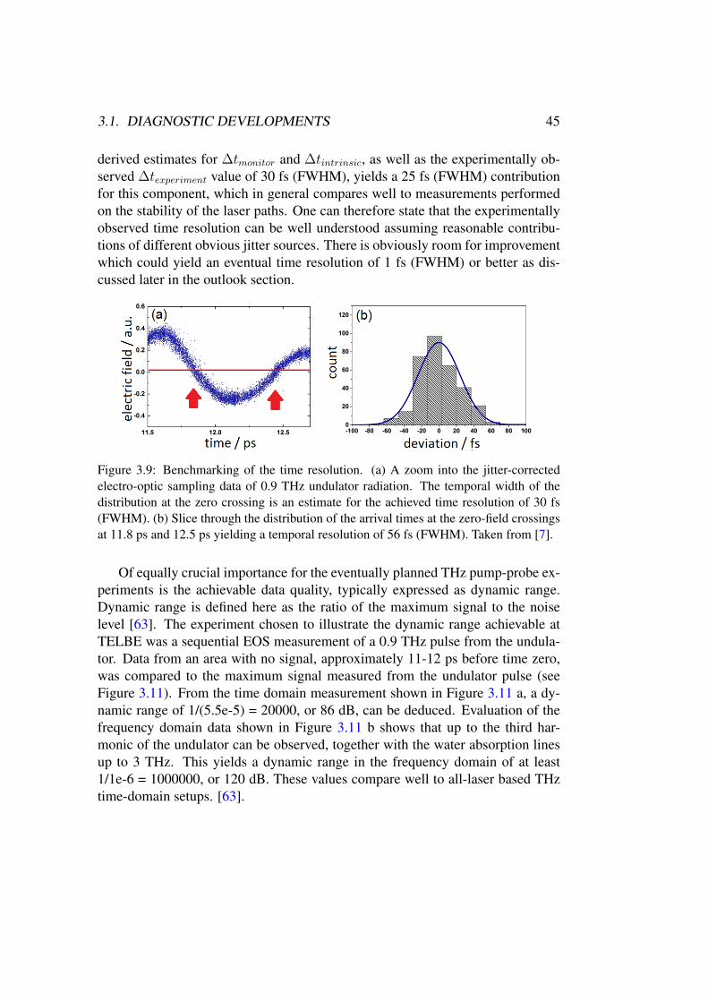
The second approach involves analyzing the arrivaltime-corrected data froma sequential EOS measurement of the electric field of a 0.9 THz undulator pulse(see Figure 3.9). The time-slice at the zero crossing is another representation of


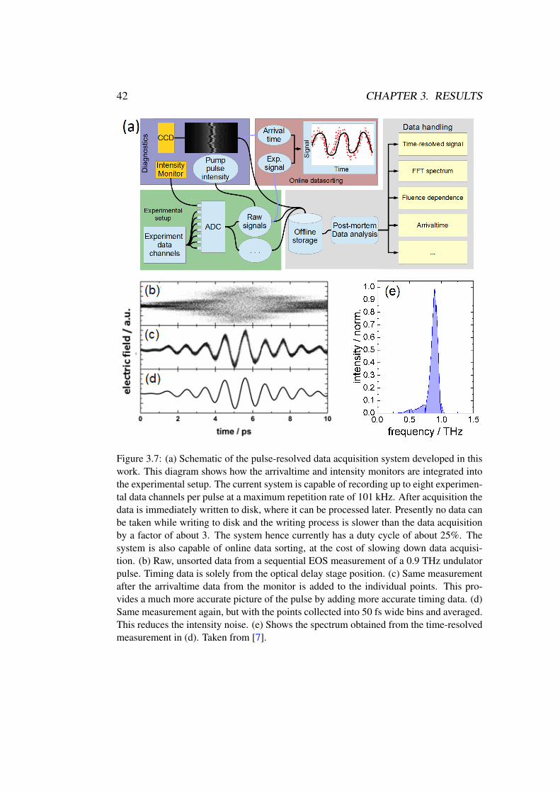
Figure 3.7: (a) Schematic of the pulse-resolved data acquisition system developed in thiswork. This diagram shows how the arrivaltime and intensity monitors are integrated intothe experimental setup. The current system is capable of recording up to eight experimen-tal data channels per pulse at a maximum repetition rate of 101 kHz. After acquisition thedata is immediately written to disk, where it can be processed later. Presently no data canbe taken while writing to disk and the writing process is slower than the data acquisitionby a factor of about 3. The system hence currently has a duty cycle of about 25%. Thesystem is also capable of online data sorting, at the cost of slowing down data acquisi-tion. (b) Raw, unsorted data from a sequential EOS measurement of a 0.9 THz undulatorpulse. Timing data is solely from the optical delay stage position. (c) Same measurementafter the arrivaltime data from the monitor is added to the individual points. This pro-vides a much more accurate picture of the pulse by adding more accurate timing data. (d)Same measurement again, but with the points collected into 50 fs wide bins and averaged.This reduces the intensity noise. (e) Shows the spectrum obtained from the time-resolvedmeasurement in (d). Taken from [7].


the accuracy of the timing correction. Assuming that intensity fluctuations can befully corrected or neglected, the time-slice distribution should also yield a valueof 30 fs (FWHM). A slightly large value of 50 fs (FHWM) is observed, likelybecause of contributions from intensity instabilities, as shown in Figure 3.9 b.

The experimentally established achievable time resolution of 30 fs (FWHM)is fully competitive with all-laser-based THz pump-probe setups. In the followingit shall be analyzed which individual contributions add up to this value to establishhow the time resolution can be further improved.

The limit for the intrinsic minimum timing accuracy ∆texperiment to be achievedby the arrivaltime monitor shown earlier in Figure 3.1 can be considered as a com-bination of discrete sources of jitter. Considered this way, the total experimentalminimum jitter is a combination of the intrinsic jitter between the undulator pulsesand the CD radiator ∆tintrinsic, the transport jitter arising from small instabilitiesin the separate optical paths in the monitor ∆ttransport, and the temporal resolutionof the utilized single shot EOS technique ∆tmonitor. This can be represented asthe following equation:

∆texperiment =(∆t2intrinsic + ∆t2transport + ∆t2monitor

)1/2(3.1)

where ∆texperiment is the minimum time resolution for the experiment. The intrin-sic jitter between the undulator pulses and the CD radiator is difficult to measuredirectly as detection of both pulses in the single shot EOS leads to strong interfer-ences. The thereby determined value of 58 fs (FWHM) [6] can hence only serveas an upper limit. However, another likely better estimate can be derived froman earlier experiment at the FLASH FEL which also combined two independentradiators, placed sequentially in a linear accelerator, in an ultra-fast pump-probeexperiment. In this case the first radiator was a VUV undulator, and the secondradiator was a superradiant THz undulator. THz streaking [62] allowed the deduc-tion of an intrinsic synchronization between the two radiators of 12 fs (FWHM)including several 10 meters of beam transport.

The temporal resolution of the single shot electro-optic sampling can be esti-mated from several factors. These are parameters such as the length of the chirpedlaser pulse, the characteristics of the spectrometer, and the pixel size of the readoutline camera. The setup at TELBE uses a pulse stretched to 8 ps (FWHM), and thespectrometer outputs a line just under 1 cm in length. Combined with a pixel sizeof 10 µm, this gives a final temporal resolution of the monitor of ∆tmonitor = 12 fs.Figure 3.10 a shows one method for obtaining an upper limit on the temporal res-olution of the monitor. The points from the zero-crossing of a 0.9 THz pulse aretaken and their line width analyzed. The calculated 56 fs (FWHM) distribution isan upper limit, likely broadened from the previously measured 30 fs (FWHM) byfluctuations in the electric field measurements. Figure 3.10 b shows four images


Figure 3.8: (a) Sketch of the scheme employed in THz pump laser probe experiment, withthe inset showing an example of the area of the THz pulse used to determine relative ar-rivaltime (b) Measured CDR pulse delay (red line) versus the observed temporal positionof the pulses from the undulator after arrivaltime correction. This establishes an uncer-tainty/jitter of less than 28 fs (FWHM) [7]. (c) Deviation between the expected value fromthe CDR delay position and the observed time shift of the undulator pulses. Taken from[6] [7].

from the arrivaltime detector of CDR pulses, taken 10 µs apart. Zooming in to thepeak shows the limit of the resolution of the arrivaltime monitor, which is 12 fs.

The final contributor to the experimentally observed jitter ∆ttransport stemsfrom the several meters long independent laser beampaths inside the TELBE lab-oratory. In the current setup the arrivaltime monitor and the experiment are on twoseparate laser tables at opposite corners of the laboratory. Assuming the earlier


derived estimates for ∆tmonitor and ∆tintrinsic, as well as the experimentally ob-served ∆texperiment value of 30 fs (FWHM), yields a 25 fs (FWHM) contributionfor this component, which in general compares well to measurements performedon the stability of the laser paths. One can therefore state that the experimentallyobserved time resolution can be well understood assuming reasonable contribu-tions of different obvious jitter sources. There is obviously room for improvementwhich could yield an eventual time resolution of 1 fs (FWHM) or better as dis-cussed later in the outlook section.

Figure 3.9: Benchmarking of the time resolution. (a) A zoom into the jitter-correctedelectro-optic sampling data of 0.9 THz undulator radiation. The temporal width of thedistribution at the zero crossing is an estimate for the achieved time resolution of 30 fs(FWHM). (b) Slice through the distribution of the arrival times at the zero-field crossingsat 11.8 ps and 12.5 ps yielding a temporal resolution of 56 fs (FWHM). Taken from [7].

Of equally crucial importance for the eventually planned THz pump-probe ex-periments is the achievable data quality, typically expressed as dynamic range.Dynamic range is defined here as the ratio of the maximum signal to the noiselevel [63]. The experiment chosen to illustrate the dynamic range achievable atTELBE was a sequential EOS measurement of a 0.9 THz pulse from the undula-tor. Data from an area with no signal, approximately 11-12 ps before time zero,was compared to the maximum signal measured from the undulator pulse (seeFigure 3.11). From the time domain measurement shown in Figure 3.11 a, a dy-namic range of 1/(5.5e-5) = 20000, or 86 dB, can be deduced. Evaluation of thefrequency domain data shown in Figure 3.11 b shows that up to the third har-monic of the undulator can be observed, together with the water absorption linesup to 3 THz. This yields a dynamic range in the frequency domain of at least1/1e-6 = 1000000, or 120 dB. These values compare well to all-laser based THztime-domain setups. [63].


Figure 3.10: (a) Four consecutive single-shot measurements of THz pulses from the co-herent diffraction radiator. (b) Magnified section around the signal maxima. They showthe temporal resolution of the spectral decoding setup resulting from the combination ofchirp, spectrometer characteristics, and pixel size of the readout camera. The repetitionrate in these measurements was 100 kHz. Taken from [7].


(a)

(b)

Figure 3.11: (a) Benchmarking the dynamic range in the time domain. THz-electro-opticmeasurement of the radiation emitted from the undulator source tuned to a frequency of0.9 THz (right) and a zoomed view of the 11-12 ps time interval before the temporaloverlap of the THz pump and laser probe (left). This time is sufficiently early to avoidinterference from artifacts due to reflections of the probe laser in the electro-optic crystal.This measurement gives a dynamic range of 4e8, or 86 dB, in the time domain. (b) Bench-marking the dynamic range in the frequency domain. Resulting THz frequency-domainspectrum when evaluating the full time-domain measurement over 120 ps on the left, andplotted on a logarithmic scale with water absorption spectrum on the right. Higher har-monics up to the 3rd order are observed. The measurement was performed in atmosphereand the narrow water absorption lines are clearly resolved up to 3 THz. The dashed whiteline represents the detection limit. This measurement thereby gives a dynamic range ofbetter than 1000000, or 120 dB, in the frequency domain. Taken from [7].


3.2 Characterization of TELBE sourcesThere are different fundamental characteristics of THz sources that make theminteresting candidates for studying linear and nonlinear THz-driven phenomena,namely the spectral content, beam profile, and intensity. Aside from these, theachievable stability and the achievable time resolution are also of crucial impor-tance. Accelerator-based photon sources can have superior photon beam param-eters compared to tabletop sources, however the challenge lies in the often largeinstabilities and poor synchronization with fs laser systems that can diminish theseadvantages. At TELBE these instabilities are measured pulse-resolved and can becorrected providing an excellent dynamic range and time resolution (see previ-ous chapter). Analysis of the characteristic frequencies of these instabilities mayhelp in identifying their fundamental origin and assist with their subsequent re-moval. This would help to reduce the big data challenge that comes with thepulse-resolved data acquisition, as is discussed in the outlook of this thesis. Thefinal section of this chapter is devoted to this analysis. In the following the prop-erties of the two superradiant THz sources at TELBE, the coherent diffractionradiator and the undulator, are examined and their characteristics measured. Foreach source the results from calculations are presented first, and then compared tothe experimentally derived parameters.

3.2.1 UndulatorThe fundamentals of undulator emission characteristics are described in the basicssection 2.2.2. Here properties, resulting from the specific design of the TELBEundulator beamline in combination with superradiance, are discussed and com-pared to the experimentally observed parameters. The TELBE THz facility aimsto produce a frequency range from 0.1 to 3 THz. The electron beamline around theTHz radiators and the THz photon beamlines are hence built specifically to havea suitably large acceptance angle. The acceptance angle of 71 mrad provided forthe undulator source leads to the situation that a considerable amount of radiationoutside the so-called undulator cone of the fundamental wavelength (see equation2.16 for details) is received in the TELBE laboratory. The undulator is further-more operated with K-values exceeding 1 and hence starts to exhibit wiggler-likeparameters [35]. This results in a much richer harmonic spectrum than expectedfor classical undulator radiation. The spectral content and the beam profile can becalculated by numerical simulations using the Synchrotron Radiation Workshop(SRW) software [64] (see Figure 3.12). At small opening angles the expected har-monic spectrum for undulator radiation is observed. At the acceptance angle of 71mrad, which corresponds the the TELBE undulator beamline, a quasi-continuousspectrum made up of the broadening of even and uneven harmonics appears (see

3.2. CHARACTERIZATION OF TELBE SOURCES 49

Figure 3.12 a). Note that the fundamental and all uneven harmonics exhibit abell-shaped beam profile (see Figure 3.12 b), while all even harmonics have nointensity in the center of the beam (see Figure 3.12 c).

Figure 3.12: a) Calculated harmonic spectra of the undulator radiation for different ac-ceptance angles. The acceptance angle realized in the TELBE facility is 71 mrad (markedin red). Wider and narrower acceptance angles are shown to illustrate the relationshipbetween this parameter and the harmonic content of the undulator beam. b) Calculationof a beam profile of the fundamental for a tune to 0.37 THz. c) Calculation of a beamprofile of the second harmonic of a tune to 0.68 THz. Calculations were carried out usingSynchrotron Radiation Workshop (SRW) [64], a numerical radiation modeling softwarepackage. All calculations assumed a beam energy of 24 MeV, with b) and c) using the 71mrad acceptance angle of undulator beamline at the TELBE facility. Taken from [6].

A typical experiment aims at utilizing the laser-like fundamental or first har-monic, while the rest of the harmonic spectrum is neglected and often even filteredout. The undulator at TELBE [65] is designed to be tunable through a broad rangeof fundamental frequencies between 0.1 and 3 THz, and the emission character-istics also depends on the undulator frequency. Figure 3.13 shows a simulationof the dependence of the intensity in the fundamental frequency on the undulatortune. The simulations used the SRW numerical simulation software package [64].This simulation shows that the intensity of the fundamental of the TELBE undu-


Figure 3.13: (a) Calculated intensity in the fundamental of undulator tunes between 0.1and 3 THz (red-shaded) with a beam energy of 24 MeV. (inset) Calculation of the spectrumof an undulator fundamental for a tune to 0.28 THz with a beam energy of 24 MeV(b) Effect of electron beam energy on intensity in the fundamental of undulator tunesbetween 0.1 and 3 THz. 24 MeV (red) is the commonly used beam energy setting, and40 MeV (black) is the design maximum beam energy for ELBE. All calculations usedthe SRW numerical simulation software package [64], and assume an undulator beamlineacceptance angle of 71 mrad. Adapted from [6].

lator peaks around 2.5 THz for a typical beam energy of 24 MeV. The emissioncharacteristics also depend on the beam energy [36]. The peak of the emissionshifts to the higher frequencies with increasing beam energy as is shown in Figure3.13 b. If higher THz frequencies are required one should hence operate at thehighest possible beam energy available, which at ELBE is 40 MeV. As describedearlier in the basics chapter the overall frequency spectrum is dominated by the su-perradiance and hence the bunch formfactor. This is shown in Figure 3.14 wherethe calculated undulator spectrum is compared to an experimental measurement.As can be seen, the higher harmonic spectral content is largely suppressed by thebunch formfactor.

Measured properties

An important feature of any light source is the beam profile. This affects, amongstother things, the ability to achieve a small focus, which is of critical importance inthe high-field THz experiments performed at TELBE. Figure 3.15 shows the beamprofile of the undulator fundamental for a tune of 1.4 THz taken with a THz beamprofiler. The measurement proves the bell-shaped intensity distribution expectedfrom the calculations. At 1.4 THz, spot sizes below 300 µm have been achieved(depending on the utilized focusing elements).

Figure 3.16 shows the measured spectral content of different undulator fun-damentals between 0.15 and 2.5 THz. This illustrates the tunability and narrow


Figure 3.14: Comparison of a calculated spectrum (red-shaded) and a measurement for atune to 0.28 THz (black-shaded). The calculation does not include the bunch formfactor.The suppression of higher harmonic content observed in the experiment is due to thedecrease of the bunch formfactor. Note all the calculations were performed assuming abeam energy of 24 MeV and a beamline acceptance angle of 71 mrad. Taken from [6].

Figure 3.15: Beam profile of 1.4 THz undulator tune measured at TELBE using a SPIRI-CON THz beam profiler [50]. The expected bell-shaped intensity distribution is observed.Adapted from [6].

bandwidth achievable at TELBE. As is shown later, the spectral density of thesefundamentals can exceed those of tabletop sources by more than one order of


magnitude [6]. Another important property is the inherent carrier-envelope-phase(CEP) stability. When utilizing the pulse-resolved data acquisition and correc-tion developed in this work, the CEP-stable multi-cycle THz transients shown inFigure 3.16 b can be measured with 30 fs (FWHM) time resolution.

(a) (b)

Figure 3.16: (a) Spectra of the THz pulses for undulator tunes of 0.15 THz (red), 0.5 THz(green), 0.9 THz (blue), 1.4 THz (black), 2.1 THz (dashed), and 2.5 THz (dotted).(b) Electric field transient of undulator pulse for the first three undulator tunes shown inin a. The top two electric field transients were measured through 20% band-pass filtersaround the center frequency to filter out the harmonic spectrum. Adapted from [6].

An illustration of the unique parameter space TELBE operates in is shownFigure 3.17. Although not operating yet with the design bunch charge of 1 nC,pulse energies beyond 1 µJ are achieved at 100 kHz repetition rate. This is two or-ders of magnitude higher than any laser-based THz source operating at the samerepetition rate. The pulse energy is furthermore concentrated in a narrow fre-quency bandwidth, leading to a unique spectral density. Shown in Figure 3.17 a isthe scaling between bunch charge of the electron bunches driving TELBE and theresulting pulse energies. In the superradiant regime this scaling should go withthe power of 2. Because the spontaneous radiation is orders of magnitude weaker,the nonlinear dependence is also observed for only partially superradiant regimes,while the actual observed intensity is of course lower.

As described in section 2 and shown in Figure 3.16, the spectral content andthe overall pulse energy emitted are dominated by the superradiance or the form-factor, respectively. The currently achievable maximum pulse energies for theTELBE undulators are shown in Figure 3.17 b. The observed maximum valuesare, aside from the form factor, determined by the bunch charge, which is cur-


Figure 3.17: Dependence of pulse energy Wbunch on bunch charge and THz frequency.a) Measured charge dependence of the emitted THz pulse energy in the fundamental forundulator tunes between 1 and 2.6 THz and 2nd order polynomial fits. b) Maximumpulse energies observed during the first commissioning shifts of the prototype facility(full circles) at a repetition rate of 100 kHz and with a bunch charge of 100 pC. Thealready demonstrated pulse energies exceed the currently most intense high-repetition-rate laser-based sources (shaded) by up to 2 orders of magnitude. Note, the laser-basedsources are broadband and have a distribution of spectral weight over many frequencies asindicated by the color tone in the respective shaded areas. Experiments aiming at drivinga narrowband low frequency excitation resonantly thereby benefit additionally from theconsiderably higher provided spectral density. Taken from [6].

rently limited to 100 pC. Nevertheless, the observed pulse energies exceed thoseof table-top laser-based THz sources with the same repetition rate by 2 orders ofmagnitude. As can also be seen the THz intensities rapidly decrease for frequen-cies above 1 THz due to the loss of formfactor, and hence superradiance. Thedecrease towards lower frequencies likely stems from the emission characteristicsof the undulator shown in Figure 3.13 as the formfactor can be considered to beunity, and the diffraction losses for the Gaussian beam-like undulator radiation arenegligible down to 300 GHz.

3.2.2 CDR / CTR source

The CDR/CTR (see section 2.2.2 for more information) source at TELBE was de-signed to be a broadband THz source which can operate alongside the undulator.The diffraction screen has comparatively large dimensions of 215 x 150 mm anda central aperture of 4 mm. The acceptance angle of the beamline is 300 mrad.


This shall allow the efficient generation and transport of a THz spectrum down to100 GHz to the TELBE laboratory. Figure 3.18 shows an analytical calculationof the spectral content of the TELBE DR/TR source. When using the diffractionradiator (DR) it is possible to generate spectral content in usable amounts up to2 THz while only minimally affecting the quality of the electron beam passingthrough. In fact, as is shown later, the same electron bunch can then be used toemit a pulse from the undulator source a few meters downstream without an ob-servable degradation of THz pulse parameters. Higher frequencies and intensitiescan also be generated when operating the screen as a coherent transition radiator.For this mode, the screen is moved upwards by 1.2 cm so that the electron beamis impacting the screen. In this case a flat response of the emission characteristicsis expected at higher THz frequencies. The drawback is that operation as a CTRsource does not allow parallel operation of the undulator and all of the electronsare lost in, or in close vicinity to, the screen. Towards lower frequencies DR andTR emission falls off in a similar manner due to diffraction effects during beamtransport. The emitted spectrum of the diffraction radiator also depends on thebeam energy, as shown in Figure 3.18 b. As is also the case for undulator ra-diation discussed earlier, higher beam energies will help to generate higher THzfrequency components. A beam energy of 40 MeV would allow generation ofusable THz intensity up to 3 THz.

Figure 3.18: (a) Calculation of the intensity spectrum from a DR assuming the screendimensions and aperture size employed at the prototype facility. Calculation performedwith a beam energy of 24 MeV and the corresponding acceptance angle of the DR op-tical beamline, which at TELBE is 300 mrad. Shaded spectrum is for a diameter of 4mm, which matches the physical setup of the radiator at TELBE. (b) Calculation of thedependence of the spectrum on the electron beam energy. Calculations were performed inMatlab using the analytical equations [27] shown in section 2.2.2. Adapted from [6].

Figure 3.19 shows calculations of the expected beam profile of coherent diffrac-tion radiation assuming different polarization filters. The beam profile of diffrac-tion (and also transition) radiation forms a donut-like shape with zero intensity


Figure 3.19: Analytical calculations of the beam profiles for diffraction radiation for a)the full beam, b) the horizontal polarization component and c) the vertical polarizationcomponent. Calculations were performed in MathCAD using the formulation that appearsin [66] and including the specific screen dimensions and aperture size for the TELBE DRsource. Adapted from [6].

in the center and radial polarization (for details see section 2). The THz beamat TELBE passes through two Brewster-angle windows in the beamline into theTELBE laboratory that are mounted in a geometry that causes a predominant hor-izontal polarization. Figure 3.19 b represents the beam profile that in this caseis expected in the TELBE laboratory. Filtering of one polarization component ofthe radially polarized beam results in the appearance of an asymmetric two-lobedbeam profile.

Measured properties

Figure 3.20 shows a comparison between the calculated, spectral content of a DRpulse and a typical spectrum measured in the TELBE laboratory. The calculationsassume the DR screen dimensions and beamline acceptance of the TELBE facility,and neglect diffraction and superradiant effects. Most of the difference betweencalculation and experiment at low frequencies can be attributed to diffraction ef-fects, while higher frequency losses are likely due to the loss of superradiance.The notches in the spectrum are atmospheric water lines. Figure 3.21 shows atypical CDR beam profile, measured with a THz beam profiler. The expecteddouble-lobed appearance is shown, resulting from selecting the horizontal polar-ization component of the radially polarized source. Interestingly a relatively deepfocus is observed in the TELBE laboratory, as is shown in Figure 3.22. This likelyis caused by the 45 tilt of the DR screen, which causes one side of the screen tobe closer to the plane of observation than the other.

Figure 3.23 a shows the spectrum derived from the Fourier transform of a time-domain sampled THz pulse. The measurement was performed with a particularly


Figure 3.20: Comparison of the calculated spectrum (red-shaded) and a scaled typicalmeasurement (black-shaded). The calculations assume a zero-length bunch, an accep-tance angle of 300 mrad, and neglect diffraction in the optical transport and superradianceeffects. The notches in the measured spectra are due to water absorption lines. Beamenergy was 24 MeV with a bunch charge of 70 pC. Taken from [6].

Figure 3.21: Beam profiles of diffraction radiation determined with a THz beam profiler[50]. The expected two-lobed beam profile is observed when measuring the focal positionof the right diffraction lobe. Beam energy was 24 MeV with a bunch charge of 70 pC.Adapted from [6]


Figure 3.22: Beam profile of the diffraction radiation beam, determined with a THz beamprofiler [50]. One can clearly see the changes in the spot shape, size, and intensity as theprofiler moves through the focus. The two focus points in the middle image are the twolobes expected when a beam with radial polarization passes through a linear polarizer,which in this case was two Brewster angle windows. Two separate foci for the left andright lobes can be observed. The most likely explanation is that this stems from the factthat the radiation is oriented with an angle of 45 to both the THz and electron beam andhence also represents a ’deep’ source. Beam energy in these measurements was 24 MeVwith a bunch charge of 70 pC.

thick electro-optic crystal to avoid diffraction effects in the detection scheme. Thisparticular bunch compression scheme led to a near-ideal quadratic bunch chargedependence (as is shown in Figure 3.23 b).


(a)

(b)

Figure 3.23: (a) Spectrum of a typical CDR pulse measured by electro-optic sampling.The notches in the frequency domain spectra are due to water absorption lines from pas-sage through air. Additional fringes are due to reflections in the ZnTe crystal. (b) Plotof CDR pulse energy versus bunch charge. The bunch charge was varied from 0 to 80pC. The expected quadratic relationship between bunch charge and pulse energy is, forthis bunch compression scheme, clearly observed. Measurements were performed with abeam energy of 24 MeV. Adapted from [6].


3.2.3 Comparison of Pulse-to-pulse Stability of Undulator andDR source

The TELBE facility currently operates two superradiant THz sources, a CDR/CTRsource and an undulator source, which have been characterized individually in theprevious sections. As discussed, the THz emission characteristics are distinctlydifferent, offering TELBE users the choice to work with either quasi-single-cycleor multi-cycle THz pulse forms, or even both. In the following, fundamental prop-erties of these two sources that are of vital interest for users of the TELBE facilityshall be quantitatively compared. Namely, the maximum achievable pulse energytogether with the achievable intensity- and timing-stability. The earlier discussedpulse-resolved data acquisition system developed in this work has been used forthe pulse-resolved characterization of the DR source and the undulator source inparallel. Thereby the measurements can be directly compared. At the end of thissection the characteristic frequencies of the observed instabilities are discussed inorder to get some understanding of their possible origin.

Figure 3.24 shows a measurement of the charge-dependence of the DR andundulator pulse energy source performed in parallel. As can be seen, while thedependence is qualitatively similar, the pulse energy of the diffraction radiatorreceived in the TELBE laboratory is about one order of magnitude lower thanthat of the undulator. This is, on first sight, somewhat surprising as both sourcesexperience the same bunch formfactor and the actual emission characteristics sug-gest that the emitted pulse energies emitted from both sources should be on thesame order [67]. In the following paragraph an attempt is made to explain thisdiscrepancy.

One important influence is the polarizing effect of the Brewster angle windowswhich removes the vertical polarization component of the CDR beam and therebyreduces the CDR pulse energy already by a factor of 2. The second dominantorigin of loss will be diffraction effects. These losses will be severe, but are hardto quantify. The donut-like profile of the beam will show a much higher degree ofdiffraction than undulator radiation of the same frequency because the latter is anear-ideal Gaussian-like beam. Furthermore, a considerable part of the spectrumof the CDR is at low frequencies where the formfactor is 1 but diffraction is large(see Figure 3.20).

As can be seen in Figure 3.24, the CDR intensity needed to be scaled by afactor of 8 to bring it in line with the intensity of the undulator. Since the presentoptical transport of the CDR/CTR beam is based on simulations assuming Gaus-sian beams, a loss factor of 4 due to diffraction effects is not unrealistic. Anotherobservation is that the observed charge dependence of both sources does not ex-hibit the expected quadratic behavior. This likely stems from the fact that theactual bunchform for this particular bunch compression setup varies for different


bunch charge regimes. It should be noted that quadratic charge dependencies ofthe pulse energy have been observed for other accelerator settings (see, for exam-ple, Figure 3.23 b).

While the absolute pulse energy of the CDR is lower, its pulse-to-pulse energyfluctuations are significantly higher than that of the undulator, as can be seen inFigure 3.25 a, which shows histograms of the intensity changes for both of thesources over a time period of 60 seconds. The undulator exhibits a pulse-to-pulsefluctuation of 13% (FWHM). In contrast the intensity of the CDR source is fluc-tuating by 21% (FWHM).

One typical origin for intensity instability in superradiant THz sources arefluctuations in the charge or length of the bunches. No evidence for pulse-to-pulsechanges in bunch length have been observed in the single-shot THz spectra of theCDR pulses (see Figure B.3 in the Appendix). Hence, to this end one could ten-tatively assume that the instability of both sources is dominated by fluctuations inbunch charge. Due to the quadratic charge dependence in the superradiant regimea charge instability of 3.6% (FWHM) would be consistent with an instability of13% (FWHM) as observed for the undulator source. The CDR source sees theexact same electron bunch and hence should experience the exact same relativeintensity instability while in fact an instability of 21% (FWHM), a factor of 1.3higher, is observed. One reason to explain this may be the fact that the CDR sourceis expected to be more strongly affected by minimal instabilities in the electronbeam position, since in the current ELBE accelerator the diameter of the electronbeam is only slightly smaller than the 4 mm aperture in the DR screen. Already ifsmall portions of the electron beam impact on the DR screen transition radiation isgenerated which has a significantly higher intensity than diffraction radiation andleads to an increase in the total intensity from the source. At the same time theintensity of the undulator should drop because some charge is thereby lost. Themeasurement of the intensity drifts on a minute timescale shown in Figure 3.25 bclearly indicates that this process is actually occurring. As can be seen, this typeof instability affects the undulator intensity by roughly one order of magnitudeless. This can be tentatively understood when considering that transition radiationactually adds frequency components to the CDR radiation (see Figure 3.18). Ananalysis of the observed distinct noise frequencies of the instability shows thatsome of the strongest intensity instabilities of the CDR radiation (e.g. one withthe line frequency of 50 Hz) also exhibit the characteristic out-of-phase behavior.The additional instability of the CDR source can therefore tentatively be attributedto instabilities in beam position, which show up predominantly in the CDR pulseintensity while affecting the undulator pulse energy only in a negligible way.

The timing stability between the undulator and CDR source is difficult to mea-sure directly in parallel because the THz pulses from both sources interfere inthe spectral decoding setup, leading to erroneous results. In the future a second


parallel operating arrivaltime monitor is planned which would allow a clean mea-surement of the CDR and undulator jitter in parallel. Despite the technologicalchallenges, direct measurement of the timing jitter between the CDR and undu-lator sources has been attempted and gave the results shown in Figure 3.26. Theobserved timing jitter of ~ 50 fs (FWHM) is clearly larger than the upper limitachieved in the indirect benchmarking experiment discussed earlier in Figure 3.9.As is discussed in section 3.1.4, most of the arrivaltime jitter is probably result-ing from constraints given by the bandwidth of the fs-laser and the pixel size ofthe camera in the spectral decoding setup, as well as instabilities in the opticaltransport of the fs laser, so that the actual intrinsic jitter between CDR and undu-lator may be well in the sub-10 fs (FWHM) regime and hence similar to valuesobserved in a similar arrangement in the FLASH X-ray FEL [62]. While thisintrinsic jitter is very small, the jitter of the THz pulse from both sources withrespect to the synchronized fs-laser is larger than 1 ps (FWHM) (see Figure 3.4).

To summarize, the intensity/pulse energy of the undulator source is roughlyone order of magnitude (factor of 8) higher than that of the CDR source, whichcan be tentatively understood from polarization filtering and diffraction losses inthe optical transport into the TELBE laboratory. The pulse-to-pulse stability ofthe intensity is, with 13% (FWHM), considerably better for the undulator sourcethan for the CDR source with 21% (FWHM). The origin for this is likely thestronger impact of the beam position movements on the intensity of the CDRsource. Finally, the arrivaltime jitter of the two sources, with respect to the RF-synchronized fs laser system, is equivalent. It can only be measured directly forthe CDR source and, as can be seen in Figure 3.4, exhibits a value of 1.4 ps(FWHM) when measured over 1 second.


Figure 3.24: Comparison of the charge dependence of the pulse energy for an undulatortuned to 1.1 THz and the coherent diffraction radiator (CDR). The pulse energy of theCDR source has been scaled by a factor of 8 to line up with undulator power. As can beseen, CDR and undulator pulse energies show qualitatively the same charge dependence.The charge dependence is not showing a simple quadratic behavior, indicating a changeof bunch form with increasing charge for this specific bunch compression. Note that forother accelerator settings near-ideal quadratic charge dependencies have been observed,as e.g. shown in Figure 3.23.


(a)

(b)

Figure 3.25: (a) Histogram of the intensity fluctuations between the CDR and undulatorsources over 60 seconds, relative to the mean. It is thought that the greater variation onthe CDR pulse intensity is probably due to beam movement causing part of the electronbunch to impinge on the CDR screen, causing additional intensity from residual transitionradiation. (b) A plot showing the changes in intensity for both TELBE sources over a timeframe of 20 minutes. This illustrates how the undulator dims when the CDR intensityspikes, showing the likely effects of the electron beam position moving and causing someelectrons to hit the CDR screen and generate more intense CTR radiation. This reduces thebunch charge going into the undulator, which shows up as a much smaller, but neverthelesspresent, decrease in pulse intensity.


Figure 3.26: Distribution of timing jitter between the undulator and the DR source mea-sured over 1 second. Note the observed comparatively large value of 50 fs (FWHM) isowed to the technological challenge of measuring the CDR and undulator THz pulsesin parallel in one arrivaltime monitor. As discussed earlier, the real jitter is significantlysmaller. Measurement taken with a beam energy of 24 MeV, bunch charge of 70 pC, and300 GHz undulator tune. Taken from [6].


At the end of this section an attempt shall be made to identify characteristicfrequencies in the different intensity and arrivaltime instabilities and discuss theirpotential origin. Since CDR and undulator intensity, as well as the arrivaltimeof the CDR pulses, are measured in parallel the hope is that selective appearanceof frequencies in the different intensity and arrivaltime monitors may indicatewhether they originate from the accelerator itself, or from e.g. instabilities inthe fs laser systems. Additionally, the determined CDR pulse arrivaltime jitter iscompared to the measurements performed with the FLASH-type BAM positionedonly roughly 1 m downstream of the CDR source. One interesting finding of thiswork is that the jitter frequencies observed with the BAM [54] only show up to asmall degree in the arrivaltime of the actual THz pulses in the experiment. Thismakes clear that many of the observed characteristic frequencies may be due toinstabilities in the detection (e.g. in the fs laser system) and may not originatefrom the accelerator. All observed characteristic frequencies are listed together ina survey table in the Appendix (see table B.2). The observed frequencies rangefrom the sub-Hz range up to 48 kHz. The highest measurable frequency wouldbe given by the Nyquist Frequency [68], which for a 100 kHz sampling rate is50 kHz. It should furthermore be noted that frequencies above 50 kHz can showup as aliased frequencies of lower value (for instance, using a 100 kHz samplingrate, an 80 kHz component could show up as a peak at 20 kHz). Instabilitiesthat do not show a perfectly sinusoidal behavior furthermore can produce higherharmonics in the observed frequency components (e.g. many higher harmonicsof the line frequency of 50 Hz are observed which, at least partially, may resultfrom this effect). In the following the different frequencies are discussed andordered in different tables according to their appearance in the different intensityand arrivaltime monitors. Note that apart from 50 Hz, higher harmonics of theline frequency are not listed.

Table 3.1 lists all frequencies which show up in the intensity fluctuations ofboth superradiant THz sources and at least one of the two independent arrivaltimemonitors, as these have the largest likelihood of originating in the accelerator.These frequencies are all in the low frequency regime (less than 1500 Hz) andpredominantly consist of multiples of the line frequency of 50 Hz. There are,however, three frequencies at 132, 166, and 527 Hz that are clearly not higher har-monics of the line frequency. Table 3.2 lists frequencies which show up only inthe intensity of both of the THz sources, but not in the arrivaltime. Three distinctfrequencies are observed at 0.009, 160, and 193 Hz, all of which show the phaseshift of pi (180 degrees) between undulator and CDR, which indicates that theyare caused by electron beam position instabilities. Table 3.3 lists the frequencycomponents that are only present in the intensity instabilities of only one of thetwo sources and are not present in any arrivaltime measurement. Here it is notclear whether this stems from the fact that the influence of a particular instability


Freq. (Hz) 50 132 166 527CDR intensity +++ +++ ++ +

Undulator intensity ++ ++ ++CDR arrivaltime ++ + +

BAM ++ +++

Table 3.1: Frequency components visible in intensity fluctuations and in at leastone arrivaltime measurement. These frequencies arise from instabilities in theaccelerator that affect both intensity and arrivaltime (e.g. beam energy). Sincethey show up in multiple independent monitors their origin in the undulator iscertain. Note that line frequency multiples are not shown. +:weak ++:medium+++:strong

on the intensity of one source is significantly lower or if the instability originatessomewhere unique to either one of the sources. As shown earlier, instabilities inthe beam position show up much more strongly in the CDR intensity than in theundulator intensity. This may lead to the fact that the faint influence on the undula-tor intensity is not observed for the majority of the frequencies given in Table 3.3.This may explain the exclusive appearance of, in total, 12 frequencies between68 Hz and 48 kHz in only the CDR intensity. In contrast, only three frequencies,apart from the line frequencies and higher harmonics, show up exclusively in theundulator intensity (8089 Hz, 36.265 kHz, and 36.365 kHz). Therefore one mayattribute these three frequencies to instabilities in the undulator power supply withsome confidence.

It is interesting to note that only two frequencies show up exclusively in bothindependent arrivaltime measurements, at 12.8 and 22.7 kHz (see table 3.4). Seetable B.1 in the Appendix for a list of frequencies that only show up in one arrival-time measurement. The fact that these two frequencies show up in both monitorsleads to the conclusion that they very likely originate from an accelerator instabil-ity that does not, or at least only very little, affect the THz intensities. To summa-rize, the analysis of the selective appearance in the different monitors allows forsuggesting some assignments of different frequencies to particular instabilities inthe accelerator, the fs-laser system, and the undulator power supply.


Freq. (Hz) 0.009 160 193CDR intensity +++ ++ +

Undulator intensity +++ + +

Table 3.2: Frequency components only visible in intensity fluctuations in bothTHz sources. Since they show up in the intensity of two different sources mea-sured with two independent monitors their origin in the accelerator is certain. Allcomponents shown here are out of phase by a factor of pi. As discussed in thetext, this behavior indicates that they originate from beam position movements.Note that line frequency multiples are not shown. +:weak ++:medium +++:strong

Freq. (Hz) 68 3634 8089 8273 11908CDR intensity + + + ++

Undulator intensity +Freq. (Hz) 14312 16520 29295 31085 36265

CDR intensity + + + +Undulator intensity +

Freq. (Hz) 36365 36734 42993 46628 48250CDR intensity + + ++ +

Undulator intensity +

Table 3.3: Frequency components only visible in intensity of one THz source(CDR or undulator) that do not show up in arrivaltime. The intensity measurementof both sources is performed in parallel by direct detection with two pyrodetectorsof the same type [40]. The origin in the accelerator is therefore relatively certain,as they only show up in one of the two sources. Because they show up in onlyone of the two sources an origin specific to the actual THz source itself is alsoa logical possibility. Note that line frequency multiples are not shown. +:weak++:medium +++:strong

Freq. (Hz) 12732 22869CDR arrivaltime + ++

BAM + ++

Table 3.4: Frequency components seen in both arrivaltime measurements, but notin the intensity instabilities. Because they show up in two independent arrivaltimemonitors, the involved fs laser systems can be excluded, and these frequenciesmust originate in the accelerator. Since they do not show up in the intensity in-stability, some causes (e.g. beam position instabilities) can be excluded. Notethat line frequency and multiples are also seen here but are not shown. +:weak++:medium +++:strong


3.3 THz pump-fs laser probe experiments

One main motivation in establishing the TELBE THz facility is performing ultra-fast pump-probe experiments. In this type of experiment the electric or magneticfield in the THz pump pulse acts as excitation of dynamics in matter. This dynamicin turn is then probed stroboscopically by ultra-short (light) pulses, typically withthe sub THz cycle resolution. This class of pump-probe experiments [3] is onlya very recent extension of techniques in ultrafast science, because CEP-stableTHz pulses of sufficient strength have only been available for less than 15 years.Tabletop laser-driven THz sources exist, but are limited in repetition rate to thefew kHz regime. Furthermore, they cannot provide multi-cycle/narrow-band THzpulses with high fields in the low THz frequency regime. Although TELBE is notyet operating at its design parameters it already provides a unique combination ofhigh pulse energy, high field, and high repetition rate (see Figure 2.1 b). Therebyexperiments that require better dynamic range than available at lower repetitionrates will benefit. Moreover there are a number of ultrafast probe techniques,such as TR-ARPES [69] or TR-SNIM [70], that can only be usefully employedat repetition rates higher than a few 10 kHz. While techniques like TR-ARPESand TR-SNIM are sophisticated and are currently designed and constructed indedicated projects at the TELBE facility, two first benchmark experiments wereperformed as part of this work aiming to establish the performance of TELBE instate of the art THz pump-laser probe experiments. Both experiments probe THzdriven coherent spin excitation. The reason for this is threefold. Firstly, sincethe frequency range of TELBE with high pulse energies currently lies between0.3 and 1.2 THz, only a limited number of low energy degrees of freedom can beaddressed, one of which are spin excitations such as anti-ferromagnetic and ferro-magnetic modes in anti-ferromagnetic or ferrimagnetic films. Secondly, coherentTHz excitation of spinwaves is one of only a few examples where the origin ofTHz driven processes is undisputed. Finally, prototype magnetic materials existwhere the required magnetic order is present at room temperature so that this typeof experiment did not require sophisticated cryogenic sample conditions.

3.3.1 Coherent THz control of spinwaves probed by transientFaraday rotation

Faraday rotation is a method of measuring magnetization of a sample by record-ing the change in polarization of a probe laser beam measured after transmissionthrough the sample. As established by T. Kampfrath et al [3] in a seminal tabletoplaser-based experiment, the transient magnetic field of sufficiently strong single-cycle THz pulses can interact with the spin degree of freedom via the Zeeman

3.3. THZ PUMP-FS LASER PROBE EXPERIMENTS 69

torque (see Figure 3.27 a). This sets off a coherent spinwave which, given theTHz field is strong enough, can be probed by the transient Faraday effect via thepolarization rotation of NIR laser probes. The pulse energy in the original exper-iment [3] was 1 µJ, equivalent to the pulse energy of the undulator pulses tunedto the resonance frequency of 1 THz. Because the spectral bandwidth of the un-dulator pulses from TELBE is much narrower, the actual spectral density in theresonance, in this case the antiferromagnet NiO, is more than one order of mag-nitude higher. This in turn results in a dramatically larger amplitude of the spindeflection angle in comparison to the tabletop experiment (see Figure 3.27 b).

In the experiment, the coherent spin excitation of a 50 µm thick NiO film wasprobed. The actual data quality is exceptional as can be seen in Figure 3.28 a,where the spectrum of the experimentally determined Faraday signal is shown ona logarithmic scale. The excellent dynamic range of up to 20000, or 43 dB, inthe frequency domain can be utilized to extend the technique of the THz pump-Faraday probe to nanofilms. One example is shown in Figure 3.28 b where ameasurement of the coherently excited ferromagnetic mode in a 46 nm Mn3Gafilm is shown, which results in a moderate dynamic range of 8 dB [71]. PresentlyTELBE is the only place in the world where this type of measurement can be per-formed on magnetic nanofilms. Finally, the pulse resolved data acquisition, alongwith the high repetition rate, opens up possibilities for measuring important de-pendencies of the THz driven processes very efficiently in parallel. One exampleis shown in Figure 3.28, where the atypically large fluctuations of the intensityin the TELBE undulator source during the THz excitation measurement of NiOwas utilized to determine the important fluence dependence of the THz excitation(see Figure 3.29). Intensity data was recorded for each pulse, and by separatingthe data into groups by THz intensity, multiple plots were created each with adifferent pump intensity. The peak spectral power was then calculated for eachplot.


Figure 3.27: a) Experimental scheme for transient Faraday measurements on THz drivenspin precession. The TELBE undulator source, even at the preliminary parameters, ex-ceeds the spectral density of table-top THz sources by a factor of 36. b) Benchmarkexperiment performed at TELBE on a 50 micron thick NiO sample. The Faraday signalfrom the tabletop THz excitation (black) is much smaller than that after excitation withthe narrow-band, multi-cycle THz pulses from the TELBE undulator. Note that the actualpulse energy was 1 µJ equivalent in both experiments and the higher amplitude is a resultof the considerably larger spectral density. (top right) 1 s snapshot utilizing data from 105

THz pulses . In this case the delay between THz excitation and laser results purely fromthe arrivaltime jitter. Taken from [6].


(a)

(b)

Figure 3.28: (a) Fourier transform of the transient Faraday rotation in a 50 µm thick NiOsample excited by THz pulses from the undulator tuned to the AFM resonance. An ex-cellent dynamic range of better than 20000, or 43 dB, is observed. Adapted from [7]. (b)Fourier transform of the transient Faraday rotation in a 46 nm thin film Mn3Ga sampleexcited by THz pulses from the undulator tuned to the FM resonance at 0.36 THz. Dy-namic range of 7, or 8 dB, is shown. Adapted from [71]. Both measurements used a 24MeV beam with 70 pC bunch charge and a repetition rate of 100 kHz.


Figure 3.29: Plot of the fluence dependence of the THz driven spinwave excitation of a 50µm thick NiO film. The THz pulse energy was recorded for every pulse by the pulse-to-pulse data acquisition system. Subsequent analysis allows assignment of different pulseenergies to the observed peak spectral power of the THz driven spin deflection. In thisparticular beamtime the pulse energy varied between ~0 and 1 µJ, which allowed the de-termination of the fluence dependence over the full range from almost 0 to the maximumpulse energy. The expected linear dependence of the peak spectral power on the pulse en-ergy of the THz excitation pulse was observed. Beam energy was 24 MeV and the bunchcharge was 70 pC. Taken from [7].


3.3.2 Coherent THz control of spinwaves probed by THz emis-sion spectroscopy

The second benchmark experiment is also probing THz driven coherent spin pre-cession, but by use of so-called THz emission spectroscopy. In this case the spindeflection is probed via the emitted coherent THz waveforms. As was recently ob-served [72] [71], the coherent precession of magnetization leads to the emissionof THz pulses with the frequency and damping of the precession. This techniquehas several advantages over probing THz driven coherent spin excitation via theFaraday effect: (i) in-plane precession can also be probed and (ii) the magneticmaterials are not exposed to NIR fs laser pulses. The latter point means that ina THz pump-THz emission probe experiment at TELBE the magnetic resonanceis exclusively excited. The observed frequencies and damping coefficients aretherefore not affected by excitation of hot electrons as can be the case for fs laserprobing via transient Faraday rotation. The principle of the measurement is shownin Figure 3.30 a. The narrow-band THz pulses from the undulator source are usedto excite the coherent spinwave. The coherent spin precession leads to the emis-sion of a coherent THz waveform with the resonance frequency of the spinwave.This emission is refocused by two off-axis parabolic mirrors and detected in thetime domain by electro-optic sampling. The emitted THz waveform can be sep-arated from the THz excitation pulse by utilizing the fact that the phase of theemitted THz pulse can be shifted by 180 by means of a small external magneticfield. The measurement, which in this case was performed on a 200 µm thin filmof another prototypical antiferromagnet, YFeO3, is shown in Figure 3.30 b withthe resulting spectrum shown in Figure 3.30 c. As can be seen, THz emission withan exceptional dynamic range of 200000, or 55 dB, in the frequency domain canbe achieved.

As in the case of THz pump-NIR laser based Faraday probe experiment, THzemission spectroscopy of the type described above benefits tremendously fromthe unique combination of intense, tunable narrow-band THz pulses and the highrepetition rate available at TELBE.


(a)

(b)

(c)

Figure 3.30: (a) Recently established scheme at TELBE for THz emission spectroscopyfrom THz driven spinwaves and (b) demonstration experiment detecting THz emissionfrom the ferromagnetic-like mode in a 200 µm YFeO3 driven by the THz undulator tunedto 0.3 THz center frequency. Note, the residual pump THz pulse has been removed fromthe data by adding 2 measurements with a reversed weak in-plane magnetic field of +/-100 mT. (c) Fourier transform of (b), showing the strong peak at 300 GHz, which is theresonance frequency of the ferromagnetic-like mode in YFeO3. The dynamic range of200000, or 55 dB, can also be seen.

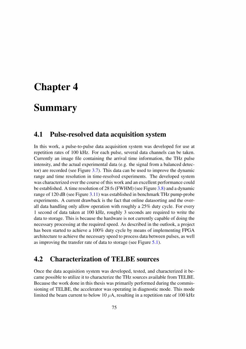
Chapter 4

Summary

4.1 Pulse-resolved data acquisition systemIn this work, a pulse-to-pulse data acquisition system was developed for use atrepetition rates of 100 kHz. For each pulse, several data channels can be taken.Currently an image file containing the arrival time information, the THz pulseintensity, and the actual experimental data (e.g. the signal from a balanced detec-tor) are recorded (see Figure 3.7). This data can be used to improve the dynamicrange and time resolution in time-resolved experiments. The developed systemwas characterized over the course of this work and an excellent performance couldbe established. A time resolution of 28 fs (FWHM) (see Figure 3.8) and a dynamicrange of 120 dB (see Figure 3.11) was established in benchmark THz pump-probeexperiments. A current drawback is the fact that online datasorting and the over-all data handling only allow operation with roughly a 25% duty cycle. For every1 second of data taken at 100 kHz, roughly 3 seconds are required to write thedata to storage. This is because the hardware is not currently capable of doing thenecessary processing at the required speed. As described in the outlook, a projecthas been started to achieve a 100% duty cycle by means of implementing FPGAarchitecture to achieve the necessary speed to process data between pulses, as wellas improving the transfer rate of data to storage (see Figure 5.1).

4.2 Characterization of TELBE sourcesOnce the data acquisition system was developed, tested, and characterized it be-came possible to utilize it to characterize the THz sources available from TELBE.Because the work done in this thesis was primarily performed during the commis-sioning of TELBE, the accelerator was operating in diagnostic mode. This modelimited the beam current to below 10 µA, resulting in a repetition rate of 100 kHz

75

76 CHAPTER 4. SUMMARY

with the desired bunch charge range of up to 100 pC. The multi-cycle superradi-ant undulator source has tunable central wavelength which can be varied between0.1 and 3 THz (see Figures 3.16 and 3.17), with a bandwidth of 20%. The pulseenergy varies based on the central frequency, with a peak of 1.3 µJ at 1 THz (seeFigure 3.17 b). The drop in intensity towards higher THz frequencies is due tolosses in the electron bunch formfactor (see Figure 2.6). The beam profile of theundulator was the expected bell shape.

The single-cycle superradiant THz source is a coherent diffraction radiation(CDR) source. This is a broadband source (0.1-2.5 THz) with a peak intensityat around 0.5 THz (with some dependence on the accelerator settings). The peakis caused by an intensity falloff towards lower frequencies caused by diffractionlosses in the transport beampipe, and a falloff towards higher frequencies causedby a combination of the electron bunch formfactor and the 4 mm central aperture(see Figure 3.23). The maximum CDR pulse energy received in the TELBE lab-oratory is in the 100 nJ range. The expected beam profile consists of two lobes,and this was observed (see Figure 3.19).

Calculations were performed to model the expected THz parameters of thesuperradiant sources at TELBE, such as spectral content, beam profile, and inten-sity. After taking the diffraction losses and polarization effects from the Brewsterangle windows into account, these calculations fit well with observations. Notethat the actual beam dynamics in the ELBE accelerator still have not been fullyestablished. Work on this is ongoing and is being undertaken by the beam dynam-ics experts, and has also been the focus of another PhD project[73]. In this thesis,the spontaneous source emissions characteristics have been established as well asscenarios for the required bunch length for reaching the THz design parameters.Assuming a Gaussian bunch form, a bunch length of 30 fs (FWHM) is required toachieve the initially prospected maximum intensity at 3 THz [74].

The development of the pulse-to-pulse data acquisition system also created away to measure pulse-to-pulse instabilities in the accelerator. By taking a mea-surement of the arrivaltime and intensity of every pulse, the arrivaltime jitter andintensity instabilities were systematically characterized. The intensity instabilitieswere surprising, with the undulator being much more stable than the CDR source(13% intensity fluctuation for the undulator, versus 21% for the CDR source, asshown in Figure 3.25). This rather significant difference has been attributed tobeam position changes within the accelerator that affect the CDR source morethan the undulator source. Arrivaltime jitter was also characterized to the high-est frequency possible, up to 50 kHz. It was only directly determined for theCDR source, with the understanding that the undulator was intrinsically synchro-nized due to the sharing of electron bunches. This intrinsic synchronization wasmeasured to be 28 fs (FWHM) (see Figure 3.8). The typical arrivaltime jitter ofthe THz sources, then, was shown to be 1.38 ps (FWHM) over the course of 1


second (see Figure 3.5 a). On longer timescales the arrivaltime will drift overlarger time ranges (Figure 5.1 in the outlook). One important finding from thesemeasurements is that the majority of the timing instabilities originate from insta-bilities with frequencies below 300 Hz. Overall, 75% of the contribution to thejitter (roughly 1 ps (FWHM)) stem from this range (see Figure 3.5 b). It wasalso shown that there is little correlation between the BAM and the arrivaltimemonitor in measured jitter frequency components [75], leading to the conclusionthat many of the BAM frequencies arise from instabilities within its own fs lasersystem, rather than originating from the accelerator. The THz-based arrivaltimemonitor developed within this thesis also suffers from this, but there are some fre-quencies that have been clearly shown to originate in the accelerator because theyalso show up in the intensity instabilities (see Table 3.1). Furthermore, there aretwo high frequency components that appear in both the BAM and THz pulse ar-rivaltime monitor at 12.7 and 22. 9 kHz. Complimentary measurements indicatethat they may originate from instabilities in the thermionic injector [21].

4.3 THz pump-fs laser probe experimentsThe TELBE facility, in combination with the pulse-resolved data acquisition sys-tem, has been successfully employed in two different benchmark THz pump-Faraday rotation probe and THz pump-THz emission probe experiments. Further-more, THz time domain spectroscopy (TDS) of the THz pulses from TELBE hasbeen performed. The latter THz spectroscopy technique was shown to exhibit anexcellent dynamic range of 106, which has not previously been seen at accelerator-based THz sources. However, the most obvious application of a high-field sourcesuch as TELBE is not linear spectroscopy, but instead the interrogation of dynam-ics driven by high-field THz pulses. Due to the currently limited frequency rangebetween 0.1 and 1 THz the scientifically most interesting processes to this end arecoherently driven spin excitations. In the first benchmark experiments, the THzdriven spin excitation in NiO [6] and in a Mn3Ga nanofilm [71] were probed bytransient Faraday rotation. The resulting dynamic range allows the extension ofthis technique to nanofilms for the first time. The second benchmark experimentinvestigated the achievable data quality in a more recently developed techniquewhich is based on the detection of the weak THz emission from the coherentlydriven spin excitation. The benchmark experiment, performed on YFeO3, showedthat an exceptional data quality can be achieved (dynamic range of 55 dB, see Fig-ure 3.30). Both experimental classes have since become the focus of the majorityof the experimental proposals for user experiments at the TELBE facility.

78 CHAPTER 4. SUMMARY

Chapter 5

Outlook

5.1 Improvement of THz pulse parametersAlthough the actual beam dynamics, bunch compression strategies, and the de-velopment of the SRF injector were not part of this thesis, but were the respon-sibility of the respective experts at HZDR, some outlook should still be givenhere. The current pulse properties of the THz sources have not yet met the designgoals put forth before the construction of TELBE (see Figure 2.1). There are sev-eral improvements planned to bring the pulse up to specifications. Currently, theELBE accelerator produces bunches with a minimum bunch length of around 1ps (FWHM). This yields maximum pulse energies of 1 µJ only up to frequencies1 THz. Assuming a purely Gaussian bunchform, to obtain the originally intendedoptimal pulse energy also up to 3 THz [74], a bunch length of less than 30 fs(FWHM) is required (see Figure 2.6 b). One result of this work is that new beamdynamics simulations are being performed by experts at HZDR to reestablish thefeasibility of their earlier handwaving prediction. Another problem is the still notfully operational SRF injector [76] which so far inhibits the high charge regime,and the prospected increase of the optimal pulse energy up to the 100 µJ regimecould not yet be shown. A first beamtime utilizing the SRF injector was performedrecently, however only at low charge and so far only moderate bunch compressionwas achieved. The hope is to operate TELBE with the high bunch charge mode ofoperation during 2017.

5.2 Arrivaltime sorting at sub-1 fs resolutionThe current arrivaltime monitor that was developed in this thesis as part of thepulse-to-pulse data acquisition system has an optimal timing resolution of 12 fs(FWHM), as determined by the physical properties of its the design. In the fol-

79

80 CHAPTER 5. OUTLOOK

lowing it shall be discussed if and how a sub-fs time resolution can be achieved.At the moment the time resolution is limited by three main contributions: the 8 ps(FWHM) wide time window, the 1.59 nm/mm linear dispersion of the spectrome-ter, and the 10 µm pixel size of the camera [7].

Figure 5.1: Illustration of the typical drift of the THz pulse arrivaltime over a 90 minuteinterval. The instability of the arrivaltime on such timescales, which correspond to atypical time for 1 minute in a THz pump-probe experiment is here 3.44 ps (FWHM). Notethat this value is FWHM, hence approximately 0.5% (around 27000) of the pulses willarrive outside of this time window. Sometimes also large drifts beyond 5 ps (FWHM)have been seen, hence a time window of ~8 ps (FWHM) is used in the arrivaltime monitorto make sure the arrivaltime of most pulses if captured. The black line is the averagearrivaltime over 1 minute, and the red area denotes the total arrivaltime jitter during thatminute.

The 8 ps (FWHM) wide time window is a limit on the arrivaltime resolution ofthe monitor because it means the spectral decoding probe pulse must be stretchedto this length to ensure that the THz pulses are always in this time window, despitethe considerable few ps (FWHM) drift and jitter observed on longer time scales(see Figure 5.1). By stabilizing the timing jitter and drift to below 1 ps (FWHM),it would be possible to reduce the size of the time window. This would in turnincrease the timing resolution of the monitor as a whole by a factor of 8, resultingin an absolute precision of 1.5 fs. Stabilization of SRF accelerators by active

5.3. ONLINE DATA-SORTING AT FULL DUTY CYCLE 81

feedback has recently been shown down to even sub-100 fs (FWHM) [13], soachieving 1 ps (FWHM) stability at ELBE is feasible.

The linear dispersion of the spectrometer affects how large a slice of timeeach pixel of the readout camera sees. This means that if one were to replace thecurrently used Princeton Instruments SP2500 spectrometer with a Princeton In-struments SP7500 [77], which has a linear dispersion of 1.03 nm/mm, you woulddecrease the size of the time window that one pixel occupies. This has the effectof stretching the current time window over more pixels. In the current setup, thatwould change the time per pixel from 12 fs to 8.3 fs. Combined with the ear-lier discussed reduction of the time window, this would result in an absolute timeresolution of 1.0 fs.

The pixel size of the camera limits the resolution much the same way the lineardispersion does. It creates a limit on how small a time slice each pixel can see.In the current setup the camera has a 10 µm pixel width [78]. There are currentlycommercial cameras available with up to 100 kHz repetition rate and a pixel sizeof 7 µm. Utilizing this type of camera would change the resolution from 12 fs to8.4 fs. Combining this improvement with the others mention above would resultin an absolute time resolution of 0.72 fs.

Improving the time resolution of the arrivaltime monitor is only one part ofthe necessary steps to achieve an overall resolution below 1 fs for the final data.The timing jitter between the CDR and undulator, for example, is in the rangeof 10 fs. In order to eliminate this it would be necessary to use the THz sourceacting as the experimental pump in the arrivaltime monitor itself. There are diffi-culties associated with this when the undulator is the source because of the longpulse length and multi-cycle nature, but solutions have been discussed and couldbe put into action in the medium term. At the few-fs timescale, smaller effectslike acoustic vibrations in mirrors and thermal expansion effects on the laser pathlength become significant, so they also must be addressed e.g. by implementingactive feedback in the laser path. Once that is achieved, however, sub-1 fs timingis clearly feasible at TELBE.

5.3 Online data-sorting at full duty cycleThere are challenges yet to be addressed regarding the arrivaltime system. Thecurrently implemented prototype system has a duty cycle of about 25%. Thismeans that if TELBE is operating at 101 kHz quasi-cw, the system can take dataon every pulse for 1-2 seconds before it must stop to write the data to storage.The goal is to further develop the system to make it capable of taking data whilewriting to storage at the same time, allowing a 100% duty cycle at 101 kHz. Thiswill of course also increase the rate that data is generated, so another challenge


that must be addressed is increasing the availability of storage and the speed thatdata is transferred to this storage. Table 5.1 shows a table of data bandwidthsrequired for various configurations of the arrivaltime monitor. Finally, after thedata is taken it must be processed into a time-resolved image of the experiment.This can take several hours using current methods and depending on the size of thedata set that was recorded. The next development at TELBE will be to increase theduty cycle of the acquisition to 100% and implementing some online processing,which requires several developments in both hardware and software.

ADC Storage neededRepetition Camera 14 bits Data rate for 30 shiftsrate 8 channels of 12 hours each101 kHz Commercial 10 MS/s 505 MB/s 654 TB101 kHz* Commercial 10 MS/s 143 MB/s 185 TB4.5 MHz KALYPSO 5 GS/s 10.3 GB/s 13.3 PB4.5 MHz* KALYPSO 5 GS/s 6.3 GB/s 8.2 PB13 MHz TBD 15 GS/s 29.8 GB/s 38.6 PB13 MHz* TBD 15 GS/s 18.2 GB/s 23.6 PBDALI 202510x100 kHz Commercial? 10 MS/s 14 bits 5 GB/s 6.54 PB10x100 kHz Commercial? 100 MS/s 16 bits 19.7 GB/s 25.6 PB

Table 5.1: Table of current and future data usage for TELBE data acquisitionsystem. *Preprocessed, which means calculating the arrivaltime of the pulse on-line and only saving that data instead of the entire image of the pulse used bythe arrivaltime monitor. Commercial camera currently in use is a Basler SprintSPL4096 line scan camera, capable of repetition rates up to 140 kHz when using2048 pixels. Data rate is the number required to calculate the required bandwidthof the network connection as well as the write speed of the storage system in or-der to take data continuously. KALYPSO refers to a fast line array currently underdevelopment [79].

5.3. ONLINE DATA-SORTING AT FULL DUTY CYCLE 83

5.3.1 HardwareOn the hardware side the current camera in use will still be adequate, but thecomputer hardware is not. A new system must be built that is capable of pullingthe arrivaltime monitor data from the camera, processing it to get an arrival time(this process currently happens offline), and then saving this data to long termstorage in between pulses. At the same time, data from the experiment must alsobe pulled from the analog-to-digital converter (ADC) and saved concurrent withthe arrivaltime data in such a way as to make sure these two data sets are associatedcorrectly with each other. Analysis of the data taken from the ADC is still plannedon being processed afterward, so that several methods can be attempted to makesure the best quality signal is extracted from the raw data. The hardware needed torecord, process, and export these two data sets in less than 10 µs (which is the timebetween pulses) means going to a system in which each data point is addressed asit comes in, instead of simply being recorded. A switch to an architecture based ona field-programmable gate array (FPGA) is planned, as this type of system shouldbe fast enough to perform these fairly basic calculations and then output the datain the time required.

5.3.2 SoftwareMoving to a new architecture requires rewriting the whole data acquisition sys-tem, although the planned changes in performance would require this even if thehardware were to remain the same. It is changing from a burst-acquire, post pro-cessing system to a real-time acquisition and processing system. Some of thework currently done offline, in which the raw data is processed to extract the ar-rival time and experimental signal, is being done instead at the time of acquisition,before the data is saved. This greatly reduces the needed network bandwidth formoving the data to storage, but also reduces the tremendous amount of storageneeded for even a few hours of measurements. Table 5.1 gives a table of the band-width required to save the data taken in various combinations of hardware whilemaintaining a duty cycle of 100%, as well as the permanent storage needed tostore 30 shifts worth of data (15 days of continuous acquisition).

Appendix A

Software

A.1 Data acquisition software

The data acquisition software was written in LabVIEW to control hardware pri-marily manufactured by National Instruments, but is flexible enough to be usedwith other hardware as well. The biggest challenge to taking data from the fastsources in use a TELBE is synchronization. Getting every piece of data correctlycorrelated is still a challenge and will be the target of some additional future de-velopment. The interface screen was designed to be relatively simple to operatewhile still providing a large variety of monitoring options to allow a user to keeptrack of the conditions of the experiment. For instance, the default view when notactively taking data shows an image of the CDR pulse as seen by the arrivaltimemonitor. A user must make certain that the timing pulse doesn’t drift out of thetime window, or timing information will be lost. Figure A.1 gives an example ofthat a user would see if they chose the option to view an online sorted step fromthe experiment. This can be used as a quick diagnostic to determine if there is areadable signal at a given time.

When the acquisition is started the software first resets the ADC, then routesthe timing signal from the timing input connection on the ADC through an internalsignal route to the image capture card. Next, a veto signal is sent to the externalpulse generator to pause the pulse output which is used as a trigger signal. Thenthe software allocates memory to store the images of the CDR pulses. There iscurrently enough memory in the system to store 2 seconds of arrivaltime data and2 seconds of data from the ADC. Next, the image capture card is initialized andthe image capture is begun. It is important to remember that at this point thetrigger signal is paused. Once everything is running the veto signal going to thepulse generator is removed, and ideally the ADC and image capture card bothreceive the next trigger pulse at the same time. In practice the image capture card

85

86 APPENDIX A. SOFTWARE

sometimes skips one trigger pulse, which requires correction later. Now the dataacquisition has started and continues for 2 seconds. The image array fills withline arrays of pixel values, and a separate array fills with data from the ADC atthe same time. When acquisition is complete the data is then moved to disk forstorage A.2. Figure A.3 gives an example of the data taken by the image capturecard. Each horizontal line is one CDR pulse. Figure A.4 shows 1 ms of the rawADC data, before any processing is performed. Figure A.5 gives an example ofthree single experimental data points. Each of these plots represents one ADCdata point, to be associated with one CDR image as represented by a single linein the arrivaltime image. This also illustrates the double-frequency probe pulsestrategy, with the first pulse shown being the signal pulse, and the second pulseshown being the background pulse to be subtracted from the signal.

A.1. DATA ACQUISITION SOFTWARE 87

Figure A.1: Image showing one of the interface screens of the data acquisition software.This particular tab contains an online representation of the sorted data that is being cur-rently acquired. Because this step requires a significant delay to process it is normallydisabled.


Figure A.2: Chart demonstrating the basics of the data acquisition system used to gatherthe data for our experiments. Initializing the hardware and synchronizing the data collec-tion were the main tasks, and writing the data to disk in a usable format was the final step.

Figure A.3: Image showing an example of the raw arrivaltime data. The data is recordedas an uncompressed TIFF image.

A.1. DATA ACQUISITION SOFTWARE 89

Figure A.4: Image showing an example of the raw balanced detector data. The data isrecorded as a 16 bit binary array.

Figure A.5: Example of a balanced detector output with a negative signal (left), positivesignal (center), and a zero signal (right). Using a sum or mean of the data points, alongwith subtracting the background signal (the pulse on the right side of each graph) allowsthe zero-signal balanced detector output to give a result of zero.


A.2 Data sorting programThe first step is to take the raw line image and convert it into a time value. This isdone by first converting each line in the image to an array of integer values, thenfiltering each array to remove high-frequency noise which can interfere with peakfinding. Then, a peak finding algorithm finds the pixel where the peak occurs.Using a previously measured calibration value, each pixel is assigned a time (forinstance, if each pixel represents a 10 fs slice of time, so the fourth pixel wouldcorrespond to an arrival time of 40 fs) and this is the arrival time of this particularpulse.

Next, the pump-probe experiment output is processed. This data consists of anarray of single-precision points taken at a rate of 10 MHz, so each point representsthe voltage reading from the detector at 100 ns intervals. The first step is to cal-culate a signal strength based on this array of data points. The described systemuses a sum of the points, but could also use a mean or some other measure, to ob-tain a single numeric value to represent signal strength. Simply using the highestdata point value introduces high-frequency noise into the signal, as well as neverreturning a zero value due to imperfect balancing in the balanced detector, so thisis generally to be avoided.

Once both an arrivaltime value and a signal value have been calculated fromthe raw data, they are matched up so that the arrivaltime measured comes from thesame electron bunch that generated the pump pulse in the pump-probe experiment.The width of the signal window is defined by the THz-laser jitter. In the describedsetup it was limited to a ±4 ps window, with most points falling toward the centerof that range. A number of measurements can be taken sequentially, each timeslightly moving the linear delay stage that is part of the probe laser beamline.The sequential measurements can be made to overlap by using small movements,increasing statistics for a better signal to noise ratio, as well as allowing processeshundreds of ps long to be measured with excellent temporal resolution. In thiscase the software will add a delay to all the points of each step which correspondsto the delay introduced by the movement of the delay stage.

A.2. DATA SORTING PROGRAM 91

Figure A.6: Image of the interface of the data sorting program. It shows various diag-nostics that display how well the program is working and allow the user to control inputvariables that describe how the data was recorded in order to get the correct output.


Figure A.7: Example of the 200 kHz laser noise subtraction technique. Red shows aMOKE measurement of a 1 THz oscillation of a 50 µm NiO film, taken with the probelaser operating at the same repetition rate as the THz. Black shows the same measurement,but using a probe beam operating at double the THz repetition rate and subtracting thesecond, unmodified pulse from the first one. This reduces noise originating in the laserintensity jitter. The effect is most clearly seen as subtraction of a DC value from thesignal. There is also some small improvement in the noise visible with subtraction. Datataken with 101 kHz repetition rate, 24 MeV beam energy, and 70 pC bunch charge.

Appendix B

Additional figures

Figure B.1: Carrier envelope phase in the time domain: A pulse train of five consecutivepulses with linearly varying CEP is depicted. Depending on its value the relative delaybetween the carrier (black) and the envelope (blue dashed) is different. Taken from [80].

93

94 APPENDIX B. ADDITIONAL FIGURES

(a)

(b)

Figure B.2: Low-frequency portion of the spectrum of the intensity fluctuations of theCDR and undulator sources at TELBE. It can seen that a subset of frequencies are sharedin between the CDR and undulator sources. The frequency of 50 Hz marked with a # is180 out of phase between the two sources, and can be attributed to instabilities of thebeam position.

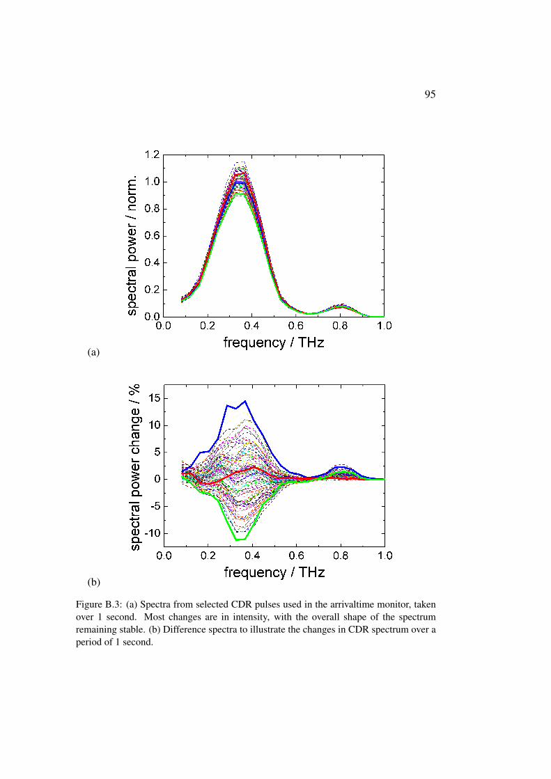
95

(a)

(b)

Figure B.3: (a) Spectra from selected CDR pulses used in the arrivaltime monitor, takenover 1 second. Most changes are in intensity, with the overall shape of the spectrumremaining stable. (b) Difference spectra to illustrate the changes in CDR spectrum over aperiod of 1 second.


Freq. (Hz) CDR Undulator CDR BAMintensity intensity Arrivaltime

260 +++950 +

7600 +8900 +++

10900 +13969 +++16300 ++16564 +17100 ++17801 +++19036 +19500 ++21633 -25400 ++26701 +++27583 +27685 +27938 +++28955 +31300 ++32900 +33800 ++34600 ++35602 +++36399 ++36838 +39000 +39435 +40670 ++41782 +++41907 +++42031 +42200 +++43200 ++43612 +43775 +44503 +++46500 +

97


46974 +++49300 +++

Table B.1: Frequency components only visible in one of the arrivaltime measure-ments.


50 +++# ++#

68 +132 +++ ++ +160 ++# +#

166 ++ ++ +193 +# +#

260 +++527 + +++3634 +7600 +8089 +8273 +8900 +++

10900 +11908 ++12732 + +(12.8kHz)13969 +++14312 +16300 ++16520 +16564 +17100 ++17801 +++18450 +19036 +19500 ++20401 + +21633 +22869 ++ ++(22.7kHz)25400 ++



26701 +++27450 +27583 +27685 +27938 +++28063 + ++(28.1kHz)28955 +28961 ++* +*

29295 +31085 +31300 ++32900 +33800 ++34600 ++35602 +++36265 +36315 +++* +*

36399 ++36365 +36734 +36838 +39000 +39435 +40670 ++41782 +++41907 +++42031 +42200 +++42993 +43200 ++43608 ++* +*

43612 +43775 +44503 +++46500 +46628 ++46974 +++48250 +

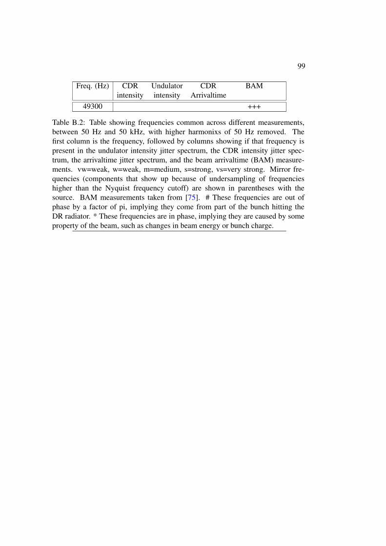
99


49300 +++

Table B.2: Table showing frequencies common across different measurements,between 50 Hz and 50 kHz, with higher harmonixs of 50 Hz removed. Thefirst column is the frequency, followed by columns showing if that frequency ispresent in the undulator intensity jitter spectrum, the CDR intensity jitter spec-trum, the arrivaltime jitter spectrum, and the beam arrivaltime (BAM) measure-ments. vw=weak, w=weak, m=medium, s=strong, vs=very strong. Mirror fre-quencies (components that show up because of undersampling of frequencieshigher than the Nyquist frequency cutoff) are shown in parentheses with thesource. BAM measurements taken from [75]. # These frequencies are out ofphase by a factor of pi, implying they come from part of the bunch hitting theDR radiator. * These frequencies are in phase, implying they are caused by someproperty of the beam, such as changes in beam energy or bunch charge.

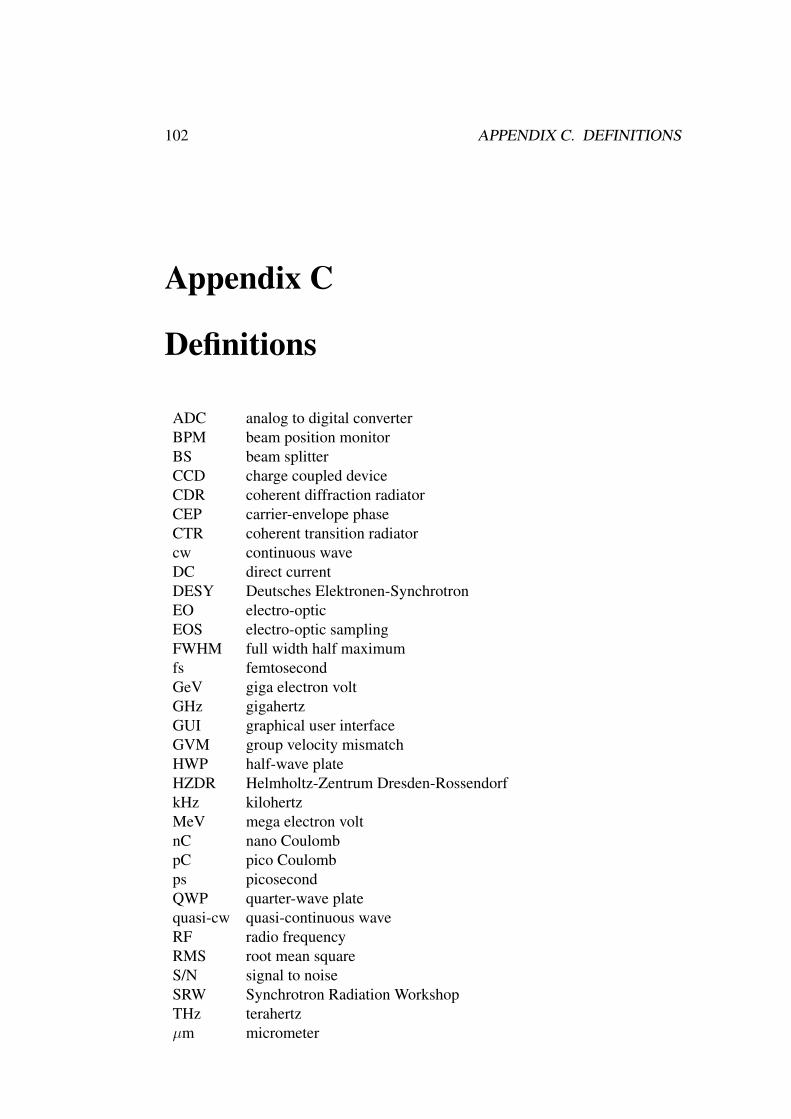
102 APPENDIX C. DEFINITIONS

Appendix C

Definitions

ADC analog to digital converterBPM beam position monitorBS beam splitterCCD charge coupled deviceCDR coherent diffraction radiatorCEP carrier-envelope phaseCTR coherent transition radiatorcw continuous waveDC direct currentDESY Deutsches Elektronen-SynchrotronEO electro-opticEOS electro-optic samplingFWHM full width half maximumfs femtosecondGeV giga electron voltGHz gigahertzGUI graphical user interfaceGVM group velocity mismatchHWP half-wave plateHZDR Helmholtz-Zentrum Dresden-RossendorfkHz kilohertzMeV mega electron voltnC nano CoulombpC pico Coulombps picosecondQWP quarter-wave platequasi-cw quasi-continuous waveRF radio frequencyRMS root mean squareS/N signal to noiseSRW Synchrotron Radiation WorkshopTHz terahertzµm micrometer

Bibliography

[1] S. S. Dhillon et al. The 2017 terahertz science and technology roadmap. J.Phys. D: Appl. Phys., 50:043001, 2017.

[2] C. A. Schmuttenmaer. Exploring dynamics in the far-infrared with terahertzspectroscopy. Chem. Rev., 104:1759, 2004.

[3] T. Kampfrath, K. Tanaka, and K. A. Nelson. Resonant and nonresonantcontrol over matter and light by intense terahertz transients. Nat. Photon., 7:680, 2013.

[4] N. Stojanovic and M. Drescher. Accelerator- and laser-based sources ofhigh-field terahertz pulses. J. Phys. B, 46:192001, 2013.

[5] Z. Wu et al. Intense terahertz pulses from slac electron beams using coherenttransition radiation. Rev. Sci. Instr., 84:022701, 2013.

[6] B. Green et al. High-field high-repetition-rate sources for the coherent THzcontrol of matter. Sci. Rep., 6:22256, 2016.

[7] S. Kovalev et al. Probing ultra-fast processes with high dynamic range at4th-generation light sources. Struct. Dyn., 4:024301, 2017.

[8] B. Aune et al. Superconducting TESLA cavities. Phys. Rev. ST AB, 3:092001, 2000.

[9] X. Ding and S. Boucher. A method for establishing Q-factors of RF cavities.Proceedings of IPAC ’10, Kyoto, Japan, page 3789, 2010.

[10] Mitsubishi Heavy Industries. Mitsubishi heavy industries’ normal conduct-ing/superconducting accelerating cavities - contributing to the developmentof highly-advanced particle accelerator systems. Mitsubishi Heavy Indus-tries Technical Review, 53:25, 2016.

[11] H. Padamsee. RF Superconductivity. Wiley-VCH, first edition, 2009.

103

104 BIBLIOGRAPHY

[12] F. Loehl et al. Electron bunch timing with femtosecond precision in a super-conducting free-electron laser. Phys. Rev. Lett, 104:144801, 2010.

[13] S. Schulz et al. Femtosecond all-optical synchronization of an X-ray free-electron laser. Nucl. Instr. Meth. Phys. Res. A, 507:354, 2003.

[14] W. Wuensch et al. A demonstration of high-gradient acceleration. Proceed-ings of the 2003 Particle Accelerator Conference, page 495, 2003.

[15] J. Teichert et al. Results of beam parameter measurement of the ELBE elec-tron accelerator after commissioning. Nucl. Instr. Meth. Phys. Res. A, 507:354, 2003.

[16] P. Michel et al. The Rossendorf IR-FEL ELBE. Proceedings of FEL 2006,page 488, 2006.

[17] R. Krause-Rehberg et al. EPOS - an intense positron beam project at theELBE radiation source in rossendorf. Appl. Surf. Sci., 252:3106, 2006.

[18] E. Altstadt et al. A photo-neutron source for time-of-flight measurements atthe radiation source elbe. Ann. Nucl. Energy, 34:36, 2007.

[19] R. Schwengner et al. The photon-scattering facility at the superconductingelectron accelerator elbe. Nucl. Instr. Meth. Phys. Res. A, 555:211, 2005.

[20] F. Gabriel et al. The Rossendorf radiation source ELBE and its FEL projects.Nucl. Instr. Meth. Phys. Res. B, 161:1143, 2000.

[21] M. Kuntzsch/HZDR. private communication, 2016.

[22] CPI. Electron sources, 2016. URL http://www.cpii.com/docs/datasheets/131/Electron%20Guns%20Data%20Sheet6.pdf.

[23] ELBE. Pulsed injector, 2016. URL https://www.hzdr.de/db/Cms?pNid=971.

[24] H. Buettig/HZDR. private communication, 2016.

[25] H. Buettig et al. RF power upgrade at the superconducting 1.3 GHz CWLINAC ELBE with solid state amplifiers. Nucl. Instr. Meth. Phys. Res. A,704:7–13, 2013.

[26] Libera. Performance, Reliability, Cost Effectiveness = Libera Spark,2016. URL http://www.i-tech.si/announcements/performance-reliability-cost-effectiveness--libera-spark.

http://www.cpii.com/docs/datasheets/131/Electron%20Guns%20Data%20Sheet6.pdf

http://www.cpii.com/docs/datasheets/131/Electron%20Guns%20Data%20Sheet6.pdf

https://www.hzdr.de/db/Cms?pNid=971

https://www.hzdr.de/db/Cms?pNid=971

http://www.i-tech.si/announcements/performance-reliability-cost-effectiveness--libera-spark

http://www.i-tech.si/announcements/performance-reliability-cost-effectiveness--libera-spark

BIBLIOGRAPHY 105

[27] S. Casalbuoni, B. Schmidt, and P. Schmüser. Far-infrared transition anddiffraction radiation. TESLA Report 2005-15, 2005.

[28] U. Lehnert/HZDR. private communication, 2016.

[29] G.L. Carr et al. High-power terahertz radiation from relativistic electrons.Nature, 420:153–156, 2002.

[30] V. Ginzburg and I. Frank. Radiation of a uniformly moving electron dueto its transition from one medium into another. Zhurnal Eksperimentalnoi ITeoreticheskoi Fiziki, 16:15, 1946.

[31] M. Castellano, A. Cianchi, G. Orlandi, and V.A. Verzilov. Effects of diffrac-tion and target finite size on coherent transition radiation spectra in bunchlength measurements. Nucl. Instr. Meth. Phys. Res. A, 435:297, 1999.

[32] V. Ginzburg. Bull. Acad. Sci. U.S.S.R. Sér. Phys., 11:165, 1947.

[33] F. R. Elder et al. Radiation from electrons in a synchrotron. Phys. Rev., 71:829, 1947.

[34] H. Motz, W. Thon, and R.N. Whitehurst. Experiments on radiation by fastelectron beams. J. Appl. Phys., 24:826, 1953.

[35] H. Wiedemann. Particle Accelerator Physics. Springer, third edition, 2007.

[36] K-J Kim. Characteristics of synchrotron radiation. AIP Conf. Proc., 184:565, 1989.

[37] E. R. Caley and J. F. C. Richards. Theophrastus: On Stones. Ohio StateUniversity Press, 1 edition, 2016.

[38] D. Brewster. Observations of the pyro-electricity of minerals. The EdinburghJournal of Science, 1:208, 1824.

[39] L. D. Landau, E. M. Lifschitz, and L. P. Pitaevski, editors. Electrodynamicsof Continuous Media. Elsevier, second edition, 2007.

[40] S. Wesch et al. A multi-channel THz and infrared spectrometer for fem-tosecond electron bunch diagnostics by single-shot spectroscopy of coherentradiation. Nucl. Instr. Meth. Phys. Res. A, 665:40, 2012.

[41] DIAS Infrared GmbH. Pyroelectric infrared detectors, 2006. URL www.dias-infrared.de/pdf/basics_eng.pdf.

www.dias-infrared.de/pdf/basics_eng.pdf

www.dias-infrared.de/pdf/basics_eng.pdf

106 BIBLIOGRAPHY

[42] T. Crowe et al. Opening the THz window with integrated diode circuits.IEEE J. Solid-State Circuits, 40-10:2104, 2005.

[43] I. Ederra et al. Design and test of a 0.5 THz dipole antenna with integratedschottky diode detector on a high dielectric constant ceramic electromag-netic bandgap substrate. IEEE Trans. THz Sci. Technol., 3-5:584, 2013.

[44] N. Neumann/TU Dresden. private communication, 2016.

[45] M. Schiselski et. al. A planar schottky diode based integrated THz detectorfor fast electron pulse diagnostics, 2016.

[46] K.-E. Peiponen, J. A. Zeitler, and M. Kuwata-Gonokami, editors. TerahertzSpectroscopy and Imaging. Springer, first edition, 2013.

[47] Q. Wu and X.-C. Zhang. Ultra fast electro-optic field sensors. Appl. Phys.Lett., 68:1604, 1996.

[48] P. Planken. Measurement and calculation of the orientation dependence ofterahertz pulse detection in ZnTe. J. Opt. Soc. Am. B, 18:313, 2001.

[49] Z. Jiang and X.-C. Zhang. Measurement of spatio-temporal terahertz fielddistribution by using chirped pulse technology. IEEE J. Quant. Electron.,36:1214, 2000.

[50] Ophir Optics. Ophir optics pyrocam 3, 2016. URLhttp://www.ophiropt.com/laser--measurement/beam-profilers/products/Beam-Profiling/Camera-Profiling-with-BeamGage/Pyrocam-IIIHR.

[51] A. Steiger et al. Traceable THz power measurement from 1 THz to 5 THz.Opt. Express, 21:14466, 2013.

[52] Ophir Optics. Laser power sensors introduction, 2016. URL http://www.ophiropt.com/laser-measurement-instruments/laser-power-energy-meters/tutorial/thermal-sensors.

[53] B. Schmidt/DESY. private communication, 2016.

[54] F. Loehl et al. High bandwidth pickup design for bunch arrival-time monitorsfor free-electron laser. Phys. Rev. Lett., 104:144801, 2010.

[55] F. Tavella, N. Stojanovic, G. Geloni, and M. Gensch. Few-femtosecondtiming at fourth-generation X-ray light sources. Nat. Photon., 5:162, 2011.

http://www.ophiropt.com/laser--measurement/beam-profilers/products/Beam-Profiling/Camera-Profiling-with-BeamGage/Pyrocam-IIIHR



http://www.ophiropt.com/laser-measurement-instruments/laser-power-energy-meters/tutorial/thermal-sensors




BIBLIOGRAPHY 107

[56] J. Shan et. al. Single-shot measurement of terahertz electromagnetic pulsesby use of electro-optic sampling. Opt. Lett., 25-6:426, 2000.

[57] Coherent. RegA Data Sheet, 2016. URL https://cohrcdn.azureedge.net/assets/pdf/RegA-Data-Sheet.pdf#page=1.

[58] Coherent. Coherent, 2016. URL https://www.coherent.com/.

[59] Coherent. Synchrolock-AP, 2016. URL https://www.coherent.com/lasers/laser/ultrafast-oscillator-accessories/synchrolock-ap.

[60] S. Kovalev/HZDR. private communication, 2016.

[61] M. J. Rosker, M. Dantus, and A. H. Zewail. Femtosecond real-time probingof reactions. I. the technique. J. Chem. Phys., 89:6113, 1988.

[62] U. Fruehling et al. Single-shot terahertz-field-driven X-ray streak camera.Nat. Photon., 3:523, 2009.

[63] W. Withayachumnankul and M. J. Naftaly. Fundamentals of measurementin terahertz time-domain spectroscopy. J. Infrared Millim. Terahertz Waves,35:610, 2014.

[64] O. Chubar, P. Elleaume, and A. Snigirev. Phase analysis and focusing ofsynchrotron radiation. Nucl. Instr. Meth. Phys. Res. A, 435:495, 1999.

[65] M. Gensch. Superradiant linac-based THz sources in 2013. Proceedings ofFEL2013, 2013.

[66] D. Suetterlin et al. An analytic formalism for the emission of coherent tran-sition radiation from an oblique finite thin metallic target screen. Nucl. Instr.Meth. Phys. Res. B, 264:361, 2007.

[67] M. Schwarz et al. Comparison of various sources of coherent THz radiationat FLUTE. Proceedings of IPAC 2012, page 568, 2012.

[68] H. Nyquist. Certain factors affecting telegraph speed. Bell System TechnicalJournal, 3:324, 1924.

[69] W. S. Fann et al. Direct measurement of nonequilibrium electron-energydistributions in subpicosecond laser-heated gold films. Phys. Rev. Lett., 68:2834, 1992.

https://cohrcdn.azureedge.net/assets/pdf/RegA-Data-Sheet.pdf#page=1



https://www.coherent.com/

https://www.coherent.com/lasers/laser/ultrafast-oscillator-accessories/synchrolock-ap



108 BIBLIOGRAPHY

[70] F. Kuschewski. Optical nanoscopy of transient states in condensed matter.Sci. Rep., 5:12582, 2015.

[71] N. Awari et al. Narrow-band tunable terahertz emission from ferrimagneticMn3-xGa thin films. Appl. Phys. Lett., 109:032403, 2016.

[72] Z. Jin et al. Single-pulse terahertz coherent control of spin resonance inthe canted antiferromagnet YFeO3, mediated by dielectric anisotropy. Phys.Rev. B, 87:094422, 2013.

[73] P. Lu. Optimization of an SRF Gun for High Bunch Charge Applications atELBE. PhD thesis, Technisch Universität Dresden, 2017.

[74] U. Lehnert/HZDR. private communication, 2011.

[75] M. Kuntzsch. Optische Synchronisation am CW-Beschleuniger ELBE. PhDthesis, Technisch Universität Dresden, 2015.

[76] P. Murcek et al. The SRF photo injector at ELBE - design and status 2013.Proceedings of SRF2013, page 148, 2013.

[77] Princeton Instruments. High-performance imaging spectrographsand scanning monochromators, 2016. URL http://www.princetoninstruments.com/products/SpectraPro.

[78] Basler. spL4096-140km, 2016. URL http://www.baslerweb.com/en/products/cameras/line-scan-cameras/sprint/spl4096-140km.

[79] L. Rota et al. KALYPSO: A linear array detector for visible to NIR radiation.Proceedings of IBIC2016, page 740, 2016.

[80] D. Jones et al. Carrier-envelope phase control of femtosecond mode-lockedlasers and direct optical frequency synthesis. Science, 288:635, 2000.

http://www.princetoninstruments.com/products/SpectraPro

http://www.princetoninstruments.com/products/SpectraPro

http://www.baslerweb.com/en/products/cameras/line-scan-cameras/sprint/spl4096-140km



Acknowledgments

This thesis encompassed a lot of life-changing events for me. It all started afteran international move to a place where I didn’t speak the language (and still onlybarely do, sorry guys). The birth of my son, Marcus, and later the birth of mydaughter Ilona. The loss of two cats, my cat Boots who had been with me for 15years, and my wife’s cat Shira, show had been with her for 12 years. I became agodfather to a wonderful little boy, Felix Steinbrück, who I will hopefully get tosee more often once this is all finished.

I would first like to thank my ever-patient wife Liz. During the course of thisthesis she would often take the kids on trips or wake up with them at night so Iwould have a chance to work. Without her support I never would have been ableto finish.

I would also like to thank my group. Dr. Sergey Kovalev with whom I workedclosely to develop the data acquisition and data analysis systems. He provided alot of expertise on electro-optic sampling and spectral decoding. We also spentmany frustrating and fruitful night shifts performing experiments, rewriting soft-ware, and aligning lasers. Dr. Jan-Christoph Deinert, who although he showedup towards the end still provided valuable advice for writing. Nilesh Awari andMin Chen, my fellow students in the group who will soon be defending their owntheses.

Coworkers at ELBE also provided help and support. Special thanks to Rein-hard Steinbrück, who provided not only advice on LabVIEW programming andhardware acquisition but also friendship. Dr. Ulf Lehnert, who provided muchvaluable information on the ELBE accelerator. Dr. Hartmut Büttig for provid-ing books, papers, and occasional custom hardware as well as being one of thefriendliest people I know. Dr. Michal Kuntzsch, whose valuable work and adviceon synchronization with the ELBE timing distribution system helped make thearrivaltime monitor possible. Petra Neumann, who put up with my constant ques-tions and inability to properly fill out all types of paperwork. Hannes Vennekatefor being helpful and friendly and always having time for a chat about America.Dr. Michael Klopf, for providing wonderful advice and a whole slew of papersand references.

109

110 ACKNOWLEDGMENTS

I’d also like to thank the FLASH crew, for hosting me during beamtimes aswell as coming to help with beamtimes here: Torsten Golz and Nikola Stojanovicespecially.

Thanks go to many other outside collaborators as well. Dr. Nicole Hillerfrom KIT for being my go-to for any questions regarding thesis writing and near-field electro-optic sampling. Dr. Markus Schwarz, also from KIT, for workingwith me on simulations and analytical calculations. Dr. Gianluca Geloni fromEuropean XFEL and Dr. Vivek Asgekar, visiting us from India, for all their helpwith undulator simulations and explanations about the SRW software package.Special thanks also go to Dr. Alan Fisher of SLAC, for his help with CDR andCTR simulations as well as inviting me on a fascinating tour of the facilities atSLAC.

superradiant terahertz sources and their applications in

Documents