supervised tensor learning

Knowl Inf Syst (2006)DOI 10.1007/s10115-006-0050-6

Knowledge andInformation Systems

REGULAR PAPER

Dacheng Tao · Xuelong Li · Xindong Wu ·Weiming Hu · Stephen J. Maybank

Supervised tensor learning

Received: 30 November 2005 / Revised: 10 July 2006 / Accepted: 18 August 2006C© Springer-Verlag London Limited 2006

Abstract Tensor representation is helpful to reduce the small sample size prob-lem in discriminative subspace selection. As pointed by this paper, this is mainlybecause the structure information of objects in computer vision research is a rea-sonable constraint to reduce the number of unknown parameters used to representa learning model. Therefore, we apply this information to the vector-based learn-ing and generalize the vector-based learning to the tensor-based learning as thesupervised tensor learning (STL) framework, which accepts tensors as input. Toobtain the solution of STL, the alternating projection optimization procedure isdeveloped. The STL framework is a combination of the convex optimization andthe operations in multilinear algebra. The tensor representation helps reduce theoverfitting problem in vector-based learning. Based on STL and its alternating pro-jection optimization procedure, we generalize support vector machines, minimaxprobability machine, Fisher discriminant analysis, and distance metric learning,to support tensor machines, tensor minimax probability machine, tensor Fisherdiscriminant analysis, and the multiple distance metrics learning, respectively. Wealso study the iterative procedure for feature extraction within STL. To examinethe effectiveness of STL, we implement the tensor minimax probability machinefor image classification. By comparing with minimax probability machine, thetensor version reduces the overfitting problem.

D. Tao (B) · X. Li · S. J. MaybankSchool of Computer Science and Information Systems, Birkbeck, University of London,London, UKE-mail: [email protected]

X. WuDepartment of Computer Science, University of Vermont, Burlington, VT, USA

W. HuNational Laboratory of Pattern Recognition, Institute of Automation, Chinese Academy ofSciences, Beijing, P.R. China

D. Tao et al.

Keywords Convex optimization · Supervised learning · Tensor · Alternatingprojection

1 Introduction

In computer vision research, many objects are naturally represented by multidi-mensional arrays, i.e., tensors [17], such as the gray face image shown in Fig. 1 inface recognition [7, 48], the color image shown in Fig. 2 in scene image classifica-tion [40, 41], and the video shot shown in Fig. 3 in motion categorization [11, 26].However, in current research, the original tensors (images and videos) are alwaysscanned into vectors, thus discarding a great deal of useful structural information[36, 38, 52, 53], which is helpful to reduce the small sample-size (SSS) problemin subspace selection methods, e.g., linear discriminant analysis (LDA).

To utilize this structure information, many dimension reduction algorithms[17, 29, 38, 46, 51, 52] based on the multilinear subspace method (MLSM)have been developed for data representation [17, 29, 46, 51], pattern classifica-tion [38, 36, 52], and network abnormal detection [33]. This structure informa-tion of objects in computer vision research is a reasonable constraint to reducethe number of unknown parameters used to represent a learning model. MLSMfinds a sequence of linear transformation matrices Ui ∈ RLi ×L ′

i (L ′i < Li ,

1 ≤ i ≤ M) to transform a big-size tensor X ∈ RL1×L2×···×L M to a small-size

SecondOrder Tensor

Width

Hei

ght

Face Image

Fig. 1 A gray face image is a second-order tensor, which is also a matrix. Two indicesare required for pixel locations. The face image comes from http://www.merl.com/projects/images/face-rec.gif

Third OrderTensor

Width

Hei

ght

Color

Color Image

Fig. 2 A color image is a third-order tensor, which is also a data cuboid, because three indicesare required to locate elements. Two indices are used for pixel locations and one index is usedto local the color information (e.g., R, G, and B)


Fourth Order Tensor

Width

Hei

ght

Color Video Shot

Tim

e

Color

Time

Fig. 3 A color video shot is a fourth-order tensor. Four indices are used to locate elements.Two indices are used for pixel locations; one index is used to local the color information; andthe other index is used to represent the time varying. The video shot comes from http://www-nlpir.nist.gov/projects/trecvid/

tensor Y ∈ RL ′1×L ′

2×···×L ′M , i.e., Y = X×1 U T

1 ×2 U T2 ×· · ·×M U T

M . For example,if we have a big second order tensor (i.e., a big matrix) X ∈ RL1×L2 , in MLSMwe need to find two linear transformation matrices U1 ∈ RL1×L ′

1 (L ′1 < L1 ) and

U2 ∈ RL2×L ′2 (L ′

2 < L2) to transform the big matrix to a small matrix accordingto Y = X ×1 U T

1 ×2 U T2 , i.e., Y = U T

1 XU2. After the transformation, the original

datum dimension is reduced from L1 × L2 to L ′1 × L ′

2 , i.e., Y ∈ RL ′1×L ′

2 .The structure information can also be utilized to vector-based learning to re-

duce the overfitting problem when measurements are limited. In vector-basedlearning [6, 9], a projection vector �w ∈ RL and a bias b ∈ R are learnt to de-termine the class label of a measurement �x ∈ RL according to a linear decisionfunction y (�x) = sign[ �wT �x + b]. The �w and b are obtained based on a learningmodel, e.g., minimax probability machine (MPM) [16, 31], based on N trainingmeasurements associated with labels {�xi ∈ RL , yi }, where yi is the class label,yi ∈ {+1, −1}, and 1 ≤ i ≤ N .

The supervised tensor learning (STL) [36] is developed to extend the vector-based learning algorithms to accept tensors as input. That is, we learn a seriesof projection vectors �wk |M

k=1 ∈ RLk and a bias b ∈ R to determine the classlabel {+1,−1} of a measurement X ∈ RL1×L2×···×L M according to a multilin-ear decision function y (X) = sign[X∏M

k=1 ×k �wk + b]. The projection vectors�wk |M

k=1 and the bias b are obtained from a learning model, e.g., tensor minimaxprobability machine (TMPM), based on N training measurements associated withlabels {Xi ∈ RL1×L2×···×L M , yi }, where yi is the class label, yi ∈ {+1,−1}, and

D. Tao et al.

1 ≤ i ≤ N . To obtain the solution of the algorithms under STL framework,we develop the alternating projection optimization procedure. Based on STL andits alternating projection optimization procedure, we illustrate several examples,which are support tensor machines (STMs), tensor minimax probability machine(TMPM), tensor Fisher discriminant analysis (TFDA), multiple distance metricslearning (MDML).

This paper is organized as follows. Section 2 introduces tensor algebra.Section 3 gives the relatiobship between LSM and MLSM. In Section 4, the con-vex optimization is briefly reviewed and a framework-level formula of the con-vex optimization-based learning is introduced. In Section 5, we develop the su-pervised tensor learning (STL) framewok, which is an extension of the convexoptimization-based learning. The alternating projection method is also developedto obtain the solution to an STL-based learning algorithm. In Section 6, we de-velop a number of tensor extensions of many popular learning machines, such asthe support vector machines (SVM) [5, 27, 28, 34, 35, 45], the minimax prob-ability machine (MPM) [16, 31], the Fisher discriminant analysis (FDA) [6, 8,14], and the distance metric learning (DML) [49]. In Section 7, an iterative fea-ture extraction model is given as an extension of the STL framework. Experi-ments in Section 8 based on TMPM show that tensor representation is helpfulto reduce the overfitting problem in vector-based learning. Section 9 providesconclusions.

2 Tensor algebra

This section contains the fundamental materials on tensor algebra [17], whichare relevant to this paper. Tensors are arrays of numbers that transform in cer-tain ways under different coordinate transformations. The order of a tensor X ∈RL1×L2×···×L M , represented by a multidimensional array of real numbers, is M .An element of X is denoted as Xl1,l2,...,lM , where 1 ≤ li ≤ Li and 1 ≤ i ≤ M .The i th dimension (or mode) of X is of size Li . A scalar is a zeroth-order tensor;a vector is a first-order tensor; and a matrix is a second-order tensor. A third-ordertensor as an example is shown in Fig. 4. In the tensor terminology, we have thefollowing definitions.

1 2 3L L LR × ×∈X1L

2L3L

Fig. 4 A third-order tensor X ∈ RL1×L2×L3


Definition 2.1 (Tensor Product or Outer Product) The tensor product X ⊗ Y of atensor X ∈ RL1×L2×···×L M and another tensor Y ∈ RL ′

1×L ′2×···×L ′

M ′ is defined by

(X ⊗ Y)l1×l2×···×lM×l ′1×l ′2×···×l ′M ′ = Xl1×l2×···×lM Yl ′1×l ′2×···×l ′

M ′ (1)

for all index values.For example, the tensor product of two vectors �x1 ∈ RL1 and �x2 ∈ RL2 is a

matrix X ∈ RL1×L2 , i.e., X = �x1 ⊗ �x2 = �x1 �xT2 .

Definition 2.2 (Mode-d Matricizing or Matrix Unfolding) The mode-d matriciz-ing or matrix unfolding of an M th-order tensor X ∈ RL1×L2×···×L M is the setof vectors in RLd obtained by keeping the index id fixed and varying the otherindices. Therefore, the mode-d matricizing or matrix unfolding of an Mth-ordertensor is a matrix X(d) ∈ RLd×Ld , where Ld = (

∏i �=d Li ). We denote the mode-d

matricizing of X as matd(X) or briefly X(d).

Definition 2.3 (Tensor Contraction) The contraction of a tensor is obtained byequating two indices and summing over all values of the repeated indices. Con-traction reduces the tensor order by 2. A notation is the Einstein’s summation con-vention.1 For example, the tensor product of two vectors �x, �y ∈ RN is Z = �x ⊗ �y;and the contraction of Z is Zii = �x · �y = �xT �y, where the repeated indices implysummation. The value of Zii is the inner product of �x and �y. In general, for tensorsX ∈ RL1×···×L M×L ′

1×···×L ′M ′ and Y ∈ RL1×···×L M×L ′′

1×···×L ′′M ′′ , the contraction on

the tensor product X ⊗ Y is

[[X ⊗ Y; (1 : M) (1 : M)]]

=L1∑

l1=1

· · ·L M∑

lM=1

(X)l1×···×lM×l ′1×···×l ′M ′ (Y)l1×···×lM×l ′′1 ×···×l ′′

M ′′ . (2)

In this paper, when the convention is conducted on all indices but the index i onthe tensor product of X and Y in RL1×L2×···×L M , we denote this procedure as

[[X ⊗ Y; (i) (i)]] = [[X ⊗ Y; (1 : i − 1, i + 1 : M) (1 : i − 1, i + 1 : M)]]

=L1∑

l1=1

· · ·Li−1∑

li−1=1

Li+1∑

li+1=1

· · ·L M∑

lM=1

×(X)l1×···×li−1×li ×li+1×···×lM(Y)l1×···×li−1×li ×li+1×···×lM

= mati (X) matTi (Y) = X(i)YT(i), (3)

and [[X ⊗ Y; (i) (i)]] ∈ RLi ×Li .

1 When any two subscripts in a tensor expression are given the same symbol, it is implied thatthe convention is formed.–A. Einstein, Die Grundlage der Allgemeinen Relativitatstheorie, Ann.Phys., 49:769, 1916.

D. Tao et al.

Definition 2.4 (Mode-d product) The mode-d product X ×d U of a tensor X ∈RL1×L2×···×L M and a matrix U ∈ RL ′

d×Ld is an L1×L2×· · ·×Ld−1×L ′d×Ld+1×

· · · × L M tensor defined by

(X×dU )l1×l2×···×ld−1×l ′d×ld+1×···×lM=∑

l ′d

(Xl1×l2×···×ld−1×ld×ld+1×···×lM Ul ′d×ld

),

(4)for all index values. The mode-d product is a type of contraction.

Based on the definition of Mode-d product, we have

(X ×d U ) ×t V = (X ×t V ) ×d U, (5)

where X ∈ RL1×L2×···×L M , U ∈ RL ′d×Ld , and V ∈ RL ′

t ×Lt . Therefore,(X ×d U ) ×t V can be simplified as X ×d U ×t V .

Furthermore,(X ×d U ) ×t V = X ×d (V U ) , (6)

where X ∈ RL1×L2×···×L M , U ∈ RL ′d×Ld , V ∈ RL ′′

d×L ′d , and V U is the standard

matrix product between V and U.To simplify the notation in this paper, we denote

X ×1 U1 ×2 U2 × · · · ×M UM�= X

M∏

k=1

×k Uk, (7)

and

X ×1 U1×· · ·×i−1 Ui−1 ×i+1 Ui+1 × · · · ×M UM = XM∏

d=1;d �=i

×d Ud�= X×iUi .

(8)

Definition 2.5 (Frobenius Norm) The Frobenius norm of a tensor X ∈RL1×L2×···×L M is given by

‖X‖Fro = √[[X ⊗ X; (1 : M) (1 : M)]] =

√√√√√

L1∑

l1=1

· · ·L M∑

lM=1

X2l1×···×lM

. (9)

The Frobenius norm of a tensor X measures the size of the tensor and itssquare is the energy of the tensor.

Definition 2.6 (Rank-1 tensor) An M th-order tensor X has rank one if it is thetensor product of M vectors �ui ∈ RLi , where 1 ≤ i ≤ M

X = �u1 ⊗ �u2 ⊗ · · · ⊗ �uM =M∏

k=1

⊗�uk . (10)

The rank of an arbitrary M th-order tensorX, denoted by R = rank (X) , is theminimum number of rank-1 tensors that yield X in a linear combination.


3 The relationship between LSM and MLSM

Suppose: 1) we have a dimension reduction algorithm A1 , which finds a se-quence of linear transformation matrices Ui ∈ RLi ×L ′

i (L ′i < Li , 1 ≤ i ≤ M)

to transform a big-size tensor X ∈ RL1×L2×···×L M to a small-size tensor Y1 ∈RL ′

1×L ′2×···×L ′

M , i.e., Y1 = X ×1 U T1 ×2 U T

2 × · · · ×M U TM ; and 2) we have an-

other dimension reduction algorithm A2 , which finds a linear transformation ma-trix U ∈ RL×L ′

(L = L1×L2×· · ·×L M and L ′ = L ′1×L ′

2×· · ·×L ′M ; L ′

i < Li )to transform a high-dimensional vector �x = vect (X) to a low-dimensional vec-tor �y2 = vect (Y2), i.e., �y2 = U T �x , where vect (·) is the vectorization operator;�x ∈ RL and �y2 ∈ RL ′

. According to [55], we know

�y1 = vect (Y1)

= vect(

X ×1 U T1 ×2 U T

2 × · · · ×M U TM

)

= (U1 ⊗ U2 ⊗ · · · ⊗ UM )T vect (X) . (11)

Therefore, if U = U1 ⊗ U2 ⊗ · · · ⊗ UM , �y2 = �y1. That is, the algorithm A1

equals algorithm A2, if the linear transformation matrix U ∈ RL×L ′in A2 equals

to U1 ⊗ U2 ⊗ · · · ⊗ UM .2

The tensor representation helps to reduce the number of parameters needed tomodel the data. In A1, there are N1 = ∑M

i=1 Li L ′i independent parameters. While

in A2, there are N2 = ∏Mi=1 Li

∏Mi=1 L ′

i independent parameters. In statisticallearning, we usually require the number of the training measurements is largerthan that of the parameters to model these training measurements for linear algo-rithms. In the training stage of the MLSM-based learning algorithms, we usuallyuse the alternating projection method to obtain a solution, i.e., the linear projectionmatrices are obtained independently, so we only need about N0 = maxi {Li L ′

i }training measurements to obtain a solution for MLSM-based learning algorithms.However, we need about N2 training measurements to obtain a solution for LSM-based learning algorithms. That is, the MLSM-based learning algorithms requiresmuch smaller training measurements than LSM-based learning algorithms, be-cause N0 N2. Therefore, the tensor representation helps to redeuce the smallsample-size (SSS) problem.

It has a long history to reduce the number of parameters to model the data byadding constraints. Take the strategies in Gaussian distribution estimation as anexample3: when the data consist of only a few training measurements embeddedin a high-dimensional space, we always add some constraints to the covariancematrix, for example by requiring the covariance matrix to be a diagonal matrix.Therefore, to better characterize or classify natural data, a scheme should preserveas many as possible of the original constraints. When the training measurements

2 In (11), we conduct the reshape operation on U = U1 ⊗ U2 ⊗ · · · ⊗ UM . That is, originallyU lies in RL1×L ′

1×L2×L ′2×···×L M ×L ′

M and after the reshape operation U is transformed to V inR(L1×L2×···×L M )×(L ′

1×L ′2×···×L ′

M). Then, we can apply the transpose operation on V .3 Constraints in MLSM/STL are justified by the form of the data. However, constraints in the

example are ad hoc.

D. Tao et al.

Number of the Training Measurement

Tes

ting

Err

or

Vector Based Learning Machine

Tensor Based Learning Machine

Fig. 5 Tensor-based learning machine versus the vector-based learning machine

are limited, these constraints help to give reasonable solutions to classificationproblems.

Based on the discussions above, we have the following results:

1) when the number of the training measurements is limited, the vectorizationoperation always leads to the SSS problem. That is, for small-size training set,we need to use the MLSM-based learning algorithms, because the LSM-basedlearning algorithms will overfit the data. The vectorization of a tensor into avector makes it hard to keep track of the information in spatial constraints.For example, two 4-neighbor connected pixels in an image may be hugelyseparated from each other after a vectorization;

2) when the number of the training measurements is large, the MLSM-basedlearning algorithms will underfit the data. In this case, the vectorization op-eration for the data is helpful because it increases the number of parameters tomodel the data.

Similarly, if we choose to use the vector-based learning algorithms, the vec-torization operation vect (·) is applied to a general tensor X and forms a vector�x = vect (X) ∈ RL , where L = L1 × L2 × · · · × L M . The vectorization elim-inates the structure information of a measurement in its original format. How-ever, the information is helpful to reduce the number of parameters in a learningmodel and results in alleviating the overfitting problem. Usually, the testing er-ror decreases with respect to the increasing number of the training measurements.When the number of the training measurements is limited, the tensor-based learn-ing machine performs better than the vector-based learning machine. Otherwise,the vector-based learning machine outperforms the tensor-based learning machine,as shown in Fig. 5.

4 Convex optimization-based learning

Learning models are always formulated as optimization problems [50, 54]. There-fore, mathematical programming [50, 54] is the heart of the machine learning


research [28]. Recently, mathematical programming has been applied for semisu-pervised learning [1, 18]. In this section, we first introduce the fundamentalsof convex optimization and then give out a general formulation for convexoptimization-based learning.

A mathematical programming problem [3, 50, 54] has the form or it can betransformed to this form

⎡

⎢⎣

min�w

f0 ( �w)

s.t.fi ( �w) ≤ 0, 1 ≤ i ≤ m

hi ( �w) = 0, 1 ≤ i ≤ p

⎤

⎥⎦ (12)

where �w = [w1, w2, . . . , wn]T ∈ Rn is the optimization variable in Eq. (12); thefunction f0 : Rn → R is the objective function; the functions fi : Rn → Rare inequality constraint functions; and the functions hi : Rn → R are equalityconstraint functions. A vector �w∗ is a solution to the problem if f0 achieves itsminimum among all possible vectors, i.e., vectors satisfy all constraint functions( fi |mi=1 and hi |p

i=1).When the objective function f0 ( �w) and the inequality constraint functions

fi ( �w) |mi=1 satisfy

fi (α �w1 + β �w2) ≤ α fi ( �w1) + β fi ( �w2)α, β ∈ R+ · · · and · · · α + β = 1w1, �w2 ∈ Rn

(13)

(i.e., fi ( �w) |mi=0 are convex functions) and the equality constraint functionshi ( �w) |p

i=1 are affine (i.e., hi ( �w) = 0 can be simplified as �aTi �w = bi ), the mathe-

matical programming problem defined in Eq. (12) is named the convex optimiza-tion problem. Therefore, a convex optimization problem [3] is defined by

⎡

⎢⎣

min�w

f0 ( �w)

s.t.fi ( �w) ≤ 0, 1 ≤ i ≤ m

�aTi �w = bi , 1 ≤ i ≤ p

⎤

⎥⎦ (14)

where fi ( �w) |mi=0 are convex functions. The domain D of the problem in Eq. (14)is the intersection of the domains of fi ( �w) |mi=0 , i.e., D = ∩m

i=0 dom fi . The point�w∗ in D is the optimal solution of Eq. (14) if and only if

∇T f0( �w∗)( �w − �w∗

) ≥ 0, ∀ �w ∈ D (15)

The convex optimization problem defined in Eq. (14) consists of a large num-ber of popular special cases, such as the linear programming (LP) [44], the lin-ear fractional programming (LFP) [3], the quadratic programming (QP) [21], thequadratically constrained quadratic programming (QCQP) [19], the second-ordercone programming (SOCP) [19], the semidefinite programming (SDP) [43], andthe geometric programming (GP) [4]. All of these special cases have been widelyapplied in different areas, such as computer networks, machine learning, computervision, psychology, the health research, the automation research, and economics.

D. Tao et al.

The significance of a convex optimization problem is that the solution isunique (i.e., the locally optimal solution is also the globally optimal solution),so the convex optimization has been widely applied to machine learning for manyyears, such as LP [44] in the linear programming machine (LPM) [22, 30], QP[21] in the support vector machines (SVM) [5, 10, 27, 28, 34, 35, 45], SDP [43] inthe distance metric learning (DML) [49] and the kernel matrix learning [15], andSOCP [19] in minimax probability machine (MPM) [16, 31]. This section reviewssome basic concepts for supervised learning based on convex optimization, suchas SVM, MPM, Fisher discriminant analysis (FDA) [6, 8, 14], and DML.

Now, we introduce LP, QP, QCQP, SOCP, and SDP, which have been widelyused to model learning problems.

The LP is defined by ⎡

⎢⎣

min�w

�cT �w

s.t.G �w ≤ �hA �w = �b

⎤

⎥⎦, (16)

where G ∈ Rm×n and A ∈ R p×n . That is, the convex optimization problemdegenerates to LP when the objective and constraint functions in the convex opti-mization problem defined in Eq. (14) are all affine.

The QP is defined by⎡

⎢⎢⎢⎣

min�w

1

2�wT P �w + �qT �w + r

s.t.G �w ≤ �hA �w = �b

⎤

⎥⎥⎥⎦

(17)

where P ∈ Sn+, G ∈ Rm×n and A ∈ R p×n . Therefore, the convex optimiza-tion problem degenerates to QP when the objective function in Eq. (14) is convexquadratic and the constraint functions in Eq. (14) are all affine.

If the inequality constraints are not affine but quadratic, Eq. (17) transfroms toQCQP, i.e.,

⎡

⎢⎢⎢⎢⎣

min�w

1

2�wT P0 �w + �qT

0 �w + r0

s.t.

1

2�wT Pi �w + �qT

i �w + ri , 1 ≤ i ≤ m

A �w = �b

⎤

⎥⎥⎥⎥⎦

(18)

where Pi ∈ Sn+ for 0 ≤ i ≤ m.SOCP has the form

⎡

⎢⎢⎢⎣

min�w

�f T �w

s.t.‖Ai �w + bi‖Fro ≤ �cT

i �w + di , 1 ≤ i ≤ m

F �w = �g

⎤

⎥⎥⎥⎦

(19)

where Ai ∈ Rni ×n , F ∈ R p×n , �ci ∈ Rn , �g ∈ R p, bi ∈ Rni , and di ∈ R. Theconstraint with the form ‖A �w + b‖ ≤ �cT �w + d is called the second-order coneconstraint. When �ci = 0 for all 1 ≤ i ≤ m, SOCP transforms to QCQP.


Recently, SDP has become an important technique in machine learning andmany SDP-based learning machines have been developed. SDP minimizes a linearfunction subject to a matrix semidefinite constraint

⎡

⎢⎢⎣

min�w

EcT �w

s.t. F ( �w) = F0 +n∑

i=1

wi Fi ≥ 0

⎤

⎥⎥⎦ (20)

where Fi ∈ Sm for all 0 ≤ i ≤ n and �c ∈ Rn .

As the end of this section, we provide a general formula for convexoptimization-based learning as

[min�w,b,�ξ

f ( �w, b, �ξ)

s.t. yi ci( �wT �xi + b

) ≥ ξi , 1 ≤ i ≤ N

]

(21)

where f : RL+N+1 → R is a criterion (convex function) for classification; ci :RL+N+1 → R for all 1 ≤ i ≤ N are convex constraint functions; �xi ∈ RL

(1 ≤ i ≤ N ) are training measurements and their class labels are given by yi ∈{+1,−1} ; �ξ = [ξ1, ξ2, . . . , ξN ]T ∈ RN are slack variables; and �w ∈ RL andb ∈ R determine the classification hyperplane, i.e., y (�x) = sign[ �wT �x + b]. Bydefining different classification criteria f and convex constraint functions ci |N

i=1 ,we can obtain a large number of learning machines, such as SVM, MPM, FDA,and DML. We detail this in the next section.

5 Supervised tensor learning: a framework

STL extends the vector-based learning algorithms to accept general tensors asinput. In STL, we have N training measurements Xi ∈ RL1×L2×···×L M representedby tensors associated with class label information yi ∈ {+1,−1}. We want toseparate the positive measurements (yi = +1) from the negative measurements(yi = −1) based on a criterion. This extension is obtained by replacing �xi ∈ RL

(1 ≤ i ≤ N ) and �w ∈ RL with Xi ∈ RL1×L2×···×L M (1 ≤ i ≤ N ) and �wk ∈ RLk

(1 ≤ k ≤ M) in (21), respectively. Therefore, STL is defined by⎡

⎢⎢⎢⎣

min�wk |M

k=1,b,�ξf(

�wk∣∣Mk=1, b, �ξ

)

s.t. yi ci

(

Xi

M∏

k=1

×k �wk + b

)

≥ ξi , 1 ≤ i ≤ N

⎤

⎥⎥⎥⎦

(22)

There are two different points between the vector-based learning and thetensor-based learning: 1) the training measurements are represented by vectorsin vector-based learning, while they are represented by tensors in tensor-basedlearning; and 2) the classification decision function is defined by �w ∈ RL andb ∈ R in vector-based learning (y (�x) = sign[ �wT �x + b]), while the classificationdecision function is defined by �wk ∈ RLk (1 ≤ k ≤ M) and b ∈ R in tensor-based

D. Tao et al.

learning, i.e., y (X) = sign[X∏Mk=1 ×k �wk + b]. In vector-based learning, we have

the classification hyperplane, i.e., �wT �x + b = 0. While in tensor-based learning,we define the classification tensorplane, i.e., X

∏Mk=1 ×k �wk + b = 0.

The Lagrangian for STL defined in Eq. (22) is

L(

�wk∣∣Mk=1, b, �ξ, �α

)

= f(

�wk∣∣Mk=1, b, �ξ

)−

N∑

i=1

αi

(

yi ci

(

Xi

M∏

k=1

×k �wk + b

)

− ξi

)

= f(

�wk∣∣Mk=1, b, �ξ

)−

N∑

i=1

αi yi ci

(

Xi

M∏

k=1

×k �wk + b

)

+ �αT�ξ (23)

with Lagrangian multipliers �α = [α1, α2, . . . , αN ]T ≥ 0.The solution is determined by the saddle point of the Lagrangian

max�α

min�wk |M

k=1,b,�ξL(

�wk∣∣Mk=1, b, �ξ, �α

)(24)

The derivative of L( �wk |Mk=1, b, �ξ, �α) with respect to �w j is

∂ �w j L = ∂ �w j f −N∑

i=1

αi yi∂ �w j ci

(

Xi

M∏

k=1

×k �wk + b

)

= ∂ �w j f −N∑

i=1

αi yidci

dz∂ �w j

(

Xi

M∏

k=1

×k �wk + b

)

= ∂ �w j f −N∑

i=1

αi yidci

dz

(Xi × j �w j

), (25)

where z = Xi∏M

k=1 ×k �wk + b. The derivative of L( �wk |Mk=1, b, �ξ, �α) with respect

to b is

∂b L = ∂b f −N∑

i=1

αi yi∂bci

(

Xi

M∏

k=1

×k �wk + b

)

= ∂b f −N∑

i=1

αi yidci

dz∂b

(

Xi

M∏

k=1

×k �wk + b

)

= ∂b f −N∑

i=1

αi yidci

dz, (26)

where z = Xi∏M

k=1 ×k �wk + b.

To obtain a solution to STL, we need to set ∂ �w j L = 0 and ∂b L = 0.


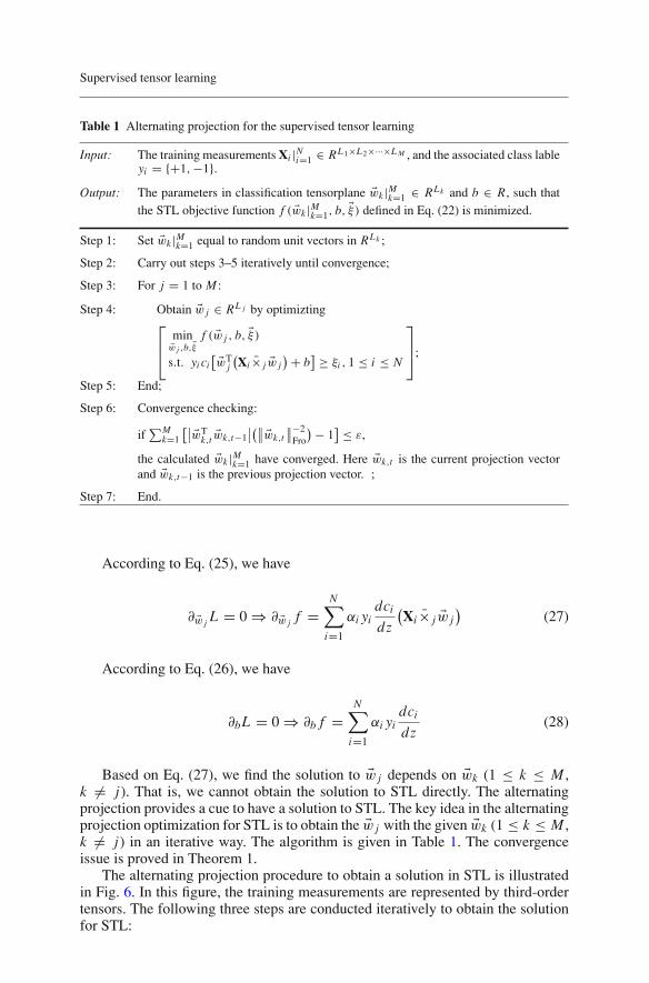
Table 1 Alternating projection for the supervised tensor learning

Input: The training measurements Xi |Ni=1 ∈ RL1×L2×···×L M , and the associated class lable

yi = {+1, −1}.Output: The parameters in classification tensorplane �wk |M

k=1 ∈ RLk and b ∈ R, such thatthe STL objective function f ( �wk |M

k=1, b, �ξ) defined in Eq. (22) is minimized.

Step 1: Set �wk |Mk=1 equal to random unit vectors in RLk ;

Step 2: Carry out steps 3–5 iteratively until convergence;

Step 3: For j = 1 to M :

Step 4: Obtain �w j ∈ RL j by optimizting⎡

⎢⎣

min�w j ,b,�ξ

f ( �w j , b, �ξ)

s.t. yi ci[ �wT

j

(Xi × j �w j

)+ b] ≥ ξi , 1 ≤ i ≤ N

⎤

⎥⎦;

Step 5: End;

Step 6: Convergence checking:

if∑M

k=1

[∣∣ �wT

k,t �wk,t−1∣∣(∥∥ �wk,t

∥∥−2

Fro

)− 1] ≤ ε,

the calculated �wk |Mk=1 have converged. Here �wk,t is the current projection vector

and �wk,t−1 is the previous projection vector. ;

Step 7: End.

According to Eq. (25), we have

∂ �w j L = 0 ⇒ ∂ �w j f =N∑

i=1

αi yidci

dz

(Xi × j �w j

)(27)

According to Eq. (26), we have

∂b L = 0 ⇒ ∂b f =N∑

i=1

αi yidci

dz(28)

Based on Eq. (27), we find the solution to �w j depends on �wk (1 ≤ k ≤ M ,k �= j). That is, we cannot obtain the solution to STL directly. The alternatingprojection provides a cue to have a solution to STL. The key idea in the alternatingprojection optimization for STL is to obtain the �w j with the given �wk (1 ≤ k ≤ M ,k �= j) in an iterative way. The algorithm is given in Table 1. The convergenceissue is proved in Theorem 1.

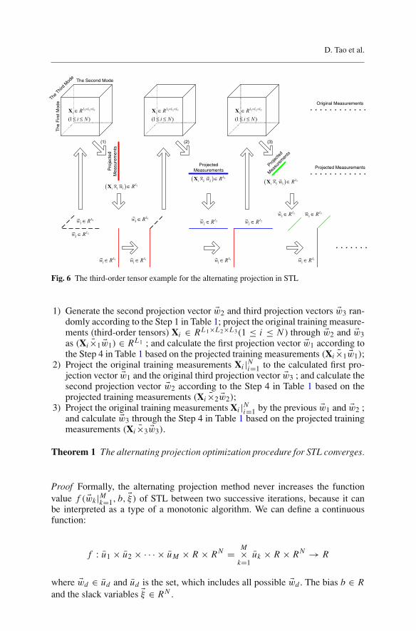
The alternating projection procedure to obtain a solution in STL is illustratedin Fig. 6. In this figure, the training measurements are represented by third-ordertensors. The following three steps are conducted iteratively to obtain the solutionfor STL:

D. Tao et al.

( ) 11 1

Li w R× ∈X

22

Lw R∈

33

Lw R∈

11

Lw R∈

(1)

11

Lw R∈

33

Lw R∈

( ) 22 2

Li w R× ∈X

22

Lw R∈

1 2 3

(1 )

L L Li R

i N

× ×∈≤ ≤

X

The

Firs

t Mod

e

The Second Mode

TheThir

d M

ode

1 2 3

(1 )

L L Li R

i N

× ×∈≤ ≤

X

(2)

Pro

ject

ed

Mea

sure

men

ts1 2 3

(1 )

L L Li R

i N

× ×∈≤ ≤

X

Projected Measurements

11

Lw R∈

22

Lw R∈

(3)

Projec

ted

Mea

sure

men

ts

( ) 33 3

Li w R× ∈X

33

Lw R∈ 33

Lw R∈

11

Lw R∈

Original Measurements

Projected Measurements

Fig. 6 The third-order tensor example for the alternating projection in STL

1) Generate the second projection vector �w2 and third projection vectors �w3 ran-domly according to the Step 1 in Table 1; project the original training measure-ments (third-order tensors) Xi ∈ RL1×L2×L3 (1 ≤ i ≤ N ) through �w2 and �w3as (Xi ×1 �w1) ∈ RL1 ; and calculate the first projection vector �w1 according tothe Step 4 in Table 1 based on the projected training measurements (Xi ×1 �w1);

2) Project the original training measurements Xi |Ni=1 to the calculated first pro-

jection vector �w1 and the original third projection vector �w3 ; and calculate thesecond projection vector �w2 according to the Step 4 in Table 1 based on theprojected training measurements (Xi ×2 �w2);

3) Project the original training measurements Xi |Ni=1 by the previous �w1 and �w2 ;

and calculate �w3 through the Step 4 in Table 1 based on the projected trainingmeasurements (Xi ×3 �w3).

Theorem 1 The alternating projection optimization procedure for STL converges.

Proof Formally, the alternating projection method never increases the functionvalue f ( �wk |M

k=1, b, �ξ) of STL between two successive iterations, because it canbe interpreted as a type of a monotonic algorithm. We can define a continuousfunction:

f : u1 × u2 × · · · × uM × R × RN = M×k=1

uk × R × RN → R

where �wd ∈ ud and ud is the set, which includes all possible �wd . The bias b ∈ Rand the slack variables �ξ ∈ RN .


With the definition, f has M different mappings:

g( �w∗d , b∗

d , �ξ∗d )

�= arg min�ud∈ud ,b,�ξ

f(

�wd∣∣Md=1, b, �ξ

)

= arg min�ud∈ud ,b,�ξ

f(

�wd , b, �ξ ; �wl∣∣d−1l=1 , �wl

∣∣Ml=d+1

),

The mapping can be calculated with the given �wl |d−1l=1 in the t th iteration and

�wl |Ml=d+1 in the (t − 1)th iteration of the for-loop in Step 4 in Table 1.

If each ud for all d ∈ {1, 2, . . . M} is closed, each g( �w∗d , b∗

d , �ξ∗d ) for all d ∈

{1, 2, . . . M} is closed.Given an initial �wd ∈ ud (1 ≤ d ≤ M ), the alternating projection generates a

sequence of items { �w∗d,t , b∗

d,t ,�ξ∗

d,t ; 1 ≤ d ≤ M} via

g(

�w∗d,t , b∗

d,t ,�ξ∗

d,t

)= arg min

�ud∈ud ,b,�ξf(

�wd , b, �ξ ; �wl,t∣∣d−1l=1 , �wl,t−1

∣∣Ml=d+1

)

with each d ∈ {1, 2, · · · M}. The sequence has the following relationship:

a1 = f ( �w∗1,1, b∗

1,1,�ξ∗

1,1) ≥ f ( �w∗2,1, b∗

2,1,�ξ∗

2,1)

≥ · · · ≥ f ( �w∗M,1, b∗

M,1,�ξ∗

M,1) ≥ f ( �w∗1,2, b∗

1,2,�ξ∗

1,2)

≥ · · · ≥ f ( �w∗1,t , b∗

1,t ,�ξ∗

1,t ) ≥ f ( �w∗2,t , b∗

2,t ,�ξ∗

2,t )

≥ · · · ≥ f ( �w∗1,T , b∗

1,T , �ξ∗1,T ) ≥ f ( �w∗

2,T , b∗2,T , �ξ∗

2,T )

≥ · · · ≥ f ( �w∗M,T , b∗

M,T , �ξ∗M,T ) = a2.

where T → +∞. Here, both a1 and a2 are limited values in the R space. The alter-nating projection in STL can be illustrated by a composition of M subalgorithmsdefined as

�d :(

�wd∣∣Md=1, b, �ξ

)�→

d−1∏

l=1

×l �wl × Map( �wd , b, �ξ)

M∏

l=d+1

×l �wl .

It follows that �.= �1 ◦�2 ◦· · ·◦�M = ◦M

d=1 �d is a closed algorithm when-ever all ud are compact. All subalgorithms g( �w∗

d , b∗d , �ξ∗

d ) decrease the value off , so it should be clear that � is monotonic with respect to f . Consequently,we can say that the alternating projection method to optimize STL defined inEq. (22) converges. ��

6 Supervised tensor learning: Examples

Based on the proposed STL and its alternating projection training algorithm, alarge number of tensor-based learning algorithms can be obtained by combiningSTL with different learning criteria, such as SVM, MPM, FDA, and DML.

D. Tao et al.

Support Vectors

iξ

iξ

Positive Measurement

Negative Measurement

Classification Hyperplane

Margin

Margin Error

Fig. 7 SVM maximizes the margin between the positive and negative training measurements

6.1 Support vector machine versus support tensor machine

SVM [5, 10, 27, 28, 34, 35, 45] finds a classification hyperplane, which maximizesthe margin between the positive measurements and the negative measurements, asshown in Fig. 7.

Suppose there are N training measurements �xi ∈ RL (1 ≤ i ≤ N ) associatedwith the class lables yi ∈ {+1,−1}. The traditional SVM [5, 45], i.e., soft-marginSVM, finds a projection vector �w ∈ RL and a bias b ∈ R through

⎡

⎢⎢⎢⎣

min�w,b,�ξ

JC−SVM( �w, b, �ξ) = 1

2‖ �w‖2

Fro + cN∑

i=1

ξi

s.t.yi [ �wT �xi + b] ≥ 1 − ξi , 1 ≤ i ≤ N�ξ ≥ 0

⎤

⎥⎥⎥⎦

(29)

where �ξ = [ξ1, ξ2, . . . , ξN ]T ∈ RN is the vector of all slack variables to dealwith the linearly nonseparable problem. The ξi (1 ≤ i ≤ N ) is also called themarginal error for the i th training measurement, as shown in Fig. 7. The marginis 2

/‖ �w‖Fro. When the classification problem is linearly separable, we can set�ξ = 0. The decision function for classification is y (�x) = sign[ �wT �x + b].

The Lagrangian of Eq. (29) is

L( �w, b, �ξ, �α, �κ)

= 1

2‖ �w‖2

Fro + cN∑

i=1

ξi −N∑

i=1

αi (yi [ �wT �xi + b] − 1 + ξi ) −N∑

i=1

κiξi

= 1

2�wT �w + c

N∑

i=1

ξi −N∑

i=1

αi yi �wT �xi − b�αT �y +N∑

i=1

αi − �αT�ξ − �κT�ξ

(30)


with Lagrangian multipliers αi ≥ 0, κi ≥ 0 for 1 ≤ i ≤ N . The solution isdetermined by the saddle point of the Lagrangian

max�α,�κ

min�w,b,�ξ

L( �w, b, �ξ, �α, �κ) (31)

This can be achieved by

∂ �w L = 0 ⇒ �w =N∑

i=1

αi yi �xi

∂b L = 0 ⇒ �αT �y = 0 (32)

∂�ξ L = 0 ⇒ c − �α − �κ = 0.

Based on Eq. (32), we can have the dual problem of Eq. (29),⎡

⎢⎢⎢⎢⎣

max�α

JD (�α) = −1

2

N∑

i=1

N∑

j=1

yi y j �xTi �x jαiα j +

N∑

i=1

αi

s.t.�αT �y = 0

0 ≤ �α ≤ c

⎤

⎥⎥⎥⎥⎦

(33)

Set P = [yi y j �xTi �x j ]1≤i, j≤N , �q = �1N×1, A = �y, �b = 0, G =

[IN×N , −IN×N ]T, and �h = [c�1TN×1,

�0TN×1]T in Eq. (17), we can see that the dual

problem of Eq. (29) in SVM is a QP.In the soft-margin SVM defined in Eq. (29), the constant c determines the

tradeoff between 1) maximizing the margin between the positive and negativemeasurements and 2) minimizing the training error. The constant c is not intuitive.Therefore, [28, 27] developed the ν-SVM by replacing the unintuitive parameterc with an intuitive parameter ν as

⎡

⎢⎢⎢⎢⎢⎢⎢⎣

min�w,b,�ξ,ρ

Jν−SVM( �w, b, �ξ, ρ) = 1

2‖ �w‖2

Fro + 1

N

N∑

i=1

ξi − νρ

s.t.

yi [ �wT �xi + b] ≥ ρ − ξi , 1 ≤ i ≤ N

�ξ ≥ 0,

ρ ≥ 0

⎤

⎥⎥⎥⎥⎥⎥⎥⎦

(34)

The significance of ν in ν-SVM defined in Eq. (34) is that it controls the num-ber of support vectors and the marginal errors.

Suykens and Vandewalle [33, 34] simplified the soft-margin SVM as the leastsquares SVM,

⎡

⎣ min�w,b,�ε

JLS−SVM ( �w, b, �ε) = 1

2‖ �w‖2

Fro + γ

2�εT�ε

s.t. yi [ �wT �xi + b] = 1 − εi , 1 ≤ i ≤ N

⎤

⎦ (35)

Here, the penalty γ > 0. There are two different points between the soft-margin SVM defined in Eq. (29) and the least squares SVM defined in Eq. (35): 1)

D. Tao et al.

inequality constraints are replaced by equality constraints; and 2) the loss∑N

i=1 ξi(ξi ≥ 0) is replaced by square loss. The two modifications enable the solution ofthe least-square SVM to be conveniently obtained compared to the soft-marginSVM.

According to the statistical learning theory, we know a learning machine per-forms well when the number of the training measurements is larger than the com-plexity of the model. Moreover, the complexity of the model and the number ofthe parameters to describe the model are always in direct proportion. In com-puter vision research, the objects are usually represented by general tensors andthe number of the training measurements is limited. Therefore, it is reasonable tohave the tensor extension of SVM, i.e., the support tensor machine (STM). Basedon Eq. (29) and STL defined in Eq. (22), it is not difficult to obtain the tensorextension of the soft-margin SVM, i.e., the soft-margin STM.

Suppose we have training measurements Xi ∈ RL1×L2×···×L M (1 ≤ i ≤ N )and their corresponding class labels yi ∈ {+1,−1}. The decision function is amultilinear function y (X) = sign[X∏M

k=1 ×k �wk + b], where the projection vec-tors �wk ∈ RLk (1 ≤ k ≤ M) and the bias b in soft-margin STM are obtained from

⎡

⎢⎢⎢⎢⎢⎢⎢⎢⎣

min�wk |M

k=1,b,�ξJC−STM

(�wk∣∣Mk=1, b, �ξ

)= 1

2

∥∥∥∥

M⊗k=1

�wk

∥∥∥∥

2

Fro+ c

N∑

i=1

ξi

s.t.yi

[

Xi

M∏

k=1

×k �wk + b

]

≥ 1 − ξi , 1 ≤ i ≤ N

�ξ ≥ 0

⎤

⎥⎥⎥⎥⎥⎥⎥⎥⎦

(36)

Here, �ξ = [ξ1, ξ2, . . . , ξN ]T ∈ RN is the vector of all slack variables to dealwith the linearly nonseparable problem.

The Lagrangian for this problem is

L(

�wk∣∣Mk=1, b, �ξ, �α, �κ

)

= 1

2

∥∥∥∥

M⊗k=1

�wk

∥∥∥∥

2

Fro+ c

N∑

i=1

ξi

−N∑

i=1

αi

(

yi

[

Xi

M∏

k=1

×k �wk + b

]

− 1 + ξi

)

−N∑

i=1

κiξi

= 1

2

M∏

k=1

�wTk �wk + c

N∑

i=1

ξi −N∑

i=1

αi yi

(

Xi

M∏

k=1

×k �wk

)

− b�αT �y +N∑

i=1

αi − �αT�ξ − �κT�ξ (37)


with Lagrangian multipliers αi ≥ 0, κi ≥ 0 for 1 ≤ i ≤ N . The solution isdetermined by the saddle point of the Lagrangian

max�α,�κ

min�wk |M

k=1,b,�ξL(

�wk∣∣Mk=1, b, �ξ, �α, �κ

)(38)

This can be achieved by

∂ �w j L = 0 ⇒ �w j = 1k �= j∏

k=1�wT

k �wk

N∑

i=1

αi yi(Xi × j �w j

)

∂b L = 0 ⇒ �αT �y = 0 (39)

∂�ξ L = 0 ⇒ c − �α − �κ = 0

The first equation in Eq. (39) shows that the solution of �w j depends on �wk(1 ≤k ≤ M , k �= j). That is, we cannot obtain the solution for soft-margin STMdirectly. This point has been emphasized in the STL framework. Therefore, weuse the proposed alternating projection method in STL to obtain the solution ofsoft-margin STM. To have the alternating projection method for soft-margin STM,we need to replace the Step 4 in Table 1 by the following optimization problem,

⎡

⎢⎢⎢⎢⎣

min�w j ,b,�ξ

JC−STM( �w j , b, �ξ) = η2

∥∥ �w j

∥∥2

Fro + cN∑

i=1ξi

s.t.yi [ �wT

j

(Xi × j �w j

)+ b] ≥ 1 − ξi , 1 ≤ i ≤ N

�ξ ≥ 0

⎤

⎥⎥⎥⎥⎦

(40)

where η = ∏k �= j1≤k≤M ‖ �wk‖2

Fro.The problem defined in Eq. (40) is the standard soft-margin SVM defined in

Eq. (29).Based on ν-SVM defined in Eq. (34) and STL defined in Eq. (22), we can also

have the tensor extension of the ν-SVM, i.e., ν-STM,

⎡

⎢⎢⎢⎢⎢⎢⎢⎢⎢⎢⎣

min�wk |M

k=1,b,�ξ,ρ

Jν−STM

(�wk∣∣Mk=1, b, �ξ, ρ

)= 1

2

∥∥∥∥

M⊗k=1

�wk

∥∥∥∥

2

Fro+ 1

N

N∑

i=1

ξi − νρ

s.t.

yi[Xi

M∏

k=1

×k �wk + b] ≥ ρ − ξi , 1 ≤ i ≤ N

�ξ ≥ 0, 1 ≤ i ≤ N

ρ ≥ 0

⎤

⎥⎥⎥⎥⎥⎥⎥⎥⎥⎥⎦

(41)

D. Tao et al.

Here, ν ≥ 0 is a constant. The Lagrangian for this problem is

L(

�wk∣∣Mk=1, b, �ξ, ρ, �α, �κ, τ

)

= 1

2

∥∥∥∥

M⊗k=1

�wk

∥∥∥∥

2

Fro+ 1

N

N∑

i=1

ξi − νρ − τρ

−N∑

i=1

αi

(

yi

[

Xi

M∏

k=1

×k �wk + b

]

− ρ + ξi

)

− �κT�ξ

= 1

2

M∏

k=1

�wTk �wk + 1

N

N∑

i=1

ξi −N∑

i=1

αi yi

(

Xi

M∏

k=1

×k �wk

)

− b�αT �y + ρ

N∑

i=1

αi − �αT�ξ − �κT�ξ − νρ − τρ, (42)

with Lagrangian multipliers τ ≥ 0 and αi ≥ 0, κi ≥ 0 for 1 ≤ i ≤ N . Thesolution is determined by the saddle point of the Lagrangian

max�α,�κ,τ

min�wk |M

k=1,b,�ξ,ρ

L(

�wk∣∣Mk=1, b, �ξ, ρ, �α, �κ, τ

)(43)

Similar to the soft-margin STM, the solution of �w j depends on �wk (1 ≤ k ≤M , k �= j), because

∂ �w j L = 0 ⇒ �w j = 1k �= j∏

k=1�wT

k �wk

N∑

i=1

αi yi(Xi × j �w j

)(44)

Therefore, we use the proposed alternating projection method in STL to obtainthe solution of ν-STM. To have the alternating projection method for ν-STM, weneed to replace the Step 4 in Table 1 by the following optimization problem,

⎡

⎢⎢⎢⎢⎢⎢⎢⎢⎣

min�w j ,b,�ξ,ρ

Jν−STM( �w j , b, �ξ, ρ

) = η

2

∥∥ �w j

∥∥2

Fro + 1

N

N∑

i=1

ξi − νρ

s.t.

yi

[�wT

j

(Xi × j �w j

)+ b]

≥ ρ − ξi , 1 ≤ i ≤ N

�ξ ≥ 0

ρ ≥ 0

⎤

⎥⎥⎥⎥⎥⎥⎥⎥⎦

(45)


Fro.The problem defined in Eq. (45) is the standard ν-SVM defined in Eq. (34).Based on the least squares SVM defined in Eq. (35) and the STL defined in

Eq. (22), we can also have the tensor extension of the least-square SVM, i.e.,


least-square STM,⎡

⎢⎢⎢⎢⎣

min�wk |M

k=1,b,�εJL S−ST M

(�wk∣∣Mk=1, b, �ε

)= 1

2

∥∥∥∥

M⊗k=1

�wk

∥∥∥∥

2

Fro+ γ

2�εT�ε

s.t. yi

[

Xi

M∏

k=1

×k �wk + b

]

= 1 − εi , 1 ≤ i ≤ N

⎤

⎥⎥⎥⎥⎦

(46)

where γ > 0 is a constant. Similar to the soft-margin STM and ν-STM, there isno closed-form solution for least squares STM. We use the alternating projectionmethod in STL to obtain the solution of the least squares STM. To have the alter-nating projection method for the least squares STM, we need to replace the Step4 in Table 1 by the following optimization problem,

⎡

⎣min�w j ,b,�ε

JL S−ST M

(�wk∣∣Mk=1, b, �ε

)= η

2

∥∥ �w j

∥∥2

Fro + γ

2�εT�ε

s.t. yi[ �wT

j

(Xi × j �w j

)+ b] = 1 − εi , 1 ≤ i ≤ N

⎤

⎦ (47)


Fro.

Theorem 2 In STM, the decision function is defined by a multilinear function

y (X) = sign[X∏Mk=1 ×k �wk + b] with ‖ M⊗

k=1�wk‖2

Fro ≤ �2and ‖X‖2Fro ≤ R2. Let

ρ > 0 and ν is the fraction of training measurements with margin smaller thanρ/|�|. When STM is obtained from N training measurements ‖Xi‖2

Fro ≤ R2

(1 ≤ i ≤ N), sampled from a distribution P with probability at least 1 − δ(0 < δ < 1), the misclassification probability of a test measurement sampled fromP is bounded by

ν +√

λ

N

(R2�2

ρ2ln2 N + ln

1

δ

)

(48)

where λ is a universal constant.

Proof This is a direct conclusion from the theorem on the margin error boundintroduced in [28]. More information about other error bounds in SVM can befound in [2]. ��

6.2 Minimax probability machine versus tensor minimax probability machine

The minimax probability machine (MPM) [16, 31] has become popular. It is re-ported to outperform the conventional SVM consistently and, therefore, has at-tracted attention as a promising supervised learning algorithm. MPM focuses onfinding a decision hyperplane, which is H ( �w, b) = {�x | �wT �x + b = 0}, to separatethe positive measurements from the negative measurements (a binary classificationproblem) with maximal probability with respect to all distributions modeled bygiven means and covarainces, as shown in Fig. 8. MPM maximizes the probabilityof correct classification rate (classification accuracy) on the future measurements.

D. Tao et al.




( ),m+ +Σ

( ),m− −Σ

Intersection Point

Fig. 8 MPM separates the positive measurements from the negative measurements by maxi-mizing the probability of the correct classification for the future measurements. The intersectionpoint minimizes the maximum of the Mahalanobis distances of the positive and negative mea-surements, i.e., it has the same Mahalanobis distances to the mean of the positive measurementsand the mean of the negative measurements

For Gaussian-distributed measurements, it minimizes the maximum of the Maha-lanobis distances of the positive measurements and the negative measurements.With the given positive measurements �xi (yi = +1) and negative measurements�xi (yi = −1), MPM is defined as,

⎡

⎢⎢⎢⎣

max�w,b,δ

JMPM ( �w, b, δ) = δ

s.t.inf

�xi (yi =+1)∼( �m+,�+)Pr{ �wT �xi + b ≥ 0

} ≥ δ

inf�xi (yi =−1)∼( �m−,�−)

Pr{ �wT �xi + b ≤ 0

} ≥ δ

⎤

⎥⎥⎥⎦

(49)

Here, the notation �xi (yi = +1) ∼ ( �m+, �+) means the class distribution ofthe positive measurements has the mean �m+ and covariance �+. So does the no-tation �xi (yi = −1) ∼ ( �m−, �−). The classification decision function is given byy (�x) = sign[ �wT �x + b].

Recently, based on the powerful Marshall and Olkin’s theorem [20], Popescuand Bertsimas [23] proved a probability bound,

sup�x∼( �m,�)

Pr {�x ∈ S} = 1

1 + d2with d2 = inf

�x∈S(�x − �m)T �−1 (�x − �m) (50)

where �x stands for a random vector, S is a given convex set, and the supremumis taken over all distributions for �x with the mean value as �m and the covariancematrix �. Based on this result, Lanckriet et al. [16] reformulated Eq. (49) as:

⎡

⎢⎢⎢⎣

max�w,b,κ

JMPM ( �w, b, κ) = κ

s.t.�wT �m+ + b ≥ +κ

√ �wT�+ �w, yi = +1

�wT �m− + b ≤ −κ√ �wT�− �w, yi = −1

⎤

⎥⎥⎥⎦

(51)


where the constraint functions in Eq. (51) are second-order cone functions. ThereMPM is an SOCP. This problem can be further simplified as

[min

�wJMPM ( �w) = √ �wT�+ �w +√ �wT�− �w

s.t. �wT ( �m+ − �m−) = 1

]

(52)

where b is determined by

b∗ = ( �w∗)T �m+ −√

( �w∗)T �+ ( �w∗)√

( �w∗)T �+ ( �w∗) +√

( �w∗)T �− ( �w∗)

(53)

In computer vision research, many objects are represented by tensors. Tomatch the input requirments in MPM, we need to vectorize the tensors to vectors.When the training measurements are limited, the vectorization will be a disaster.This is because MPM meets the matrix singular problem seriously (the ranks of�+ and �− are deficient). To reduce this problem, we propose the tensor exten-sion of MPM, i.e., tensor MPM (TMPM). TMPM is a combination of MPM andSTL.

Suppose we have the training measurements Xi ∈ RL1×L2×···×L M (1 ≤ i ≤N ) and their corresponding class labels yi ∈ {+1,−1}. The decision functionis a multilinear function y (X) = sign[X∏M

k=1 ×k �wk + b], where the projectionvectors �wk ∈ RLk (1 ≤ k ≤ M) and the bias b in TMPM are obtained from

⎡

⎢⎢⎢⎢⎢⎢⎢⎢⎢⎣

max�wk |M

k=1,b,κ

JMPM

(�wk∣∣Mk=1, b, κ

)= κ

s.t.

1N+

(N∑

i=1

[

I(yi = +1)Xi

M∏

k=1

×k �wk

])

+b ≥ +κ sup1≤l≤M

√�wT

l �+;l �wl

1N−

(N∑

i=1

[

I(yi = −1)Xi

M∏

k=1

×k �wk

])

+b ≤ −κ sup1≤l≤M

√�wT

l �−;l �wl

⎤

⎥⎥⎥⎥⎥⎥⎥⎥⎥⎦

(54)where �+;l is the covariance matrix of the projected measurements (Xi ×−l �wl)for all yi = +1 and �−;l is the covariance matrix of the projected measurements(Xi ×−l �wl) for all yi = −1. The function I(yi = +1) is 1 if yi is +1, otherwise0. The function I(yi = −1) is 1 if yi is −1, otherwise 0. This problem can besimplified as

⎡

⎢⎢⎢⎢⎢⎢⎢⎢⎢⎣

max�wk |M

k=1,b,κ

JMPM

(�wk∣∣Mk=1, b, κ

)= κ

s.t.

M+M∏

k=1

×k �wk + b ≥ +κ sup1≤l≤M

√�wT

l �+;l �wl

M−M∏

k=1

×k �wk + b ≤ −κ sup1≤l≤M

√�wT

l �−;l �wl

⎤

⎥⎥⎥⎥⎥⎥⎥⎥⎥⎦

(55)

D. Tao et al.

where M+ = (1/

N+)∑N

i=1 [I(yi = +1)Xi ], M− = (1/

N−)∑N

i=1[I(yi = −1)Xi ], N+ (N−) is the number of the positive (negative) measurements.

The Lagrangian for this problem is

L(

�wk |Mk=1, b, κ, �α

)

= − κ − α1

(

M+M∏

k=1

×k �wk + b − κ sup1≤l≤M

√�wT

l �+;l �wl

)

+ α2

(

M−M∏

k=1

×k �wk + b + κ sup1≤l≤M

√�wT

l �−;l �wl

)

= − κ − α1b

N++ α2b

N−− α1M+

M∏

k=1

×k �wk + α2M−M∏

k=1

×k �wk

+ α1κ

N+sup

1≤l≤M

√�wT

l �+;l �wl + α2κ

N−sup

1≤l≤M

√�wT

l �−;l �wl (56)

with Lagrangian multipliers αi ≥ 0 (i = 1, 2). The solution is determined by thesaddle point of the Lagrangian

max�α

min�wk

∣∣M

k=1,b,κ

L(

�wk |Mk=1, b, κ, �α

)(57)

This can be achieved by setting ∂ �w j L = 0, ∂b L = 0, and ∂κ L = 0. It isnot difficult to find that the solution of �w j depends on �wk (1 ≤ k ≤ M , k �=j). Therefore, there is no closed-form solution for TMPM. We use the proposedalternating projection method in STL to obtain the solution of TMPM. To have thealternating projection method for TMPM, we need to replace the Step 4 in Table1 by the following optimization problem,

⎡

⎢⎢⎢⎣

max�w j ,b,κ

JMPM( �w j , b, κ) = κ

s.t.�wT

j (M+× j �w j ) + b ≥ +κ√

�wTj �+; j �w j

�wTj (M−× j �w j ) + b ≤ −κ

√�wT

j �−; j �w j

⎤

⎥⎥⎥⎦

(58)

This problem is the standard MPM defined in Eq. (51).

6.3 Fisher discriminant analysis versus tensor fisher discriminant analysis

Fisher discriminant analysis (FDA) [6, 8, 14] as shown in Fig. 9 has been widelyapplied for classification. Suppose there are N training measurements �xi ∈ RL

(1 ≤ i ≤ N ) associated with the class lables yi ∈ {+1,−1}. There are N+ positivetraining measurements and their mean is �m+ = (1/N+)

∑Ni=1 [I(yi = +1)�xi ];

there are N− negative training measurements and their mean can be calculatedfrom �m− = (1/N−)

∑Ni=1

[I(yi = −1)�xi

]; the mean of all training measurements





( ),m+ Σ

( ),m− Σ

Fig. 9 FDA separates the positive measurements from the negative measurements by maximiz-ing the symmetric Kullback–Leibler divergence between the two classes under the assumptionthat the two classes share the same covariance matrix

is �m = (1/N )∑N

i=1 �xi ; and the covariance matrix of all training measurementsis �. FDA finds a direction to separate the class means well while minimizingthe variance of the total training measurements. Therefore, two quantities need tobe defined, which are: 1) the between-class scatter Sb = ( �m2 − �m1) ( �m2 − �m1)

T:measuring the difference between the two classes; and 2) the within-class scatterSw = ∑N

i=1 (�xi − �m) (�xi − �m)2 = N�: the variance of the total training mea-surements. The projection direction �w maximizes

[

max�w

JF D A ( �w) = �wTSb �w�wTSw �w

]

(59)

This problem is simplified as[

max�w

JF D A ( �w) =∥∥ �wT ( �m+ − �m−)

∥∥

√ �wT� �w

]

(60)

According to [37], we know this procedure is equivalent to maximizing thesymmetric Kullback–Leibler divergence (KLD) between the positive and the neg-ative measurements with identical covariances, so that the positive measurementsare separated from the negative measurements. Based on the definition of FDA,we know FDA is a special case of the linear discriminant analysis (LDA).

The linear decision function in FDA is y (�x) = sign[ �wT �x + b], where �w is theeigenvector of �−1 ( �m+ − �m−) ( �m+ − �m−)T associated with the largest eigen-value and the bias b is calculated by

b = N− − N+ − (N+ �m+ + N− �m−)T �wN− + N+

(61)

The significance [6, 9] of FDA is: FDA is Bayes optimal when the two classesare Gaussian distributed with identical covariances.

When objects are represented by tensors, we need to vectorize the tensors tovectors to match the input requirments in FDA. When the training measurementsare limited, the vectorization will be a disaster for FDA. This is because Sw and

D. Tao et al.

Sb are both singular. To reduce this problem, we propose the tensor extension ofFDA, i.e., tensor FDA (TFDA). TFDA is a combination of FDA and STL. More-over, TFDA is a special case of the previous proposed general tensor discriminantanalysis (GTDA) [38].

Suppose we have the training measurements Xi ∈ RL1×L2×···×L M (1 ≤ i ≤N ) and their corresponding class labels yi ∈ {+1,−1}. The mean of the trainingpositive meansurements is M+ = (1/N+)

∑Ni=1 [I(yi = +1)Xi ] ; the mean of the

training negative measurements is given by M− = (1/N−)∑N

i=1 [I(yi = −1)Xi ]; the mean of all training measurements is M = (1/N )

∑Ni=1 Xi ; and N+(N−)

is the number of the positive (negative) measurements. The decision function is amultilinear function y (X) = sign[X∏M

k=1 ×k �wk + b], where the projection vec-tors �wk ∈ RLk (1 ≤ k ≤ M) and the bias b in TFDA are obtained from

⎡

⎢⎣ max

�wk |Mk=1

JTFDA

(�wk∣∣Mk=1

)=

∥∥∥(M+ − M−)

∏Mk=1 ×k �wk

∥∥∥

2

∑Ni=1

∥∥∥(Xi − M)

∏Mk=1 ×k �wk

∥∥∥

2

⎤

⎥⎦ (62)

There is no closed-form solution for TFDA. The alternating projection is ap-plied to obtain the solution for TFDA and we need to replace the Step 4 in Table1 by the following optimization problem,

⎡

⎢⎣max

�w j

JTFDA( �w j ) =∥∥∥ �wT

j

[(M+ − M−

)× j �w j]∥∥∥

2

∑Ni=1

∥∥∥ �wT

j [(Xi − M) × j �w j ]∥∥∥

2

⎤

⎥⎦ (63)

This problem is the standard FDA. When we have the projection vectors�wk |M

k=1, we can obtain the bias b from

b = N− − N+ − (N+M+ + N−M−)∏M

k=1 ×k �wk

N− + N+(64)

6.4 Distance metric learning versus multiple distance metrics learning

Weinberger et al. [49] proposed the distance metric learning (DML) to learn ametric for k-nearest-neighbor (kNN) classification (see Fig. 10). The motivationof DML is simple because the performance of kNN is only related to the metricused for dissimilarity measure. In traditional kNN, this measure is the Euclideanmetric, which fails to capture the statistical charateristics of the training measure-ments. In DML, the metric is obtained to guarantee: 1) k-nearest neighbors of ameasurement have the identical label with the measurement; and 2) measurementswith different lables are separated from the measurement according to marginmaximization.


Margin Margin

Target Neighborhood

Local NeighborhoodBefore After

ix

ix

Similarly Labeled

Differently Labeled

Differently Labeled

Fig. 10 DML obtains a metric to guarantee: 1) k-nearest neighbors of a measurement have theidentical label with the measurement; and 2) measurements with different lables are separatedfrom the measurement according to margin maximization

DML is defined by

⎡

⎢⎢⎢⎢⎢⎢⎢⎢⎢⎢⎢⎢⎢⎢⎢⎢⎣

min�,ξi jl1≤i, j,l≤N

JDML(�, ξi jl) =N∑

i=1

N∑

j=1

ηi j (�xi − �x j )T�(�xi − �x j )

+ cN∑

i=1

N∑

j=1

ηi j (1 − yil) ξi jl

s.t.

(�xi − �xl)T � (�xi − �xl) − (�xi − �x j )

T�(�xi − �x j )

≥ 1 − ξi jl , 1 ≤ i, j, l ≤ N

ξi jl ≥ 0, 1 ≤ i, j, l ≤ N

� ≥ 0

⎤

⎥⎥⎥⎥⎥⎥⎥⎥⎥⎥⎥⎥⎥⎥⎥⎥⎦

(65)

where ηi j = 1 and yi j = 1 mean that �xi and �x j have the same class label, oth-erwise 0. The constraint function � ≥ 0 indicates that the maxtrix � is requiredto be positive semidefinite, so the problem is an SDP. From the learnt distancemetric �, it is direct to have the linear transformation matrix by decomposing� = W TW .

D. Tao et al.

The optimization problem defined in Eq. (65) is equivalent to

⎡

⎢⎢⎢⎢⎢⎢⎢⎢⎢⎣

min�,ξi jl1≤i, j,l≤N

JDML(�, ξi jl) = tr(AT� A) + cN∑

i=1

N∑

j=1


s.t.

BTi jl�Bi jl ≥ 1 − ξi jl , 1 ≤ i, j, l ≤ N

ξi jl ≥ 0, 1 ≤ i, j, l ≤ N

� ≥ 0

⎤

⎥⎥⎥⎥⎥⎥⎥⎥⎥⎦

(66)

where A = [√ηi j (�xi − �x j )]L×N 2 (1 ≤ i, j ≤ N ) and Bi jl =[�xi − �xl , �x j − �xi ]L×2

Suppose we have the training measurements Xi ∈ RL1×L2×···×L M (1 ≤ i ≤N ) and their corresponding class labels yi ∈ {1, 2, . . . , n}. The multiple distancemetrics learning (MDML) learns M metrics �k = W T

k Wk (1 ≤ k ≤ M) forXi |N

i=1 to make the measurements, which have the same (different) labels, and areas close (far) as possible. The MDML is defined as

⎡

⎢⎢⎢⎢⎢⎢⎢⎢⎢⎢⎢⎢⎢⎢⎢⎢⎢⎢⎢⎢⎢⎢⎢⎣

minWk |M

k=1,ξi jl1≤i, j,l≤N

JMDML

(Wk∣∣Mk=1, ξi jl |1≤i, j,l≤N

)

=

⎡

⎢⎢⎢⎢⎢⎣

N∑

i=1

N∑

j=1

ηi j

∥∥∥∥∥(Xi − X j )

M∏

k=1

×k Wk

∥∥∥∥∥

2

Fro

+cN∑

i=1

N∑

j=1


⎤

⎥⎥⎥⎥⎥⎦

s.t.

∥∥∥∥∥(Xi − Xl)

M∏

k=1

×k Wk

∥∥∥∥∥

2

Fro

−∥∥∥∥∥(Xi − X j )

M∏

k=1

×k Wk

∥∥∥∥∥

2

Fro

≥ 1 − ξi jl

ξi jl ≥ 0, 1 ≤ i, j, l ≤ N

W Tk Wk ≥ 0, 1 ≤ k ≤ M

⎤

⎥⎥⎥⎥⎥⎥⎥⎥⎥⎥⎥⎥⎥⎥⎥⎥⎥⎥⎥⎥⎥⎥⎥⎦

(67)As described in STL framework, there is also no closed-form solution for

MDML. The alternating projection method is applied to obtain the solution for


MDML and we need to replace Step 4 in Table 1 by the following optimizationproblem,

⎡

⎢⎢⎢⎢⎢⎢⎢⎢⎢⎢⎢⎢⎢⎢⎢⎢⎣

minWp,ξi jl1≤i, j,l≤N

JMDML(Wp, ξi jl |1≤i, j,l≤N )

= tr(

ATp�p Ap

)+ c

N∑

i=1

N∑

j=1


s.t.

∥∥∥∥∥(Xi − Xl)

M∏

k=1

×k Wk

∥∥∥∥∥

2

Fro

−∥∥∥∥∥

(Xi − X j

) M∏

k=1

×k Wk

∥∥∥∥∥

2

Fro

≥ 1 − ξi jl

ξi jl ≥ 0, 1 ≤ i, j, l ≤ N

W Tk Wk ≥ 0, 1 ≤ k ≤ M

⎤

⎥⎥⎥⎥⎥⎥⎥⎥⎥⎥⎥⎥⎥⎥⎥⎥⎦

(68)Here,

Ap =N∑

i=1

N∑

j=1

√ηi j matp((Xi − X j )×pWp) (69)

and

Bi jl;p = matp((X j − Xl)×pWp) (70)

This is because ‖(Xi − Xl)∏M

k=1 ×k Wk‖2Fro = tr(matTj ((Xi − Xl)× j W j )� j

mat j ((Xi − Xl)× j W j ))

Derivation

∥∥∥∥∥(Xi − Xl)

M∏

k=1

×k Wk

∥∥∥∥∥

2

Fro

=[[(

(Xi − Xl)

M∏

k=1

×k Wk

)

⊗(

(Xi − Xl)

M∏

k=1

×k Wk

)

; (1 : M) (1 : M)

]]

= tr[[([(Xi − Xl)× j W j ] × j W j ) ⊗ ([(Xi − Xl)× j W j ]× j W j ); (1 : M) (1 : M)]]

= tr(W j [[[(Xi − Xl)× j W j ] ⊗ [(Xi − Xl)× j W j ]; ( j)( j)]]W Tj )

= tr(W j mat j ((Xi − Xl)× j W j )matTj ((Xi − Xl)× j W j )W Tj )

= tr(matTj ((Xi − Xl)× j W j )W Tj W j mat j ((Xi − Xl)× j W j ))

= tr(matTj ((Xi − Xl)× j W j )� j mat j ((Xi − Xl)× j W j )).

This problem defined in Eq. (68) is the standard DML.

D. Tao et al.

1 2 3, 1

(1 )

L L Li r R

i N

× ×− ∈

≤ ≤X

1 2 3

, 1

(1 )

L L Li r R

i N

× ×− ∈

≤ ≤

X 3

, 1 , 11

i r k rk

wλ − ⊗ −=

∏1 2 3

,

(1 )

L L Li r R

i N

× ×∈≤ ≤

X

1, 1rw −2, 1rw −

1, 1rw −

3, 1rw −

1×

3×

2×2, 1rw −

3, 1rw −

, 1i tλ −

Fig. 11 Iterative feature extraction model for third-order tensors

7 Iterative feature extraction model based on supervised tensor learning

The iterative feature extraction model (IFEM) based on STL is an extension ofthe STL framework for feature extraction and its procedure is similar to the recur-sive rank-one tensor approximation developed by Shashua and Levin in [29]. Anexample of IFEM is given in [39].

Suppose we have the training measurements Xi ∈ RL1×L2×···×L M (1 ≤ i ≤N ) and their corresponding class labels yi ∈ {+1, −1}. IFEM is defined by

Xi,r = Xi,r−1 − λi,r−1

M∏

k=1

×k �wk,r−1 (71)

λi,r−1 = Xi,r−1

M∏

k=1

×k ( �wk,r−1)T (72)

⎡

⎢⎢⎢⎣

min�wk,r |M

k=1,b,�ξf(

�wk,r∣∣Mk=1, b, �ξ

)

s.t. yi ci

(

Xi,r

M∏

k=1

×k �wk,r + b

)

≥ ξi , 1 ≤ i ≤ N

⎤

⎥⎥⎥⎦

(73)

where Xi,1 = Xi and λi,0 = 0. The λi,r |Rr=1 (R is the number of the extracted

features in IFEM) is used to represent the original tensor Xi .From the definition of IFEM, which is defined by Eqs. (71)–(73), we know

that IFEM can be calculated by a greedy approach. The calculation of Xi,r |Ni=1


Fig. 12 Attention model for image representation

is based on the given Xi,r−1|Ni=1 and �wk,r−1|M

k=1. With the given Xi,r−1|Ni=1 and

�wk,r−1|Mk=1, we can calculate λi,r−1 via Eq. (72). The projection vectors �wk,r |M

k=1can be obtained by optimizing Eq. (73) through the alternating projection methodin Table 1. The flowchart of the algorithm for feature extraction for third-ordertensors is illustrated in Fig. 11.

With IFEM, we can obtain �wk,r |1≤r≤R1≤k≤M iteratively. The coordinate values

λi,r |Rr=1 can represent the original tensor Xi . For example, in nearest neighbor-

based recognition, the prototype tensor Xp for each individual class in the databaseand the testing tensor Xt to be classified are projected onto the bases to get the pro-totype vector λp,r |R

r=1 and the testing vector λt,r |Rr=1. The testing tensor class is

found by minimizing the Euclidean distance ε =√∑R

r=1 (λt,r − λp,r )2 over p.

8 Experiment

In this section, we provide experiments for image classification with TMPM andMPM. The experiments demonstrate that tensor representation can reduce theoverfitting problem, i.e., STL is a powerful tool for classification in computervision research.

8.1 TMPM for image classification

To categorize images into groups based on their semantic contents is very impor-tant and challenging. Its fundamental task is the binary classification and thus a

D. Tao et al.

hierarchical structure can be built according to a series of binary classifiers. As aresult, this semantic image classification can make the growing image repositorieseasy to search and browse [24, 25]. The image semantic classification is also ofgreat help for many applications.

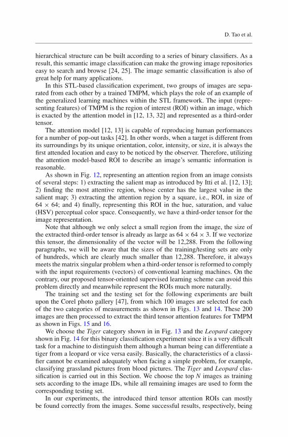
In this STL-based classification experiment, two groups of images are sepa-rated from each other by a trained TMPM, which plays the role of an example ofthe generalized learning machines within the STL framework. The input (repre-senting features) of TMPM is the region of interest (ROI) within an image, whichis exacted by the attention model in [12, 13, 32] and represented as a third-ordertensor.

The attention model [12, 13] is capable of reproducing human performancesfor a number of pop-out tasks [42]. In other words, when a target is different fromits surroundings by its unique orientation, color, intensity, or size, it is always thefirst attended location and easy to be noticed by the observer. Therefore, utilizingthe attention model-based ROI to describe an image’s semantic information isreasonable.

As shown in Fig. 12, representing an attention region from an image consistsof several steps: 1) extracting the salient map as introduced by Itti et al. [12, 13];2) finding the most attentive region, whose center has the largest value in thesalient map; 3) extracting the attention region by a square, i.e., ROI, in size of64 × 64; and 4) finally, representing this ROI in the hue, saturation, and value(HSV) perceptual color space. Consequently, we have a third-order tensor for theimage representation.

Note that although we only select a small region from the image, the size ofthe extracted third-order tensor is already as large as 64 × 64 × 3. If we vectorizethis tensor, the dimensionality of the vector will be 12,288. From the followingparagraphs, we will be aware that the sizes of the training/testing sets are onlyof hundreds, which are clearly much smaller than 12,288. Therefore, it alwaysmeets the matrix singular problem when a third-order tensor is reformed to complywith the input requirements (vectors) of conventional learning machines. On thecontrary, our proposed tensor-oriented supervised learning scheme can avoid thisproblem directly and meanwhile represent the ROIs much more naturally.

The training set and the testing set for the following experiments are builtupon the Corel photo gallery [47], from which 100 images are selected for eachof the two categories of measurements as shown in Figs. 13 and 14. These 200images are then processed to extract the third tensor attention features for TMPMas shown in Figs. 15 and 16.

We choose the Tiger category shown in in Fig. 13 and the Leopard categoryshown in Fig. 14 for this binary classification experiment since it is a very difficulttask for a machine to distinguish them although a human being can differentiate atiger from a leopard or vice versa easily. Basically, the characteristics of a classi-fier cannot be examined adequately when facing a simple problem, for example,classifying grassland pictures from blood pictures. The Tiger and Leopard clas-sification is carried out in this Section. We choose the top N images as trainingsets according to the image IDs, while all remaining images are used to form thecorresponding testing set.

In our experiments, the introduced third tensor attention ROIs can mostlybe found correctly from the images. Some successful results, respectively, being


Fig. 13 Example images from the Tiger category

extracted from the Tiger category and the Leopard category, are shown in Figs. 15and 16. By this means, the underlying data structures are kept well for the nextclassification step. However, we should note that the attention model sometimescannot depict the semantic information of an image. This is mainly because theattention model always locates the region that is different from its surroundingsand thus might be cheated when some complex or bright background exists. Someunsuccessful ROIs can also be found from Figs. 15 and 16. It should be empha-sized that to keep the following comparative experiments fair and automatic, thesewrongly extracted ROIs are not excluded from the training sets. Therefore, it is an-other challenge for both the conventional learning machine (MPM) and our newlyproposed one (TMPM).

D. Tao et al.

Fig. 14 Example images from the leopard category

We carried out the binary classification (Tiger and Leopard) experiments uponthe above training and testing sets. The proposed TMPM is compared with theMPM. The experimental results are shown in Table 2. Error rates for both trainingand testing are reported according to the increasing size of the training set (STS)from 5 to 30 with a step 5.

From the training error rates in Table 2, it can be seen that the traditionalmethod (MPM) cannot learn a satisfying model for classification when the sizeof the measurement set is much smaller than the features’ dimensionality in thelearning state. However, the machine learning algorithm under the proposed STLframework (TMPM) has a good characteristic on the volume control according tothe computational learning theory and its real performances.


Fig. 15 One hundred ROIs in the Tiger category

Also from Table 2, based on the testing error rates of the comparative ex-periments, the proposed TMPM algorithm is demonstrated to be more effectiveto represent the intrinsic discriminative information (in the form of the third-order ROIs). TMPM learns a better classification model for future data classifi-cation than MPM and thus has a satisfactory performance on the testing set. It is

Table 2 TMPM versus MPM

Training error rate Testing error rate

STS TMPM MPM TMPM MPM

5 0.0000 0.4000 0.4600 0.505010 0.0000 0.5000 0.4250 0.490015 0.0667 0.4667 0.3250 0.415020 0.0500 0.5000 0.2350 0.480025 0.0600 0.4800 0.2400 0.465030 0.1167 0.5000 0.2550 0.4600

D. Tao et al.

Fig. 16 One hundred ROIs in the Leopard category

observed that the TMPM error rate is a decreasing function of the size of the train-ing set. This is actually consistent with the statistical learning theory.

We also evaluate TMPM as a sample algorithm of the proposed STL frame-work. Two important issues in machine learning are studied, namely, the conver-gence property and the insensitiveness to the initial values.

Fig. 17 shows that as a sample algorithm of the STL framework, TMPM con-verges efficiently by the alternating projection method. Usually, 20 iterations areenough to achieve the convergence.

Three subfigures in the left column of Fig. 17 show tensor-projected positionvalues of the original general tensors with an increasing number of learning it-erations using 10, 20, and 30 training measurements for each class, respectively,from top to bottom. We find that the projected values converge at stable values.Three subfigures in the right column of Fig. 17 show the training error rates andthe testing error rates according to the increasing number of learning iterationsby 10, 20, and 30 training measurements for each class, respectively, from top tobottom.


0 10 20 30 40 50 60 70 80 90 100−4

−3.5

−3

−2.5

−2

−1.5

−1

Number of Iterations

Pos

ition

Tensor MPM is convergence on the training data

0 10 20 30 40 50 60 70 80 90 100−0.1

−0.05

0

0.05

0.1

0.15

0.2

0.25

0.3

0.35

0.4


Err

or R

ate

Training and Tesing Error Rate vs. Number of Iterations

Training ErrorTesting Error

0 10 20 30 40 50 60 70 80 90 100−6

−5

−4

−3

−2

−1

0


Pos

ition


0 10 20 30 40 50 60 70 80 90 1000

0.05

0.1

0.15

0.2

0.25

0.3

0.35

0.4


Err

or R

ate

Training and Tesing Error Rate vs. Number of Iterations

Training ErrorTesting Error

0 10 20 30 40 50 60 70 80 90 100−6

−5

−4

−3

−2

−1

0

1

2


Pos

ition


0 10 20 30 40 50 60 70 80 90 1000.1

0.15

0.2

0.25

0.3

0.35


Err

or R

ate

Training and Testing Error Rate vs. Number of Iterations

Training ErrorTesing Error

Fig. 17 TMPM converges effectively

Based on all subfigures in Fig. 17, it can be found that the training error andthe testing error are converged at some stable values. Therefore, upon these obser-vations, we also empirically justified the convergence of the alternating projectionmethod for TMPM. The theoretical proof is given in Theorem 1.

Many learning algorithms converge at different destinations with differentinitial parameter values. This is the so-called local minimal problem. However,the developed TMPM does not slump into this local minimal problem, which isdemonstrated by a set of experiments (with 100 different initial parameters, 10learning iterations, and 20 training measurements). From the theoretical view, the

D. Tao et al.

Fig. 18 TMPM is stable with different initial values

TMPM is also a convex optimization problem, so the solution to TMPM is unique.Figure 18 shows this point. The training error rates and the testing error rates arealways 0.05 and 0.235, respectively.

9 Conclusion

In this paper, the vector-based learning is extended to accept tensors as input. Theresult is the supervised tensor learning (STL) framework, which is the multilinearextension of the convex optimization-based learning. To obtain the solution of anSTL-based learning algorithm, the alternating projection method is designed.

Based on STL and its alternating projection optimization algorithm, we il-lustrate several examples. That is, we extend the soft-margin support vector ma-chines (SVM), the ν-SVM, the least squares SVM, the minimax probability ma-chine (MPM), the Fisher discriminant analysis (FDA), the distance metric learning(DML) to their tensor versions, which are the soft-margin support tensor machine(STM), the ν-STM, the least squares STM, the tensor MPM (TMPM), the tensorFDA (TFDA), and the multiple distance metrices learning (MDML). Based onSTL, we also introduce a method for feature extraction through an iterative way,i.e., we develop the iterative feature extraction model (IFEM). Finally, we imple-ment TMPM for image classification. By comparing TMPM with MPM, we knowTMPM reduces the overfitting problem in MPM.

Acknowledgements We thank the editors and anonymous reviewers for their very useful com-ments and suggestions.


References

1. Amini R, Gallinari P (2005) Semi-supervised learning with an imperfect supervisor. KnowlInf Syst 8(4):385–413

2. Bartlett P, Shawe-Taylor J (1998) Generalization performance of support vector machinesand other pattern classifiers. In: Scholkopf B, Burges CJ, Smola AJ (eds) Advances in kernelmethods—support vector learning. MIT Press, Cambridge, MA

3. Boyd S, Vandenberghe L (2004) Convex optimization. Cambridge University Press,Cambridge, UK

4. Boyd S, Kim SJ, Vandenberghe L, Hassibi A (2006) A tutorial on geometric programming.Optim Eng

5. Burges JC (1998) A tutorial on support vector machines for pattern recognition. Data MinKnowl Discov 2(2):121–167

6. Duda RO, Hart PE, Stork DG (2001) Pattern classification. Wiley, New York7. Etemad K, Chellappa R (1998) Discriminant analysis for recognition of human face images.

J Opt Soc Am A 14(8):1,724–1,7338. Fisher RA (1938) The statistical utilization of multiple measurements. Ann Eugenics

8:376–3869. Fukunaga K (1990) Introduction to statistical pattern recognition, 2nd edn. Academic, New

York10. Fung G, Mangasarian OL (2001) Proximal support vector machine classifiers. In: Proceed-

ings of the 7th ACM SIGKDD international conference on knowledge discovery and datamining, San Francisco, CA, pp 77–86

11. Girgensohn A, Foote J (1999) Video classification using transform coefficients. In: Pro-ceedings of the IEEE international conference on acoustics, speech, and signal processing,vol 6, pp 3045–3048

12. Itti L, Koch C, Niebur E (1998) A model of saliency-based visual attention for rapid sceneanalysis. IEEE Trans Pattern Anal Mach Intell 20(11):1,254–1,259

13. Itti L, Koch C (2001) Computational modeling of visual attention. Nat Rev Neurosci2(3):194–203

14. Kim SJ, Magnani A, Boyd S (2005) Robust Fisher discriminant analysis. In: Advances inneural information processing systems. Vancouver and Whistler, British Columbia, Canada

15. Lanckriet G, Cristianini N, Bartlett P, Ghaoui L, Jordan M (2004) Learning the kernel matrixwith semidefinite programming. J Mach Learn Res 5:27–72

16. Lanckriet G, Ghaoui L, Bhattacharyya C, Jordan M (2002) A robust minimax approach toclassification. J Mach Learn Res 3:555–582

17. Lathauwer LD (1997) Signal processing based on multilinear algebra. Ph.D. Thesis, Katho-like Universiteit Leuven, Leuven, Belgium

18. Li T, Ogihara M (2005) Semisupervised learning from different information sources. KnowlInf Syst 7(3):289–309

19. Lobo M, Vandenberghe L, Boyd S, Lebret H (1998) Applications of second-order coneprogramming. Linear Algebr Appl 284:193–228

20. Marshall A, Olkin I (1960) Multivariate Chebyshev inequalities. Ann Math Stat31(4):1,001–1,014

21. Nocedal J, Wright SJ (1999) Numerical optimization. Springer, Berlin22. Pedroso JP, Murata N (1999) Support vector machines for linear programming: motivation

and formulations. BSIS Technical Report 99-2, Riken Brain Science Institute, Wako-shi,Saitama, Japan

23. Popescu I, Bertsimas D (2000) Optimal inequalities in probability theory: a convex opti-mization approach. Technique Report TM62, Insead

24. Prasad BG, Biswas KK, Gupta SK (2004) Region-based image retrieval using integratedcolor, shape, and location index. Comput Vis Image Underst 94(1–3):192–233

25. Rui Y, Huang TS, Chang SE (1999) Image retrieval: Current techniques, promising direc-tions and open issues. J Vis Commun Image Represent 10:39–62

26. Salmenkivi M, Mannila H (2005) Using Markov chain Monte Carlo and dynamic program-ming for event sequence data. Knowl Inf Syst 7(3):267–288

27. Scholkopf B, Smola A, Williamson RC, Bartlett PL (2000) New support vector algorithms.Neural Comput 12:1,207–1,245

D. Tao et al.

28. Scholkopf B, Smola A (2001) Learning with kernels: support vector machines, regulariza-tion, optimization, and beyond (Adaptive computation and machine learning). MIT Press,Hawai, Cambridge, MA

29. Shashua A, Levin A (2001) Linear image coding for regression and classification using thetensor-rank principle. In: Proceedings of the IEEE international conference on computervision and pattern recognition, Hawai, vol 1, pp 42–49

30. Smola A, Friess TT, Scholkopf B (1999) Semiparametric support vector and linear pro-gramming machines. Neural Inf Process Syst 11:585–591

31. Strohmann TR, Belitski A, Grudic GZ, DeCoste D (2003) Sparse greedy minimax proba-bility machine classification. In: Advances in neural information processing systems. Van-couver and Whistler, British Columbia, Canada

32. Sun Y, Fisher R (2003) Object-based visual attention for computer vision. Artif Intell146(1):77–123

33. Sun J, Tao D, Faloutsosy C (2006) Beyond streams and graphs: dynamic tensor analysis.In: Proceedings of the ACM SIGKDD international conference on knowledge discoveryand data mining, Philadelphia, PA, USA

34. Suykens JAK, Vandewalle J (1999) Least squares support vector machine classifiers. NeuralProcess Lett 9(3):293–300

35. Suykens JAK, van Gestel T, De Brabanter J, De Moor B, Vandewalle J (2002) Least squaressupport vector machines. World Scientific, Singapore

36. Tao D, Li X, Hu W, Maybank SJ, Wu X (2005) Supervised tensor learning. In: Proceedingsof the IEEE international conference on data mining, Houston, Texas, USA, pp 450–457

37. Tao D (2006) Discriminative linear and multilinear subspace methods. PhD Thesis, Univer-sity of London, London

38. Tao D, Li X, Wu X, Maybank SJ (2006) Human carrying status in visual surveillance. In:Proceedings of the IEEE international conference on computer vision and pattern recogni-tion, New York, NY, USA, pp 1,670–1,677

39. Tao D, Li X, Wu X, Maybank SJ (2006) Elapsed time in human gait recognition: a newapproach. In: Proceedings of the IEEE international conference on acoustics, speech, andsignal processing, Toulouse, France

40. Tao D, Li X, Maybank SJ (2007) Negative samples analysis in relevance feedback. IEEETrans Knowl Data Eng

41. Torralba AB, Oliva A (1999) Semantic organization of scenes using discriminant struc-tural templates. In: Proceedings of the IEEE international conference on computer vision,Kerkyra, Greece, pp 1,253–1,258

42. Treisman AM, Gelade G (1980) A feature-integration theory of attention. Cogn Psychol12(1):97–136

43. Vandenberghe L, Boyd S (1996) Semidefinite programming. SIAM Rev 1(38):49–9544. Vanderbei R (2001) Linear programming: foundations and extensions, 2nd edn. Springer,

Berlin45. Vapnik V (1995) The nature of statistical learning theory. Springer-Verlag, New York46. Vasilescu MAO, Terzopoulos D (2003) Multilinear subspace analysis for image ensembles.

In: Proceedings of the IEEE international conference on computer vision and pattern recog-nition, vol 2, Madison, WI, pp 93–99

47. Wang JZ, Li L, Wiederhold G (2001) SIMPLIcity: semantics-sensitive integrated matchingfor picture libraries. IEEE Trans Pattern Anal Mach Intell 23(9):947–963

48. Wechslet H, Phillips J, Bruse V, Soulie F, Hauhg T (eds) (1998) Face recognition: fromtheory to application. Springer-Verlag, Berlin

49. Weinberger KQ, Blitzer J, Saul LK (2005) Distance metric learning for large margin nearestneighbor classification. Neural Inf Process Syst 18:

50. Winston WL, Goldberg JB, Venkataramanan M (2002) Introduction to mathematical pro-gramming: operations research, 4th edn. Duxbury, Pacific Grove, CA, USA

51. Xu D, Yan S, Zhang L, Zhang H-J, Liu Z, Shum H-Y (2005) Concurrent subspaces anal-ysis. In: Proceedings of the IEEE international conference on computer vision and patternrecognition, San Diego, CA, USA, vol 2, pp 203–208

52. Ye J, Janardan R, Li Q (2005) Two-dimensional linear discriminant analysis. In: Advancesin neural information processing systems. Vancouver and Whistler, British Columbia,Canada, pp 1,569–1,576


53. Ye J, Li Q (2005) A two-stage linear discriminant analysis via QR-decomposition. IEEETrans Pattern Anal Mach Intell 27(6):929–941

54. Zangwill WI (1969) Nonlinear programming: a unified approach. Prentice-Hall, EnglewoodCliffs, NJ

55. Zhang X (2004) Matrix analysis and applications. Springer, Berlin

Author Biographies

Dacheng Tao received the B.Eng. degree from the Univer-sity of Science and Technology of China (USTC), the MPhildegree from the Chinese University of Hong Kong (CUHK)and the PhD from the University of London (Birkbeck). Hewill join the Department of Computing in the Hong KongPolytechnic University as an assistant professor. His researchinterests include biometric research, discriminant analysis,support vector machine, convex optimization for machinelearning, multilinear algebra, multimedia information re-trieval, data mining, and video surveillance. He publishedextensively at TPAMI, TKDE, TIP, TMM, TCSVT, CVPR,ICDM, ICASSP, ICIP, ICME, ACM Multimedia, ACMKDD, etc. He gained several Meritorious Awards from theInt’l Interdisciplinary Contest in Modeling, which is thehighest level mathematical modeling contest in the world,organized by COMAP. He is a guest editor for special issuesof the Int’l Journal of Image and Graphics (World Scientific)

and the Neurocomputing (Elsevier).

Xuelong Li works at the University of London. He has pub-lished in journals (IEEE T-PAMI, T-CSVT, T-IP, T-KDE,TMM, etc.) and conferences (IEEE CVPR, ICASSP, ICDM,etc.). He is an Associate Editor of IEEE T-SMC, Part C,Neurocomputing, IJIG (World Scientific), and Pattern Recog-nition (Elsevier). He is also an Editor Board Member ofIJITDM (World Scientific) and ELCVIA (CVC Press). He isa Guest Editor for special issues of IJCM (Taylor and Fran-cis), IJIG (World Scientific), and Neurocomputing (Elsevier).He co-chaired the 5th Annual UK Workshop on Computa-tional Intelligence and the 6th the IEEE Int’l Conf. on Ma-chine Learning and Cybernetics. He was also a publicity chairof the 7th IEEE Int’l Conf. on Data Mining and the 4th Int’lConf. on Image and Graphics. He has been on the programcommittees of more than 50 conferences and workshops.

D. Tao et al.

Xindong Wu is a Professor and the Chair of the Departmentof Computer Science at the University of Vermont. Heholds a Ph.D. in Artificial Intelligence from the Universityof Edinburgh, Britain. His research interests include datamining, knowledge-based systems, and Web informationexploration. He has published extensively in these areas invarious journals and conferences, including IEEE TKDE,TPAMI, ACM TOIS, IJCAI, AAAI, ICML, KDD, ICDM,and WWW, as well as 12 books and conference proceedings.Dr. Wu is the Editor-in-Chief of the IEEE Transactions onKnowledge and Data Engineering (by the IEEE ComputerSociety), the Founder and current Steering CommitteeChair of the IEEE International Conference on Data Mining(ICDM), an Honorary Editor-in-Chief of Knowledge andInformation Systems (by Springer), and a Series Editorof the Springer Book Series on Advanced Informationand Knowledge Processing (AIKP). He is the 2004 ACM

SIGKDD Service Award winner.

Weiming Hu received the Ph.D. degree from the Departmentof Computer Science and Engineering, Zhejiang University.From April 1998 to March 2000, he was a Postdoctoral Re-search Fellow with the Institute of Computer Science andTechnology, Founder Research and Design Center, PekingUniversity. Since April 1998, he has been with the NationalLaboratory of Pattern Recognition, Institute of Automation,Chinese Academy of Sciences. Now he is a Professor and aPh.D. Student Supervisor in the laboratory. His research in-terests are in visual surveillance, neural networks, filtering ofInternet objectionable information, retrieval of multimedia,and understanding of Internet behaviors. He has publishedmore than 80 papers on national and international journals,and international conferences.

Stephen J. Maybank received a BA in Mathematics fromKings college, Cambridge in 1976 and a PhD in ComputerScience from Birkbeck College, University of London in1988. He was a research scientist at GEC from 1980 to1995, first at MCCS, Frimley and then, from 1989, at theGEC Marconi Hirst Research Centre in London. In 1995 hebecame a lecturer in the Department of Computer Science atthe University of Reading and in 2004 he became a professorin the School of Computer Science and Information Systemsat Birkbeck College, University of London. His researchinterests include camera calibration, visual surveillance,tracking, filtering, applications of projective geometry tocomputer vision and applications of probability, statisticsand information theory to computer vision. He is the authorof more than 90 scientific publications and one book. He is aFellow of the Institute of Mathematics and its Applications, aFellow of the Royal Statistical Society and a Senior Member

of the IEEE. For further information see http://www.dcs.bbk.ac.uk/ sjmaybank.

supervised tensor learning

Documents