pieterwclaeys.com · supervisors prof. dr. dimitri van neck ghent university dr. stijn de...
TRANSCRIPT

Richardson-Gaudin modelsand broken integrability
Pieter W. Claeys
Supervisors: Prof. Dr. Dimitri Van Neck, Dr. Stijn De BaerdemackerDissertation submitted in fulfillment of the requirements for the degree ofDoctor (Ph.D.) in Science: PhysicsAcademic year 2017-2018


Supervisors
Prof. Dr. Dimitri Van Neck Ghent UniversityDr. Stijn De Baerdemacker Ghent University
Members of the examination committee
Prof. Dr. Jean-Sebastien Caux University of AmsterdamProf. Dr. Alexandre Faribault University of LorraineProf. Dr. Michiel Wouters University of AntwerpProf. Dr. Hendrik De Bie Ghent UniversityProf. Dr. Patrick Bultinck Ghent UniversityProf. Dr. Philippe Smet (Chair) Ghent UniversityDr. Laurens Vanderstraeten Ghent University
The research described in this thesis was carried out at the Center for Molecular Modeling,Ghent University, and at the Institute of Physics, University of Amsterdam. This researchwas funded by a Ph.D. fellowship and a travel grant for a long stay abroad from theResearch Foundation Flanders (FWO Vlaanderen).


Acknowledgements
While the four years of a Ph.D. might seem like a long time, there are some people thatmade these years fly by. Each of them contributed to this thesis in ways big or small, inmany cases without even realizing. These brief acknowledgements are too short to properlythank any of them, but none of them should go unmentioned.
First of all, my thanks go to my supervisor Dimitri Van Neck for his support, forproviding me with the opportunity to pursue a Ph.D., and for giving me the freedom tofollow my own interests. Without him, this thesis would not have been possible.
The one person that simply cannot be overlooked in these acknowledgements is my sec-ond supervisor, Stijn De Baerdemacker. Thanks for the guidance, the infinite enthusiasm,and the many ideas and discussions. At each point in these years, your viewpoint provedto be invaluable, and I hope to have absorbed some of your ideas on research and physicsthroughout these years. Words cannot describe how grateful and proud I am to have youas a supervisor and a friend.
A good supervisor is invaluable, so I consider myself extremely lucky to have had notone, not two, but three of them throughout these years – Jean-Sebastien Caux, thank youfor having me in Amsterdam. The year I spent at Science Park was one of the most fun,motivating and interesting experiences of this Ph.D., in no small part because of you. Yourpassion for all things scientific continues to inspire me.
None of this research occurred in isolation, and I am grateful to the many colleaguesat the CMM who made it a pleasure to come to ‘work’ each day. Brecht, Sebastian, Ward,Klaas and Caitlin, it was a pleasure sharing an office and/or daily coffee breaks with eachand every one of you. Further down the corridor, a special thanks to Sven and Ruben, forhaving been there from the start. Remaining in Zwijnaarde, Simon, it’s always a pleasuretalking physics with you. Wim, thanks for keeping everything running.
Again, it was a pleasure to have not one, but two groups where I felt at home. Eoin,Enej, Sangwoo, Shan, and Moos, thanks for being great office-mates and making the depar-ture from Amsterdam so difficult. Vladimir, it was a pleasure discussing and collaboratingwith you. Your scientific knowledge never ceases to impress me.
iii

iv
Speaking of Amsterdam, two people deserve a special mention in these acknowledge-ments. Sergio, you immediately made me feel welcome in Amsterdam, and I am gratefulto have had you by my side as a friend ever since. Ana, thanks for the many extensiveconversations and for giving me a daily break to look forward to.
Of course, there is more to life than physics (if at times only barely). Thanks to Sam,Melissa, and Kevin for the many entertaining game and movie nights, and thanks to Arneand Amber for making Ghent so much more enjoyable. Thanks to Lise for the friendshipand support these past few years. Thanks to Rick, Thomas, and Pim for the extraordinarypasta-evenings, both in Amsterdam and Ghent, and to the entire Das Mag-group for beingthe most inspiring group of people I’ve had the pleasure of being part of. Bert, Michiel,Tine, Laura, Lisa, Ine, Sara, and Jolene, thanks for being part of my life from even beforeI became aware of quantum physics.
Briefly looking forward instead of backward, it’s my pleasure to acknowledge AnatoliPolkovnikov. Collaborating at Boston University is one of the things I most look forwardto the coming year.
It almost goes without saying that this thesis would not have been possible withoutthe continuous support of my parents and my brother, Robbert. Any acknowledgement isnecessarily an understatement, but I would not be who I am today without them. Evenif it became increasingly more unintelligible what I was doing, their support remainedunquestionable and I could not have wished for better.
Pieter,Ghent 2018

List of papers
1. Pieter W. Claeys, Stijn De Baerdemacker, Mario Van Raemdonck, and Dimitri VanNeck, The Dicke model as the contraction limit of a pseudo-deformed Richardson-Gaudin model, Journal of Physics: Conference Series 597, 012025 (2015),doi:10.1088/1742-6596/597/1/012025
2. Pieter W. Claeys, Stijn De Baerdemacker, Mario Van Raemdonck, and Dimitri VanNeck, Eigenvalue-based method and form-factor determinant representations for in-tegrable XXZ Richardson-Gaudin models, Physical Review B 91, 155102 (2015),doi:10.1103/PhysRevB.91.155102
3. Pieter W. Claeys, Stijn De Baerdemacker, Mario Van Raemdonck, and DimitriVan Neck, Eigenvalue-based determinants for scalar products and form factors inRichardson-Gaudin integrable models coupled to a bosonic mode, Journal of PhysicsA: Mathematical and Theoretical 48, 425201 (2015),doi:10.1088/1751-8113/48/42/425201
Selected as Publisher’s pick.
4. Guillaume Acke, Stijn De Baerdemacker, Pieter W. Claeys, Mario Raemdonck, WardPoelmans, Dimitri Van Neck, and Patrick Bultinck, Maximum probability domainsfor Hubbard models, Molecular Physics 114, 1392-1405 (2016),doi:10.1080/00268976.2016.1153742
5. Pieter W. Claeys, Stijn De Baerdemacker, and Dimitri Van Neck, Read-Green res-onances in a topological superconductor coupled to a bath, Physical Review B 93,220503(R) (2016),doi:10.1103/PhysRevB.93.220503
6. Pieter W. Claeys, Dimitri Van Neck, and Stijn De Baerdemacker, Inner products inintegrable Richardson-Gaudin models, SciPost Physics 3, 28 (2017),doi:10.21468/SciPostPhys.3.4.028
v

vi
7. Pieter W. Claeys, Jean-Sebastien Caux, Dimitri Van Neck, and Stijn De Baerdemacker,Variational method for integrability-breaking Richardson-Gaudin models, PhysicalReview B 96, 155149 (2017),doi:10.1103/PhysRevB.96.155149
8. Pieter W. Claeys and Jean-Sebastien Caux, Breaking the integrability of the Heisen-berg model through periodic driving, ArXiv e-prints (2017),arXiv:1708.07324
9. Stijn De Baerdemacker, Pieter W. Claeys, Jean-Sebastien Caux, Dimitri Van Neck,and Paul W. Ayers, Richardson-Gaudin Configuration-Interaction for nuclear pairingcorrelations, ArXiv e-prints (2017),arXiv:1712.01673
10. Pieter W. Claeys, Stijn De Baerdemacker, Omar El Araby, and Jean-Sebastien Caux,Spin polarization through Floquet resonances in a driven central spin model, ArXive-prints (2017),arXiv:1712.03117
11. Eyzo Stouten, Pieter W. Claeys, Jean-Sebastien Caux, and Vladimir Gritsev, Inte-grability and duality in spin chains, ArXiv e-prints (2017),arXiv:1712.09375
12. Sergio Enrique Tapias Arze, Pieter W. Claeys, Isaac Perez Castillo, and Jean-SebastienCaux, Out-of-equilibrium phase transitions induced by Floquet resonances in a peri-odically quench-driven XY spin chain, ArXiv e-prints (2018),arXiv:1804.10226

Contents
Acknowledgements iii
List of papers v
1 Introduction 11.1 The quantum many-body problem . . . . . . . . . . . . . . . . . . . . . . . 31.2 Symmetry and the Schrodinger equation . . . . . . . . . . . . . . . . . . . 41.3 Integrability . . . . . . . . . . . . . . . . . . . . . . . . . . . . . . . . . . . 51.4 Outlook and outline of the thesis . . . . . . . . . . . . . . . . . . . . . . . 7
I Richardson-Gaudin models 9
2 Richardson-Gaudin integrability 112.1 Classical and quantum integrability . . . . . . . . . . . . . . . . . . . . . . 12
2.1.1 Classical integrability . . . . . . . . . . . . . . . . . . . . . . . . . . 122.1.2 Quantum integrability . . . . . . . . . . . . . . . . . . . . . . . . . 13
2.2 Richardson-Gaudin models . . . . . . . . . . . . . . . . . . . . . . . . . . . 142.3 Generalized Gaudin algebra . . . . . . . . . . . . . . . . . . . . . . . . . . 162.4 XXZ models . . . . . . . . . . . . . . . . . . . . . . . . . . . . . . . . . . . 172.5 Bethe ansatz . . . . . . . . . . . . . . . . . . . . . . . . . . . . . . . . . . . 182.6 Spin models from a GGA . . . . . . . . . . . . . . . . . . . . . . . . . . . . 192.7 Physical realizations . . . . . . . . . . . . . . . . . . . . . . . . . . . . . . 21
2.7.1 The central spin model . . . . . . . . . . . . . . . . . . . . . . . . . 212.7.2 The reduced BCS model . . . . . . . . . . . . . . . . . . . . . . . . 232.7.3 The px + ipy-wave pairing Hamiltonian . . . . . . . . . . . . . . . . 25
2.A The su(2) algebra - Lie algebraic structure . . . . . . . . . . . . . . . . . . 292.B Obtaining the conserved charges from the GGA . . . . . . . . . . . . . . . 30
vii

viii Contents
3 An eigenvalue-based framework 313.1 Singular points . . . . . . . . . . . . . . . . . . . . . . . . . . . . . . . . . 323.2 An eigenvalue-based numerical method . . . . . . . . . . . . . . . . . . . . 33
3.2.1 The weak-coupling limit . . . . . . . . . . . . . . . . . . . . . . . . 353.2.2 Solving the equations . . . . . . . . . . . . . . . . . . . . . . . . . . 373.2.3 The Hellmann-Feynman theorem . . . . . . . . . . . . . . . . . . . 383.2.4 Inverting the transformation . . . . . . . . . . . . . . . . . . . . . . 383.2.5 Degenerate models . . . . . . . . . . . . . . . . . . . . . . . . . . . 41
3.3 Expanding the Bethe state . . . . . . . . . . . . . . . . . . . . . . . . . . . 433.A Deriving the equations . . . . . . . . . . . . . . . . . . . . . . . . . . . . . 463.B Eigenvalue-based determinant expressions . . . . . . . . . . . . . . . . . . 47
4 Inner products 494.1 Inner products . . . . . . . . . . . . . . . . . . . . . . . . . . . . . . . . . 50
4.1.1 Gaudin determinant . . . . . . . . . . . . . . . . . . . . . . . . . . 524.1.2 Izergin-Borchardt determinant . . . . . . . . . . . . . . . . . . . . . 53
4.2 Properties of Cauchy matrices . . . . . . . . . . . . . . . . . . . . . . . . . 534.3 From eigenvalue-based to Slavnov through dual states . . . . . . . . . . . . 56
4.3.1 Dual states . . . . . . . . . . . . . . . . . . . . . . . . . . . . . . . 564.3.2 Inner products as DWPFs . . . . . . . . . . . . . . . . . . . . . . . 574.3.3 Reduction to Slavnov’s determinant . . . . . . . . . . . . . . . . . . 59
4.4 Extension to hyperbolic models . . . . . . . . . . . . . . . . . . . . . . . . 614.A Orthogonality of Bethe states . . . . . . . . . . . . . . . . . . . . . . . . . 644.B From inner products to form factors . . . . . . . . . . . . . . . . . . . . . . 65
4.B.1 Rapidity-based form factors . . . . . . . . . . . . . . . . . . . . . . 654.B.2 Eigenvalue-based form factors . . . . . . . . . . . . . . . . . . . . . 66
4.C Normalizations of the normal and the dual state . . . . . . . . . . . . . . . 68
5 Integrability in the contraction limit of the quasispin 715.1 Pseudo-deformation of the quasispin . . . . . . . . . . . . . . . . . . . . . 725.2 The Dicke model . . . . . . . . . . . . . . . . . . . . . . . . . . . . . . . . 745.3 The extended px + ipy-wave pairing model . . . . . . . . . . . . . . . . . . 775.4 Eigenvalue-based determinant expressions . . . . . . . . . . . . . . . . . . 79
II Applications 83
6 Read-Green resonances 856.1 Topological superconductivity . . . . . . . . . . . . . . . . . . . . . . . . . 86
6.1.1 Mean-field theory . . . . . . . . . . . . . . . . . . . . . . . . . . . . 866.1.2 Bethe ansatz . . . . . . . . . . . . . . . . . . . . . . . . . . . . . . 88
6.2 Interaction with a bath . . . . . . . . . . . . . . . . . . . . . . . . . . . . . 906.3 Signatures of the topological phase transition . . . . . . . . . . . . . . . . . 91

Contents ix
6.4 Rapidities . . . . . . . . . . . . . . . . . . . . . . . . . . . . . . . . . . . . 946.5 Conclusions . . . . . . . . . . . . . . . . . . . . . . . . . . . . . . . . . . . 956.A Bethe equations . . . . . . . . . . . . . . . . . . . . . . . . . . . . . . . . . 96
7 Variational application of the Bethe ansatz 997.1 Moving away from integrability . . . . . . . . . . . . . . . . . . . . . . . . 1017.2 A variational method . . . . . . . . . . . . . . . . . . . . . . . . . . . . . . 1027.3 Results . . . . . . . . . . . . . . . . . . . . . . . . . . . . . . . . . . . . . . 103
7.3.1 Perturbing the central spin model . . . . . . . . . . . . . . . . . . . 1037.3.2 Perturbing the Richardson model . . . . . . . . . . . . . . . . . . . 1117.3.3 Discussion . . . . . . . . . . . . . . . . . . . . . . . . . . . . . . . . 112
7.4 Richardson-Gaudin Configuration Interaction . . . . . . . . . . . . . . . . 1137.4.1 Nuclear pairing models . . . . . . . . . . . . . . . . . . . . . . . . . 1137.4.2 Pre-diagonalization and Similarity Renormalization Group . . . . . 117
7.5 Conclusions . . . . . . . . . . . . . . . . . . . . . . . . . . . . . . . . . . . 119
8 Floquet dynamics from integrability 1218.1 Floquet theory . . . . . . . . . . . . . . . . . . . . . . . . . . . . . . . . . 122
8.1.1 The Floquet-Magnus expansion . . . . . . . . . . . . . . . . . . . . 1248.1.2 Many-body resonances . . . . . . . . . . . . . . . . . . . . . . . . . 1258.1.3 Different regimes . . . . . . . . . . . . . . . . . . . . . . . . . . . . 126
8.2 Driving the central spin model . . . . . . . . . . . . . . . . . . . . . . . . . 1268.2.1 Resonant transitions . . . . . . . . . . . . . . . . . . . . . . . . . . 1288.2.2 Modeling the resonant transition . . . . . . . . . . . . . . . . . . . 1308.2.3 Perturbation expansion . . . . . . . . . . . . . . . . . . . . . . . . . 132
8.3 Conclusions . . . . . . . . . . . . . . . . . . . . . . . . . . . . . . . . . . . 1348.A Energies in a Floquet system . . . . . . . . . . . . . . . . . . . . . . . . . . 1358.B Perturbation expansion of the Floquet operator . . . . . . . . . . . . . . . 137
9 Conclusions 139
Bibliography 141
Nederlandstalige samenvatting 159


CHAPTER 1
Introduction
Now we know how the electrons and light behave. But what can I call it? If I say theybehave like particles I give the wrong impression; also if I say they behave like waves.They behave in their own inimitable way, which technically could be called a quantummechanical way. They behave in a way that is like nothing that you have seen before.Your experience with things that you have seen before is incomplete. The behavior ofthings on a very tiny scale is simply different. An atom does not behave like a weighthanging on a spring and oscillating. Nor does it behave like a miniature representationof the solar system with little planets going around in orbits. Nor does it appear to besomewhat like a cloud or fog of some sort surrounding the nucleus. It behaves likenothing you have seen before.
Richard P. Feynman
The troubles came, I saved what I could saveA thread of light, a particle, a wave
Leonard Cohen
Despite being one of the great scientific achievements of the last century, quantumphysics still has the reputation of being notoriously difficult and counter-intuitive. In away, this shouldn’t be surprising – whereas human intuition is gained through day-to-dayexperience, quantum mechanics involves precisely those phenomena occurring on scalesdifferent from those encountered in our daily lives. Examples include the behaviour ofelectrons in atoms and molecules, where distances become smaller than the nanoscale,and the sudden appearance of superconductivity if the temperature of some materials arebrought close enough to absolute zero. This might make it seem as if any research in this
1

2 Chapter 1. Introduction
area is merely of theoretical interest, from the extremely small to the extremely cold. Yetthe influence of quantum mechanics on our current lives cannot be overstated, lying at theheart of electronics in our computers and a large part of modern technology.
The full theory of quantum physics was developed during the early 20th century, withpioneering roles being played by physicists such as Schrodinger, Heisenberg, Pauli andDirac (among many others). Ever since, this theory has withstood the test of experimenttime after time and has now reached a respectable level of maturity. On the most basiclevel, quantum physics can be considered mostly ‘complete’. The backbone of science isthe assumption that the workings of nature, of our bodies,... follow a same set of scientificlaws. Quantum mechanics provides us with exactly this, presenting a way of capturing therelevant laws of nature in a strict mathematical framework. Apart from some pathologicalsituations, we feel that the physical laws are known, counter-intuitive as they may seem.
However, the story doesn’t end here. While it is possible to write down the underlyinglaws as mathematical equations, this does not guarantee that we are able to solve them orextract physical information. In fact, this is rarely the case. The complexity of all involvedequations grows quickly with system size, prohibiting solutions except for the smallestof systems. E.g. in quantum chemistry, it is only possible to solve the hydrogen atom,containing a single electron and proton. Systems containing more particles can no longerbe solved exactly, and we often have to resort to approximate methods. This is what isknown as the quantum many-body problem. As Paul Dirac noted in 1929 [1]:
“The underlying physical laws necessary for the mathematical theory of alarge part of physics and the whole of chemistry are thus completely known,and the difficulty is only that the exact application of these laws leads to equa-tions much too complicated to be soluble. It therefore becomes desirable thatapproximate practical methods of applying quantum mechanics should be de-veloped, which can lead to an explanation of the main features of complexatomic systems without too much computation.”
This would be no problem if it was simply possible to predict the behaviour of largesystems by generalizing the behaviour of small systems. Instead of obtaining exact quanti-tative predictions, it would be possible to settle for qualitative ones by simply extrapolatingthe known behaviour of small systems. Unfortunately (or fortunately), this is not the case.When it comes to large systems, we are completely lost. In much the same way that it isimpossible to predict the existence of waves and the sea from the study of a single watermolecule, the behaviour of systems containing many interacting particles is infinitely morerich and interesting than the behaviour of systems containing few particles. Even if it isexactly known in what way particles interact, their macroscopic properties are rarely adirect reflection of their microscopic properties. The whole system is greater than the sumof its parts or, in Phil Anderson’s words, ‘More is different ’ [2].

1.1. The quantum many-body problem 3
1.1 The quantum many-body problem
Postponing all technicalities to later chapters, it is already possible to gain some intuitionfor the peculiarities of quantum mechanics and the difficulties of the quantum many-bodyproblem from a simple example.
Suppose we have a system which acts as the quantum mechanical equivalent of a simplecoin. Performing a measurement on this system can be seen as flipping this coin, and willreturn either heads (here denoted |↑〉) or tails (|↓〉). Quantum mechanically, the propertiesof such a system are encoded in the wave function |Ψ〉. Before flipping a coin, it isimpossible to predict what the result will be. The only thing we can say is how probableeach outcome will be. The wave function then provides a convenient way of writing downall possible outcomes of a measurement, combined with the probability of each outcome,as
|Ψ〉 = C↑ |↑〉+ C↓ |↓〉 . (1.1)
Here C↑ and C↓ are two (complex) numbers, with the wave function telling us that theprobability of the coin flip returning heads is |C↑|2, and the probability of the coin flipreturning tails is |C↓|2. This already contains a crucial aspect of quantum theory – it is afundamentally probabilistic theory. It is impossible to tell for certain what the outcome ofany measurement will be, it is only possible to say how probable any possible outcome is.This is not in any way a shortcoming of the theory, but rather a fundamental property ofnature.
Remarkably, such a toy system already plays an important role in the description ofinteracting electrons. From classical mechanics, it is well understood that electrons carryproperties such as mass, electric charge, (angular) momentum,... In order to explain theenergy spectra of atoms containing multiple electrons, Pauli proposed that electrons alsopossess a further, intrinsic, two-valued property [3]. This was later termed electron spinby Kronig, Uhlenbeck and Goudsmit [4], where it is now possible to distinguish betweenspin-up electrons (|↑〉) and spin-down electrons (|↓〉).
The wave function (1.1) can thus be seen as the wave function for a single electron,making abstraction of all properties except electron spin. By simply writing down the wavefunction for multiple particles, the origin of the quantum many-body problem as statedby Dirac can be made clear. For two electrons, each electron can again be in two differentstates, resulting in four possible outcomes and a wave function which can be written as
|Ψ〉 = C↑↑ |↑↑〉+ C↑↓ |↑↓〉+ C↓↑ |↓↑〉+ C↓↓ |↓↓〉 . (1.2)
Adding a single particle to the system effectively doubles the amount of terms in thewave function. Adding more and more particles, a system containing L particles wouldthen lead to a wave function containing 2L terms. In other words, the number of termsgrows exponentially with system size. In order to fully appreciate exponential growth, itshould be realized that 64 particles would lead to 264 = 18.446.744.073.709.551.616 possibleoutcomes1. We cannot possibly hope to obtain all these coefficients, and the wave function
1The number 64 is not chosen accidentally. A famous legend about the invention of chess goes that

4 Chapter 1. Introduction
becomes untractable for large system sizes, leading to what is known as the ‘exponentialwall’.
1.2 Symmetry and the Schrodinger equation
If the wave function is the fundamental object in the description of any system, a naturalquestion to ask is how it can be obtained. The answer to this question is provided by theSchrodinger equation [5], discovered by Erwin Schrodinger in 1925, which can be writtendown in a surprisingly concise manner as
H |Ψ〉 = E |Ψ〉 . (1.3)
In this equation H is the Hamiltonian, a mathematical operator containing informationabout the interactions between all involved particles (e.g. electromagnetic interactionsamong electrons). For any physical system, it is known how to construct the Hamiltonianby following a strict set of rules, and the main goal in quantum many-body physics thenconsists of solving this equation for both the wave function |Ψ〉 and the energy E.
Circumventing the exponential wall, there are two main ways of tackling this problem.First, and as predicted by Dirac, there currently exists a wealth of approximate methods forsolving the Schrodinger equation [6–10]. In practice, this often corresponds to restrictingthe wave function in some way, imposing a specific structure on the coefficients in Eq.(1.1). The success of any approach is then judged by how well the proposed structureof the wave function matches that of the exact solution. In this way Hartree-Fock (HF)[11–13] and Bardeen-Cooper-Schrieffer (BCS) [14–16] mean-field theory have proven to beremarkably successful in the description of atoms and molecules and superconductivityrespectively. Both theories are based on the assumption that the specific details of theinterparticle interactions can be captured in a mean-field or collective interaction, givingrise to remarkably simple and tractable wave functions.
However, it is not always necessary to resort to approximate methods. A second ap-proach exploits the presence of symmetry in physical systems. While the ancient Greeksalready recognized the importance of symmetry, this concept gained in importance in thestudy of physics simultaneous with the advent of quantum mechanics. Usually, symmetryis thought of as being a property of objects – a circle is more symmetric than a square.However, in the same way that objects can exhibit symmetries, physical theories can exhibitsymmetry, and some theories are more symmetrical than others.
The basic idea can be easily formulated – ‘a thing is symmetrical if there is somethingyou can do to it so that after you have finished doing it, it looks the same as before’ [17]. Itis impossible to tell if a circle has been rotated, and it is similarly impossible to tell if e.g.two electrons in an atom have been exchanged. Both these features are marks of specific
its inventor, as a reward, asked his ruler for a total amount of wheat corresponding to that placed ona chessboard when a single grain of wheat is placed on the first square, two on the second, four on thethird,... until the 64th square. The ruler then laughs it off as a meager prize, before eventually realizingthat such a reward far exceeds his country’s resources.

1.3. Integrability 5
symmetries. Remarkably, symmetry allows us to make exact statements about physicalsystems, independent of system size. From a purely practical point of view, for a symmetricsystem the coefficients in the wave function will be subject to symmetry constraints and thenumber of relevant parameters in Eq. (1.1) can be massively reduced [18]. As an example,consider a two-electron system in which the two electrons cannot be distinguished. It canthen be expected that the probability of finding the first electron in a specific state (|↑〉or |↓〉) equals the probability of finding the second electron in the same state. The foursimplest wave functions |Ψ〉 with this property are given by
|↑↑〉 , |↓↓〉 , 1√2|↑↓〉+
1√2|↓↑〉 , 1√
2|↑↓〉 − 1√
2|↓↑〉 , (1.4)
which can be considered the building blocks for any two-electron system purely from sym-metry considerations. This can be quantified by defining an exchange operator P , exchang-ing the role of the two electrons. If the electrons in these wave functions are exchanged,this results in
P |↑↑〉 = |↑↑〉 , P |↓↓〉 = |↓↓〉 , P
(1√2|↑↓〉+
1√2|↓↑〉
)=
1√2|↑↓〉+
1√2|↓↑〉 ,
P
(1√2|↑↓〉 − 1√
2|↓↑〉
)= −
(1√2|↑↓〉 − 1√
2|↓↑〉
). (1.5)
The first three wave functions remain invariant under particle exchange, while the fourthgains a minus sign. A value +1 can now be associated with the first three wave functions,where P |Ψ〉 = + |Ψ〉, and a value −1 can be associated with the fourth wave function,where P |Ψ〉 = − |Ψ〉. Since these particles are indistinguishable, this value cannot bechanged by the Hamiltonian, and this value is what is known as a conserved quantity. Thisis a universal property – symmetries always give rise to conservation laws [19], which arein turn reflected in the wave function.
It should be noted that the relation between the two approaches of approximate meth-ods and symmetry is a rather intricate one, since symmetry principles often guide the con-struction of approximate wave functions. The Slater determinant underlying HF theory[20] can be thought of as the simplest wave function taking into account Pauli’s exclusionprinciple, which is a direct consequence of the indistinguishability of electrons. Conversely,the BCS wave function explicitly had to break particle-number symmetry in order to ex-plain superconductivity. Historically, there has always been a strong interplay betweensymmetry and the development of better approximate methods.
1.3 Integrability
Closely related to the concept of symmetry is that of integrability. Where the symmetriesmentioned so far seem quite intuitive, the exact statements we can make are also quiterestricted, and are often not enough to completely characterize the physical system. Com-pared to these, integrable models are characterized by a far more mathematical symmetry

6 Chapter 1. Introduction
which allows the Schrodinger equation to be solved exactly, even for larger system sizes.These models all have in common that their wave function can be written as a Bethe ansatzwave function, providing a highly efficient way of writing down the exact many-body wavefunction. The underlying symmetries are then reflected in the existence of an extensive setof conservation laws for integrable systems.
The field originated in 1931 with Hans Bethe’s solution of the Heisenberg chain [21],describing a linear chain of two-level atoms interacting with their nearest neighbours [22].The structure of the wave function introduced in this seminal work is known as the coor-dinate Bethe ansatz. Bethe’s solution was later extended by Yang and Yang [23–25], andit was realized that this solution could be connected to Baxter’s results for the six-vertexmodel, arising in classical two-dimensional statistical mechanics [26]. The fundamentalrelation underlying these results is now known as the Yang-Baxter equation. Within con-densed matter physics, such exactly solvable models are generally obtained in the contextof one-dimensional (1D) systems. The framework since developed in order to deal withthese systems has been termed the Algebraic Bethe Ansatz (ABA) [27].
In parallel with these developments, Richardson obtained an exact solution for the so-called reduced BCS model in the field of nuclear physics [28–31]. Even though this workwas published in the 1960s, it was largely overlooked by the community until resurfacingin the study of ultrasmall metallic grains [32, 33]. It then became clear that there isan intimate connection between Richardson’s solution and a class of integrable modelsknown as Gaudin magnets, obtained by Michel Gaudin [34, 35]. The precise nature of thisconnection was clarified by Cambiaggio et al. [36], effectively establishing the integrabilityof the Richardson model and strengthening the connection between exact solvability andthe existence of conservation laws. Following crucial works by Amico et al. [37] andDukelsky et al. [38], these combined results have since led to a class of systems known asRichardson-Gaudin integrable models, the main objects of study in this thesis. These werelater also incorporated within the ABA and their connection to the classical Yang-Baxterequation was established [39–42]. As such, Richardson-Gaudin models provide a specificclass of integrable models which can be solved exactly using Bethe ansatz techniques.
At all points, it should be kept in mind that integrability places strong constraints onthe model under study. Similar to symmetric models, models need quite a bit of fine-tuning in order to be integrable. This can be seen as a shift in mentality – whereas usuallythe model is considered to be exact and the solution approximate, now the models areapproximate and their solutions are exact. However, in recent years there has been a movetowards using techniques and concepts from integrability in the study of non-integrablemodels. This can be done either by adding more realistic terms to the Hamiltonian andtreating these in an approximate (perturbative) manner [43–48], or by approximating wavefunctions of non-integrable models using Bethe ansatz techniques [49–52]. The majorityof these results essentially build on the same idea – while integrable models are interestingin their own right, the rich framework of integrability also provides a convenient toolboxfor the treatment of more involved systems. This will be one of the key ideas throughoutthis work.

1.4. Outlook and outline of the thesis 7
1.4 Outlook and outline of the thesis
The first goal of this thesis is then to provide some insight in the overarching structureof Richardson-Gaudin models and their integrability, with special focus on the structureof the Bethe ansatz wave function. The obtained framework is subsequently applied tointegrable models in various physical contexts.
The second goal is to investigate how methods from integrability can be extendedtowards non-integrable models. Here, the focus lies on models which are in some sense‘close to integrability’, where it is shown how the Bethe ansatz is still able to accuratelymodel wave functions of non-integrable models in two different settings.
This thesis is structured as follows. The first half focuses on the theoretical aspectsof (Richardson-Gaudin) integrability. Chapter 2 provides an introduction to classical andquantum integrability, with special attention paid to Richardson-Gaudin models and theBethe ansatz. In Chapter 3, a framework is presented for the numerical solution of theresulting Bethe equations starting from the conserved charges of these models. This ap-proach hints at an underlying duality in Richardson-Gaudin models, which is then extendedto the calculation of inner products and correlation functions in Chapter 4. While thesefirst chapters focus on models based on the su(2) algebra, it is shown in Chapter 5 howthe results from these chapters can be extended to models containing a bosonic degree offreedom through a deformation of the underlying algebra, concluding the first half of thisthesis. The second half of this thesis then presents applications of the outlined frameworkin different physical settings. A first application is presented in Chapter 6, where an in-tegrable model describing the interaction of a topological superconductor with a bath isinvestigated and the exact Bethe ansatz solution is presented and compared with mean-field theory. Chapters 7 and 8 investigate the use of the Bethe ansatz wave function in thecontext of integrability-breaking. In Chapter 7, the use of the Bethe ansatz as a variationalansatz is investigated and applied to models where the integrability of a given Hamiltonianis explicitly broken, and a method is presented for obtaining the low-lying spectrum of suchmodels. Chapter 8 then studies the effects of periodic driving in integrable Richardson-Gaudin systems, implicitly breaking integrability, and it is shown how the properties ofintegrability and the Bethe ansatz can be used to describe adiabatic transitions in drivensystems. It should be emphasized that, while the methods outlined in these chaptersare applied to specific physical systems, the underlying principles can be applied to allRichardson-Gaudin systems. Chapter 9 is reserved for conclusions.


Part I
Richardson-Gaudin models
9


CHAPTER 2
Richardson-Gaudin integrability
Reality favors symmetry.
Jorge Luis Borges
In this chapter, a self-contained introduction to Richardson-Gaudin (RG) integrablemodels and their solution by Bethe ansatz is presented, setting the stage for the laterchapters of this thesis. This is done through the framework of the Generalized GaudinAlgebra (GGA) [53], highlighting the algebraic properties underlying integrability. Aftera brief discussion of the concept of integrability in classical and quantum mechanics, it isshown how a GGA can be used to systematically construct integrable models and obtaintheir exact eigenstates using Bethe ansatz techniques. Non-interacting or free models canarguably be considered to be the simplest integrable models, arising as a particular limitof Richardson-Gaudin models. Since these already exhibit most of the crucial features ofintegrability, the connection with such non-interacting models is made throughout.
The introduction is initially kept purely algebraic, and it is then shown how differentrealizations of the GGA can be used to construct three commonly-encountered integrablemodels: the central spin model, the reduced BCS Hamiltonian, and the px+ipy-wave pairingHamiltonian. These correspond to different realizations of the GGA and the underlyingsu(2)-algebras, with a somewhat increasing level of complexity. Some physical context isgiven for these models, after which their integrability and Bethe ansatz eigenstates arepresented.
11
12 Chapter 2. Richardson-Gaudin integrability
2.1 Classical and quantum integrability
2.1.1 Classical integrability
Within classical mechanics, the notion of integrability is a well-defined one directly con-nected to the dynamics of a given system. Classically, a physical system can be describedin terms of canonical variables (~q, ~p) = (q1, . . . qL, p1, . . . pL), for which the equations ofmotion follow from a classical Hamiltonian H(~q, ~p) as
dqidt
=∂
∂piH(~q, ~p),
dpidt
= − ∂
∂qiH(~q, ~p). (2.1)
A system with L degrees of freedom (and hence a 2L-dimensional phase space) is said to beLiouville-integrable if the system possesses L independent integrals of motion in involution[54]. What does this tell us? The symplectic structure allows for the definition of Poissonbrackets ·, ·, and the equations of motion for any physical observable O(~q, ~p, t) can berecast as
d
dtO = O,H+
∂O∂t, with O,H =
L∑i=1
∂O∂qi
∂H∂pi− ∂H∂qi
∂O∂pi
, (2.2)
where the dependence of both O and H on (~q, ~p) has been made implicit. These fullydetermine the dynamics, and for an observable O(~q, ~p) (with no explicit time-dependence)to be in involution with the Hamiltonian means that it Poisson-commutes with the Hamil-tonian as O,H = 0, leading to O = 0. Such an operator is then also known as a constantof motion or a conserved charge, since its numerical value remains constant during all dy-namics. Integrable systems are now characterized by a maximal set of L such conservedcharges Q1, . . . ,QL, which are similarly in involution as Qi,Qj = 0.
Since the Hamiltonian itself is a trivial conserved quantity, the demand that this set ismaximal implies that the Hamiltonian itself cannot be independent from these conservedcharges, and can always be written as a function of them as H(Q1, . . . ,QL). Taking thesevariables as new canonical variables, the problem of time evolution reduces to finding thecanonical conjugate variables P1, . . .PL. Following the Liouville-Arnol’d theorem [55], thiscan be done in a purely algebraic manner. Once these have been obtained, Hamilton’sequations of motion immediately follow as
d
dtQi =
∂H∂Pi
= 0,d
dtPi = − ∂H
∂Qi= Cst. (2.3)
This allows the differential equations of motion to be explicitly integrated, resulting in thedenomination of integrable models.
A simple example consists of a Hamiltonian with quadratic interaction terms
H =L∑i=1
p2i
2mi
+1
2
L∑i,j=1
qiVijqj, (2.4)

2.1. Classical and quantum integrability 13
where the integrability can be made explicit by diagonalizing the mass-weighted interactionmatrix Vij = Vij/
√mimj, leading to eigenvalues ω1, . . . , ωL. A canonical transformation to
the normal modes
qi =L∑j=1
Uij√ωimjqj, pi =
L∑j=1
Ujipj√ωimj
, with UV UT = ω2, (2.5)
leads to a Hamiltonian expressed in the new canonical coordinates as
H =L∑i=1
ωi2
(p2i + q2
i
)=
L∑i=1
ωi2Qi. (2.6)
This reduces the Hamiltonian to a non-interacting or free one, which can be consideredthe simplest example of an integrable system. The conserved charges Qi = p2
i + q2i can
be interpreted as single-particle Hamiltonians for the normal modes, and all dynamicshave been decoupled. Solving the equations of motions has effectively been reduced to thealgebraic problem of diagonalizing the mass-weighted interaction matrix.
2.1.2 Quantum integrability
Somewhat surprisingly, there exists no straightforward extension of this concept to quan-tum integrability [42, 56–58]. One of the key problems is the definition of ‘integrals ofmotion’ in the quantum case. Quantizing a Hamiltonian problem in the Heisenberg picturecorresponds to replacing observables by operators and Poisson brackets by commutators,leading to equations of motion
d
dtO =
1
i~[O, H] +
∂
∂tO. (2.7)
A natural suggestion would then be to define quantum integrability as the existence of aset of conserved charges satisfying
[Qi, H] = [Qi, Qj] = 0, ∀i, j = 1 . . . L. (2.8)
Whereas this demand was extremely strict in classical mechanics, the opposite is now thecase – this definition would lead to all Hamiltonians being quantum integrable. Accordingto the spectral theorem any Hermitian operator can be expanded as
H =∑i
λiPi, (2.9)
with λi the eigenvalues and Pi the projector on the corresponding eigenspace. Trivially, wethen have [H, Pi] = [Pj, Pi] = 0, and any Hamiltonian possesses a set of conserved charges.
This definition is then only sound if some structure can be imposed on these conservedcharges. This can be done through the notion of ergodicity [58] – roughly speaking a

14 Chapter 2. Richardson-Gaudin integrability
system is ergodic if, starting from an arbitrary state, time evolution ‘samples’ the entirephase space. The time average of any physical observable can then be reduced to itsergodic average over the full phase space. In classical mechanics the existence of conservedcharges from integrability strongly restricts time evolution, leading to non-ergodic timeevolution. Quantum mechanically, ergodicity can also be defined, but only in the limit ofinfinitely large systems. Nevertheless, demanding that the conserved charges lead to lossof ergodicity in this limit excludes the projectors as conserved charges, but includes theclasses of both Yang-Baxter integrable [27] and many-body localized systems [59] in latticemodels1. Another, closely related, class is that of Richardson-Gaudin integrable models,the main focus of this thesis. In all classes the notion of a maximal set of conserved chargesis typically replaced by the demand that the number of conserved charges scales extensivelywith system size, leading to loss of ergodicity in infinitely large systems.
Quantum integrability now has some striking consequences. Compared to the exactly-solvable dynamics in classical integrability, the dynamics of a quantum system are encodedin the eigenstates and eigenvalues of the Hamiltonian. Integrability now generally allows allthese eigenstates and eigenvalues to be exactly determined using Bethe ansatz techniques.This can also be connected to the notion of thermalization – whereas statistical physics usesergodicity to predict the long-time (equilibrium) behaviour following classical dynamics,quantum systems necessitate the Eigenstate Thermalization Hypothesis (ETH), imposingsome structure on the eigenstates [60].
It is also worth remarking that an often used criterion to numerically distinguish in-tegrable and non-integrable systems is an investigation of the statistical properties of theenergy spectrum. For non-integrable models the energy spectrum is expected to follow theWigner-Dyson statistics associated with Gaussian Orthogonal Ensembles from RandomMatrix Theory [60], whereas Berry and Tabor conjectured that the spectra of integrablemodels behave Poissonian [61]. This could then also be connected to the existence of con-served charges, since it was argued that a number of conserved charges scaling at leastlogarithmically with system size leads to Poissonian statistics [62]. While this can also bedirectly connected to the concept of ergodicity, exceptions to this rule have been found(see e.g. [63]).
2.2 Richardson-Gaudin models
Non-interacting, or free, theories can arguably be considered to be the simplest case ofintegrable models. Not only do they satisfy the requirement of non-ergodicity, they arealso known to be integrable in the classical limit. As such, these models form an idealstarting point for the study of RG integrability. Note that “non-interacting” does notimply that these are trivial, e.g. the 1D transverse field Ising model exhibits a phasetransition and can be mapped to a non-interacting model after a Fourier transform and aJordan-Wigner transformation [64].
1In these models, the loss of ergodicity is guaranteed by the (quasi-)local nature of the conservedcharges.

2.2. Richardson-Gaudin models 15
As mentioned before, the Poisson structure is replaced by a commutator structure, com-monly encoded in the definition of a Lie algebra (see also Appendix 2.A). As an example, fora system containing L spins labeled i = 1 . . . L (and as such assumed distinguishable), eachseparate spin corresponds to a realization of the su(2) algebra generated by S+, S−, Sz,leading to a set of generators satisfying2
[Szi , S+j ] = δijS
+i , [Szi , S
−j ] = −δijS−i , [S+
i , S−j ] = 2δijS
zi . (2.10)
The simplest non-interacting Hamiltonian that can be written in this way is
H =L∑i=1
Hi =L∑i=1
ωi2Szi , (2.11)
with ωi free variables that can be interpreted as magnetic fields applied on spin i alongthe z-axis. The conserved charges here are simply given as Qi = Szi , proportional tothe single-particle Hamiltonians, and the total Hamiltonian is a simple function of theconserved charges as H =
∑Li=1 ωiQi/2. Suppose we wish to introduce interactions in the
model while still keeping the commutative structure. This can be done by proposing a setof interacting conserved charges, for which the non-interacting models are returned as azeroth-order expansion in the interaction strength g [37, 38, 65],
Qi = Szi + gL∑j 6=i
[Xij
(S+i S−j + S−i S
+j
)+ ZijS
zi S
zj
]. (2.12)
These reduce to the non-interacting conserved charges in the limit g → 0, and the in-teractions are parametrized by a set of X- and Z-variables. In the limit g → ∞, thesereturn the class of XXZ Gaudin magnets [35]. The commutativity condition [Qi, Qj] = 0,a necessary requirement for these operators to act as conserved charges, will be fulfilled ifthe following conditions hold
Xij +Xji = 0, Zij + Zji = 0, ∀i 6= j, (2.13)
XijXjk −Xik(Zij + Zjk) = 0, ∀i 6= j 6= k. (2.14)
These are also known as the Gaudin equations. Obtaining a class of conserved chargescorresponds to solving these equations. Gaudin already mentioned three classes of solu-tions, where each class considers Xij and Zij as odd functions of some arbitrary parametersεi − εj, reducing the Gaudin equations to functional relations.
1. The rational model
Xij =1
εi − εj, Zij =
1
εi − εj(2.15)
2From now on, we will drop the hat notation for operators.

16 Chapter 2. Richardson-Gaudin integrability
2. The trigonometric model
Xij =1
sin(εi − εj), Zij = cot(εi − εj) (2.16)
3. The hyperbolic model
Xij =1
sinh(εi − εj), Zij = coth(εi − εj) (2.17)
Any linear combination of these constants of motion then gives rise to a Richardson-Gaudin integrable Hamiltonian H =
∑Li=1 ωiQi/2 , where the conserved charges are ex-
plicitly known. More involved solutions for XYZ-models in terms of elliptic functions arealso known [66–68], although these will not be studied in this thesis.
2.3 Generalized Gaudin algebra
The previous section can be formalized by introducing a Generalized Gaudin Algebra(GGA) [53]. Symmetry properties of a Hamiltonian are often captured by constructingeigenstates as specific irreducible representations (irreps) of corresponding Lie algebras,and the GGA builds on this idea in order to provide an algebraic framework for Richardson-Gaudin integrable models. In many ways, it can also be seen as a rewriting of the AlgebraicBethe Ansatz (ABA) [69]/Quantum Inverse Scattering Method (QISM) [27] that is bettersuited to the models under study [37, 41, 42, 70–74].
Due to the direct connection with the non-interacting models in the g → 0 limit, wherethe Lie algebra and its representations can be used to construct conserved charges andexact eigenstates, many properties of the GGA strongly resemble those of the usual su(2)algebra (see Appendix 2.A). A GGA is defined by operators Sx(u), Sy(u), Sz(u) satisfyingcommutation relations
[Sx(u), Sy(v)] = i (Y (u, v)Sz(u)−X(u, v)Sz(v)) , (2.18)
[Sy(u), Sz(v)] = i (Z(u, v)Sx(u)− Y (u, v)Sx(v)) , (2.19)
[Sz(u), Sx(v)] = i (X(u, v)Sy(u)− Z(u, v)Sy(v)) , (2.20)
[Sκ(u), Sκ(v)] = 0, κ = x, y, z, (2.21)
with u, v ∈ C. This is an infinite-dimensional Lie algebra, highly reminiscent of the su(2)algebra, characterized by three functions X(u, v), Y (u, v) and Z(u, v). These can be de-manded to be antisymmetric under exchange of the variables u and v. Given such analgebra, a continuous family of mutually commuting operators can be defined as
S2(u) = Sx(u)2 + Sy(u)2 + Sz(u)2, (2.22)

2.4. XXZ models 17
where u is also termed the spectral parameter. Integrability now comes into play by notingthat it follows from the commutation properties of the GGA that
[S2(u),S2(v)] = 0, ∀u, v ∈ C. (2.23)
These operators generate a continuous set of commuting operators, leading to a continuousset of conserved charges. Note that although these resemble the Casimir operator of su(2),they do not act as Casimir operators for the GGA since they do not commute with itsgenerators.
However, not any set of antisymmetric functions can be used to generate a GGA. Inorder to guarantee consistency in the definition of any Lie algebra, the generators have tosatisfy a set of Jacobi identities such as
[Sx(u), [Sx(v), Sy(w)]] + [Sy(w), [Sx(u), Sx(v)]] + [Sx(v), [Sy(w), Sx(u)]] = 0. (2.24)
These can all be combined in a set of consistency equations for the X-, Y - and Z-functionsas
X(u, v)Y (v, w) + Y (w, u)Z(u, v) + Z(v, w)X(w, u) = 0. (2.25)
These provide the continuous equivalent of the Gaudin equations, with any solution tothese equations again defining a GGA and a resulting class of Richardson-Gaudin models.Compared to the general theory of integrability, these play the role of the usual Yang-Baxter equations [26, 75].
2.4 XXZ models
The similarity of both sets of Gaudin equations (2.13) and (2.25) can be made explicit bysetting Xij = Yij = X(εi, εj) and Zij = Z(εi, εj), where the variables εi are also sometimesreferred to as inhomogeneities. The advantage of this parametrization (leading to theclass of XXZ models) is that the structure of the Bethe ansatz wave functions is explicitlyknown, as will be shown in the following section. From the Gaudin equations, it can beshown that the X- and Z-functions also satisfy
X(u, v)2 − Z(u, v)2 = Γ, ∀u, v ∈ C, (2.26)
with Γ a constant. This can be used to write down Gaudin equations purely in terms ofZ-functions as [53]
Z(u, v)Z(v, w) + Z(w, u)Z(u, v) + Z(v, w)Z(w, u) = Γ. (2.27)
The XXZ-parametrizations also allows for a clearer connection with the su(2) algebra.While it is possible for general XYZ models to define raising and lowering operators as
S+(u) = Sx(u) + iSy(u), S−(u) = Sx(u)− iSy(u), (2.28)

18 Chapter 2. Richardson-Gaudin integrability
these generally do not commute among themselves, resulting in major complications. ForXXZ models the commutation relations simplify to[
Sz(u), S±(v)]
= ±(X(u, v)S±(u)− Z(u, v)S±(v)
), (2.29)[
S−(u), S+(v)]
= −2X(u, v) (Sz(u)− Sz(v)) , (2.30)[S±(u), S±(v)
]= 0. (2.31)
2.5 Bethe ansatz
From the existence of raising and lowering operators with known commutator structure, itis possible to write down a Bethe ansatz wave function as
|v1 . . . vN〉 = S+(v1)S+(v2) · · ·S+(vN) |0〉 =N∏a=1
S+(va) |0〉 , (2.32)
defined as a product of raising operators depending on (possibly complex) parametersv1 . . . vN, also known as rapidities or Bethe roots, acting on a vacuum state |0〉. Thisvacuum is assumed to satisfy the usual properties of a lowest-weight representation
S2(u) |0〉 = F2(u) |0〉 , Sz(u) |0〉 = Fz(u) |0〉 , S−(u) |0〉 = 0. (2.33)
This structure is a common property of Bethe ansatz-solvable models, where the twocrucial elements are (i) the existence of generalized raising/lowering operators with knowncommutator structure and (ii) the existence of a vacuum or reference state annihilated bythe generalized lowering or raising operators. This first property is generally guaranteedby construction, either through the GGA or the ABA, whereas the existence of a vacuumstate will be model-dependent.
Due to the commutativity of S2(u) at different values of the spectral parameter u, theconserved charges have a common set of eigenstates. Simultaneous diagonalization thencorresponds to obtaining the eigenstates of a single S2(u). Because of the clear productstructure of the Bethe ansatz, the action of S2(u) on such a Bethe state can be calculatedas
S2(u)
(N∏a=1
S+(va)
)|0〉 =
N∑a=1
N∑b=a+1
(N∏
c 6=a,bS+(vc)
)[[S2(u), S+(va)
], S+(vb)
]|0〉
+N∑a=1
(N∏b 6=a
S+(vb)
)[S2(u), S+(va)
]|0〉+
(N∏a=1
S+(va)
)S2(u) |0〉 . (2.34)
It is easily shown that [[[S2(u), S+(va)], S+(vb)], S
+(vc)] = 0, and as such no higher-ordercommutators will arise. The necessary single and double commutators can be found from

2.6. Spin models from a GGA 19
the GGA, and incorporating these in the total expression for the action of S2(u) on a Bethestate results in
[S2(u)− F2(u)
]|v1 . . . vN〉 = −
N∑a=1
[Γ + Z(u, va)
(2Fz(u)−
N∑b6=a
Z(u, vb)
)]|v1 . . . vN〉
+ 2N∑a=1
X(u, va)
[Fz(va) +
N∑b 6=a
Z(vb, va)
]|v1 . . . va → u . . . vN〉 . (2.35)
Two contributions can be clearly distinguished – a diagonal part proportional to the orig-inal state |v1 . . . vN〉, and a set of non-diagonal states |v1 . . . va → u . . . vN〉, where a singlerapidity va has been replaced by the spectral parameter u. If these additional terms wouldvanish, this would reduce to an exact eigenvalue equation. Luckily, some freedom has beenleft in the definition of the Bethe state. So far, the variables v1 . . . vN have been cho-sen arbitrarily, but if they are chosen to satisfy the so-called Bethe or Richardson-Gaudinequations
Fz(va) +N∑b 6=a
Z(vb, va) = 0, ∀a = 1 . . . N, (2.36)
the unwanted off-diagonal contributions vanish and the resulting Bethe state is an exacteigenstate. Note how, as could be expected, these equations are independent of the spectralparameter u. Due to the commutativity condition [S2(u),S2(v)] = 0 the Bethe states areeigenstates at each values of the spectral parameter, and the Bethe equations should hencebe independent of u. In analogy with the non-interacting models, the Bethe equations canalso be seen a set of self-consistency equations determining the normal modes.
In this way, the Bethe ansatz presents an alternative to direct diagonalization of theHamiltonian matrix with an exceptional advantage. Instead of scaling exponentially withsystem size L, this solution method scales linearly with the number of excitations N . Thislinear scaling allows calculation of the eigenvalues and eigenstates for systems where theclassical approach of diagonalizing the Hamiltonian quickly proves to be impossible.
2.6 Spin models from a GGA
So far, the construction remained quite general and no explicit mention of spin models hasbeen made. Richardson-Gaudin models can then be obtained by constructing a specificrealization of the generators of a GGA in terms of interacting spins. A spin-s particlecan be realized through the irrep spanned by |s,ms〉, with ms = −s,−s + 1, . . . , s. Sinceonly commutator properties have been used so far, the integrability is independent of thechosen spin representation. In order to make the connection with the previously-presentedconserved charges for interacting spin models (2.12), a specific representation in terms of

20 Chapter 2. Richardson-Gaudin integrability
these ⊕Li=1su(2) generators can be introduced as
S±(u) =L∑i=1
X(u, εi)S±i , Sz(u) = −1
g−
L∑i=1
Z(u, εi)Szi . (2.37)
Here g and ε1, . . . , εL are arbitrary real parameters, and these operators satisfy the com-mutation relations of the GGA (2.18-2.21) by construction. Explicitly writing out
S2(u) =1
2
(S+(u)S−(u) + S−(u)S+(u)
)+ Sz(u)2 (2.38)
then returns the conserved operators previously introduced as
S2(u) =2
g
L∑i=1
Z(u, εi)Qi − Γ
(L∑i=1
Szi
)2
+ Cst. (2.39)
The chosen parametrization for X and Z now determines the type of interactions presentin the conserved charges
Qi = Szi + gL∑j 6=i
[1
2X(εi, εj)(S
+i S−j + S−i S
+j ) + Z(εi, εj)S
zi S
zj
]. (2.40)
For the interacting spin RG models, the necessary vacuum state follows from the choice ofirreducible representation of su(2), and it can easily be checked that the lowest weight state|0〉 = ⊗Li=1 |si,−si〉 satisfies the properties of a vacuum state. A solution to the Gaudinequations (2.25) then allows for the definition of Bethe ansatz eigenstates
|v1 . . . vN〉 =N∏a=1
(L∑j=1
X(εj, va)S+j
)|0〉 (2.41)
leading to the eigenvalue equation (see Appendix 2.B)
Qi |v1 . . . vN〉 = −si[
1 + g
N∑a=1
Z(εi, va)− gL∑j 6=i
Z(εi, εj)sj
]|v1 . . . vN〉 , (2.42)
provided the rapidities satisfy the Bethe equations
1
g+
L∑i=1
Z(εi, va)si −N∑b6=a
Z(vb, va) = 0, a = 1 . . . N. (2.43)

2.7. Physical realizations 21
2.7 Physical realizations
The main challenge is now to obtain an integrable Hamiltonian with a clear physicalinterpretation. This is often done on an ad hoc basis, where the freedom in the GGAgenerally results in models with quite a lot of freedom (for integrable models). In thissection, three exemplary Richardson-Gaudin models will be discussed: the central spinmodel (Section 2.7.1), the reduced BCS Hamiltonian (Section 2.7.2), and the px+ ipy-wavepairing Hamiltonian (Section 2.7.3). These all correspond to different realizations of boththe GGA and the underlying su(2) algebra, and can be considered as models with anincreasing level of complexity.
2.7.1 The central spin model
The central spin model is the original realization of the Gaudin magnet [34, 35], describingthe interaction of a single spin on which a magnetic field Bz is applied along the z-axiswith a bath of surrounding spins. The single central spin then experiences both the ex-ternal magnetic field and the collective field created by the bath spins, also known as theOverhauser field. This can be modelled by a central spin Hamiltonian
Hcs = BzSzc +
L∑j 6=c
Aj ~Sc · ~Sj, (2.44)
with the interaction strengths Aj dependent on the specific model and the central spin
denoted as ~Sc. These are commonly taken to be Aj = exp [−(j − 1)/L], correspondingto a quantum dot in a 2D Gaussian envelope [76]. Such a model is important in thestudy of quantum dots [76, 77], solid-state nuclear magnetic resonance (NMR) [78–80], andmodels the nitrogen-vacancy defect in diamond, which has been proposed as a promisingqubit system due to its long decoherence time [81]. In most realizations, the additionalbath spins represent the hyperfine interaction of the spin with its environment [82], asillustrated in Figure 2.1. Successful application of this model as a qubit then requires athorough understanding of the dynamics and decoherence properties, leading to a widerange of studies [83–91].
The underlying GGA is the rational or XXX Gaudin algebra, where the solutions tothe Gaudin equations are explicitly given by rational functions (2.15) as
X(u, v) =1
u− v , Z(u, v) =1
u− v , (2.45)
where X(u, v) = Z(u, v), which leads to conserved charges as3
Qi = Szi + g
L∑j 6=i
1
εi − εj
[1
2
(S+i S−j + S−i S
+j
)+ Szi S
zj
]≡ Szi + g
L∑j 6=i
~Si · ~Sjεi − εj
. (2.46)
3Note that the interaction term is closely related to the exchange operator P for spin-1/2 models, where~Si · ~Sj = P/2− 1/4, tying back to the introductory chapter.

22 Chapter 2. Richardson-Gaudin integrability
Figure 2.1: Graphical representation of the central spin interacting with a bath of surroundingspins, reproduced from Ref. [77].
The most straightforward way of obtaining an integrable Hamiltonian from these conservedcharges is by simply selecting a single one and promoting it to be a Hamiltonian. Thecentral spin Hamiltonian is then proportional to a single conserved charge Qc with g = B−1
z ,εc = 0 and Aj = −ε−1
j . The freedom of choice in the variables εj then corresponds to thefreedom to choose the inhomogeneous interaction strengths Aj.
The eigenstates are given by
|v1 . . . vN〉 =N∏a=1
(L∑j=1
S+j
εj − va
)|0〉 ∝
N∏a=1
(S+c +
L∑j 6=c
Ajva1 + Ajva
S+j
)|0〉 , (2.47)
where the vacuum state is given by the lowest-weight state |0〉 = ⊗Li=1 |si,−si〉. This is aneigenstate provided the rapidities satisfy the Bethe equations
B−1z +
L∑j=1
sjεj − va
−N∑b 6=a
1
vb − va= 0, a = 1 . . . N, (2.48)
with an eigenvalue of
Qi |v1 . . . vN〉 = −si[
1 + g
N∑a=1
1
εi − va− g
L∑j 6=i
sjεi − εj
]|v1 . . . vN〉 . (2.49)

2.7. Physical realizations 23
2.7.2 The reduced BCS model
Richardson’s exact solution was obtained in the context of nuclear superfluidity, and oneof the major applications of RG integrability remains the treatment of strong pairing cor-relations (for an excellent review, see [92]). As discovered by Bardeen, Cooper and Schrief-fer, the mechanism underlying superfluidity/superconductivity is the formation of electron(Cooper) pairs [16]. The reduced BCS Hamiltonian describing fermion pair scattering canbe written down as
HBCS =∑jm
εja†jmajm +
g
4
∑jj′mm′
(−1)j+j′+m+m′a†jma
†j−maj′m′aj′−m′ , (2.50)
in which g is the level-independent pairing interaction. Suppose we have n fermions movingin a set of L single-particle states i with angular momentum ji and εi the Ωi = 2ji + 1fold degenerate single-particle energies. The connection between spin models and fermionpairing models can be realized through the quasi-spin realization of the su(2) algebra [93].Pairing happens at the level of the total angular momentum, which leads to the definitionof pair creation and annihilation operators
S+i =
∑mi>0
a†mia†mi , S−i =
∑mi>0
amiami , (2.51)
where we have only indicated the index over which the summation runs. The bar notationmi denotes the time-reversed partner of mi, with a phase correction a†jimi = (−)ji−mia†ji−miin order to respect good angular momentum tensorial properties. With this notation, theparticle-number operators can be written as
ni =∑mi>0
(a†miami + a†miami) = 2
(Szi +
Ωi
4
), (2.52)
again only summing over the relevant index. These fermion operators S+i , S
−i , S
zi again
constitute an su(2) algebra, known as the quasi-spin algebra [93]. It is convenient tointroduce the seniority quantum number νi, which counts the number of unpaired fermions,and the related quasi-spin pairing quantum number di = 1
4Ωi − 1
2νi, which denotes (half
of) the maximum allowed number of pairs in a level [94]. The connection between thesedifferent quantum numbers is illustrated in Figure 2.2. When discussing spin models, wewill use the notation |s,ms〉 to denote the representations, whereas we will use the notation|di, µi〉 in the context of fermion pairing models.
The reduced BCS Hamiltonian can then be rewritten as
HBCS =L∑i=1
2εi
(Szi +
Ωi
4
)+ g
L∑i,j=1
S+i S−j . (2.53)
As discovered by Cambiaggio et al. [36], this Hamiltonian supports a complete set ofconserved charges
Qi = Szi + g
L∑j 6=i
1
εi − εj
[1
2
(S+i S−j + S−i S
+j
)+ Szi S
zj
], (2.54)

24 Chapter 2. Richardson-Gaudin integrability
Sen
iori
tyν
Quas
i-sp
ind
0
1
2
3
4
2
3/2
1
1/2
0
n = 0µ = −2
1−3/2
2−1
3−1/2
40
51/2
61
73/2
82
Figure 2.2: Schematic overview of all states in the seniority-coupling scheme for j = 7/2 andΩj = 2j + 1 = 8. The connection between the seniority ν, the quasi-spin d, the total number offermions n and the irrep label µ is shown. Decreasing the seniority results in a larger possibleoccupation of fermion pairs and a larger quasi-spin. Based on a similar scheme in Ref. [95].
which are again the conserved charges of the rational model. In fact this can be understoodby noting that the reduced BCS Hamiltonian can be rewritten as4
HBCS =L∑i=1
2εiQi + Cst. (2.55)
This then allows the eigenstates of this model to be obtained as Bethe ansatz states
|v1 . . . vN〉 =N∏a=1
(L∑i=1
S+i
εi − va
)|0〉 =
N∏a=1
L∑i=1mi>0
a†mia†mi
εi − va
|0〉 . (2.56)
The state |0〉 is now the pair vacuum state ⊗Li=1 |di,−di〉, meaning that it contains no pairedparticles5. The rapidities again have to form a solution to the set of Bethe equations
1
g+
L∑j=1
djεj − va
−N∑b 6=a
1
vb − va= 0, a = 1 . . . N. (2.57)
As soon as the RG equations have been solved, the energy of the associated eigenstate isreadily given by
E = 2N∑a=1
va +L∑i=1
εiνi, (2.58)
4The constant contains Casimir operators and∑L
i=1 Szi , both of which are symmetries of the system
and can be replaced by their expectation values.5The ‘blocking effect’ allows for the decoupling of the unpaired particles from the paired fermions.

2.7. Physical realizations 25
giving an interpretation of half the pair energy to a rapidity va. It was for this model thatRichardson obtained the exact eigenstates, by generalizing the wave function structure fora single pair to a product-like wave function and using this as a variational ansatz [28, 29].The availability of both an exact solution and the usual BCS mean-field (approximate) wavefunction then presents two ways of investigating superconductivity. This phenomenon wasoriginally understood through the BCS mean-field approach, explicitly breaking particle-number symmetry. The latter could be restored by projecting the mean-field wave functionon a sector with definite number of particles, giving rise to the projected BCS wave function.The analogy with Richardson’s solution can then be made by noting that both approachesshare a same product structure [96, 97]. Some more intuition in the solutions to the Betheequations and the connection to the BCS wave function can be gained by mapping theseto an electrostatic problem (the so-called electrostatic analogy [98, 99]). In this way, it wasalso shown how the Bethe equations can be rephrased as the BCS mean-field equationsin the thermodynamic limit. Because of the success of the BCS mean-field approach,Richardson’s solution was largely overlooked until reappearing in the study of ultrasmallsuperconducting grains [100]. In these grains, the number fluctuations inherent in the BCSmean-field wave function can no longer be overlooked, and it proved to be necessary toobtain a more accurate method. Richardson’s solution then succeeded in describing thecrossover from the superconducting regime to the pairing fluctuation regime [32, 33, 101–103].
2.7.3 The px + ipy-wave pairing Hamiltonian
Richardson’s original solution has since been generalized to more general pairing interac-tions in a variety of ways [72, 104–109]. Whereas the interaction in the reduced BCS modelwas assumed to be isotropic (leading to it being termed an s-wave pairing Hamiltonian),more involved interactions are possible (p-wave, d-wave,...). The physical importance ofthis is that, by allowing more general pairing interactions, it is possible to obtain phaseswith a non-trivial topology. From the study of such pairing interactions, it was e.g. shownhow topological superconductivity arose from a chiral px+ipy-wave interaction by breakingtime-reversal symmetry [110, 111]. Such pairing interactions are believed to occur natu-rally [112–115] and have also been argued to be technologically achievable [116]. A majorinterest in these systems originates from their topological properties and the subsequentpotential for quantum computation [117–119].
Staying in the context of fermion pair interactions, the px + ipy-wave pairing Hamil-tonian6 describes a chiral interaction between two-dimensional fermions with momentum~k = (kx, ky). The main point of interest in this model is its topological phase transition be-tween two superconducting states with different topologies (either trivial or non-trivial), asillustrated in Figure 2.3. From the exact solution, it was shown how the topological phasetransition is reflected in the Read-Green points for finite systems [107]. At these points, itis possible to reach excited states through a fixed number of zero-energy pair excitations.
6Also called chiral p-wave pairing Hamiltonian or p+ ip-wave pairing Hamiltonian.

26 Chapter 2. Richardson-Gaudin integrability
0 2 4 6 8 10
g
0
0.2
0.4
0.6
0.8
1.0x
weak pairing
strong pairing
Third-order QPT
Moore-Read
Read-Green
Figure 2.3: Phase diagram of the px + ipy-wave pairing Hamiltonian in terms of the fermiondensity x = N/L and the interaction strength g = GL in the thermodynamic limit. A quantumphase transition (QPT) occurs at the Read-Green line between a topologically non-trivial (weak-pairing) and a topologically trivial (strong-pairing) phase. At the Moore-Read line, all rapiditiescondense to 0 and the total energy vanishes. Based on a similar figure in Ref. [107].
When a single zero-energy excitation is allowed, this corresponds to a vanishing chemicalpotential and the topological phase transition is recovered in the thermodynamic limit ofthe Richardson-Gaudin solution [104, 107]. This exact solution has also led to a criterionfor the characterization of topological superconductivity in finite systems [120, 121].
Taking ak and a†k to denote annihilation/creation operators for two-dimensional spinlessfermions of mass m and momentum k = (kx, ky), the Hamiltonian reads
Hp+ip =∑k
|k|22m
a†kak +G
4m
∑k,k′
(kx + iky)(k′x − ik′y)a†ka†−ka−k′ak′ , (2.59)
in which G is a dimensionless interaction constant. The fermion pair interactions can againbe captured in a quasi-spin algebra, where the coupling now occurs between fermions withopposite momenta ±k. Introducing a phase exp(iφk) = (kx + iky)/|k|, an su(2) algebra isgenerated by
S+k = eiφka†ka
†−k, S−k = e−iφka−kak, Szk =
1
2(a†kak + a†−ka−k − 1), (2.60)
restricted to spin-1/2 representations. Taking ε2k = |k|2/m and labeling the allowed mo-menta ±k with integers i = 1 . . . L, the px + ipy-wave pairing Hamiltonian can be recast

2.7. Physical realizations 27
as
H =L∑i=1
εi
(Szi +
1
1
)+G
L∑i,j=1
√εiεjS
+i S−j . (2.61)
As shown by Ibanez et al. [104] and Rombouts et al. [107], the conserved charges of thismodel are given by
Qi = Szi + g
L∑j 6=i
[ √εiεj
εi − εj(S+i S−j + S−i S
+j
)+εi + εjεi − εj
Szi Szj
], (2.62)
corresponding to an XXZ Gaudin algebra generated by
X(u, v) = 2
√uv
u− v , Z(u, v) =u+ v
u− v . (2.63)
Constructing the Hamiltonian from these conserved charges is slightly more involved, sincethe interaction constants g and G differ. Taking the usual linear combination of chargesresults in
L∑i=1
εiQi =L∑i=1
εiSzi
(1− g + g
L∑j=1
Szj
)+ g
L∑i,j=1
√εiεjS
+i S−j + Cst. (2.64)
Since∑L
j=1Qj =∑L
j=1 Szj = Sz is a symmetry of the system, which can be interpreted as
the total number of (spin or fermion pair) excitations, any calculation can be restricted toa specific symmetry sector in which Sz takes a definite value. This has already been incor-porated in the Bethe ansatz wave function, which contains a fixed number of excitations
Sz |v1 . . . vN〉 =[N −∑L
j=1 sj
]|v1 . . . vN〉. Without loss of generality this operator can be
replaced by its expectation value, leading to
Hp+ip =
[1− g + g(N −
L∑j=1
sj)
]−1( L∑i=1
εiQi
)+ Cst. (2.65)
The relation between both coupling constants is then given by
G−1 = g−1 − 1 +N −L∑j=1
sj, (2.66)
where the implicit dependence of the interaction strength on the particle number will turnout to play an important role, as discussed in later chapters. The eigenstates are thengiven by
|v1 . . . vN〉 =N∏a=1
(L∑i=1
2
√εiva
εi − vaS+i
)|0〉 ∝
N∏a=1
(∑k
kx + iky|k|2/m− va
a†ka†−k
)|0〉 , (2.67)

28 Chapter 2. Richardson-Gaudin integrability
where the vacuum is again the pair vacuum |0〉 = ⊗Li=1 |di,−di〉. The Bethe equations canthen either be written as
1
g+
L∑i=1
diεi + vaεi − va
−N∑b 6=a
vb + vavb − va
= 0, a = 1 . . . N, (2.68)
or in terms of the coupling constant G as
1 +G−1
2va+
L∑i=1
diεi − va
−N∑b6=a
1
vb − va= 0, a = 1 . . . N. (2.69)
This model will be discussed in more detail in later chapters, with special attention paidto its various symmetries and their influence on the phase diagram.

Appendices
2.A The su(2) algebra - Lie algebraic structure
An su(2) algebra is generated by operators Sx, Sy, Sz with [Sa, Sb] = iεabcSc, which is
commonly recast by introducing the operators
S+ = Sx + iSy, S− = Sx − iSy, (2.70)
with S+, S−, Sz now satisfying
[Sz, S+] = S+, [Sz, S−] = −S−, [S+, S−] = 2Sz. (2.71)
The quadratic Casimir operator commuting with the generators is given by
C[su(2)] =1
2(S+S− + S−S+) + SzSz. (2.72)
The operator Sz acts as a Cartan operator, and representations of the algebra can beconstructed using common eigenstates of C[su(2)] and Sz, with the eigenvalues of Sz alsoreferred to as weights. A finite-dimensional irreducible representation of dimension (2s+1)is spanned by the states |s,ms〉, with ms = −s,−s + 1, . . . , s and s taking (half-)integervalues. These representations are characterized by a highest-weight state |s, s〉 and alowest-weight state |s,−s〉. The action of the su(2) generators on these states is given by
C[su(2)] |s,ms〉 = s(s+ 1) |s,ms〉 , Sz |s,ms〉 = ms |s,ms〉 ,S+ |s,ms〉 =
√(s−ms)(s+ms + 1) |s,ms + 1〉 ,
S− |s,ms〉 =√
(s+ms)(s−ms + 1) |s,ms − 1〉 . (2.73)
29

30 Chapter 2. Richardson-Gaudin integrability
2.B Obtaining the conserved charges from the GGA
In this Appendix, the action of S2(u) on a Bethe state will be discussed in the case ofinteracting spin models. Performing the full expansion of S2(u) results in
S2(u) =2
g
L∑i=1
Z(u, εi)Qi − Γ
(L∑i=1
Szi
)2
+L∑i=1
X(u, εi)2C [su(2)i] +
1
g2. (2.74)
Starting from its action on a Bethe state
[S2(u)− F2(u)
]|v1 . . . vN〉 = −
N∑a=1
[Γ + Z(u, va)
(2Fz(u)−
N∑b6=a
Z(u, vb)
)]|v1 . . . vN〉
+ 2N∑a=1
X(u, va)
[Fz(va) +
N∑b 6=a
Z(vb, va)
]|v1 . . . va → u . . . vN〉 , (2.75)
and introducing the spin-si representations, this can be rewritten as
S2(u) |v1 . . . vN〉 = −2
g
L∑i=1
Z(u, εi)si
[1 + g
N∑a=1
Z(εi, va)− gL∑j 6=i
Z(εi, εj)sj
]|v1 . . . vN〉
+
−Γ
(N −
L∑i=1
si
)2
+L∑i=1
X(u, εi)2si(si + 1) +
1
g2
|v1 . . . vN〉
+ 2N∑a=1
Z(u, va)
[1
g+
L∑i=1
Z(εi, va)si −N∑b6=a
Z(vb, va)
]|v1 . . . vN〉
− 2N∑a=1
X(u, va)
[1
g+
L∑i=1
Z(εi, va)si −N∑b6=a
Z(vb, va)
]|v1 . . . va → u . . . vN〉 . (2.76)
The first three terms contribute to the eigenvalue of S2(u), where the first term returnsthe eigenvalue of Qi, the second term will cancel if the Bethe equations are satisfied, andthe third term is the evaluation of the constant obtained in the expansion in Eq. (2.74).Note that in this way, the Bethe equations are equivalent to the demand that the poles inthe eigenvalue, or the terms proportional to Z(u, va), vanish if u→ va. This is a commonproperty of integrable models, and can also be used to derive the Bethe equations withoutexplicit knowledge of the Bethe state.

CHAPTER 3
An eigenvalue-based framework
Without any underlying symmetry properties, the job of proving interestingresults becomes extremely unpleasant. The enjoyment of one’s tools is anessential ingredient of successful work.
Donald Knuth
In the previous chapter it was shown how integrability can be used to obtain exactBethe ansatz states, circumventing the exponential scaling of the Hilbert space. In orderto fully exploit the Bethe ansatz, efficient methods now have to be devised for a numericalsolution of the Bethe equations. Unfortunately, these equations are highly non-linear andoften give rise to singularities, making a straightforward numerical solution challenging.This was already noted by Richardson in an exploratory numerical study [30], and a varietyof methods have since been introduced as a way of resolving this difficulty [108, 122–133].
In this chapter, we show how it is possible to efficiently solve the Bethe equations forRichardson-Gaudin models. Each eigenstate is defined in terms of a set of rapidities, butcan also be characterized by its eigenvalues for the full set of conserved charges. Instead ofobtaining these eigenvalues after solving the Bethe equations, we show how it is possibleobtain the eigenvalues directly, and only afterwards extract the rapidities. This avoidsthe singularities plagueing the original Bethe equations, and can be connected to thestructure of the conserved charges. The method has the further advantage that overlaps andcorrelation coefficients can be immediately expressed purely in terms of these eigenvalues,as will be discussed in great detail in the next chapter. The present chapter is largely basedon Ref. [134].
31

32 Chapter 3. An eigenvalue-based framework
0
5
10
<(v a
)
0.0 0.2 0.4 0.6 0.8 1.0 1.2 1.4
−g
−10
0
10
=(v a
)
Figure 3.1: Real and imaginary part of the rapidities va = v1 . . . vN for the ground state ofa picket-fence reduced BCS model (εi = i, i = 1 . . . L) at half-filling with L = 24 and N = 12. Thered dotted lines mark the singular points where two real rapidities combine to form a complexconjugate pair.
3.1 Singular points
The difficulties posed by a straightforward numerical solution of the Bethe equations canbe easily illustrated. In Figure 3.1, the rapidities are given for the ground state of thereduced BCS model, satisfying the Bethe equations (2.57)
1
g+
1
2
L∑i=1
1
εi − va−
N∑b 6=a
1
vb − va= 0, ∀a = 1 . . . N. (3.1)
The model is parametrized as a picket-fence model with equal level spacing, where εi = i[135]. The rapidities are presented for varying interaction strength g starting from thenon-interacting limit g = 0. Several limiting behaviours can be observed. For g → 0,the rapidities are purely real and collapse to the single-particle energies εi. For |g| → ∞,all rapidities are part of a complex conjugate pair, and diverge with increasing |g|. Inbetween, an intermediate regime can be observed where real rapidities combine to formcomplex conjugate pairs. This occurs at the so-called singular points [30]. At these points,the Bethe equations (3.1) exhibit singular behaviour since vb − va → 0. Satisfying the

3.2. An eigenvalue-based numerical method 33
Bethe equations then also requires εi − va → 0 in order to cancel this divergence, as canalso be observed in Figure 3.1. Despite these singularities, all physical observables varysmoothly along the singular points, so these cannot be interpreted as an indicator for e.g.a phase transition. Such singularities naturally hamper a straightforward solution of theBethe equations. Solving these equations conventionally involves the targeting of specificeigenstates (e.g. the ground state), where the non-interacting limit g → 0 provides aconvenient way of labeling states since the solutions are explicitly known as va = εi(a)+O(g).Adiabatically increasing g up to the desired value while iteratively updating the solutionwould result in the targeted eigenstate, but this typically involves transitions across severalsingular points where iterative solution schemes are known to fail.
3.2 An eigenvalue-based numerical method
Despite the seemingly singular behaviour of the Bethe wave function, all physical observ-ables vary smoothly along these singular points. The constants of motion provide a specificset of physical observables for which the dependence on the rapidities is explicitly known.For a system containing only doubly-degenerate levels (spin-1/2 and all εi distinct), thesecan be written down as
Qi =
(Szi +
1
2
)+ g
L∑j 6=i
[1
2X(εi, εj)
(S+i S−j + S−i S
+j
)+ Z(εi, εj)
(Szi S
zj −
1
4
)], (3.2)
where a constant has been added to each constant of motion in order to eliminate thezero-point energy and have Qi |0〉 = 0, with |0〉 = |↓ . . . ↓〉. The eigenvalue equation nowsimplifies to
Qi |v1 . . . vN〉 = −g2
[N∑a=1
Z(εi, va)
]|v1 . . . vN〉 , (3.3)
with rapidities satisfying the Bethe equations
1
g+
1
2
L∑i=1
Z(εi, va)−N∑b 6=a
Z(vb, va) = 0, ∀a = 1 . . . N. (3.4)
In this way, only the terms explicitly dependent on the rapidities have been kept in theeigenvalue, where −gZ(εi, va)/2 can generally be interpreted as the excitation energy ofS+(va) for a single conserved charge Qi. The expressions for the eigenvalues then suggestthe use of a set of ‘eigenvalue-based’ variables as
Λi ≡ Λ(εi) =N∑a=1
Z(εi, va), with Λ(u) ≡N∑a=1
Z(u, va). (3.5)
Remarkably, it is possible to obtain the eigenvalues of the conserved charges in a nu-merically efficient and straightforward manner without explicitly obtaining the rapidities.
34 Chapter 3. An eigenvalue-based framework
This presents a method where an alternative set of equations is derived in terms of theeigenvalue-based variables. As will be shown, these can be seen either as a rewriting ofthe Bethe equations, or as a set of operator identities expressed at the level of the eigen-values. In this way, this approach has several similarities with Baxter’s T − Q relation,also allowing the eigenvalues of conserved charges to be obtained without any knowledge ofthe rapidities [26]. Historically, this methods consists of a generalization of the numericalmethod first proposed by Faribault et al. [136] for a set of non-degenerate rational models,which was later extended to degenerate rational models by El Araby, Gritsev and Faribault[137]. The equations for the Dicke model were independently presented by Babelon andTalalaev [138], and the relevant variables follow naturally from a semi-classical limit of theHeisenberg model [139]. While the proposed framework holds for arbitrary spin represen-tations, it is particularly convenient for doubly-degenerate spin-1/2 models and we willassume this to be the case unless mentioned otherwise (see Section 3.2.5).
In the non-interacting g → 0 limit, the spin-1/2 conserved charges satisfy
(Qi)2 = Qi, ∀i = 1 . . . L, (3.6)
since the eigenvalues of(Szi + 1
2
)will return either 0 or 1, and the eigenvalue-based variables
can be obtained by solving a simple quadratic equation. This can be extended to interactingmodels using only the Bethe equations and the properties of the Gaudin algebra, leadingto
(Qi)2 = Qi −
g
2
L∑j 6=i
Z(εi, εj) (Qi −Qj) +g2
4N(L−N)Γ, ∀i = 1 . . . L, (3.7)
or, re-expressed in the eigenvalue-based variables,
Λ2i = −2
gΛi +
L∑j 6=i
Z(εi, εj)(Λi − Λj) +N(L−N)Γ, ∀i = 1 . . . L. (3.8)
The full derivation can be found in Appendix 3.A. These equations are also known asthe substituted or quadratic Bethe equations. In principle, it is now possible to directlysolve these equations and obtain the eigenvalues of the conserved charges. However, whensolving these equations numerically, it immediately becomes clear that the total number ofsolutions exceeds the dimension of the Hilbert space for N excitations distributed over Llevels. Therefore, these equations necessarily support unphysical solutions not correspond-ing to any eigenstate, implying that this new set of equations is not yet equivalent to theoriginal set of Bethe equations (3.4). In order to obtain a set of equations equivalent tothe original equations, additional constraints for the Λi are needed.
It is clear from the Γ = 0 case (XXX) that the new set of equations cannot distinguishbetween the different excitation sectors N . This can be imposed by noting that the sumof all constants of motion is given by the operator counting the number of excitations
L∑i=1
Qi =L∑i=1
(Szi +
1
2
)= N. (3.9)

3.2. An eigenvalue-based numerical method 35
Writing out the eigenvalues of the constants of motion in the new variables results in
− g
2
L∑i=1
Λi = N. (3.10)
This can also be obtained by summing the Bethe equations (3.4) for a = 1 . . . N . Inthe following subsection it will be shown that the full set of equations (3.8) and (3.10)supports as many solutions as the dimension of the Hilbert space, so introducing thisadditional equation leads to a system of equations fully equivalent to the original set ofBethe equations (3.4).
The eigenvalue-based equations (3.8) and (3.10) have several advantages compared tothe regular Bethe equations (3.4). Firstly, and most importantly, they do not exhibit sin-gular behaviour and can be straightforwardly solved numerically. Secondly, the variablesto be solved for in the eigenvalue-based equations are necessarily real, since they repre-sent eigenvalues of Hermitian operators. This is illustrated in Figure 3.2 for picket-fenceXXX and XXZ models. Furthermore, the completeness of Bethe ansatz states and Betheequations generally remains a major challenge, often treated on a case-by-case basis. How-ever, since the eigenvalue-based equations follow from a set of operator identities, they arenecessarily complete, as pointed out in Ref. [140]. Lastly, no physical observables can beassociated with the rapidities, whereas the eigenvalue-based equations can be connected tothe conserved charges and to the occupations of specific spins 〈Szi 〉 (as will be shown in Sec-tion 3.2.3). As such, they also exhibit the symmetries associated with physical operators,which remain hidden in the rapidities [141, 142].
3.2.1 The weak-coupling limit
In order to obtain some insight in the behaviour of the solutions of these equations, anapproximate solution can be found in the weak-coupling limit (|g| 1). This can be doneby proposing a series expansion in g for the eigenvalue-based variables and solving theequations at each order or, equivalently, by applying perturbation theory to the eigenvaluesof the conserved charges starting from the non-interacting limit. For small g, a seriesexpansion of Λi in g can be proposed up to O(g), keeping only the two dominant terms
Λi = λ(−1)i g−1 + λ
(0)i g0 +O(g), ∀i = 1 . . . L. (3.11)
Plugging this expansion in Eq. (3.8) and performing the expansion results in
g−2[λ
(−1)i
(λ
(−1)i + 2
)]+ g−1
[2λ
(0)i (1 + λ
(−1)i )−
L∑j 6=i
Z(εi, εj)(λ
(−1)i − λ(−1)
j
)]+O(g0) = 0, ∀i = 1 . . . L. (3.12)

36 Chapter 3. An eigenvalue-based framework
0.0
0.5
1.0
Qi
XXX
0
5
10
<(v a
)
0 0.4 0.8 1.2
−g
−10
0
10
=(v a
)
0.0
0.5
1.0
XXZ
−10
−5
0
5
10
15
0 0.06 0.12 0.18 0.24
−g
−5
0
5
Figure 3.2: Eigenvalues of the conserved charges Qi and real and imaginary part of the rapiditiesva = v1 . . . vN for the XXX (left column) and XXZ (right column) model. Both modelsrepresent the ground state of
∑Li=1 εiQi with a picket-fence parametrization (εi = i, i = 1 . . . L) at
half-filling with L = 24 and N = 12. The red dotted lines mark the singular points where multiplerapidities coincide. Despite the seemingly singular behaviour of the rapidities, the eigenvaluesbehave smoothly when varying the interaction strength g.

3.2. An eigenvalue-based numerical method 37
This can immediately be solved at each order to return
λ(−1)i = 0 or − 2, (3.13)
λ(0)i =
1
2
(1 + λ
(−1)i
) L∑j 6=i
Z(εi, εj)(λ
(−1)i − λ(−1)
j
). (3.14)
As expected, the first term returns eigenvalues −λ(−1)i /2 = 0 or 1 in the non-interacting
limit, whereas the second term contains the first-order perturbative corrections due to∑Lj 6=i Z(εi, εj)S
zi S
zj . This can also be observed in Figure 3.2. In order to satisfy Eq. (3.10),
the number of dominant terms different from 0 has to equal the number of excitationsN , resulting in a total number of
(LN
)solutions. The total number of solutions then
equals the dimension of the Hilbert space for N excitations distributed over L doubly-degenerate levels. Any solution in the weak-coupling limit can be adiabatically connectedto a solution for arbitrary coupling, indicating that all possible solutions are always foundand no spurious solutions are present.
Another way of interpreting this perturbative expansion is by considering a similarseries expansion for the rapidities [53]. In the limit g → 0 the rapidities va converge to theparameters εi, depending on the corresponding distribution of excitations over energy levels.A rapidity converging to εi then corresponds to an excited level i in the noninteractinglimit, where 〈Szi 〉 → 1
2. For finite but small g the dominant corrections on the rapidities
are of O(g) and can be shown to be proportional to the roots of orthogonal polynomialsvia a Heine-Stieltjes connection [143, 144]. For va converging to εi, this results in Z(εi, va)diverging as g−1 in the weak-coupling limit, where the proportionality factor can be found tobe −2 from the Heine-Stieltjes connection for si = 1/2. This behaviour can be generalizedthrough a connection of Λi to occupation numbers, as will be shown in later subsections.Note that the divergence in g → 0 can pose numerical problems, so gΛi are commonly usedas numerical variables instead of Λi.
3.2.2 Solving the equations
In general, no analytic solutions can be found for the eigenvalue-based equations, and it isnecessary to resort to numerical methods. Starting from an initial guess, sets of nonlinearequations are commonly solved by an iterative approach such as the Newton-Raphsonmethod [145]. This method converges quadratically if the initial guess lies in the basin ofattraction, so an efficient numerical approach can be implemented once we have access toa sufficiently good initial guess for the solution.
The known solution in the non-interacting limit can first be used as an initial guessfor a solution in the weak-coupling limit (|g| 1), and solutions at arbitrary values ofthe coupling constant can be obtained by adiabatically varying g starting from the weak-coupling limit and using the solution at the previous step as the starting point for aniterative solution at the current step. From the solution at interaction strength g, an

38 Chapter 3. An eigenvalue-based framework
initial guess at g + δg is given by a Taylor expansion
Λi(g + δg) ≈ Λi(g) +∂Λi
∂g
∣∣∣∣g
δg, ∀i = 1 . . . L. (3.15)
Taking the derivative of all involved equations w.r.t. g, their quadratic nature results in alinear system of equations for the derivatives
∂Λi
∂g
[1 + gΛi −
g
2
L∑j 6=i
Z(εi, εj)
]+g
2
L∑j 6=i
Z(εi, εj)∂Λj
∂g=
Λi
g, ∀i = 1 . . . L, (3.16)
g2
2
L∑i=1
∂Λi
∂g= N. (3.17)
All necessary derivatives of the eigenvalue-based variables at fixed interaction strength gcan be found by solving this linear system of equations depending on the eigenvalue-basedvariables at the same interaction strength. By taking higher-order derivatives of the originalset of equations, linear equations can be found for higher-order derivatives of Λi, whichcan be used to construct the Taylor expansion up to arbitrary order. A further advantageof the quadratic form is that the matrix that needs to be (pseudo-)inverted when solvingthis system of equations is independent of the order of the derivative, so the inversion steponly needs to be performed once. For an efficient numerical implementation, combiningthe Newton-Raphson method with a Taylor approximation up to first order already offersa remarkable increase in speed.
3.2.3 The Hellmann-Feynman theorem
Through the Hellmann-Feynman theorem a clean interpretation can be obtained for thesederivatives, connecting them to the occupation of the separate levels for a given eigenstateas (
Szi +1
2
)= Qi − g
∂Qi
∂g→ 〈Szi 〉 = −1
2+ g2∂Λi
∂g. (3.18)
Knowledge of the evolution of Λi with a changing coupling constant is then equivalent toknowing how the N excitations are distributed over the L levels. This can also be connectedto Eq. (3.17), denoting conservation of total spin projection. In the non-interacting limit,
this shows how 〈Szi 〉 = −12− 1
2λ
(−1)i = ±1
2. This has been illustrated in Figure 3.3 for the
‘picket-fence’ models from Figure 3.2.
3.2.4 Inverting the transformation
The current scheme presents two alternative ways of solving for the eigenstates of RGintegrable models: either by solving the Bethe equations for the rapidities, or by solvingthe quadratic equations for a set of eigenvalue-based variables. If the rapidities are known,

3.2. An eigenvalue-based numerical method 39
0 20 40 60 80 100εi
−1/2
0
1/2
〈Sz i〉
XXX
g = −0.1g = −0.5g = −1.0
0 20 40 60 80 100εi
−1/2
0
1/2
XXZ
g = −0.01g = −0.05g = −0.1
Figure 3.3: Expectation values 〈Szi 〉 for the XXX (left column) and XXZ (right column) model.Both models represent the ground state of
∑Li=1 εiQi with a picket-fence parametrization (εi =
i, i = 1 . . . L) at half-filling with L = 100 and N = 50.
these eigenvalues can immediately be determined from the definition (3.5). However, theinverse is more cumbersome, since the rapidities cannot be immediately obtained from theeigenvalues. This can be done by connecting the Bethe equations to a differential equation,a recurring technique in the theory of integrability [146]. Following Eq. (2.27), it is possibleto reparametrize the Gaudin algebra as
Z(εi, va) =Γ + Z(u, εi)Z(u, va)
Z(u, εi)− Z(u, va), ∀u ∈ C. (3.19)
Alternatively, by taking Γ = −γ2 and defining z(v) = (γ − 1)/(γ + Z(u, v)) (at fixed u),this reduces to
Z(εi, va) =(1− γ) + γ(z(εi) + z(va))
z(εi)− z(va), (3.20)
which nicely interpolates between the rational (γ = 0) and hyperbolic (γ = 1) modelif γ ∈ R. Instead of directly solving for the rapidities v1 . . . vN, it is now possible tofind a transformation that allows us to determine the set of Gaudin algebra elementsz(v1) . . . z(vN). Once these are known, the rapidities can generally be found by invertingz(v). Eq. (3.20) can now be used to show that
Λi =N∑a=1
(1− γ) + γ(ei + za)
ei − za=
N∑a=1
[(1− γ) + 2γei
ei − za− γ]
(3.21)
in which ei = z(εi) and za = z(va). The main object of interest is the polynomial with thefull set of roots z1 . . . zN
P (z) =N∏a=1
(z − za). (3.22)

40 Chapter 3. An eigenvalue-based framework
Once a representation for this polynomial is known, its roots can be determined in order toobtain the rapidities1. This method arises naturally for different problems in the theory ofintegrable systems, such as the Heine-Stieltjes connection [143, 144], the numerical methodsby Guan et al. [126] and Rombouts et al. [122], and the weak-coupling limit in RG models[53].
This can either be done in a straightforward way by setting P (z) =∑N
m=0 PN−mzm
(with P0 = 1), evaluating
P ′(ei)
P (ei)=
∑Nm=0mPN−me
m−1i∑N
m=0 PN−memi
=N∑a=1
1
ei − za=
Λi + γN
(1− γ) + 2γei, ∀i = 1 . . . L, (3.23)
and solving this set of linear equations for the coefficients Pm. This provides a representa-tion of the polynomial from which the roots can be obtained using a root-finding algorithmsuch as Laguerre’s method. Although easy to implement, this method has the disadvantageof being prone to numerical errors. Indeed, it is well-known that the roots of a polynomialare highly sensitive to changes in the coefficients, sometimes even changing the solutions atthe qualitative level (a set of complex conjugate roots can be found numerically instead oftwo separate real roots) [147]. These considerations are not pressing for a limited number ofexcitations, but become more and more important for an increasing number of excitations.
In order to circumvent this, it can be noted that the Bethe equations can be recast asa differential equation for P (z) through the Heine-Stieltjes connection [143, 144][
2g−1 − 2γ(N − 1) +N∑i=1
(1− γ) + γ(ei + z)
ei − z
]P ′(z)
+ [(1− γ) + 2γz]P ′′(z) =
[L∑i=1
Λi + γ
ei − z
]P (z). (3.24)
If the eigenvalue-based variables are known, this reduces to an ordinary differential equation(ODE). This differential equation can now be solved for any arbitrary way of representingthe polynomial (e.g. in Lagrange representation [137]), circumventing the problem ofexpressing the polynomial through its roots.
The polynomial representation in Eq. (3.24) also suggests a hybrid way of solvingthe combined Bethe and eigenvalue-based equations, solving the differential equation in aself-consistent way by expressing Λi as a function of the roots of the polynomial. In thismethod it would not be necessary to start from the weak-coupling limit when numericallysolving the equations [126, 130, 131]. This method does not allow for the targeting ofspecific states, such as the ground state, but is useful when all eigenstates need to beefficiently determined for an arbitrary coupling constant, such as for the evaluation ofpartition functions.
1In this way, the rapidities are also sometimes referred to as Bethe roots.

3.2. An eigenvalue-based numerical method 41
3.2.5 Degenerate models
The discussion has been limited to si = 1/2 models only thus far. While this is sufficientfor the majority of interacting (quasi-)spin systems, in situations with higher symmetriesarbitrary degeneracies 2si + 1 > 2 may occur. Following results for the rational model[136, 137], the set of equations for the eigenvalue-based variables can be related to afunctional equation for Λ(u), which can be discretized in order to generate a closed set ofequations.
While the outlined procedure is slightly more involved for the class of XXZ RG models,it is analogous to the rational case, and remains therefore tractable. The main idea isidentical: starting from a continuous representation of the equations it is possible to obtainany number of equations for the total set of variables. The continuous representation ofthe variables is given by
Λ(u) =N∑a=1
Z(u, va), (3.25)
where Λ(εi) ≡ Λi, and the set of variables needs to be extended with
Λ(p)i = Λ
(p)i (εi) with Λ
(p)i ≡
N∑a=1
Z(u, va)p, (3.26)
where Λi ≡ Λ(1)i . These are highly reminiscent of the variables introduced by Rombouts
et al. as a way of circumventing the singular points [122]. A similar derivation as for thesi = 1/2 model results in a continuous equation
[Λ(u)]2 =− 2
gΛ(u) + 2
L∑j 6=i
sjZ(u, εj) (Λ(u)− Λ(εj))
+N∑a=1
Z(u, va) [Z(u, va)− 2Z(εi, va)si] + ΓN
(1−N + 2
∑j 6=i
sj
), (3.27)
which holds if u 6= εj for all j 6= i. The evaluation of these equations at u = εi resultsin the known set of equations if si = 1/2, but for larger degeneracies the set of equations
also depends on Λ(2)i . By taking the derivative of Eq. (3.27), additional equations can be
obtained linking these higher-order variables to the original variables. These derivatives canbe evaluated without any specific knowledge of the representation of the Gaudin algebraby noting from Eq. (3.19) that
−X(z, u)2∂Z(u, va)
∂Z(z, u)= Z(u, va)
2 + Γ, (3.28)
where z is fixed, explicitly relating the derivative of Λ(u) to the higher-order variables by
−X(z, u)2 ∂Λ(p)(u)
∂Z(z, u)
∣∣∣∣u=εi
= p(
Λ(p+1)i + ΓΛ
(p−1)i
). (3.29)

42 Chapter 3. An eigenvalue-based framework
p3/2
f7/2
s1/2d3/2d5/2
<(v a
)
0.0 0.2 0.4 0.6 0.8 1.0 1.2 1.4
−g−10
−5
0
5
10
=(v a
)
Figure 3.4: Real and imaginary part of the rapidities va = v1 . . . vN for the ground state ofa reduced BCS model describing neutrons in 56Fe following the parametrization of Ref. [148].
Taking e.g. si = 1, evaluating Eq. (3.27) and its first derivative at u = εi results in
Λ2i = −2
gΛi + 2
L∑j 6=i
sjZ(εi, εj) (Λi − Λj) + ΓN
(1−N + 2
L∑j 6=i
sj
)− Λ
(2)i , (3.30)
2Λi
[Λ
(2)i + ΓN
]= −2
g
[Λ
(2)i + ΓN
]+ 2
L∑j 6=i
sjZ(εi, εj) (Λi − Λj) , (3.31)
leading to a closed set of equations independent of Λ(p)i , p > 2 . For arbitrary si, the first
2si−1 derivatives lead to a closed set of equations for the variables Λ(p)i , p = 1 . . . 2si−1.
An additional equation for the total number of excitations can easily be determined as
N = −L∑i=1
gsiΛi. (3.32)
For the rational model (Γ = 0), a recursive expression for the higher-order equations canbe found and equations can be constructed for arbitrary degeneracies [137]. However, forgeneral XXZ models no such results have been obtained and the resulting equations becomequite burdensome. As such, this method is best suited to the treatment of spin-1/2 models.This is illustrated in Figures 3.4 and 3.5 for the parametrization referenced in Table 3.1.

3.3. Expanding the Bethe state 43
0.0 0.2 0.4 0.6 0.8 1.0 1.2 1.4
−g
−2
−1
0
1gpΛ
(p)
p = 1 p = 2 p = 3 p = 4
Figure 3.5: Eigenvalue-based variables for the ground state of a reduced BCS model describingneutrons in 56Fe following the parametrization of Ref. [148].
1d5/2 1d3/2 2s1/2 1f7/2 2p3/2
εi -21.5607 -19.6359 -19.1840 -10.4576 -8.4804Ωi 4 3 2 5 3
1f5/2 2p1/2 3s1/2 2d5/2 1g9/2
εi -7.7003 -7.6512 -0.3861 0.2225 0.5631Ωi 4 2 2 4 6
Table 3.1: Single-particle levels following from a Woods-Saxon potential for 56Fe as used inFigures 3.4 and 3.5 following Ref. [148]. All energies are measured in MeV.
3.3 Expanding the Bethe state
When performing calculations with Bethe ansatz states, it is customary to expand them ina basis set of uncorrelated wave functions. As will be shown in this section, these expan-sion coefficients (or overlaps) are typically given by permanents of matrices in the theory ofRichardson-Gaudin integrability. However, such expressions are not practical for compu-tational purposes. Evaluating the permanent of an arbitrary matrix scales exponentiallywith the matrix size and is known to be an #P-hard problem [149]. Compared to thedeterminant, which can be evaluated in a polynomial time, permanents require a factorialscaling computational time and therefore severely limit the size of the matrices that canbe considered. Luckily, the underlying integrability again allows for an efficient way ofcalculating these permanents by connecting these to determinants of matrices. This fitswithin the general philosophy of integrability – in a similar way that it circumvents the ex-ponential scaling of the Hilbert space, it can be used to avoid the exponential scaling whencalculating overlaps. Two dual ways of evaluating this permanent will again be presented,related to the dual ways of solving the Bethe equations.

44 Chapter 3. An eigenvalue-based framework
The uncorrelated wave functions are typically given by direct product states
|i(1) . . . i(N)〉 =N∏a=1
S+i(a) |0〉 , (3.33)
where i(a) = i(1) . . . i(N) denote the occupied levels. For fermion pairing models,these are simply Slater determinants. Given a Bethe ansatz state, it can be expanded inthe (Fock) basis spanned by these states as
|v1 . . . vN〉 =N∏a=1
(L∑i=1
X(εi, va)S+i
)|0〉 (3.34)
=∑
i(1),...,i(N)
|i(1) . . . i(N)〉 〈i(1) . . . i(N)|v1 . . . vN〉 , (3.35)
where expanding the product structure of the Bethe state results in
〈i(1) . . . i(N)|v1 . . . vN〉 =∑σ∈SN
N∏a=1
X(εi(a), vσ(a)), (3.36)
with SN the set of all permutations of 1, 2, . . . , N. This is a formula independent of theintegrability or the explicit expression for X(u, v) and is a direct result of the structureof the wave function [150]. The right-hand side of Eq. (3.36) is exactly the definition ofthe permanent of an N × N matrix XN with matrix elements (XN)ab = X(εi(a), vb). Thedefinition of a permanent can be contrasted with that of the determinant
per (C) =∑σ∈SN
N∏a=1
Ca,σ(a), (3.37)
det (C) =∑σ∈SN
(−1)σN∏a=1
Ca,σ(a). (3.38)
Despite the apparent simplicity of the expression for the permanent, the absence of minussigns proves problematic when calculating the permanent2. The determinant can be evalu-ated by Gauss elimination, making use of elementary row and column operations, whereasthe permanent is not invariant under such operations and the full summation generallyneeds to be evaluated. However, by imposing a specific structure on the matrix this scal-ing may be circumvented. Following a famous result by Borchardt relating the permanentof Cauchy matrices to a ratio of determinants [151, 152], the Gaudin algebra can be usedto reduce the calculation of the permanent to
per (XN) =det (XN ∗XN)
det (XN)=
∏a>bX(εi(a), εi(b))
∏b>aX(va, vb)∏
a,bX(εi(a), vb)det (XN ∗XN) , (3.39)
2The absence of a minus sign can be related to the bosonic symmetry when exchanging two spin-raisingoperators [S+
i , S+j ] = 0, whereas Slater determinants obtain a minus sign under exchange of fermionic
creation operators a†i , a†j+ = 0.

3.3. Expanding the Bethe state 45
where the Hadamard product of two matrices is introduced, defined as (A∗B)ab = AabBab,and the determinant of XN is explicitly known as a generalization of the determinant ofa Cauchy matrix. Within the literature on integrability, such determinant expression arecommonly known as Izergin determinants [27, 153], and we will refer to these as Izergin-Borchardt determinants.
However, Eq. (3.39) is only one of the possible determinant expressions for this over-lap. In Ref. [154], a case was made for a theory of Richardson-Gaudin integrability thatwould require only the eigenvalue-based variables instead of the rapidities. This wouldbe desirable from a numerical point of view as the eigenvalue-based variables are free ofsingularities, opposed to the singularity-prone rapidities. In addition, this would enable usto skip the inversion step, the main bottleneck of this method.
Multiple formulae exist for the rational model linking the permanents to determinants[154–158], and these can be generalized to the XXZ case. Starting from these expressions,determinant expressions for systems with arbitrary degeneracy can also be obtained as alimiting case where several levels εi coincide, but this will not be discussed here.
As shown in Appendix 3.B and discussed in detail in the next chapter, the ratio ofdeterminants can be reworked in order to obtain a determinant expression which onlydepends on the rapidities through the eigenvalue-based variables. This results in(
N∏a=1
X(u, va)
)−1
per (XN) =
(N∏a=1
X(u, εi(a))
)−1
det (JN(u)) , ∀u ∈ C, (3.40)
with JN(u) an N ×N matrix defined as
JN(u)ab =
∑Nc=1 Z(εi(a), vc)−
∑Nc6=a Z(εi(a), εi(c))− Z(εi(a), u) if a = b,
−X(εi(a), εi(b)) if a 6= b.(3.41)
The left-hand side contains a prefactor which can be absorbed in the Bethe states, whereasthe only dependence on the rapidities in the right-hand side can be found in the diagonalelements, which can be re-expressed as
JN(u)ab =
Λi(a) −
∑Nc 6=a Z(εi(a), εi(c))− Z(εi(a), u) if a = b,
−X(εi(a), εi(b)) if a 6= b.(3.42)
In these expressions, u is a gauge freedom which can generally be eliminated once a specificrepresentation for the Gaudin algebra is introduced.
The advantage of this representation is that it only depends on the (real) eigenvalue-based elements, and as such exhibits no singular behaviour at the singular points. Thiscan be compared with the Izergin-Borchardt determinants, where the divergence of thedeterminant is compensated by a vanishing prefactor and is as such highly prone to nu-merical noise. The connection between the different determinant representations and theirconnection to either the rapidities or eigenvalues will be discussed in more detail in thefollowing chapter by introducing specific representations for the XXX and XXZ models,which allows for clearer determinant expressions.

Appendices
3.A Deriving the equations
In this Appendix the equations for the eigenvalue-based variables are derived by makinguse of the Bethe equations and the Gaudin algebra. All summations with indices i, j, k, . . .are taken to run over the L levels εi, while for indices labeled a, b, c, . . . the summationsrun over the N rapidities va. Starting from Λ(u) =
∑a Z(u, va), it is possible to write
down
[Λ(u)]2 =∑a,b
Z(u, va)Z(u, vb) = −∑a
∑b6=a
Z(va, u)Z(u, vb) +∑a
Z(u, va)2
= −∑a
∑b6=a
[Z(va, vb)(Z(va, u) + Z(u, vb)) + Γ] +∑a
Z(u, va)2
= −ΓN(N − 1)−∑a
∑b 6=a
Z(va, vb)(Z(va, u) + Z(u, vb)) +∑a
Z(u, va)2, (3.43)
where only the Gaudin equations for Z(u, v) have been used. The dummy-indices a and bcan now be exchanged in the second term of the summation, leading to
[Λ(u)]2 = −ΓN(N − 1)− 2∑a
Z(va, u)∑b 6=a
Z(va, vb) +∑a
Z(u, va)2. (3.44)
Now the Bethe equations can be introduced in order to rewrite the summation b 6= a,
[Λ(u)]2 = −ΓN(N − 1) + 2∑a
Z(va, u)
[1
g+∑j
Z(εj, va)sj
]+∑a
Z(u, va)2
= −ΓN(N − 1)− 2
gΛ(u) + 2
∑a
∑j 6=i
sj [Z(εj, u)(Z(εj, va) + Z(va, u)) + Γ]
+∑a
Z(u, va) [Z(u, va)− 2siZ(εi, va)] . (3.45)
46

3.B. Eigenvalue-based determinant expressions 47
This then results in
[Λ(u)]2 =ΓN
(2∑j 6=i
sj + 1−N)− 2
gΛ(u) + 2
L∑j 6=i
sjZ(u, εj) (Λ(u)− Λ(εj))
+N∑a=1
Z(u, va) [Z(u, va)− 2Z(εi, va)si] . (3.46)
Evaluating this equation at u = εi for si = 1/2 returns the set of eigenvalue-based equations(3.8). Since these present a set of equations for the eigenvalues of commuting operators,this immediately results in an identical set of equations on the operator level.
3.B Eigenvalue-based determinant expressions
The Gaudin equations can be used to rewrite the permanent in the XXZ model in astructure similar to a Cauchy matrix. Again making use of the reparametrization
X(εi, va) =X(u, εi)X(u, va)
Z(u, εi)− Z(u, va), Z(εi, va) =
Γ + Z(u, εi)Z(u, va)
Z(u, εi)− Z(u, va), (3.47)
the permanent can be rewritten as
per[X(εi(a), vb)
]= per
[X(u, εi(a))X(u, vb)
Z(u, εi(a))− Z(u, vb)
]=
N∏a,b=1
(X(u, εi(a))X(u, vb)
)per
[1
Z(u, εi(a))− Z(u, vb)
], (3.48)
where the matrix has been denoted by its matrix elements and all rows and columns havebeen multiplied by a constant absorbed in the prefactor. This results in the structure ofa Cauchy matrix, for which it was shown by Faribault and Schuricht [154] that this couldbe reduced to a single determinant
per
[1
Z(u, εi(a))− Z(u, vb)
]= det (JN) , (3.49)
with JN redefined as
JN(u)ab =
∑Nc=1
1Z(u,εi(a))−Z(u,vc)
−∑Nc6=a
1Z(u,εi(a))−Z(u,εi(c))
if a = b,1
Z(u,εi(a))−Z(u,εi(b))if a 6= b.
(3.50)
Multiplying each row and column c with X(u, εi(c)) and compensating for these factors inthe prefactor, this can be written as
per[X(εi(a), vb)
]=
∏Na=1X(u, va)∏Na=1X(u, εi(a))
det JN(u), (3.51)

48 Chapter 3. An eigenvalue-based framework
with
JN(u)ab =
∑N
c=1
X(u,εi(a))2
Z(u,εi(a))−Z(u,vc)−∑N
c 6=aX(u,εi(a))
2
Z(u,εi(a))−Z(u,εi(c))if a = b,
X(u,εi(a))X(u,εi(b))
Z(u,εi(a))−Z(u,εi(b))if a 6= b,
(3.52)
whereX(εi(a), εi(b)) can be recognized in the off-diagonal elements and the diagonal elementscan be rewritten using the Gaudin algebra until
JN(u)ab =
∑Nc=1 Z(εi(a), vc)−
∑Nc6=a Z(εi(a), εi(c))− Z(εi(a), u) if a = b,
−X(εi(a), εi(b)) if a 6= b.(3.53)

CHAPTER 4
Inner products
Algebra is generous: she often givesmore than is asked for.
Jean D’Alembert
Having found an efficient way of solving the Bethe equations, the next step consists ofextracting physics from the Bethe state. This is commonly done by calculating correlationfunctions, providing insight in the behaviour of physical observables and making the con-nection with experiments. Such correlation functions can be calculated in a surprisinglyefficient way in integrable models. Here, one of the key results is the well-known Slavnovformula for the inner product between two Bethe states, one with rapidities satisfying theBethe equations (an on-shell state), and one with arbitrary rapidities (an off-shell state)[159]. In integrable models the exponentially hard calculation of such inner products canagain be reduced to the evaluation of a determinant, a routine task in most calculations.Such determinant expressions provide a basic building block for the calculation of formfactors and correlation coefficients from the Bethe states, which has allowed for massivesimplifications in the calculations of correlation coefficients in these models [40–42, 159–163] and led to applications in various physical contexts, where e.g. their appearance inquantum quenches has attracted a lot of attention (see Ref. [164] and references therein.).
In the previous chapter, it was shown how a Bethe state can be characterized in twodifferent ways – either in terms of the rapidities or in terms of the eigenvalues of theconserved charges. This dual description is extended in this chapter, showing how innerproducts can also be calculated in two distinct ways, either best suited to the rapidities orto these eigenvalues. The requirement that one of the states is on-shell arises naturally bydemanding that a state has a dual representation. By implicitly combining these differentrepresentations, inner products can be recast as domain wall boundary partition functions
49

50 Chapter 4. Inner products
(DWPFs). This is first done for the rational model, where the structure of all involvedmatrices in terms of Cauchy matrices is made explicit and used to present a purely alge-braic derivation of the Slavnov determinant formula. Whereas all previous results wereindependent of the realization of the GGA, the results in this chapter are specific to theXXX model, and extensions to XXZ models are presented in the last section. The presentchapter is largely based on Ref. [158].
4.1 Inner products
The main object of interest is now the inner product of Bethe states in spin-1/2 rationalmodels, where Bethe states are given by
|v1 . . . vN〉 =N∏a=1
(L∑i=1
S+i
εi − va
)|↓ . . . ↓〉 . (4.1)
In this section, a series of determinant expressions for such inner products will be pre-sented without proof, after which the mathematical identities and underlying reasoningwill be presented in later sections. These will prove their use when expanding eigenstatesof integrable models in terms of eigenstates of integrable models with different interac-tion strengths g (e.g. quantum quenches and Floquet dynamics), and when calculatingcorrelation coefficients (e.g. when using the Bethe ansatz as a variational ansatz).
Suppose we have two sets of rapidities, one (va = v1 . . . vN) obtained by solving theBethe equations, and another (wb = w1 . . . wN) given by arbitrary complex variables.If the rapidities satisfy the Bethe equations, the resulting Bethe state is also known as anon-shell state, whereas a Bethe state defined by arbitrary variables is known as an off-shellstate. The inner product between an on-shell and an off-shell state is famously given bySlavnov’s determinant formula [27, 40, 159, 165]
〈v1 . . . vN |w1 . . . wN〉 =
∏b
∏a6=b(va − wb)∏
a<b(vb − va)∏
b<a(wb − wa)detSN(va, wb), (4.2)
with SN(va, wb) an N ×N matrix defined as
SN(va, wb)ab =vb − wbva − wb
(L∑i=1
1
(va − εi)(wb − εi)− 2
N∑c 6=a
1
(va − vc)(wb − vc)
). (4.3)
Such inner products can now be rewritten in two distinct ways, where the connection withboth the Bethe equations and the eigenvalue-based equations can be made clear.First, these can be re-expressed as
〈v1 . . . vN |w1 . . . wN〉 = (−1)N(g
2
)L−2N
det JL(va, wb), (4.4)

4.1. Inner products 51
with JL(va, wb) an L× L matrix defined as
JL(va, wb)ij =
2g
+ Λi(va) + Λi(wb)−∑L
k 6=i1
εi−εk if i = j,
− 1εi−εj if i 6= j,
(4.5)
in which the dependence on the rapidities can be made explicit as
JL(va, wb)ij =
2g
+∑N
a=11
εi−va +∑N
b=11
εi−wb −∑L
k 6=i1
εi−εk if i = j,
− 1εi−εj if i 6= j.
(4.6)
This matrix only depends on the rapidities through the eigenvalue-based variables in thediagonal elements, so it is not necessary to explicitly know the rapidities in order to evaluatethe matrix elements. Furthermore, the diagonal elements have a structure similar to theeigenvalue-based equations(
2
g+ Λi
)Λi −
L∑k 6=i
Λi − Λk
εi − εk= 0, with Λi ≡ Λi(va) =
N∑a=1
1
εi − va. (4.7)
Second, this is equivalent to the related determinant expression
〈v1 . . . vN |w1 . . . wN〉 = (−1)N detK2N(va, wb), (4.8)
with K2N(va, wb) a 2N × 2N matrix defined in terms of x1 . . . x2N = v1 . . . vN ∪w1 . . . wN as
K2N(va, wb)ab =
2g−∑L
i=11
xa−εi +∑2N
c6=a1
xa−xc if a = b,
− 1xa−xb if a 6= b.
(4.9)
The diagonal elements can now be compared to the Bethe equations
2
g−
L∑i=1
1
va − εi+ 2
N∑c6=a
1
va − vc= 0, a = 1 . . . N. (4.10)
These two expressions are clearly related by exchanging the role of the rapidities x1 . . . x2Nand the inhomogeneities ε1 . . . εL. The orthogonality of two different eigenstates can theneasily be shown by exploiting the similarity of the diagonal elements to the eigenvalue-based/Bethe equations, as detailed in Appendix 4.A. These matrices also exhibit the samestructure as the Gaudin matrix for the normalization of an on-shell state [35], hence thedenomination of Gaudin-like matrices. For this kind of matrices, the off-diagonal elementsonly depend on the difference of two rapidities (inhomogeneities). The diagonal elementsthen contain two summations, one over all but one rapidities (inhomogeneities), and oneover all inhomogeneities (rapidities). Remarkably, these Gaudin-like structures are notlimited to Richardson-Gaudin models and have been observed in general integrable models
52 Chapter 4. Inner products
such as the XXZ spin chain [166–169] and the Lieb-Liniger model [170, 171]. Such deter-minant expressions can then be used to obtain similar expressions for expectation valuesand form factors, as shown in Appendix 4.B.
The second main result is the identification of the Cauchy matrix as the fundamentalbuilding block underneath all matrix expressions, being directly responsible for the Gaudin-like structure. In the following sections, it will also be shown that the Slavnov determinant(4.2) can be derived starting from Eq. (4.8), similarly exposing its structure in termsof Cauchy matrices. Two well-known specific cases of inner products have special use incalculations, leading to the Gaudin determinant and the Izergin-Borchardt determinant,and it will also be shown how they fit within this scheme.
4.1.1 Gaudin determinant
If the two sets of rapidities coincide, Slavnov’s determinant expression (4.2) reduces to theGaudin determinant for the normalization of Bethe states [35], given by
〈v1 . . . vN |v1 . . . vN〉 = detGN(v1 . . . vN), (4.11)
with GN(v1 . . . vN) an N ×N matrix defined as
GN(v1 . . . vN)ab =
∑Li=1
1(εi−va)2
− 2∑N
c6=a1
(vc−va)2if a = b,
2(va−vb)2 if a 6= b.
(4.12)
The Gaudin matrix is also obtained by taking the limit of coinciding rapidities for Eq.(4.8). Using elementary row and column operations, the determinant of the 2N × 2Nmatrix from Eq. (4.8) can in this limit be reduced to that of the N × N Gaudin matrix.The eigenvalue-based expression for the inner product (4.6) now leads to an alternativeexpression for the normalization as
〈v1 . . . vN |v1 . . . vN〉 = (−1)N(g
2
)L−2N
det JL(va), (4.13)
with JL(va) an L× L matrix defined as
JL(va)ij =
2g
+ 2Λi(va)−∑L
k 6=i1
εi−εk if i = j,
− 1εi−εj if i 6= j,
(4.14)
=
2g
+ 2∑N
a=11
εi−va −∑L
k 6=i1
εi−εk if i = j,
− 1εi−εj if i 6= j.
(4.15)
It has already been mentioned how the structure of this matrix resembles that of thepresented determinant expressions (4.6) and (4.8). This similarity and the related use ofboth determinant expressions can be even further established, since the Gaudin matrixis identical to the Jacobian of the Bethe equations (4.10), a common property of inte-grable systems [172–177], while the alternative matrix (4.14) is exactly the Jacobian of theeigenvalue-based equations (4.7).

4.2. Properties of Cauchy matrices 53
4.1.2 Izergin-Borchardt determinant
Another frequently encountered case is where the off-shell state simplifies to a simpleproduct state |i(1) . . . i(N)〉 =
∏Nb=1 S
+i(b) |↓ . . . ↓〉 and Slavnov’s determinant expression
results in an Izergin-Borchardt determinant [151, 153, 178]
〈i(1) . . . i(N)|v1 . . . vN〉 =
∏a,b(εi(b) − va)∏
c>b(εi(b) − εi(c))∏
c<a(va − vc)det
[1
(εi(b) − va)2
], (4.16)
which contains the determinant of an N ×N matrix with matrix elements 1(εi(b)−va)2
. The
alternative matrix following from Eq. (4.6) corresponding to the Izergin-Borchardt deter-minant then reads
〈i(b)|va〉 = det JN(va, i(b)), (4.17)
with JN(va, i(b)) an N ×N matrix defined as
JN(va, i(b))ab =
∑Nc=1
1εi(a)−vc −
∑Nc6=a
1εi(a)−εi(c) if a = b,
− 1εi(a)−εi(b) if a 6= b,
(4.18)
while Eq. (4.8) gives rise to
〈i(b)|va〉 = detKN(va, i(b)), (4.19)
with KN(va, i(b)) an N ×N matrix defined as
KN(va, i(b))ab =
−∑N
c=11
va−εi(c) +∑N
c 6=a1
va−vc if a = b,
− 1va−vb if a 6= b.
(4.20)
In fact, these results were originally obtained in Ref. [154], and served as the buildingblocks for this work. The matrices in Eqs. (4.6) and (4.14) also appeared in Ref. [154],where it was shown that inner products and normalizations are proportional to the deter-minants of these respective matrices. It is here shown that the proportionality factor canbe immediately evaluated as a single constant, independent of both the rapidities and theinhomogeneities of the model. This will be proven in section 4.3, and an overview of allrelevant matrices and their counterparts in both frameworks is given in Figure 4.1.
4.2 Properties of Cauchy matrices
In order to derive the previously-presented determinant expressions, the Cauchy structureof all matrices needs to be made clear. Several properties of Cauchy matrices will thenbe used in order to navigate between different determinant expressions, which will bepresented in this section. Necessary proofs can be found in Ref. [158].
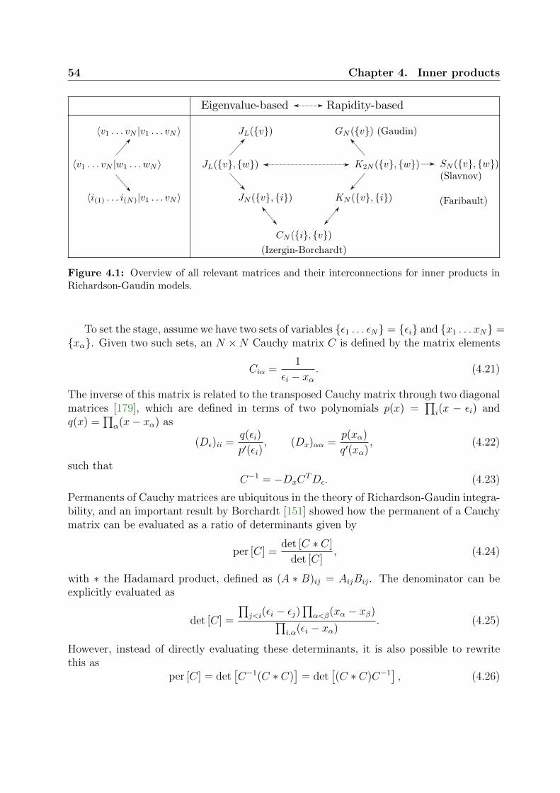
54 Chapter 4. Inner products
Figure 4.1: Overview of all relevant matrices and their interconnections for inner products inRichardson-Gaudin models.
To set the stage, assume we have two sets of variables ε1 . . . εN = εi and x1 . . . xN =xα. Given two such sets, an N ×N Cauchy matrix C is defined by the matrix elements
Ciα =1
εi − xα. (4.21)
The inverse of this matrix is related to the transposed Cauchy matrix through two diagonalmatrices [179], which are defined in terms of two polynomials p(x) =
∏i(x − εi) and
q(x) =∏
α(x− xα) as
(Dε)ii =q(εi)
p′(εi), (Dx)αα =
p(xα)
q′(xα), (4.22)
such thatC−1 = −DxC
TDε. (4.23)
Permanents of Cauchy matrices are ubiquitous in the theory of Richardson-Gaudin integra-bility, and an important result by Borchardt [151] showed how the permanent of a Cauchymatrix can be evaluated as a ratio of determinants given by
per [C] =det [C ∗ C]
det [C], (4.24)
with ∗ the Hadamard product, defined as (A ∗ B)ij = AijBij. The denominator can beexplicitly evaluated as
det [C] =
∏j<i(εi − εj)
∏α<β(xα − xβ)∏
i,α(εi − xα). (4.25)
However, instead of directly evaluating these determinants, it is also possible to rewritethis as
per [C] = det[C−1(C ∗ C)
]= det
[(C ∗ C)C−1
], (4.26)

4.2. Properties of Cauchy matrices 55
as noted in Ref. [156]. Because of the known structure of the inverse of a Cauchy matrix,these matrices can be explicitly calculated as
C−1(C ∗ C) = DxJxD−1x , (C ∗ C)C−1 = D−1
ε JεDε, (4.27)
with the J-matrices given by
(Jx)αβ =
−∑i
1xα−εi +
∑κ6=α
1xα−xκ if α = β,
− 1xα−xβ if α 6= β,
(4.28)
(Jε)ij =
∑α
1εi−xα −
∑k 6=i
1εi−εk if i = j,
− 1εi−εj if i 6= j,
(4.29)
and the D-matrices are those arising in the equation for the inverse (4.23). This nowpresents two different ways of evaluating the permanent as a determinant
per [C] = det [Jε] = det [Jx] . (4.30)
Because of the product structure of the J-matrices, an additional identity holds as
det [1N + Jx] = det[1N + C−1(C ∗ C)
]= det
[1N + (C ∗ C)C−1
]= det [1N + Jε] .
(4.31)Note that so far all involved matrices were N ×N matrices defined in terms of two sets ofvariables ε1 . . . εN and x1 . . . xN. Remarkably, this final expression (4.31) can immedi-ately be generalized towards matrices of different dimensions, defined in terms of sets witha different number of variables, playing an important role in connecting the inner productsto DWPFs. Given two such sets ε1 . . . εL and x1 . . . xN, with L 6= N , the following alsoholds
det [1N + Jx] = det [1L + Jε] , (4.32)
with Jx and N×N matrix and Jε an L×L matrix defined as in Eq. (4.28), but now in termsof sets with a different number of variables. This result can be obtained by generalizingEq. (4.31) towards non-square matrices and applying Sylvester’s determinant identity
det [1N + AB] = det [1L +BA] , (4.33)
with A an arbitrary N × L matrix and B an arbitrary L×N matrix.Returning to N ×N matrices, one final property of Cauchy matrices which will be key
in relating the eigenvalue-based determinant to Slavnov’s determinant, is that
2(C ∗ C)−1(C ∗ C ∗ C) = Dx
[Jx + CTJ−1
ε C]D−1x . (4.34)
This can be seen as a higher-order extension of the previous equality
C−1(C ∗ C) = DxJxD−1x , (4.35)
and leads to the determinant identity
det [2 (C ∗ C ∗ C)]
det [C ∗ C]= det
[Jx + CTJ−1
ε C]. (4.36)
56 Chapter 4. Inner products
4.3 From eigenvalue-based to Slavnov through dual
states
4.3.1 Dual states
The crucial element in all eigenvalue-based expressions is the (implicit) existence of dualstates for on-shell Bethe states. Any eigenstate of the RG integrable models can be con-structed in two different ways: either by creating excitations on top of a vacuum, or byannihilating excitations from a dual vacuum state [134, 154]. The former approach wasused so far, where eigenstates were constructed as
|v1 . . . vN〉 =N∏a=1
(L∑i=1
S+i
εi − va
)|↓ . . . ↓〉 , (4.37)
with rapidities v1 . . . vN satisfying the usual equations
1
g+
1
2
L∑i=1
1
εi − va−
N∑b 6=a
1
vb − va= 0, a = 1 . . . N. (4.38)
However, the latter approach states that eigenstates also have a dual representation givenby
|v′1 . . . v′L−N〉 =L−N∏a=1
(L∑i=1
S−iεi − v′a
)|↑ . . . ↑〉 , (4.39)
with the rapidities of this dual state satisfying
− 1
g+
1
2
L∑i=1
1
εi − v′a−
L−N∑b 6=a
1
v′b − v′a= 0, a = 1 . . . L−N. (4.40)
Note that these equations are related to the previous ones by changing the sign of g, whichcan be seen as a consequence of the spin-flip symmetry of the conserved charges (2.40).Because total spin-projection Sz =
∑Li=1 S
zi is a symmetry of the system, this also implies
that the same state will in general be described by a different number of rapidities in bothrepresentations.
Two such states are eigenstates of a given integrable Hamiltonian by construction, andthese can be made to represent the same eigenstate by demanding that their eigenvaluescoincide, leading to
N∑a=1
1
εi − va=
L−N∑a=1
1
εi − v′a− 2
g, i = 1 . . . L. (4.41)
While the correspondence between the rapidities of both representations is far from intu-itive, the correspondence between the eigenvalue-based variables is simple and given by
Λi(va) = Λi(v′a)−2
g, i = 1 . . . L. (4.42)

4.3. From eigenvalue-based to Slavnov through dual states 57
A special case is the g →∞ limit, where both sets of variables are equal up to a number ofdiverging rapidities going to infinity. In this limit, the conserved charges have an additionalsu(2) total spin symmetry, which is reflected in limv→∞ S+(v) ∼∑i S
+i , as also observed
in Ref. [180].These two different representations of a single eigenstate obviously have different nor-
malizations, but it is shown in Appendix 4.C that the ratio of these normalizations issimply given by
|v1 . . . vN〉 = (−1)N(g
2
)L−2N
|v′1 . . . v′L−N〉 . (4.43)
It is this ratio that is directly responsible for the appearance of the prefactor in Eq. (4.6),as will now be shown.
4.3.2 Inner products as DWPFs
Since the existence of dual states is guaranteed for on-shell Bethe states, it is alwayspossible to express inner products in terms of the dual state. The overlap between a(possibly off-shell) state |w1 . . . wN〉 and an on-shell state |v1 . . . vN〉 can now be written as
〈v1 . . . vN |w1 . . . wN〉 = (−1)N(g
2
)L−2N
〈v′1 . . . v′L−N |w1 . . . wN〉 . (4.44)
The overlap between a dual state and a normal state can be written out as
〈v′1 . . . v′L−N |w1 . . . wN〉 = 〈↑ . . . ↑|L−N∏a=1
(L∑i=1
S+i
εi − v′a
)N∏b=1
(L∑i=1
S+i
εi − wb
)|↓ . . . ↓〉 (4.45)
= 〈↑ . . . ↑|L∏α=1
(L∑i=1
S+i
εi − xα
)|↓ . . . ↓〉 , (4.46)
which can be interpreted as the overlap of a Bethe state defined by L rapidities xα =x1 . . . xL = v′ ∪ w with the dual vacuum |↑ . . . ↑〉,
〈↑ . . . ↑|L∏α=1
S+(xα) |↓ . . . ↓〉 =∑σ∈SL
L∏i=1
1
εi − xσ(i)
, (4.47)
which is known as a domain wall boundary partition function (DWPF), as introduced byKorepin [181]. This partition function also has a graphical interpretation, as illustrated inFigure 4.2.
For the models at hand and following Section 3.3, the expression (4.47) is exactly thedefinition of the permanent of a Cauchy matrix
〈↑ . . . ↑|L∏α=1
S+(xα) |↓ . . . ↓〉 = per [C] , (4.48)

58 Chapter 4. Inner products
(a) Vertices with non-zero weight. (b) Boundary conditions.
Figure 4.2: Graphical representation of the DWPF associated with the Bethe states. Thepartition function sums over all configurations of vertices in the bulk consistent with the boundaryconditions, with the total weight of each configuration given by the product of the weights of thevertices. The weights in the first column follow from 〈↑|S+(xα) |↓〉i.
with C the Cauchy matrix defined as
Ciα =1
εi − xα. (4.49)
Using the results on Cauchy matrices from the previous section (4.30), this permanent canbe rewritten as a determinant
per [C] = det [Jε] , (4.50)
with Jε an L× L matrix defined as
(Jε)ij =
∑Lα=1
1εi−xα −
∑Lk 6=i
1εi−εk if i = j,
− 1εi−εj if i 6= j.
(4.51)
Reintroducing the rapidities x1 . . . xL = v′ ∪ w in the diagonal elements leads to
(Jε)ij =
∑L−Na=1
1εi−v′a +
∑Nb=1
1εi−wb −
∑Lk 6=i
1εi−εk if i = j,
− 1εi−εj if i 6= j,
(4.52)
where, because of the correspondence between the eigenvalues of the original state and thedual state (4.41), this can be written entirely in terms of the original rapidities
(Jε)ij =
2g
+∑N
a=11
εi−va +∑N
b=11
εi−wb −∑L
k 6=i1
εi−εk if i = j,
− 1εi−εj if i 6= j,
(4.53)
resulting in the proposed determinant expression (4.6) for the inner product if the ratio ofnormalizations for the original state and the dual state (4.43) is taken into account. Note

4.3. From eigenvalue-based to Slavnov through dual states 59
that the existence of the dual state was necessary to derive these determinant expressions,but is only implicit in the final results due to the demand that one of the two states in theinner product must be on-shell.
At this point, the first proposed expression (4.6) has been derived, which is expressedin the eigenvalue-based variables. In order to derive the equivalent expression (4.8) for therapidities, the crucial observation is that the matrix (4.53) has the structure (1L+· · · ) aftermultiplying all matrix elements with g/2. This leads to the exact same structure obtainedwhen applying Sylvester’s determinant identity in Eq. (4.32). The involved matrices arenow defined in terms of two sets of variables of unequal size, being the L inhomogeneitiesε1 . . . εL and the 2N combined rapidities v1 . . . vN∪w1 . . . wN. Applying the relation(4.32) then connects the determinant of the L×L matrix (1L+ · · · ) to that of an 2N×2Nmatrix (12N + · · · ), equaling the matrix proposed in (4.8) after correcting for the missingprefactors of (g/2) in the matrix elements by changing the prefactor of the determinant.Afterwards, the related Gaudin and Izergin-Borchardt determinants follow immediately bytaking the appropriate limits.
4.3.3 Reduction to Slavnov’s determinant
Starting from the eigenvalue-based inner product (4.6), it is possible to rederive Slavnov’sdeterminant expression, obtaining other determinant expressions in the process and shed-ding some light on the structure of all involved identities.
First, by making using of the Bethe equations (4.10), the well-known Slavnov’s deter-minant expression (4.2) can be straightforwardly rewritten as
〈v1 . . . vN |w1 . . . wN〉 =
∏b
∏a(va − wb)∏
b<a(wb − wa)∏
a<b(vb − va)detSN(va, wb), (4.54)
SN(va, wb)ab =1
(va − wb)2
(L∑i=1
1
wb − εi− 2
N∑c 6=a
1
wb − vc− 2
g
). (4.55)
Note that, by rewriting the matrix elements in this way, the only explicit dependence on theinhomogeneities is through
∑i
1wb−εi , bringing to mind the eigenvalue-based determinants
and Eq. (4.8). The prefactor is the inverse of the determinant of the Cauchy matrix Udefined by
Uab =1
va − wb. (4.56)
Defining a diagonal N × N matrix Λ in order to absorb the dependency on the inhomo-geneities as
Λaa =L∑i=1
1
wa − εi− 2
N∑c=1
1
wa − vc− 2
g, (4.57)
the matrix in Slavnov’s determinant can be decomposed as
SN(va, wb) = (U ∗ U)Λ− 2(U ∗ U ∗ U). (4.58)

60 Chapter 4. Inner products
This can be summarized in
〈v1 . . . vN |w1 . . . wN〉 = det [U ]−1 det [(U ∗ U)Λ− 2(U ∗ U ∗ U)] . (4.59)
It is now possible to work towards this expression starting from the eigenvalue-basedexpressions using the presented properties of Cauchy matrices. The inner product as givenin Eq. (4.8) depends on a 2N × 2N matrix, which can be interpreted as a 2 × 2 blockmatrix of N ×N matrices as
〈v1 . . . vN |w1 . . . wN〉 = (−1)N detK2N(va, wb), (4.60)
with
K2N(va, wb) =
[Jv −UUT Jw − Λ
](4.61)
and the diagonal matrices are given by
(Jv)ab =
2g−∑L
i=11
va−εi +∑N
c 6=a1
va−vc +∑N
c=11
va−wc if a = b,
− 1va−vb if a 6= b,
(4.62)
(Jw)ab =
−∑N
c=11
wa−vc +∑N
c6=a1
wa−wc if a = b,
− 1wa−wb if a 6= b.
(4.63)
The dependence of Jw on the inhomogeneities can be absorbed in the same diagonal matrixΛ as defined for Slavnov’s determinant and the off-diagonal matrices are then determinedby the same Cauchy matrix (4.56) defined previously. Using the Bethe equations (4.10)for va in the diagonal elements of Jv then leads to
(Jv)ab =
−∑N
c 6=a1
va−vc +∑N
c=11
va−wc if a = b,
− 1va−vb if a 6= b.
(4.64)
By rewriting the matrix in this way, all submatrices exhibit the structures previouslyintroduced since Jv ∼ U−1(U ∗ U) and Jw ∼ (U ∗ U)U−1. One final step now consists ofrelating the determinant of a 2N × 2N matrix to that of an N × N one. For this, it ispossible to evaluate the determinant of a 2× 2 block matrix as
det
[A BC D
]= det (A) det
(D − CA−1B
). (4.65)
Applying this to the equation for the inner product yields
(−1)N det
[Jv −UUT Jw − Λ
]= (−1)N det(Jv) det(Jw − Λ + UTJ−1
v U)
= det(U)−1 det(U ∗ U) det[Λ− 2(U ∗ U)−1(U ∗ U ∗ U)
]= det(U)−1 det [(U ∗ U)Λ− 2(U ∗ U ∗ U)] , (4.66)

4.4. Extension to hyperbolic models 61
where det(Jv) = det(U ∗U)/ det(U) and Eq. (4.34) have been used to evaluate the inverseof Jv as
−Dw(Jw − Λ + UTJ−1v U)D−1
w = Λ− 2(U ∗ U)−1(U ∗ U ∗ U). (4.67)
This corresponds exactly to Slavnov’s determinant expression (4.54). Alternative ways ofcalculating the determinant of the block matrix would result in alternative N×N matrices,but their structure is more involved than that of the Slavnov determinant. Again, theon-shell requirement for one of the two states is crucial, arising here due to the impliedexistence of a dual state.
In conclusion, there are three ways of evaluating the inner product - by calculating thedeterminants of L× L, 2N × 2N , or N ×N matrices. The structure of all these matricesis intricately related to Cauchy matrices, where the 2N × 2N matrix can be reduced tothe N ×N Slavnov determinant, while the L×L matrix follows from the eigenvalue-basedframework. Similar results were also obtained in Refs. [180] and [182] for the rational six-vertex model, connecting DWPFs with Slavnov determinants, however without invokingthe dual representation of Bethe states. Alternatively, similar results were obtained byKitanine et al. for the integrable XXX Heisenberg chain through both a separation ofvariables and an ABA approach [183].
4.4 Extension to hyperbolic models
The presentation thus far was focused on the rational (XXX) Richardson-Gaudin models,because of their clear-cut connection with Cauchy matrices. However, it is possible toextend all results to the hyperbolic (XXZ) Richardson-Gaudin case, for which we will onlyprovide an overview and refer to Ref. [158] for a detailed derivation. Because of theirricher phase diagram and various symmetries, these expressions are slightly more involved.[72, 104–109]. This class is now defined by a similar set of commuting operators1 given by
Qi =
(Szi +
1
2
)+ g
L∑j 6=i
1
εi − εj
[√εiεj
(S+i S−j + S−i S
+j
)+ 2εi
(Szi S
zj −
1
4
)], (4.68)
and this section concerns the inner products of Bethe states
|v1 . . . vN〉 =N∏a=1
(L∑i=1
√εi
εi − vaS+i
)|↓ . . . ↓〉 . (4.69)
The normalizations of the original and the dual state are now related through (for L−2N >0)
|v′1 . . . v′L−N〉 = (−1)N∏N
a=1 va∏Li=1
√εi
[L−2N∏k=1
(g−1 + 1− k
)]|v1 . . . vN〉 . (4.70)
1We follow the presentation from Refs. [109, 184], which differs from the usual one in the asymmetry inthe last term. However, this allows for a clearer presentation and can be connected to the fact that thesemodels can also be constructed from a non-skew-symmetric r-matrix [106, 185, 186].

62 Chapter 4. Inner products
This is a more involved expression compared to the rational model (4.43), which can beseen as a consequence of the various symmetries and dualities present in this model – forspecific values g−1 ∈ Z the dual wave function vanishes because some of the dual rapiditiesdiverge [187]. Similar terms also arise in the investigation of the phase diagram of thesemodels [104, 107, 108].
From this, it is possible to obtain a similar set of determinant expressions for innerproducts in the hyperbolic model, leading to (for on-shell va)
〈v1 . . . vN |w1 . . . wN〉 = (−1)N
( ∏Li=1 εi∏Na=1 va
)[L−2N∏k=1
(g−1 + 1− k
)]−1
det JL(va, wb),
(4.71)with JL(va, wb) an L× L matrix given by
JL(va, wb)ij =
g−1
εi+∑N
a=11
εi−va +∑N
b=11
εi−wb −∑L
k 6=i1
εi−εk if i = j,
− 1εi−εj if i 6= j.
(4.72)
The diagonal elements of these matrices again reflect the structure of the eigenvalue-basedequations
εiΛi
(g−1
εi+ Λi
)−
L∑j 6=i
εiΛi − εjΛj
εi − εj= 0, Λi ≡ Λi(va) =
N∑a=1
1
εi − va, (4.73)
which can also be used to show the orthogonality of different eigenstates. When calculatingthe normalization of an on-shell state, this reduces to the Jacobian of the eigenvalue-basedequations (4.73), where all derivatives are now taken w.r.t. εiΛi instead of Λi. Alternatively,there is again a direct equivalence with the determinant of a 2N × 2N matrix defined interms of x1 . . . x2N = v1 . . . vN ∪ w1 . . . wN as
〈v1 . . . vN |w1 . . . wN〉 = (−1)N
(N∏b=1
wb
)detK2N(va, wb), (4.74)
with K2N(va, wb) a 2N × 2N matrix given by
K2N(va, wb)ab =
1+g−1
xa−∑L
i=11
xa−εi +∑2N
c6=a1
xa−xc if a = b,
− 1xa−xb if a 6= b,
(4.75)
where the diagonal elements now clearly reflect the Bethe equations
1 + g−1
va−
L∑i=1
1
va − εi+ 2
N∑c6=a
1
va − vc= 0, ∀a = 1 . . . N. (4.76)
The Slavnov determinant for the inner product of an on-shell and an off-shell state in theXXZ model [72] then follows from evaluating this matrix as a block matrix, where all steps

4.4. Extension to hyperbolic models 63
in the derivation are fundamentally the same as for the rational XXX model. The resultingexpression is given by
〈v1 . . . vN |w1 . . . wN〉 =
∏a
∏b(va − wb)∏
a<b(vb − va)∏
b<a(wb − wa)detSN(va, wb), (4.77)
with SN(va, wb) an N ×N matrix given by
SN(va, wb)ab =wb
(va − wb)2
(L∑i=1
1
wb − εi− 2
N∑c 6=a
1
wb − vc− g−1 + 1
wb
). (4.78)

Appendices
4.A Orthogonality of Bethe states
Starting from the determinant expressions of Eq. (4.5) or Eq. (4.8), the orthogonality ofdifferent Bethe states can easily be shown. Starting from two non-equal on-shell statesva and wb, it is straightforward to show that the rows of (4.6) are linearly dependentas
L∑i=1
[Λi(va)− Λi(wb)] JL(va, wb)ij
=
[Λj(va)2 +
2
gΛj(va)−
L∑i 6=j
Λj(va)− Λi(va)εj − εi
]
−[
Λj(wb)2 +2
gΛj(wb)−
L∑i 6=j
Λj(wb)− Λi(wb)εj − εi
]= 0, (4.79)
which vanish since these are exactly the eigenvalue-based equations satisfied by on-shellstates (4.7). The linear dependence of the rows implies that the determinant of this matrixalso vanishes, proving the orthogonality of different eigenstates
The orthogonality also follows from the similarity of the diagonal elements of (4.8)to the Bethe equations (4.10). Taking x1 . . . xN = v1 . . . vN and xN+1 . . . x2N =w1 . . . wN, this results in
N∑c=1
K2N(va, wb)cb −2N∑
c=N+1
K2N(va, wb)cb
=
2g
+∑L
i=11
εi−vb − 2∑N
c 6=b1
vc−vb = 0 if b = 1 . . . N,2g
+∑L
i=11
εi−wb − 2∑N
c 6=b1
wc−wb = 0 if b = N + 1 . . . 2N,(4.80)
64

4.B. From inner products to form factors 65
where we have identified wb and wN+b in the second line. Since these are exactly the Betheequations (4.10), the rows are again linearly dependent, leading to a vanishing determinantand orthogonal eigenstates.
4.B From inner products to form factors
The method of obtaining form factors starting from inner products will be illustrated onthe off-diagonal matrix elements 〈v1 . . . vN |Szk |w1 . . . wN〉 = 〈va|Szk |wb〉, where bothstates are assumed to be on-shell. The first step consists of writing this matrix elementas a summation over inner products, for which various determinant expressions have beenpresented. This can be done using the standard commutation relations, where the actionof Szk on |wb〉 can be found as
Szk |wb〉 = Szk
N∏b=1
S+(wb) |↓ . . . ↓〉
=N∑b=1
N∏c 6=b
S+(wc)
[Szk , S+(wb)] |↓ . . . ↓〉+
(N∏b=1
S+(wb)
)Szk |↓ . . . ↓〉 , (4.81)
which can be related to the Gaudin algebra elements as
[Szk , S+(wb)] =
S+k
εk − wb= lim
λ→εk
εk − λεk − wb
S+(λ). (4.82)
Taking the inner product with the on-shell state |va〉, this matrix element can be writtenas
〈va|Szk |wb〉 = limλ→εk
N∑b=1
εk − λεk − wb
〈v1 . . . vN |w1 . . . wb → λ . . . wN〉 −1
2〈va|wb〉 ,
(4.83)
leading to a summation of inner products between an on-shell state |v1 . . . vN〉 and a set ofoff-shell states |w1 . . . wb → λ . . . wN〉. Since the two states were assumed to be orthogonal,the term −1
2〈va|wb〉 generally vanishes, although this can easily be taken into account
otherwise.
4.B.1 Rapidity-based form factors
This can be rewritten as the determinant of a single matrix starting from Slavnov’s deter-minant expression. The matrix representation from Eq. (4.54) has the advantage that theonly dependence on the rapidity wb is in column b, so each term in the summation (4.83)

66 Chapter 4. Inner products
returns a matrix where only a single column b depends on λ. The limit λ → εk can beevaluated in this column, returning
limλ→εk
(εk − λ)SN(va, wb, wb → λ)ab = − 1
(va − εk)2. (4.84)
Defining this column as Q and denoting the separate columns of the matrix SN(va, wb)= (S1|S2| . . . |SN), this gives rise to
〈va|Szk |wb〉 = −N∑b=1
∏Na=1(va − εk)∏Na=1(wa − εk)
∏a,c6=b(va − wc)
∏c 6=b(wc − wb)∏
a<c(vc − va)∏
a>c(wc − wa)× det
(S1| . . . |Sb−1|Q|Sb+1| . . . |SN
). (4.85)
All dependence on the summation index b can be absorbed in the determinant by defining
(T )ab = SN(va, wb)ab ·N∏c=1
(vc − wb), Qab =1
(va − εk)2·N∏c 6=b
(wc − wb). (4.86)
Writing out both matrices as T = (T1|T2| . . . |TN) and Q = (Q1|Q2| . . . |QN) leads to
〈va|Szk |wb〉 =N∑b=1
∏Na=1(va − εk)∏Na=1(wa − εk)
det(T1| . . . |Tb−1|Qb|Tb+1| . . . |TN
)∏
a<c(vc − va)∏
a>c(wc − wa). (4.87)
The determinant is a multilinear function in its columns and the determinant of a matrixcontaining multiple linearly-dependent columns vanishes by definition, so this summationcan be seen as an expansion for the determinant of T+Q = (T1 +Q1|T2 +Q2| . . . |TN +QN).Expanding the determinant using the multilinearity in the columns, any term in the expan-sion containing multiple columns of Q will vanish because of their linear dependence. Thisonly leaves terms det(T1|T2| . . . |TN) = det(T ) = 0, also vanishing because of orthogonality,
and terms det(T1| . . . |Tb−1|Qb|Tb+1| . . . |TN
). The full expression then results in a single
determinant
〈va|Szk |wb〉 =
∏Na=1(va − εk)∏Na=1(wa − εk)
det[T + Q
]∏
a<c(vc − va)∏
a>c(wc − wa). (4.88)
4.B.2 Eigenvalue-based form factors
Alternatively, the eigenvalue-based framework returns
〈va|Szk |wb〉 =(−1)N(g
2
)L−2N
×(
[1 + Λk(wb)] det[JkL−1
]− det
[JkL−1 + F k
L−1
] ), (4.89)

4.B. From inner products to form factors 67
where two (L− 1)× (L− 1) matrices have been introduced. JkL−1 = JkL−1(va, wb) hasthe common structure of the J-matrices, but the row and column associated with the levelk are removed2 and εk has been excluded from the diagonal elements as
JkL−1(va, wb)ij =
2g
+ Λi(va) + Λi(wb)−∑L
l 6=i,k1
εi−εl if i = j,
− 1εi−εj if i 6= j,
(4.90)
and i, j 6= k. The second matrix F kL−1 = F k
L−1(wb) is a matrix where all rows are identicaland given by
F kL−1(wb)ij = −Λk(wb)− Λj(wb)
εk − εj, (4.91)
where again i, j 6= k. The proof of this determinant expression is surprisingly similar tothat of Eq. (4.88). From Eq. (4.83), it immediately follows that
〈va|Szk |wb〉 =N∑b=1
1
εk − wb〈v1 . . . vN |S+
k |w1 . . . wb−1wb+1 . . . wN〉
= (−1)N(g
2
)L−2NN∑b=1
1
εk − wbdet[JkL−1 −DL−1(wb)
], (4.92)
with JkL−1 defined as in Eq. (4.90) and DL−1(wb) an (L − 1) × (L − 1) diagonal matrixwith DL−1(wb)ii = 1
εi−wb. This diagonal matrix effectively removes the rapidity wb from
the summations in the diagonal elements of JkL−1.
The crucial step is to note that this equality remains valid if DL−1(wb) is extended froma diagonal matrix to a matrix with the same diagonal elements and matrix elements
DL−1(wb)ij =1
εj − wb, (4.93)
since this modifies the off-diagonal elements of(JkL−1 −DL−1(wb)
)as
(JkL−1 −DL−1(wb)
)ij
= − 1
εi − εj− 1
εj − wb= − 1
εi − εjεi − wbεj − wb
, (4.94)
corresponding to multiplying the row i by (εi − wb) and dividing column i by the samefactor, which leaves both the diagonal elements and the determinant invariant [188]. Theseparate rows of both matrices can now be written down as
JkL−1 = (J1|J2| . . . |JL−1)T , DL−1(wb) = (D(wb)|D(wb)| . . . |D(wb))T , (4.95)
2The indices i, j = 1 . . . k − 1, k + 1, . . . L now function as labels for 1 . . . L − 1 when denoting matrixelements of a (L− 1)× (L− 1) matrix.

68 Chapter 4. Inner products
where the determinant of JkL−1 −DL−1(wb) can be expanded as
det(JkL−1 −DL−1(wb)
)T= det (J1 −D(wb)|J2 −D(wb)| . . . |JL−1 −D(wb))
T
= det (J1|J2| . . . |JL−1)T −L−1∑i=1
det (J1| . . . |Ji−1|D(wb)|Ji+1| . . . |JL−1)T , (4.96)
since the determinant is a multilinear function in its rows and the determinant of a matrixcontaining multiple equal D-rows vanishes by definition. The first matrix returns exactlyJkL−1, while all other matrices reduce to JkL−1 where a single row i has been replaced bythe row D. Plugging this into Eq. (4.92) leads to
〈va|Szk |wb〉 ∝N∑b=1
1
εk − wbdet(JkL−1
)−
L−1∑i=1
N∑b=1
1
εk − wbdet (J1| . . . |Ji−1|D(wb)|Ji+1| . . . |JL−1)T , (4.97)
with the usual proportionality factor (−1)N (g/2)L−2N . Performing the summation overrapidities and absorbing the prefactor in the definition of the row F =
∑Nb=1
1εk−wb
D(wb),
the same arguments can be used to reduce the summation to
〈va|Szk |wb〉 ∝N∑b=1
1
εk − wbdet(JkL−1
)−
L∑i=1
det (J1| . . . |Ji−1|F |Ji+1| . . . |JL−1)
∝
1 +N∑b=1
1
εk − wb
det(JkL−1
)− det (J1 + F |J2 + F | . . . |JL−1 + F ) .
(4.98)
Defining F kL−1 as the matrix where all rows equal F , which can be evaluated as Eq. (4.91),
this returns the proposed expression (4.89). Alternatively, this can be obtained from thematrix determinant lemma [188].
4.C Normalizations of the normal and the dual state
From the identities presented in Section 4.2, it is possible to derive the ratio of the normal-izations of a dual Bethe state and a regular Bethe state. Since these are both eigenstateswith identical eigenvalues, they describe the same state but with different normalizations.It is now possible to calculate the ratio of the normalization of these states by taking theoverlap of both states with an (arbitrary) reference state, and to show how it leads to the

4.C. Normalizations of the normal and the dual state 69
proposed expression (4.43). To reiterate, a Bethe ansatz eigenstate for the Richardson-Gaudin models can be written in two representations as
|va〉 =N∏a=1
(L∑i=1
S+i
εi − va
)|↓ . . . ↓〉 , |v′a〉 =
L−N∏a=1
(L∑i=1
S−iεi − v′a
)|↑ . . . ↑〉 , (4.99)
with the (dual) rapidities satisfying the Richardson-Gaudin equations
1
g+
1
2
L∑i=1
1
εi − va−
N∑b 6=a
1
vb − va= 0, a = 1 . . . N, (4.100)
−1
g+
1
2
L∑i=1
1
εi − v′a−
L−N∑b 6=a
1
v′b − v′a= 0, a = 1 . . . L−N, (4.101)
describing the same eigenstate if these variables are coupled through
N∑a=1
1
εi − va+
2
g=
L−N∑a=1
1
εi − v′a, i = 1 . . . L. (4.102)
The crucial element in this proof is the existence of eigenvalue-based expressions for theinner product of a Bethe state and a reference state (see also Section 3.3). Defining areference state from a set of occupied levels can again be done in two ways
|iocc〉 =∏
i∈ioccS+i |↓ . . . ↓〉 =
∏i/∈iocc
S−i |↑ . . . ↑〉 , (4.103)
where both states are already normalized. Then the overlap of the original Bethe statewith this reference state is given by [154]
〈iocc|va〉 = det JN(va, iocc), (4.104)
with JN(va, iocc) an N ×N matrix defined as
JN(va, iocc)ij =
∑N
a=11
εi−va −∑
k∈iocck 6=i
1εi−εk if i = j,
− 1εi−εj if i 6= j,
i, j ∈ iocc. (4.105)
Alternatively, the overlap of the dual state with the same reference state can be written as
〈iocc|v′a〉 = 〈↓ . . . ↓|(L−N∏a=1
S−(v′a)
) ∏i/∈iocc
S+i
|↓ . . . ↓〉 . (4.106)
This final expression is the complex conjugate of the inner product of a regular Bethestate defined by the dual rapidities and a different reference state. Because all eigenvalue-based variables are real, these inner products are always real, and the same determinantexpressions can be invoked to write
〈iocc|v′a〉 = det JL−N(v′a, i|i /∈ iocc), (4.107)

70 Chapter 4. Inner products
with JL−N(v′a, i|i /∈ iocc) an (L−N)× (L−N) matrix defined as
JL−N(v′a, i|i /∈ iocc)ij =
∑L−N
a=11
εi−v′a −∑
k/∈iocck 6=i
1εi−εk if i = j,
− 1εi−εj if i 6= j,
i, j /∈ iocc.
(4.108)Because this only depends on the dual rapidities through the eigenvalue-based variables inthe diagonal elements, the correspondence (4.102) can be used to express this determinantin the rapidities of the original state as
〈iocc|v′a〉 = det
[2
g+ JL−N(va, i|i /∈ iocc)
]=
(2
g
)L−Ndet[1 +
g
2JL−N(va, i|i /∈ iocc)
]. (4.109)
Now Sylvester’s determinant identity can be used, as explained in Section 4.2, to exchangethe role of rapidities and inhomogeneities and obtain
〈iocc|v′a〉 =
(2
g
)L−Ndet[1 +
g
2KN(va, i|i /∈ iocc)
], (4.110)
with KN(va, i|i /∈ iocc) an N ×N matrix defined as
KN(va, i|i /∈ iocc)ab =
−∑i/∈iocc
1va−εi +
∑Nc6=a
1va−vc if a = b,
− 1va−vb if a 6= b.
(4.111)
Here, it is important to note the similarity between the diagonal elements of this matrix andthe Bethe equations (4.100). By slightly rewriting these equations, the diagonal elementscan be rewritten as
1− g
2
∑i/∈iocc
1
va − εi+g
2
N∑c 6=a
1
va − vc=g
2
∑i∈iocc
1
va − εi− g
2
N∑c 6=a
1
va − vc, (4.112)
resulting in
〈iocc|v′a〉 = (−1)N(
2
g
)L−2N
detKN(va, iocc). (4.113)
Both g/2 and the minus sign in the diagonal elements have been absorbed in a prefactor,since multiplying all rows with −1 and taking the transpose of the matrix returns theoriginal matrix but with the sign of the diagonal elements exchanged. The roles of bothvariables can again be exchanged in this final expression to obtain the original equality
〈iocc|v′a〉 = (−1)N(
2
g
)L−2N
〈iocc|va〉 . (4.114)
Since the set of reference states forms a complete basis and this equality holds for all suchstates, this yields the proposed expression (4.43) as
|v′a〉 = (−1)N(
2
g
)L−2N
|va〉 . (4.115)

CHAPTER 5
Integrability in the contraction limit of the quasispin
I like the speedAnd the incomparably blurredSensation of being deformedInto being and about to begin.
Frederick Seidel
So far, the Richardson-Gaudin models were formulated in terms of su(2)-algebras de-scribing spin states or fermion pairs, but these are far from exhaustive. The GGA con-struction does not depend explicitly on the su(2) realization, and various integrable modelsare known which contain e.g. a bosonic degree of freedom. Unfortunately, the direct con-nection between a solution to the Gaudin equations and the conserved charges and Betheansatz is somewhat muddled in these models. One possible way of retaining the clearstructure of the spin models is by starting from a spin model and introducing a bosonicdegree of freedom by means of a limiting procedure, deforming one of the spin degrees offreedom into a bosonic mode [34, 189, 190].
Two main classes of systems can be obtained in this way. Representative models forthese separate classes are the Dicke model [191–193], part of a family of Dicke-Jaynes-Cummings-Gaudin (DJCG) models describing two-level systems interacting with a singlephotonic mode of an electromagnetic field, and the two-channel extension of the px + ipymodel interacting through a p-wave Feshbach resonance [190]. Originally, the class ofDJCG models were obtained from the trigonometric RG model, which includes the Jaynes-Cummings [191], the Tavis-Cummings [192] and the inhomogeneous Dicke model [193],all describing the interaction between a (set of) two-level system(s) and a single bosonicelectromagnetic mode. The second class of systems considers the coupling of an integrablepx + ipy-wave superfluid to a bosonic mode, which can be obtained as the limiting case of
71

72 Chapter 5. Integrability in the contraction limit of the quasispin
a hyperbolic RG model [190]. This model was initially introduced by Dunning et al. [194]and can be shown to be equivalent to a model which couples Cooper pairs to condensedmolecular bosons [195]. These two classes were later obtained as two distinct cases ofintegrable Hamiltonians containing a bosonic degree of freedom, starting from a variationalapproach [196].
In this chapter, we show how these models can be constructed through a pseudo-deformation of the (quasi-)spin algebra [124], providing a controlled way of transformingthe hard-core bosonic su(2) algebra into a genuinely bosonic Heisenberg-Weyl algebrahw(1). The pseudo-deformation scheme was originally proposed as a way to shed lighton the singularities arising in the RG equations by connecting the spin models to purelybosonic models. However, here this method is used as a way to obtain a bosonic algebraas the contraction limit of a single su(2) quasispin algebra. The connection can be madeadiabatically by means of a continuous pseudo-deformation parameter, allowing for a sys-tematic extension of the su(2)-based integrable systems towards those containing a bosonicdegree of freedom [197].
This can also be used to find eigenvalue-based determinant expressions for overlaps inthese models. The dependency on the hw(1) algebra makes the generalization of results forthe su(2)-models towards models containing a bosonic degree of freedom far from straight-forward, because this algebra is non-compact and therefore lacks a highest weight state.Tschirhart and Faribault recently showed how determinant expressions could be found forthe form factors of the DJCG models by means of the introduction of an intricate alterna-tive Algebraic Bethe Ansatz (ABA) [155]. In this chapter, these expressions are obtainedas a limiting case of a renormalized pseudo-deformed spin model. The purpose of thischapter is twofold. It is shown how the pseudo-deformation scheme provides a convenientand relatively straightforward way of deriving all properties (eigenstates, eigenvalue-basedvariables, form factors, ...) of both the Dicke and extended px + ipy model, and how aneigenvalue-based framework can be obtained for the two classes of integrable RG modelscontaining a bosonic degree of freedom. This chapter is largely based on Refs. [197, 198].
5.1 Pseudo-deformation of the quasispin
There are multiple possible approaches for the process of bosonization, of which theHolstein-Primakoff transformation is arguably the best-known [199]. In this chapter, therecently-proposed pseudo-deformation scheme [124] is presented as a similar way of ob-taining bosonic commutation relations. This then provides an adiabatic, and thereforecontrolled, mapping from su(2) to hw(1). A pseudo-deformed algebra can be defined as
[Sz(ξ), S+(ξ)] = S+(ξ), [Sz(ξ), S−(ξ)] = −S−(ξ),
[S+(ξ), S−(ξ)] = 2 (ξSz(ξ) + (ξ − 1)s) (5.1)
with ξ ∈ [0, 1] the pseudo-deformation parameter and s the original (ξ = 1) su(2) irreplabel. This definition can be interpreted as providing a linear interpolation between twoknown limits: ξ = 1 gives rise to the original su(2) quasispin algebra, while ξ = 0 results in
5.1. Pseudo-deformation of the quasispin 73
a (unnormalized) bosonic hw(1) algebra. This latter limit was also termed the contractionlimit of the algebra [200]. The nomenclature pseudo-deformation was originally proposedbecause this algebra can be reduced to a canonical su(2)ξ algebra
[Az(ξ), A+(ξ)] = A+(ξ), [Az(ξ), A−(ξ)] = −A−(ξ),
[A+(ξ), A−(ξ)] = 2Az(ξ), (5.2)
by defining
A+(ξ) =1√ξS+(ξ), A−(ξ) =
1√ξS−(ξ), Az(ξ) = Sz(ξ) +
(1− 1
ξ
)s. (5.3)
This holds for all values of ξ except for the contraction limit ξ = 0. In this limit, thefollowing operators
b† =
√1
2sS+(0), b =
√1
2sS−(0), b†b = Sz(0) + s, (5.4)
close the bosonic hw(1) algebra
[b†b, b†] = b†, [b†b, b] = −b, [b, b†] = 1. (5.5)
The irreps of the A+(ξ), A−(ξ), Az(ξ) algebra are labeled by s(ξ) ≡ s/ξ. The interpre-tation behind this is a gradual increase of the effective multiplicity Ω(ξ) = (2s(ξ) + 1) ofthe su(2) irrep with decreasing ξ, in the contraction limit leading to an effective unlimitedoccupation consistent with the bosonic character. This is illustrated in Figure 5.1. Itshould be noted that only discrete values of ξn = 2s
n(with n = 2s, 2s + 1, . . . ) give rise to
unitary irreps. Nevertheless, this is not problematic because the theory of RG integrabilityis only based on commutation relations, so the parameter ξ can be regarded as a continuousvariable.
Recently, it has been shown how the Bethe ansatz states in the RG solution [28, 29]of the reduced BCS Hamiltonian for conventional superconductivity [15, 16] can be con-nected adiabatically to a product state of generalized bosons [124] employing a pseudodeformation of the quasispin algebra. The product structure of the Bethe ansatz stateis reminiscent of the projected BCS approximation, in which the superconducting stateis approximated by a condensate of collective Cooper pairs [14–16]. However, in gen-eral the rapidities parametrizing the generalized quasispin creation operators in the Betheansatz state differ from each other, which is not reconcilable with the concept of a truecondensate. The pseudo deformation can then be used to continuously deform the su(2)quasispin algebra of the BCS pairing Hamiltonian into a genuinely bosonic hw(1). Thereduced BCS Hamiltonian remains integrable along the path of deformation, allowing foran adiabatic and injective mapping of the exact Bethe ansatz states into a true conden-sate of (orthogonal) bosonic modes [201]. Accordingly, the coupled set of RG equations ofintegrability reduce to a single decoupled equation, equivalent to the secular equation ofthe particle-particle Tamm-Dancoff Approximation (pp-TDA) for the elementary pairing

74 Chapter 5. Integrability in the contraction limit of the quasispin
−6 −4 −2 0 2 4 6
m(ξ)
0.0
0.2
0.4
0.6
0.8
1.0
ξ
k = 0
k = 1
k = 2· · ·
∞ →← −∞ ......
......
.........
→← A+(ξ)
A−(ξ)
Figure 5.1: An illustration of the pseudo-deformed quasispin irreps |s(ξ),m(ξ)〉 of su(2)ξ. Theunitary irreps, at ξ = 2s
2s+k with k ∈ N, are denoted by open circles, connected by dashed lines.The lines connecting the lowest and highest weights with m(ξ) = ∓s(ξ) are drawn in full. Forξ = 1, the s(1) = 1 irrep is retained. Based on a similar figure in Ref. [124].
modes for the reduced BCS Hamiltonian [202]. Reversely, the pseudo deformation enablesone to numerically reconstruct the solution of the coupled set of non-linear RG equationsfrom the simpler decoupled secular pp-TDA equation, by adiabatically reintroducing thePauli principle in the integrable model [108, 124].
5.2 The Dicke model
The interaction of a single quantized mode of electromagnetic radiation (photons) with atwo-state system, such as a nuclear spin or two-level atom, can be modeled by means ofthe Rabi Hamiltonian [203]. Although simple and physically transparent in its formula-tion, the structure of the eigenstates of the Rabi Hamiltonian are quite involved due tothe ‘counter-rotating’ interaction terms in the Hamiltonian [204]. In the resonance regimehowever, these fast-frequency counter-rotating terms average out with respect to the col-lective two-level oscillations, and can be neglected in first-order perturbation theory (theso-called Rotating Wave Approximation (RWA)). This gives rise to the Jaynes-Cummings(JC) Hamiltonian of quantum electrodynamics [191]. Due to the RWA, the JC Hamilto-nian exhibits an additional symmetry, which allows for the decomposition of the Hilbertspace into irreps conserving the total number of (bosonic and atomic) excitations. Forthe two-level (s = 1/2 quasispin) formulation of the JC model, these irreps remain two-dimensional and therefore reduce to two-level mixing models. One of the successes of the-

5.2. The Dicke model 75
oretical and experimental quantum mechanics is that such simple theoretical models havebeen validated in sophisticated experiments situated in cavity quantum electrodynamics[205], circuit quantum electrodynamics [206],...
A direct consequence of the additional symmetry is that the two-level JC model ex-hibits two linearly independent conserved operators, i.e. the Hamiltonian and the operatorcounting the total number of excitations. As the model has two degrees of freedom (theelectromagnetic photon mode and the two-level system), the model is integrable by def-inition, and supports a Bethe ansatz wave function [35]. This result can be extended togeneral (2s+1)-level systems, also referred to as Tavis-Cummings models [192], or a collec-tion of inequivalent (2s+ 1)-level systems interacting via a single mediating bosonic mode,called the Dicke model [193]. The integrability of the Dicke model was first established byGaudin [35], by means of an infinite-dimensional Schwinger representation of the centralspin in the Gaudin magnet. Later, the full set of conserved charges of the Dicke modelwas derived by Dukelsky et al. [189] by mapping one of the su(2) quasispin copies of theRichardson-Gaudin conserved charges onto the bosonic mode. As an integrable model, theconserved charges and Bethe ansatz state of the Dicke model can also be obtained fromthe ABA [138], however a direct and simplified derivation of the Bethe ansatz state withthe corresponding Bethe equations solution is feasible using a commutator scheme [207].
The Dicke Hamiltonian [193] is given by
H = ε0b†b+
L∑i=1
εiSzi +G
L∑i=1
(S+i b+ S−i b
†) , (5.6)
and describes a set of L (2si+1)-level systems with energy differences εi interacting with asingle mode of the bosonic field, represented by a photon with energy ε0. The interactionstrength is tunable through the single coupling constant G.
This Hamiltonian can now be related to the models from Chapter 2 through the pseudo-deformation scheme. Starting from the constants of motion for a set of L + 1 interactingspins (2.40), these are labeled i = 0, 1, . . . , L, and the su(2) algebra labeled i = 0 isreplaced by a pseudo-deformed su(2)ξ algebra. The trigonometric Gaudin algebra (2.16)can be mapped to
X(ηi, ηj) =
√(1 + η2
i )(1 + η2j )
ηi − ηj, Z(ηi, ηj) =
1 + ηiηjηi − ηj
, (5.7)
and taking the limit η0 →∞ leads to a Gaudin algebra determined by (for i, j 6= 0)
X(η0, ηj) =√
1 + η2j , Z(η0, ηj) = ηj, (5.8)
X(ηi, ηj) =
√(1 + η2
i )(1 + η2j )
ηi − ηj, Z(ηi, ηj) =
1 + ηiηjηi − ηj
. (5.9)

76 Chapter 5. Integrability in the contraction limit of the quasispin
The conserved charge associated with the deformed algebra is given by
Q0(ξ) = Az(ξ) + gL∑j=1
[1
2X(η0, ηj)
(A+(ξ)S−j + A(ξ)−S+
j
)+ Z(η0, ηj)A
z(ξ)Szj
]
= Az(ξ) + g
L∑j=1
[1
2
√1 + η2
j
(A+(ξ)S−j + A−(ξ)S+
j
)+ ηjA
z(ξ)Szj
]. (5.10)
It is now possible to define a ξ-dependent coupling constant as g =√
2ξs0G2
G2
ε0and rescale
the variables ηj = −√
ξ2s0G2 εj. Near the contraction limit (ξ 1) the Gaudin algebra
reduces to
X(η0, ηj) = 1 +ξ
4s0G2ε2j +O(ξ2), Z(η0, ηj) = −
√ξ
2s0G2εj, (5.11)
which is related to the parametrization proposed by Dukelsky et al. [189]. By makinguse of this parametrization, the Dicke Hamiltonian can be obtained (up to a divergingconstant) in the contraction limit as
ε0Q0(ξ → 0) = ε0b†b+
L∑i=1
εiSzi +G
L∑i=1
(S+i b+ S−i b
†) , (5.12)
A similar procedure leads to the other properties of the Dicke model.
1. The constants of motion
ε0Qi(ξ → 0) =(ε0 − εi)Szi −G(S+i b+ S−i b
†)
− 2G2
L∑j 6=i
1
εi − εj
[1
2(S+
i S−j + S−i S
+j ) + Szi S
zj
]. (5.13)
2. The underlying GGA, where the rescaling of the inhomogeneities results in a rationalGGA instead of the original trigonometric one,
S+(u) = b† +GL∑i=1
S+i
u− εi, S−(u) = b+G
L∑i=1
S−iu− εi
,
Sz(u) =ε0 − u
2G−G
L∑i=1
Sziu− εi
. (5.14)
3. The Bethe ansatz for the Dicke model
|v1 . . . vN〉 =
(2s0
ξ
)N2
N∏a=1
(b† −G
L∑i=1
S+i
εi − va
)|0〉 , (5.15)
where the prefactor can be absorbed in the normalization and the vacuum state isgiven by |0〉 = |0〉 ⊗ |s1,−s1〉 ⊗ · · · ⊗ |sL,−sL〉.

5.3. The extended px + ipy-wave pairing model 77
4. The Bethe equations
(ε0 − va)− 2G2
L∑i=1
siεi − va
+ 2G2
N∑b 6=a
1
vb − va= 0, ∀a = 1 . . . N. (5.16)
Remarkably, it remains possible to transform the equations for the rapidities to an equiv-alent set of equations for the set of eigenvalue-based variables provided si = 1/2,∀i =1, . . . , L [136, 138]. For the Dicke model, the relevant variables are given by
Λ0 =N∑a=1
va, Λi ≡ Λi(va) =N∑a=1
1
εi − va, i = 1 . . . L, (5.17)
and these determine the eigenvalues of the constants of motion (5.13) as
ε0Qi |v1 . . . vN〉 =1
2
[(εi − ε0) + 2G2
N∑a=1
1
εi − va−G2
L∑j 6=i
1
εi − εj
]|v1 . . . vN〉 ,
while satisfying the coupled quadratic equations
G2Λ2i = N − Λi(εi − ε0) +G2
L∑j 6=i
Λi − Λj
εi − εj, ∀i = 1 . . . L,
Λ0 +G2
L∑i=1
Λi = ε0N. (5.18)
These equations can either be determined starting from the Bethe equations for the Dickemodel [136, 138, 155], or by taking the contraction limit of the eigenvalue-based equationsfor the trigonometric RG model. Similar to the su(2)-based RG models, it is possible toexpress the overlap and form factors of the Dicke model in the eigenvalue-based variablesonly, again circumventing the need to calculate the singularity-prone rapidities [155] (seeSection 5.4).
5.3 The extended px + ipy-wave pairing model
A similar procedure can be used to prove the integrability of the px + ipy-wave pairingmodel coupled to a bosonic degree of freedom. This model was introduced by Dunning etal. [194] as an extension of the integrable fermionic px + ipy-pairing model [72, 104, 107].Lerma et al. consequently showed how this model is given by the limit of a hyperbolic RGmodel [190], which here will be reformulated by making use of the pseudo-deformation.The Hamiltonian is given by
H =δ b†b+∑k
k2
2mc†kck −
G
4
∑k 6=±k′
(kx − iky)(k′x + ik′y)c†kc†−kck′c−k′
− K
2
∑k
((kx − iky)c†kc†−kb+ h.c.
), (5.19)

78 Chapter 5. Integrability in the contraction limit of the quasispin
and was shown to be integrable if
δ = −F 2G, K = FG. (5.20)
By making use of the quasispin formalism [94] and again absorbing a phase in the quasispinoperators, the Hamiltonian can be rewritten as
H = δ b†b+L∑k=1
εkSzk −G
L∑k,k′=1
√εkε′kS
+k S−k′ −K
L∑k=1
√εk(S+k b+ S−k b
†) , (5.21)
which can again be related to a su(2)-based RG model. This suggests starting from thehyperbolic Gaudin algebra (2.15),
X(εi, εj) = 2
√εiεj
εi − εj, Z(εi, εj) =
εi + εjεi − εj
. (5.22)
Taking the conserved charges for (L+1) levels and exchanging a single su(2) algebra with apseudo-deformed su(2)ξ-algebra, the Hamiltonian can be obtained as a linear combinationof the conserved charges in the contraction limit. Renormalizing the coupling constant andbosonic energy level ε0 as
g =ξ
s0 + ξκ, ε0 =
ξ
2s0
η20, (5.23)
the conserved charges reduce to
limξ→0
Q0(ξ) = b†b+L∑i=1
Szi ≡ N, (5.24)
limξ→0
s0
ξQi(ξ) =
L∑j 6=i
[ √εiεj
εi − εj(S+i S−j + S−i S
+j
)+εi + εjεi − εj
Szi Szj
]+
η0√εi
(S+i b+ S−i b
†)+ Szi
(κ+ b†b− η2
0
εi
), (5.25)
with N the number operator counting the number of excitations. Note that Qi(ξ →0) = 0, but Qi(ξ)/ξ remains finite for the whole range of ξ and results in a non-zeroconserved operator in the contraction limit. These operators are the building blocks forthe Hamiltonian (5.21), similar to the results presented for the fermionic px + ipy pairingmodel [107]. The integrability condition (5.20) arises naturally from the parametrizationof the Gaudin algebra. The related Hamiltonian studied in Ref. [195] can be obtained bytaking the linear combination
H =L∑i=1
Qi =L∑i=1
η0√εi
(S+i b+ S−i b
†)− L∑i=1
η20
εiSzi +
L∑i=1
Szi (b†b+ κ), (5.26)
which also equals the two-channel px + ipy-wave superfluid Hamiltonian introduced byLerma et al. [190] up to a rescaling, a redefinition of the energy levels as 1/εi, and byexpressing
∑Li=1 S
zi = N − b†b. All other properties of these models can similarly be
obtained from the contraction limit.

5.4. Eigenvalue-based determinant expressions 79
1. The underlying GGA remains the hyperbolic model, with generators given by
S+(u) = 2η0√ub† + 2
L∑i=1
√uεi
u− εiS+i , S−(u) = 2
η0√ub+ 2
L∑i=1
√uεi
u− εiS−i ,
Sz(u) =η2
0
u− b†b− κ
L∑i=1
u+ εiu− εi
Szi . (5.27)
2. The Bethe states for these models can similarly be found from the contraction limitas
|v1 . . . vN〉 =N∏a=1
(b† −
L∑i=1
√εiva
εi − vaS+i
η0
)|0〉 . (5.28)
3. The resulting Bethe equations are now given by
κ− η20
va+
L∑i=1
siεi + vaεi − va
−N∑b6=a
vb + vavb − va
= 0, ∀a = 1 . . . N. (5.29)
Taking again si = 1/2, ∀i = 1 . . . L, these now result in a set of quadratic equations in thevariables
Λ0 =N∑a=1
η20
va, Λi =
N∑a=1
εi + vaεi − va
, ∀i = 1 . . . L, (5.30)
which have to satisfy
Λ2i = −N(L−N)− 2κΛi + 2η2
0
(Λ0 +
Λi + L
εi
)+
L∑j 6=i
εi + εjεi − εj
(Λi − Λj), ∀i = 1 . . . L,
2Λ0 =L∑i=1
Λi + 2κL. (5.31)
These again fully determine the eigenvalues of the conserved charges as
Qi |v1 . . . vN〉 =1
2
[−κ−
N∑a=1
εi + vaεi − va
+η2
0
εi+
L∑j 6=i
εi + εjεi − εj
]|v1 . . . vN〉 . (5.32)
5.4 Eigenvalue-based determinant expressions
In the previous section, it was shown how many results for integrable systems containing abosonic degree of freedom can be obtained in the contraction limit. However, when derivingexpressions for normalizations and form factors starting from the su(2) spin models, we

80 Chapter 5. Integrability in the contraction limit of the quasispin
face the problem that the bosonic level has no state of maximum occupation number.A dual vacuum now cannot be defined since this would contain an infinite number ofbosonic excitations. This problem was first envisioned for the Dicke model by Tschirhartand Faribault [155], who devised an alternative formulation of the ABA, introducing apseudovacuum, which allowed for a description in terms of the eigenvalue-based variablesfor the Dicke model. The pseudo-deformation scheme now allows for a simpler derivation ofthese results by means of a renormalization procedure. Starting from the eigenvalue-baseddeterminant expressions for the XXZ RG models, the dual state can still be defined for anyBethe ansatz eigenstate. Determinant expressions can then be obtained while keeping thedual state implicit, leading to finite expressions in the contraction limit. This approachcan then be extended to the px+ ipy-wave pairing model. In a similar manner as presentedin the previous chapter, it can be expected that these results can be recast using theunderlying Cauchy matrix structure to return the Slavnov determinant [208].
A determinant expression for the overlap of an arbitrary Bethe ansatz state in theDicke model with an uncorrelated product state will first be derived. The expressions forthese overlaps do not depend on the existence of a dual state, nor a dual vacuum state,so the inclusion of a bosonic level into the existing fermionic su(2) models in the pseudo-deformation is well defined. The main difference with the previously-considered spin-1/2models is the occurrence of the bosonic level with arbitrary occupation number. Theexpansion with permanents as expansion coefficients still holds, but since multiple columnsof the permanent can be equal, these can not immediately be rewritten as determinants.This problem can be avoided by introducing a limiting procedure. The permanent of acoefficient matrix with distinct columns can be rewritten as a determinant, so we willintroduce a matrix with different columns and consider the limit where multiple columnsbecome equal. The overlaps can then be found by a two-step limiting procedure: first thepermanent with multiple equal columns can be reduced to a determinant, after which thecontraction limit can be taken. The expressions for inner products can be derived in asimilar way with only minor modifications, as shown in Ref. [198].
Assume a model where all spins si = 1/2, except for one level (again labeled 0) with anarbitrary large degeneracy. The Bethe state can then be expanded in a set of basis statesas
N∏a=1
(X(η0, µa)S
+0 +
L∑i=1
X(ηi, µa)S+i
)|0〉
=∑
[i(a)]φ[i(a)]N0!
(S+
0
)N0
(N−N0∏a=1
S+i(a)
)|0〉 , (5.33)
with the summation running over all subsets [i(a)] = [i(1) . . . i(M)] of the set [1, 2 . . . L]

5.4. Eigenvalue-based determinant expressions 81
containing M = N −N0 elements. The expansion coefficients can now be written down as
φ[i(a)] = per
X(η0, µ1) . . . X(η0, µ1) X(ηi(1), µ1) . . . X(ηi(M), µ1)X(η0, µ2) . . . X(η0, µ2) X(ηi(1), µ2) . . . X(ηi(M), µ2)
......
......
︸ ︷︷ ︸N0
X(η0, µN) . . . X(η0, µN) X(ηi(1), µN) . . . X(ηi(M), µN)
. (5.34)
In the following, it will be shown how this permanent can be written as the determinantof an M ×M -matrix for the trigonometric realization of the Gaudin algebra leading to theDicke model. The Gaudin algebra elements (5.11) associated with the bosonic level aregiven by
X(η0, µa) =√
1 + µ2a = lim
η0→∞
√(1 + η2
0)(1 + µ2a)
η0 − µa. (5.35)
Instead of immediately taking the limit η0 → ∞, it is possible to first evaluate the per-manent for arbitrary η0 and later take this limit. Instead of using the same parameter η0
for each column and taking the limit for each column simultaneously, it is also possible tointroduce a different variable λi (replacing η0) for each column i, and taking consecutivelimits to infinity of these parameters. This reduces the problem to the evaluation of
limλ1,...λN0
→∞per
X(λ1, µ1) . . . X(λN0 , µ1) X(ηi(1), µ1) . . . X(ηi(M), µ1)X(λ1, µ2) . . . X(λN0 , µ2) X(ηi(1), µ2) . . . X(ηi(M), µ2)
......
......
︸ ︷︷ ︸N0
X(λ1, µN) . . . X(λN0 , µN) X(ηi(1), vN) . . . X(ηi(M), µN)
.
(5.36)
This is the permanent of a matrix where each matrix element satisfies the Gaudin algebra(2.16), for which a determinant representation can be obtained using the results fromSection 3.3. Extending this set of variables as λ1 . . . λN = λ1 . . . λN0 ∪ ηi(1) . . . ηi(M)
φ[i(a)] = limλ1→∞
. . . limλN0→∞
∏Na=1
√1 + µ2
a∏Na=1
√1 + λ2
a
det JN , (5.37)
with JN defined as
(JN)ab =
λa +
∑Nc=1
1+λaµcλa−µc −
∑Nc6=a
1+λaλcλa−λc if a = b,√
1+λ2a√
1+λ2bλa−λb if a 6= b.
(5.38)
This is simply the application of Eq. (3.40) with the gauge u tending to infinity. Absorbingthe factors (1 + λ2
a)1/4 ≈
√λa, a = 1 . . . N0, from the prefactor into the first N0 columns i
82 Chapter 5. Integrability in the contraction limit of the quasispin
and the first N0 rows i and taking the subsequent limits to infinity as λ1 λ2 · · · λN0 ,the overlap returns
φ[i(a)] =
∏Na=1
√1 + µ2
a∏Ma=1
√1 + η2
i(a)
det
1 . . . 0 0...
...0 . . . N0 00 . . . JM
= N0!
∏Ma=1
√1 + µ2
a∏Ma=1
√1 + η2
i(a)
det[JM ],
(5.39)
with the M ×M matrix JM defined as
(JM)ab =
(N0 + 1)ηi(a) +∑N
c=1
1+ηi(a)µc
ηi(a)−µc −∑N
c 6=a1+ηi(a)ηi(c)ηi(a)−ηi(c) if a = b,√
1+η2i(a)
√1+η2
i(b)
ηi(a)−ηi(b) if a 6= b.(5.40)
The contraction limit can now be taken without any problems, leading to the overlap
between a basis state |N0; i(a)〉 =(b†)N0∏M
a=1 S+i(a) |0〉 and a Bethe state in the Dicke
model as〈N0; i(a)|v1 . . . vN〉 =
√N0!(−G)M det JM , (5.41)
with JM exhibiting the usual structure of
(JM)ab =
∑Nc=1
1εi(a)−vc −
∑Mc 6=a
1εi(a)−εi(c) if a = b,
1εi(a)−εi(b) if a 6= b.
(5.42)
A similar procedure can be used to obtain determinant expressions for the overlaps betweenoriginal states and dual states, for which this final expression provides the building block.Repeating this for the extended px + ipy model then returns an expansion of the Bethestate
|v1 . . . vN〉 =N∏a=1
(b† −
L∑i=1
√εiva
εi − vaS+i
η0
)|0〉 , (5.43)
with expansion coefficients
〈N0; i(a)|v1 . . . vN〉 =
√N0!√∏a εi(a)
det JMηM0
, (5.44)
where JM is now defined as
(JM)ab =
12
∑Nc=1
εi(a)+vc
εi(a)−vc −∑M
c 6=a12
εi(a)+εi(c)εi(a)−εi(c) −
N0+12
if a = b,√εi(a)εi(b)
εi(a)−εi(b) if a 6= b.(5.45)
These results can be extended towards normalizations and inner products by following thesame route. Here, the results for XXZ models with spin-1/2 containing a single spin witharbitrary degeneracy can be immediately extended towards models with a bosonic degreeof freedom. While no dual state exists in the contraction limit, a dual state can be foundfor the XXZ models at arbitrary degeneracies and determinant expressions can again beobtained in which the dual state is implicit. These will not be repeated due to the largelysimilar derivation, but can be found in Ref. [198].

Part II
Applications
83


CHAPTER 6
Read-Green resonances in a topological superconductor
coupled to a bath
Topology is the property of something that doesn’t changewhen you bend it or stretch it as long as you don’t breakanything.
Edward Witten
The coming chapters now involve applications of the framework presented in the firsthalf of this thesis to various physical domains. In this chapter, a topological px+ ipy super-conductor capable of exchanging particles with an environment is studied. This additionalinteraction breaks particle-number symmetry, but can still be modeled by means of anintegrable Hamiltonian building on the class of XXZ Richardson-Gaudin pairing models.The isolated system supports zero-energy modes at a topological phase transition, whichdisappear when allowing for particle exchange with an environment. However, it is shownfrom the exact solution that these still play an important role in system-environment par-ticle exchange, which can be observed through resonances in low-energy and -momentumlevel occupations. These fluctuations signal topologically protected Read-Green points andcannot be observed within traditional mean-field theory.
The first successful description of superconductivity was given by Bardeen, Cooper, andSchrieffer (BCS) by introducing a collective ground state consisting of condensed Cooperpairs, explicitly violating conservation of particle number [16]. This original mean-field the-ory was formulated for an s-wave pairing interaction, where the gap function is assumedisotropic. As mentioned in Section 2.7.3, it was later shown how topological superconduc-tivity arose from a chiral px + ipy-wave interaction by breaking time-reversal symmetry[110, 111]. Most of the theoretical insights into topological superconductivity are basedon mean-field Bogoliubov-de Gennes theory, as initiated by Read and Green [110]. One
85

86 Chapter 6. Read-Green resonances
of their crucial results was the uncovering of a phase transition between a (topologicallynontrivial) weak-pairing and a (topologically trivial) strong-pairing state. At this transi-tion, the chemical potential vanishes and the Bogoliubov quasiparticle spectrum becomesgapless. The main goal is now to put the robustness of the topological phase transition ina finite system to test when exchange of particles with an environment is allowed. For this,a px + ipy superconductor coupled to a bath system is modeled by means of a recently-proposed integrable model [184]. The Hamiltonian can be regarded as a hybrid between anintegrable number-conserving Hamiltonian describing superconductivity and a mean-fieldterm coupling this system to an infinite bath, allowing for particle-number fluctuations.
First, the topological nature of the isolated system is discussed both from the mean-fieldand the Bethe ansatz wave function, after which the integrable Hamiltonian is extendedby coupling it to a bath. The exact Bethe eigenstates are presented together with theBethe and eigenvalue-based equations. As can be expected from a particle-number non-conserving Hamiltonian, the exact eigenstates mix separate U(1)-gauge (particle-number)symmetry sectors. Interestingly, they retain the common factorized form of Bethe states.This exact solution is found to be essential to observe the effects of particle-exchange on thetopological phase transition. It is shown how zero-energy excitations associated with thephase transition govern the particle-exchange with the bath, resulting in avoided crossingsbetween states from different U(1)-symmetry sectors at the Read-Green points. These canbe observed from strong fluctuations in the single-particle level occupations. This connectsthe physics of zero-energy excitations, arising from topological phase transitions, with thephysics of open quantum systems. Furthermore, it is shown that while the breaking ofparticle-number symmetry in mean-field Bogoliubov-de Gennes theory has known greatsuccess in the description of number-conserving superconductors, it fails in describing thefluctuations observed in the exact solution. The goal of this chapter is then twofold: toshow how Bethe states can still be obtained even if particle-number U(1) symmetry isbroken and to investigate the physical effects of particle-exchange. The present chapter islargely based on Ref. [209].
6.1 Topological superconductivity
6.1.1 Mean-field theory
The px + ipy pairing Hamiltonian as introduced in Chapter 2 is given by
Hp+ip =∑k
|k|22m
c†kck −G
4m
∑k,k′
k 6=±k′
(kx + iky)(k′x − ik′y)c†kc†−kc−k′ck′ , (6.1)
in which ck and c†k denote annihilation and creation operators respectively for spinlessfermions of mass m with two-dimensional momentum k = (kx, ky), and a dimensionlesscoupling constantG has been introduced (2.59). Within mean-field theory, the Hamiltonian

6.1. Topological superconductivity 87
(6.1) can be approximated by the quadratic Hamiltonian
Hmf =∑k
ε(k)c†kck −[
∆
2
∑k
(kx + iky)c†kc†−k + h.c.
]+
2m
G|∆|2 + µN, (6.2)
where a BCS pairing gap/order parameter ∆ and mean-field single-particle energies havebeen defined as
∆ =G
2m
∑k
(kx − iky) 〈c−kck〉 , ε(k) = (1 +G)|k|22m− µ. (6.3)
The interaction terms in this Hamiltonian have been approximated as AB = 〈A〉B +A 〈B〉 − 〈A〉 〈B〉. The resulting Hamiltonian explicitly breaks particle-number U(1) sym-metry, and a chemical potential µ has been added, acting as a Lagrange multiplier whenfixing the total particle number. Due to its quadratic nature, it can be diagonalized us-ing a Bogoliubov transformation [210], and the chemical potential and gap follow from aself-consistent treatment of the mean-field Hamiltonian (6.2). The quadratic part of theHamiltonian can be recast as
Hmf ∝∑k
(c†k c−k
)( ε(k) −∆(kx + iky)−∆∗(kx − iky) −ε(k)
)(ckc†−k
)+ Cst. (6.4)
The topological character is already contained in this Hamiltonian after a self-consistentdetermination of µ, which will depend on both the interaction strength and the totalparticle number. The 2× 2 Hamiltonian matrix H(k) appearing in this expression can beexpanded as H(k) = h(k) · ~σ, with ~σ the vector of Pauli matrices and h(k) defined as
hx(k) = −< [∆(kx + iky)] , hy(k) = = [∆(kx + iky)] , hz(k) = ε(k). (6.5)
The topological information is now encoded in the behaviour of this vector as the momen-tum is varied over all possible momenta k = (kx, ky) [211]. Taking the normalized unit
vector h(k) = h(k)/|h(k)|, this vector maps momenta to the unit sphere (see Figure 6.1).For momenta with fixed |k|, hx and hy sweep out a circle on the sphere at fixed height hz.The height at the initial and final point are given by
hz(|k| → 0) = − sgn(µ), hz(|k| → ∞) = 1. (6.6)
The global behaviour is now only dependent on the sign of the chemical potential, soit is possible to distinguish two phases. If µ < 0, h(k) starts at the north pole andinitially sweeps out the shaded region in the northern hemisphere of Figure 6.1, but then‘unsweeps’ the same area before ending up at the north pole again. In contrast, for µ > 0,h(k) transitions from the north to the south pole, fully covering the unit sphere.
Topology then underlies the fact that these regimes constitute distinct phases thatcannot be smoothly connected without closing the bulk gap |h(k)| =
√ε(k)2 + |∆|2|k|2.

88 Chapter 6. Read-Green resonances
µ < 0 µ > 0
Figure 6.1: Graphical representation of the different topological behaviours in the strong-pairing(µ < 0) and the weak-pairing (µ > 0) phase. The dark gray area is the area covered by h(k).Based on a similar figure in [211].
This bulk gap fully determines the Bogoliubov quasi-particle spectrum and only vanishesif both |k| = 0 and µ = 0, exactly at the phase transition. The underlying topologicalinvariant is the Chern number C (winding number), with either |C| = 0 (for the topologi-cally trivial ‘strong-pairing’ phase with µ < 0) or |C| = 1 (for the topologically non-trivial‘weak-pairing’ phase with µ > 0) [212, 213]. Physically, these can be distinguished by thereal-space behaviour of the mean-field wave function |ψmf〉, following from the Hamiltonian6.2 as
|ψmf〉 ∝∏k>0
[1 + ϕ(k)c†kc
†−k
]|0〉 , with ϕ(k) =
√ε(k)2 + |∆|2|k|2 − ε(k)
∆∗(kx − iky). (6.7)
The qualitative real-space behaviour follows from
limk→0〈ψmf |c†kck|ψmf〉 =
1
2+
1
2sgn(µ). (6.8)
As a result, the strong-pairing phase exhibits ‘BEC’-like behaviour where the Cooper pairsare strongly confined in real space, whereas the weak-pairing phase is a ‘BCS’-like phasecorresponding to weakly-bound Cooper pairs [72, 107].
6.1.2 Bethe ansatz
Alternatively, the theory of Richardson-Gaudin integrability also provides insights intotopological superconductivity by means of the exact solution in finite-size systems [92].Richardson’s original solution for the reduced s-wave pairing Hamiltonian was generalizedto px+ ipy interactions through a variety of means [72, 104, 106–109], allowing for an exactcalculation of spectral properties and correlation coefficients [72, 134]. From this exactsolution, it was shown how the topological phase transition is reflected in the Read-Greenpoints for finite systems. At these points, it is possible to reach excited states througha fixed number of zero-energy pair excitations. When a single zero-energy excitation is

6.1. Topological superconductivity 89
allowed, this corresponds to a vanishing chemical potential and the topological phase tran-sition is recovered in the thermodynamic limit of the Richardson-Gaudin solution [104, 107].Again applying the quasispin formalism [94]
S+k =
kx + iky|k| c†kc
†−k, S−k =
kx − iky|k| c−kck, Szk =
1
2(c†kck + c†−kc−k − 1), (6.9)
defining εk = |k|/√
2m and labeling L different states ±|k| with integers1, the exact eigen-states containing N fermion pairs (or 2N fermions) are given by (2.67) as
|v1 . . . vN〉N =N∏a=1
S+(va) |0〉 =N∏a=1
(L∑k=1
εkε2k − v2
a
S+k
)|0〉 , (6.10)
with |0〉 denoting the particle vacuum state and the rapidities v1 . . . vN coupled througha set of Bethe equations [104]
(1 +G)−GL∑j=1
ε2jε2j − v2
a
+ 2GL∑b 6=a
v2b
v2b − v2
a
= 0, ∀a = 1 . . . N. (6.11)
The total energy of this state is (up to a constant) given by (1 + G)∑N
a=1 v2a, so each
rapidity v2a can be loosely interpreted as the energy of a single Cooper pair. These Bethe
equations have the remarkable property that zero-energy fermion pair excitations are sup-ported at specific fractional values of the coupling constant G−1 = L − 2N − p, p ∈ N,the so-called Read-Green points [104, 107, 187]. At G−1 = L − 2N − p, if the set of Nrapidities v1, . . . , vN is a solution to the Bethe equations, then the set of N +p rapiditiesv1, . . . , vN , 0, . . . , 0 is another solution to the Bethe equations. These zero-solutions donot contribute to the energy, so the states defined by these variables are degenerate. Thiscan also be found through operator identities, since [Hp+ip, S
+(0)p] ∝ G−1 − L + 2N + p[187].
The p = 1 case corresponds to a vanishing chemical potential in mean-field theory, sincea fermion pair can then be added without changing the energy. Indeed, it has been shownthat in the thermodynamic limit a third-order topological phase transition occurs preciselyat this point, accompanied by nonanalytic behaviour of the ground-state energy [107, 120].Still, these zero-solutions should be contrasted to the gapless Bogoliubov quasiparticlesfound in mean-field theory: while both correspond to zero-energy excitations, the latteris a single-fermion quasiparticle excitation, while the former corresponds to a collectivefermion pair excitation, as can be seen from Eq. (6.10). The value of the coupling constantG−1 = L − 2N − 1 where the phase transition occurs depends on the pair density N/Lbut not on the single-particle energies εk, reflecting its topological nature. In finite-sizesystems it is no longer possible to explicitly define a Chern number, but an equivalenttopological invariant has been suggested as the occupation of the |k| = 0 zero-momentumlevel limk→0 〈c†kck〉 [120, 121]. This is illustrated in Figure 6.2, where this occupationexactly corresponds to the proposed topological invariant.
1We will restrict ourselves to spin-1/2. For the model at hand, this does not allow |k| = |k′| if k 6= ±k′.The ε2k in this chapter also correspond to the εk in Chapter 2.

90 Chapter 6. Read-Green resonances
0 20 40 60 80 100
|k|/√
2m
0
0.5
1
〈c† kc k〉
G = 0.5 GQPTG = 1.5 GQPT
Figure 6.2: Occupation numbers 〈c†kck〉 for a system with 25 fermion pairs in 100 levels, whereG−1QPT = L− 2N − 1.
6.2 Interaction with a bath
The topological phase transition is closely related to a degeneracy between states withdifferent numbers of fermions. When the Hamiltonian conserves particle number, thesestates are symmetry-protected and do not interact. However, once this symmetry is broken,e.g. by coupling to a bath, it’s possible for these degenerate states to interact strongly.Such an interaction with a bath can be modeled by introducing a coupling term
H = Hp+ip +γ√2m
∑k
[(kx + iky)c
†kc†−k + h.c.
]. (6.12)
This coupling term makes abstraction of the exact nature of the bath, and allows forparticle exchange tunable by a single parameter γ. Alternatively, this additional termcan be seen as a partial mean-field approximation of a more general px + ipy interactionHamiltonian, allowing for particle-number fluctuations2. As such, the gap of this modelis given by ∆ = G
2m
∑k(kx − iky) 〈c−kck〉 − γ√
2m, which is the pairing gap for an isolated
system shifted by the bath-coupling γ/√
2m [104, 107].
The set of conserved quantities3 associated with the integrable Hamiltonian (6.12) are
2Note that this interaction conserves fermion parity, so we will not consider the effect of Majorana zeromodes associated with the spontaneous breaking of this symmetry.
3We again follow the presentation from [109, 184], differing from the usual one in the asymmetry in thelast term. This already incorporates the particle-number dependent redefinition of the coupling constantand simplifies the resulting operator identities.

6.3. Signatures of the topological phase transition 91
given by [184],
Qk =
(Szk +
1
2
)+ γε−1
k
(S+k + S−k
)−G
L∑k′ 6=k
εkεk′
ε2k − ε2k′(S+k′S−k + S−k′S
+k
)− 2G
L∑k′ 6=k
ε2k′
ε2k − ε2k′
(SzkS
zk′ −
1
4
), (6.13)
where [H,Qk] = [Qk, Qk′ ] = 0 and H =∑
k ε2kQk. From direct calculation it can be shown
that the relations
Q2k = Qk + γ2ε−2
k +GL∑
k′ 6=kε2k′Qk −Qk′
ε2k − ε2k′, ∀k = 1 . . . L, (6.14)
hold at the operator level provided all spins are spin-1/2. These present a direct gener-alization of the previously-presented identities (3.8) and immediately lead to a new set ofeigenvalue-based equations, which can be solved following the methods of Chapter 3.
6.3 Signatures of the topological phase transition
It’s now a natural question to ask if (and how) the phase transition is modified by thisadditional interaction term. This will be done through the calculation of expectation valuesand energy spectra. The expectation values in this section can all be obtained from theHellmann-Feynman theorem, so no explicit knowledge of the Bethe state is necessary yet.Consider the population of the ground state 〈N〉 for a small system, with N the pairnumber operator, together with the expectation values 〈c†kc†−k〉 in Figure 6.3. It can beseen that the average number of Cooper pairs in the ground state increases by one unitnear a Read-Green point G−1 = L − 2N − 1, N ∈ N. The Read-Green points mark thephase transitions of isolated systems with different (fixed) densities, and the fluctuationsin the density here lead to a series of Read-Green points, each associated with a differentdensity. The mechanism underlying this particle exchange with the environment can beunderstood from Figure 6.4. At the Read-Green points, the isolated system (γ = 0) isgapless by definition, and a gap opens up for increasing |γ|. Where a phase transitionis expected in the canonical regime with fixed pair density, an (avoided) level crossingoccurs instead when the exchange of particles with an environment is allowed. Instead ofcrossing the Read-Green line with increasing G, the system absorbs a fermion pair fromthe environment near the Read-Green point, remaining in the weak-pairing phase at eachinteraction strength.
At the phase transition, the isolated system is gapless and the degenerate states aresymmetry-protected due to the differing particle number. However, the interaction withthe environment couples states with different particle number, and for small coupling |γ|,the states at the Read-Green points are (up to a perturbative correction) given by the su-perposition 1√
2|v1 . . . vN〉N − 1√
2|v1 . . . vN 0〉N+1, as follows immediately from perturbation

92 Chapter 6. Read-Green resonances
0
2
4
6〈N〉
weak pairing
strong pairing
0.0 0.2 0.4 0.6 0.8 1.0 1.2
G
0.0
0.1
0.2
0.3
0.4
0.5
|〈c† kc† −
k〉|
Figure 6.3: Average pair number 〈N〉 and expectation values 〈c†kc†−k〉 for the ground state of
a picket-fence model (L = 12) with γ = 10−2. At the Read-Green point G−1 = L − 2N − 1 the
average pair number changes from N to N + 1, accompanied by sharp peaks in 〈c†kc†−k〉 , ∀k. The
line 〈N〉 = (L − G−1 − 1)/2 separating the two phases in the isolated system (γ = 0) has alsobeen given in the top figure.
0.0 0.2 0.4 0.6 0.8 1.0 1.2
G
0.0
2.5
5.0
7.5
10.0
12.5
∆E
γ = 10−1 γ = 10−2 γ = 0
Figure 6.4: Energy gap ∆E between the first excited state and the ground state of a picket-fence model (L = 12) for different values of γ. The Read-Green points G−1 = L − 2N − 1 withN = 0 . . . L/2− 1 are marked by vertical lines.

6.3. Signatures of the topological phase transition 93
0.0
0.2
0.4
0.6
〈c† kc k〉
0.0
0.2
0.4
0.6
〈c† kc k〉
0.0 0.2 0.4 0.6 0.8 1.0 1.2
G
0.0
0.2
0.4
〈c† kc k〉
Figure 6.5: Occupation numbers of the ground state for varying G at three different valuesof γ = 10−2, 10−1, 100 (top to bottom). The exact solution is marked by black lines, while themean-field solution is marked by red dashed lines. In the top figure, the lowest-momentum stateexhibits peaks near the Read-Green points, which are again marked by vertical lines.
theory. This strong deviation from the symmetry-protected states can be inferred fromFigure 6.3, where the expectation values 〈c†kc†−k〉 are exactly zero when particle-numbersymmetry is conserved, but here exhibit sharp resonances exactly at the Read-Green points.
While the zero-energy excitations at the phase transition are not allowed for non-zerosystem-bath coupling, they can still be observed in the level occupations of the ground state,as shown in Figure 6.5. For small |γ|, strong fluctuations are observed in the occupancyof the lowest-energy and momentum states. These can be seen as the signatures of thezero-energy modes existing at each Read-Green point. For small interaction strengthsthe zero modes result in large fluctuations of the occupation of the lowest-energy andmomentum states, which exhibit sharp resonances near the Read-Green points, and canas such be termed Read-Green resonances. This can again be connected to the topologicalinvariant in finite-size systems – if the systems were to undergo a phase transition, thelowest-momentum states would become unoccupied. However, it now becomes energeticallyfavourable for the system to absorb a low-momentum fermion pair from the environment,leading to occupied low-momentum states indicated by these resonances.
A comparison with the mean-field treatment, on which the majority of theoretical

94 Chapter 6. Read-Green resonances
insights for topological superconductors are based [110], is also given in Figure 6.5. Thesemean-field results are based on the standard derivation for the px + ipy-Hamiltonian [104,107, 110, 214], where in Eq. (6.2) the chemical potential µ is now set to zero and thegap ∆ instead contains a contribution from γ. For small |γ| it can be seen that mean-field theory fails in capturing the fluctuations in the low-energy states, while for larger |γ|mean-field theory becomes increasingly more accurate. While it is known that mean-fieldmethods are not adequate in finite-size systems, the extent to which they fail at detectingthese resonances is remarkable. For large system-bath coupling the mean-field term inthe Hamiltonian becomes dominant, so it is expected that mean-field theory will providereliable results in this regime. From this, it is clear the regime with small system-bathcoupling is the most physically interesting.
Although all calculations were performed on an integrable model, these results do notdepend on integrability. They originate purely from the topological phase transition andthe related zero-energy excitations, coupling states within different particle-number sym-metry sectors. Apart from the ground state, Read-Green points are also spread throughoutthe entire spectrum, connecting these results with recent work on strong zero modes [215].
6.4 Rapidities
The structure of the eigenstates can also be used to shed light on the particle-exchangemechanism and its relation with zero-energy excitations. Remarkably, the Hamiltonian(6.12) can be solved with a Bethe ansatz state
|v1 . . . vL〉γ =L∏a=1
(γ
v2a
+GL∑k=1
εkε2k − v2
a
S+k
)|0〉 , (6.15)
as a generalization of (6.10), where the rapidities are now coupled through
(1 +G)−GL∑j=1
ε2jε2j − v2
a
+ 2GL∑b6=a
v2b
v2b − v2
a
= −γ2
G
∏Lj=1(v−2
a − ε−2j )∏L
b6=a(v−2a − v−2
b ). (6.16)
These Bethe equations were originally presented in Ref. [184] and the Bethe state in Ref.[209], and are derived in Appendix 6.A using a commutator scheme. This parametriza-tion in terms of a set of rapidities allows for additional insight in the particle-exchangemechanism. From the factorized expression in Eq. (6.15) it can be seen that the factors(excitations) for which |v2
a| |γ| only rescale the wavefunction (up to a small correctionterm) and do not lead to particle creation. Subsequently, if L − N rapidities are smallcompared to |γ|, the average number of Cooper pairs will be approximately N . Further-more, the energy contribution of a single rapidity is proportional to v2
a, so these also donot contribute to the energy and can be associated with zero modes. A clear separation ofscales can be seen in Figure 6.6, where at each Read-Green point a single rapidity quicklyincreases in magnitude, entailing a change by one in the average pair number which canbe understood as the activation of a single dormant zero-energy rapidity.
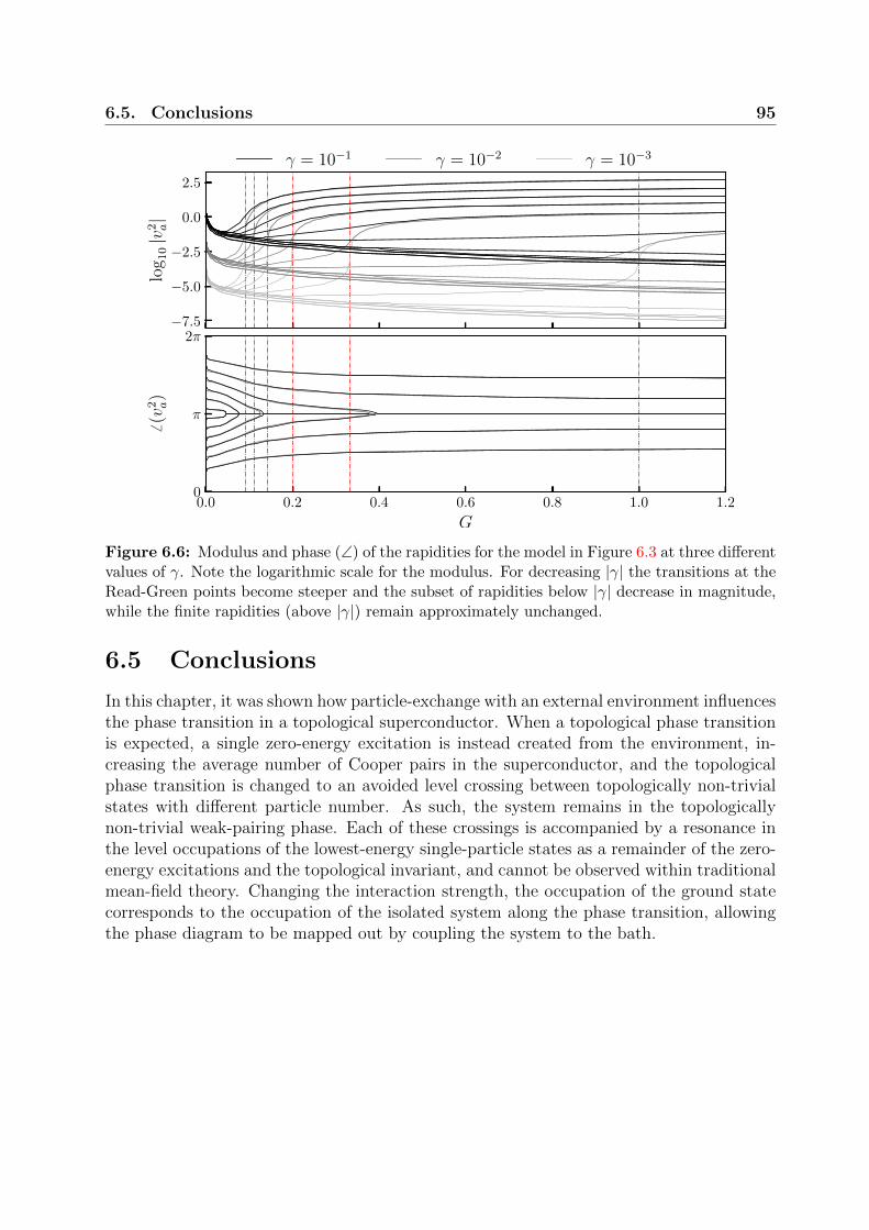
6.5. Conclusions 95
−7.5
−5.0
−2.5
0.0
2.5
log
10|v2 a|
0.0 0.2 0.4 0.6 0.8 1.0 1.2
G
0
π
2π
6 (v
2 a)
γ = 10−1 γ = 10−2 γ = 10−3
Figure 6.6: Modulus and phase (∠) of the rapidities for the model in Figure 6.3 at three differentvalues of γ. Note the logarithmic scale for the modulus. For decreasing |γ| the transitions at theRead-Green points become steeper and the subset of rapidities below |γ| decrease in magnitude,while the finite rapidities (above |γ|) remain approximately unchanged.
6.5 Conclusions
In this chapter, it was shown how particle-exchange with an external environment influencesthe phase transition in a topological superconductor. When a topological phase transitionis expected, a single zero-energy excitation is instead created from the environment, in-creasing the average number of Cooper pairs in the superconductor, and the topologicalphase transition is changed to an avoided level crossing between topologically non-trivialstates with different particle number. As such, the system remains in the topologicallynon-trivial weak-pairing phase. Each of these crossings is accompanied by a resonance inthe level occupations of the lowest-energy single-particle states as a remainder of the zero-energy excitations and the topological invariant, and cannot be observed within traditionalmean-field theory. Changing the interaction strength, the occupation of the ground statecorresponds to the occupation of the isolated system along the phase transition, allowingthe phase diagram to be mapped out by coupling the system to the bath.
Appendices
6.A Bethe equations
In this Appendix, the Bethe equations are derived for the commuting operators
Qk =(Szk +1
2) + γε−1
k S+k − λε−1
k S−k
−GL∑j 6=k
[εkεjε2k − ε2j
(S+k S−j + S−k S
+j
)+
2ε2jε2k − ε2j
(SzkS
zj −
1
4
)], (6.17)
which reduce to the conserved charges of the px + ipy model in the limiting case γ = −λ,but commute for arbitrary values of γ and λ, leading to possible non-Hermitian conservedcharges. The Bethe states are again product wave functions
|v1 . . . vL〉 =L∏a=1
S+(va) |0〉 , S+(va) = − λv2a
+G
L∑j=1
εjε2j − v2
a
S+j , (6.18)
with the set of rapidities va, a = 1 . . . L to be determined. The reference state is againgiven by |0〉 = |↓ . . . ↓〉, despite it not being an eigenstate of Qk for non-zero γ. This wavefunction does not contain a definite particle number due to the presence of the constantfactor λ/v2
a in the generalized creation operator S+(va). Alternatively, these can also beobtained from a non-Hermitian and non-symmetric GGA defined by the operators4
S+(u) = − λ
u2+G
L∑j=1
εjε2j − u2
S+j , S−(u) =
γ
u2+G
L∑j=1
εjε2j − u2
S−j (6.19)
Sz(u) = G
L∑j=1
εjε2j − u2
Szj . (6.20)
4The GGA from Ref. [157] can here be recovered in the rational limit.
96

6.A. Bethe equations 97
Because of the commutativity, all conserved operators again share a common set of eigen-states, and the conditions for the product state (6.18) to be an eigenstate of Qk can bederived. The action on the wave function can be determined through a Richardson-Gaudincommutator scheme as
Qk
L∏a=1
S+(va) |0〉 =L∑a=1
L∑b=a+1
(L∏
c 6=a,bS†(vc)
)[[Qk, S
+(va)], S+(vb)] |0〉
+L∑a=1
(L∏b6=a
S+(vb)
)[Qk, S
+(va)] |0〉+
(L∏a=1
S+(va)
)Qk |0〉 . (6.21)
The necessary commutation relations are given by
[Qk, S+(va)] = 2G2 εk
ε2k − v2a
S+k
(L∑j=1
v2a
ε2j − v2a
Szj
)+G
εkε2k − v2
a
S+k
(1 + 2G
L∑j 6=k
Szj
)
− 2Gv2a
ε2k − v2a
S+(va)Szk ,
[[Qk, S+(va)], S
+(vb)] = 2G2 εkv2a − v2
b
S+k
[v2a
ε2k − v2b
S+(va)−v2b
ε2k − v2a
S+(vb)
]. (6.22)
Taking these results together, the action of a single conserved operator on the productwave function can be written as
Qk
L∏a=1
S+(va) |0〉 =
[G
L∑a=1
v2a
ε2k − v2a
]L∏a=1
S+(va) |0〉+ γε−1k S+
k
L∏a=1
S+(va) |0〉
+GL∑a=1
εkε2k − v2
a
[(1 +G)−G
L∑j=1
ε2jε2j − v2
a
+ 2GL∑b6=a
v2b
v2b − v2
a
]S+k
L∏b6=a
S+(vb) |0〉 .
(6.23)
In order to be an eigenstate, the two unwanted (non-diagonal) terms should cancel. It canbe shown that the contributions from different excitation sectors cancel termwise providedthe rapidities v1 . . . vL satisfy a set of Bethe equations. First, the contribution from bothterms to the state S+
k |0〉 containing a single excitation is checked, which vanishes providedthe set of equations
L∑a=1
ε2kv2a
ε2k − v2a
[(1 +G)−G
L∑j=1
ε2jε2j − v2
a
+ 2GL∑b 6=a
v2b
v2b − v2
a
]=γλ
G, (6.24)
are satisfied. These can be brought in the previously-obtained form [184]
(1 +G)−GL∑j=1
ε2jε2j − v2
a
+ 2GL∑b 6=a
v2b
v2b − v2
a
=γλ
G
∏Lj=1(v−2
a − ε−2j )∏L
b 6=a(v−2a − v−2
b ), (6.25)

98 Chapter 6. Read-Green resonances
by interpreting (6.24) as a matrix-vector multiplication and multiplying with the well-known inverse of a Cauchy matrix (see Chapter 4). However, this requirement only cancelsa single contribution from both unwanted terms, when all other contributions should alsocancel exactly in order for (6.18) to be an eigenstate. Remarkably, this leads to a set ofequivalent equations. The coefficient in front of a state with N + 1 excitations where theset of spins labeled k, i(1), . . . , i(N) are flipped up is proportional to
CNk,i(1),...,i(N) =
L∑a=1
Fa
ε−2k − v−2
a
∑A∈SNa
1∏Nc=1(ε−2
i(c) − ν−2c )
+γλ
G
[∑A∈SN
1∏Nc=1(ε−2
i(c) − ν−2c )
],
(6.26)
with
Fa = (1 +G)−GL∑j=1
ε2jε2j − v2
a
+ 2GL∑b 6=a
v2b
v2b − v2
a
(6.27)
and SNa the set of N -tuples built out of N non-repeated elements v1, . . . va−1, va+1, . . . , vLand SN the set of N -tuples built from v1, . . . , vL. The elements of these sets are denotedA = ν1, . . . , νN and A = ν1, . . . , νN. A highly similar expression was obtained in thestudy of the DJCG models, where it was proven that these expressions vanish providedthe Bethe equations are satisfied [155]. The full proof that (6.26) equals zero is completelyanalogous and does not depend on the explicit form of the Bethe equations, rather on theCauchy-matrix structure when evaluating Fa as in Eq. (6.24) and plugging this in Eq.(6.26). Following Ref. [155], this then reduces to a purely combinatorial problem.

CHAPTER 7
Variational application of the Bethe ansatz
All models are wrong, but some are useful.
George E.P. Box
While integrable models can be solved exactly in a polynomial time, this advantagecomes at a price – for a model to be integrable, and thus exactly solvable, all parametersand interactions of the system need extraordinary fine-tuning. Even slight perturbationsto the Hamiltonian break integrability, and it is still an open question how much of thefeatures of integrability are retained for systems ‘close to integrability’. Theoretically, weimmediately lose the full underlying framework, and it is in general no longer possible tosolve such systems using Bethe ansatz techniques.
It is then a natural question to ask how well the wave functions of systems close tointegrability can be approximated using exact eigenstates of integrable systems. In thischapter, we propose to perform a variational optimization within the set of eigenstates ofintegrable Richardson-Gaudin models in order to obtain the optimal approximation to theground state of a given Hamiltonian. While this method cannot be expected to returnaccurate approximations to ground states of arbitrary Hamiltonians, it is tailor-made formodels which are in some sense ‘close to’ Richardson-Gaudin integrable models. In suchmodels, the approximations can be made clearer and the advantages and limitations of theintegrable wave functions can be better understood.
The main requirement for any variational method to be feasible is being able to effi-ciently and accurately calculate and minimize the energy functional
E [ψ] =〈ψ|H|ψ〉〈ψ|ψ〉 , (7.1)
for any given Hamiltonian H and any given trial state |ψ〉 [7]. As shown in the firsthalf of this thesis, the theoretical and numerical toolbox of integrability provides us with
99

100 Chapter 7. Variational application of the Bethe ansatz
exactly this. Following Chapter 4, the expectation value of a given Hamiltonian can beevaluated as a sum of determinants. These can be evaluated at a computationally favorable(polynomial) scaling, and a gradient descent method can be applied to minimize the energyfunctional [145].
Here, this method is applied to spin systems consisting of an integrable model plus anintegrability-breaking perturbation term. If no integrability-breaking terms are present, theproposed method leads to the exact ground state by construction. Furthermore, thanksto the use of eigenstates of unperturbed integrable models as trial states, the variationalenergy is also guaranteed to be an improvement upon the energy obtained from first-orderperturbation theory, serving as further motivation for the choice of trial states. The specificclass of Richardson-Gaudin integrable models then provides a large amount of variationalparameters and a wide variety of physical systems [53].
It is shown that this method is also able to return accurate approximations in the regionwhere perturbation theory is not expected to hold, provided the perturbative interactionsdo not influence the qualitative physics of the model. In this case, the bulk of the corre-lations in the ground state of the non-integrable system is captured by the ground stateof the integrable system, and the variational optimization returns an accurate approxima-tion. If this is not the case, it is shown that a more accurate description can be obtainedby variationally optimizing an excited state of an integrable model. This is illustrated bycomparing overlaps and correlation functions, and can be understood as (avoided) levelcrossings in the spectrum of the non-integrable Hamiltonian [60], when the perturbativeenergy of an excited state drops below that of the original ground state.
In a broader context, this research fits within the general development of wave function-based methods (as compared to density-based methods) for the description of strongly-correlated models. In this aspect, this approach is also motivated by recent developmentsin the theory of Antisymmetric Product of Geminals (APG) in molecular physics andquantum chemistry [216–219]. Composed as a generalized valence-bond wave function,APG wavefunctions are tailor-made for the description of resonating electron-pair con-figurations, and tie in directly with the Lewis picture of molecular bonding. Recently,it has been realized that the Richardson-Gaudin eigenstates fit within the class of gemi-nal wave functions. This has given rise to various computationally tractable versions ofAPG, including a variational formulation based on the Richardson-Gaudin wave functions[219, 220]. However, initial calculations for simple molecular systems [219] showed thatthe variational method was surpassed in accuracy and efficiency by Coupled-Cluster-basedAPG methods [218, 221]. These preliminary results then naturally shifted the researchfocus to the Coupled-Cluster variant of APG theory in recent years [221–226]. However, itis presently becoming clear that further developments in APG theory will benefit from awell-defined Hilbert space, which is conveniently obtained through the connection with avariational Richardson-Gaudin APG state and the associated integrable Hamiltonian. Thisthen paves the way for an extension of the variational method by including excitations ontop of the variational approximation, as discussed in the second half of this chapter. Thepresent chapter is largely based on Refs. [227, 228].

7.1. Moving away from integrability 101
7.1 Moving away from integrability
A rich variety of methods has been developed for the approximation of the ground state ofgeneral non-integrable systems. Here, the distinction can be made between wave function-based methods such as mean-field theory [6], the related coupled cluster and configurationinteraction theories [9], tensor networks [10] and variational quantum Monte Carlo methods[229], as compared to density-based density functional theory [230]. Within the wavefunction-based methods, the common approach is that a specific structure is imposed ona wave function, which is then optimized (often variationally) in order to approximate theground state of a given system [7]. The success of any approach is then judged by howwell the proposed structure of the wave function matches that of the exact ground state.
In this chapter, the Bethe states |ψRG〉 from rational Richardson-Gaudin models (2.56)will be investigated as variational ansatz, where
|ψRG〉 =N∏a=1
(L∑i=1
S+i
εi − va
)|↓ . . . ↓〉 , (7.2)
the different spins in the system are labeled i = 1, . . . , L and the spin operators constitutean su(2) algebra (see Chapter 2). Although the parameters ε1 . . . εL and v1 . . . vN havea clear physical interpretation within integrability, these can be thought of as arbitraryparameters when regarding (7.2) as a variational ansatz. In order to obtain the computa-tionally favourable scaling from integrability following Chapter 4, the state must be on-shelland the variables are coupled through the Bethe (or Richardson-Gaudin) equations (4.10).It is worth stressing that although all variables in the wave function can be connected tothe physics of integrable systems, it is not strictly necessary to interpret them as such.They can equally be treated as variational parameters. Given the Hamiltonian H of astrongly-correlated system, the goal is now to find the Bethe state minimizing the energy(7.1), resulting in a variational energy
EVar. = minE [ψRG] . (7.3)
For such a generalized product state to be computationally tractable, it needs to be dressedwith additional structure, which is here provided by integrability and the on-shell require-ment. It is worth noting that the projected BCS method can be reinterpreted as a specialcase of variational RG integrability, providing a connection between the variational wavefunction (7.2) and the BCS mean-field wave function [99]. Systems successfully describedby mean-field theory, where the particles can be treated as non-interacting particles, alsoarise as a particular limit of the Bethe ansatz. In fact, a crucial feature of the wavefunction (7.2) is that it exhibits a similar product structure as the Hartree-Fock wave func-tion [7], returning a Slater determinant in the non-interacting limit g → 0 (see Chapter2). The variational method can thus already be expected to return accurate results forweakly-correlated systems.
The key question is then if the on-shell condition restricts the physics that can becaptured by this ansatz. While integrable Hamiltonians are necessarily quite schematic,

102 Chapter 7. Variational application of the Bethe ansatz
they have shown remarkable success in the description of general physical phenomena.Richardson’s original solution to the (reduced) BCS Hamiltonian [28, 29] already suc-ceeded in qualitatively describing regular superconductivity [16, 33], and only afterwardswas it recognized that this Hamiltonian is integrable [36]. Furthermore, form factors inintegrable theories are exactly known, and can be used to build a perturbation theoryfor non-integrable models [43–48]. Approximate scattering matrices for low-lying excitedstates of non-integrable systems have also been constructed from approximate (coordinate)Bethe ansatz techniques [49–52]. Despite these models being non-integrable, accurate re-sults could still be obtained by applying techniques from integrability. Integrability-basedmethods have also been proposed in the description of time evolution governed by an in-tegrable Hamiltonian plus a perturbation, both in the description of the initial behaviour[77, 231] and the infinite-time behaviour [232] of observables. Such problems have alsobeen tackled using a numerical renormalization group expressed in the basis of eigenstatesof the integrable model [233].
The majority of these results essentially build on the same idea as our proposed method– integrability can be used to describe the bulk of the correlations, on which correctionscan be added. While using the same technical toolbox as these methods, our results aremainly similar in spirit to the use of perturbation theory for non-integrable system, wherethe important distinction is that the variational optimization guarantees a more accurateapproximation of the ground state wave function than perturbation theory.
7.2 A variational method
The procedure is conceptually straightforward. For a given Hamiltonian
H = Hint + V, (7.4)
with Hint an integrable (Richardson-Gaudin) Hamiltonian, and V containing additionalinteractions breaking the integrability, we wish to minimize
E [ψRG] =〈ψRG|H|ψRG〉〈ψRG|ψRG〉
. (7.5)
It is important to note that the variables in the wave function are independent from those inthe integrable Hamiltonian Hint, since the former are the degrees of freedom over which weoptimize, while the latter are a characteristic of the unperturbed system. Obviously, in thelimit of a vanishing perturbation V = 0 the Hamiltonian H = Hint becomes integrable, andthe variational optimization should return the variables in the Hamiltonian as variationalparameters, since this wave function is then the exact ground state of the integrable Hamil-tonian. While these states explicitly depend on L+N variables ε1 . . . εL and v1 . . . vN,the demand that these states are on-shell (4.10) leaves L degrees of freedom over which tooptimize, which can be chosen as ε1 . . . εL, and we denote E[ψRG] ≡ E[ε1 . . . εL] ≡ E[~ε],with the implicit assumption that all rapidities v1 . . . vN uniquely follow through the

7.3. Results 103
Bethe equations, resulting in a manifold of states only determined by the variables ~ε.However, an additional discrete degree of freedom exists – the choice of eigenstate. Eacheigenstate of an integrable Hamiltonian defined by a set of variables ~ε can be written as(7.2), so the targeted eigenstate needs further specification. This degree of freedom willinitially be disregarded, and we will restrict ourselves to the state that is adiabaticallyconnected to the ground state of the integrable Hamiltonian in the limit of a vanishingperturbation. For small perturbations, it is expected that this state will be the most rel-evant. Later, it will be shown that this choice is not guaranteed to be optimal for largeperturbations, and the excited states will prove to be important.
7.3 Results
7.3.1 Perturbing the central spin model
The results will first be illustrated on the central spin model (see Section 2.7.1) with per-turbations restricted to operators acting on one or two spins. The central spin Hamiltonianis given by
Hcs = BzSz1 + g
L∑i 6=1
~S1 · ~Siε0,1 − ε0,i
, (7.6)
describing the interaction of a single spin on which a magnetic field B is applied, with a bathof surrounding spins. This model is integrable for any choice of the interaction modulatedby ε0,i, which has been written in this way in order to make this connection explicit. Inthis model, the bath spins do not interact among themselves and do not experience themagnetic field applied to the central spin. However, such interactions may be added in aperturbative way by introducing terms of the form Szi and ~Si · ~Sj in the Hamiltonian. Thebasic physics in this model can be easily understood – Bz determines the orientation of thecentral spin 〈Sz1〉, either parallel or anti-parallel to the quantization axis, while the signs
of g/(ε0,1− ε0,i) determine the relative orientation of the bath spin ~Si with the central spin
〈~S1 · ~Si〉.In the following, system sizes L = 12 are considered for which exact diagonalization
methods can still be used as benchmark and the Hamiltonian is parametrized with ε0,i =L−i as a picket-fence model [135]. This leads to algebraically decaying interactions betweenthe central spin and the bath spin, where the strength of the interaction is fixed by settingBz = 1 and g = −2, intermediate between strong- and weak-coupling [124]. For thischoice of parametrization, the central spin and all surrounding spins tend to align, whilealso being restricted by conservation of spin projection Sz =
∑i S
zi . In the following, we
always choose Sz = 0 (or L = 2N), since this is the sector where the dimension of theHilbert space is maximal.
Single-spin perturbation. Firstly, calculations are performed for a Hamiltonian
H = Hcs + µSzi , (7.7)

104 Chapter 7. Variational application of the Bethe ansatz
−1.0 −0.5 0.0 0.5 1.0
µ
−2.0
−1.8
−1.6
−1.4
〈H〉PT1
Var.
Exact
−1.0 −0.5 0.0 0.5 1.0
µ
0.75
0.80
0.85
0.90
0.95
1.00
〈ψ|ψEx.〉
PT0
Var.
Figure 7.1: Results for the central spin model with perturbation µSzi . Left: Variational energy(Var.), exact ground state energy (Exact), and first-order perturbation theory (PT1) energy fordifferent values of the perturbation strength. Right: Overlap of the exact ground state with thevariational ground state (Var.) and the ground state of the unperturbed model (PT0).
applying a magnetic field of size µ to one of the spins in the bath (here labeled i). Such amodel has previously also been investigated in the context of integrability-breaking [87, 88].The variational energy is calculated and compared with the ground-state energy obtainedby exact diagonalization. In Figure 7.1, we plot the variational energy (Var.), the exactground-state energy (Exact), and the energy obtained by first-order perturbation theory(PT1) for varying perturbation strengths µ, with i = 2 chosen to maximize the deviationfrom the integrable model, since the central spin interacts most strongly with this bath spin.Since the ground-state energy deviation is intimately connected to the overlap between theapproximate ground state and the exact ground state, this is also given in Figure 7.1. Asthe error in the energy is generally quadratic in the error in the overlap, the latter can beseen as a more sensitive measure for the accuracy of the proposed method.
Labeling the parameters of the unperturbed integrable model as ~ε0, the relevant energiescan be contrasted as
EVar. = min~εE [~ε] , EPT1 = E [~ε0] , (7.8)
making clear why the variational method provides a guaranteed improvement on first-orderperturbation theory. In the chosen model, perturbation theory is guaranteed to provide agood approximation to the exact ground state energy only when |µ 〈Szi 〉 | ∆E, with ∆Ethe energy difference between the ground state and the first excited state. In the following,this roughly corresponds to |µ| 1, which we will consider to be a small perturbation.
The overlaps given are those between the variationally obtained wave function (Var.)and the exact ground state, together with the overlap between the ground state of the

7.3. Results 105
−10 0 10
=(va)
0
5
10
<(v a
)
µ = −1.0
−10 0 10
=(va)
0
5
10
µ = −0.5
−10 0 10
=(va)
0
10
µ = 0
−10 0 10
=(va)
0
10
µ = 0.5
−10 0 10
=(va)
0
20
µ = 1.0
Figure 7.2: Variational parameters for the Hamiltonian (7.7). Position of ~ε (squares) and ~v(dots) for the variationally optimized wave function in the complex plane at different values ofthe perturbation strength. The white square denotes the variable εi associated with the level onwhich the perturbation is applied following Eq. (7.7).
unperturbed model and the exact ground state (PT0)1. The variational wave function isable to accurately model the ground state for a wide range of the perturbation strength,even going up to the limit where the size of the perturbation interaction equals that of theunperturbed central spin interaction (|µ| = 1), providing a substantial improvement overfirst-order perturbation theory. Here, the variational optimization plays a crucial role, ascan be seen by comparing the overlap of the exact ground state with the ground state of theunperturbed Hamiltonian to the overlap with the variationally optimized wave function,which is improved by several orders of magnitude (from an overlap of 0.7754 to 0.9908 forµ = −1). However, since the perturbation only acts on a single spin site, it is not expectedthat this will fundamentally influence the correlations in the model, and more intrusiveperturbations may be more physical.
Some more insight in the role of the optimization and the structure of the wave functioncan be obtained by considering the evolution of the variables ~ε and ~v in the wave function.These are given in Figure 7.2 for different values of the perturbation strength. The variables~ε are restricted to be real, while the rapidities ~v are either real or arise as complex conjugatepairs. The single-spin character of the perturbation is clear from these figures. Onlythe variable εi (i = 2), associated with the perturbed level, is significantly sensitive tothe perturbation, whereas all other variables are largely unaffected. While the on-shellcondition still connects both sets of variables, it can be seen that the variables ~v are quiterobust against perturbations. This also motivates the use of ~ε as variational parameters.
Double-spin perturbation. Secondly, and more interestingly, this method is applied
1The first-order correction to the energy (PT1) follows from the unperturbed wave function (PT0),hence the discrepancy in order.
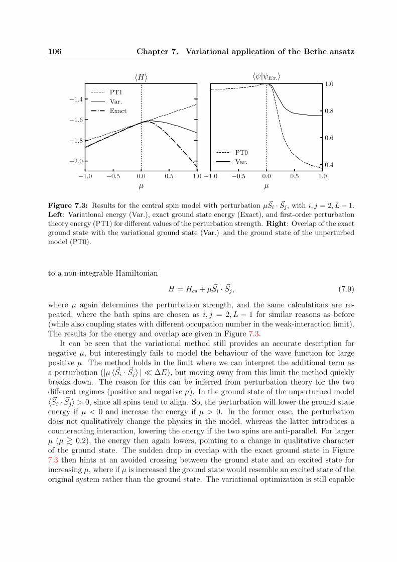
106 Chapter 7. Variational application of the Bethe ansatz
−1.0 −0.5 0.0 0.5 1.0
µ
−2.0
−1.8
−1.6
−1.4
〈H〉PT1
Var.
Exact
−1.0 −0.5 0.0 0.5 1.0
µ
0.4
0.6
0.8
1.0〈ψ|ψEx.〉
PT0
Var.
Figure 7.3: Results for the central spin model with perturbation µ~Si · ~Sj , with i, j = 2, L − 1.Left: Variational energy (Var.), exact ground state energy (Exact), and first-order perturbationtheory energy (PT1) for different values of the perturbation strength. Right: Overlap of the exactground state with the variational ground state (Var.) and the ground state of the unperturbedmodel (PT0).
to a non-integrable Hamiltonian
H = Hcs + µ~Si · ~Sj, (7.9)
where µ again determines the perturbation strength, and the same calculations are re-peated, where the bath spins are chosen as i, j = 2, L − 1 for similar reasons as before(while also coupling states with different occupation number in the weak-interaction limit).The results for the energy and overlap are given in Figure 7.3.
It can be seen that the variational method still provides an accurate description fornegative µ, but interestingly fails to model the behaviour of the wave function for largepositive µ. The method holds in the limit where we can interpret the additional term asa perturbation (|µ 〈~Si · ~Sj〉 | ∆E), but moving away from this limit the method quicklybreaks down. The reason for this can be inferred from perturbation theory for the twodifferent regimes (positive and negative µ). In the ground state of the unperturbed model
〈~Si · ~Sj〉 > 0, since all spins tend to align. So, the perturbation will lower the ground stateenergy if µ < 0 and increase the energy if µ > 0. In the former case, the perturbationdoes not qualitatively change the physics in the model, whereas the latter introduces acounteracting interaction, lowering the energy if the two spins are anti-parallel. For largerµ (µ & 0.2), the energy then again lowers, pointing to a change in qualitative characterof the ground state. The sudden drop in overlap with the exact ground state in Figure7.3 then hints at an avoided crossing between the ground state and an excited state forincreasing µ, where if µ is increased the ground state would resemble an excited state of theoriginal system rather than the ground state. The variational optimization is still capable

7.3. Results 107
0.0 0.2 0.4 0.6 0.8 1.0
µ
−2.0
−1.8
−1.6
−1.4
−1.2
〈H〉PT1
Var.
Exact
PT1 - Exc.
Var. - Exc.
0.0 0.2 0.4 0.6 0.8 1.0
µ
0.0
0.2
0.4
0.6
0.8
1.0〈ψ|ψEx.〉
PT0
Var.
PT0 - Exc.
Var. - Exc.
Figure 7.4: Results for the central spin model with perturbation µ~Si · ~Sj . Left: Variationalenergy (Var.), exact ground state energy (Exact), and first-order perturbation theory energy(PT1) starting from the ground and excited state of the integrable model for different values ofthe perturbation strength. Right: Overlap of the exact ground state with the variational groundstate (Var.) and the ground state of the unperturbed model starting from both the ground andexcited state of the integrable model (PT0).
of increasing the overlap by more than a factor 2, but is ultimately unable to obtain anaccurate description for large µ. This can be understood since, while the perturbationincreases the energy of the unperturbed ground state, it simultaneously lowers the energyof selected excited states of the unperturbed model.
For relatively simple perturbations, the relevant excited state can be gathered from thelimit |µ| → ∞, where the perturbation becomes dominant, and the state which is adiabati-cally connected to this excited state in the limit µ→ 0 can be variationally optimized. Forpositive µ, the results for a variational optimization starting from both the ground stateand this excited state are presented in Figure 7.4. At small µ, the unperturbed groundstate is the energetically favourable one, while for increasing perturbation strength theenergy of the unperturbed excited state drops below that of the unperturbed ground state.Such crossings are observed both in perturbation theory and in the variational method,albeit occurring for smaller values of the perturbation in the variational method. This be-haviour can also be observed from the overlaps, where a similar crossing occurs in the sameregion. The variational optimization again plays an important role in lowering the energyand increasing the overlap, both for the variational state obtained from the unperturbedground- and excited state, resulting in an improved approximation to the ground state.Note that, while this results in a much improved description, there is still a part of thewave function that cannot be captured by the variational method, and for which eitherperturbation theory would need to be applied on the optimized wave function, or a multi-reference approach should be implemented with multiple Bethe ansatz wave functions in

108 Chapter 7. Variational application of the Bethe ansatz
−10 0 10
=(va)
0
10
<(v a
)
µ = −1.0
−10 0 10
=(va)
0
10
µ = −0.5
−10 0 10
=(va)
0
10
µ = 0
−10 0 10
=(va)
−20
0
µ = 0.5
−10 0 10
=(va)
−50
0
µ = 1.0
Figure 7.5: Variational parameters for the Hamiltonian (7.9). Position of ~ε (squares) and ~v(dots) for the variationally optimized wave function in the complex plane at different values ofthe perturbation strength. The white squares denote the variables εi, εj associated with the levelson which the perturbation is applied following Eq. (7.9).
the variational optimization.
The structure of the optimized variables ~ε and ~v can again be analyzed (Figures 7.5 and7.6). The two-spin character of the interaction is clearly visible, where the optimizationis mainly sensitive to the two variables εi, εj (i = 2, j = 11) in the region where theoptimization performs well. When the optimization fails to provide an accurate wavefunction, the rapidities exhibit a qualitative change (complex conjugate variables becomereal) and quickly increase in absolute value, pointing out that they are qualitatively wrong.Starting from the excited state in the unperturbed model, it is observed that the rapiditiesalready have the correct structure, and remain bounded during the optimization.
Some more physical insight can be gathered from expectation values and correlationcoefficients calculated from both wave functions. In Figures 7.7 and 7.8, we present theexpectation values 〈~Si · ~Sj〉 , ∀i, j, motivated by the choice of perturbation interactions, andthe unconnected correlation coefficients σij = 〈Szi Szj 〉 − 〈Szi 〉 〈Szj 〉 ,∀i, j for both exact andvariational wave functions at different values of µ. It is clear that the correlations withinthe wave function only change slightly for negative µ, and as such the wave function isable to easily adapt to the perturbation. Comparing the exact and the variational groundstate for positive µ, it is notable that the correlations between the two spins affected bythe interactions have not been captured by the variational ground-state wave function.Comparing this with the results from the variational excited wave function, it can be seenthat the missing correlations are reintroduced there, as was expected.
For low perturbation strengths, the variational wave function is able to adapt to thecorrelation structure of the exact ground state through the optimization. The change incorrelation coefficients also points towards the failure of perturbation theory. In the regionµ & 0.2, the unconnected correlation coefficients from the approximate wave function for

7.3. Results 109
−10 0 10
=(va)
0
5
10
<(v a
)
µ = 0
−10 0 10
=(va)
0
10
µ = 0.5
−10 0 10
=(va)
0
10
µ = 1.0
Figure 7.6: Results for the central spin model with perturbation µ~Si · ~Sj . Position of ~ε (squares)and ~v (dots) for the variationally optimized wave function starting from an excited state in thecomplex plane at different values of the perturbation strength. The white squares denote thevariables εi, εj associated with the levels on which the perturbation is applied.
the levels on which we apply the perturbation vanish, and this level effectively decouplesfrom the many-body system. In the exact wave function, this decoupling does not occur andinstead these coefficients change sign. From this, it can be concluded that the wave functioncan adapt to the perturbation for as long as the general structure of the correlations doesnot change. By starting the variational optimization from the excited state, the correctstructure is again recovered, as can be seen in the bottom row of Figures 7.7 and 7.8.
This can now also be related to the expected range of applicability of perturbationtheory. For the given Hamiltonians H = Hcs + µV , perturbation theory starting from theintegrable µ = 0 limit can be expected to provide accurate results only if |µ 〈V 〉 | ∆E,in the regime where the additional term can be considered a small perturbation on theintegrable model. The variational optimization starting from the ground state resultsin a relatively accurate approximation for a larger range of µ, even when the additionalterm can no longer be considered to be a small perturbation, provided there occur noavoided crossings between the ground- and excited states of the integrable Hamiltonianin the spectrum of the non-integrable Hamiltonian when the perturbation strength µ isadiabatically increased from 0 to the given value. Because these Hamiltonians are non-integrable these are expected to be avoided crossings, but this reasoning should also holdfor allowed level crossings.
It can be checked that the same behaviour is observed when introducing more in-volved perturbations, where small perturbations can be accurately described starting fromthe ground state of the integrable Hamiltonians, and for larger perturbations variationaloptimization starting from an excited state is necessary in order to obtain the optimalapproximative state. However, at present it is not always clear which excited state shouldbe chosen for arbitrary perturbations. In practice, this problem could be circumvented

110 Chapter 7. Variational application of the Bethe ansatz
Exact
Var.
µ = −1
Var.
-E
xc.
µ = −0.5 µ = 0 µ = 0.5 µ = 10.00
0.15
0.30
0.45
0.60
0.75
Figure 7.7: Absolute value of the expectations values 〈~Si · ~Sj〉 for the central spin model with
perturbation µ~Si ·~Sj , with i, j = 2, L−1. The expectation values are taken w.r.t. the exact groundstate and the variational state obtained by starting from both the ground state and excited stateof the unperturbed model.
Exact
Var.
µ = −1.0
Var.
-E
xc.
µ = −0.5 µ = 0 µ = 0.5 µ = 1
−0.16
−0.08
0.00
0.08
0.16
Figure 7.8: Correlation coefficients 〈Szi Szj 〉−〈Szi 〉 〈Szj 〉 for the central spin model with perturba-
tion µ~Si · ~Sj , with i, j = 2, L−1. These correlation coefficients are calculated for the exact groundstate and the variational state obtained by starting from both the ground state and excited stateof the unperturbed model.

7.3. Results 111
−1.0 −0.5 0.0 0.5 1.0
µ
−50
−40
−30
〈H〉PT1
Var.
Exact
−1.0 −0.5 0.0 0.5 1.0
µ
0.85
0.90
0.95
1.00
〈ψ|ψEx.〉
PT0
Var.
Figure 7.9: Results for the inhomogeneous BCS model. Left: Variational energy (Var.), exactground state energy (Exact), and first-order perturbation theory (PT1) for different values of theperturbation strength. Right: Overlap of the exact ground state with the variational groundstate (Var.) and the ground state of the unperturbed model (PT0).
using a stochastic approach, since it was found that several excited states can lead to thesame variationally optimized state.
7.3.2 Perturbing the Richardson model
The other emblematic example of Richardson-Gaudin models is the Richardson Hamilto-nian (see Section 2.7.2) as given by
HBCS =L∑i=1
εiSzi + g
L∑i,j=1
S+i S−j . (7.10)
This Hamiltonian can be used to describe fermion pairing in e.g. nuclear pairing and su-perconductivity [94], and is exactly solvable under the key assumption that the pairinginteractions are uniform and fully determined by a single pairing constant g [28, 29]. Be-cause of this exact solvability, this model has recently become a testing ground for novelmany-body methods focusing on pairing interactions [226, 234–236]. It’s worthwhile tostress that the proposed integrability-based method will return the exact ground stateenergy of this model by construction. Moving away from integrability, the restriction ofuniform interactions can be relaxed by introducing non-uniformities in a perturbative way,resulting in a more physical model. The Hamiltonians under consideration are of the form
HBCS =L∑i=1
εiSzi +
L∑i,j=1
GijS+i S−j . (7.11)

112 Chapter 7. Variational application of the Bethe ansatz
−10 0 10
=(va)
0
5
10
<(v a
)
µ = −1.0
−10 0 10
=(va)
0
5
10
µ = −0.5
−10 0 10
=(va)
0
10
µ = 0
−10 0 10
=(va)
0
10
µ = 0.5
−10 0 10
=(va)
−10
0
10
µ = 1.0
Figure 7.10: Results for the inhomogeneous BCS model. Position of ~ε (squares) and ~v (dots)for the variationally optimized wave function in the complex plane at different values of theperturbation strength.
While such models are solvable by U(1)-breaking BCS mean-field theory in the thermody-namic limit, it is important to obtain an accurate description for medium-size systems aswell [226, 235, 236]. In fact, it has been shown that the Richardson-Gaudin equations areequivalent to the BCS mean-field equations for thermodynamically large systems, and assuch the BCS wave function and the Bethe ansatz wave function coincide in this limit [99].The results are presented in Figure 7.9 for a single Richardson Hamiltonian with interac-tion matrix Gij = g + µgij, with g = −1 and gij random numbers uniformly distributedover the interval [0, 1]. We again take system size L = 12, parameters according to thepicket-fence model, and take L = 2N corresponding to half-filling.
The same behaviour as for the central spin model can be observed, where it should benoted that the error on the energy and overlap is much smaller compared to the resultsfor the central spin model. This implies that a general pairing Hamiltonian can alreadybe efficiently approximated by taking the average pairing interaction as single parameter,consistent with the success of BCS mean-field theory in the description of such Hamilto-nians. From the structure of the optimized wave function (Figure 7.10), it can be seenthat only minor modifications are necessary in order for the wave function to provide anaccurate description.
7.3.3 Discussion
At present, the selection of the proper excited state on which to perform the variationaloptimization is the main bottleneck in the procedure. One can envision several meth-ods to cope with this problem. The method used in this chapter is to capitalize on thephysical insight in the perturbation. Often, the integrability-breaking term in the Hamil-tonian itself has a clear physical interpretation, and it is only the competition between

7.4. Richardson-Gaudin Configuration Interaction 113
the integrable and non-integrable part of the Hamiltonian which is the main cause forcomplications. Consequently, the correct choice of variational manifold among the excitedstates can be deduced from the ground state structure of the integrability-breaking term.Other approaches could make use of ideas of stochastic sampling, the correspondence withCoupled-Cluster approaches [218, 221–226] or the pp-TDA adiabatic connection [124, 202].In practice, all relevant excited states were obtained as so-called 1p-1h or 2p-2h excitationsof the ground state [92].
7.4 Richardson-Gaudin Configuration Interaction
Given the remarkable accuracy of the variational approach in the description of generalpairing Hamiltonians, this method can be extended by including an increasing numberof Bethe states in the ansatz. The exact ground states of all models have a clear multi-reference character in the basis of Slater determinants, and given the similarity of the Bethestate to a Slater determinant it is now possible to construct the multi-reference characterof exact ground states in the basis of (variationally optimized) Bethe states. This wouldthen lead to a more accurate description of both the ground state and the lowest-lyingexcited states, extending the variational scheme to a two-part process.
1. In a first step, a variational Richardson-Gaudin calculation is performed. Because ofthe integrability of the underlying model, the variationally obtained state not onlygives an approximation to the ground state, but also a complete set of orthogonalbasis states, leading to an optimized basis used in the consecutive step.
2. In the second step, the actual Configuration Interaction (CI) step, the non-integrableHamiltonian of interest is diagonalized in an increasingly large basis set until conver-gence is obtained. This step is very much related to other CI methods acting in abasis of on-shell integrable states, such as the Truncated Space Approach [237–239]which has been used to diagonalize perturbed integrable quantum field theories inone dimension. In this work, the use of an optimized Richardson-Gaudin basis is key.
This then yields an approximation to both the ground state and the lowest-lying excitedstates, where both steps will be discussed in more detail in the following subsections. Thismethod can be seen as an adaptation of traditional HF+CI methods. In these methods, anoptimal single-particle Hartree-Fock (HF) product state is obtained first. This state thendefines a Fock Hilbert space in which residual interactions can be systematically includeduntil convergence. Again, the main difference in this work is that the HF state is replacedby a variational Richardson-Gaudin state, already incorporating pairing correlations in theinitial step.
7.4.1 Nuclear pairing models
This scheme will now be applied to a more realistic nuclear-pairing Hamiltonian describingthe Sn region. In such models, nuclear pairing correlations are traditionally incorporated

114 Chapter 7. Variational application of the Bethe ansatz
g7/2 d5/2 s1/2 h11/2 d3/2
Ωi 8 6 2 12 4εi −6.121 −5.508 −3.891 −3.778 −3.749g7/2 −0.2463 −0.1649 −0.1460 −0.2338 −0.1833d5/2 −0.2354 −0.1995 −0.2250 −0.3697s1/2 −0.7244 −0.1741 −0.2486h11/2 −0.1767 −0.1762d3/2 −0.2032
Table 7.1: Pairing interaction parameters εi and Gij in the Hamiltonian (7.12) for Sn isotopesfrom a G-matrix formalism [242, 243]. All energies are measured in MeV.
from symmetry-broken Bardeen-Cooper-Schrieffer (BCS) theory. However, as nuclear in-teractions are becoming better constrained and more accurate [240], this mean-field de-scription will no longer be sufficient, and many-body methods are urged to follow along.Ripoche et al. [235] recently argued for a method that combines symmetry projection andCI for pairing correlations, producing ground-state correlation energies with an accuracy of0.1% and better. The core idea is to construct an optimized set of basis states built fromthe projected BCS state and selected quasi-particle excitations, which are subsequentlyused in a non-orthogonal CI method. This can be quite well understood physically, be-cause the pairing correlations have already been optimized in the basis states, either at theBCS mean-field level in the strong interaction regime, or at the perturbative particle-holelevel in the weak interaction regime. As such, the approach can be regarded as a naturalgeneralization of the Polynomial Similarity Transformation method (PoST) [226], a many-body method that interpolates between projected BCS theory and pairs Coupled-ClusterDoubles (pCCD) [224]. The differences between Refs. [235] and [226] is that the formeremploys a non-orthogonal CI method, whereas the latter is based on a Coupled Clusterformulation of projected BCS [241]. Again, Bethe states from a variational Richardson-Gaudin calculation can also be used as an orthogonal set of basis states, further buildingon these ideas.
The nuclear pairing Hamiltonian can generally be written as
H =L∑i=1
εini +L∑
i,j=1
GijS+i S−j , (7.12)
where the effective pairing interaction can be obtained from a G-matrix construction for theSn isotopes in the neutron valence shell A = 100−132 (g7/2, d5/2, s1/2, h11/2, d3/2) [242, 243].The specific values of the pairing interaction can be found in Ref. [243], and are also listedin Table 7.1 for quick reference.
This is an ideal benchmark system for multiple reasons. First, the pairing strength isknown to be very stable in the Sn isotopes, with a slight experimentally-observed decreasearound the neutron number 64 subshell closure [244–246]. Second, the dimensions of the

7.4. Richardson-Gaudin Configuration Interaction 115
pairing Hamiltonian (7.12) are rather limited for this shell, so a comparison with exactresults from conventional exact CI remains possible [247]. To illustrate the performance ofthe effective interaction (Table 7.1) with respect to experimental values, calculated 3-pointneutron pairing gaps, derived from nuclear binding energies BE(A,Z) [248],
∆(3)(A,Z) = (−)A[BE(A,Z)− 2BE(A− 1, Z) +BE(A− 2, Z)], (7.13)
are compared to experimental values taken from [249] in Figure 7.11. For the purpose ofthis work, it is sufficient to note the qualitative agreement between the G-matrix resultsand experimental values within their errorbars. As such, this interaction will be used solelyto test the RGCI method, as is done before with other methods like [234, 250], and we willrefrain explicitly from making further comparison with experimental data.
100 105 110 115 120 125 130 135
A
1000
1500
2000
2500
3000
3500
4000
∆(3
) (A,Z
)[k
eV]
G-matrix
exp
Figure 7.11: 3-point neutron pairing gaps ∆(3) (7.13) calculated from an effective G-matrixinteraction (See Table 7.1 and Ref. [243]), and compared with experimental values [249].
The two-part process is now presented in Figures 7.12a and 7.12b. Because of theremarkable success of the variational approach for pairing models, the initial variationaloptimization can be restricted to the pairing strength g, while the single-particle energiesεi are fixed and taken to be those from Table 7.1. This has several advantages. First,the variational optimization of E[ψRG] = E[g] is reduced to a line-search compared toa gradient descent method. Second, the connection with HF mean-field theory can bemade more explicit, where the variationally-optimized pairing strength g0 and the resultingreduced BCS Hamiltonian
H =L∑i=1
εini + g0
L∑i,j=1
S+i S−j (7.14)
can be seen as a mean-field pairing description of the original Hamiltonian (7.12). Thisfirst step is illustrated in Figure 7.12a. The lowest full curve corresponds to the energy

116 Chapter 7. Variational application of the Bethe ansatz
−1.0 −0.8 −0.6 −0.4 −0.2 0.0
g
−97
−96
−95
−94
−93
−92
−91
−90
−89
E[M
eV]
En(exact)
En[g]
−4
−3
−2
−1
0
1
2
3
Ec
[MeV
]
(a)
0 25 50 75 100dim Hn
10−9
10−8
10−7
10−6
10−5
10−4
10−3
10−2
10−1
100
δ x
g = 0.000
g = −0.100
g = −0.500
g = −0.211
g = −0.322
g = 0.000
g = −0.100
g = −0.500
(b)
Figure 7.12: (a) Full lines represent the energy function profiles En[g] for different eigenstates nof the corresponding RG Hamiltonian (7.14). Exact eigenstate energies En(exact) of the effectiveHamiltonian (7.12) are given in dashed lines (n = 0 . . . 5). The energy scale shows total (left axis)and correlation energies (right axis). The calculations are performed for N = 8 pairs (116Sn).(b) Convergence rate of missing correlation error δc for the RGCI method with N = 8 (116Sn).Convergence rates for different integrable bases are denoted by the corresponding value of g.Units of g are given in MeV, and δc is dimensionless.
functional of the Richardson-Gaudin ground state, and gives the best approximation of theexact ground-state energy, as was expected. The variationally obtained energy is reachedat g0 = −0.211 MeV, giving rise to E[g0] = −95.907 MeV, which is equivalent to 99.07%of the exact correlation energy. A more practical measure for gauging the quality of amethod is given by 1 minus this correlation-energy ratio, being
δc = 1− Ec(method)
Ec(exact), (7.15)
which in the present example amounts to 0.93%. Apart from the ground-state energycurve E[g] ≡ E0[g], it is also interesting to investigate the performance of other Betheeigenstates energy curves. These are also included in Figure 7.12a. It is clear that thelow-lying excited energy curves En[g] all approach an exact eigenstate energy En(exact) inthe vicinity of the optimal g0 = −0.211 MeV, pointing out that the integrable Hamiltonianwith g = g0 = −0.211 MeV is indeed a good approximation to the effective Hamiltonian(7.12).
In Figure 7.12b, the convergence in this missing correlation energy error δc with increas-

7.4. Richardson-Gaudin Configuration Interaction 117
ing basis size is then presented for N = 8 pairs (116Sn) for different values of g (includingg0 in (red) diamonds). Obviously, δc is an adequate measure for the validation of theprocedure, but only make sense when the exact ground state is known. However, one caneasily envision other suitable convergence measures in practical situations. The orderingof the on-shell basis states is fixed by means of the eigenstate energy spectrum of the in-tegrable Hamiltonian (7.14), and the Hamiltonian (7.12) is diagonalized in an increasinglylarge active Hilbert space Hn (n = 1 . . . dimH) of on-shell states until convergence or thecomplete basis limit (HdimH ≡ H) is reached. From Figure 7.12, the following observationscan be made, where the observed behaviour is generic for all isotopes in the Sn region.
• Because of the variational principle, the error δc is monotonically decreasing withincreasing size of the active Hilbert space Hn, and vanishes by definition as soonas the complete basis set limit is reached, regardless of the value of g. For N = 8(116Sn), the complete basis limit is reached for dimH = 110.
• Different values of g give rise to different convergence rates. The g = 0 curve (bluesquares) corresponds to the traditional approach in which the Hamiltonian (7.12) isdiagonalized in an uncorrelated Fock space with increasing dimension. As can beexpected, the convergence rate of δc is steady but slow. From Figure 7.12b, it can beseen that approximately half of the Hilbert space is required to build up the necessarydegree of collectivity to reach the desired δc ≤ 1% accuracy.
• For non-zero values of g, the convergence is considerably improved (note the loga-rithmic scale). This is visible in both the intercept and the slope of the g 6= 0 curves.The values of the intercept correspond to the ground-state energy expectation valueE[g] (7.12a), so the more g approaches the variational minimum g0, the lower thevalue of the intercept. The (orange) curve with triangles depicts exactly the RGbasis constructed with the variationally optimized g0 = −0.211 MeV. Not only isthe intercept lowest of all possible g values by definition, the slope of convergenceis also among the steepest, pointing out again that this is a very suitable basis andhinting at an exponential convergence rate. The fastest convergence is obtained atgb = −0.322 MeV, as evidenced by the (red) curve with diamonds.
7.4.2 Pre-diagonalization and Similarity Renormalization Group
Although intuitive, the good convergence rate of the RGCI method at the variational mini-mum is by no means guaranteed from the variational principle. For a better understandingof the convergence performance of RGCI, it is instructive to investigate the matrix elementsof the non-integrable Hamiltonian (7.12) in the basis of on-shell Bethe states
〈ψRG(g)m|H|ψRG(g)n〉√〈ψRG(g)m|ψRG(g)m〉〈ψRG(g)n|ψRG(g)n〉
, (7.16)
as a function of g. These matrix elements are visualized in Figure (7.13) for N = 8 (116Sn)with the same selected values of g as in Figure 7.12.

118 Chapter 7. Variational application of the Bethe ansatz
> 4.0MeV+4.0MeV
+2.0MeV
0.0MeV
−2.0MeV
−4.0MeV
5
10
15
20
25
5
10
15
20
25
g=−0.211MeV g=−0.322MeV
g=−0.500MeV
Figure 7.13: Visual representation of the exact Hamiltonian H (7.12) matrix in different normal-ized Richardson-Gaudin bases, labeled by g (in MeV). Each square represents a matrix element(7.16), with the value of the shading denoting the magnitude of the matrix element. The signof the matrix element (blue/red color) is irrelevant for the discussion. Only the lowest (quarter)part of the Hamiltonian matrix is shown.
For visual purposes, only the lowest part of the total matrix is given. Each matrixelement is represented by a colored dot, with the color saturation proportional to themagnitude of the matrix elements (7.16). While the Figure distinguishes between positiveand negative matrix elements,this distinction is irrelevant as particular non-diagonal matrixelements can be sign flipped by an appropriate phase similarity transformation. Moreimportantly, zero-valued matrix elements are represented by white dots. The diagonalmatrix elements are shifted such that the first matrix element (upper left dot in eachpanel) represents the correlation energy Ec (see right axis of Figure 7.12a). The g = 0.000MeV panel corresponds to the traditional Hamiltonian matrix in Fock space. Accordingly,the upper-left matrix element is zero (white) in this panel, by definition. Moving awayfrom g = 0.000 MeV, the off-diagonal elements of the matrix become suppressed, withthe Hamiltonian matrix (7.16) approaching diagonality around the variationally optimalvalue g0 = −0.211MeV. It is worth noting that the diagonality is again lost when furtherincreasing g, even at the fastest converging point gb = −0.322 MeV. From this, it is easyto understand the fast convergence of the RGCI method at the optimal variational point,as the Hamiltonian matrix was already very close to diagonal from the start.
This observation appears to be in line with ideas from Similarity Renormalization Group

7.5. Conclusions 119
(SRG) methods [240, 251, 252]. The SRG describes an isospectral flow of a Hamiltonian insuch a way that it finds a representation (basis) in which part of the Hamiltonian matrixis suppressed. The variational Richardson-Gaudin method shares the characteristics of anisospectral flow because the Hamiltonian matrix (7.16) can be recast as a unitary similaritytransformation
〈ψRG(g)m|H|ψRG(g)n〉√〈ψRG(g)m|ψRG(g)m〉〈ψRG(g)n|ψRG(g)n〉
=∑i,j
〈ψRG(g)m|i〉〈i|H|j〉〈j|ψRG(g)n〉√〈ψRG(g)m|ψRG(g)m〉〈ψRG(g)n|ψRG(g)n〉
,
(7.17)
with |i〉 and |j〉 both a complete set of (normalized) basis states in Fock space. Inoperator form, this can be clarified as
H(g) = U(g)H(g = 0)U(g)†, (7.18)
with H(g = 0) the matrix representation in Fock space, and U(g) the unitary matrix withmatrix elements
U(g)m,i =〈ψRG(g)m|i〉√
〈ψRG(g)m|ψRG(g)m〉. (7.19)
The variational method then shares the properties of isospectral flow with SRG becauseeach value of g not only characterizes a (variational) trial state, but also a complete basisof on-shell Bethe states, leading to a full-rank unitary matrix (7.19). This is in contrastwith other variational approaches, where typically only the trial state is properly defined.Nevertheless, the main difference with SRG is that SRG generates a dynamical flow fromlocal updates driven towards a suppression of unwanted off-diagonal matrix elements. Inthe proposed variational approach, the suppression of the off-diagonal part of the Hamil-tonian matrix appears to be a convenient byproduct of the variational approach leading tooptimal convergence properties in the RGCI step.
7.5 Conclusions
In this chapter, it was investigated how the ground states of non-integrable Hamiltoniansconsisting of an integrable (Richardson-Gaudin) Hamiltonian and an integrability-breakingHamiltonian can be approximated by modified eigenstates of related integrable Hamilto-nians. Due to the inherent structure of these Bethe ansatz eigenstates, it is possible toefficiently calculate and minimize the expectation value of given Hamiltonians with respectto these states, and it was shown how such a variational approach can be implemented.This was then shown to provide accurate results for selected perturbed non-integrableHamiltonians, where the accuracy of the variational approach is only limited by the ap-pearance of avoided level crossings in the spectrum of non-integrable Hamiltonians. Whenthe exact ground state can be considered a perturbation of the non-perturbed integrableHamiltonian (i.e. there are no avoided crossings), the variational optimization startingfrom the non-perturbed ground state will provide accurate results. The effects of such

120 Chapter 7. Variational application of the Bethe ansatz
crossings can then be taken into account by variationally optimizing excited states of theintegrable Hamiltonian, instead of restricting the optimization to the ground state.
This could then be extended for the treatment of general pairing correlations, leading toa two-step approach. The first step is a variational optimization of an on-shell Richardson-Gaudin state. Here, the wave function is already qualitatively correct for the descriptionof collective Cooper pair condensation. This eliminates the need for a sophisticated selec-tion scheme to identify the correct manifold of on-shell states upon which to vary. Thesecond step is to use the resulting set of excited states on top of the variationally opti-mized Richardson-Gaudin state as a basis in which to perform a Configuration Interactioncalculation in an increasingly large active Hilbert space until convergence. Again, the in-tegrability of the Richardson-Gaudin model is key for a computationally soft (polynomial)scaling. Interestingly, the convergence to the exact values is exponential, mainly due to astrong suppression of the off-diagonal matrix elements in the Hamiltonian when expressedin this optimized basis.
In all steps, the computationally favourable scaling of expectation values and innerproducts of on-shell integrable states is exploited. A first possible extension of this methodwould be to enlarge the Richardson-Gaudin basis set to include non-zero seniority states.In the theory of Richardson-Gaudin integrability, this corresponds to the simple blocking ofa given orbital, so all useful features of integrability for the variational/RGCI method arekept. A second approach would be to generalize the Slavnov-like theorems of integrabilityto higher-order algebras, including the isovector/scalar proton-neutron pairing algebrasso(5) and so(8) [253–256]. However, much more mathematical results are needed for theefficient calculation of off-diagonal matrix elements [217, 257], so the first suggestion seemmuch more straightforward in the short run. From a physical point of view, it wouldbe interesting to further investigate the connection between the variational Richardson-Gaudin method and Similarity Renormalization Group ideas [252]. The applicability ofthe RGCI in other domains of physics also seems worth exploring, suggesting the use ofvariationally-optimized basis sets for perturbed integrable quantum field theories in theTruncated Space Approach.

CHAPTER 8
Floquet dynamics from integrability
Everything takes time. Bees have tomove very fast to stay very still.
David Foster Wallace
Integrability has recently found a major use in the field of quantum quenches [164].Within a quantum quench, a system is prepared in the ground state of an initial Hamil-tonian, after which this initial Hamiltonian is abruptly changed (quenched) and the stateis left free to evolve in time under this final Hamiltonian. The availability of exact Betheeigenstates combined with numerically efficient expressions for inner products have madeintegrable systems the perfect testing ground for the study of quantum quenches, sincethese are the necessary ingredients for time evolution. Although much more involved, theresulting dynamics can then be seen as the quantum equivalent of the exactly-solvabledynamics in classical integrability. In such a way, the dynamics of Bethe states have beenextensively studied, where Richardson-Gaudin models presented one of the first applica-tions of integrability in quantum quenches [213, 258–261].
A natural extension would then be to consider a system which is ‘periodically quenched’,where the Hamiltonian is repeatedly changed. Such periodic quenches are a specific caseof periodically-driven systems. Here, Floquet theory presents a convenient frameworkfor the study of periodic dynamics [262–265], allowing for the definition of a FloquetHamiltonian encoding all periodic dynamics. However, the explicit construction of theFloquet Hamiltonian involves the full Hilbert space and it is generally impossible to obtainthis Hamiltonian exactly. Furthermore, even if the system is being driven using integrableHamiltonians, the resulting Floquet Hamiltonian will generally not be integrable [266–268].
More generally, periodically driven systems are ubiquitous in both nature and exper-imental physics, with a rich history ranging from the simple kicked rotor to recent ex-
121

122 Chapter 8. Floquet dynamics from integrability
perimental progress on cold atoms in optical fields [264, 265]. The dynamics in thesesystems has some remarkable features, such as the absence of a well-defined adiabatic limit[269, 270] and the heating to infinite temperature which is expected to occur [271–275].The same physical mechanism underlies these two phenomena – in the presence of peri-odic driving it is possible for states to interact resonantly. By coupling to the driving,states whose energies are separated by an integer multiple of the driving frequency willinteract strongly, leading to Floquet or many-body resonances (similar to multi-photonresonances) [276–279]. While this is generally seen as a disadvantage because of the ex-perimental problems posed by heating, there is hope that in large but finite systems suchmany-body resonances can be well understood and controlled. This could then be usedto induce transitions between resonant eigenstates of the time-averaged Hamiltonian orengineer coherent superpositions of specific eigenstates by adiabatically tuning the drivingfrequency to resonance. Such “driven driving” protocols, if smartly conceived, could leadto states not necessarily realizable as eigenstates of physical (stationary) Hamiltonians,with properties beyond these associated with the driving Hamiltonians [78–80, 280–282].
In this chapter, we show how Richardson-Gaudin integrability can be exploited in orderto obtain a description of periodically-driven systems by explicitly constructing the (non-integrable) Floquet Hamiltonian in a restricted many-body basis consisting of Bethe states.By adiabatically varying the driving frequency of a periodically-driven central spin systemit is possible to induce controlled transitions between resonant eigenstates of the time-averaged (integrable) Hamiltonian. This corresponds to adiabatic transitions in the FloquetHamiltonian at quasi-degeneracies, and it is illustrated how such transitions can be usedto construct a coherent superposition of the ground state and the highest excited state in adriven central spin model. Remarkably, Floquet resonances can here be used to constructpure spin states at even-order resonances, seemingly at odds with the inevitable interactionwith the environment and the resulting decoherence effects. Alternatively, at odd-orderresonances the magnetization is shown to vanish. This presents a first step toward applyingthe toolbox from integrability to driven interacting systems, where integrability is generallyexpected to lose its usefulness. The present chapter is based on Ref. [283].
8.1 Floquet theory
The starting point in the study of periodically driven systems is the Floquet theorem[262–265], which allows the unitary evolution operator to be recast as
U(t) = P (t)e−iHF t, (8.1)
with P (t) a periodic unitary operator with the same period T as the driving HamiltonianH(t+T ) = H(t), and HF the so-called Floquet Hamiltonian. Furthermore, the fast-motionoperator P (t) reduces to the identity at stroboscopic times t = nT, n ∈ N. Hence, atstroboscopic times the system behaves as if it evolves under the time-independent FloquetHamiltonian, since U(nT ) = e−iHFnT . Considering time evolution over one full cycle then

8.1. Floquet theory 123
0 ηT T 2T 3T
t
H1
H2
H(t
)
UF = e−iHFT UF UF
e−iηH1T e−i(1−η)H2T
Figure 8.1: Illustration of the double quench driving protocol.
leads to the Floquet operator UF , from which the Floquet Hamiltonian follows as
UF ≡ U(T ) = e−iHFT . (8.2)
Simultaneously diagonalizing these operators leads to
HF =∑n
εn |φn〉 〈φn| , UF =∑n
e−iθn |φn〉 〈φn| , (8.3)
where the eigenvalues of the Floquet Hamiltonian are denoted quasi-energies, defined asεn = θn/T . Floquet theory in periodically-driven systems has several parallels with Blochtheory in periodic lattices, and the quasi-energies here provide the Floquet equivalent ofquasi-momenta in Bloch waves. Similarly, they are only defined up to shifts k ·2π/T, k ∈ N,since the phases θn are only defined up to similar shifts k · 2π, k ∈ N. As such, theyare commonly restricted to a Brillouin (Floquet) zone [−π/T, π/T ] and quasi-energiesseparated by shifts k · 2π/T, k ∈ N are said to be quasi-degenerate. Although not clearfrom the notation, the Floquet Hamiltonian itself is also strongly dependent on the drivingperiod T , which will be crucial in the following. In periodic quenches, the driving protocolcan generally be written as
H(t) =
H1 for 0 < t < ηT,
H2 for ηT < t < T,(8.4)
with H(t+ T ) = H(t) and η ∈ [0, 1], leading to
UF ≡ e−iHFT = e−i(1−η)H2T e−iηH1T . (8.5)
This is illustrated in Figure 8.1. Obtaining the Floquet Hamiltonian from this expression isa non-trivial task, with exact results restricted to systems where there is a clear commutatorstructure in all involved Hamiltonians [284] (e.g. non-interacting systems [285–287]) orsmall systems for which exact diagonalization is feasible [288].

124 Chapter 8. Floquet dynamics from integrability
8.1.1 The Floquet-Magnus expansion
In the following, the most physically interesting protocol will be high-frequency driving.Here, the Magnus expansion [289–291] provides a series expansion of HF in T , allowing
the Floquet Hamiltonian to be approximated as HF =∑∞
n=0H(n)F . For periodic quenches,
this expansion reduces to the Baker-Campbell-Hausdorff expansion and the first terms areimmediately given by
H(0)F = HAvg, H
(1)F = −iT
4[HAvg, V ], H
(2)F = −T
2
24[[HAvg, V ], V ], (8.6)
with
HAvg = ηH1 + (1− η)H2, V = ηH1 − (1− η)H2, (8.7)
in which HAvg corresponds to the driving Hamiltonian H(t) averaged over a single drivingcycle. These higher-order terms can now be given a physical interpretation by returningto the Floquet operator. The dynamics of the eigenstates of HF follows from Eq. (8.1) as
U(t) |φn〉 = e−iεnt |φn(t)〉 , with |φn(t)〉 = P (t) |φn〉 , (8.8)
in which |φn(t+ T )〉 = |φn(t)〉 presents the periodic part of the time-evolved state. Plug-ging this in the time-dependent Schrodinger equation, the Floquet phases can be writtenas
θn =
∫ T
0
〈φn(t)|H(t)|φn(t)〉 dt− i∫ T
0
〈φn(t)|∂t|φn(t)〉 dt, (8.9)
where the first term is the average energy of the state during a single cycle, leading to adynamical phase contribution, while the second term describes a nonadiabatic (i.e. gener-alized) Berry phase [292]. For periodic quenches, both contributions to the Floquet phasescan be simplified to single expectation values as
1
T
∫ T
0
〈φn(t)|H(t)|φn(t)〉 dt = 〈φn|HAvg|φn〉 , (8.10)
− i
T
∫ T
0
〈φn(t)|∂t|φn(t)〉 dt = 〈φn|HF −HAvg|φn〉 , (8.11)
where it is precisely the higher-order terms (n 6= 0) in the Floquet-Magnus expansion thatgive rise to the Berry phase in the second expression. As similarly shown in Appendix 8.A,these can then be connected to the Floquet phases as
θnT
= 〈φn|HF |φn〉 ,∂θn∂T
= 〈φn|HAvg |φn〉 . (8.12)

8.1. Floquet theory 125
T
θ n〈UF 〉
Tθ n/T
E0
Ef
E0 + 2π/T
〈HF 〉
T
∂Tθ n
E0
Ef
〈HAvg〉
Figure 8.2: Illustration of many-body resonances starting from eigenstates of the time-averagedHamiltonian with energies E0 and Ef .
8.1.2 Many-body resonances
While this might make it seem like the Floquet Hamiltonian is (up to good approximation)the time-averaged Hamiltonian with additional perturbative terms, this is far from true. Asmentioned in the introduction, the Floquet Hamiltonian is distinguished from stationaryHamiltonians due to the presence of many-body resonances where quasi-degenerate statesinteract strongly and hybridize.
These can be easily understood by applying degenerate perturbation theory to the Flo-quet operator. In the same way that a small perturbation on a stationary Hamiltonian canstrongly couple degenerate eigenstates of the unperturbed Hamiltonian, small deviationsof UF = e−iHFT from e−iHAvgT can strongly couple quasi-degenerate eigenstates of HAvg.Consider two eigenstates of the time-averaged Hamiltonian |φ0〉 and |φf〉 with eigenvaluesE0 and Ef , and take ∆ to be some small parameter controlling the deviation of UF frome−iHAvgT . In this (many-body) basis the Floquet operator can be expressed as
UF ≈[e−iE0T 0
0 e−iEf t
]+ e−i(E0+Ef )T/2
[0 i∆∗
i∆ 0
], (8.13)
where the additional phase in the perturbation is necessary to guarantee unitarity. Theresulting eigenvalues and quasi-energies are given in Figure 8.2 at different values of thedriving period.
Away from resonance, the eigenphases are approximately e−iE0T and e−iEfT and theeigenstates approximately |φ0〉 and |φf〉. However, at resonance the unperturbed eigen-states are quasi-degenerate since Ef −E0 = 2π/T . This then leads to a degeneracy in theunperturbed evolution operator since e−iE0T = e−iEfT , and any non-zero ∆ results in anavoided crossing in the spectrum of both UF and HF . Note that one of the quasi-energieshas been shifted over 2π/T in order to make the avoided crossing clear. At resonance theeigenstates follow as 1√
2
(|φ0〉+ eiθ |φf〉
)for ∆ = |∆|eiθ, and it is precisely these states
that are known as many-body resonances. While these immediately follow from a smallperturbation on the evolution operator, this does not translate to a small perturbation

126 Chapter 8. Floquet dynamics from integrability
on the Floquet Hamiltonian. The interactions necessary to obtain such many-body reso-nances as eigenstates of a Hamiltonian are localized in energy space and generally do notfollow from any truncated Magnus expansion [270]. However, the Magnus expansion stillprovides a Hamiltonian which can accurately model the off-resonant eigenstates, whereasthe many-body resonances at quasi-degeneracies need to be included at a later step.
8.1.3 Different regimes
Despite the involved technical difficulties, the dependence of the Floquet Hamiltonian onthe driving frequency has become well-understood in recent years [270, 271, 278]. At highenough driving frequencies no quasi-degeneracies are present and the Floquet Hamiltoniancan be accurately approximated by an effective Hamiltonian, leading to strongly suppressedheating [291, 293–295]. This effective Hamiltonian can be obtained from the Magnus expan-sion, where the time-averaged Hamiltonian HAvg = ηH1 + (1− η)H2 presents a first-orderapproximation [289, 290, 296, 297]. Lowering the driving frequency 2π/T , many-body res-onances are introduced where quasi-degenerate eigenstates of this effective Hamiltonianinteract strongly and hybridize [270, 271, 278]. When many-body resonances remain rare,they where shown to dominate the time evolution and lead to slow nonthermalizing timeevolution [278]. Further lowering the driving frequency, these many-body resonances mul-tiply and lead to so-called ‘infinite-temperature states’. At low enough driving frequenciesthe majority of states are approximately quasi-degenerate, and the Floquet eigenstates re-duce to superpositions of a macroscopically large amount of quasi-degenerate eigenstates,behaving essentially as a random (‘infinite temperature’) state. This then immediatelyleads to thermalization to an infinite temperature state when considering time evolution.
However, at all points it should be kept in mind that this only holds in finite systems.The unbounded spectrum in infinitely large systems immediately leads to a proliferation ofmany-body resonances and infinite-temperature Floquet eigenstates at all possible drivingfrequencies. However, in large but finite driven systems, it remains possible to isolate andtarget specific resonances.
8.2 Driving the central spin model
This will now be applied to the central spin Hamiltonian as given by (see Section 2.7.1)
H = BzSz0 +
L∑j=1
Aj ~S0 · ~Sj, (8.14)
where Sα0 and Sαj are the spin operators of the central spin and the bath spins respectively1.In the following, these spins are taken to be spin-1/2 particles, and the coupling constantsare taken to be Aj = exp [−(j − 1)/L], corresponding to a quantum dot in a 2D Gaussianenvelope [76]. However, the integrability of the central spin model is versatile enough that
1The total system size now corresponds to L+ 1.

8.2. Driving the central spin model 127
our proposed method holds for arbitrary spins and parametrizations. Defining εj = −A−1j
and ε0 = 0, the exact eigenstates are given by Bethe ansatz states (where the dependenceon the magnetic field Bz is made explicit)
|Bz; v1 . . . vN〉 =N∏a=1
(L∑j=0
S+j
εj − va
)|↓ . . . ↓〉 , (8.15)
with rapidities v1 . . . vN satisfying the Bethe equations (2.48).
This has two major advantages when considering periodic driving. First, these equa-tions can be efficiently solved in a computational time scaling polynomially with systemsize. This should be contrasted with the conventional construction and diagonalization ofthe Hamiltonian matrix in an exponentially large Hilbert space and allows for exact resultsfor large system sizes. Second, this also allows for the targeting of eigenstates in a sys-tematic way, since eigenstates can be obtained by targeting specific solutions to the Betheequations without immediately calculating all possible eigenstates. Furthermore, the key toour proposed approach is that overlaps between eigenstates of central spin Hamiltonianswith different magnetic fields 〈Bz,1; v1 . . . vN |Bz,2;w1 . . . wN〉 can be efficiently calculatednumerically2 (see Chapter 4).
Returning to Floquet dynamics, a protocol is considered where Bz is periodicallyswitched between two values Bz,1 and Bz,2. To fix ideas, the eigenphases of the Flo-quet operator have been given in Figure 8.3 for different driving periods T , with total spinprojection 0, η = 0.5 and Bz switched between 1.2 and 0.8. These calculations have beenperformed using exact diagonalization on a small system with L = 5 in order to providea clear graphical representation, but are representative for larger system sizes. Note thatno techniques from integrability were used so far, since the dimension of the Hilbert spaceis(
63
)= 20 and the Floquet operator can be straightforwardly constructed and diagonal-
ized. Next to the spectrum of the Floquet operator, the two different energy measures ofa Floquet state |φn〉 have been given as θn/T and ∂T θn. This second quantity is conve-nient for the visualization of avoided crossings in the spectrum of the Floquet Hamiltonian,highlighting the absorption/emission of energy.
At small driving periods (high frequencies), the spectrum of HF reduces to that ofHAvg and both energies coincide. The onset of many-body resonances can be observed
at Tc = 2π/W , with W = EAvgmax − EAvg
min the bandwidth of HAvg. At this critical fre-quency, the energy difference between the ground state and the highest excited state exactlymatches the driving frequency. These states are then quasi-degenerate and will interactresonantly, which can be clearly observed in the avoided crossing between their respec-tive quasi-energies in 〈HF 〉 = θn/T and the crossing between their respective energies in〈HAvg〉 = ∂T θn. Note that this quasi-degeneracy again necessitates the shift of one of thetwo states into the first Brillouin zone. Further increasing the driving period, more and
2The crucial realization is that on-shell states at a given value of Bz can be interpreted as off-shellstates at a different value of Bz, since the dependence on the magnetic field is only implicit in the Bethestates due to the dependence of the rapidities on the Bethe equations.

128 Chapter 8. Floquet dynamics from integrability
−π
0
π
θ n
−2
−1
0
1
θ n/T
0 0.5 1 1.5 2 2.5
T/Tc
−2
−1
0
1
∂Tθ n
Figure 8.3: Phase spectrum of the Floquet operator, quasi-energies and dynamical energies fora periodically driven central spin Hamiltonian at different driving periods T . The dotted (blue)lines mark the edges of the Brillouin zone ±π (θn) and ±π/T (θn/T ) while the vertical dottedline denotes Tc = 2π/W . The ground state and highest excited state are highlighted red usingthe approximative results from integrability (see Section 8.2.2).
more resonances are introduced. Remarkably, in the crossover regime the off-resonant partsof the spectrum can still be accurately approximated using the time-averaged Hamiltonian,a feature which was already noted in Refs. [278, 279].
8.2.1 Resonant transitions
Following the discussion on many-body resonances, these resonances have a major influenceon the concept of adiabaticity, with distinct effects on the eigenstates of the Floquet Hamil-tonian and the time-averaged Hamiltonian [279, 298–302]. Starting from an eigenstate ofthe Floquet Hamiltonian and adiabatically changing the driving frequency3, the initialstate will adiabatically follow the eigenstate of the Floquet Hamiltonian at stroboscopictimes. Following Section 8.1.2, this would lead to a superposition of quasi-degenerate states
3Provided the micromotion operator does not change, see Ref. [270].

8.2. Driving the central spin model 129
−1
0
1
〈HAvg〉
0.9 1 1.1
T (n)/Tc
−0.5
0
0.5
〈Sz 0〉
−1
0
1
1.9 2 2.1
T (n)/Tc
−0.5
0
0.5
Figure 8.4: Expectation values of HAvg and Sz0 w.r.t. the adiabatic ground state of the FloquetHamiltonian when the driving period is slowly increased from 0.8 Tc to 1.2 Tc (first column) orfrom 1.8 Tc to 2.2 Tc (second column) with Ti+1 − Ti = 10−4. Blue lines are exact results, whilethe red line is the approximation from integrability (see further). The dashed lines indicate thespectrum of HAvg.
at the point of resonance, while a transition across resonance would lead to a transitionfrom e.g. the ground state to a highly excited state of the time-averaged Hamiltonian,since these are adiabatically connected through eigenstates of the Floquet Hamiltonian.
Focusing on the ground and highest excited state and adiabatically increasing the driv-ing period across resonance, starting from the ground state |φ0(Bz)〉 of HAvg leads to
U(Tn) . . . U(T2)U(T1) |φ0(Bz)〉 , (8.16)
with T slowly increased from T1 to Tn. We will refer to this state as the ‘adiabatic groundstate’, which is expected to adiabatically follow the corresponding eigenstate of the FloquetHamiltonian, leading to a transition between the resonant states. For the small systemwith L = 5, such transitions are shown in Figure 8.4 for the first (T ≈ Tc) and second-order (T ≈ 2Tc) resonance. When slowly increasing the driving period, the system endsup in the highest excited state of HAvg in the second resonance, while it undergoes anotherresonance in the first-order transition before the highest excited state can be reached.Still, it is clear that the ground state adiabatically follows the eigenstates of the FloquetHamiltonian if the driving period is varied adiabatically. As evidenced by the oscillations

130 Chapter 8. Floquet dynamics from integrability
in the expectation values (see inset in Figure 8.4), the ground state of HAvg only providesa (good) approximation and is not an exact eigenstate of HF . The polarization generallyincreases from a negative to a positive value, as could be expected. However, this need nothappen monotonously. Note how 〈Sz0〉, as shown in the lower panel of Figure 8.4, nearsits maximal value of 1/2 in the second resonance, which will be extensively investigated inthe following.
8.2.2 Modeling the resonant transition
All adiabatic transitions and many-body resonances are encoded in the spectrum of theFloquet Hamiltonian, which fully governs the periodic dynamics. However, due to theexponential scaling of the Hilbert space and the inherently non-diagonal nature of timeevolution operators it is generally impossible to obtain this Hamiltonian in interactingsystems of a realistic size. Modeling this transition would require constructing the evo-lution operators for both driving Hamiltonians at each value of the driving period, andconstructing and subsequently diagonalizing the resulting Floquet operator. Each of thesesteps involves the full Hilbert space, making such calculations unfeasible for realistic sys-tem sizes. However, knowledge acquired from quantum quenches can be transferred to thepresent situation under one key assumption, allowing for the study of resonances in therelevant part of the Floquet spectrum.
Namely, it is assumed that each many-body resonance can be accurately modeled bytreating it as a two-level system including only the corresponding quasi-degenerate eigen-states of HAvg. This assumes that quasi-degenerate states do not interact strongly withoff-resonant states or other quasi-degenerate states with a different quasi-energy, similarin spirit to degenerate perturbation theory. This approximation can be validated throughthe Floquet-Magnus expansion and is expected to hold if the deviations of the drivingHamiltonians are small w.r.t. the time-averaged Hamiltonian [289–291, 297]. The Floquetoperator can then be constructed in the 2-dimensional basis |φ0(Bz)〉 , |φf (Bz)〉 spannedby the relevant quasi-degenerate eigenstates of the time-averaged Hamiltonian
UF =
[〈φ0(Bz)|UF |φ0(Bz)〉 〈φ0(Bz)|UF |φf (Bz)〉〈φf (Bz)|UF |φ0(Bz)〉 〈φf (Bz)|UF |φf (Bz)〉
]. (8.17)
Explicitly writing out the Floquet operator and expanding in the eigenstates of the twodriving Hamiltonians, each of the 4 matrix elements of the Floquet operator can be writtenas
〈φi(Bz)|UF |φj(Bz)〉 =∑m,n
e−i(1−η)Em(Bz,2)T e−iηEn(Bz,1)T
× 〈φi(Bz)|φm(Bz,2)〉 〈φm(Bz,2)|φn(Bz,1)〉 〈φn(Bz,1)|φj(Bz)〉 . (8.18)
The calculation of each matrix element involves a double summation over the Hilbertspace of overlaps and energy matrix elements, which in turn involve sums over the Hilbertspace. This is impossible to calculate in general, but integrability already provides us with

8.2. Driving the central spin model 131
Figure 8.5: Graphical representation of relevant states for L = 5 and N = 3 starting from theground state and the highest excited state.
numerically efficient expressions for the energies and the overlaps. However, Eq. (8.18)still involves a double summation over the full Hilbert space. As noticed in the context ofquantum quenches, an important feature of Bethe states is that they offer an optimizedbasis in which only a very small minority of eigenstates carry substantial correlation weight,allowing such summations to be drastically truncated [258, 259, 303].
The targeting of relevant eigenstates for the summation can be represented in a graph-ical way by making the connection with the Bz → ∞ limit. In this limit, the rapiditiesbehave as va = εi(a) +O(B−1
z ), where i(a) associates a spin index with each rapidity suchthat the eigenstates reduce to
|Bz →∞; v1 . . . vN〉 ∝N∏a=1
S+i(a) |↓ . . . ↓〉 . (8.19)
In this limit, all states reduce to simple product states defined in terms of a set occupiedspin levels i(1) . . . i(N). For the given parametrization, the ground state reduces to thestate where the central spin is unoccupied and the states interacting most strongly withthe central spin are occupied. The highest-excited state will correspond to the state wherethe central spin is occupied and the states interacting most strongly with the central spinare similarly occupied. This can be represented graphically (for e.g. L = 5 and N = 3) as
|φ0(Bz →∞)〉 ∝ S+1 S
+2 S
+3 |↓ . . . ↓〉 = || • • • | 〉 , (8.20)
|φf (Bz →∞)〉 ∝ S+0 S
+1 S
+2 |↓ . . . ↓〉 = |• • •| 〉 .
When expanding an eigenstate at fixed Bz into eigenstates of a model at different Bz, it isoften sufficient to restrict the expansion to states which can be related to the initial stateby simple spin-flip excitations in the limit Bz →∞. This results in a set of N(L+ 1−N)states for which the overlap needs to be calculated, which are again represented graphicallyin Figure 8.5. When expanding an initial state |φi(Bz)〉 in such a restricted basis, the errorinduced by this truncation can easily be checked from sum rules. If this initial truncationwould prove to be insufficient and the error exceeds a certain threshold (when e.g. there arelarge differences between the time-averaged Hamiltonian and the driving Hamiltonians),

132 Chapter 8. Floquet dynamics from integrability
0.8 1 1.2
T/Tc
−3
0
3
〈HAvg〉T
c
1.98 2 2.02
T/Tc
−3
0
3
L = 5 L = 9 L = 13 L = 17
Figure 8.6: Expectation value of the time-averaged Hamiltonian in the adiabatic ground (andhighest excited) state of the Floquet Hamiltonian with driving Bz = 1 ± 0.2 and η = 1/2 fordifferent system sizes L.
this summation can be extended in a systematic way by including higher-order spin-flipexcitations. In practice, this truncation scheme allows for a numerically exact constructionof the matrix elements of the Floquet operator.
The resulting 2 × 2 operator can then be easily diagonalized, and integrability allowsfor an efficient calculation of expectation values from the resulting wave function. Themain approximation introduced in this scheme is the restriction of the Hilbert space to a2-dimensional space, but within this space the Floquet operator is numerically exact. Theerror introduced in this way can be quantified by calculating ‖U †FUF − 1‖, which shouldreduce to zero if the approximation is exact. In this case, the time evolution within a singleperiod only couples the states within the restricted basis.
It is possible to include an increasing number of states in this basis in order to system-atically reconstruct part of the Floquet spectrum, but we choose to focus on the interactionbetween the ground state and the highest excited state only. The accuracy of this approx-imation can already be appreciated in Figures 8.3 and 8.4, where the avoided crossingsnear the resonances are well approximated but fail to take into account the interactionswith other states. The results are extended in Figures 8.6 to different system sizes andin Figure 8.7 to different values of the average magnetic field, where the same qualitativebehaviour can be observed.
8.2.3 Perturbation expansion
While the expectation value of HAvg varies smoothly from the initial to the final value,the behaviour of the central spin is highly dependent on the order of the resonance. Themagnetization 〈Sz0〉 vanishes at the first resonance, while it nears the maximal value 1/2 atthe second resonance. Clearly, such a protocol could then be used to realize a state with

8.2. Driving the central spin model 133
0.9 1 1.1
T/Tc
−0.5
0
0.5
〈Sz 0〉
1.99 2 2.01
T/Tc
−0.5
0
0.5
Bz = 1 Bz = 2 Bz = 5 Bz = 10
Figure 8.7: Magnetization of the central spin in the adiabatic ground state of the FloquetHamiltonian at different driving periods with L = 25 and driving Bz = Bz ± 0.2.
magnetization exceeding that of both states, uncompatible with any stationary centralspin Hamiltonian, since a maximal value of 1/2 implies a pure state decoupled from itsenvironment.
A first step toward understanding this behavior can be found in the structure of therelevant eigenstates. In both the ground state and the highest excited state the bath spinstend to align, either anti-parallel or parallel to the central spin, and can be approximatedby treating the bath spins as a single collective spin. In this space the Hamiltonian can besimplified to
H ≈ BzSz0 + Ab~Sb · ~S0. (8.21)
Although it is not a necessary approximation (see Appendix 8.B), some intuition can begained by assuming |Bz| |AbSb|, when the relevant eigenstates can be approximated asangular momentum-recoupled states
|φ±〉 ≈1√2
(|12, 1
2〉0|Sb,−1
2〉b± |1
2,−1
2〉0|Sb, 1
2〉b
). (8.22)
At resonance, the Floquet states are approximately given by
|φ〉 =1√2
(|φ+〉 ± eiθ |φ−〉
), (8.23)
where the relative phase θ is a priori unknown. However, the magnetization of the centralspin depends on this relative phase as
〈φ|Sz0 |φ〉 =1
2cos(θ). (8.24)

134 Chapter 8. Floquet dynamics from integrability
The different magnetizations hence correspond to different relative phases acquired by thesestates. This relative phase can be deduced from second-order perturbation theory, expand-ing the matrix elements of the Floquet operator (8.18) at resonance for small deviationsfrom the average magnetic field (Bz−Bz) (see Appendix 8.B). Evolving either state over afull driving cycle will lead to a global phase and introduce off-diagonal corrections on theinitial state, which are shown to either interfere constructively or destructively dependingon the order of the resonance. This is reflected in the dependence of the off-diagonal ele-ments on the order of the resonance k through terms e±iηk2π, and perturbation theory leadsto relative phases π/2 and 3π/2 in the first resonance, while it leads to relative phases 0and π in the second resonance. These explain the observed magnetization 〈Sz0〉 = 0 or±1/2, leading to the decoupling and polarization of the central spin in the second-orderresonance. This behaviour extends towards higher-order resonances, where the polariza-tion occurs at even-order resonances but vanishes at odd-order resonances. However, thereis no guarantee that such resonances will be isolated and hence observable.
8.3 Conclusions
In this chapter, we investigated how many-body resonances and adiabatic transitions inthe Floquet Hamiltonian when varying the driving frequency can lead to a transition be-tween the ground state and the highest excited state in the time-averaged Hamiltonian.Integrability-based techniques were shown to be able to model this transition, which allowsfor an investigation of larger system sizes and presents a first step in applying techniquesfrom integrability to interacting integrable systems subjected to periodic driving. Thisscheme was then applied to a central spin model on which a periodically varying magneticfield is applied. Physically, transitions across resonance result in a transfer of polarizationfrom the environment to the central spin. At resonance this can be used to construct co-herent superpositions of eigenstates of the time-averaged Hamiltonian, where the relativephase was shown to depend highly on the order of the resonance, leading either to a vanish-ing magnetization or to a spin state exactly aligned with the magnetic field. Remarkably,the latter effectively corresponds to a decoupling of the central spin from its environment.A natural extension would then be to combine this approach with the integrability-basedmethod in Ref. [77], approximating time evolution using a Suzuki-Trotter decompositionevaluated in a basis of Bethe states, allowing for the description of more general drivingprotocols.

Appendices
8.A Energies in a Floquet system
In this Appendix, the different definitions of energy are highlighted in a Floquet systemfor a two-step driving protocol
H(t) =
H1 for 0 < t < ηT,
H2 for ηT < t < T,(8.25)
with H(t + T ) = H(t). The Floquet operator and Floquet Hamiltonian are subsequentlydefined as
UF ≡ e−iHFT ≡ e−i(1−η)H2T e−iηH1T , (8.26)
and can be simultaneously diagonalized as
HF =∑n
εn |φn〉 〈φn| , UF =∑n
e−iθn |φn〉 〈φn| , (8.27)
where εn = θn/T . In Ref. [292], it was shown how
∂θn∂T
=1
T
∫ T
0
〈φn(t)|H(t)|φn(t)〉 dt, (8.28)
which is the average energy of a Floquet state during one driving cycle and was shown thereto act as a dynamical contribution to the Floquet phase θn. For the Floquet operator (8.26),this can be further simplified, combining
i∂TUF = (1− η)H2UF + ηUFH1, (8.29)
with the Hellmann-Feynman theorem,
∂θn∂T
= i∂T 〈φn|UF |φn〉〈φn|UF |φn〉
=〈φn| i∂TUF |φn〉〈φn|UF |φn〉
. (8.30)
135

136 Chapter 8. Floquet dynamics from integrability
Making use of Eq. (8.29) and UF |φn〉 = e−iθn |φn〉, this simplifies to
∂θn∂T
= 〈φn| (1− η)H2 + ηH1 |φn〉 = 〈φn|HAvg |φn〉 . (8.31)
Alternatively, this also follows from Eq. (8.28) by considering the explicit time evolutionof the Floquet states |φn〉 ≡ |φn(t = 0)〉, as governed by
|φn(t)〉 = P (t) |φn〉 = U(t)eiHF t |φn〉 , (8.32)
where the evolution operator follows from Eq. (8.25) as
U(t) =
e−iH1t for 0 < t < ηT,
e−iH2(t−ηT )e−iηH1T for ηT < t < T.(8.33)
The two-step driving again allows for a simplification as
U(t) =
e−iH1t for 0 < t < ηT,
eiH2(T−t)e−iHFT for ηT < t < T.(8.34)
The kick operator is subsequently given by
P (t) =
e−iH1teiHF t for 0 < t < ηT,
eiH2(T−t)e−iHF (T−t) for ηT < t < T,(8.35)
and the time-evolved eigenstates of the Floquet operator by
|φn(t)〉 =
eiεnte−iH1t |φn〉 for 0 < t < ηT,
e−iεn(T−t)eiH2(T−t) |φn〉 for ηT < t < T.(8.36)
This has a clear interpretation because of the simplicity of the driving protocol. In orderto obtain the state in the first part of the period (0 < t < ηT ), it is possible to evolvethe state forward in time from t = 0 using only H1. For the second half of the period(ηT < t < T ), it is possible to evolve the state back in time starting from t = T using onlyH2. This then results in
〈φn(t)|H(t)|φn(t)〉 = 〈φn|H(t)|φn〉 , (8.37)
where inserting this equality in Eq. (8.28) again returns the time-averaged Hamiltonian.Given the Floquet phases θn, these thus allow for two different measures of the energy
of a Floquet state,
θnT
= 〈φn|HF |φn〉 ,∂θn∂T
= 〈φn|HAvg |φn〉 . (8.38)
The derivatives of the phases w.r.t. the period have an interpretation as the average energyof a Floquet state during one driving cycle. These follow from the expectation values of thetime-averaged Hamiltonian, and are as such uniquely defined and bounded by the extremaleigenvalues of HAvg. These can be contrasted to the quasienergies, which are the ratio ofthe phases and the period, only defined modulo 2π
T, and commonly taken to be restricted
to a single Brillouin (Floquet) zone[− πT, πT
].

8.B. Perturbation expansion of the Floquet operator 137
8.B Perturbation expansion of the Floquet operator
In order to better understand the behaviour of the Floquet eigenstates near resonance, weperform a perturbative expansion of the Floquet operator when the model is being drivenin such a way that there are only small deviations from the average magnetic field. Thenwithin each matrix element all non-diagonal overlaps in the summation will be of orderBz,i−Bz ≡ O(∆), allowing the summation to be severely restricted. For corrections up toO(∆2), only the initial and final state are relevant as intermediate states in the summation(8.18). The diagonal elements can easily be found as
〈φ0(Bz)|UF |φ0(Bz)〉 = e−ikE0(Bz)Tc +O(∆2), (8.39)
〈φf (Bz)|UF |φf (Bz)〉 = e−ikEf (Bz)Tc +O(∆2), (8.40)
which holds for arbitrary values of the driving period. In the first element, the summationhas been restricted to (m,n) = (0, 0), while it has been restricted to (m,n) = (f, f) inthe second element. Here 0 and f label the resonant states, which we will take to be theground (initial) state and highest excited (final) state. All other terms involve at leasttwo off-diagonal overlaps and are as such of O(∆2). Due to the expansion around Bz, thefirst-order corrections on the phases can also be shown to vanish. Note that we discard asummation of O(∆2) over an exponentially large Hilbert space, but we can assume thatthe phases do not add coherently and as such this summation can still be neglected. If thiswould not be the case then the resonant states have a strong interaction with off-resonantstates and our 2-level approximation would also prove to be insufficient.
The off-diagonal elements contain at least one off-diagonal overlap, restricting the sum-mation to (m,n) = (0, 0), (f, f) and (0, f) or (f, 0), leading to
〈φ0(Bz)|UF |φf (Bz)〉 = e−i(1−η)E0(Bz)T e−iηE0(Bz)T (Bz,1 −Bz) 〈∂Bzφ0|φf〉+ e−i(1−η)Ef (Bz)T e−iηEf (Bz)T (Bz,2 −Bz) 〈φ0|∂Bzφf〉+ e−i(1−η)E0(Bz)T e−iηEf (Bz)T
×[(Bz,2 −Bz) 〈∂Bzφ0|φf〉+ (Bz,1 −Bz) 〈φ0|∂Bzφf〉
]+O(∆2), (8.41)
and similar for 〈φ0(Bz)|UF |φf (Bz)〉. Here the inner products have been expanded as e.g.|φ0(Bz,i)〉 = |φ0(Bz)〉+ (Bz,i−Bz) |∂Bzφ0(Bz)〉+O(∆2), where the dependence on Bz hasbeen made implicit in the final expressions. Evaluating these at T = k · Tc, k ∈ N andexplicitly setting Ef = E0 + 2π/Tc, the matrix elements can (up to O(∆2)) be rewritten as
〈φ0(Bz)|UF |φ0(Bz)〉 = e−ikE0(Bz)Tc ,
〈φf (Bz)|UF |φf (Bz)〉 = e−ikEF (Bz)Tc = e−ikE0(Bz)Tc ,
〈φ0(Bz)|UF |φf (Bz)〉 = e−ikE0(Bz)Tc(Bz,1 −Bz,2) 〈∂Bzφ0|φf〉 (1− e−iηk2π),
〈φf (Bz)|UF |φ0(Bz)〉 = e−ikE0(Bz)Tc(Bz,1 −Bz,2) 〈∂Bzφf |φ0〉 (1− e+iηk2π).

138 Chapter 8. Floquet dynamics from integrability
For the central spin model, it is known that all eigenstates are purely real and hence〈∂Bzφ0|φf〉 = −〈∂Bzφf |φ0〉. Taking k = 1 and η = 1/2 then results in
UF = e−ikE0(Bz)Tc
(1 + 2(Bz,1 −Bz,2) 〈∂Bzφ0|φf〉
[0 1−1 0
])+O(∆2), (8.42)
returning the first-order correction proposed in the main text. It can similarly be shownthat the second-order correction is purely imaginary and has to be anti-hermitian becauseof the unitarity of UF . For η = 1/2 this is a direct consequence of the fact that exchangingBz,1 and Bz,2 and taking the transpose leaves UF invariant, while it changes ∆→ −∆. Theargument presented in the main text can now be extended to systems where the condition|Bz| |AbSb| does not hold, since the second-order resonance will interpolate betweentwo real states with relative phase approximately 0 or π. Because of the orthogonality ofthe initial and final states, this necessitates an intermediate state where only a pure stateremains, resulting in a decoupled central spin. While this might not always be exactly atthe point of resonance where T = 2Tc, this will generally occur close to resonance becauseof the second-order nature of the perturbation.
As supported by numerical results, perturbation theory then generally predicts odd-order resonances where the magnetization is approximately zero and even-order resonancesnear which the magnetization is either maximal or minimal.

CHAPTER 9
Conclusions
...the end is simply the beginning ofan even longer story.
Zadie Smith
Despite being seemingly counterintuitive, the rules of quantum mechanics are by nowquite well understood. Given a physical system, all interactions can be captured in a Hamil-tonian, and the wave function provides a complete description of this system. Followingthe Schrodinger equation, this wave function can in principle be obtained through a diago-nalization of the Hamiltonian. While this might be feasible in few-body systems, things getcomplicated in many-body systems. Although the equations governing the fundamentallaws of physics remain the same, the exponentially large dimension of the Hilbert spaceprevents a straightforward solution to the Schrodinger equation. One way of circumventingthis exponential scaling is through the notion of integrability.
In this work, the structure and applications of Richardson-Gaudin integrable models areinvestigated. Integrable systems are characterized by two properties going hand in hand –they support a large amount of conserved quantities, and their eigenstates can be exactlyobtained using Bethe ansatz techniques. The Bethe ansatz wave function circumventsthe exponential scaling of the Hilbert space, allowing exact eigenstates to be obtained bysolving a set of non-linear equations, which remains feasible even for large system sizes. Asintroduced in Chapter 2, Richardson-Gaudin models present a specific class of integrablemodels, closely connected to the class of (trivially integrable) free models. This thesisthen investigates ways of applying the properties of Richardson-Gaudin models in variouscontexts both in and out of integrability.
First, a framework was presented for the numerical and theoretical treatment of theBethe ansatz in Richardson-Gaudin models. Starting from Chapter 3, it was shown how any
139

140 Chapter 9. Conclusions
eigenstate of a Richardson-Gaudin integrable model can be characterized in two distinctways, either through a set of rapidities parametrizing the Bethe wave function, or through aset of variables parametrizing the eigenvalues of the conserved charges. While the rapiditiesallow for a straightforward construction of the Bethe states, the Bethe equations that needto be solved are highly non-linear and exhibit singular behaviour, hampering (numerical)solutions. Alternatively, the eigenvalue-based variables can be easily obtained numerically,but it is not immediately clear in what way these determine the Bethe state.
However, following Chapter 4, determinant expressions for inner products and correla-tion coefficients can be obtained without explicit knowledge of the rapidities, showing howthe eigenvalue-based variables fully characterize the Bethe state. Again, such determinantexpressions circumvent the usual exponential scaling of the Hilbert space, allowing for anefficient application of the Bethe ansatz. These two different approaches can be related totwo dual ways of calculating these determinants, as made explicit by connecting both tothe structure of Cauchy matrices. This holds for integrable models describing spin modelsas well as integrable models containing a bosonic degree of freedom, where the connectionbetween both can be made through a pseudo-deformation connecting the relevant algebras,as done in Chapter 5.
Second, it was investigated through this framework how the Bethe ansatz can be appliedin different settings. Building on an integrable model, it was shown in Chapter 6 howtopological superconductivity and the exchange of particles with an environment can bemodelled, where particle-exchange destroys the topological phase transition and insteadleads to Read-Green resonances in low-energy and -momentum levels. The structure ofthe Bethe ansatz could then be used to shed light on the underlying mechanism. Movingtowards non-integrable models, Chapter 7 applied the toolbox of integrability for the use ofthe Bethe ansatz as an approximate wave function through a variational approach. Once afirst approximation to the ground state of a non-integrable system is obtained, excitationscan be added, and the resulting method was termed the Richardson-Gaudin Configuration-Interaction method. This was applied to nuclear pairing models, where it was found thatBethe states are able to accurately model the collective ground state and low-lying excitedstates. This concerned stationary Hamiltonians on which perturbations have been added,explicitly breaking integrability. However, another way of breaking integrability is throughthe introduction of dynamics and periodic driving. Such driven systems are characterizedby a non-integrable Floquet Hamiltonian, which is generally impossible to construct dueto the exponential scaling of the Hilbert space. In Chapter 8, it was then shown howtechniques from integrability can still be used in order to model this Hamiltonian, withspecial attention paid to many-body resonances of Bethe states. The presented techniquesin these chapters can then be applied to more general Richardson-Gaudin models.
As hopefully made apparent throughout this work, the clear-cut structure and relativelylarge freedom in Richardson-Gaudin models makes them ideal for an investigation of thegeneral principles of integrability, where many of the results in this work are expected tohave analogues in more general integrable models, as well as being a perfect testing groundfor the development of new quantum many-body techniques beyond integrability.

Bibliography
[1] P. A. M. Dirac, “Quantum mechanics of many-electron systems,” Proc. R. Soc. Lond.A 123, 714 (1929).
[2] P. W. Anderson, “More is different,” Science 177, 393 (1972).
[3] W. Pauli, “Uber den Zusammenhang des Abschlusses der Elektronengruppen imAtom mit der Komplexstruktur der Spektren,” Z. Physik 31, 765 (1925).
[4] G. E. Uhlenbeck and S. Goudsmit, “Ersetzung der Hypothese vom unmechanischenZwang durch eine Forderung bezuglich des inneren Verhaltens jedes einzelnen Elek-trons,” Naturwissenschaften 13, 953 (1925).
[5] E. Schrodinger, “Quantisierung als Eigenwertproblem,” Ann. Phys. 384, 361 (1926).
[6] P. M. Chaikin and T. C. Lubensky, Principles of Condensed Matter Physics (Cam-bridge University Press, 2000).
[7] J. J. Sakurai and J. J. Napolitano, Modern Quantum Mechanics , 2nd ed. (Pearson,Boston, 2010).
[8] W. H. Dickhoff and D. Van Neck, Many-body theory exposed!: propagator descrip-tion of quantum mechanics in many-body systems (World Scientific, Hackensack, NJ,2005).
[9] T. Helgaker, P. Jorgensen, and J. Olsen, Molecular Electronic-Structure Theory(John Wiley & Sons, 2014).
[10] R. Orus, “A practical introduction to tensor networks: Matrix product states andprojected entangled pair states,” Ann. Phys. 349, 117 (2014).
[11] D. R. Hartree, “The wave mechanics of an atom with a non-Coulomb central field.Part I. Theory and methods,” Math. Proc. Cambridge Philos. Soc. 24, 89 (1928).
[12] D. R. Hartree, “The wave mechanics of an atom with a non-Coulomb central field.Part II. Some results and discussion,” Math. Proc. Cambridge Philos. Soc. 24, 111(1928).
[13] V. Fock, “Naherungsmethode zur Losung des quantenmechanischen Mehrkorperprob-lems,” Z. Physik 61, 126 (1930).
141

142 Bibliography
[14] L. N. Cooper, “Bound electron pairs in a degenerate Fermi gas,” Phys. Rev. 104,1189 (1956).
[15] J. Bardeen, L. N. Cooper, and J. R. Schrieffer, “Microscopic theory of superconduc-tivity,” Phys. Rev. 106, 162 (1957).
[16] J. Bardeen, L. N. Cooper, and J. R. Schrieffer, “Theory of superconductivity,” Phys.Rev. 108, 1175 (1957).
[17] H. Weyl, Symmetry , Princeton Science Library (Princeton University Press, 2015).
[18] R. McWeeny, Symmetry: An Introduction to Group Theory and Its Applications ,Dover Books on Physics Series (Dover Publications, 2002).
[19] E. Noether, “Invariante Variationsprobleme,” Nachr. D. Konig. Gesellsch. D. Wiss.Zu Gottingen 1918, 235 (1918).
[20] J. C. Slater, “A simplification of the Hartree-Fock method,” Phys. Rev. 81, 385(1951).
[21] H. Bethe, “Zur Theorie der Metalle,” Z. Physik 71, 205 (1931).
[22] W. Heisenberg, “Zur Theorie des Ferromagnetismus,” Z. Physik 49, 619 (1928).
[23] C. N. Yang and C. P. Yang, “One-dimensional chain of anisotropic spin-spin interac-tions. I. Proof of Bethe’s hypothesis for ground state in a finite system,” Phys. Rev.150, 321 (1966).
[24] C. N. Yang and C. P. Yang, “One-dimensional chain of anisotropic spin-spin interac-tions. II. Properties of the ground-state energy per lattice site for an infinite system,”Phys. Rev. 150, 327 (1966).
[25] C. N. Yang and C. P. Yang, “One-dimensional chain of anisotropic spin-spin inter-actions. III. Applications,” Phys. Rev. 151, 258 (1966).
[26] R. J. Baxter, Exactly Solved Models in Statistical Mechanics (Courier Corporation,2007).
[27] V. E. Korepin, N. M. Bogoliubov, and A. G. Izergin, Quantum Inverse ScatteringMethod and Correlation Functions (Cambridge University Press, Cambridge, 1993).
[28] R. W. Richardson, “A restricted class of exact eigenstates of the pairing-force Hamil-tonian,” Phys. Lett. 3, 277 (1963).
[29] R. W. Richardson and N. Sherman, “Exact eigenstates of the pairing-force Hamilto-nian,” Nucl. Phys. 52, 221 (1964).
[30] R. W. Richardson, “Numerical study of the 8-32-particle eigenstates of the pairingHamiltonian,” Phys. Rev. 141, 949 (1966).
[31] R. W. Richardson, “Pairing in the limit of a large number of particles,” J. Math.Phys. 18, 1802 (1977).
[32] G. Sierra, J. Dukelsky, G. G. Dussel, J. von Delft, and F. Braun, “Exact study ofthe effect of level statistics in ultrasmall superconducting grains,” Phys. Rev. B 61,R11890 (2000).
[33] J. von Delft and D. C. Ralph, “Spectroscopy of discrete energy levels in ultrasmallmetallic grains,” Phys. Rep. 345, 61 (2001).
[34] M. Gaudin, “Diagonalisation d’une classe d’Hamiltoniens de spin,” J. Phys. 37, 1087(1976).

Bibliography 143
[35] M. Gaudin, The Bethe Wavefunction (Cambridge University Press, Cambridge, 2014)Translated by J.-S. Caux.
[36] M. C. Cambiaggio, A. M. F. Rivas, and M. Saraceno, “Integrability of the pairingHamiltonian,” Nucl. Phys. A 624, 157 (1997).
[37] L. Amico, A. Di Lorenzo, and A. Osterloh, “Integrable model for interacting electronsin metallic grains,” Phys. Rev. Lett. 86, 5759 (2001).
[38] J. Dukelsky, C. Esebbag, and P. Schuck, “Class of exactly solvable pairing models,”Phys. Rev. Lett. 87, 066403 (2001).
[39] L. Amico, G. Falci, and R. Fazio, “The BCS model and the off-shell Bethe ansatzfor vertex models,” J. Phys. A: Math. Gen. 34, 6425 (2001).
[40] H.-Q. Zhou, J. Links, R. McKenzie, and M. Gould, “Superconducting correlationsin metallic nanoparticles: Exact solution of the BCS model by the algebraic Betheansatz,” Phys. Rev. B 65, 060502 (2002).
[41] J. von Delft and R. Poghossian, “Algebraic Bethe ansatz for a discrete-state BCSpairing model,” Phys. Rev. B 66, 134502 (2002).
[42] J. Links, H.-Q. Zhou, R. H. McKenzie, and M. D. Gould, “Algebraic Bethe ansatzmethod for the exact calculation of energy spectra and form factors: applicationsto models of Bose-Einstein condensates and metallic nanograins,” J. Phys. A: Math.Gen. 36, R63 (2003).
[43] G. Delfino, G. Mussardo, and P. Simonetti, “Non-integrable quantum field theoriesas perturbations of certain integrable models,” Nucl. Phys. B 473, 469 (1996).
[44] D. Controzzi and G. Mussardo, “Mass generation in perturbed massless integrablemodels,” Phys. Lett. B 617, 133 (2005).
[45] G. Delfino and G. Mussardo, “Non-integrable aspects of the multi-frequency sine-Gordon model,” Nucl. Phys. B 516, 675 (1998).
[46] B. Pozsgay and G. Takacs, “Characterization of resonances using finite size effects,”Nucl. Phys. B 748, 485 (2006).
[47] G. Delfino, P. Grinza, and G. Mussardo, “Decay of particles above threshold in theIsing field theory with magnetic field,” Nucl. Phys. B 737, 291 (2006).
[48] S. Groha and F. H. L. Essler, “Spinon decay in the spin-1/2 Heisenberg chain withweak next nearest neighbour exchange,” J. Phys. A: Math. Theor. 50, 334002 (2017).
[49] W. Krauth, “Bethe ansatz for the one-dimensional boson Hubbard model,” Phys.Rev. B 44, 9772 (1991).
[50] H. Kiwata and Y. Akutsu, “Bethe-ansatz approximation for the S=1 antiferromag-netic spin chain,” J. Phys. Soc. Jpn. 63, 3598 (1994).
[51] K. Okunishi, “Magnetization process of bilinear-biquadratic spin chains at finite tem-perature,” Phys. Rev. B 60, 4043 (1999).
[52] L. Vanderstraeten, F. Verstraete, and J. Haegeman, “Scattering particles in quantumspin chains,” Phys. Rev. B 92, 125136 (2015).
[53] G. Ortiz, R. Somma, J. Dukelsky, and S. Rombouts, “Exactly-solvable models de-rived from a generalized Gaudin algebra,” Nucl. Phys. B 707, 421 (2005).
[54] C. Laurent-Gengoux, A. Pichereau, and P. Vanhaecke, in Poisson Structures(Springer, Berlin, Heidelberg, 2013).
144 Bibliography
[55] V. I. Arnol’d, Mathematical Methods of Classical Mechanics (Springer-Verlag, NewYork, 1989).
[56] S. Weigert, “The problem of quantum integrability,” Physica D 56, 107 (1992).[57] J. Clemente-Gallardo and G. Marmo, “Towards a definition of quantum integrabil-
ity,” Int. J. Geom. Methods Mod. Phys. 06, 129 (2009).[58] J.-S. Caux and J. Mossel, “Remarks on the notion of quantum integrability,” J. Stat.
Mech: Th. Exp. 2011, P02023 (2011).[59] D. A. Abanin and Z. Papic, “Recent progress in many-body localization,” Ann. der
Phys. 529, 1700169 (2017).[60] L. D’Alessio, Y. Kafri, A. Polkovnikov, and M. Rigol, “From quantum chaos and
eigenstate thermalization to statistical mechanics and thermodynamics,” Adv. Phys.65, 239 (2016).
[61] M. V. Berry and M. Tabor, “Level clustering in the regular spectrum,” Proc. R. Soc.Lond. A 356, 375 (1977).
[62] J. A. Scaramazza, B. S. Shastry, and E. A. Yuzbashyan, “Integrable matrix theory:Level statistics,” Phys. Rev. E 94, 032106 (2016).
[63] A. Relano, J. Dukelsky, J. M. G. Gomez, and J. Retamosa, “Stringent numericaltest of the Poisson distribution for finite quantum integrable Hamiltonians,” Phys.Rev. E 70, 026208 (2004).
[64] P. Pfeuty, “The one-dimensional Ising model with a transverse field,” Ann. Phys. 57,79 (1970).
[65] S. De Baerdemacker, Lectures on Richardson-Gaudin systems (CEA Saclay, 2016).[66] E. K. Sklyanin and T. Takebe, “Algebraic Bethe ansatz for the XYZ Gaudin model,”
Phys. Lett. A 219, 217 (1996).[67] M. D. Gould, Y.-Z. Zhang, and S.-Y. Zhao, “Elliptic Gaudin models and elliptic KZ
equations,” Nucl. Phys. B 630, 492 (2002).[68] C. Esebbag and J. Dukelsky, “The elliptic Gaudin model: a numerical study,” J.
Phys. A: Math. Theor. 48, 475303 (2015).[69] L. D. Faddeev, “How Algebraic Bethe Ansatz works for integrable model,” arXiv
preprint hep-th/9605187 (1996).[70] L. Amico, A. Di Lorenzo, and A. Osterloh, “Integrable models for confined fermions:
applications to metallic grains,” Nucl. Phys. B 614, 449 (2001).[71] A. Di Lorenzo, L. Amico, K. Hikami, A. Osterloh, and G. Giaquinta, “Quasi-classical
descendants of disordered vertex models with boundaries,” Nucl. Phys. B 644, 409(2002).
[72] C. Dunning, M. Ibanez, J. Links, G. Sierra, and S.-Y. Zhao, “Exact solution of thep + ip pairing Hamiltonian and a hierarchy of integrable models,” J. Stat. Mech.Theor. Exp. 2010, P08025 (2010).
[73] N. Cirilo Antonio, N. Manojlovic, and I. Salom, “Algebraic Bethe ansatz for theXXX chain with triangular boundaries and Gaudin model,” Nucl. Phys. B 889, 87(2014).
[74] N. Cirilo Antonio, N. Manojlovic, E. Ragoucy, and I. Salom, “Algebraic Bethe ansatzfor the Gaudin model with boundary,” Nucl. Phys. B 893, 305 (2015).

Bibliography 145
[75] C. N. Yang, “Some exact results for the many-body problem in one dimension withrepulsive Delta-function interaction,” Phys. Rev. Lett. 19, 1312 (1967).
[76] W. A. Coish and D. Loss, “Hyperfine interaction in a quantum dot: Non-Markovianelectron spin dynamics,” Phys. Rev. B 70, 195340 (2004).
[77] R. van den Berg, G. P. Brandino, O. El Araby, R. M. Konik, V. Gritsev, and J.-S.Caux, “Competing interactions in semiconductor quantum dots,” Phys. Rev. B 90,155117 (2014).
[78] M. R. Bendall, “Broadband and narrowband spin decoupling using adiabatic spinflips,” J. Magn. Reson., Ser A 112, 126 (1995).
[79] S. Hediger, B. H. Meier, and R. R. Ernst, “Adiabatic passage Hartmann-Hahn crosspolarization in NMR under magic angle sample spinning,” Chem. Phys. Lett. 240,449 (1995).
[80] T.-L. Hwang, P. C. M. van Zijl, and M. Garwood, “Broadband adiabatic refocusingwithout phase distortion,” J. Magn. Reson. 124, 250 (1997).
[81] G. Balasubramanian, P. Neumann, D. Twitchen, M. Markham, R. Kolesov,N. Mizuochi, J. Isoya, J. Achard, J. Beck, J. Tissler, V. Jacques, P. R. Hemmer,F. Jelezko, and J. Wrachtrup, “Ultralong spin coherence time in isotopically engi-neered diamond,” Nat. Mater. 8, 383 (2009).
[82] J. Schliemann, A. Khaetskii, and D. Loss, “Electron spin dynamics in quantumdots and related nanostructures due to hyperfine interaction with nuclei,” J. Phys.:Condens. Matter 15, R1809 (2003).
[83] E. A. Yuzbashyan, B. L. Altshuler, V. B. Kuznetsov, and V. Z. Enolskii, “Solutionfor the dynamics of the BCS and central spin problems,” J. Phys. A: Math. Gen. 38,7831 (2005).
[84] M. Bortz and J. Stolze, “Exact dynamics in the inhomogeneous central-spin model,”Phys. Rev. B 76, 014304 (2007).
[85] M. Bortz and J. Stolze, “Spin and entanglement dynamics in the central-spin modelwith homogeneous couplings,” J. Stat. Mech. 2007, P06018 (2007).
[86] M. Bortz, S. Eggert, C. Schneider, R. Stubner, and J. Stolze, “Dynamics and de-coherence in the central spin model using exact methods,” Phys. Rev. B 82, 161308(2010).
[87] B. Erbe and J. Schliemann, “Different types of integrability and their relation todecoherence in central spin models,” Phys. Rev. Lett. 105, 177602 (2010).
[88] J. Schliemann, “Spins coupled to a spin bath: From integrability to chaos,” Phys.Rev. B 81, 081301 (2010).
[89] E. Barnes, L. Cywinski, and S. Das Sarma, “Nonperturbative master equation so-lution of central spin dephasing dynamics,” Phys. Rev. Lett. 109, 140403 (2012).
[90] D. Stanek, C. Raas, and G. S. Uhrig, “Dynamics and decoherence in the centralspin model in the low-field limit,” Phys. Rev. B 88, 155305 (2013).
[91] A. Faribault and D. Schuricht, “Integrability-based analysis of the hyperfine-interaction-induced decoherence in quantum dots,” Phys. Rev. Lett. 110, 040405(2013).

146 Bibliography
[92] J. Dukelsky, S. Pittel, and G. Sierra, “Colloquium: Exactly solvable Richardson-Gaudin models for many-body quantum systems,” Rev. Mod. Phys. 76, 643 (2004).
[93] K. L. G. Heyde, The Nuclear Shell Model (Springer, Berlin, Heidelberg, 1994).[94] I. Talmi, Simple Models of Complex Nuclei (CRC Press, 1993).[95] D. J. Rowe and J. L. Wood, Fundamentals of Nuclear Models: Foundational Models
(World Scientific, 2010).[96] G. G. Dussel, S. Pittel, J. Dukelsky, and P. Sarriguren, “Cooper pairs in atomic
nuclei,” Phys. Rev. C 76, 011302 (2007).[97] N. Sandulescu and G. F. Bertsch, “Accuracy of BCS-based approximations for pairing
in small Fermi systems,” Phys. Rev. C 78, 064318 (2008).[98] J. Dukelsky, C. Esebbag, and S. Pittel, “Electrostatic mapping of nuclear pairing,”
Phys. Rev. Lett. 88, 062501 (2002).[99] J. M. Roman, G. Sierra, and J. Dukelsky, “Large-N limit of the exactly solvable
BCS model: analytics versus numerics,” Nucl. Phys. B 634, 483 (2002).[100] F. Braun and J. von Delft, “Fixed-N superconductivity: The crossover from the bulk
to the few-electron limit,” Phys. Rev. Lett. 81, 4712 (1998).[101] M. Crouzeix and M. Combescot, “Energy of N Cooper pairs by analytically solving
the Richardson-Gaudin equations for conventional superconductors,” Phys. Rev. Lett.107, 267001 (2011).
[102] M. Combescot, W. V. Pogosov, and O. Betbeder-Matibet, “BCS ansatz for super-conductivity in the light of the Bogoliubov approach and the Richardson–Gaudinexact wave function,” Physica C 485, 47 (2013).
[103] M. Combescot and M. Crouzeix, “From granules to bulk superconductors usingRichardson-Gaudin equations,” Eur. Phys. J. B 89, 164 (2016).
[104] M. Ibanez, J. Links, G. Sierra, and S.-Y. Zhao, “Exactly solvable pairing model forsuperconductors with px + ipy-wave symmetry,” Phys. Rev. B 79, 180501 (2009).
[105] T. Skrypnyk, “Spin chains in magnetic field, non-skew-symmetric classical r-matricesand BCS-type integrable systems,” Nucl. Phys. B 806, 504 (2009).
[106] T. Skrypnyk, “Non-skew-symmetric classical r -matrices and integrable cases of thereduced BCS model,” J. Phys. A: Math. Theor. 42, 472004 (2009).
[107] S. M. A. Rombouts, J. Dukelsky, and G. Ortiz, “Quantum phase diagram of theintegrable px + ipy fermionic superfluid,” Phys. Rev. B 82, 224510 (2010).
[108] M. Van Raemdonck, S. De Baerdemacker, and D. Van Neck, “Exact solution of thepx + ipy pairing Hamiltonian by deforming the pairing algebra,” Phys. Rev. B 89,155136 (2014).
[109] I. Lukyanenko, P. S. Isaac, and J. Links, “On the boundaries of quantum integrabilityfor the spin-1/2 Richardson-Gaudin system,” Nucl. Phys. B 886, 364 (2014).
[110] N. Read and D. Green, “Paired states of fermions in two dimensions with breaking ofparity and time-reversal symmetries and the fractional quantum Hall effect,” Phys.Rev. B 61, 10267 (2000).
[111] S. Ryu, A. P. Schnyder, A. Furusaki, and A. W. W. Ludwig, “Topological insulatorsand superconductors: tenfold way and dimensional hierarchy,” New J. Phys. 12,065010 (2010).

Bibliography 147
[112] A. P. Mackenzie and Y. Maeno, “The superconductivity of Sr2RuO4 and the physicsof spin-triplet pairing,” Rev. Mod. Phys. 75, 657 (2003).
[113] J. Xia, Y. Maeno, P. T. Beyersdorf, M. M. Fejer, and A. Kapitulnik, “High resolu-tion polar Kerr effect measurements of Sr2RuO4: Evidence for broken time-reversalsymmetry in the superconducting state,” Phys. Rev. Lett. 97, 167002 (2006).
[114] Y. Maeno, S. Kittaka, T. Nomura, S. Yonezawa, and K. Ishida, “Evaluation ofspin-triplet superconductivity in Sr2RuO4,” J. Phys. Soc. Jpn. 81, 011009 (2011).
[115] C. Kallin and J. Berlinsky, “Chiral superconductors,” Rep. Prog. Phys. 79, 054502(2016).
[116] C. Zhang, S. Tewari, R. M. Lutchyn, and S. Das Sarma, “px + ipy superfluid froms-wave interactions of fermionic cold atoms,” Phys. Rev. Lett. 101, 160401 (2008).
[117] S. Tewari, S. Das Sarma, C. Nayak, C. Zhang, and P. Zoller, “Quantum computationusing vortices and Majorana zero modes of a px + ipy superfluid of fermionic coldatoms,” Phys. Rev. Lett. 98, 010506 (2007).
[118] J. D. Sau, R. M. Lutchyn, S. Tewari, and S. Das Sarma, “Generic new platformfor topological quantum computation using semiconductor heterostructures,” Phys.Rev. Lett. 104, 040502 (2010).
[119] S. Das Sarma, M. Freedman, and C. Nayak, “Majorana zero modes and topologicalquantum computation,” NPJ Quantum Inf. 1, 15001 (2015).
[120] G. Ortiz, J. Dukelsky, E. Cobanera, C. Esebbag, and C. Beenakker, “Many-bodycharacterization of particle-conserving topological superfluids,” Phys. Rev. Lett. 113,267002 (2014).
[121] G. Ortiz and E. Cobanera, “What is a particle-conserving topological superfluid? Thefate of Majorana modes beyond mean-field theory,” Ann. Phys. 372, 357 (2016).
[122] S. Rombouts, D. Van Neck, and J. Dukelsky, “Solving the Richardson equations forfermions,” Physical Review C 69, 061303 (2004).
[123] F. Domınguez, C. Esebbag, and J. Dukelsky, “Solving the Richardson equationsclose to the critical points,” J. Phys. A: Math. Theor. 39, 11349 (2006).
[124] S. De Baerdemacker, “Richardson-Gaudin integrability in the contraction limit ofthe quasispin,” Phys. Rev. C 86, 044332 (2012).
[125] F. Pan, L. Bao, L. Zhai, X. Cui, and J. P. Draayer, “The extended Heine–Stieltjespolynomials associated with a special LMG model,” J. Phys. A: Math. Theor. 44,395305 (2011).
[126] X. Guan, K. D. Launey, M. Xie, L. Bao, F. Pan, and J. P. Draayer, “Heine-Stieltjescorrespondence and the polynomial approach to the standard pairing problem,” Phys.Rev. C 86, 024313 (2012).
[127] I. Marquette and J. Links, “Generalized Heine–Stieltjes and Van Vleck polynomialsassociated with two-level, integrable BCS models,” J. Stat. Mech. 2012, P08019(2012).
[128] F. Pan, B. Li, Y.-Z. Zhang, and J. P. Draayer, “Heine-Stieltjes correspondence anda new angular momentum projection for many-particle systems,” Phys. Rev. C 88,034305 (2013).

148 Bibliography
[129] S. Lerma H. and J. Dukelsky, “The Lipkin-Meshkov-Glick model as a particular limitof the Richardson-Gaudin integrable models,” Nucl. Phys. B 870, 421 (2013).
[130] X. Guan, K. D. Launey, M. Xie, L. Bao, F. Pan, and J. P. Draayer, “Numerical algo-rithm for the standard pairing problem based on the Heine–Stieltjes correspondenceand the polynomial approach,” Comput. Phys. Commun. 185, 2714 (2014).
[131] C. Qi and T. Chen, “Exact solution of the pairing problem for spherical and deformedsystems,” Phys. Rev. C 92, 051304 (2015).
[132] F. Pan, Y.-Z. Zhang, and J. P. Draayer, “Exact solution of the two-axis counter-twisting Hamiltonian,” Ann. Phys. 376, 182 (2017).
[133] W. V. Pogosov, “‘Probabilistic’ approach to Richardson equations,” J. Phys.: Con-dens. Matter 24, 075701 (2012).
[134] P. W. Claeys, S. De Baerdemacker, M. Van Raemdonck, and D. Van Neck,“Eigenvalue-based method and form-factor determinant representations for inte-grable XXZ Richardson-Gaudin models,” Phys. Rev. B 91, 155102 (2015).
[135] J. G. Hirsch, A. Mariano, J. Dukelsky, and P. Schuck, “Fully self-consistent RPAdescription of the many level pairing model,” Ann. Phys. 296, 187 (2002).
[136] A. Faribault, O. El Araby, C. Strater, and V. Gritsev, “Gaudin models solver basedon the correspondence between Bethe ansatz and ordinary differential equations,”Phys. Rev. B 83, 235124 (2011).
[137] O. El Araby, V. Gritsev, and A. Faribault, “Bethe ansatz and ordinary differentialequation correspondence for degenerate Gaudin models,” Phys. Rev. B 85, 115130(2012).
[138] O. Babelon and D. Talalaev, “On the Bethe ansatz for the Jaynes-Cummings-Gaudinmodel,” J. Stat. Mech: Theory Exp. 2007, P06013 (2007).
[139] E. Bettelheim and I. Kostov, “Semi-classical analysis of the inner product of Bethestates,” J. Phys. A: Math. Theor. 47, 245401 (2014).
[140] J. Links, “Completeness of the Bethe states for the rational, spin-1/2 Richardson-Gaudin system,” SciPost Phys. 3, 007 (2017).
[141] W. V. Pogosov, N. Lin, and V. R. Misko, “Electron-hole symmetry and solutions ofRichardson pairing model,” Eur. Phys. J. B 86, 1 (2013).
[142] L. V. Bork and W. V. Pogosov, “Particle-hole duality, integrability, and Russian dollBCS model,” Nucl. Phys. B 897, 405 (2015).
[143] T. J. Stieltjes, “Un theoreme d’algebre,” Acta Math. 6, 319 (1885).
[144] B. Sriram Shastry and A. Dhar, “Solution of a generalized Stieltjes problem,” J.Phys. A: Math. Theor. 34, 6197 (2001).
[145] W. H. Press, Numerical Recipes: The Art of Scientific Computing (Cambridge Uni-versity Press, Cambridge, UK; New York, 2007).
[146] P. Dorey, C. Dunning, and R. Tateo, “The ODE/IM correspondence,” J. Phys. A:Math. Theor. 40, R205 (2007).
[147] J. H. Wilkinson, “The evaluation of the zeros of ill-conditioned polynomials. Part I,”Numerische Mathematik 1, 150 (1959).

Bibliography 149
[148] S. Rombouts, K. Heyde, and N. Jachowicz, “Thermodynamical properties of a mean-field plus pairing model and applications for the Fe nuclei,” Phys. Rev. C 58, 3295(1998).
[149] L. G. Valiant, “The complexity of computing the permanent,” Theor. Comput. Sci.8, 189 (1979).
[150] J. K. Percus, Combinatorial Methods , Applied Mathematical Sciences, Vol. 4(Springer New York, New York, NY, 1971).
[151] C. W. Borchardt, “Bestimmung der symmetrischen Verbindungen vermittelst ihrererzeugenden Function,” J. Reine Angew. Math. 1857, 193 (1857).
[152] D. Singer, “A bijective proof of Borchardt’s identity,” Electron. J. Combin 11, R48(2004).
[153] A. G. Izergin, D. A. Coker, and V. E. Korepin, “Determinant formula for the six-vertex model,” J. Phys. A 25, 4315 (1992).
[154] A. Faribault and D. Schuricht, “On the determinant representations of Gaudin mod-els’ scalar products and form factors,” J. Phys. A: Math. Theor. 45, 485202 (2012).
[155] H. Tschirhart and A. Faribault, “Algebraic Bethe ansatze and eigenvalue-based deter-minants for Dicke-Jaynes-Cummings-Gaudin quantum integrable models,” J. Phys.A: Math. Theor. 47, 405204 (2014).
[156] A. Faribault, H. Tschirhart, and N. Muller, “Determinant representation of thedomain-wall boundary condition partition function of a Richardson-Gaudin modelcontaining one arbitrary spin,” J. Phys. A: Math. Theor. 49, 185202 (2016).
[157] A. Faribault and H. Tschirhart, “Common framework and quadratic Bethe equationsfor rational Gaudin magnets in arbitrarily oriented magnetic fields,” SciPost Phys.3, 009 (2017).
[158] P. W. Claeys, S. De Baerdemacker, and D. Van Neck, “Inner products in integrableRichardson-Gaudin models,” SciPost Phys. 3, 028 (2017).
[159] N. A. Slavnov, “Calculation of scalar products of wave functions and form factors inthe framework of the algebraic Bethe ansatz,” Theor. Math. Phys. 79, 502 (1989).
[160] L. Amico and A. Osterloh, “Exact correlation functions of the BCS model in thecanonical ensemble,” Phys. Rev. Lett. 88, 127003 (2002).
[161] A. Faribault, P. Calabrese, and J.-S. Caux, “Exact mesoscopic correlation functionsof the Richardson pairing model,” Phys. Rev. B 77, 064503 (2008).
[162] G. Gorohovsky and E. Bettelheim, “Exact expectation values within Richardson’sapproach for the pairing Hamiltonian in a macroscopic system,” Phys. Rev. B 84,224503 (2011).
[163] L. Amico and A. Osterloh, “Bethe Ansatz approach to the pairing fluctuations inthe mesoscopic regime,” Ann. Phys. 524, 133 (2012).
[164] J. Stat. Mech: Theory Exp., Special issue on Quantum Integrability in Out of Equi-librium Systems , edited by P. Calabrese, F. H. L. Essler, and G. Mussardo (IOPScience, 2016).
[165] N. Kitanine, J. M. Maillet, and V. Terras, “Form factors of the XXZ Heisenbergspin-1/2 finite chain,” Nucl. Phys. B 554, 647 (1999).

150 Bibliography
[166] A. G. Izergin, N. Kitanine, J. M. Maillet, and V. Terras, “Spontaneous magnetizationof the XXZ Heisenberg spin-1/2 chain,” Nucl. Phys. B 554, 679 (1999).
[167] N. Kitanine, K. K. Kozlowski, J. M. Maillet, N. A. Slavnov, and V. Terras, “Alge-braic Bethe ansatz approach to the asymptotic behavior of correlation functions,” J.Stat. Mech. Theor. Exp. 2009, P04003 (2009).
[168] K. K. Kozlowski and B. Pozsgay, “Surface free energy of the open XXZ spin-1/2chain,” J. Stat. Mech. 2012, P05021 (2012).
[169] M. Brockmann, J. De Nardis, B. Wouters, and J.-S. Caux, “A Gaudin-like deter-minant for overlaps of Neel and XXZ Bethe states,” J. Phys. A: Math. Theor. 47,145003 (2014).
[170] J. De Nardis, B. Wouters, M. Brockmann, and J.-S. Caux, “Solution for an interac-tion quench in the Lieb-Liniger Bose gas,” Phys. Rev. A 89, 033601 (2014).
[171] M. Brockmann, “Overlaps of q-raised Neel states with XXZ Bethe states and theirrelation to the Lieb-Liniger Bose gas,” J. Stat. Mech. 2014, P05006 (2014).
[172] N. Y. Reshetikhin, “Calculation of the norm of Bethe vectors in models with SU(3)-symmetry,” N.Y. J Math Sci. 46, 1694 (1989).
[173] F. Gohmann and V. E. Korepin, “The Hubbard chain: Lieb-Wu equations and normof the eigenfunctions,” Phys. Lett. A 263, 293 (1999).
[174] E. Mukhin and A. Varchenko, “Norm of a Bethe vector and the Hessian of the masterfunction,” Compos. Math. 141, 1012 (2005).
[175] N. A. Slavnov, “Scalar products in GL(3)-based models with trigonometric R-matrix.Determinant representation,” J. Stat. Mech. 2015, P03019 (2015).
[176] B. Basso, F. Coronado, S. Komatsu, H. T. Lam, P. Vieira, and D.-l. Zhong, “Asymp-totic four point functions,” arXiv:1701.04462 [hep-th] (2017).
[177] A. Hutsalyuk, A. Liashyk, S. Z. Pakuliak, E. Ragoucy, and N. A. Slavnov, “Normof Bethe vectors in gl(m|n) based models,” Nucl. Phys. B 926, 256 (2018).
[178] A. G. Izergin, “Partition function of the six-vertex model in a finite volume,” Sov.Phys. Dokl. 32, 878 (1987).
[179] S. Schechter, “On the inversion of certain matrices,” Mathematical Tables and OtherAids to Computation 13, 73 (1959).
[180] I. Kostov and Y. Matsuo, “Inner products of Bethe states as partial domain wallpartition functions,” J. High Energ. Phys. 2012, 1 (2012).
[181] V. E. Korepin, “Calculation of norms of Bethe wave functions,” Comm. Math. Phys.86, 391 (1982).
[182] O. Foda and M. Wheeler, “Variations on Slavnov’s scalar product,” J. High EnergyPhys. 2012, 1 (2012).
[183] N. Kitanine, J. M. Maillet, G. Niccoli, and V. Terras, “On determinant representa-tions of scalar products and form factors in the SoV approach: the XXX case,” J.Phys. A: Math. Theor. 49, 104002 (2016).
[184] I. Lukyanenko, P. S. Isaac, and J. Links, “An integrable case of the p + ip pairingHamiltonian interacting with its environment,” J. Phys. A: Math. Theor. 49, 084001(2016).

Bibliography 151
[185] T. Skrypnyk, “Non-skew-symmetric classical r-matrices, algebraic Bethe ansatz,and Bardeen-Cooper-Schrieffer-type integrable systems,” J. Math. Phys. 50, 033504(2009).
[186] T. Skrypnyk, “Z2-graded classical r-matrices and algebraic Bethe ansatz: applica-tions to integrable models of quantum optics and nuclear physics,” J. Phys. A: Math.Theor. 49, 365201 (2016).
[187] J. Links, I. Marquette, and A. Moghaddam, “Exact solution of the p+ip Hamiltonianrevisited: duality relations in the hole-pair picture,” J. Phys. A: Math. Theor. 48,374001 (2015).
[188] A. Faribault, “Personal communication,” (2017).[189] J. Dukelsky, G. Dussel, C. Esebbag, and S. Pittel, “Exactly Solvable Models for
Atom-Molecule Hamiltonians,” Phys. Rev. Lett. 93, 050403 (2004).[190] S. Lerma H., S. M. A. Rombouts, J. Dukelsky, and G. Ortiz, “Integrable two-channel
px + ipy-wave model of a superfluid,” Phys. Rev. B 84, 100503 (2011).[191] E. T. Jaynes and F. W. Cummings, “Comparison of quantum and semiclassical
radiation theories with application to the beam maser,” 51, 89 (1963).[192] M. Tavis and F. W. Cummings, “Exact Solution for an N -Molecule-Radiation-Field
Hamiltonian,” Phys. Rev. 170, 379 (1968).[193] R. H. Dicke, “Coherence in Spontaneous Radiation Processes,” Phys. Rev. 93, 99
(1954).[194] C. Dunning, P. S. Isaac, J. Links, and S.-Y. Zhao, “BEC–BCS crossover in a (p+ip)-
wave pairing Hamiltonian coupled to bosonic molecular pairs,” Nucl. Phys. B 848,372 (2011).
[195] K. E. Hibberd, C. Dunning, and J. Links, “A Bethe ansatz solvable model forsuperpositions of Cooper pairs and condensed molecular bosons,” Nucl. Phys. B748, 458 (2006).
[196] A. Birrell, P. S. Isaac, and J. Links, “A variational approach for the quantum inversescattering method,” Inverse Prob. 28, 035008 (2012).
[197] P. W. Claeys, S. De Baerdemacker, M. Van Raemdonck, and D. Van Neck, “TheDicke model as the contraction limit of a pseudo-deformed Richardson-Gaudinmodel,” J. Phys.: Conf. Ser. 597, 012025 (2015).
[198] P. W. Claeys, S. De Baerdemacker, M. Van Raemdonck, and D. Van Neck,“Eigenvalue-based determinants for scalar products and form factors in Richardson-Gaudin integrable models coupled to a bosonic mode,” J. Phys. A: Math. Theor. 48,425201 (2015).
[199] T. Holstein and H. Primakoff, “Field dependence of the intrinsic domain magnetiza-tion of a ferromagnet,” Phys. Rev. 58, 1098 (1940).
[200] R. Gilmore, Lie Groups, Physics, and Geometry: An Introduction for Physicists,Engineers and Chemists (Cambridge University Press, Cambridge, 2008).
[201] S. De Baerdemacker, in J. Phys. Conf. Ser., Vol. 284 (IOP Publishing, 2011) p.012020.
[202] P. Ring and P. Schuck, The nuclear many-body problem (Springer Science & BusinessMedia, 2004).

152 Bibliography
[203] G. Grynberg, A. Aspect, and C. Fabre, Introduction to Quantum Optics From theSemi-classical Approach to Quantized Light. (Cambridge University Press, Leiden,2010).
[204] M. T. Batchelor and H.-Q. Zhou, “Integrability versus exact solvability in the quan-tum Rabi and Dicke models,” Phys. Rev. A 91, 053808 (2015).
[205] M. Brune, F. Schmidt-Kaler, A. Maali, J. Dreyer, E. Hagley, J. M. Raimond, andS. Haroche, “Quantum Rabi oscillation: A direct test of field quantization in a cav-ity,” Phys. Rev. Lett. 76, 1800 (1996).
[206] A. Wallraff, D. I. Schuster, A. Blais, L. Frunzio, R.-S. Huang, J. Majer, S. Kumar,S. M. Girvin, and R. J. Schoelkopf, “Strong coupling of a single photon to a super-conducting qubit using circuit quantum electrodynamics,” Nature 431, 162 (2004).
[207] O. Tsyplyatyev, J. von Delft, and D. Loss, “Simplified derivation of the Bethe-ansatzequations for the Dicke model,” Phys. Rev. B 82, 092203 (2010).
[208] C. Strater, O. Tsyplyatyev, and A. Faribault, “Nonequilibrum dynamics in thestrongly excited inhomogeneous Dicke model,” Phys. Rev. B 86, 195101 (2012).
[209] P. W. Claeys, S. De Baerdemacker, and D. Van Neck, “Read-Green resonances in atopological superconductor coupled to a bath,” Phys. Rev. B 93, 220503 (2016).
[210] N. N. Bogoliubov, “On a new method in the theory of superconductivity,” NuovoCim. 7, 794 (1958).
[211] J. Alicea, “New directions in the pursuit of Majorana fermions in solid state systems,”Rep. Prog. Phys. 75, 076501 (2012).
[212] G. E. Volovik, “An analog of the quantum Hall effect in a superfluid 3He film,” Sov.Phys. - JETP 67, 1804 (1988).
[213] M. S. Foster, M. Dzero, V. Gurarie, and E. A. Yuzbashyan, “Quantum quench ina p + ip superfluid: Winding numbers and topological states far from equilibrium,”Phys. Rev. B 88, 104511 (2013).
[214] S. S. Botelho and C. A. R. Sa de Melo, “Quantum phase transition in the BCS-to-BEC evolution of p-wave Fermi gases,” J. Low Temp. Phys. 140, 409 (2005).
[215] J. F. Alicea and P. Fendley, “Topological Phases with Parafermions: Theory andBlueprints,” Annu. Rev. Condens. Matter Phys. 7, 119 (2016).
[216] P. Surjan, in Correlation and Localization, Topics in Current Chemistry No. 203(Springer Berlin Heidelberg, 1999) pp. 63–88.
[217] P. A. Johnson, P. W. Ayers, P. A. Limacher, S. De Baerdemacker, D. Van Neck,and P. Bultinck, “A size-consistent approach to strongly correlated systems using ageneralized antisymmetrized product of nonorthogonal geminals,” Comput. Theor.Chem. 1003, 101 (2013).
[218] P. A. Limacher, P. W. Ayers, P. A. Johnson, S. De Baerdemacker, D. Van Neck,and P. Bultinck, “A new mean-field method suitable for strongly correlated elec-trons: Computationally facile antisymmetric products of nonorthogonal geminals,”J. Chem. Theory Comput. 9, 1394 (2013).
[219] P. Tecmer, K. Boguslawski, P. A. Johnson, P. A. Limacher, M. Chan, T. Verstraelen,and P. W. Ayers, “Assessing the accuracy of new geminal-based approaches,” J.Phys. Chem. A 118, 9058 (2014).

Bibliography 153
[220] P. A. Johnson, Model Wavefunction Forms to Describe Strong Correlation in Quan-tum Chemistry , Ph.D. Thesis, McMaster University (2015).
[221] K. Boguslawski, P. Tecmer, P. W. Ayers, P. Bultinck, S. De Baerdemacker, andD. Van Neck, “Efficient description of strongly correlated electrons with mean-fieldcost,” Phys. Rev. B 89, 201106(R) (2014).
[222] K. Boguslawski, P. Tecmer, P. Bultinck, S. De Baerdemacker, D. Van Neck, andP. W. Ayers, “Nonvariational orbital optimization techniques for the AP1roG wavefunction,” J. Chem. Theory Comput. 10, 4873 (2014).
[223] P. A. Limacher, P. W. Ayers, P. A. Johnson, S. De Baerdemacker, D. V. Neck, andP. Bultinck, “Simple and inexpensive perturbative correction schemes for antisym-metric products of nonorthogonal geminals,” Phys. Chem. Chem. Phys. 16, 5061(2014).
[224] T. M. Henderson, I. W. Bulik, T. Stein, and G. E. Scuseria, “Seniority-based coupledcluster theory,” J. Chem. Phys. 141, 244104 (2014).
[225] T. Stein, T. M. Henderson, and G. E. Scuseria, “Seniority zero pair coupled clusterdoubles theory,” J. Chem. Phys. 140, 214113 (2014).
[226] M. Degroote, T. M. Henderson, J. Zhao, J. Dukelsky, and G. E. Scuseria, “Poly-nomial similarity transformation theory: A smooth interpolation between coupledcluster doubles and projected BCS applied to the reduced BCS Hamiltonian,” Phys.Rev. B 93, 125124 (2016).
[227] P. W. Claeys, J.-S. Caux, D. Van Neck, and S. De Baerdemacker, “Variationalmethod for integrability-breaking Richardson-Gaudin models,” Phys. Rev. B 96,155149 (2017).
[228] S. De Baerdemacker, P. W. Claeys, J.-S. Caux, D. Van Neck, and P. W. Ay-ers, “Richardson-Gaudin Configuration-Interaction for nuclear pairing correlations,”arXiv:1712.01673 [nlin, physics:nucl-th] (2017).
[229] S. Sorella, “Wave function optimization in the variational Monte Carlo method,”Phys. Rev. B 71, 241103 (2005).
[230] R. G. Parr and W. Yang, Density-Functional Theory of Atoms and Molecules (OxfordUniversity Press, 1994).
[231] G. Brandino, J.-S. Caux, and R. Konik, “Relaxation dynamics of conserved quan-tities in a weakly non-integrable one-dimensional Bose gas,” arXiv:1301.0308 [cond-mat] (2013).
[232] F. Lange, Z. Lenarcic, and A. Rosch, “Pumping approximately integrable systems,”Nat. Comm. 8, 15767 (2017).
[233] J.-S. Caux and R. M. Konik, “Constructing the Generalized Gibbs Ensemble after aQuantum Quench,” Phys. Rev. Lett. 109, 175301 (2012).
[234] M. Sambataro and N. Sandulescu, “Treatment of the like-particle pairing of quar-tets,” J. Phys. G 40, 055107 (2013).
[235] J. Ripoche, D. Lacroix, D. Gambacurta, J.-P. Ebran, and T. Duguet, “Combiningsymmetry breaking and restoration with configuration interaction: A highly accuratemany-body scheme applied to the pairing Hamiltonian,” Phys. Rev. C 95, 014326(2017).

154 Bibliography
[236] J. A. Gomez, T. M. Henderson, and G. E. Scuseria, “Attenuated coupled cluster: aheuristic polynomial similarity transformation incorporating spin symmetry projec-tion into traditional coupled cluster theory,” Mol. Phys. , 1 (2017).
[237] V. P. Yurov and A. B. Zamolodchikov, “Truncated comformal space approach toscaling Lee-Yang model,” Int. J. Mod. Phys. A. 05, 4557 (1990).
[238] V. P. Yurov and A. B. Zamolodchikov, “Truncated-fermionic-space approach to thecritical 2D Ising model with magnetic field,” Int. J. Mod. Phys. A. 06, 4557 (1991).
[239] A. J. A. James, R. M. Konik, P. Lecheminant, N. J. Robinson, and A. M. Tsvelik,“Non-perturbative methodologies for low-dimensional strongly-correlated systems:From non-Abelian bosonization to truncated spectrum methods,” Rep. Prog. Phys.81, 046002 (2018).
[240] S. K. Bogner, R. J. Furnstahl, and A. Schwenk, “From low-momentum interactionsto nuclear structure,” Prog. Part. Nucl. Phys. 65, 94 (2010).
[241] J. Dukelsky, S. Pittel, and C. Esebbag, “Structure of the number-projected BCSwave function,” Phys. Rev. C 93, 034313 (2016).
[242] A. Holt, T. Engeland, M. Hjorth-Jensen, and E. Osnes, “Effective interactions andshell model studies of heavy tin isotopes,” Nucl. Phys. A 634, 41 (1998).
[243] V. Zelevinsky and A. Volya, “Nuclear pairing: New perspectives,” Phys. Atom. Nu-clei 66, 1781 (2003).
[244] A. Jungclaus, J. Walker, J. Leske, K.-H. Speidel, A. E. Stuchbery, M. East,P. Boutachkov, J. Cederkall, P. Doornenbal, J. L. Egido, A. Ekstrom, J. Gerl,R. Gernhauser, N. Goel, M. Gorska, I. Kojouharov, P. Maier-Komor, V. Modamio,F. Naqvi, N. Pietralla, S. Pietri, W. Prokopowicz, H. Schaffner, R. Schwengner, andH. J. Wollersheim, “Evidence for reduced collectivity around the neutron mid-shellin the stable even-mass Sn isotopes from new lifetime measurements,” Phys. Lett. B695, 110 (2011).
[245] I. O. Morales, P. Van Isacker, and I. Talmi, “Generalized seniority and E2 transitionsin the tin isotopes,” Phys. Lett. B 703, 606 (2011).
[246] S. De Baerdemacker, V. Hellemans, R. van den Berg, J.-S. Caux, K. Heyde,M. Van Raemdonck, D. Van Neck, and P. A. Johnson, “Probing pairing correla-tions in Sn isotopes using Richardson-Gaudin integrability,” J. Phys.: Conf. Ser.533, 012058 (2014).
[247] A. Volya, B. A. Brown, and V. Zelevinsky, “Exact solution of the nuclear pairingproblem,” Phys. Lett. B 509, 37 (2001).
[248] A. Bohr and B. R. Mottelson, Nuclear Structure: Vol. 2 (World Scientific, 1998).
[249] G. Audi, A. H. Wapstra, and C. Thibault, “The Ame2003 atomic mass evaluation:(II). Tables, graphs and references,” Nucl. Phys. A 729, 337 (2003).
[250] M. Sambataro, “Multipair approach to pairing in nuclei,” Phys. Rev. C 85, 064326(2012).
[251] F. Wegner, “Flow-equations for Hamiltonians,” Ann. Phys. 506, 77 (1994).
[252] H. Hergert, “In-medium similarity renormalization group for closed and open-shellnuclei,” Phys. Scr. 92, 023002 (2017).

Bibliography 155
[253] J. Dukelsky, G. Ortiz, S. Rombouts, and K. Van Houcke, “Integrable models forasymmetric Fermi superfluids: Emergence of a new exotic pairing phase,” Phys.Rev. Lett. 96, 180404 (2006).
[254] S. Lerma, B. Errea, J. Dukelsky, S. Pittel, and P. Van Isacker, “Exactly solvablemodels of proton and neutron interacting bosons,” Phys. Rev. C 74, 024314 (2006).
[255] S. Lerma, B. Errea, J. Dukelsky, and W. Satu la, “Exact Solution of the Spin-IsospinProton-Neutron Pairing Hamiltonian,” Phys. Rev. Lett. 99, 032501 (2007).
[256] S. Lerma and B. Errea, “SU(3) Richardson-Gaudin models: three-level systems,” J.Phys. A: Math. Theor. 40, 4125 (2007).
[257] P. A. Johnson, P. A. Limacher, T. D. Kim, M. Richer, R. A. Miranda-Quintana,F. Heidar-Zadeh, P. W. Ayers, P. Bultinck, S. De Baerdemacker, and D. Van Neck,“Strategies for extending geminal-based wavefunctions: Open shells and beyond,”Comput. Theor. Chem. 1116, 207 (2017).
[258] A. Faribault, P. Calabrese, and J.-S. Caux, “Bethe ansatz approach to quenchdynamics in the Richardson model,” J. Math. Phys. 50, 095212 (2009).
[259] A. Faribault, P. Calabrese, and J.-S. Caux, “Quantum quenches from integrability:the fermionic pairing model,” J. Stat. Mech. 2009, P03018 (2009).
[260] F. Buccheri, A. De Luca, and A. Scardicchio, “Structure of typical states of adisordered Richardson model and many-body localization,” Phys. Rev. B 84, 094203(2011).
[261] P. Barmettler, D. Fioretto, and V. Gritsev, “Non-equilibrium dynamics of Gaudinmodels,” Europhys. Lett. 104, 10004 (2013).
[262] J. H. Shirley, “Solution of the Schrodinger equation with a Hamiltonian periodic intime,” Phys. Rev. 138, B979 (1965).
[263] H. Sambe, “Steady states and quasienergies of a quantum-mechanical system in anoscillating field,” Phys. Rev. A 7, 2203 (1973).
[264] N. Goldman and J. Dalibard, “Periodically driven quantum systems: Effective Hamil-tonians and engineered gauge fields,” Phys. Rev. X 4, 031027 (2014).
[265] M. Bukov, L. D’Alessio, and A. Polkovnikov, “Universal high-frequency behavior ofperiodically driven systems: from dynamical stabilization to Floquet engineering,”Adv. Phys. 64, 139 (2015).
[266] T. Prosen, “Time evolution of a quantum many-body system: Transition from inte-grability to ergodicity in the thermodynamic limit,” Phys. Rev. Lett. 80, 1808 (1998).
[267] P. W. Claeys and J.-S. Caux, “Breaking the integrability of the Heisenberg modelthrough periodic driving,” arXiv:1708.07324 [cond-mat, physics:quant-ph] (2017).
[268] K. Seetharam, P. Titum, M. Kolodrubetz, and G. Refael, “Absence of thermalizationin finite isolated interacting Floquet systems,” Phys. Rev. B 97, 014311 (2018).
[269] D. W. Hone, R. Ketzmerick, and W. Kohn, “Time-dependent Floquet theory andabsence of an adiabatic limit,” Phys. Rev. A 56, 4045 (1997).
[270] P. Weinberg, M. Bukov, L. D’Alessio, A. Polkovnikov, S. Vajna, and M. Kolodrubetz,“Adiabatic perturbation theory and geometry of periodically-driven systems,” Phys.Rep. 688, 1 (2017).

156 Bibliography
[271] L. D’Alessio and M. Rigol, “Long-time behavior of isolated periodically driven inter-acting lattice systems,” Phys. Rev. X 4, 041048 (2014).
[272] A. Lazarides, A. Das, and R. Moessner, “Equilibrium states of generic quantumsystems subject to periodic driving,” Phys. Rev. E 90, 012110 (2014).
[273] P. Ponte, A. Chandran, Z. Papic, and D. A. Abanin, “Periodically driven ergodicand many-body localized quantum systems,” Ann. Phys. 353, 196 (2015).
[274] D. V. Else, B. Bauer, and C. Nayak, “Pre-thermal phases of matter protected bytime-translation symmetry,” Phys. Rev. X 7, 011026 (2017).
[275] R. Moessner and S. L. Sondhi, “Equilibration and order in quantum Floquet matter,”Nat. Phys. 13, 424 (2017).
[276] A. Eckardt and M. Holthaus, “Avoided-level-crossing spectroscopy with dressed mat-ter waves,” Phys. Rev. Lett. 101, 245302 (2008).
[277] D. W. Hone, R. Ketzmerick, and W. Kohn, “Statistical mechanics of Floquet sys-tems: The pervasive problem of near degeneracies,” Phys. Rev. E 79, 051129 (2009).
[278] M. Bukov, M. Heyl, D. A. Huse, and A. Polkovnikov, “Heating and many-body res-onances in a periodically driven two-band system,” Phys. Rev. B 93, 155132 (2016).
[279] A. Russomanno and G. E. Santoro, “Floquet resonances close to the adiabatic limitand the effect of dissipation,” J. Stat. Mech: Theory Exp. 2017, 103104 (2017).
[280] S. Takayoshi, M. Sato, and T. Oka, “Laser-induced magnetization curve,” Phys.Rev. B 90, 214413 (2014).
[281] C. Chen, J.-H. An, H.-G. Luo, C. P. Sun, and C. H. Oh, “Floquet control of quantumdissipation in spin chains,” Phys. Rev. A 91, 052122 (2015).
[282] M. Sato, S. Takayoshi, and T. Oka, “Laser-driven multiferroics and ultrafast spincurrent generation,” Phys. Rev. Lett. 117, 147202 (2016).
[283] P. W. Claeys, S. De Baerdemacker, O. El Araby, and J.-S. Caux, “Spin polarizationthrough Floquet resonances in a driven central spin model,” arXiv:1712.03117 [cond-mat, physics:nlin, physics:quant-ph] (2017).
[284] V. Gritsev and A. Polkovnikov, “Integrable Floquet dynamics,” SciPost Phys. 2, 021(2017).
[285] A. Russomanno, A. Silva, and G. E. Santoro, “Periodic steady regime and interfer-ence in a periodically driven quantum system,” Phys. Rev. Lett. 109, 257201 (2012).
[286] A. Lazarides, A. Das, and R. Moessner, “Periodic thermodynamics of isolated quan-tum systems,” Phys. Rev. Lett. 112, 150401 (2014).
[287] A. Russomanno, G. E. Santoro, and R. Fazio, “Entanglement entropy in a periodi-cally driven Ising chain,” J. Stat. Mech: Th. Exp. 2016, 073101 (2016).
[288] P. Weinberg and M. Bukov, “QuSpin: a Python package for dynamics and exactdiagonalisation of quantum many body systems part I: spin chains,” SciPost Phys.2, 003 (2017).
[289] S. Klarsfeld and J. A. Oteo, “The Baker-Campbell-Hausdorff formula and the con-vergence of the Magnus expansion,” J. Phys. A: Math. Gen. 22, 4565 (1989).
[290] S. Blanes, F. Casas, J. A. Oteo, and J. Ros, “The Magnus expansion and some ofits applications,” Phys. Rep. 470, 151 (2009).

Bibliography 157
[291] T. Kuwahara, T. Mori, and K. Saito, “Floquet–Magnus theory and generic transientdynamics in periodically driven many-body quantum systems,” Ann. Phys. 367, 96(2016).
[292] M. Grifoni and P. Hanggi, “Driven quantum tunneling,” Phys. Rep. 304, 229 (1998).[293] T. Mori, T. Kuwahara, and K. Saito, “Rigorous bound on energy absorption and
generic relaxation in periodically driven quantum systems,” Phys. Rev. Lett. 116,120401 (2016).
[294] D. A. Abanin, W. De Roeck, W. W. Ho, and F. Huveneers, “Effective Hamiltoni-ans, prethermalization, and slow energy absorption in periodically driven many-bodysystems,” Phys. Rev. B 95, 014112 (2017).
[295] D. Abanin, W. De Roeck, W. W. Ho, and F. Huveneers, “A rigorous theory ofmany-body prethermalization for periodically driven and closed quantum systems,”Commun. Math. Phys. 354, 809 (2017).
[296] A. Eckardt and E. Anisimovas, “High-frequency approximation for periodically drivenquantum systems from a Floquet-space perspective,” New J. Phys. 17, 093039 (2015).
[297] T. Mikami, S. Kitamura, K. Yasuda, N. Tsuji, T. Oka, and H. Aoki, “Brillouin-Wigner theory for high-frequency expansion in periodically driven systems: Appli-cation to Floquet topological insulators,” Phys. Rev. B 93, 144307 (2016).
[298] H. P. Breuer and M. Holthaus, “Adiabatic processes in the ionization of highly excitedhydrogen atoms,” Z. Phys. D 11, 1 (1989).
[299] R. H. Young and W. J. Deal, “Adiabatic response to an oscillatory field,” J. Math.Phys. 11, 3298 (1970).
[300] A. Eckardt, C. Weiss, and M. Holthaus, “Superfluid-insulator transition in a peri-odically driven optical lattice,” Phys. Rev. Lett. 95, 260404 (2005).
[301] A. Russomanno and E. G. D. Torre, “Kibble-Zurek scaling in periodically drivenquantum systems,” EPL 115, 30006 (2016).
[302] A. Russomanno, B.-e. Friedman, and E. G. Dalla Torre, “Spin and topological orderin a periodically driven spin chain,” Phys. Rev. B 96, 045422 (2017).
[303] J.-S. Caux, “Correlation functions of integrable models: A description of the ABA-CUS algorithm,” J. Math. Phys. 50, 095214 (2009).


Nederlandstalige samenvatting
We call upon the author to explain.
Nick Cave
Kwantumfysica is de tak van de wetenschap die het gedrag van deeltjes op de kleineschaal beschrijft. Deze theorie heeft een ongelooflijk succes gekend in het beschrijven envoorspellen van experimenten, ondanks het feit dat de basisregels van de kwantumfys-ica vaak lijken in te druisen tegen onze intuıtie. Kwantumfysisch is elk system volledigbepaald door zijn zogenaamde golffunctie. Een van de bouwblokken van de kwantumfysicais dan de Schrodinger vergelijking, die toelaat om de precieze wiskundige vergelijkingenop te stellen die deze golffunctie bepalen. Een belangrijke taak van de fysica is dan omhet gedrag van deeltjes te voorspellen vertrekkende van de Schrodinger vergelijking. Hierworden we echter geconfronteerd met het kwantum veeldeeltjesprobleem. De resulterendewiskundige vergelijkingen kunnen misschien wel opgelost worden voor een of twee deeltjes,maar zodra een systeem een groot aantal deeltjes bevat neemt de complexiteit van de rele-vante vergelijkingen exponentieel toe. Exacte oplossingen van de Schrodinger vergelijkingworden onmogelijk.
Een van de manieren om deze exponentiele complexiteit te omzeilen is het gebruik vanintegreerbare modellen. Deze modellen worden gekarakteriseerd door twee fundamenteleeigenschappen – enerzijds leiden integreerbare modellen tot een groot aantal behoudswet-ten en behouden grootheden, anderzijds kunnen de golffuncties in deze modellen exactbekomen worden via de Bethe ansatz golffunctie. Exacte golffuncties kunnen hier bekomenworden door een aantal niet-lineaire vergelijkingen op te lossen, wat mogelijk blijft voorrelatief grote systemen in verschillende fysische contexts (zoals supergeleiding, kernfysica,de interactie tussen licht en atomen,...). Deze thesis behandelt dan de specifieke klassevan Richardson-Gaudin integreerbare modellen, en de toepassingen van de Bethe ansatzin zowel integreerbare als niet-integreerbare modellen. In Hoofdstuk 1 wordt een inleidinggegeven tot kwantummechanica en het veeldeeltjesprobleem, waarna integreerbaarheid ende Bethe ansatz geıntroduceerd worden in Hoofdstuk 2.
159

160 Nederlandstalige samenvatting
In de eerste helft van deze thesis wordt dan een theoretisch kader opgebouwd voor de nu-merieke en theoretische behandeling van deze modellen. In Hoofdstuk 3 wordt aangetoondhoe elke Bethe golffunctie op twee verschillende manieren beschreven kan worden, oftewelvia een set rapiditeiten die de golffunctie parametriseren, oftewel via een set variabelendie de behouden grootheden karakteriseren. De Bethe vergelijkingen die de rapiditeitenbepalen vertonen singulier gedrag en kunnen niet eenvoudig opgelost worden, terwijl debehouden grootheden relatief eenvoudig bepaald kunnen worden. Hier gaat de directe linkmet de Bethe golffunctie wel verloren, die duidelijk blijft voor de rapiditeiten.
In Hoofdstuk 4 wordt echter aangetoond hoe determinant-uitdrukkingen voor de berek-ening van inproducten bekomen kunnen worden vertrekkende van de behouden grootheden,en de twee verschillende beschrijvingen worden gelinkt aan twee verschillende manierenom dergelijke inproducten te berekenen. Dit toont aan dat beide beschrijvingen equivalentzijn, en zo’n determinant-uitdrukkingen omzeilen opnieuw de exponentiele complexiteit vanhet veeldeeltjesprobleem. Dit geldt zowel voor integreerbare modellen die spin-systemenbeschrijven als integreerbare modellen die een bosonische vrijheidsgraad bezitten, zoalsaangetoond in Hoofdstuk 5 via een deformatie van de onderliggende algebra.
De tweede helft van deze thesis past dan dit kader toe op verschillende fysische systemen.Allereerst wordt in Hoofdstuk 6 de Bethe ansatz golffunctie uitgebreid en toegepast op een(topologische) supergeleider. Het resulterende model is integreerbaar en het fasediagramvan dit model wordt besproken en gelinkt aan de symmetrie in de Bethe ansatz golffunctie.De vele voordelen van de exacte oplossing van integreerbare modellen worden enigszinsgecompenseerd door het feit dat de interacties in een model precies afgesteld moeten wor-den vooraleer een model integreerbaar is. Zelfs bij kleine storingen op het fysisch modelwordt integreerbaarheid gebroken en valt het volledig theoretisch kader van de Bethe ansatzweg. Hoewel een exacte oplossing niet langer mogelijk is in niet-integreerbare modellen kande Bethe ansatz nog gebruikt worden als een benaderende golffunctie, en dit wordt bespro-ken in Hoofdstukken 7 en 8. In Hoofdstuk 7 wordt aangetoond hoe een beschrijving vande grondtoestand en het lage-energie spectrum van een expliciet niet-integreerbaar modelbekomen kan worden aan de hand van benaderende Bethe ansatz golffuncties. Integreer-baarheid kan ook impliciet gebroken worden door externe krachten te laten inwerken opeen integreerbaar model, zoals in periodiek aangedreven systemen. In Hoofdstuk 8 wordtdan aangetoond hoe de Bethe ansatz en integreerbaarheid gebruikt kunnen worden omaangedreven systemen te beschrijven, waar veeldeeltjesresonanties gemodelleerd wordenmet Bethe golffuncties. De technieken geıntroduceerd in deze hoofdstukken zijn algemeenvan toepassing voor verschillende Richardson-Gaudin modellen.
Het hoofddoel van deze thesis is dan om duidelijk te maken dat Richardson-Gaudinmodellen een duidelijke structuur en relatief veel vrijheid bezitten, waardoor deze idealekandidaten zijn om zowel het theoretisch kader van integreerbaarheid te onderzoeken, waarverwacht wordt dat veel van de resultaten in deze thesis uitgebreid kunnen worden naaralgemenere integreerbare systemen, als om nieuwe veeldeeltjestechnieken te ontwikkelenwanneer integreerbaarheid gebroken wordt.

