supervisory control of infinite state systems under partial
TRANSCRIPT

FACULTE DES SCIENCESDepartement d’InformatiqueService des methodes formelleset verification
UNIVERSITE LIBRE DE BRUXELLES
UNIVERSITE D’EUROPE
Supervisory Control Of InfiniteState Systems Under Partial
Observation
Gabriel KALYON
Dissertation presentee en vue del’obtention du grade de Docteur en
Sciences
Annee academique 2010-2011


A mon pere


Acknowledgments
First of all, I would like to thank my thesis advisor Thierry Massart who has
guided me throughout this thesis. I am very grateful to him for his continuous
support and his steady confidence in my work. It was a great pleasure to work
with him.
I would also like to thank my main co-authors (and friends): Herve, Tristan
and Cedric without which this thesis would not have seen the light of day.
Working with all of them was a great pleasure.
I would not forget the whole Computer Science Department and the Verifi-
cation Group at Universite Libre de Bruxelles. I would like to mention a few
of them in particular: Mahsa, Vincent, Antoine, Nico, Jean-Francois, Souhaib,
Frederic, Fred, Eythan, Gilles, Manu, Aldric, Joel, Jean, Maryka, Pascaline and
Veronique. My gratitude also goes to the members of the Vertecs team (INRIA
Rennes): Thierry, Nathalie, Camille, Jeremy, Vlad, Flo and Christophe.
I wish to thank the members of the Jury: Prof. Bernard Fortz, Dr. Jan
Komenda, Prof. Stephane Lafortune, Dr. Herve Marchand, Prof. Jean-Francois
Raskin, Prof. Thierry Massart.
I am grateful to the FNRS (the belgian National Fund for Scientific Research)
for the support I received in the form of a research fellow position.
On a personal note, I would also like to thank John, Hakim, Ahmet, David,
Yvan, Hadrien, Abdu, Abdeslam, Ouael, Come.
Finally, I would like to thank my family for their endless love and support.
Thank you for everything.
i

ii Acknowledgments
Contents
Acknowledgments . . . . . . . . . . . . . . . . . . . . . . . . . . . . . . . . . . . . . . . . . . . . . . . . i
Introduction . . . . . . . . . . . . . . . . . . . . . . . . . . . . . . . . . . . . . . . . . . . . . . . . . . . . . . . . . 1
Validation Methods . . . . . . . . . . . . . . . . . . . . . . . . . . . . . . . . . . . . . . . . . . . . . . . . 2
Objectives and Structure of this Thesis . . . . . . . . . . . . . . . . . . . . . . . . . 7
I Fundamentals and Definitions 13
1 Preliminaries . . . . . . . . . . . . . . . . . . . . . . . . . . . . . . . . . . . . . . . . . . . . . . . . . . . . . . . . 15
1.1 Basic Notions . . . . . . . . . . . . . . . . . . . . . . . . . . . . . . . . . . . . . . . . . . . . . . . . . . . . . . . 15
1.2 Languages and Automata . . . . . . . . . . . . . . . . . . . . . . . . . . . . . . . . . . . . . . . . . 17
1.3 Lattice Theory . . . . . . . . . . . . . . . . . . . . . . . . . . . . . . . . . . . . . . . . . . . . . . . . . . . . . . 22
1.3.1 Partially Ordered Set and Lattice . . . . . . . . . . . . . . . . . . . . . . . . . . . . 22
1.3.2 Fixpoints . . . . . . . . . . . . . . . . . . . . . . . . . . . . . . . . . . . . . . . . . . . . . . . . . . . . 23
1.4 Abstract Interpretation . . . . . . . . . . . . . . . . . . . . . . . . . . . . . . . . . . . . . . . . . . . . 25
1.4.1 The Galois Connection Framework . . . . . . . . . . . . . . . . . . . . . . . . . . . 25
1.4.2 The Representation Framework . . . . . . . . . . . . . . . . . . . . . . . . . . . . . . 28
2 Supervisory Control of Discrete Event Systems . . . . 31
2.1 Supervisory Control Theory of Finite Discrete Event Systems 32
2.1.1 Modeling of Discrete Event Systems . . . . . . . . . . . . . . . . . . . . . . . . . 32
2.1.2 Event-based Approach . . . . . . . . . . . . . . . . . . . . . . . . . . . . . . . . . . . . . . . 33
2.1.3 State-based Approach . . . . . . . . . . . . . . . . . . . . . . . . . . . . . . . . . . . . . . . 44
2.2 Control of Infinite State Systems . . . . . . . . . . . . . . . . . . . . . . . . . . . . . . . . 51
2.2.1 Controller Synthesis with Petri Nets . . . . . . . . . . . . . . . . . . . . . . . . . . 52
2.2.2 Control of Timed Automata . . . . . . . . . . . . . . . . . . . . . . . . . . . . . . . . . 54
2.2.3 Control of Systems using Variables . . . . . . . . . . . . . . . . . . . . . . . . . . . 56
iii

iv Contents
2.3 Conclusion . . . . . . . . . . . . . . . . . . . . . . . . . . . . . . . . . . . . . . . . . . . . . . . . . . . . . . . . . . 57
II Control of Infinite State Systems 59
3 Synthesis of Centralized Memoryless Controllerswith Partial Observation for Infinite State Systems 61
3.1 Symbolic Transition Systems . . . . . . . . . . . . . . . . . . . . . . . . . . . . . . . . . . . . . 62
3.1.1 Model of STS . . . . . . . . . . . . . . . . . . . . . . . . . . . . . . . . . . . . . . . . . . . . . . . 63
3.1.2 Properties and Operations on STS . . . . . . . . . . . . . . . . . . . . . . . . . . . 66
3.2 State Invariance Properties . . . . . . . . . . . . . . . . . . . . . . . . . . . . . . . . . . . . . . . 69
3.3 Framework and State Avoidance Control Problem . . . . . . . . . . . . 72
3.3.1 Means of Observation . . . . . . . . . . . . . . . . . . . . . . . . . . . . . . . . . . . . . . . 72
3.3.2 Means of Control . . . . . . . . . . . . . . . . . . . . . . . . . . . . . . . . . . . . . . . . . . . . 73
3.3.3 Controller and Controlled System . . . . . . . . . . . . . . . . . . . . . . . . . . . . 73
3.3.4 Definition of the Control Problems . . . . . . . . . . . . . . . . . . . . . . . . . . . 75
3.4 Computation by Means of Abstract Interpretation of aMemoryless Controller for the Basic Problem . . . . . . . . . . . . . . . . . . 82
3.4.1 Semi-algorithm for the Basic Problem . . . . . . . . . . . . . . . . . . . . . . . . 82
3.4.2 Effective Algorithm for the Basic Problem . . . . . . . . . . . . . . . . . . . . 88
3.4.3 Evaluation and Improvement of the Permissiveness of the
Controller . . . . . . . . . . . . . . . . . . . . . . . . . . . . . . . . . . . . . . . . . . . . . . . . . . . 97
3.5 Computation by Means of Abstract Interpretation of aMemoryless Controller for the Deadlock Free Problem. . . . . . . .103
3.5.1 Semi-algorithm for the Deadlock Free Problem . . . . . . . . . . . . . . .103
3.5.2 Effective Algorithm for the Deadlock Free Problem . . . . . . . . . . .110
3.6 The Non-blocking Problem . . . . . . . . . . . . . . . . . . . . . . . . . . . . . . . . . . . . . . .111
3.7 Experimental Results . . . . . . . . . . . . . . . . . . . . . . . . . . . . . . . . . . . . . . . . . . . . . .111
3.7.1 Description of SMACS . . . . . . . . . . . . . . . . . . . . . . . . . . . . . . . . . . . . . . .112
3.7.2 Empirical Evaluation . . . . . . . . . . . . . . . . . . . . . . . . . . . . . . . . . . . . . . . . .113
4 Synthesis of Centralized k-memory and OnlineControllers with Partial Observation for InfiniteState Systems . . . . . . . . . . . . . . . . . . . . . . . . . . . . . . . . . . . . . . . . . . . . . . . . . . . . . . 127
4.1 Synthesis of k-Memory Controllers . . . . . . . . . . . . . . . . . . . . . . . . . . . . . .128
4.1.1 Framework and State Avoidance Control Problem . . . . . . . . . . . .128
4.1.2 Semi-algorithm for the Memory Basic Problem . . . . . . . . . . . . . . .131

Contents v
4.1.3 Effective Algorithm for the Memory Basic Problem . . . . . . . . . . .137
4.2 Synthesis of Online Controllers . . . . . . . . . . . . . . . . . . . . . . . . . . . . . . . . . . .137
4.2.1 Framework and State Avoidance Control Problem . . . . . . . . . . . .137
4.2.2 Semi-algorithm for the Online Basic Problem . . . . . . . . . . . . . . . . .139
4.2.3 Effective Algorithm for the Online Basic Problem . . . . . . . . . . . . .142
4.3 Comparisons between the Memoryless, k-Memory and On-line Controllers . . . . . . . . . . . . . . . . . . . . . . . . . . . . . . . . . . . . . . . . . . . . . . . . . . . . .142
5 Synthesis of Decentralized and Modular Con-trollers for Infinite State Systems . . . . . . . . . . . . . . . . . . . . . . . . . 149
5.1 Synthesis of Decentralized Controllers . . . . . . . . . . . . . . . . . . . . . . . . . .150
5.1.1 Framework and State Avoidance Control Problem . . . . . . . . . . . .151
5.1.2 Computation by Means of Abstract Interpretation of a De-
centralized Controller for the Basic Decentralized Problem . . . .155
5.1.2.1 Semi-Algorithm for the Basic Decentralized Problem155
5.1.2.2 Effective Algorithm for the Basic Decentralized
Problem . . . . . . . . . . . . . . . . . . . . . . . . . . . . . . . . . . . . . . . . . . . . 160
5.1.3 Computation by Means of Abstract Interpretation of a De-
centralized Controller for the Deadlock Free Decentralized
Problem . . . . . . . . . . . . . . . . . . . . . . . . . . . . . . . . . . . . . . . . . . . . . . . . . . . . .160
5.1.3.1 Semi-Algorithm for the Deadlock Free Decentral-
ized Problem . . . . . . . . . . . . . . . . . . . . . . . . . . . . . . . . . . . . . . . 160
5.1.3.2 Effective Algorithm for the Deadlock Free Decen-
tralized Problem . . . . . . . . . . . . . . . . . . . . . . . . . . . . . . . . . . . 166
5.1.4 Comparison Between the Centralized and Decentralized Con-
trollers . . . . . . . . . . . . . . . . . . . . . . . . . . . . . . . . . . . . . . . . . . . . . . . . . . . . . .167
5.2 Synthesis of Modular Controllers . . . . . . . . . . . . . . . . . . . . . . . . . . . . . . . .170
5.2.1 Framework and State Avoidance Control Problem . . . . . . . . . . . .171
5.2.2 Semi-Algorithm for the Basic Modular Problem . . . . . . . . . . . . . .174
5.2.3 Effective Algorithm for the Basic Modular Problem . . . . . . . . . . .182
5.3 Experimental Evaluation . . . . . . . . . . . . . . . . . . . . . . . . . . . . . . . . . . . . . . . . . .182
6 Distributed Supervisory Control of FIFO Systems .189
6.1 Overview of the Method . . . . . . . . . . . . . . . . . . . . . . . . . . . . . . . . . . . . . . . . . .191
6.2 Model of the System . . . . . . . . . . . . . . . . . . . . . . . . . . . . . . . . . . . . . . . . . . . . . .196
6.3 Framework and State Avoidance Control Problem . . . . . . . . . . . .200
6.3.1 Means of Control . . . . . . . . . . . . . . . . . . . . . . . . . . . . . . . . . . . . . . . . . . . .200
vi Contents
6.3.2 Distributed Controller and Controlled Execution . . . . . . . . . . . . . .202
6.3.3 Definition of the Control Problem . . . . . . . . . . . . . . . . . . . . . . . . . . . .203
6.4 State Estimates of Distributed Systems . . . . . . . . . . . . . . . . . . . . . . . . .204
6.4.1 Instrumentation . . . . . . . . . . . . . . . . . . . . . . . . . . . . . . . . . . . . . . . . . . . . .204
6.4.2 Computation of State Estimates . . . . . . . . . . . . . . . . . . . . . . . . . . . . .209
6.4.2.1 State Estimate Algorithm . . . . . . . . . . . . . . . . . . . . . . . . . . 209
6.4.2.2 Properties . . . . . . . . . . . . . . . . . . . . . . . . . . . . . . . . . . . . . . . . . . 214
6.5 Computation by Means of Abstract Interpretation of Dis-tributed Controllers for the Distributed Problem. . . . . . . . . . . . . . .217
6.5.1 Semi-algorithm for the Distributed Problem . . . . . . . . . . . . . . . . . .217
6.5.2 Effective Algorithm for the Distributed Problem . . . . . . . . . . . . . .221
6.6 Proofs of Propositions 6.4 and 6.5 . . . . . . . . . . . . . . . . . . . . . . . . . . . . . .225
6.6.1 Lemmas . . . . . . . . . . . . . . . . . . . . . . . . . . . . . . . . . . . . . . . . . . . . . . . . . . . . .225
6.6.2 Proof of Proposition 6.4 . . . . . . . . . . . . . . . . . . . . . . . . . . . . . . . . . . . . .227
6.6.3 Proof of Proposition 6.5 . . . . . . . . . . . . . . . . . . . . . . . . . . . . . . . . . . . . .234
III Control of Finite State Systems 237
7 Computational Complexity of the Synthesis ofMemoryless Controllers with Partial Observationfor Finite State Systems . . . . . . . . . . . . . . . . . . . . . . . . . . . . . . . . . . . . . . .239
7.1 Related Works . . . . . . . . . . . . . . . . . . . . . . . . . . . . . . . . . . . . . . . . . . . . . . . . . . . . . .240
7.2 Review of Complexity Theory . . . . . . . . . . . . . . . . . . . . . . . . . . . . . . . . . . . .241
7.3 Framework and Control Problems . . . . . . . . . . . . . . . . . . . . . . . . . . . . . . .242
7.4 Time Complexity of the Control Problems . . . . . . . . . . . . . . . . . . . . .245
7.4.1 The Basic Case . . . . . . . . . . . . . . . . . . . . . . . . . . . . . . . . . . . . . . . . . . . . . .245
7.4.2 The Non-blocking and Deadlock Free Cases . . . . . . . . . . . . . . . . . .256
7.5 Discussions . . . . . . . . . . . . . . . . . . . . . . . . . . . . . . . . . . . . . . . . . . . . . . . . . . . . . . . . . .260
Conclusion . . . . . . . . . . . . . . . . . . . . . . . . . . . . . . . . . . . . . . . . . . . . . . . . . . . . . . . . . . . 261
Summary . . . . . . . . . . . . . . . . . . . . . . . . . . . . . . . . . . . . . . . . . . . . . . . . . . . . . . . . . . . .261
Future Works . . . . . . . . . . . . . . . . . . . . . . . . . . . . . . . . . . . . . . . . . . . . . . . . . . . . . . .263
A SMACS . . . . . . . . . . . . . . . . . . . . . . . . . . . . . . . . . . . . . . . . . . . . . . . . . . . . . . . . . . . . . . . . 265
A.1 Description of SMACS . . . . . . . . . . . . . . . . . . . . . . . . . . . . . . . . . . . . . . . . . . . .265
A.2 Input Language of SMACS . . . . . . . . . . . . . . . . . . . . . . . . . . . . . . . . . . . . . . .267
A.3 Outputs of SMACS . . . . . . . . . . . . . . . . . . . . . . . . . . . . . . . . . . . . . . . . . . . . . . . .275

Contents vii
Bibliography . . . . . . . . . . . . . . . . . . . . . . . . . . . . . . . . . . . . . . . . . . . . . . . . . . . . . . . . . 279

viii Contents

Introduction
The real danger is not that computers will begin to think
like men, but that men will begin to think like comput-
ers.
by Sydney Harris.
It is in the nature of humans to make errors. Fortunately, humans are
able to learn and to reason, and they can then use these capacities to
try to fix the errors they made. Computers do not have these abilities.
Their role consists in executing programs or sequences of instructions written
by humans and they are consequently subject to human errors. Since they are
used in critical applications (e.g., banking systems, telecommunication networks,
trains, planes, space rockets, medical equipments), a failure can lead to dramat-
ical damages; let us just mention the following famous bugs:
• From 1985, several patients died due to the malfunction of a radiation therapy
device called Therac-25. This malfunction was caused by a race condition
in the software that controlled the device and because of this bug, a fast
succession of operations could deliver a massive dose of radiations. The use
of this device only stopped in 1987.
• The development cost of the Ariane 5 space rocket is estimated at $1 billion.
The first test of this space rocket took place on June 4th, 1996, and the rocket
was destroyed less than a minute after the launch. In fact, the rocket left its
trajectory, because of an arithmetic overflow caused by a conversion of data
from 64 bits floating point to 16 bits floating point, and as a consequence, the
resulting aerodynamic forces caused the disintegration of the rocket.
These examples show that a bug in a computer system can have disastrous
human and economical consequences. That is why, we need methods to rigorously
validate or synthesize computer systems.
1

2 Introduction
Obviously, humans cannot manually validate all computer systems, since the
amount of lines of their source code can be huge (e.g., the flight program of Ari-
ane 5 has more than 50000 lines of source code, the kernel of the Linux operating
system has more than 1500000 lines of source code, . . . ). Therefore, since several
decades, people work on validation methods that allow us to (semi-)automatically
verify that a system behaves correctly and use computers to perform this verifi-
cation.
Validation Methods
Validation methods are generally composed of three parts: modeling, specifica-
tion, and validation:
• The first step consists in describing the system that must be verified. Gen-
erally, this description is either given by the source code of the system, or by
a formal (i.e., mathematical) model extracted from the system. This model
can be an automaton [ASU86], a Kripke structure [Kri63], a discrete event
system [WR87], a hybrid system [ACH+95],. . .
• The specification step consists in describing the properties that the system
must satisfy. These properties can be specified by predicates, by formulas of a
temporal logic like the linear time logic (LTL) [Pnu77] or the branching time
logic (CTL) [CE82], . . .
• The third step is the validation, where the model is checked against the spec-
ification. Depending on the validation techniques, that are used, this step
may consist in deciding if the model satisfies the specification, or in imposing
the specification on the model by restricting the possible behaviors that it
describes.
There are a lot of validation methods like model checking, testing, controller
synthesis, . . . In this thesis, we focus on the development of validation methods
and, in particular, we are interested in controller synthesis methods.
Model Checking. A classical and well-known technique to validate a system is
given by model checking. It has been introduced by Clarke and Emerson [CE82]
and also independently by Queille and Sifakis [QS82]. This method works on a
model of the system which is generally given by a finite state transition system
like Kripke Structure [Kri63]. The specification, which gives the properties that

Introduction 3
Requirements
Verification: doesM satisfy ψ ?
Specification
Formula ψ
System
Model M
Modeling
Yes No + Proof
Figure 1 - The model checking process.
the system must satisfy to be correct, is generally specified by a formula of a
temporal logic like the linear time logic (LTL) [VW86] or the branching time
logic (CTL) [CE82]. Model checking techniques analyze the model of the system
and produce an output which says if the system satisfies the given specification
(see Figure 1). When the specification is not satisfied, a proof (e.g., a sequence of
events leading to the violation of the specification), which shows that the system
does not behave correctly, is given. This proof is often given as an error trace
and a human assistance is then required to identify the source of the error and
to fix it. Several model checking tools have been developed like SPIN [Hol04]
and SMV [McM93]. When the model is extracted from a concurrent system, the
number of states of the underlying transition system can be huge; this problem
is known as the state explosion problem. It can then prevent from an exhaustive
verification of the system, even with efficient exploration techniques like partial
order reduction [God96, PVK01] or symbolic model checking [McM93]1.
Testing. When model checking techniques cannot be used (for example, due to
complexity reasons), we can turn into testing methods [Mye79], which also allow
us to validate a system. There exist different testing methods, which depend on
the assumptions made on the system. For example, if we assume that the source
code of the system under test is available, a first step consists in instrumenting
this source code to emit relevant events. Next, the system is executed and the
events emitted by the system are collected to form a trace. Finally, the trace
1Other techniques like theorem proving [Lov78] can be used to check the validity of a modelw.r.t. a specification.

4 Introduction
Requirements
Trace analysis:does T satisfy ψ ?
Specification
Formula ψ
Trace T
Execution
Yes No
Source codeof the system
Instrumentedsource code
Instrumentation
Figure 2 - The testing process.
Controller Synthesis:synthesis of a controllerC such that C||M |= ψ
Requirements
Specification
Formula ψ
System
Model M
Modeling
C
Figure 3 - The controller synthesis process.
is analyzed to determine if it satisfies a given specification (see Figure 2), and
when an error is found, a human assistance is required to find the cause of the
error and to correct it. The specification can be given by an LTL formula, a
CTL formula, . . . The testing is not an exhaustive method i.e., in general only
a part of the system is analyzed. However, if it is performed on a large number
of traces, we can have a reasonable confidence in the correctness of the system.
Controller Synthesis. In this thesis, our aim is to develop control methods for
discrete event systems. A discrete event system is a system whose state space
is given by a discrete set and whose state transition mechanism is event-driven
i.e., its state evolution depends only on the occurrence of discrete events over the

Introduction 5
Information onthe state of thesystem
Controldecisions
System to becontrolled
Controller
Figure 4 - Feedback interaction between the system to be controlled and the
controller.
time. These systems are present in manufacturing production, robotic, vehicle
traffic, telecommunication networks, . . . Control methods work differently from
model checking and testing methods to ensure the correctness of the system: the
aim is not to verify that the system satisfies a given specification, but to impose
it on the system by means of a controller (also called supervisor), which runs in
parallel with the original system and which restricts its behavior (see Figure 3).
The advantage of this method w.r.t. model checking and testing methods is that
a human assistance is no more necessary to fix the errors of the system. Indeed,
the controller restricts the behavior of the system to prevent it from generating
erroneous behaviors. There are mainly two theories on the control of discrete
event systems: game theory [PR89, Rei84, DDR06, CDHR07] and supervisory
control theory [WR87, RW89, Won05, CL08]. In this thesis, we focus on the
second theory.
• Game theory is the formal study of decision making in a game which models
an interactive situation between several players, where a choice of a player
may potentially affect the interests of the other players. A complete plan
of actions of a player is called a strategy. This theory is used in several do-
mains like biology, economics, philosophy, computer science (notably, for the
controller synthesis), . . . In game theory, the controller synthesis problem
is often presented as a two-player game graph whose vertices represent the
states of the system to be controlled. One of the players is called the environ-
ment and represents the actions of the system that cannot be inhibited and
the other player is called the controller and represents the actions that can
be forbidden in the system. The aim is then to compute a winning strategy
which corresponds to a function that tells precisely what the controller has to
do in order to satisfy the control requirements.
• In supervisory control theory, the behavior of the discrete event system to be
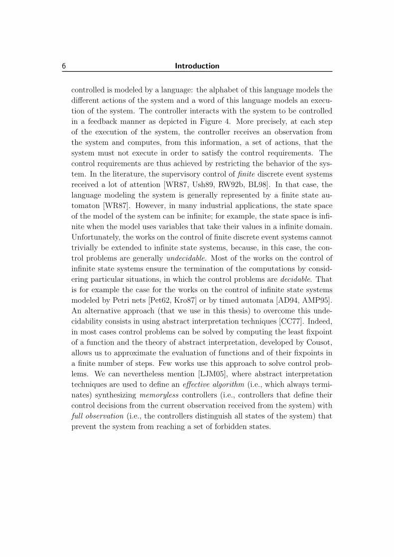
6 Introduction
controlled is modeled by a language: the alphabet of this language models the
different actions of the system and a word of this language models an execu-
tion of the system. The controller interacts with the system to be controlled
in a feedback manner as depicted in Figure 4. More precisely, at each step
of the execution of the system, the controller receives an observation from
the system and computes, from this information, a set of actions, that the
system must not execute in order to satisfy the control requirements. The
control requirements are thus achieved by restricting the behavior of the sys-
tem. In the literature, the supervisory control of finite discrete event systems
received a lot of attention [WR87, Ush89, RW92b, BL98]. In that case, the
language modeling the system is generally represented by a finite state au-
tomaton [WR87]. However, in many industrial applications, the state space
of the model of the system can be infinite; for example, the state space is infi-
nite when the model uses variables that take their values in a infinite domain.
Unfortunately, the works on the control of finite discrete event systems cannot
trivially be extended to infinite state systems, because, in this case, the con-
trol problems are generally undecidable. Most of the works on the control of
infinite state systems ensure the termination of the computations by consid-
ering particular situations, in which the control problems are decidable. That
is for example the case for the works on the control of infinite state systems
modeled by Petri nets [Pet62, Kro87] or by timed automata [AD94, AMP95].
An alternative approach (that we use in this thesis) to overcome this unde-
cidability consists in using abstract interpretation techniques [CC77]. Indeed,
in most cases control problems can be solved by computing the least fixpoint
of a function and the theory of abstract interpretation, developed by Cousot,
allows us to approximate the evaluation of functions and of their fixpoints in
a finite number of steps. Few works use this approach to solve control prob-
lems. We can nevertheless mention [LJM05], where abstract interpretation
techniques are used to define an effective algorithm (i.e., which always termi-
nates) synthesizing memoryless controllers (i.e., controllers that define their
control decisions from the current observation received from the system) with
full observation (i.e., the controllers distinguish all states of the system) that
prevent the system from reaching a set of forbidden states.

Introduction 7
Objectives and Structure of this Thesis
In this thesis, we want to develop control methods based on the supervisory
control theory. In this theory, most of the works suppose that the system to be
controlled has a finite state space. However, when modeling realistic systems,
it is often convenient to manipulate state variables instead of simply atomic
states, allowing a compact way to specify systems handling data. In that case,
to provide a homogeneous treatment of these models, it is convenient to consider
variables, whose domain is infinite, and thus systems with an infinite state space.
Unfortunately, works on the control of finite state systems cannot trivially be
extended to infinite state systems for undecidability reasons. Moreover, it is
more interesting to consider the synthesis of controllers with partial observation.
Indeed, controllers interact with the plant through sensors and actuators and,
in general, they have only a partial observation of the system, because these
materials have not an absolute precision or because some parts of the system are
not observed by the controllers.
Therefore, in this thesis, we are interested in the control of infinite state
systems with partial observation. This problem is generally undecidable and to
overcome this negative result, we use, as in [LJM05], abstract interpretation tech-
niques which ensure that our algorithm always terminate. Moreover, we want
to provide the most complete contribution it is possible to bring to this topic.
Hence, we consider more and more realistic problems. More precisely, we start
our work by considering a centralized framework (i.e., the system is controlled by
a single controller) and by synthesizing memoryless controllers (i.e., controllers
that define their control policy from the current observation received from the
system). Next, to obtain better solutions, we consider the synthesis of controllers
that record a part or the whole of the execution of the system and use this in-
formation to define the control policy. However, in some cases, the nature of the
system to be controlled makes unrealistic the use of a centralized framework; for
example, in the case of distributed systems. We then consider, more elaborate
frameworks, which allow us to control this kind of systems. We first work on
a decentralized framework which is useful for the control of distributed systems
with synchronous communications. In this framework, the system is controlled
by several controllers, that are coordinated to jointly ensure the desired prop-
erties. After, we consider a modular framework, which actually corresponds to
a decentralized framework where the structure of the system to be controlled
is exploited to perform the computations more efficiently. Unfortunately, these

8 Introduction
frameworks cannot be used for the control of an interesting and more complex
class of distributed systems: the distributed systems with asynchronous com-
munications. Therefore, we define a distributed framework which allows us to
control this kind of systems.
This thesis is structured as follows.
Chapter 1 - Preliminaries. In this chapter, we briefly present fundamental
concepts and existing results that we will use throughout this thesis.
Chapter 2 - Supervisory Control of Discrete Event Systems. In this
chapter, we present a state of the art on supervisory control theory of finite
discrete event systems and of infinite state systems.
Chapter 3 - Synthesis of Centralized Memoryless Controllers with Par-
tial Observation for Infinite State Systems. In chapter 3, we are interested
in the state avoidance control problem for infinite state systems. This problem
consists in synthesizing a controller that prevents the system from reaching a
set of forbidden states. In our framework, we model infinite state systems by
symbolic transition systems [HMR05]. This formalism allows us to compactly
manipulate infinite state systems. Moreover, we place ourself in the context of
controllers that are memoryless and that do not perfectly observe the system to
be controlled. This assumption of partial observation makes the problem harder,
but also more realistic, because the sensors, that the controllers use to observe
the system, have generally neither an absolute precision, nor a full observation
of the system. We provide algorithms, which synthesize controllers with partial
observation for the state avoidance control problem for both cases where the
deadlock free property must and must not be ensured. Since the problems, that
we want to solve, are undecidable, we use, as in [LJM05], abstract interpretation
techniques to obtain effective algorithms at the price, however, of some approxi-
mations in the solutions that we compute. The content of this chapter is based
on the followings article:
G. Kalyon, T. Le Gall, H. Marchand, T. Massart. Control of Infinite Symbolic
Transition Systems under Partial Observation. In European Control Confer-
ence (ECC’09), pages 1456-1462, Budapest, Hungary, August 2009.
Chapter 4 - Synthesis of Centralized k-memory and Online Controllers
with Partial Observation for Infinite State Systems. In this chapter,

Introduction 9
we extend the previous work by synthesizing k-memory controllers and online
controllers. A k-memory controller uses the last k observations received from the
system to define its control decisions and an online controller computes, during
the execution of the system, an estimate of the current state of the system that
it uses to define its control policy. We also compare the control quality of our
memoryless, k-memory, and online controllers. The content of this chapter is
based on the following article:
G. Kalyon, T. Le Gall, H. Marchand and T. Massart. Symbolic Supervi-
sory Control of Infinite Transition Systems under Partial Observation using
Abstract Interpretation. Submitted to Journal of Discrete Event Dynamical
Systems.
Chapter 5 - Synthesis of Decentralized and Modular Controllers for
Infinite State Systems. In this chapter, we provide algorithms computing
decentralized controllers for infinite state systems. In a decentralized framework,
the system is controlled by n controllers, that are coordinated to jointly ensure
the desired properties. This framework is useful for the control of more complex
systems like the distributed systems with synchronous communications. We con-
sider the state avoidance control problem for both cases where the deadlock free
property must and must not be ensured. Again, we use abstract interpretation
techniques to ensure the termination of the computations, since these problems
are undecidable. However, in this framework, we have no information regarding
the structure of the distributed system to be controlled while the computation
of the controllers, which implies that these computations are performed on the
model of the global system. We then adapt this approach to the case where
the structure of the distributed system to be controlled is known. We explain
how this structure can be exploited to perform most of the computations locally
i.e., on each subsystem which composes the global system to be controlled. The
content of this chapter is based on the following articles:
G. Kalyon, T. Le Gall, H. Marchand, and T. Massart. Controle Decentralise de
Systemes Symboliques Infinis sous Observation Partielle. Journal Europeen
des Systemes Automatises (7eme Colloque Francophone sur la Modelisation
des Systemes Reactifs), 43/7-9-2009:805-819, 2009.
G. Kalyon, T. Le Gall , H. Marchand and T. Massart. Decentralized Control
of Infinite State Systems. Submitted to Journal of Discrete Event Dynamical
Systems.
10 Introduction
Chapter 6 - Distributed Supervisory Control of FIFO Systems. In chap-
ter 6, we consider the state avoidance control problem in a distributed framework.
In this context, the system to be controlled is defined by n subsystems communi-
cating asynchronously through reliable unbounded FIFO channels. Each subsys-
tem is modeled by a communicating finite state machine [BZ83a] and the state
space of the global system can be infinite, because the queue are unbounded. We
define an algorithm which computes n local controllers (each local controller con-
trols a subsystem) that prevent the global system from reaching a set of forbidden
states. The controllers, that we define, can exchange, during the execution of the
system, information through reliable unbounded FIFO channels. They exploit
this information to compute an estimate of the current state of the system that
they use to define their control policy. Once again, since the problem, that we
consider, is undecidable, we use abstract interpretation techniques to ensure the
termination of the computations. The content of this chapter is based on the
following technical report:
B. Jeannet, G. Kalyon, T. Le Gall, H. Marchand and T. Massart. Distributed
Supervisory Control of FIFO Systems. Technical report, ULB, 2010.
Chapter 7 - Computational Complexity of the Synthesis of Memory-
less Controllers with Partial Observation for Finite State Systems. In
this chapter, we restrict our attention to the case, where the system to be con-
trolled has a finite state space, and we study the time complexity of some control
problems related to the state avoidance control problem. In particular, we show
that the problem, which consists in computing a maximal solution for the state
avoidance control problem, cannot be solved in polynomial time unless P = NP.
The content of this chapter is based on the following article:
G. Kalyon, T. Le Gall, H. Marchand, and T. Massart. Computational Com-
plexity for State-feedback Controllers with Partial Observation. In 7th Inter-
national Conference on Control and Automation (ICCA’09), pages 436-441,
Christchurch, New Zealand, December 2009.
Appendix A - Smacs (Symbolic MAsked Controller Synthesis). In
this chapter, we describe our tool SMACS which implements some control
algorithms defined in this thesis. This tool allows us to experimentally evaluate
our approach based on the use of abstract interpretation to obtain effective
algorithms.

Introduction 11
Finally, we conclude this thesis by summarizing our work and by suggesting
future works.

12 Introduction

Part I
Fundamentals and Definitions
13


Chapter
1Preliminaries
In this chapter, we recall the key concepts used throughout this thesis.
First, in section 1.1, we present some basic notions on sets, functions,
predicates,... Next, in section 1.2, we briefly recall the concepts of
languages and of automata. In section 1.3, we give a short introduction to lattice
theory. Finally, in section 1.4, we briefly present the abstract interpretation
framework. Abstract interpretation will be widely used in this thesis to obtain
effective control algorithms (i.e., control algorithms which always terminate) for
infinite state systems.
1.1 Basic Notions
In this section, we recall some basic notions and notations that will be used
throughout this thesis.
Sets. N denotes the set of natural numbers {1, 2, . . .} and N0 denotes the set
{0, 1, 2, . . .}. The set of integer numbers {0, 1, 2, . . .} ∪ {−1,−2, . . .} is denoted
by Z. The set of rational (resp. real) numbers is denoted by Q (resp. R). Bdenotes the set of boolean values {tt, ff}, where tt (resp. ff) stands for true (resp.
false). Given two numbers a, b ∈ Z ∪ {−∞,∞}, the interval between a and b
is denoted by [a, b] and is defined by [a, b]def= {x ∈ Z ∪ {−∞,∞} | a ≤ x ≤ b}.
Given a set X, 2X denotes the power set of X i.e., the set of all subsets of X,
16 Chapter 1
and |X| ∈ N0 ∪ {∞} denotes the cardinality of X i.e., the number of elements
in X. Given a set X and a subset Y ⊆ X, the complement of Y w.r.t. X
is denoted by Y c and is defined by Y c def= X \ Y . Given two sets X and Y ,
the cartesian product of X and Y is denoted by X × Y . Given a set X and a
number n ≥ 1, Xn denotes the cartesian product X × . . .×X︸ ︷︷ ︸n
, which gives the
set of n-tuples of elements of X. The empty set is denoted by ∅.
Coverings and Partitions. Given a set X, a covering C of X is a set
of non-empty subsets of X such that⋃
Y ∈C Y = X and a partition P of X
is a covering such that ∀Y, Z ∈ P : Y ∩ Z = ∅. To express that the sets
X1, X2, . . . , Xn constitute a partition P of X, we write X = X1 ]X2 ] . . .]Xn.
Tuples. Given an n-tuple ~a = 〈a1, . . . , an〉 and two numbers i, j ∈ [1, n]
with i ≤ j, ~a⌋
[i:j]denotes the tuple made of the components of ~a between
ai and aj i.e., ~a⌋
[i:j]
def= 〈ai, . . . , aj〉. When i = j, ~a
⌋[i:i]
is denoted by ~a⌋
[i].
This notation is extended to sets of n-tuples as expected: given a set ~X
of n-tuples, ~X⌋
[i:j]
def= {~x
⌋[i:j]| ~x ∈ ~X}. Given two n-tuples ~a1 and ~a2, the
concatenation of these two n-tuples is denoted by ~a1 ·∪~a2 and is defined by the
pair ~a1 ·∪~a2def= 〈~a1,~a2〉. The empty tuple is denoted by ∅.
Functions. A function f from a set X, called the domain, to a set Y , called
the codomain, is denoted by f : X → Y and is a relation between X and Y ,
which associates at most one element y ∈ Y with each element x ∈ X; this
element y is denoted by f(x). A function f : X → Y is total if, for each
x ∈ X, |f(x)| = 1; otherwise it is called partial. A function f : X → Y is
(i) injective if ∀x1, x2 ∈ X : (f(x1) = f(x2)) ⇒ (x1 = x2), (ii) surjective if
∀y ∈ Y,∃x ∈ X : f(x) = y, and (iii) bijective if it is injective and surjective.
Given a function f : X → Y and a set Z ⊆ X, f(Z) denotes⋃
z∈Z f(z).
Given a set X, IdX : X → X denotes the identity function, which is defined,
for each x ∈ X, by IdX(x)def= x. The preimage function of a function
f : X → Y is denoted by f−1 : Y → 2X and is defined, for each y ∈ Y ,
by f−1(y)def= {x ∈ X | f(x) = y}. The composition g ◦ f of two functions
f : X → Y and g : Y → Z is a function from the domain X to the codomain
Z and is defined, for each x ∈ X, by (g ◦ f)(x)def= g(f(x)). Given a function
f : X → X and a number n ∈ N0, the nth functional power of f is denoted by
fn and is recursively defined as follows: (i) f 0 def= IdX , and (ii) fn def
= fn−1 ◦ f ,
Preliminaries 17
if n ≥ 1. We sometimes use the Church’s notation [Chu36] where a function
f : X → Y is denoted by λx.f(x).
Predicates. Let X be a set, a predicate P : X → {tt, ff} over the set X is a
function, which associates a truth value belonging to {tt, ff} with each element
x ∈ X; this truth value is denoted by P (x). P (x) = tt and P (x) = ff are
respectively denoted by P (x) and ¬P (x). The predicate P : X → {tt, ff} can
also be viewed as a subset Y ⊆ X defined by Ydef= {x ∈ X |P (x)}. Given
a set X, TTX : X → {tt, ff} denotes the true predicate, which is defined, for
each x ∈ X, by TTX(x) = tt. Similarly, FFX : X → {tt, ff} denotes the false
predicate, which is defined, for each x ∈ X, by FFX(x) = ff.
Variables. The domain of a variable v is denoted by Dv, and the domain of
an n-tuple of variables V = 〈v1, . . . , vn〉 is denoted by DV and is defined by
DVdef=∏
i∈[1,n]Dvi. Throughout this thesis, we will frequently use ~ν to denote a
value 〈ν1, . . . , νn〉 ∈ DV .
Relations. A binary relation R ⊆ X ×X is (i) reflexive if ∀x ∈ X : 〈x, x〉 ∈ R,
(ii) symmetric if ∀x, y ∈ X : (〈x, y〉 ∈ R) ⇒ (〈y, x〉 ∈ R), (iii) antisymmetric
if ∀x, y ∈ X : ((〈x, y〉 ∈ R) ∧ (〈y, x〉 ∈ R)) ⇒ (x = y), and (iv) transitive if
∀x, y, z ∈ X : ((〈x, y〉 ∈ R) ∧ (〈y, z〉 ∈ R)) ⇒ (〈x, z〉 ∈ R). A partial order
is a reflexive, antisymmetric and transitive binary relation and an equivalence
relation is a reflexive, symmetric and transitive binary relation.
1.2 Languages and Automata
Definition of a Language. An alphabet Σ is a finite set of symbols called
letters. A word w over Σ is a sequence of letters of Σ; the empty word is denoted
by ε. The set of finite words over Σ is denoted by Σ∗ and a language over
Σ is defined as a subset L ⊆ Σ∗ of finite words. The key operation to build
words from an alphabet Σ is the concatenation: given two words w1, w2 ∈ Σ∗,
the concatenation of w1 and w2 is denoted by w1.w2 (or w1w2 for short) and is
defined by a new word composed of the letters of w1 immediately followed by the
letters of w2. Given a subset Σ′ ⊆ Σ, the projection of a word w ∈ Σ∗ on Σ′ is
obtained from w by keeping only the symbols of Σ′. This operation is formally

18 Chapter 1
defined by the function P : Σ∗ → Σ′∗, where, for each w ∈ Σ∗:
P (w)def=
ε if w = ε
P (w′).a if (w = w′.a) ∧ (a ∈ Σ′)
P (w′) if (w = w′.a) ∧ (a 6∈ Σ′)
(1.1)
The prefix-closure of a language L (over Σ) is a language denoted by L and
defined by all prefixes of all words of L i.e., L def= {w ∈ Σ∗ | ∃w′ ∈ Σ∗ : w.w′ ∈ L}.
Automata. An automaton is a well-known formalism which models languages
and which corresponds to a directed graph with actions (also called labels) on
the edges. This concept is formally defined as follows:
Definition 1.1 (Automaton)
An automaton T is defined by a 5-tuple 〈X,X0, Xm,Σ,∆〉, where1:
• X is a countable set of states
• X0 is the set of initial states
• Xm is a set of marked (or final or accepting) states
• Σ is a finite set of actions (or alphabet)
• ∆ ⊆ X × Σ×X is the transition relation
An automaton T = 〈X,X0, Xm,Σ,∆〉 is deterministic2 if (i) |X0| = 1 and (ii)
∀x1 ∈ X,∀σ ∈ Σ : [(〈x1, σ, x2〉 ∈ ∆) ∧ (〈x1, σ, x′2〉 ∈ ∆)]⇒ (x2 = x′2). Moreover,
T is finite if the set X of states is finite. A finite automaton can be transformed
into a finite deterministic automaton by using the subset construction [HMU06].
In the sequel, a transition 〈x1, σ, x2〉 ∈ ∆ is also denoted by x1σ−→ x2.
Example 1.1
Figure 1.1 shows a graphical representation of a finite automaton T =
〈X,X0, Xm,Σ,∆〉. In this diagram, states and transitions are respectively
represented by nodes and edges. The initial states are identified by a small
incoming arrow and the final states are doubly circle nodes. Thus, the au-
tomaton T represented by this diagram is defined as follows:
1In the sequel, when we will not need the set of marked states Xm, we will define anautomaton by a 4-tuple 〈X, X0,Σ,∆〉.
2In some references [ASU86], an equivalent definition is given: (i) |X0| = 1 and (ii) ∀x1 ∈X,∀σ ∈ Σ : |{〈x1, σ, x2〉 | 〈x1, σ, x2〉 ∈ ∆}| = 1.

Preliminaries 19
x1
x4
x2
x3
a
b c
d
Figure 1.1 - An example of finite deterministic automata.
• X = {x1, x2, x3, x4}
• X0 = {x1}
• Xm = {x4}
• Σ = {a, b, c, d}
• ∆ = {〈x1, a, x2〉, 〈x2, b, x3〉, 〈x2, d, x4〉, 〈x3, c, x3〉}
We now define some notions, related to automata, that are often used in the
control of discrete event systems. For convenience, we suppose that we work on
an automaton T = 〈X,X0, Xm,Σ,∆〉.
Generated and Marked Languages. There are mainly two languages which
are associated to an automaton: the generated and marked languages.
Definition 1.2 (Generated Language)
A finite word w = σ1.σ2 . . . σn is generated by an automaton T if there exists
a finite sequence of states x0, x1, . . . , xn ∈ X such that (i) x0 ∈ X0, and (ii)
∀i ∈ [0, n − 1] : 〈xi, σi+1, xi+1〉 ∈ ∆. The language L(T ) generated by T is
then defined by the set of finite words w generated by T .
The generated language thus describes the set of possible behaviors of an
automaton and is obviously prefix-closed.

20 Chapter 1
Definition 1.3 (Marked Language)
A finite word w = σ1.σ2 . . . σn is marked by an automaton T if there exists
a finite sequence of states x0, x1, . . . , xn ∈ X such that (i) x0 ∈ X0, (ii)
∀i ∈ [0, n − 1] : 〈xi, σi+1, xi+1〉 ∈ ∆ and (iii) xn ∈ Xm. The language Lm(T )
marked by T is then defined by the set of finite words w marked by T .
The marked language thus describes the set of possible behaviors of an
automaton which end in a final state. For example, if the final states correspond
to the states in which a task is accomplished, the marked language then
represents the set of behaviors corresponding to the achievement of a task.
Regular Languages. Regular languages form an interesting class of languages
defined as follows:
Definition 1.4 (Regular Language)
A language L is regular if it is marked by a finite automaton.
Further in this thesis, we will use this concept in the control of distributed
systems to abstract the content of the queues of these systems.
Reachable and Coreachable States. The concepts of reachable and coreach-
able states are defined in the following way for automata.
Definition 1.5 (Reachable State)
A state x′ is reachable from a state x in an automaton T if x′ can be reached
from x by a finite sequence of transitions i.e., there exist a finite sequence of
states x0, x1, . . . , xn ∈ X and a finite sequence of actions σ1, σ2, . . . , σn ∈ Σ
such that (i) x0 = x, (ii) xn = x′, and (iii) ∀i ∈ [0, n−1] : 〈xi, σi+1, xi+1〉 ∈ ∆.
A state x is reachable in the system T if it is reachable from an initial state of
T .
Definition 1.6 (Coreachable State)
A state x′ is coreachable from a state x in an automaton T if x can be reached
from x′ by a finite sequence of transitions i.e., there exist a finite sequence of
states x0, x1, . . . , xn ∈ X and a finite sequence of actions σ1, σ2, . . . , σn ∈ Σ
such that (i) x0 = x′, (ii) xn = x, and (iii) ∀i ∈ [0, n−1] : 〈xi, σi+1, xi+1〉 ∈ ∆.
Backward and Forward Operators. The backward and forward operators
Preliminaries 21
are defined in the following way:
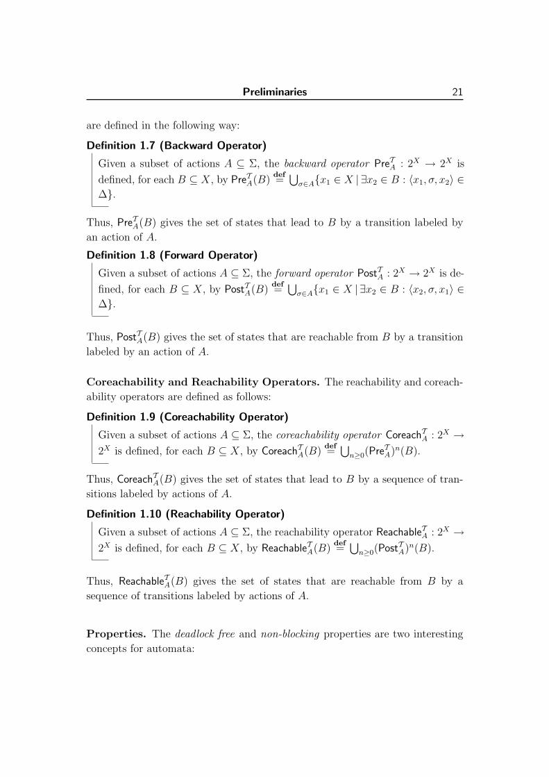
Definition 1.7 (Backward Operator)
Given a subset of actions A ⊆ Σ, the backward operator PreTA : 2X → 2X is
defined, for each B ⊆ X, by PreTA(B)def=⋃
σ∈A{x1 ∈ X | ∃x2 ∈ B : 〈x1, σ, x2〉 ∈∆}.
Thus, PreTA(B) gives the set of states that lead to B by a transition labeled by
an action of A.
Definition 1.8 (Forward Operator)
Given a subset of actions A ⊆ Σ, the forward operator PostTA : 2X → 2X is de-
fined, for each B ⊆ X, by PostTA(B)def=⋃
σ∈A{x1 ∈ X | ∃x2 ∈ B : 〈x2, σ, x1〉 ∈∆}.
Thus, PostTA(B) gives the set of states that are reachable from B by a transition
labeled by an action of A.
Coreachability and Reachability Operators. The reachability and coreach-
ability operators are defined as follows:
Definition 1.9 (Coreachability Operator)
Given a subset of actions A ⊆ Σ, the coreachability operator CoreachTA : 2X →2X is defined, for each B ⊆ X, by CoreachTA(B)
def=⋃
n≥0(PreTA)n(B).
Thus, CoreachTA(B) gives the set of states that lead to B by a sequence of tran-
sitions labeled by actions of A.
Definition 1.10 (Reachability Operator)
Given a subset of actions A ⊆ Σ, the reachability operator ReachableTA : 2X →2X is defined, for each B ⊆ X, by ReachableTA(B)
def=⋃
n≥0(PostTA)n(B).
Thus, ReachableTA(B) gives the set of states that are reachable from B by a
sequence of transitions labeled by actions of A.
Properties. The deadlock free and non-blocking properties are two interesting
concepts for automata:

22 Chapter 1
Definition 1.11 (Deadlock Free Property)
A state x1 ∈ X is deadlock free if ∃σ ∈ Σ,∃x2 ∈ X : 〈x1, σ, x2〉 ∈ ∆, and an
automaton T is deadlock free if all states, that are reachable in this automaton,
are deadlock free.
This property means that it is always possible to fire at least one action from
any reachable state.
Definition 1.12 (Non-blocking Property)
A state x ∈ X is non-blocking if (ReachableTΣ(x)) ∩ Xm 6= ∅. An automaton
T is non-blocking if all states, that are reachable in this automaton, are non-
blocking; in this case, Lm(T ) = L(T ).
This property means that a marked state can always be reached from any reach-
able state. Notice that a non-blocking automaton can have deadlocking marked
states.
1.3 Lattice Theory
In this section, we recall some basic notions on lattice theory. First, in sec-
tion 1.3.1, we introduce the concepts of partial orders and of lattices, and next,
in section 1.3.2, we turn our attention to fixpoint computations.
1.3.1 Partially Ordered Set and Lattice
The notion of partially ordered set is defined as follows:
Definition 1.13 (Partially Ordered Set)
Let X be a set and v⊆ X × X be a binary relation. The pair 〈X,v〉 is a
partially ordered set if v is a partial order on X.
For example, 〈N0,≤〉 and 〈Z,≤〉 are partially ordered sets.
Let Y ⊆ X be a subset of X and v⊆ X ×X be a partial order. An element
x ∈ X is an upper bound (resp. lower bound) of Y if ∀y ∈ Y : y v x (resp.
x v y). Moreover, x is the least upper bound of Y (i) if it is an upper bound of
Y , and (ii) if x v y, for every upper bound y of Y . Similarly, x is the greatest
lower bound of Y (i) if it is a lower bound of Y , and (ii) if y v x, for every lower
bound y of Y . The least upper bound and the greatest lower bound of a set Y do

Preliminaries 23
not always exist. When they exist, they are unique (since v is antisymmetric)
and they are respectively denoted by⊔Y and
dY . The operator
⊔(resp.
d) is
also called the join operator (resp. meet operator) and⊔{x, y} (resp.
d{x, y})
is written x t y (resp. x u y).The notion of lattice is defined as follows:
Definition 1.14 (Lattice)
Let X be a set and v⊆ X ×X be a partial order. The pair 〈X,v〉 is a lattice
if, for any x, y ∈ X, the least upper bound and the greatest lower bound of
the set {x, y} are defined.
Definition 1.15 (Complete Lattice)
Let X be a set and v⊆ X × X be a partial order. The element 〈X,v,⊔,d,>,⊥〉 is a complete lattice if every non-empty subset Y ⊆ X has a
least upper bound⊔Y and a greatest lower bound
dY . In particular, a com-
plete lattice admits a v-maximal element (also called top) > =⊔X and a
v-minimal element (also called bottom) ⊥ =dX.
Example 1.2
Let X be a set. The power set lattice PSL(X) = 〈2X ,⊆,∪,∩, X, ∅〉 is a com-
plete lattice, which has (i) the union as least upper bound, (ii) the intersection
as greatest lower bound, (iii) the set X as ⊆-maximal element, and (iv) the
set ∅ as ⊆-minimal element.
1.3.2 Fixpoints
Given a set X and a function f : X → X over the lattice 〈X,v〉, an element
x ∈ X is a fixpoint of f if x = f(x). We define FP(f)def= {x ∈ X | f(x) = x}. The
least fixpoint of f (denoted by lfpv(f)) is the greatest lower bound of FP(f) i.e.,
lfpv(f)def=
d(FP(f)). Similarly, the greatest fixpoint of f (denoted by gfpv(f))
is the least upper bound of FP(f) i.e., gfpv(f)def=⊔
(FP(f)). An element x ∈ Xis a post-fixpoint (resp. pre-fixpoint) if x w f(x) (resp. x v f(x)).
We present two well-known theorems on fixpoints. But before that, we define
the concepts of monotonic and continuous functions.
24 Chapter 1
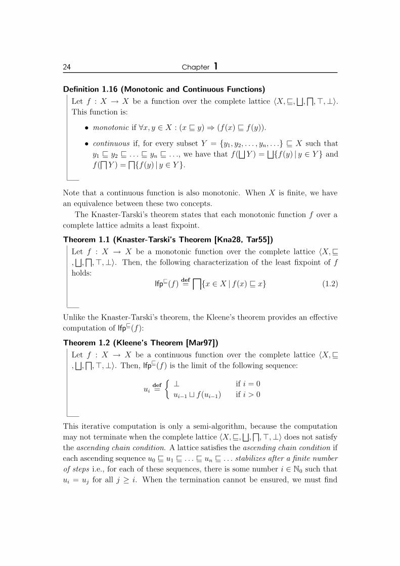
Definition 1.16 (Monotonic and Continuous Functions)
Let f : X → X be a function over the complete lattice 〈X,v,⊔,d,>,⊥〉.
This function is:
• monotonic if ∀x, y ∈ X : (x v y)⇒ (f(x) v f(y)).
• continuous if, for every subset Y = {y1, y2, . . . , yn, . . .} v X such that
y1 v y2 v . . . v yn v . . ., we have that f(⊔Y ) =
⊔{f(y) | y ∈ Y } and
f(dY ) =
d{f(y) | y ∈ Y }.
Note that a continuous function is also monotonic. When X is finite, we have
an equivalence between these two concepts.
The Knaster-Tarski’s theorem states that each monotonic function f over a
complete lattice admits a least fixpoint.
Theorem 1.1 (Knaster-Tarski’s Theorem [Kna28, Tar55])
Let f : X → X be a monotonic function over the complete lattice 〈X,v,⊔,d,>,⊥〉. Then, the following characterization of the least fixpoint of f
holds:
lfpv(f)def=
l{x ∈ X | f(x) v x} (1.2)
Unlike the Knaster-Tarski’s theorem, the Kleene’s theorem provides an effective
computation of lfpv(f):
Theorem 1.2 (Kleene’s Theorem [Mar97])
Let f : X → X be a continuous function over the complete lattice 〈X,v,⊔,d,>,⊥〉. Then, lfpv(f) is the limit of the following sequence:
uidef=
{⊥ if i = 0
ui−1 t f(ui−1) if i > 0
This iterative computation is only a semi-algorithm, because the computation
may not terminate when the complete lattice 〈X,v,⊔,d,>,⊥〉 does not satisfy
the ascending chain condition. A lattice satisfies the ascending chain condition if
each ascending sequence u0 v u1 v . . . v un v . . . stabilizes after a finite number
of steps i.e., for each of these sequences, there is some number i ∈ N0 such that
ui = uj for all j ≥ i. When the termination cannot be ensured, we must find

Preliminaries 25
a way to overapproximate lfpv(f). For that, we may use abstract interpretation
techniques (see section 1.4), which allow us to compute a sequence which always
stabilizes after a finite number of steps.
One can note that results similar to Theorems 1.1 and 1.2 exist for gfpv(f).
1.4 Abstract Interpretation
In general, verification problems can be solved by computing the least (or great-
est) fixpoint of some functions; the computation of the set of reachable states
in a system is a classical example. By the Kleene’s theorem, these fixpoints
can be solved by an iterative algorithm i.e., successive values of the solution are
computed until stabilization. Unfortunately, for many interesting lattices, this
algorithm may not terminate, because the number of iterations can be infinite
or too big to allow an efficient analysis. Abstract interpretation allows us to
compute an overapproximation of these fixpoints. For that, it substitutes the
computations in the concrete lattice by computations in a simpler abstract lat-
tice. Moreover, to ensure the termination of the computations, it provides a
powerful tool, the widening operator, which attempts to find an invariant in a
finite number of iterations.
In the remaining part of this section, we present the general framework of ab-
stract interpretation, the Galois connection framework, where the concrete and
abstract lattices are supposed to be complete. Next, we present the representa-
tion framework, which can be used when the abstract lattice is not complete; we
will use this framework in this thesis.
1.4.1 The Galois Connection Framework
The Galois connection framework is the general framework of abstract inter-
pretation and it is based on two key concepts: the Galois connection and the
widening operator [CC77].
Galois Connection. The concrete lattice 〈X,v〉 is substituted by an abstract
lattice 〈Λ,v]〉 (the abstract lattice can be seen as a simplification of the concrete
lattice, which allows us to describe some particular subsets of the state space
only). Both lattices must be complete and they are linked by a Galois connection
〈α, γ〉, where the monotonic abstraction function α : X → Λ and the monotonic

26 Chapter 1
concretization function γ : Λ→ X satisfy the following property [CC77]:
∀x ∈ X,∀` ∈ Λ : α(x) v] `⇔ x v γ(`) (1.3)
The abstraction function can be seen as a function which attempts to approximate
the sets of concrete states and the concretization function can be seen as a
function which gives a meaning to these approximate sets.
The Galois connection between the complete lattices 〈X,v〉 and 〈Λ,v]〉 is
generally denoted by 〈X,v〉 −−→←−−αγ〈Λ,v]〉 and ensures the computation of an
overapproximation of the least fixpoint lfpv(f) of a function f . Indeed, instead
of computing the least fixpoint of the function f (concrete lattice), we compute
the least fixpoint of the function f ] def= α ◦ f ◦ γ, which always satisfies the
following property: lfpv(f) v γ(lfpv]
(f ])). Thus, the concretization of the least
fixpoint lfpv]
(f ]) gives an overapproximation of lfpv(f).
Example 1.3
Let us consider the power set lattice PSL(Z) = 〈2Z,⊆,∪,∩,Z,⊥〉 and the
lattice of intervals 〈I,v,⊔,d,>,⊥〉, where (i) I = {[a, b] | (a ∈ Z∪{−∞})∧
(b ∈ Z ∪ {∞}) ∧ (a ≤ b)} ∪ {∅}, (ii) v,⊔,d
are respectively the classical
inclusion, union and intersection on intervals, (iii) > = [−∞,∞], and (iv)
⊥ = ∅. Both lattices are complete and they can be linked by the following
Galois connection 〈2Z,⊆〉 −−→←−−αγ〈I,v〉, where (i) the concretization function
γ : I → 2Z is defined, for each I ∈ I, by γ(I) = {i | i ∈ I}, and (ii) the
abstraction function α : 2Z → I is defined, for each Z ∈ 2Z, by:
α(Z) =
{⊥ if Z = ∅[min(Z),max(Z)] otherwise
Widening Operator. When the abstract lattice does not satisfy the ascending
chain condition, the computation of lfpv]
(f ]) may not terminate. To ensure the
feasibility of this fixpoint computation, we can use a widening operator ∇, which
tries to guess the limit of an ascending sequence of elements of a lattice in a
finite number of steps [CC77]. This concept is formally defined as follows:
Definition 1.17 (Widening Operator)
Let 〈Λ,v],⊔,d,>,⊥〉 be a lattice. ∇ : Λ× Λ→ Λ is a widening operator if:
• ∀x, y ∈ Λ : (x v] x∇y) ∧ (y v] x∇y) (or equivalently x t y v] x∇y).

Preliminaries 27
• for each ascending sequence x0 v] x1 v] . . . v] xn v] . . ., the ascending
sequence (yi)i∈N0 , defined as follows, stabilizes after a finite number of
steps:
yidef=
{x0 if i = 0
yi−1∇xi if i > 0
The first condition ensures that the widening operator is an overapproximation
of the least upper bound and the second one ensures the termination of the
computation of the fixpoints.
Example 1.4
A classical widening operator ∇ for the lattice of intervals 〈I,v,⊔,d,>,⊥〉
is defined, for each [`1, r1], [`2, r2] ∈ I, by [`1, r1]∇[`2, r2]def= [`, r], where:
` =
{`1 if `2 ≥ `1−∞ otherwise
r =
{r1 if r1 ≥ r2∞ otherwise
We can iteratively compute an overapproximation of the least fixpoint of a
function by using the widening operator ∇ as follows:
Theorem 1.3 ([CC77])
Let f ] : Λ → Λ be a function over the complete abstract lattice 〈Λ,v]
,⊔,d,>,⊥〉. The sequence (ui)i∈N0 defined by:
uidef=
⊥ if i = 0
ui−1 if (i > 0) ∧ (f ](ui−1) v] ui−1)
ui−1∇f ](ui−1) otherwise
stabilizes after a finite number of steps and its limit u∞ is such that lfpv]
(f ]) v]
u∞.
Example 1.5
Let us consider the following part of a C++ program where x is an integer
variable and Ci (∀i ∈ [0, 3]) is a control point which represents the possible
values of the variable x after the execution of the instruction which follows
this control point. We want to compute the values of C0, C1, C2 and C3:

28 Chapter 1
C0: int x;
C1: x = 0;
C2: while(x >= 0)
{
C3: x = x + 1;
}
The semantics of this program is defined by the following equation which gives
the value of each control point:C0 = >C1 = 0
C2 = (C1 ∪ C3) ∩ [0,∞[
C3 = incr(C2)
where > represents the entire state space and incr is a function which incre-
ments its parameter by one unit. To obtain the values of C0, C1, C2 and C3, we
define the function f(C0, C1, C2, C3) by 〈>, 0, (C1 ∪ C3) ∩ [0,∞[, incr(C2)〉and we compute its least fixpoint. This computation is performed in the
lattice of intervals 〈I,v,⊔,d,>,⊥〉 by using Theorem 1.3. We then ob-
tain the following sequence of values: (i) u0 = 〈⊥,⊥,⊥,⊥〉, (ii) u1 =
〈[>, [0, 0],⊥,⊥〉, (iii) u2 = 〈[>, [0, 0], [0, 0],⊥〉, (iv) u3 = 〈[>, [0, 0], [0, 0], [1, 1]〉,(v) u4 = 〈[>, [0, 0], [0, 0]∇[0, 1], [1, 1]〉 = 〈[>, [0, 0], [0,∞], [1, 1]〉, (vi) u5 =
〈[>, [0, 0], [0,∞], [1,∞]〉. Theorem 1.3 ensures that u5 is a post-fixpoint of
f and we remark that it is also the least fixpoint of this function.
1.4.2 The Representation Framework
The Galois connection framework supposes that the abstract and concrete lat-
tices are complete. However, many interesting abstract lattices, like the lattice
of convex polyhedra or the lattice of regular languages (that we will use in this
thesis) are not complete and cannot thus be used as abstract lattice in the Ga-
lois connection framework. To overcome this obstacle, an alternative framework,
called the representation framework, has been developed in [Bou92]. This frame-
work proceeds quite similarly to the Galois connection framework to formalize
the abstractions and to compute a safe overapproximation of the least fixpoint
of a function. The main difference concerns the assumptions imposed on the ele-

Preliminaries 29
ments used to formalize the abstractions, which are weaker in the representation
framework. In particular, the abstract lattice must only be a partially ordered
set.
More precisely, the concrete lattice and the abstract lattice are linked by a
representation [Bou92], which ensures the computation of an overapproximation
of the least fixpoint of a function in a finite number of steps:
Definition 1.18 (Representation [Bou92])
Let 〈X,v,⊔,d,>,⊥〉 be a complete lattice, 〈〈Λ,v],
⊔],d],>],⊥]〉, γ,∇〉 is
a representation of X if:
• 〈Λ,v],⊔],
d],>],⊥]〉 is a partially ordered set.
• γ : Λ → X is a monotonic concretization function, which associates a
concrete element with each abstract element. This function thus gives a
meaning to the abstract elements.
• ∇ is a widening operator, which satisfies the following constraint:
∀`1, `2 ∈ Λ : γ(`2) v] γ(`1∇`2). This widening operator ensures that
the computation of an overapproximation of the least fixpoint of a func-
tion always terminates.
To correctly perform the computations in the abstract lattice, there must exist
an abstraction function α : X → Λ which safely represents each element x ∈ Xby an element α(x) ∈ Λ i.e., γ(α(x)) w x. Thus, α can be seen as a function,
which approximates the elements of the concrete lattice.
In a sense, the concept of representation replaces the concepts of Galois con-
nection and of widening by imposing weaker conditions on the elements used to
formalize the abstractions.
We can iteratively compute an overapproximation of the least fixpoint of a
function by using the concept of representation as follows:
Theorem 1.4 ([Bou92])
Let 〈X,v〉 be a complete concrete lattice, 〈〈Λ,v],⊥〉, γ,∇〉 be a representation
of X, and f : X → X, f ] : Λ→ Λ be monotonic functions such that γ ◦ f ] wf ◦ γ, the sequence (ai)i∈N0 (where ∀i ∈ N0 : ai ∈ Λ) defined by:

30 Chapter 1
aidef=
{⊥ if i = 0
ai−1∇f ](ai−1) if i > 0
has a greatest element a∞, which is obtained after a finite number of steps and
which is a post-fixpoint of f ]. Moreover, γ(a∞) is a post-fixpoint of f .
An example illustrating this theory is given in section 3.4.2.
Chapter
2Supervisory Control of Discrete
Event Systems
In this chapter, we present a state of the art on supervisory control the-
ory of discrete event systems (DES for short) and introduce the main
problems, related to this domain, that we will study in this thesis. A
discrete event system is a system whose state space is given by a discrete set and
whose state transition mechanism is event-driven i.e., its state evolution depends
only on the occurrence of discrete events over the time. Supervisory control of
discrete event systems consists in imposing a given specification on a system by
means of a supervisor (also called controller) which runs in parallel with the
original system and which restricts its behavior.
The remainder of this chapter is structured as follows. In section 2.1, we
present a state of the art on supervisory control theory of finite discrete event
systems. The control of infinite state systems also received attention in the
literature and we present, in section 2.2, some results on the control of Petri nets,
timed automata, and systems with variables. In this chapter, we only focus on
supervisory control theory, except for the works on the control of timed automata
(see section 2.2.2), which are generally based on game theory.
32 Chapter 2
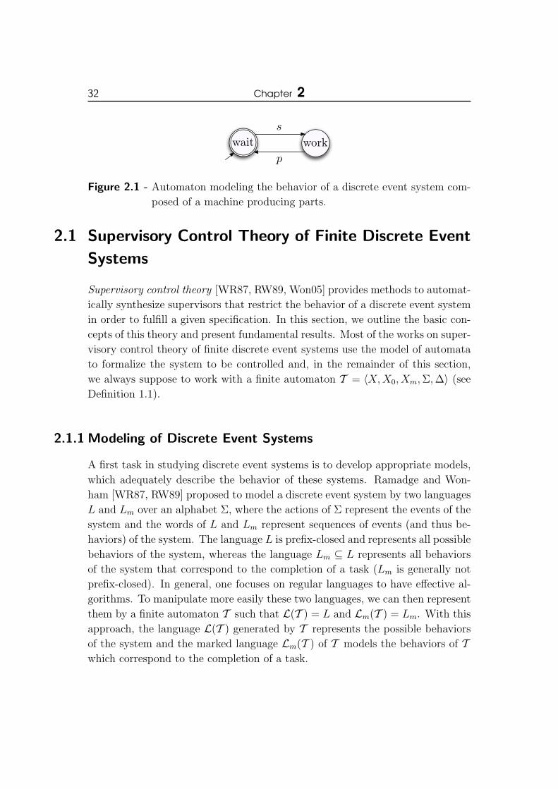
wait works
p
Figure 2.1 - Automaton modeling the behavior of a discrete event system com-
posed of a machine producing parts.
2.1 Supervisory Control Theory of Finite Discrete Event
Systems
Supervisory control theory [WR87, RW89, Won05] provides methods to automat-
ically synthesize supervisors that restrict the behavior of a discrete event system
in order to fulfill a given specification. In this section, we outline the basic con-
cepts of this theory and present fundamental results. Most of the works on super-
visory control theory of finite discrete event systems use the model of automata
to formalize the system to be controlled and, in the remainder of this section,
we always suppose to work with a finite automaton T = 〈X,X0, Xm,Σ,∆〉 (see
Definition 1.1).
2.1.1 Modeling of Discrete Event Systems
A first task in studying discrete event systems is to develop appropriate models,
which adequately describe the behavior of these systems. Ramadge and Won-
ham [WR87, RW89] proposed to model a discrete event system by two languages
L and Lm over an alphabet Σ, where the actions of Σ represent the events of the
system and the words of L and Lm represent sequences of events (and thus be-
haviors) of the system. The language L is prefix-closed and represents all possible
behaviors of the system, whereas the language Lm ⊆ L represents all behaviors
of the system that correspond to the completion of a task (Lm is generally not
prefix-closed). In general, one focuses on regular languages to have effective al-
gorithms. To manipulate more easily these two languages, we can then represent
them by a finite automaton T such that L(T ) = L and Lm(T ) = Lm. With this
approach, the language L(T ) generated by T represents the possible behaviors
of the system and the marked language Lm(T ) of T models the behaviors of Twhich correspond to the completion of a task.

Supervisory Control of Discrete Event Systems 33
Example 2.1
Let us consider a discrete event system composed of a machine producing parts.
This machine can start to work in order to produce a part (action s) and can
make a pause when the production of this part is finished (action p). This
system can be modeled by the language L = {ε, s, sp, sps, spsp, spsps, . . .}describing all possible behaviors of the system and by the language Lm =
{ε, sp, spsp, . . .} describing the completion of tasks. The automaton T repre-
senting these two languages is depicted in Figure 2.1, where wait is the only
initial and marked state.
In supervisory control theory, there are mainly two approaches to control a
system: the event-based approach and the state-based approach. Roughly, in the
event-based approach, the controller observes the actions fired by the system,
whereas, in the state-based approach, it observes the states of the system. These
two methods are detailed below.
2.1.2 Event-based Approach
The event-based approach [WR87, CL08] has been widely studied in the
literature; we present some important results and refer the reader to [CL08] for
further details.
Supervisory Control under Full Observation. The discrete event system
to be controlled is modeled by a finite automaton T ; its behavior may violate
some control objectives modeled by a language K ⊆ Lm(T ) (K is generally
not prefix-closed). The aim is to restrict the behavior of this system to satisfy
these objectives. For that, a particular device, called supervisor (or controller),
is designed to interact with the system. This supervisor S can be seen as a
function which, from the sequence of actions executed by the system, defines a
set of actions that must be forbidden to prevent the system from violating the
control objectives. However, the supervisor is not able to control some actions.
Indeed, the set of actions Σ is partitioned into the subset of controllable actions
Σc and the subset of uncontrollable actions Σuc. The uncontrollable actions,
which model for example failures, data from sensors or clock ticks, cannot be
forbidden by the supervisor.
More precisely, a supervisor is a function S : L(T ) → 2Σc which interacts
with the system T in a feedback manner as illustrated in Figure 2.2: after a

34 Chapter 2
T
S
w ∈ L(T )S(w) ⊆ Σc
System
Supervisor
Figure 2.2 - Feedback interaction between the system T to be controlled and the
supervisor S in an event-based approach under full observation.
sequence w of actions executed by the system, the supervisor computes a set
S(w) of controllable actions that the system must not execute. The closed loop
system T/S resulting from this interaction is called the controlled system and must
satisfy the control objectives. The generated language L(T/S) of this system is
recursively defined as the smallest set which satisfies the following conditions:
• ε ∈ L(T/S)
• ∀w ∈ L(T ),∀σ ∈ Σ : [(w ∈ L(T/S)) ∧ (wσ ∈ L(T )) ∧ (σ 6∈ S(w))] ⇔ (wσ ∈L(T/S))
In other words, a sequence wσ is a behavior of the controlled system if and only
if (i) w is a behavior of the controlled system, (ii) wσ is a possible behavior of
the system T , and (iii) the supervisor S allows the system to fire σ after the
sequence w.
The marked language Lm(T/S) of the controlled system is defined by
Lm(T/S)def= L(T/S)∩Lm(T ). A supervisor S is non-blocking if its corresponding
controlled system T/S is non-blocking i.e., Lm(T/S) = L(T/S).
A fundamental result for the supervisory control in the presence of uncon-
trollable actions is given by the following proposition:
Proposition 2.1 ([WR87])
Let T be the system to be controlled, and K ⊆ Lm(T ) (where K 6= ∅) be
the control objective, there exists a non-blocking supervisor S such that (i)
Lm(T/S) = K and (ii) L(T/S) = K if and only if:
• K is Lm(T )-closed i.e., K = K ∩ Lm(T ), and
• K is controllable w.r.t. Σuc and L(T ) i.e., KΣuc ∩ L(T ) ⊆ K.

Supervisory Control of Discrete Event Systems 35
x1
x3x2
a c
b
d
Figure 2.3 - Illustration of the controllability condition.
Moreover, if the controllability and Lm(T )-closure conditions are satisfied, a
supervisor S, which satisfies the specification, is defined as follows: for each
w ∈ L(T ),S(w)def= {σ ∈ Σc |wσ 6∈ K}.
Thus, a controlled system, which exactly achieves the specification, can be com-
puted if and only if the controllability and Lm(T )-closure conditions hold. The
first property means that if a behavior of K is extended with an uncontrollable
action and gives a behavior of L(T ), then this behavior must be included in K.
Consequently, firing an uncontrollable action always gives a good behavior. The
second condition ensures that the controlled system satisfies the non-blocking
property. The time complexity to test the controllability and Lm(T )-closure
properties is polynomial [WR87, RW89]. The following example illustrates the
concept of controllability:
Example 2.2
The system to be controlled is defined by the automaton T depicted in Fig-
ure 2.3 where (i) X = {x1, x2, x3}, (ii) X0 = {x1}, (iii) Xm = X, and
(iv) Σ = {a, b, c, d} with Σc = {a, c} and Σuc = {b, d}. The language
K1 = {a, ab, abca} is not controllable, whereas K2 = {a, ab, ad} is control-
lable. The language K1 is not controllable, because the uncontrollable action
d, which can occur after a, gives a sequence ad which is not in K1.
When the non-blocking property is not under consideration, a result similar
to Proposition 2.1 can be obtained by ensuring only the controllability condition
i.e., there exists a supervisor S such that L(T/S) = K (where K 6= ∅ ⊆ L(T )) if
and only if K is controllable w.r.t. Σuc and L(T ) [WR87].
When there exists no supervisor, which can restrict the behavior of T to K,

36 Chapter 2
we would like to compute a supervisor such that the resulting controlled system
achieves the largest sublanguage of K.
Problem 2.1 ([WR87])
Let T be the system to be controlled, and K ⊆ Lm(T ) (where K is Lm(T )-
closed) be the control objective, does there exist a non-blocking supervisor Ssuch that (i) Lm(T/S) ⊆ K and (ii) S is optimal i.e., for each supervisor S ′such that Lm(T/S′) ⊆ K, we have that Lm(T/S′) ⊆ Lm(T/S) ?
This problem can be solved thanks to the concept of supremal controllable sub-
language. The supremal controllable sublanguage of K is denoted by K↑C and is
defined by K↑C def=⋃
L∈Cin(K) L, where Cin(K)def= {L ⊆ K |LΣuc ∩ L(T ) ⊆ L}
gives the set of controllable sublanguages of K. The element K↑C always be-
longs to Cin(K) (one can note that K↑C = ∅, when Cin(K) = ∅), because the
class Cin(K) of controllable sublanguages of K is closed under union i.e., if
K1, K2 ∈ Cin(K), then K1 ∪ K2 ∈ Cin(K) [WR87, RW89]. When K↑C = ∅,there exists no supervisor S such that Lm(T/S) ⊆ K. Otherwise (K↑C 6= ∅),there exists a solution to Problem 2.1 and it is given by the supervisor S which
satisfies the property L(T/S) = K↑C and Lm(T/S) = K↑C . This supervisor can
be obtained by Proposition 2.1, because K↑C is Lm(T )-closed and controllable
w.r.t. Σuc and L(T ) [WR87, RW89, CL08].
When the non-blocking property is not under consideration, an optimal
supervisor S ensuring the specification L(T/S) ⊆ K (where K = K ⊆ L(T ))
can also be computed thanks to the concept of supremal controllable sublan-
guage. Note that, if K↑C 6= ∅, the supervisor S, which satisfies the property
L(T/S) = K↑C , is actually a solution to this problem [WR87].
Supervisory Control under Partial Observation. In practice, the super-
visor interacts with the plant through sensors and actuators and it has only a
partial observation of the system, because these materials have not an absolute
precision or some parts of the plant might not be observed by the supervisor.
In the event-based approach, this partial observation means that the supervisor
does not observe some actions. This partitions the set of actions Σ into the set
Σo of observable actions (the actions that the supervisor observes) and the set
Σuo of unobservable actions (the actions that the supervisor does not observe).
This partial observation is formally defined by a projection P : Σ∗ → Σ∗o which
maps a sequence w ∈ Σ∗ of actions into the sequence P (w) ∈ Σ∗o of observ-
able actions. The feedback interaction between the system to be controlled and
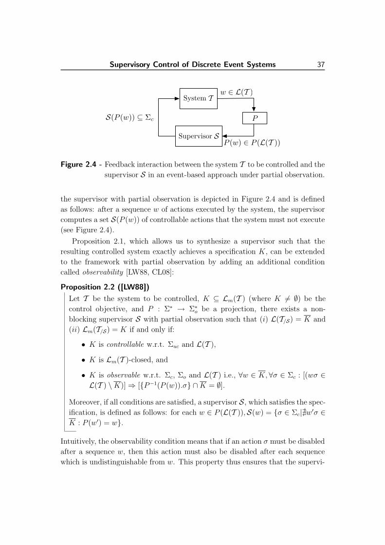
Supervisory Control of Discrete Event Systems 37
S(P (w)) ⊆ Σc
T
S
System
Supervisor
P
P (w) ∈ P (L(T ))
w ∈ L(T )
Figure 2.4 - Feedback interaction between the system T to be controlled and the
supervisor S in an event-based approach under partial observation.
the supervisor with partial observation is depicted in Figure 2.4 and is defined
as follows: after a sequence w of actions executed by the system, the supervisor
computes a set S(P (w)) of controllable actions that the system must not execute
(see Figure 2.4).
Proposition 2.1, which allows us to synthesize a supervisor such that the
resulting controlled system exactly achieves a specification K, can be extended
to the framework with partial observation by adding an additional condition
called observability [LW88, CL08]:
Proposition 2.2 ([LW88])
Let T be the system to be controlled, K ⊆ Lm(T ) (where K 6= ∅) be the
control objective, and P : Σ∗ → Σ∗o be a projection, there exists a non-
blocking supervisor S with partial observation such that (i) L(T/S) = K and
(ii) Lm(T/S) = K if and only if:
• K is controllable w.r.t. Σuc and L(T ),
• K is Lm(T )-closed, and
• K is observable w.r.t. Σc, Σo and L(T ) i.e., ∀w ∈ K,∀σ ∈ Σc : [(wσ ∈L(T ) \K)]⇒ [{P−1(P (w)).σ} ∩K = ∅].
Moreover, if all conditions are satisfied, a supervisor S, which satisfies the spec-
ification, is defined as follows: for each w ∈ P (L(T )),S(w) = {σ ∈ Σc|@w′σ ∈K : P (w′) = w}.
Intuitively, the observability condition means that if an action σ must be disabled
after a sequence w, then this action must also be disabled after each sequence
which is undistinguishable from w. This property thus ensures that the supervi-

38 Chapter 2
x1
x2
x3
x4
x5
x6
a
a
b
b
Figure 2.5 - System without an optimal supervisor.
sor is coherent w.r.t. the actions that it forbids, since it inhibits the same set of
actions after the sequences of actions that it does not distinguish. Therefore, a
correct supervisor must satisfy the observability condition or at least a stronger
property to define a coherent control policy w.r.t. its partial observation. The
time complexity to test the observability property is polynomial [Tsi89].
A similar result also exists for the case where the non-blocking property must
not be ensured [LW88].
When the conditions of Proposition 2.2 do not hold, the computation of an
optimal supervisor S such that Lm(T/S) ⊆ K is not always possible, because
the class of observable sublanguages of K is not closed under union and hence
there does not always exist a supremal observable and controllable sublanguage
of K [LW88]. The following example illustrates this property:
Example 2.3
In the system T depicted in Figure 2.5, (i) the set of states X = {xi | i ∈ [1, 6]},(ii) the set of initial states X0 = {x1, x2}, (iii) the set of final states Xm = X,
and (iv) all transitions are controllable and unobservable. The specification K
is equal to {ε, a, b}. There are three supervisors which satisfy this specification:
• the supervisor S1 which always forbids the actions a and b: L(T/S1) =
{ε}.
• the supervisor S2 which always forbids the action a: L(T/S2) = {ε, b}.
• the supervisor S3 which always forbids the action b: L(T/S3) = {ε, a}.
Therefore, there is no optimal solution, because the supervisors S2 and S3 are
incomparable.
Various approaches have then been developed to overcome this problem and we

Supervisory Control of Discrete Event Systems 39
mention two of them:
• Considering a weaker problem by computing a maximal supervisor. A super-
visor S is maximal if, for each supervisor S ′ such that Lm(T/S′) ⊆ K, we
have that Lm(T/S′) 6⊃ Lm(T/S). In [RP05], Riedweg and Pinchinat work on
this problem. They prove that it is decidable and they propose an algorithm
solving it with a 2EXP-TIME(|ψ| × |P |) complexity (where |ψ| is the size of
the specification and |P | is the size of the system).
• Considering some situations where the supremal observable and controllable
sublanguage of K exists. That is, for example, the case when Σc ⊆ Σo. Indeed,
under this assumption, the controllability and observability properties imply
the normality property [KGM91], which is formally defined as follows:
Definition 2.1 (Normality)
Let L (with L = L) and K (with K ⊆ L) be two languages over Σ and P :
Σ∗ → Σ∗o be a projection, K is normal w.r.t. P and L ifK = P−1(P (K))∩L.
In other words, each behavior of K can be recovered from L and from the
behaviors P−1(P (K)) that are undistinguishable from K. This property is
interesting, because the class of normal sublanguages of a language K is closed
under union and hence there always exists a supremal controllable and normal
sublanguage (denoted by K↑(CN)) of K. Consequently, when Σc ⊆ Σo, an
optimal supervisor S such that Lm(T/S) ⊆ K always exists, since, in this case,
the controllability and observability properties imply the normality property.
It is obtained by computing a supervisor such that the resulting controlled
system achieves exactly K↑(CN) [KGM91].
Decentralized Supervisory Control. In the previous approaches, the sys-
tem is controlled by a single supervisor, but this framework is not suitable for
the control of some systems like the distributed systems. Indeed, these sys-
tems are generally composed of several subsystems acting in parallel and located
in different sites. It is thus more appropriate to have several supervisors that
control the system to ensure the desired properties. The decentralized frame-
work [RW92b, YL02, CL08] follows this approach. It has been widely studied in
the past years and has shown its usefulness in several domains like manufactur-
ing systems, communication network protocols,. . . [RW92a]. In this approach,
the system is controlled by n local supervisors. Each supervisor has its own

40 Chapter 2
PnP1. . .
...
Fusion
P1(w) ∈ P1(L(T ))
Pn(w) ∈ Pn(L(T ))Sn(Pn(w)) ⊆ Σn,c
S1(P1(w)) ⊆ Σ1,c
Sd(w) w ∈ L(T )TSystem
S1Supervisor
Supervisor Sn
Figure 2.6 - Feedback interaction between the system T to be controlled and the
n local supervisors Si (∀i ∈ [1, n]) in a decentralized event-based
approach.
view of the system and its own set of controllable actions. Indeed, due to the
distributed nature of the system to be controlled, the supervisors observe the
system through different sets of sensors (these sets can overlap) and control it
by means of different sets of actuators (these sets can also overlap). Moreover,
there is a coordination mechanism (called fusion rule) defining the global control
to be applied to the system. This global control is computed from the control
decisions of each local supervisor [CL08]. In the decentralized framework, we
have no information regarding the structure of the distributed system to be con-
trolled while the computation of the supervisors. Therefore, the computation
of the local supervisors must be performed on the model of the global system
resulting from the parallel composition of each subsystem.
More precisely, each local supervisor Si (∀i ∈ [1, n]) can control the set of
actions Σi,c and cannot control the set of actions Σi,uc. The subsets Σ1,c, . . . ,Σn,c
are not necessarily disjoint. The set of actions that can be controlled by at
least one controller is denoted by Σc and is defined by Σcdef=⋃n
i=1 Σi,c and the
set of actions that cannot be controlled is denoted by Σuc and is defined by
Σucdef= Σ \ Σc. Moreover, each local supervisor Si can observe the set of actions
Σi,o and cannot observe the set of actions Σi,uo (the subsets Σ1,o, . . . ,Σn,o are not
necessarily disjoint). The partial observation of the supervisor Si (∀i ∈ [1, n])
is modeled by the projection Pi : Σ∗ → Σ∗i,o. The feedback interaction between
the system and the local supervisors is depicted in Figure 2.6 and works as
follows. After a sequence w of actions executed by the system, each supervisor
Si computes its own set Si(Pi(w)) of actions that it proposes to forbid. Next, the

Supervisory Control of Discrete Event Systems 41
global control applied to the system is the fusion, according to some rule to be
defined, of the control decisions of each supervisor. There exist different fusion
rules in the literature and we mention two of them:
• the conjunctive architecture: the fusion rule is defined by the union of forbid-
den actions and is given by the function Rc : L(T ) → 2Σc , which is defined,
for each w ∈ L(T ), by:
Rc(w)def=
n⋃i=1
Si(Pi(w)) (2.1)
This architecture is called conjunctive, because it is defined by the intersection
of enabled actions1.
• the disjunctive architecture: the fusion rule is defined by the intersection of
forbidden actions and is given by the function Rd : L(T ) → 2Σc , which is
defined, for each w ∈ L(T ), by:
Rd(w)def=
n⋂i=1
Si(Pi(w)) (2.2)
This architecture is called disjunctive, because it is defined by the union of
enabled actions.
A decentralized supervisor Sd is then defined by a pair 〈(Si)ni=1,R〉 i.e., by n
local supervisors Si coordinated by a fusion rule R. The controlled system, that
it defines, is denoted by T/Sd.
A fundamental result for the decentralized control (with a conjunctive archi-
tecture) is given by the following proposition:
Proposition 2.3 ([RW92b, RDFV88])
Let T be the system to be controlled, K ⊆ Lm(T ) (where K 6= ∅) be the
control objective, Σi,c and Σi,uc (∀i ∈ [1, n]) be a partition of Σ, Σc =⋃n
i=1 Σi,c,
Σuc = Σ \ Σc, Σi,o and Σi,uo (∀i ∈ [1, n]) be a partition of Σ, Σo =⋃n
i=1 Σi,o,
Σuo = Σ\Σo, and Pi : Σ∗ → Σ∗i,o (∀i ∈ [1, n]) be a projection, there exists a non-
blocking decentralized supervisor Sd = 〈(Si)ni=1,Rc〉 such that (i) L(T/Sd
) = K,
and (ii) Lm(T/Sd) = K if and only if:
• K is controllable w.r.t. Σuc and L(T ),
1In the literature, a supervisor generally gives the actions that are enabled.

42 Chapter 2
• K is Lm(T )-closed, and
• K is CP-coobservable w.r.t. Σi,c, Σi,o (∀i ∈ [1, n]) and L(T ) i.e.,
∀w ∈ K,∀σ ∈ Σc : [wσ ∈ L(T ) \ K] ⇒ [∃i ∈ [1, n] : (σ ∈Σi,c) ∧ ({P−1
i (Pi(w)).σ} ∩K = ∅)].
Thus, a decentralized supervisor such that the resulting controlled system ex-
actly achieves the specification, can be computed if and only if the controllabil-
ity, Lm(T )-closure and CP-coobservability conditions hold. This last condition
means that if an action σ must be disabled after a sequence w, then at least
one of the supervisors, that control σ, proposes to forbid this action after each
sequence that it does not distinguish from w. The time complexity to test the
CP-coobservability property is polynomial [RW95].
A similar result exists for the disjunctive architecture [YL02].
One can note that the centralized control under partial observation is a par-
ticular case of the decentralized control. It corresponds to the case where the
number n of local supervisors is equal to 1.
When a specification K is not CP-coobservable, we would like to compute
a non-blocking and correct supervisor such that the resulting controlled system
achieves a subset of K. But, this is, in general, not possible:
Proposition 2.4 ([Thi05])
Let T be the system to be controlled, K ⊆ Lm(T ) (where K is not CP-
coobservable) be the control objective, Σi,c and Σi,uc (∀i ∈ [1, n]) be a partition
of Σ, Σc =⋃n
i=1 Σi,c, Σuc = Σ \ Σc, Σi,o and Σi,uo (∀i ∈ [1, n]) be a partition
of Σ, Σo =⋃n
i=1 Σi,o, Σuo = Σ \ Σo, and Pi : Σ∗ → Σ∗i,o (∀i ∈ [1, n]) be
a projection, the problem, which consists in deciding if there exists a non-
blocking decentralized supervisor Sd = 〈(Si)ni=1,Rc〉 such that Lm(T/Sd
) ⊆ K
is undecidable.
However, when the non-blocking requirement is relaxed, the problem becomes
decidable [RW95].
Several approaches have been developed to improve the control policy in the
decentralized framework and we mention two of them:
• Adding communication between the supervisors [BL98, BL00, XK09, Tri02].
In [BL00], Barrett and Lafortune formalize a decentralized framework with
Supervisory Control of Discrete Event Systems 43
communication by specifying the communication architecture and the kind of
information exchanged. They assume that there are no communication de-
lays and notably give a necessary and sufficient condition for the existence
of solutions achieving exactly a control specification (defined by a language).
In [XK09], Kumar and Xu propose an algorithm, which computes, for each
local supervisor, an estimate of the current state of the system. To compute
a good state estimate, the local supervisors exchange information: they send,
to the other local supervisors, the actions that they receive from the sys-
tem. In this framework, the communication delays are unbounded. In [Tri02],
Tripakis studies the time complexity of some problems related to the decen-
tralized control with communication. The specification is given by a set φ
of responsiveness properties over an alphabet Σ. A responsiveness property
is a formula of the form a b (where a, b ∈ Σ) and it is satisfied by a (fi-
nite or infinite) string ` over Σ if an action b eventually occurs after every
action a in `. The problem under consideration consists in deciding if there
exists a decentralized supervisor Sd such that the maximal language Lmax of
the controlled system T/Sdsatisfies φ. This language Lmax is defined by all
infinite strings of the controlled system and all finite strings that cannot be
extended by an action of Σ (i.e., the system is in a deadlocking state). The
author proves that the problem is undecidable when there is no communica-
tion or when the communication delays are unbounded. He conjectures that
the problem is decidable when the communication delays are bounded.
• Defining local supervisors with conditional control decision. Usually, in the de-
centralized framework, the local supervisors propose unconditional decisions
i.e., they propose either to forbid or to allow an action. In more elaborate
architectures, they may propose conditional decisions i.e., control decisions
which depend on the decisions of the other supervisors. For example, a su-
pervisor can propose to allow an action if no supervisor proposes to forbid
it. In [YL04], Yoo and Lafortune propose a decentralized framework where
there are four control decisions: enable, disable, disable if nobody enables
and enable if nobody disables. They notably give a necessary and sufficient
condition for the existence of a decentralized supervisor such that the result-
ing controlled system exactly achieves a desired specification (defined by a
language). In [Ric03], Ricker and Rudie propose a decentralized framework
with four possible control decisions: enable, disable, conditional disable, do
not know. A local supervisor makes its control decision based on its own
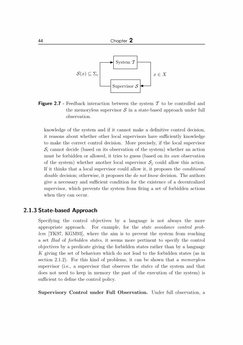
44 Chapter 2
T
S
x ∈ XS(x) ⊆ Σc
System
Supervisor
Figure 2.7 - Feedback interaction between the system T to be controlled and
the memoryless supervisor S in a state-based approach under full
observation.
knowledge of the system and if it cannot make a definitive control decision,
it reasons about whether other local supervisors have sufficiently knowledge
to make the correct control decision. More precisely, if the local supervisor
Si cannot decide (based on its observation of the system) whether an action
must be forbidden or allowed, it tries to guess (based on its own observation
of the system) whether another local supervisor Sj could allow this action.
If it thinks that a local supervisor could allow it, it proposes the conditional
disable decision; otherwise, it proposes the do not know decision. The authors
give a necessary and sufficient condition for the existence of a decentralized
supervisor, which prevents the system from firing a set of forbidden actions
when they can occur.
2.1.3 State-based Approach
Specifying the control objectives by a language is not always the more
appropriate approach. For example, for the state avoidance control prob-
lem [TK97, KGM93], where the aim is to prevent the system from reaching
a set Bad of forbidden states, it seems more pertinent to specify the control
objectives by a predicate giving the forbidden states rather than by a language
K giving the set of behaviors which do not lead to the forbidden states (as in
section 2.1.2). For this kind of problems, it can be shown that a memoryless
supervisor (i.e., a supervisor that observes the states of the system and that
does not need to keep in memory the past of the execution of the system) is
sufficient to define the control policy.
Supervisory Control under Full Observation. Under full observation, a

Supervisory Control of Discrete Event Systems 45
supervisor S is a function X → 2Σc which interacts with the system T in a
feedback manner as illustrated in Figure 2.7: when the system T reaches a state
x, the supervisor observes that T is in x and it computes, from this information,
a set of controllable actions that the system cannot execute. One can note
that the supervisor S is memoryless i.e., its control decisions are only based on
the current information received from the system. The controlled system T/S =
〈X,X0, Xm,Σ,∆/S〉 must satisfy the control objectives and its transition relation
∆/S is defined as follows: ∆/Sdef= {〈x1, σ, x2〉 | (〈x1, σ, x2〉 ∈ ∆) ∧ (σ 6∈ S(x1))}.
Thus, ∆/S corresponds to a restriction of ∆.
A well-known result in this framework is given by the following proposi-
tion [Ush89]:
Proposition 2.5 ([Ush89])
Let T be the system to be controlled, and Bad ⊆ X be the set of forbidden
states, there exists a memoryless supervisor S such that2:
• ReachableT/SΣ (X0) ∩Bad = ∅, and
• S is optimal i.e., for each supervisor S ′ such that ReachableT/S′
Σ (X0) ∩Bad = ∅, we have that Reachable
T/S′
Σ (X0) ⊆ ReachableT/SΣ (X0).
if and only if X0 ∩ CoreachTΣuc(Bad) = ∅.
Moreover, if this condition is satisfied, a supervisor S, which satisfies the
specification, is defined as follows: for each x ∈ X \ CoreachTΣuc(Bad),
S(x)def= {σ ∈ Σc | ∃x′ ∈ CoreachTΣuc
(Bad) : 〈x, σ, x′〉 ∈ ∆}.
This property means that there exists an optimal supervisor which prevents the
system from reaching Bad if and only if a forbidden state cannot be reached
from an initial state of the system T by a sequence of uncontrollable transitions.
The condition in Proposition 2.5 can be tested in polynomial time.
An optimal supervisor can also be computed (when a solution exists) when
the deadlock free or non-blocking property must be ensured. For that, we first
compute the set of states leading uncontrollably to Bad and we add them to
the set of forbidden states. Next, if we make unreachable these states, there
may be blocking (resp. deadlocking) states in the resulting controlled system.
We thus add these blocking (resp. deadlocking) states to the set of forbidden
2The reachability and coreachability operators are respectively defined in Definitions 1.10and 1.9.

46 Chapter 2
states. But, there can then be new states leading uncontrollably to the set of
forbidden states. We thus repeat these two steps until stabilization and we then
obtain a set denoted by Ibl(Bad) (resp. Idf (Bad)). If Ibl(Bad) ∩ X0 = ∅ (resp.
Idf (Bad) ∩X0 = ∅), then there exists an optimal supervisor which prevents the
system from reaching Bad and which ensures the non-blocking (resp. deadlock
free) property. This supervisor is defined as follows: for each x ∈ X \ Ibl(Bad),S(x) = {σ ∈ Σc | ∃x′ ∈ Ibl(Bad) : 〈x, σ, x′〉 ∈ ∆} (resp. for each x ∈ X\Idf (Bad),S(x) = {σ ∈ Σc | ∃x′ ∈ Idf (Bad) : 〈x, σ, x′〉 ∈ ∆}).
Remark 2.1
In [GM05], Gaudin and Marchand consider the problem described in Proposi-
tion 2.5 in a modular framework where the system to be controlled is given by
a collection of n subsystems. They provide an algorithm which computes an
optimal supervisor for this problem by performing the computations locally on
each subsystem. These local computations allow them to avoid the combina-
torial explosion of the number of states resulting from the parallel composition
of the subsystems.
Let us now explain how the event-based approach and the state-based ap-
proach can be linked.
The event-based approach can be used to compute an optimal supervisor
which prevents the system T from reaching a set Bad of forbidden states. For
that, we first define the automaton T ′ = 〈X \ Bad,X0 \ Bad,Xm \ Bad,Σ,∆〉.Next, we compute a supervisor such that the resulting controlled system achieves
the supremal controllable sublanguage of L(T ′) w.r.t. Σuc and L(T ′), and this
supervisor is actually an optimal solution which prevents the system from reach-
ing Bad3.
Inversely, the state-based approach can be used to compute a super-
visor such that the resulting controlled system achieves the supremal
controllable sublanguage of a specification K. For that, we compute
the synchronous product of the automaton T and of the automaton
Tk = 〈Xk, (X0)k, (Xm)k,Σ,∆k〉, which generates the language K. That
gives an automaton T ′ = 〈X × Xk, X0 × (X0)k, Xm × (Xm)k,Σ,∆′〉 such that
L(T ′) = L(T ) ∩ L(Tk). Next, the set Bad of forbidden states is defined by
Bad = {〈x, xk〉 ∈ X × Xk | ∃σ ∈ Σuc,∃x′ ∈ X : [(〈x, σ, x′〉 ∈ ∆) ∧ (@x′k ∈ Xk :
〈〈x, xk〉, σ, 〈x′, x′k〉〉 ∈ ∆′)]}. Thus, 〈x, xk〉 is considered as a forbidden state if
3The time complexity is then in O(X2) instead of O(X).

Supervisory Control of Discrete Event Systems 47
T
S
x ∈ X
S(y) ⊆ Σc
System
Supervisor
M
y ∈M(x)
Figure 2.8 - Feedback interaction between the system T to be controlled and the
supervisor S in a state-based approach under partial observation.
there exists an uncontrollable transition σ that can be fired from x in T and that
cannot be fired from 〈x, xk〉 in T ′ (i.e., that produces a behavior which does not
belong to K). Finally, we use Proposition 2.5 to compute an optimal supervisor,
which prevents the system T ′ from reaching Bad, and the controlled system
defined by this supervisor achieves the supremal controllable sublanguage of K.
Supervisory Control under Partial Observation. In the framework with
partial observation, the supervisor cannot distinguish some states4. This partial
observation is formally defined by a mask M : X → 2Y which corresponds to a
mapping from the state space X to the power set of an observation space Y and
which can also be seen as a covering of the state space [HTL08, DDR06]. When
the system arrives in a state x, the supervisor receives an observation y ∈M(x)
as information and it defines its control decisions from this information (see
Figure 2.8). In the sequel, we say that a state x is compatible with an observation
y if y ∈M(x).
In [TUK95], Takai et al. consider a framework where the system to be
controlled is deterministic and the partial observation is modeled by a mask
M : X → Y corresponding to a partition of the state space i.e., each state is
compatible with exactly one observation (one can note that this definition of
M is a particular case of the definition where it is defined as a covering of the
state space). They provide a necessary and sufficient condition for the existence
of a supervisor that allows the system to exactly reach the set of states Badc
(where Badc = X \Bad and Bad is the set of forbidden states). This necessary
and sufficient condition, given in Proposition 2.6, uses the following memoryless
4This has to be opposed to the event-based approach where the partial observation is dueto some actions that cannot be observed by the supervisor.
48 Chapter 2
supervisor S with partial observation, which prevents the system from reaching
Bad:
∀y ∈ Y, S(y)def= {σ ∈ Σc | ∃x1 6∈ Bad,∃x2 ∈ Bad : (y = M(x1)) ∧
(〈x1, σ, x2〉 ∈ ∆)} (2.3)
Thus, the supervisor S forbids an action σ in the observation state y if there
exists a state x1 6∈ Bad compatible with y, which leads to a forbidden state by
σ.
Proposition 2.6 ([TUK95])
Let T = 〈X, x0, Xm,Σ,∆〉 be the deterministic system to be controlled, Bad ⊆X be the set of forbidden states, and M : X → Y be a mask, there exists a
memoryless supervisor S such that ReachableT/SΣ (x0) = Badc if and only if
Badc is M -controllable5 i.e., the supervisor S, defined in (2.3), satisfies the
property ReachableT
/ eSΣ (x0) = Badc.
Obviously, if the M -controllability condition holds, the supervisor S is a
solution to this problem. This proposition means that if the system resulting from
the supervision of S does not exactly reach Badc, then no supervisor can satisfy
this requirement. The time complexity to test the M -controllability property is
polynomial [TK97, TK98].
When the M -controllability condition does not hold, Takai and Kodama pro-
vide an algorithm computing a memoryless supervisor such that the resulting
controlled system reaches a subset of Badc [TK97, TK98]. This algorithm is
based on a forward approach and is composed of two parts; in this algorithm,
the set Badc of good states is denoted by Q:
• the computation of the set of safe states Q↑ ⊆ Q where Q↑ def=⋂∞
j=0Qj, with
Qj defined recursively as follows:
Qjdef=
{Q if j = 0
g(Qj−1) otherwise
where, for each Q′ ⊆ Q, the function g(Q′)def= Q ∩
(⋂σ∈Σuc
{x1 ∈ X | ∀x2 ∈X : (〈x1, σ, x2〉 ∈ ∆)⇒ (x2 ∈ Q′)}
). Thus, Q↑ gives the set of states that do
not lead to Bad by a sequence of uncontrollable transitions.
5We give a simplified (and equivalent) version of the definition of M -controllability givenin [TUK95].

Supervisory Control of Discrete Event Systems 49
MnM1. . .
...
Fusion
y1 ∈M1(x)
yn ∈Mn(x)Sn(yn) ⊆ Σn,c
S1(y1) ⊆ Σ1,c
Sd(w) x ∈ XTSystem
S1Supervisor
Supervisor Sn
Figure 2.9 - Feedback interaction between the system T to be controlled and
the n local supervisor Si (∀i ∈ [1, n]) in a decentralized state-based
approach.
• the computation of the supervisor S, which gives the actions that are forbidden
by the supervisor. This function is defined, for each y ∈ Y , by S(y)def= {σ ∈
Σc | ∃x1 ∈ Q↑,∃x2 6∈ Q↑ : (y = M(x1)) ∧ (〈x1, σ, x2〉 ∈ ∆)}. This supervisor
forbids an action σ in the observation y if there exists a safe state x1 ∈ Q↑
compatible with y, which leads to a bad state x2 6∈ Q↑ by σ.
Since the system is finite and the function g is monotonic, all computations
terminate; in particular, there exists an integer n such that Q↑ =⋂n
j=0Qj.
However, this method does not always give a maximal supervisor and no
information is given by the authors regarding the computation of such a solu-
tion. To our knowledge, the deadlock free or non-blocking cases have not been
considered.
In [KGM93], Kumar et al. also provide an algorithm which synthesizes a
supervisor (when a solution exists) such that the resulting controlled system
exactly achieves the set Badc of good states. But their supervisor uses the entire
sequence of observations received from the system to define it control policy (this
supervisor has thus a memory).
In [HTL08], Hill et al. extend the results in [TK97, TK98] by considering
non-deterministic systems to be controlled and masks corresponding to coverings
of the state space.
Decentralized Supervisory Control. In the decentralized state-based ap-
proach, the system is controlled by n local supervisors Si (∀i ∈ [1, n]). Each
supervisor Si controls the set of actions Σi,c and cannot control the set of actions

50 Chapter 2
Σi,uc. The subsets Σ1,c, . . . ,Σn,c are not necessarily disjoint. The set of actions
that can be controlled by at least one controller is denoted by Σc and is defined
by Σcdef=⋃n
i=1 Σi,c. The set of actions that cannot be controlled is denoted by
Σuc and is defined by Σucdef= Σ \ Σc. The partial observation of Si is modeled
by the mask Mi : X → 2Yi . The feedback interaction between the system to
be controlled and the n local supervisors is depicted in Figure 2.9 and works as
follows. When the system arrives in a state x ∈ X, each supervisor receives an
observation yi ∈Mi(x). From this information, Si defines a set Si(yi) of actions,
that it proposes to forbid, and the global control applied to the system is the
fusion, according to some rule to be defined, of the control decisions Si(yi) of all
supervisors.
In [TKU94], Takai et al. work on a decentralized framework, where the fusion
ruleRc is given by the intersection of the actions allowed by each supervisor Si. It
is thus a conjunctive architecture and their decentralized supervisor Sd is defined
by the pair 〈(Si)ni=1,Rc〉. In their framework, the system T = 〈X, x0, Xm,Σ,∆〉
to be controlled is deterministic and the partial observation is modeled, for each
supervisor Si, by a mask Mi : X → Yi corresponding to a partition of the state
space. They provide a necessary and sufficient condition for the existence of a
balanced decentralized supervisor Sd that allows the system to exactly reach the
set of states Badc (where Bad is the set of forbidden states). The decentralized
supervisor Sd is balanced if ∀σ ∈ Σ,∀x, x′ ∈ X : [(x, x′ ∈ ReachableT/SdΣ (x0)) ∧
(〈x, σ, x′〉 ∈ ∆)]⇒ [∀i ∈ [1, n] : σ 6∈ Si(Mi(x))], where ReachableT/SdΣ (x0) denotes
the set of states that are reachable in the system T under the control of Sd.
Thus, for each pair of states x, x′ reachable in the controlled system, if there is
an action σ which can be fired from x to x′, then this action must be allowed
by each local supervisor Si in the observation state Mi(x). Their necessary and
sufficient condition, given in Proposition 2.7, uses the following decentralized
supervisor:
Sd = 〈(Si)ni=1,Rc〉 (2.4)
which prevents the system from reaching Bad. For each i ∈ [1, n], the local
supervisor Si with partial observation is defined as follows:
∀y ∈ Yi, Si(y)def= {σ ∈ Σc | ∃x1 6∈ Bad,∃x2 ∈ Bad : (y = Mi(x1)) ∧
(〈x1, σ, x2〉 ∈ ∆)} (2.5)
Thus, the supervisor Si forbids an action σ in the observation y if there exists a
state x1 6∈ Bad compatible with y, which leads to a forbidden state by σ.

Supervisory Control of Discrete Event Systems 51
Proposition 2.7 ([TKU94])
Let T = 〈X, x0, Xm,Σ,∆〉 be the deterministic system to be controlled, Σi,c
and Σi,uc (∀i ∈ [1, n]) be a partition of Σ, Mi : X → Yi (∀i ∈ [1, n]) be a mask,
and Bad ⊆ X be the set of forbidden states, then there exists a decentralized
supervisor Sd = 〈(Si)ni=1,Rc〉 such that Reachable
T/SdΣ (x0) = Badc if and only
if Badc is n-observable6 i.e., the decentralized supervisor Sd, defined in (2.4),
satisfies the property ReachableT
/ eSdΣ (x0) = Badc.
Obviously, if the n-observability condition holds, the decentralized supervisor Sd
is a solution to this problem. This proposition means that if the system resulting
from the supervision of Sd does not exactly reach Badc, then no decentralized
supervisor can satisfy this requirement.
To our knowledge, the problem of computing a solution that allows the system
to reach a subset of Badc when the n-observability property does not hold and
also the problem which consists in ensuring the deadlock free or non-blocking
property have not been studied in the literature. Moreover, we do not know works
where the local supervisors can communicate or provide conditional decisions.
2.2 Control of Infinite State Systems
In the previous section, we have presented control methods for systems mod-
eled by regular languages or equivalently by finite automata. However, in many
industrial applications, the state space of the model of the system can be in-
finite. For example, the state space is infinite, when the model of the system
uses variables that take their value in an infinite domain. Unfortunately, the
control theory presented in section 2.1 cannot trivially be extended to infinite
state systems, because most of the control problems become undecidable. In the
literature, there are mainly two approaches to overcome this undecidability: ei-
ther we consider subcases, in which the problem we want to solve is decidable,
or we use approximation techniques to compute a correct approximation of the
solution in a finite number of steps.
The formalism of automata is not suitable for the representation of infinite
state systems. Indeed, they cannot always represent these systems with a finite
structure. In the literature, there exist several formalisms to efficiently han-
6We give a simplified (and equivalent) version of the definition of n-observability givenin [TKU94].

52 Chapter 2
p1
p2
t1
(a) p1 contains one to-ken.
p1
p2
t1
(b) t1 has been fired andthe token moves from p1
to p2
Figure 2.10 - A Petri net with two places and one transition.
dle infinite state systems. We can, for example, mention Petri nets [Pet62],
timed automata [AD90], extended automata [SAF09], symbolic transitions sys-
tems [HMR05],. . . In the remainder of this section, we present works related to
the control of infinite state systems modeled by these formalisms.
2.2.1 Controller Synthesis with Petri Nets
An alternative formalism for discrete event systems is provided by Petri
nets [Pet62]. Petri nets are well suitable for the modeling of the concurrent
behavior of distributed systems. They allow us to represent more easily com-
plex systems that cannot compactly be represented by automata, because of the
combinatorial explosion of the number of states. Petri nets are more expressive
than finite automata and they can also represent some infinite state systems.
A Petri net has a finite set of places, a finite set of transitions, and an incidence
relation which indicates the evolution of the system w.r.t. the places and the
transitions. The places and the transitions are connected by directed arcs. An arc
can be directed from a place to a transition or from a transition to a place. For
a given transition t, the input (resp. output) places of t are the places that lead
to (resp. are reachable from) t by a directed arc. In Petri nets, the mechanism,
that indicates whether a transition can be fired, is provided by tokens, which are
assigned to places. A transition t may be fired whenever there is a token in all
input places of t. When it is fired, it consumes these tokens and places tokens
in all output places. Figure 2.10(a) illustrates a Petri net with two places p1

Supervisory Control of Discrete Event Systems 53
p1
p2
cp1
t1
Figure 2.11 - A controlled Petri net with a control place cp1 which controls the
transition t1.
and p2 (p1 contains one token) and with one transition t1; when t1 is fired (see
Figure 2.10(b)) the token moves from p1 to p2. At each step of the execution,
the places have a certain number of tokens and the marking, which indicates the
number of tokens in each place, defines the state of the system at this step. One
can note that a Petri net has an initial marking and can have an infinite number
of markings. A marking m1 covers a marking m2 if, for each place p of the Petri
net, the number of tokens in p for m1 is greater than or equal to the number
of tokens in p for m2. A set M of markings is right-closed if, for each marking
m ∈M , all states, that cover m, are in M .
The control of Petri nets has been developed by Holloway and Krogh [Kro87,
HKG97, KH91]. To control the behavior of Petri nets, they add control places
to the system; this extended model is called controlled Petri net. A control place
is connected to one or several transitions and it inhibits them, when it contains
no token. Figure 2.11 illustrates this control mechanism: the control place cp1
controls the transition t1 and this transition cannot be fired, because cp1 contains
no token.
In [KG05], Garg and Kumar prove that the state avoidance control problem
for Petri nets, which consists in preventing the system from reaching a set of
forbidden states (markings), is undecidable. They also prove that this problem is
decidable when the set of forbidden markings is right-closed and they provide an
algorithm which computes the optimal control policy. In [Kro87, KH91, KH90],
Holloway and Krogh define several assumptions which imply that the Petri nets
they consider have a finite number of different markings and are equivalent to
automata. They give a necessary and sufficient condition for the existence of an

54 Chapter 2
optimal control policy which satisfies the control objective. They also provide
this control policy, when this condition is satisfied. In [HB91], Baosheng and
Hoaxun introduce the concept of partial observation and define a distributed
control for controlled Petri nets where the aim is to prevent the system from
reaching a set of forbidden markings. Each local controller has only a partial
observation of the system, which is modeled by a function mapping a marking
onto an observation class. A controller is unable to distinguish between the
markings of a same observation class and it must then produce the same control
for these markings. They solve the problem by adding coordination places to
the system in order to synchronize the controllers and by using the approach of
Holloway and Krogh [KH90] to prevent the system from reaching the forbidden
states.
When the specification is given by a language generated by a Petri net (note
that this language is not necessarily regular), it has been shown in [Sre93] that
deciding if this language is controllable is undecidable. However, the problem is
decidable when the specification language is generated by a deterministic Petri
net [Sre93]. In [KH96], Holloway and Kumar present an algorithm computing the
optimal control policy when the system to be controlled is a deterministic Petri
net and the specification is a regular language. The main idea of their algorithm
consists in restricting this problem into a state avoidance control problem, which
is obtained by computing the synchronous product of the system to be controlled
and of the specification.
Works ensuring the deadlock free property and the non-blocking property
have also been developed (e.g., [VNJ90, KH92]).
2.2.2 Control of Timed Automata
The formalism of timed automata is a widely used model for representing real-
time systems. A timed automaton [AD90] has a finite set of locations, a finite set
of actions, a finite set of real-valued clocks and a finite set of transitions. Each
transition is labeled by an action, has a guard which depends on the clocks, and
can reset clocks.
Figure 2.12 illustrates a timed automaton which has two locations `1 and `2,
one clock x and two actions a and b. The transitions δ1 can be fired when the
value of the clock x is less than or equal to 4. When it is fired, this clock is reset.
A state of the underlying labeled transition system of a timed automaton Tis given by a pair 〈x, t〉 where x is a location of T and t is the instant in which the

Supervisory Control of Discrete Event Systems 55
δ2 = 〈b;x ≤ 10;−〉δ1 = 〈a;x ≤ 4;x := 0〉
!2!1
Figure 2.12 - An example of timed automata.
system is in x (more precisely, t gives the value of the clocks). Since the clocks
have real values, the number of states of this labeled transition system can be
infinite. However, a timed automaton can be translated into a finite automaton,
called region automaton, which abstracts timed behaviors of the timed automaton
into untimed behaviors and which preserves the semantics of the system. This
abstraction has been proposed by Alur and Dill [AD90, AD94] and is the core of
several decidability results (e.g. reachability, coreachability, emptiness, . . . ) for
the model of timed automata.
The control mechanism for timed automata consists in partitioning the set
of actions into the subset of controllable actions and the subset of uncontrollable
actions. Most of the works on the control of timed automata are based on game
theory where the aim is to compute a winning strategy. A winning strategy is a
function that tells precisely what the controller has to do in order to satisfy the
requirements [MPS95].
In [AMPS98], Asarin et al. consider a specification defined by a set of for-
bidden states and they provide an algorithm which computes the set of winning
strategies for this specification. These strategies can be computed thanks to the
concept of region automaton. In [HK99], Henzinger and Kopke prove that the
safety control problem, which consists in deciding if there is a winning strategy
for a specification given by a set of forbidden states, is EXPTIME-complete.
In [CDF+05], an efficient approach computing a solution for this problem is
defined and implemented in the tool Uppaal TiGA.
If the specification is defined by a timed automaton over infinite words, the
control problem, which consists in deciding if there is a winning strategy for this
specification, is undecidable [DM02]. However, the problem is decidable when
the specification is given by a deterministic finite automaton; the problem is
actually 2EXPTIME-complete.
The concept of partial observation has also been developed for the control
of timed automata. This partial observation means that the controller does not
observe certain actions and it is modeled by a partition of the set of actions
56 Chapter 2
into the subset of observable actions and the subset of unobservable actions.
In [BDMP03], Bouyer et al. suppose that only uncontrollable actions can be un-
observable. They prove that the safety control problem under partial observation
is undecidable. They also prove that the control problem under partial obser-
vation for specifications defined by deterministic timed automata over infinite
words is undecidable.
2.2.3 Control of Systems using Variables
For practical reasons, complex systems are generally modeled by using variables.
Finite automata are not suitable enough to represent these systems, specially
when the domain of the variables is infinite. There exist several formalisms
using variables and we mention some of them below.
In [KG05], Garg and Kumar use the assignment program framework to model
infinite state systems [KGM93]. This formalism is composed of variables and of
a finite sequence of instructions. Each instruction is labeled by an action (the
set of actions is finite), and has a guard (which depends on the variables) and
an assignment statement (which assigns new values to the variables). They
prove that the problem (called state avoidance control problem) that consists in
deciding if there is a controller with full observation, which prevents the system
from reaching a set of forbidden states, is undecidable.
In [SAF09], Skoldstam et al. use the model of Extended Automata. This
model is similar to the formalism of automata except that it has variables and
each transition is composed of an action (the set of actions is finite), a guard
(which depends on the variables), and an assignment (which assigns new values
to the variables). They provide a method which takes a collection of extended
automata as input and which efficiently translates them into an automaton to use
the classical supervisory control theory on this system. To ensure the termination
of the computations, they suppose that the domain of the variables is finite.
In [LJM05], Le Gall et al. use the model of symbolic transition sys-
tems [HMR05]. This model is defined by a finite set of variables, an infinite
set of actions, and a finite set of symbolic transitions. Each transition is labeled
by an action, and has a guard and an update function (a detailed description of
this model is given in chapter 3). They use symbolic techniques to tackle the state
avoidance control problem and use abstract interpretation techniques [CC77] to
overcome the undecidability of this problem. These techniques ensure that their
algorithm, which synthesizes controllers for the state avoidance control prob-

Supervisory Control of Discrete Event Systems 57
lem, always terminates, but they may overapproximate some computations. The
computed controllers are memoryless and have a full observation of the system.
This work has been extended in [GD07] to tackle the control of concurrent
systems modeled by extended automata (the specification is defined by a lan-
guage). The domain of the variables can be infinite, which explains the use of
abstract interpretation to ensure the termination of the computations.
2.3 Conclusion
In this chapter, we have outlined the basic concepts of supervisory control the-
ory for finite discrete event systems by presenting some important results. The
control of infinite state systems also received attention in the literature and we
have presented interesting results in this domain. This topic is harder, because
most of the control problems are undecidable. To define effective algorithms
(i.e., which always terminate), the authors generally restrict their attention to
particular cases in which the problems are decidable. Few works use abstract
interpretation techniques to ensure the termination of the algorithms. We can,
nevertheless, mention [LJM05], where this approach is used to compute memo-
ryless controllers with full observation for the state avoidance control problem.
As explained in the introduction of this thesis, we are interested in the con-
trol of infinite state systems with partial observation. Our aim is to define
effective algorithms, which synthesize controllers for these systems. To ensure
the termination of our algorithms, we use, as in [LJM05], abstract interpretation
techniques.

58 Chapter 2
Part II
Control of Infinite State Systems
59

Chapter
3Synthesis of Centralized Memoryless
Controllers with Partial Observation
for Infinite State Systems
In this chapter, we address the state avoidance control problem where the
aim is to synthesize controllers which prevent the system from reaching
a set of forbidden states. We place ourself in the context of infinite state
systems to be controlled that are partially observed by the controller. Indeed,
to model realistic systems, it is often convenient to manipulate state variables
instead of simply atomic states, allowing a compact way to specify systems han-
dling data. In that case, to provide a homogeneous treatment of these models,
it is convenient to consider variables, whose domain is infinite, and thus systems
with an infinite state space. Moreover, from a control point of view, the con-
troller interacts with the plant through sensors and actuators and, in general,
it has only a partial observation of the system, because these materials have not
an absolute precision or some parts of the plant might not be observed by the
controller.
Our aim is to propose effective algorithms (i.e., which always terminate)
for the control of infinite state systems with partial observation; one can note
that this problem is generally undecidable. We use the notion of mask defined
in [DDR06, HTL08] to model partial observation. In these works, a mask is de-

62 Chapter 3
fined as a covering of the state space and this definition thus generalizes the one
given in [KGM93], where a mask corresponds to a partition of the state space.
The state avoidance control problem that we want to solve in undecidable. To
overcome this negative result, we follow the approach defined in [LJM05] where
an effective algorithm synthesizing memoryless controllers with full observation
is obtained by using abstract interpretation techniques. These techniques over-
approximate some computations to ensure their termination. In this chapter,
we provide effective algorithms computing memoryless controllers with partial
observation. In the next chapter, we extend our method to synthesize controllers
with memory and online controllers. Our algorithms have been implemented to
be evaluated experimentally.
An infinite state system can obviously be modeled by an automaton, but the
lack of structure of this formalism makes very hard the manipulation of such
systems. To work with these systems, it is more convenient to use the formalism
of symbolic transition systems (or STS for short), which allow us to represent
infinite state systems with a finite syntax; we define this model in section 3.1. In
section 3.2, we explain how the state avoidance control problem can be used to
solve safety properties. Next, in section 3.3, we formally define the control mech-
anisms, that we use, and the state avoidance control problem. In section 3.4,
we define a semi-algorithm (i.e., which does not always terminate) which syn-
thesizes controllers for the state avoidance control problem and then we explain
how to use abstract interpretation to obtain an effective algorithm (i.e., which al-
ways terminates). In section 3.5, we extend our method to synthesize controllers
which ensure that the controlled system is deadlock free and, in section 3.6, we
explain why our approach cannot be used for the non-blocking case. Finally, in
section 3.7, we describe the experimental results obtained with our method.
3.1 Symbolic Transition Systems
To model realistic systems, it is often convenient to manipulate state variables
instead of simply atomic states. The techniques and associated tools derived from
the labeled transition systems do not explicitly take into account the data as the
underlying model of transition systems which implies that the variables must be
instantiated during the state space exploration and analysis. This enumeration
of the possible values of the variables leads to the classical state space explosion
when these variables take their values in a finite set, but may also render the
computations infeasible whenever the domain of the variables is infinite. In this
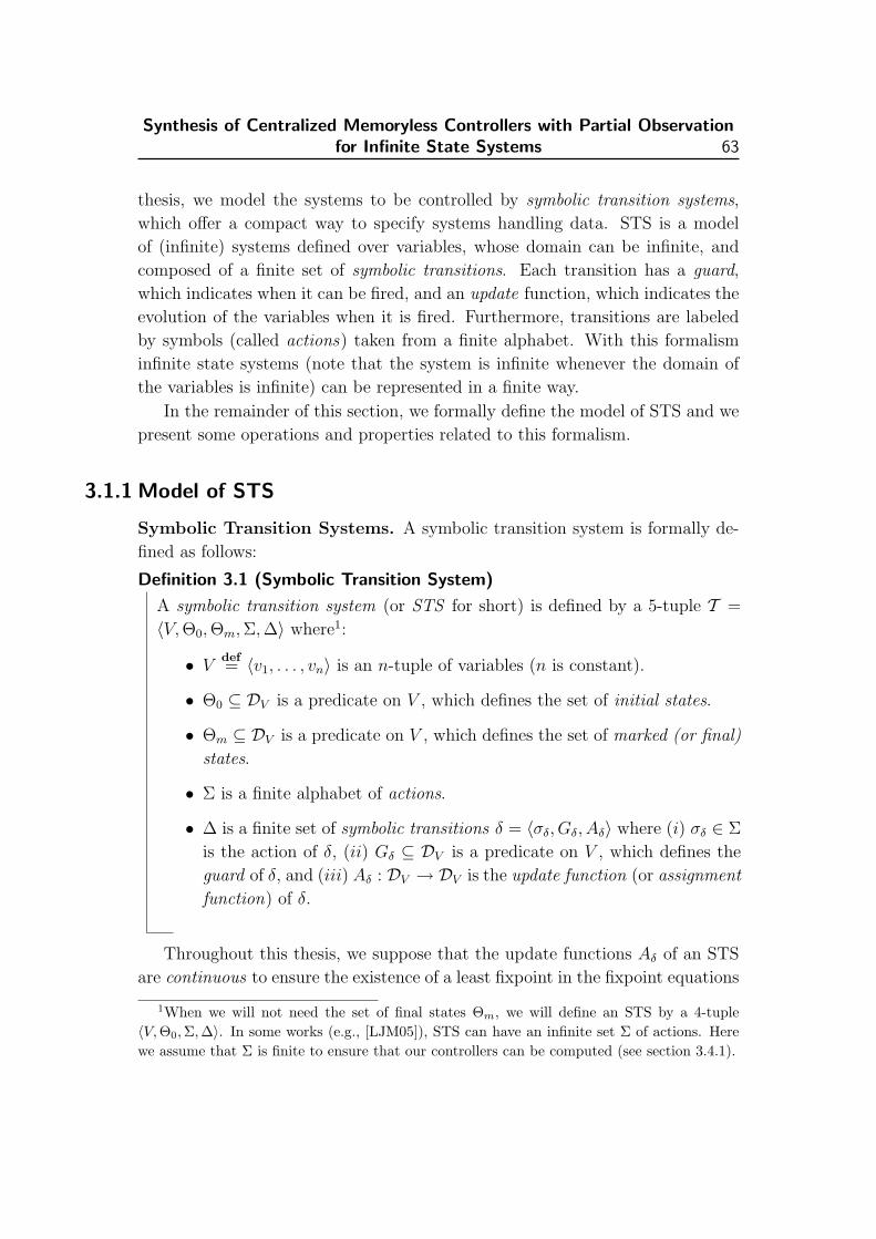
Synthesis of Centralized Memoryless Controllers with Partial Observationfor Infinite State Systems 63
thesis, we model the systems to be controlled by symbolic transition systems,
which offer a compact way to specify systems handling data. STS is a model
of (infinite) systems defined over variables, whose domain can be infinite, and
composed of a finite set of symbolic transitions. Each transition has a guard,
which indicates when it can be fired, and an update function, which indicates the
evolution of the variables when it is fired. Furthermore, transitions are labeled
by symbols (called actions) taken from a finite alphabet. With this formalism
infinite state systems (note that the system is infinite whenever the domain of
the variables is infinite) can be represented in a finite way.
In the remainder of this section, we formally define the model of STS and we
present some operations and properties related to this formalism.
3.1.1 Model of STS
Symbolic Transition Systems. A symbolic transition system is formally de-
fined as follows:
Definition 3.1 (Symbolic Transition System)
A symbolic transition system (or STS for short) is defined by a 5-tuple T =
〈V,Θ0,Θm,Σ,∆〉 where1:
• V def= 〈v1, . . . , vn〉 is an n-tuple of variables (n is constant).
• Θ0 ⊆ DV is a predicate on V , which defines the set of initial states.
• Θm ⊆ DV is a predicate on V , which defines the set of marked (or final)
states.
• Σ is a finite alphabet of actions.
• ∆ is a finite set of symbolic transitions δ = 〈σδ, Gδ, Aδ〉 where (i) σδ ∈ Σ
is the action of δ, (ii) Gδ ⊆ DV is a predicate on V , which defines the
guard of δ, and (iii) Aδ : DV → DV is the update function (or assignment
function) of δ.
Throughout this thesis, we suppose that the update functions Aδ of an STS
are continuous to ensure the existence of a least fixpoint in the fixpoint equations
1When we will not need the set of final states Θm, we will define an STS by a 4-tuple〈V,Θ0,Σ,∆〉. In some works (e.g., [LJM05]), STS can have an infinite set Σ of actions. Herewe assume that Σ is finite to ensure that our controllers can be computed (see section 3.4.1).

64 Chapter 3
δ4 = 〈Stop prod;TTDV ; y := 2〉
δ2 = 〈Stop cons;TTDV ; IdDV 〉δ6 = 〈Stop cons′;TTDV ; IdDV 〉
δ5 = 〈Cons′; 0 ≤ y′ ≤ 2, x′ := x′ − 1; y′ := y′ − 1〉
δ3 = 〈Prod;TTDV ;x := x + 1〉 δ7 = 〈Prod′;TTDV ;x′ := x′ + 1〉
δ1 = 〈Cons; 0 ≤ y ≤ 2;x := x− 1, y := y − 1〉
δ9 = 〈Choice X;TTDV ; IdDV 〉δ10 = 〈Choice X ′;TTDV ; IdDV 〉
δ8 = 〈Stop prod′;TTDV ; y′ := 2〉
CX CX′
PX PX′
Choice
Figure 3.1 - Producer and consumer example.
that we will define.
The semantics of an STS is defined by a possibly infinite labeled transition
system (or LTS for short) whose states are valuations of the variables:
Definition 3.2 (Semantics of an STS)
The semantics of an STS T = 〈V,Θ0,Θm,Σ,∆〉 is defined by an LTS [[T ]]def=
〈X,X0, Xm,Σ,∆[[T ]]〉 where:
• X def= DV is the set of states
• X0def= Θ0 is the set of initial states
• Xmdef= Θm is the set of final states
• Σ is the set of labels
• ∆[[T ]] ⊆ X × Σ × X is the transition relation defined by ∆[[T ]]def=
{〈~ν1, σ, ~ν2〉 | ∃ 〈σδ, Gδ, Aδ〉 ∈ ∆ : (σδ = σ) ∧ (~ν1 ∈ Gδ) ∧ (~ν2 = Aδ(~ν1))}.
An STS thus begins its execution in an initial state. Then, in any state, a
transition can be fired only if its guard is satisfied and, in this case, the variables
are updated according to the update function.

Synthesis of Centralized Memoryless Controllers with Partial Observationfor Infinite State Systems 65
Remark 3.1
The formalism presented in Definition 3.1 does not allow us to explicitly define
locations. But, this model is actually equivalent to a model with explicit
locations [JMR06], because a variable of enumerated type can always be added
to encode the locations. To have clearer illustrations in our examples, the
figures, that depict STS, will have explicit locations that will be encoded by
this mechanism.
Example 3.1
The STS2 of Figure 3.1 is a system of stock management. Two units produce
and send (consume) two kinds of parts X and X ′. The STS has a tuple
V = 〈`, x, x′, y, y′〉 of five variables, where (i) ` ∈ {CX,PX,Choice,CX′,PX′}gives the current location of the system, (ii) x (resp. x′) gives the number
of parts X (resp. X ′) and (iii) y (resp. y′) gives the number of parts X
(resp. X ′) that can be produced. The initial state is 〈Choice, 0, 0, 0, 0〉. The
choice of the kind of parts to produce is performed in the location Choice:
the action Choice X (resp. Choice X ′) allows the system to produce parts
X (resp. X ′). In the location PX (resp. PX′), the action Prod (resp. Prod′)
produces a part X (resp. X ′) whereas the action Stop prod (resp. Stop prod′)
stops the production process. In the location CX (resp. CX′), the action Cons
(resp. Cons′) consumes a part X (resp. X ′) and the action Stop cons (resp.
Stop cons′) stops the consumption process. The variables y and y′ ensure that
at most three parts can be consumed in each consumption cycle.
Generated and Marked Languages. The language L(T ), which represents
the set of finite words w generated by T , is defined by L(T )def= L([[T ]]) and the
language Lm(T ), which represents the set of finite words w marked by T , is
defined by Lm(T )def= Lm([[T ]]).
Reachability and Coreachability. A state ~ν1 is reachable (resp. coreachable)
from a state ~ν2 in an STS T = 〈V,Θ0,Θm,Σ,∆〉 if and only if it is reachable
(resp. coreachable) from ~ν2 in the LTS [[T ]] i.e., it is reachable (resp. coreach-
2For convenience, in the guards and the update functions of the transitions of the system, weomit the conditions and assignments related to the locations. For example, the transition δ2 isdefined by 〈Stop cons;TTDV
; IdDV〉, whereas it should be defined by 〈Stop cons; ` = CX; ` :=
Choice〉.

66 Chapter 3
able) from ~ν2 by a finite sequence of transitions3.
Deterministic Symbolic Transition System. An STS T is deterministic if
and only if the LTS [[T ]] is deterministic4. But deciding if T is deterministic
is generally undecidable [Dub06]. Since it is not always possible to check the
determinism of an STS, we consider a stronger notion of determinism called
structural determinism and defined as follows:
Definition 3.3 (Structural Determinism)
An STS T = 〈V,Θ0,Θm,Σ,∆〉 is structurally deterministic if and only if
∀〈σ1, G1, A1〉 6= 〈σ2, G2, A2〉 ∈ ∆ : (σ1 = σ2)⇒ (G1 ∩G2 = ∅).
The following property shows that the structural determinism implies the deter-
minism:
Proposition 3.1
If an STS T = 〈V,Θ0,Θm,Σ,∆〉 is structurally deterministic, then it is deter-
ministic.
Proof
Let us suppose that T is structurally deterministic and non-deterministic.
The non-determinism of T implies that there exist transitions
〈σ1, G1, A1〉, 〈σ2, G2, A2〉 ∈ ∆ and states ~ν1, ~ν2, ~ν3 ∈ DV such that (i)
σ1 = σ2, (ii) ~ν1 ∈ G1, (iii) ~ν2 = A1(~ν1), (iv) ~ν1 ∈ G2, (v) ~ν3 = A2(~ν1), and
(vi) ~ν2 6= ~ν3. Therefore, T is not structurally deterministic, because the
transitions 〈σ1, G1, A1〉 and 〈σ2, G2, A2〉 are such that (i) σ1 = σ2 and (ii)
G1 ∩G2 6= ∅, which gives a contradiction.
The structural determinism can be checked on an STS if the class of formulae
used to define the predicates allows us to check the satisfiability of the formulae.
3.1.2 Properties and Operations on STS
In this subsection, we recall some properties and operations on STS. This recall
is not exhaustive; we only present the notions that we use in this thesis.
3The formal definition of a reachable (resp. coreachable) state in an LTS is given in Defi-nition 1.5 (resp. Definition 1.6)).
4The formal definition of a deterministic LTS is given in section 1.2.

Synthesis of Centralized Memoryless Controllers with Partial Observationfor Infinite State Systems 67
Notations. Given an STS T = 〈V,Θ0,Θm,Σ,∆〉 and an action σ ∈ Σ, the
notation Trans(σ)def= {〈σδ, Gδ, Aδ〉 ∈ ∆ |σδ = σ} gives the set of transitions
labeled by σ. Given a transition δ ∈ ∆ and two states ~ν1, ~ν2 ∈ DV , ~ν1δ−→ ~ν2
denotes the fact that ~ν2 is reachable from ~ν1 by the transition δ.
Backward and Forward Operators. Given an STS T = 〈V,Θ0,Θm,Σ,∆〉,a subset of transitions D ⊆ ∆, and a subset of actions A ⊆ Σ, we define the
following backward and forward operators:
• the function PreTD : 2DV → 2DV is defined, for each B ⊆ DV , by PreTD(B)def=⋃
〈σ,G,A〉∈D(G ∩ A−1(B))def=⋃〈σ,G,A〉∈D{~ν1 ∈ DV | ∃~ν2 ∈ B : (~ν1 ∈ G) ∧ (~ν2 =
A(~ν1))}. Thus, PreTD(B) gives the set of states that lead to B by a transition
of D.
• the function PostTD : 2DV → 2DV is defined, for each B ⊆ DV , by PostTD(B)def=⋃
〈σ,G,A〉∈D(A(G ∩ B))def=⋃〈σ,G,A〉∈D{~ν1 ∈ DV | ∃~ν2 ∈ B : (~ν2 ∈ G) ∧ (~ν1 =
A(~ν2))}. Thus, PostTD(B) gives the set of states that are reachable from B by
a transition of D
• the function PreTA : 2DV → 2DV is defined, for each B ⊆ DV , by PreTA(B)def=⋃
σ∈A PreTTrans(σ)(B). Thus, PreTA(B) gives the set of states that lead to B by
a transition labeled by an action of A.
• the function PostTA : 2DV → 2DV is defined, for each B ⊆ DV , by PostTA(B)def=⋃
σ∈A PostTTrans(σ)(B). Thus, PostTA(B) gives the set of states that are reachable
from B by a transition labeled by an action of A.
Coreachability and Reachability Operators. Given an STS T =
〈V,Θ0,Θm,Σ,∆〉, a subset of transitions D ⊆ ∆, and a subset of actions A ⊆ Σ,
we define the following functions:
• the function CoreachTD : 2DV → 2DV is defined, for each B ⊆ DV , by
CoreachTD(B)def=⋃
n≥0(PreTD)n(B). Thus, CoreachTD(B) gives the set of states
that lead to B by a sequence of transitions of D.
• the function ReachableTD : 2DV → 2DV is defined, for each B ⊆ DV , by
ReachableTD(B)def=⋃
n≥0(PostTD)n(B). Thus, ReachableTD(B) gives the set of
states that are reachable from B by a sequence of transitions of D.

68 Chapter 3
• the function CoreachTA : 2DV → 2DV is defined, for each B ⊆ DV , by
CoreachTA(B)def= CoreachTTrans(A)(B). Thus, CoreachTA(B) gives the set of states
that lead to B by a sequence of transitions labeled by actions of A.
• the function ReachableTA : 2DV → 2DV is defined, for each B ⊆ DV , by
ReachableTA(B)def= ReachableTTrans(A)(B). Thus, ReachableTA(B) gives the set
of states that are reachable from B by a sequence of transitions labeled by
actions of A.
In this thesis, our algorithms, which synthesize controllers for STS, are based
on reachability and coreachability operations i.e., the main operations consist in
computing the set of states that are reachable or coreachable from a given set
of states. Therefore, our main operations on STS work on sets of states. In our
tool SMACS (see appendix A), the sets of states are symbolically represented
by predicates and the operations on these sets are performed by predicate
transformers, which are functions mapping a predicate to another predicate.
For example, in our tool we compute PreTδ (B) by mapping the predicate
B : DV → {tt, ff} (which is defined, for each ~ν ∈ DV , by B(~ν)def= tt if and only
if ~ν ∈ B) into the predicate PreTδ (B) : DV → {tt, ff} which is defined, for each
~ν1 ∈ DV , by PreTδ (B)(~ν1)def= ∃~ν2 ∈ B : (~ν1 ∈ G) ∧ (~ν2 = A(~ν1)) (where G and A
are respectively the guard and the update function of δ).
Synchronous Product Operator. The synchronous product consists in com-
puting, from two STS T1 and T2, a new STS whose behavior corresponds to the
intersection of the behaviors of T1 and T2. This operation is formally defined as
follows:
Definition 3.4 (Synchronous Product)
Given two STS T1 = 〈V1,Θ0,1,Θm,1,Σ,∆1〉 and T2 = 〈V2,Θ0,2,Θm,2,Σ,∆2〉such that V1 ∩ V2 = ∅, the synchronous product of T1 and T2, denoted by
T1 × T2, is defined by an STS T = 〈V,Θ0,Θm,Σ,∆〉 where:
• V def= V1 ·∪V2
• Θ0def= Θ0,1 ×Θ0,2
• Θmdef= Θm,1 ×Θm,2

Synthesis of Centralized Memoryless Controllers with Partial Observationfor Infinite State Systems 69
• the transition relation ∆ is defined as follows: for each pair of transi-
tions 〈σ,G1, A1〉 ∈ ∆1 and 〈σ,G2, A2〉 ∈ ∆2, we define a new transition
〈σ,G1 ∩ G2, A〉def∈ ∆ where the update function A : DV1 × DV2 →
DV1 ×DV2 is defined, for each ~ν1 ∈ DV1 and ~ν2 ∈ DV2 , by A(〈~ν1, ~ν2〉)def=
〈A1(~ν1), A2(~ν2)〉.
The synchronous product satisfies the two following properties: (i)
L(T ) = L(T1) ∩ L(T2) and (ii) Lm(T ) = Lm(T1) ∩ Lm(T2). Moreover,
the synchronous product of two deterministic (resp. structurally deterministic)
STS is a deterministic (resp. structurally deterministic) STS.
Properties. The deadlock free and non-blocking properties are defined as follows
on STS:
Definition 3.5 (Deadlock Free Property)
An STS T = 〈V,Θ0,Θm,Σ,∆〉 is deadlock free if and only if the LTS [[T ]] is
deadlock free. In other words, T is deadlock free if and only if, for each state
~ν reachable in this system, there exists at least one transition that can be fired
from this state (i.e., ∃〈σ,G,A〉 ∈ ∆ : ~ν ∈ G).
Definition 3.6 (Non-blocking Property)
An STS T = 〈V,Θ0,Θm,Σ,∆〉 is non-blocking if and only if the LTS [[T ]] is
non-blocking.
3.2 State Invariance Properties
As mentioned above, we are interested in the state avoidance control problem,
where the aim is to control the system to satisfy a state invariance property,
which is defined by a set Bad of states that the system must avoid. In this
section, we explain how a safety property can be reduced to a state invariance
property by means of an STS-observer.
State Invariance Property and Safety Property. We first define the con-
cept of state invariance property:

70 Chapter 3
〈Inc;TTDV ;x := x + 1〉
!T1
(a) The system T .
〈Inc;x ≥ 10;V iolate := tt〉!O1 !OVi
〈Inc;TTDV ; IdDV〉〈Inc;x ≤ 9; IdDV〉
(b) The STS-observer O.
Figure 3.2 - An STS T and an STS-observer O for T .
Definition 3.7 (State Invariance Property)
Given an STS T = 〈V,Θ0,Θm,Σ,∆〉, a state invariance property is defined by
a set of states Bad ⊆ DV and the STS T satisfies this state invariance property
if Bad cannot be reached along the execution of T i.e., ReachableT∆(Θ0)∩Bad =
∅.
Now, one can also want to specify more general properties like safety properties.
In this setting a safety property ψ over an alphabet Σ is defined by a set of finite
sequences of actions such that ∀w1 ∈ Σ∗ : (w1 6∈ ψ) ⇒ (∀w2 ∈ Σ∗ : w1.w2 6∈ ψ).
In other words, if a finite sequence violates the property ψ, no extension of this
sequence will satisfy it. The absence of failure is a classical example of safety
properties.
STS-observer. The concept of STS-observer is used to reduce a safety property
to a state invariance property. Given an STS T , an STS-observer of T is an STS
O which is non-intrusive i.e., O satisfies the following property: L(T × O) =
L(T ). The STS O can share some variables with the STS T to observe this
system, but it cannot modify them5. Moreover, this STS has a particular boolean
variable Violate and its set of marking states is given by the set ViolateO which
denotes the set of states in which the variable Violate is equal to tt; one can
note that once Violate becomes true, then so is forever. The language Lm(O)
marked by O corresponds to the set of sequences of actions which lead to a state
where the variable Violate is equal to tt. In fact, an STS-observer encodes the
negation of a safety property ψ and Lm(O) then represents the set of sequences
that violate ψ.
5The synchronous product used to compute T × O is slightly different from the one givenin Definition 3.4, because T and O can share variables.

Synthesis of Centralized Memoryless Controllers with Partial Observationfor Infinite State Systems 71
〈Inc;x ≥ 10;x := x + 1, V iolate := tt〉〈!T1 , !O1 〉 〈!T1 , !OVi〉
〈Inc;TTDV ;x := x + 1〉〈Inc;x ≤ 9;x := x + 1〉
Figure 3.3 - Synchronous product T × O.
Example 3.2
Let us consider the system T = 〈VT , (Θ0)T , (Θm)T ,Σ,∆T 〉 depicted in Fig-
ure 3.2(a) which increments a variable x. This STS has a tuple VT = 〈`T , x〉of two variables where (i) `T ∈ {`T1 } gives the location of the system, and (ii)
x ∈ N0. The set of initial states (Θ0)T = {〈`T1 , 0〉} and the set of marked states
Θm = DVT . An STS-observer, which encodes the negation of the safety prop-
erty ψ = �(x ≤ 10) (i.e., x must always be less than 10), can be defined by the
STS O = 〈VO, (Θ0)O, (Θm)O,Σ,∆O〉 depicted in Figure 3.2(b). This STS has
a tuple VO = 〈`O, x, V iolate〉 of three variables where (i) `O ∈ {`O1 , `OVi} gives
the current location of the system, (ii) x ∈ N0, and (iii) V iolate ∈ {tt, ff}.The set of initial states (Θ0)O = {〈`O1 , 0, ff〉} and the set of marked states
(Θm)O = {〈`OVi, x, tt〉 |x ∈ N0}. The synchronous product T × O is depicted
in Figure 3.3. In this system, the states, which are in the location 〈`T1 , `OVi〉,violate the property ψ.
Safety Property Reduced to a State Invariance Property. The use of an
STS-observer allows us to reduce, thanks to the following proposition, a safety
property on the system T to a state invariance property on the system T × O:
Proposition 3.2 (Safety Property and State Invariance Property)
Let T be an STS and O be an STS-observer for T defining the safety property
ψ. Then, T satisfies ψ if and only if T × O satisfies the state invariance
property DV× ViolateO.
Based on Proposition 3.2, we may only consider state invariance properties. In-
deed, controlling T to ensure the safety property ψ modeled by O is equivalent
to controlling T × O to ensure the state invariance property DV× ViolateO.

72 Chapter 3
3.3 Framework and State Avoidance Control Problem
In this section, we define our used framework and the problems we are interested
in. More precisely, in section 3.3.1, we define the kind of information available
from the observation of the system. Next, in section 3.3.2, we define the control
mechanisms. In section 3.3.3, we formally define the concepts of controller and of
controlled system. Finally, in section 3.3.4, we define the state avoidance control
problem and some of its variants.
3.3.1 Means of Observation
The controller interacts with the plant through sensors and actuators and, in
general, it has only a partial observation of the system, because these materials
have not an absolute precision or some parts of the system might not be observed
by the controller. Since we consider a state-based approach, we use the concept
of observer to model this partial observation:
Definition 3.8 (Observer)
An observer of the state space DV is a pair 〈Obs,M〉, where (i) Obs is a
variable6, whose domain DObs represents an observation space which can be
infinite, and (ii) M : DV → 2DObs is a mask which gives, for each state
~ν ∈ DV , the set M(~ν) (which can be infinite) of possible observations that the
controller can receive when the system arrives in the state ~ν. Moreover, each
state ~ν ∈ DV must have at least one observation (i.e., ∀~ν ∈ DV : M(~ν) 6= ∅).
One can note that when the system reaches a state ~ν ∈ DV , the controller only
receives an observation among the setM(~ν) of possible observations. We say that
a state ~ν ∈ DV is compatible with an observation obs ∈ DObs, if obs ∈ M(~ν). In
this definition, a mask M represents a covering of the state space. This definition
generalizes the one given in [TUK95, KGM93], where a mask corresponds to a
partition of the state space (i.e., each state ~ν ∈ DV is compatible with exactly
one observation). An observer 〈Obs,M〉 defines a full observation of the system
when Obs = V and M = IdDV.
Throughout this thesis, we suppose that the mask M and its preimage func-
tion M−1 are continuous.
6We have chosen to define the observation space DObs as the domain of the variable Obs toremain coherent with the formalization of the state space DV .
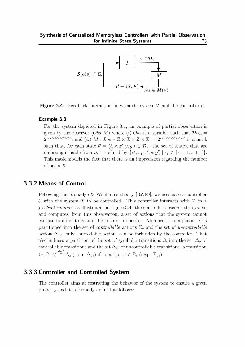
Synthesis of Centralized Memoryless Controllers with Partial Observationfor Infinite State Systems 73
T
C = 〈S, E〉
M
obs ∈M(ν)
ν ∈ DV
S(obs) ⊆ Σc
Figure 3.4 - Feedback interaction between the system T and the controller C.
Example 3.3
For the system depicted in Figure 3.1, an example of partial observation is
given by the observer 〈Obs,M〉 where (i) Obs is a variable such that DObs =
2Loc×Z×Z×Z×Z, and (ii) M : Loc × Z × Z × Z × Z → 2Loc×Z×Z×Z×Z is a mask
such that, for each state ~ν = 〈`, x, x′, y, y′〉 ∈ DV , the set of states, that are
undistinguishable from ~ν, is defined by {〈`, x1, x′, y, y′〉 |x1 ∈ [x − 1, x + 1]}.
This mask models the fact that there is an imprecision regarding the number
of parts X.
3.3.2 Means of Control
Following the Ramadge & Wonham’s theory [RW89], we associate a controller
C with the system T to be controlled. This controller interacts with T in a
feedback manner as illustrated in Figure 3.4: the controller observes the system
and computes, from this observation, a set of actions that the system cannot
execute in order to ensure the desired properties. Moreover, the alphabet Σ is
partitioned into the set of controllable actions Σc and the set of uncontrollable
actions Σuc; only controllable actions can be forbidden by the controller. That
also induces a partition of the set of symbolic transitions ∆ into the set ∆c of
controllable transitions and the set ∆uc of uncontrollable transitions: a transition
〈σ,G,A〉def∈ ∆c (resp. ∆uc) if its action σ ∈ Σc (resp. Σuc).
3.3.3 Controller and Controlled System
The controller aims at restricting the behavior of the system to ensure a given
property and it is formally defined as follows:

74 Chapter 3
Definition 3.9 (Controller)
Given an STS T = 〈V,Θ0,Θm,Σ,∆〉 and an observer 〈Obs,M〉, a controller
with partial observation for the system T is a pair C def= 〈S, E〉, where:
• S : DObs → 2Σc is a supervisory function which defines, for each obser-
vation obs ∈ DObs, a set S(obs) of controllable actions that are forbidden
when obs is observed by the controller.
• E ⊆ DV is a set of states which restricts the set of initial states of T .
This controller is memoryless, since its control decisions are only based on the
current observation received from the system. We recall that when the system
reaches a state ~ν ∈ DV , the controller receives, as information, an observation
obs ∈M(~ν).
The system resulting from the feedback interaction between the system Tand the controller C is called the controlled system and is defined by an STS
having an additional variable to represent the observations that the controller
receives from the system. It is formally defined as follows:
Definition 3.10 (Controlled System)
Given an STS T = 〈V,Θ0,Θm,Σ,∆〉, an observer 〈Obs,M〉, and a controller
C = 〈S, E〉, the system T controlled by C, denoted by T/C, is an STS including
observations which is defined by T/Cdef= 〈V/C, (Θ0)/C, (Θm)/C,Σ,∆/C〉, where:
• V/Cdef= V ·∪ 〈Obs〉 is a pair composed of the tuple of variables of V and
of the variable Obs.
• (Θ0)/Cdef= {〈~ν, obs〉 | (~ν ∈ (Θ0 \ E)) ∧ (obs ∈ M(~ν))} is the set of initial
states.
• (Θm)/Cdef= {〈~ν, obs〉 | (~ν ∈ Θm) ∧ (obs ∈ M(~ν))} is the set of marked
states.
• ∆/C is defined from ∆ as follows: for each transition 〈σ,G,A〉 ∈ ∆,
we define a new transition 〈σ,G/C, A/C〉def∈ ∆/C, where (i) G/C
def=
{〈~ν, obs〉 | (~ν ∈ G) ∧ (obs ∈ M(~ν)) ∧ (σ 6∈ S(obs))} and (ii) A/C is de-
fined, for each ~ν1 ∈ DV and for each obs1 ∈M(~ν1), by A/C(〈~ν1, obs1〉)def=
{〈~ν2, obs2〉|(~ν2 = A(~ν1)) ∧ (obs2 ∈M(~ν2))}.

Synthesis of Centralized Memoryless Controllers with Partial Observationfor Infinite State Systems 75
A state 〈~ν, obs〉 ∈ DV/C (with obs ∈ M(~ν)) of the controlled system models the
fact that when the system is in the state ~ν, the controller receives the observation
obs as information. The guards and the update functions of the controlled system
T/C are defined from the ones of the system T by taking into account the control
decisions of the controller C and the observations that it receives from the system:
• Guards: A transition 〈σ,G/C, A/C〉 ∈ ∆/C, defined from the transition
〈σ,G,A〉 ∈ ∆, can be fired from a state 〈~ν, obs〉 ∈ DV/C in the controlled
system if and only if (i) 〈σ,G,A〉 can be fired from ~ν in T , (ii) ~ν is compati-
ble with obs, and (iii) σ is not forbidden by the controller C in obs.
• Update functions: The update function A/C of the transition
〈σ,G/C, A/C〉 ∈ ∆/C, defined from the transition 〈σ,G,A〉 ∈ ∆, allows the
controlled system to reach the state 〈~ν2, obs2〉 ∈ DV/C from a 〈~ν1, obs1〉 ∈ DV/C
if and only if (i) the update function A allows the system to reach ~ν2 from
~ν1, and (ii) ~ν2 is compatible with obs2. These update functions A/C satisfy
the following property: (〈~ν2, obs2〉 ∈ A/C(〈~ν1, obs1〉)) ⇒ (∀obs3 ∈ M(~ν2) :
(〈~ν2, obs3〉 ∈ A/C(〈~ν1, obs1〉)). This property means that when the system
arrives in a state ~ν1, the controller can receive any observation of ~ν1.
3.3.4 Definition of the Control Problems
In this section, we are interested in three distinct versions of the state avoidance
control problem that consists in preventing the system from reaching some
particular states, either because some properties are not satisfied in these states
(e.g., the states where two state variables are equal or more generally the states
in which some particular state predicates are satisfied) or because they are
deadlocking or blocking states. We also prove some properties regarding these
problems.
Control Problems. The first problem is defined as follows:
Problem 3.1 (Basic State Avoidance Control Problem)
Given an STS T = 〈V,Θ0,Θm,Σ,∆〉, an observer 〈Obs,M〉 and a predi-
cate Bad, which represents a set of forbidden states, the basic state avoid-
ance control problem (basic problem for short) consists in computing a
controller C = 〈S, E〉 such that (i) ReachableT/C∆/C
((Θ0)/C) 6= ∅ and (ii)(Reachable
T/C∆/C
((Θ0)/C)⌋
[1]
)∩Bad = ∅.

76 Chapter 3
We recall (see section 1.1) that the projection ReachableT/C∆/C
((Θ0)/C)⌋
[1]=
{~ν | ∃〈~ν, obs〉 ∈ ReachableT/C∆/C
((Θ0)/C)}. Therefore, the basic problem consists
in synthesizing a controller which is (i) non-trivial (i.e., the behavior of the re-
sulting controlled system is not empty) and (ii) valid (i.e., it prevents the system
from reaching a forbidden state).
A solution to the basic problem does not ensure that the controlled system
is deadlock free (i.e., it is not ensured that the controlled system has always the
possibility to make a move) or non-blocking (i.e., it is not ensured that a marked
state can always be reached in the controlled system). Since most of the time
a deadlocking system or a blocking system cannot be tolerated, we extend our
problem to these cases:
Problem 3.2 (Deadlock Free State Avoidance Control Problem)
Given an STS T = 〈V,Θ0,Θm,Σ,∆〉, an observer 〈Obs,M〉 and a predi-
cate Bad, which represents a set of forbidden states, the deadlock free state
avoidance control problem (deadlock free problem for short) consists in com-
puting a controller C = 〈S, E〉 such that (i) ReachableT/C∆/C
((Θ0)/C) 6= ∅, (ii)(Reachable
T/C∆/C
((Θ0)/C)⌋
[1]
)∩Bad = ∅, and (iii) T/C is deadlock free.
In other words, the controller must be (i) non-trivial and (ii) valid, and (iii) it
must define a deadlock free controlled system.
Problem 3.3 (Non-blocking State Avoidance Control Problem)
Given an STS T = 〈V,Θ0,Θm,Σ,∆〉, an observer 〈Obs,M〉 and a predi-
cate Bad, which represents a set of forbidden states, the non-blocking state
avoidance control problem (non-blocking problem for short) consists in com-
puting a controller C = 〈S, E〉 such that (i) ReachableT/C∆/C
((Θ0)/C) 6= ∅, (ii)(Reachable
T/C∆/C
((Θ0)/C)⌋
[1]
)∩Bad = ∅, and (iii) T/C is non-blocking.
In other words, the controller must be (i) non-trivial and (ii) valid, and (iii) it
must define a non-blocking controlled system.
Maximal Controller. These problems can be solved by several controllers and
we would like to determine the best (or maximal) solutions. For that, let us
consider a relation �, which provides a comparison criterion among the con-
trollers. The concept of �-maximal controller then allows us then to define the
best solutions (w.r.t. the criterion �) to these problems:

Synthesis of Centralized Memoryless Controllers with Partial Observationfor Infinite State Systems 77
Definition 3.11 (�-Maximal Controller)
Given an STS T = 〈V,Θ0,Θm,Σ,∆〉, an observer 〈Obs,M〉 and a partial order
� defining a relation between the controllers, we say that a controller C1 is �-
maximal if and only if, for each controller C2, either C1 and C2 are incomparable
(w.r.t. the relation �), or C2 � C1.
In the literature, there exist several permissiveness criteria. We can, for example,
mention:
• the �`g criterion (resp. �`m criterion): if the language generated (resp.
marked) by the controlled system defined by the controller C1 is included
in the language generated (resp. marked) by the controlled system defined by
the controller C2, then C1 �`g C2 (resp. C1 �`m C2).
• the �s criterion: if, for each observation obs, the set of actions allowed by the
controller C1 in obs is included in the set of actions allowed by the controller
C2 in obs, then C1 �s C2.
• the �p criterion: if the set of reachable states in the controlled system defined
by the controller C1, is included in the set of reachable states in the controlled
system defined by the controller C2, then C1 �p C2.
In this thesis, we use the permissiveness criterion �p to compare the quality
of the different solutions of a problem. It is formally defined as follows:
Definition 3.12 (Permissiveness)
Given an STS T = 〈V,Θ0,Θm,Σ,∆〉 and an observer 〈Obs,M〉, a controller
C1 = 〈S1, E1〉 is more permissive than a controller C2 = 〈S2, E2〉 (denoted
by C2 �p C1) if and only if ReachableT/C2∆/C2
((Θ0)/C2) ⊆ ReachableT/C1∆/C1
((Θ0)/C1).
When the inclusion is strict, we say that C1 is strictly more permissive than C2(denoted by C2 ≺p C1).
Indeed, we are interested in the state avoidance control problem, where the aim
is to prevent the system from reaching a set Bad of forbidden states. The best
controller that can be computed is the one which allows the controlled system
to exactly reach the set of good states Badc (as a reminder, Badc = DV \Bad).When such a controller does not exist, we would like to compute a controller such
that the resulting controlled system achieves the largest possible subset of Badc.
Therefore, it is more appropriate to define our comparison criterion w.r.t. the
set of states that are reachable in the controlled system. We can also note that
78 Chapter 3
x1
x2
x3
x4
x5
x6
e
e
e
e
a
a
b
b
Bad = I(Bad)
Figure 3.5 - System with two �p-maximal controllers.
two controlled systems with the same set of reachable states can have different
enabled transitions7.
We have the following property:
Proposition 3.3
There does not always exist a unique �p-maximal controller solving the basic
(resp. deadlock free and non-blocking) problem.
Proof
We show that the system8depicted in Figure 3.5 admits two �p-maximal con-
trollers as solution. In this system, (i) the set of states X = {xi | i ∈ [1, 6]}, (ii)
the set of initial states X0 = {x1, x2}, (iii) the set of marked states Xm = X,
and (iv) all transitions are controllable.
Moreover, the set Bad = {x5, x6} (a bad state is represented by a square) and
the observer 〈Obs,M〉 is defined as follows: DObs = {obs1, obs2, obs3} and the
mask M is defined in the following way:
M(x) =
obs1 if x ∈ {x1, x4}obs2 if x ∈ {x2, x3}obs3 if x ∈ {x5, x6}
There are two �p-maximal controllers which solve the basic (resp. deadlock
free and non-blocking) problem:
7We could have used an extended definition of permissiveness where the inclusion of theactions, that can be fired from the reachable states, is also taken into account, when twocontrolled systems have the same set of reachable states.

Synthesis of Centralized Memoryless Controllers with Partial Observationfor Infinite State Systems 79
• the controller C1 which forbids the action a in obs1:
ReachableT/C1∆/C1
((Θ0)/C1) = {〈x1, obs1〉, 〈x2, obs2〉, 〈x4, obs1〉}.
• the controller C2 which forbids the action b in obs2:
ReachableT/C2∆/C2
((Θ0)/C2) = {〈x1, obs1〉, 〈x2, obs2〉, 〈x3, obs2〉}.
These controllers C1 and C2 are also maximal w.r.t. the �`g , �`m and �s criteria
and thus Proposition 3.3 also holds for the concepts of �`g , �`m and �s-maximal
controllers.
Undecidability Results. Now, we prove, for any notion of �-maximality,
that we cannot define, for the basic, deadlock free and non-blocking problems,
effective algorithms (i.e., which always terminate) which compute �-maximal
controllers. For that, we show that the related decision problems are undecidable
(see Proposition 3.8) and we use the four following results (Propositions 3.4, 3.5,
3.6 and 3.7):
Proposition 3.4 ([HMR05])
Given an STS T = 〈V,Θ0,Θm,Σ,∆〉 and a state ~ν ∈ DV , the reachability
decision problem, which consists in deciding if the state ~ν is reachable in T , is
undecidable.
Proposition 3.5
Given an STS T = 〈V,Θ0,Θm,Σ,∆〉, an observer 〈Obs,M〉 and a predicate
Bad, which represents a set of forbidden states, the basic decision problem,
which consists in deciding if there exists a controller solving the basic problem,
is undecidable.
Proof
The proof consists in a reduction from the reachability decision problem (see
Proposition 3.4) to the basic decision problem. For that, we build an instance
of the basic decision problem from an instance of the reachability decision
problem in such a way that there exists a controller solving the basic problem
if and only if the state ~ν is not reachable in the STS T .
8Automata are particular cases of STS. When the system to be controlled is sufficientlysimple, we represent it directly by the corresponding automaton.
80 Chapter 3
Polynomial transformation from the reachability decision problem
to the basic decision problem: Let T = 〈V,Θ0,Θm,Σ,∆〉 and ~ν ∈ DV
be the elements defining an instance of the reachability decision problem. The
instance of the basic decision problem is then defined by:
• the system T ′ = 〈V,Θ0,Θm,Σ,∆〉. All actions of Σ are uncontrollable.
• the observer 〈Obs,M〉 where Obs = V and M = IdDV.
• the set Bad = {~ν}
Correctness of the reduction: Since all actions are uncontrollable, the
only controller C, that can be defined, is the one which forbids no action and
this controller is valid if and only if ReachableT∆(Θ0)∩Bad = ∅. Therefore, there
exists a controller solving the basic problem if and only if ~ν 6∈ ReachableT∆(Θ0)
(i.e., ~ν is not reachable in T ).
Proposition 3.6
Given an STS T = 〈V,Θ0,Θm,Σ,∆〉, an observer 〈Obs,M〉 and a predicate
Bad, which represents a set of forbidden states, the deadlock free decision prob-
lem, which consists in deciding if there exists a controller solving the deadlock
free problem, is undecidable.
Proof
The proof consists in a reduction from the basic decision problem to the dead-
lock free decision problem. For that, we build an instance of the deadlock
free decision problem from an instance of the basic decision problem in such a
way that a controller C is a solution of the basic problem if and only if it is a
solution of the deadlock free problem.
Polynomial transformation from the basic decision problem to the
deadlock free decision problem: Let T = 〈V,Θ0,Θm,Σ,∆〉, 〈Obs,M〉and Bad be the elements defining an instance of the basic decision problem.
The instance of the deadlock free decision problem is then defined by T ′ =
〈V,Θ0,Θm,Σ′,∆′〉, 〈Obs,M〉 and Bad where:
• Σ′ = Σ ] {τ}. The new action τ does not belong to Σ and is uncontrol-
lable.
• ∆′ = ∆ ] {〈τ,TTDV, IdDV
〉}. This new transition can be fired from any
state ~ν ∈ DV and loops on ~ν.
Synthesis of Centralized Memoryless Controllers with Partial Observationfor Infinite State Systems 81
Correctness of the reduction: The system T ′ is deadlock free, because
the uncontrollable transition 〈τ,TTDV, IdDV
〉 can be fired from any state of this
system. Moreover, given a controller C, the controlled system T ′/C is always
deadlock free, because the transition 〈τ,TTDV, IdDV
〉 cannot be forbidden by
C. Therefore, a controller C is a solution of the deadlock free problem if and
only if it is a solution of the basic problem.
Proposition 3.7
Given an STS T = 〈V,Θ0,Θm,Σ,∆〉, an observer 〈Obs,M〉 and a predicate
Bad, which represents a set of forbidden states, the non-blocking decision prob-
lem, which consists in deciding if there exists a controller solving the non-
blocking problem, is undecidable.
Proof
The proof consists in a reduction from the basic decision problem to the non-
blocking decision problem. For that, we build an instance of the non-blocking
decision problem from an instance of the basic decision problem in such a way
that a controller C is a solution of the basic problem if and only if it is a
solution of the non-blocking problem.
Polynomial transformation from the basic decision problem to the
non-blocking decision problem: Let T = 〈V,Θ0,Θm,Σ,∆〉, 〈Obs,M〉and Bad be the elements defining an instance of the basic decision problem.
The instance of the non-blocking decision problem is then defined by T =
〈V,Θ0,Θ′m,Σ,∆〉, 〈Obs,M〉 and Bad where Θ′
m = DV .
Correctness of the reduction: The system T ′ is non-blocking, because
all states of T ′ are marked. Moreover, given a controller C, the controlled
system T ′/C is also non-blocking. Therefore, a controller C is a solution of the
non-blocking problem if and only if it is a solution of the basic problem.
With the previous three properties, we can prove the following result of unde-
cidability:
Proposition 3.8
Given an STS T = 〈V,Θ0,Θm,Σ,∆〉, an observer 〈Obs,M〉 and a predicate
Bad, which represents a set of forbidden states, the maximal basic (resp. dead-
lock free and non-blocking) decision problem, which consists in deciding if the
basic (resp. deadlock free and non-blocking) problem admits at least one �-
maximal controller as solution, is undecidable.

82 Chapter 3
Proof
The proof is straightforward from Propositions 3.5, 3.6 and 3.7.
To overcome this negative result, we propose an approach, based on abstract
interpretation, which approximates some computations to ensure the termination
of the algorithms. Our aim, in the next sections, is to prove that this approach
gives correct controllers and to experimentally show that these solutions are of
good quality.
3.4 Computation by Means of Abstract Interpretation of
a Memoryless Controller for the Basic Problem
In this section, we present our method, based on abstract interpretation, which
synthesizes memoryless controllers for the basic problem. First, in section 3.4.1,
we present a semi-algorithm (i.e., which does not always terminate) which com-
putes a memoryless controller for the basic problem. Next, in section 3.4.2, we
explain how to extend it to obtain, at the price of some overapproximations, an
effective algorithm (i.e., which always terminates). Finally, in section 3.4.3, we
theoretically evaluate the permissiveness of our solutions and we explain how it
can be improved.
3.4.1 Semi-algorithm for the Basic Problem
Our algorithm, which synthesizes controllers for the basic problem, is composed
of two parts:
• we compute, using a fixpoint equation, the set I(Bad) of states that can lead
to Bad by triggering only uncontrollable transitions.
• we forbid, in each state ~ν of the system, all controllable actions that can lead to
I(Bad) from this state. Moreover, to take into account the partial observation,
we must also forbid these actions in the states that are undistinguishable from
~ν.
These two steps are formalized as follows:

Synthesis of Centralized Memoryless Controllers with Partial Observationfor Infinite State Systems 83
Computation of I(Bad). The set I(Bad) of states leading uncontrol-
lably to Bad is given by CoreachT∆uc(Bad) which, as a reminder, is defined by
CoreachT∆uc(Bad) =
⋃n≥0(PreT∆uc
)n(Bad). This set of states cannot always be
computed, because the coreachability is undecidable in the model of STS, and,
in section 3.4.2, we will use abstract interpretation techniques to overapproxi-
mate it. However, to compute this overapproximation, we must characterize the
set I(Bad) by a fixpoint equation. This equation is defined as follows over the
complete lattice 〈2DV ,⊆,∪,∩,DV , ∅〉:
I(Bad)def= lfp⊆(λB.Bad ∪ PreT∆uc
(B)) (3.1)
Since the function λB.Bad∪PreT∆uc(B) is monotonic, the Knaster-Tarski’s theo-
rem [Tar55] ensures that the least fixpoint of this function exists and the follow-
ing proposition proves that this fixpoint equation gives the set of states leading
uncontrollably to Bad:
Proposition 3.9
The function λB.Bad ∪ PreT∆uc(B) defined over the complete lattice 〈2DV ,⊆
,∪,∩,DV , ∅〉 is such that lfp⊆(λB.Bad ∪ PreT∆uc(B)) =
⋃n≥0(PreT∆uc
)n(Bad).
Proof
By the Knaster-Tarski and Kleene’s theorems, it suffices to show that the
function PreT∆ucis continuous to prove this proposition. We must thus prove
that, for each increasing sequence of sets B1 ⊆ B2 ⊆ . . . ⊆ Bn ⊆ . . . (where
∀i ≥ 1 : Bi ∈ 2DV ), the equality PreT∆uc(⋃
i≥1Bi) =⋃
i≥1 PreT∆uc(Bi) holds.
For that, we first prove that, for each δ = 〈σ,G,A〉 ∈ ∆, PreTδ (⋃
i≥1Bi) =⋃i≥1 PreTδ (Bi):
PreTδ
(⋃i≥1
Bi
)= G ∩ A−1
(⋃i≥1
Bi
), by definition of PreTδ
= G ∩
(⋃i≥1
A−1(Bi)
), because the function A−1 is
continuous by assumption.
=⋃i≥1
(G ∩ A−1(Bi)), because a ∩
(⋃i
bi
)=⋃i
(a ∩ bi).
=⋃i≥1
PreTδ (Bi)

84 Chapter 3
B
obs1
obs2
!ν1!ν3
!ν4
σ1
σ2!ν2
Figure 3.6 - Computation of F(σi, B) (for i = 1, 2).
Next, we prove that, for each D ⊆ ∆, PreTD(⋃
i≥1Bi) =⋃
i≥1 PreTD(Bi):
PreTD
(⋃i≥1
Bi
)=
⋃δ∈D
PreTδ
(⋃i≥1
Bi
), by definition of PreTD
=⋃δ∈D
(⋃i≥1
PreTδ (Bi)
), because PreTδ is continuous.
=⋃i≥1
(⋃δ∈D
PreTδ (Bi)
)=
⋃i≥1
PreTD(Bi)
Computation of the Controller C. To compute this controller, we first define
the function F : Σ × 2DV → 2DObs which gives, for each action σ ∈ Σ and set
B ⊆ DV of states to be forbidden, the set F(σ,B) of observations, in which the
action σ must be forbidden. More precisely, this set F(σ,B) corresponds to the
greatest set O of observations such that, for each observation obs ∈ O, there

Synthesis of Centralized Memoryless Controllers with Partial Observationfor Infinite State Systems 85
exists a state ~ν ∈ DV which is compatible with obs and which leads to B by a
transition labeled by σ:
F(σ,B)def=
{M(PreTσ (B) \B) if σ ∈ Σc
∅ otherwise(3.2)
Example 3.4
Figure 3.6 illustrates this computation. Let us suppose that ~ν1 leads to B by
the controllable action σ1 and that ~ν2 leads to B by the controllable action
σ2. The observations obs1, obs2 ∈ F(σ1, B), because ~ν1 is compatible with obs1
and obs2, and the observation obs2 ∈ F(σ2, B), because ~ν2 is compatible with
obs2.
Next, the controller C is defined in the following way:
C def= 〈S, E〉 (3.3)
with the elements S and E defined as follows:
• the supervisory function S is given, for each observation obs ∈ DObs, by:
S(obs)def= {σ ∈ Σc | obs ∈ F(σ, I(Bad))} (3.4)
It means that σ is forbidden in obs if I(Bad) is reachable from a state com-
patible with obs by a transition labeled by σ.
• the set Edef= I(Bad). It prevents the controlled system from beginning its
execution in a state which can lead to Bad by a sequence of uncontrollable
transitions.
The set I(Bad) and the function F are computed offline. Next, during the
execution of the system, when the controller receives an observation obs ∈ DObs,
it computes online the set S(obs) of actions to be forbidden (the computation
of this set is based on the function F). Since Σ is finite, S(obs) is computable
when I(Bad) is computed.
Example 3.5
For the system depicted in Figure 3.1, the controller must ensure, during the
phase of consumption of the parts X, the presence of a minimal number of
parts of this kind: Bad = {〈CX, x, x′, y, y′〉 | (x ≤ 1000) ∧ (y ∈ [0, 2])}.

86 Chapter 3
The controller has a partial observation of the system, which is modeled by
the mask M defined in Example 3.3 i.e., for each state ~ν = 〈`, x, x′, y, y′〉 ∈DV , the set of states which are undistinguishable from ~ν, is given by
{〈`, x1, x′, y, y′〉 |x1 ∈ [x − 1, x + 1]}. The controllable (resp. uncontrollable)
transitions are drawn in plain (resp. dashed) lines. The computation of the
set I(Bad) gives:
I(Bad) = Bad ∪ {〈CX, x, x′, y, y′〉 | [(x ≤ 1001) ∧ (y ∈ [1, 2])] ∨[(x ≤ 1002) ∧ (y = 2)]}
and the computation of the function F gives:
F(σ, I(Bad)) =
{M({〈PX, x, x′, y, y′〉 |x ≤ 1002}) if σ = Stop prod
∅ otherwise
Therefore, the supervisory function S forbids the action Stop prod when the
system is in a state ~ν ∈ {〈PX, x, x′, y, y′〉 |x ≤ 1003} and it forbids no action
in the other states of the system. One can note that the controller computed
for this system is �p-maximal.
The following property proves that our algorithm synthesizes correct controllers
for the basic problem:
Proposition 3.10
Given an STS T = 〈V,Θ0,Θm,Σ,∆〉, an observer 〈Obs,M〉 and a predicate
Bad, which represents a set of forbidden states, the controller C = 〈S, E〉,defined by (3.3), solves the basic problem (when Θ0 6⊆ E).
Proof
We prove by induction on the length n of the sequences of transitions (these se-
quences begin in an initial state) that(Reachable
T/C∆/C
((Θ0)/C)⌋
[1]
)∩I(Bad) = ∅.
Since Bad ⊆ I(Bad), this property implies that(Reachable
T/C∆/C
((Θ0)/C)⌋
[1]
)∩
Bad = ∅.
• Base case (n = 0): the execution of the controlled system T/C starts in
a state which does not belong to I(Bad), since (Θ0)/C⌋
[1]= Θ0 \ E =
Θ0 \ I(Bad).

Synthesis of Centralized Memoryless Controllers with Partial Observationfor Infinite State Systems 87
• Induction step: we suppose that the proposition holds for the sequences
of transitions of length less than or equal to n and we prove that this
property remains true for the sequences of transitions of length n+1. By
induction hypothesis, each state ~ν1 reachable by a sequence of transitions
of length n does not belong to I(Bad) and we show that each transition
δ = 〈σ,G,A〉 ∈ ∆, which can lead to a state ~ν2 ∈ I(Bad) from this state
~ν1 in the system T , cannot be fired from ~ν1 in the controlled system T/C.
For that, we consider two cases :
• if δ ∈ ∆c, then this transition cannot be fired from ~ν1 in the system
T/C, since σ ∈ S(obs) (∀obs ∈M(~ν1)) by (3.2) and (3.4).
• if δ ∈ ∆uc, then ~ν2 ∈ I(Bad) (by (3.1)), which is impossible by
hypothesis.
Hence, in the controlled system, the forbidden state ~ν2 cannot be reached
from the state ~ν1 by the transition δ.
The feedback interaction between a system T = 〈V,Θ0,Θm,Σ,∆〉 to be con-
trolled and a controller C (see Figure 3.4) gives the controlled system T/C =
〈V/C, (Θ0)/C, (Θm)/C,Σ,∆/C〉 given in Definition 3.10. In some cases, it can be in-
teresting to compute this controlled system. Unfortunately, when the mask M is
a covering of the state space this controlled system cannot always be computed.
Indeed, in our tool, we perform the computations by manipulating symbolically
sets of states to avoid enumerating these sets. But, this approach cannot be used
to compute the transitions 〈σ,G/C, A/C〉 (defined from 〈σ,G,A〉) of the controlled
system, because the computation of G/C requires to associate the observations
of M(~ν), which are not forbidden by the controller, with each state ~ν ∈ G. Ob-
viously, this enumeration is not always possible, because the state space can be
infinite.
However, when the mask M corresponds to a partition of the state space,
the definition of the controlled system is simplified (the observations can be
omitted in the definition, because each state has exactly an observation), which
makes possible its computation. Indeed, the simplified definition of the controlled
system is the following:

88 Chapter 3
Definition 3.13 (Controlled System when the Mask is a Partition)
Given an STS T = 〈V,Θ0,Θm,Σ,∆〉, an observer 〈Obs,M〉 (where M cor-
responds to a partition of DV ), and a controller C = 〈S, E〉, the sys-
tem T controlled by C, denoted by T/C, is an STS defined by T/Cdef=
〈V, (Θ0)/C,Θm,Σ,∆/C〉, where:
• (Θ0)/Cdef= {~ν |~ν ∈ (Θ0 \ E)} is the set of initial states.
• ∆/C is defined from ∆ as follows: for each transition 〈σ,G,A〉 ∈ ∆,
we define a new transition 〈σ,G/C, A〉def∈ ∆/C, where G/C
def= {~ν | (~ν ∈
G) ∧ (σ 6∈ S(M(~ν)))}.
This controlled system T/C = 〈V, (Θ0)/C,Θm,Σ,∆/C〉 can be computed for our
controller C = 〈S, I(Bad)〉 (defined by (3.3)) since (i) (Θ0)/C is obtained by
computing the set operation Θ0 \ I(Bad) and (ii) the restricted guard G/C of
any transition 〈σ,G/C, A〉 ∈ ∆/C (defined from the transition 〈σ,G,A〉 ∈ ∆) is
obtained by computing the set operation G \ {M−1(F(σ, I(Bad)))}.
3.4.2 Effective Algorithm for the Basic Problem
The algorithm described in the previous section requires to compute the fixpoint
I(Bad), but this equation cannot always be computed for undecidability (or
complexity) reasons. We overcome this obstacle by using abstract interpretation
techniques (see e.g. [CC77, HPR97, Jea03]) in order to compute an overapprox-
imation of the fixpoint I(Bad) in a finite time. Since our algorithm then uses
an overapproximation of I(Bad), the synthesized controllers remain correct, but
they can be less permissive.
We use abstract interpretation by means of the representation framework
(see section 1.4.2) instead of the Galois connection framework (see section 1.4.1),
because the abstract lattice that we use (i.e., the lattice of convex polyhedra) is
not complete. The lattice of convex polyhedra constitutes one of the most used
abstract lattice and it has been used successfully in many applications (e.g., for
the analysis and verification of linear hybrid automata [HHWt97], for detecting
buffer overflows in C [DRS01],. . . ). We define the elements which constitute the
representation framework as follows.
Definition of the Elements of the Representation Framework. The con-

Synthesis of Centralized Memoryless Controllers with Partial Observationfor Infinite State Systems 89
crete lattice is defined by the 6-tuples 〈2DV ,⊆,∪,∩,DV , ∅〉 (as a reminder, the
tuple V gives the variables of the system to be controlled) and the used repre-
sentation (see Definition 1.18) is defined by the 3-tuple 〈〈Λ,v,t,u,>,⊥〉, γ,∇〉.(i) The abstract lattice 〈Λ,v,t,u,>,⊥〉 corresponds to the lattice of convex
polyhedra; the concepts of convex polyhedron and of lattice of convex polyhedra
are defined as follows:
Definition 3.14 (Convex Polyhedron)
A convex polyhedron on the tuple of variables V = 〈v1, . . . , vn〉 is defined by a
conjunction of k linear constraints∧
1≤i≤k ai,1.v1 + . . .+ ai,n.vn ≤ ci, where (i)
ai,1, . . . , ai,n ∈ Q (∀i ∈ [1, k]) are coefficients and (ii) ci ∈ Q (∀i ∈ [1, n]) is a
constant.
Definition 3.15 (Lattice of Convex Polyhedra)
The lattice of convex polyhedra is defined by the 6-tuples 〈Λ,v,t,u,>,⊥〉where:
• Λ is the set of convex polyhedra on the tuple of variables V .
• the v operator is defined by the classical set inclusion operator.
• the t operator of two convex polyhedra P1 and P2 is defined by the con-
vex hull of P1 and P2, which gives the least convex polyhedron containing
both P1 and P2. The convex hull is used as an overapproximation of the
set union, because this operation is not closed for convex polyhedra.
• the u operator of two convex polyhedra is defined by the classical set
intersection operator. This operation is closed for convex polyhedra.
• > is defined by the convex polyhedron which represents the entire state
space.
• ⊥ is the empty set.
(ii) The concretization function γ : Λ→ 2DV is defined by the identity function.
(iii) The widening operator ∇ is the standard widening defined in [CH78]. The
widening of two convex polyhedra P1 and P2 (denoted by P1∇P2) such that
P1 v P2 consists in removing from P1 all constraints which are not satisfied by
P2. In other words, if between P1 and P2 the value of a variable or a linear
expression grows, then the widening operator considers that it grows indefinitely

90 Chapter 3
x
y
1 20
1
P1
P2
(a) Convex polyhedra P1 and P2.
x
y
1 20
1
P1 ! P2
P1 ! P2
(b) Convex polyhedra P1 u P2 and P1 t P2.
Figure 3.7 - An example of u and t operations.
and thus it removes it.
To correctly perform the computations in the abstract lattice, each element
B ⊆ DV of the concrete lattice must safely be transposed into an element α(B) of
the abstract lattice i.e., B ⊆ γ(α(B)) (see Definition 1.18). For that, we use the
abstraction function α : 2DV → Λ defined as follows: for each set B ∈ 2DV , if B
corresponds to a polyhedron, then α(B) is defined by the least convex polyhedron
which contains B, otherwise α(B) is defined by >. In this definition, we consider
two cases to transpose the elements of the concrete lattice, because when B is
not a polyhedron, the least convex polyhedron containing B does not always
exist (e.g., when B represents a circle). The abstraction of the elements, which
do not correspond to polyhedra, is rough, but this definition of α is satisfactory
for our tool, because we only need to abstract polyhedra.
Example 3.6
Let us consider a state space with two integer variables x and y. The convex
polyhedron P1 = (x ≥ 0) ∧ (y ≥ 0) ∧ (x+ y ≤ 1) defines a right-angle triangle
and the convex polyhedron P2 = (x ≥ 0.5)∧ (x ≤ 2)∧ (y ≥ 0)∧ (y ≤ 1) defines
a rectangle (see Figure 3.7(a)).
The intersection of P1 and P2 gives the convex polyhedron P3 = (x ≥ 0.5) ∧(y ≥ 0) ∧ (x + y ≤ 1) (see Figure 3.7(b)) and the convex hull of P1 and P2
gives the convex polyhedron P4 = (x ≥ 0) ∧ (x ≤ 2) ∧ (y ≥ 0) ∧ (y ≤ 1) (see
Figure 3.7(b)).

Synthesis of Centralized Memoryless Controllers with Partial Observationfor Infinite State Systems 91
x
y
10
1
P1P3
(a) Convex polyhedra P1 and P3.
x
y
10
1
P3∇P1
(b) Convex polyhedron P3∇P1.
Figure 3.8 - An example of widening operations.
The widening operation P3∇P1 gives the convex polyhedron P5 = (y ≥ 0) ∧(x + y ≤ 1), because P1 does not satisfy the linear constraint x ≥ 0.5 (see
Figure 3.8(b)).
Effective Algorithm for the Basic Problem. The effective algorithm is quite
similar to the semi-algorithm defined in section 3.4.1: the main differences are
that we perform the computations in the abstract lattice and that we compute
an overapproximation of I(Bad) to ensure the termination of our algorithm.
More precisely, to compute this overapproximation, we use Theorem 1.4 with
the instantiation of the representation framework defined above. This theorem
requires to transpose the functions used in the computation of I(Bad) into the
abstract lattice. First, we perform this transposition for the function PreTD :
2DV → 2DV (where D ⊆ ∆) and we obtain the function PreT ,]D : Λ→ Λ which is
defined, for each ` ∈ Λ, by:
PreT ,]D (`)
def=⊔δ∈D
PreT ,]δ (`) , where (3.5)
PreT ,]δ (`)
def= α(Gδ ∩ A−1
δ (γ(`))) (3.6)
Next, we transpose the fixpoint equation I(Bad) into the abstract lattice and we
obtain:
I](Bad)def= lfpv(λ`.α(Bad) t PreT ,]
∆uc(`)) (3.7)
According to Theorem 1.4, we compute the element a∞ defined as the limit of
92 Chapter 3
the following sequence:
ai =
{⊥ if i = 0
ai−1∇(α(Bad) t PreT ,]∆uc
(ai−1)) if i > 0(3.8)
Theorem 1.4 ensures that this element a∞ is obtained after a finite number of
steps and that a∞ is a post-fixpoint of I](Bad). Moreover, it ensures that γ(a∞) is
a post-fixpoint of I(Bad). Therefore, I ′(Bad) = γ(a∞) is an overapproximation
of I(Bad) (one can note that γ(a∞) = a∞, because γ is the identity function).
Note that we can use this theorem, because all constraints that it requires are
fulfilled.
After computing the overapproximation of I(Bad), we transpose the control
function F into the abstract lattice and we obtain the abstract function F ].
The computation of the control function may thus require overapproximations.
Finally, we define our controller C = 〈S, I ′(Bad)〉 as in (3.3) by using I ′(Bad)
and F ] instead of I(Bad) and F . The controller, that we obtain, is correct,
because I ′(Bad) ⊇ I(Bad). It is worthy notable that the obtained controller can
make unreachable more states than necessary, then it can be less permissive.
In general, a variant of the fixpoint computation strategy described in (3.8) is
used to compute an overapproximation of the least fixpoint of a function. Indeed,
in this strategy the widening operator is applied at each iteration, which can give
rough results. Abstract interpretation theory suggests to wait several iterations
before using for the first time the widening operator and to separate two succes-
sive applications of the widening operator from several iterations. In our tool,
we use the fixpoint computation strategy defined in [Bou92] and based on these
recommendations. This strategy is parametrized by three elements ki, ks and kr.
Parameter ki gives the iteration at which the widening operator must be used
for the first time and ks gives the number of iterations between two successive
applications of the widening operator. Therefore, the widening operator is used
at the iterations ki + j.ks (∀j ≥ 0); otherwise, we use the t. Moreover, a post-
fixpoint of a function can be refined by applying this function to this element and
the parameter kr specifies the number of times that this operation must be per-
formed. Increasing the value of the parameters ki, ks and kr generally improves
the quality of the overapproximations, but the time complexity to compute them
also increases. A trade-off between these two aspects must thus be found. This
compromise depends on the considered function, the used representation and the
user requirements. In our tool, we use small values for the parameters ki, ks and
kr (in general, ki, ks, kr ∈ [1, 10]) and we obtain good results with these values.

Synthesis of Centralized Memoryless Controllers with Partial Observationfor Infinite State Systems 93
x
y
0
100
1000 1001
a1
1
(a) Computation of a1.
x
y
0
100
1000 1001
Bad ! PreT ,!∆ (a1)
1
(b) Computation of Bad t PreT ,]∆ (a1).
x
y
0
100
1000 1001
a2
1
(c) Computation of a2.
Figure 3.9 - An example of fixpoint computations with the strategy described
in (3.8).

94 Chapter 3
x
y
0
100
1000 1001
a1
1
1100
(a) Computation of a1.
x
y
0
100
1000 1001
a2
1
1100
(b) Computation of a2.
x
y
0
100
1000 1001
a3
1
1100
(c) Computation of a3.
Figure 3.10 - An example of fixpoint computations with the strategy used in
our tool.

Synthesis of Centralized Memoryless Controllers with Partial Observationfor Infinite State Systems 95
Example 3.7
Let us illustrate the effective algorithm by considering the system depicted
in Figure 3.1, where the transitions δ1 and δ4 are respectively replaced by
〈Cons; 0 ≤ y ≤ 100;x := x − 1, y := y − 1〉 and 〈Stop prod; TTDV; y := 100〉.
The set Bad of forbidden states is defined by {〈CX, x, x′, y, y′〉 | (x ≤ 1000) ∧(y ∈ [0, 100])} and the controller has a full observation of the system.
If we use the fixpoint computation strategy described in (3.8) to compute an
overapproximation of I(Bad), we obtain the following sequence of values for
the variables x, x′, y, y′ in the location CX (see Figure 3.9): (i) a0 = ⊥, (ii)
a1 = ⊥∇((x ≤ 1000)∧(y ≥ 0)∧(y ≤ 100)) = (x ≤ 1000)∧(y ≥ 0)∧(y ≤ 100),
(iii) a2 = a1∇((x ≤ 1001) ∧ (y ≥ 0) ∧ (y ≤ 100) ∧ (x − y ≤ 1000)) = (y ≥0) ∧ (y ≤ 100). Thus, I ′(Bad) = {〈CX, x, x′, y, y′〉 | (y ≤ 100) ∧ (y ≥ 0)} and
the controller always forbids the action Stop prod in the location PX.
If we use the fixpoint computation strategy of our tool with ki = ks = kr = 3,
we obtain the following sequence of values for the x, x′, y, y′ in the location CX
(see Figure 3.10): (i) a0 = ⊥, (ii) a1 = ⊥t((x ≤ 1000)∧(y ≥ 0)∧(y ≤ 100)) =
(x ≤ 1000) ∧ (y ≥ 0) ∧ (y ≤ 100), (iii) a2 = a1 t ((x ≤ 1001) ∧ (y ≥ 0) ∧ (y ≤100)∧(x−y ≤ 1000)) = (x ≤ 1001)∧(y ≥ 0)∧(y ≤ 100)∧(x−y ≤ 1000), (iv)
a3 = a2∇((x ≤ 1002)∧ (y ≥ 0)∧ (y ≤ 100)∧ (x− y ≤ 1000)) = (y ≥ 0)∧ (y ≤100)∧(x−y ≤ 1000). In this example, the refinement (parameter kr) of a3 does
not modify the value of this element. Thus, I ′(Bad) = {〈CX, x, x′, y, y′〉 | (y ≤100)∧(y ≥ 0)∧(x−y ≤ 1000)} and the controller forbids the action Stop prod
in the location PX when x ≤ 1100. One can note that this controller is �p-
maximal.
Quality of the Approximations. The method presented in this section always
computes a correct controller, but it does not guarantee that this controller is
�p-maximal. The quality of this controller depends on the overapproximation
of I(Bad) that we compute. We must thus compute good approximations and
there are classical techniques to improve the quality of these approximations:
• the choice of the abstract lattice is the main issue. If it is not adapted to
the kind of guards or assignments of the STS, the overapproximations are too
rough. The practice shows that if the guards are linear constraints, and if the
assignment functions are also linear, the lattice, that we use (i.e., the lattice
of convex polyhedra [CH78]), gives good results.
• the computation of the fixpoint with the widening operator is also an impor-
tant issue and it can be improved by several ways: (i) we can use a more

96 Chapter 3
x
y
P2P1
R1 = R2
(a) P1 v R1 and P2 v R2.
x
y
P1∇P2
R1∇R2
(b) P1∇P2 6v R1∇R2.
Figure 3.11 - An example which illustrates that using a more precise abstract
lattice does not always give better results for the widening.
elaborate widening, like the widening up to, instead of the standard widen-
ing [HPR97], (ii) we can use one of the fixpoint computation strategies defined
in [Bou92], (iii) we can refine our abstract lattice (see [Jea03] for more details),
and (iv) we can refine the post-fixpoint obtained with the widening operator
by using a narrowing operator [CC77]. Roughly, this operation consists in
computing a decreasing sequence of post-fixpoints (where the first element is
the post-fixpoint computed with the widening operator) in order to improve
the overapproximation of the least fixpoint.
In the literature, there are few theoretical results on the quality of abstractions.
This lack of results is mainly due to the fact that the widening operator is not
monotonic. Indeed, because of this property, an improvement in the elements
used in the abstractions does not necessarily imply that the iterative fixpoint
computation gives a more precise overapproximation. Therefore, it is difficult to
theoretically evaluate the quality of abstractions.

Synthesis of Centralized Memoryless Controllers with Partial Observationfor Infinite State Systems 97
Example 3.8
This example illustrates that using a more precise abstract lattice to represent
sets of states does not always give better results in an iterative fixpoint com-
putation. Let us suppose that two sets of states are represented on one hand
by the convex polyhedra P1 and P2 and on the other hand by the rectangles
R1 and R2 with P1 v R1 and P2 v R2 (see Figure 3.11). P1 and P2 are thus
more precise than R1 and R2, but P1∇P2 is not more precise than R1∇R2.
Since it is difficult to theoretically analyze the quality of abstractions, we
have implemented our algorithm to evaluate it experimentally. The results are
available in section 3.7.
3.4.3 Evaluation and Improvement of the Permissiveness of the Con-
troller
In this section, we compare the permissiveness of our control algorithm with the
one of an algorithm defined in the literature [TK98] and we explain how we can
modify our algorithm to improve its permissiveness.
Evaluation of the Permissiveness in the Finite Case. To the best of
our knowledge, there is no control algorithm which synthesizes controllers with
partial observation for the basic problem in the case of infinite state systems.
Therefore, we restrict our attention to the case of finite state systems and the
most permissive controller, that we found, is the one defined by Takai et al.
in [TK98] (they assume that the masks are partitions of the state space). The
following proposition shows that our algorithm and the one defined in [TK98]
have the same permissiveness:
Proposition 3.11
When the basic problem is restricted to the case where the system to be
controlled is finite and the mask is a partition of the state space, the controller
defined in (3.3) and the one defined in [TK98] have the same permissiveness.
Proof
First, we outline the work defined in [TK98]. The authors propose an algorithm
solving the basic problem where (i) the system to be controlled is modeled
by a finite deterministic automaton T = 〈X, x0, Xm,Σ,∆〉, (ii) the control
specification is given by a set Q ⊆ X of good states (i.e., Q = X \Bad), and
98 Chapter 3
(iii) the partial observation is modeled by a mask M : X → DObs correspond-
ing to a partition of X. This algorithm is composed of two steps:
• the computation of the set of safe states Q↑ ⊆ Q where Q↑ def=⋂∞
j=0Qj,
with Qj defined recursively as follows:
Qjdef=
{Q if j = 0
g(Qj−1) otherwise
where, for each Q′ ⊆ Q, the function g(Q′)def= Q ∩
(⋂σ∈Σuc
{x1 ∈X | ∀x2 ∈ X : (〈x1, σ, x2〉 ∈ ∆)⇒ (x2 ∈ Q′)}
).
• the computation of the control function f , which gives the actions that
are allowed by the controller and which is defined, for each obs ∈ DObs,
by f(obs)def= Σ \ {σ ∈ Σc | ∃x1 ∈ Q↑,∃x2 6∈ Q↑ : (obs = M(x1)) ∧
(〈x1, σ, x2〉 ∈ ∆)}.
Since the system is finite and the function g is monotonic, all computations
terminate in a finite amount of time; in particular, there exists an integer n
such that Q↑ =⋂n
j=0Qj.
We remark that Q↑ = (I(Bad))c, because we can prove by induction that
∀j ≥ 0 :⋂
i≤j Qi = (⋃
i≤j(PreTΣuc)i(Bad))c. Moreover, to prevent from reaching
I(Bad), our supervisory function S forbids, for each observation obs ∈ DObs,
the set of actions S(obs) = {σ ∈ Σc|∃x1 6∈ I(Bad),∃x2 ∈ I(Bad) : (M(x1) =
obs)∧ (〈x1, σ, x2〉 ∈ ∆)}. Therefore, we have that f(obs) = Σ\S(obs), for each
obs ∈ DObs.
Improvement of the Permissiveness. Now, we explain how to improve the
computation of our supervisory function S, defined in (3.4), in order to obtain
a more permissive controller C acting on infinite state systems to be controlled.
This improvement is based on the observations done in the following example.
Example 3.9
In the system depicted in Figure 3.12, (i) the set of states X = {xi | i ∈ [1, 7]},(ii) the set of initial states X0 = {x1, x2}, (iii) the set of final states Xm = X,
and (iv) all transitions are controllable.
Moreover, the set Bad = {x5, x6} and the observer 〈Obs,M〉 is defined as
follows: DObs = {obs1, obs2, obs3} and the mask M is defined in the following
way:

Synthesis of Centralized Memoryless Controllers with Partial Observationfor Infinite State Systems 99
x1
x2
x3
x4
x7
a
bca
e
b
x5
x6
Bad = I(Bad)
Figure 3.12 - Improvement of the control algorithm.
M(x) =
obs1 if x ∈ {x1, x4, x7}obs2 if x ∈ {x2, x3}obs3 if x ∈ {x5, x6}
(3.9)
Our controller C forbids the action b in the observation obs2 and the action a
in the observation obs1. However, it is sufficient to forbid b in obs2, because
the state x4 is then no longer reachable and this controller is strictly more
permissive than C, because it allows the system to reach x7.
We remark that when we forbid an action σ, some actions σ′ can no more be
fired in the system since they can only be fired from states that are no longer
reachable. Our improved algorithm, which computes a controller for the basic
problem, is based on this remark.
The idea of this algorithm is to choose an action σ ∈ Σ, that leads to I(Bad)
from a state which is not in I(Bad), and to forbid this action. This operation
is repeated while the set I(Bad) is reachable in the current controlled system.
The performance of this algorithm depends on the choice of the action σ to be
forbidden. Roughly, our heuristic consists in choosing an action σ such that the
controlled system, which is obtained, maximizes the states in (I(Bad))c and
minimizes the states in I(Bad). The main difference with the algorithm defined
in section 3.4.1 is that we verify that an action can still be fired in the current
controlled system, before deciding to forbid it or not. Our algorithm is composed
of three subalgorithms: (i) getController (main algorithm), (ii) actionToForbid
(called by getController) and (iii) getMax (called by actionToForbid).
Algorithm 1 (main algorithm). This algorithm computes a controller solving the

100 Chapter 3
basic problem. For that, it calls Algorithm 2, which chooses an action σ to be
forbidden. Next, it computes the set F(σ, I(Bad)) of observations in which the
action σ must be forbidden (this computation is based on (3.2)). Then, the su-
pervisory function S and the controller C are modified to take into account the
change of F . These operations are repeated while I(Bad) is reachable in the con-
trolled system. This algorithm requires to compute the set ReachableT/C∆/C
((Θ0)/C)
(see line 7) of states that are reachable in the controlled system T/C. Therefore, to
be able to compute this controlled system T/C, we consider masks corresponding
to partitions of the state space.
Algorithm 1: getController(T , 〈Obs,M〉, Bad)input : An STS T = 〈V,Θ0,Θm,Σ,∆〉, an observer 〈Obs, M〉 (with M corresponding
to a partition of the state space) and a set of forbidden states Bad.output: Either a controller C solving the basic problem, or NIL when the algorithm
does not find a solution to this problem.begin1
∀obs ∈ DObs, S(obs)← ∅ \\S forbids no action.2
C ← 〈S, I(Bad)〉 \\ C is defined by S and I(Bad).3
if (Θ0)/C ⊆ I(Bad) then4
\\ The controller C is trivial5
return (NIL)6
while ReachableT/C∆/C
((Θ0)/C) ∩ I(Bad) 6= ∅ do7
\\ The algorithm continues while I(Bad) is reachable.8
σ ← actionToForbid(T , 〈Obs, M〉, Bad,F , C)\\ Algorithm 2 chooses the action to be forbidden.9
F(σ, I(Bad))←M(PreT/Cσ (I(Bad)) \ I(Bad))10
\\ Computation of the observations in which σ must be forbidden.11
∀obs ∈ DObs, S(obs)← {σ ∈ Σc | obs ∈ F(σ, I(Bad))}12
\\ S is modified to take into account the change of F .13
C ← 〈S, I(Bad)〉 \\ C is defined by S and I(Bad).14
return (C)15
end16
Algorithm 2. This algorithm selects an action σ that the controller C in
construction must forbid. For that, Algorithm 2 considers all actions σ1 that
can potentially be forbidden by this controller i.e., all actions that can be fired
in the controlled system, that can lead to a forbidden state, and that have not
been chosen by this algorithm in a previous call (see line 3). Next, it computes,
for each of these actions σ1, the set of states that would be reachable if the
controller C (in construction) forbids σ1 (see line 10) and it uses Algorithm 3,
which is based on this reachability information, to obtain the best (w.r.t. our
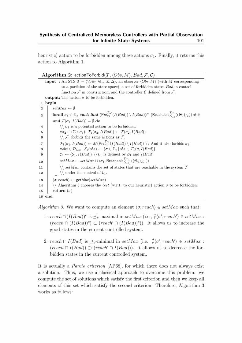
Synthesis of Centralized Memoryless Controllers with Partial Observationfor Infinite State Systems 101
heuristic) action to be forbidden among these actions σ1. Finally, it returns this
action to Algorithm 1.
Algorithm 2: actionToForbid(T , 〈Obs,M〉, Bad,F , C)input : An STS T = 〈V,Θ0,Θm,Σ,∆〉, an observer 〈Obs, M〉 (with M corresponding
to a partition of the state space), a set of forbidden states Bad, a controlfunction F in construction, and the controller C defined from F .
output: The action σ to be forbidden.begin1
setMax← ∅2
forall σ1 ∈ Σc such that (PreT/Cσ1 (I(Bad)) \ I(Bad))∩ (Reachable
T/C∆/C
((Θ0)/C)) 6= ∅3
and F(σ1, I(Bad)) = ∅ do\\ σ1 is a potential action to be forbidden.4
∀σ2 ∈ (Σ \ σ1), F1(σ2, I(Bad))← F(σ2, I(Bad))5
\\ F1 forbids the same actions as F .6
F1(σ1, I(Bad))←M(PreT/Cσ1 (I(Bad)) \ I(Bad)) \\ And it also forbids σ1.7
∀obs ∈ DObs, S1(obs)← {σ ∈ Σc | obs ∈ F1(σ, I(Bad)}8
C1 ← 〈S1, I(Bad)〉 \\ C1 is defined by S1 and I(Bad).9
setMax← setMax ∪ 〈σ1,ReachableT/C1∆/C1
((Θ0)/C1)〉10
\\ setMax contains the set of states that are reachable in the system T11
\\ under the control of C1.12
〈σ, reach〉 ← getMax(setMax)13
\\ Algorithm 3 chooses the best (w.r.t. to our heuristic) action σ to be forbidden.14
return (σ)15
end16
Algorithm 3. We want to compute an element 〈σ, reach〉 ∈ setMax such that:
1. reach∩ (I(Bad))c is �p-maximal in setMax (i.e., @〈σ′, reach′〉 ∈ setMax :
(reach ∩ (I(Bad))c) ⊂ (reach′ ∩ (I(Bad))c)). It allows us to increase the
good states in the current controlled system.
2. reach ∩ I(Bad) is �p-minimal in setMax (i.e., @〈σ′, reach′〉 ∈ setMax :
(reach ∩ I(Bad)) ⊃ (reach′ ∩ I(Bad))). It allows us to decrease the for-
bidden states in the current controlled system.
It is actually a Pareto criterion [AP68], for which there does not always exist
a solution. Thus, we use a classical approach to overcome this problem: we
compute the set of solutions which satisfy the first criterion and then we keep all
elements of this set which satisfy the second criterion. Therefore, Algorithm 3
works as follows:

102 Chapter 3
• it computes the set setMax1, which contains the elements 〈σ1, reach1〉 ∈setMax, that satisfy the following condition (denoted by Cond.(i) in the se-
quel): reach1 ∩ (I(Bad))c is �p-maximal in setMax (i.e., @〈σ2, reach2〉 ∈setMax : (reach1 ∩ (I(Bad))c) ⊂ (reach2 ∩ (I(Bad))c)).
• it computes the set setMax2, which contains the elements 〈σ1, reach1〉 ∈setMax1, that satisfy the following condition (denoted by Cond.(ii) in the
sequel): reach1 ∩ I(Bad) is �p-minimal in setMax1 (i.e. @〈σ2, reach2〉 ∈setMax1 : (reach1 ∩ I(Bad)) ⊃ (reach2 ∩ I(Bad))).
• it non-deterministically chooses an element of setMax2 and returns this value.
Algorithm 3: getMax(setMax)
input : A set setMax of pairs 〈σ, reach〉.output: An element 〈σ, reach〉 ∈ setMax which satisfies Cond.(i) and Cond.(ii) (see
the explanations of this algorithm).begin1
setMax1 ← {〈σ1, reach1〉 ∈ setMax|@〈σ2, reach2〉 ∈ setMax :2
((reach1 ∩ (I(Bad))c) ⊂ (reach2 ∩ (I(Bad))c))}\\ Contains the elements 〈σ1, reach1〉 ∈ setMax such that reach1 ∩ (I(Bad))c is3
\\ �p-maximal (Cond.(i)).4
setMax2 ← {〈σ1, reach1〉 ∈ setMax1|@〈σ2, reach2〉 ∈ setMax1 :5
(reach1 ∩ I(Bad)) ⊃ (reach2 ∩ I(Bad))}\\ Contains the elements 〈σ1, reach1〉 ∈ setMax1 such that reach1 ∩ I(Bad) is6
\\ �p-minimal (Cond.(ii)).7
Chooses an element 〈σ, reach〉 of setMax2 non-deterministically8
return (〈σ, reach〉)9
end10
Algorithm 1 computes non-trivial and valid controllers for the basic problem
(due to lines 4 and 7 of Algorithm 1). Moreover, this algorithm outperforms
or gives, at least, the same result as the controller defined in (3.3), because the
following property always holds: ∀obs ∈ DObs,S ′(obs) ⊆ S(obs) (where S ′ is the
supervisory function computed by Algorithm 1 and S is the supervisory function
of the controller defined in (3.3)).
To ensure the termination of Algorithm 1, we use abstract interpretation
techniques as in section 3.4.2. More precisely, we transpose the computations
into the abstract lattice and perform them in this simpler lattice. Moreover, to
ensure the convergence in the computation of the function ReachableT/C∆/C
((Θ0)/C)
(see line 7 of Algorithm 1 and lines 3 and 10 of Algorithm 2), we proceed similarly
to the method defined for the function Coreach described in section 3.4.2. As
explained above, these computations may require overapproximations.

Synthesis of Centralized Memoryless Controllers with Partial Observationfor Infinite State Systems 103
3.5 Computation by Means of Abstract Interpretation
of a Memoryless Controller for the Deadlock Free
Problem
So far we have been interested in computing controllers solving the basic problem.
But a solution to this problem does not ensure that the controlled system has the
possibility to fire a transition in each reachable state. Since, most of the time,
a deadlocking system is not tolerated, we extend, in this section, the method
defined in section 3.4 in order to synthesize controllers for the deadlock free
problem.
First, in section 3.5.1, we present a semi-algorithm which computes a mem-
oryless controller for the deadlock free problem, and then, in section 3.5.2, we
explain how to extend it to obtain, at the price of some overapproximations, an
effective algorithm.
3.5.1 Semi-algorithm for the Deadlock Free Problem
Our algorithm, which synthesizes controllers for the deadlock free problem, is
composed of two parts: (i) first, we compute, using a fixpoint equation, the set
Idf (Bad) of states that can lead to Bad or to deadlocking states by triggering
only uncontrollable transitions and (ii) then, we forbid all controllable actions
that can lead to a state of the set Idf (Bad) (this part is similar to the one
defined for the basic problem). Before formalizing these two steps, we explain
how to compute the deadlocking states:
Computation of the Deadlocking States. Computing Idf (Bad) requires to
compute the states that would be in deadlock after control. Note that if a state
〈~ν, obs1〉 (with obs1 ∈ M(~ν)) of the controlled system is in deadlock, then the
states 〈~ν, obs2〉 (∀obs2 ∈M(~ν)) must also be forbidden, because when the system
arrives in the state ~ν, the controller non-deterministically receives an observation
of the setM(~ν). So, when we give the deadlocking states of the controlled system,
we can omit the observations. Hence, we define a function PreTdf : 2DV → 2DV
which gives, for each set B ⊆ DV of states to be forbidden, the set PreTdf (B) of
states that would be in deadlock in the controlled system which avoids B. Since
we cannot compute the controlled system (when the mask is a covering of the
state space), we must define these deadlocking states of the controlled system
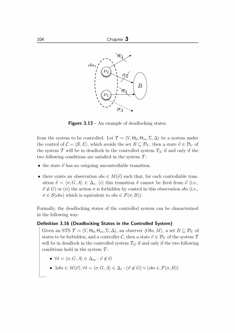
104 Chapter 3
obs1
B
σ2
σ1
σ1
σ3
ν1
ν2
Figure 3.13 - An example of deadlocking states.
from the system to be controlled. Let T = 〈V,Θ0,Θm,Σ,∆〉 be a system under
the control of C = 〈S, E〉, which avoids the set B ⊆ DV , then a state ~ν ∈ DV of
the system T will be in deadlock in the controlled system T/C if and only if the
two following conditions are satisfied in the system T :
• the state ~ν has no outgoing uncontrollable transition.
• there exists an observation obs ∈ M(~ν) such that, for each controllable tran-
sition δ = 〈σ,G,A〉 ∈ ∆c, (i) this transition δ cannot be fired from ~ν (i.e.,
~ν 6∈ G) or (ii) the action σ is forbidden by control in this observation obs (i.e.,
σ ∈ S(obs) which is equivalent to obs ∈ F(σ,B)).
Formally, the deadlocking states of the controlled system can be characterized
in the following way:
Definition 3.16 (Deadlocking States in the Controlled System)
Given an STS T = 〈V,Θ0,Θm,Σ,∆〉, an observer 〈Obs,M〉, a set B ⊆ DV of
states to be forbidden, and a controller C, then a state ~ν ∈ DV of the system Twill be in deadlock in the controlled system T/C if and only if the two following
conditions hold in the system T :
• ∀δ = 〈σ,G,A〉 ∈ ∆uc : ~ν 6∈ G
• ∃obs ∈M(~ν),∀δ = 〈σ,G,A〉 ∈ ∆c : (~ν 6∈ G) ∨ (obs ∈ F(σ,B))
Synthesis of Centralized Memoryless Controllers with Partial Observationfor Infinite State Systems 105
Example 3.10
The system depicted in Figure 3.13 illustrates the definition of deadlocking
states. In this system, the states ~ν1 and ~ν2 are compatible with the observation
obs1. The state ~ν1 is deadlock free, because the uncontrollable action σ3 can
always be fired and the state ~ν2 is in deadlock, because no action can be fired
from this state. Indeed, the action σ1 is forbidden in obs1, because this action
leads to B from ~ν1 and the action σ2 is forbidden in obs1, because its leads to
B from ~ν2.
However, we have two remarks regarding the computation of the deadlocking
states (i.e., the function PreTdf ) defined in Definition 3.16:
1. The function PreTdf will be used to define the fixpoint equation Idf (Bad)
(see (3.12)). By the Knaster-Tarski theorem [Tar55], if the function PreTdfis monotonic, then it is ensured that the fixpoint equation Idf (Bad) admits
a solution. However, the computation of the deadlocking states depends
on the function F (see Definition 3.16) which is not monotonic. Therefore,
in the sequel, we will use the monotonic function F instead of F in the
computation of these states:
F(σ,B) =
{M(PreTσ (B)) if σ ∈ Σc
∅ otherwise(3.10)
One can note that the function F is rougher than F .
2. Computing all states, that will be in deadlock in the controlled system,
is not possible with our symbolic operations. Indeed, for the second con-
dition of Definition 3.16, we must combine, for each controllable transi-
tion 〈σ,G,A〉, the set of states Gc and the set of observations F(σ,B),
but the domains of these sets are different. If we transform F(σ,B) into
M−1(F(σ,B)), we no longer know in which observations the action σ has
been forbidden. However, we need this information, because we have an
existential quantification on the observations in the second condition of
Definition 3.16. If we transform Gc into M(Gc), then there can be states
in M−1(M(Gc)) from which δ can be fired.
To overcome the second remark, we will consider the subcase9 where the mask
M is a partition of the state space. Indeed, in this case, each state ~ν ∈ DV
9In [KLMM10], we have shown that the deadlocking states can also be computed in thesubcase where M is a covering and the observation space DObs is finite.
106 Chapter 3
is compatible with exactly one observation, which simplifies the definition of
deadlocking states and makes possible the computation of these elements:
Definition 3.17 (Deadlocking States when M is a partition)
Given an STS T = 〈V,Θ0,Θm,Σ,∆〉, an observer 〈Obs,M〉 (where M corre-
sponds to a partition of the state space), a setB ⊆ DV of states to be forbidden,
and a controller C, then a state ~ν ∈ DV of the system T will be in deadlock in
the controlled system T/C if and only if the two following conditions10 hold in
the system T :
• ∀δ = 〈σ,G,A〉 ∈ ∆uc : ~ν 6∈ G
• ∀δ = 〈σ,G,A〉 ∈ ∆c : (~ν 6∈ G) ∨ (~ν ∈M−1(F(σ,B)))
A state ~ν is in deadlock if it has no outgoing uncontrollable transition and if its
outgoing controllable transitions δ = 〈σ,G,A〉 are forbidden by control in the
observation M(~ν) (i.e., σ ∈ S(M(~ν)) which is equivalent to ~ν ∈M−1(F(σ,B))).
Since, for each σ ∈ Σuc, the set F(σ,B) = ∅, the function PreTdf (B) (with B ⊆DV ), which gives the set of states, that would be in deadlock in the controlled
system avoiding B, can be expressed as follows:
PreTdf (B) = B ∪
[ ⋂〈σ,G,A〉∈∆
(Gc ∪ (M−1(F(σ,B)))
)](3.11)
Now that we have a function (see (3.11)) computing the deadlocking states,
we formalize the two steps of our algorithm defined for the deadlock free problem:
Computation of Idf(Bad). The set Idf (Bad) corresponds to the set of states
leading uncontrollably to a forbidden state or to a deadlocking state. To compute
Idf (Bad), we first compute the set I(Bad) (defined in (3.1)). Then, if we make
unreachable these forbidden states by cutting all controllable transitions that lead
to a bad state, the corresponding controlled system could have new deadlocking
states. These states are given by the function PreTdf (I(Bad)) and we add them
to the set of forbidden states. Adding these deadlocking states to the set of
forbidden states can provide new states leading uncontrollably to a forbidden
state. Consequently, the set Idf (Bad) is defined by⋃
n≥0(PreTdf ◦ I)n(Bad). This
10We assume that M−1(∅) = ∅.

Synthesis of Centralized Memoryless Controllers with Partial Observationfor Infinite State Systems 107
set of states cannot always be computed, because the coreachability is undecidable
in the model of STS, and, in section 3.5.2, we will use abstract interpretation
techniques to overapproximate it. However, to compute this overapproximation,
we must characterize the set Idf (Bad) by a fixpoint equation. This equation is
defined as follows over the complete lattice 〈2DV ,⊆,∪,∩,DV , ∅〉:
Idf (Bad)def= lfp⊆(λB.Bad ∪ PreTdf (I(B))) (3.12)
Since the function λB.Bad∪PreTdf (I(B)) is monotonic, the Knaster-Tarski’s the-
orem [Tar55] ensures that the least fixpoint of this function exists and the follow-
ing proposition proves that this fixpoint equation gives the set of states leading
uncontrollably to a forbidden state or to a deadlocking state:
Proposition 3.12
The function λB.Bad ∪ PreTdf (I(B)) defined over the complete lattice 〈2DV ,⊆,∪,∩,DV , ∅〉 is such that lfp⊆(λB.Bad∪PreTdf (I(B))) =
⋃n≥0(PreTdf ◦I)n(Bad).
Proof
By the Knaster-Tarski and Kleene’s theorems, it suffices to show that the
functions I and PreTdf are continuous to prove this proposition. In Propo-
sition 3.9, we have already proven that the function I is continuous. For
the second function, we must prove that, for each increasing sequence of
sets B1 ⊆ B2 ⊆ . . . ⊆ Bn ⊆ . . . (where ∀i ≥ 1 : Bi ∈ 2DV ), the equality
PreTdf (⋃
i≥1Bi) =⋃
i≥1 PreTdf (Bi) holds. This equality is proved by the follow-
ing reasoning, where a transition δ ∈ ∆ is defined by the triple 〈σ,G,A〉:
PreTdf
(⋃i≥1
Bi
)
=
(⋃i≥1
Bi
)∪
[ ⋂δ∈∆
(Gc ∪ (M−1(F(σ,
⋃i≥1
Bi)))
)], by
definition of PreTdf .
=
(⋃i≥1
Bi
)∪
[ ⋂δ∈∆
(Gc ∪ [M−1(M(PreTσ
(⋃i≥1
Bi
)))]
)],
by definition of F .

108 Chapter 3
=
(⋃i≥1
Bi
)∪
[ ⋂δ∈∆
[Gc ∪
[⋃i≥1
(M−1(M(PreTσ (Bi))))
]]],
because PreTσ = PreTTrans(σ) is continuous (see Proof of
Proposition 3.9) and because M and M−1 are
continuous.
=
(⋃i≥1
Bi
)∪
[ ⋂δ∈∆
[⋃i≥1
(Gc ∪ [M−1(M(PreTσ (Bi)))]
)]],
because a ∪
(⋃i
bi
)=⋃i
(a ∪ bi).
=
(⋃i≥1
Bi
)∪
[⋃i≥1
[ ⋂δ∈∆
(Gc ∪ [M−1(M(PreTσ (Bi)))]
)]],
because ∆ is finite and a ∩
(⋃i
bi
)=⋃i
(a ∩ bi).
=⋃i≥1
(Bi ∪
[ ⋂δ∈∆
(Gc ∪ [M−1(M(PreTσ (Bi)))]
)])=
⋃i≥1
PreTdf (Bi)
Computation of the Controller C. The controller C is defined as in sec-
tion 3.4.1 (see (3.3)) by using Idf (Bad) instead of I(Bad). More precisely, the
controller C is defined by the pair 〈S, Idf (Bad)〉 where the supervisory function Sis defined as in (3.4) by using the function F(σ, Idf (Bad)) instead of F(σ, I(Bad))
(∀σ ∈ Σ).
Example 3.11
For the system depicted in Figure 3.1, the controller must prevent the
system from reaching the set Bad = {〈CX, x, x′, y, y′〉 | (x ≤ 0) ∧ (y ∈[0, 2])} ∪ {〈PX, x, x′, y, y′〉 |x ≥ 6}. The controller has a partial observa-
tion of the system, which is modeled by the mask M where, for each state
~ν = 〈`, x, x′, y, y′〉 ∈ DV :

Synthesis of Centralized Memoryless Controllers with Partial Observationfor Infinite State Systems 109
• if x ≥ 2, then the controller cannot distinguish ~ν from the states in the
set {〈`, x1, x′, y, y′〉 |x1 ≥ 2},
• if x < 2, then the controller perfectly observes this state.
The computation of the set I(Bad) gives:
I(Bad) = Bad ∪ {〈CX, x, x′, y, y′〉 | [(x ≤ 1) ∧ (y ∈ [1, 2])] ∨ [(x ≤ 2)
∧(y = 2)]}
and the computation of the function F gives:
F(σ, I(Bad)) =
M({〈PX, x, x′, y, y′〉 |x ≤ 2}) if σ = Stop prod
M({〈PX, x, x′, y, y′〉 |x ≥ 5}) if σ = Prod
M({〈Choice, x, x′, y, y′〉 |x ≥ 6}) if σ = Choice X
∅ otherwise
Therefore, to prevent the system from reaching I(Bad), the controller for-
bids (i) the action Stop prod when the system is in the location PX, (ii)
the action Prod when the system is in a state ~ν ∈ {〈PX, x, x′, y, y′〉 |x ≥2}, and (iii) the action Choice X when the system is in a state ~ν ∈{〈Choice, x, x′, y, y′〉 |x ≥ 2}. Since the states ~ν ∈ {〈PX, x, x′, y, y′〉 |x ≥ 2}are in deadlock, they are added to the forbidden states i.e., PreTdf (I(Bad)) =
I(Bad) ∪ {〈PX, x, x′, y, y′〉 |x ≥ 2}. The set of states I(PreTdf (I(Bad))) =
PreTdf (I(Bad)). Consequently, to prevent the system from reaching these
states, the controller forbids (i) the action Stop prod when the system is
in the location PX, (ii) the action Prod when the system is in a state
~ν ∈ {〈PX, x, x′, y, y′〉 |x ≥ 1}, and (iii) the action Choice X when the
system is in a state ~ν ∈ {〈Choice, x, x′, y, y′〉 |x ≥ 2}. Since the states
~ν ∈ {〈PX, x, x′, y, y′〉 |x ≥ 1} are in deadlock, they are added to the for-
bidden states. By continuing the computations in this way, we obtain (i) a
set Idf (Bad) = I(Bad) ∪ {〈PX, x, x′, y, y′〉 |x, x′, y, y′ ∈ Z} and (ii) a control
function F defined by:
F(σ, Idf (Bad)) =
M({〈Choice, x, x′, y, y′〉 |x, x′, y, y′ ∈ Z})
if σ = Choice X
∅ otherwise
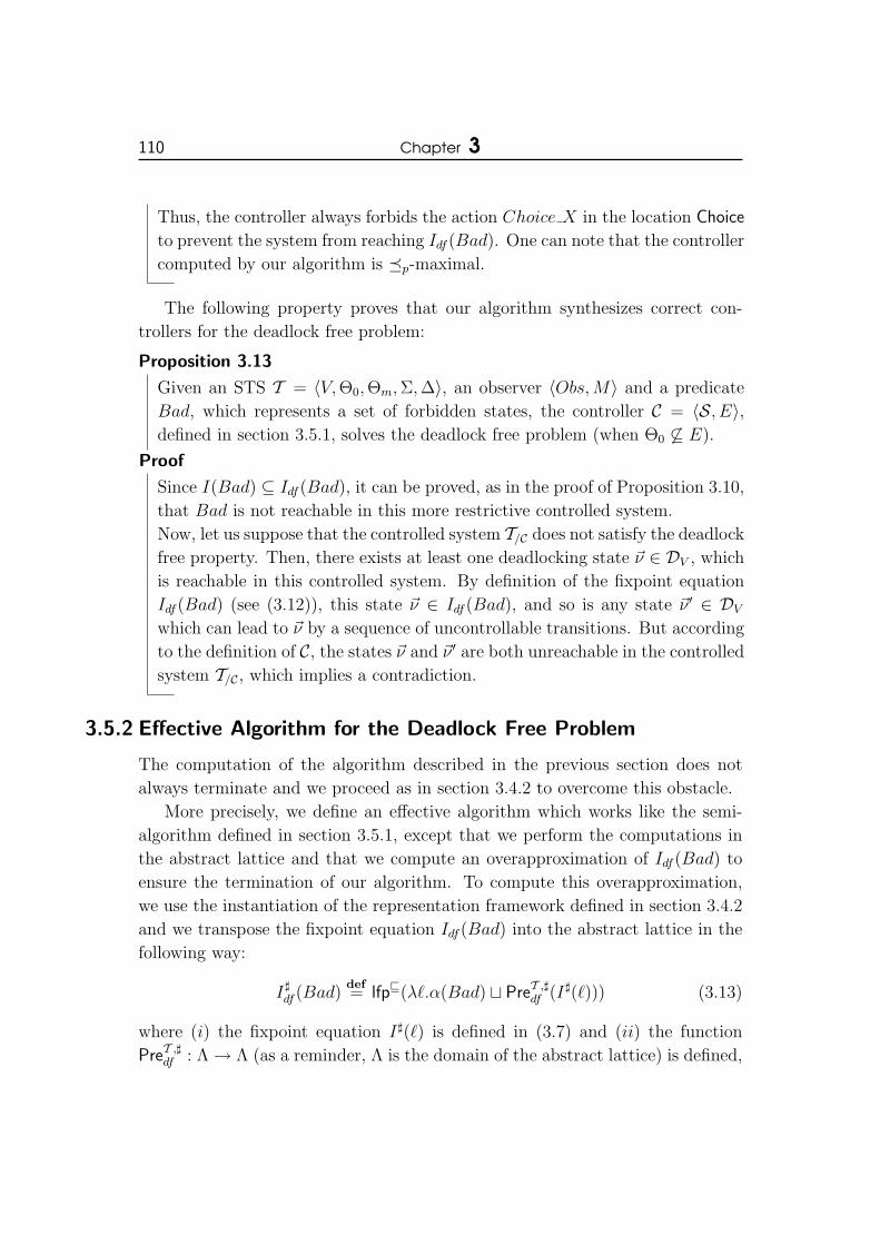
110 Chapter 3
Thus, the controller always forbids the action Choice X in the location Choice
to prevent the system from reaching Idf (Bad). One can note that the controller
computed by our algorithm is �p-maximal.
The following property proves that our algorithm synthesizes correct con-
trollers for the deadlock free problem:
Proposition 3.13
Given an STS T = 〈V,Θ0,Θm,Σ,∆〉, an observer 〈Obs,M〉 and a predicate
Bad, which represents a set of forbidden states, the controller C = 〈S, E〉,defined in section 3.5.1, solves the deadlock free problem (when Θ0 6⊆ E).
Proof
Since I(Bad) ⊆ Idf (Bad), it can be proved, as in the proof of Proposition 3.10,
that Bad is not reachable in this more restrictive controlled system.
Now, let us suppose that the controlled system T/C does not satisfy the deadlock
free property. Then, there exists at least one deadlocking state ~ν ∈ DV , which
is reachable in this controlled system. By definition of the fixpoint equation
Idf (Bad) (see (3.12)), this state ~ν ∈ Idf (Bad), and so is any state ~ν ′ ∈ DV
which can lead to ~ν by a sequence of uncontrollable transitions. But according
to the definition of C, the states ~ν and ~ν ′ are both unreachable in the controlled
system T/C, which implies a contradiction.
3.5.2 Effective Algorithm for the Deadlock Free Problem
The computation of the algorithm described in the previous section does not
always terminate and we proceed as in section 3.4.2 to overcome this obstacle.
More precisely, we define an effective algorithm which works like the semi-
algorithm defined in section 3.5.1, except that we perform the computations in
the abstract lattice and that we compute an overapproximation of Idf (Bad) to
ensure the termination of our algorithm. To compute this overapproximation,
we use the instantiation of the representation framework defined in section 3.4.2
and we transpose the fixpoint equation Idf (Bad) into the abstract lattice in the
following way:
I]df (Bad)
def= lfpv(λ`.α(Bad) t PreT ,]
df (I](`))) (3.13)
where (i) the fixpoint equation I](`) is defined in (3.7) and (ii) the function
PreT ,]df : Λ→ Λ (as a reminder, Λ is the domain of the abstract lattice) is defined,

Synthesis of Centralized Memoryless Controllers with Partial Observationfor Infinite State Systems 111
for each ` ∈ Λ, by:
PreT ,]df (`)
def= ` t
[l
〈σ,G,A〉∈∆
[α(Gc) t
(α(M−1(M(γ(PreT ,]
Trans(σ)(`))))))]]
(3.14)
where PreT ,]Trans(σ)(`) is defined in (3.5).
Next, we use the fixpoint computation strategy defined in section 3.4.2 to
compute a post-fixpoint a∞ of I]df (Bad) and the element γ(a∞) (denoted by
I ′df (Bad)) gives an overapproximation of Idf (Bad).
Then, we transpose the control function F into the abstract lattice and we ob-
tain the abstract function F ]. Finally, we define our controller C = 〈S, I ′df (Bad)〉as in (3.3) by using I ′df (Bad) and F ].
3.6 The Non-blocking Problem
The computation of controllers for the non-blocking problem is interesting, but
our approach, based on the computation of safe approximations, cannot effica-
ciously be applied to this problem. Indeed, let us suppose that we adapt our
approach, defined for the deadlock free problem, to the non-blocking problem
by computing the set Ibl(Bad) of states that can lead to Bad or to blocking
states by triggering only uncontrollable transitions. The set of blocking states
of a system T can then be obtained by computing the complement of the set
of non-blocking states, which is given by CoreachT∆(Θm). Since the computation
of CoreachT∆(Θm) does not always terminate, we can use abstract interpretation
techniques to compute an overapproximation of this set. However, we then ob-
tain an underapproximation of the blocking states and hence the controllers that
we compute are not correct. To obtain correct controllers, we must compute an
underapproximation of CoreachT∆(Θm), but the computation of such approxima-
tions with abstract interpretation do not generally give good results.
3.7 Experimental Results
The algorithms presented in the previous sections have been implemented in our
tool SMACS (Symbolic MAsked Controller Synthesis) in order to evaluate our
approach experimentally. In section 3.7.1, we briefly describe our tool (a more
detailed description of SMACS and an explanation of our implementation choices

112 Chapter 3
are given in appendix A) and, in section 3.7.2, we present several examples and
describe the solutions computed by SMACS.
3.7.1 Description of SMACS
The input of SMACS is a description of the STS to be controlled (we consider
STS with explicit locations) and the variables of this system can be of two types:
integer and real. The guards of the transitions are boolean combinations of
linear constraints and the assignments are given by linear expressions. The set
of forbidden states is specified by a boolean combination of linear constraints
and the masks can be of four kinds:
• Undistinguishable locations: the controller cannot distinguish some given
locations of the system.
• Hidden variables: the controller has no information regarding the value of
some given variables.
• Partially hidden variables: the value of a numerical variable is unknown
when it belongs to a given interval (the user can specify an interval for each
variable).
• Undistinguishable intervals: when the system is in a state ~ν =
〈ν1, . . . , νn〉 ∈ DV , the controller cannot distinguish this state from the states
in the set {〈ν ′1, . . . , ν ′n〉 ∈ DV | ∀i ∈ [1, n] : ν ′i ∈ [νi−ci, νi+c′i]}, where ci, c
′i ∈ R
(∀i ∈ [1, n]) are constants. One can note that ci and c′i can be different from
cj and c′j (∀i 6= j ∈ [1, n]).
The first three masks are partitions of the state space and the last one is a
covering. If no mask is specified, the controller has a full observation of the
system.
The output of SMACS is a description of the function F : it displays, for each
action σ, the set of observations in which σ is forbidden. Moreover, SMACS
computes and displays (graphically) the controlled system for the first three
masks.
SMACS allows the use of three abstract lattices: the lattice of intervals, the
lattice of octagons and the lattice of convex polyhedra. The lattice of intervals
and the lattice of convex polyhedra have respectively been defined in section 1.4.1
and in Definition 3.15. The lattice of octagons can be seen as a particular case
of the lattice of convex polyhedra where the coefficients ai,j (for each i ∈ [1, k]
and for each j ∈ [1, n]), used in Definition 3.14, are equal to 1.

Synthesis of Centralized Memoryless Controllers with Partial Observationfor Infinite State Systems 113
δ2 = 〈u1;TTDV ;x := y − 5〉
δ3 = 〈c0;TTDV ;x := 4 ∗ x〉
δ8 = 〈u1;x ≤ 1000;x := x− 1〉
δ9 = 〈u0;x = 10; IdDV 〉
δ7 = 〈c0;x ≤ y; IdDV 〉
δ4 = 〈c2;TTDV ; y := x + 2〉
δ5 = 〈c3;TTDV ;x := x + 1〉
δ1 = 〈c2;TTDV ; IdDV 〉
δ10 = 〈u1;TTDV ;x := y; y := x〉 δ11 = 〈c1;TTDV ;x := 5; y := 2〉
δ12 = 〈u0;TTDV ;x := 2 ∗ y + 4〉
δ6 = 〈c3;TTDV ; y := y + 2〉
!0 !1
!2
!3 !4!5
!6
!7!8
Figure 3.14 - Toy example.
3.7.2 Empirical Evaluation
We consider several examples and present the solutions computed by SMACS in
order to evaluate our approach experimentally. Our experiments are performed
with several abstract lattices.
Toy Example. The first system to be controlled is depicted in Figure 3.14.
This STS has a tuple V = 〈`, x, y〉 of three variables, where (i) ` ∈ {`i | i ∈ [0, 8]}gives the current location of the system, and (ii) x, y ∈ Z. The initial state is
〈`0, 0, 0〉 and the set Bad of forbidden states is defined by {〈`6, x, y〉|x, y ∈ Z}.We consider several cases that are summarized in Table 3.1:
(i) The controller does not ensure the deadlock free property and it has a
full observation of the system. With the lattices of convex polyhedra and
octagons, SMACS computes a set I(Bad) = Bad ∪ {〈`2, x, y〉 | 10 ≤ x ≤1000}. Next, SMACS forbids the action c0 in the location `3 when (10 ≤x ≤ 1000) ∧ (y ≥ x) to prevent the system from reaching I(Bad). The
graphical output of the controlled system generated by SMACS is given in
Figure 3.15. With the lattice of intervals, the control is more restrictive:

114 Chapter 3
l8
l0
[u1]
( #true ) {y = x,x = y}
l7
[u0]
( #true ) {x = ((2. * y) + 4.)}
l6
l5
l3
[c2]
( #true ) {y = (x + 2.)}
l4
[c0]
( #true ) {x = (4. * x)}
l2
[c0]
( (x<=y) AND NOT ((((1000. + (-1. * x)) + (0. * y))>=0.) AND ((0. + (-1. * x)) + (1. * y)) >=0.) AND ((-10. + (1. * x)) + (0. * y)) >=0.] )
{}
[c3]
( #true ) {y = (y + 2.)}
[u0]
( x == 10. ) {}
[u1]
( x <= 1000. ) {x = (x - 1.)}
l1
[u1]
( #true ) {x = (y - 5.)}
[c1]
( #true ) {y = 2.,x = 5.}
[c3]
( #true ) {x = (x + 1.)}
[c2]
( #true ) {}
Figure 3.15 - Controlled system generated by SMACS for the toy example when
the controller has a full observation of the system and when the
deadlock free property is not ensured.
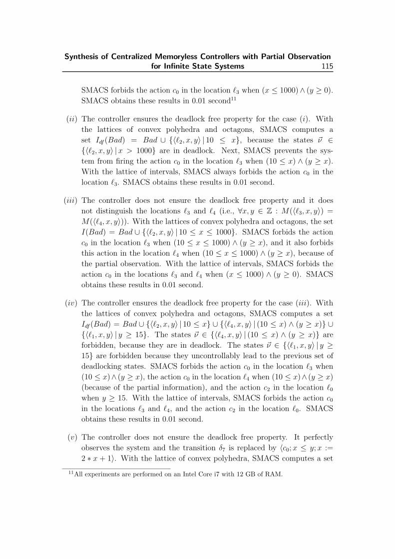
Synthesis of Centralized Memoryless Controllers with Partial Observationfor Infinite State Systems 115
SMACS forbids the action c0 in the location `3 when (x ≤ 1000)∧ (y ≥ 0).
SMACS obtains these results in 0.01 second11
(ii) The controller ensures the deadlock free property for the case (i). With
the lattices of convex polyhedra and octagons, SMACS computes a
set Idf (Bad) = Bad ∪ {〈`2, x, y〉 | 10 ≤ x}, because the states ~ν ∈{〈`2, x, y〉 |x > 1000} are in deadlock. Next, SMACS prevents the sys-
tem from firing the action c0 in the location `3 when (10 ≤ x) ∧ (y ≥ x).
With the lattice of intervals, SMACS always forbids the action c0 in the
location `3. SMACS obtains these results in 0.01 second.
(iii) The controller does not ensure the deadlock free property and it does
not distinguish the locations `3 and `4 (i.e., ∀x, y ∈ Z : M(〈`3, x, y〉) =
M(〈`4, x, y〉)). With the lattices of convex polyhedra and octagons, the set
I(Bad) = Bad ∪ {〈`2, x, y〉 | 10 ≤ x ≤ 1000}. SMACS forbids the action
c0 in the location `3 when (10 ≤ x ≤ 1000) ∧ (y ≥ x), and it also forbids
this action in the location `4 when (10 ≤ x ≤ 1000) ∧ (y ≥ x), because of
the partial observation. With the lattice of intervals, SMACS forbids the
action c0 in the locations `3 and `4 when (x ≤ 1000) ∧ (y ≥ 0). SMACS
obtains these results in 0.01 second.
(iv) The controller ensures the deadlock free property for the case (iii). With
the lattices of convex polyhedra and octagons, SMACS computes a set
Idf (Bad) = Bad ∪ {〈`2, x, y〉 | 10 ≤ x} ∪ {〈`4, x, y〉 | (10 ≤ x) ∧ (y ≥ x)} ∪{〈`1, x, y〉 | y ≥ 15}. The states ~ν ∈ {〈`4, x, y〉 | (10 ≤ x) ∧ (y ≥ x)} are
forbidden, because they are in deadlock. The states ~ν ∈ {〈`1, x, y〉 | y ≥15} are forbidden because they uncontrollably lead to the previous set of
deadlocking states. SMACS forbids the action c0 in the location `3 when
(10 ≤ x)∧ (y ≥ x), the action c0 in the location `4 when (10 ≤ x)∧ (y ≥ x)
(because of the partial information), and the action c2 in the location `0when y ≥ 15. With the lattice of intervals, SMACS forbids the action c0in the locations `3 and `4, and the action c2 in the location `0. SMACS
obtains these results in 0.01 second.
(v) The controller does not ensure the deadlock free property. It perfectly
observes the system and the transition δ7 is replaced by 〈c0;x ≤ y;x :=
2 ∗ x + 1〉. With the lattice of convex polyhedra, SMACS computes a set
11All experiments are performed on an Intel Core i7 with 12 GB of RAM.
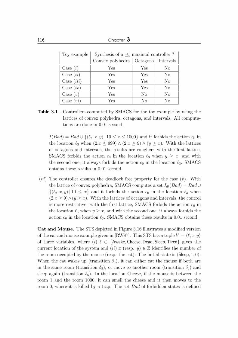
116 Chapter 3
Toy example Synthesis of a �p-maximal controller ?
Convex polyhedra Octagons Intervals
Case (i) Yes Yes No
Case (ii) Yes Yes No
Case (iii) Yes Yes No
Case (iv) Yes Yes No
Case (v) Yes No No
Case (vi) Yes No No
Table 3.1 - Controllers computed by SMACS for the toy example by using the
lattices of convex polyhedra, octagons, and intervals. All computa-
tions are done in 0.01 second.
I(Bad) = Bad ∪ {〈`2, x, y〉 | 10 ≤ x ≤ 1000} and it forbids the action c0 in
the location `3 when (2.x ≤ 999) ∧ (2.x ≥ 9) ∧ (y ≥ x). With the lattices
of octagons and intervals, the results are rougher: with the first lattice,
SMACS forbids the action c0 in the location `3 when y ≥ x, and with
the second one, it always forbids the action c0 in the location `3. SMACS
obtains these results in 0.01 second.
(vi) The controller ensures the deadlock free property for the case (v). With
the lattice of convex polyhedra, SMACS computes a set Idf (Bad) = Bad∪{〈`2, x, y〉 | 10 ≤ x} and it forbids the action c0 in the location `3 when
(2.x ≥ 9)∧(y ≥ x). With the lattices of octagons and intervals, the control
is more restrictive: with the first lattice, SMACS forbids the action c0 in
the location `3 when y ≥ x, and with the second one, it always forbids the
action c0 in the location `3. SMACS obtains these results in 0.01 second.
Cat and Mouse. The STS depicted in Figure 3.16 illustrates a modified version
of the cat and mouse example given in [RW87]. This STS has a tuple V = 〈`, x, y〉of three variables, where (i) ` ∈ {Awake,Cheese,Dead, Sleep,Tired} gives the
current location of the system and (ii) x (resp. y) ∈ Z identifies the number of
the room occupied by the mouse (resp. the cat). The initial state is 〈Sleep, 1, 0〉.When the cat wakes up (transition δ3), it can either eat the mouse if both are
in the same room (transition δ5), or move to another room (transition δ4) and
sleep again (transition δ6). In the location Cheese, if the mouse is between the
room 1 and the room 1000, it can smell the cheese and it then moves to the
room 0, where it is killed by a trap. The set Bad of forbidden states is defined

Synthesis of Centralized Memoryless Controllers with Partial Observationfor Infinite State Systems 117
δ1 = 〈runaway;TTDV ;x := x + 1〉
δ2 = 〈up2rooms;TTDV ;x := 2 ∗ x〉δ7 = 〈smellcheese;
1 ≤ x ≤ 1000;x := x− 1〉δ3 = 〈wakeup;TTDV ; IdDV 〉
δ6 = 〈sleep;TTDV ; IdDV 〉
δ5 = 〈cateat;x = y; IdDV 〉 δ8 = 〈trapped;x = 0; IdDV 〉
δ4 = 〈up2rooms;x "= y; y := 2 ∗ y〉
CheeseDeadAwake
Tired Sleep
Figure 3.16 - The cat and mouse example
dead
cheese
< x == 0 >
[trapped]{}
< x <= 1000 and x >= 1 >
[smellcheese]{x = (x - 1)}
tired
sleep
< #true >
[sleep]{y = y}
awake
< x == y >
[cateat]{}
< x != y > [up2room]
{y = (y * 2)}
< #true and not (((500 + (-1 * x)) + (0 * y)) >= 0
and ((0 + (1 * x)) + (0 * y)) >= 0) > [up2room]
{x = (x * 2)}
< #true and
not (((0 + (-1 * x)) + (1 * y)) == 0) > [wakeup]
{}
< #true > [runaway]
{x = (x + 1)}
Figure 3.17 - Controlled system generated by SMACS for the cat and mouse
example when the controller has a full observation of the system
and when the deadlock free property is not ensured.
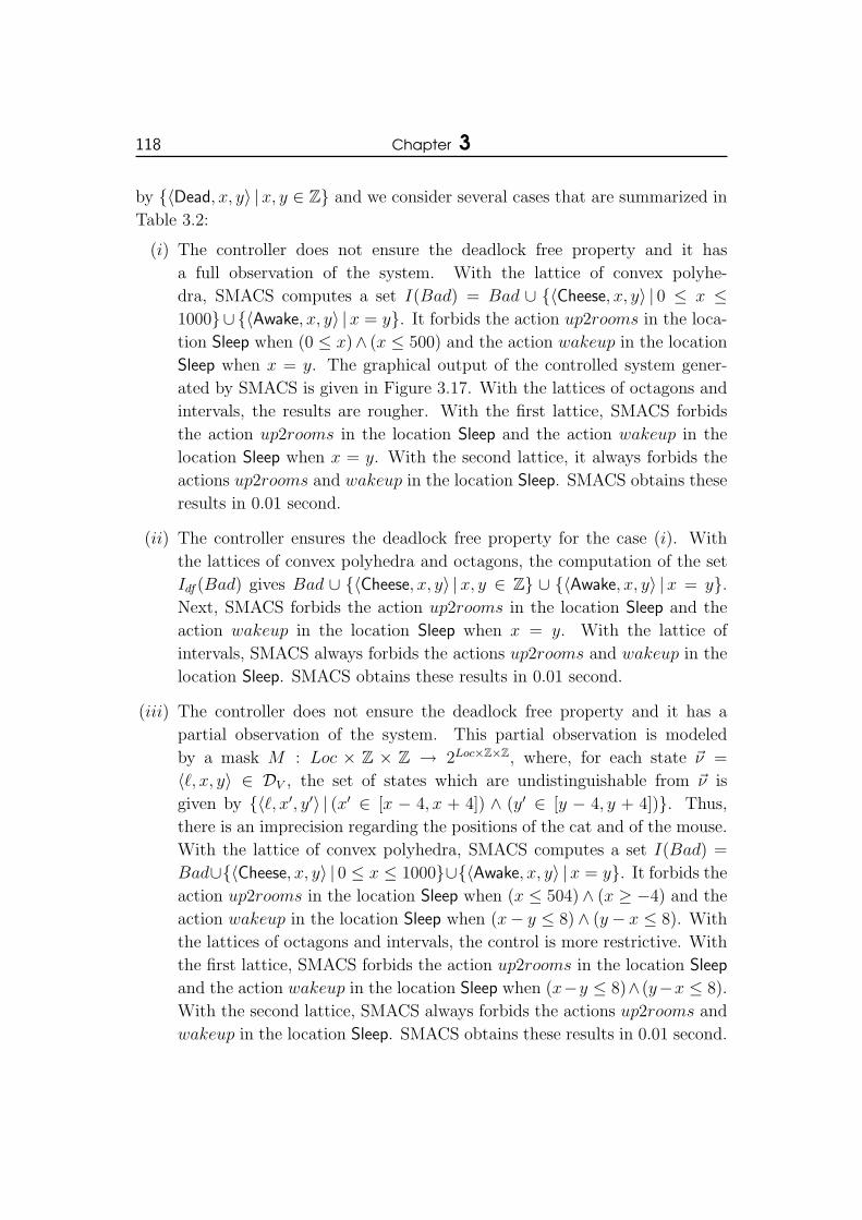
118 Chapter 3
by {〈Dead, x, y〉 |x, y ∈ Z} and we consider several cases that are summarized in
Table 3.2:
(i) The controller does not ensure the deadlock free property and it has
a full observation of the system. With the lattice of convex polyhe-
dra, SMACS computes a set I(Bad) = Bad ∪ {〈Cheese, x, y〉 | 0 ≤ x ≤1000}∪ {〈Awake, x, y〉 |x = y}. It forbids the action up2rooms in the loca-
tion Sleep when (0 ≤ x)∧ (x ≤ 500) and the action wakeup in the location
Sleep when x = y. The graphical output of the controlled system gener-
ated by SMACS is given in Figure 3.17. With the lattices of octagons and
intervals, the results are rougher. With the first lattice, SMACS forbids
the action up2rooms in the location Sleep and the action wakeup in the
location Sleep when x = y. With the second lattice, it always forbids the
actions up2rooms and wakeup in the location Sleep. SMACS obtains these
results in 0.01 second.
(ii) The controller ensures the deadlock free property for the case (i). With
the lattices of convex polyhedra and octagons, the computation of the set
Idf (Bad) gives Bad ∪ {〈Cheese, x, y〉 |x, y ∈ Z} ∪ {〈Awake, x, y〉 |x = y}.Next, SMACS forbids the action up2rooms in the location Sleep and the
action wakeup in the location Sleep when x = y. With the lattice of
intervals, SMACS always forbids the actions up2rooms and wakeup in the
location Sleep. SMACS obtains these results in 0.01 second.
(iii) The controller does not ensure the deadlock free property and it has a
partial observation of the system. This partial observation is modeled
by a mask M : Loc × Z × Z → 2Loc×Z×Z, where, for each state ~ν =
〈`, x, y〉 ∈ DV , the set of states which are undistinguishable from ~ν is
given by {〈`, x′, y′〉 | (x′ ∈ [x − 4, x + 4]) ∧ (y′ ∈ [y − 4, y + 4])}. Thus,
there is an imprecision regarding the positions of the cat and of the mouse.
With the lattice of convex polyhedra, SMACS computes a set I(Bad) =
Bad∪{〈Cheese, x, y〉 | 0 ≤ x ≤ 1000}∪{〈Awake, x, y〉 |x = y}. It forbids the
action up2rooms in the location Sleep when (x ≤ 504)∧ (x ≥ −4) and the
action wakeup in the location Sleep when (x− y ≤ 8) ∧ (y − x ≤ 8). With
the lattices of octagons and intervals, the control is more restrictive. With
the first lattice, SMACS forbids the action up2rooms in the location Sleep
and the action wakeup in the location Sleep when (x−y ≤ 8)∧(y−x ≤ 8).
With the second lattice, SMACS always forbids the actions up2rooms and
wakeup in the location Sleep. SMACS obtains these results in 0.01 second.

Synthesis of Centralized Memoryless Controllers with Partial Observationfor Infinite State Systems 119
(iv) The controller ensures the deadlock free property for the case (iii). With
the lattices of convex polyhedra and octagons, the computation of the set
Idf (Bad) gives Bad ∪ {〈Cheese, x, y〉 |x, y ∈ Z} ∪ {〈Awake, x, y〉 |x = y}.SMACS forbids the action up2rooms in the location Sleep and the action
wakeup in the location Sleep when (x − y ≤ 8) ∧ (y − x ≤ 8). With
the lattice of intervals, SMACS always forbids the actions up2rooms and
wakeup in the location Sleep. SMACS obtains these results in 0.01 second.
(v) The controller does not ensure the deadlock free property and it has a
partial observation of the system. This partial observation is modeled
by a mask M : Loc × Z × Z → 2Loc×Z×Z, where, for each state ~ν =
〈`, x, y〉 ∈ DV , the set of states which are undistinguishable from ~ν is
given by {〈`, x, y′〉 | y′ ∈ Z}. Thus, the controller does not observe the
variable y. With the lattice of convex polyhedra, SMACS computes a set
I(Bad) = Bad∪{〈Cheese, x, y〉 | 0 ≤ x ≤ 1000}∪{〈Awake, x, y〉 |x = y}. It
forbids the action up2rooms in the location Sleep when (x ≤ 500)∧(x ≥ 0)
and the action wakeup in the location Sleep (because it does not observe
the variable y). With the lattices of octagons and intervals, the control is
more restrictive: SMACS always forbids the actions up2rooms and wakeup
in the location Sleep. SMACS obtains these results in 0.01 second.
(vi) The controller ensures the deadlock free property for the case (v). With
the lattices of convex polyhedra and octagons, SMACS computes a set
Idf (Bad) = Bad ∪ {〈Cheese, x, y〉 |x, y ∈ Z} ∪ {〈Awake, x, y〉 |x = y}. It
forbids the actions up2rooms and wakeup in the location Sleep. With the
lattice of intervals, SMACS computes the same controller. It obtains these
results in 0.01 second.
Producer and Consumer. We consider a modified version of the producer
and consumer example given in Figure 3.1, where the transitions δ1, δ4, δ5 and
δ8 are respectively replaced by 〈Cons; 0 ≤ y ≤ 500;x := x − 1, y := y − 1〉,〈Stop prod; TTDV
; y := 500〉, 〈Cons′; 0 ≤ y′ ≤ 500;x′ := x′ − 1, y′ := y′ − 1〉,and 〈Stop prod′; TTDV
; y′ := 500〉, which makes the system more difficult to be
controlled. The set Bad of forbidden states is defined by {〈CX, x, x′, y, y′〉 | (x ≤10)∧(y ∈ [0, 500])}∪{〈CX′, x, x′, y, y′〉 | (x′ ≤ 10)∧(y′ ∈ [0, 500])} and we consider
several cases that are summarized in Table 3.3:
(i) The controller does not ensure the deadlock free property and it has a
full observation of the system. With the lattices of convex polyhedra and

120 Chapter 3
CXP
[ConsXp]
( (yp<=500.) AND (yp >= 0.) ) {yp = (yp - 1.),xp = (xp - 1.)}
Choice
[StopConsXp]
( #true ) {}
CX
[ConsX]
( (y<=500.) AND (y >= 0.) ) {y = (y - 1.),x = (x - 1.)}
[StopConsX]
( #true ) {}
PXP
[StopProdXp]
( ( #true ) AND NOT ((((510. + (0. * x)) + (-1. * xp)) + (0. * y)) + (0. * yp)) >=0.] )
{yp = 500.}
[ProdXp] ( #true )
{xp = (xp + 1.)}
PX
[StopProdX]
( ( #true ) AND NOT ((((510. + (-1. * x)) + (0. * xp)) + (0. * y)) + (0. * yp)) >=0.] )
{y = 500.}
[ProdX]
( #true ) {x = (x + 1.)}
[ChoiceXp] ( #true )
{}
[ChoiceX] ( #true )
{}
Figure 3.18 - Controlled system generated by SMACS for the producer and con-
sumer example (where δ1 = 〈Cons; 0 ≤ y ≤ 500;x := x − 1, y :=
y − 1〉, δ4 = 〈Stop prod; TTDV; y := 500〉, δ5 = 〈Cons′; 0 ≤ y′ ≤
500;x′ := x′ − 1, y′ := y′ − 1〉, and δ8 = 〈Stop prod′; TTDV; y′ :=
500〉) when the controller has a full observation of the system and
when the deadlock free property is not ensured.

Synthesis of Centralized Memoryless Controllers with Partial Observationfor Infinite State Systems 121
Cat and mouse example Synthesis of a �p-maximal controller ?
Convex polyhedra Octagons Intervals
Case (i) Yes No No
Case (ii) Yes Yes No
Case (iii) Yes No No
Case (iv) Yes Yes No
Case (v) Yes No No
Case (vi) Yes Yes Yes
Table 3.2 - Controllers computed by SMACS for the cat and mouse example by
using the lattices of convex polyhedra, octagons, and intervals. All
computations are done in 0.01 second.
octagons, SMACS forbids the action Stop prod in the location PX when
x ≤ 510 and the action Stop prod′ in the location PX′ when x′ ≤ 510. The
graphical output of the controlled system generated by SMACS is given in
Figure 3.18. With the lattices of intervals, the control is more restrictive:
SMACS always forbids the action Stop prod in the location PX and the
action Stop prod′ in the location PX′. SMACS obtains these results in 0.01
second.
(ii) The controller does not ensure the deadlock free property and it has a par-
tial observation of the system. This partial observation is modeled by the
mask M defined in Example 3.3 i.e., for each state ~ν = 〈`, x, x′, y, y′〉 ∈DV , the set of states which are undistinguishable from ~ν, is given by
{〈`, x1, x′, y, y′〉 |x1 ∈ [x − 1, x + 1]}. With the lattices of convex poly-
hedra and octagons, SMACS forbids the action Stop prod in the location
PX when x ≤ 511 and the action Stop prod′ in the location PX′ when
x′ ≤ 510. With the lattice of intervals, SMACS always forbids the action
Stop prod in the location PX and the action Stop prod′ in the location PX′.
SMACS obtains these results in 0.01 second.
(iii) The controller does not ensure the deadlock free property and it has a
partial observation of the system. This partial observation is modeled by
a mask M where, for each state ~ν = 〈`, x, x′, y, y′〉 ∈ DV , the set of states
which are undistinguishable from ~ν, is given by {〈`, x, x′1, y, y′1〉 |x′1, y′1 ∈Z}. Thus, the controller does not observe the variables x′ and y′. With
the lattices of convex polyhedra and octagons, SMACS forbids the action
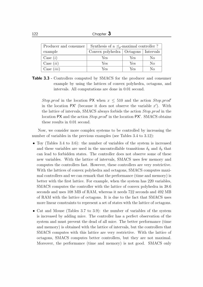
122 Chapter 3
Producer and consumer Synthesis of a �p-maximal controller ?
example Convex polyhedra Octagons Intervals
Case (i) Yes Yes No
Case (ii) Yes Yes No
Case (iii) Yes Yes No
Table 3.3 - Controllers computed by SMACS for the producer and consumer
example by using the lattices of convex polyhedra, octagons, and
intervals. All computations are done in 0.01 second.
Stop prod in the location PX when x ≤ 510 and the action Stop prod′
in the location PX′ (because it does not observe the variable x′). With
the lattice of intervals, SMACS always forbids the action Stop prod in the
location PX and the action Stop prod′ in the location PX′. SMACS obtains
these results in 0.01 second.
Now, we consider more complex systems to be controlled by increasing the
number of variables in the previous examples (see Tables 3.4 to 3.12):
• Toy (Tables 3.4 to 3.6): the number of variables of the system is increased
and these variables are used in the uncontrollable transitions δ8 and δ9 that
can lead to forbidden states. The controller does not observe some of these
new variables. With the lattice of intervals, SMACS uses few memory and
computes the controllers fast. However, these controllers are very restrictive.
With the lattices of convex polyhedra and octagons, SMACS computes maxi-
mal controllers and we can remark that the performance (time and memory) is
better with the first lattice. For example, when the system has 220 variables,
SMACS computes the controller with the lattice of convex polyhedra in 38.6
seconds and uses 108 MB of RAM, whereas it needs 722 seconds and 492 MB
of RAM with the lattice of octagons. It is due to the fact that SMACS uses
more linear constraints to represent a set of states with the lattice of octagons.
• Cat and Mouse (Tables 3.7 to 3.9): the number of variables of the system
is increased by adding mice. The controller has a perfect observation of the
system and must prevent the dead of all mice. The better performance (time
and memory) is obtained with the lattice of intervals, but the controllers that
SMACS computes with this lattice are very restrictive. With the lattice of
octagons, SMACS computes better controllers, but they are not maximal.
Moreover, the performance (time and memory) is not good. SMACS only

Synthesis of Centralized Memoryless Controllers with Partial Observationfor Infinite State Systems 123
Number of Convex polyhedra
variables in the Time Maximal �p-Maximal
toy example Memory (MB) Controller ?
30 0.28 < 12 Yes
80 2.47 60 Yes
130 8.9 72 Yes
180 21.8 96 Yes
220 38.6 108 Yes
Table 3.4 - The time (in seconds) and the memory (in MB) that SMACS uses
with the lattice of convex polyhedra to synthesize a controller for a
modified version of the toy example.
computes maximal controllers with the lattice of convex polyhedra and the
performance obtained with this lattice is better than the one obtained with
the lattice of octagons.
• Producer and Consumer (Tables 3.10 to 3.12): the system is made more com-
plex by producing n (where n > 0) kinds of parts. The production of each
kind of parts requires the definition of two variables. The control requirements
consist in ensuring that there are at least 11 parts of each kind. Moreover,
the controller does not observe the value of some variables when it belongs
to a given interval. Again, the better performance (time and memory) is ob-
tained with the lattice of intervals, but the controllers that SMACS computes
with this lattice are very rough. With the lattices of convex polyhedra and
octagons, SMACS computes maximal controllers and we can remark that the
performance (time and memory) is better with the first lattice. For example,
when the system has 160 variables, SMACS computes the controller with the
lattice of convex polyhedra in 92.3 seconds and uses 624 MB of RAM, whereas
it needs 1181 seconds and 2124 MB of RAM with the lattice of octagons.

124 Chapter 3
Number of Octagons
variables in the Time Maximal �p-Maximal
toy example Memory (MB) Controller ?
30 2.4 24 Yes
80 36.9 240 Yes
130 157.7 312 Yes
180 391.1 396 Yes
220 722 492 Yes
Table 3.5 - The time (in seconds) and the memory (in MB) that SMACS uses
with the lattice of octagons to synthesize a controller for a modified
version of the toy example.
Number of Intervals
variables in the Time Maximal �p-Maximal
toy example Memory (MB) Controller ?
30 0.06 < 12 No
80 0.08 < 12 No
130 0.15 < 12 No
180 0.25 < 12 No
220 0.37 < 12 No
Table 3.6 - The time (in seconds) and the memory (in MB) that SMACS uses
with the lattice of intervals to synthesize a controller for a modified
version of the toy example.
Number of variables Convex polyhedra
in the cat and Time Maximal �p-Maximal
mouse example Memory (MB) Controller ?
10 0.08 < 12 Yes
40 0.8 36 Yes
90 4.3 60 Yes
140 14.3 84 Yes
200 36.1 108 Yes
Table 3.7 - The time (in seconds) and the memory (in MB) that SMACS uses
with the lattice of convex polyhedra to synthesize a controller for a
modified version of the cat and mouse example.

Synthesis of Centralized Memoryless Controllers with Partial Observationfor Infinite State Systems 125
Number of variables Octagons
in the cat and mouse Time Maximal �p-Maximal
example Memory (MB) Controller ?
10 0.3 < 12 No
40 5.8 216 No
90 58.6 228 No
140 210.3 372 No
200 601 468 No
Table 3.8 - The time (in seconds) and the memory (in MB) that SMACS uses
with the lattice of octagons to synthesize a controller for a modified
version of the cat and mouse example.
Number of variables Intervals
in the cat and mouse Time Maximal �p-Maximal
example Memory (MB) Controller ?
10 0.03 < 12 No
40 0.06 < 12 No
90 0.15 < 12 No
140 0.22 < 12 No
200 0.41 < 12 No
Table 3.9 - The time (in seconds) and the memory (in MB) that SMACS uses
with the lattice of intervals to synthesize a controller for a modified
version of the cat and mouse example.
Number of variables Convex polyhedra
in the producer and Time Maximal �p-Maximal
consumer example Memory (MB) Controller ?
40 1.26 96 Yes
80 8.8 168 Yes
120 33.4 288 Yes
160 92.3 624 Yes
180 141.2 852 Yes
Table 3.10 - The time (in seconds) and the memory (in MB) that SMACS uses
with the lattice of convex polyhedra to synthesize a controller for
a modified version of the producer and consumer example.
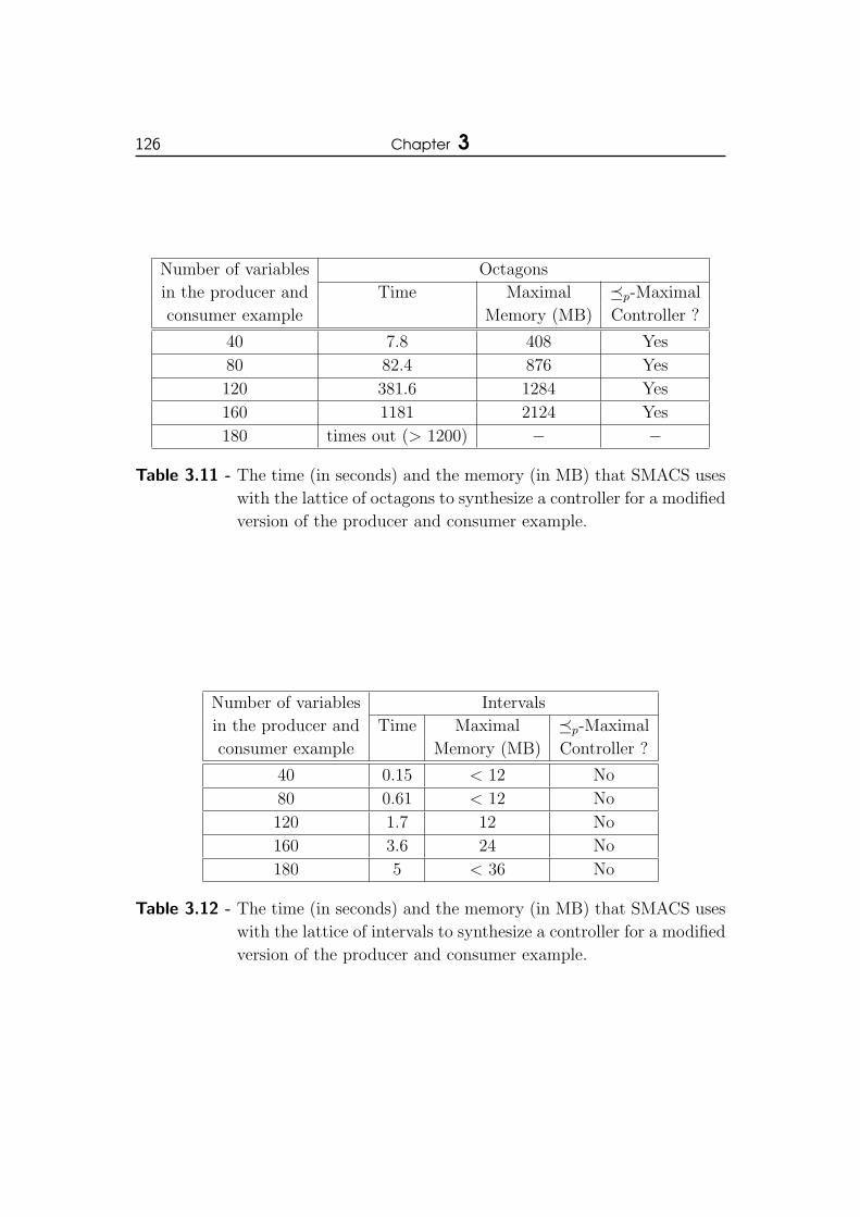
126 Chapter 3
Number of variables Octagons
in the producer and Time Maximal �p-Maximal
consumer example Memory (MB) Controller ?
40 7.8 408 Yes
80 82.4 876 Yes
120 381.6 1284 Yes
160 1181 2124 Yes
180 times out (> 1200) − −
Table 3.11 - The time (in seconds) and the memory (in MB) that SMACS uses
with the lattice of octagons to synthesize a controller for a modified
version of the producer and consumer example.
Number of variables Intervals
in the producer and Time Maximal �p-Maximal
consumer example Memory (MB) Controller ?
40 0.15 < 12 No
80 0.61 < 12 No
120 1.7 12 No
160 3.6 24 No
180 5 < 36 No
Table 3.12 - The time (in seconds) and the memory (in MB) that SMACS uses
with the lattice of intervals to synthesize a controller for a modified
version of the producer and consumer example.
Chapter
4Synthesis of Centralized k-memory
and Online Controllers with Partial
Observation for Infinite State Sys-
tems
In the previous chapter, we provided methods to synthesize memoryless
controllers for infinite state systems under partial observation. In these
algorithms, the control decisions taken by the controller are only based
on the current observation that it receives from the system. A way to improve
the permissiveness of the controllers is to provide them with memory in order to
retain the history of the execution of the system partially or totally; this actually
allows the controller to have a finer knowledge of the set of states in which the
system can be. There are mainly two ways to use this memory:
• The first possibility is to record the last k (where k is a finite number) ob-
servations received from the system. So, the controller knows a part of the
history of the execution of the system. It can then use this information to
refine its knowledge of the possible paths taken by the system and hence to
have more accurate control decisions. These controllers are called k-memory
controllers.
• The second possibility is to retain the set of states in which the system can

128 Chapter 4
be. More precisely, during the execution of the system, when the controller
receives an observation from the system, it updates its estimate of the current
state of the system from this observation and its control decisions. Next,
it uses this estimate to determine the actions that it forbids. That allows,
in some sense, to retain the entire history of the execution of the system,
because the estimate computed by the controller is based on all observations
received from the beginning of the execution of the system and on all its
control decisions. These controllers are called online controllers.
In this chapter, we study these two possibilities. First, in section 4.1, we de-
fine an algorithm which synthesizes a k-memory controller for the state avoidance
control problem. Next, in section 4.2, we define an algorithm that synthesizes
an online controller. In section 4.3, we compare the permissiveness of the mem-
oryless, k-memory and online controllers synthesized by our algorithms.
4.1 Synthesis of k-Memory Controllers
In this section, we extend the method presented in chapter 3 to synthesize
k-memory controllers for the state avoidance control problem. First, in sec-
tion 4.1.1, we define the framework that we use. Next, in section 4.1.2, we define
a semi-algorithm which computes a k-memory controller for the state avoidance
control problem. Finally, in section 4.1.3, we explain how to extend this semi-
algorithm by using abstract interpretation to obtain an effective algorithm.
4.1.1 Framework and State Avoidance Control Problem
The framework is quite similar to the one defined in section 3.3; the only changes
concern the definition of the controller and hence the definition of the controlled
system. In this framework, a k-memory controller can retain the last k obser-
vations that it received from the system and use this information to choose the
actions to be forbidden. It is formally defined as follows:
Definition 4.1 (k-Memory Controller)
Given an STS T = 〈V,Θ0,Σ,∆〉, an observer 〈Obs,M〉, and an integer1k ≥ 1,
a k-memory controller with partial observation for the system T is a pair
Ck = 〈Sk, Ek〉, where:

Synthesis of Centralized k-memory and Online Controllers with PartialObservation for Infinite State Systems 129
• Sk : (DObs)k → 2Σc is a supervisory function which defines,
for each k-tuple of observations 〈obs1, . . . , obsk〉 ∈ (DObs)k, a set
Sk(〈obs1, . . . , obsk〉) of controllable actions that have to be forbidden
when obs1, . . . , obsk are the last k observations received by the controller
from the system (note that obsk is the last observation received from the
system).
• Ek ⊆ DV is a set of states, which restricts the set of initial states of T .
Let 〈obs1, . . . , obsk〉 be the content of the controller’s memory (where obsk cor-
responds to the last observation that the controller received from the system),
when the controller receives a new observation obsk+1, its memory evolves from
〈obs1, . . . , obsk〉 to 〈obs2, . . . , obsk+1〉. Note that at the beginning of the execution
of the system (before the first observation), the memory of the controller is ini-
tialized to 〈Γ, . . . ,Γ〉 (Γ is thus a special symbol which means that a component
of the memory contains no observation).
The controlled system T/Ckresulting from the interaction between the system
T and the k-memory controller Ck is defined by an STS with k additional vari-
ables, which provide the last k observations that the controller received from the
system. It is formally defined as follows:
Definition 4.2 (Controlled System)
Given an STS T = 〈V,Θ0,Σ,∆〉, an observer 〈Obs,M〉, and a k-memory
controller Ck = 〈Sk, Ek〉, the system T controlled by Ck, denoted by T/Ck, is an
STS including observations which is defined by T/Ck
def= 〈V/Ck
, (Θ0)/Ck,Σ,∆/Ck
〉,where:
• V/Ck
def= V ·∪ 〈Obs1, . . . , Obsk〉 is a pair composed of the tuple of variables
V and of the k-tuple of variables 〈Obs1, . . . , Obsk〉. The domain DObsi
of each variable Obsi (∀i ∈ [1, k]) is defined by DObsi
def= DObs ∪ {Γ}.
• (Θ0)/Ck
def= {〈~ν, 〈Γ, . . . ,Γ, obs〉〉 | (~ν ∈ (Θ0 \ Ek)) ∧ (obs ∈ M(~ν))} is the
set of initial states.
1Note that k 6=∞.
130 Chapter 4
• ∆/Ckis defined from ∆ as follows: for each transition 〈σ,G,A〉 ∈
∆, we define a new transition 〈σ,G/Ck, A/Ck
〉def∈ ∆/Ck
, where
(i) G/Ck
def= {〈~ν, 〈obs1, . . . , obsk〉〉 | (~ν ∈ G) ∧ (obsk ∈ M(~ν)) ∧
(σ 6∈ Sk(〈obs1, . . . , obsk〉))}, and (ii) A/Ckis defined, for each
~ν1 ∈ DV and for each 〈obs1, . . . , obsk〉 ∈ (DObs)k−1 × M(~ν1),
by A/Ck(〈~ν1, 〈obs1, . . . , obsk〉〉)
def= {〈~ν2, 〈obs2, . . . , obsk, obsk+1〉〉 | (~ν2 =
A(~ν1)) ∧ (obsk+1 ∈M(~ν2))}.
This definition generalizes Definition 3.10. A state 〈~ν, 〈obs1, . . . , obsk〉〉 (with
obsk ∈M(~ν)) of the controlled system models the fact that when the system was
in the state ~ν, the observations obs1, . . . , obsk were the last k information that
the controller received from the system. The guards and the update functions of
the controlled system T/Ckare computed from the ones of the system T by taking
into account the control decisions of the controller Ck and the observations that
it can receive from the system.
• Guards: A transition 〈σ,G/Ck, A/Ck
〉 ∈ ∆/Ck, defined from the transition
δ = 〈σ,G,A〉 ∈ ∆, can be fired from a state 〈~ν, 〈obs1, . . . , obsk〉〉 ∈ DV/Ckin
the controlled system if and only if (i) δ can be fired from ~ν in T , (ii) ~ν
is compatible with obsk, and (iii) σ is not forbidden by the controller Ck in
〈obs1, . . . , obsk〉.
• Update functions: The update function A/Ckof the transition
〈σ,G/Ck, A/Ck
〉 ∈ ∆/Ck, defined from the transition δ = 〈σ,G,A〉 ∈ ∆, al-
lows the controlled system to reach the state 〈~ν2, 〈obs2, . . . , obsk, obsk+1〉〉 ∈DV/Ck
from a state 〈~ν1, 〈obs1, . . . , obsk〉〉 ∈ DV/Ckif and only if (i) the
update function A allows the system T to reach ~ν2 from ~ν1, and (ii)
~ν2 is compatible with obsk+1. The definition of A/Ckis based on the
evolution of the controller’s memory when it receives a new observation
obsk+1: the memory evolves from 〈obs1, . . . , obsk〉 to 〈obs2, . . . , obsk, obsk+1〉.Moreover, the update functions A/Ck
satisfy the following property:
(〈~ν2, 〈obs2, . . . , obsk, obsk+1〉〉 ∈ A/Ck(〈~ν1, 〈obs1, . . . , obsk〉〉)) ⇒ (∀obs′k+1 ∈
M(~ν2) : 〈~ν2, 〈obs2, . . . , obsk, obs′k+1〉〉 ∈ A/Ck
(〈~ν1, 〈obs1, . . . , obsk〉〉)). This
property means that when the system arrives in a state ~ν2, the controller
can receive any observation of ~ν2.

Synthesis of Centralized k-memory and Online Controllers with PartialObservation for Infinite State Systems 131
The problem, that we want to solve, is the basic problem adapted to this
framework2. It is formally defined as follows:
Problem 4.1 (Memory Basic State Avoidance Control Problem)
Given an STS T = 〈V,Θ0,Σ,∆〉, an observer 〈Obs,M〉 and a predicate Bad,
which represents a set of forbidden states, the memory basic state avoidance
control problem (memory basic problem for short) consists in computing a k-
memory controller Ck = 〈Sk, Ek〉 such that (i) ReachableT/Ck∆/Ck
((Θ0)/Ck) 6= ∅ and
(ii)(Reachable
T/Ck∆/Ck
((Θ0)/Ck)⌋
[1]
)∩Bad = ∅.
As a reminder,(Reachable
T/Ck∆/Ck
((Θ0)/Ck)⌋
[1]
)= {~ν | ∃〈~ν, 〈obs1, . . . , obsk〉〉 ∈
ReachableT/Ck∆/Ck
((Θ0)/Ck)} (see section 1.1). This problem consists in synthesizing
a non-trivial and valid k-memory controller.
Note that the memoryless controller is a particular case of the k-memory con-
troller, since it corresponds to the case where k = 1. Therefore, all propositions
proved in section 3.3.4 remain valid. In particular, the memory basic problem is
undecidable, which explains the use of abstract interpretation in section 4.1.3 to
obtain an effective algorithm.
4.1.2 Semi-algorithm for the Memory Basic Problem
Our algorithm, which synthesizes controllers for the memory basic problem, is
an extension of the one defined for the memoryless case and is also composed of
two parts.
Computation of I(Bad). The set I(Bad) of states leading uncontrollably to
Bad is given by the fixpoint equation defined in (3.1) which, as a reminder, is
equal to lfp⊆(λB.Bad ∪ PreT∆uc(B)).
Computation of the Controller Ck. The second step consists in computing
the controller Ck whose aim is to forbid all controllable actions that can lead to
a state in I(Bad). For that, we first define the function Fk : Σ× 2DV → 2(DObs)k,
which gives, for each action σ ∈ Σ and set B ⊆ DV of states to be forbidden,
the set Fk(σ,B) of sequences of observations of length less than or equal to k for
2We only consider this case to remain quite concise, but controllers ensuring the deadlockfree property can also be computed for this framework.

132 Chapter 4
which the action σ must be forbidden. Each k-tuple 〈obs1, . . . , obsk〉 ∈ Fk(σ,B)
should correspond to a possible sequence of observations of the system. Moreover,
the last observation obsk of this sequence must be such that there exists a state
~ν compatible with this observation which leads to B by a transition labeled by
σ.
To obtain Fk(σ,B), we compute all possible sequences of states of length k
that end by a state ~ν leading to B by a transition labeled by σ and all possible
sequences of states of length strictly less than k that start by an initial state
and that ends by a state ~ν leading to B by a transition labeled by σ. Moreover,
we apply the mask M to these sequences to take into account the paths that are
undistinguishable from them. We compute this set with the following algorithm:
Algorithm 4. In order to compute Fk(σ,B), Algorithm 4 considers all sequences
δ1, . . . , δk of transitions of length k (with δk labeled by σ) and, for each of these
sequences, it iteratively computes (line 10) the sequences of observations that
can occur by executing this sequence. It starts this iteration by computing the
set Pred of states that do not belong to B and that lead to B by δk (line 11), and
by applying the mask M to this set (line 25). Next, for each δi (∀i ∈ [1, k − 1]),
it performs a similar operation by computing the set of states that are not in B
and that lead to the set Pred (computed at the previous iteration) by δi (line 11)
and by applying the mask M to this set (line 25). However, two particular cases
must be considered:
• some sequences δ1, . . . , δk of transitions of length k cannot lead to B. This
situation is detected when the set Pred computed for a transition δi is empty
(line 13). In this case, the computations for this sequence are stopped.
• some sequences of transitions of length strictly less than k can lead toB. These
sequences start from an initial state and this situation is thus detected when
the set Pred computed for a transition δi contains initial states (line 17).
These sequences of transitions generate sequences of observations of length
strictly less than k and we add some symbols Γ to the beginning of them to
obtain sequences of observations of length k that we add to the set Fk(σ,B).
Adding these symbols Γ does not make erroneous the computation of the con-
troller, because, at the beginning of the execution of the system, the memory
of the controller is initialized to 〈Γ, . . . ,Γ〉.
The output Fk(σ,B) of Algorithm 4 corresponds to a finite union of k-tuples
K of sets of observations. This function forbids the action σ after a sequence
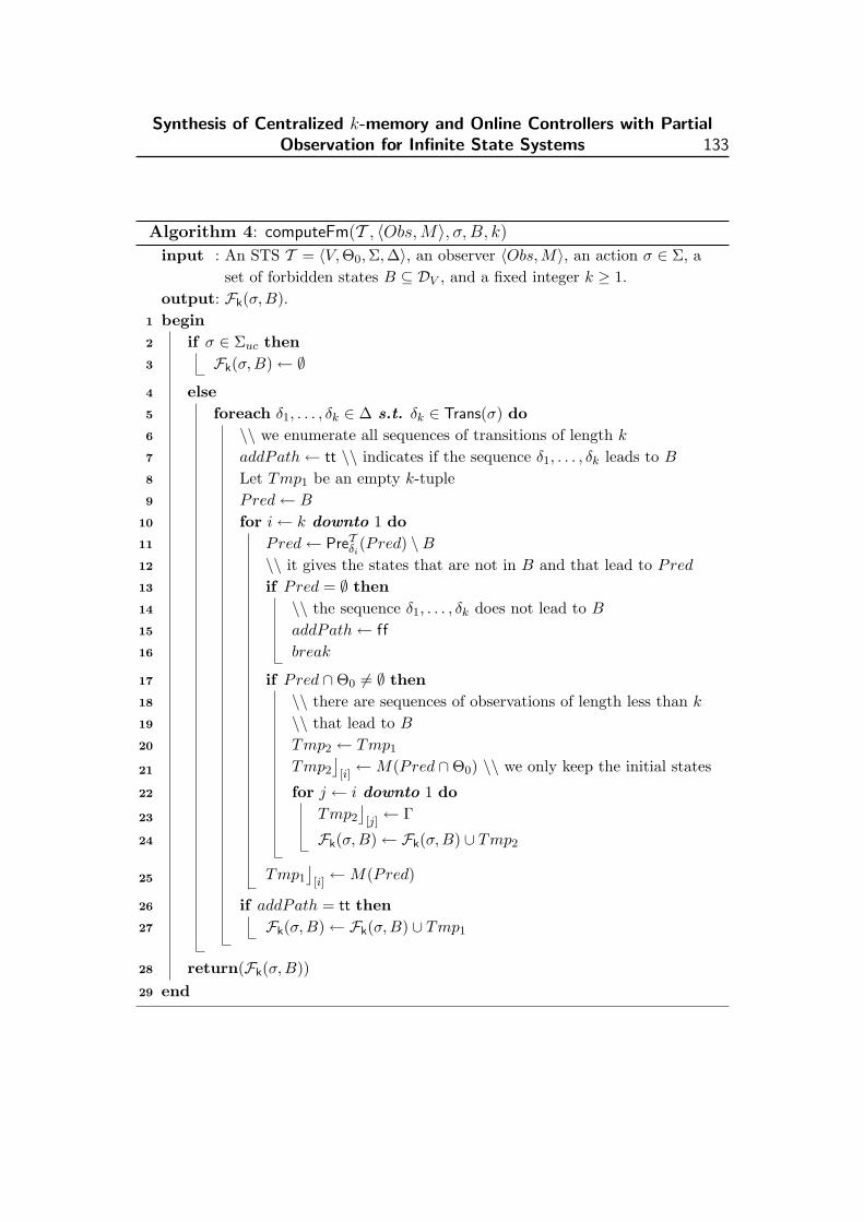
Synthesis of Centralized k-memory and Online Controllers with PartialObservation for Infinite State Systems 133
Algorithm 4: computeFm(T , 〈Obs,M〉, σ, B, k)input : An STS T = 〈V,Θ0,Σ,∆〉, an observer 〈Obs, M〉, an action σ ∈ Σ, a
set of forbidden states B ⊆ DV , and a fixed integer k ≥ 1.output: Fk(σ,B).begin1
if σ ∈ Σuc then2
Fk(σ,B)← ∅3
else4
foreach δ1, . . . , δk ∈ ∆ s.t. δk ∈ Trans(σ) do5
\\ we enumerate all sequences of transitions of length k6
addPath← tt \\ indicates if the sequence δ1, . . . , δk leads to B7
Let Tmp1 be an empty k-tuple8
Pred← B9
for i← k downto 1 do10
Pred← PreTδi(Pred) \B11
\\ it gives the states that are not in B and that lead to Pred12
if Pred = ∅ then13
\\ the sequence δ1, . . . , δk does not lead to B14
addPath← ff15
break16
if Pred ∩Θ0 6= ∅ then17
\\ there are sequences of observations of length less than k18
\\ that lead to B19
Tmp2 ← Tmp120
Tmp2
⌋[i]←M(Pred ∩Θ0) \\ we only keep the initial states21
for j ← i downto 1 do22
Tmp2
⌋[j]← Γ23
Fk(σ,B)← Fk(σ,B) ∪ Tmp224
Tmp1
⌋[i]←M(Pred)25
if addPath = tt then26
Fk(σ,B)← Fk(σ,B) ∪ Tmp127
return(Fk(σ,B))28
end29

134 Chapter 4
δ3 = 〈σ3;TTDV ;x := x/2〉
δ1 = 〈σ1;TTDV ;x := x + 1〉 δ2 = 〈σ2;TTDV ;x := x + 1〉
!0 !2
!1
Figure 4.1 - Computation of the function Fk.
〈obs1, . . . , obsk〉 of observations if and only if 〈obs1, . . . , obsk〉 belongs to one of
these k-tuples K.
Example 4.1
The STS depicted in Figure 4.1 illustrates Algorithm 4. This system has a
tuple V = 〈`, x〉 of two variables, where (i) ` ∈ {`0, `1, `2}, and (ii) x ∈ N0.
The set Θ0 of initial states is defined by {〈`0, 5〉, 〈`0, 6〉, 〈`0, 8〉, 〈`0, 10〉} and the
set B = {〈`2, 10〉, 〈`2, 12〉}. The controller perfectly observes the system. The
computation of Fk(σ3, B) for a 2-memory controller gives 〈Γ, {〈`0, 5〉, 〈`0, 6〉}〉and the computation of Fk(σ2, B) gives 〈{〈`0, 8〉, 〈`0, 10〉}, {〈`1, 9〉, 〈`1, 11〉}〉.For example, Fk forbids σ2 after the sequence of observations 〈〈`0, 10〉, 〈`1, 11〉〉.
One can note that our computation of the function Fk is only an overapproxi-
mation of the sequences of observations leading to B. Indeed, in Example 4.1,
the sequence of observations 〈〈`0, 8〉, 〈`1, 11〉〉 belongs to Fk(σ2, B), whereas it
cannot occur in the system. An exact computation should record all possible
and precise paths leading to B, but with infinite state spaces, we cannot always
represent all these paths in a finite way (they are potentially infinite).
Next, by using this function Fk, we can define the controller Ck in the following
way:
Ckdef= 〈Sk, Ek〉 (4.1)
with the elements Sk and Ek defined as follows:
• the supervisory function Sk is given, for each k-tuple 〈obs1, . . . , obsk〉 corre-
sponding to a possible content of the memory of the controller, by:
Sk(〈obs1, . . . , obsk〉)def= {σ ∈ Σc | 〈obs1, . . . , obsk〉 ∈ Fk(σ, I(Bad))} (4.2)

Synthesis of Centralized k-memory and Online Controllers with PartialObservation for Infinite State Systems 135
It means that σ is forbidden after the sequence of observations 〈obs1, . . . , obsk〉if I(Bad) is reachable by a transition labeled by σ after this sequence.
• the set Ekdef= I(Bad). It prevents the controlled system from beginning its
execution in a state which can lead to Bad by a sequence of uncontrollable
transitions.
The set I(Bad) and the function Fk are computed offline. Next, during
the execution of the system, when the controller receives a new observation, it
updates the content of its memory and computes online the function Sk from
this content to obtain the actions to be forbidden.
Example 4.2
In this example, we illustrate the computation of the k-memory controller and
we show that it provides a better control than the memoryless controller.
We consider the system defined in Example 3.5 where, as a reminder, (i)
Bad = {〈CX, x, x′, y, y′〉 | (x ≤ 1000) ∧ (y ∈ [0, 2])}, (ii) I(Bad) = Bad ∪{〈CX, x, x′, y, y′〉 | [(x ≤ 1001)∧ (y ∈ [1, 2])]∨ [(x ≤ 1002)∧ (y = 2)]}, and (iii)
the controller cannot distinguish a state 〈`, x, x′, y, y′〉 ∈ DV from the states in
the set {〈`, x1, x′, y, y′〉 |x1 ∈ [x− 1, x+ 1]}.
The computation of the function Fk for a 2-memory controller gives the follow-
ing values: (i) Fk(Stop prod, I(Bad)) = 〈M({〈`, x, x′, y, y′〉 | [(` = PX) ∧ (x ≤1001)] ∨ [(` = Choice) ∧ (x ≤ 1002)]}),M({〈PX, x, x′, y, y′〉 |x ≤ 1002})〉, and
(ii) Fk(σ, I(Bad)) = ∅ for each σ ∈ Σ \ {Stop prod}.Therefore, the supervisory function Sk forbids the action Stop prod if the cur-
rent state of the system belongs to the set {〈PX, x, x′, y, y′〉 |x ≤ 1003} and
if the previous state of the system belongs to the set {〈`, x, x′, y, y′〉 | [(` =
PX) ∧ (x ≤ 1002)] ∨ [(` = Choice) ∧ (x ≤ 1003)]}.This 2-memory controller is strictly more permissive than the memoryless con-
troller C computed in Example 3.5, which always forbids the action Stop prod
when the current state of the system belongs to the set {〈PX, x, x′, y, y′〉 |x ≤1003}. In Proposition 4.4, we prove that a k-memory controller is always more
permissive than a memoryless controller.
The following property proves that our algorithm synthesizes correct con-
trollers for the memory basic problem:

136 Chapter 4
Proposition 4.1
Given an STS T = 〈V,Θ0,Σ,∆〉, an observer 〈Obs,M〉 and a predicate Bad,
which represents a set of forbidden states, the controller Ck = 〈Sk, Ek〉, defined
in (4.1), solves the memory basic problem (when Θ0 6⊆ Ek).
Proof
We prove by induction on the length n of the sequences of transitions
(these sequences begin in an initial state) that(Reachable
T/Ck∆/Ck
((Θ0)/Ck)⌋
[1]
)∩
I(Bad) = ∅. Since Bad ⊆ I(Bad), this property implies that(Reachable
T/Ck∆/Ck
((Θ0)/Ck)⌋
[1]
)∩Bad = ∅.
• Base case (n = 0): the execution of the controlled system T/Ckstarts in
a state which does not belong to I(Bad), since (Θ0)/Ck
⌋[1]
= Θ0 \ Ek =
Θ0 \ I(Bad).
• Induction step: we suppose that the proposition holds for the sequences
of transitions of length less than or equal to n and we prove that this
property remains true for the sequences of transitions of length n+1. By
induction hypothesis, each state ~ν1 reachable by a sequence of transitions
of length n does not belong to I(Bad) and we show that each transition
δ = 〈σ,G,A〉 ∈ ∆, which can lead to a state ~ν2 ∈ I(Bad) from this state
~ν1 in the system T , cannot be fired from ~ν1 in the controlled system T/Ck.
For that, we consider two cases :
• if δ ∈ ∆c, then M(~ν1) ⊆ M(PreTδ (I(Bad)) \ I(Bad)), because
~ν1 ∈ (PreTδ (I(Bad)) \ I(Bad)). This transition cannot be fired from
~ν1 in the controlled system T/Ck, because by definition of Fk (see Algo-
rithm 4) and by definition of Sk (see (4.2)), σ is forbidden after each
k-tuple 〈obs1, . . . , obsk〉 which ends by an observation obsk ∈ M(~ν1)
and which corresponds to a possible execution of T/Ck.
• if δ ∈ ∆uc, then ~ν2 ∈ I(Bad) (by (3.1)), which is impossible by
hypothesis.
Hence, in the controlled system, the forbidden state ~ν2 cannot be reached
from the state ~ν1 by the transition δ.

Synthesis of Centralized k-memory and Online Controllers with PartialObservation for Infinite State Systems 137
4.1.3 Effective Algorithm for the Memory Basic Problem
As in chapter 3, an effective algorithm can be obtained by using abstract in-
terpretation techniques. More precisely, we first compute an overapproximation
I ′(Bad) of I(Bad) (see section 3.4.2 for the details). Next, we transpose the func-
tion Fk (more precisely, we transpose Algorithm 4) into the abstract lattice and
we obtain the abstract function F ]k (the computation of this function may thus
require overapproximations). Finally, we define our controller Ck = 〈Sk, I′(Bad)〉
as in (4.1) by using I ′(Bad) and F ]k instead of I(Bad) and Fk.
4.2 Synthesis of Online Controllers
In this section, we present a method which synthesizes an online controller for the
state avoidance control problem. First, in section 4.2.1, we define the framework
that we use. Next, in section 4.2.2, we define a semi-algorithm which computes an
online controller for the state avoidance control problem. Finally, in section 4.2.3,
we explain how to extend this semi-algorithm by using abstract interpretation
to obtain an effective algorithm.
4.2.1 Framework and State Avoidance Control Problem
The framework is quite similar to the one defined in section 3.3; the only changes
concern the definition of the controller and hence the definition of the controlled
system. In this framework, an online controller can compute (and retain) an
estimate of the current state of the system and use this information to choose
the actions to be forbidden. It is formally defined as follows:
Definition 4.3 (Online Controller)
Given an STS T = 〈V,Θ0,Σ,∆〉, and an observer 〈Obs,M〉, an online con-
troller with partial observation for the system T is a pair Co = 〈So, Eo〉, where:
• So : 2DV → 2Σc is a supervisory function which defines, for each subset
Pi ⊆ DV , a set So(Pi) of controllable actions that have to be forbidden
when Pi is the estimate of the current state of the system computed by
the controller.
• Eo ⊆ DV is a set of states, which restricts the set of initial states of T .

138 Chapter 4
The estimation Pi of the possible current states of the system is reevaluated by
the controller at each step of the execution of the system and its computation is
detailed in section 4.2.2.
A system T under the control of a controller Co cannot be characterized by a
single STS as in the memoryless and k-memory cases. Indeed, the controller Cocomputes the forbidden actions from the state estimate Pi, whose value changes
during the execution of T ; thus this computation depends on the history of the
execution of T . We have then decided to formalize the behavior of the system
T under the control of Co by using the concept of controlled executions which
characterizes the executions that can occur in this system:
Definition 4.4 (Controlled Execution)
Given an STS T = 〈V,Θ0,Σ,∆〉, an observer 〈Obs,M〉, an online controller
Co = 〈So, Eo〉, and an execution s = ~ν1〈σ2,G2,A2〉−−−−−−→ ~ν2
〈σ3,G3,A3〉−−−−−−→ . . .〈σn,Gn,An〉−−−−−−→ ~νn
of T , s is a controlled execution of the system T under the control of Co if it
satisfies the following conditions:
• ~ν1 ∈ Θ0 \ Eo
• when the system arrives in the state ~νi (∀i ∈ [1, n − 1]), the controller
Co computes a state estimate Pi such that σi+1 6∈ So(Pi).
A controlled execution is thus an execution that can occur in the system T under
the control of Co.The problem, that we want to solve, is the basic problem adapted to this
framework3. It is formally defined as follows:
Problem 4.2 (Online Basic State Avoidance Control Problem)
Given an STS T = 〈V,Θ0,Σ,∆〉, an observer 〈Obs,M〉 and a predicate Bad,
which represents a set of forbidden states, the online basic state avoidance
control problem (online basic problem for short) consists in computing an online
controller Co = 〈So, Eo〉 such that (i) Θ0 \ Eo 6= ∅ and (ii) each controlled
execution ~ν1δ2−→ ~ν2 . . .
δn−→ ~νn of the system T under the control of Co does not
reach Bad i.e., the state ~νn 6∈ Bad.
Since the memoryless controller is a particular case of the online controller
(it corresponds to the case where the state estimate is given by the set of states
3We only consider this case to remain quite concise.
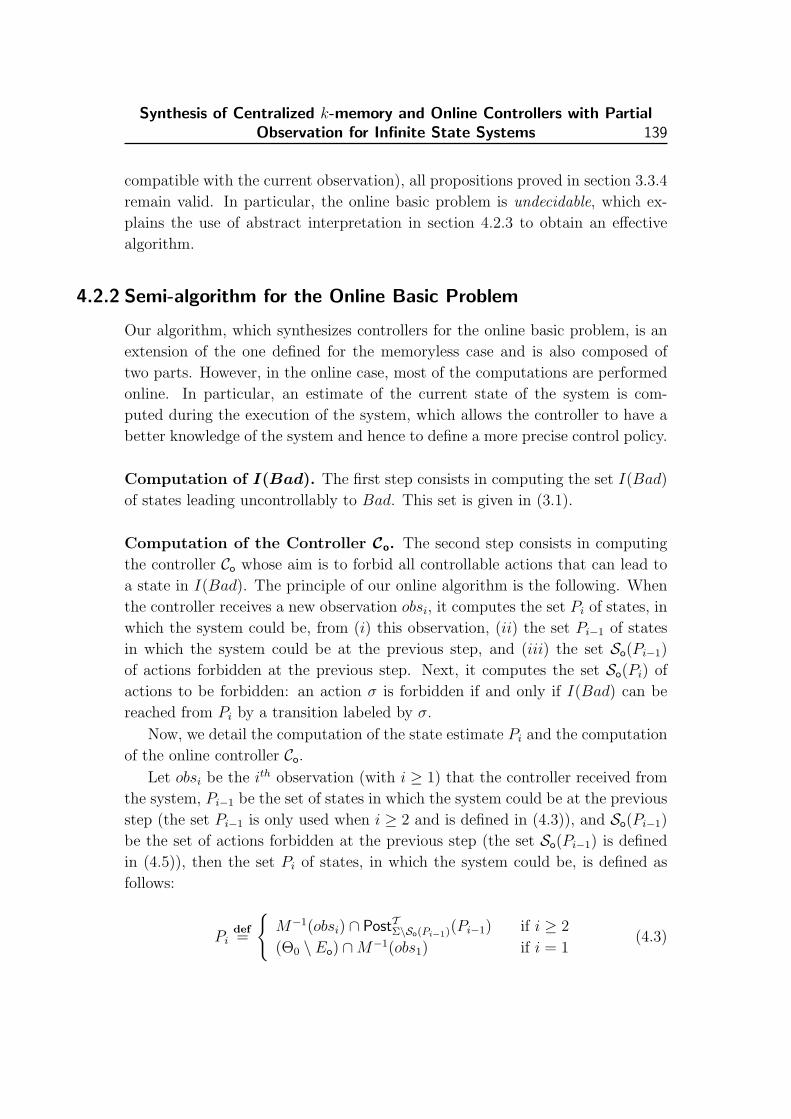
Synthesis of Centralized k-memory and Online Controllers with PartialObservation for Infinite State Systems 139
compatible with the current observation), all propositions proved in section 3.3.4
remain valid. In particular, the online basic problem is undecidable, which ex-
plains the use of abstract interpretation in section 4.2.3 to obtain an effective
algorithm.
4.2.2 Semi-algorithm for the Online Basic Problem
Our algorithm, which synthesizes controllers for the online basic problem, is an
extension of the one defined for the memoryless case and is also composed of
two parts. However, in the online case, most of the computations are performed
online. In particular, an estimate of the current state of the system is com-
puted during the execution of the system, which allows the controller to have a
better knowledge of the system and hence to define a more precise control policy.
Computation of I(Bad). The first step consists in computing the set I(Bad)
of states leading uncontrollably to Bad. This set is given in (3.1).
Computation of the Controller Co. The second step consists in computing
the controller Co whose aim is to forbid all controllable actions that can lead to
a state in I(Bad). The principle of our online algorithm is the following. When
the controller receives a new observation obsi, it computes the set Pi of states, in
which the system could be, from (i) this observation, (ii) the set Pi−1 of states
in which the system could be at the previous step, and (iii) the set So(Pi−1)
of actions forbidden at the previous step. Next, it computes the set So(Pi) of
actions to be forbidden: an action σ is forbidden if and only if I(Bad) can be
reached from Pi by a transition labeled by σ.
Now, we detail the computation of the state estimate Pi and the computation
of the online controller Co.Let obsi be the ith observation (with i ≥ 1) that the controller received from
the system, Pi−1 be the set of states in which the system could be at the previous
step (the set Pi−1 is only used when i ≥ 2 and is defined in (4.3)), and So(Pi−1)
be the set of actions forbidden at the previous step (the set So(Pi−1) is defined
in (4.5)), then the set Pi of states, in which the system could be, is defined as
follows:
Pidef=
{M−1(obsi) ∩ PostTΣ\So(Pi−1)(Pi−1) if i ≥ 2
(Θ0 \ Eo) ∩M−1(obs1) if i = 1(4.3)
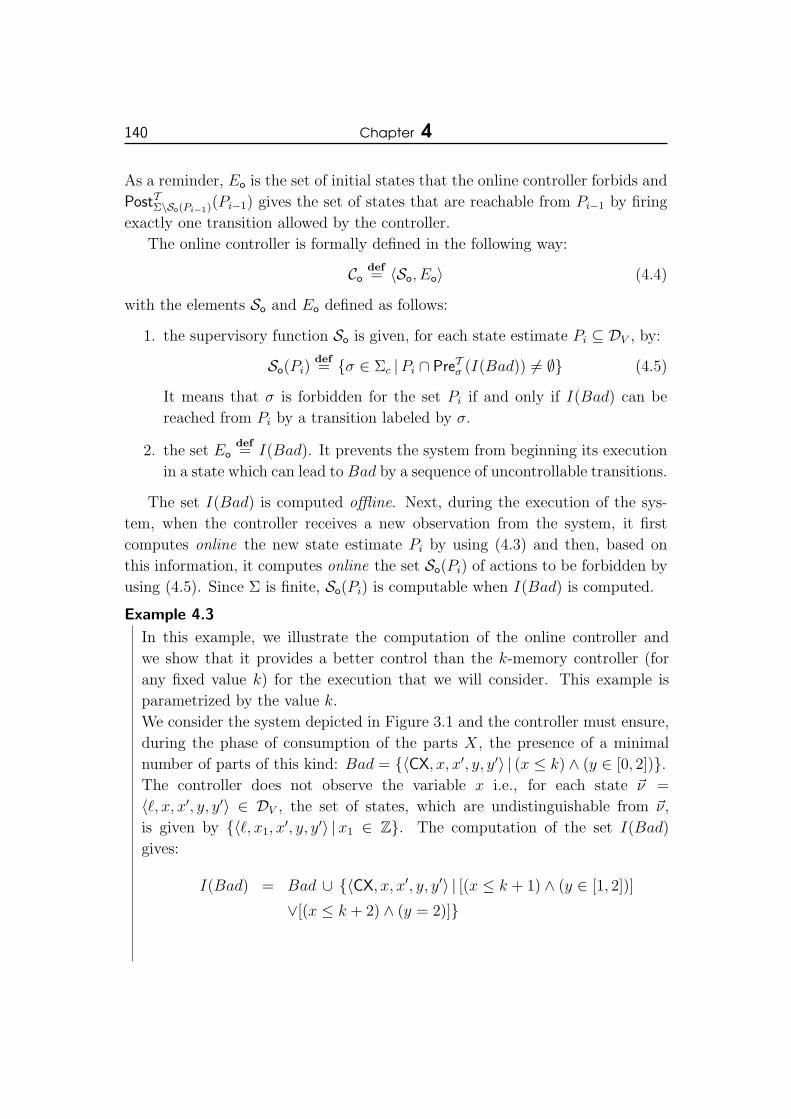
140 Chapter 4
As a reminder, Eo is the set of initial states that the online controller forbids and
PostTΣ\So(Pi−1)(Pi−1) gives the set of states that are reachable from Pi−1 by firing
exactly one transition allowed by the controller.
The online controller is formally defined in the following way:
Codef= 〈So, Eo〉 (4.4)
with the elements So and Eo defined as follows:
1. the supervisory function So is given, for each state estimate Pi ⊆ DV , by:
So(Pi)def= {σ ∈ Σc |Pi ∩ PreTσ (I(Bad)) 6= ∅} (4.5)
It means that σ is forbidden for the set Pi if and only if I(Bad) can be
reached from Pi by a transition labeled by σ.
2. the set Eodef= I(Bad). It prevents the system from beginning its execution
in a state which can lead to Bad by a sequence of uncontrollable transitions.
The set I(Bad) is computed offline. Next, during the execution of the sys-
tem, when the controller receives a new observation from the system, it first
computes online the new state estimate Pi by using (4.3) and then, based on
this information, it computes online the set So(Pi) of actions to be forbidden by
using (4.5). Since Σ is finite, So(Pi) is computable when I(Bad) is computed.
Example 4.3
In this example, we illustrate the computation of the online controller and
we show that it provides a better control than the k-memory controller (for
any fixed value k) for the execution that we will consider. This example is
parametrized by the value k.
We consider the system depicted in Figure 3.1 and the controller must ensure,
during the phase of consumption of the parts X, the presence of a minimal
number of parts of this kind: Bad = {〈CX, x, x′, y, y′〉 | (x ≤ k) ∧ (y ∈ [0, 2])}.The controller does not observe the variable x i.e., for each state ~ν =
〈`, x, x′, y, y′〉 ∈ DV , the set of states, which are undistinguishable from ~ν,
is given by {〈`, x1, x′, y, y′〉 |x1 ∈ Z}. The computation of the set I(Bad)
gives:
I(Bad) = Bad ∪ {〈CX, x, x′, y, y′〉 | [(x ≤ k + 1) ∧ (y ∈ [1, 2])]
∨[(x ≤ k + 2) ∧ (y = 2)]}

Synthesis of Centralized k-memory and Online Controllers with PartialObservation for Infinite State Systems 141
Let us consider the following execution: 〈Choice, 0, 0, 0, 0〉 δ9−→ 〈PX, 0, 0, 0, 0〉δ3−→ 〈PX, 1, 0, 0, 0〉 δ3−→ 〈PX, 2, 0, 0, 0〉 δ3−→ 〈PX, 3, 0, 0, 0〉 δ4−→ 〈CX, 3, 0, 2, 0〉 δ2−→〈Choice, 3, 0, 2, 0〉 δ9−→ 〈PX, 3, 0, 2, 0〉 δ3−→ 〈PX, 4, 0, 2, 0〉 δ3−→ . . .
δ3−→ 〈PX, k +
3, 0, 2, 0〉. At each step of this execution, the online controller computes an
estimate Pi which is equal to the current state. Thus, when the system
arrives in the state 〈PX, k + 3, 0, 2, 0〉, the controller computes an estimate
Pi = {〈PX, k + 3, 0, 2, 0〉} and it allows the action Stop prod, because this
action does not lead to a forbidden state from the state 〈PX, k + 3, 0, 2, 0〉.For the k-memory controller, when the system arrives in the
state 〈PX, k + 3, 0, 2, 0〉, the content of its memory is equal to
〈M(〈PX, 4, 0, 2, 0〉), . . . ,M(〈PX, k + 3, 0, 2, 0〉)〉. It then forbids the ac-
tion Stop prod, because the sequence of states 〈PX, 3, 0, 2, 0〉, . . . , 〈PX, k +
2, 0, 2, 0〉 leads to the forbidden state 〈CX, k + 2, 0, 2, 0〉 by
Stop prod and also 〈M(〈PX, 3, 0, 2, 0〉), . . . ,M(〈PX, k + 2, 0, 2, 0〉)〉 =
〈M(〈PX, 4, 0, 2, 0〉), . . . ,M(〈PX, k + 3, 0, 2, 0〉)〉. Thus, the online controller
is strictly more permissive than the k-memory controller for the sequence
considered in this example. In Proposition 4.5, we prove that it is always
more permissive than the k-memory controller.
The following property proves that our algorithm synthesizes correct controllers
for the online basic problem:
Proposition 4.2
Given an STS T = 〈V,Θ0,Σ,∆〉, an observer 〈Obs,M〉 and a predicate Bad,
which represents a set of forbidden states, the controller Co = 〈So, Eo〉, defined
by (4.4), solves the online basic problem (when Θ0 6⊆ Eo).
Proof
We prove by induction on the length n of the sequences of transitions (these
sequences begin in an initial state) that I(Bad) (and thus Bad) is not reachable
in the system T under the control of Co:
• Base case (n = 0): the execution of the system T under the control
of Co starts in a state which belongs to (Θ0 \ Eo) ∩M−1(obs1) = (Θ0 \I(Bad)) ∩M−1(obs1) (where obs1 is the first observation received from
the system). Thus, this system avoids I(Bad).

142 Chapter 4
• Induction step: we suppose that the proposition holds for the sequences
of transitions of length less than or equal to n and we prove that this
property remains true for the sequences of transitions of length n + 1.
The state estimate computed after a sequence of transitions of length
i (with i ≥ 0) is denoted by Pi+1. By induction hypothesis, each state
~ν1 reachable by a sequence of transitions of length n (thus ~ν1 ∈ Pn+1)
does not belong to I(Bad) and we have to show that each transition
δ = 〈σ,G,A〉 ∈ ∆, which can lead to a state ~ν2 ∈ I(Bad) from this state
~ν1 in the system T , cannot be fired from ~ν1 in the system T under the
control of Co. For that, we consider two cases :
• if δ ∈ ∆c, then this transition cannot be fired from ~ν1 in the system
T under the control of Co. Indeed, ~ν1 ∈ PreTσ (I(Bad)) (because ~ν1 ∈PreTσ (~ν2) and ~ν2 ∈ I(Bad)), which implies that σ ∈ So(Pn+1) (because
~ν1 ∈ (Pn+1 ∩ PreTσ (I(Bad)))).
• if δ ∈ ∆uc, then ~ν2 ∈ I(Bad) (by (3.1)), which is impossible by
hypothesis.
Hence, in the system T under the control of Co, the forbidden state ~ν2
cannot be reached from the state ~ν1 by the transition δ.
4.2.3 Effective Algorithm for the Online Basic Problem
As in chapter 3, an effective algorithm can be obtained by using abstract inter-
pretation techniques. For that, we first compute an overapproximation I ′(Bad)
of I(Bad) (see section 3.4.2 for the details). Next, we define our online controller
Co = 〈So, I′(Bad)〉 as in (4.4) by using I ′(Bad) and the state estimates P ]
i in-
stead of I(Bad) and Pi. The state estimates P ]i are obtained by transposing the
function (see (4.3)) defining Pi into the abstract lattice (thus the computation
of P ]i may require overapproximations).
4.3 Comparisons between the Memoryless, k-Memory
and Online Controllers
Up to now, we have proposed three different controllers for the basic problem:
the memoryless, k-memory, and online controllers. In this section, we theoret-
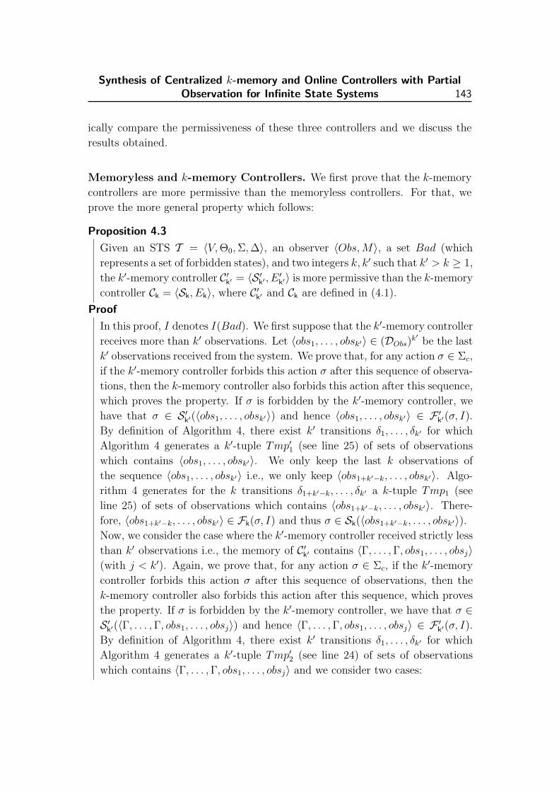
Synthesis of Centralized k-memory and Online Controllers with PartialObservation for Infinite State Systems 143
ically compare the permissiveness of these three controllers and we discuss the
results obtained.
Memoryless and k-memory Controllers. We first prove that the k-memory
controllers are more permissive than the memoryless controllers. For that, we
prove the more general property which follows:
Proposition 4.3
Given an STS T = 〈V,Θ0,Σ,∆〉, an observer 〈Obs,M〉, a set Bad (which
represents a set of forbidden states), and two integers k, k′ such that k′ > k ≥ 1,
the k′-memory controller C ′k′ = 〈S ′k′ , E ′k′〉 is more permissive than the k-memory
controller Ck = 〈Sk, Ek〉, where C ′k′ and Ck are defined in (4.1).
Proof
In this proof, I denotes I(Bad). We first suppose that the k′-memory controller
receives more than k′ observations. Let 〈obs1, . . . , obsk′〉 ∈ (DObs)k′ be the last
k′ observations received from the system. We prove that, for any action σ ∈ Σc,
if the k′-memory controller forbids this action σ after this sequence of observa-
tions, then the k-memory controller also forbids this action after this sequence,
which proves the property. If σ is forbidden by the k′-memory controller, we
have that σ ∈ S ′k′(〈obs1, . . . , obsk′〉) and hence 〈obs1, . . . , obsk′〉 ∈ F ′k′(σ, I).
By definition of Algorithm 4, there exist k′ transitions δ1, . . . , δk′ for which
Algorithm 4 generates a k′-tuple Tmp′1 (see line 25) of sets of observations
which contains 〈obs1, . . . , obsk′〉. We only keep the last k observations of
the sequence 〈obs1, . . . , obsk′〉 i.e., we only keep 〈obs1+k′−k, . . . , obsk′〉. Algo-
rithm 4 generates for the k transitions δ1+k′−k, . . . , δk′ a k-tuple Tmp1 (see
line 25) of sets of observations which contains 〈obs1+k′−k, . . . , obsk′〉. There-
fore, 〈obs1+k′−k, . . . , obsk′〉 ∈ Fk(σ, I) and thus σ ∈ Sk(〈obs1+k′−k, . . . , obsk′〉).Now, we consider the case where the k′-memory controller received strictly less
than k′ observations i.e., the memory of C ′k′ contains 〈Γ, . . . ,Γ, obs1, . . . , obsj〉(with j < k′). Again, we prove that, for any action σ ∈ Σc, if the k′-memory
controller forbids this action σ after this sequence of observations, then the
k-memory controller also forbids this action after this sequence, which proves
the property. If σ is forbidden by the k′-memory controller, we have that σ ∈S ′k′(〈Γ, . . . ,Γ, obs1, . . . , obsj〉) and hence 〈Γ, . . . ,Γ, obs1, . . . , obsj〉 ∈ F ′
k′(σ, I).
By definition of Algorithm 4, there exist k′ transitions δ1, . . . , δk′ for which
Algorithm 4 generates a k′-tuple Tmp′2 (see line 24) of sets of observations
which contains 〈Γ, . . . ,Γ, obs1, . . . , obsj〉 and we consider two cases:

144 Chapter 4
• either j < k: Algorithm 4 generates for the k transitions δ1+k′−k, . . . , δk′
a k-tuple Tmp2 (see line 24) of sets of observations which contains
〈Γ, . . . ,Γ, obs1, . . . , obsj〉. Therefore, 〈Γ, . . . ,Γ, obs1, . . . , obsj〉 ∈ Fk(σ, I)
and thus σ ∈ Sk(〈Γ, . . . ,Γ, obs1, . . . , obsj〉).• or j >= k: Algorithm 4 generates for the k transitions δ1+k′−k, . . . , δk′
a k-tuple Tmp1 (see line 25) of sets of observations which contains
〈obs1+j−k, . . . , obsj〉. Therefore, 〈obs1+j−k, . . . , obsj〉 ∈ Fk(σ, I) and thus
σ ∈ Sk(〈obs1+j−k, . . . , obsj〉).
Thus, increasing the size k of the memory of the k-memory controller gives a
more permissive solution, but it also increases the time complexity to compute
it. Indeed, Algorithm 4 enumerates all sequences of transitions of length k to
compute the function Fk and thus it enumerates |∆|k sequences. Therefore, when
the size k of the memory increases, the time complexity of Algorithm 4 also
increases. This proposition also holds when abstract interpretation techniques
are used to obtain effective algorithms. Indeed, we can remark that the proof
of this proposition remains correct when the overapproximations, induced by
abstract interpretation, are taken into account.
From Proposition 4.3, we can deduce the following property:
Proposition 4.4
Given an STS T = 〈V,Θ0,Σ,∆〉, an observer 〈Obs,M〉, a set Bad (which
represents a set of forbidden states), and an integer k ≥ 1, the k-memory con-
troller Ck = 〈Sk, Ek〉 (defined in (4.1)) is more permissive than the memoryless
controller C = 〈S, E〉 (defined in (3.3)).
Moreover, in Example 4.2, we shown that the k-memory controller (with k ≥ 2)
can be strictly more permissive than the memoryless controller.
Thus, the k-memory controller has a better control policy than the memory-
less controller. However, it requires additional offline computations to compute
the function Fk. Indeed, as explained above, the time complexity of the compu-
tation of Fk increases when k increases. Similarly, for the online part of these
methods, the membership test of the k-memory controller has a greater time
complexity than the one of the memoryless controller (it is k times greater).
The choice between these two controllers thus depends on the requirements of
the user. The k-memory controller must be used when the aim is to obtain a
solution of better quality and the memoryless controller must be used when the

Synthesis of Centralized k-memory and Online Controllers with PartialObservation for Infinite State Systems 145
purpose is to quickly compute a solution.
k-Memory and Online Controllers. Now, we prove that the online controllers
are more permissive than the k-memory controllers:
Proposition 4.5
Given an STS T = 〈V,Θ0,Σ,∆〉, an observer 〈Obs,M〉, a set Bad (which
represents a set of forbidden states), and an integer k ≥ 1, the online con-
troller Co = 〈So, Eo〉 (defined in (4.4)) is more permissive than the k-memory
controller Ck = 〈Sk, Ek〉 (defined in (4.1)).
Proof
In this proof, I denotes I(Bad). Let obs1, . . . , obsj be the sequence of obser-
vations received by the controllers from the system since the beginning of the
execution of the system. By Proposition 4.2, we have, for each i ∈ [1, j], that:
Pi ∩ I(Bad) = ∅ (4.6)
where Pi (∀i ≥ 1) denotes the state estimate computed by Co after the reception
of the observation obsi.
We prove that, for any action σ ∈ Σc, if the online controller forbids this
action σ after the sequence obs1, . . . , obsj of observations, then the k-memory
controller also forbids this action after this sequence, which proves the prop-
erty.
We first consider the case where j ≥ k. We suppose that σ is forbidden
by the online controller after the sequence obs1, . . . , obsj and we have then
that σ ∈ So(Pj). We will prove that there exist k transitions δ1, . . . , δk (with
δk ∈ Trans(σ)) for which Algorithm 4 generates a k-tuple Tmp1 (line 25) of
sets of observations that contains 〈obsj−k+1, . . . , obsj〉. First, we prove that
obsj ∈ Tmp1
⌋[k]
:
σ ∈ So(Pj)
⇒ Pj ∩ PreTσ (I) 6= ∅, by (4.5)
⇒ ∃~ν1 ∈ Pj,∃δk ∈ Trans(σ) : ~ν1 ∈ PreTδk(I)
⇒ ∃~ν1 ∈ Pj,∃δk ∈ Trans(σ) : ~ν1 ∈ (PreTδk(I) \ I), because ~ν1 6∈ I
by (4.6) (α)
⇒ obsj ∈M(PreTδk(I) \ I), because obsj ∈M(~ν1) by (4.3)
⇒ obsj ∈ Tmp1
⌋[k], by definition of Tmp1 in Algorithm 4
146 Chapter 4
Next, we prove that obsj−1 ∈ Tmp1
⌋[k−1]
. By (α), we know that ∃~ν1 ∈Pj,∃δk ∈ Trans(σ) : ~ν1 ∈ (PreTδk
(I) \ I) and, by reasoning on this state ~ν1,
we can deduce the following information:
~ν1 ∈ Pj
⇒ ~ν1 ∈ PostTΣ\So(Pj−1)(Pj−1), by (4.3)
⇒ ∃~ν2 ∈ Pj−1 : ~ν1 ∈ PostTΣ\So(Pj−1)(~ν2)
⇒ ∃~ν2 ∈ Pj−1 : ~ν1 ∈ PostTΣ(~ν2), because Σ \ So(Pj−1) ⊆ Σ
⇒ ∃~ν2 ∈ Pj−1 : ~ν2 ∈ PreTΣ(~ν1)
⇒ ∃~ν2 ∈ Pj−1,∃δk−1 ∈ ∆ : ~ν2 ∈ PreTδk−1(~ν1), because δk−1 ∈ Trans(Σ)
⇒ ∃~ν2 ∈ Pj−1,∃δk−1 ∈ ∆ : ~ν2 ∈ PreTδk−1(PreTδk
(I) \ I), because
~ν1 ∈ (PreTδk(I) \ I) by (α).
⇒ ∃~ν2 ∈ Pj−1,∃δk−1 ∈ ∆ : ~ν2 ∈ (PreTδk−1(PreTδk
(I) \ I) \ I), because
~ν2 6∈ I by (4.6) (β)
⇒ obsj−1 ∈M(PreTδk−1(PreTδk
(I) \ I) \ I), because obsj−1 ∈M(~ν2)
by (4.3)
⇒ obsj−1 ∈ Tmp1
⌋[k−1]
, by definition of Tmp1 in Algorithm 4
By (β), we know that ∃~ν2 ∈ Pj−1,∃δk−1 ∈ ∆ : ~ν2 ∈ (PreTδk−1(PreTδk
(I) \ I) \ I)and we can prove similarly as above that (i) obsj−2 ∈ Tmp1
⌋[k−2]
and (ii) ∃~ν3 ∈Pj−2,∃δk−2 ∈ ∆ : ~ν3 ∈ [PreTδk−2
(PreTδk−1(PreTδk
(I) \ I) \ I) \ I]. Then, with the
same reasoning, we prove that obsj−i ∈ Tmp1
⌋[k−i]
and ∃~νi+1 ∈ Pj−i,∃δk−i ∈∆ : ~νi+1 ∈ [PreTδk−i
(. . . (PreTδk(I) \ I) . . .) \ I] (for i = 3, 4, . . . , k − 1). Thus,
we have proven that obsj−i ∈ Tmp1
⌋[k−i]
(∀i ∈ [0, k − 1]). Therefore, the last
k observations obsj−k+1, . . . , obsj of the sequence obs1, . . . , obsj are such that
〈obsj−k+1, . . . , obsj〉 ∈ Tmp1 and thus 〈obsj−k+1, . . . , obsj〉 ∈ Fk(σ, I(Bad)) (by
definition of Fk). This implies that σ ∈ Sk(〈obsj−k+1, . . . , obsj〉). The action σ
is thus forbidden by the k-memory controller after the sequence obs1, . . . , obsj.
For the case where j < k, we can prove as above that σ ∈Sk(〈Γ, . . . ,Γ, obs1, . . . , obsj〉).
Moreover, in Example 4.3, we showed that the online controller can be strictly
more permissive than the k-memory controller.
The online controller has a better control policy than the k-memory controller
Synthesis of Centralized k-memory and Online Controllers with PartialObservation for Infinite State Systems 147
and its offline part requires less computations than the one of the k-memory con-
troller. However, it requires significant online computations to choose the actions
to be forbidden. Indeed, the online part of the k-memory method only requires
a membership test (see (4.2)), whereas the one of the online method requires
the computation of several operations having a polynomial time complexity4
(see (4.3) and (4.5)). In particular, if the time to choose the actions to be for-
bidden is short, we will not always be able to use the online controller. We must
then use the k-memory controller or the memoryless controller.
Unfortunately, our approach, based on abstract interpretation, does not
ensure the validity of this proposition since the algorithms, which synthesize
the online and k-memory controllers, are quite different. So, if, for example,
our effective online algorithm computes rough state estimates (e.g., Pi = DV )
and our effective k-memory algorithm does not use overapproximations in
its computations, then our online controller will be less permissive than our
k-memory controller.
Full Observation. Under full observation (that corresponds to the case where
DObs = DV and M = IdDV), we have that the memoryless, k-memory and online
controllers have the same permissiveness.
Proposition 4.6
Given an STS T = 〈V,Θ0,Σ,∆〉, an observer 〈Obs,M〉 (where DObs = DV
and M = IdDV), a set Bad (which represents a set of forbidden states), and
an integer k ≥ 1, the memoryless controller C = 〈S, E〉 (defined in (3.3)), the
k-memory controller Ck = 〈Sk, Ek〉 (defined in (4.1)) and the online controller
Co = 〈So, Eo〉 (defined in (4.4)) have the same permissiveness.
Proof
We first prove that the memoryless and online controllers have the same per-
missiveness. For these two controllers, the computation of the set I(Bad) gives
the same result. Next, when the system arrives in a state ~ν, the memoryless
controller receives this state as information and it forbids the set S(~ν) of ac-
tions. By (3.4), this set S(~ν) = {σ ∈ Σc |~ν ∈ (PreTσ (I(Bad)) \ I(Bad))} i.e.,
the memoryless controller forbids an action σ in the state ~ν if there exists a
4More precisely, the online part of the online method requires to compute set intersections,set differences and the functions Post, Pre and M−1. These operations can be computed inpolynomial time.

148 Chapter 4
transition labeled by σ which leads to I(Bad) from ~ν. When the online con-
troller receives the information ~ν from the system, it computes a state estimate
Pi = {~ν} and it forbids the set So(~ν) of actions. This set So(~ν) = S(~ν), be-
cause:
So(~ν) = {σ ∈ Σc | {~ν} ∩ PreTσ (I(Bad)) 6= ∅}, by (4.5)
= {σ ∈ Σc |~ν ∈ PreTσ (I(Bad))}= {σ ∈ Σc |~ν ∈ (PreTσ (I(Bad)) \ I(Bad))}, because ~ν 6∈ I(Bad)
by Proposition 4.2
= S(~ν)
Thus, the memoryless and online controllers have the same control policy and
hence they have the same permissiveness.
This property, Proposition 4.4 (i.e., C �p Ck), and Proposition 4.5 (i.e.,
Ck �p Co) imply that the memoryless and k-memory controllers have the same
permissiveness.
In conclusion, we have proven that the memoryless, k-memory, and online
controllers have the same permissiveness.
Consequently, when the system is perfectly observed, it is preferable to
synthesize a memoryless controller.
One can note that this proposition remains valid in our approach based on
abstract interpretation.

Chapter
5Synthesis of Decentralized and
Modular Controllers for Infinite
State Systems
In chapters 3 and 4, we were interested in the centralized control of
infinite state systems (i.e., a single controller interacts with the system
in order to restrict its behavior). However, in some cases, the nature
of the system to be controlled makes unrealistic the use of such an approach
(e.g., distributed systems). The decentralized framework is an alternative to the
centralized framework and is more suitable for the control of distributed systems
with synchronous communications. This framework has widely been studied in
the past years and has shown its usefulness in several domains like manufacturing
systems, communication network protocols, . . . [RW92a]. In this approach, n
local controllers interact with the system in a feedback manner to satisfy some
control objectives. Each local controller has its own view of the system and its
own set of controllable actions. Indeed, due to the distributed nature of the
system to be controlled, the controllers observe the system through different sets
of sensors (these sets can overlap) and control it by means of different sets of
actuators (these sets can also overlap). Moreover, one supposes the existence of a
coordination mechanism to define the global control to be applied to the system:
each local controller defines its own set of actions to be forbidden (based on its

150 Chapter 5
own view of the system) and the global control applied to the system is defined
by a fusion rule which depends on the actions forbidden by each controller.
As explained above, the decentralized control is suitable for the control of
distributed systems with synchronous communications, but it has also other ad-
vantages. It decreases the computational complexity of synthesizing controllers,
because the overal task of synthesis is divided into synthesizing local controllers.
It also provides more flexibility. Indeed, if a sensor must be replaced (because of
a failure for example), only the controllers, which use it, must be recomputed.
In the decentralized framework, we have generally no information regarding
the structure of the distributed system to be controlled while the computation
of the controllers, which implies that these computations are performed on the
model of the global system. However, if this structure is known and if the system
is composed of several subsystems acting in parallel, it is of interest to exploit
this knowledge to compute the set of controllers ensuring the expected properties
without having to compute the model of the global system. Indeed, in this way,
the classical problem of the state space explosion inherent to the parallel compo-
sition of subsystems is avoided. This might also have an impact when performing
some fixpoint computations that are necessary to calculate the set of states that
have to be avoided. In the sequel, this particular framework is called modular
framework as opposed to the decentralized framework for which the structure of
the system is not taken into account when performing the computation of the
controllers.
The remainder of this chapter is structured as follows. First, in section 5.1,
we define an algorithm which synthesizes decentralized controllers for the state
avoidance control problem by using techniques similar to the ones used in chap-
ters 3 and 4. Next, in section 5.2, we turn our attention to the modular approach
and we define an algorithm synthesizing controllers for the state avoidance con-
trol problem. Finally, in section 5.3, we experimentally evaluate our methods.
5.1 Synthesis of Decentralized Controllers
In this section, we define an algorithm which synthesizes controllers for the state
avoidance control problem in the decentralized framework.
The remainder of this chapter is structured as follows. First, in section 5.1.1,
we formally define the decentralized framework and the problems that we want
to solve. Next, in section 5.1.2, we propose an algorithm which synthesizes
controllers for the state avoidance control problem. In section 5.1.3, we extend

Synthesis of Decentralized and Modular Controllers for Infinite StateSystems 151
this algorithm to the deadlock free case. Finally, in section 5.1.4, we theoretically
compare the permissiveness of our centralized and decentralized controllers.
5.1.1 Framework and State Avoidance Control Problem
The system to be controlled is given by an STS. This system is controlled by
n local controllers; each local controller has its own view of the system and its
own set of controllable actions. The global control applied to T is given by a
fusion rule, which depends on the set of actions forbidden by each local controller.
Means of Observation. In the decentralized framework, each local controller
Ci (∀i ∈ [1, n]) has its own partial view of the state space of the system, which is
modeled by an observer (see Definition 3.8). Therefore, an observer 〈Obsi,Mi〉is associated with each controller Ci and when the system arrives in a state ~ν,
the controller Ci receives an observation obsi ∈Mi(~ν).
Remark 5.1
For more conciseness, we suppose throughout this chapter that the masks Mi
correspond to partitions of the state space, but the results, that we present,
also hold when the masks Mi correspond to coverings.
Means of Control. Each local controller Ci (∀i ∈ [1, n]) interacts with the
system in a feedback manner: it receives an observation from the system and
defines, from this information, a set of actions that it proposes to forbid. In
this mechanism, the set of actions Σ is partitioned, for each controller Ci, into
the set of controllable actions Σi,c, that can be forbidden by Ci, and the set
of uncontrollable actions Σi,uc, that cannot be forbidden by Ci. The subsets
Σ1,c, . . . ,Σn,c are not necessarily disjoint. The set of actions that can be controlled
by at least one controller is denoted by Σc and is defined by Σcdef=⋃n
i=1 Σi,c and
the set of actions that cannot be controlled is denoted by Σuc and is defined
by Σucdef= Σ \ Σc. That also induces a partition of the set of transitions ∆
into the set ∆c (resp. ∆i,c) and the set ∆uc (resp. ∆i,uc) in the following way:
〈σ,G,A〉def∈ ∆c (resp. ∆i,c) if σ ∈ Σc (resp. Σi,c), and 〈σ,G,A〉
def∈ ∆uc (resp.
∆i,uc) if σ ∈ Σuc (resp. Σi,uc).
In the sequel, we use the function In : Σ → 2{1,...,n} which gives, for each
action σ ∈ Σ, the set of indices of the controllers that control σ i.e., In(σ)def=
{i |σ ∈ Σi,c}.

152 Chapter 5
Decentralized Controller and Controlled System. A local controller has
the possibility to forbid some actions and the aim is to restrict the behavior of
the system by combining the control decisions of the n local controllers in order
to ensure the desired property.
The formal definition of a local controller is given in Definition 3.9. The global
control applied to the system is defined by a fusion rule which gives the actions
and the initial states to be forbidden and which depends on the control decisions
of each local controller. Within our framework, a fusion rule is formally defined
as follows:
Definition 5.1 (Fusion Rule)
Given an STS T = 〈V,Θ0,Σ,∆〉, n observers 〈Obsi,Mi〉 (∀i ∈ [1, n]) and n
controllers Ci = 〈Si, Ei〉 (∀i ∈ [1, n]), a fusion rule for the actions and the
initial states to be forbidden is a pair R def= 〈RS ,RE〉, where:
• the function RS : 2Σ1,c × . . . × 2Σn,c → 2Σc gives, for each set Bi ⊆Σi,c (∀i ∈ [1, n]) of controllable actions that Ci proposes to forbid, the
set RS(B1, . . . , Bn) of actions that the system cannot fire. Thus, this
function defines the global control to be applied to the system by giving
the actions that are effectively forbidden.
• the function RE : 2DV × . . . × 2DV → 2DV gives, for each set Ei ⊆ DV
(∀i ∈ [1, n]) of states that Ci proposes to forbid at the beginning of
the execution of the system, the set RE(E1, . . . , En) of states that are
effectively forbidden.
We explain further how we instantiate the fusion ruleR. Based on Definitions 3.9
and 5.1, a decentralized controller is defined as follows:
Definition 5.2 (Decentralized Controller)
Given an STS T = 〈V,Θ0,Σ,∆〉, and n observers 〈Obsi,Mi〉 (∀i ∈ [1, n]), a
decentralized controller is defined by n local controllers Ci (∀i ∈ [1, n]) coordi-
nated by a fusion rule R and is formally given by a pair 〈(Ci)ni=1,R〉, where:
• Ci = 〈Si, Ei〉 (∀i ∈ [1, n]) is a local controller (see Definition 3.9) defined
w.r.t. (i) the observer 〈Obsi,Mi〉, (ii) the set of controllable actions Σi,c,
and (iii) the set of uncontrollable actions Σi,uc.
• R is a fusion rule (see Definition 5.1).
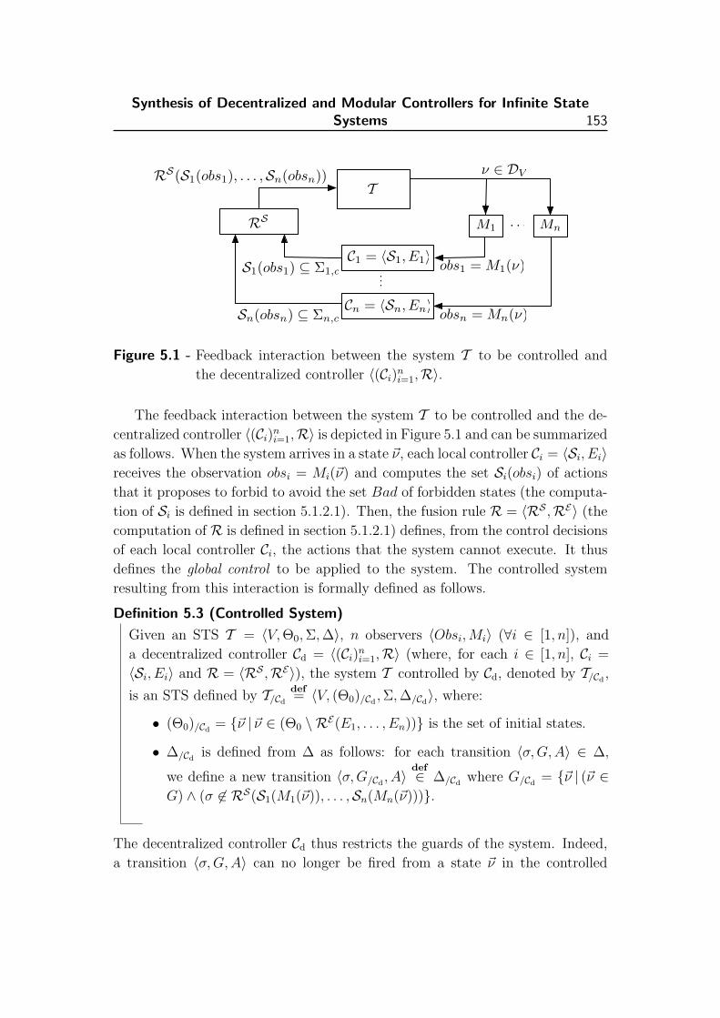
Synthesis of Decentralized and Modular Controllers for Infinite StateSystems 153
T
MnM1 . . .
C1 = 〈S1, E1〉
Cn = 〈Sn, En〉
ν ∈ DV
...
RS
obs1 = M1(ν)
obsn = Mn(ν)Sn(obsn) ⊆ Σn,c
S1(obs1) ⊆ Σ1,c
RS(S1(obs1), . . . ,Sn(obsn))
Figure 5.1 - Feedback interaction between the system T to be controlled and
the decentralized controller 〈(Ci)ni=1,R〉.
The feedback interaction between the system T to be controlled and the de-
centralized controller 〈(Ci)ni=1,R〉 is depicted in Figure 5.1 and can be summarized
as follows. When the system arrives in a state ~ν, each local controller Ci = 〈Si, Ei〉receives the observation obsi = Mi(~ν) and computes the set Si(obsi) of actions
that it proposes to forbid to avoid the set Bad of forbidden states (the computa-
tion of Si is defined in section 5.1.2.1). Then, the fusion rule R = 〈RS ,RE〉 (the
computation of R is defined in section 5.1.2.1) defines, from the control decisions
of each local controller Ci, the actions that the system cannot execute. It thus
defines the global control to be applied to the system. The controlled system
resulting from this interaction is formally defined as follows.
Definition 5.3 (Controlled System)
Given an STS T = 〈V,Θ0,Σ,∆〉, n observers 〈Obsi,Mi〉 (∀i ∈ [1, n]), and
a decentralized controller Cd = 〈(Ci)ni=1,R〉 (where, for each i ∈ [1, n], Ci =
〈Si, Ei〉 and R = 〈RS ,RE〉), the system T controlled by Cd, denoted by T/Cd,
is an STS defined by T/Cd
def= 〈V, (Θ0)/Cd
,Σ,∆/Cd〉, where:
• (Θ0)/Cd= {~ν |~ν ∈ (Θ0 \ RE(E1, . . . , En))} is the set of initial states.
• ∆/Cdis defined from ∆ as follows: for each transition 〈σ,G,A〉 ∈ ∆,
we define a new transition 〈σ,G/Cd, A〉
def∈ ∆/Cd
where G/Cd= {~ν | (~ν ∈
G) ∧ (σ 6∈ RS(S1(M1(~ν)), . . . ,Sn(Mn(~ν)))}.
The decentralized controller Cd thus restricts the guards of the system. Indeed,
a transition 〈σ,G,A〉 can no longer be fired from a state ~ν in the controlled
154 Chapter 5
system, if the action σ is forbidden by the fusion rule.
Definition of the State Avoidance Decentralized Control Problem. We
define two distinct versions of the state avoidance control problem adapted to
the decentralized framework:
Problem 5.1 (Basic Decentralized Problem)
Given an STS T = 〈V,Θ0,Σ,∆〉, n observers 〈Obsi,Mi〉 (∀i ∈ [1, n]),
and a set Bad of forbidden states, the basic decentralized problem con-
sists in computing a decentralized controller Cd = 〈(Ci)ni=1,R〉 such that (i)
ReachableT/Cd∆/Cd
((Θ0)/Cd) 6= ∅ and (ii) Reachable
T/Cd∆/Cd
((Θ0)/Cd) ∩Bad = ∅.
This problem thus consists in synthesizing a non-trivial and valid decentralized
controller.
We are also interested in a second problem where the deadlock free property
is ensured:
Problem 5.2 (Deadlock Free Decentralized Problem)
Given an STS T = 〈V,Θ0,Σ,∆〉, n observers 〈Obsi,Mi〉 (∀i ∈ [1, n]), and
a set Bad of forbidden states, the deadlock free decentralized problem con-
sists in computing a decentralized controller Cd = 〈(Ci)ni=1,R〉 such that (i)
ReachableT/Cd∆/Cd
((Θ0)/Cd) 6= ∅, (ii) Reachable
T/Cd∆/Cd
((Θ0)/Cd) ∩ Bad = ∅, and (iii)
T/Cdis deadlock free.
The decentralized controller Cd must thus be (i) non-trivial and (ii) valid, and
(iii) it must define a deadlock free controlled system.
We extend the concept of permissiveness (see Definition 3.12) to the decen-
tralized framework in order to compare the quality of the different solutions of
a given problem:
Definition 5.4 (Permissiveness)
Given an STS T = 〈V,Θ0,Σ,∆〉 and n observers 〈Obsi,Mi〉 (∀i ∈ [1, n]),
a decentralized controller Cd = 〈(Ci)ni=1,R〉 is more permissive than a de-
centralized controller C ′d = 〈(C ′i)ni=1,R′〉 (denoted by C ′d �d
p Cd) if and only if
ReachableT/C′
d∆/C′
d
((Θ0)/C′d) ⊆ ReachableT/Cd∆/Cd
((Θ0)/Cd). When the inclusion is strict,
we say that Cd is strictly more permissive than C ′d (denoted by C ′d ≺dp Cd).
Since the centralized control is a particular case of the decentralized control
(it corresponds to the case where n is equal to 1), all results proved in sec-

Synthesis of Decentralized and Modular Controllers for Infinite StateSystems 155
tion 3.3.4 remain valid for the decentralized framework; in particular, computing
a decentralized controller for the basic or deadlock free decentralized problem is
undecidable. Therefore, we still use abstract interpretation techniques to define
effective algorithms for these problems.
5.1.2 Computation by Means of Abstract Interpretation of a Decen-
tralized Controller for the Basic Decentralized Problem
In this section, we define our algorithm which synthesizes decentralized con-
trollers for the basic decentralized problem. First, we present a semi-algorithm
for this problem and next, we explain how to extend it by using abstract inter-
pretation techniques to obtain an effective algorithm.
5.1.2.1 Semi-Algorithm for the Basic Decentralized Problem
Our algorithm, which computes decentralized controllers for the basic decentral-
ized problem, is a generalization of the algorithm defined in section 3.4 for the
centralized case. It is composed of two parts:
• we compute, using a fixpoint equation, the set I(Bad) of states leading un-
controllably to Bad.
• we compute the decentralized controller Cd. Each local controller of Cd forbids,
for each observation, the controllable actions that lead to I(Bad) from a state
compatible with this observation.
These two steps are detailed below.
Computation of I(Bad). The set I(Bad) of states leading uncontrollably
to Bad is given by the fixpoint equation defined in (3.1) which, as a reminder,
is equal to lfp⊆(λB.Bad ∪ PreT∆uc(B)). This fixpoint equation is used for the
computations of the n local controllers Ci and of the fusion rule R.
Computation of the Decentralized Controller Cd. First, we detail the
computation of the n local controllers Ci and next, we explain how to compute
the fusion rule R = 〈RS ,RE〉.The computation of the local controllers Ci is quite similar to the computation
of the centralized controller defined in section 3.4 for the basic problem. More
precisely, we first define, for each controller Ci (∀i ∈ [1, n]), the function Fi :

156 Chapter 5
Σ× 2DV → 2DObsi that gives, for each action σ ∈ Σ and for each set B ⊆ DV of
states to be forbidden, the set Fi(σ,B) of observations, for which the controller
Ci proposes to forbid the action σ. This set Fi(σ,B) actually corresponds to the
greatest set Oi ⊆ DObsiof observations such that, for each observation obs ∈ Oi,
there exists a state ~ν ∈ DV (with obs = Mi(~ν)) which leads to B by a transition
labeled by σ:
Fi(σ,B)def=
{Mi(PreTσ (B) \B) if σ ∈ Σi,c
∅ otherwise(5.1)
Next, each local controller Ci (∀i ∈ [1, n]) is defined, from its function Fi, in the
following way:
Cidef= 〈Si, Ei〉 (5.2)
where (i) the supervisory function Si is defined, for each obs ∈ DObsi, by
Si(obs)def= {σ ∈ Σi,c | obs ∈ Fi(σ, I(Bad))}, and (ii) the set Ei
def= I(Bad).
Then, the fusion rule R, which defines the global control to be applied to
the system, is defined from the control decisions of each local controller Ci in the
following way:
R def= 〈RS ,RE〉 (5.3)
where the elements RS and RE are defined as follows:
• Let Bi ⊆ Σi,c (∀i ∈ [1, n]) be the set of actions that the local controller Ciproposes to forbid, the function RS , which gives the set of actions that the
system cannot execute, is defined in the following way:
RS(B1, . . . , Bn)def= {σ ∈ Σc | ∀i ∈ In(σ) : σ ∈ Bi} (5.4)
Thus, an action σ cannot be executed by the system, if each local controller,
which controls this action, proposes to forbid it. Usually, one uses a conjunc-
tive or disjunctive architecture as defined in [RW92b, YL02] i.e., an action is
globally enabled when all local controllers enable it (conjunctive architecture)
or at least one local controller enables it (disjunctive architecture). In our
framework, an action is enabled whenever at least one local controller, that
controls this action, enables it. So, we use a variant of the disjunctive archi-
tecture. We will prove that our fusion rule defines correct solutions for the
basic and deadlock free decentralized problems (see Propositions 5.1 and 5.3),
whereas a disjunctive architecture does not always give correct solutions for

Synthesis of Decentralized and Modular Controllers for Infinite StateSystems 157
these problems (see Example 5.1). In [TKU94], which is one of the few pa-
pers on the decentralized control of discrete event systems with a state-based
approach, the authors use a conjunctive architecture to synthesize a decen-
tralized controller that allows the system to exactly reach a set Q of good
states. However, they want to obtain a balanced decentralized controller (i.e.,
for each pair of states ~ν, ~ν ′ reachable in the controlled system, if there is an
action σ which can be fired from ~ν to ~ν ′, then this action must be enabled
by each local controller). We do not ensure that our decentralized controllers
are balanced, since �p-maximal decentralized controllers do not always satisfy
this property (see Example 5.1).
• Let Ei ⊆ DV (∀i ∈ [1, n]) be the set of states that the local controller Ciproposes to forbid at the beginning of the execution of the system, the function
RE , which gives the set of states that must effectively be forbidden, is defined
as follows:
RE(E1, . . . , En)def=
n⋂i=1
Ei (5.5)
A state ~ν ∈ DV is thus forbidden at the beginning of the execution of the
system, if each local controller Ci proposes to forbid it.
Finally, the decentralized controller Cd is defined by the n local controllers Cigiven in (5.2) and by the fusion rule R given in (5.3):
Cddef= 〈(Ci)n
i=1,R〉 (5.6)
The set I(Bad) and the functions Fi (∀i ∈ [1, n]) are computed offline. Next,
during the execution of the system, when the system arrives in a state ~ν ∈ DV ,
each local controller Ci (∀i ∈ [1, n]) receives the observation obsi = Mi(~ν) ∈DObsi
and computes online the set Si(obsi) of actions that it proposes to forbid.
The fusion rule RS(S1(obs1), . . . ,Sn(obsn)) is then computed online from these
control decisions to obtain the set of actions that the system cannot execute.
Example 5.1
We compute a decentralized controller Cd = 〈〈C1, C2〉,R〉 for the system de-
picted in Figure 3.1.
The controller C1 has a partial observation modeled by the mask M1 : Loc ×Z4 → 2Loc×Z4
where, for each state ~ν = 〈`, x, x′, y, y′〉 ∈ DV , the set of states,
that are undistinguishable from ~ν, is given by {〈`, x, x′1, y, y′1〉 |x′1, y′1 ∈ Z} (i.e.,
C1 does not observe the variables x′ and y′). C1 does not control the actions
Cons, Cons′, Stop prod′ (i.e., Σ1,uc = {Cons, Cons′, Stop prod′}).

158 Chapter 5
The controller C2 has a partial observation modeled by the mask M2 : Loc ×Z4 → 2Loc×Z4
where, for each state ~ν = 〈`, x, x′, y, y′〉 ∈ DV , the set of states,
that are undistinguishable from ~ν, is given by {〈`, x1, x′, y1, y
′〉 |x1, y1 ∈ Z}(i.e., C2 does not observe the variables x and y). C2 does not control the actions
Cons, Cons′ (i.e., Σ2,uc = {Cons, Cons′}). The decentralized controller must
ensure, during the phase of consumption of the parts X and X ′, the presence
of a minimal number of parts: Bad = {〈CX, x, x′, y, y′〉 | (x ≤ 10) ∧ (y ∈[0, 2])} ∪ {〈CX′, x, x′, y, y′〉 | (x′ ≤ 10) ∧ (y′ ∈ [0, 2])}. The computation of the
set I(Bad) gives:
I(Bad) = Bad ∪ {〈CX, x, x′, y, y′〉 | [(x ≤ 11) ∧ (y ∈ [1, 2])] ∨ [(x ≤ 12)
∧(y = 2)]} ∪ {〈CX′, x, x′, y, y′〉 | [(x′ ≤ 11) ∧ (y′ ∈ [1, 2])] ∨[(x′ ≤ 12) ∧ (y′ = 2)]}
The computation of the function F1 gives:
F1(σ, I(Bad)) =
{M1({〈PX, x, x′, y, y′〉 |x ≤ 12}) if σ = Stop prod
∅ otherwise
The supervisory function S1 thus forbids the action Stop prod when the system
is in a state ~ν ∈ {〈PX, x, x′, y, y′〉 |x ≤ 12} and the computation of the function
F2 gives:
F2(σ, I(Bad)) =
M2({〈PX, x, x′, y, y′〉 |x ≤ 12}) if σ = Stop prod
M2({〈PX′, x, x′, y, y′〉 |x′ ≤ 12}) if σ = Stop prod′
∅ otherwise
Thus, the supervisory function S2 forbids the action Stop prod′ when the sys-
tem is in a state ~ν ∈ {〈PX′, x, x′, y, y′〉 |x′ ≤ 12} and it always forbids the
action Stop prod in the location PX. According to the fusion rule R, the de-
centralized controller Cd forbids the action Stop prod (resp. Stop prod′) in
the location PX (resp. PX′) when x ≤ 12 (resp. x′ ≤ 12). Note that Cd is
�p-maximal.
One can note that with a disjunctive architecture, the decentralized controller
always allows the action Stop prod′ in the location PX′, because the local
controller C1 always allows this action in PX′ (Stop prod′ ∈ Σ1,uc). Therefore,
Bad is reachable with a disjunctive architecture. Moreover, the decentralized
controller Cd, which is �p-maximal, is not balanced. Indeed, in the controlled
system T/Cd, the state ~ν = 〈CX, 50, 50, 2, 1〉 is reachable from the state ~ν ′ =
〈PX, 50, 50, 0, 1〉 by the action Stop prod, but this action is forbidden by C2 in
Synthesis of Decentralized and Modular Controllers for Infinite StateSystems 159
the state ~ν ′, whereas it is allowed by C1 in this state.
The following property proves that our algorithm synthesizes correct con-
trollers for the basic decentralized problem:
Proposition 5.1
Given an STS T = 〈V,Θ0,Σ,∆〉, n observers 〈Obsi,Mi〉 (∀i ∈ [1, n]) and a
predicate Bad, which represents a set of forbidden states, the decentralized
controller Cd = 〈(Ci)ni=1,R〉 (where, for each i ∈ [1, n], Ci = 〈Si, Ei〉 and
R = 〈RS ,RE〉), defined in (5.6), solves the basic decentralized problem (when
Θ0 6⊆ RE(E1, . . . , En)).
Proof
We prove by induction on the length ` of the sequences of transitions (these
sequences begin in an initial state) that ReachableT/Cd∆/Cd
((Θ0)/Cd) ∩ I(Bad) =
∅. Since Bad ⊆ I(Bad), this property implies that ReachableT/Cd∆/Cd
((Θ0)/Cd) ∩
Bad = ∅:• Base case (` = 0): the execution of the controlled system T/Cd
starts
in a state which does not belong to I(Bad), since (Θ0)/Cd= Θ0 \
RE(E1, . . . , En) = Θ0 \ I(Bad).
• Induction step: we suppose that the proposition holds for the sequences
of transitions of length less than or equal to ` and we prove that this
property remains true for the sequences of transitions of length `+1. By
induction hypothesis, each state ~ν1 reachable by a sequence of transitions
of length ` does not belong to I(Bad) and we show that each transition
δ = 〈σ,G,A〉 ∈ ∆, which can lead to a state ~ν2 ∈ I(Bad) from this state
~ν1 in the system T , cannot be fired from ~ν1 in the controlled system
T/Cd. For that, we consider two cases :
• if δ ∈ ∆c, then this transition cannot be fired from ~ν1 in the system
T/Cd. Indeed, for each i ∈ In(σ), σ ∈ Si(Mi(~ν)) by (5.1) and (5.2),
and hence σ ∈ RS(S1(M1(~ν)), . . . ,Sn(Mn(~ν))) by (5.4).
• if δ ∈ ∆uc, then ~ν2 ∈ I(Bad) (by (3.1)), which is impossible by
hypothesis.
Hence, in the controlled system, the forbidden state ~ν2 cannot be reached
from the state ~ν1 by the transition δ.
160 Chapter 5
The controlled system T/Cd= 〈V, (Θ0)/Cd
,Σ,∆/Cd〉 (see Definition 5.3) can be
computed for our decentralized controller Cd, since:
• (Θ0)/Cdis obtained by computing the set operation Θ0 \ I(Bad), and
• for any transition 〈σ,G/Cd, A〉 ∈ ∆/Cd
(let us suppose that this transition is
defined from the transition 〈σ,G,A〉 ∈ ∆), the restricted guard G/Cdis ob-
tained by computing the set operation G \{⋂
i∈In(σ)M−1i (Fi(σ, I(Bad)))
}.
Indeed, the function RS forbids an action σ in a state ~ν if each local con-
troller, which controls this action, proposes to forbid it i.e., ∀i ∈ In(σ) : ~ν ∈M−1
i (Fi(σ, I(Bad))).
5.1.2.2 Effective Algorithm for the Basic Decentralized Problem
The computation of the previous algorithm (in particular, the computation of
the fixpoint equation I(Bad)) does not always terminate and we use abstract
interpretation techniques, as in section 3.4.2, to overcome this obstacle.
More precisely, our effective algorithm for the basic decentralized problem
works as follows. First, we compute an overapproximation I ′(Bad) of I(Bad)
by using abstract interpretation (see section 3.4.2 for the details). Next, we
transpose the function Fi (∀i ∈ [1, n]), defined in (5.1), into the abstract
lattice and we obtain the abstract function F ]i (this computation may thus
require overapproximations). Finally, we define our decentralized controller
Cd = 〈(〈Si, I′(Bad)〉)n
i=1,R〉 as in (5.6) by using I ′(Bad) and F ]i instead of I(Bad)
and Fi.
5.1.3 Computation by Means of Abstract Interpretation of a Decen-
tralized Controller for the Deadlock Free Decentralized Prob-
lem
In this section, we define an algorithm which computes decentralized controllers
for the deadlock free decentralized problem. First, we present a semi-algorithm
for this problem and next, we explain how to extend it by means of abstract
interpretation to ensure the termination of the computations.
5.1.3.1 Semi-Algorithm for the Deadlock Free Decentralized Problem
Our algorithm, which computes decentralized controllers for the deadlock free
decentralized problem, is obtained by generalizing the algorithm defined in sec-

Synthesis of Decentralized and Modular Controllers for Infinite StateSystems 161
tion 3.5 for the centralized case and is composed of two parts:
• we compute, using a fixpoint equation, the set Iddf (Bad) of states leading
uncontrollably to Bad or to deadlocking states.
• we define a decentralized controller Cd which prevents the system from reach-
ing Iddf (Bad) (this part is similar to the one defined for the basic decentralized
problem).
Before formalizing these two steps, we explain how to compute the deadlocking
states.
Computation of the Deadlocking States. Computing Iddf (Bad) requires to
compute the states that will be in deadlock after control. To obtain these states,
we define the function Pred,Tdf : 2DV → 2DV (this function is given (5.8)) which
gives, for each set B ⊆ DV of states to be forbidden, the set Pred,Tdf (B) of states
that are in deadlock in the controlled system which avoids B. Now, we explain
how to compute this function. Let T = 〈V,Θ0,Σ,∆〉 be a system under the
control of Cd, which avoids the set B ⊆ DV , then a state ~ν ∈ DV of the system Twill be in deadlock in the controlled system T/Cd
if and only if the two following
conditions are satisfied in the system T :
• the state ~ν has no outgoing uncontrollable transition.
• for each controllable transition δ = 〈σ,G,A〉 ∈ ∆c, (i) this transition δ cannot
be fired from ~ν (i.e., ~ν 6∈ G) or (ii) the action σ is forbidden by the decentral-
ized controller in the state ~ν (i.e., σ ∈ RS(S1(M1(~ν)), . . . ,Sn(Mn(~ν))). The
condition σ ∈ RS(S1(M1(~ν)), . . . ,Sn(Mn(~ν))) is equivalent to ∀i ∈ In(σ) :
Mi(~ν) ∈ Fi(σ,B), because the function RS forbids an action σ in the state ~ν
if each local controller, which controls this action, proposes to forbid it.
The computation of the deadlocking states is thus based on the function Fi
(∀i ∈ [1, n]) defined in (5.1). The fixpoint equation Iddf (Bad) (this function is
defined in (5.9)) uses the function Pred,Tdf and to ensure the continuousness of this
fixpoint equation, we must use the continuous function Fi instead of Fi in the
computation of the deadlocking states:
Fi(σ,B)def=
{Mi(PreTσ (B)) if σ ∈ Σi,c
∅ otherwise(5.7)
Formally, the deadlocking states of the controlled system T/Cdcan then be char-
acterized as follows:

162 Chapter 5
Definition 5.5 (Deadlocking States of the Controlled System)
Given an STS T = 〈V,Θ0,Σ,∆〉, n observers 〈Obsi,Mi〉 (∀i ∈ [1, n]), a set B ⊆DV of states to be forbidden, and a decentralized controller Cd = 〈(Ci)n
i=1,R〉(where, for each i ∈ [1, n], Ci = 〈Si, Ei〉, and R = 〈RS ,RE〉), then a state
~ν ∈ DV of the system T will be in deadlock in the controlled system T/Cdif
and only if the two following conditions hold in the system T :
• ∀〈σ,G,A〉 ∈ ∆uc : ~ν 6∈ G
• ∀〈σ,G,A〉 ∈ ∆c : (~ν 6∈ G) ∨ (∀i ∈ In(σ) : Mi(~ν) ∈ Fi(σ,B))
Since, for each σ ∈ Σuc, the set F(σ,B) = ∅, the function Pred,Tdf (B) (with
B ⊆ DV ), which gives the set of states, that are in deadlock in the controlled
system avoiding B, can be defined as follows1:
Pred,Tdf (B)
def= B ∪
⋂〈σ,G,A〉∈∆
(Gc ∪
⋂i∈In(σ)
(M−1i (Fi(σ,B)))
) (5.8)
Now that we can compute the deadlocking states, we formalize the two
steps of our algorithm, which synthesizes controllers for the deadlock free
decentralized problem:
Computation of Iddf(Bad). The set Id
df (Bad) corresponds to the set of states
leading uncontrollably to Bad or to deadlocking states. To compute Iddf (Bad),
we first compute the set I(Bad) (defined in (3.1)). Then, if we make unreachable
these forbidden states by cutting all controllable transitions that lead to a bad
state, the corresponding controlled system could have new deadlocking states.
These states are given by the function Pred,Tdf (I(Bad)) and we add them to the
set of forbidden states. Adding these deadlocking states to the set of forbid-
den states can provide new states leading uncontrollably to a forbidden state.
Consequently, the set Iddf (Bad) is defined by
⋃n≥0(Pred,T
df ◦ I)n(Bad). Since the
coreachability is undecidable in the model of STS, this set of states cannot al-
ways be computed, and, in section 5.1.3.2, we will use abstract interpretation
techniques to overapproximate it. However, to compute this overapproximation,
we must characterize the set Iddf (Bad) by a fixpoint equation and this equation
is defined as follows over the complete lattice 〈2DV ,⊆,∪,∩,DV , ∅〉:
Iddf (Bad)
def= lfp⊆(λB.Bad ∪ Pred,T
df (I(B))) (5.9)
1We assume that M−1i (∅) = ∅ (∀i ∈ [1, n]).
Synthesis of Decentralized and Modular Controllers for Infinite StateSystems 163
Since the function λB.Bad ∪ Pred,Tdf (I(B)) is monotonic, the Knaster-Tarski’s
theorem [Tar55] ensures that the least fixpoint of this function exists and the
following proposition proves that this fixpoint equation gives the set of states
leading uncontrollably to Bad or to deadlocking states:
Proposition 5.2
The function λB.Bad∪Pred,Tdf (I(B)) defined over the complete lattice 〈2DV ,⊆
,∪,∩,DV , ∅〉 is such that lfp⊆(λB.Bad ∪ Pred,Tdf (I(B))) =
⋃n≥0(Pred,T
df ◦I)n(Bad).
Proof
By the Knaster-Tarski and Kleene’s theorems, it suffices to show that the
functions I and Pred,Tdf are continuous to prove this proposition. In Propo-
sition 3.9, we have already proven that the function I is continuous. For
the second function, we must prove that, for each increasing sequence of
sets B1 ⊆ B2 ⊆ . . . ⊆ Bn ⊆ . . . (where ∀i ≥ 1 : Bi ∈ 2DV ), the equal-
ity Pred,Tdf (⋃
i≥1Bi) =⋃
i≥1 Pred,Tdf (Bi) holds. This equality is proven by the
following reasoning, where the transition δ ∈ ∆ is equal to the triple 〈σ,G,A〉:
Pred,Tdf
(⋃i≥1
Bi
)
=
(⋃i≥1
Bi
)∪
[ ⋂δ∈∆
(Gc ∪
( ⋂i∈In(σ)
[M−1i (Fi(σ,
⋃i≥1
Bi))]
))], by
definition of Pred,Tdf .
=
(⋃i≥1
Bi
)∪
[ ⋂δ∈∆
(Gc ∪
( ⋂i∈In(σ)
[M−1i (Mi(PreTσ
(⋃i≥1
Bi
)))]
))],
by definition of Fi.
=
(⋃i≥1
Bi
)∪
[ ⋂δ∈∆
[Gc ∪
[ ⋂i∈In(σ)
(⋃i≥1
[M−1i (Mi(PreTσ (Bi)))]
)]]],
because PreTσ = PreTTrans(σ) is continuous (see the proof of
Proposition 3.9) and because Mi and M−1i are
continuous.

164 Chapter 5
=
(⋃i≥1
Bi
)∪
[ ⋂δ∈∆
[Gc ∪
[⋃i≥1
( ⋂i∈In(σ)
[M−1i (Mi(PreTσ (Bi)))]
)]]],
because In(σ) is finite and a ∩
(⋃i
bi
)=⋃i
(a ∩ bi).
=
(⋃i≥1
Bi
)∪
[ ⋂δ∈∆
[⋃i≥1
(Gc ∪
( ⋂i∈In(σ)
[M−1i (Mi(PreTσ (Bi)))]
))]],
because a ∪
(⋃i
bi
)=⋃i
(a ∪ bi).
=
(⋃i≥1
Bi
)∪
[⋃i≥1
[ ⋂δ∈∆
(Gc ∪
( ⋂i∈In(σ)
[M−1i (Mi(PreTσ (Bi)))]
))]],
because ∆ is finite and a ∩
(⋃i
bi
)=⋃i
(a ∩ bi).
=⋃i≥1
Bi ∪
[ ⋂δ∈∆
(Gc ∪
( ⋂i∈In(σ)
[M−1i (Mi(PreTσ (Bi)))]
))]=
⋃i≥1
Pred,Tdf (Bi)
Computation of the decentralized controller Cd. The decentralized con-
troller Cd is defined as in(5.6) by using the set Iddf (Bad) instead of I(Bad).
Example 5.2
We compute a decentralized controller Cd = 〈〈C1, C2〉,R〉 for the system de-
picted in Figure 3.1.
The controller C1 has a partial observation modeled by the mask M1 : Loc ×Z4 → 2Loc×Z4
where, for each state ~ν = 〈`, x, x′, y, y′〉 ∈ DV , the set of states,
that are undistinguishable from ~ν, is given by {〈`, x1, x′, y1, y
′〉 |x1, y1 ∈ Z}(i.e., C1 does not observe the variables x and y). C1 does not control the
actions Cons, Cons′ (i.e., Σ1,uc = {Cons, Cons′}).The controller C2 has a partial observation modeled by the mask M2 : Loc ×Z4 → 2Loc×Z4
where, for each state ~ν = 〈`, x, x′, y, y′〉 ∈ DV , the set of states,
Synthesis of Decentralized and Modular Controllers for Infinite StateSystems 165
that are undistinguishable from ~ν, is given by {〈`, x1, x′, y, y′〉 |x1 ∈ [x− 1, x+
1]} (i.e., there is an imprecision regarding the number of parts X). C2 does
not control the actions Cons, Cons′ (i.e., Σ2,uc = {Cons, Cons′}). The de-
centralized controller must prevent the system from reaching the set Bad =
{〈CX, x, x′, y, y′〉 | (x ≤ 50) ∧ (y ∈ [0, 2])} ∪ {〈PX, x, x′, y, y′〉 | (25 ≤ x ≤ 75)}.The computation of the set I(Bad) gives:
I(Bad) = Bad ∪ {〈CX, x, x′, y, y′〉 | [(x ≤ 51) ∧ (y ∈ [1, 2])] ∨[(x ≤ 52) ∧ (y = 2)]}
The computation of the function Fi (for i = 1, 2) gives:
Fi(σ, I(Bad)) =
Mi({〈PX, x, x′, y, y′〉 |x ≤ 52}) if σ = Stop prod
Mi({〈PX, x, x′, y, y′〉 | 24 ≤ x ≤ 74}) if σ = Prod
Mi({〈Choice, x, x′, y, y′〉 | 25 ≤ x ≤ 75})if σ = Choice X
∅ otherwise
Therefore, to prevent the system from reaching I(Bad), the controller C1 pro-
poses to forbid (i) the actions Stop prod and Prod in the location PX and
(ii) the action Choice X in the location Choice, and the controller C2 pro-
poses to forbid (i) the action Stop prod when the system is in a state ~ν ∈{〈PX, x, x′, y, y′〉 |x ≤ 53}, (ii) the action Prod when the system is in a state
~ν ∈ {〈PX, x, x′, y, y′〉 | 23 ≤ x ≤ 75} and (iii) the action Choice X when the
system is in a state ~ν ∈ {〈Choice, x, x′, y, y′〉 | 24 ≤ x ≤ 76}. Since, the states
~ν ∈ {〈PX, x, x′, y, y′〉 | 23 ≤ x ≤ 53} are in deadlock, they are added to the for-
bidden states i.e., Pred,Tdf (I(Bad)) = I(Bad)∪ {〈PX, x, x′, y, y′〉 | 23 ≤ x ≤ 53}.
The set of states I(Pred,Tdf (I(Bad))) is equal to Pred,T
df (I(Bad)).
Consequently, to prevent the system from reaching these states, the controller
C1 proposes to forbid (i) the actions Stop prod and Prod in the location PX
and (ii) the action Choice X in the location Choice, and the controller C2proposes to forbid (i) the action Stop prod when the system is in a state
~ν ∈ {〈PX, x, x′, y, y′〉 |x ≤ 53}, (ii) the action Prod when the system is in a
state ~ν ∈ {〈PX, x, x′, y, y′〉 | 21 ≤ x ≤ 75} and (iii) the action Choice X when
the system is in a state ~ν ∈ {〈Choice, x, x′, y, y′〉 | 22 ≤ x ≤ 76}. Since the
states ~ν ∈ {〈PX, x, x′, y, y′〉 | 21 ≤ x ≤ 53} are in deadlock, they are added to
the forbidden states. By continuing the computations in this way, we obtain (i)
a set Iddf (Bad) = I(Bad)∪{〈PX, x, x′, y, y′〉 |x ≤ 53} and (ii) control functions
Fi (for i = 1, 2) defined by:
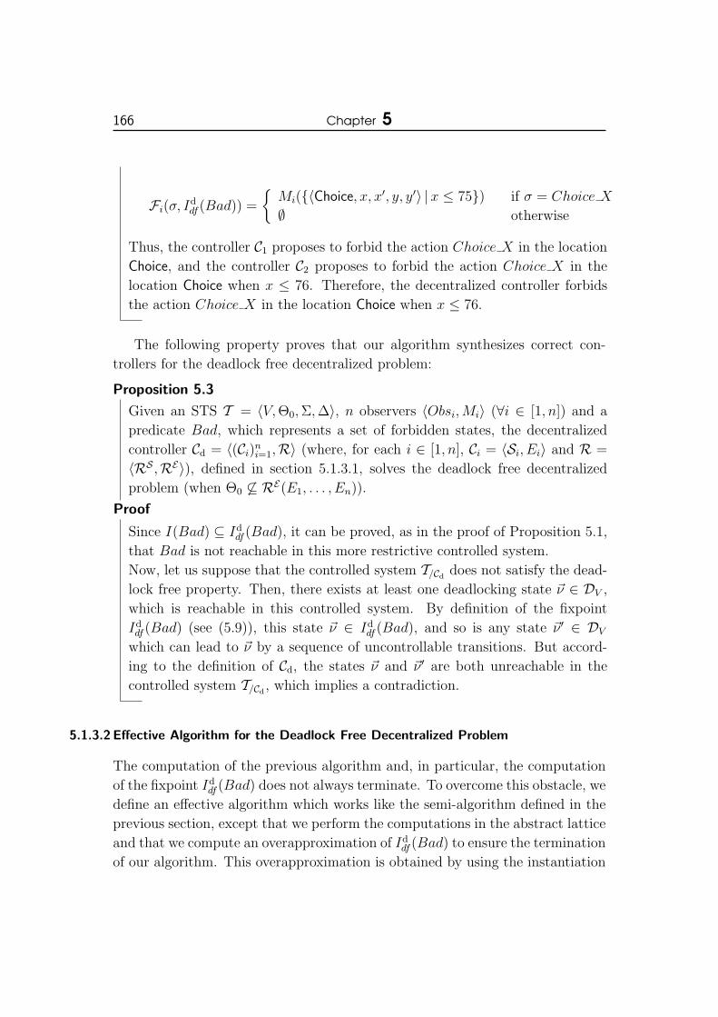
166 Chapter 5
Fi(σ, Iddf (Bad)) =
{Mi({〈Choice, x, x′, y, y′〉 |x ≤ 75}) if σ = Choice X
∅ otherwise
Thus, the controller C1 proposes to forbid the action Choice X in the location
Choice, and the controller C2 proposes to forbid the action Choice X in the
location Choice when x ≤ 76. Therefore, the decentralized controller forbids
the action Choice X in the location Choice when x ≤ 76.
The following property proves that our algorithm synthesizes correct con-
trollers for the deadlock free decentralized problem:
Proposition 5.3
Given an STS T = 〈V,Θ0,Σ,∆〉, n observers 〈Obsi,Mi〉 (∀i ∈ [1, n]) and a
predicate Bad, which represents a set of forbidden states, the decentralized
controller Cd = 〈(Ci)ni=1,R〉 (where, for each i ∈ [1, n], Ci = 〈Si, Ei〉 and R =
〈RS ,RE〉), defined in section 5.1.3.1, solves the deadlock free decentralized
problem (when Θ0 6⊆ RE(E1, . . . , En)).
Proof
Since I(Bad) ⊆ Iddf (Bad), it can be proved, as in the proof of Proposition 5.1,
that Bad is not reachable in this more restrictive controlled system.
Now, let us suppose that the controlled system T/Cddoes not satisfy the dead-
lock free property. Then, there exists at least one deadlocking state ~ν ∈ DV ,
which is reachable in this controlled system. By definition of the fixpoint
Iddf (Bad) (see (5.9)), this state ~ν ∈ Id
df (Bad), and so is any state ~ν ′ ∈ DV
which can lead to ~ν by a sequence of uncontrollable transitions. But accord-
ing to the definition of Cd, the states ~ν and ~ν ′ are both unreachable in the
controlled system T/Cd, which implies a contradiction.
5.1.3.2 Effective Algorithm for the Deadlock Free Decentralized Problem
The computation of the previous algorithm and, in particular, the computation
of the fixpoint Iddf (Bad) does not always terminate. To overcome this obstacle, we
define an effective algorithm which works like the semi-algorithm defined in the
previous section, except that we perform the computations in the abstract lattice
and that we compute an overapproximation of Iddf (Bad) to ensure the termination
of our algorithm. This overapproximation is obtained by using the instantiation
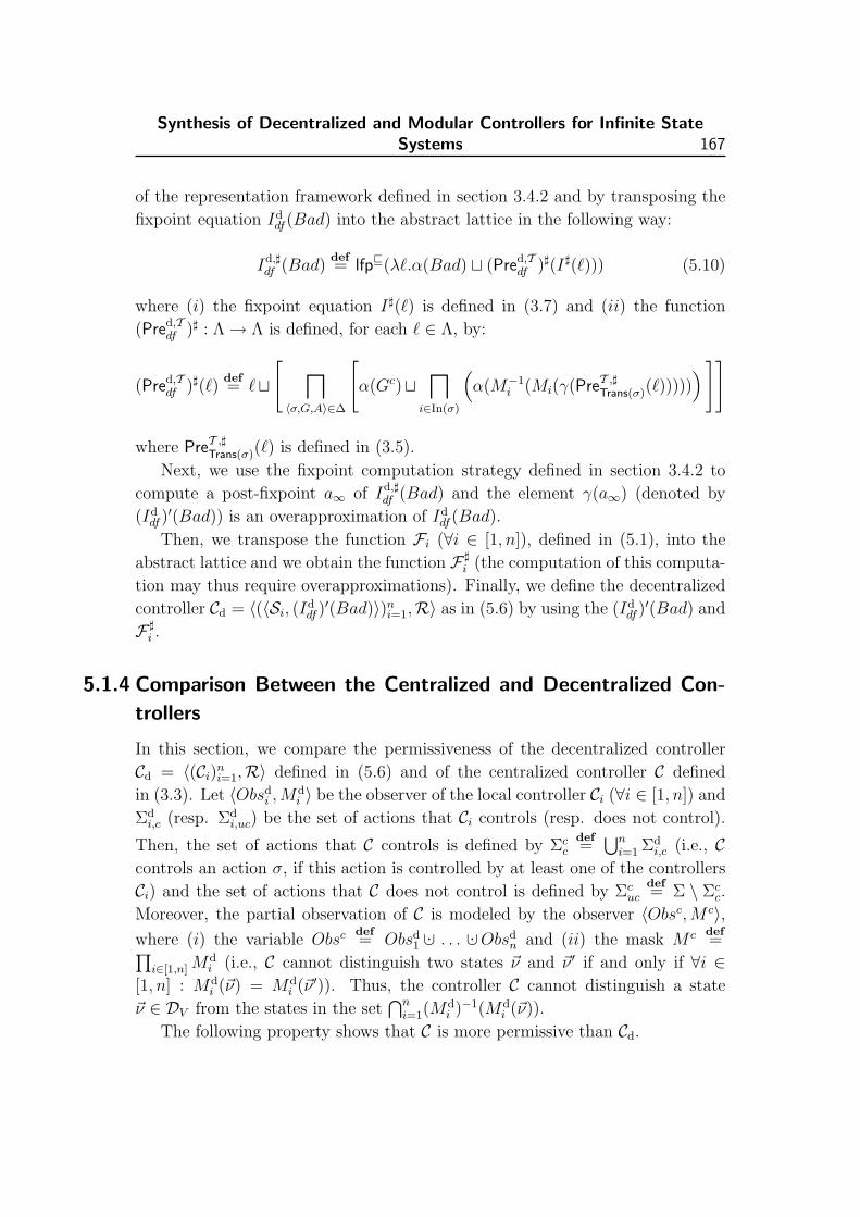
Synthesis of Decentralized and Modular Controllers for Infinite StateSystems 167
of the representation framework defined in section 3.4.2 and by transposing the
fixpoint equation Iddf (Bad) into the abstract lattice in the following way:
Id,]df (Bad)
def= lfpv(λ`.α(Bad) t (Pred,T
df )](I](`))) (5.10)
where (i) the fixpoint equation I](`) is defined in (3.7) and (ii) the function
(Pred,Tdf )] : Λ→ Λ is defined, for each ` ∈ Λ, by:
(Pred,Tdf )](`)
def= `t
[l
〈σ,G,A〉∈∆
[α(Gc)t
l
i∈In(σ)
(α(M−1
i (Mi(γ(PreT ,]Trans(σ)(`)))))
)]]
where PreT ,]Trans(σ)(`) is defined in (3.5).
Next, we use the fixpoint computation strategy defined in section 3.4.2 to
compute a post-fixpoint a∞ of Id,]df (Bad) and the element γ(a∞) (denoted by
(Iddf )
′(Bad)) is an overapproximation of Iddf (Bad).
Then, we transpose the function Fi (∀i ∈ [1, n]), defined in (5.1), into the
abstract lattice and we obtain the function F ]i (the computation of this computa-
tion may thus require overapproximations). Finally, we define the decentralized
controller Cd = 〈(〈Si, (Iddf )
′(Bad)〉)ni=1,R〉 as in (5.6) by using the (Id
df )′(Bad) and
F ]i .
5.1.4 Comparison Between the Centralized and Decentralized Con-
trollers
In this section, we compare the permissiveness of the decentralized controller
Cd = 〈(Ci)ni=1,R〉 defined in (5.6) and of the centralized controller C defined
in (3.3). Let 〈Obsdi ,M
di 〉 be the observer of the local controller Ci (∀i ∈ [1, n]) and
Σdi,c (resp. Σd
i,uc) be the set of actions that Ci controls (resp. does not control).
Then, the set of actions that C controls is defined by Σcc
def=⋃n
i=1 Σdi,c (i.e., C
controls an action σ, if this action is controlled by at least one of the controllers
Ci) and the set of actions that C does not control is defined by Σcuc
def= Σ \ Σc
c.
Moreover, the partial observation of C is modeled by the observer 〈Obsc,M c〉,where (i) the variable Obsc def
= Obsd1 ·∪ . . . ·∪Obsd
n and (ii) the mask M c def=∏
i∈[1,n]Mdi (i.e., C cannot distinguish two states ~ν and ~ν ′ if and only if ∀i ∈
[1, n] : Mdi (~ν) = Md
i (~ν ′)). Thus, the controller C cannot distinguish a state
~ν ∈ DV from the states in the set⋂n
i=1(Mdi )−1(Md
i (~ν)).
The following property shows that C is more permissive than Cd.

168 Chapter 5
x1
x2
x3
x4
x5
x6
Figure 5.2 - Comparison between centralized and decentralized controllers.
Proposition 5.4
Given an STS T = 〈V,Θ0,Σ,∆〉, n observers 〈Obsdi ,M
di 〉 (∀i ∈ [1, n]), an
observer 〈Obsc,M c〉 (where (i) Obsc = Obsd1 ·∪ . . . ·∪Obsd
n and (ii) M c =∏i∈[1,n]M
di ), n partitions Σd
i,c ] Σdi,uc of Σ (∀i ∈ [1, n]), a partition Σc
c ] Σcuc
of Σ (where Σcc =
⋃ni=1 Σd
i,c and Σcuc = Σ \ Σc
c), and a set Bad, which repre-
sents a set of forbidden states, the centralized controller C defined in (3.3) for
the basic problem with the observer 〈Obsc,M c〉 and the partition Σcc ] Σc
uc is
more permissive than the decentralized controller Cd defined in (5.6) for the
basic decentralized problem with the observers 〈Obsdi ,M
di 〉 and the partitions
Σdi,c ] Σd
i,uc (∀i ∈ [1, n]).
Proof
First, we can note that the sets I(Bad) computed for the centralized and
decentralized cases have the same value.
Next, we show that the centralized controller is as permissive as the decen-
tralized controller by proving that ∀~ν ∈ DV ,∀σ ∈ Σcc : σ ∈ S(M c(~ν)) ⇒ σ ∈
RS(S1(Md1 (~ν)), . . . ,Sn(Md
n(~ν))). We suppose that σ ∈ S(M c(~ν)). Then, there
exists a state ~ν ′ 6∈ I(Bad), which is undistinguishable from ~ν and from which
a transition labeled by σ leads to I(Bad). By definition of the mask M c, ~ν ′
belongs to⋂n
i=1(Mdi )−1(Md
i (~ν)), which implies that each local controller Ci(∀i ∈ [1, n]), which controls σ, proposes to forbid this action in the observa-
tion Mdi (~ν) (because ~ν ′ ∈ (Md
i )−1(Mdi (~ν))). Consequently, by definition of the
fusion rule R, we have that σ ∈ RS(S1(Md1 (~ν)), . . . ,Sn(Md
n(~ν))).

Synthesis of Decentralized and Modular Controllers for Infinite StateSystems 169
Finally, the system depicted in Figure 5.2 shows that the centralized controller
C can be strictly more permissive than the decentralized controller Cd. In this
system, (i) the set of states X = {xi | i ∈ [1, 6]}, (ii) the set of initial states
X0 = {x1, x2, x3}, (iii) the set Σ = {σ} (this action can be controlled by all
controllers considered in this example). The set of forbidden states Bad is
equal to {x4, x6}. The decentralized controller is composed of two controllers
C1 and C2: the first one does not distinguish x1 and x2, and the second one does
not distinguish x2 and x3. By definition of the observer of C, this controller
distinguishes all states.
The decentralized controller Cd forbids the action σ in the states x1, x2 and
x3, whereas the centralized controller C only forbids σ in the states x1 and x3,
which implies that C is strictly more permissive than Cd.
A similar property can be obtained for the deadlock free case.
The following proposition gives a sufficient condition which ensures that the
centralized and decentralized controllers have the same permissiveness. This
condition is based on the concept of n-observability defined in [TKU94] and it
intuitively means that if a controllable action is not forbidden by the centralized
controller, then one of the local controllers Ci of the decentralized controller
proposes not to forbid it.
Proposition 5.5
Given an STS T = 〈V,Θ0,Σ,∆〉, n observers 〈Obsdi ,M
di 〉 (∀i ∈ [1, n]), an
observer 〈Obsc,M c〉 (where (i) Obsc = Obsd1 ·∪ . . . ·∪Obsd
n and (ii) M c =∏i∈[1,n]M
di ), n partitions Σd
i,c ] Σdi,uc of Σ (∀i ∈ [1, n]), a partition Σc
c ] Σcuc
of Σ (where Σcc =
⋃ni=1 Σd
i,c and Σcuc = Σ \ Σc
c), and a set Bad, which
represents a set of forbidden states, the centralized controller, C defined
in (3.3) for the basic problem with the observer 〈Obsc,M c〉 and the parti-
tion Σcc ] Σc
uc, and the decentralized controller Cd, defined in (5.6) for the
basic decentralized problem with the observers 〈Obsdi ,M
di 〉 and the partitions
Σdi,c ] Σd
i,uc (∀i ∈ [1, n]), have the same permissiveness if ∀~ν 6∈ I(Bad),∀σ ∈Σc
c : [PostTσ ((M c)−1(M c(~ν)) \ I(Bad)) ∩ I(Bad) = ∅] ⇒ [∃i ∈ In(σ) :
PostTσ ((Mdi )−1(Md
i (~ν)) \ I(Bad)) ∩ I(Bad) = ∅].Proof
In this proof, we use the term equivalence condition to denote the above condi-
tion. By Proposition 5.4, we must only prove that the decentralized controller

170 Chapter 5
is as permissiveness as the centralized controller. For that, we show that if the
centralized controller allows an action σ (∀σ ∈ Σ) in a state ~ν (∀~ν 6∈ I(Bad)),then this action is also allowed by the decentralized controller in the state ~ν.
Two cases must be considered:
• σ ∈ Σcuc: no local controller Ci (∀i ∈ [1, n]) controls σ and hence the
decentralized controller allows the action σ in the state ~ν.
• σ ∈ Σcc : by (3.2) and (3.4), an action σ′ is forbidden by the centralized
controller C in the state ~ν if and only if there exists a state ~ν ′ 6∈ I(Bad)such that (i) M c(~ν) = M c(~ν ′) and (ii) I(Bad) is reachable from ~ν ′ by
a transition labeled by σ′. Therefore, since C allows σ in the state ~ν,
we have that PostTσ ((M c)−1(M c(~ν)) \ I(Bad)) ∩ I(Bad) = ∅. By the
equivalence condition, at least one local controller Ci, which controls σ,
knows that I(Bad) is not reachable from (Mdi )−1(Md
i (~ν)) \ I(Bad) by
a transition labeled by σ. Consequently, by (5.1) and (5.2), Ci proposes
to allow σ in the state ~ν, which implies that the fusion rule allows this
action σ in the state ~ν.
Note that a similar property can be defined for the deadlock free case.
5.2 Synthesis of Modular Controllers
The decentralized framework, that we introduced in the previous section, does
not take into account the fact that, in many applications, systems are often
modeled by several components acting concurrently. This entails that the com-
putation of the decentralized controller is performed on the whole system. In this
section, we will show how, in some cases, the concurrent structure of the system
can be exploited to locally perform the computation of a solution by avoiding
the computation of the global system. To illustrate this point, let us consider the
system T depicted in Figure 3.1. This system has actually the same behavior
as the parallel composition of the subsystems T1 and T2 depicted in Figure 5.3,
and the corresponding controlled system could have been obtained by performing
only local computations on each of these subsystems. As in the previous section,
we focus on the state avoidance control problem, but now we assume that the
system is given by a collection of subsystems acting concurrently. A solution
to this control problem, exploiting the modularity of the system, has already
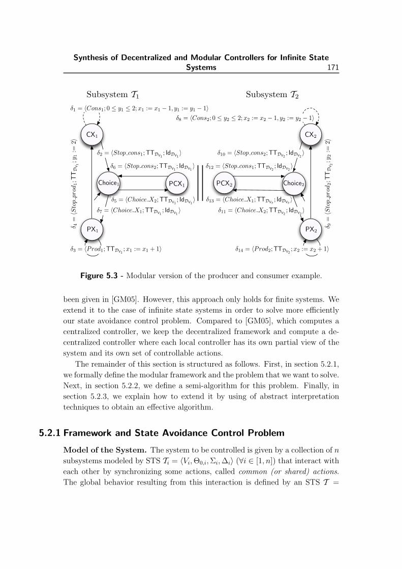
Synthesis of Decentralized and Modular Controllers for Infinite StateSystems 171
δ 4=〈S
top
prod
1;T
TD
V1;y
1:=
2〉
δ2 = 〈Stop cons1;TTDV1; IdDV1
〉
δ6 = 〈Stop cons2;TTDV1; IdDV1
〉
δ3 = 〈Prod1;TTDV1;x1 := x1 + 1〉
δ1 = 〈Cons1; 0 ≤ y1 ≤ 2;x1 := x1 − 1, y1 := y1 − 1〉
δ7 = 〈Choice X1;TTDV1; IdDV1
〉δ5 = 〈Choice X2;TTDV1
; IdDV1〉
CX1
PCX1Choice1
Subsystem T1
Choice2
CX2
PX2
PCX2
Subsystem T2
δ10 = 〈Stop cons2;TTDV2; IdDV2
〉
δ11 = 〈Choice X2;TTDV2; IdDV2
〉
δ12 = 〈Stop cons1;TTDV2; IdDV2
〉
δ8 = 〈Cons2; 0 ≤ y2 ≤ 2;x2 := x2 − 1, y2 := y2 − 1〉
δ14 = 〈Prod2;TTDV2;x2 := x2 + 1〉
δ13 = 〈Choice X1;TTDV2; IdDV2
〉
δ 9=〈S
top
prod
2;T
TD
V2;y
2:=
2〉
PX1
Figure 5.3 - Modular version of the producer and consumer example.
been given in [GM05]. However, this approach only holds for finite systems. We
extend it to the case of infinite state systems in order to solve more efficiently
our state avoidance control problem. Compared to [GM05], which computes a
centralized controller, we keep the decentralized framework and compute a de-
centralized controller where each local controller has its own partial view of the
system and its own set of controllable actions.
The remainder of this section is structured as follows. First, in section 5.2.1,
we formally define the modular framework and the problem that we want to solve.
Next, in section 5.2.2, we define a semi-algorithm for this problem. Finally, in
section 5.2.3, we explain how to extend it by using of abstract interpretation
techniques to obtain an effective algorithm.
5.2.1 Framework and State Avoidance Control Problem
Model of the System. The system to be controlled is given by a collection of n
subsystems modeled by STS Ti = 〈Vi,Θ0,i,Σi,∆i〉 (∀i ∈ [1, n]) that interact with
each other by synchronizing some actions, called common (or shared) actions.
The global behavior resulting from this interaction is defined by an STS T =

172 Chapter 5
〈V,Θ0,Σ,∆〉 obtained by composing the STS Ti with the parallel composition
operator. This operation gives the concurrent behavior of these STS with a
synchronization on the common actions. The parallel composition of two STS is
defined as follows:
Definition 5.6 (Parallel Composition of STS)
Let T1 = 〈V1,Θ0,1,Σ1,∆1〉 and T2 = 〈V2,Θ0,2,Σ2,∆2〉 be two STS such that
V1 ∩ V2 = ∅. The set Σs of shared actions is defined by Σsdef= Σ1 ∩ Σ2.
The parallel composition of T1 and T2, denoted by T1||T2, is given by the
STS T = 〈V,Θ0,Σ,∆〉 where (i) Vdef= V1 ·∪V2, (ii) Θ0
def= Θ0,1 × Θ0,2, (iii)
Σdef= Σ1 ∪ Σ2, and (iv) ∆ is defined as follows for each σ ∈ Σ :
• if σ ∈ Σ1 \ Σs, then, for each transition δ1 = 〈σ,G1, A1〉 ∈ ∆1, we
define a new transition δ = 〈σ,G1, A〉def∈ ∆ where the update function
A : DV1 ×DV2 → DV1 ×DV2 is defined, for each ~ν1 ∈ DV1 and ~ν2 ∈ DV2 ,
by A(〈~ν1, ~ν2〉)def= 〈A1(~ν1), ~ν2〉.
• if σ ∈ Σ2 \ Σs, then, for each transition δ2 = 〈σ,G2, A2〉 ∈ ∆2, we
define a new transition δ = 〈σ,G2, A〉def∈ ∆ where the update function
A : DV1 ×DV2 → DV1 ×DV2 is defined, for each ~ν1 ∈ DV1 and ~ν2 ∈ DV2 ,
by A(〈~ν1, ~ν2〉)def= 〈~ν1, A2(~ν2)〉.
• if σ ∈ Σs, then, for each δ1 = 〈σ,G1, A1〉 ∈ ∆1 and δ2 = 〈σ,G2, A2〉 ∈ ∆2,
we define a new transition δ = 〈σ,G1 ∩ G2, A〉def∈ ∆ where the update
function A : DV1 × DV2 → DV1 × DV2 is defined, for each ~ν1 ∈ DV1 and
~ν2 ∈ DV2 , by A(〈~ν1, ~ν2〉)def= 〈A1(~ν1), A2(~ν2)〉.
Given an STS T = T1|| . . . ||Tn (where T = 〈V,Θ0,Σ,∆〉 and
Ti = 〈Vi,Θ0,i,Σi,∆i〉, for each i ∈ [1, n]), a state ~ν ∈ DV of T is thus
given by an n-tuple 〈~ν1, . . . , ~νn〉 ∈ DV1 × . . . × DVn (where each ~νi ∈ DVigives
the value of the variables of the system Ti). The variables of the subsystems
Ti are not shared, which means that, for each δi = 〈σi, Gi, Ai〉 ∈ ∆i, the guard
Gi and the assignment Ai of δi only use variables of the module Ti; in fact,
the synchronization between the subsystems is achieved through the set Σs of
shared actions where Σsdef=⋃
i6=j∈[1,n](Σi ∩ Σj). In the sequel, we call product
set a product∏n
i=1Bi of local sets Bi ⊆ DVi.

Synthesis of Decentralized and Modular Controllers for Infinite StateSystems 173
Means of Control. The alphabet Σi of each subsystem Ti (∀i ∈ [1, n]) is
partitioned into the set Σi,c of controllable actions and the Σi,uc of uncontrollable
actions i.e., Σi = Σi,uc ] Σi,c. We also assume that the shared actions can
be controlled by all controllers Ci that share them, namely Σs ∩ Σi,uc = ∅.This assumption allows us to fully exploit the structure of the system to be
controlled by performing all computations locally (i.e., on each subsystem). The
set Σc of actions, that can be controlled by at least one controller, is defined by
Σcdef=⋃n
i=1 Σi,c and the set Σi,uc of actions, that cannot be controlled, is defined
by Σucdef= Σ \ Σc =
⋃ni=1 Σi,uc (indeed, with the above assumptions, we have
that Σ \ Σc =⋃n
i=1 Σi,uc). That also induces a partition of the set of transitions
∆ into the set ∆c (resp. ∆i,c) and the set ∆uc (resp. ∆i,uc) in the following way:
〈σ,G,A〉def∈ ∆c (resp. ∆i,c) if σ ∈ Σc (resp. Σi,c), and 〈σ,G,A〉
def∈ ∆uc (resp.
∆i,uc) if σ ∈ Σuc (resp. Σi,uc).
Means of Observation. In the decentralized framework, each local controller
has a partial view of the global system. Here, we assume that there is one
controller per module. We thus consider a special case of partial observation
where each local controller Ci has only a local view of the module, that it controls,
and a perfect observation of all local variables of this subsystem (partial local
observation could be considered, but gives an even more elaborate solution).
Therefore, we associate the following observer with each local controller Ci:
〈Obsi,Mi〉 (5.11)
where (i) Obsidef= Vi, and (ii) the mask Mi : DV → DVi
is defined, for each
state 〈~ν1, . . . , ~νi, . . . , ~νn〉 ∈ DV , by Mi(〈~ν1, . . . , ~νi, . . . , ~νn〉)def= ~νi. In fact,
here we have not a partial observation, but a shared observation, where each
state ~ν = 〈~ν1, . . . , ~νi, . . . , ~νn〉 ∈ DV is equal to the tuple of its observations
〈M1(~ν), . . . ,Mn(~ν)〉.
Definition of the State Avoidance Modular Control Problem. Again, we
want to solve a state avoidance control problem, but a modular one. Therefore,
knowing the modular structure of the system, we assume that the set Bad of
forbidden states is decomposed according to this structure. This set is thus
defined by a finite union of product sets:
Baddef=
m⋃j=1
(n∏
i=1
Bji
)(5.12)

174 Chapter 5
where Bji ⊆ DVi
. Bad can therefore be seen as a disjunction of conjunctions of
local predicates (i.e., of forbidden local states). This definition of Bad does not
cover all possible subsets of states of the system, but it covers a lot of practical
cases that one could want to handle.
Our aim is to synthesize a decentralized controller for the basic decentralized
problem with the additional assumption that we know the structure of the sys-
tem, and we want to exploit this knowledge to perform most of the computations
locally. To avoid confusions, this problem is called basic modular problem and the
decentralized controller, that we want to compute, is called modular controller.
Problem 5.3 (Basic Modular Problem)
Given n STS Ti = 〈Vi,Θ0,i,Σi,∆i〉 (∀i ∈ [1, n]), n observers 〈Obsi,Mi〉(∀i ∈ [1, n]) (defined as in (5.11)), an STS T = 〈V,Θ0,Σ,∆〉 = T1|| . . . ||Tn,
and a set of states Bad (defined as in (5.12)), the basic modular problem
consists in computing a modular controller CM = 〈(Ci)ni=1,R〉 such that (i)
ReachableT/CM∆/CM
((Θ0)/CM) 6= ∅, and (ii) Reachable
T/CM∆/CM
((Θ0)/CM) ∩Bad = ∅.
Note that to fit the modular structure of the system the fusion rule R will be
different from the one defined in (5.3).
5.2.2 Semi-Algorithm for the Basic Modular Problem
Our algorithm, which computes modular controllers for the basic modular prob-
lem, is composed of two parts:
• we compute, using a fixpoint equation, the set I(Bad) of states leading un-
controllably to Bad.
• we compute the modular controller CM. Each local controller of CM forbids,
for each observation, the controllable actions that lead to I(Bad) from a state
compatible with this observation.
Within the modular framework, we want to find a way to compute the set I(Bad)
and the modular controller without having to compute the whole system. We de-
tail these two steps below, but before that, we present some properties regarding
the backward and coreachability operators.
Local Computation of the Backward and Coreachability Operators.
The fixpoint equation defining the set I(Bad) (see (3.1)) is based on the function
Pre and we present a property which allows us to locally compute this function
(see [GM05]).

Synthesis of Decentralized and Modular Controllers for Infinite StateSystems 175
Proposition 5.6 ([GM05])
Given n STS Ti = 〈Vi,Θ0,i,Σi,∆i〉 (∀i ∈ [1, n]), an STS T = 〈V,Θ0,Σ,∆〉 =
T1|| . . . ||Tn, and a set of states B1 × . . .× Bn (where, for each i ∈ [1, n], Bi ⊆DVi
), we have that:
PreTA(B1 × . . .×Bn) =⋃σ∈A
CpreT1σ (B1)× . . .× CpreTn
σ (Bn) (5.13)
where, for each i ∈ [1, n]:
CpreTiσ (Bi) =
{PreTi
σ (Bi) if σ ∈ Σi
Bi otherwise(5.14)
The distributivity of the function PreTA is a direct consequence of the assumptions
that we made on the parallel composition of the subsystems (there is no shared
state variable). This property means that the PreTA operator on the product set
B1 × . . .×Bn can locally be computed on each set Bi.
By using this result, one can locally compute the set CoreachTA(B1× . . .×Bn),
thanks to the following proposition:
Proposition 5.7 ([GM05])
Given n STS Ti = 〈Vi,Θ0,i,Σi,∆i〉 (∀i ∈ [1, n]), an STS T = 〈V,Θ0,Σ,∆〉 =
T1|| . . . ||Tn, a set of states B1 × . . .×Bn (where, for each i ∈ [1, n], Bi ⊆ DVi),
and a set of actions A ⊆ Σ \ Σs, we have that:
CoreachTA(B1×. . .×Bn) = CoreachT1A∩Σ1
(B1)×. . .×CoreachTnA∩Σn
(Bn) (5.15)
Local Computation of the set I(Bad). The following proposition allows us
to locally compute the set I(Bad) of states leading uncontrollably to Bad:
Proposition 5.8 ([GM05])
Given n STS Ti = 〈Vi,Θ0,i,Σi,∆i〉 (∀i ∈ [1, n]), an STS T = 〈V,Θ0,Σ,∆〉 =
T1|| . . . ||Tn with the assumptions defined in section 5.2.1, a set of states⋃mj=1B
j1×. . .×Bj
n (where, for each j ∈ [1,m] and for each i ∈ [1, n], Bji ⊆ DVi
),
we have that:
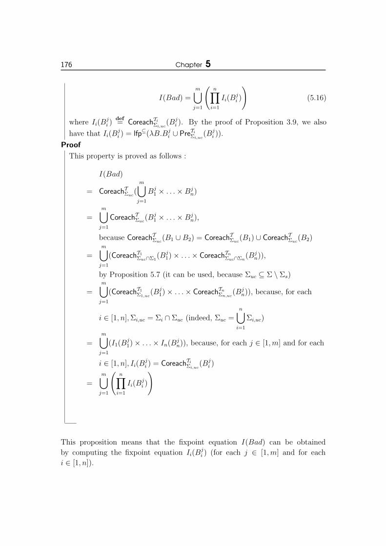
176 Chapter 5
I(Bad) =m⋃
j=1
(n∏
i=1
Ii(Bji )
)(5.16)
where Ii(Bji )
def= CoreachTi
Σi,uc(Bj
i ). By the proof of Proposition 3.9, we also
have that Ii(Bji ) = lfp⊆(λB.Bj
i ∪ PreTiΣi,uc
(Bji )).
Proof
This property is proved as follows :
I(Bad)
= CoreachTΣuc(
m⋃j=1
Bj1 × . . .×Bj
n)
=m⋃
j=1
CoreachTΣuc(Bj
1 × . . .×Bjn),
because CoreachTΣuc(B1 ∪B2) = CoreachTΣuc
(B1) ∪ CoreachTΣuc(B2)
=m⋃
j=1
(CoreachT1Σuc∩Σ1
(Bj1)× . . .× CoreachTn
Σuc∩Σn(Bj
n)),
by Proposition 5.7 (it can be used, because Σuc ⊆ Σ \ Σs)
=m⋃
j=1
(CoreachT1Σ1,uc
(Bj1)× . . .× CoreachTn
Σn,uc(Bj
n)), because, for each
i ∈ [1, n],Σi,uc = Σi ∩ Σuc (indeed, Σuc =n⋃
i=1
Σi,uc)
=m⋃
j=1
(I1(Bj1)× . . .× In(Bj
n)), because, for each j ∈ [1,m] and for each
i ∈ [1, n], Ii(Bji ) = CoreachTi
Σi,uc(Bj
i )
=m⋃
j=1
(n∏
i=1
Ii(Bji )
)
This proposition means that the fixpoint equation I(Bad) can be obtained
by computing the fixpoint equation Ii(Bji ) (for each j ∈ [1,m] and for each
i ∈ [1, n]).

Synthesis of Decentralized and Modular Controllers for Infinite StateSystems 177
Local Computation of the Modular Controller CM = 〈(Ci)ni=1,R〉. We
recall that each local controller Ci (∀i ∈ [1, n]) is only able to observe the variables
Vi of the subsystem Ti. Following the construction of the local controllers Cidefined in subsections 5.1.2.1 and 5.1.3.1 for the decentralized case, we first
investigate how the function Fi, defined in (5.7), can locally be computed2. For
a set of states B =⋃m
j=1Bj (where Bj = Bj
1 × . . . × Bjn is a product set), the
following proposition explains how to locally compute (i.e., on Ti) the function
Fi for each product set Bj of B:
Proposition 5.9
Given n STS Ti = 〈Vi,Θ0,i,Σi,∆i〉 (∀i ∈ [1, n]), an STS T = 〈V,Θ0,Σ,∆〉 =
T1|| . . . ||Tn with the assumptions defined in section 5.2.1, a set of states Bj =
Bj1 × . . .×Bj
n (where, for each i ∈ [1, n], Bji ⊆ DVi
), and an action σ ∈ Σi, we
have that:
Fi(σ,Bj) =
{PreTi
σ (Bji ) if σ ∈ Σi,c
∅ otherwise(5.17)
Proof
If σ 6∈ Σi,c, then Fi(σ,Bj) = ∅ by (5.7). If σ ∈ Σi,c, then:
Fi(σ,Bj) = Mi(PreTσ (Bj)), by (5.7)
= Mi
(CpreT1
σ (Bj1)× . . .× CpreTi
σ (Bji )× . . .× CpreTn
σ (Bjn)),
by Proposition 5.6
= CpreTiσ (Bj
i ), by definition of Mi
= PreTiσ (Bj
i ), by (5.14) (because σ ∈ Σi)
We now explain how each local controller Ci = 〈Si, Ei〉 of the modular controller
CM is computed. According to Proposition 5.8, we write I(Bad) =⋃m
j=1 Ij where
Ij = Ij1 × · · · × Ij
n. To define Si and Ei, we take into account the decomposition
of the system into subsystems and the decomposition of I(Bad) into a union
of product sets. This leads us to a new characterization of these two elements.
Indeed, let us consider the product set Ij = Ij1×· · ·×Ij
n of I(Bad), a controllable
2We recall that Fi(σ,B) gives the set of observations for which Ci proposes to forbid σ
in order to prevent the system from reaching B. We use Fi instead of Fi, because the firstfunction can locally be computed unlike the second one.

178 Chapter 5
action σ ∈ Σc should be disabled in a state ~ν = 〈~ν1, . . . , ~νn〉 due to this product
set whenever:
1. ∀i ∈ [1, n] such that σ ∈ Σi : PostTiσ (~νi) ∈ Ij
i , and
2. ∀i ∈ [1, n] such that σ 6∈ Σi : ~νi ∈ Iji .
i.e., each subsystem, which has σ in its alphabet, can reach a forbidden state
from ~νi by firing a transition labeled by σ and each subsystem, which has not
σ in its alphabet, is already in a forbidden state. Thus, whenever σ 6∈ Σi, the
supervisory function Si (∀i ∈ [1, n]) should indicate whether ~νi ∈ Iji in order to
determine the global control to be applied to the system. In consequence, we
formally define the local controller Ci (∀i ∈ [1, n]) as follows:
Cidef= 〈Si, Ei〉 (5.18)
where the elements Si and Ei are defined in the following way:
• For each state ~ν = 〈~ν1, . . . , ~νi, . . . , ~νn〉 ∈ DV , the supervisory function Si only
observes ~νi ∈ DObsiand is given by the pair Si(~νi)
def= 〈P i(~νi),Bi(~νi)〉 where:
• the function P i(~νi) gives the set of pairs 〈j, σ〉 such that Ci proposes to
forbid the action σ in the state ~νi because of the product set Ij; compared
to the decentralized approach, we memorize the index of the product set
for which σ must be forbidden in the state ~νi:
P i(~νi)def= {〈j, σ〉 | (σ ∈ Σi,c) ∧ (j ∈ [1,m]) ∧ (~νi ∈ Fi(σ, I
j))} (5.19)
• the function Bi(~νi) gives the set of indices j such that ~νi belongs to the
forbidden set Iji :
Bi(~νi)def= {j | (j ∈ [1,m]) ∧ (~νi ∈ Ij
i )} (5.20)
As explained above, this information will be used by the fusion rule to know
whether ~νi ∈ Iji .
• The set Eidef= {〈j, Ej
i 〉 | (j ∈ [1,m]) ∧ (Eji = Ij
i )}.
We also need to redefine the elements RS and RE of the fusion rule R (denoted
by RSM and RE
M hereafter to stress the modular architecture) to take into account
the decomposition of I(Bad) into product sets as well as the new definition of
the supervisory function. The fusion rule R is defined by:
R def= 〈RS
M,REM〉 (5.21)
where, for each ~ν = 〈~ν1, . . . , ~νn〉 ∈ DV , we define:
Synthesis of Decentralized and Modular Controllers for Infinite StateSystems 179
• the fusion rule RSM by:
RSM(S1(~ν1), . . . ,Sn(~νn))
def= {σ ∈ Σc | ∃j ∈ [1,m] : [(∀i ∈ [1, n] such
thatσ ∈ Σi : 〈j, σ〉 ∈ P i(~νi))∧(∀i ∈ [1, n] such that σ 6∈ Σi : j ∈ Bi(~νi))]}
(5.22)
Thus, as explained above, a controllable action σ is forbidden in the state ~ν if
there exists a product set Ij = Ij1 × . . .× Ij
n such that (i) each subsystem Ti,
which has σ in its alphabet, can reach Iji from ~νi by firing a transition labeled
by σ, and (ii) each subsystem Ti, which has not σ in its alphabet, is in a state
of Iji .
• the fusion ruleREM as follows: ~ν
def∈ RE
M(E1, . . . , En) if and only if ∃j ∈ [1,m] :
~ν ∈ Ej1 × . . . × Ej
n (where, for each i ∈ [1, n], 〈j, Eji 〉 ∈ Ei). We can remark
that, as expected, REM forbids the states of I(Bad).
Finally, the modular controller CM is defined by the n local controllers Ci given
in (5.18) and by the fusion rule given in (5.21):
CMdef= 〈(Ci)n
i=1,R〉 (5.23)
The set I(Bad) and the control functions Fi are computed offline. Next,
during the execution of the system, when the system arrives in a state ~ν =
〈~ν1, . . . , ~νn〉 ∈ DV , each local controller Ci receives the observation ~νi and com-
putes online the pair Si(~νi) = 〈P i(~νi),Bi(~νi)〉; this computation is based on the
functions Fi. The fusion rule RSM(S1(~ν1), . . . ,Sn(~νn)) is then computed online
from these control decisions and gives the actions that the system cannot execute.
Example 5.3
We compute a modular controller CM = 〈〈C1, C2〉,R〉 for the subsystems T1 and
T2 depicted in Figure 5.3. The system Ti = 〈Vi,Θ0,i,Σi,∆i〉 (for i = 1, 2) has a
tuple Vi = 〈`i, xi, yi〉 of three variables where (i) `i ∈ {Choicei,PXi,CXi,PCXi}gives the current location of Ti, (ii) xi ∈ Z gives the number of parts Xi, and
(iii) yi ∈ Z gives the number of parts Xi that can be produced. The system
Ti does not control the action Consi (i.e., Σi,uc = {Consi}) and its initial
state is 〈Choicei, 0, 0〉. The global system T = T1||T2 = 〈V,Θ0,Σ,∆〉 has thus
a tuple V = 〈〈`1, x1, y1〉, 〈`2, x2, y2〉〉 of six variables. The modular controller
must prevent the system T from reaching the set Bad defined by the product
set B11 × B1
2 where B1i = {〈CXi, xi, yi〉 | (xi ≤ 10) ∧ (yi ∈ [0, 2])} (for i = 1, 2).
The computation of the set I(Bad) = I1(B11)× I2(B1
2) gives (for i = 1, 2):

180 Chapter 5
Ii(B1i ) = B1
i ∪{〈CXi, xi, yi〉 | [(xi ≤ 11)∧(yi ∈ [1, 2])]∨[(xi ≤ 12)∧(yi = 2)]}
Next, the computation of the control function Fi (for i = 1, 2) gives:
Fi(σ, I(Bad)) =
{{〈PXi, xi, yi〉 |xi ≤ 12} if σ = Stop prodi
∅ otherwise
The supervisory function Si = 〈P i,Bi〉 (for i = 1, 2) is then defined as follows:
P i(~νi) =
{{〈1, Stop prodi〉} if ~νi ∈ {〈PXi, xi, yi〉 |xi ≤ 12}∅ otherwise
Bi(~νi) =
{{1} if ~νi ∈ Ii(B1
i )
∅ otherwise
The fusion rule RSM forbids:
• the action Stop prod1 when the subsystem T1 is in a state ~ν1 ∈{〈PX1, x1, y1〉 |x1 ≤ 12} and the subsystem T2 is in a state ~ν2 ∈{〈CX2, x2, y2〉 | [(x2 ≤ 10)∧(y2 ∈ [0, 2])]∨[(x2 ≤ 11)∧(y2 ∈ [1, 2])]∨[(x2 ≤12) ∧ (y2 = 2)]}.
• the action Stop prod2 when the subsystem T1 is in state ~ν1 ∈{〈CX1, x1, y1〉 | [(x1 ≤ 10) ∧ (y1 ∈ [0, 2])] ∨ [(x1 ≤ 11) ∧ (y1 ∈[1, 2])] ∨ [(x1 ≤ 12) ∧ (y1 = 2)]} and the subsystem T2 is in a state
~ν2 ∈ {〈PX2, x2, y2〉 |x2 ≤ 12}.
Proposition 5.10
Given n STS Ti = 〈Vi,Θ0,i,Σi,∆i〉 (∀i ∈ [1, n]), an STS T = 〈V,Θ0,Σ,∆〉 =
T1|| . . . ||Tn with the assumptions defined in section 5.2.1, and a set of states⋃mj=1B
j1×. . .×Bj
n (where, for each j ∈ [1,m] and for each i ∈ [1, n], Bji ⊆ DVi
),
the modular controller CM, defined in (5.23), solves the basic modular problem
(when Θ0 6⊆ REM(E1, . . . , En)).
Proof
We prove by induction on the length ` of the sequences of transitions (these
sequences begin in an initial state) that ReachableT/CM∆/CM
((Θ0)/CM)∩ I(Bad) = ∅.
Since Bad ⊆ I(Bad), this property implies that ReachableT/CM∆/CM
((Θ0)/CM) ∩
Bad = ∅:

Synthesis of Decentralized and Modular Controllers for Infinite StateSystems 181
• Base case (` = 0): the controlled system T/CMstarts its execution in a
state ~ν, which belongs to Θ0 and which is not in REM(E1, . . . , En). Thus,
this state does not belong to I(Bad).
• Induction case: we suppose that the proposition holds for the sequences
of transitions of length less than or equal to ` and we prove that this
property remains true for the sequences of transitions of length ` + 1.
By induction hypothesis, each state ~ν = 〈~ν1, . . . , ~νn〉 reachable by a
sequence of transitions of length ` does not belong to I(Bad) and we
show that each transition δ = 〈σ,G,A〉 ∈ ∆, which can lead to a state
~ν ′ = 〈~ν ′1, . . . , ~ν ′n〉 ∈ I(Bad) from this state ~ν in the system T , cannot be
fired from ~ν in the controlled system T/CM. For that, we consider two
cases; let Ij = Ij1× . . .× Ij
n be a product set of I(Bad) such that ~ν ′ ∈ Ij:
• either δ ∈ ∆uc, then ~ν ∈ I(Bad) (by (3.1)), which is impossible by
hypothesis.
• or δ ∈ ∆c, then we show that this transition is forbidden by the
fusion rule. We can first remark that, for any i ∈ [1, n], if σ ∈ Σi
and if σ ∈ Σc, then σ ∈ Σi,c. Next, we prove the desired property by
reasoning as follows:
• for each i ∈ [1, n] such that σ 6∈ Σi, we have that ~νi = ~ν ′i (by
definition of the parallel composition of STS), which implies that
~νi ∈ Iji , because ~ν ′ ∈ Ij. Therefore, by (5.20), we have that
∀i ∈ [1, n] such that σ 6∈ Σi : j ∈ Bi(~νi).
• for each i ∈ [1, n] such that σ ∈ Σi, we have that ~νi ∈ PreTiσ (~ν ′i) (by
definition of the parallel composition of STS), which implies that
~νi ∈ PreTiσ (Ij
i ), because ~ν ′ ∈ Ij. Therefore, by (5.17), and (5.19)
we have that ∀i ∈ [1, n] such that σ ∈ Σi : 〈j, σ〉 ∈ P i(~νi).
Consequently, by (5.22), we have that σ is forbidden by the fusion
rule RSM in the state ~ν.
As explained in the introduction of this chapter, the advantage of the modular
approach w.r.t. the decentralized approach is that we exploit the structure of the
distributed system to be controlled to efficiently compute controllers. To exploit
this structure, we defined the controller and the fusion rule differently from the
decentralized approach. This implies that the controlled behaviors resulting from

182 Chapter 5
the decentralized and modular controls are not necessarily identical and an open
question consists in comparing the permissiveness of these approaches.
5.2.3 Effective Algorithm for the Basic Modular Problem
The effective computation is here straightforward. We compute, for each i ∈ [1, n]
and for each j ∈ [1,m], an overapproximation I ′i(Bji ) of the fixpoint equation
Ii(Bji ) by using the approach described in section 3.4.2. Next, we transpose
the control function Fi (∀i ∈ [1, n]) into the abstract lattice and we obtain the
abstract function F ]i (the computation of this function may require overapprox-
imations). Finally, we define our modular controller CM as in (5.23) by using
I ′i(Bji ) (∀i ∈ [1, n] and ∀j ∈ [1,m]) and F ]
i (∀i ∈ [1, n]) instead of Ii(Bji ) and Fi.
5.3 Experimental Evaluation
Our algorithms, that synthesize decentralized and modular controllers, have re-
spectively been implemented in our tool SMACS (Symbolic MAsked Controller
Synthesis) and Mod-SMACS (Modular Symbolic MAsked Controller Synthesis).
A detailed description of SMACS is given in appendix A. The tool Mod-SMACS
has a lot of similarities with SMACS and is thus not described.
We define several examples and present the solutions computed by SMACS
or Mod-SMACS for these systems in order to experimentally evaluate our
method. Our experiments are performed with the lattice of convex polyhedra.
Toy Example. We consider the system depicted in Figure 3.14. As a reminder,
this STS has explicit locations ` ∈ {`i | i ∈ [0, 8]} and two integer variables x and
y. A state of the system is a triple 〈`, x, y〉. The actions ci (for i ∈ [0, 3]) are
controllable and the actions ui (for i ∈ [0, 1]) are uncontrollable. The initial state
is 〈`0, 0, 0〉 and the set Bad is defined by {〈`6, k1, k2〉|k1, k2 ∈ Z}. We consider
several cases:
• The local controller C1 has a full observation of the system and the lo-
cal controller C2 does not distinguish the locations `3 and `4 (i.e., ∀x, y ∈Z : M2(〈`3, x, y〉) = M2(〈`4, x, y〉)). We first suppose that the deadlock
free property must not be ensured. SMACS computes a set I(Bad) =
Bad ∪ {〈`2, x, y〉 | 10 ≤ x ≤ 1000}. To prevent the system from reaching
this set, it defines a controller C1 that disables the action c0 in the loca-
tion `3 when (10 ≤ x ≤ 1000) ∧ (y ≥ x) and a controller C2 that disables

Synthesis of Decentralized and Modular Controllers for Infinite StateSystems 183
l8
l0
< #true >
[u1]{y = x,x = y}
l7
< #true >
[u0]{x = ((2. * y) + 4.)}
l6
l5
l3
< #true >
[c2]{y = (x + 2.)}
l4
< #true >
[c0]{x = (4. * x)}
l2
< (x<=y) AND NOT ((((1000. + (-1. * x)) + (0. * y))>=0.) AND
((0. + (-1. * x)) + (1. * y)) >=0.) AND ((-10. + (1. * x)) + (0. * y)) >=0.] > [c0] {}
< #true >
[c3]{y = (y + 2.)}
< x == 10. >
[u0]{}
< x <= 1000. >
[u1]{x = (x - 1.)}
l1
< #true >
[u1]{x = (y - 5.)}
< #true >
[c1]{y = 2.,x = 5.}
< #true >
[c3]{x = (x + 1.)}
< #true >
[c2]{}
Figure 5.4 - Controlled system generated by SMACS for the toy example when
C1 has a full observation of the system, C2 does not distinguish the
locations `3 and `4, and the deadlock free property is not ensured.

184 Chapter 5
the action c0 in the locations `3 and `4 when (10 ≤ x ≤ 1000) ∧ (y ≥ x).
The global control is similar to the control policy of C1. The graphical
output of the controlled system generated by SMACS is depicted in Fig-
ure 5.4. When the deadlock free property must be ensured, SMACS com-
putes a set Idf (Bad) = Bad ∪ {〈`2, x, y〉 |x ≥ 10}. The states in the set
{〈`2, x, y〉 | 10 ≤ x ≤ 1000} are forbidden, because they uncontrollably lead
to Bad and the states in the set {〈`2, x, y〉 |x > 1000} are forbidden, because
they are in deadlock. SMACS defines a controller C1 that forbids the action
c0 in the location `3 when (x ≥ 10) ∧ (y ≥ x) and a controller C2 that forbids
the action c0 in the locations `3 and `4 when (x ≥ 10) ∧ (y ≥ x). Again, the
global control is similar to the control policy of C1.
• The local controller C1 has a full observation of the system and the local
controller C2 does not observe the variable x (i.e., for each ~ν = 〈`, x, y〉 ∈ DV ,
the set of states that C2 does not distinguish from ~ν is given by {〈`2, x′, y〉 |x′ ∈Z}). We first suppose that the deadlock free property must not be ensured.
SMACS computes a set I(Bad) = Bad ∪ {〈`2, x, y〉 | 10 ≤ x ≤ 1000}. Next,
it defines a controller C1 that forbids the action c0 in the location `3 when
(10 ≤ x ≤ 1000)∧ (y ≥ x) and a controller C2 that forbids the action c0 in the
location `3 when y ≥ 10. The global control is similar to the control policy of
C1. When the deadlock free property must be ensured, SMACS computes a
set Idf (Bad) = Bad ∪ {〈`2, x, y〉 |x ≥ 10}. Next, SMACS defines a controller
C1 that forbids the action c0 in the location `3 when (x ≥ 10) ∧ (y ≥ x) and
a controller C2 which forbids the action c0 in the location `3 when (y ≥ 10).
The global control is similar to the control policy of C1.
• The local controller C1 does not distinguish the locations `3 and `4, and the
local controller C2 does not observe the variable x. We first suppose that the
deadlock free property must not be ensured. SMACS computes a set I(Bad) =
Bad∪{〈`2, x, y〉 | 10 ≤ x ≤ 1000}. Next, it defines a controller C1 that forbids
the action c0 in the locations `3 and `4 when (10 ≤ x ≤ 1000) ∧ (y ≥ x)
and a controller C2 that forbids the action c0 in the location `3 when y ≥ 10.
The global control consists in forbidding the action c0 in the location `3 when
(10 ≤ x ≤ 1000)∧(y ≥ x). When the deadlock free property must be ensured,
SMACS computes a set Idf (Bad) = Bad∪{〈`2, x, y〉 |x ≥ 10}. To prevent the
system from reaching this set, SMACS defines a controller C1 that forbids the
action c0 in the locations `3 and `4 when (x ≥ 10)∧(y ≥ x) and a controller C2that forbids the action c0 in the location `3 when (y ≥ 10). The global control

Synthesis of Decentralized and Modular Controllers for Infinite StateSystems 185
System Number Time Maximal
of Variables (seconds) Memory (MB)
Toy 130 9.4 72
example 170 21.1 84
210 35.9 96
250 58.9 108
290 93.3 144
Table 5.1 - Time (in seconds) and memory (in MB) used by SMACS to synthe-
size a decentralized controller (composed of two local controllers) for
modified versions of the toy example.
consists in forbidding the action c0 in the location `3 when (x ≥ 10)∧ (y ≥ x).
All these computations are done in few ms. Next, we consider modified versions
of the toy example where we add variables to make more complex the system to
be controlled. The set of forbidden states is defined over these new variables and
SMACS must compute a local controller C1 (this controller does not distinguish
the locations `3 and `4) and a local controller C2 (this controller does not observe
the variable x) which satisfy this specification. The results are reported in Ta-
ble 5.1. For example, when the system has 170 variables, SMACS computes local
controllers C1 and C2 which fulfill the requirements in 21.1 seconds and uses, for
that, 84 MB of RAM.
Producer and Consumer. We consider a modified version of the producer
and consumer example depicted in Figure 3.1, where the transitions δ1, δ4, δ5and δ8 are respectively replaced by 〈Cons; 0 ≤ y ≤ 500;x := x − 1, y := y − 1〉,〈Stop prod; TTDV
; y := 500〉, 〈Cons′; 0 ≤ y′ ≤ 500;x′ := x′ − 1, y′ := y′ − 1〉,and 〈Stop prod′; TTDV
; y′ := 500〉, which makes the system more complex to be
controlled. The set Bad of forbidden states is defined by {〈CX, x, x′, y, y′〉 | (x ≤10)∧ (y ∈ [0, 500])}∪{〈CX′, x, x′, y, y′〉 | (x′ ≤ 10)∧ (y′ ∈ [0, 500])}. The aim is to
synthesize two local controllers C1 and C2 which satisfy the control specification.
C1 does not control the actions Cons, Cons′ and Stop prod′, and C2 does not
control the actions Cons, Cons′ and Stop prod. We consider several cases:
• The local controller C1 does not observe the variables x and y (i.e., for each
~ν = 〈`, x, x′, y, y′〉 ∈ DV , the set of states that C1 does not distinguish from
~ν is given by {〈`, x1, x′, y1, y
′〉 |x1, y1 ∈ Z}), the local controller C2 has a full
observation of the system, and the deadlock free property is not ensured.

186 Chapter 5
SMACS defines a controller C1 which always forbids the action Stop prod in
the location PX and a controller C2 which forbids the action Stop prod′ in the
location PX′ when x′ ≤ 510. The global control consists in forbidding the
action Stop prod in the location PX and the action Stop prod′ in the location
PX′ when x′ ≤ 510.
• The local controller C1 has a full observation of the system, the controller
local C2 does not observe the variable x′ in the interval [500, 600] (i.e., for each
state ~ν = 〈`, x, x′, y, y′〉 ∈ DV , if x′ 6∈ [500, 600], then C2 perfectly observes this
state, otherwise the set of states that C2 does not distinguish from ~ν is given
by {〈`, x, x′1, y, y′〉 |x′1 ∈ [500, 600]}), and the deadlock free property is not
ensured. SMACS defines a controller C1 which forbids the action Stop prod
in the location PX when x ≤ 510 and a controller C2 which forbids the action
Stop prod′ in the location PX′ when x′ ≤ 600. The global control consists
in forbidding the action Stop prod in the location PX when x ≤ 510 and the
action Stop prod′ in the location PX′ when x′ ≤ 600.
• The local controller C1 does not observe the variables x and y, the local con-
troller C2 does not observe the variables x′ in the interval [500, 600], and the
deadlock free property is not ensured. SMACS defines a controller C1 which
always forbids the action Stop prod in the location PX and a controller C2which forbids the action Stop prod′ in the location PX′ when x′ ≤ 600. The
global control consists in forbidding the action Stop prod in the location PX
and the action Stop prod′ in the location PX′ when x′ ≤ 600.
All these computations are done in few ms. Then, we consider modified versions
of the producer and consumer example. The system is made more complex by
producing n (where n > 0) kinds of parts. The production of each kind of parts
requires the definition of two variables xi and yi. The control requirements consist
in ensuring that there are at least 11 parts of each kind. SMACS must compute n
local controllers Ci (∀i ∈ [1, n]). Each controller Ci does not observe the value of
the variable xi when it belongs to the interval [400, 600]. The results are reported
in Table 5.2. For example, when the system has 80 variables (i.e., there are 40
kinds of parts), SMACS computes a solution which fulfills the requirements in
50.2 seconds and uses, for that, 168 MB of RAM.
Comparison Between the Modular and Decentralized Controllers.
Now, we compare our modular and decentralized controllers. The experiments
have been done on the producer and consumer example and are reported in

Synthesis of Decentralized and Modular Controllers for Infinite StateSystems 187
System Number Time Maximal
of Variables (seconds) Memory (MB)
Producer and consumer 40 4.4 84
example 80 50.2 168
120 231.6 348
140 404.4 456
160 686.9 660
Table 5.2 - Time (in seconds) and memory (in MB) used by SMACS to synthe-
size a decentralized controller (composed of two local controllers) for
modified versions of the producer and consumer example.
Table 5.3. For the decentralized case, we consider the producer and consumer
system described above and producing n kinds of parts Xi (∀i ∈ [1, n]). The
decentralized controller must ensure that there are at least 11 parts of each kind
and is composed of n local controllers Ci. Each local controller Ci can only ob-
serve the variables `, xi and yi involved in the production of the parts of kind
Xi. Note that these masks are different from the ones used in the experiments
reported in Table 5.2. This explains why the time performance is not indentical
in Tables 5.2 and 5.3. For the modular case, the system to be controlled is com-
posed of n subsystems Ti. Each subsystem Ti produces the parts of kind Xi and
the modular controller must ensure that there are at least 11 parts of each kind.
Our experiments show that the performance (time and memory) of the modular
controller is better than the one of the decentralized controller (see Table 5.3)
and that both controllers are always �p-maximal. In this case the controlled be-
haviors resulting from the decentralized and modular approaches are identical.
For example, when 100 kinds of parts must be produced, the modular controller
computes the solution 50 times faster and uses 100 times less memory.

188 Chapter 5
System Number Decentralized Modular
of parts Time Maximal Time Maximal
to be (seconds) Memory (seconds) Memory
produced (MB) (MB)
Producer 20 1.3 84 0.2 < 12
and 30 5 108 0.5 < 12
consumer 40 12.7 168 0.7 < 12
example 50 28 228 1.2 < 12
60 53.5 300 1.5 < 12
70 93.7 444 2.2 < 12
80 153.8 612 3.2 < 12
90 240.8 852 6.2 < 12
100 362.7 1128 7.1 < 12
Table 5.3 - Time (in seconds) and memory (in MB) used by SMACS and Mod-
SMACS to control modified versions of the producer and consumer
example.
Chapter
6Distributed Supervisory Control of
FIFO Systems
In chapter 5, we were interested in the decentralized and modular controls
of infinite state systems. These methods are useful for the control of
distributed systems with synchronous communications. Both methods
assume the existence of a synchronization mechanism (fusion rule) which allows
the decentralized (resp. modular) controller to collect the control decisions of
each local controller and to define the global control policy from these local
decisions.
In this chapter, we consider the control of a more complex class of distributed
systems: the distributed systems with asynchronous communications. These
systems are generally composed of several subsystems that can be located at
different places in such a way that communications between them can no longer
be assumed as instantaneous. In this context, one has to take into account
the duration of the communications and thus the asynchronous nature of the
communication events. The decentralized and modular frameworks cannot then
be used for the control of these systems, since their synchronization mechanism,
which defines the global control policy, is no more valid in this context.
In this chapter, we thus propose a method for the control of distributed
systems with asynchronous communications. In this method the system to
be controlled is composed of n subsystems that asynchronously communicate
190 Chapter 6
through reliable unbounded FIFO channels. These subsystems are modeled
by communicating finite state machines [BZ83a] that explicitly represent the
communications of a distributed system. Each subsystem is controlled by a
local controller. The local controllers can communicate with each other through
reliable unbounded FIFO channels. These communications allow them to
exchange information to refine their knowledge of the global state of the system
and hence their control policy. The state space of the distributed system to be
controlled can be infinite, because the FIFO channels are unbounded. Moreover,
the state avoidance control problem that we want to solve is undecidable and
hence we use abstract interpretation techniques to ensure the termination of the
computations. The used techniques to obtain an effective algorithm are actually
the same as the ones used in chapters 3, 4, and 5, except that we perform the
computations in a different abstract lattice. This lattice is the one of regular
languages, which allows us to abstract the content of FIFO channels by regular
languages.
Related Works. In [Tri02], Tripakis studies the time complexity of some prob-
lems related to the decentralized control with communication. The specification
is given by a set φ of responsiveness properties over an alphabet Σ. A respon-
siveness property is a formula of the form a b (where a, b ∈ Σ) and it is
satisfied by a (finite or infinite) string ` over Σ if an action b eventually occurs
after every action a in `. The problem under consideration consists in deciding if
there exists a decentralized controller Cd such that the maximal language Lmax
of the controlled system T/Cdsatisfies φ. This language Lmax is defined by all
infinite strings of the controlled system and all finite strings that cannot be ex-
tended by an action of Σ (i.e., the system is in a deadlocking state). The author
proves that the problem is undecidable when there is no communication or when
the communication delays are unbounded. He conjectures that the problem is
decidable when the communication delays are bounded. In [XK09], Kumar and
Xu propose a distributed algorithm which computes an estimate of the current
state of a system. More precisely, local sites maintain and update local state
estimates from their local observation of the system and information received
from the other sites. This information is exchanged through reliable unbounded
FIFO channels. The control of distributed systems also received attention in the
domain of Petri nets, but these works generally use a synchronization mechanism
to coordinate the control decisions of the local controllers. In [HB91], Haoxun
and Baosheng define an algorithm for the state avoidance control problem. Their
Distributed Supervisory Control of FIFO Systems 191
method consists in augmenting the system with coordination places, that act as
semaphores and are used by the local controllers to coordinate their control de-
cisions. In [Dar05], Darondeau synthesizes distributed controllers by using Petri
nets during the computations. More precisely, he states a sufficient condition
which allows us to decide if a controller can be implemented by a particular class
of Petri nets; this class is a strict subclass of finite automata. Then, he imposes
a constraint on the produced Petri net, which ensures that it can be translated
into several communicating automata C1, . . . , Cn. These controllers can commu-
nicate through bounded channels, for which no assumption is made regarding the
order and the delay of delivery of the messages. Finally, they are used to control
the distributed system which is also composed of n communicating automata
T1, . . . , Tn.
The remainder of this chapter is structured as follows. In section 6.1, we
present an overview of our control method. Next, in section 6.2, we define the
formalism of communicating finite state machines, that we use to model dis-
tributed systems. In section 6.3, we formally define the control mechanisms and
the state avoidance control problem that we want to solve. Then, in section 6.4,
we provide an algorithm, that allows us to compute an estimate of the current
state of a distributed system. In section 6.5, we define a control algorithm,
based on this state estimate algorithm, for our state avoidance control problem
and we explain how we can ensure the termination of this control algorithm by
using abstract interpretations techniques. Finally, in section 6.6, we prove some
properties presented in section 6.4.
6.1 Overview of the Method
We are interested in the distributed supervisory control of infinite state systems,
consisting of asynchronous networks of subsystems where communication is pos-
sible through reliable unbounded FIFO channels. We associate a local controller
with each subsystem. Each local controller can observe the last action fired by
its subsystem1 and disable some of its actions. Our goal is that the global system
under the control of these local controllers satisfies a global safety property. In
order to achieve a more permissive control, the controllers have a memory and
can asynchronously communicate through the existing FIFO channels.
1A controller observes the actions fired by its subsystem in order to have a better knowledgeabout this system. Note that since we consider, in the sequel, deterministic systems, thecontroller can infer the current location of its subsystem.

192 Chapter 6
In this section, we present, with an example, the communicating finite state
machines, which model the distributed systems to be controlled, as well as the
kind of properties we want to ensure and the main idea of our method.
Introductory Example. We illustrate our method on a faulty communication
protocol (see Figure 6.1 for the structure of the system). In this example, the
subsystem T2 can send two kinds of messages to the subsystem T1: a and b. The
subsystem T1 can receive those messages at any time. However, an error occurs
when the subsystem T1 receives the message a in the location A0. The protocol
depicted in Figure 6.1 tries to avoid this error by using an additional subsystem
T3 and synchronization messages c and d. The subsystem T1 sends the message
c to T2 to start the communications. T1 can then read the messages a and b sent
by T2. When T2 has sent all messages a and b, it sends a message d to T1, which
passes through the subsystem T3. After the reception of this message d, T1 also
sends a message d to T2 to inform it that it has read this message. There are four
FIFO channels: (i) channel 1: T1 → T2, (ii) channel 2: T2 → T1, (iii) channel 3:
T2 → T3, and (iv) channel 4: T3 → T1. The action of sending the message c into
the channel 1 is denoted by 1!c, and the action of receiving the message c from
the channel 1 is denoted by 1?c. However, this protocol does not ensure that
the subsystem T1 does not receive the message a in the location A0. Indeed, a
possible counter-example is given by the following sequence of actions that starts
in the initial location 〈A0, B0, D0〉 with all channels empty:
• The subsystem T1 sends the message c: A01!c→ A1
• The subsystem T2 receives the message c: B01?c→ B1
• The subsystem T2 sends the message a: B12!a→ B2
• The subsystem T2 sends the message d: B23!d→ B3
• The subsystem T3 receives the message d: D03?d→ D1
• The subsystem T3 sends the message d: D14!d→ D0
• The subsystem T1 receives the message d: A14?d→ A2
• The subsystem T1 sends the message d: A21!d→ A0
• The subsystem T1 receives the message a in the location A0: A02?a→ Aerror
We would like to add three controllers C1, C2 and C3 to ensure that the sub-
system T1 cannot receive the message a in the location A0. The controller Ci(∀i ∈ [1, 3]) controls the subsystem Ti.

Distributed Supervisory Control of FIFO Systems 193
A02?a
A1
Aerror
A2
T1
1!c
2?b
2?a
4?d2?a
2?b
1!d
2?b
T2
B0
B1
B2
B3
1?c
2!a 3!d
T3
D0 D1
4!d
3?d T1 T2
T3
CommunicationArchitecture
1
234
2!b
1?d
3!d
Figure 6.1 - Introductory example
194 Chapter 6
Control Problem. We want to disable some actions to ensure that this error
state cannot be reached. We assume that inputs are uncontrollable and outputs
are controllable (i.e., they may be disabled by the local controllers). Thus, there
is a trivial way to ensure the given property: C1 disables the action A01!c→ A1.
But if C1 disables this action, the system cannot perform any action and stays
in its initial state. There are valid solutions that are more permissive than this
trivial solution and our aim is to automatically compute one of them.
In our example, the most permissive solution is defined as follows: C1 always
allows the action A01!c→ A1, and disables the action A2
1!d→ A0 when there is
a message a in the channel 2. However, the local controllers do not observe
the content of the FIFO channels. Therefore, to obtain good solutions, the
communication between the local controllers must provide enough information
to have a good knowledge of the content of the FIFO channels. We now present
an overview of our method that automatically computes the local controllers
and the kind of information they share.
Computation of the Set of Forbidden Global States. A state of the
global system is given by a tuple 〈x1, x2, x3, w1, w2, w3, w4〉 where xi (∀i ∈ [1, 3])
gives the current location of the subsystem Ti and wi (for i ∈ [1, 4]) gives the
content of the queue i. We want to ensure that the system does not reach the
set of global states Bad = {〈x1, x2, x3,M∗,M∗,M∗,M∗〉 |x1 = Aerror}, where
M = {a, b, c, d} is the set of messages of the system. Bad represents the set of
states in which the first subsystem has read a message a in the location A0. Since
the inputs are uncontrollable, we must first compute the set I(Bad) of global
states that lead to Bad by a sequence of inputs. In our example, I(Bad) = Bad∪{〈x1, x2, x3,M
∗, b∗.a.M∗,M∗,M∗〉 |x1 = A0}, since an arbitrary large number of
b can be read in the location A0 before reading a message a.
Since the coreachability problem is generally undecidable2, we cannot exactly
compute I(Bad). We thus compute an overapproximation of I(Bad) by using
abstract interpretation techniques. The same problem arises when we have
to compute Reachable(X) for any set of states X and we also overcome this
obstacle by using abstract interpretation techniques.
Control Decisions Based on Partial Observation. When I(Bad) is
computed, there is a simple way to prevent the system from reaching Bad:
2The communicating finite state machine model is Turing-complete. Thus we cannot decidewhen a given global state is reachable or coreachable from another one.

Distributed Supervisory Control of FIFO Systems 195
we forbid all controllable transitions that lead to I(Bad). However, each local
controller Ci has only a partial observation of the global system, since it cannot
observe the content of the queues and the control states of the other subsystems.
If the control decisions of Ci are only based on the observation of Ti, this
controller disables any action that may lead to ProjTi(I(Bad)), where ProjTi
is
the projection on the locations of the subsystem Ti. In this example, the local
controller C1 always disables the action A21!d→ A0 since it does not know whether
there is a message a in the queue 2. To obtain more permissive solutions, we
must consider control decisions based on a more accurate knowledge of the
current global state of the system.
State Estimates and Communication Between Controllers. We consider
local controllers Ci that keep their own estimate of the current global state of
the system and use this information to define their control policy. The estimate
of the controller Ci is updated from its observation of the local subsystem Ti.
Moreover, the local controllers asynchronously exchange their state estimates;
this allows them to refine their own state estimate from the estimates of the
other controllers. In our model, we consider controllers that communicate with
each other by adding their state estimate to the messages normally exchanged
by the subsystems.
In our example, if the subsystem T1 has not read the message a in the
queue 2, then the controller C1 of T1 cannot know by itself if there is a message
a in this queue. However, when the subsystem T2 sends the message d to
the subsystem T3, its controller C2 knows whether a message a has been
sent. C3 can then forward this information to C1. So, when the subsystem
T1 is in the location A2, its controller C1 knows whether there is a mes-
sage a in the queue 2 and it can then define the right control policy i.e., it
disables the transition A21!d→ A0 if and only if there is a message a in the queue 2.
Effective Algorithm. The control problem, that we want to solve, is generally
undecidable. We then use abstract interpretation techniques to ensure, at the
price of some overapproximations, that the computations of our control algorithm
always terminate. In our case, the abstractions consist in substituting the queue
contents by regular languages.

196 Chapter 6
6.2 Model of the System
Communicating Finite State Machines. A distributed system is gener-
ally composed of several subsystems acting in parallel. In our framework, we
model each subsystem of a distributed system by a communicating finite state
machine [BZ83b]. A communicating finite state machine has (potentially) un-
bounded FIFO channels, that is can use to communicate with other subsystems.
This formalism is defined as follows:
Definition 6.1 (Communicating Finite State Machines)
A communicating finite state machine (or CFSM for short) T is defined by a
6-tuple 〈L, `0, N,M,Σ,∆〉, where :
• L is a finite set of locations
• `0 ∈ L is the initial location
• N is a set of queues that T can use
• M is a finite set of messages
• Σ ⊆ N × {!, ?} ×M is a finite set of actions3, which are:
• either an output i!m: the message m ∈ M is written on the queue
i ∈ N
• or an input i?m: the message m ∈M is read on the queue i ∈ N
• ∆ ⊆ L×Σ×L is a finite set of transitions. A transition δ ∈ ∆ is either
an input 〈`, i?m, `′〉 or an output 〈`, i!m, `′〉.
A transition 〈`, i!m, `′〉 indicates that, when the system moves from the loca-
tion ` to the location `′, a message m must be added at the end of the queue i.
This transition is called an output transition. A transition 〈`, i?m, `′〉 indicates
that, when the system moves from the location ` to the location `′, a message
m must be present at the beginning of the queue i and must be removed from
this queue. This transition is called an input transition. To remain concise, we
do not consider internal actions. But the results presented in this chapter can
easily be extended to the case where the CFSM can emit internal actions.
3The set Σ is redundant, but we define it, because it will often be used in this chapter.
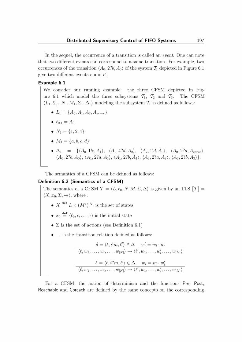
Distributed Supervisory Control of FIFO Systems 197
In the sequel, the occurrence of a transition is called an event. One can note
that two different events can correspond to a same transition. For example, two
occurrences of the transition 〈A0, 2?b, A0〉 of the system T1 depicted in Figure 6.1
give two different events e and e′.
Example 6.1
We consider our running example: the three CFSM depicted in Fig-
ure 6.1 which model the three subsystems T1, T2 and T3. The CFSM
〈L1, `0,1, N1,M1,Σ1,∆1〉 modeling the subsystem T1 is defined as follows:
• L1 = {A0, A1, A2, Aerror}
• `0,1 = A0
• N1 = {1, 2, 4}
• M1 = {a, b, c, d}
• ∆1 = {〈A0, 1!c, A1〉, 〈A1, 4?d,A2〉, 〈A2, 1!d,A0〉, 〈A0, 2?a,Aerror〉,〈A0, 2?b, A0〉, 〈A1, 2?a,A1〉, 〈A1, 2?b, A1〉, 〈A2, 2?a,A2〉, 〈A2, 2?b, A2〉}.
The semantics of a CFSM can be defined as follows:
Definition 6.2 (Semantics of a CFSM)
The semantics of a CFSM T = 〈L, `0, N,M,Σ,∆〉 is given by an LTS [[T ]] =
〈X, x0,Σ,→〉, where :
• X def= L× (M∗)|N | is the set of states
• x0def= 〈`0, ε, . . . , ε〉 is the initial state
• Σ is the set of actions (see Definition 6.1)
• → is the transition relation defined as follows:
δ = 〈`, i!m, `′〉 ∈ ∆ w′i = wi ·m
〈`, w1, . . . , wi, . . . , w|N |〉 → 〈`′, w1, . . . , w′i, . . . , w|N |〉
δ = 〈`, i?m, `′〉 ∈ ∆ wi = m · w′i
〈`, w1, . . . , wi, . . . , w|N |〉 → 〈`′, w1, . . . , w′i, . . . , w|N |〉
For a CFSM, the notion of determinism and the functions Pre, Post,
Reachable and Coreach are defined by the same concepts on the corresponding

198 Chapter 6
LTS (see section 1.2). In the sequel, we assume that T is deterministic.
Asynchronous Product. A distributed system T is generally composed of
several subsystems Ti (∀i ∈ [1, n]) acting in parallel. In our case, this global
system T is defined by a CFSM resulting from the asynchronous product of the
n subsystems Ti, also modeled by CFSM.
Definition 6.3 (Asynchronous Product)
Given n CFSM Ti = 〈Li, `0,i, Ni,Mi,Σi,∆i〉 (∀i ∈ [1, n]) with Li ∩ Lj = ∅(∀i 6= j ∈ [1, n]), their asynchronous product, denoted by T1|| . . . ||Tn, is defined
by a CFSM T = 〈L, `0, N,M,Σ,∆〉, where:
• L def= L1 × . . .× Ln
• `0def= `0,1 × . . .× `0,n
• N def= N1 ∪ . . . ∪ Nn. One can note that N1, . . . , Nn are not necessarily
disjoint; this allows the subsystems to communicate between them via
common queues.
• M def= M1 ∪ · · · ∪Mn
• Σdef= Σ1 ∪ · · · ∪ Σn
• ∆ is defined as follows: for each i ∈ [1, n], for each
transition δi = 〈`i, σi, `′i〉 ∈ ∆i, and for each location
`j ∈ Lj (∀j 6= i ∈ [1, n]), we create a new transition
〈〈`1, . . . , `i−1, `i, `i+1, . . . , `n〉, σi, 〈`1, . . . , `i−1, `′i, `i+1, . . . , `n〉〉
def∈ ∆.
Only the reachable part of T1|| . . . ||Tn is considered4.
Communication Architecture. The system T , that we want to control, is
defined by the asynchronous product of n CFSM Ti (∀i ∈ [1, n]) acting in parallel
and exchanging information through FIFO channels. In the sequel, to simplify
the notations, we suppose that the subsystems Ti use the same setM of messages.
We also assume that the communication architecture is point-to-point, meaning
that any subsystem Ti can send messages to any subsystem Tj (with Tj 6= Ti)
through a queue Qi,j. Thus, only Ti can write on Qi,j and only Tj can read on
4Note that the operator || can be seen as a commutative and associative binary operator.

Distributed Supervisory Control of FIFO Systems 199
this queue5. With this architecture, the set Ni of Ti (∀i ∈ [1, n]) is defined by
Ni = {Qi,j, Qj,i | (j 6= i) ∧ (1 ≤ j ≤ n)} and the set of actions Σi of Ti is disjoint
from the set of actions Σj of Tj (∀j 6= i ∈ [1, n]). Moreover, we suppose that
the message transfers between the subsystems are reliable and may suffer from
arbitrary non-zero delays, and that a global clock or perfectly synchronized local
clocks are not available.
Notations and Definitions. Given n CFSM Ti = 〈Li, `0,i, Ni,M,Σi,∆i〉 (∀i ∈[1, n]) communicating according to the architecture defined above, and a CFSM
T = T1|| . . . ||Tn = 〈L, `0, N,M,Σ,∆〉, we define the following notations:
• The projection Pi : Σ∗ → Σ∗i is defined as in (1.1).
• Let σ ∈ Σ be an action of T , Trans(σ)def= {〈`, σ1, `
′〉 ∈ ∆ |σ1 = σ} gives the
set of transitions of T labeled by the action σ.
• Let σ = σ1.σ2 . . . σn be a sequence of actions and ~ν, ~ν ′ ∈ L × (M∗)|N | be two
states of T , ∆(~ν, σ) gives the state which is reachable from ~ν by executing
the sequence σ. In other words, ∆(~ν, σ) = ~ν ′ if and only if ∃~ν0, ~ν1, . . . , ~νn ∈L × (M∗)|N | such that (i) ~ν0 = ~ν, (ii) ~νn = ~ν ′, and (iii) ∀i ∈ [1, n] : ~νi =
PostTσi(~νi−1). Since Ti is deterministic, only one state is reachable from the
state ~νi by firing the action σi.
• Let e be an event occurring in T and δe be the transition corresponding to
this event, ~νe−→ ~ν ′ means that the state ~ν ′ can be reached from ~ν by firing the
transition δe.
• Let δi = 〈`i, σi, `′i〉 ∈ ∆i be a transition of the subsystem Ti, global(δi)
def=
{〈〈`1, . . . , `i−1, `i, `i+1, . . . , `n〉, σi, 〈`1, . . . , `i−1, `′i, `i+1, . . . , `n〉〉 ∈ ∆ | ∀j 6= i ∈
[1, n] : `j ∈ Lj} gives the set of transitions of ∆ that are built from δi in the
asynchronous product T1|| . . . ||Tn (see the construction of ∆ in Definition 6.3).
We naturally extend this definition to sets of transitions: let D ⊆ ∆i be a set
of transitions, global(D)def=⋃
δi∈D global(δi).
• Let B ⊆ L × (M∗)|N | be a subset of states of T , and δi ∈ ∆i be a transition
of the subsystem Ti, by abuse of notation, we write ∆ \ ∆i instead of ∆ \global(∆i) and PostTδi
(B) (resp. PreTδi(B)) instead of PostTglobal(δi)
(B) (resp.
PreTglobal(δi)(B)).
5When Ti writes a message m on the queue Qi,j (i.e., it performs the action Qi,j !m), Tj canread this message by performing the action Qi,j?m.

200 Chapter 6
Moreover, we define the concept of execution as follows:
Definition 6.4 (Execution)
Given a CFSM T = 〈L, `0, N,M,Σ,∆〉, m events ei (∀i ∈ [1,m]), m+1 states
~νi (∀i ∈ [0,m]), and the transition δei(∀i ∈ [1,m]) corresponding to the event
ei, then an execution of T is a sequence s = ~ν0e1−→ ~ν1
e2−→ . . .em−→ ~νm where
~ν0 = 〈`0, ε, . . . , ε〉 is the initial state of T . In other words, for every i ∈ [1,m],
the state ~νi is reachable from the state ~νi−1 by the transition δei.
6.3 Framework and State Avoidance Control Problem
In this section, we define the framework, that we use, and the problem that we
want to solve. More precisely, in section 6.3.1, we define the control mecha-
nisms. Next, in section 6.3.2, we formally define the concepts of controller and
of controlled execution. Finally, in section 6.3.3, we define the distributed state
avoidance control problem.
6.3.1 Means of Control
The system to be controlled is composed of n subsystems Ti (∀i ∈ [1, n]) com-
municating according to the architecture defined in section 6.2. Classically, we
want to associate a local controller Ci (∀i ∈ [1, n]) with each subsystem Ti in
order to satisfy some control requirements. We suppose that the controllers can
communicate with each other by adding some information (e.g., their current
state, their state estimates, . . . ) to the messages exchanged by the subsystems
(see Figure 6.2, where C1 and C2 use the queues Q1,2 and Q2,1 of T1 and T2 to
exchange information6).
Following the Ramadge & Wonham’s theory [RW89], Ci (∀i ∈ [1, n]) interacts
with Ti in a feedback manner: the controller Ci observes the last action7 fired by
Ti and computes, from this observation and the information received from the
other controllers (this information is actually state estimates), a set of actions
that the subsystem Ti cannot fire in order to ensure the desired properties on the
global system. Moreover, we suppose that the local controller Ci synchronously
communicates with Ti. This assumption is realistic, since they generally reside
in the same site.
6We duplicate the queues in Figure 6.2 to emphasize the fact that the controllers canexchange information.
7Ci observes the actions fired by Ti in order to have a better knowledge about Ti.

Distributed Supervisory Control of FIFO Systems 201
and
T1 T2
C1 C2
Synchronous Communication
Synchronous Communication
Queues
Queues
System to be controlled
System under the control of
Q1,2
Q1,2
Q2,1
Q2,1
C1 C2
Figure 6.2 - Control architecture of a distributed system composed of two sub-
systems T1 and T2.
Moreover, as usual, the set of actions Σi of Ti is partitioned into the set of
controllable actions Σi,c, that can be forbidden by Ci, and the set of uncontrollable
actions Σi,uc, that cannot be forbidden by Ci. The subsets Σ1,c, . . . ,Σn,c are
disjoint, because Σi ∩ Σj = ∅ (∀i 6= j ∈ [1, n]). Without loss of generality, we
assume that:
• inputs are uncontrollable, and
• outputs are controllable.
Indeed, in a reactive system, the inputs cannot generally be controlled, whereas
the outputs can be controlled.
The set of actions, that can be controlled by at least one controller, is denoted
by Σc and is defined by Σcdef=⋃n
i=1 Σi,c and the set of actions, that cannot be
controlled, is denoted by Σuc and is defined by Σucdef= Σ \Σc =
⋃ni=1 Σi,uc. That
also induces a partition of the set of transitions ∆i into the set ∆i,c and the set
∆i,uc: the transition 〈`, σ, `′〉def∈ ∆i,c, if the action σ ∈ Σi,c, and the transition
〈`, σ, `′〉def∈ ∆i,uc, if the action σ ∈ Σi,uc. The set of transitions ∆ is similarly
partitioned into the set ∆c and the set ∆uc.

202 Chapter 6
Partial Observation. In the architecture we propose, the local controllers have
only a partial observation of the global system. It is due to the fact that a local
controller Ci cannot observe the internal state of the subsystems Tj (∀j 6= i ∈[1, n]) and the content of the FIFO channels.
6.3.2 Distributed Controller and Controlled Execution
The local controllers aim at restricting the behavior of the subsystems to ensure
the desired properties. We formally define the local controllers Ci (∀i ∈ [1, n]) as
follows:
Definition 6.5 (Local Controller)
Given n subsystems Ti = 〈Li, `0,i, Ni,M,Σi,∆i〉 (∀i ∈ [1, n]) communicat-
ing according to the architecture defined in section 6.2, and a CFSM T =
T1|| . . . ||Tn = 〈L, `0, N,M,Σ,∆〉, a local controller Ci, which interacts with Ti
in order to restrict the behavior of this subsystem, is a pair Cidef= 〈Si, Ei〉,
where8:
• Si : 2L×(M∗)|N| → 2Σc is a supervisory function which defines, for each
P ∈ 2L×(M∗)|N|, a set Si(P ) of controllable actions that Ti cannot execute
when P is the estimate of the current state of T computed by Ci.
• Ei ⊆ L× (M∗)|N | is a set of states, in which the system T cannot begin
its execution.
In our control algorithm, we shall use the method defined in section 6.4 to com-
pute, during the execution of the system, the state estimate P of Ci.Based on Definition 6.5, a distributed controller is defined as follows:
Definition 6.6 (Distributed Controller)
Given n subsystems Ti = 〈Li, `0,i, Ni,M,Σi,∆i〉 (∀i ∈ [1, n]) communi-
cating according to the architecture defined in section 6.2, and a CFSM
T = T1|| . . . ||Tn = 〈L, `0, N,M,Σ,∆〉, a distributed controller Cdi is defined
by a tuple Cdidef= 〈Ci〉ni=1 where Ci (∀i ∈ [1, n]) is a local controller (see Defini-
tion 6.5).
8Since the system T has only one initial state, we could define a local controller Ci withoutthe component Ei, but we keep it to remain coherent with the definitions of controller givenin the previous chapters.

Distributed Supervisory Control of FIFO Systems 203
The concept of controlled execution characterizes the executions that can occur
in a system T under the control of a distributed controller Cdi.
Definition 6.7 (Controlled Execution)
Given n subsystems Ti = 〈Li, `0,i, Ni,M,Σi,∆i〉 (∀i ∈ [1, n]) communicating
according to the architecture defined in section 6.2, a CFSM T = T1|| . . . ||Tn =
〈L, `0, N,M,Σ,∆〉, a distributed controller Cdi = 〈Ci〉ni=1 (for each i ∈ [1, n],
Ci = 〈Si, Ei〉), an execution s = ~ν0e1−→ ~ν1
e2−→ . . .em−→ ~νm of T , and the
transition δej= 〈`, σej
, `′〉 (∀j ∈ [1,m]) corresponding to the event ej, then s
is a controlled execution of the system T under the control of Cdi if it satisfies
the following conditions:
• the initial state ~ν0 = 〈`0,1, . . . , `0,n, ε, . . . , ε〉 does not belong to Ei (∀i ∈[1, n]).
• for every k ∈ [1,m], if δek∈ ∆i, then, when the system T reaches the
state ~νk−1, the controller Ci has an estimate P of the current state of Tsuch that σek
6∈ Si(P ). In other words, Ci allows the action σekwhen the
system T reaches ~νk−1
We shall see later on, how such a state estimate P can be computed.
6.3.3 Definition of the Control Problem
We define the problem we are interested in as follows:
Problem 6.1 (Distributed State Avoidance Control Problem)
Given n subsystems Ti = 〈Li, `0,i, Ni,M,Σi,∆i〉 (∀i ∈ [1, n]) communicating
according to the architecture defined in section 6.2, a CFSM T = T1|| . . . ||Tn =
〈L, `0, N,M,Σ,∆〉, and a set of forbidden states Bad ⊆ L× (M∗)|N |, the dis-
tributed state avoidance control problem (distributed problem for short) consists
in synthesizing a distributed controller Cdi = 〈Ci〉ni=1 = 〈〈Si, Ei〉〉ni=1 such that
(i) the initial state ~ν0 = 〈`0,1, . . . , `0,n, ε, . . . , ε〉 of T does not belong to Ei
(∀i ∈ [1, n]), and (ii) each controlled execution ~ν0e1−→ ~ν1
e2−→ . . .em−→ ~νm of the
system T under the control of Cdi does not reach Bad i.e, the state ~νm 6∈ Bad.
The first condition ensures that the distributed controller is not trivial and the
second one ensures that Bad is not reachable.

204 Chapter 6
Proposition 6.1
The distributed problem is undecidable.
Intuitively, this proposition holds, because the reachability is undecidable in the
model of CFSM.
As explained in section 6.1 and as shown in Definition 6.7, the local controllers
Ci define their control policy from an estimate of the current state of the global
system T that they compute during the execution of this system. In the next
section, we explain how they compute this state estimate.
6.4 State Estimates of Distributed Systems
In this section, we present our algorithm that computes estimates of the current
state of a distributed system. This algorithm is used, in section 6.5, by our
control algorithm which synthesizes distributed controllers for the distributed
problem. But, before presenting this algorithm, we recall the concept of vector
clocks [Mat89] that we use to compute state estimates.
6.4.1 Instrumentation
In a centralized system, it is quite easy to determine if an event precedes another
one, since all events are emitted by the same process. A logical clock, which
counts the number of events, can be used to time-stamp the events and the order
of two events can then be determined by comparing the value of their respective
time-stamp.
In a distributed system, events emitted by a same process are ordered, while
events emitted by different processes are generally not. However, when the con-
current processes communicate, additional ordering information can be obtained.
In this case, the communication scheme can be used to obtain a partial order
on the events of the system. In practice, vectors of logical clocks, called Vector
clocks [Lam78], can be used to time-stamp the events of a distributed system.
The order of two events can then be determined by comparing the value of their
respective vector clocks. However, these vector clocks can be incomparable. In
this case, the exact order in which the events occur cannot be determined. Vector
clocks are formally defined as follows:
Distributed Supervisory Control of FIFO Systems 205
Definition 6.8 (Vector Clocks)
Let 〈X,v〉 be a partially ordered set, a vector clock mapping of width n is a
function V : X → (N0)n such that:
∀x1, x2 ∈ X : (x1 v x2)⇔ (V (x1) ≤ V (x2)) (6.1)
In general, for a distributed system composed of n processes, the partial order
on events is represented by a vector clock mapping of width n. The method for
computing this vector clock mapping depends on the communication scheme of
the distributed system. CFSM communicate via message passing and hence we
present, below, an algorithm [Mat89] that computes vector clock mappings for
this communication scheme. We also present some properties [Mat89] related to
this concept of vector clocks.
Computation of a Vector Clock Mapping. In a distributed system, when
the processes asynchronously communicate via message passing, the sending of
a message always precedes its reception. This information can then be used to
determine a partial order, called causality (or happened-before) relation, on the
events of the system. This relation is formally defined as follows:
Definition 6.9 (Causality Relation)
Let Ei (∀i ∈ [1, n]) be the set of events occurring in an execution of Ti and
E =⋃
i∈[1,n]Ei, the causality (or happened-before) relation ≺c⊆ E × E is the
smallest transitive relation satisfying the following conditions:
• if ei 6= ej ∈ Ei (i.e., these events occur in the same process Ti) and if ei
comes before ej in the execution, then ei ≺c ej.
• if ei ∈ Ei is an output event and if ej ∈ Ej is the corresponding input
event, then ei ≺c ej.
One can note that ≺c is irreflexive. When ei ≺c ej, we say that ej causally
depends on ei (or that ei happened-before ej). Notice that a total order on the
events of a distributed system can be obtained when one supposes the existence
of a global clock or perfectly synchronized local clocks. But, in our framework,
we have not this assumption.
The vector clock mapping for this relation can be obtained by using the

206 Chapter 6
Algorithm 5: MatternAlgorithm(Ti, Vi, e)
input : A subsystem Ti (with i ∈ [1, n]), the vector clock Vi of Ti, and an evente occurring in Ti.
output: The vector clock Vi after the occurrence of e.begin1
Vi[i]← Vi[i] + 12
if e corresponds to an output transition sending the message m to Tj then3
send 〈m,Vi〉 to Tj instead of m4
else if e corresponds to an input transition reading the message 〈m,Vj〉5
coming from Tj thenfor k ← 1 to n do6
Vi[k]←max(Vi[k], Vj [k])7
return (Vi)8
end9
Mattern’s algorithm [Mat89] (see Algorithm 5). In this algorithm, each process
Ti (∀i ∈ [1, n]) has a vector clock Vi ∈ (N0)n of width n. Each element Vi[j]
(∀j ∈ [1, n]) is a counter which represents the knowledge of Ti regarding Tj and
which can roughly be interpreted as follows: Ti knows that Tj has executed at
least Vi[j] events. More precisely, Vi[j] gives the number of events of Tj that
happened-before the most recent event of Ti. Initially, each component of the
vector Vi (∀i ∈ [1, n]) is set to 0. Next, when an event e occurs in Ti, the vector
clock Vi is updated as follows (see Algorithm 5): first, Vi[i] is incremented (i.e.,
Vi[i] ← Vi[i] + 1) to indicate that a new event occured in Ti and next two cases
are considered:
• if e consists in sending the message m to Tj, the vector clock Vi is attached to
m and this information is sent to Tj (see lines 3 and 4).
• if e corresponds to the reception of the message m tagged with the vector clock
Vj, then Vi is set to the component-wise maximum of Vi and Vj. This allows
us to take into account the fact that any event, that precedes the sending of
m, should also precede the event e (see lines 5, 6 and 7).
In the sequel, the vector clock Vi, computed after the occurrence of an event
e in Ti, is denoted by Vi(e).

Distributed Supervisory Control of FIFO Systems 207
1!cT1
T2
T3
[1, 0, 0]
[1, 1, 0] [1, 2, 0] [1, 3, 0]
[1, 3, 1] [1, 3, 2]
[2, 3, 2] [3, 3, 2] [4, 3, 2]
[3, 4, 2]1?c 2!a 3!d
3?d 4!d
4?d 1!d
1?d
2?a
Figure 6.3 - Illustration of the concept of vector clocks.
Example 6.2
Let us illustrate this mechanism on our running example (see Figure 6.1). We
consider the following sequence of actions (see Figure 6.3):
• The subsystem T1 performs the action A01!c→ A1 and attaches its vector
clock V1 = [1, 0, 0] to the message c.
• The subsystem T2 performs the action B01?c→ B1 and updates its vector
clock: V2 = [1, 1, 0].
• The subsystem T2 performs the action B12!a→ B2 and attaches its vector
clock V2 = [1, 2, 0] to the message a.
• The subsystem T2 performs the action B23!d→ B3 and attaches its vector
clock V2 = [1, 3, 0] to the message d.
• The subsystem T3 performs the action D03?d→ D1 and updates its vector
clock: V3 = [1, 3, 1].
• The subsystem T3 performs the action D14!d→ D0 and attaches its vector
clock V3 = [1, 3, 2] to the message d.
208 Chapter 6
• The subsystem T1 performs the action A14?d→ A2 and updates its vector
clock: V1 = [2, 3, 2].
• The subsystem T1 performs the action A21!d→ A0 and attaches its vector
clock V1 = [3, 3, 2] to the message d.
• The subsystem T2 performs the action B31?d→ B0 and updates its vector
clock: V2 = [3, 4, 2].
• The subsystem T1 performs the action A02?a→ Aerror and updates its
vector clock: V1 = [4, 3, 2]. Note that the vector clock V2 attached to
this input is out of date, since V2 = [1, 2, 0] and V1 = [3, 3, 2] before this
input.
Propositions. The following proposition proves the correctness of the vector
clock mapping computed by the Mattern’s algorithm for the relation ≺c:
Proposition 6.2 ([Mat89])
Given n subsystems Ti (∀i ∈ [1, n]) and two events e1 6= e2 occurring respec-
tively in Ti and Tj (i can be equal to j), we have the following equivalence:
e1 ≺c e2 if and only if Vi(e1) ≤ Vj(e2)
In the sequel, we will need the following proposition:
Proposition 6.3
Given n subsystems Ti (∀i ∈ [1, n]) and three events ei 6= ej 6= ek occurring
respectively in Ti, Tj and Tk (we can have Ti = Tj), if ek 6≺c ej and ei ≺c ej,
then ek 6≺c ei.
Proof
We suppose that ek ≺c ei. Since ek 6≺c ej, there exists a number ` ∈ [1, n] such
that Vk(ek)[`] > Vj(ej)[`]. Moreover, Vk(ek)[`] > Vi(ei)[`], because Vi(ei)[m] ≤Vj(ej)[m] for each m ∈ [1, n] (due to ei ≺c ej). But it is a contradiction with
ek ≺c ei, because this relation implies that Vk(ek)[m] ≤ Vi(ei)[m] for each
m ∈ [1, n].
Distributed Supervisory Control of FIFO Systems 209
6.4.2 Computation of State Estimates
In our control algorithm, defined in section 6.5, each local controller must com-
pute, during the execution of the distributed system, an estimate of the current
state of the system to define its control policy. In this section, we explain how
this state estimate is computed.
Let Ti = 〈Li, `0,i, Ni,M,Σi,∆i〉 (∀i ∈ [1, n]) be n CFSM communicating
according to the architecture defined in section 6.2, and T = T1|| . . . ||Tn =
〈L, `0, N,M,Σ,∆〉 be a CFSM. Our state estimate algorithm computes, for each
local controller Ci and for each event occurring in the subsystem Ti, a vector
clock Vi and a state estimate CSi that contains the current state of the global
system T and any future state that can be reached from this current state by
firing actions that do not belong to Ti. This computation obviously depends on
the information that Ci receives: as a reminder, Ci observes the last action fired
by Ti (note that since Ti is deterministic, Ci can infer the fired transition) and can
receive from the other controllers Cj their state estimate CSj and their vector
clock Vj. Our state estimate algorithm proceeds as follows. When the subsystem
Ti performs an action, the following operations are performed:
• If it is an output message m, Ti attaches the vector clock Vi and the state
estimate CSi of Ci to this message. Next, Ci receives the action fired by Ti
and infers the fired transition. It then uses this information to update its state
estimate CSi.
• If it is an input message m sent by Tj, Ci receives the action fired by Ti and
the information sent by Tj i.e., the state estimate CSj and the vector clock
Vj of Cj. It computes its new state estimate from these elements.
In both cases, the computation of the new state estimate CSi depends on the
computation of reachable states. In this section, we assume that we have an op-
erator that can compute an approximation of the reachable states (as a reminder,
the computation of the reachable states is undecidable is the model of CFSM).
We will explain in section 6.5 how such an operator can be obtained.
6.4.2.1 State Estimate Algorithm
Our algorithm, that computes estimates of the current state of a distributed
system, is composed of three subalgorithms:
• initialEstimate: computes, for each local controller, its initial state estimate.
It is only used when the system starts its execution.
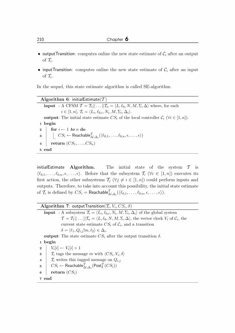
210 Chapter 6
• outputTransition: computes online the new state estimate of Ci after an output
of Ti.
• inputTransition: computes online the new state estimate of Ci after an input
of Ti.
In the sequel, this state estimate algorithm is called SE-algorithm.
Algorithm 6: initialEstimate(T )
input : A CFSM T = T1|| . . . ||Tn = 〈L, `0, N, M, Σ,∆〉 where, for eachi ∈ [1, n], Ti = 〈Li, `0,i, Ni,M,Σi,∆i〉.
output: The initial state estimate CSi of the local controller Ci (∀i ∈ [1, n]).begin1
for i← 1 to n do2
CSi ← ReachableT∆\∆i(〈`0,1, . . . , `0,n, ε, . . . , ε〉)3
return (CS1, . . . , CSn)4
end5
initialEstimate Algorithm. The initial state of the system T is
〈`0,1, . . . , `0,n, ε, . . . , ε〉. Before that the subsystem Ti (∀i ∈ [1, n]) executes its
first action, the other subsystems Tj (∀j 6= i ∈ [1, n]) could perform inputs and
outputs. Therefore, to take into account this possibility, the initial state estimate
of Ti is defined by CSi = ReachableT∆\∆i(〈`0,1, . . . , `0,n, ε, . . . , ε〉).
Algorithm 7: outputTransition(Ti, Vi, CSi, δ)
input : A subsystem Ti = 〈Li, `0,i, Ni,M, Σi,∆i〉 of the global systemT = T1|| . . . ||Tn = 〈L, `0, N, M, Σ,∆〉, the vector clock Vi of Ci, thecurrent state estimate CSi of Ci, and a transitionδ = 〈`1, Qi,j !m, `2〉 ∈ ∆i.
output: The state estimate CSi after the output transition δ.begin1
Vi[i]← Vi[i] + 12
Ti tags the message m with 〈CSi, Vi, δ〉3
Ti writes this tagged message on Qi,j4
CSi ← ReachableT∆\∆i(PostTδ (CSi))5
return (CSi)6
end7
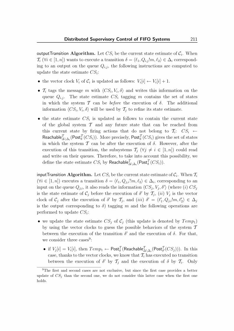
Distributed Supervisory Control of FIFO Systems 211
outputTransition Algorithm. Let CSi be the current state estimate of Ci. When
Ti (∀i ∈ [1, n]) wants to execute a transition δ = 〈`1, Qi,j!m, `2〉 ∈ ∆i correspond-
ing to an output on the queue Qi,j, the following instructions are computed to
update the state estimate CSi:
• the vector clock Vi of Ci is updated as follows: Vi[i]← Vi[i] + 1.
• Ti tags the message m with 〈CSi, Vi, δ〉 and writes this information on the
queue Qi,j. The state estimate CSi tagging m contains the set of states
in which the system T can be before the execution of δ. The additional
information 〈CSi, Vi, δ〉 will be used by Tj to refine its state estimate.
• the state estimate CSi is updated as follows to contain the current state
of the global system T and any future state that can be reached from
this current state by firing actions that do not belong to Ti: CSi ←ReachableT∆\∆i
(PostTδ (CSi)). More precisely, PostTδ (CSi) gives the set of states
in which the system T can be after the execution of δ. However, after the
execution of this transition, the subsystems Tj (∀j 6= i ∈ [1, n]) could read
and write on their queues. Therefore, to take into account this possibility, we
define the state estimate CSi by ReachableT∆\∆i(PostTδ (CSi)).
inputTransition Algorithm. Let CSi be the current state estimate of Ci. When Ti
(∀i ∈ [1, n]) executes a transition δ = 〈`1, Qj,i?m, `2〉 ∈ ∆i, corresponding to an
input on the queue Qj,i, it also reads the information 〈CSj, Vj, δ′〉 (where (i) CSj
is the state estimate of Cj before the execution of δ′ by Tj, (ii) Vj is the vector
clock of Cj after the execution of δ′ by Tj, and (iii) δ′ = 〈`′1, Qj,i!m, `′2〉 ∈ ∆j
is the output corresponding to δ) tagging m and the following operations are
performed to update CSi:
• we update the state estimate CSj of Cj (this update is denoted by Temp1)
by using the vector clocks to guess the possible behaviors of the system Tbetween the execution of the transition δ′ and the execution of δ. For that,
we consider three cases9:
• if Vj[i] = Vi[i], then Temp1 ← PostTδ (ReachableT∆\∆i(PostTδ′(CSj))). In this
case, thanks to the vector clocks, we know that Ti has executed no transition
between the execution of δ′ by Tj and the execution of δ by Ti. Only
9The first and second cases are not exclusive, but since the first case provides a betterupdate of CSj than the second one, we do not consider this latter case when the first oneholds.

212 Chapter 6
Algorithm 8: inputTransition(Ti, Vi, CSi, δ)
input : A subsystem Ti = 〈Li, `0,i, Ni,M, Σi,∆i〉 of the global systemT = T1|| . . . ||Tn = 〈L, `0, N, M, Σ,∆〉, the vector clock Vi of Ci, thecurrent state estimate CSi of Ci and a transitionδ = 〈`1, Qj,i?m, `2〉 ∈ ∆i. The message m is tagged with the triple〈CSj , Vj , δ
′〉 where (i) CSj is the state estimate of Cj before theexecution of δ′ by Tj , (ii) Vj is the vector clock of Cj after theexecution of δ′ by Tj , and (iii) δ′ = 〈`′1, Qj,i!m, `′2〉 ∈ ∆j is the outputcorresponding to δ.
output: The state estimate CSi after the input transition δ.begin1
\\ We consider three cases to update CSj2
if Vj [i] = Vi[i] then3
Temp1 ← PostTδ (ReachableT∆\∆i(PostTδ′(CSj)))4
else if Vj [j] > Vi[j] then5
Temp1 ← PostTδ (ReachableT∆\∆i(ReachableT∆\∆j
(PostTδ′(CSj))))6
else7
Temp1 ← PostTδ (ReachableT∆(PostTδ′(CSj)))8
CSi ← PostTδ (CSi) \\ We update CSi9
CSi ← CSi ∩ Temp110
\\ We intersect the updates of CSi and CSj (i.e., Temp1) to obtain the11
\\ new state estimate CSi12
Vi[i]← Vi[i] + 113
for k ← 1 to n do14
Vi[k]←max(Vi[k], Vj [k])15
return (CSi)16
end17

Distributed Supervisory Control of FIFO Systems 213
transitions in ∆\∆i could thus have occurred during this period and we then
update CSj as follows. We compute PostTδ′(CSj) to take into account the
execution of δ′ by Tj, ReachableT∆\∆i(PostTδ′(CSj)) to take into account the
transitions that could occur between the execution of δ′ and the execution
of δ, and finally PostTδ (ReachableT∆\∆i(PostTδ′(CSj))) to take into account the
execution of δ by Ti.
• else if Vj[j] > Vi[j], then Temp1 ←PostTδ (ReachableT∆\∆i
(ReachableT∆\∆j(PostTδ′(CSj)))). Indeed, in this
case, we can prove (see the proof of Proposition 6.4) that the transitions
executed between the execution of δ′ and the execution of δ can be
reordered in order to execute the transitions of ∆i before the ones of ∆j.
So, in this reordered sequence, we know that, after the execution of δ,
only transitions in ∆ \ ∆j could occur followed by transitions in ∆ \ ∆i.
Intuitively, this reordering is possible, because there is no causal relation
between the events of Ti and the events of Tj, that have occurred between
δ′ and δ.
• else Temp1 ← PostTδ (ReachableT∆(PostTδ′(CSj))). Indeed, in this case, the
vector clocks do not allow us to deduce information regarding the behavior
of the system T between the execution of the transition δ′ and the execution
of δ. Therefore, to have a correct state estimate, we update CSj by taking
into account all possible behaviors of the system T between the execution
of δ′ and the execution of δ. One can note that Lemma 6.1 (see below)
shows that the set Temp1 computed in the second case is better that the
one computed in this third case.
• we update the state estimate CSi to take into account the execution of the
input transition δ: CSi ← PostTδ (CSi).
• we have two different state estimates: Temp1 and CSi. Thus, we intersect
them to obtain a better state estimate: CSi ← CSi ∩ Temp1.
• we update the vector clock Vi to take into account the execution of δ: Vi[i]←Vi[i] + 1.
• we update the vector clock Vi by using the information given by Vj: Vi[k] ←max(Vi[k], Vj[k]) for each k ∈ [1, n].
Now, we prove that the set Temp1 computed at the line 6 of Algorithm 8 is
more accurate than the one computed at the line 8 of Algorithm 8.

214 Chapter 6
!11
!21
!a
!b
!12
!22!b
!23 !24 !25
!15!14!13?b ?b!a
?a ?a
T1
T2
Figure 6.4 - System where ReachableT∆\∆1(ReachableT∆\∆2
(B)) ⊂ ReachableT∆(B).
Lemma 6.1
Given n subsystems Ti = 〈Li, `0,i, Ni,M,Σi,∆i〉 (∀i ∈ [1, n]) communicating
according to the architecture defined in section 6.2, a CFSM T = T1|| . . . ||Tn =
〈L, `0, N,M,Σ,∆〉, i 6= j ∈ [1, n], and a set B ⊆ L × (M∗)|N |, then
ReachableT∆\∆i(ReachableT∆\∆j
(B)) ⊆ ReachableT∆(B).
Proof
This proposition holds because ∆ \∆i ⊆ ∆ and ∆ \∆j ⊆ ∆.
Moreover, the following example shows that, in some cases, we can have
ReachableT∆\∆i(ReachableT∆\∆j
(B)) ⊂ ReachableT∆(B).
Example 6.3
Let T1 = 〈L1, `0,1, N1,M,Σ1,∆1〉 and T2 = 〈L2, `0,2, N2,M,Σ2,∆2〉 be
two subsystems communicating according to the architecture defined in
section 6.2 (see Figure 6.4), and T = T1||T2 = 〈L, `0, N,M,Σ,∆〉.Given a state 〈`1, `2, w1, w2〉 of T , (i) `1 (resp. `2) gives the cur-
rent location of T1 (resp. T2) and (ii) w1 (resp. w2) gives the con-
tent of the queue Q1,2 (resp. Q2,1). We define B as follows: B =
{〈`11, `21, ε, ε〉}. The set ReachableT∆\∆1(ReachableT∆\∆2
(B)) = {〈`11, `21, ε, ε〉,〈`11, `22, ε, b〉, 〈`12, `21, a, ε〉, 〈`12, `22, a, b〉, 〈`12, `23, ε, b〉, 〈`12, `24, ε, bb〉}. This set is
strictly included in ReachableT∆(B) = {〈`11, `21, ε, ε〉, 〈`12, `21, a, ε〉, 〈`11, `22, ε, b〉,〈`12, `22, a, b〉, 〈`13, `22, a, ε〉, 〈`14, `22, aa, ε〉, 〈`12, `23, ε, b〉, 〈`12, `24, ε, bb〉, 〈`13, `23, ε, ε〉,〈`14, `23, a, ε〉, 〈`13, `24, ε, b〉, 〈`14, `24, a, b〉, 〈`15, `24, a, ε〉, 〈`14, `25, ε, b〉, 〈`15, `25, ε, ε〉}.
6.4.2.2 Properties
Notations. Let s = ~ν0e1−→ ~ν1
e2−→ . . .em−→ ~νm be an execution of the global system
T . When the subsystem Ti executes an event ek (with k ∈ [1,m]) of this sequence,

Distributed Supervisory Control of FIFO Systems 215
the state estimate, computed by Ci at this step, is denoted by CSti , where t is
the number of events executed by Ti in the subsequence ~ν0e1−→ ~ν1
e2−→ . . .ek−→ ~νk.
However, to be more concise in our proofs, we use an abuse of notation: when an
event ek is executed in the sequence s, the state estimate of each subsystem Ti is
denoted by CSki (in this way, we do not need to introduce, for each subsystem, a
parameter giving the number of events that is has executed). This state estimate
is then defined in the following way:
• if ek has not been executed by Ti, then CSki
def= CSk−1
i ,
• otherwise, the value of CSki is computed by Algorithms 7 or 8 from the state
estimate CSk−1i .
Definitions. We define the concepts of complete and sound algorithms as fol-
lows:
Definition 6.10 (Complete Algorithm)
Given n subsystems Ti = 〈Li, `0,i, Ni,M,Σi,∆i〉 (∀i ∈ [1, n]) communicating
according to the architecture defined in section 6.2, a CFSM T = T1|| . . . ||Tn =
〈L, `0, N,M,Σ,∆〉, and an execution ~ν0e1−→ ~ν1
e2−→ . . .em−→ ~νm of T (as a re-
minder, the initial state ~ν0 = 〈`0,1, . . . , `0,n, ε, . . . , ε〉), a state estimate algo-
rithm for T is complete if and only if the current state ~νm belongs to the state
estimate CSmi (∀i ∈ [1, n]).
The completeness of an algorithm refers to the fact that the current state of the
global system is always included in the state estimate.
Definition 6.11 (Sound Algorithm)
Given n subsystems Ti = 〈Li, `0,i, Ni,M,Σi,∆i〉 (∀i ∈ [1, n]) communicating
according to the architecture defined in section 6.2, a CFSM T = T1|| . . . ||Tn =
〈L, `0, N,M,Σ,∆〉, an execution s = ~ν0e1−→ ~ν1
e2−→ . . .em−→ ~νm of T , and
the transition 〈`ek, σek
, `′ek〉 (∀k ∈ [1,m]) corresponding to the event ek, a
state estimate algorithm for T is sound if and only if ∀i ∈ [1, n] : CSmi ⊆⋃
σ∈P−1i (Pi(σe1 .σe2 ...σem )) ∆(~ν0, σ), where ~ν0 = 〈`0,1, . . . , `0,n, ε, . . . , ε〉 is the initial
state of T .
When Ti executes an action, Ci receives the fired action. Therefore, the
observation of the system Ti allows the local controller Ci to know that the
system T has executed a sequence of actions σ ∈ P−1i (Pi(σe1 .σe2 . . . σem)) to
reach the state ~νm. The soundness of an algorithm refers to the fact that a state

216 Chapter 6
is included in the state estimate of Ci only if it can be reached by one of these
sequences σ.
Properties. As explained above, we assume that we can compute an approx-
imation of the reachable states. In this part, we present the properties of our
state estimate algorithm w.r.t. the kind of used approximations.
Proposition 6.4
Given n subsystems Ti = 〈Li, `0,i, Ni,M,Σi,∆i〉 (∀i ∈ [1, n]) communi-
cating according to the architecture defined in section 6.2, and a CFSM
T = T1|| . . . ||Tn = 〈L, `0, N,M,Σ,∆〉, SE-algorithm is complete, if we com-
pute an overapproximation of the reachable states.
The proof is given in section 6.6. If we compute an underapproximation of
the reachable states, our state estimate algorithm is not complete and hence,
in section 6.5, we define an effective algorithm for the distributed problem by
computing overapproximations of the reachable states.
Proposition 6.5
Given n subsystems Ti = 〈Li, `0,i, Ni,M,Σi,∆i〉 (∀i ∈ [1, n]) communi-
cating according to the architecture defined in section 6.2, and a CFSM
T = T1|| . . . ||Tn = 〈L, `0, N,M,Σ,∆〉, SE-algorithm is sound, if we compute
an underapproximation of the reachable states.
The proof is given in section 6.6. If we compute an overapproximation of the
reachable states, our state estimate algorithm is not sound.
Remark 6.1 (Improvements of the State Estimates)
Our state estimate algorithm can be improved by informing the subsystems
of the reading of a message. More precisely, when a subsystem Tj executes
an input transition δ = 〈`j, Qi,j?m, `′j〉 (with i 6= j ∈ [1, n]), it sends an odd
message tagged with this transition δ, the state estimate CSj and the vector
clock Vj on the queue Qj,k (∀k 6= j ∈ [1, n]). When the subsystem Tk reads
this message, its local controller Ck can refine its state estimate from this
information. For that, it first updates its state estimate CSk by taking into
account the reading of m on the queue Qi,j: CSk ← PostTδ (CSk). Next, it
updates CSj by using the method based on vector clocks which is defined in

Distributed Supervisory Control of FIFO Systems 217
Algorithm 8. Finally, it intersects these two sets to obtain the new state esti-
mate CSk. It can be proved that the properties of soundness and completeness
remain valid with this improvement.
6.5 Computation by Means of Abstract Interpretation of
Distributed Controllers for the Distributed Problem
In this section, we first define a semi-algorithm for the distributed problem. Next,
we explain how to extend it by using abstract interpretation techniques to obtain
an effective algorithm.
6.5.1 Semi-algorithm for the Distributed Problem
Our algorithm, which synthesizes a distributed controller Cdi for the distributed
problem, is composed of two parts:
1. Offline part: we compute, using a fixpoint equation, the set I(Bad) of
states of the global system T that can lead to Bad by a sequence of un-
controllable transitions. Next, we compute, for each local controller Ci, a
control function Fi which gives, for each action σ of Ti, the set of states of
T that can lead to I(Bad) by a transition labeled by σ. This information
is used by Ci, in the online part, to define its control policy. This part is
computed offline.
2. Online part: During the execution of the system T , each local controller
Ci uses SE-algorithm to obtain its own state estimate CSi and computes,
from this information and its control function Fi (computed in the offline
part), the actions to be forbidden. Roughly, Ci forbids an action σ in a
state ~ν of T if ~ν belongs to CSi and if Fi asks to forbid σ in ~ν.
These two parts are formalized as follows.
Offline Part. The set I(Bad) of states of T leading uncontrollably to Bad is
given by CoreachT∆uc(Bad) which, as a reminder, is defined by CoreachT∆uc
(Bad) =⋃n≥0(PreT∆uc
)n(Bad) (see Definition 1.9). This set of states cannot always be
computed, because the coreachability is undecidable in the model of CFSM.
So, we use abstract interpretation techniques to overapproximate it. However,
to compute this overapproximation, we must characterize the set I(Bad) by a
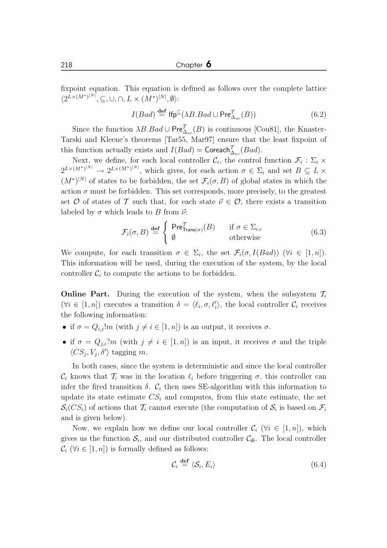
218 Chapter 6
fixpoint equation. This equation is defined as follows over the complete lattice
〈2L×(M∗)|N|,⊆,∪,∩, L× (M∗)|N |, ∅〉:
I(Bad)def= lfp⊆(λB.Bad ∪ PreT∆uc
(B)) (6.2)
Since the function λB.Bad ∪ PreT∆uc(B) is continuous [Cou81], the Knaster-
Tarski and Kleene’s theorems [Tar55, Mar97] ensure that the least fixpoint of
this function actually exists and I(Bad) = CoreachT∆uc(Bad).
Next, we define, for each local controller Ci, the control function Fi : Σi ×2L×(M∗)|N| → 2L×(M∗)|N|
, which gives, for each action σ ∈ Σi and set B ⊆ L ×(M∗)|N | of states to be forbidden, the set Fi(σ,B) of global states in which the
action σ must be forbidden. This set corresponds, more precisely, to the greatest
set O of states of T such that, for each state ~ν ∈ O, there exists a transition
labeled by σ which leads to B from ~ν:
Fi(σ,B)def=
{PreTTrans(σ)(B) if σ ∈ Σi,c
∅ otherwise(6.3)
We compute, for each transition σ ∈ Σi, the set Fi(σ, I(Bad)) (∀i ∈ [1, n]).
This information will be used, during the execution of the system, by the local
controller Ci to compute the actions to be forbidden.
Online Part. During the execution of the system, when the subsystem Ti
(∀i ∈ [1, n]) executes a transition δ = 〈`i, σ, `′i〉, the local controller Ci receives
the following information:
• if σ = Qi,j!m (with j 6= i ∈ [1, n]) is an output, it receives σ.
• if σ = Qj,i?m (with j 6= i ∈ [1, n]) is an input, it receives σ and the triple
〈CSj, Vj, δ′〉 tagging m.
In both cases, since the system is deterministic and since the local controller
Ci knows that Ti was in the location `i before triggering σ, this controller can
infer the fired transition δ. Ci then uses SE-algorithm with this information to
update its state estimate CSi and computes, from this state estimate, the set
Si(CSi) of actions that Ti cannot execute (the computation of Si is based on Fi
and is given below).
Now, we explain how we define our local controller Ci (∀i ∈ [1, n]), which
gives us the function Si, and our distributed controller Cdi. The local controller
Ci (∀i ∈ [1, n]) is formally defined as follows:
Cidef= 〈Si, Ei〉 (6.4)

Distributed Supervisory Control of FIFO Systems 219
where the elements Si and Ei are defined in the following way:
• the supervisory function Si is given, for each P ∈ 2L×(M∗)|N|, by:
Si(P ) = {σ ∈ Σi | Fi(σ, I(Bad)) ∩ P 6= ∅} (6.5)
Thus, if P is the state estimate of Ci, the supervisory function Si of Ci forbids
an action σ ∈ Σi if and only if there exists a state ~ν ∈ P in which the action
σ must be forbidden in order to prevent the system T from reaching I(Bad)
(i.e., ∃~ν ∈ P : ~ν ∈ Fi(σ, I(Bad))).
• the set Eidef= I(Bad). It prevents the system from beginning its execution in
a state which can lead to Bad by a sequence of uncontrollable transitions.
Note that the sets Ei are identical for all i ∈ [1, n].
Our distributed controller Cdi is then defined as follows:
Cdidef= 〈Ci〉ni=1 (6.6)
where the local controller Ci (∀i ∈ [1, n]) is defined as in (6.4).
The following proposition proves that this algorithm synthesizes correct dis-
tributed controllers for the distributed problem.
Proposition 6.6
Given n subsystems Ti = 〈Li, `0,i, Ni,M,Σi,∆i〉 (∀i ∈ [1, n]) communicating
according to the architecture defined in section 6.2, a CFSM T = T1|| . . . ||Tn =
〈L, `0, N,M,Σ,∆〉, and a set of forbidden states Bad ⊆ L × (M∗)|N |, the
distributed controller Cdi = 〈Ci〉ni=1 = 〈〈Si, Ei〉〉ni=1, defined in (6.6), solves the
distributed problem when the initial state 〈`0,1, . . . , `0,n, ε, . . . , ε〉 of T does not
belong to Ei (∀i ∈ [1, n]).
Proof
We prove by induction on the length m of the sequences of transitions (these
sequences begin in an initial state) that I(Bad) is not reachable in the system
T under the control of Cdi, which implies that Bad is not reachable, because
Bad ⊆ I(Bad):
• Base case (m = 0): Since 〈`0,1, . . . , `0,n, ε, . . . , ε〉 6∈ Ei (∀i ∈ [1, n]), the
execution of the system T under the control of Cdi starts in a state which
does not belong to I(Bad) (Ei = I(Bad) for each i ∈ [1, n]).
220 Chapter 6
• Induction step: we suppose that the proposition holds for the sequences
of transitions of length less than or equal to m and we prove that this
property remains true for the sequences of transitions of lengthm+1. By
induction hypothesis, each state ~ν1 reachable by a sequence of transitions
of length m does not belong to I(Bad) and we show that each transition
δ ∈ ∆, which can lead to a state ~ν2 ∈ I(Bad) from this state ~ν1 in the
system T , cannot be fired from ~ν1 in the system T under the control of
Cdi. For that, we consider two cases and we suppose that δ is executed
by Ti and is labeled by σ:
• if δ is controllable, then the action σ is forbidden by Ci in the state ~ν1
and hence δ cannot be fired from ~ν1. Indeed, the state estimate CSmi
of Ci contains ~ν1, because SE-algorithm is complete. Moreover, we
have that ~ν1 ∈ Fi(σ, I(Bad)), because ~ν1 ∈ PreTδ (~ν2) and ~ν2 ∈ I(Bad).Therefore, σ ∈ Si(CS
mi ) (by (6.5)), which implies that δ cannot be
fired from ~ν1.
• if δ is uncontrollable, then ~ν2 ∈ I(Bad) (by (6.2)), which is impossible
by hypothesis.
Hence, in the system T under the control of Cdi, the forbidden state ~ν2
cannot be reached from the state ~ν1 by the transition δ.
Example 6.4
We consider the sequence of actions of our running example described in sec-
tion 6.1. At the beginning of the execution of T , the state estimates of the
three subsystems are:
• CS1 = {〈A0, B0, D0, ε, ε, ε, ε〉}
• CS2 = {〈A0, B0, D0, ε, ε, ε, ε〉, 〈A1, B0, D0, c, ε, ε, ε〉}
• CS3 = {〈A0, B0, D0, ε, ε, ε, ε〉, 〈A1, B0, D0, c, ε, ε, ε〉, 〈A1, B1,D0,ε,b∗, ε, ε〉,
〈A1, B2, D0, ε, b∗(a+ ε), ε, ε〉, 〈A1, B3, D0, ε, b
∗(a+ ε), d, ε〉}
After the first action A01!c→ A1, the state estimate of the controller C1 is not re-
ally precise, because a lot of things may happen without the controller C1 being
informed: the estimate CS1 = {〈A1, B0, D0, c, ε, ε, ε〉, 〈A1, B1, D0, ε, b∗, ε, ε〉,

Distributed Supervisory Control of FIFO Systems 221
〈A1, B2, D0, ε, b∗a, ε, ε〉, 〈A1, B3, D0, ε, b
∗(a + ε), d, ε〉, 〈A1, B3, D1, ε, b∗(a +
ε), ε, ε〉, 〈A1, B3, D0, ε, b∗(a + ε), ε, d〉}. However, after the second action
B01?c→ B1, the controller C2 has an accurate state estimate: CS2 =
{〈A1, B1, D0, ε, ε, ε, ε〉}. We skip a few steps and consider the state estimates
before the sixth action D14!d→ D0: CS1 is still the same, because the subsystem
T1 did not perform any action, CS3 = {〈A1, B3, D1, ε, b∗(a + ε), ε, ε〉}, and we
do not give CS2, because T2 is no longer involved. When the subsystem T3sends the message d to T1, it tags it with CS3. Thus, the controller C1 knows,
after receiving this message, that there may be a message a in the queue 2.
It thus disables the action A21!d→ A0, as long as this message a is not read, to
prevent the system from reaching the forbidden states.
6.5.2 Effective Algorithm for the Distributed Problem
The algorithm described in the previous section requires the computation of
reachability and coreachability operators, but they cannot always be computed
for undecidability (or complexity) reasons. Again, we overcome this obstacle by
using abstract interpretation techniques. The method to compute these abstrac-
tions is the same as the one used in the previous chapters for STS: we define
a representation framework to formalize the abstractions and we perform the
computations in an abstract lattice by using a widening operator to ensure the
termination of our algorithm. The only difference is that we use a different
abstract lattice and a different widening operator.
Since the CFSM model is Turing-powerful, the language which represents
all possible contents of the FIFO channels may be recursively enumerable. We
would like to abstract the contents of the queues by a simpler class of languages:
the regular languages, which can be represented by finite automata. This issue
was already discussed in [LGJJ06] and, in the sequel, we remind the main ideas
of this abstraction.
Definition of the Elements of the Representation Framework. In order to
clearly explain the abstractions, we assume that there is a single queue; we
explain further how to do with several queues. With one queue, the concrete
domain of the system T = 〈L, `0, N,M,Σ,∆〉 is defined by 2L×M∗. Instead
of considering unstructured sets of states of the domain 2L×M∗, we prefer to
associate sets of queue contents with the locations. For this, we can observe that
2L×M∗is isomorphic to L→ 2M∗
. Thus, a set of states B ∈ 2L×M∗can be viewed
222 Chapter 6
as a map B : L → 2M∗that associates a language B(`) with each location
` ∈ L; in this case, B(`) represents the possible contents of the queue in the
location `. In the sequel, we represent sets of states in this way. We substitute
the concrete lattice 〈L → 2M∗,⊆,∪,∩, L ×M∗, ∅〉 by the abstract lattice 〈L →
Reg(M),⊆,∪,∩, L×M∗, ∅〉, where Reg(M) is the set of regular languages over
the alphabet M . This substitution consists thus in abstracting, for each location,
the possible contents of the queue by a regular language. Regular languages have
a canonical representation given by finite automata and, in the abstract lattice,
the regular language associated with a location is actually represented by its
canonical automaton. So, each operation in the abstract lattice is performed
on automata. For example, let B1 and B2 be two sets of L → Reg(M), then
B1 ∩ B2 is obtained by computing, for each location ` ∈ L, the intersection of
the automata representing B1(`) and B2(`).
Now, we define the widening operator [LGJJ06]. A widening operator on reg-
ular languages is sufficient, because, given two sets B1 and B2 of L→ Reg(M),
we can apply this operator to B1(`) and B2(`) for each ` ∈ L. The widening op-
erator, that we use, depends on the k-bounded bisimulation relation ≡k [LGJJ06]
where k > 0 is a parameter which allows us to be more or less precise in
the abstractions (increasing k improves the quality of the abstractions). Let
A = 〈X,X0, Xm,Σ,∆〉 be an automaton, this equivalence relation is defined
over A as follows:
• if k = 0, the relation ≡0 is defined by four equivalence classes: (i) initial
states, (ii) marked states, (iii) states that are both initial and marked, and
(iv) all other states.
• if k > 0, the relation ≡k is recursively defined in the following way: ∀x1, x2 ∈X, x1 ≡k x2 if and only if:
• x1 ≡k−1 x2,
• ∀a ∈ Σ,∀x′1 ∈ X : if x1a→ x′1, then there exists a state x′2 ∈ X such that
x2a→ x′2 and x′1 ≡k−1 x
′2,
• ∀a ∈ Σ,∀x′2 ∈ X : if x2a→ x′2, then there exists a state x′1 ∈ X such that
x1a→ x′1 and x′1 ≡k−1 x
′2.
Let L1 and L2 be two regular languages given by their canonical automaton AL1
and AL2 , the widening operator ∇ applied to L1 and L2 (denoted by L1∇L2) is
defined as follows (as a reminder, in the abstract lattice, the computations are
performed on the automata representing the considered regular languages):

Distributed Supervisory Control of FIFO Systems 223
320 1
aa a a
bb b
4
(a) Automaton whose marked language is a +ba + bba + bbba.
{1, 2, 3}{0}
aa
b
{4}
b
(b) Automaton whosemarked language is b∗a.
Figure 6.5 - Illustration of the k-bounded bisimulation relation ≡k.
• we compute the automaton AL that generates the language L = L1 ∪ L2.
• we compute the quotient automaton AL/≡k. This operation consists roughly
in merging the states of AL that are equivalent w.r.t. ≡k.
• we minimize AL/≡kto obtain a canonical representation.
In [LGJJ06], it is ensured that ∇ is a widening operator. In fact, this widening
operator consists in merging the states of AL that are equivalent w.r.t. ≡k to
obtain a new automaton AL/≡krecognizing a regular language, which is greater
than L.
Example 6.5
We consider the automaton A depicted in Figure 6.5(a), whose marked lan-
guage is a + ba + bba + bbba. The equivalence classes of ≡0 are {0} (initial
state), {4} (marked state) and {1, 2, 3} (other states). The computation of
the quotient A/≡0 gives an automaton whose marked language is b∗a (see Fig-
ure 6.5(b)). The relation ≡1, which is a refinement of ≡0, has four equivalence
classes {0}, {4}, {1, 2} and {3}, because there is no outgoing transition labeled
by b in the state 3.
We still need to define the concretization and the abstraction functions. The
concretization function γ, that maps an element of the abstract lattice into
an element of the concrete lattice, is defined by the identity function. The
abstraction function α, that maps an element of the concrete lattice into an
element of the abstract lattice, is also defined by the identity function. This
definition of α is sufficient, because all operations used to compute the Reachable

224 Chapter 6
and Coreach operators (i.e., ∪, ∩, Pre, Post, . . . ) are stable for the domain
L → Reg(M) and hence we do not need to apply this abstraction function to
languages that are not regular10 (we assume, however, that Bad is given by a
regular language).
Effective Algorithm for the Distributed Problem. The effective algorithm
is quite similar to the semi-algorithm defined in section 6.5.1: the main difference
is that we compute an overapproximation of the functions Reachable and Coreach
to ensure the termination of our algorithm. To compute this overapproximation,
we use Theorem 1.4 with the instantiation of the representation framework de-
fined above. This theorem requires to transpose the functions Reachable and
Coreach into the abstract lattice. Since the operations used to compute the func-
tions Reachable and Coreach are stable for the domain L → Reg(M) and since
γ and α are defined by the identity function, these transpositions are immediate
and the abstract function Reachable] (resp. Coreach]) is identical to the concrete
function Reachable (resp. Coreach). Finally, we use the fixpoint computation
strategy, defined in Theorem 1.4, with the abstract functions Reachable] (resp.
Coreach]) and with the widening operator ∇ to obtain an overapproximation of
the functions Reachable (resp. Coreach) in finite number of steps. One can note
that the approximations are only due to the widening operator.
Remark 6.2
When the set N of T contains one queue, the content of this queue is repre-
sented by a word and a set of contents is represented by a regular language
(in fact, by the canonical automaton which represents this language). When
N = {Q1, . . . , Q|N |} contains at least two queues, we may represent the con-
tent of these queues by a concatenated word w1] . . . ]w|N | where wi represents
the content of the queue Qi (∀i ∈ [1, |N |]) and ] is a special letter separating
the content of the different queues [LGJJ06]. A QDD [BGWW97] is a finite
automaton that recognizes sets of contents of a finite collection of unbounded
FIFO queues and it can then be used to represent a set of concatenated words
w1] . . . ]w|N |. This encoding is interesting, because a set of contents of the
queues Q1, . . . , Q|N | is represented by a finite automaton and thus we can pro-
ceed as in the case, where there is one queue, to formalize the abstractions.
10Remember that initially the queues are empty and hence they can be represented by aregular language.

Distributed Supervisory Control of FIFO Systems 225
We must only use a slightly different widening operator not to merge the
different queue contents [LGJJ06].
6.6 Proofs of Propositions 6.4 and 6.5
In this section, we prove Propositions 6.4 and 6.5. But, before that, we present
two lemmas that we will use in these proofs.
6.6.1 Lemmas
First, we prove the following lemma.
Lemma 6.2
Given n subsystems Ti = 〈Li, `0,i, Ni,M,Σi,∆i〉 (∀i ∈ [1, n]) communicating
according to the architecture defined in section 6.2, a CFSM T = T1|| . . . ||Tn =
〈L, `0, N,M,Σ,∆〉, and a sequence se1 = ~ν0e1−→ ~ν1
e2−→ . . .ei−1−−→ ~νi−1
ei−→ ~νiei+1−−→
~νi+1ei+2−−→ . . .
em−→ ~νm executed by T , if ei 6≺c ei+1, then the sequence se2 =
~ν0e1−→ ~ν1
e2−→ . . .ei−1−−→ ~νi−1
ei+1−−→ ~ν ′iei−→ ~νi+1
ei+2−−→ . . .em−→ ~νm can also occur in the
system T .
Proof: The transition corresponding to the event ek (∀k ∈ [1,m]) is denoted
by δek. We suppose that δei
= 〈`ei, σei
, `′ei〉 ∈ ∆i and δei+1
= 〈`ej, σej
, `′ej〉 ∈ ∆j.
Note that i 6= j; otherwise, we would have ei ≺c ei+1 (by Definition 6.9).
Since the system is deterministic, we can prove this property by showing
that PostTδei+1(PostTδei
(~νi−1)) = PostTδei(PostTδei+1
(~νi−1)). For that, we consider two
cases:
• δeiand δei+1
act on different queues: we suppose that δeiand δei+1
respectively act on the queues Qkiand Qkj
. We also suppose that
~νi−1 = 〈`1, . . . , `ei, . . . , `ej
, . . . , `n, w1, . . . , wki, . . . , wkj
, . . . , w|N |〉 (where wki
and wkjrespectively denote the content of the queues Qki
and Qkj),
and that the action σei(resp. σej
), which acts on the content wki
(resp. wkj), modifies it to give w′
ki(resp. w′
kj). In consequence,
PostTδei(~νi−1) = 〈`1, . . . , `′ei
, . . . , `ej, . . . , `n, w1, . . . , w
′ki, . . . , wkj
, . . . , w|N |〉 and
PostTδei+1(PostTδei
(~νi−1)) = 〈`1, . . . , `′ei, . . . , `′ej
, . . . , `n, w1, . . . , w′ki, . . . , w′
kj, . . . ,
w|N |〉. Since ei 6≺c ei+1, we have that PostTδei+1(~νi−1) = 〈`1, . . . , `ei
,
. . . , `′ej, . . . , `n, w1, . . . , wki
, . . . , w′kj, . . . , w|N |〉 and PostTδei
(PostTδei+1(~νi−1)) =
226 Chapter 6
〈`1, . . . , `′ei, . . . , `′ej
, . . . , `n, w1, . . . , w′ki, . . . , w′
kj, . . . , w|N |〉, which implies that
PostTδei+1(PostTδei
(~νi−1)) = PostTδei(PostTδei+1
(~νi−1)).
• δeiand δei+1
act on the same queue Qk: we consider two cases:
• σi = Qk!mi is an output and σi+1 = Qk?mj is an input: the mes-
sage written by δeicannot be read by the transition δei+1
, because, in
this case, we would have ei ≺c ei+1. Thus, PostTδei+1(PostTδei
(~νi−1)) =
〈`1, . . . , `′ei, . . . , `′ej
, . . . , `n, w1, . . . , w.mi, . . . , w|N |〉 where w.mi is the con-
tent of the queue Qk. Therefore, the state PostTδei(~νi−1) =
〈`1, . . . , `′ei, . . . , `ej
, . . . , `n, w1, . . . ,mj.w.mi, . . . , w|N |〉 and the state ~νi−1 =
〈`1, . . . , `ei, . . . , `ej
, . . . , `n, w1, . . . ,mj.w, . . . , w|N |〉. Next, we compute
the state PostTδei+1(~νi−1) = 〈`1, . . . , `ei
, . . . , `′ej, . . . , `n, w1, . . . , w, . . . , w|N |〉
and the state PostTδei(PostTδei+1
(~νi−1)) = 〈`1, . . . , `′ei, . . . , `′ej
, . . . ,
`n, w1, . . . , w.mi, . . . , w|N |〉. In consequence, PostTδei+1(PostTδei
(~νi−1)) =
PostTδei(PostTδei+1
(~νi−1)).
• σi = Qk?mi is an input and σi+1 = Qk!mj is an output: the
state PostTδei+1(PostTδei
(~νi−1)) = 〈`1, . . . , `′ei, . . . , `′ej
, . . . , `n, w1, . . . ,
w.mj, . . . , w|N |〉 where w.mj is the content of the queue Qk. Next, sim-
ilarly to the previous case, we can prove that PostTδei+1(PostTδei
(~νi−1)) =
PostTδei(PostTδei+1
(~νi−1)).
The cases, where δeiand δei+1
are both an input or an output, are not possible,
because these transitions would then be executed by the same process and
hence we would have ei ≺c ei+1. �
This property means that if two consecutive events ei and ei+1 are such that
ei 6≺c ei+1, then these events can be swapped without modifying the reachability
of ~νm.
Now, we prove the second lemma.
Lemma 6.3
Given n subsystems Ti = 〈Li, `0,i, Ni,M,Σi,∆i〉 (∀i ∈ [1, n]) commu-
nicating according to the architecture defined in section 6.2, a CFSM
T = T1|| . . . ||Tn = 〈L, `0, N,M,Σ,∆〉, a transition δi = 〈`i, Qt,i?mi, `′i〉 ∈
∆i (with t 6= i), and a set of states B ⊆ L × (M∗)|N |, then
ReachableT∆\∆i(PostTδei
(ReachableT∆\∆i(B))) = PostTδei
(ReachableT∆\∆i(B)).

Distributed Supervisory Control of FIFO Systems 227
Proof: The inequality PostTδei(ReachableT∆\∆i
(B)) ⊆ReachableT∆\∆i
(PostTδei(ReachableT∆\∆i
(B))) holds trivially.
To prove the other inclusion, we have to show that if a state ~νm ∈ReachableT∆\∆i
(PostTδei(ReachableT∆\∆i
(B))), then ~νm ∈ PostTδei(ReachableT∆\∆i
(B)).
We actually prove a more general result. We show that each sequence ~ν0e1−→
~ν1e2−→ . . .
ek−1−−→ ~νk−1ek−→ ~νk
ek+1−−→ ~νk+1ek+2−−→ . . .
em−→ ~νm (where (i) ~ν0 ∈ B, (ii) the
event ek corresponds to the transition δek= δi ∈ ∆i, and (iii) the event eb, for
each b 6= k ∈ [1,m], corresponds to a transition δeb∈ ∆ \∆i) can be reordered
to execute ek at the end of the sequence without modifying the reachability of
~νm i.e., the following sequence can occur: ~ν0e1−→ ~ν1
e2−→ . . .ek−1−−→ ~νk−1
ek+1−−→~ν ′k+1
ek+2−−→ . . .em−→ ~ν ′m
ek−→ ~νm. This reordered sequence can be obtained thanks to
Lemma 6.2, but to use this lemma, we must prove that ek 6≺c eb (∀b ∈ [k+1,m]).
The proof is by induction on the length of the sequence of events that begins
from ~νk:• Base case: we must prove that ek 6≺c ek+1. By Definition 6.9, since ek and
ek+1 occur in different subsystems and are consecutive events, there is one
possibility to have ek ≺c ek+1: it is when ek is an output and ek+1 is the
corresponding input. But ek is an input and hence ek 6≺c ek+1.
• Induction step: we suppose that ek 6≺c ek+r (∀r ∈ [1, j]) and we prove
that ek 6≺c ek+j+1. By Definition 6.9, since ek and ek+1 occur in different
subsystems, there are two possibilities to have ek ≺c ek+j+1:
• ek is an output and ek+j+1 is the corresponding input. However, ek is an
input and hence ek 6≺c ek+j+1.
• ek ≺c ek+r (with r ∈ [1, j]) and ek+r ≺c ek+j+1. But by induction hypothe-
sis, ek 6≺c ek+r (∀r ∈ [1, j]) and hence ek 6≺c ek+j+1.
Thus, in both cases ek 6≺c ek+j+1. �
6.6.2 Proof of Proposition 6.4
To show that this proposition holds, we prove by induction on the length m
of an execution ~ν0e1−→ ~ν1
e2−→ . . .em−→ ~νm of the system T that ∀i ∈ [1, n] :
ReachableT∆\∆i(~νm) ⊆ CSm
i . Since ~νm ∈ ReachableT∆\∆i(~νm), we have then that
~νm ∈ CSmi . In this proof, the transition corresponding to an event ek is denoted
by δek.
• Base case (m = 0): For each i ∈ [1, n], the set CS0i =
ReachableT∆\∆i(〈`0,1, . . . , `0,n, ε, . . . , ε〉) (see Algorithm 6). Therefore, we

228 Chapter 6
have that ReachableT∆\∆i(~ν0) = CS0
i (∀i ∈ [1, n]), because ~ν0 =
〈`0,1, . . . , `0,n, ε, . . . , ε〉.
• Induction step: We suppose that the property holds for the executions
of length k ≤ m (i.e., ∀ 0 ≤ k ≤ m,∀i ∈ [1, n] : ReachableT∆\∆i(~νk) ⊆ CSk
i )
and we prove that the property also holds for the executions of length m+ 1.
For that, we suppose that the event em+1 has been executed by Ti. We must
consider two cases:
1. δem+1 is an output on the queue Qi,k (with k 6= i ∈ [1, n]): We must prove
that ∀j ∈ [1, n] : ReachableT∆\∆j(~νm+1) ⊆ CSm+1
j and we consider again two
cases:
(a) j 6= i: By induction hypothesis, we know that ReachableT∆\∆j(~νm) ⊆
CSmj . Moreover, we have that:
~νm ⊆ ReachableT∆\∆j(~νm), by definition of Reachable
⇒ PostTδem+1(~νm) ⊆ PostTδem+1
(ReachableT∆\∆j(~νm)), because the
function Post is monotonic
⇒ ~νm+1 ⊆ ReachableT∆\∆j(~νm), because δem+1 ∈ ∆ \∆j
(as δem+1 ∈ ∆i) and PostTδem+1(~νm) = ~νm+1
⇒ ReachableT∆\∆j(~νm+1) ⊆ ReachableT∆\∆j
(ReachableT∆\∆j(~νm)),
because the function Reachable is monotonic
⇒ ReachableT∆\∆j(~νm+1) ⊆ ReachableT∆\∆j
(~νm)
⇒ ReachableT∆\∆j(~νm+1) ⊆ CSm
j , by induction hypothesis
⇒ ReachableT∆\∆j(~νm+1) ⊆ CSm+1
j , because CSmj = CSm+1
j
(due to the fact that em+1 has not been executed by Tj)
(b) j = i: By induction hypothesis, we know that ReachableT∆\∆i(~νm) ⊆
CSmi . The set CSm+1
i = ReachableT∆\∆i(PostTδem+1
(CSmi )) (see Algo-
rithm 7). Moreover, we have that:
~νm ⊆ ReachableT∆\∆i(~νm)
⇒ PostTδem+1(~νm) ⊆ PostTδem+1
(ReachableT∆\∆i(~νm))
⇒ ~νm+1 ⊆ PostTδem+1(ReachableT∆\∆i
(~νm)), as PostTδem+1(~νm) = ~νm+1

Distributed Supervisory Control of FIFO Systems 229
⇒ ReachableT∆\∆i(~νm+1) ⊆
ReachableT∆\∆i(PostTδem+1
(ReachableT∆\∆i(~νm)))
⇒ ReachableT∆\∆i(~νm+1) ⊆ ReachableT∆\∆i
(PostTδem+1(CSm
i )), by
induction hypothesis
⇒ ReachableT∆\∆i(~νm+1) ⊆ CSm+1
i , by definition of CSm+1i
Thus, for each j ∈ [1, n], we have that ReachableT∆\∆j(~νm+1) ⊆ CSm+1
j .
Moreover, since we compute an overapproximation of CSm+1j (∀j ∈ [1, n]),
this inclusion remains true11.
2. δem+1 is an input on the queue Qk,i (with k 6= i ∈ [1, n]): We must prove
that ∀j ∈ [1, n] : ReachableT∆\∆j(~νm+1) ⊆ CSm+1
j and we consider again two
cases:
(a) j 6= i: The proof is similar to the one given in the case where δem+1 in
an output.
(b) j = i: By induction hypothesis, we know that ReachableT∆\∆i(~νm) ⊆
CSmi . By Algorithm 8, the set CSm+1
i = Temp1 ∩ PostTδem+1(CSm
i )
(in our algorithm, the set Temp1 can have three possible val-
ues). To prove that ReachableT∆\∆i(~νm+1) ⊆ CSm+1
i , we first prove
that ReachableT∆\∆i(~νm+1) ⊆ PostTδem+1
(CSmi ) and next we show that
ReachableT∆\∆i(~νm+1) ⊆ Temp1. The first inclusion is proved as follows:
~νm ⊆ ReachableT∆\∆i(~νm)
⇒ PostTδem+1(~νm) ⊆ PostTδem+1
(ReachableT∆\∆i(~νm))
⇒ ~νm+1 ⊆ PostTδem+1(ReachableT∆\∆i
(~νm)), since PostTδem+1(~νm) = ~νm+1
⇒ ReachableT∆\∆i(~νm+1) ⊆
ReachableT∆\∆i(PostTδem+1
(ReachableT∆\∆i(~νm)))
⇒ ReachableT∆\∆i(~νm+1) ⊆ PostTδem+1
(ReachableT∆\∆i(~νm)), by Lemma
6.3
⇒ ReachableT∆\∆i(~νm+1) ⊆ PostTδem+1
(CSmi ), by induction hypothesis
11One can note that if we compute an underapproximation of CSm+1j , the inclusion does
not always hold.

230 Chapter 6
To prove the second inclusion, we must consider three cases which de-
pend on the definition of Temp1. Let et (with t ≤ m) be the output
(executed by Tk with k 6= i ∈ [1, n]) corresponding to the input em+1:
A. Temp1 = PostTδem+1(ReachableT∆\∆i
(PostTδet(CSt−1
k ))) and Vk[i] =
Vi[i] (as a reminder, Vk represents the vector clock of Tk after the
occurrence of the event et and Vi represents the vector clock of Ti
before the occurrence of the event em+1): By induction hypothesis,
we know that ReachableT∆\∆k(~νt−1) ⊆ CSt−1
k . Moreover, we have
that:
~νt−1 ⊆ ReachableT∆\∆k(~νt−1)
⇒ ~νt−1 ⊆ CSt−1k , by induction hypothesis
⇒ PostTδet(~νt−1) ⊆ PostTδet
(CSt−1k )
⇒ ~νt ⊆ PostTδet(CSt−1
k ), because PostTδet(~νt−1) = ~νt
⇒ ReachableT∆\∆i(~νt) ⊆ ReachableT∆\∆i
(PostTδet(CSt−1
k )) (β)
However, since Vk[i] = Vi[i], we know that, between the moment
where et has been executed and the moment where em has been
executed, the vector clock Vi[i] has not been modified. Thus, dur-
ing this period no transition of Ti has been executed. In conse-
quence, we have that ~νm ⊆ ReachableT∆\∆i(~νt) and hence ~νm ⊆
ReachableT∆\∆i(PostTδet
(CSt−1k )) by (β). From this inclusion, we de-
duce that:
PostTδem+1(~νm) ⊆ PostTδem+1
(ReachableT∆\∆i(PostTδet
(CSt−1k )))
⇒ ~νm+1 ⊆ PostTδem+1(ReachableT∆\∆i
(PostTδet(CSt−1
k ))), because
~νm+1 = PostTδem+1(~νm)
⇒ ReachableT∆\∆i(~νm+1) ⊆
ReachableT∆\∆i(PostTδem+1
(ReachableT∆\∆i(PostTδet
(CSt−1k ))))
⇒ ReachableT∆\∆i(~νm+1) ⊆
PostTδem+1(ReachableT∆\∆i
(PostTδet(CSt−1
k ))), by Lemma 6.3
⇒ ReachableT∆\∆i(~νm+1) ⊆ Temp1, by definition of Temp1
B. Temp1 = PostTδem+1(ReachableT∆\∆i
(ReachableT∆\∆k(PostTδet
(CSt−1k ))))
and Vk[k] > Vi[k] (as a reminder, Vk represents the vector clock of

Distributed Supervisory Control of FIFO Systems 231
Tk after the occurrence of the event et and Vi represents the vector
clock of Ti before the occurrence of the event em+1): By induction
hypothesis, we know that ReachableT∆\∆k(~νt−1) ⊆ CSt−1
k . Moreover,
we have that:
~νt−1 ⊆ ReachableT∆\∆k(~νt−1)
⇒ ~νt−1 ⊆ CSt−1k , by induction hypothesis
⇒ PostTδet(~νt−1) ⊆ PostTδet
(CSt−1k )
⇒ ~νt ⊆ PostTδet(CSt−1
k ), because PostTδet(~νt−1) = ~νt (γ)
This inclusion is used further in the proof. Now, we prove that
~νm ⊆ ReachableT∆\∆i(ReachableT∆\∆k
(~νt)). For that, let us consider
the subsequence se = ~νtet+1−−→ ~νt+1
et+2−−→ . . .em−→ ~νm of the ex-
ecution ~ν0e1−→ ~ν1
e2−→ . . .em−→ ~νm. Let eK1 be the first event
of the sequence se executed12 by Tk and sI = eI1 , . . . , eI`(with
I1 < . . . < I`) be the events of the sequence se executed13 by
Ti. If I` < K1 (i.e., eI`has been executed before eK1), then
~νm ⊆ ReachableT∆\∆i(ReachableT∆\∆k
(~νt)), because all events of the
sequence se executed by Ti have been executed before the first
event eK1 of Tk. Otherwise, let sI′ = eId, . . . , eI`
be the events
of sI executed after eK1 . We must reorder the sequence se to ob-
tain a new sequence where all actions of Ti are executed before
the ones of Tk and ~νm remains reachable. Lemma 6.2 allows us
to swap two consecutive events without modifying the reachability
when these events are not causally dependent. To use this lemma,
we must prove that the events eId, . . . , eI`
do not causally depend
on eK1 . For that, we first prove that eK1 6≺c eI`. By assumption,
we know that Vk[k] > Vi[k]. Vk represents the vector clock of Tk
after the execution of et and Vi represents the vector clock of Ti
before the execution of em+1, which gives Vk(et)[k] > Vi(em)[k].
Moreover, Vi(em)[k] ≥ Vi(eI`)[k] (because eI`
has been executed
before14 em) and Vk(eK1)[k] ≥ Vk(et)[k] + 1 (because eK1 is the
12If this element does not exist, then the transitions executed in this sequence do not belongto ∆k; thus, ~νm ⊆ ReachableT∆\∆k
(~νt) and hence ~νm ⊆ ReachableT∆\∆i(ReachableT∆\∆k
(~νt))13If the sequence sI is empty, then the transitions executed in the sequence se do not belong
to ∆i; thus, ~νm ⊆ ReachableT∆\∆i(~νt) and hence ~νm ⊆ ReachableT∆\∆i
(ReachableT∆\∆k(~νt)),
because ~νt ⊆ ReachableT∆\∆k(~νt)
14One can note that eI`may be equal to em.

232 Chapter 6
event which follows et in the execution of the subsystem Tk). Thus,
Vk(eK1)[k] > Vi(eI`)[k], and hence eK1 6≺c eI`
. Next, since eIc ≺c eI`
(∀eIc 6= eI`∈ sI′) and since eK1 6≺c eI`
, we have by Proposition 6.3
that eK1 6≺c eIc . Now, in the sequence se, we will move the events
eId, . . . , eI`
to execute them before eK1 without modifying the reach-
ability of ~νm. We start by moving the element eId. To obtain
a sequence where eIdprecedes eK1 , we swap eId
with the events
which precede it and we repeat this operation until the event eK1 .
Lemma 6.2 ensures that ~νm remains reachable if eIdis swapped
with an element e′ such that e′ 6≺c eId. However, between eK1
and eIdthere can be some events, that happened-before eId
. We
must thus move these events before moving eId. More precisely, let
sb = eb1 , . . . , ebp (with b1 < . . . < bp) be the greatest sequence of
events such that (i) these events are executed between the occur-
rence of eK1 and the occurrence of eIdand (ii) ∀ebc ∈ sb : ebc ≺c eId
(note that the events of the sequence sb are not executed by Tk;
otherwise, we would have eK1 ≺c eId). The sequence of events
s = eK1 , eK1+1, eK1+2, . . . , eb1−1 executed between eK1 and eb1 is
such that ∀et′ ∈ s : et′ 6≺c eb1 . Indeed, if et′ ≺c eb1 , then by
transitivity we would have et′ ≺c eId, but this is not possible, be-
cause et′ 6∈ s. Thus, by Lemma 6.2, in the sequence ~νtet+1−−→ . . .
eK1−−→~νK1
eK1+1−−−→ ~νK1+1
eK1+2−−−→ . . .eb1−1−−−→ ~νb1−1
eb1−→ ~νb1
eb1+1−−−→ . . .em−→ ~νm,
we can safely swap the events eb1−1 and eb1 . We then obtain
a reordered sequence where ~νm remains reachable i.e., we obtain
~νtet+1−−→ . . .
eK1−−→ ~νK1
eK1+1−−−→ ~νK1+1
eK1+2−−−→ . . .eb1−2−−−→ ~νb1−2
eb1−→~ν ′b1
eb1−1−−−→ ~νb1
eb1+1−−−→ . . .em−→ ~νm. By repeating this swap with the
events eb1−2, eb1−3, . . . , eK1+1, eK1 , we obtain a reordered sequence
where (i) eb1 is executed before eK1 and (ii) ~νm remains reachable
(by Lemma 6.2). We repeat the operations performed for eb1 with
the events eb2 , . . . , ebp and eIdto obtain a reordered sequence where
(i) eIdis executed before eK1 and (ii) ~νm is reachable. Finally, we re-
peat the operations performed for eIdwith the other elements of the
sequence sI′ to obtain a reordered sequence where (i) ~νm is reach-
able from ~νt and (ii) the events of Ti are executed before the ones
of Tk, which implies that ~νm ⊆ ReachableT∆\∆i(ReachableT∆\∆k
(~νt)).
Distributed Supervisory Control of FIFO Systems 233
Next, from this inclusion, we deduce that:
PostTδem+1(~νm) ⊆ PostTδem+1
(ReachableT∆\∆i(ReachableT∆\∆k
(~νt)))
⇒ ~νm+1 ⊆ PostTδem+1(ReachableT∆\∆i
(ReachableT∆\∆k(~νt))), because
~νm+1 = PostTδem+1(~νm)
⇒ ReachableT∆\∆i(~νm+1) ⊆
ReachableT∆\∆i(PostTδem+1
(ReachableT∆\∆i(ReachableT∆\∆k
(~νt))))
⇒ ReachableT∆\∆i(~νm+1) ⊆
PostTδem+1(ReachableT∆\∆i
(ReachableT∆\∆k(~νt))), by Lemma 6.3
⇒ ReachableT∆\∆i(~νm+1) ⊆
PostTδem+1(ReachableT∆\∆i
(ReachableT∆\∆k(PostTδet
(CSt−1k )))),
by (γ)
⇒ ReachableT∆\∆i(~νm+1) ⊆ Temp1, by definition of Temp1
C. Temp1 = PostTδem+1(ReachableT∆(PostTδet
(CSt−1k ))): By induction hy-
pothesis, we know that ReachableT∆\∆k(~νt−1) ⊆ CSt−1
k . Moreover,
we have that:
~νt−1 ⊆ ReachableT∆\∆k(~νt−1)
⇒ ~νt−1 ⊆ CSt−1k , by induction hypothesis
⇒ PostTδet(~νt−1) ⊆ PostTδet
(CSt−1k )
⇒ ~νt ⊆ PostTδet(CSt−1
k ), because PostTδet(~νt−1) = ~νt
⇒ ReachableT∆(~νt) ⊆ ReachableT∆(PostTδet(CSt−1
k )) (α)
However, the events et+1, . . . , em which lead to the state ~νm from
the state ~νt correspond to transitions which belong to ∆. Thus,
~νm ⊆ ReachableT∆(~νt) and hence ~νm ⊆ ReachableT∆(PostTδet(CSt−1
k ))
by (α). From this inclusion, we deduce that:
PostTδem+1(~νm) ⊆ PostTδem+1
(ReachableT∆(PostTδet(CSt−1
k )))
⇒ ~νm+1 ⊆ PostTδem+1(ReachableT∆(PostTδet
(CSt−1k ))), because ~νm+1
= PostTδem+1(~νm)
⇒ ~νm+1 ⊆ ReachableT∆(PostTδet(CSt−1
k )), because δem+1 ∈ ∆
234 Chapter 6
⇒ ReachableT∆\∆i(~νm+1) ⊆
ReachableT∆\∆i(ReachableT∆(PostTδet
(CSt−1k )))
⇒ ReachableT∆\∆i(~νm+1) ⊆ ReachableT∆(PostTδet
(CSt−1k )), because
∆ \∆i ⊆ ∆
⇒ ReachableT∆\∆i(~νm+1) ⊆ PostTδem+1
(ReachableT∆(PostTδet(CSt−1
k ))),
because δm+1 ∈ ∆
⇒ ReachableT∆\∆i(~νm+1) ⊆ Temp1, by definition of Temp1
In conclusion, we have proven, for each definition of Temp1, that
ReachableT∆\∆i(~νm+1) ⊆ Temp1 and hence we have proven that
ReachableT∆\∆i(~νm+1) ⊆ CSm+1
i .
Thus, for each j ∈ [1, n], we have that ReachableT∆\∆j(~νm+1) ⊆ CSm+1
j .
Moreover, since we compute an overapproximation of CSm+1j (∀j ∈ [1, n]),
this inclusion remains true. �
6.6.3 Proof of Proposition 6.5
To show that this proposition holds, we prove by induction on the length m of the
sequences of events e1, . . . , em (let 〈`ek, σek
, `′ek〉 be the transition corresponding
to ek, for each k ∈ [1,m]) executed by the system that ∀i ∈ [1, n] : CSmi ⊆⋃
σ∈P−1i (Pi(σe1 .σe2 ...σem )) ∆(~ν0, σ)
• Base case (m = 0): The initial state ~ν0 = 〈`0,1, . . . , `0,n, ε, . . . , ε〉and we must prove that ∀i ∈ [1, n] : CS0
i ⊆⋃
σ∈P−1i (Pi(ε))
∆(~ν0, σ). The
set CS0i = ReachableT∆\∆i
(~ν0) (see Algorithm 6) and ReachableT∆\∆i(~ν0) =⋃
σ∈P−1i (Pi(ε))
∆(~ν0, σ), which implies that CS0i =
⋃σ∈P−1
i (Pi(ε))∆(~ν0, σ). More-
over, since we compute an underapproximation of CS0i (∀j ∈ [1, n]), this in-
clusion remains true15.
• Induction step: We suppose that the property holds for the sequences of
events of length k ≤ m and we prove that the property remains true for the
sequences of length m+1. We suppose that em+1 has been executed by Ti and
that δem+1 = 〈`em+1 , σem+1 , `′em+1〉 is the transition corresponding to em+1. We
consider two cases:
15One can note that if we compute an overapproximation of the reachable states, the inclusiondoes not always hold.

Distributed Supervisory Control of FIFO Systems 235
1. δem+1 is an output: We must prove that ∀j ∈ [1, n] : CSm+1j ⊆⋃
σ∈P−1j (Pj(σe1 .σe2 ...σem+1 )) ∆(~ν0, σ) and we consider again two cases:
(a) i 6= j: By induction hypothesis, we know that CSmj ⊆⋃
σ∈P−1j (Pj(σe1 .σe2 ...σem )) ∆(~ν0, σ). Since CSm+1
j = CSmj (by definition),
we have that CSm+1j ⊆
⋃σ∈P−1
j (Pj(σe1 .σe2 ...σem )) ∆(~ν0, σ). Moreover,⋃σ∈P−1
j (Pj(σe1 .σe2 ...σem )) ∆(~ν0, σ) =⋃
σ∈P−1j (Pj(σe1 .σe2 ...σem+1 )) ∆(~ν0, σ), be-
cause Pj(σe1 .σe2 . . . σem) = Pj(σe1 .σe2 . . . σem+1) (this equality is due
to the fact that σem+1 6∈ Σj). Therefore, we have that CSm+1j ⊆⋃
σ∈P−1j (Pj(σe1 .σe2 ...σem+1 )) ∆(~ν0, σ). Moreover, since we compute an un-
derapproximation of CSm+1j , this inclusion remains true.
(b) i = j: The set CSm+1j = ReachableT∆\∆j
(PostTδem+1(CSm
j ))
and Pj(σe1 .σe2 . . . σem+1) = Pj(σe1 .σe2 . . . σem).σem+1 , be-
cause σem+1 ∈ Σj. We prove that if ~ν ∈ CSm+1j , then
~ν ∈⋃
σ∈P−1j (Pj(σe1 .σe2 ...σem+1 )) ∆(~ν0, σ). If ~ν ∈ CSm+1
j , then there
exists a state ~ν ′ ∈ CSmj such that ~ν ∈ ReachableT∆\∆j
(PostTδem+1(~ν ′)).
Let 〈`em+1 , σem+1 , `′em+1〉, 〈`t1 , σt1 , `
′t1〉, . . . , 〈`tk , σtk , `
′tk〉 be the se-
quence of transitions which leads to ~ν from the state ~ν ′ i.e., ~ν =
∆(~ν ′, σem+1 .σt1 . . . σtk). The transition 〈`tb , σtb , `′tb〉 ∈ ∆ \ ∆j (for each
b ∈ [1, k]), which implies that σem+1 .σt1 . . . σtk ∈ P−1j (σem+1). Moreover,
by induction hypothesis, the state ~ν ′ ∈⋃
σ∈P−1j (Pj(σe1 .σe2 ...σem )) ∆(~ν0, σ),
which implies that ∃σ′ ∈ P−1j (Pj(σe1 .σe2 . . . σem)) : ~ν ′ = ∆(~ν0, σ′). Since
P−1j (Pj(σe1 .σe2 . . . σem+1)) = [P−1
j (Pj(σe1 .σe2 . . . σem)).P−1j (σem+1)], the
sequence σ′′ = σ′.σem+1 .σt1 . . . σtk belongs to P−1j (Pj(σe1 .σe2 . . . σem+1)).
Moreover, ~ν = ∆(~ν0, σ′′) (because ~ν ′ = ∆(~ν0, σ′) and
~ν = ∆(~ν ′, σem+1 .σt1 . . . σtk)) which implies that ~ν ∈⋃σ∈P−1
j (Pj(σe1 .σe2 ...σem+1 )) ∆(~ν0, σ). Therefore, we have that
CSm+1j ⊆
⋃σ∈P−1
j (Pj(σe1 .σe2 ...σem+1 )) ∆(~ν0, σ). Again, since we com-
pute an underapproximation of CSm+1j , this inclusion remains true.
2. δem+1 is an input: We must prove that ∀i ∈ [1, n] : CSm+1j ⊆⋃
σ∈P−1j (Pj(σe1 .σe2 ...σem+1 )) ∆(~ν0, σ) and we consider again two cases:
(a) i 6= j: The proof is similar the one given in the case where δem+1 is an
output.
(b) i = j: The set CSm+1j = PostTδem+1
(CSmj ) ∩ Temp1 (see Algo-
rithm 8). Thus, we have that CSm+1j ⊆ PostTδem+1
(CSmj ) and it then suf-

236 Chapter 6
fices to prove that PostTδem+1(CSm
j ) ⊆⋃
σ∈P−1j (Pj(σe1 .σe2 ...σem+1 )) ∆(~ν0, σ).
For that, we show that if ~ν ∈ PostTδem+1(CSm
j ), then ~ν ∈⋃σ∈P−1
j (Pj(σe1 .σe2 ...σem+1 )) ∆(~ν0, σ). If ~ν ∈ PostTδem+1(CSm
j ), then there
exists a state ~ν ′ ∈ CSmj such that ~ν = PostTδem+1
(~ν ′). By induc-
tion hypothesis, the state ~ν ′ ∈⋃
σ∈P−1j (Pj(σe1 .σe2 ...σem )) ∆(~ν0, σ), which
implies that ∃σ′ ∈ P−1j (Pj(σe1 .σe2 . . . σem)) : ~ν ′ = ∆(~ν0, σ′). Since
P−1j (Pj(σe1 .σe2 . . . σem+1)) = [P−1
j (Pj(σe1 .σe2 . . . σem)).P−1j (σem+1)], the
sequence σ′′ = σ′.σem+1 belongs to P−1j (Pj(σe1 .σe2 . . . σem+1)). More-
over, ~ν = ∆(~ν0, σ′′) (because ~ν ′ = ∆(~ν0, σ′) and ~ν = PostTδem+1(~ν ′))
which implies that ~ν ∈⋃
σ∈P−1j (Pj(σe1 .σe2 ...σem+1 )) ∆(~ν0, σ). Therefore, we
have that CSm+1j ⊆
⋃σ∈P−1
j (Pj(σe1 .σe2 ...σem+1 )) ∆(~ν0, σ). Again, since we
compute an underapproximation of CSm+1j , this inclusion remains true.
�

Part III
Control of Finite State Systems
237

Chapter
7Computational Complexity of the
Synthesis of Memoryless Controllers
with Partial Observation for Finite
State Systems
Until now, we were interested in the control of infinite state systems.
We have shown that computing a maximal memoryless controller for
the state avoidance control problem is undecidable. To overcome this
obstacle, we have defined a method where we characterize the set of states to
be avoided by a fixpoint equation and use abstract interpretation techniques to
ensure the termination of the computation of the least fixpoint of this equation.
However, when the system to be controlled has a finite state space, abstract
interpretation is not necessary to obtain an effective algorithm. Indeed, since
the computation of the least fixpoint is performed in a finite lattice, it always
terminates, and a controller can then be synthesized (when a solution exists).
However, we may wonder whether the solutions can quickly be computed.
In this chapter, we are thus interested in the computational complexity of
some problems related to the control of finite state systems with partial ob-
servation. In particular, we want to determine whether a maximal memoryless
controller with partial observation can efficiently be computed for the state avoid-

240 Chapter 7
ance control problem.
The remainder of this chapter is structured as follows. In section 7.1, we
present the results, existing in the literature, regarding the computational com-
plexity of the synthesis of memoryless controllers. In section 7.2, we recall some
elements of complexity theory. Next, in section 7.3, we define the used frame-
work, and we motivate and formalize several control problems one may want
to solve or answer. Finally, in section 7.4, we study the complexity of these
problems and show that no polynomial algorithm can solve them unless P = NP.
7.1 Related Works
We recall in this section the main results1 regarding the computational com-
plexity of the synthesis of memoryless controllers for the state avoidance control
problem (see Table 7.1). A detailed description of these works is given in sec-
tion 2.1.3.
In [Ush89], Ushio defines a polynomial time algorithm that synthesizes (when
a solution exists) a controller with full observation, which allows the system to
exactly reach the set Badc (as a reminder, Badc is the complement of the set
Bad of forbidden states). One can note that this algorithm can be used when
the deadlock free (resp. non-blocking) property must be ensured. Indeed, the
controller, that this algorithm synthesizes, is the less restrictive w.r.t. the actions
that are forbidden in each state of the system. Therefore, if this controller does
not ensure the deadlock free (resp. non-blocking) property2, then no controller,
that allows the system to exactly reach Badc, can ensure this property. More-
over, when no controller allows the system to exactly reach Badc, Ushio [Ush89]
provides a controller C that allows the system to reach the largest possible sub-
set of Badc (i.e., C is optimal). As explained in section 2.1.3, this result can be
extended to the cases where the deadlock free or non-blocking property must be
ensured.
Under partial observation, Takai et al. provide, in [TUK95], a necessary and
sufficient condition (called M -controllability) for the existence of a supervisor
that allows the system to exactly reach the set of states Badc. This condition
can be tested in polynomial time and when it is satisfied they provide a controller
(that can be computed in polynomial time) solving this problem. One can note
1We only focus on the state-based approach.2These properties can be tested in polynomial time.

Computational Complexity of the Synthesis of Memoryless Controllerswith Partial Observation for Finite State Systems 241
Basic Non-blocking Deadlock free
Optimum with Polynomial Polynomial Polynomial
full observation
Exactly Badc with Polynomial Polynomial Polynomial
full observation
Maximum with ? ? ?
partial observation
Exactly Badc with Polynomial Polynomial Polynomial
partial observation
Table 7.1 - Computational complexity of the synthesis of memoryless controllers
for the state avoidance control problem.
that this result can be extended to the cases where the deadlock free or non-
blocking property must be ensured. When the M -controllability condition is
not satisfied, we would like to compute a controller that allows the system to
reach the largest possible subset of Badc. However, as shown in Proposition 3.3,
an optimal controller does not always exist and an approach to overcome this
negative result is to compute a maximal controller. In [TK97, TK98], Takai et
al. define an algorithm which synthesizes a controller that allows the system to
reach a subset of Badc. However, this controller is not always maximal. To our
knowledge, the computation of a maximal controller with partial observation for
the state avoidance control problem has not been solved in the literature and our
aim, in this chapter, is then to determine the complexity of this problem.
7.2 Review of Complexity Theory
In this section, we briefly recall some elements of complexity theory (see [GJ90,
Pap94] for further details).
In complexity theory, we generally consider decision problems, because this
class is sufficient to illustrate the basic concepts of this theory. A decision prob-
lem is a question where the only possible answers are either yes or no. For
example, deciding if a state ~ν is reachable in an STS T is a decision problem.
The class P is the set of decision problems that can be solved in polynomial
time by a deterministic Turing machine. The class NP is the set of decision
problems where a yes instance can be recognized in polynomial time by a non-

242 Chapter 7
deterministic Turing machine. A problem π is NP-complete if it belongs to NP
and if it is at least as hard as any other problem in NP (i.e., if there exists
a polynomial time algorithm for π, then all problems in NP can be solved in
polynomial time). Generally, we prove that π is NP-complete as follows:
1. we prove that p ∈ NP
2. we give a polynomial transformation from an NP-complete problem π′ to
π. Roughly, this reduction consists in defining an algorithm for π′ which
uses π as subalgorithm. Moreover, all operations of this algorithm, except
the resolution of π, must have a polynomial time complexity.
The class co-NP is the set of decision problems where a no instance can be
recognized in polynomial time by a non-deterministic Turing machine. Thus, a
problem is in co-NP if its complement is in NP. Similarly, a problem is co-NP-
complete if its complement is NP-complete.
One of the most known NP-complete problem is 3SAT [GJ90] which is for-
mally defined as follows:
Problem 7.1 (3SAT)
Let φ be a CNF (Conjunctive Normal Form) formula over a set of variables
P = {p0, . . . , pk}: φ =∧nc
m=1 cm, where nc > 0 and the clauses cm =∨3
j=1 `m,j
(`m,j is a variable in P or the negation of a variable in P). 3SAT consists in
deciding if φ is satisfiable. In other words, this problem consists in deciding if
there exists a truth assignment for P satisfying φ.
This problem will be used in this chapter to prove complexity results.
These concepts can be used to characterize the time complexity of an op-
timization problem π. Indeed, we can prove that this optimization problem
cannot be solved in polynomial time (unless P = NP) by defining a polynomial
transformation from an NP-complete problem to π.
7.3 Framework and Control Problems
In this chapter, we restrict our attention to finite state systems and we present
the formalisms used in this context. The system to be controlled is modeled by a
finite deterministic automaton T = 〈X, x0, Xm,Σ,∆〉 and the partial observation
is defined by an observer 〈DObs,M〉, where (i) DObs is a finite observation space
and (ii) M : X → DObs is a mask corresponding to a partition of the finite state
Computational Complexity of the Synthesis of Memoryless Controllerswith Partial Observation for Finite State Systems 243
space. One can note that the complexity results, proved in this chapter, also
hold when the system to be controlled is non-deterministic or when the mask is
a covering of the state space.
As explained above, our aim is to determine whether a �p-maximal controller
(i.e., a maximal controller w.r.t. the permissiveness criterion �p which is given
in Definition 3.12) can efficiently be computed for the state avoidance control
problem. In other words, we want to determine the time complexity of the
following problem.
Problem 7.2 (�p-Maximal Basic State Avoidance Control Problem)
Given a deterministic automaton T = 〈X, x0, Xm,Σ,∆〉, an observer
〈DObs,M〉, and a predicate Bad, which represents a set of forbidden states, the
�p-maximal basic state avoidance control problem (�p-maximal basic problem
for short) consists in computing a memoryless controller C = 〈S, E〉 such that
(i) ReachableT/CΣ ((x0)/C) 6= ∅, (ii) Reachable
T/CΣ ((x0)/C) ∩ Bad = ∅, and (iii) C
is �p-maximal.
Thus, this problem consists in computing a memoryless controller which is (i)
non-trivial, (ii) valid, and (iii) �p-maximal. In section 7.4, we prove that this
problem cannot be solved in polynomial time unless3 P = NP. An alternative
to overcome this negative result is to define an algorithm that computes an ap-
proximate solution; for example, we can use our algorithm defined in chapter 3
to compute such a solution. We may then wonder whether a controller C syn-
thesized by such an algorithm is �p-maximal in order to evaluate the quality
of this solution. Unfortunately, we can show (see section 7.4) that this simpler
problem, which is formally defined as follows, is NP-complete:
Problem 7.3 (�p-Maximal Basic Decision Problem)
Given a deterministic automaton T = 〈X, x0, Xm,Σ,∆〉, an observer
〈DObs,M〉, a predicate Bad, which represents a set of forbidden states, and
a memoryless controller C = 〈S, E〉, the �p-maximal basic decision problem
consists in deciding if C is valid, non-trivial and �p-maximal.
An approach to overcome these negative results would be to measure the
quality of the controllers with a comparison criterion which seems to be weaker
than the permissiveness criterion �p: the criterion �c which is based on the
3In the sequel, we will omit to mention that P must be different from NP.

244 Chapter 7
number of states that remain reachable after control4. Of course this criterion
gives limited information since two solutions with the same number of reachable
states may be completely different. However, one can hope to efficiently compute
a maximal controller with this simpler criterion. Unfortunately, this problem
cannot be solved in polynomial time, because we prove (see section 7.4) that the
following decision problem is NP-complete:
Problem 7.4 (�c-Maximal Basic Decision Problem)
Given a deterministic automaton T = 〈X, x0, Xm,Σ,∆〉, an observer
〈DObs,M〉 and a predicate Bad, which represents a set of forbidden states,
the �c-maximal basic decision problem consists in deciding if there exists a
memoryless controller C = 〈S, E〉 such that (i) ReachableT/CΣ ((x0)/C) 6= ∅, (ii)
ReachableT/CΣ ((x0)/C) ∩ Bad = ∅, and (iii) |Reachable
T/CΣ ((x0)/C)| ≥ N (where
N ∈ N).
So, the partial observation makes more difficult the computation of a maximal
controller. Therefore, we relax the constraint on the quality of the controllers
that we want to compute: we do not ask to compute a maximal controller, but
only a controller that allows the system to reach at least a set Min of states
(Min can be seen as the minimum admissible behavior). Even with this simpler
constraint of quality, a controller with partial observation cannot be computed in
polynomial time, because we prove (see section 7.4) that the following decision
problem is NP-complete:
Problem 7.5 (Interval Basic Problem)
Given a deterministic automaton T = 〈X, x0, Xm,Σ,∆〉, an observer
〈DObs,M〉 and two non-empty subsets Min ⊆ X and Max ⊆ X (with
Min ⊆ Max), which give the minimal and the maximal set of allowable states,
the interval basic problem consists in deciding if there exists a memoryless
controller C = 〈S, E〉 such that Min ⊆ ReachableT/CΣ ((x0)/C) ⊆ Max.
Min can be seen as the minimum admissible behavior and Max as the maximum
admissible behavior (i.e., the controller must prevent the system from reaching
Maxc).
4We can formally define this criterion �c as follows. Given an automaton T =〈X, X0, Xm,Σ,∆〉 and an observer 〈DObs,M〉, a controller C1 = 〈S1, E1〉 is better thana controller C2 = 〈S2, E2〉 w.r.t the criterion �c if and only if |Reachable
T/C2Σ ((x0)/C2)| ≤
|ReachableT/C1Σ ((x0)/C1)|.

Computational Complexity of the Synthesis of Memoryless Controllerswith Partial Observation for Finite State Systems 245
p00 p0
1 p02 st
bad
true
p10
p10
p20
p20
: action ⊥
: action !
!1,1
!2,1
!1,2 !1,3
st′
!2,2 !2,3
p11
p11
p21
p21
p12
p12
p22
p22
Part 1
Part 2
Part 3: action σ1
st0 st′0 st2 st′2st1 st′1
: action σ2
Figure 7.1 - Construction of Tφ.
In the sequel, we also consider, for all problems defined above, the cases where
the non-blocking or deadlock free property must be ensured.
7.4 Time Complexity of the Control Problems
In this section, we first give the time complexity of the problems defined in
section 7.3. Next, we extend these results to the cases where the deadlock free
or non-blocking property must be ensured.
7.4.1 The Basic Case
We use a reduction from 3SAT to the �p-maximal basic problem to prove that
this problem cannot be solved in polynomial time. Let us first illustrate the
principle of the reduction.

246 Chapter 7
Example 7.1
Let φ be a boolean formula in Conjunctive Normal Form (CNF) defined by:
φ = (p0 ∨ ¬p1 ∨ p2) ∧ (p0 ∨ ¬p1 ∨ ¬p1).
We would like to construct, from φ, an instance of the �p-maximal basic
problem, and in particular a deterministic automaton Tφ = 〈X, x0, Xm,Σ,∆〉,in such a way that a particular state (named true) of Tφ will be reachable in
the computed controlled system if and only if φ is satisfiable. In our example,
φ is composed of 2 clauses and 3 variables. The construction is the following:
• we create (i) for each variable pi (∀i ∈ [0, 2]), the states
p0i , p
1i , p
1i , p
2i , p
2i , sti, st
′i, (ii) for each clause ci (∀i ∈ [1, 2]), the states
`i,1, `i,2, `i,3 (i.e., one state for each literal of the clause), and (iii) four
additional states st, st′, bad, true (see Figure 7.1).
• the observation space DObs = {op0, op1, op2, ost}. There is thus an ob-
servation opi for each variable pi of φ.
• the states bad, true, st, st′, sti, st′i (∀i ∈ [0, 2]) are undistinguishable
(i.e., M−1(ost) = {st, st′, st0, st′0, st1, st′1, st2, st′2, bad, true}) and, for
each other state, the observation of its corresponding variable is ob-
served (for example, M−1(op0) = {p00, p
10, p
10, p
20, p
20, `1,1, `2,1}).
• there are four controllable actions >, ⊥, σ1, σ2 (see Figure 7.1).
The construction is mainly composed of three parts (see Figure 7.1):
• With the part 1, a solution of the �p-maximal basic problem must allow
> or ⊥ in opi (∀i ∈ [0, 2]). Indeed, otherwise the controller, which
forbids no action in opi (∀i ∈ [0, 2]) and forbids σ2 in ost, would be more
permissive.
• With the part 2, a solution of the �p-maximal basic problem, which
allows σ1 and σ2 in ost, must forbid > or ⊥ in opi (∀i ∈ [0, 2]). Indeed,
if for example > and ⊥ are allowed in op0, then bad will be reachable
from p10 and p2
0 (through p10 and p2
0) in the controlled system.

Computational Complexity of the Synthesis of Memoryless Controllerswith Partial Observation for Finite State Systems 247
• Thus, a solution C = 〈S, E〉 of the �p-maximal basic problem, which
enables σ1 and σ2 in ost, must forbid either> or⊥ in opi (∀i ∈ [0, 2]). We
can then create a one-to-one mapping between the choices of the action
to be forbidden between > and ⊥ in each observation of {op0, op1, op2}(the function S) and the valuations val : {p0, p1, p2} → B (which assign
a value to the variables of φ). We define this relation as follows: for each
i ∈ [0, 2], ⊥ (resp. >) ∈ S(opi) and > (resp. ⊥) 6∈ S(opi) if and only
if val(pi) = tt (resp. ff). It means that > is allowed in opi if and only
if the value of pi is tt. So, the part 3 is constructed in such a way that
if S corresponds to a valuation val |= φ (resp. val 6|= φ), then true is
reachable (resp. bad is reachable) from the state `1,1 in the controlled
system. Indeed, if the literal `i,j of a clause ci is valuated to true, then
from the state `i,j we can reach `i+1,1 (or true if ci is the last clause) and
if the literal `i,j is valuated to false, then from the state `i,j we can reach
`i,j+1 (or bad if `i,j is the last literal of the clause ci). For example, (i) if
val is such that val(p0) = val(p1) = ff and val(p2) = tt (i.e., val |= φ),
then we traverse the states `1,1, `1,2, `2,1, `2,2 and true, and (ii) if val is
such that val(p0) = ff and val(p1) = val(p2) = tt (i.e., val 6|= φ), then
we traverse the states `1,1, `1,2, `1,3, `2,1, `2,2, `2,3 and bad. Note that,
since bad cannot be reached in the �p-maximal basic problem, the part
3 (hence true) will not be reachable in the computed solution, if the
formula is unsatisfiable.
Proposition 7.1
The �p-maximal basic problem cannot be solved in polynomial time.
Proof
The proof consists in a reduction from 3SAT to the �p-maximal basic problem.
More precisely, we define an algorithm for 3SAT which uses the �p-maximal
basic problem as subalgorithm; this proves the proposition, because 3SAT is
NP-complete. This algorithm to decide 3SAT is defined as follows. From the
formula φ, we build the instance of the �p-maximal basic problem (and in
particular the system to be controlled Tφ) defined in the polynomial transfor-
mation given below. Then, we get a controller C = 〈S, E〉 from an algorithm
solving the �p-maximal basic problem and we decide that φ is satisfiable if
and only if a particular state true of Tφ is reachable in the controlled system
(Tφ)/C.

248 Chapter 7
Polynomial Transformation from 3SAT to the �p-maximal Basic
Problem. We consider a CNF formula φ over a set of variables P =
{p0, . . . , pk}: φ =∧nc
m=1 cm, where nc > 0 and the clauses cm =∨3
j=1 `m,j.
Each `m,j is a variable in P (positive literal) or the negation of a variable in
P (negative literal). The set of clauses of φ is denoted by Cl.
An instance of the �p-maximal basic problem is built from 3SAT as follows.
First, we define the state space X of the system to be controlled, the observa-
tion space DObs and the set of forbidden states Bad:
• The domain X = {bad, true, st, st′} ∪ {sti, st′i| ∀i ∈ [0, k]}∪ {p0
i , p1i , p
2i , p
1i , p
2i | ∀pi ∈ P} ∪{`m,1, `m,2, `m,3| ∀cm ∈ Cl}.
• DObs = {opi| ∀pi ∈ P} ∪ {ost}.
• Bad = {bad}.
In the sequel, we denote by OP = {opi| ∀i ∈ [0, k]} the set of observations, ost
excluded.
The partial observation is modeled by the observer 〈DObs,M〉 where the mask
M is defined as follows. The states bad, true, st, st′, sti, st′i (∀i ∈ [0, k]) are
undistinguishable and, for each other state, the observation of its correspond-
ing variable is observed. Formally,
• ∀opi ∈ OP ,M−1(opi) = {p0i , p
1i , p
2i , p
1i , p
2i } ∪ {`m,j |(m ∈ [1, nc]) ∧ (j ∈
[1, 3]) ∧ ((`m,j = pi) ∨ (`m,j = ¬pi))}
• M−1(ost) = {st, st′, bad, true} ∪ {sti, st′i| ∀i ∈ [0, k]}
Finally, we define the deterministic automaton Tφ = 〈X, x0, Xm,Σ,∆〉 to be
controlled. As explained above, the construction of Tφ must be such that true
will be reachable in the controlled system obtained by solving the �p-maximal
basic problem if and only if φ is satisfiable. Formally, Tφ is defined by (i)
the set X defined above, (ii) the initial state x0 = p00, (iii) the set of marked
states Xm = X (in fact, Xm can have any value), (iv) the set of actions
Σ = Σc ] Σuc with Σc = {>,⊥, σ1, σ2} and Σuc = ∅ (intuitively, a transition
〈x1,>, x2〉 represents a valuation x1 = tt and a transition 〈x1,⊥, x2〉 represents
a valuation x1 = ff), and (v) the transition relation ∆ defined as follows:

Computational Complexity of the Synthesis of Memoryless Controllerswith Partial Observation for Finite State Systems 249
• ∀i ∈ [0, k − 1] : 〈p0i ,>, p0
i+1〉, 〈p0i ,⊥, p0
i+1〉 ∈ ∆. Moreover,
〈p0k,>, st〉, 〈p0
k,⊥, st〉 ∈ ∆ (see part 1 of Figure 7.1).
• 〈st, σ1, st0〉 ∈ ∆ and ∀i ∈ [0, k] : 〈sti, σ1, st′i〉, 〈sti, σ2, p1i 〉 ∈ ∆. Moreover,
∀i ∈ [0, k − 1] : 〈st′i, σ1, sti+1〉, 〈st′i, σ2, p2i 〉 ∈ ∆. We have also that
〈st′k, σ2, p2k〉 ∈ ∆.
• ∀i ∈ [0, k] : 〈p1i ,>, p1
i 〉, 〈p1i ,⊥, bad〉, 〈p1
i ,>, st′〉, 〈p2i ,⊥, p2
i 〉, 〈p2i ,>, bad〉,
〈p2i ,⊥, st′〉 ∈ ∆ (see part 2 of Figure 7.1).
• 〈st′, σ1, `1,1〉 ∈ ∆.
• for the states of the clause cm (∀m ∈ [1, nc− 1]), we define the following
transitions:
• if `m,j (for j = 1, 2) is a positive literal, 〈`m,j,⊥, `m,j+1〉,〈`m,j,>, `m+1,1〉 ∈ ∆. Otherwise, 〈`m,j,>, `m,j+1〉, 〈`m,j,⊥, `m+1,1〉 ∈∆.
• if `m,3 is a positive literal, 〈`m,3,⊥, bad〉, 〈`m,3,>, `m+1,1〉 ∈ ∆. Oth-
erwise, 〈`m,3,>, bad〉, 〈`m,3,⊥, `m+1,1〉 ∈ ∆.
• for the states of the clause cnc , we define the following transitions:
• if `nc,j (for j = 1, 2) is a positive literal, 〈`nc,j,⊥, `nc,j+1〉,〈`nc,j,>, true〉 ∈ ∆. Otherwise, 〈`nc,j,>, `nc,j+1〉, 〈`nc,j,⊥, true〉 ∈ ∆.
• if `nc,3 is a positive literal, 〈`nc,3,⊥, bad〉, 〈`nc,3,>, true〉 ∈ ∆. Other-
wise, 〈`nc,3,>, bad〉, 〈`nc,3,⊥, true〉 ∈ ∆.
Correctness of the Reduction. We prove that φ is satisfiable if and only if
the state true is reachable in the controlled system (Tφ)/C, where C is a solution
of the �p-maximal basic problem.
We first prove that a solution C = 〈S, E〉 of the �p-maximal basic problem is
such that p00 6∈ E.
Lemma 7.1
The controllers C = 〈S, E〉, with p00 ∈ E, are not a solution of the �p-
maximal basic problem.
Proof
Reachable(Tφ)/CΣ ((x0)/C) = ∅, because the set of initial states of the con-
trolled system (Tφ)/C is empty i.e., (x0)/C = ∅. Thus, C is a trivial con-
troller.

250 Chapter 7
In the sequel, we use the notation Eg to denote a subset of X that does not
contain p00.
Then, we prove that a solution of the �p-maximal basic problem must allow
> or ⊥ in each observation of OP .
Lemma 7.2
If C = 〈S, Eg〉 is a solution of the �p-maximal basic problem, then ∀opi ∈OP : (> 6∈ S(opi)) ∨ (⊥ 6∈ S(opi)).
Proof
Suppose there exists an observation opi ∈ OP such that >,⊥ ∈ S(opi).
Then, Reachable(Tφ)/CΣ ((x0)/C) ⊂ {p0
0, p01, . . . , p
0k, st}. The controller, which
only forbids σ2 in ost, is non-trivial, valid and strictly more permissive
than C. But, it is a contradiction with the fact that C is a solution of the
�p-maximal basic problem.
This property implies that st is reachable in the system (Tφ)/C under the control
of a solution of the �p-maximal basic problem.
Now, we prove that a solution of the �p-maximal basic problem must forbid
> or ⊥ in each observation of OP (if σ1 and σ2 are allowed in ost).
Lemma 7.3
If C = 〈S, Eg〉 is a solution of the �p-maximal basic problem and if
σ1, σ2 6∈ S(ost), then ∀opi ∈ OP : (> ∈ S(opi)) ∨ (⊥ ∈ S(opi)).
Proof
Suppose that the observation opj ∈ OP is such that >,⊥ 6∈ S(opj).
The states in the set {p1i , p
2i | ∀i ∈ [0, k]} are reachable in (Tφ)/C, because
σ1, σ2 6∈ S(ost) and by Lemma 7.2. In particular, p1j and p2
j are reachable.
Since no action is forbidden in these states, the state bad is reachable from
these states (through p1j and p2
j). But, it is a contradiction with the fact
that C is valid.
Thus, a solution C = 〈S, E〉 of the �p-maximal basic problem, which enables
σ1 and σ2 in ost, must forbid either > or ⊥ in opi (∀i ∈ [0, k]). We can then
create one-to-one mapping between the choices of the action to be forbidden
among > and ⊥ in each observation opi ∈ OP (the supervisory function S)
and the valuations val : P → B (which assign a value to each variable of P).
We define this mapping as follows: for each i ∈ [0, k], ⊥ (resp. >) ∈ S(opi)
and > (resp. ⊥) 6∈ S(opi) if and only if val(pi) = tt (resp. ff).
Computational Complexity of the Synthesis of Memoryless Controllerswith Partial Observation for Finite State Systems 251
Lemma 7.4
Given a clause cj of φ, a valuation val : P → B and a controller C =
〈S, Eg〉 such that its control policy regarding the actions > and ⊥ in the
observations of OP corresponds to the valuation val, if `j,1 is reachable
in (Tφ)/C and if val |= cj, then `j+1,1 (or true if j = nc) is reachable in
(Tφ)/C.
Proof
This lemma is a direct consequence of the Tφ’s construction and the
control policy of C.
Lemma 7.5
Given a clause cj of φ, a valuation val : P → B and a controller C =
〈S, Eg〉 such that its control policy regarding the actions > and ⊥ in the
observations of OP corresponds to the valuation val, if `j,1 is reachable
in (Tφ)/C and if val 6|= cj, then bad is reachable in (Tφ)/C.
Proof
This lemma is a direct consequence of the Tφ’s construction and the
control policy of C.
Lemma 7.6
Let C = 〈S, Eg〉 be a solution of the �p-maximal basic problem. If φ is
not satisfiable, then σ1 6∈ S(ost) and σ2 ∈ S(ost). Hence, true is not
reachable in (Tφ)/C.
Proof
Suppose that σ1 ∈ S(ost), then C is not maximal, because the controller,
which only forbids σ2 in ost, is strictly more permissive than C.Now, suppose that σ2 6∈ S(ost). Then, by Lemmas 7.2 and 7.3, a solution
of the �p-maximal basic problem must forbid either > or ⊥ in opi (∀opi ∈OP) and `1,1 is reachable in (Tφ)/C. Let val : P → B be the valuation
which corresponds to the control policy of C regarding the actions > and
⊥ in the observations of OP . Since, φ is not satisfiable, there exists at
least one clause c ∈ Cl such that val 6|= c. Let cj be this first clause (then
c1, . . . , cj−1 are satisfied by val). Then, for each 1 ≤ m < j, val |= cmand, by Lemma 7.4, there exists a path between `m,1 and `m+1,1 in the
controlled system (Tφ)/C. But, since val 6|= cj, the state bad is reachable
from `j,1 (by Lemma 7.5); it is a contradiction.

252 Chapter 7
Lemma 7.7
Let C = 〈S, Eg〉 be a solution of the �p-maximal basic problem. If φ is
satisfiable, then true is reachable in (Tφ)/C.
Proof
Let C1 = 〈S1, Eg〉 be a controller such that σ1, σ2 6∈ S1(ost) and its
control policy regarding the actions > and ⊥ in the observations of OPcorresponds to a valuation val′ : P → B satisfying φ. Such a valuation
exists, since φ is satisfiable. Now, we prove that true is reachable in
(Tφ)/C1 . The state `1,1 is reachable, because σ1, σ2 6∈ S1(ost). Since
val′ |= cm (1 ≤ m < nc), `m+1,1 is reachable from `m,1 (by Lemma 7.4)
and bad is not reachable from `m,1. Moreover, since val′ |= cnc , true is
reachable from `nc,1 (by Lemma 7.4), and bad is not reachable from `nc,1.
Clearly, C1 is more permissive than any valid and non-trivial controller
C2 = 〈S2, Eg〉 such that σ1 ∈ S2(ost) or σ2 ∈ S2(ost). Thus, when φ is
satisfiable, a solution C3 = 〈S3, Eg〉 of the �p-maximal basic problem is
such that σ1, σ2 6∈ S3(ost). By Lemmas 7.2 and 7.3, C3 forbids either >or ⊥ in opi (∀opi ∈ OP).
By the proof of Lemma 7.6, the valid and non-trivial controllers C4 =
〈S4, Eg〉, whose control policy regarding the actions > and ⊥ in the ob-
servations of OP corresponds to a valuation which does not satisfy φ, are
such that σ1 ∈ S4(ost) or σ2 ∈ S4(ost). Indeed, otherwise bad would
be reachable in (Tφ)/C4 . In consequence, these controllers cannot be �p-
maximal.
Thus, when φ is satisfiable, the solutions C5 = 〈S5, Eg〉 of the �p-maximal
basic problem are such that σ1, σ2 6∈ S5(ost) and their control policy
regarding the actions > and ⊥ in the observations of OP corresponds to
a valuation satisfying φ. As shown above, these controllers allow (Tφ)/C
to reach true.
In conclusion, by Lemmas 7.6 and 7.7, φ is satisfiable if and only if true is
reachable in (Tφ)/C, where C is a solution of the �p-maximal basic problem.

Computational Complexity of the Synthesis of Memoryless Controllerswith Partial Observation for Finite State Systems 253
Proposition 7.2
The �p-maximal basic decision problem is co-NP-complete.
Proof
We prove that the complementary problem of the �p-maximal basic decision
problem, which consists in deciding if there exists a valid and non-trivial con-
troller C ′ strictly more permissive than C, is NP-complete.
For that, we first prove that the complementary of the �p-maximal basic
decision problem is in NP. Let T , 〈DObs,M〉, Bad and C be an instance of this
problem, we select a controller C ′ = 〈S ′, E ′〉, and determine if C ′ is valid, non-
trivial and strictly more permissive than C. These properties can be checked in
polynomial time. If C ′ satisfies these properties, then we have found a valid and
non-trivial controller strictly more permissive than C. Therefore, this problem
is in NP.
The second part of the proof consists in a reduction from 3SAT to the com-
plementary of the �p-maximal basic decision problem.
Polynomial Transformation from 3SAT to the Complementary of the
�p-maximal Basic Decision Problem. An instance of the this problem is
built from 3SAT as follows. The system to be controlled Tφ, the observer
〈DObs,M〉 and the set Bad are built as in the proof of Proposition 7.1. The
controller C = 〈S, ∅〉 is built as follows:
S(obs) =
{∅ if obs ∈ OP{σ2} if obs = ost
Correctness of the Reduction. We prove that φ is satisfiable if and only if
there exists a valid and non-trivial controller C ′ strictly more permissive than
C. This equivalence is proven as follows:
• If φ is not satisfiable, then there exists no valid controller C ′ strictly more
permissive than C. Indeed, by Lemma 7.6, if φ is not satisfiable, then a
�p-maximal, valid and non-trivial controller allows σ1 in ost and forbids
σ2 in ost. In consequence, C is a �p-maximal, valid and non-trivial
controller.
• If φ is satisfiable, then there exists a valid and non-trivial controller C ′strictly more permissive than C. Indeed, the controller C1, defined in the
proof of Lemma 7.7, is valid, non-trivial, and strictly more permissive
than C.

254 Chapter 7
Proposition 7.3
The �c-maximal basic decision problem is NP-complete.
Proof
First, we prove that �c-maximal basic decision problem is in NP. Let T ,
〈DObs,M〉, Bad, and N be an instance of this problem, we select a controller
C = 〈S, E〉 and determine if C is a valid and non-trivial controller which satis-
fies the property |ReachableT/CΣ ((x0)/C)| ≥ N . These properties can be checked
in polynomial time. If C satisfies these properties, then it is a solution of the
�c-maximal basic decision problem. Therefore, this problem is in NP.
The second part of the proof consists in a reduction from 3SAT to �c-maximal
basic decision problem.
Polynomial Transformation from 3SAT to the �c-maximal Basic De-
cision Problem. An instance of the �c-maximal basic decision problem is
built from 3SAT as follows. The system to be controlled Tφ, the observer
〈DObs,M〉 and the set Bad are built as in the proof of Proposition 7.1 and we
set N to 3.k + 5.
Correctness of the Reduction. We prove that φ is satisfiable if
and only if there exists a valid and non-trivial controller C such that
|Reachable(Tφ)/CΣ ((x0)/C)| ≥ 3.k + 5. This equivalence is proven as follows:
• If φ is not satisfiable, then there exists no valid and non-trivial controller
C such that |Reachable(Tφ)/CΣ ((x0)/C)| ≥ 3.k + 5. Indeed, by Lemma 7.6,
if φ is not satisfiable, then a �p-maximal, valid and non-trivial con-
troller C1 = 〈S1, E1〉 allows σ1 in ost and forbids σ2 in ost. The set
of reachable states in (Tφ)/C1 is given by {p0i | ∀i ∈ [0, k]} ∪ {st} ∪
{sti, st′i | ∀i ∈ [0, k]} i.e., 3.k + 1 states are reachable. All controllers,
that allow the system (Tφ)/C to reach strictly more than 3.k + 1 states,
must allow σ1 in ost, σ2 in ost, and at least one action between > and
⊥ in opi (∀i ∈ [0, k]). These controllers are non-trivial and strictly more
permissive than C1. But, they are not valid; otherwise, we would have
a �p-maximal, valid and non-trivial controller, which allows σ1 and σ2
in ost, and hence a contradiction with Lemma 7.6. In consequence, we
have proved that there exists no valid and non-trivial controller C such
that |Reachable(Tφ)/CΣ ((x0)/C)| > 3.k + 1.

Computational Complexity of the Synthesis of Memoryless Controllerswith Partial Observation for Finite State Systems 255
• If φ is satisfiable, then there exists a valid and non-trivial controller Csuch that |Reachable
(Tφ)/CΣ ((x0)/C)| ≥ 3.k + 5. Indeed, the controller C1,
defined in the proof of Lemma 7.7, is valid and non-trivial and satisfies
the property |Reachable(Tφ)/CΣ ((x0)/C)| ≥ 3.k + 5.
Proposition 7.4
The interval basic problem is NP-complete.
Proof
First, we prove that the interval basic problem is in NP. Let T , 〈DObs,M〉,Min and Max be an instance of this problem, we select a controller C = 〈S, E〉and determine if Min ⊆ Reachable
T/CΣ ((x0)/C) ⊆ Max. This property can be
checked in polynomial time. If C satisfies this property, then it is a solution of
the interval basic problem. Therefore, this problem is in NP.
The second part of the proof consists in a reduction from 3SAT to the interval
basic problem.
Polynomial Transformation from 3SAT to the Interval Basic Prob-
lem. An instance of the this problem is built from 3SAT as follows. The
system to be controlled Tφ and the observer 〈DObs,M〉 are built as in the proof
of Proposition 7.1. We set Min to {true} and Max to {bad}.Correctness of the Reduction. We prove that φ is satisfiable if and only
if there exists a controller C such that Min ⊆ Reachable(Tφ)/CΣ ((x0)/C) ⊆ Max.
This equivalence is proven as follows:
• If φ is not satisfiable, then there exists no controller C such that Min ⊆Reachable
(Tφ)/CΣ ((x0)/C) ⊆ Max. Indeed, a controller C solving the interval
basic problem must prevent the system Tφ from reaching bad; otherwise,
we would have Reachable(Tφ)/CΣ ((x0)/C) 6⊆ Max. By Lemma 7.6, we know
that if φ is not satisfiable, then all �p-maximal controllers, that prevent
the system Tφ from reaching bad, do not allow Tφ to reach the state true.
Thus, all controllers C1, that prevent Tφ from reaching bad, do not satisfy
the property Min ⊆ Reachable(Tφ)/CΣ ((x0)/C). Therefore, there exists no
controller C such that Min ⊆ Reachable(Tφ)/CΣ ((x0)/C) ⊆ Max.
256 Chapter 7
• If φ is satisfiable, then there exists a controller C such that Min ⊆Reachable
(Tφ)/CΣ ((x0)/C) ⊆ Max. Indeed, the controller C1, defined in the
proof of Lemma 7.7, allows the system Tφ to reach true and prevents
it from reaching bad. This controller thus satisfies the property Min ⊆Reachable
(Tφ)/C1Σ ((x0)/C1) ⊆ Max.
7.4.2 The Non-blocking and Deadlock Free Cases
Each complexity result, given in section 7.4.1, can be extended to the case where
the non-blocking (resp. deadlock free) property must be ensured by using a
reduction similar to the one defined in the proof of Proposition 3.7 (resp. Propo-
sition 3.6).
However, for the �p-maximal basic problem, we differently proceed to prove a
more general result. More precisely, we prove that, for any comparison criterion
�, the �-maximal non-blocking (resp. deadlock free) problem, which consists
in computing a �-maximal, valid and non-trivial controller ensuring the non-
blocking (resp. deadlock free) property, cannot be solved in polynomial time.
For that, we prove that the non-blocking (resp. deadlock free) problem, which
consists in deciding if there exists a valid and non-trivial controller ensuring
the non-blocking (resp. deadlock free) property, cannot be solved in polynomial
time5.
Proposition 7.5
Given a deterministic automaton T = 〈X, x0, Xm,Σ,∆〉, an observer
〈DObs,M〉, and a predicate Bad, which represents a set of forbidden states,
the non-blocking problem, which consists in deciding if there exists a valid
and non-trivial controller ensuring the non-blocking property, is NP-complete.
Proof
We start by showing that the non-blocking problem is in NP. For that, it is
sufficient to see that if we select a controller C, then we can check in polynomial
time that it is valid and non-trivial, and that T/C is non-blocking.
5Such an approach cannot be used for the basic case, because the problem, which consistsin deciding if there exists a valid and non-trivial controller, can be solved in polynomial time.

Computational Complexity of the Synthesis of Memoryless Controllerswith Partial Observation for Finite State Systems 257
The second part of the proof consists in a reduction from 3SAT to the non-
blocking problem. This reduction is very similar to the one defined in the proof
of Proposition 7.1 and it consists in building an instance of the non-blocking
problem from 3SAT in such a way that this instance (of the non-blocking
problem) is positive (i.e., its answer is yes) if and only if φ is satisfiable.
Polynomial Transformation from 3SAT to the Non-blocking Prob-
lem. The polynomial reduction is similar to the one defined in the proof of
Proposition 7.1 except that the actions σ1 and σ2 are uncontrollable and that
Xm = {true} ∪ {p1i , p
2i | ∀i ∈ [0, k]}.
Correctness of the Reduction. We prove that φ is satisfiable if and only if
the built instance of the non-blocking problem is a positive instance (i.e., its
answer is yes).
We can first remark that Lemma 7.1 remains valid for the non-blocking prob-
lem. Again, we will use the notation Eg to denote a subset of X that does not
contain p00.
Then, we prove that a valid and non-trivial controller ensuring the non-
blocking property must allow > or ⊥ in each observation of OP .
Lemma 7.8
If C = 〈S, Eg〉 is a valid and non-trivial controller ensuring the non-
blocking property, then ∀opi ∈ OP : (> 6∈ S(opi)) ∨ (⊥ 6∈ S(opi)).
Proof
Suppose that there exists an observation opi ∈ OP such that >,⊥ ∈S(opi), then the controlled system (Tφ)/C is blocking, because the states
of Xm are not reachable.
This property implies that st is reachable in the system Tφ under the control
of a valid and non-trivial controller ensuring the non-blocking property.
Now, we prove that a valid and non-trivial controller ensuring the non-blocking
property must forbid > or ⊥ in each observation of OP (we recall that σ1 and
σ2 are allowed, because they are uncontrollable).
Lemma 7.9
If C = 〈S, Eg〉 is a valid and non-trivial controller ensuring the non-
blocking property, then ∀opi ∈ OP : (> ∈ S(opi)) ∨ (⊥ ∈ S(opi)).
Proof
The proof is similar to the one given in Lemma 7.3.

258 Chapter 7
By Lemmas 7.8 and 7.9, any valid and non-trivial controller C ensuring the
non-blocking property forbids, in each opi (∀i ∈ [0, k]), either > or ⊥. We can
therefore create a one-to-one mapping between the choices of the action to be
forbidden between > and ⊥ in each observation opi ∈ OP (the function S)
and the valuations val : P → B (which assign a value to the variables of φ).
We define this mapping as follows: for each i ∈ [0, k], ⊥ (resp. >) ∈ S(opi)
and > (resp. ⊥) 6∈ S(opi) if and only if val(pi) = tt (resp. ff).
Lemmas 7.4 and 7.5 remain valid for the non-blocking problem and we can
then prove the two following lemmas.
Lemma 7.10
If φ is not satisfiable, then the built instance of the non-blocking problem
is a negative instance (i.e., its answer is no).
Proof
Let us suppose that C = 〈S, Eg〉 is a valid and non-trivial controller en-
suring the non-blocking property. By Lemmas 7.8 and 7.9, the controller
C must forbid either > or ⊥ in each opi ∈ OP and `1,1 is reachable in
(Tφ)/C. Let val : P → B be the valuation which corresponds to the
control policy of C regarding the actions > and ⊥ in the observations of
OP . Since φ is not satisfiable, there exists at least one clause c ∈ Cl such
that val 6|= c. Let cj be this first clause (then c1, . . . , cj−1 are satisfied by
val). Thus, by Lemmas 7.4 and 7.5, the state `j,1 is reachable from `1,1
and the state bad is reachable from `j,1; hence, it is a contradiction. In
consequence, the built instance of the non-blocking problem is a negative
instance.
Lemma 7.11
If φ is satisfiable, then the built instance of the non-blocking problem is
a positive instance (i.e., its answer is yes).
Proof
Let C = 〈S, Eg〉 be a controller such that its control policy regarding the
actions > and ⊥ in the observations of OP corresponds to a valuation
val : P → B satisfying φ. The state `1,1 is reachable from the initial state
p00 in (Tφ)/C, because C allows either > or ⊥ in each opi ∈ OP . Since
each clause c of φ is satisfied by val, the state true is reachable from `1,1
and the state bad is not reachable (by Lemmas 7.4 and 7.5). Moreover,
the system (Tφ)/C is non-blocking and hence C is a valid and non-trivial
controller ensuring the non-blocking property.
Computational Complexity of the Synthesis of Memoryless Controllerswith Partial Observation for Finite State Systems 259
This proposition implies that, for any comparison criterion �, the �-maximal
non-blocking problem, which consists in computing a �-maximal, valid and non-
trivial controller ensuring the non-blocking property, cannot be solved in poly-
nomial time.
Corollary 7.1
The �-maximal non-blocking problem cannot be solved in polynomial time.
Proposition 7.6
Given a deterministic automaton T = 〈X, x0, Xm,Σ,∆〉, an observer
〈DObs,M〉, and a predicate Bad, which represents a set of forbidden states,
the deadlock free problem, which consists in deciding if there exists a valid
and non-trivial controller ensuring the deadlock free property, is NP-complete.
Proof (Sketch)
We start by showing that the deadlock free problem is in NP. For that, it is
sufficient to see that if we select a controller C, then we can check in polynomial
time that it is valid and non-trivial, and that T/C is deadlock free.
The second part of the proof consists in a reduction from 3SAT to the dead-
lock free problem. This reduction is similar to the one given in the proof of
Proposition 7.5, except that we add an uncontrollable self-loop to the states
that were marked in this reduction. In this way, whenever φ is satisfiable, a
deadlock free controlled system can be computed.
This proposition implies that, for any comparison criterion �, the �-maximal
deadlock free problem, which consists in computing a �-maximal, valid and
non-trivial controller ensuring the deadlock free property, cannot be solved in
polynomial time.
Corollary 7.2
The �-maximal deadlock free problem cannot be solved in polynomial time.
Remark 7.1
Since NP ⊆ PSPACE, the space complexity of the problems considered in this
chapter is PSPACE.

260 Chapter 7
7.5 Discussions
In this section, we have studied the complexity of several control problems. In
particular, we have shown that a �p-maximal memoryless controller with partial
observation solving the state avoidance control problem cannot be computed in
polynomial time. A way to overcome this negative result is to define a method
computing approximate solutions. In chapter 3, we have already explored this
approach by defining an algorithm that uses abstract interpretation techniques
to compute an approximate solution for the state avoidance control problem.

Conclusion
In this chapter, we briefly recall the works, presented in this thesis, on
the control of infinite and finite state systems and we propose several
extensions for future research works.
Summary
In the introduction of this thesis, we explained why the development of validation
methods for computer systems in an important issue. This motivated our initial
goal of providing supervisory control methods.
A lot of works in this domain assume that the system to be controlled has
a finite state space. In this case, the termination of the algorithms is generally
not a challenging issue, since the problems to be solved are usually decidable. In
the case of infinite state systems, the control problems are generally undecidable,
and the termination is thus an important issue. Most of the works overcome this
obstacle by restricting their attention to particular cases where the problems are
decidable (see works on Petri nets, timed automata, . . . ). In this thesis, we were
interested in the state avoidance control problem for infinite state systems and we
followed a different approach to define effective algorithms for this undecidable
problem: we used abstract interpretation techniques to ensure, at the price of
some overapproximations, the termination of our control algorithm.
We started our work by developing a centralized control method, which syn-
thesizes a single memoryless controller with partial observation, that restricts
the behavior of the system to ensure the desired properties. Our algorithm
uses abstract interpretation techniques to ensure the termination of the compu-
tations. Since, these techniques may overapproximate some computations, we
implemented our method in our tool SMACS to evaluate it experimentally. Our
experiments were conclusive, since they shown that the controllers synthesized
by SMACS have a good permissiveness. The implementation of SMACS allows
us to use several abstract lattices and we evaluate the performance (time and
memory) of our tool by using these different lattices. A web page allows people
261

262 Conclusion
interested by SMACS to get information on this tool, use it online and download
its source code.
Next, we studied methods to improve the quality of the synthesized controllers
and we proposed two different solutions: the k-memory controllers and the online
controllers. These controllers record a part or the whole of the execution of the
system and use this information to define their control policy. Moreover, we
theoretically compared our different controllers and these comparisons shown
that the online controllers define the best control policy and that the k-memory
controllers are better than the memoryless controllers.
However, in some cases, the nature of the system to be controlled makes unre-
alistic the use of a centralized framework; for example, in the case of distributed
systems. We then turned our attention to the control of this kind of systems.
We started our work on this topic by developing a decentralized control method,
which can be used for the control of distributed systems with synchronous com-
munications. This method consists in synthesizing several local controllers that
are coordinated to jointly ensure the desired properties. In this framework, we
assume that we have no information regarding the structure of the distributed
system to be controlled while the computation of the controllers; this implies
that the computations are performed on the model of the global system. Next,
we developed a modular method for the cases where we know this structure.
This method exploits the structure of the distributed system to be controlled to
perform the computations locally i.e., on each subsystem which composes the
global system. We have implemented these two methods and our experiments
shown that the performance (time and memory) of the modular method (tool
Mod-SMACS) is better than the one of the decentralized method (tool SMACS).
Unfortunately, our decentralized and modular methods cannot be used for
the control of an interesting class of distributed system: the distributed systems
with asynchronous communications. Indeed, in this case, the synchronization
mechanism used by both methods to define the global control policy is no more
valid, because of the asynchronous nature of the communications of these sys-
tems. Therefore, we tackled this problem and we defined a distributed control
method. In this method, each subsystem of the global system is controlled by a
local controller. These controllers can exchange information through the existing
asynchronous communications. We shown how they can exploit this information
to have a better knowledge of the current state of the global system and hence
to define a better control policy.
Finally, we restricted our attention to the control of finite state systems with

Conclusion 263
partial observation and we studied the time complexity of several control prob-
lems related to this topic. In particular, we proved that the problem, which
consists in computing a maximal controller with partial observation for the state
avoidance control problem, cannot be solved in polynomial time unless P = NP.
Future Works
Theoretical Research. In chapter 5, we studied the decentralized control of
infinite state systems. In our framework, the local controllers cannot exchange
information and they only propose unconditional control decisions i.e., they pro-
pose either to forbid or to allow an action. In chapter 2, we saw that there
exist, in the event-based approach, more elaborate decentralized frameworks:
some frameworks allow the controllers to communicate (e.g., [BL00, Tri02]) and
other ones allow the local controllers to propose conditional control decisions
(e.g., [Ric03, YL04]) i.e., the local controllers can propose control decisions that
depend on the decisions of the other controllers. An interesting line of research
would be to try to extend our decentralized framework with these approaches and
to determine whether the permissiveness of the computed solutions is improved.
We want to solve the open question, given in section 5.2.2, which consists in
comparing the permissiveness of the decentralized and modular approaches.
In our distributed method (see chapter 6), the local controllers exchange
information through FIFO channels in order to refine their control policy. The
size of these information can be big and an interesting issue would then be to
minimize these communications in order to avoid the saturation of the queues.
In chapter 7, we restrict our attention to finite state systems and we
determine the time complexity of several control problems. In these problems,
the controllers are memoryless and have a partial observation of the system. A
natural extension of this research would be to determine the time complexity of
these problems when we must synthesize k-memory and online controllers.
Implementation. SMACS (and Mod-SMACS) allows the user to use three
different abstract lattices: the lattice of intervals, the lattice of octagons and the
lattice of convex polyhedra. With these lattices a set of states is represented
either by an interval, or by an octagon, or by a convex polyhedron. To improve
the quality of the abstractions, we could represent a set of states by a finite union
of convex polyhedra (resp. of octagons or of intervals). The main difficulty to
implement this approach is to define a good widening operator. Indeed, our

264 Conclusion
attempts of implementing our algorithms with the lattice of finite unions of
convex polyhedra (resp. of octagons or of intervals) fail for the moment, because
of the widening operator which gives rough results. The used widening operator
can be found in [Bou92].
In chapter 6, we proposed an effective algorithm for the distributed control
of FIFO systems. As future works, we want to implement this algorithm to
experimentally evaluate it.
In this thesis, we tried to provide the most complete contribution to the
control of infinite state systems based on abstract interpretation. However, much
works remain to be done in this domain and will surely be investigated in the
future.

Appendix
ASMACS
In the previous chapters, we have presented several control algorithms
which overapproximate some computations to ensure that they always
terminate. To experimentally evaluate this approach based on the com-
putation of approximations, we have implemented some of these algorithms in
our tool SMACS. We describe, in this chapter, our implementation. SMACS
is written in Objective CAML [OCa09]. In the current version of SMACS (ver-
sion 1.0), we have used the APRON libraries [JM09]. APRON provides several
libraries which implement numerical abstract domains like intervals [CC77], oc-
tagons [Min01], and convex polyhedra [CH78]. These libraries have the same
interface, which makes easy the switch between them in our tool. We tried to
make the interface as modular as possible. So, our tool does not specifically need
the APRON libraries: any abstract domain with an Objective CAML library can
replace APRON.
In the remainder of this chapter, we give a description of our tool (sec-
tion A.1), and we define its input language (section A.2) and the outputs that it
can generate (section A.3).
A.1 Description of SMACS
We have actually two different implementations: SMACS (Symbolic Masked
Controller Synthesis) and Mod-SMACS (Modular Symbolic Masked Controller
266 Appendix A
Synthesis). The first tool implements the algorithms, defined in chapter 3 and
in section 5.1, which respectively synthesize centralized and decentralized con-
trollers. The second one implements the algorithm defined in section 5.2, which
synthesizes modular controllers. These tools have a lot of similarities and we will
only provide a description of SMACS.
The SMACS tool is written in Objective CAML and is available on-
line [KL10]. [KL10] provides the source codes of SMACS and Mod-SMACS, and
it also allows the user to use SMACS online.
Libraries Used by SMACS. SMACS needs several libraries:
• GMP [GMP]: a library for arbitrary precision arithmetic, which operates on
signed integers, rational numbers, and floating-point numbers.
• MPFR [MPF]: a library for multiple-precision floating-point computations.
• CamlIDL [Cama]: it allows us to use C libraries from OCaml.
• MLGMPIDL [MLG]: it offers an interface to the GMP and MPFR libraries
for OCaml.
• Camllib [Camb]: a library implementing various datatypes.
• Fixpoint [Fix09]: a generic fixpoint calculator.
• APRON [JM09]: it provides several libraries which implement numerical ab-
stract domains like intervals [CC77], octagons [Min01], and convex polyhe-
dra [CH78]. In the current version of SMACS, we can only choose one of
the abstract domains of APRON as abstract lattice (we can thus use integer
and floating-point variables). However, we have tried to make independent
our implementation from APRON by adding an interface between SMACS
and APRON. So, we only use the APRON libraries in the file sts manager.ml
and if we want to use the abstract domain of another library, we just have to
rewrite this file.
Overview of SMACS. SMACS computes a centralized or a decentralized con-
troller. Since the centralized control is a particular case of the decentralized
control, the user can choose the centralized control method by specifying only
one local controller in the input of SMACS. The input of SMACS is a textual
description of the system to be controlled. The variables of this system can be

SMACS 267
either integer or real. The guards of the symbolic transitions are boolean combi-
nations of linear constraints and the assignments are given by linear expressions.
Moreover, the set of forbidden states is specified by a combination of linear con-
straints. Four kinds of masks are available to model the partial observation of
each local controller (a description of these different kinds of masks is given be-
low). SMACS then computes a solution from this input and describes it. More
precisely, it displays the control function Fi of each local controller Ci and it
graphically displays the controlled system (when it can be computed). In the
next sections, we detail the input and the output of SMACS.
A.2 Input Language of SMACS
Grammar of the Input Language. The input language of SMACS is a textual
description of the state avoidance control problem that SMACS must solve. This
language describes:
• the system to be controlled
• the set of forbidden states
• the partial observation (mask) of each local controller Ci. When a local con-
troller has a full observation of the system, the user specifies no mask for this
controller. To obtain a centralized controller, the user just has to specify one
local controller.
More formally, the input language is defined by the following grammar where
<> denotes a non-terminal symbol, the brackets [ ] (in italic) denote an optional
element (when the brackets are not in italic, they denote a word of the input
language), ε denotes the empty symbol, and the bold words are the key words
of the language.
<automaton> ::= automaton <string> :
<event declaration>
<variable declaration>
<initial locations>
<location list with trans>
<bad states declaration>
<controllers list>
The system to be controlled is identified by a string and is defined by a

268 Appendix A
list of events, a list of variables (with the initial values), a list of initial locations
and a list of locations with their outgoing transitions. Next, the set of forbidden
states and the partial observation of the local controllers are specified.
<event declaration> ::= events: <event list> ;
<event list> ::= <event list> ; <event> | <event>
<event> ::= C <integer list> <string> | U <string>
<integer list> ::= <integer list> <integer> | <integer>
An action (or event) is identified by a string and is preceded either by
the letter U or by the letter C. The symbol U (resp. C) means that the
action is uncontrollable (resp. controllable). For a controllable action, the user
can specify a list of integers, which gives the identifiers of the controllers that
control this action; if no identifier is specified, the action can be controlled by
all controllers.
Example A.1
Let us consider the following instructions:
events:
U Cons;
C 1 3 StopProd;
The second instruction declares the uncontrollable action Cons and the third
instruction declares the action StopProd, which can be controlled by the local
controllers 1 and 3.
<variable declaration> ::= <variables list> ; | ;<variables list> ::= <variables list> ; <variable> | <variable>
<variable> ::= int <string> [ = <integer> ]
| float <string> [ = <float> ]
The list of events is followed by the list of variables of the system. A
variable is either integer or floating-point and the user can specify the initial
value of this variable. If no value is specified, then this variable can have any
value at the beginning of the execution of the system.

SMACS 269
Example A.2
Let us consider the following instruction:
int x = 0;
It declares an integer variable x. The initial value of this variable is 0.
<initial locations> ::= initial : <location list>
<location list> ::= <location list> , <string> | <string>
The user must specify the set of initial locations. Each location is identi-
fied by a string.
<location list with trans> ::= <location list with trans>
<location with trans>
| <location with trans>
<location with trans> ::= state <string> : <transition list>
The user must specify the list of locations of the system. Each declara-
tion of a location is followed by the list of outgoing transitions of this location.
<transition list> ::= <transition list> <transition> ; | ε<transition> ::= to <string> : when <bexpr> ,
<string> [, <assign trans>]
<bexpr> ::= true | false | ( <bexpr> )
| <bexpr> and <bexpr>
| <bexpr> or <bexpr> | not <bexpr>
| <iexpr> <rel> <iexpr>
<rel> ::= == | ! = | < | <= | > | >=
<iexpr> ::= <float> | <integer> | <string> |( <iexpr> ) | <iexpr> + <iexpr>
| <iexpr> − <iexpr> | <iexpr> ∗ <iexpr>
| <iexpr> / <iexpr> | − <iexpr>
<assign trans> ::= with <assign list> |<assign list> ::= <assign list> , <assign> | <assign>
<assign> ::= < string> = <iexpr>
The description of a transition consists in specifying (i) the location, which is
reached after this transition, (ii) the guard of this transition, (iii) the action
labeling this transition, and (iv) the assignments of the variables. The guards

270 Appendix A
are boolean combinations of linear constraints and the assignments are given by
linear expressions1.
Example A.3
Let us consider the following instructions:
state loc1 :
to loc2 : when x < 2 , Choice with x = x - 1;
These instructions mean that the location loc1 has an outgoing transition
leading to the location loc2. This transition is labeled by the action Choice.
Moreover, its guard is defined by the inequality x < 2 and its assignment
function is defined by the assignment x = x− 1.
<bad states declaration> ::= bad states : <bad states list>
<bad states list> ::= <bad states list> <bad states>
| <bad states>
<bad states> ::= state <string> : <bexpr>
The user can define, in each location of the system, a boolean combina-
tion of linear constraints specifying the bad states.
Example A.4
Let us consider the following instructions:
bad_states:
state loc1 : x > 10 and y > 0
A state is bad if its location is loc1, the value of x is greater than 10 and the
value of y is greater than 0.
<controller list> ::= <controller list> <controller> | <controller>
<controller> ::= controller <integer> mask : <mask>
<mask> ::= same localities : <same localities list>
| hidden variables : <hidden variables list>
| intervals : <same intervals list>
| u variables : <u variables list> | ε1This choice is due to the use of lattices of intervals, octagons and convex polyhedra which
work well when the guards are linear constraints and the assignments are also linear.
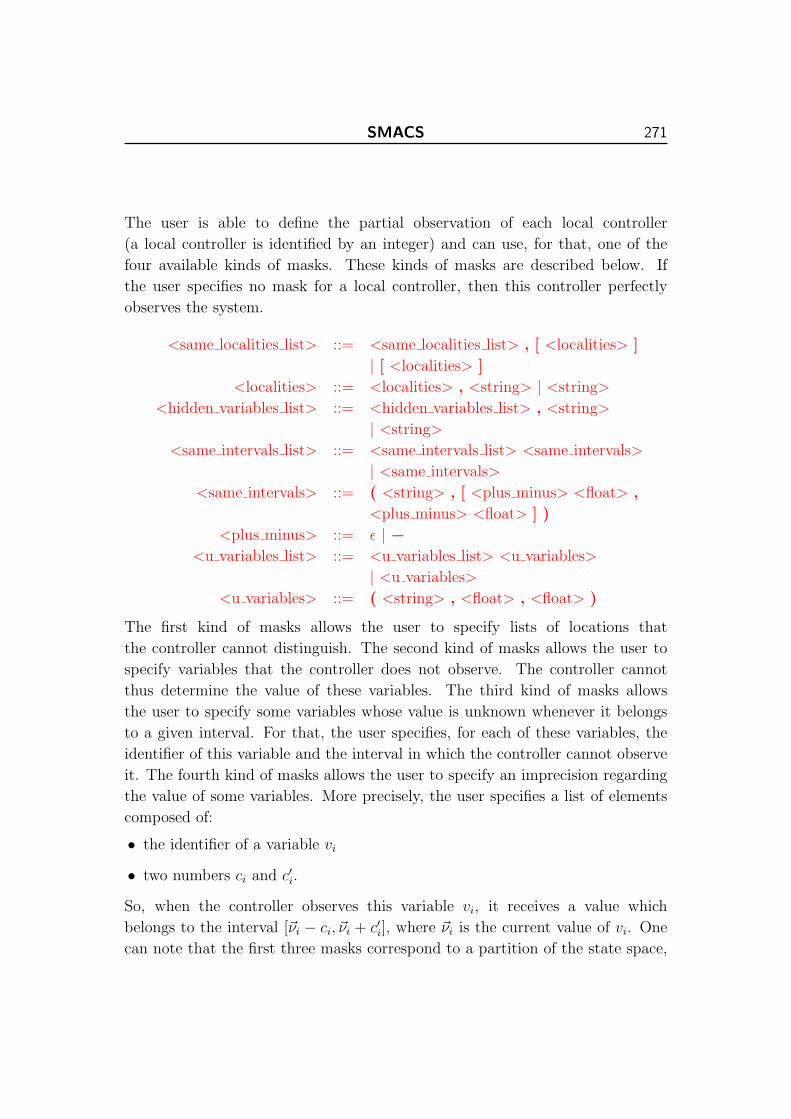
SMACS 271
The user is able to define the partial observation of each local controller
(a local controller is identified by an integer) and can use, for that, one of the
four available kinds of masks. These kinds of masks are described below. If
the user specifies no mask for a local controller, then this controller perfectly
observes the system.
<same localities list> ::= <same localities list> , [ <localities> ]
| [ <localities> ]
<localities> ::= <localities> , <string> | <string>
<hidden variables list> ::= <hidden variables list> , <string>
| <string>
<same intervals list> ::= <same intervals list> <same intervals>
| <same intervals>
<same intervals> ::= ( <string> , [ <plus minus> <float> ,
<plus minus> <float> ] )
<plus minus> ::= ε | −<u variables list> ::= <u variables list> <u variables>
| <u variables>
<u variables> ::= ( <string> , <float> , <float> )
The first kind of masks allows the user to specify lists of locations that
the controller cannot distinguish. The second kind of masks allows the user to
specify variables that the controller does not observe. The controller cannot
thus determine the value of these variables. The third kind of masks allows
the user to specify some variables whose value is unknown whenever it belongs
to a given interval. For that, the user specifies, for each of these variables, the
identifier of this variable and the interval in which the controller cannot observe
it. The fourth kind of masks allows the user to specify an imprecision regarding
the value of some variables. More precisely, the user specifies a list of elements
composed of:
• the identifier of a variable vi
• two numbers ci and c′i.
So, when the controller observes this variable vi, it receives a value which
belongs to the interval [~νi − ci, ~νi + c′i], where ~νi is the current value of vi. One
can note that the first three masks correspond to a partition of the state space,
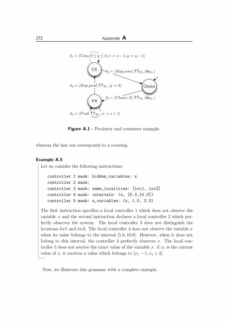
272 Appendix A
δ4 = 〈Stop prod;TTDV ; y := 2〉
δ2 = 〈Stop cons;TTDV ; IdDV 〉
δ3 = 〈Prod;TTDV ;x := x + 1〉
δ1 = 〈Cons; 0 ≤ y ≤ 2;x := x− 1, y := y − 1〉
δ9 = 〈Choice X;TTDV ; IdDV 〉
CX
PX
Choice
Figure A.1 - Producer and consumer example.
whereas the last one corresponds to a covering.
Example A.5
Let us consider the following instructions:
controller 1 mask: hidden_variables: x
controller 2 mask:
controller 3 mask: same_localities: [loc1, loc2]
controller 4 mask: intervals: (x, [5.0,10.0])
controller 5 mask: u_variables: (x, 1.0, 2.0)
The first instruction specifies a local controller 1 which does not observe the
variable x and the second instruction declares a local controller 2 which per-
fectly observes the system. The local controller 3 does not distinguish the
locations loc1 and loc2. The local controller 4 does not observe the variable x
when its value belongs to the interval [5.0, 10.0]. However, when it does not
belong to this interval, the controller 4 perfectly observes x. The local con-
troller 5 does not receive the exact value of the variable x: if x1 is the current
value of x, it receives a value which belongs to [x1 − 1, x1 + 2].
Now, we illustrate this grammar with a complete example.
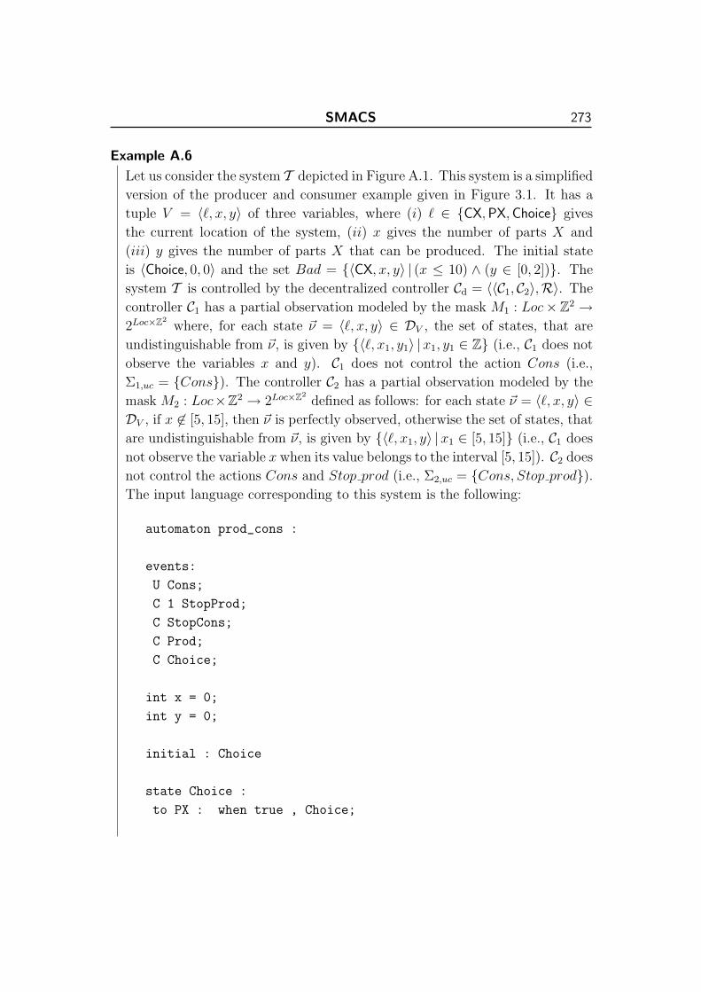
SMACS 273
Example A.6
Let us consider the system T depicted in Figure A.1. This system is a simplified
version of the producer and consumer example given in Figure 3.1. It has a
tuple V = 〈`, x, y〉 of three variables, where (i) ` ∈ {CX,PX,Choice} gives
the current location of the system, (ii) x gives the number of parts X and
(iii) y gives the number of parts X that can be produced. The initial state
is 〈Choice, 0, 0〉 and the set Bad = {〈CX, x, y〉 | (x ≤ 10) ∧ (y ∈ [0, 2])}. The
system T is controlled by the decentralized controller Cd = 〈〈C1, C2〉,R〉. The
controller C1 has a partial observation modeled by the mask M1 : Loc× Z2 →2Loc×Z2
where, for each state ~ν = 〈`, x, y〉 ∈ DV , the set of states, that are
undistinguishable from ~ν, is given by {〈`, x1, y1〉 |x1, y1 ∈ Z} (i.e., C1 does not
observe the variables x and y). C1 does not control the action Cons (i.e.,
Σ1,uc = {Cons}). The controller C2 has a partial observation modeled by the
mask M2 : Loc×Z2 → 2Loc×Z2defined as follows: for each state ~ν = 〈`, x, y〉 ∈
DV , if x 6∈ [5, 15], then ~ν is perfectly observed, otherwise the set of states, that
are undistinguishable from ~ν, is given by {〈`, x1, y〉 |x1 ∈ [5, 15]} (i.e., C1 does
not observe the variable x when its value belongs to the interval [5, 15]). C2 does
not control the actions Cons and Stop prod (i.e., Σ2,uc = {Cons, Stop prod}).The input language corresponding to this system is the following:
automaton prod_cons :
events:
U Cons;
C 1 StopProd;
C StopCons;
C Prod;
C Choice;
int x = 0;
int y = 0;
initial : Choice
state Choice :
to PX : when true , Choice;

274 Appendix A
state PX:
to PX : when true , Prod with x = x + 1;
to CX : when true , StopProd with y = 2;
state CX:
to CX : when y <= 2 and y >= 0 , Cons with x = x - 1,
y = y - 1;
to Choice : when true , StopCons;
bad_states:
state CX : x <= 10 and y <= 2 and y >= 0
controller 0 mask: hidden_variables: x, y
controller 1 mask: intervals: (x, [5.0, 15.0])
Input Options. SMACS is called by the command bin/smacs.byte. The main
options offered to the user are:
• -non-blocking : ensures that the controlled system is deadlock-free.
• -dot-output <string>: gives the name of the dot file in which the controlled
system is saved. By default, the dot file is not generated.
• -text-output <string>: gives the name of the text file in which the controlled
system is saved. The format used in this text file to describe the controlled
system is very close to the one used in the input language to describe the
system to be controlled. By default, this file is not generated.
• -widening-start <integer>: gives the iteration at which the widening operator
is used for the first time in the fixpoint computation (by default, it is 2).
• -widening-freq <integer>: gives the number of iterations (in the fixpoint com-
putation) between two successive applications of the widening operator (by
default, it is 1).
• -descending-steps <integer>: gives the number of descending steps i.e., the
number of additional iterations to be performed in the fixpoint computation
to refine the computed post-fixpoint (by default, it is 2).
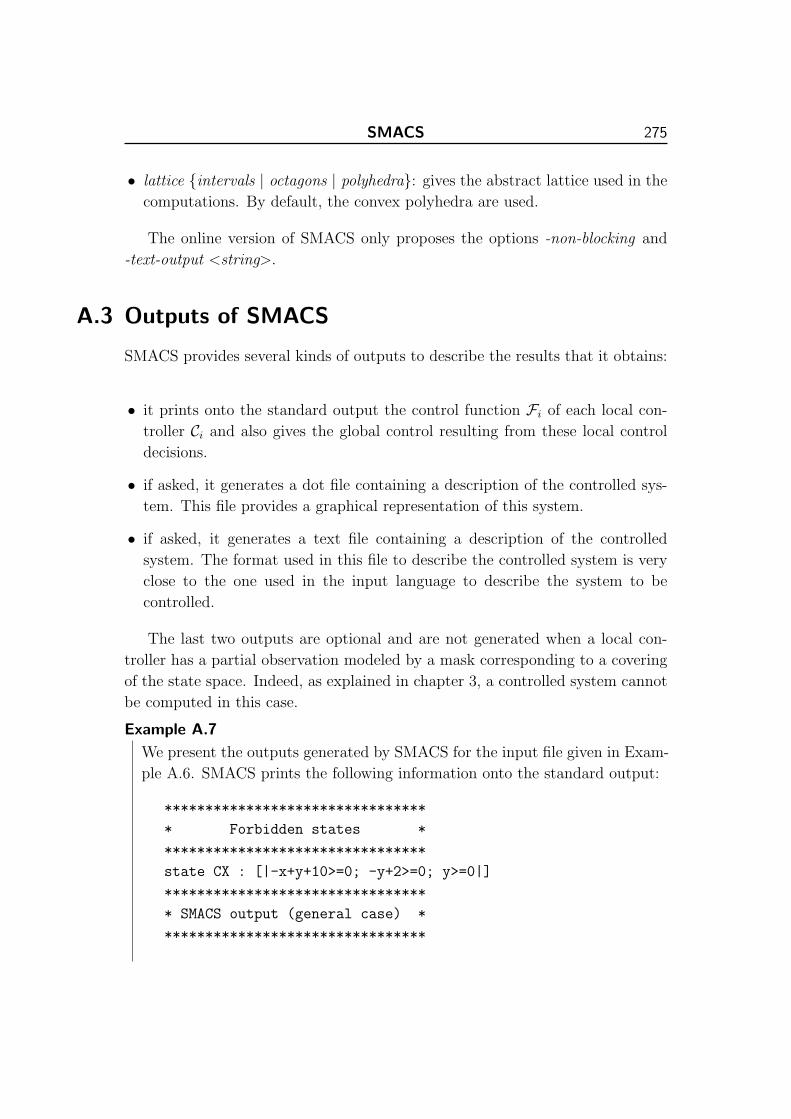
SMACS 275
• lattice {intervals | octagons | polyhedra}: gives the abstract lattice used in the
computations. By default, the convex polyhedra are used.
The online version of SMACS only proposes the options -non-blocking and
-text-output <string>.
A.3 Outputs of SMACS
SMACS provides several kinds of outputs to describe the results that it obtains:
• it prints onto the standard output the control function Fi of each local con-
troller Ci and also gives the global control resulting from these local control
decisions.
• if asked, it generates a dot file containing a description of the controlled sys-
tem. This file provides a graphical representation of this system.
• if asked, it generates a text file containing a description of the controlled
system. The format used in this file to describe the controlled system is very
close to the one used in the input language to describe the system to be
controlled.
The last two outputs are optional and are not generated when a local con-
troller has a partial observation modeled by a mask corresponding to a covering
of the state space. Indeed, as explained in chapter 3, a controlled system cannot
be computed in this case.
Example A.7
We present the outputs generated by SMACS for the input file given in Exam-
ple A.6. SMACS prints the following information onto the standard output:
********************************
* Forbidden states *
********************************
state CX : [|-x+y+10>=0; -y+2>=0; y>=0|]
********************************
* SMACS output (general case) *
********************************
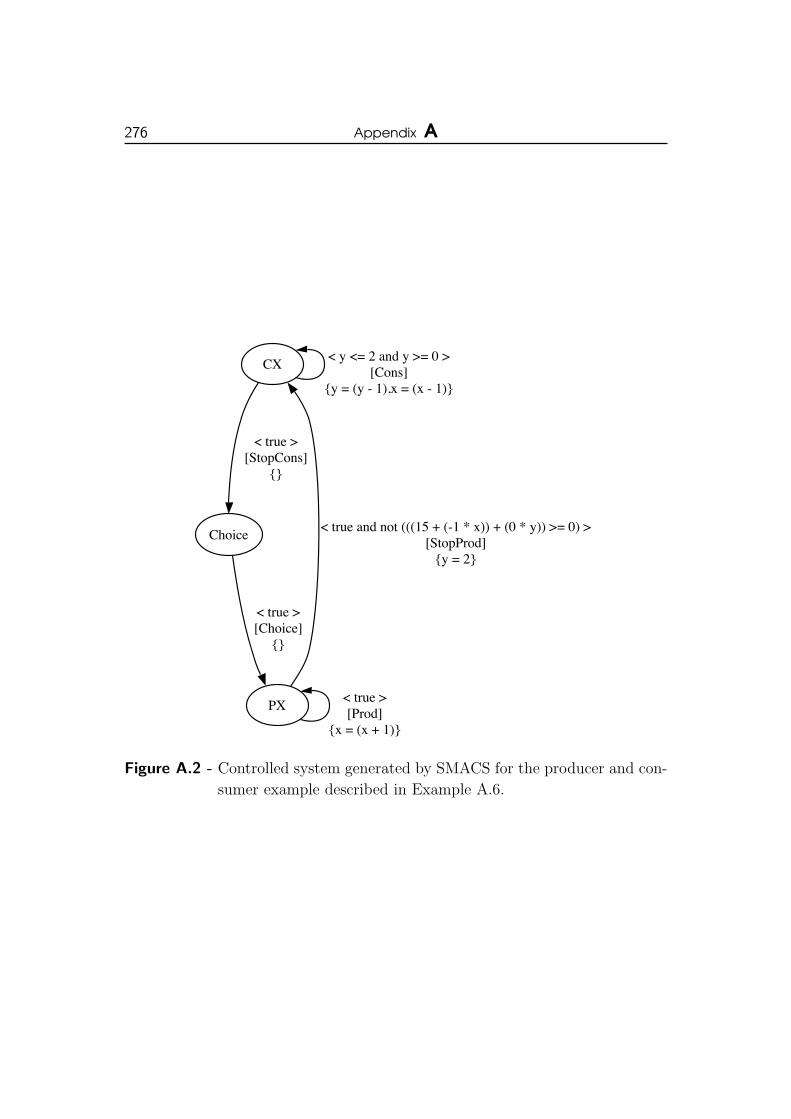
276 Appendix A
CX
< y <= 2 and y >= 0 >
[Cons]{y = (y - 1),x = (x - 1)}
Choice
< true >
[StopCons]{}
PX
< true and not (((15 + (-1 * x)) + (0 * y)) >= 0) >
[StopProd]{y = 2}
< true >
[Prod]{x = (x + 1)}
< true > [Choice]
{}
Figure A.2 - Controlled system generated by SMACS for the producer and con-
sumer example described in Example A.6.

SMACS 277
---------------------
Controller 1 function
---------------------
disable event StopProd in state PX when [|-x+15>=0|]
---------------------
Controller 0 function
---------------------
-----------------------
Global control function
-----------------------
disable event StopProd in state PX when [|-x+15>=0|]
Thus, the set of forbidden states I(Bad) = {〈`, x, y〉 | (x− y ≤ 10) ∧ (0 ≤ y ≤2)}. The local controller 1 forbids the action Stop prod in the location PX
when x ≤ 15 and the local controller 2 forbids no action. The resulting global
control consists in forbidding the action Stop prod in the location PX when
x ≤ 15.
The information written in the dot file gives the controlled system depicted in
Figure A.2.
The description of the controlled system written in the text file is the following:
Automaton controlled_prod-cons :
events:
C Choice,
C Prod,
C StopCons,
C 1 StopProd,
U Cons
int y;
int x;

278 Appendix A
initial condition: Choice => x == 0 and y == 0
state CX :
to Choice : when true, StopCons;
to CX : when y <= 2 and y >= 0, Cons with y = (y - 1),
x = (x - 1);
state PX :
to CX : when not (((15 + (-1 * x)) + (0 * y)) >= 0), StopProd
with y = 2;
to PX : when true, Prod with x = (x + 1);
state Choice :
to PX : when true, Choice;
Bibliography
[ACH+95] R. Alur, C. Courcoubetis, N. Halbwachs, T. A. Henzinger, P.-H. Ho,
X. Nicollin, A. Olivero, J. Sifakis, and S. Yovine. The algorithmic
analysis of hybrid systems. Theor. Comput. Sci., 138(1):3–34, 1995.
[AD90] R. Alur and D.L. Dill. Automata for modeling real-time systems.
In Proceedings of the seventeenth international colloquium on Au-
tomata, languages and programming, pages 322–335, New York,
USA, 1990. Springer-Verlag New York, Inc.
[AD94] R. Alur and D.L. Dill. A theory of timed automata. Theoretical
Computer Science, 126(2):183–235, 1994.
[AMP95] E. Asarin, O. Maler, and A. Pnueli. Symbolic controller synthesis
for discrete and timed systems. Lecture Notes in Computer Science,
999:1–20, 1995.
[AMPS98] E. Asarin, O. Maler, A. Pnueli, and J. Sifakis. Controller synthesis
for timed automata. In Proceedings of the 5th IFAC Cconference
on System Structure and Control (SSC’98), pages 469–474. Elsevier
Science, July 1998.
[AP68] R. Aron and V. Pareto. Traite de sociologie generale. Droz, 1968.
[ASU86] Alfred V. Aho, Ravi Sethi, and Jeffrey D. Ullman. Compilers: prin-
ciples, techniques, and tools. Addison-Wesley Longman Publishing
Co., Inc., Boston, MA, USA, 1986.
[BDMP03] P. Bouyer, D. D’Souza, P. Madhusudan, and A. Petit. Timed con-
trol with partial observability. In Warren A. Hunt, Jr and Fabio
Somenzi, editors, Proceedings of the 15th International Conference
on Computer Aided Verification (CAV’03), volume 2725 of Lecture
Notes in Computer Science, pages 180–192. Springer, July 2003.
279

280 Bibliography
[BGWW97] Bernard Boigelot, Patrice Godefroid, Bernard Willems, and Pierre
Wolper. The power of qdds. In SAS ’97: Proceedings of the 4th In-
ternational Symposium on Static Analysis, pages 172–186, London,
UK, 1997. Springer-Verlag.
[BL98] G. Barrett and S. Lafortune. A novel framework for decentralized
supervisory control with communication. In IEEE Conference on
Systems, Man, and Cybernetics, pages 11–14, San Diego, California,
October 1998.
[BL00] G. Barrett and S. Lafortune. Decentralized supervisory control with
communicating controllers. IEEE Transactions on Automatic Con-
trol, 45(9):1620–1638, 2000.
[Bou92] F. Bourdoncle. Semantiques des Langages Imperatifs d’Ordre
Superieur et Interpretation Abstraite. PhD thesis, Ecole Polytech-
nique, 1992.
[BZ83a] D. Brand and P. Zafiropulo. On communicating finite-state ma-
chines. Journal of the ACM, 30(2):323–342, 1983.
[BZ83b] Daniel Brand and Pitro Zafiropulo. On communicating finite-state
machines. J. ACM, 30(2):323–342, 1983.
[Cama] The CamlIDL Library. Available http://caml.inria.fr/pub/
old caml site/camlidl/. [August 12, 2010].
[Camb] The Camllib Library. Available http://pop-art.inrialpes.fr/∼bjeannet/bjeannet-forge/camllib/index.html. [August 12,
2010].
[CC77] P. Cousot and R. Cousot. Abstract interpretation: a unified lattice
model for static analysis of programs by construction or approxima-
tion of fixpoints. In POPL’77, pages 238–252, 1977.
[CDF+05] F. Cassez, A. David, E. Fleury, K.G. Larsen, and D. Lime. Efficient
on-the-fly algorithms for the analysis of timed games. CONCUR
2005 - Concurrency Theory, pages 66–80, 2005.
[CDHR07] K. Chatterjee, L. Doyen, T. A. Henzinger, and J.-F. Raskin. Algo-
rithms for omega-regular games of incomplete information. Logical
Methods in Computer Science, 3(3:4), 2007.

Bibliography 281
[CE82] E. M. Clarke and E. A. Emerson. Design and synthesis of synchro-
nization skeletons using branching-time temporal logic. In Logic
of Programs, Workshop, pages 52–71, London, UK, 1982. Springer-
Verlag.
[CH78] P. Cousot and N. Halbwachs. Automatic discovery of linear re-
straints among variables of a program. In POPL ’78, pages 84–96,
1978.
[Chu36] A. Church. An unsolvable problem of elementary number theory.
American Journal of Mathematics, 58:345–363, 1936.
[CL08] C. Cassandras and S. Lafortune. Introduction to Discrete Event
Systems (2nd edition). Springer, 2008.
[Cou81] P. Cousot. Semantic foundations of program analysis. In S.S. Much-
nick and N.D. Jones, editors, Program Flow Analysis: Theory and
Applications, chapter 10, pages 303–342. Prentice-Hall, Inc., Engle-
wood Cliffs, New Jersey, 1981.
[Dar05] P. Darondeau. Distributed implementations of Ramadge-Wonham
supervisory control with petri nets. In 44th IEEE Conference on De-
cision and Control and European Control Conference, pages 2107–
2112, Sevilla, Spain, December 2005.
[DDR06] M. De Wulf, L. Doyen, and J.-F. Raskin. A lattice theory for solving
games of imperfect information. In J.P. Hespanha and A. Tiwari,
editors, HSCC, volume 3927 of Lecture Notes in Computer Science,
pages 153–168. Springer, 2006.
[DM02] D. D’Souza and P. Madhusudan. Timed control synthesis for exter-
nal specifications. In STACS ’02: Proceedings of the 19th Annual
Symposium on Theoretical Aspects of Computer Science, pages 571–
582. Springer-Verlag, 2002.
[DRS01] N. Dor, M. Rodeh, and S. Sagiv. Cleanness checking of string ma-
nipulations in c programs via integer analysis. In SAS ’01: Proceed-
ings of the 8th International Symposium on Static Analysis, pages
194–212, London, UK, 2001. Springer-Verlag.
282 Bibliography
[Dub06] J. Dubreil. Non-interference on symbolic transition system. Tech-
nical report, Uppsala University, February 2006.
[Fix09] Fixpoint: an OCaml library implementing a generic fix-point en-
gine, 2009. Available http://pop-art.inrialpes.fr/people/
bjeannet/bjeannet-forge/fixpoint/. [August 12, 2010].
[GD07] B. Gaudin and P.H. Deussen. Supervisory control on concurrent dis-
crete event systems with variables. In American Control Conference
2007, July 2007.
[GJ90] M. R. Garey and D. S. Johnson. Computers and Intractability: A
Guide to the Theory of NP-Completeness. W. H. Freeman & Co.,
New York, NY, USA, 1990.
[GM05] B. Gaudin and H. Marchand. Efficient computation of supervisors
for loosely synchronous discrete event systems: A state-based ap-
proach. In 6th IFAC World Congress, Prague, Czech Republic, July
2005.
[GMP] The GMP library. Available http://gmplib.org/. [August 12,
2010].
[God96] P. Godefroid. Partial-Order Methods for the Verification of Con-
current Systems: An Approach to the State-Explosion Problem.
Springer-Verlag New York, Inc., 1996.
[HB91] C. Hoaxum and H. Baosheng. Distributed control of discrete event
systems described by a class of controlled petri nets. In Preprints of
IFAC International Symposium on Distributed Intelligence Systems,
Virginia, 1991.
[HHWt97] T. A. Henzinger, P-H. Ho, and H. Wong-toi. Hytech: A model
checker for hybrid systems. Software Tools for Technology Transfer,
1:460–463, 1997.
[HK99] T.A. Henzinger and P.W. Kopke. Discrete-time control for rectangu-
lar hybrid automata. Theoretical Computer Science, 221(1-2):369–
392, 1999.

Bibliography 283
[HKG97] L.E. Holloway, B.H. Krogh, and A. Giua. A survey of Petri net
methods for controlled discrete event systems. Discrete Event Dy-
namic Systems: Theory and Application, 7:151–190, 1997.
[HMR05] T.A. Henzinger, R. Majumdar, and J.-F. Raskin. A classification of
symbolic transition systems. ACM Trans. Comput. Logic, 6(1):1–32,
2005.
[HMU06] J. E. Hopcroft, R. Motwani, and J. D. Ullman. Introduction
to Automata Theory, Languages, and Computation (3rd Edition).
Addison-Wesley Longman Publishing Co., Inc., Boston, MA, USA,
2006.
[Hol04] G. J. Holzmann. The SPIN Model Checker : Primer and Reference
Manual. Addison-Wesley Professional, 2004.
[HPR97] N. Halbwachs, Y.E. Proy, and P. Roumanoff. Verification of real-
time systems using linear relation analysis. Formal Methods in Sys-
tem Design, 11(2):157–185, August 1997.
[HTL08] R.C. Hill, D.M. Tilbury, and S. Lafortune. Covering-based super-
visory control of partially observed discrete event systems for state
avoidance. In 9th International Workshop on Discrete Event Sys-
tems, May 2008.
[Jea03] B. Jeannet. Dynamic partitioning in linear relation analysis. Appli-
cation to the verification of reactive systems. Formal Meth. in Syst.
Design, 23(1):5–37, 2003.
[JM09] B. Jeannet and A. Mine. The APRON library, 2009. Available
http://apron.cri.ensmp.fr/. [August 12, 2010].
[JMR06] T. Jeron, H. Marchand, and V. Rusu. Symbolic determinisation
of extended automata. In 4th IFIP International Conference on
Theoretical Computer Science, Santiago, Chili, August 2006.
[KG05] R. Kumar and V.K. Garg. On computation of state avoidance con-
trol for infinite state systems in assignment program model. IEEE
Trans. on Autom. Science and Engineering, 2(2):87–91, 2005.
284 Bibliography
[KGM91] R. Kumar, V. Garg, and S. I. Marcus. On controllability and nor-
mality of discrete event dynamical systems. Systems and Control
Letters, 17:17–157, 1991.
[KGM93] R. Kumar, V. Garg, and S.I. Marcus. Predicates and predicate
transformers for supervisory control of discrete event dynamical sys-
tems. IEEE Trans. Autom. Control, 38(2):232–247, 1993.
[KH90] B. H. Krogh and L. E. Holloway. Synthesis of feedback control
logic for a class of controlled petri nets. IEEE Trans. on Automatic
Control, 35(5):514–523, 1990.
[KH91] B. H. Krogh and L. E. Holloway. Synthesis of feedback control
logic for discrete manufacturing systems. International Federation
Of Automatic Control, 27(4):641–651, 1991.
[KH92] B. H. Krogh and L. E. Holloway. On closed-loop liveness of discrete
event systems under maximally permissive control. IEEE Trans. on
Automatic Control, 37(5):692–697, 1992.
[KH96] R. Kumar and L.E. Holloway. Supervisory control of deterministic
petri nets with regular specification languages. IEEE Trans. on
Automatic Control, 41(2):245–249, 1996.
[KL10] G. Kalyon and T. Le Gall. The SMACS Tool, 2010. Available
http://www.smacs.be/ [August 12, 2010].
[KLMM10] G. Kalyon, T. Le Gall, H. Marchand, and T. Massart. Decentralized
control of infinite systems. submitted to Journal of Discrete Event
Dynamical Systems, 2010.
[Kna28] B. Knaster. Un theoreme sur les fonctions densembles. Annales de
la Societe Polonaise de Mathematique, 6:194–212, 1928.
[Kri63] S.A. Kripke. Semantical consideration on modal logic. Acta Phili-
sophica Fennica, 16:83–94, 1963.
[Kro87] B.H. Krogh. Controlled petri nets and maximally permissive feed-
bak logic. In Proc. of the 25th Annual Allerton Conf., Univeristy of
Illinois, Urbana., 1987.

Bibliography 285
[Lam78] L. Lamport. Time, clocks, and the ordering of events in a distributed
system. Communications of the ACM, 21(7):558–565, 1978.
[LGJJ06] T. Le Gall, B. Jeannet, and T. Jeron. Verification of communication
protocols using abstract interpretation of fifo queues. In Michael
Johnson and Varmo Vene, editors, 11th International Conference
on Algebraic Methodology and Software Technology, AMAST ’06,
Kuressaare, Estonia, LNCS. Springer-Verlag, July 2006.
[LJM05] T. Le Gall, B. Jeannet, and H. Marchand. Supervisory control
of infinite symbolic systems using abstract interpretation. In CD-
C/ECC’05, December 2005.
[Lov78] D.W. Loveland. Automated theorem proving: A logical basis (Funda-
mental studies in computer science). Elsevier North-Holland, 1978.
[LW88] F. Lin and W.M. Wonham. On observability of discrete-event sys-
tems. Inf. Sci., 44(3):173–198, 1988.
[Mar97] J. C. Martin. Introduction to Languages and the Theory of Compu-
tation. McGraw-Hill Higher Education, 1997.
[Mat89] F. Mattern. Virtual time and global states of distributed systems. In
Proceedings of the Workshop on Parallel and Distributed Algorithms,
pages 215–226, North-Holland / Elsevier, 1989.
[McM93] K. L. McMillan. Symbolic Model Checking. Kluwer Academic Pub-
lishers., 1993.
[Min01] A. Mine. The octagon abstract domain. In Proceedings of the Work-
shop on Analysis, Slicing, and Transformation (AST’01), IEEE,
pages 310–319, Stuttgart, Gernamy, October 2001. IEEE CS Press.
[MLG] The MLGMPIDL Library. Available http://www.inrialpes.fr/
pop-art/people/bjeannet/mlxxxidl-forge/mlgmpidl/. [August
12, 2010].
[MPF] The MPFR library. Available http://www.mpfr.org/. [August 12,
2010].
286 Bibliography
[MPS95] O. Maler, A. Pnueli, and J. Sifakis. On the synthesis of discrete
controllers for timed systems (an extended abstract). In Ernst W.
Mayr and Claude Puech, editors, Proceedings of the 12th Symposium
on Theoretical Aspects of Computer Science (STACS’95), volume
900 of Lecture Notes in Computer Science, pages 229–242. Springer-
Verlag, March 1995.
[Mye79] G. J. Myers. Art of Software Testing. John Wiley & Sons, Inc.,
New York, NY, USA, 1979.
[OCa09] The programming language Objective CAML, 2009. Available
http://caml.inria.fr/. [August 12, 2010].
[Pap94] C. M. Papadimitriou. Computational complexity. Addison-Wesley,
Reading, Massachusetts, 1994.
[Pet62] C.A. Petri. Kommunikation mit automaten. Rheinisch-Westfaliches
Institut fur Intrumentelle Mathematik an der Universitat Bonn,
Schrift Nr 2, 1962.
[Pnu77] A. Pnueli. The temporal logic of programs. In Proceedings of
the 18th Annual Symposium on Foundations of Computer Science
(FOCS), pages 46–57, 1977.
[PR89] A. Pnueli and R. Rosner. On the synthesis of an asynchronous reac-
tive module. In G. Ausiello, M. Dezani-Ciancaglini, and S.R. Della
Rocca, editors, ICALP, volume 372 of Lecture Notes in Computer
Science, pages 652–671. Springer, 1989.
[PVK01] D. Peled, A. Valmari, and I. Kokkarinen. Relaxed visibility en-
hances partial order reduction. Formal Methods in System Design,
19(3):275–289, 2001.
[QS82] J.-P. Queille and J. Sifakis. Specification and verification of con-
current systems in cesar. In Proceedings of the 5th Colloquium on
International Symposium on Programming, pages 337–351, London,
UK, 1982. Springer-Verlag.
[RDFV88] Cieslak R., C. Desclaux, A. Fawaz, and P. Varaiya. Supervisory
control of discrete-event process with partial observation. IEEE
Trans. on Automatic Control, 33(3):249–260, 1988.

Bibliography 287
[Rei84] J.H. Reif. The complexity of two-player games of incomplete infor-
mation. J. Comput. Syst. Sci., 29(2):274–301, 1984.
[Ric03] K. Ricker, S.L. Rudie. Knowledge is a terrible thing to waste: using
inference in discrete-event control problems. In ACC’03: Proceed-
ings of the 2003 conference on American Control Conference, pages
2246—2251, 2003.
[RP05] S. Riedweg and S. Pinchinat. You can always compute maximally
permissive controllers under partial observation when they exist. In
Proc. 2005 American Control Conference., volume 4, pages 2287–
2292, Portland, Oregon, jun 2005.
[RW87] P.J. Ramadge and W.M. Wonham. Modular feedback logic for dis-
crete event systems. SIAM J. Control Optim., 25(5):1202–1218,
September 1987.
[RW89] P.J. Ramadge and W.M. Wonham. The control of discrete event
systems. Proceedings of the IEEE; Special issue on Dynamics of
Discrete Event Systems, 77(1):81–98, 1989.
[RW92a] K. Rudie and W. M. Wonham. An automata-theoretic approach to
automatic program verification. In Proceedings of the IEEE Con-
ference on Decision and Control (CDC), pages 3770–3777, Tucson,
Arizona, 1992.
[RW92b] K. Rudie and W. M. Wonham. Think globally, act locally: de-
centralized supervisory control. IEEE Transactions on Automatic
Control, 37(11):1692–1708, November 1992.
[RW95] K. Rudie and J. C. Willems. The computational complexity of
decentralized discrete-event control problems. IEEE Transactions
on Automatic Control, 40:1313–1319, 1995.
[SAF09] M. Skoldstam, K. Akesson, and F. Fabian. Supervisory control
applied to automata extended with variables. Technical Report
R001/2008, Department of Signals and Systems, Chalmers Univer-
sity of Technology, Goteborg, Sweden,, 2009.

288 Bibliography
[Sre93] R. S. Sreenivas. On a weaker notion of controllability of a language k
with respect to to a language l. IEEE Trans. on Automatic Control,
38(9):1446–1447, 1993.
[Tar55] A. Tarski. A lattice-theoretical fixpoint theorem and its applica-
tions. Pacific Journal of Mathematics, 5:285–309, 1955.
[Thi05] J. G. Thistle. Undecidability in decentralized supervision. Systems
& Control Letters, 54(5):503–509, 2005.
[TK97] S. Takai and S. Kodama. M-controllable subpredicates arising in
state feedback control of discrete event systems. International Jour-
nal of Control, 67(4):553–566, 1997.
[TK98] S. Takai and S. Kodama. Characterization of all m-controllable
subpredicates of a given predicate. International Journal of Control,
70:541–549(9), 10 July 1998.
[TKU94] Shigemasa Takai, Shinzo Kodama, and Toshimitsu Ushio. Decen-
tralized state feedback control of discrete event systems. Syst. Con-
trol Lett., 22(5):369–375, 1994.
[Tri02] Stavros Tripakis. Decentralized control of discrete event systems
with bounded or unbounded delay communication. In WODES ’02.
IEEE Computer Society, 2002.
[Tsi89] J. N. Tsitsiklis. On the control of discrete event dynamical systems.
Mathematics of Control, Signals and Systems, 2(2):95–107, 1989.
[TUK95] S. Takai, T. Ushio, and S. Kodama. Static-state feedback control of
discrete-event systems under partial observation. IEEE transactions
on automatic control, 40:1950–1954(11), 11 November 1995.
[Ush89] T. Ushio. On controllable predicates and languages in discrete-event
systems. In Proc. of the 28th Conference on Decision and Control,
pages 123–124, Tampa, Floride, Decembre 1989.
[VNJ90] N. Viswanadham, Y. Narahari, and T.L. Johnson. Deadlock preven-
tion and deadlock avoidance in flexible manufacturing systems using
petri net models. IEEE Transactions on Robotics and Automation,
6(6):713–723, 1990.
Bibliography 289
[VW86] M.Y. Vardi and P. Wolper. An automata-theoretic approach to
automatic program verification. In Proc. 1st Symp. on Logic in
Computer Science, pages 332–344, June 1986.
[Won05] W.M. Wonham. Lecture notes on control of discrete-event systems.
Technical report, University of Toronto, 2005.
[WR87] W. Wonham and P. Ramadge. On the supremal controllable sub-
language of a given language. SIAM Journal on Control and Opti-
mization, 25(3):637–659, 1987.
[XK09] S. Xu and R. Kumar. Distributed state estimation in discrete event
systems. In ACC’09: Proceedings of the 2009 conference on Amer-
ican Control Conference, pages 4735–4740. IEEE Press, 2009.
[YL02] T.-S. Yoo and S. Lafortune. A general architecture for decentral-
ized supervisory control of discrete-event systems. Discrete Event
Dynamic Systems, 12(3):335–377, 2002.
[YL04] T.-S. Yoo and S. Lafortune. Decentralized supervisory control with
conditional decisions: supervisor existence. IEEE Transactions on
Automatic Control, 49(11):1886–1904, 2004.

290 Bibliography