supply chain design under risk management constraints · pdf filesupply chain design under...
TRANSCRIPT

Supply Chain Design Under Risk Management Constraints
Jenny Leung Javaneh Zavari
A thesis submitted in partial fulfillment of the requirements for the degree of
BACHELOR OF APPLIED SCIENCE
Supervisor: Professor Roy Kwon
Department of Mechanical and Industrial Engineering University of Toronto
March 2007

ii
ABSTRACT
Having a strong supply chain network which ensures that supply is equal to expected demand is crucial to ensure a successful and profitable company. Two areas of focus within this thesis is location strategy for distribution centres and the effective distribution of products. This thesis will investigate the weaknesses of the existing models that currently address these issues and will provide improvements to develop a model that will best satisfy the problem on hand. The model in this thesis is a 2-stage stochastic programming model that will integrate the existing maximal covering location model with an asset–liability structure. This thesis evaluates the benefits of the stochastic model by comparing the results to those of existing models through the use of a hypothetical case. Upon solving, it is evident that the stochastic model is superior in terms of cost minimization when demand uncertainty is involved.
iii
ACKNOWLEDGEMENTS
We would like to give our outmost appreciation and sincere thanks to our thesis
supervisor Professor R. Kwon, for his support, advice and guidance during the
course of this project. Without his support, this project would not have been a
success.
We would also like to thank Jenny Leung and Javaneh Zavari for their hard work.
Lastly, we like to thank our families for giving us moral support and guidance
iv
LIST OF SYMBOLS
Xj= Locating facility at j
Zi= Demand coverage of facility at i
Di= Average demand at point i
P = # of distribution centres allowable
Ci=Cost of locating distribution centre i
h=Unit price of product
Tij= Cost of transporting one unit of product from distribution centre i to demand
point j
Xi = Location decision for distribution centre i
Yij= Amount of demand satisfied at demand point j by distribution centre i
n= number of demand points
m= number of scenarios
Lj= Capacity available at location j
Djs= Amount of demand at point j under scenario s
Yijs= Amount of demand satisfied at demand point j by distribution centre i under
scenario s
Ps= Probability of scenario s occurring

v
LIST OF FIGURES
Figure 1.1 - Supply chain example for automobile company…………………………..2 Figure 4.1 - Demand Network for Maximal Covering Location Model……..………...12 Figure 4.2 - Lingo Model for Maximal Covering Location Model……………………..14 Figure 4.3 - Lingo Solution for Maximal Covering Location Model…………………...15

vi
LIST OF TABLES
TABLE 4.1 - Data for Farmer’s Problem TABLE 4.2 - Optimal solution based on expected yields in Farmer’s Problem TABLE 4.3 - Optimal solution based on above average yields (+20%) in Farmer’s Problem TABLE 4.4 - Optimal solution based on below average yields (-20%) in Farmer’s Problem TABLE 4.5 - Optimal solution for the stochastic model (1.2) TABLE 6.1 - Amount of demand at each point for each scenario for case TABLE 6.2 - Transportation costs to move one unit of product between points for case TABLE 6.3 - Cost of locating a distribution centre for case TABLE 7.1 - Cost comparison of scenarios in case TABLE 7.2 - Demand values of 3 scenarios in case TABLE 7.3 - Demand values of scenarios of difference variance in case TABLE7.4 - Costs for variance scenarios A, B, and C for models in case

TABLE OF CONTENTS
LIST OF SYMBOLS……………………………………………………………………………………….iv LIST OF FIGURES…………………………………………………………………………………………v LIST OF TABLES……………………………………………………………………………………….…vi 1. INTRODUCTION ................................................................................................................... 1 2. PROBLEM ............................................................................................................................. 3 3. OBJECTIVE ........................................................................................................................... 4 4. LITERATURE REVIEW ......................................................................................................... 6
4.1 FINANCIAL PLANNING MODEL ...................................................................... 6 4.1.1 Why a multi-period framework? ........................................................................ 6 4.1.2 Financial Planning vs. Facility Planning ............................................................ 8
4.2 CURRENT MODEL ......................................................................................... 10 4.2.1 Maximal Covering Location Model .................................................................. 10 4.2.2 Weaknesses of Current Models ...................................................................... 15 4.2.3 The Farmer’s Problem .................................................................................... 17
4.2.3.1 Deterministic Model for Farmer’s Problem ................................. 17 4.2.3.2 A Scenario Representation......................................................... 19 4.2.3.3 Stochastic Model for Farmer’s Problem ..................................... 20 4.2.3.4 General model formulation ......................................................... 23
5. SUPPLY CHAIN DESIGN FOR DISTRIBUTION CENTRES .............................................. 25 5.1 DETERMINISTIC MODEL FORMULATION (MODEL 1) ................................ 25 5.2 STOCHASTIC MODEL FORMULATION (MODEL 3)..................................... 27
6. APPLICATION OF MODEL ................................................................................................. 29 6.1 DATA ............................................................................................................... 29 6.2 DETERMINISTIC AND STOCHASTIC MODELS INCLUDING THE CASE ... 30
6.2.1 MODEL 1 ......................................................................................................... 30 6.2.2 MODEL 2 ......................................................................................................... 31 6.2.3 MODEL 3 ......................................................................................................... 34
7. RESULTS ............................................................................................................................ 38 7.1 SCENARIO COMPARISON OF MODEL 2 AND MODEL 3 ........................... 38 7.2 COMPARISON OF DIFFERENT DEGREES OF VARIANCE IN DEMAND ... 41
8. CONCLUSION ..................................................................................................................... 44 9. REFERENCES .................................................................................................................... 45 10. APPENDICES ...................................................................................................................... 46
APPENDIX A – DETERMINISTIC MODEL (MODEL 1) SOLUTION ............................... 46 APPENDIX B – DETERMINISTIC MODEL WITH STOCHASTIC STRUCTURE (MODEL 2) SOLUTION ................................................................................................................... 48 APPENDIX C – STOCHASTIC MODEL (MODEL 3) SOLUTION .................................... 51 APPENDIX D – MODEL FORMULATION AND SOLUTIONS FOR MODELS 2 AND 3 FOR SCENARIO 1 ........................................................................................................... 54 APPENDIX E – MODEL FORMULATION AND SOLUTIONS FOR MODELS 2 AND 3 FOR SCENARIO 2 ........................................................................................................... 59 APPENDIX F – MODEL FORMULATION AND SOLUTIONS FOR MODELS 2 AND 3 FOR SCENARIO 3 ........................................................................................................... 64 APPENDIX G – MODEL AND SOLUTIONS FOR DEMAND VARIANCE SCENARIO A (VARS1=8.54, VARS2=26.19, VARS3=69.40) ................................................................ 69 APPENDIX H – MODEL AND SOLUTIONS FOR DEMAND VARIANCE SCENARIO B (VARS1=6.02, VARS2=14.71, VARS3=21.75) ................................................................ 81 APPENDIX I – MODEL AND SOLUTIONS FOR DEMAND VARIANCE SCENARIO C (VARS1=3.30, VARS2=4.51, VARS3=12.31 ................................................................... 93 APPENDIX J – RESPONSIBILITIES OF GROUP MEMBERS ...................................... 105

1
1. INTRODUCTION
In the retail industry, the primary goal for all organizations is to satisfy their
customers. The factors affecting the failure or success of this objective depend
primarily on the decisions that the organization makes. A principle factor includes
the ability of the company to ensure that the supply of their products equals the
expected demand of the product from their customers while ensuring that costs are
minimized. In order to accomplish these goals, an important area of focus is
effective supply chain management.
SUPPLY CHIAN MANAGMENT
Supply chain management includes all facilities, activities, and information
associated with the flow and transformation of goods and services from the raw
material stage to the end user [1]. It also includes strategic network optimization
including the number, location, and size of warehouses, distribution centres, and
facilities [2]. An example of a simple automobile supply chain can be seen in Figure
1.1 [1].
Figure 1.1 – Supply chain example for automobile company
2
Location theory within the context of supply chain design aids in the decisions for the
optimal location of the organization’s assets (e.g. manufacturing facilities,
warehouses, distribution centres, etc.) which will ensure customer satisfaction while
minimizing overall costs
Based upon the initial decisions made by the company as to where to locate their
assets, the next decision is how to allocate the product in the most efficient manner
to meet the demand of a customer. Capacitated inventory models help in deciding
the level of stock to allocate to each distribution centre while considering the average
demand of the customer. Uncapacitated inventory models accomplish the same
task; however, they assume an infinite inventory stock level at all distribution
centres.
Some expenses that affect the organization’s decisions include cost of locating the
distribution centre, transportation costs, stock-out costs (deliver less than required
amount to demand points), penalties for delivering too much product to demand
points, and inventory costs (over-stocking costs).
3
2. PROBLEM
Failure in making optimal location and/or inventory decisions will ultimately result in
lost profit. There are many contributing factors towards sub-optimal decision-making,
but a key issue is supply chain uncertainty.
Currently the main problem is that the existing models that attempt to address supply
chain design issues, but do not take into account the uncertainty associated with
demand levels. As stated previously, ensuring customer satisfaction, and as result,
ensuring company success depends largely on the fact that supply of a product is
equal to the expected demand. If an organization fails to accomplish this, they are at
the risk of lost customers and lost profit.

4
3. OBJECTIVE
The purpose of this thesis is to investigate the characteristics of three linear
programming location models which all have different approaches to supply chain
design.
MODEL 1: The Deterministic Model MODEL 2: The Deterministic Model with Stochastic Structure MODEL 3: The Stochastic Model Model 1 and Model 2 are discussed in this thesis, however the focus of this paper is
the development of Model 3 and it’s resulting benefits.
A 2-stage stochastic programming model (MODEL 3) that integrates existing location
models with an asset-liability structure is developed in this thesis and evaluated
against MODEL 2. This model takes into account the organization’s assets as well
as potential incurred liabilities into the decision-making of the company.
By taking all of these factors into account, the supply chain is then analyzed as an
integrated whole instead of each constituent component. As a result, profit is
maximized for the company because overall costs are kept to a minimum.
The proposed model is a 2-stage stochastic programming model with stage 1 at
time=0 and stage 2 at time=1.
At stage 1 (or t=0), the organization must decide where to locate their distribution
centres in relation to the demand points in order to ensure efficient flow of product
and supply replenishment. When making these decisions, the demand of each
product is still unknown, however, expected demand will be estimated for each
demand point by creating a probability function that will govern their forecast of how
much each location will require. To create their location model, an organization uses
this demand forecasting and considers it in conjunction with the distances between

5
the proposed distribution centres and the demand points to ensure an optimal
decision is made. By doing so, demand coverage will be maximized within the retail
locations while the transportation costs will be kept to a minimum.
At stage 2 (or t=1), the demand of the customer becomes known information to the
company, and the organization must now decide how best to allocate their inventory
in a way that will maximize profit. This decision is predominantly governed by the
location decisions that the organization has made in the previous stage. At this
stage, the organization’s main objective is to ensure that customer demand is being
satisfied. Optimal decisions will result in the minimization of inventory costs (over
stocking), stock out costs, and transportation costs.

6
4. LITERATURE REVIEW
A literature review was done on various journals to provide background on multi-
period stochastic modeling.
4.1 FINANCIAL PLANNING MODEL
Financial planning problems concern the positioning of funds in order to achieve
specific goals. To allocate the financial resources, one needs to analyze the various
available options. First, potential earnings in each fund must be evaluated and
second, consumption needs must be met and liabilities must be taken into
consideration. [3] In addition, the uncertainties must be taken into account when
modeling the network. They include returns of investment instruments, future
borrowing rates and external deposit/withdrawal streams. [3]
4.1.1 Why a multi-period framework?
To capture the dynamic aspect of the problem, the problem under uncertainty can be
modeled as multi-stage stochastic program. According to [4], there are several
advantages in multi-stage programming over single-period myopic models.
1. Transaction costs such as fees, commissions and other expenses in trading
are taken into consideration. Often these costs are ignored in order to simplify
the computational problem, however the costs are significant in the real world
and must be addressed accordingly.
2. Risk attitude of the decision maker is taken into account. It allows the
decision maker to base his/her decisions on how conservative or risky they
7
choose to be by looking at long and short-term consequences of today’s
investment decisions.
3. Uncertainty is considered to ensure that budget and liquidity requirements are
met over time.
4. Single integrated presentation of the model aids the investor to look at the
whole financial planning problem at once rather than in isolation.
Parameters used in Modeling Stochastic Programs:
The parameters needed for the financial planning model can be placed into three
groups:
(1) Economic factors;
(2) Returns for the asset categories;
(3) Liabilities based on the implied values of the same economic factors.
The concept of a scenario is essential to a stochastic model. “A scenario consists of
a complete and consistent set of parameters across the extended planning horizon T
as required by the constraints in the financial planning model.” [4] The main objective
of scenario generation is to construct a number of scenarios that provide a rational
representation of the possible outcomes. The scenarios can be generated through a
discrete distribution, approximation scheme or by the subjective opinions of experts.
[4] Despite how these scenarios are generated, it is an important issue and must be
addressed. The scenarios generated must be robust in a way that small changes in
the chosen scenarios and their probability do not alter the outcome significantly. [4]
When building a model for the stochastic parameters, two points must be taken into
account. The first point is that the procedures must be based on sound economic
principles. This means that basic trends such as change in interest rates over an

8
extended time of horizon must be addressed accordingly. The second point
addresses the flexibility of stochastic models so that they can be modified to address
individual investor’s needs. The model must be simple in order for the investor to
understand it and employ the proposed stochastic model. [4]
4.1.2 Financial Planning vs. Facility Planning
Stochastic linear programs with recourse have been applied to many problems
including natural resources management, facility location, asset and liability
management and recourse acquisition. [3] To compare the financial planning model
and the facility-planning model, one can address the important factors used in each
model.
The first factor is regarding the decision that needs to be made. In a financial
planning model, the decision is to where to allocate the financial resources to options
such as stock, bonds, etc to maximize the return in time t. However, in the facility-
planning model the question is to where to locate the facilities to meet the demand of
the customers.
The second factor relates to how the resources are allocated. In the financial
planning model, the cash flow during the multi-period stages must be balanced. The
amount of borrowing in each period, cash outflows, cash inflows and pay down of
principle are included in the balancing equation. In the facility-planning model, the
decision of where the organization should allocate the inventory in an optimal way to
best meet the demand of the stores is examined.
The third factor is the effect of the previous stage decision on the current stage. For
financial modeling, this means that any decisions made in future stages depend on
the results of the decisions made in previous stages and that the net wealth of the

9
financial planning model must be maximized at all stages rather than in isolation.
For example, decisions made in t=1 are influenced by decisions made in t=0. In the
facility model, how successful the organization can cover the uncertain demands of
the stores in stage 2 depends directly on how the company has chosen to locate the
facilities in stage 1. The cost of transportation must be minimized in order to achieve
the optimal solution.
10
4.2 CURRENT MODELS
The following is an example of an existing uncapacitated location model that
demonstrates the one-stage deterministic location model. The deterministic model
assumes that the demand is known information before making any decision.
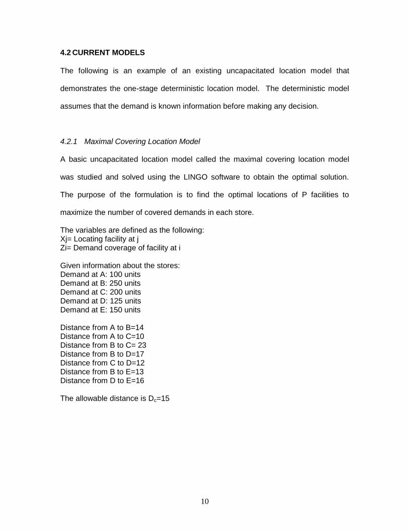
4.2.1 Maximal Covering Location Model
A basic uncapacitated location model called the maximal covering location model
was studied and solved using the LINGO software to obtain the optimal solution.
The purpose of the formulation is to find the optimal locations of P facilities to
maximize the number of covered demands in each store.
The variables are defined as the following: Xj= Locating facility at j Zi= Demand coverage of facility at i Given information about the stores: Demand at A: 100 units Demand at B: 250 units Demand at C: 200 units Demand at D: 125 units Demand at E: 150 units Distance from A to B=14 Distance from A to C=10 Distance from B to C= 23 Distance from B to D=17 Distance from C to D=12 Distance from B to E=13 Distance from D to E=16 The allowable distance is Dc=15

11
The Diagram of the example is illustrated in the following Figure 4.1. Max Covering Diagram
Dc=15
Figure 4.1 - Demand Network for Maximal Covering Location Model The formulation to maximize covering demand is as follows:
Maximize 100ZA+250ZB+200ZC+125ZD+150ZE (1)
Subject to
ZA <=XA+XB+XC (2)
ZB <= XA+XB+ XE (3)
ZC <=XA+ XC+XD (4)
ZD <= XC+XD (5)
ZE <= XB+ XE (6)
XA+XB+XC+XD+XE=P (7)
All variables 0 or 1 (8)
C
A B
D
E
14
10 23
17
13
16 12
150
125 200
100 250

12
Equation (1) indicates that total covered demands of the store at each facility must
be maximized. Equations (2)-(6) illustrate the linkage constraints of the problem.
Equation (2) specifies that demand at A will not be covered unless at least one
facility is located at A, B or C. Similarly in equations (3)-(6), demand of the location
on the left side of the equation will not be covered unless at least one of the facilities
is located at the locations on the right hand side of the constraints. Since the
allowable distance is Dc=15, only the stores with distances of 15 or less from each
other are considered to be covered via the specific site. For example in equation (2),
demand at point A will only be satisfied if the facilities located at either A with
distance of 0<15, B with distance of 14 <15 or C with distance of 10<15.
Equation (7) illustrates the number of facilities to be built denoted by letter P. This
variable can be changed to any integer number to represent the number of sites that
is allowed to be located in the model. Equation (8) shows the integrality of the
variables used in the formulation.
In order to find the maximal covering solution to this problem, the objective function
and the constraints in Figure 4.2 were entered into LINGO software. Note that in this
example, P is equal to 1. The binary integrality is detonated by the syntax @Bin(Xj)
and @Bin(Zi) in the LINGO model.

13
Figure 4.2 - Lingo Model for Maximal Covering Location Model By looking at the results in Figure 4.3, the maximum amount of demand that can be
covered in this model is 550 shown in the objective value. In order to determine
where the site should be located, the value of the Xj must examined. In this
example, XA has the value one which means that the facility must be located at site
A to cover the demands at point A, B and C.

14
Figure 4.3 - Lingo Solution for Maximal Covering Location Model

15
4.2.2 Weaknesses of Current Models
Given a collection of stores/customers, each with uncertain demand, the principle
questions are:
1. How many distribution centres should be located?
2. Where should these distribution centres be located to cover the most
demand?
3. Which stores/customers should be assigned to each distribution centre?
4. What is the optimal distribution strategy of product for each distribution
centre?
The current uncapacitated location model has several weaknesses.
The most significant weakness of this model is that it fails to address
the issue of uncertain demand. In present location models, averages of
demand of previous years are taken and assigned to the stores. This does
not accurately reflect the uncertainty of the demand and must be addressed
in the new model.
Another limitation of the current model is that it is often dealt with in
isolation. It does not take into account the supply chain as an integrated
whole, but instead each individual element by itself. It does not consider how
the decisions made at one distribution centre will affect the overall profit of the
supply chain. Making a decision that will be beneficial to one component
does not necessarily mean that it will be beneficial to the overall supply chain.

16
Another weakness of the current model is the assumption of infinite
supply of inventory in the distribution centres. This means that costs
associated with liabilities due to excess inventory and lost opportunity are
ignored. Therefore, the only cost that is taken into account is the
transportation costs, which is defined as the cost incurred in moving the
goods from the distribution centres to the stores/customers.

17
To demonstrate the concepts of deterministic and stochastic programming models, a
problem called The Farmer’s Problem in [3] is examined.
4.2.3 The Farmer’s Problem
A farmer specializes in raising grain, corn and sugar beets on his 500 acres of land.
During the winter, he wants to decide how much land to devote to each crop. The
farmer knows that at least 200 tons of wheat and 240 tons of corn are needed for
cattle feed. These can be raised on the farm or bought from a wholesaler. Any
production in excess of the feeding requirement would be sold.
Selling prices are $170 per ton for wheat and $150 per ton for corn. Due to the
wholesaler’s margin and transportation costs, the purchase prices are 40% more
than the selling prices. Another crop is Sugar beet, which sells at $36/T but due to
the imposition of the European Commission quota any amount in excess of 6000T is
sold only at $10/T.
4.2.3.1 Deterministic Model for Farmer’s Problem
Based on past experience, the farmer knows that the mean yield on his land is
approximately 2.5T, 3T and 20T per acre for wheat, corn and sugar beets,
respectively.
Table 4.1 summarizes the given data for the Farmer’s Problem.

18
Table 4.1 - Data for Farmer’s Problem The variables are defined as: x1 = acres of land devoted to wheat, x2 = acres of land devoted to corn, x3 = acres of land devoted to sugar beets, w1 = tons of wheat sold, y1 = tons of wheat purchased, w2 = tons of corn sold, y2 = tons of corn purchased, w3 = tons of sugar beets sold at the favorable price, w4 = tons of sugar beets sold at the lower price. The problem reads as follows: Min 150x1 + 230x2 + 260x3 + 238y1 – 170w1 + 210y2 – 150w2 – 36w3 -10w4 Subject to x1 + x2 +x3 <= 500, 2.5x1 +y1 –w1 >= 200, 3x2 +y2 –w2 >= 240, w3 + w4 <= 20x3, w3<= 6000, x1, x2, x3, y1, y2, w1, w2, w3, w4 >=0. (1.1) In order to solve the linear program to help the farmer decide, the model (1.1) was
entered into a solver and the results are presented in Table 4.2.
Wheat Corn Sugar Beets
Yield (T / acre) 2.5 3 20
Planting cost ($ / acre) 150 230 260
Selling price ($ / T) 170 150 36 under 6000 T 10 above 6000 T
Purchase Price ($ / T) 238 210 -
Min requirement (T) 200 240 -
Total available land: 500 acres
19
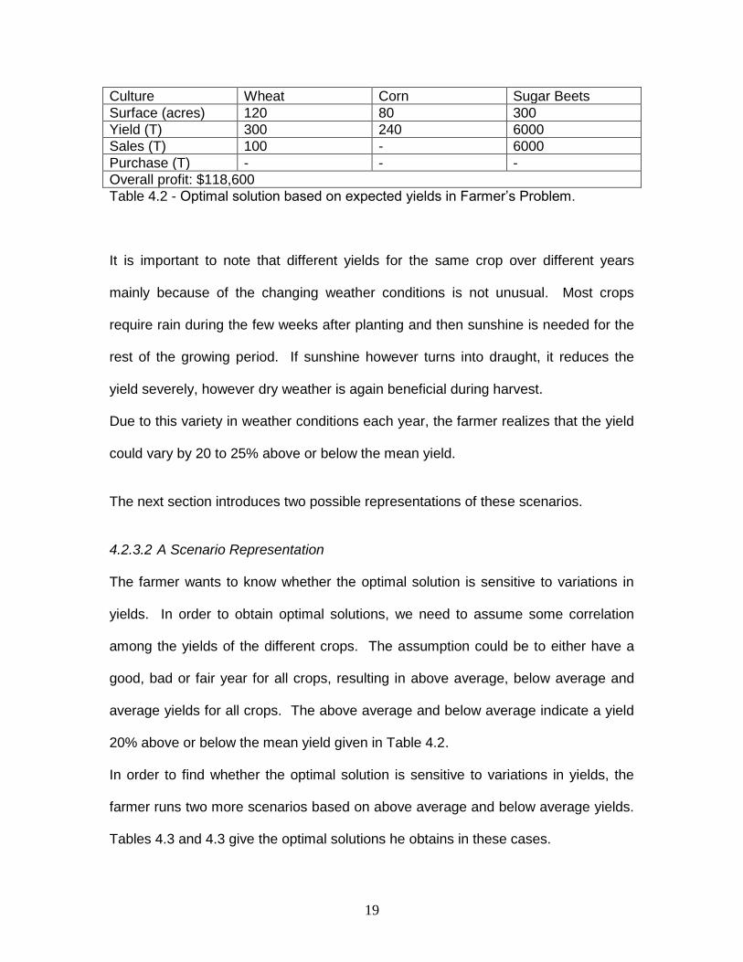
Culture Wheat Corn Sugar Beets
Surface (acres) 120 80 300
Yield (T) 300 240 6000
Sales (T) 100 - 6000
Purchase (T) - - -
Overall profit: $118,600
Table 4.2 - Optimal solution based on expected yields in Farmer’s Problem.
It is important to note that different yields for the same crop over different years
mainly because of the changing weather conditions is not unusual. Most crops
require rain during the few weeks after planting and then sunshine is needed for the
rest of the growing period. If sunshine however turns into draught, it reduces the
yield severely, however dry weather is again beneficial during harvest.
Due to this variety in weather conditions each year, the farmer realizes that the yield
could vary by 20 to 25% above or below the mean yield.
The next section introduces two possible representations of these scenarios. 4.2.3.2 A Scenario Representation The farmer wants to know whether the optimal solution is sensitive to variations in
yields. In order to obtain optimal solutions, we need to assume some correlation
among the yields of the different crops. The assumption could be to either have a
good, bad or fair year for all crops, resulting in above average, below average and
average yields for all crops. The above average and below average indicate a yield
20% above or below the mean yield given in Table 4.2.
In order to find whether the optimal solution is sensitive to variations in yields, the
farmer runs two more scenarios based on above average and below average yields.
Tables 4.3 and 4.3 give the optimal solutions he obtains in these cases.

20
Culture Wheat Corn Sugar Beets
Surface (acres) 183.33 66.67 250
Yield (T) 550 240 6000
Sales (T) 350 - 6000
Purchase (T) - - -
Overall profit: $167,667
Table 4.3 - Optimal solution based on above average yields (+20%) in Farmer’s Problem
Culture Wheat Corn Sugar Beets
Surface (acres) 100 25 375
Yield (T) 200 60 6000
Sales (T) - - -
Purchase (T) - 180 -
Overall profit: $59,950
Table 4.4 - Optimal solution based on below average yields (-20%) in Farmer’s Problem From these tables it can be observed that when the yields are high, smaller surfaces
are needed to raise the minimum requirements in wheat and corn and sugar beet
quota. The remaining land is allocated to wheat and the extra production is sold.
However when the yields are low, larger surfaces are required to raise the minimum
requirements and the sugar beet quota. It is important to note that the corn
requirements are not met and hence some corn must be bought to satisfy the
demand.
4.2.3.3 Stochastic Model for Farmer’s Problem
The farmer realizes that he is unable to make a perfect decision, therefore, he wants
to evaluate the benefits and losses of each decision in each scenario. The scenario
index s= 1,2,3 corresponds to above average, average or below average yields,
respectively. This creates a new set of variables denoted by wis, i=1,2,3,4, s=1,2,3
and yjs, j=1,2, s=1,2,3.

21
If the three scenarios have the same probability, the farmer’s problem can be
formulated as follows:
Min 150x1 + 230x2 + 260x3 –
1/3(170w11 – 238y11 + 150w21- 210y21 + 36w31 +10w41) – 1/3(170w12 – 238y12 + 150w22 – 210y22 + 36w32 +10w42) – 1/3(170w13 – 238y13 + 150w23 -210y23 +36w33 + 10w43)
Subject to x1 + x2 + x3 <=500 3x1 + y11 – w11 >=200 3.6x2 + y21 – w21 >=240 w31 + w41 <=24x3 w31<=6000 2.5x1 + y12 – w12 >=200 3x2 + y22 – w22 >=240 w32 + w42 <=20x3 w32<=6000 2x1 + y13 – w13 >=200 2.4x2 + y23 – w23 >=240 w33 + w43 <=16x3 w33 <=6000 x, y, w >=0 (1.2)
The above formulation is known as the extensive form of stochastic program
because it explicitly describes the second stage decision variables for all scenarios.
The first stage is represented by 150x1 + 230x2 + 260x3 which determines the
amount of land devoted to each crop. It must be decided before realizing the
weather and crop yields. The second stage decisions include the wis and yis
variables which describe the yields, sales and purchases in the three scenarios.
The optimal solution of the above model (1.2) is presented in Table 4.5

22
Wheat Corn Sugar Beets
First Stage Area (acres) 170 80 250
s=1 Above Yield (T) Sales (T) Purchase (T)
510 310
288 48
6000 6000 (fav price)
s=2 Average Yield (T) Sales (T) Purchase (T)
425 225
240 5000 5000 (fav price)
s=3 Below Yield (T) Sales (T) Purchase (T)
340 140
192 48
4000 4000 (fav price)
Overall Profit: $108,390
Table 4.5 - Optimal solution for the stochastic model (1.2) The optimal solution is indicated by avoiding sugar beet sales at the unfavorable
price even if it means that some portion of the quota is unused when yields are
average or below average. However, the corn allocation is such that it should meet
the feeding requirement when yields are average. This means that sales are
possible when yields are above average and purchases are needed when yields are
below average. The rest of the land can be devoted to corn which is large enough to
meet the minimum requirement for cattle feed and sales always occur.
As [5] illustrates in the solution from the stochastic model, under uncertainty, it is
impossible to find an ideal solution under all circumstances. Decisions such as
selling sugar beets at the unfavorable price or having some unused quota never
have to take place if perfect forecast was available. These decisions can be
modeled in the stochastic model because decisions have to be balanced between
different scenarios.
The balancing or hedging effect as it is described by [5] has an important impact on
the expected optimal profit. If the yields vary over years but they are cyclical (a year

23
with above average is always followed by a year with average and then a year with
below average yields), the farmer must take solutions in Table 4.3, Table 4.2 and
Table 4.4, respectively. Following this trend, the farmer will have a profit of
$167,667 the first year, $118,600 the second year, and $59,950 the third year. If the
yields of crops vary randomly, in the long run, if each yield is realized one third of the
years, the farmer will get an expected profit of $115,406 per year. This is the
situation under perfect information. Since the farmer does not get prior information
about the yields of the crops, he needs to take the solution presented in Table 4.5
with a profit of $108,390. The expected value of perfect information (EVPI), which
measures the value of knowing the future with certainty, is equal to the difference of
$155,406 and $108,390 which is equal to $7016.
According to [5], a different approach to making decisions is to assume expected
yields and always to allocate the optimal plating surface according to these yields
which are represented in Table 4.2. This approach results in a long run annual profit
of $107,240 [5]. The value $1150 represents the value of the stochastic solution
(VSS) which is equal to the difference of the expected yield profit and the stochastic
model profit ($108,390-107,240=$1150).
These two quantities, EVPI and VSS create the motivation behind stochastic
programming in general.
4.2.3.4 General model formulation In this section, a general formulation of the stochastic problem is illustrated.
The first stage decisions are the decisions to be taken without full information on
some random events and they are represented by a vector x. For example, in the

24
farming example, the decision is to how to allocate the acres of land to each crop.
Later, when all the information is realized by some random vector ξ, the corrective
actions y or second-stage decisions are taken.
In the farming example, the random vector represents the set of yields and the
second stage corrective actions are purchases and sales of crops. According to [5],
the two-stage stochastic program with recourse form can be written as:
min cTx + EξQ(x, ξ)
Subject to Ax = b, x>=0,
where Q(x, ξ) = min {qTy | Wy = h - Tx, y>=0}.
A second-stage problem for one particular scenario s can be written as Q(x, s) = min {238y1 -170w1 + 210y2 – 150w2 -36w3 – 10w4} Subject to t1(s)x1 + y1 – w1 >= 200, t2(s)x2 + y2 – w2 >= 240, w3 + w4 <= t3(s) x3, w3 <= 6000, y1, w1 <=0,
where ti(s) represents the yield of crop i under scenario s. The random vector ξ = (t1, t2,
t3) is generated by the three yields and ξ can take on three different values, say ξ1, ξ2, ξ3
which represent (t1(1), t2(1), t3(1)), (t1(2), t2(2), t3(2)) and (t1(3), t2(3), t3(3)).

25
5. SUPPLY CHAIN DESIGN FOR DISTRIBUTION CENTRES
General Assumptions:
Costs associated with the model are locating costs and transportation costs
Overall capacity of all the distribution centres are more than the expected
demand
It is feasible to deliver from a distribution centre to any demand point
5.1 DETERMINISTIC MODEL FORMULATION (MODEL 1)
The objective of this model is to reformulate the set covering location model to have
an asset reliability structure and also to provide a foundation for the comparison of
the deterministic model with stochastic structure (MODEL 2) vs. the stochastic model
(MODEL 3) solved independently. The main weakness of this model is that it does
not take into account the uncertainty of demand. It takes the average over all
different scenarios and it assumes that it is the expected demand at point i.
The variables used in the model are defined as follows: Di= Average demand at point i P = # of distribution centres allowable Ci=Cost of locating distribution centre i h=Unit price of product Tij= Cost of transporting one unit of product from distribution centre i to demand point j Xi = Location decision for distribution centre i Yij= Amount of demand satisfied at demand point j by distribution centre i n= number of demand points Lj= Capacity available at location j

26
OBJECTIVE FUNCTION:
MIN n
i
n
i
n
j
YijTijhXiCi1 1 1
*)(* (1)
CONSTRAINTS SUBJECT TO:
n
i
PXi1
(1)
n
i
n
j
DiYij1 1
i= 1,2,…n (2)
XiLjYij * i= 1, 2,…n (3)
j= 1, 2,…n Xi = {0,1} (4)
Objective Function:
Looking at the model presented above, the location decision variables are denoted
by Xi and are multiplied by the locating costs (Ci). The location variables indicate
whether to locate the distribution centres at Xi. Since the variables are binary, if a
distribution centre is located at Xi then the variable Xi will be equal to 1. Similarly, if
a distribution centre is not located at Xi, then Xi will be equal to 0.
Another variable included in the objective function is the number of units allocated
from distribution centres to the demand points, which is denoted by Yij. This variable
is multiplied by the unit price of the product (h) minus the transportation cost (Tij) for
moving one unit of product from distribution centre i to demand point j.
Constraints:
Constraint (1): This constraint indicates that the total number of all the distribution
centres located in the network of demand is equal to a predetermined number. The

27
factors that could govern this number are budget constraints, feasibility issues and
land availability.
Constraint (2): This constraint specifies that the average demand at each demand
point has to be satisfied.
Constraint (3): This constraint ensures that the capacity constraints at distribution
centres are not exceeded by the distribution of products.
Constraint (4): This constraint defines the variables Xi as binary meaning they can
only be 1 or 0.
5.2 STOCHASTIC MODEL FORMULATION (MODEL 3) In order to capture the uncertainty of the demand points within the model, the
following two-stage stochastic model is developed with a probability framework and
an asset reliability structure.
The variables used in the model are defined as follows: Djs= Amount of demand at point j under scenario s P = # of distribution centres allowable Ci=Cost of locating distribution centre i h=Unit price of product Tij= Cost of transporting one unit of product from distribution centre i to demand point j Xi = Location decision for distribution centre i Yijs= Amount of demand satisfied at demand point j by distribution centre i under scenario s Ps= Probability of scenario s occurring n= number of demand points m= number of scenarios Lj= Capacity available at location j

28
OBJECTIVE FUNCTION:
MIN n
i
m
s
n
i
n
j
YijsTijhPsXiCi1 1 1 1
*)(** (1)
CONSTRAINTS SUBJECT TO:
n
i
PXi1
(2)
m
s
n
i
n
j
DjsYijs1 1 1
(3)
XiLjYijs * i= 1, 2,…n (4)
j= 1, 2,…n s= 1, 2,…m Xi = {0,1} (5) The main difference between the stochastic model and the deterministic model is
that it considers risks associated with the uncertainty of expected demand. In order
to accomplish this, multiple scenarios of demand are considered in this model.
There is a probability assigned to each scenario which indicates the likelihood of
each demand level occurring.

29
6. APPLICATION OF MODEL
To apply these models in a practical situation, a case representing a hypothetical
company with all the necessary information is developed and used in the
deterministic and stochastic models.
6.1 DATA In Table 6.1, the demand values for each demand point for each scenario are
presented. In this particular case, there are a total of three scenarios (S1, S2, S3)
and four demand points (A, B, C, D). The unit price of the product is $10.
Scenario one (S1) represents the low demand, scenarios two (S2) represents the
medium demand and the last scenario (S3) represents the high demand. There is a
probability of one third assigned to the occurrence of each scenario.
DEMAND POINTS
A B C D
S1 50 100 65 70
S2 125 300 250 175
S3 800 750 255 810
Table 6.1 – Amount of demand at each point for each scenario for case Table 6.2 shows the transportation costs to move one unit of product between a
distribution centre to a certain demand point.
DEMAND POINTS
A B C D
A 0 14 10 0
B 14 0 23 17
C 10 23 0 12
D 0 17 12 0
Table 6.2 – Transportation costs to move one unit of product between points for case

30
Table 6.3 specifies the costs of location distribution centre.
DEMAND POINTS
A B C D
1000 1500 1200 1100
Table 6.3 – Cost of locating a distribution centre for case
6.2 DETERMINISTIC AND STOCHASTIC MODELS INCLUDING THE CASE In this section, the extensive form of all the models are shown using the information
developed in the case.
6.2.1 MODEL 1
Deterministic Model in LINGO:
MIN=1000*X1 + 1500*X2 + 1200*X3 + 1100*X4 -(10*y111 + 10*y121 + 10*y131 + 10*y141+ 10*y211 + 10*y221 + 10*y231 + 10*y241 + 10*y311 + 10*y321 + 10*y331 + 10*y341 + 10*y411 + 10*y421 + 10*y431 + 10*y441 - (0*y111+ 14*y121 + 10*y131)- (14*y211+ 0*y221 + 23*y231 + 17*y241)- (10*y311+ 23*y321+ 0*y331 + 12*y341)- (17*y421+ 12*y431+ 0*y441) ) ; X1+X2+X3+X4=2; 325=y111+y211+y311+y411; 383=y121+y221+y321+y421; 190=y131+y231+y331+y431; 352=y141+y241+y341+y441; y111<=450*X1; y121<=450*X1; y131<=450*X1; y141<=450*X1; y211<=150*X2; y221<=150*X2;

31
y231<=150*X2; y241<=150*X2; y311<=450*X3; y321<=450*X3; y331<=450*X3; y341<=450*X3; y411<=750*X4; y421<=750*X4; y431<=750*X4; y441<=750*X4; @BIN (X1); @BIN (X2); @BIN (X3); @BIN (X4); By using LINGO software, this model was solved with the final objective function
cost of -$4938. The resulting first-stage location decisions: X1=1, X2=0, X3=1,
X4=0.
The second-stage decisions were: Y111=325, Y121=383, Y141=352, and Y331=190
with the rest equal to 0. A more detailed solution can be found in Appendix A.
6.2.2 MODEL 2
Deterministic Model with Stochastic Structure in LINGO:
The first stage decisions (X variables) from the deterministic model are used (X1=1,
X2=0, X3=1, X4=0) to solve the deterministic model with stochastic structure for the
corrective actions (Y variables).

32
MIN=1000*1 + 1500*0 + 1200*1 + 1100*0 -1/3*(10*y111 + 10*y121 + 10*y131 + 10*y141+ 10*y211 + 10*y221 + 10*y231 + 10*y241 + 10*y311 + 10*y321 + 10*y331 + 10*y341 + 10*y411 + 10*y421 + 10*y431 + 10*y441 - (0*y111+ 14*y121 + 10*y131)- (14*y211+ 0*y221 + 23*y231 + 17*y241)- (10*y311+ 23*y321+ 0*y331 + 12*y341)- (17*y421+ 12*y431+ 0*y441) ) -1/3*(10*y112 + 10*y122 + 10*y132 + 10*y142+ 10*y212 + 10*y222 + 10*y232 + 10*y242+ 10*y312 + 10*y322 + 10*y332 + 10*y342+ 10*y412 + 10*y422 + 10*y432 + 10*y442- (0*y112+ 14*y122 + 10*y132)- (14*y212+ 0*y222 + 23*y232 + 17*y242)- (10*y312+ 23*y322+ 0*y332 + 12*y342)- (17*y422+ 12*y432+ 0*y442) ) -1/3*(10*y113 + 10*y123 + 10*y133 + 10*y143 + 10*y213 + 10*y223 + 10*y233 + 10*y243 + 10*y313 + 10*y323 + 10*y333 + 10*y343 + 10*y413 + 10*y423 + 10*y433 + 10*y443 - (0*y113+ 14*y123 + 10*y133)- (14*y213+ 0*y223 + 23*y233 + 17*y243)- (10*y313+ 23*y323+ 0*y333 + 12*y343)- (17*y423+ 12*y433+ 0*y443) ); 50=y111+y211+y311+y411; 125=y112+y212+y312+y412; 800=y113+y213+y313+y413; 100=y121+y221+y321+y421; 300=y122+y222+y322+y422; 750=y123+y223+y323+y423; 65=y131+y231+y331+y431; 250=y132+y232+y332+y432; 255=y133+y233+y333+y433; 70=y141+y241+y341+y441; 175=y142+y242+y342+y442; 810=y143+y243+y343+y443; y111<=450*1; y121<=450*1; y131<=450*1; y141<=450*1;

33
y112<=450*1; y122<=450*1; y132<=450*1; y142<=450*1; y113<=450*1; y123<=450*1; y133<=450*1; y143<=450*1; y211<=150*0; y221<=150*0; y231<=150*0; y241<=150*0; y212<=150*0; y222<=150*0; y232<=150*0; y242<=150*0; y213<=150*0; y223<=150*0; y233<=150*0; y243<=150*0; y311<=450*1; y321<=450*1; y331<=450*1; y341<=450*1; y312<=450*1; y322<=450*1; y332<=450*1; y342<=450*1; y313<=450*1; y323<=450*1; y333<=450*1; y343<=450*1; y411<=750*0; y421<=750*0; y431<=750*0; y441<=750*0; y412<=750*0; y422<=750*0; y432<=750*0; y442<=750*0;

34
y413<=750*0; y423<=750*0; y433<=750*0; y443<=750*0;
By using LINGO software, this model was solved with the final objective function
cost of -$1427. The detailed solution can be found in Appendix B.
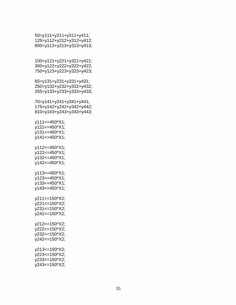
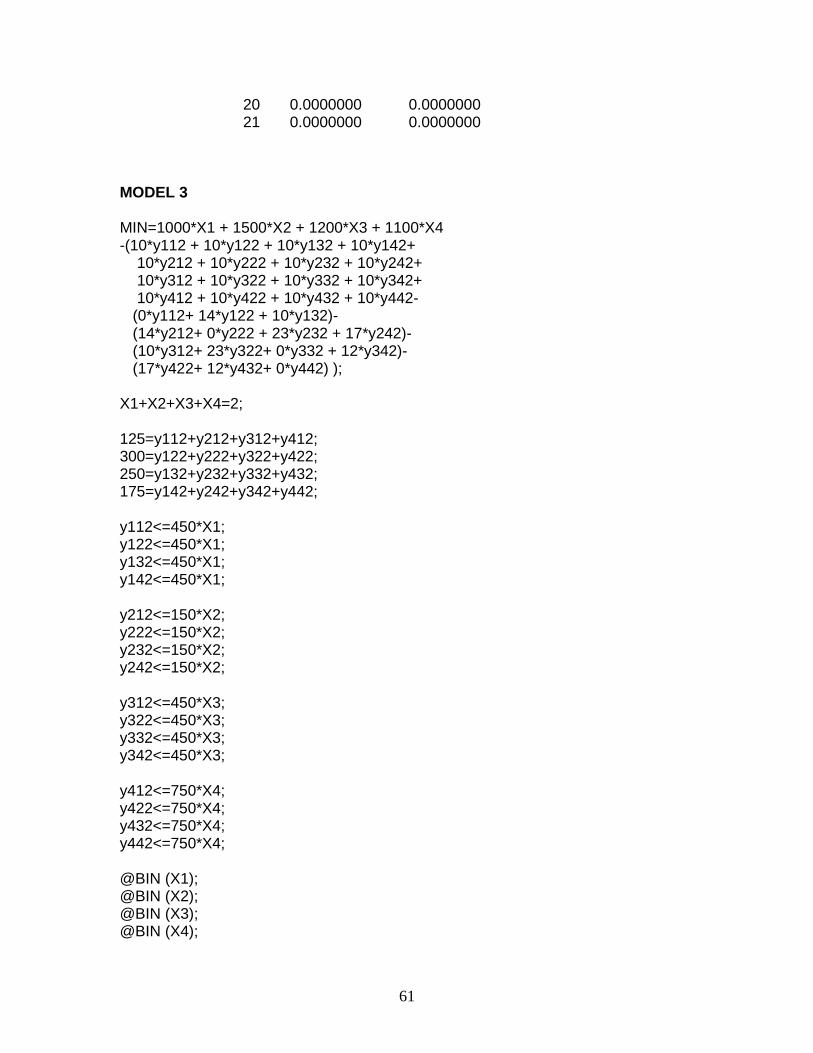
6.2.3 MODEL 3
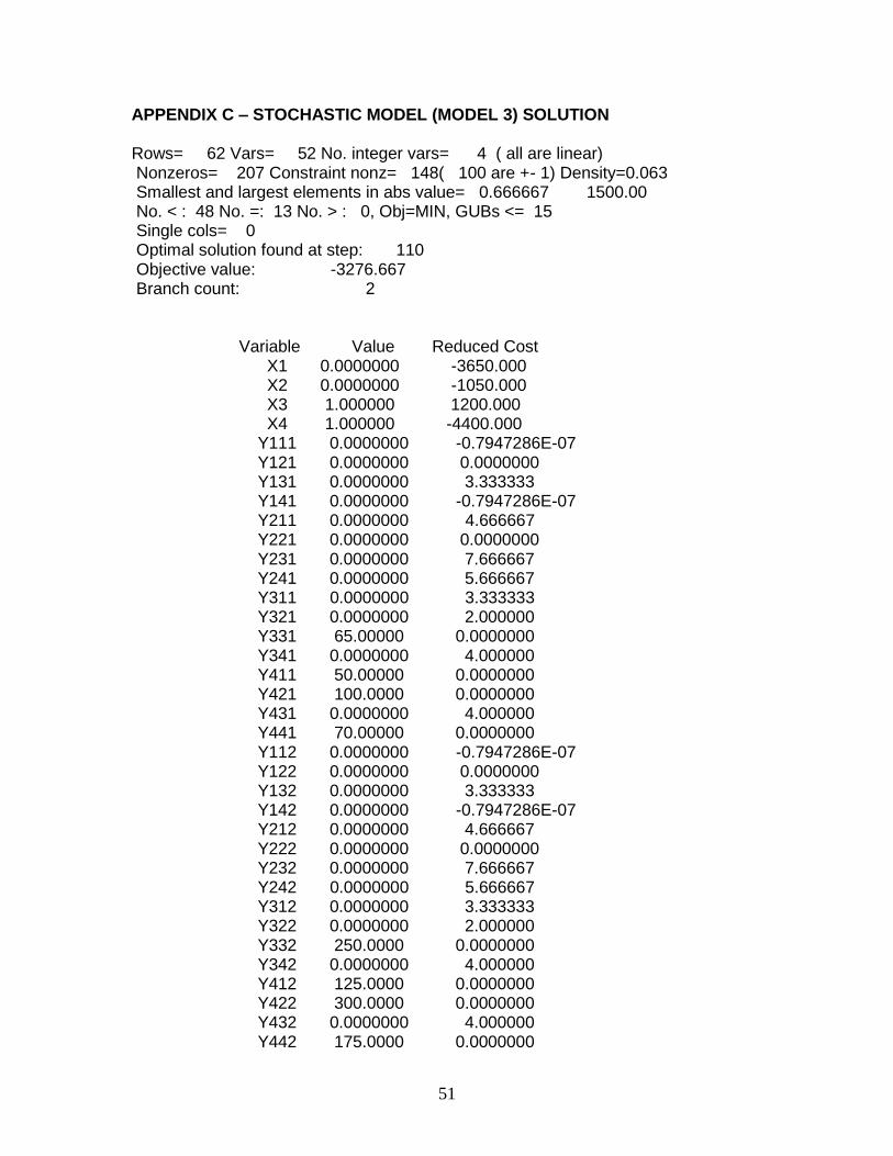
Stochastic Model in LINGO:
This stochastic model is solved independently of the deterministic model for both the
first-stage and second-stage variables.
MIN=1000*X1 + 1500*X2 + 1200*X3 + 1100*X4 -1/3*(10*y111 + 10*y121 + 10*y131 + 10*y141+ 10*y211 + 10*y221 + 10*y231 + 10*y241 + 10*y311 + 10*y321 + 10*y331 + 10*y341 + 10*y411 + 10*y421 + 10*y431 + 10*y441 - (0*y111+ 14*y121 + 10*y131)- (14*y211+ 0*y221 + 23*y231 + 17*y241)- (10*y311+ 23*y321+ 0*y331 + 12*y341)- (17*y421+ 12*y431+ 0*y441) ) -1/3*(10*y112 + 10*y122 + 10*y132 + 10*y142+ 10*y212 + 10*y222 + 10*y232 + 10*y242+ 10*y312 + 10*y322 + 10*y332 + 10*y342+ 10*y412 + 10*y422 + 10*y432 + 10*y442- (0*y112+ 14*y122 + 10*y132)- (14*y212+ 0*y222 + 23*y232 + 17*y242)- (10*y312+ 23*y322+ 0*y332 + 12*y342)- (17*y422+ 12*y432+ 0*y442) ) -1/3*(10*y113 + 10*y123 + 10*y133 + 10*y143 + 10*y213 + 10*y223 + 10*y233 + 10*y243 + 10*y313 + 10*y323 + 10*y333 + 10*y343 + 10*y413 + 10*y423 + 10*y433 + 10*y443 - (0*y113+ 14*y123 + 10*y133)- (14*y213+ 0*y223 + 23*y233 + 17*y243)- (10*y313+ 23*y323+ 0*y333 + 12*y343)- (17*y423+ 12*y433+ 0*y443) ); X1+X2+X3+X4=2;
35
50=y111+y211+y311+y411; 125=y112+y212+y312+y412; 800=y113+y213+y313+y413; 100=y121+y221+y321+y421; 300=y122+y222+y322+y422; 750=y123+y223+y323+y423; 65=y131+y231+y331+y431; 250=y132+y232+y332+y432; 255=y133+y233+y333+y433; 70=y141+y241+y341+y441; 175=y142+y242+y342+y442; 810=y143+y243+y343+y443; y111<=450*X1; y121<=450*X1; y131<=450*X1; y141<=450*X1; y112<=450*X1; y122<=450*X1; y132<=450*X1; y142<=450*X1; y113<=450*X1; y123<=450*X1; y133<=450*X1; y143<=450*X1; y211<=150*X2; y221<=150*X2; y231<=150*X2; y241<=150*X2; y212<=150*X2; y222<=150*X2; y232<=150*X2; y242<=150*X2; y213<=150*X2; y223<=150*X2; y233<=150*X2; y243<=150*X2;

36
y311<=450*X3; y321<=450*X3; y331<=450*X3; y341<=450*X3; y312<=450*X3; y322<=450*X3; y332<=450*X3; y342<=450*X3; y313<=450*X3; y323<=450*X3; y333<=450*X3; y343<=450*X3; y411<=750*X4; y421<=750*X4; y431<=750*X4; y441<=750*X4; y412<=750*X4; y422<=750*X4; y432<=750*X4; y442<=750*X4; y413<=750*X4; y423<=750*X4; y433<=750*X4; y443<=750*X4; @BIN (X1); @BIN (X2); @BIN (X3); @BIN (X4); By using LINGO software, this model was solved with the final objective function
cost of - $3276. The resulting first-stage location decisions: X1=0, X2=0, X3=3,
X4=4. A more detailed solution can be found in Appendix C.
Demand Points
Scenario
Deterministic Model Cost MODEL 1
Deterministic Model with Stochastic Structure Cost MODEL 2
Stochastic Model Cost MODEL 3
Benefit of Stochastic Model
Original -4938 -1426 -3276 -1850
Table 6.4 - Costs for each model in case

37
Looking at Table 6.4, it becomes apparent that there is a reduction in cost in the
stochastic model when compared to Model 2, which is evidence that there are
benefits when uncertainty of demands is taken into account.
These benefits are discussed in further detail in the next section.

38
7. RESULTS
In this section the models are evaluated in order to determine the value of the
stochastic model developed in this thesis. There will be two main areas of focus:
1. Scenario Comparisons between Model 2 and Model 3
2. Effect of Demand Variability on Model Results
7.1 SCENARIO COMPARISON OF MODEL 2 AND MODEL 3
In this section, each scenario (S1, S2 and S3) in model 3 is compared to model 2 to
determine whether each scenario in the stochastic model will give better results in
terms of minimization of costs. In order to determine the benefits of the Stochastic
Model (Model 3) for each particular scenario, the following procedure is taken:
1. The deterministic model (Model 1) is solved using the Lingo software
2. The location decisions (Xi’s) found in Step 1 are plugged into the
deterministic model with stochastic structure (Model 2) and solved
3. The stochastic model (Model 3) is solved by isolating the appropriate
scenario (the constraints related to other scenarios are removed)
4. The resulting costs for Models 2 and 3 are compared

39
First Scenario (Low Demand):
After solving Model 1, the cost is -$4938 and is presented in Table 7.1. The location
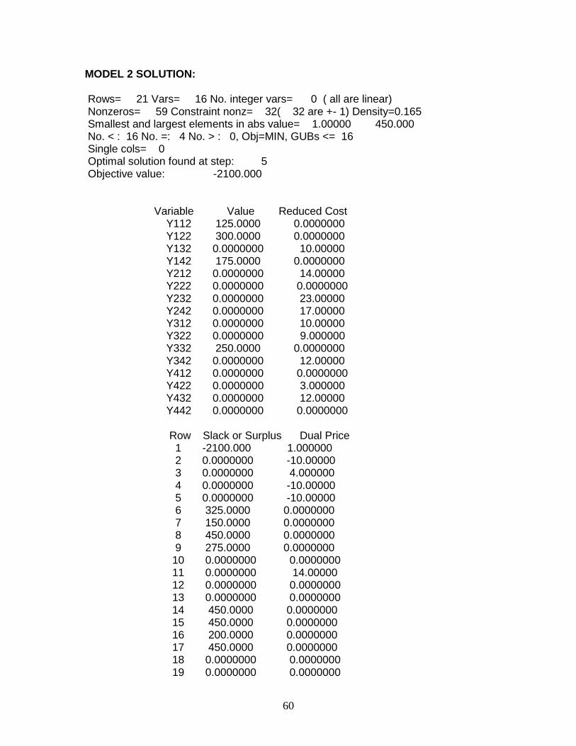
decisions are to locate at X1 and X3. The cost for Model 2 is $750. Solving Model 3
results in a cost of $300, however it is important to note that the location decisions
are changed to X1 and X2. By comparing the costs from Model 2 and 3 models, it
can be established that the stochastic model for the first scenario does better in
minimizing the cost since $300 is less than $750. The cost comparisons are
represented in Table 7.1. The detailed models and solutions can be seen in
Appendix D.
Second Scenario (Medium Demand):
Same technique of comparison is repeated for the second scenario, S2. As
illustrated in Table 7.1, again it is evident that the cost of stochastic model for
scenario 2 is the same value as the deterministic model with stochastic structure.
The cost of stochastic model (-$2100) is the same value as the deterministic model
with stochastic structure. The location decisions, locating at X1 and X3 also stay the
same as the deterministic model. The detailed models and solutions can be seen in
Appendix E.
Third Scenario (High Demand):
The comparison is done for the third scenario, s3. Looking at the results in Table
7.1, it can be concluded that the cost of stochastic model of -$10100 is smaller than
the cost of model with deterministic solutions (-$2930). The location decisions are
changed from locating at X1 and X3 to locating at X1 and X4 in the stochastic model.
However the cost does not fall within the original deterministic model (Model 1) and

40
the deterministic with stochastic structure model (Model 2). This might be due to the
fact that demand for scenario 3 is considerably higher comparing to the other
scenarios. The capacity at X1 and X3 are not enough to satisfy the demand at each
point, and therefore the location decision is changed to X1 and X4.
The detailed models and solutions can be seen in Appendix F.
Demand Points
Scenarios
Deterministic Model Cost (MODEL 1)
Deterministic Model with Stochastic Structure Cost (MODEL 2)
Stochastic Model Cost (MODEL 3)
Benefits of Model 3
S1 -4938 750 300 -450 S2 -4938 -2100 -2100 0 S3 -4938 -2930 -10100 -7170
Table 7.1 – Cost comparison of scenarios in case
Looking at the results in Table 7.1, it is evident that in all three scenarios, Model 3
had lower costs than that of Model 2. This means that no matter what scenario
occurs in the real world (low, medium, high) demand, in general, the results for
Model 3 will be better than that of Model 2.

41
7.2 COMPARISON OF DIFFERENT DEGREES OF VARIANCE IN DEMAND
In order to determine the benefits of the new model, it is crucial to evaluate the
effects of demand variability on all models. Variability does not play a role in the
deterministic model, because the model assumes that demand is known information
and is calculated by taking the average of all of the demand values for all scenarios.
In contrast to the deterministic model, the stochastic model developed in this thesis
project takes into account the possibility of different customer demand values and
assigns them to a particular scenario. In this thesis, there are three possible
scenarios of demand: Low (S1), Medium (S2), and High (S3).
The original case is developed and the following demand points in Table 7.2 are
assigned to each scenario.
Demand Points
Scenarios 1 2 3 4 Average of
Demand Standard Deviation
Original S1 50 100 65 70 71.25 20.97
Original S2 125 300 250 175 212.5 77.73
Original S3 800 750 255 810 653.75 267.13
Table 7.2 – Demand values of 3 scenarios in case
With these values, the following costs are determined with LINGO software for the
different models. This is a clear indication that once demand uncertainty is
considered, the overall benefits are significant. In this particular example, the final
objective value for cost is - $1426.00 when just taking averages of demand, while
the cost for the stochastic model is - $3276.00. This means that there is an
additional profit of $1850 for the stochastic model.

42
To conduct a more in depth analysis of the effect of variability on the results of the
models, 3 more scenarios of demand are created (A, B, C). Within these three
scenarios, the average of the demand remains the same as the original case, but the
standard deviation (and therefore variance of demand) is reduced (with C having the
lowest standard deviation). The new demand values in scenarios A, B, and C can be
seen in Table 7.3.
The different models and solutions for each scenario of demand variance A, B, and
C can be found in Appendices G, H, and I respectively.
Demand Points
Scenarios 1 2 3 4 Average of Demand
Standard Deviation
Original S1 50 100 65 70
71.25
20.97 A 60 80 70 75 8.54 B 63 74 71 77 6.02 C 69 69 71 76 3.30
Original S2 125 300 250 175
212.5
77.73 A 175 235 224 216 26.19 B 191 224 219 216 14.71 C 206 216 213 215 4.51
Original S3 800 750 255 810
653.75
267.13 A 701 645 559 710 69.40 B 675 650 625 665 21.75
C 645 672 649 649 12.31
Originalavg 325.00 383.33 190.00 351.67 Aavg 312.00 320.00 284.33 333.67 Bavg 309.67 316.00 305.00 319.33 Cavg 306.67 319.00 311.00 313.33
Table 7.3 – Demand values of scenarios of difference variance in case
Demand Points
Scenarios
Deterministic Model Cost (MODEL 1)
Deterministic Model with Stochastic Structure Cost (MODEL 2)
Stochastic Model Cost (MODEL 3)
Benefit of Stochastic
Model
Original -4938 -1426 -3276 -1850 A -5820 -2995 -4324 -1329 B -5876 -3082 -4128 -1046 C -5834 -3058 -3981 -923
Table 7.4 - Costs for variance scenarios A, B, and C for models in case
Decreasing Variability

43
Looking at the results in Table 7.4, it is clear that variability plays a significant role in
the resulting costs for each model. As variability of the demand in the model
increases, so do the benefits of the stochastic model. However, it should be noted
that even when the variability is very low, as in the case of scenario C, the benefits
of the stochastic model (reduction of $923 of cost) is still a considerable amount.

44
8. CONCLUSION
It can be concluded that, in comparing each scenario from Model 3 with Model 2, all
of the scenarios in Model 3 perform equally well or better than Model 2 in terms of
cost. This is due to the fact that stochastic model takes into account the location
decisions at the same time as the uncertainty of each scenario happening. It is
because of this flexibility that the objective function is able to provide a lower cost
than in Model 2.
It is also clear that variability plays a significant role in the resulting costs for each
model. The outcomes suggest that variability has a direct relationship to the
objective function. In this particular case, as variability of the demand in the model
increases, so do the benefits of the stochastic model. This is further evidence that a
stochastic model would be greatly beneficial in a real-world situation where any type
of uncertainty is involved.
Decisions have to be balanced or hedged against the various scenarios and hence it
impacts the expected optimal profit. In a real world problem where perfect
information is not available and decisions must be made beforehand, the stochastic
model provides a tool to the decision maker to better optimize the objective function
of the problem. In the stochastic model (MODEL 3), the location decisions (which
are the first-stage decisions) are unknown and the second-stage takes corrective
action to optimize the objective function as it solves the two stages simultaneously
resulting in a lower cost than the Model 2.

45
9. REFERENCES
[1] M. Attaran, (2003), “Information Technology and Business Process Redesign”, Business Process Management Journal, Vol.9, No. 4, pp.440-458
[2] “Supply Chain Management”, [Online Document], 2007 March 10, [cited 2007
March 12], Available HTTP: http://en.wikipedia.org/wiki/Supply_chain_management
[3] Mulvey JM, Vladimirou H. Stochastic Network Programming for Financial
Planning Problems [4] Mulvey JM, Shetty B. Financial Planning Via Multi-Stage Stochastic
Optimization. Computers and operations Research 31 (2004) 1-20. [5] J.R. Birge, F. Louveaux, Introduction to Stochastic Programming, New York:
Springer-Verlag, 1997

46
10. APPENDICES
APPENDIX A – DETERMINISTIC MODEL (MODEL 1) SOLUTION Rows= 22 Vars= 20 No. integer vars= 4 ( all are linear) Nonzeros= 75 Constraint nonz= 52( 36 are +- 1) Density=0.162 Smallest and largest elements in abs value= 1.00000 1500.00 No. < : 16 No. =: 5 No. > : 0, Obj=MIN, GUBs <= 7 Single cols= 0 Optimal solution found at step: 31 Objective value: -4938.000 Branch count: 1 Variable Value Reduced Cost X1 1.000000 1000.000 X2 0.0000000 -600.0000 X3 1.000000 1200.000 X4 0.0000000 1100.000 Y111 325.0000 0.0000000 Y121 383.0000 0.0000000 Y131 0.0000000 10.00000 Y141 352.0000 0.0000000 Y211 0.0000000 14.00000 Y221 0.0000000 0.0000000 Y231 0.0000000 23.00000 Y241 0.0000000 17.00000 Y311 0.0000000 10.00000 Y321 0.0000000 9.000000 Y331 190.0000 0.0000000 Y341 0.0000000 12.00000 Y411 0.0000000 0.0000000 Y421 0.0000000 3.000000 Y431 0.0000000 12.00000 Y441 0.0000000 0.0000000 Row Slack or Surplus Dual Price 1 -4938.000 1.000000 2 0.0000000 0.0000000 3 0.0000000 -10.00000 4 0.0000000 4.000000 5 0.0000000 -10.00000 6 0.0000000 -10.00000 7 125.0000 0.0000000 8 67.00000 0.0000000 9 450.0000 0.0000000 10 98.00000 0.0000000 11 0.0000000 0.0000000

47
12 0.0000000 14.00000 13 0.0000000 0.0000000 14 0.0000000 0.0000000 15 450.0000 0.0000000 16 450.0000 0.0000000 17 260.0000 0.0000000 18 450.0000 0.0000000 19 0.0000000 0.0000000 20 0.0000000 0.0000000 21 0.0000000 0.0000000 22 0.0000000 0.0000000

48
APPENDIX B – DETERMINISTIC MODEL WITH STOCHASTIC STRUCTURE (MODEL 2) SOLUTION Rows= 61 Vars= 48 No. integer vars= 0 ( all are linear) Nonzeros= 175 Constraint nonz= 96( 96 are +- 1) Density=0.059 Smallest and largest elements in abs value= 0.666667 810.000 No. < : 48 No. =: 12 No. > : 0, Obj=MIN, GUBs <= 48 Single cols= 0 Optimal solution found at step: 15 Objective value: -1426.667 Variable Value Reduced Cost Y111 50.00000 0.0000000 Y121 100.0000 0.0000000 Y131 0.0000000 3.333333 Y141 70.00000 0.0000000 Y211 0.0000000 4.666667 Y221 0.0000000 0.0000000 Y231 0.0000000 7.666667 Y241 0.0000000 5.666667 Y311 0.0000000 3.333333 Y321 0.0000000 3.000000 Y331 65.00000 0.0000000 Y341 0.0000000 4.000000 Y411 0.0000000 -0.7947286E-07 Y421 0.0000000 1.000000 Y431 0.0000000 4.000000 Y441 0.0000000 -0.7947286E-07 Y112 125.0000 0.0000000 Y122 300.0000 0.0000000 Y132 0.0000000 3.333333 Y142 175.0000 0.0000000 Y212 0.0000000 4.666667 Y222 0.0000000 0.0000000 Y232 0.0000000 7.666667 Y242 0.0000000 5.666667 Y312 0.0000000 3.333333 Y322 0.0000000 3.000000 Y332 250.0000 0.0000000 Y342 0.0000000 4.000000 Y412 0.0000000 -0.7947286E-07 Y422 0.0000000 1.000000 Y432 0.0000000 4.000000 Y442 0.0000000 -0.7947286E-07 Y113 450.0000 0.0000000 Y123 450.0000 0.0000000 Y133 0.0000000 3.333333 Y143 450.0000 0.0000000

49
Y213 0.0000000 1.333333 Y223 0.0000000 0.0000000 Y233 0.0000000 7.666667 Y243 0.0000000 1.666667 Y313 350.0000 0.0000000 Y323 300.0000 0.0000000 Y333 255.0000 0.0000000 Y343 360.0000 0.0000000 Y413 0.0000000 0.0000000 Y423 0.0000000 0.0000000 Y433 0.0000000 4.000000 Y443 0.0000000 0.0000000 Row Slack or Surplus Dual Price 1 -1426.667 1.000000 2 0.0000000 -3.333333 3 0.0000000 -3.333333 4 0.0000000 0.0000000 5 0.0000000 1.333333 6 0.0000000 1.333333 7 0.0000000 4.333333 8 0.0000000 -3.333333 9 0.0000000 -3.333333 10 0.0000000 -3.333333 11 0.0000000 -3.333333 12 0.0000000 -3.333333 13 0.0000000 0.6666667 14 400.0000 0.0000000 15 350.0000 0.0000000 16 450.0000 0.0000000 17 380.0000 0.0000000 18 325.0000 0.0000000 19 150.0000 0.0000000 20 450.0000 0.0000000 21 275.0000 0.0000000 22 0.0000000 3.333333 23 0.0000000 3.000000 24 450.0000 0.0000000 25 0.0000000 4.000000 26 0.0000000 0.0000000 27 0.0000000 4.666667 28 0.0000000 0.0000000 29 0.0000000 0.0000000 30 0.0000000 0.0000000 31 0.0000000 4.666667 32 0.0000000 0.0000000 33 0.0000000 0.0000000 34 0.0000000 0.0000000 35 0.0000000 7.666667

50
36 0.0000000 0.0000000 37 0.0000000 0.0000000 38 450.0000 0.0000000 39 450.0000 0.0000000 40 385.0000 0.0000000 41 450.0000 0.0000000 42 450.0000 0.0000000 43 450.0000 0.0000000 44 200.0000 0.0000000 45 450.0000 0.0000000 46 100.0000 0.0000000 47 150.0000 0.0000000 48 195.0000 0.0000000 49 90.00000 0.0000000 50 0.0000000 0.0000000 51 0.0000000 0.0000000 52 0.0000000 0.0000000 53 0.0000000 0.0000000 54 0.0000000 0.0000000 55 0.0000000 0.0000000 56 0.0000000 0.0000000 57 0.0000000 0.0000000 58 0.0000000 3.333333 59 0.0000000 2.000000 60 0.0000000 0.0000000 61 0.0000000 4.000000
51
APPENDIX C – STOCHASTIC MODEL (MODEL 3) SOLUTION Rows= 62 Vars= 52 No. integer vars= 4 ( all are linear) Nonzeros= 207 Constraint nonz= 148( 100 are +- 1) Density=0.063 Smallest and largest elements in abs value= 0.666667 1500.00 No. < : 48 No. =: 13 No. > : 0, Obj=MIN, GUBs <= 15 Single cols= 0 Optimal solution found at step: 110 Objective value: -3276.667 Branch count: 2 Variable Value Reduced Cost X1 0.0000000 -3650.000 X2 0.0000000 -1050.000 X3 1.000000 1200.000 X4 1.000000 -4400.000 Y111 0.0000000 -0.7947286E-07 Y121 0.0000000 0.0000000 Y131 0.0000000 3.333333 Y141 0.0000000 -0.7947286E-07 Y211 0.0000000 4.666667 Y221 0.0000000 0.0000000 Y231 0.0000000 7.666667 Y241 0.0000000 5.666667 Y311 0.0000000 3.333333 Y321 0.0000000 2.000000 Y331 65.00000 0.0000000 Y341 0.0000000 4.000000 Y411 50.00000 0.0000000 Y421 100.0000 0.0000000 Y431 0.0000000 4.000000 Y441 70.00000 0.0000000 Y112 0.0000000 -0.7947286E-07 Y122 0.0000000 0.0000000 Y132 0.0000000 3.333333 Y142 0.0000000 -0.7947286E-07 Y212 0.0000000 4.666667 Y222 0.0000000 0.0000000 Y232 0.0000000 7.666667 Y242 0.0000000 5.666667 Y312 0.0000000 3.333333 Y322 0.0000000 2.000000 Y332 250.0000 0.0000000 Y342 0.0000000 4.000000 Y412 125.0000 0.0000000 Y422 300.0000 0.0000000 Y432 0.0000000 4.000000 Y442 175.0000 0.0000000

52
Y113 0.0000000 0.0000000 Y123 0.0000000 0.0000000 Y133 0.0000000 3.333333 Y143 0.0000000 0.0000000 Y213 0.0000000 1.333333 Y223 0.0000000 0.0000000 Y233 0.0000000 7.666667 Y243 0.0000000 1.666667 Y313 50.00000 0.0000000 Y323 0.0000000 2.000000 Y333 255.0000 0.0000000 Y343 60.00000 0.0000000 Y413 750.0000 0.0000000 Y423 750.0000 0.0000000 Y433 0.0000000 4.000000 Y443 750.0000 0.0000000 Row Slack or Surplus Dual Price 1 -3276.667 1.000000 2 0.0000000 0.0000000 3 0.0000000 -3.333333 4 0.0000000 -3.333333 5 0.0000000 0.0000000 6 0.0000000 2.333333 7 0.0000000 2.333333 8 0.0000000 2.333333 9 0.0000000 -3.333333 10 0.0000000 -3.333333 11 0.0000000 -3.333333 12 0.0000000 -3.333333 13 0.0000000 -3.333333 14 0.0000000 0.6666667 15 0.0000000 0.0000000 16 0.0000000 1.000000 17 0.0000000 0.0000000 18 0.0000000 0.0000000 19 0.0000000 0.0000000 20 0.0000000 1.000000 21 0.0000000 0.0000000 22 0.0000000 0.0000000 23 0.0000000 3.333333 24 0.0000000 1.000000 25 0.0000000 0.0000000 26 0.0000000 4.000000 27 0.0000000 0.0000000 28 0.0000000 5.666667 29 0.0000000 0.0000000 30 0.0000000 0.0000000 31 0.0000000 0.0000000

53
32 0.0000000 5.666667 33 0.0000000 0.0000000 34 0.0000000 0.0000000 35 0.0000000 0.0000000 36 0.0000000 5.666667 37 0.0000000 0.0000000 38 0.0000000 0.0000000 39 450.0000 0.0000000 40 450.0000 0.0000000 41 385.0000 0.0000000 42 450.0000 0.0000000 43 450.0000 0.0000000 44 450.0000 0.0000000 45 200.0000 0.0000000 46 450.0000 0.0000000 47 400.0000 0.0000000 48 450.0000 0.0000000 49 195.0000 0.0000000 50 390.0000 0.0000000 51 700.0000 0.0000000 52 650.0000 0.0000000 53 750.0000 0.0000000 54 680.0000 0.0000000 55 625.0000 0.0000000 56 450.0000 0.0000000 57 750.0000 0.0000000 58 575.0000 0.0000000 59 0.0000000 3.333333 60 0.0000000 0.0000000 61 750.0000 0.0000000 62 0.0000000 4.000000
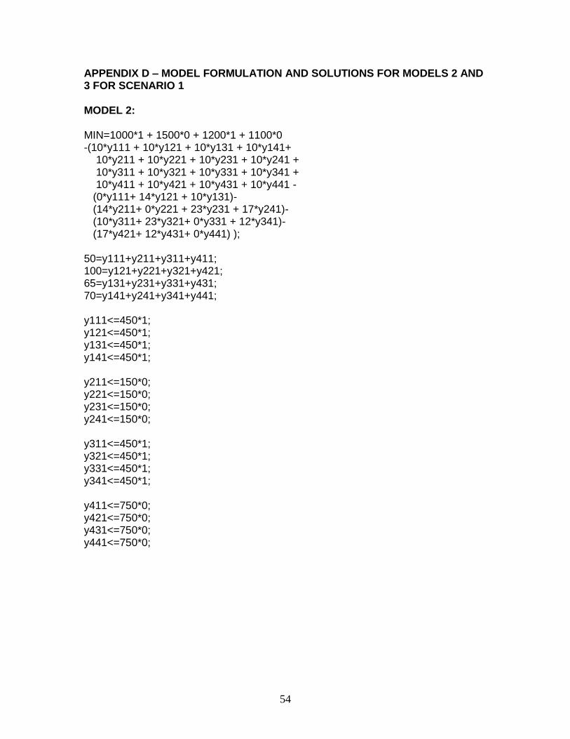
54
APPENDIX D – MODEL FORMULATION AND SOLUTIONS FOR MODELS 2 AND 3 FOR SCENARIO 1 MODEL 2: MIN=1000*1 + 1500*0 + 1200*1 + 1100*0 -(10*y111 + 10*y121 + 10*y131 + 10*y141+ 10*y211 + 10*y221 + 10*y231 + 10*y241 + 10*y311 + 10*y321 + 10*y331 + 10*y341 + 10*y411 + 10*y421 + 10*y431 + 10*y441 - (0*y111+ 14*y121 + 10*y131)- (14*y211+ 0*y221 + 23*y231 + 17*y241)- (10*y311+ 23*y321+ 0*y331 + 12*y341)- (17*y421+ 12*y431+ 0*y441) ); 50=y111+y211+y311+y411; 100=y121+y221+y321+y421; 65=y131+y231+y331+y431; 70=y141+y241+y341+y441; y111<=450*1; y121<=450*1; y131<=450*1; y141<=450*1; y211<=150*0; y221<=150*0; y231<=150*0; y241<=150*0; y311<=450*1; y321<=450*1; y331<=450*1; y341<=450*1; y411<=750*0; y421<=750*0; y431<=750*0; y441<=750*0;

55
MODEL 2 SOLUTION: Rows= 21 Vars= 16 No. integer vars= 0 ( all are linear) Nonzeros= 59 Constraint nonz= 32( 32 are +- 1) Density=0.165 Smallest and largest elements in abs value= 1.00000 450.000 No. < : 16 No. =: 4 No. > : 0, Obj=MIN, GUBs <= 16 Single cols= 0 Optimal solution found at step: 5 Objective value: 750.0000 Variable Value Reduced Cost Y111 50.00000 0.0000000 Y121 100.0000 0.0000000 Y131 0.0000000 10.00000 Y141 70.00000 0.0000000 Y211 0.0000000 14.00000 Y221 0.0000000 0.0000000 Y231 0.0000000 23.00000 Y241 0.0000000 17.00000 Y311 0.0000000 10.00000 Y321 0.0000000 9.000000 Y331 65.00000 0.0000000 Y341 0.0000000 12.00000 Y411 0.0000000 0.0000000 Y421 0.0000000 3.000000 Y431 0.0000000 12.00000 Y441 0.0000000 0.0000000 Row Slack or Surplus Dual Price 1 750.0000 1.000000 2 0.0000000 -10.00000 3 0.0000000 4.000000 4 0.0000000 -10.00000 5 0.0000000 -10.00000 6 400.0000 0.0000000 7 350.0000 0.0000000 8 450.0000 0.0000000 9 380.0000 0.0000000 10 0.0000000 0.0000000 11 0.0000000 14.00000 12 0.0000000 0.0000000 13 0.0000000 0.0000000 14 450.0000 0.0000000 15 450.0000 0.0000000 16 385.0000 0.0000000
56
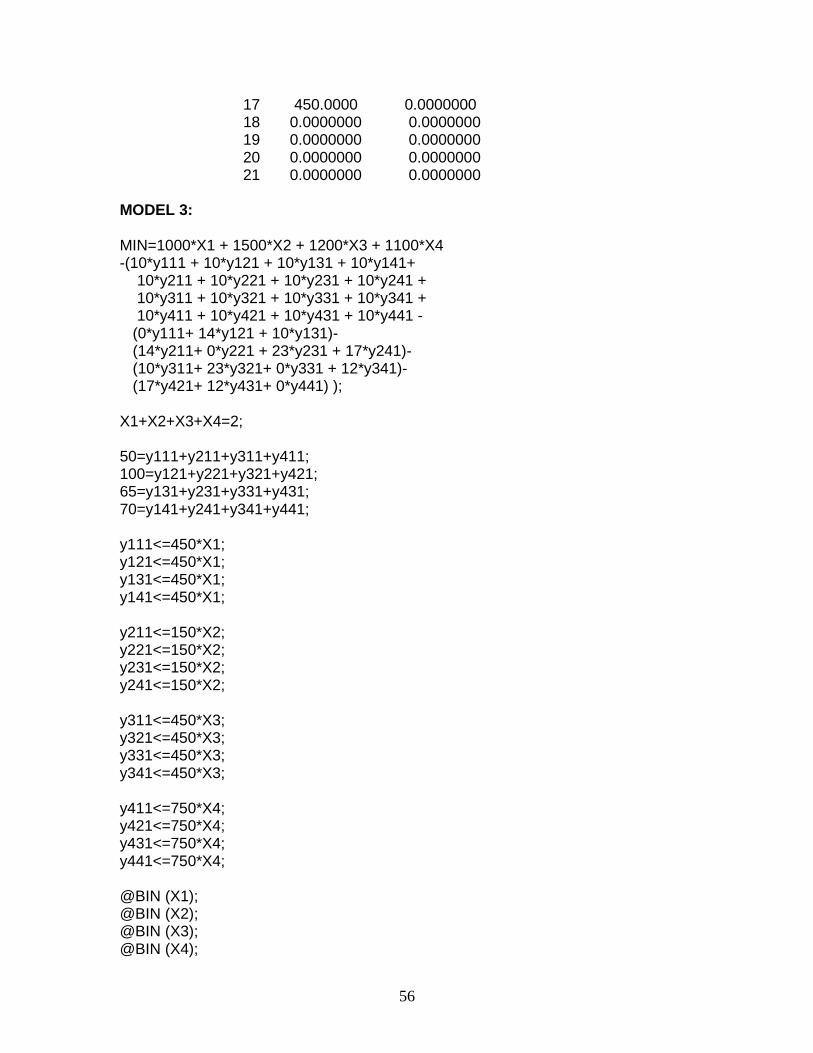
17 450.0000 0.0000000 18 0.0000000 0.0000000 19 0.0000000 0.0000000 20 0.0000000 0.0000000 21 0.0000000 0.0000000 MODEL 3:
MIN=1000*X1 + 1500*X2 + 1200*X3 + 1100*X4 -(10*y111 + 10*y121 + 10*y131 + 10*y141+ 10*y211 + 10*y221 + 10*y231 + 10*y241 + 10*y311 + 10*y321 + 10*y331 + 10*y341 + 10*y411 + 10*y421 + 10*y431 + 10*y441 - (0*y111+ 14*y121 + 10*y131)- (14*y211+ 0*y221 + 23*y231 + 17*y241)- (10*y311+ 23*y321+ 0*y331 + 12*y341)- (17*y421+ 12*y431+ 0*y441) ); X1+X2+X3+X4=2; 50=y111+y211+y311+y411; 100=y121+y221+y321+y421; 65=y131+y231+y331+y431; 70=y141+y241+y341+y441; y111<=450*X1; y121<=450*X1; y131<=450*X1; y141<=450*X1; y211<=150*X2; y221<=150*X2; y231<=150*X2; y241<=150*X2; y311<=450*X3; y321<=450*X3; y331<=450*X3; y341<=450*X3; y411<=750*X4; y421<=750*X4; y431<=750*X4; y441<=750*X4; @BIN (X1); @BIN (X2); @BIN (X3); @BIN (X4);

57
MODEL 3 SOLUTION: Rows= 22 Vars= 20 No. integer vars= 4 ( all are linear) Nonzeros= 75 Constraint nonz= 52( 36 are +- 1) Density=0.162 Smallest and largest elements in abs value= 1.00000 1500.00 No. < : 16 No. =: 5 No. > : 0, Obj=MIN, GUBs <= 7 Single cols= 0 Optimal solution found at step: 48 Objective value: 300.0000 Branch count: 4 Variable Value Reduced Cost X1 1.000000 1000.000 X2 1.000000 1500.000 X3 0.0000000 -3300.000 X4 0.0000000 1100.000 Y111 50.00000 0.0000000 Y121 0.0000000 14.00000 Y131 65.00000 0.0000000 Y141 70.00000 0.0000000 Y211 0.0000000 14.00000 Y221 100.0000 0.0000000 Y231 0.0000000 13.00000 Y241 0.0000000 17.00000 Y311 0.0000000 10.00000 Y321 0.0000000 23.00000 Y331 0.0000000 0.0000000 Y341 0.0000000 12.00000 Y411 0.0000000 0.0000000 Y421 0.0000000 17.00000 Y431 0.0000000 2.000000 Y441 0.0000000 0.0000000 Row Slack or Surplus Dual Price 1 300.0000 1.000000 2 0.0000000 0.0000000 3 0.0000000 -10.00000 4 0.0000000 -10.00000 5 0.0000000 0.0000000 6 0.0000000 -10.00000 7 400.0000 0.0000000 8 450.0000 0.0000000 9 385.0000 0.0000000 10 380.0000 0.0000000 11 150.0000 0.0000000 12 50.00000 0.0000000

58
13 150.0000 0.0000000 14 150.0000 0.0000000 15 0.0000000 0.0000000 16 0.0000000 0.0000000 17 0.0000000 10.00000 18 0.0000000 0.0000000 19 0.0000000 0.0000000 20 0.0000000 0.0000000 21 0.0000000 0.0000000 22 0.0000000 0.0000000

59
APPENDIX E – MODEL FORMULATION AND SOLUTIONS FOR MODELS 2 AND 3 FOR SCENARIO 2 MODEL 2: MIN=1000*1 + 1500*0 + 1200*1 + 1100*0 -(10*y112 + 10*y122 + 10*y132 + 10*y142+ 10*y212 + 10*y222 + 10*y232 + 10*y242+ 10*y312 + 10*y322 + 10*y332 + 10*y342+ 10*y412 + 10*y422 + 10*y432 + 10*y442- (0*y112+ 14*y122 + 10*y132)- (14*y212+ 0*y222 + 23*y232 + 17*y242)- (10*y312+ 23*y322+ 0*y332 + 12*y342)- (17*y422+ 12*y432+ 0*y442) ); 125=y112+y212+y312+y412; 300=y122+y222+y322+y422; 250=y132+y232+y332+y432; 175=y142+y242+y342+y442; y112<=450*1; y122<=450*1; y132<=450*1; y142<=450*1; y212<=150*0; y222<=150*0; y232<=150*0; y242<=150*0; y312<=450*1; y322<=450*1; y332<=450*1; y342<=450*1; y412<=750*0; y422<=750*0; y432<=750*0; y442<=750*0;
60
MODEL 2 SOLUTION: Rows= 21 Vars= 16 No. integer vars= 0 ( all are linear) Nonzeros= 59 Constraint nonz= 32( 32 are +- 1) Density=0.165 Smallest and largest elements in abs value= 1.00000 450.000 No. < : 16 No. =: 4 No. > : 0, Obj=MIN, GUBs <= 16 Single cols= 0 Optimal solution found at step: 5 Objective value: -2100.000 Variable Value Reduced Cost Y112 125.0000 0.0000000 Y122 300.0000 0.0000000 Y132 0.0000000 10.00000 Y142 175.0000 0.0000000 Y212 0.0000000 14.00000 Y222 0.0000000 0.0000000 Y232 0.0000000 23.00000 Y242 0.0000000 17.00000 Y312 0.0000000 10.00000 Y322 0.0000000 9.000000 Y332 250.0000 0.0000000 Y342 0.0000000 12.00000 Y412 0.0000000 0.0000000 Y422 0.0000000 3.000000 Y432 0.0000000 12.00000 Y442 0.0000000 0.0000000 Row Slack or Surplus Dual Price 1 -2100.000 1.000000 2 0.0000000 -10.00000 3 0.0000000 4.000000 4 0.0000000 -10.00000 5 0.0000000 -10.00000 6 325.0000 0.0000000 7 150.0000 0.0000000 8 450.0000 0.0000000 9 275.0000 0.0000000 10 0.0000000 0.0000000 11 0.0000000 14.00000 12 0.0000000 0.0000000 13 0.0000000 0.0000000 14 450.0000 0.0000000 15 450.0000 0.0000000 16 200.0000 0.0000000 17 450.0000 0.0000000 18 0.0000000 0.0000000 19 0.0000000 0.0000000
61
20 0.0000000 0.0000000 21 0.0000000 0.0000000 MODEL 3 MIN=1000*X1 + 1500*X2 + 1200*X3 + 1100*X4 -(10*y112 + 10*y122 + 10*y132 + 10*y142+ 10*y212 + 10*y222 + 10*y232 + 10*y242+ 10*y312 + 10*y322 + 10*y332 + 10*y342+ 10*y412 + 10*y422 + 10*y432 + 10*y442- (0*y112+ 14*y122 + 10*y132)- (14*y212+ 0*y222 + 23*y232 + 17*y242)- (10*y312+ 23*y322+ 0*y332 + 12*y342)- (17*y422+ 12*y432+ 0*y442) ); X1+X2+X3+X4=2; 125=y112+y212+y312+y412; 300=y122+y222+y322+y422; 250=y132+y232+y332+y432; 175=y142+y242+y342+y442; y112<=450*X1; y122<=450*X1; y132<=450*X1; y142<=450*X1; y212<=150*X2; y222<=150*X2; y232<=150*X2; y242<=150*X2; y312<=450*X3; y322<=450*X3; y332<=450*X3; y342<=450*X3; y412<=750*X4; y422<=750*X4; y432<=750*X4; y442<=750*X4; @BIN (X1); @BIN (X2); @BIN (X3); @BIN (X4);

62
MODEL 3 SOLUTION: Rows= 22 Vars= 20 No. integer vars= 4 ( all are linear) Nonzeros= 75 Constraint nonz= 52( 36 are +- 1) Density=0.162 Smallest and largest elements in abs value= 1.00000 1500.00 No. < : 16 No. =: 5 No. > : 0, Obj=MIN, GUBs <= 7 Single cols= 0 Optimal solution found at step: 30 Objective value: -2100.000 Branch count: 1 Variable Value Reduced Cost X1 1.000000 1000.000 X2 0.0000000 -600.0000 X3 1.000000 1200.000 X4 0.0000000 1100.000 Y112 125.0000 0.0000000 Y122 300.0000 0.0000000 Y132 0.0000000 10.00000 Y142 175.0000 0.0000000 Y212 0.0000000 14.00000 Y222 0.0000000 0.0000000 Y232 0.0000000 23.00000 Y242 0.0000000 17.00000 Y312 0.0000000 10.00000 Y322 0.0000000 9.000000 Y332 250.0000 0.0000000 Y342 0.0000000 12.00000 Y412 0.0000000 0.0000000 Y422 0.0000000 3.000000 Y432 0.0000000 12.00000 Y442 0.0000000 0.0000000 Row Slack or Surplus Dual Price 1 -2100.000 1.000000 2 0.0000000 0.0000000 3 0.0000000 -10.00000 4 0.0000000 4.000000 5 0.0000000 -10.00000 6 0.0000000 -10.00000 7 325.0000 0.0000000 8 150.0000 0.0000000 9 450.0000 0.0000000 10 275.0000 0.0000000 11 0.0000000 0.0000000 12 0.0000000 14.00000 13 0.0000000 0.0000000 14 0.0000000 0.0000000

63
15 450.0000 0.0000000 16 450.0000 0.0000000 17 200.0000 0.0000000 18 450.0000 0.0000000 19 0.0000000 0.0000000 20 0.0000000 0.0000000 21 0.0000000 0.0000000 22 0.0000000 0.0000000

64
APPENDIX F – MODEL FORMULATION AND SOLUTIONS FOR MODELS 2 AND 3 FOR SCENARIO 3 MODEL 2: MIN=1000*1 + 1500*0 + 1200*1 + 1100*0 -(10*y113 + 10*y123 + 10*y133 + 10*y143 + 10*y213 + 10*y223 + 10*y233 + 10*y243 + 10*y313 + 10*y323 + 10*y333 + 10*y343 + 10*y413 + 10*y423 + 10*y433 + 10*y443 - (0*y113+ 14*y123 + 10*y133)- (14*y213+ 0*y223 + 23*y233 + 17*y243)- (10*y313+ 23*y323+ 0*y333 + 12*y343)- (17*y423+ 12*y433+ 0*y443) ); 800=y113+y213+y313+y413; 750=y123+y223+y323+y423; 255=y133+y233+y333+y433; 810=y143+y243+y343+y443; y113<=450*1; y123<=450*1; y133<=450*1; y143<=450*1; y213<=150*0; y223<=150*0; y233<=150*0; y243<=150*0; y313<=450*1; y323<=450*1; y333<=450*1; y343<=450*1; y413<=750*0; y423<=750*0; y433<=750*0; y443<=750*0; MODEL 2 SOLUTION: Rows= 21 Vars= 16 No. integer vars= 0 ( all are linear) Nonzeros= 59 Constraint nonz= 32( 32 are +- 1) Density=0.165 Smallest and largest elements in abs value= 1.00000 810.000 No. < : 16 No. =: 4 No. > : 0, Obj=MIN, GUBs <= 16 Single cols= 0 Optimal solution found at step: 5

65
Objective value: -2930.000 Variable Value Reduced Cost Y113 450.0000 0.0000000 Y123 450.0000 0.0000000 Y133 0.0000000 10.00000 Y143 450.0000 0.0000000 Y213 0.0000000 4.000000 Y223 0.0000000 0.0000000 Y233 0.0000000 23.00000 Y243 0.0000000 5.000000 Y313 350.0000 0.0000000 Y323 300.0000 0.0000000 Y333 255.0000 0.0000000 Y343 360.0000 0.0000000 Y413 0.0000000 0.0000000 Y423 0.0000000 0.0000000 Y433 0.0000000 12.00000 Y443 0.0000000 0.0000000 Row Slack or Surplus Dual Price 1 -2930.000 1.000000 2 0.0000000 0.0000000 3 0.0000000 13.00000 4 0.0000000 -10.00000 5 0.0000000 2.000000 6 0.0000000 10.00000 7 0.0000000 9.000000 8 450.0000 0.0000000 9 0.0000000 12.00000 10 0.0000000 0.0000000 11 0.0000000 23.00000 12 0.0000000 0.0000000 13 0.0000000 0.0000000 14 100.0000 0.0000000 15 150.0000 0.0000000 16 195.0000 0.0000000 17 90.00000 0.0000000 18 0.0000000 10.00000 19 0.0000000 6.000000 20 0.0000000 0.0000000 21 0.0000000 12.00000

66
MODEL 3: MIN=1000*X1 + 1500*X2 + 1200*X3 + 1100*X4 -(10*y113 + 10*y123 + 10*y133 + 10*y143 + 10*y213 + 10*y223 + 10*y233 + 10*y243 + 10*y313 + 10*y323 + 10*y333 + 10*y343 + 10*y413 + 10*y423 + 10*y433 + 10*y443 - (0*y113+ 14*y123 + 10*y133)- (14*y213+ 0*y223 + 23*y233 + 17*y243)- (10*y313+ 23*y323+ 0*y333 + 12*y343)- (17*y423+ 12*y433+ 0*y443) ); X1+X2+X3+X4=2; 800=y113+y213+y313+y413; 750=y123+y223+y323+y423; 255=y133+y233+y333+y433; 810=y143+y243+y343+y443; y113<=450*X1; y123<=450*X1; y133<=450*X1; y143<=450*X1; y213<=150*X2; y223<=150*X2; y233<=150*X2; y243<=150*X2; y313<=450*X3; y323<=450*X3; y333<=450*X3; y343<=450*X3; y413<=750*X4; y423<=750*X4; y433<=750*X4; y443<=750*X4; @BIN (X1); @BIN (X2); @BIN (X3); @BIN (X4);

67
MODEL 3 SOLUTION: Rows= 22 Vars= 20 No. integer vars= 4 ( all are linear) Nonzeros= 75 Constraint nonz= 52( 36 are +- 1) Density=0.162 Smallest and largest elements in abs value= 1.00000 1500.00 No. < : 16 No. =: 5 No. > : 0, Obj=MIN, GUBs <= 7 Single cols= 0 Optimal solution found at step: 55 Objective value: -10100.00 Branch count: 3 Variable Value Reduced Cost X1 1.000000 -350.0000 X2 0.0000000 -1050.000 X3 0.0000000 -3300.000 X4 1.000000 1100.000 Y113 450.0000 0.0000000 Y123 450.0000 0.0000000 Y133 255.0000 0.0000000 Y143 450.0000 0.0000000 Y213 0.0000000 14.00000 Y223 0.0000000 0.0000000 Y233 0.0000000 13.00000 Y243 0.0000000 17.00000 Y313 0.0000000 10.00000 Y323 0.0000000 6.000000 Y333 0.0000000 0.0000000 Y343 0.0000000 12.00000 Y413 350.0000 0.0000000 Y423 300.0000 0.0000000 Y433 0.0000000 2.000000 Y443 360.0000 0.0000000 Row Slack or Surplus Dual Price 1 -10100.00 1.000000 2 0.0000000 0.0000000 3 0.0000000 -10.00000 4 0.0000000 7.000000 5 0.0000000 0.0000000 6 0.0000000 -10.00000 7 0.0000000 0.0000000 8 0.0000000 3.000000 9 195.0000 0.0000000 10 0.0000000 0.0000000 11 0.0000000 0.0000000 12 0.0000000 17.00000 13 0.0000000 0.0000000 14 0.0000000 0.0000000 15 0.0000000 0.0000000

68
16 0.0000000 0.0000000 17 0.0000000 10.00000 18 0.0000000 0.0000000 19 400.0000 0.0000000 20 450.0000 0.0000000 21 750.0000 0.0000000 22 390.0000 0.0000000

69
APPENDIX G – MODEL AND SOLUTIONS FOR DEMAND VARIANCE SCENARIO A (VARS1=8.54, VARS2=26.19, VARS3=69.40) MODEL 1: MIN=1000*X1 + 1500*X2 + 1200*X3 + 1100*X4 -(10*y111 + 10*y121 + 10*y131 + 10*y141+ 10*y211 + 10*y221 + 10*y231 + 10*y241 + 10*y311 + 10*y321 + 10*y331 + 10*y341 + 10*y411 + 10*y421 + 10*y431 + 10*y441 - (0*y111+ 14*y121 + 10*y131)- (14*y211+ 0*y221 + 23*y231 + 17*y241)- (10*y311+ 23*y321+ 0*y331 + 12*y341)- (17*y421+ 12*y431+ 0*y441) ) ; X1+X2+X3+X4=2; 312=y111+y211+y311+y411; 320=y121+y221+y321+y421; 284=y131+y231+y331+y431; 334=y141+y241+y341+y441; y111<=450*X1; y121<=450*X1; y131<=450*X1; y141<=450*X1; y211<=150*X2; y221<=150*X2; y231<=150*X2; y241<=150*X2; y311<=450*X3; y321<=450*X3; y331<=450*X3; y341<=450*X3; y411<=750*X4; y421<=750*X4; y431<=750*X4; y441<=750*X4; @BIN (X1); @BIN (X2); @BIN (X3); @BIN (X4);

70
MODEL 1 SOLUTION: Rows= 22 Vars= 20 No. integer vars= 4 ( all are linear) Nonzeros= 75 Constraint nonz= 52( 36 are +- 1) Density=0.162 Smallest and largest elements in abs value= 1.00000 1500.00 No. < : 16 No. =: 5 No. > : 0, Obj=MIN, GUBs <= 7 Single cols= 0 Optimal solution found at step: 29 Objective value: -5820.000 Branch count: 1 Variable Value Reduced Cost X1 1.000000 1000.000 X2 0.0000000 -600.0000 X3 1.000000 1200.000 X4 0.0000000 1100.000 Y111 312.0000 0.0000000 Y121 320.0000 0.0000000 Y131 0.0000000 10.00000 Y141 334.0000 0.0000000 Y211 0.0000000 14.00000 Y221 0.0000000 0.0000000 Y231 0.0000000 23.00000 Y241 0.0000000 17.00000 Y311 0.0000000 10.00000 Y321 0.0000000 9.000000 Y331 284.0000 0.0000000 Y341 0.0000000 12.00000 Y411 0.0000000 0.0000000 Y421 0.0000000 3.000000 Y431 0.0000000 12.00000 Y441 0.0000000 0.0000000 Row Slack or Surplus Dual Price 1 -5820.000 1.000000 2 0.0000000 0.0000000 3 0.0000000 -10.00000 4 0.0000000 4.000000 5 0.0000000 -10.00000 6 0.0000000 -10.00000 7 138.0000 0.0000000 8 130.0000 0.0000000 9 450.0000 0.0000000 10 116.0000 0.0000000 11 0.0000000 0.0000000 12 0.0000000 14.00000

71
13 0.0000000 0.0000000 14 0.0000000 0.0000000 15 450.0000 0.0000000 16 450.0000 0.0000000 17 166.0000 0.0000000 18 450.0000 0.0000000 19 0.0000000 0.0000000 20 0.0000000 0.0000000 21 0.0000000 0.0000000 22 0.0000000 0.0000000 MODEL 2: MIN=1000*1 + 1500*0 + 1200*1 + 1100*0 -1/3*(10*y111 + 10*y121 + 10*y131 + 10*y141+ 10*y211 + 10*y221 + 10*y231 + 10*y241 + 10*y311 + 10*y321 + 10*y331 + 10*y341 + 10*y411 + 10*y421 + 10*y431 + 10*y441 - (0*y111+ 14*y121 + 10*y131)- (14*y211+ 0*y221 + 23*y231 + 17*y241)- (10*y311+ 23*y321+ 0*y331 + 12*y341)- (17*y421+ 12*y431+ 0*y441) ) -1/3*(10*y112 + 10*y122 + 10*y132 + 10*y142+ 10*y212 + 10*y222 + 10*y232 + 10*y242+ 10*y312 + 10*y322 + 10*y332 + 10*y342+ 10*y412 + 10*y422 + 10*y432 + 10*y442- (0*y112+ 14*y122 + 10*y132)- (14*y212+ 0*y222 + 23*y232 + 17*y242)- (10*y312+ 23*y322+ 0*y332 + 12*y342)- (17*y422+ 12*y432+ 0*y442) ) -1/3*(10*y113 + 10*y123 + 10*y133 + 10*y143 + 10*y213 + 10*y223 + 10*y233 + 10*y243 + 10*y313 + 10*y323 + 10*y333 + 10*y343 + 10*y413 + 10*y423 + 10*y433 + 10*y443 - (0*y113+ 14*y123 + 10*y133)- (14*y213+ 0*y223 + 23*y233 + 17*y243)- (10*y313+ 23*y323+ 0*y333 + 12*y343)- (17*y423+ 12*y433+ 0*y443) ); 60=y111+y211+y311+y411; 175=y112+y212+y312+y412; 701=y113+y213+y313+y413; 80=y121+y221+y321+y421; 235=y122+y222+y322+y422; 645=y123+y223+y323+y423;

72
70=y131+y231+y331+y431; 224=y132+y232+y332+y432; 559=y133+y233+y333+y433; 75=y141+y241+y341+y441; 216=y142+y242+y342+y442; 710=y143+y243+y343+y443; y111<=450*1; y121<=450*1; y131<=450*1; y141<=450*1; y112<=450*1; y122<=450*1; y132<=450*1; y142<=450*1; y113<=450*1; y123<=450*1; y133<=450*1; y143<=450*1; y211<=150*0; y221<=150*0; y231<=150*0; y241<=150*0; y212<=150*0; y222<=150*0; y232<=150*0; y242<=150*0; y213<=150*0; y223<=150*0; y233<=150*0; y243<=150*0; y311<=450*1; y321<=450*1; y331<=450*1; y341<=450*1; y312<=450*1; y322<=450*1; y332<=450*1; y342<=450*1;
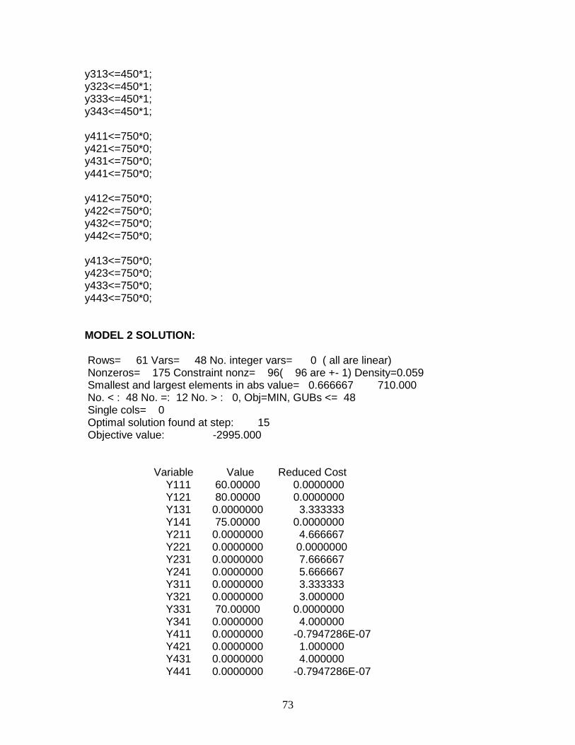
73
y313<=450*1; y323<=450*1; y333<=450*1; y343<=450*1; y411<=750*0; y421<=750*0; y431<=750*0; y441<=750*0; y412<=750*0; y422<=750*0; y432<=750*0; y442<=750*0; y413<=750*0; y423<=750*0; y433<=750*0; y443<=750*0; MODEL 2 SOLUTION: Rows= 61 Vars= 48 No. integer vars= 0 ( all are linear) Nonzeros= 175 Constraint nonz= 96( 96 are +- 1) Density=0.059 Smallest and largest elements in abs value= 0.666667 710.000 No. < : 48 No. =: 12 No. > : 0, Obj=MIN, GUBs <= 48 Single cols= 0 Optimal solution found at step: 15 Objective value: -2995.000 Variable Value Reduced Cost Y111 60.00000 0.0000000 Y121 80.00000 0.0000000 Y131 0.0000000 3.333333 Y141 75.00000 0.0000000 Y211 0.0000000 4.666667 Y221 0.0000000 0.0000000 Y231 0.0000000 7.666667 Y241 0.0000000 5.666667 Y311 0.0000000 3.333333 Y321 0.0000000 3.000000 Y331 70.00000 0.0000000 Y341 0.0000000 4.000000 Y411 0.0000000 -0.7947286E-07 Y421 0.0000000 1.000000 Y431 0.0000000 4.000000 Y441 0.0000000 -0.7947286E-07
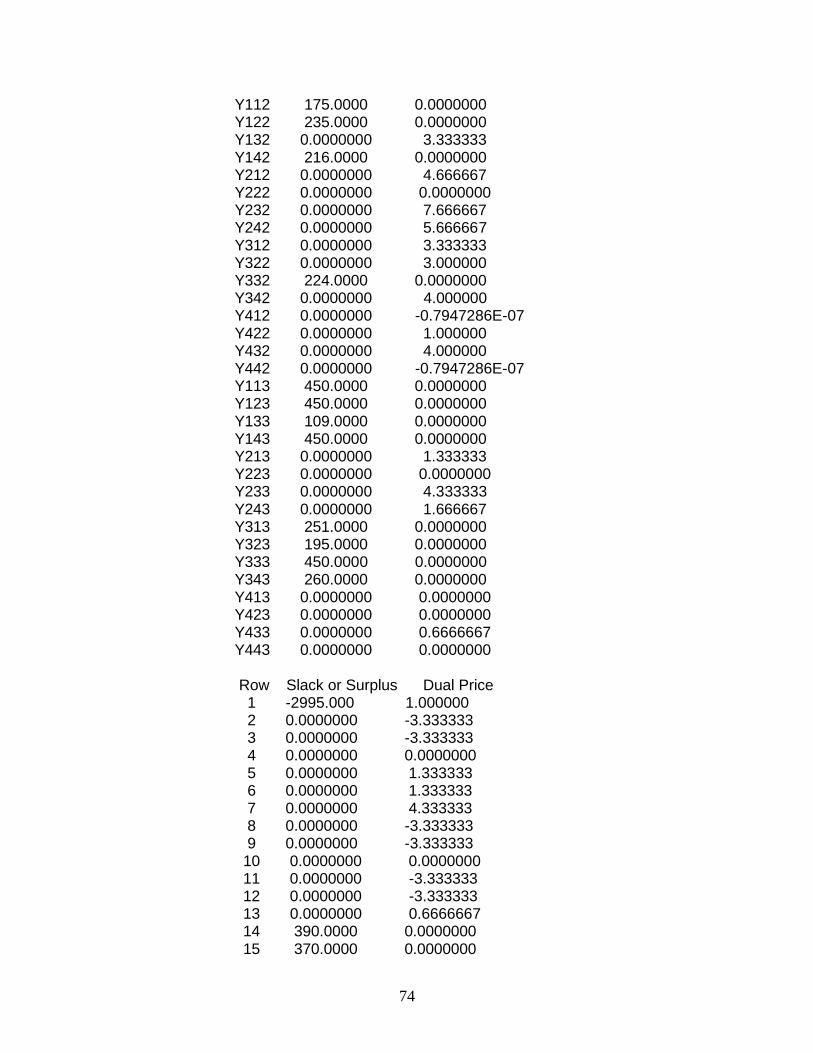
74
Y112 175.0000 0.0000000 Y122 235.0000 0.0000000 Y132 0.0000000 3.333333 Y142 216.0000 0.0000000 Y212 0.0000000 4.666667 Y222 0.0000000 0.0000000 Y232 0.0000000 7.666667 Y242 0.0000000 5.666667 Y312 0.0000000 3.333333 Y322 0.0000000 3.000000 Y332 224.0000 0.0000000 Y342 0.0000000 4.000000 Y412 0.0000000 -0.7947286E-07 Y422 0.0000000 1.000000 Y432 0.0000000 4.000000 Y442 0.0000000 -0.7947286E-07 Y113 450.0000 0.0000000 Y123 450.0000 0.0000000 Y133 109.0000 0.0000000 Y143 450.0000 0.0000000 Y213 0.0000000 1.333333 Y223 0.0000000 0.0000000 Y233 0.0000000 4.333333 Y243 0.0000000 1.666667 Y313 251.0000 0.0000000 Y323 195.0000 0.0000000 Y333 450.0000 0.0000000 Y343 260.0000 0.0000000 Y413 0.0000000 0.0000000 Y423 0.0000000 0.0000000 Y433 0.0000000 0.6666667 Y443 0.0000000 0.0000000 Row Slack or Surplus Dual Price 1 -2995.000 1.000000 2 0.0000000 -3.333333 3 0.0000000 -3.333333 4 0.0000000 0.0000000 5 0.0000000 1.333333 6 0.0000000 1.333333 7 0.0000000 4.333333 8 0.0000000 -3.333333 9 0.0000000 -3.333333 10 0.0000000 0.0000000 11 0.0000000 -3.333333 12 0.0000000 -3.333333 13 0.0000000 0.6666667 14 390.0000 0.0000000 15 370.0000 0.0000000

75
16 450.0000 0.0000000 17 375.0000 0.0000000 18 275.0000 0.0000000 19 215.0000 0.0000000 20 450.0000 0.0000000 21 234.0000 0.0000000 22 0.0000000 3.333333 23 0.0000000 3.000000 24 341.0000 0.0000000 25 0.0000000 4.000000 26 0.0000000 0.0000000 27 0.0000000 4.666667 28 0.0000000 0.0000000 29 0.0000000 0.0000000 30 0.0000000 0.0000000 31 0.0000000 4.666667 32 0.0000000 0.0000000 33 0.0000000 0.0000000 34 0.0000000 0.0000000 35 0.0000000 7.666667 36 0.0000000 0.0000000 37 0.0000000 0.0000000 38 450.0000 0.0000000 39 450.0000 0.0000000 40 380.0000 0.0000000 41 450.0000 0.0000000 42 450.0000 0.0000000 43 450.0000 0.0000000 44 226.0000 0.0000000 45 450.0000 0.0000000 46 199.0000 0.0000000 47 255.0000 0.0000000 48 0.0000000 3.333333 49 190.0000 0.0000000 50 0.0000000 0.0000000 51 0.0000000 0.0000000 52 0.0000000 0.0000000 53 0.0000000 0.0000000 54 0.0000000 0.0000000 55 0.0000000 0.0000000 56 0.0000000 0.0000000 57 0.0000000 0.0000000 58 0.0000000 3.333333 59 0.0000000 2.000000 60 0.0000000 0.0000000 61 0.0000000 4.000000

76
MODEL 3: MIN=1000*X1 + 1500*X2 + 1200*X3 + 1100*X4 -1/3*(10*y111 + 10*y121 + 10*y131 + 10*y141+ 10*y211 + 10*y221 + 10*y231 + 10*y241 + 10*y311 + 10*y321 + 10*y331 + 10*y341 + 10*y411 + 10*y421 + 10*y431 + 10*y441 - (0*y111+ 14*y121 + 10*y131)- (14*y211+ 0*y221 + 23*y231 + 17*y241)- (10*y311+ 23*y321+ 0*y331 + 12*y341)- (17*y421+ 12*y431+ 0*y441) ) -1/3*(10*y112 + 10*y122 + 10*y132 + 10*y142+ 10*y212 + 10*y222 + 10*y232 + 10*y242+ 10*y312 + 10*y322 + 10*y332 + 10*y342+ 10*y412 + 10*y422 + 10*y432 + 10*y442- (0*y112+ 14*y122 + 10*y132)- (14*y212+ 0*y222 + 23*y232 + 17*y242)- (10*y312+ 23*y322+ 0*y332 + 12*y342)- (17*y422+ 12*y432+ 0*y442) ) -1/3*(10*y113 + 10*y123 + 10*y133 + 10*y143 + 10*y213 + 10*y223 + 10*y233 + 10*y243 + 10*y313 + 10*y323 + 10*y333 + 10*y343 + 10*y413 + 10*y423 + 10*y433 + 10*y443 - (0*y113+ 14*y123 + 10*y133)- (14*y213+ 0*y223 + 23*y233 + 17*y243)- (10*y313+ 23*y323+ 0*y333 + 12*y343)- (17*y423+ 12*y433+ 0*y443) ); X1+X2+X3+X4=2; 60=y111+y211+y311+y411; 175=y112+y212+y312+y412; 701=y113+y213+y313+y413; 80=y121+y221+y321+y421; 235=y122+y222+y322+y422; 645=y123+y223+y323+y423; 70=y131+y231+y331+y431; 224=y132+y232+y332+y432; 559=y133+y233+y333+y433; 75=y141+y241+y341+y441; 216=y142+y242+y342+y442; 710=y143+y243+y343+y443;

77
y111<=450*X1; y121<=450*X1; y131<=450*X1; y141<=450*X1; y112<=450*X1; y122<=450*X1; y132<=450*X1; y142<=450*X1; y113<=450*X1; y123<=450*X1; y133<=450*X1; y143<=450*X1; y211<=150*X2; y221<=150*X2; y231<=150*X2; y241<=150*X2; y212<=150*X2; y222<=150*X2; y232<=150*X2; y242<=150*X2; y213<=150*X2; y223<=150*X2; y233<=150*X2; y243<=150*X2; y311<=450*X3; y321<=450*X3; y331<=450*X3; y341<=450*X3; y312<=450*X3; y322<=450*X3; y332<=450*X3; y342<=450*X3; y313<=450*X3; y323<=450*X3; y333<=450*X3; y343<=450*X3; y411<=750*X4; y421<=750*X4; y431<=750*X4; y441<=750*X4;
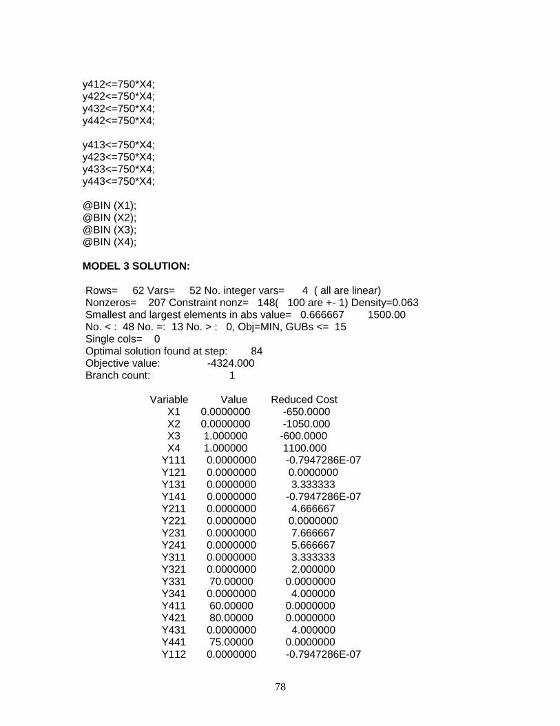
78
y412<=750*X4; y422<=750*X4; y432<=750*X4; y442<=750*X4; y413<=750*X4; y423<=750*X4; y433<=750*X4; y443<=750*X4; @BIN (X1); @BIN (X2); @BIN (X3); @BIN (X4); MODEL 3 SOLUTION: Rows= 62 Vars= 52 No. integer vars= 4 ( all are linear) Nonzeros= 207 Constraint nonz= 148( 100 are +- 1) Density=0.063 Smallest and largest elements in abs value= 0.666667 1500.00 No. < : 48 No. =: 13 No. > : 0, Obj=MIN, GUBs <= 15 Single cols= 0 Optimal solution found at step: 84 Objective value: -4324.000 Branch count: 1 Variable Value Reduced Cost X1 0.0000000 -650.0000 X2 0.0000000 -1050.000 X3 1.000000 -600.0000 X4 1.000000 1100.000 Y111 0.0000000 -0.7947286E-07 Y121 0.0000000 0.0000000 Y131 0.0000000 3.333333 Y141 0.0000000 -0.7947286E-07 Y211 0.0000000 4.666667 Y221 0.0000000 0.0000000 Y231 0.0000000 7.666667 Y241 0.0000000 5.666667 Y311 0.0000000 3.333333 Y321 0.0000000 2.000000 Y331 70.00000 0.0000000 Y341 0.0000000 4.000000 Y411 60.00000 0.0000000 Y421 80.00000 0.0000000 Y431 0.0000000 4.000000 Y441 75.00000 0.0000000 Y112 0.0000000 -0.7947286E-07

79
Y122 0.0000000 0.0000000 Y132 0.0000000 3.333333 Y142 0.0000000 -0.7947286E-07 Y212 0.0000000 4.666667 Y222 0.0000000 0.0000000 Y232 0.0000000 7.666667 Y242 0.0000000 5.666667 Y312 0.0000000 3.333333 Y322 0.0000000 2.000000 Y332 224.0000 0.0000000 Y342 0.0000000 4.000000 Y412 175.0000 0.0000000 Y422 235.0000 0.0000000 Y432 0.0000000 4.000000 Y442 216.0000 0.0000000 Y113 0.0000000 -0.7947286E-07 Y123 0.0000000 0.0000000 Y133 0.0000000 0.0000000 Y143 0.0000000 -0.7947286E-07 Y213 0.0000000 4.666667 Y223 0.0000000 0.0000000 Y233 0.0000000 3.666667 Y243 0.0000000 5.666667 Y313 0.0000000 3.333333 Y323 0.0000000 2.000000 Y333 450.0000 0.0000000 Y343 0.0000000 4.000000 Y413 701.0000 0.0000000 Y423 645.0000 0.0000000 Y433 109.0000 0.0000000 Y443 710.0000 0.0000000 Row Slack or Surplus Dual Price 1 -4324.000 1.000000 2 0.0000000 0.0000000 3 0.0000000 -3.333333 4 0.0000000 -3.333333 5 0.0000000 -3.333333 6 0.0000000 2.333333 7 0.0000000 2.333333 8 0.0000000 2.333333 9 0.0000000 -3.333333 10 0.0000000 -3.333333 11 0.0000000 0.6666667 12 0.0000000 -3.333333 13 0.0000000 -3.333333 14 0.0000000 -3.333333 15 0.0000000 0.0000000 16 0.0000000 1.000000

80
17 0.0000000 0.0000000 18 0.0000000 0.0000000 19 0.0000000 0.0000000 20 0.0000000 1.000000 21 0.0000000 0.0000000 22 0.0000000 0.0000000 23 0.0000000 0.0000000 24 0.0000000 1.000000 25 0.0000000 0.6666667 26 0.0000000 0.0000000 27 0.0000000 0.0000000 28 0.0000000 5.666667 29 0.0000000 0.0000000 30 0.0000000 0.0000000 31 0.0000000 0.0000000 32 0.0000000 5.666667 33 0.0000000 0.0000000 34 0.0000000 0.0000000 35 0.0000000 0.0000000 36 0.0000000 5.666667 37 0.0000000 0.0000000 38 0.0000000 0.0000000 39 450.0000 0.0000000 40 450.0000 0.0000000 41 380.0000 0.0000000 42 450.0000 0.0000000 43 450.0000 0.0000000 44 450.0000 0.0000000 45 226.0000 0.0000000 46 450.0000 0.0000000 47 450.0000 0.0000000 48 450.0000 0.0000000 49 0.0000000 4.000000 50 450.0000 0.0000000 51 690.0000 0.0000000 52 670.0000 0.0000000 53 750.0000 0.0000000 54 675.0000 0.0000000 55 575.0000 0.0000000 56 515.0000 0.0000000 57 750.0000 0.0000000 58 534.0000 0.0000000 59 49.00000 0.0000000 60 105.0000 0.0000000 61 641.0000 0.0000000 62 40.00000 0.0000000
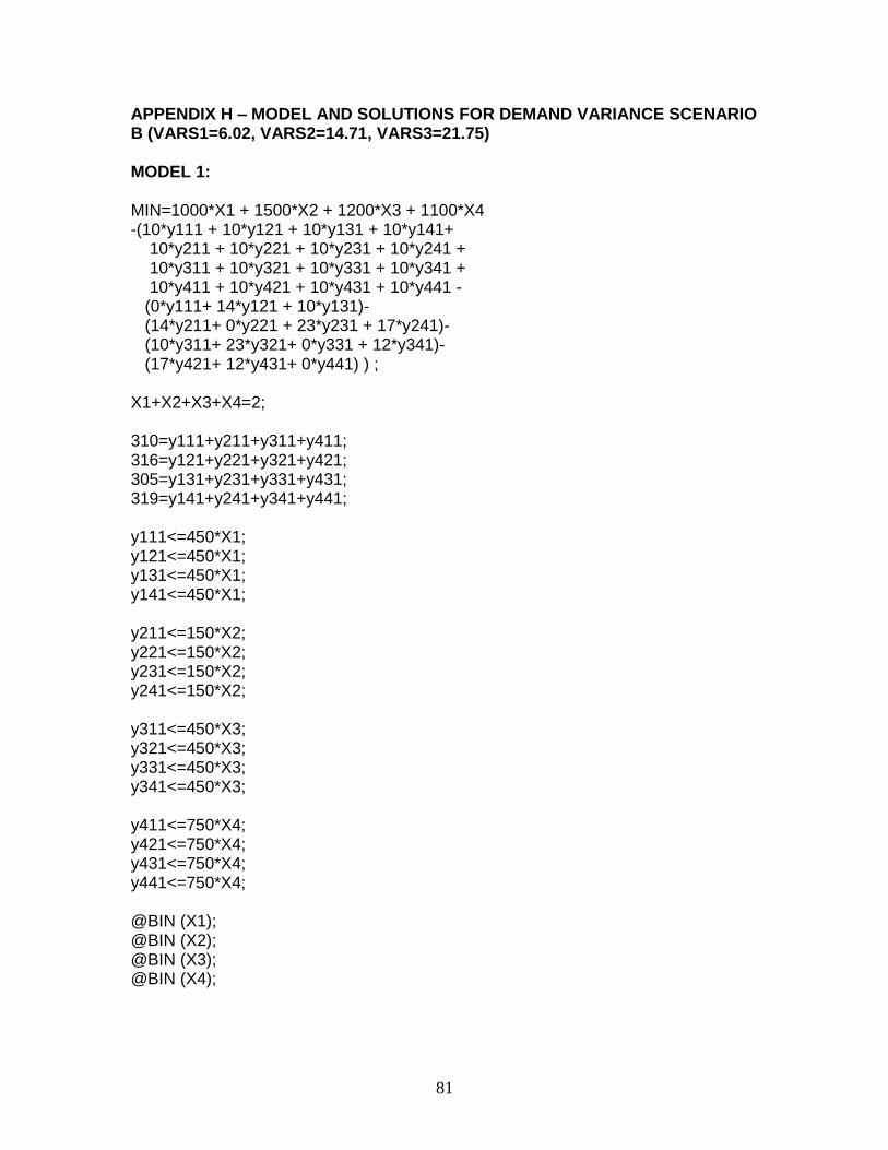
81
APPENDIX H – MODEL AND SOLUTIONS FOR DEMAND VARIANCE SCENARIO B (VARS1=6.02, VARS2=14.71, VARS3=21.75) MODEL 1: MIN=1000*X1 + 1500*X2 + 1200*X3 + 1100*X4 -(10*y111 + 10*y121 + 10*y131 + 10*y141+ 10*y211 + 10*y221 + 10*y231 + 10*y241 + 10*y311 + 10*y321 + 10*y331 + 10*y341 + 10*y411 + 10*y421 + 10*y431 + 10*y441 - (0*y111+ 14*y121 + 10*y131)- (14*y211+ 0*y221 + 23*y231 + 17*y241)- (10*y311+ 23*y321+ 0*y331 + 12*y341)- (17*y421+ 12*y431+ 0*y441) ) ; X1+X2+X3+X4=2; 310=y111+y211+y311+y411; 316=y121+y221+y321+y421; 305=y131+y231+y331+y431; 319=y141+y241+y341+y441; y111<=450*X1; y121<=450*X1; y131<=450*X1; y141<=450*X1; y211<=150*X2; y221<=150*X2; y231<=150*X2; y241<=150*X2; y311<=450*X3; y321<=450*X3; y331<=450*X3; y341<=450*X3; y411<=750*X4; y421<=750*X4; y431<=750*X4; y441<=750*X4; @BIN (X1); @BIN (X2); @BIN (X3); @BIN (X4);

82
MODEL 1 SOLUTION: Rows= 22 Vars= 20 No. integer vars= 4 ( all are linear) Nonzeros= 75 Constraint nonz= 52( 36 are +- 1) Density=0.162 Smallest and largest elements in abs value= 1.00000 1500.00 No. < : 16 No. =: 5 No. > : 0, Obj=MIN, GUBs <= 7 Single cols= 0 Optimal solution found at step: 32 Objective value: -5876.000 Branch count: 1 Variable Value Reduced Cost X1 1.000000 1000.000 X2 0.0000000 -600.0000 X3 1.000000 1200.000 X4 0.0000000 1100.000 Y111 310.0000 0.0000000 Y121 316.0000 0.0000000 Y131 0.0000000 10.00000 Y141 319.0000 0.0000000 Y211 0.0000000 14.00000 Y221 0.0000000 0.0000000 Y231 0.0000000 23.00000 Y241 0.0000000 17.00000 Y311 0.0000000 10.00000 Y321 0.0000000 9.000000 Y331 305.0000 0.0000000 Y341 0.0000000 12.00000 Y411 0.0000000 0.0000000 Y421 0.0000000 3.000000 Y431 0.0000000 12.00000 Y441 0.0000000 0.0000000 Row Slack or Surplus Dual Price 1 -5876.000 1.000000 2 0.0000000 0.0000000 3 0.0000000 -10.00000 4 0.0000000 4.000000 5 0.0000000 -10.00000 6 0.0000000 -10.00000 7 140.0000 0.0000000 8 134.0000 0.0000000 9 450.0000 0.0000000 10 131.0000 0.0000000 11 0.0000000 0.0000000 12 0.0000000 14.00000 13 0.0000000 0.0000000 14 0.0000000 0.0000000 15 450.0000 0.0000000 16 450.0000 0.0000000

83
17 145.0000 0.0000000 18 450.0000 0.0000000 19 0.0000000 0.0000000 20 0.0000000 0.0000000 21 0.0000000 0.0000000 22 0.0000000 0.0000000 MODEL 2: MIN=1000*1 + 1500*0 + 1200*1 + 1100*0 -1/3*(10*y111 + 10*y121 + 10*y131 + 10*y141+ 10*y211 + 10*y221 + 10*y231 + 10*y241 + 10*y311 + 10*y321 + 10*y331 + 10*y341 + 10*y411 + 10*y421 + 10*y431 + 10*y441 - (0*y111+ 14*y121 + 10*y131)- (14*y211+ 0*y221 + 23*y231 + 17*y241)- (10*y311+ 23*y321+ 0*y331 + 12*y341)- (17*y421+ 12*y431+ 0*y441) ) -1/3*(10*y112 + 10*y122 + 10*y132 + 10*y142+ 10*y212 + 10*y222 + 10*y232 + 10*y242+ 10*y312 + 10*y322 + 10*y332 + 10*y342+ 10*y412 + 10*y422 + 10*y432 + 10*y442- (0*y112+ 14*y122 + 10*y132)- (14*y212+ 0*y222 + 23*y232 + 17*y242)- (10*y312+ 23*y322+ 0*y332 + 12*y342)- (17*y422+ 12*y432+ 0*y442) ) -1/3*(10*y113 + 10*y123 + 10*y133 + 10*y143 + 10*y213 + 10*y223 + 10*y233 + 10*y243 + 10*y313 + 10*y323 + 10*y333 + 10*y343 + 10*y413 + 10*y423 + 10*y433 + 10*y443 - (0*y113+ 14*y123 + 10*y133)- (14*y213+ 0*y223 + 23*y233 + 17*y243)- (10*y313+ 23*y323+ 0*y333 + 12*y343)- (17*y423+ 12*y433+ 0*y443) ); 63=y111+y211+y311+y411; 191=y112+y212+y312+y412; 675=y113+y213+y313+y413; 74=y121+y221+y321+y421; 224=y122+y222+y322+y422; 650=y123+y223+y323+y423; 71=y131+y231+y331+y431; 219=y132+y232+y332+y432; 625=y133+y233+y333+y433;

84
77=y141+y241+y341+y441; 216=y142+y242+y342+y442; 665=y143+y243+y343+y443; y111<=450*1; y121<=450*1; y131<=450*1; y141<=450*1; y112<=450*1; y122<=450*1; y132<=450*1; y142<=450*1; y113<=450*1; y123<=450*1; y133<=450*1; y143<=450*1; y211<=150*0; y221<=150*0; y231<=150*0; y241<=150*0; y212<=150*0; y222<=150*0; y232<=150*0; y242<=150*0; y213<=150*0; y223<=150*0; y233<=150*0; y243<=150*0; y311<=450*1; y321<=450*1; y331<=450*1; y341<=450*1; y312<=450*1; y322<=450*1; y332<=450*1; y342<=450*1; y313<=450*1; y323<=450*1; y333<=450*1; y343<=450*1;

85
y411<=750*0; y421<=750*0; y431<=750*0; y441<=750*0; y412<=750*0; y422<=750*0; y432<=750*0; y442<=750*0; y413<=750*0; y423<=750*0; y433<=750*0; y443<=750*0; MODEL 2 SOLUTIONS: Rows= 61 Vars= 48 No. integer vars= 0 ( all are linear) Nonzeros= 175 Constraint nonz= 96( 96 are +- 1) Density=0.059 Smallest and largest elements in abs value= 0.666667 675.000 No. < : 48 No. =: 12 No. > : 0, Obj=MIN, GUBs <= 48 Single cols= 0 Optimal solution found at step: 15 Objective value: -3082.667 Variable Value Reduced Cost Y111 63.00000 0.0000000 Y121 74.00000 0.0000000 Y131 0.0000000 3.333333 Y141 77.00000 0.0000000 Y211 0.0000000 4.666667 Y221 0.0000000 0.0000000 Y231 0.0000000 7.666667 Y241 0.0000000 5.666667 Y311 0.0000000 3.333333 Y321 0.0000000 3.000000 Y331 71.00000 0.0000000 Y341 0.0000000 4.000000 Y411 0.0000000 -0.7947286E-07 Y421 0.0000000 1.000000 Y431 0.0000000 4.000000 Y441 0.0000000 -0.7947286E-07 Y112 191.0000 0.0000000 Y122 224.0000 0.0000000 Y132 0.0000000 3.333333 Y142 216.0000 0.0000000 Y212 0.0000000 4.666667

86
Y222 0.0000000 0.0000000 Y232 0.0000000 7.666667 Y242 0.0000000 5.666667 Y312 0.0000000 3.333333 Y322 0.0000000 3.000000 Y332 219.0000 0.0000000 Y342 0.0000000 4.000000 Y412 0.0000000 -0.7947286E-07 Y422 0.0000000 1.000000 Y432 0.0000000 4.000000 Y442 0.0000000 -0.7947286E-07 Y113 450.0000 0.0000000 Y123 450.0000 0.0000000 Y133 175.0000 0.0000000 Y143 450.0000 0.0000000 Y213 0.0000000 1.333333 Y223 0.0000000 0.0000000 Y233 0.0000000 4.333333 Y243 0.0000000 1.666667 Y313 225.0000 0.0000000 Y323 200.0000 0.0000000 Y333 450.0000 0.0000000 Y343 215.0000 0.0000000 Y413 0.0000000 0.0000000 Y423 0.0000000 0.0000000 Y433 0.0000000 0.6666667 Y443 0.0000000 0.0000000 Row Slack or Surplus Dual Price 1 -3082.667 1.000000 2 0.0000000 -3.333333 3 0.0000000 -3.333333 4 0.0000000 0.0000000 5 0.0000000 1.333333 6 0.0000000 1.333333 7 0.0000000 4.333333 8 0.0000000 -3.333333 9 0.0000000 -3.333333 10 0.0000000 0.0000000 11 0.0000000 -3.333333 12 0.0000000 -3.333333 13 0.0000000 0.6666667 14 387.0000 0.0000000 15 376.0000 0.0000000 16 450.0000 0.0000000 17 373.0000 0.0000000 18 259.0000 0.0000000 19 226.0000 0.0000000 20 450.0000 0.0000000
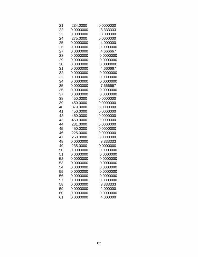
87
21 234.0000 0.0000000 22 0.0000000 3.333333 23 0.0000000 3.000000 24 275.0000 0.0000000 25 0.0000000 4.000000 26 0.0000000 0.0000000 27 0.0000000 4.666667 28 0.0000000 0.0000000 29 0.0000000 0.0000000 30 0.0000000 0.0000000 31 0.0000000 4.666667 32 0.0000000 0.0000000 33 0.0000000 0.0000000 34 0.0000000 0.0000000 35 0.0000000 7.666667 36 0.0000000 0.0000000 37 0.0000000 0.0000000 38 450.0000 0.0000000 39 450.0000 0.0000000 40 379.0000 0.0000000 41 450.0000 0.0000000 42 450.0000 0.0000000 43 450.0000 0.0000000 44 231.0000 0.0000000 45 450.0000 0.0000000 46 225.0000 0.0000000 47 250.0000 0.0000000 48 0.0000000 3.333333 49 235.0000 0.0000000 50 0.0000000 0.0000000 51 0.0000000 0.0000000 52 0.0000000 0.0000000 53 0.0000000 0.0000000 54 0.0000000 0.0000000 55 0.0000000 0.0000000 56 0.0000000 0.0000000 57 0.0000000 0.0000000 58 0.0000000 3.333333 59 0.0000000 2.000000 60 0.0000000 0.0000000 61 0.0000000 4.000000
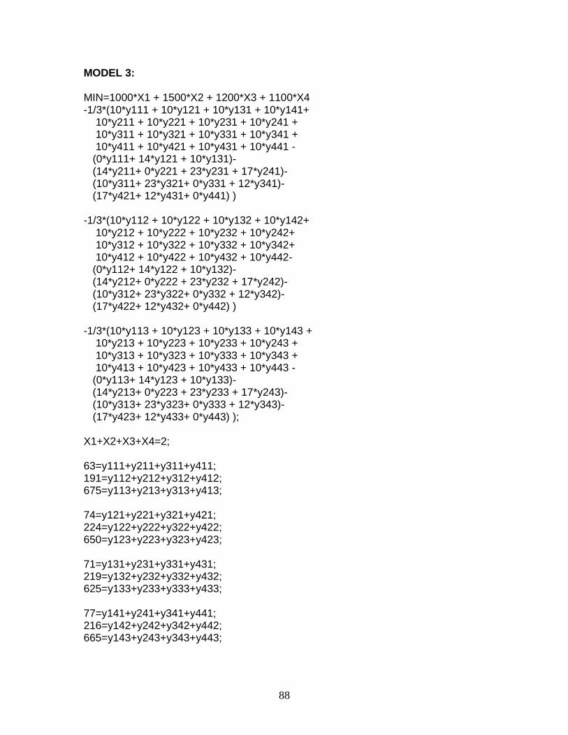
88
MODEL 3: MIN=1000*X1 + 1500*X2 + 1200*X3 + 1100*X4 -1/3*(10*y111 + 10*y121 + 10*y131 + 10*y141+ 10*y211 + 10*y221 + 10*y231 + 10*y241 + 10*y311 + 10*y321 + 10*y331 + 10*y341 + 10*y411 + 10*y421 + 10*y431 + 10*y441 - (0*y111+ 14*y121 + 10*y131)- (14*y211+ 0*y221 + 23*y231 + 17*y241)- (10*y311+ 23*y321+ 0*y331 + 12*y341)- (17*y421+ 12*y431+ 0*y441) ) -1/3*(10*y112 + 10*y122 + 10*y132 + 10*y142+ 10*y212 + 10*y222 + 10*y232 + 10*y242+ 10*y312 + 10*y322 + 10*y332 + 10*y342+ 10*y412 + 10*y422 + 10*y432 + 10*y442- (0*y112+ 14*y122 + 10*y132)- (14*y212+ 0*y222 + 23*y232 + 17*y242)- (10*y312+ 23*y322+ 0*y332 + 12*y342)- (17*y422+ 12*y432+ 0*y442) ) -1/3*(10*y113 + 10*y123 + 10*y133 + 10*y143 + 10*y213 + 10*y223 + 10*y233 + 10*y243 + 10*y313 + 10*y323 + 10*y333 + 10*y343 + 10*y413 + 10*y423 + 10*y433 + 10*y443 - (0*y113+ 14*y123 + 10*y133)- (14*y213+ 0*y223 + 23*y233 + 17*y243)- (10*y313+ 23*y323+ 0*y333 + 12*y343)- (17*y423+ 12*y433+ 0*y443) ); X1+X2+X3+X4=2; 63=y111+y211+y311+y411; 191=y112+y212+y312+y412; 675=y113+y213+y313+y413; 74=y121+y221+y321+y421; 224=y122+y222+y322+y422; 650=y123+y223+y323+y423; 71=y131+y231+y331+y431; 219=y132+y232+y332+y432; 625=y133+y233+y333+y433; 77=y141+y241+y341+y441; 216=y142+y242+y342+y442; 665=y143+y243+y343+y443;

89
y111<=450*X1; y121<=450*X1; y131<=450*X1; y141<=450*X1; y112<=450*X1; y122<=450*X1; y132<=450*X1; y142<=450*X1; y113<=450*X1; y123<=450*X1; y133<=450*X1; y143<=450*X1; y211<=150*X2; y221<=150*X2; y231<=150*X2; y241<=150*X2; y212<=150*X2; y222<=150*X2; y232<=150*X2; y242<=150*X2; y213<=150*X2; y223<=150*X2; y233<=150*X2; y243<=150*X2; y311<=450*X3; y321<=450*X3; y331<=450*X3; y341<=450*X3; y312<=450*X3; y322<=450*X3; y332<=450*X3; y342<=450*X3; y313<=450*X3; y323<=450*X3; y333<=450*X3; y343<=450*X3; y411<=750*X4; y421<=750*X4; y431<=750*X4; y441<=750*X4;

90
y412<=750*X4; y422<=750*X4; y432<=750*X4; y442<=750*X4; y413<=750*X4; y423<=750*X4; y433<=750*X4; y443<=750*X4; @BIN (X1); @BIN (X2); @BIN (X3); @BIN (X4); MODEL 3 SOLUTION: Rows= 62 Vars= 52 No. integer vars= 4 ( all are linear) Nonzeros= 207 Constraint nonz= 148( 100 are +- 1) Density=0.063 Smallest and largest elements in abs value= 0.666667 1500.00 No. < : 48 No. =: 13 No. > : 0, Obj=MIN, GUBs <= 15 Single cols= 0 Optimal solution found at step: 83 Objective value: -4128.000 Branch count: 1 Variable Value Reduced Cost X1 0.0000000 -650.0000 X2 0.0000000 -1050.000 X3 1.000000 -600.0000 X4 1.000000 1100.000 Y111 0.0000000 -0.7947286E-07 Y121 0.0000000 0.0000000 Y131 0.0000000 3.333333 Y141 0.0000000 -0.7947286E-07 Y211 0.0000000 4.666667 Y221 0.0000000 0.0000000 Y231 0.0000000 7.666667 Y241 0.0000000 5.666667 Y311 0.0000000 3.333333 Y321 0.0000000 2.000000 Y331 71.00000 0.0000000 Y341 0.0000000 4.000000 Y411 63.00000 0.0000000 Y421 74.00000 0.0000000

91
Y431 0.0000000 4.000000 Y441 77.00000 0.0000000 Y112 0.0000000 -0.7947286E-07 Y122 0.0000000 0.0000000 Y132 0.0000000 3.333333 Y142 0.0000000 -0.7947286E-07 Y212 0.0000000 4.666667 Y222 0.0000000 0.0000000 Y232 0.0000000 7.666667 Y242 0.0000000 5.666667 Y312 0.0000000 3.333333 Y322 0.0000000 2.000000 Y332 219.0000 0.0000000 Y342 0.0000000 4.000000 Y412 191.0000 0.0000000 Y422 224.0000 0.0000000 Y432 0.0000000 4.000000 Y442 216.0000 0.0000000 Y113 0.0000000 -0.7947286E-07 Y123 0.0000000 0.0000000 Y133 0.0000000 0.0000000 Y143 0.0000000 -0.7947286E-07 Y213 0.0000000 4.666667 Y223 0.0000000 0.0000000 Y233 0.0000000 3.666667 Y243 0.0000000 5.666667 Y313 0.0000000 3.333333 Y323 0.0000000 2.000000 Y333 450.0000 0.0000000 Y343 0.0000000 4.000000 Y413 675.0000 0.0000000 Y423 650.0000 0.0000000 Y433 175.0000 0.0000000 Y443 665.0000 0.0000000 Row Slack or Surplus Dual Price 1 -4128.000 1.000000 2 0.0000000 0.0000000 3 0.0000000 -3.333333 4 0.0000000 -3.333333 5 0.0000000 -3.333333 6 0.0000000 2.333333 7 0.0000000 2.333333 8 0.0000000 2.333333 9 0.0000000 -3.333333 10 0.0000000 -3.333333 11 0.0000000 0.6666667 12 0.0000000 -3.333333 13 0.0000000 -3.333333

92
14 0.0000000 -3.333333 15 0.0000000 0.0000000 16 0.0000000 1.000000 17 0.0000000 0.0000000 18 0.0000000 0.0000000 19 0.0000000 0.0000000 20 0.0000000 1.000000 21 0.0000000 0.0000000 22 0.0000000 0.0000000 23 0.0000000 0.0000000 24 0.0000000 1.000000 25 0.0000000 0.6666667 26 0.0000000 0.0000000 27 0.0000000 0.0000000 28 0.0000000 5.666667 29 0.0000000 0.0000000 30 0.0000000 0.0000000 31 0.0000000 0.0000000 32 0.0000000 5.666667 33 0.0000000 0.0000000 34 0.0000000 0.0000000 35 0.0000000 0.0000000 36 0.0000000 5.666667 37 0.0000000 0.0000000 38 0.0000000 0.0000000 39 450.0000 0.0000000 40 450.0000 0.0000000 41 379.0000 0.0000000 42 450.0000 0.0000000 43 450.0000 0.0000000 44 450.0000 0.0000000 45 231.0000 0.0000000 46 450.0000 0.0000000 47 450.0000 0.0000000 48 450.0000 0.0000000 49 0.0000000 4.000000 50 450.0000 0.0000000 51 687.0000 0.0000000 52 676.0000 0.0000000 53 750.0000 0.0000000 54 673.0000 0.0000000 55 559.0000 0.0000000 56 526.0000 0.0000000 57 750.0000 0.0000000 58 534.0000 0.0000000 59 75.00000 0.0000000 60 100.0000 0.0000000 61 575.0000 0.0000000 62 85.00000 0.0000000
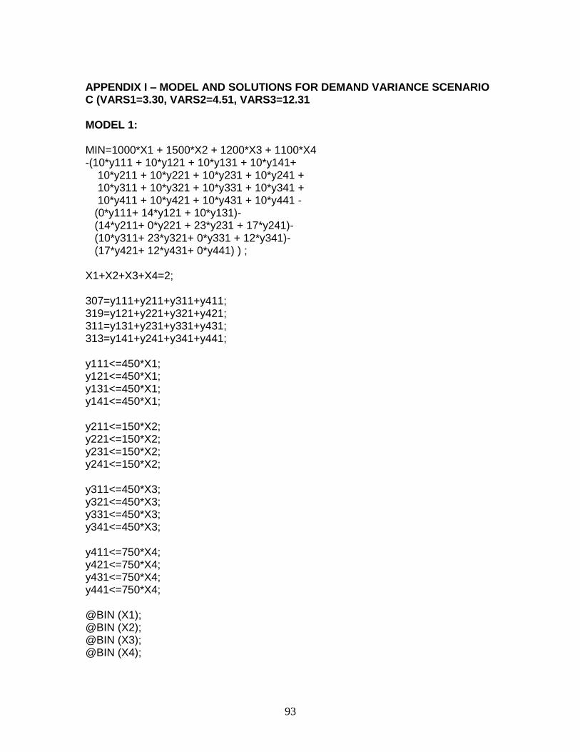
93
APPENDIX I – MODEL AND SOLUTIONS FOR DEMAND VARIANCE SCENARIO C (VARS1=3.30, VARS2=4.51, VARS3=12.31 MODEL 1: MIN=1000*X1 + 1500*X2 + 1200*X3 + 1100*X4 -(10*y111 + 10*y121 + 10*y131 + 10*y141+ 10*y211 + 10*y221 + 10*y231 + 10*y241 + 10*y311 + 10*y321 + 10*y331 + 10*y341 + 10*y411 + 10*y421 + 10*y431 + 10*y441 - (0*y111+ 14*y121 + 10*y131)- (14*y211+ 0*y221 + 23*y231 + 17*y241)- (10*y311+ 23*y321+ 0*y331 + 12*y341)- (17*y421+ 12*y431+ 0*y441) ) ; X1+X2+X3+X4=2; 307=y111+y211+y311+y411; 319=y121+y221+y321+y421; 311=y131+y231+y331+y431; 313=y141+y241+y341+y441; y111<=450*X1; y121<=450*X1; y131<=450*X1; y141<=450*X1; y211<=150*X2; y221<=150*X2; y231<=150*X2; y241<=150*X2; y311<=450*X3; y321<=450*X3; y331<=450*X3; y341<=450*X3; y411<=750*X4; y421<=750*X4; y431<=750*X4; y441<=750*X4; @BIN (X1); @BIN (X2); @BIN (X3); @BIN (X4);

94
MODEL 1 SOLUTION: Rows= 22 Vars= 20 No. integer vars= 4 ( all are linear) Nonzeros= 75 Constraint nonz= 52( 36 are +- 1) Density=0.162 Smallest and largest elements in abs value= 1.00000 1500.00 No. < : 16 No. =: 5 No. > : 0, Obj=MIN, GUBs <= 7 Single cols= 0 Optimal solution found at step: 31 Objective value: -5834.000 Branch count: 1 Variable Value Reduced Cost X1 1.000000 1000.000 X2 0.0000000 -600.0000 X3 1.000000 1200.000 X4 0.0000000 1100.000 Y111 307.0000 0.0000000 Y121 319.0000 0.0000000 Y131 0.0000000 10.00000 Y141 313.0000 0.0000000 Y211 0.0000000 14.00000 Y221 0.0000000 0.0000000 Y231 0.0000000 23.00000 Y241 0.0000000 17.00000 Y311 0.0000000 10.00000 Y321 0.0000000 9.000000 Y331 311.0000 0.0000000 Y341 0.0000000 12.00000 Y411 0.0000000 0.0000000 Y421 0.0000000 3.000000 Y431 0.0000000 12.00000 Y441 0.0000000 0.0000000 Row Slack or Surplus Dual Price 1 -5834.000 1.000000 2 0.0000000 0.0000000 3 0.0000000 -10.00000 4 0.0000000 4.000000 5 0.0000000 -10.00000 6 0.0000000 -10.00000 7 143.0000 0.0000000 8 131.0000 0.0000000 9 450.0000 0.0000000 10 137.0000 0.0000000 11 0.0000000 0.0000000 12 0.0000000 14.00000 13 0.0000000 0.0000000

95
14 0.0000000 0.0000000 15 450.0000 0.0000000 16 450.0000 0.0000000 17 139.0000 0.0000000 18 450.0000 0.0000000 19 0.0000000 0.0000000 20 0.0000000 0.0000000 21 0.0000000 0.0000000 22 0.0000000 0.0000000 MODEL 2: MIN=1000*1 + 1500*0 + 1200*1 + 1100*0 -1/3*(10*y111 + 10*y121 + 10*y131 + 10*y141+ 10*y211 + 10*y221 + 10*y231 + 10*y241 + 10*y311 + 10*y321 + 10*y331 + 10*y341 + 10*y411 + 10*y421 + 10*y431 + 10*y441 - (0*y111+ 14*y121 + 10*y131)- (14*y211+ 0*y221 + 23*y231 + 17*y241)- (10*y311+ 23*y321+ 0*y331 + 12*y341)- (17*y421+ 12*y431+ 0*y441) ) -1/3*(10*y112 + 10*y122 + 10*y132 + 10*y142+ 10*y212 + 10*y222 + 10*y232 + 10*y242+ 10*y312 + 10*y322 + 10*y332 + 10*y342+ 10*y412 + 10*y422 + 10*y432 + 10*y442- (0*y112+ 14*y122 + 10*y132)- (14*y212+ 0*y222 + 23*y232 + 17*y242)- (10*y312+ 23*y322+ 0*y332 + 12*y342)- (17*y422+ 12*y432+ 0*y442) ) -1/3*(10*y113 + 10*y123 + 10*y133 + 10*y143 + 10*y213 + 10*y223 + 10*y233 + 10*y243 + 10*y313 + 10*y323 + 10*y333 + 10*y343 + 10*y413 + 10*y423 + 10*y433 + 10*y443 - (0*y113+ 14*y123 + 10*y133)- (14*y213+ 0*y223 + 23*y233 + 17*y243)- (10*y313+ 23*y323+ 0*y333 + 12*y343)- (17*y423+ 12*y433+ 0*y443) ); 69=y111+y211+y311+y411; 206=y112+y212+y312+y412; 645=y113+y213+y313+y413; 69=y121+y221+y321+y421; 216=y122+y222+y322+y422; 672=y123+y223+y323+y423;
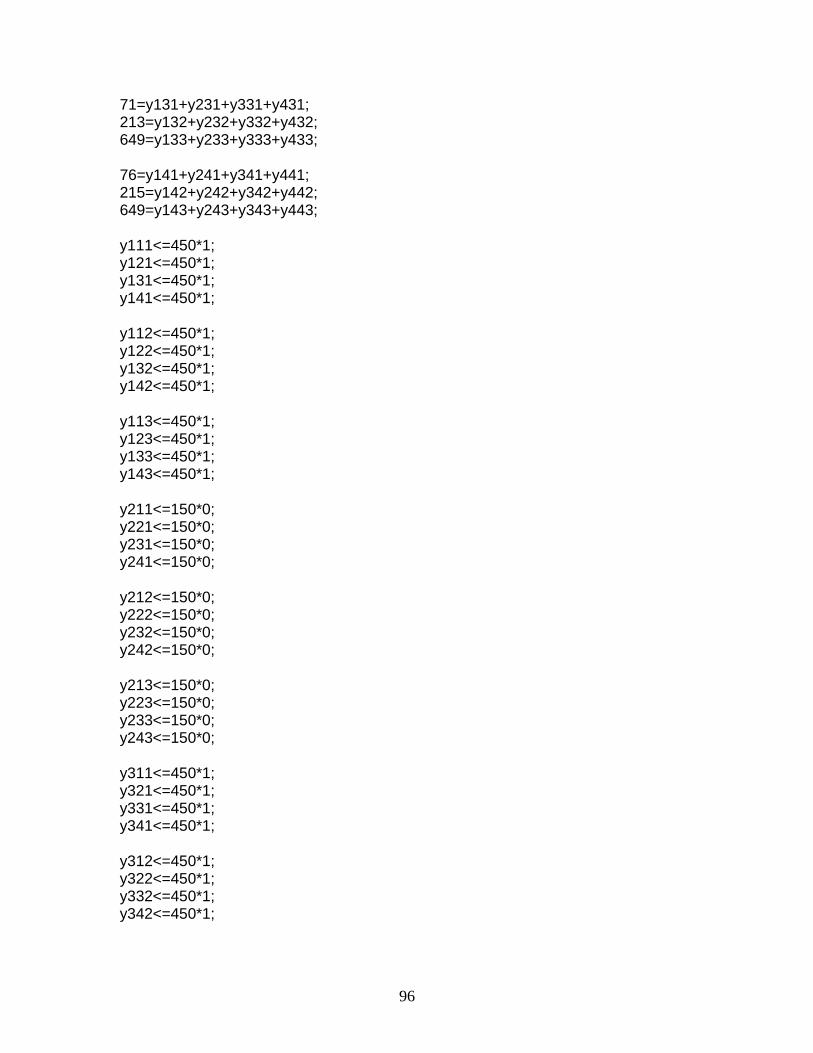
96
71=y131+y231+y331+y431; 213=y132+y232+y332+y432; 649=y133+y233+y333+y433; 76=y141+y241+y341+y441; 215=y142+y242+y342+y442; 649=y143+y243+y343+y443; y111<=450*1; y121<=450*1; y131<=450*1; y141<=450*1; y112<=450*1; y122<=450*1; y132<=450*1; y142<=450*1; y113<=450*1; y123<=450*1; y133<=450*1; y143<=450*1; y211<=150*0; y221<=150*0; y231<=150*0; y241<=150*0; y212<=150*0; y222<=150*0; y232<=150*0; y242<=150*0; y213<=150*0; y223<=150*0; y233<=150*0; y243<=150*0; y311<=450*1; y321<=450*1; y331<=450*1; y341<=450*1; y312<=450*1; y322<=450*1; y332<=450*1; y342<=450*1;
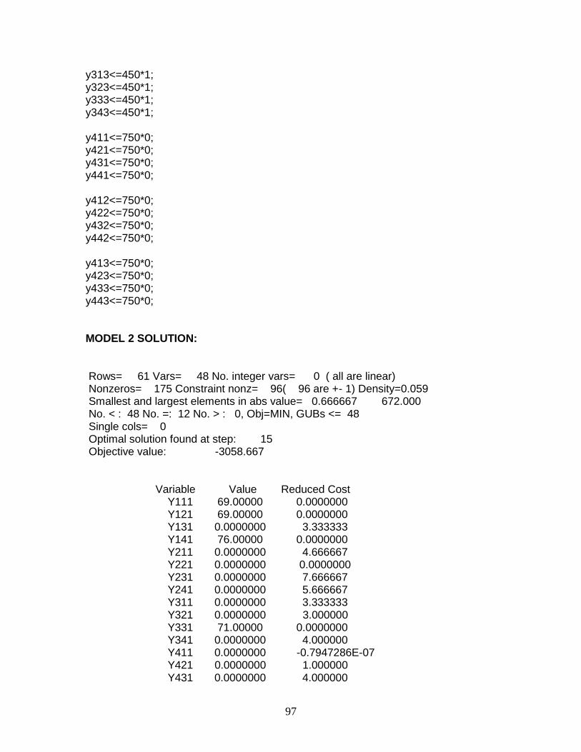
97
y313<=450*1; y323<=450*1; y333<=450*1; y343<=450*1; y411<=750*0; y421<=750*0; y431<=750*0; y441<=750*0; y412<=750*0; y422<=750*0; y432<=750*0; y442<=750*0; y413<=750*0; y423<=750*0; y433<=750*0; y443<=750*0; MODEL 2 SOLUTION: Rows= 61 Vars= 48 No. integer vars= 0 ( all are linear) Nonzeros= 175 Constraint nonz= 96( 96 are +- 1) Density=0.059 Smallest and largest elements in abs value= 0.666667 672.000 No. < : 48 No. =: 12 No. > : 0, Obj=MIN, GUBs <= 48 Single cols= 0 Optimal solution found at step: 15 Objective value: -3058.667 Variable Value Reduced Cost Y111 69.00000 0.0000000 Y121 69.00000 0.0000000 Y131 0.0000000 3.333333 Y141 76.00000 0.0000000 Y211 0.0000000 4.666667 Y221 0.0000000 0.0000000 Y231 0.0000000 7.666667 Y241 0.0000000 5.666667 Y311 0.0000000 3.333333 Y321 0.0000000 3.000000 Y331 71.00000 0.0000000 Y341 0.0000000 4.000000 Y411 0.0000000 -0.7947286E-07 Y421 0.0000000 1.000000 Y431 0.0000000 4.000000
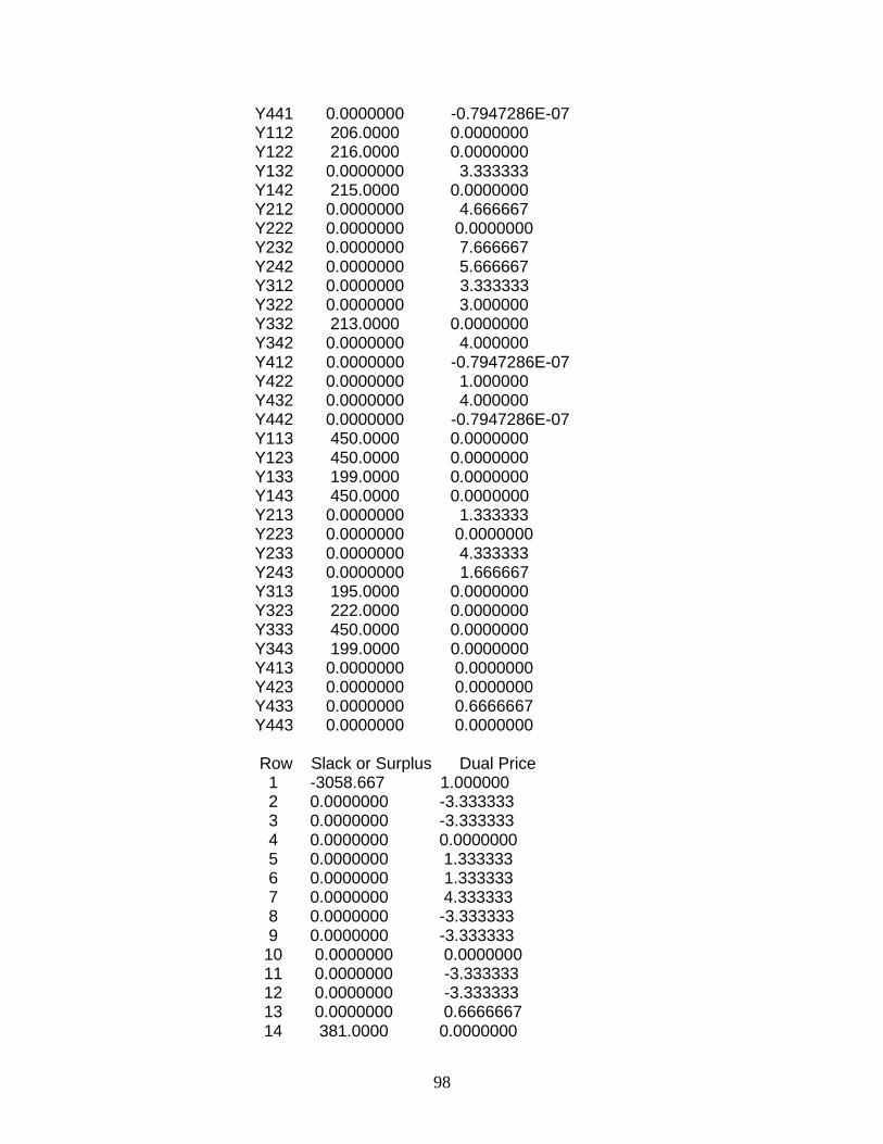
98
Y441 0.0000000 -0.7947286E-07 Y112 206.0000 0.0000000 Y122 216.0000 0.0000000 Y132 0.0000000 3.333333 Y142 215.0000 0.0000000 Y212 0.0000000 4.666667 Y222 0.0000000 0.0000000 Y232 0.0000000 7.666667 Y242 0.0000000 5.666667 Y312 0.0000000 3.333333 Y322 0.0000000 3.000000 Y332 213.0000 0.0000000 Y342 0.0000000 4.000000 Y412 0.0000000 -0.7947286E-07 Y422 0.0000000 1.000000 Y432 0.0000000 4.000000 Y442 0.0000000 -0.7947286E-07 Y113 450.0000 0.0000000 Y123 450.0000 0.0000000 Y133 199.0000 0.0000000 Y143 450.0000 0.0000000 Y213 0.0000000 1.333333 Y223 0.0000000 0.0000000 Y233 0.0000000 4.333333 Y243 0.0000000 1.666667 Y313 195.0000 0.0000000 Y323 222.0000 0.0000000 Y333 450.0000 0.0000000 Y343 199.0000 0.0000000 Y413 0.0000000 0.0000000 Y423 0.0000000 0.0000000 Y433 0.0000000 0.6666667 Y443 0.0000000 0.0000000 Row Slack or Surplus Dual Price 1 -3058.667 1.000000 2 0.0000000 -3.333333 3 0.0000000 -3.333333 4 0.0000000 0.0000000 5 0.0000000 1.333333 6 0.0000000 1.333333 7 0.0000000 4.333333 8 0.0000000 -3.333333 9 0.0000000 -3.333333 10 0.0000000 0.0000000 11 0.0000000 -3.333333 12 0.0000000 -3.333333 13 0.0000000 0.6666667 14 381.0000 0.0000000
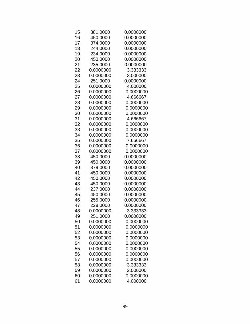
99
15 381.0000 0.0000000 16 450.0000 0.0000000 17 374.0000 0.0000000 18 244.0000 0.0000000 19 234.0000 0.0000000 20 450.0000 0.0000000 21 235.0000 0.0000000 22 0.0000000 3.333333 23 0.0000000 3.000000 24 251.0000 0.0000000 25 0.0000000 4.000000 26 0.0000000 0.0000000 27 0.0000000 4.666667 28 0.0000000 0.0000000 29 0.0000000 0.0000000 30 0.0000000 0.0000000 31 0.0000000 4.666667 32 0.0000000 0.0000000 33 0.0000000 0.0000000 34 0.0000000 0.0000000 35 0.0000000 7.666667 36 0.0000000 0.0000000 37 0.0000000 0.0000000 38 450.0000 0.0000000 39 450.0000 0.0000000 40 379.0000 0.0000000 41 450.0000 0.0000000 42 450.0000 0.0000000 43 450.0000 0.0000000 44 237.0000 0.0000000 45 450.0000 0.0000000 46 255.0000 0.0000000 47 228.0000 0.0000000 48 0.0000000 3.333333 49 251.0000 0.0000000 50 0.0000000 0.0000000 51 0.0000000 0.0000000 52 0.0000000 0.0000000 53 0.0000000 0.0000000 54 0.0000000 0.0000000 55 0.0000000 0.0000000 56 0.0000000 0.0000000 57 0.0000000 0.0000000 58 0.0000000 3.333333 59 0.0000000 2.000000 60 0.0000000 0.0000000 61 0.0000000 4.000000
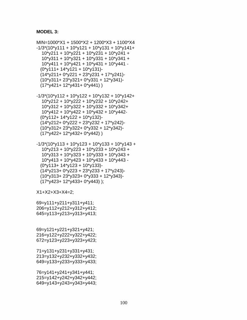
100
MODEL 3: MIN=1000*X1 + 1500*X2 + 1200*X3 + 1100*X4 -1/3*(10*y111 + 10*y121 + 10*y131 + 10*y141+ 10*y211 + 10*y221 + 10*y231 + 10*y241 + 10*y311 + 10*y321 + 10*y331 + 10*y341 + 10*y411 + 10*y421 + 10*y431 + 10*y441 - (0*y111+ 14*y121 + 10*y131)- (14*y211+ 0*y221 + 23*y231 + 17*y241)- (10*y311+ 23*y321+ 0*y331 + 12*y341)- (17*y421+ 12*y431+ 0*y441) ) -1/3*(10*y112 + 10*y122 + 10*y132 + 10*y142+ 10*y212 + 10*y222 + 10*y232 + 10*y242+ 10*y312 + 10*y322 + 10*y332 + 10*y342+ 10*y412 + 10*y422 + 10*y432 + 10*y442- (0*y112+ 14*y122 + 10*y132)- (14*y212+ 0*y222 + 23*y232 + 17*y242)- (10*y312+ 23*y322+ 0*y332 + 12*y342)- (17*y422+ 12*y432+ 0*y442) ) -1/3*(10*y113 + 10*y123 + 10*y133 + 10*y143 + 10*y213 + 10*y223 + 10*y233 + 10*y243 + 10*y313 + 10*y323 + 10*y333 + 10*y343 + 10*y413 + 10*y423 + 10*y433 + 10*y443 - (0*y113+ 14*y123 + 10*y133)- (14*y213+ 0*y223 + 23*y233 + 17*y243)- (10*y313+ 23*y323+ 0*y333 + 12*y343)- (17*y423+ 12*y433+ 0*y443) ); X1+X2+X3+X4=2; 69=y111+y211+y311+y411; 206=y112+y212+y312+y412; 645=y113+y213+y313+y413; 69=y121+y221+y321+y421; 216=y122+y222+y322+y422; 672=y123+y223+y323+y423; 71=y131+y231+y331+y431; 213=y132+y232+y332+y432; 649=y133+y233+y333+y433; 76=y141+y241+y341+y441; 215=y142+y242+y342+y442; 649=y143+y243+y343+y443;
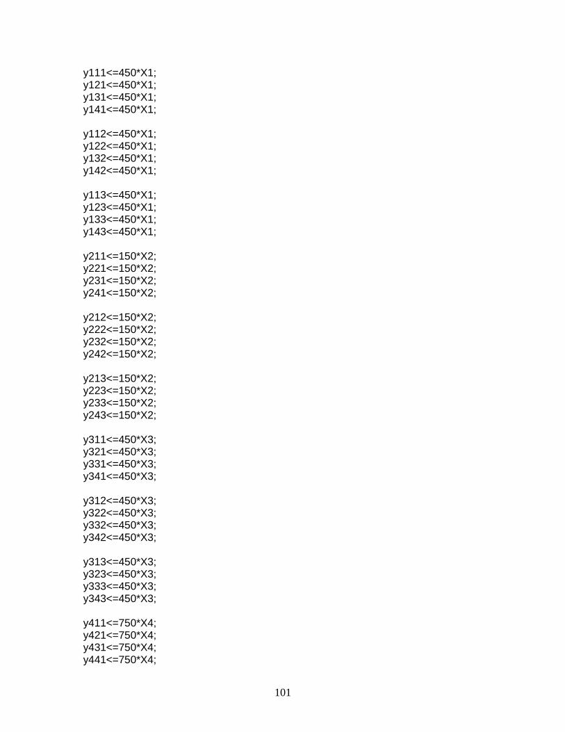
101
y111<=450*X1; y121<=450*X1; y131<=450*X1; y141<=450*X1; y112<=450*X1; y122<=450*X1; y132<=450*X1; y142<=450*X1; y113<=450*X1; y123<=450*X1; y133<=450*X1; y143<=450*X1; y211<=150*X2; y221<=150*X2; y231<=150*X2; y241<=150*X2; y212<=150*X2; y222<=150*X2; y232<=150*X2; y242<=150*X2; y213<=150*X2; y223<=150*X2; y233<=150*X2; y243<=150*X2; y311<=450*X3; y321<=450*X3; y331<=450*X3; y341<=450*X3; y312<=450*X3; y322<=450*X3; y332<=450*X3; y342<=450*X3; y313<=450*X3; y323<=450*X3; y333<=450*X3; y343<=450*X3; y411<=750*X4; y421<=750*X4; y431<=750*X4; y441<=750*X4;
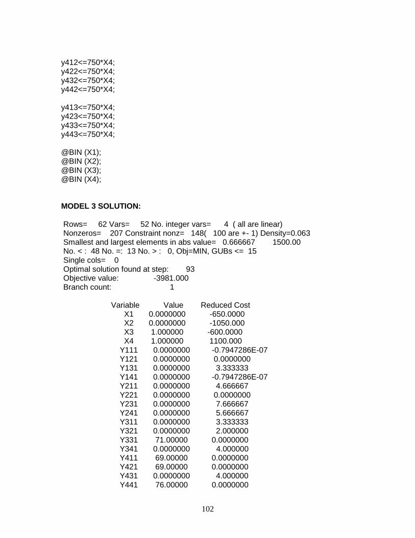
102
y412<=750*X4; y422<=750*X4; y432<=750*X4; y442<=750*X4; y413<=750*X4; y423<=750*X4; y433<=750*X4; y443<=750*X4; @BIN (X1); @BIN (X2); @BIN (X3); @BIN (X4); MODEL 3 SOLUTION: Rows= 62 Vars= 52 No. integer vars= 4 ( all are linear) Nonzeros= 207 Constraint nonz= 148( 100 are +- 1) Density=0.063 Smallest and largest elements in abs value= 0.666667 1500.00 No. < : 48 No. =: 13 No. > : 0, Obj=MIN, GUBs <= 15 Single cols= 0 Optimal solution found at step: 93 Objective value: -3981.000 Branch count: 1 Variable Value Reduced Cost X1 0.0000000 -650.0000 X2 0.0000000 -1050.000 X3 1.000000 -600.0000 X4 1.000000 1100.000 Y111 0.0000000 -0.7947286E-07 Y121 0.0000000 0.0000000 Y131 0.0000000 3.333333 Y141 0.0000000 -0.7947286E-07 Y211 0.0000000 4.666667 Y221 0.0000000 0.0000000 Y231 0.0000000 7.666667 Y241 0.0000000 5.666667 Y311 0.0000000 3.333333 Y321 0.0000000 2.000000 Y331 71.00000 0.0000000 Y341 0.0000000 4.000000 Y411 69.00000 0.0000000 Y421 69.00000 0.0000000 Y431 0.0000000 4.000000 Y441 76.00000 0.0000000
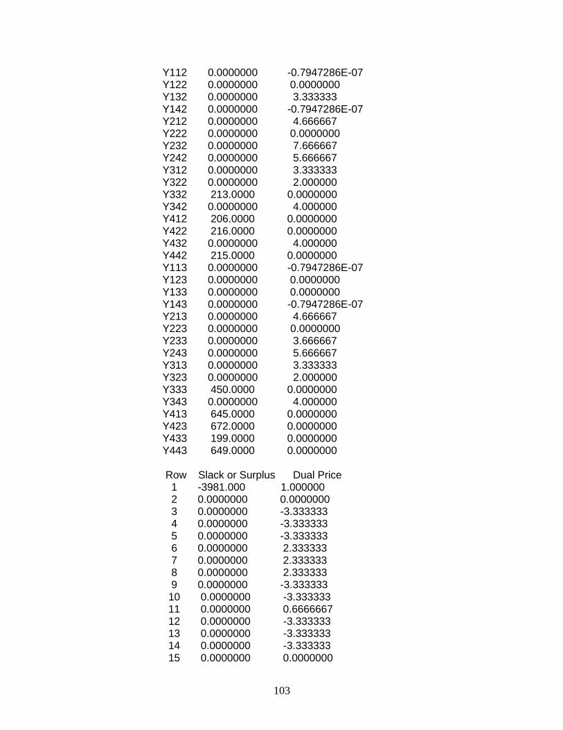
103
Y112 0.0000000 -0.7947286E-07 Y122 0.0000000 0.0000000 Y132 0.0000000 3.333333 Y142 0.0000000 -0.7947286E-07 Y212 0.0000000 4.666667 Y222 0.0000000 0.0000000 Y232 0.0000000 7.666667 Y242 0.0000000 5.666667 Y312 0.0000000 3.333333 Y322 0.0000000 2.000000 Y332 213.0000 0.0000000 Y342 0.0000000 4.000000 Y412 206.0000 0.0000000 Y422 216.0000 0.0000000 Y432 0.0000000 4.000000 Y442 215.0000 0.0000000 Y113 0.0000000 -0.7947286E-07 Y123 0.0000000 0.0000000 Y133 0.0000000 0.0000000 Y143 0.0000000 -0.7947286E-07 Y213 0.0000000 4.666667 Y223 0.0000000 0.0000000 Y233 0.0000000 3.666667 Y243 0.0000000 5.666667 Y313 0.0000000 3.333333 Y323 0.0000000 2.000000 Y333 450.0000 0.0000000 Y343 0.0000000 4.000000 Y413 645.0000 0.0000000 Y423 672.0000 0.0000000 Y433 199.0000 0.0000000 Y443 649.0000 0.0000000 Row Slack or Surplus Dual Price 1 -3981.000 1.000000 2 0.0000000 0.0000000 3 0.0000000 -3.333333 4 0.0000000 -3.333333 5 0.0000000 -3.333333 6 0.0000000 2.333333 7 0.0000000 2.333333 8 0.0000000 2.333333 9 0.0000000 -3.333333 10 0.0000000 -3.333333 11 0.0000000 0.6666667 12 0.0000000 -3.333333 13 0.0000000 -3.333333 14 0.0000000 -3.333333 15 0.0000000 0.0000000

104
16 0.0000000 1.000000 17 0.0000000 0.0000000 18 0.0000000 0.0000000 19 0.0000000 0.0000000 20 0.0000000 1.000000 21 0.0000000 0.0000000 22 0.0000000 0.0000000 23 0.0000000 0.0000000 24 0.0000000 1.000000 25 0.0000000 0.6666667 26 0.0000000 0.0000000 27 0.0000000 0.0000000 28 0.0000000 5.666667 29 0.0000000 0.0000000 30 0.0000000 0.0000000 31 0.0000000 0.0000000 32 0.0000000 5.666667 33 0.0000000 0.0000000 34 0.0000000 0.0000000 35 0.0000000 0.0000000 36 0.0000000 5.666667 37 0.0000000 0.0000000 38 0.0000000 0.0000000 39 450.0000 0.0000000 40 450.0000 0.0000000 41 379.0000 0.0000000 42 450.0000 0.0000000 43 450.0000 0.0000000 44 450.0000 0.0000000 45 237.0000 0.0000000 46 450.0000 0.0000000 47 450.0000 0.0000000 48 450.0000 0.0000000 49 0.0000000 4.000000 50 450.0000 0.0000000 51 681.0000 0.0000000 52 681.0000 0.0000000 53 750.0000 0.0000000 54 674.0000 0.0000000 55 544.0000 0.0000000 56 534.0000 0.0000000 57 750.0000 0.0000000 58 535.0000 0.0000000 59 105.0000 0.0000000 60 78.00000 0.0000000 61 551.0000 0.0000000 62 101.0000 0.0000000

105
APPENDIX J – RESPONSIBILITIES OF GROUP MEMBERS INTRODUCTION - Javaneh Zavari PROBLEM - Jenny Leung OBJECTIVE - Jenny Leung LITERATURE REVIEW - Javaneh Zavari & Jenny Leung SUPPLY CHAIN DESIGN FOR DISTRIBUTION CENTRES - Javaneh Zavari & Jenny Leung APPLICATION OF MODEL - Javaneh Zavari & Jenny Leung RESULTS - Javaneh Zavari & Jenny Leung CONCLUSION - Javaneh Zavari & Jenny Leung REFERENCES - Javaneh Zavari & Jenny Leung APPENDICES - Javaneh Zavari & Jenny Leung