support motion effects in a timber trestle bridge ... · pdf filethe axisvm model was...

Support Motion Effects in a Timber Trestle Bridge: Physical and Analytical Modeling

Steven A. Babcock, M.S. Richard M. Gutkowski, Ph.D., P.E.

Wayne A. Charlie, Ph.D., P.E. Jeno Balogh, Ph.D.

October 2006

ii

Acknowledgments This report was prepared with funds provided by the U.S. Department of Transportation to the Mountain Plains Consortium. MPC universities include North Dakota State University, Colorado State University (CSU), University of Wyoming, and University of Utah. The authors appreciate the assistance of Misty Butler, Travis Burgers, and Kathryn Sednick, who all assisted in conducting the research and testing.

Disclaimer The contents of this report reflect the views of the authors, who are responsible for the facts and the accuracy of the information presented. This document is disseminated under the sponsorship of the Department of Transportation, University Transportation Centers Program, in the interest of information exchange. The U.S. Government assumes no liability for the contents or use thereof.

iii

Abstract A representative one-tenth scale model of an open-deck three-span timber trestle bridge was constructed and subjected to load testing in the laboratory. The scaled timber trestle bridge incorporated a realistic wooden pile foundation in sandy soil. A computer-based analytical model was created with AxisVM software. The analytical model was used to predict the behavior of the physical model. The three-span complete timber trestle bridge model was constructed out of common dimension Douglas Fir. Each span was 1176 mm (48 in) long and utilized two semi-continuous bridge chords. Peeled pine poles were used in the pile foundation. This foundation type was used to create support motions similar to those observed in previous field testing. Wood crossties were also included in the physical specimen. Observed support motions of the physical specimen were similar to motions observed in field bridge tests. The AxisVM model was successful in predicting the behavior of the physical specimen. Typically, predicted deflections were within 5% to 10% of the measured values. The support motion created by the pile-soil interaction was also modeled successfully by using a linear spring approximation.

iv

Table of Contents 1. Introduction ...................................................................................................................................1

1.1 Timber Bridges .......................................................................................................................1 1.2 Background.............................................................................................................................1 1.3 Description of an Open Deck Timber Trestle Bridge .............................................................1 1.4 Background to the Research ...................................................................................................3

2. Literature Review..........................................................................................................................4

2.1 Railroad Bridge Load Testing.................................................................................................4 2.2 Timber Trestle Railroad Bridge Load Testing ........................................................................4 2.3 Study of an Open-Deck Skewed Timber Trestle Railroad Bridge..........................................4 2.4 Testing and Analysis of Timber Trestle Railroad Bridge Chords...........................................5

3. Description of Physical Bridge Model .........................................................................................6

3.1 Bridge Model Design..............................................................................................................6 3.2 Scaling of Model Bridge Stringers........................................................................................11 3.3 Substructure Description.......................................................................................................13 3.4 Pile Spacing and Soil Container ...........................................................................................13 3.5 Pile Installation .....................................................................................................................15

4. Materials Testing.........................................................................................................................17

4.1 Discussion of Important Properties.......................................................................................17 4.2 Pile Materials Testing ...........................................................................................................17 4.3 Bridge Model Component MOE Testing..............................................................................19 4.4 Simply Supported Beam Test ...............................................................................................19 4.5 Cantilever Beam Test of Tie Rail Members .........................................................................23

5. Testing of Substructure Strength...............................................................................................25

5.1 Load Application System......................................................................................................25 5.2 Ultimate Capacity Testing of the Test Piles..........................................................................25 5.3 Results of the Pile Load Test ................................................................................................26 5.4 Stiffness Testing of the Pile Groups of the Specimen...........................................................27 5.5 Results of the Pile Group Load Tests....................................................................................28 5.6 Alternative Method to Calculate Substructure Stiffness.......................................................30

6. Testing of Bridge Model Specimen ............................................................................................32

6.1 Measurement Method ...........................................................................................................32 6.2 Leica NA2 Auto-Level and Leica GMP3 Optical Micrometer.............................................32 6.3 Measurement Devices...........................................................................................................32 6.4 Measurement Recording .......................................................................................................34 6.5 Load Application ..................................................................................................................35 6.6 Load Testing of the Specimen ..............................................................................................36

6.6.1 Load Test #1 ...................................................................................................................37 6.6.2 Load Tests #2 and #3......................................................................................................37 6.6.3 Load Test #4 ...................................................................................................................37

v

7. Description of Computer Based Bridge Model.........................................................................38 7.1 AxisVM ................................................................................................................................38 7.2 Description of Utilized Elements..........................................................................................38 7.3 Description of Bridge Model ................................................................................................41

8. Comparison of Load Testing Results to AxisVM Prediction...................................................47

8.1 Comparison Methods ............................................................................................................47 8.1 Comparison of AxisVM Model #2 to Load Test #2 .............................................................47 8.3 Comparison of AxisVM Model #3 to Load Test #3 .............................................................51 8.4 Comparison of AxisVM Model #4 to Load Test #4 .............................................................55

9. Observations and Conclusions ...................................................................................................60

9.1 Observations .........................................................................................................................60 9.2 Conclusions...........................................................................................................................60

References ....................................................................................................................................63 Appendices (See note below) Appendix A: Construction Drawing for the Physical Specimen Appendix B: Material Property Tests for all Bridge Components Appendix C: Pile Tests Appendix D: Plots of All Load Test Results Appendix E: Plots of AxisVM Predictions Appendix F: Plots Comparing Load Tests and AxisVM Predictions Appendix G: Measured Gaps between Stringers and Crossties Appendix H: Proving Ring Calibration Plot Appendix I: Soil Data for Sand Used Appendix J: Substructure Stiffness Calculation Example using Method 2 NOTE: Appendices available from: Mountain Plains Consortium - Colorado State University c/o Dr. Richard Gutkowski, Director Engineering Research Center Colorado State University Fort Collins, Colorado 80523

vi

List of Tables

Table 4.1 Young’s Modulus and Ultimate Strength Results from Compression Tests on Pile Material................................................................................................................19

Table 4.2 Flexural MOE and E Test Results for the 1219 mm (4 ft) Stringers ..........................21

Table 4.3 Flexural MOE and E Test Results for the 2438 mm (8 ft) Stringers ..........................21

Table 4.4 Flexural MOE and E Results for the 2273 mm (8 ft) Stringers ..................................22

Table 4.5 Flexural MOE and E Results for the 2997 mm (10 ft) Pile Cap Beam.......................23

Table 4.6 MOE Results from the Tie Rail Test ..........................................................................23

Table 8.1 ASSE Value for Load Test #2 ....................................................................................51



vii

List of Figures

Figure 1.1 General Configuration of an Open Deck Timber Trestle Bridges.............................2

Figure 1.2 Alternating Stringer Pattern of a Timber Trestle Bridge ...........................................2

Figure 3.1 Plan View of the Physical Bridge Model ..................................................................6

Figure 3.2 Isotropic Rendering of Bridge Model........................................................................7

Figure 3.3 Typical Pile Embedment into Sandy Soil ..................................................................8

Figure 3.4 Rigid Pile Connection to the Load Frame at the Abutments .....................................8

Figure 3.5 One Abutment of the Bridge Specimen.....................................................................9

Figure 3.6 Horizontal Stringer Bolts of One Bridge Chord ........................................................9

Figure 3.7 Attachment of Specimen Crossties..........................................................................10

Figure 3.8 Superstructure of the Bridge Model Specimen During Construction......................11

Figure 3.9 Completed Bridge Model Specimen........................................................................11

Figure 3.10 3-D Rendering of the Soil Container Used..............................................................13

Figure 3.11 3-D Rendering of the Vibration Device Used for Soil Compaction........................14

Figure 3.12 Selected Images of Soil Placement in the Container ...............................................15

Figure 3.13 Photograph and 3-D Rendering of the Pile Driver Apparatus .................................15

Figure 3.14 Selected Images of the Pile Driving Process ...........................................................16

Figure 4.1 General Configuration of the Simply Supported Beam Test Setup.........................19

Figure 4.2 Dimensions of the 1219 mm (4 ft) Stringer Flexural Test.......................................20

Figure 4.3 Dimensions of the 2438 mm (8 ft) Stringer Flexural Test.......................................21

Figure 4.4 Dimensions of the 2273 mm (8 ft) Crossties Flexural Test .....................................22

Figure 5.1 Proving Ring and Hydraulic Bottle Jack Used to Apply Loads ..............................25

Figure 5.2 Pile Group Load Test Setup and Test Equipment ...................................................26

viii

Figure 5.3 Plots of Pile Test Results of Pile C1........................................................................27

Figure 6.1 Leica NA2 Auto Level and Leice GMP3 Optical Micrometer................................32

Figure 6.2 'Scale Tree' and Enlarged Single Scale....................................................................33

Figure 6.3 Measurement Positions Along the Length of the physical Bridge Model ...............33

Figure 6.4 Plan View of the 3 Auto-Level Locations Used ......................................................34

Figure 6.5 3D Rendering and Photo of the Specimen Load Test Setup....................................35

Figure 6.6 Diagram of the Load Distribution to the Crossties ..................................................35

Figure 6.7 Load Location #1, Used in Load Tests #1 and #2 ...................................................36

Figure 6.8 Load Location #2, Used in Load Test #3 ................................................................36

Figure 6.9 Load Location #3, Used in Load Test #4 ................................................................42

Figure 7.1 Conceptual Image of a Beam Element and the Possible DOF’s..............................38

Figure 7.2 Conceptual Image of a Nodal Support Element and the Possible DOF’s ...............39

Figure 7.3 Conceptual Image of a Spring Element and the Possible DOF’s ............................39

Figure 7.4 Gap Element Active in Compression with Associated Force-Displacement Diagram................................................................................................................40

Figure 7.5 Conceptual Image of a Link Element and the Possible DOF’s ...............................40

Figure 7.6 Physical Bridge Specimen .......................................................................................41

Figure 7.7 AxisVM Model of the Physical Bridge Specimen ..................................................42

Figure 7.8 Pile Cap from Physical Specimen............................................................................42

Figure 7.9 Typical Pile Cap Modeled in AxisVM ....................................................................43

Figure 7.10 Bridge Superstructure of the Physical Specimen.....................................................44

Figure 7.11 Bridge Superstructure Model in AxisVM................................................................44

Figure 7.12 Application of the Load to the Physical Specimen..................................................46

Figure 7.13 Typical Application of Point Loads into the AxisVM Model .................................46

ix

Figure 8.1 Measurement Positions and Load Application for Load Test #2 and AxisVM Model #2 ...............................................................................................48

Figure 8.2 Deformed Shape of the Pile Caps Under 13344 N (3000 lb) of Load Test #2 ........48

Figure 8.3 Deflected Shape of Stringer 5 Under 13344 N of Load Test #2..............................49




Figure 8.7 Measurement Positions and Load Application for Load Test #3 and Axis VM Model #3........................................................................................51

Figure 8.8 Deformed Shape of the Pile Caps Under 13344 N of Load Test #3........................52





Figure 8.13 Measurement Positions and Load Application for Load Test #4 and Axis VM Model #4........................................................................................55

Figure 8.14 Deformed Shape of the Pile Caps Under 6672 N of Load Test #4..........................56

Figure 8.15 Deflected Shape of Stringer 5 Under 6672 N of Load Test #4................................57




1

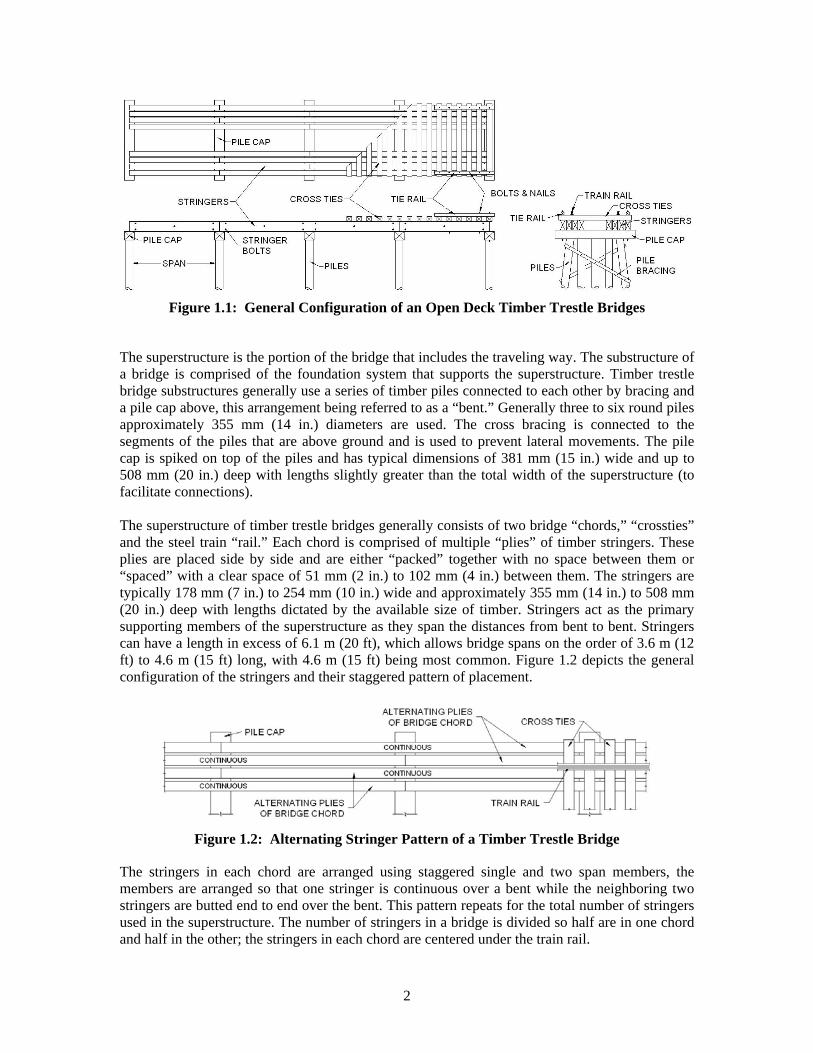
1. Introduction 1.1 Timber Bridges Timber was widely used as the primary construction material of bridges through most of history due to its availability and ease of use in construction. Only recently have wood’s structural qualities been evaluated [Troitsky, 1994]. More than one third of the United States is considered forestland, which is capable of producing large amounts of structural timber each year [Smith, 1999]. The availability of timber made it the most logical option for construction during the industrial revolution and western expansion of the United States well into the middle of the twentieth century. There are more than 71,000 highway and non-highway timber bridges in the United States [Ritter, 1990]. There are more than 2,900 km (1,800 miles) of timber railroad bridges in the United States [Ritter, 1992] and many of the timber railroad bridges have a trestle configuration. 1.2 Background Timber trestle bridges consist of longitudinal stringers supported by intermittent bents that are typically supported by piles. The bridge deck is attached to the stringers. The stringers are the primary supporting structure of trestle bridges and are designed as simple span beams under the recommended loading [AITC, 1994]. Many timber trestle railroad bridges have been in services for more than 50 years. Some have been performing successfully for nearly 100 years [Byers, 1996]. During such long operating lives these bridges have endured material deterioration and increases in the train loads. The ability of these bridges to perform successfully under such conditions stems, in part, from the conservative nature by which the bridges were designed. In addition, the wood used in newer timber trestle bridges is typically chemically treated with creosote. This treatment helps reduce the rate of wood weathering and decay. Increased loads are a basis for ongoing consideration of a major increase in the minimum design load requirement. Consequently, in the early 1990’s, the Association of American Railroads (AAR) initiated an extensive program to evaluate the strength of existing bridges, whether comprised of timber or of other construction materials. Also the AAR has been pursuing methods to rehabilitate in-situ bridges to increase bridge strength and stiffness up to the impending standards. One approach to rehabilitate the timber trestle bridges is to add additional members and/or replace deteriorated ones. Addition of intermediate supports to bridges has also been considered. 1.3 Description of an Open Deck Timber Trestle Bridge The design of timber trestle bridges is specified and controlled by the American Railway Engineering and Maintenance Association (AREMA) via its design manual [AREMA, 1995]. This manual also specifies the construction, maintenance and inspection procedures for timber railroad bridges. Figure 1.1 below illustrates the general configuration of a standard “open deck timber trestle railroad bridge.” This bridge is composed of two distinct sections, that of a “superstructure” and a “substructure.”

2

Figure 1.1: General Configuration of an Open Deck Timber Trestle Bridges

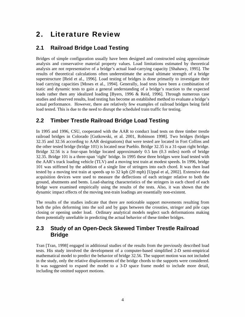
The superstructure is the portion of the bridge that includes the traveling way. The substructure of a bridge is comprised of the foundation system that supports the superstructure. Timber trestle bridge substructures generally use a series of timber piles connected to each other by bracing and a pile cap above, this arrangement being referred to as a “bent.” Generally three to six round piles approximately 355 mm (14 in.) diameters are used. The cross bracing is connected to the segments of the piles that are above ground and is used to prevent lateral movements. The pile cap is spiked on top of the piles and has typical dimensions of 381 mm (15 in.) wide and up to 508 mm (20 in.) deep with lengths slightly greater than the total width of the superstructure (to facilitate connections). The superstructure of timber trestle bridges generally consists of two bridge “chords,” “crossties” and the steel train “rail.” Each chord is comprised of multiple “plies” of timber stringers. These plies are placed side by side and are either “packed” together with no space between them or “spaced” with a clear space of 51 mm (2 in.) to 102 mm (4 in.) between them. The stringers are typically 178 mm (7 in.) to 254 mm (10 in.) wide and approximately 355 mm (14 in.) to 508 mm (20 in.) deep with lengths dictated by the available size of timber. Stringers act as the primary supporting members of the superstructure as they span the distances from bent to bent. Stringers can have a length in excess of 6.1 m (20 ft), which allows bridge spans on the order of 3.6 m (12 ft) to 4.6 m (15 ft) long, with 4.6 m (15 ft) being most common. Figure 1.2 depicts the general configuration of the stringers and their staggered pattern of placement.

Figure 1.2: Alternating Stringer Pattern of a Timber Trestle Bridge

The stringers in each chord are arranged using staggered single and two span members, the members are arranged so that one stringer is continuous over a bent while the neighboring two stringers are butted end to end over the bent. This pattern repeats for the total number of stringers used in the superstructure. The number of stringers in a bridge is divided so half are in one chord and half in the other; the stringers in each chord are centered under the train rail.

3

Transverse wood crossties are attached above the stringers and typically have a 203 mm (8 in.) square cross-section. The crossties act to distribute the loads applied to the rail down to the stringers. The AREMA manual specifies that the spacing between the crossties cannot exceed 203 mm (8 in.) [AREMA, 1995]. This spacing of crossties is the primary reason that a bridge is classified as an “open deck” bridge. If there is no space between the crossties the bridge is classified as a “closed deck” bridge. The rail rests upon rail platens that transfer the trainloads onto the crossties, then down to the stringers and finally to the foundation and ground below. Each length of rail is spiked to the cross ties and connected to each other by a series of bolts and connection plates. The crossties are connected to the stringers by a combination of long bolts and spikes. Generally every third crosstie is bolted to the outer most stringer of each chord, and the intermediate two crossties are spiked to a timber “tie rail” that lies above the crossties above each chord. The intermediate crossties are not physically connected to the underlying stringers. The stringers are bolted to each other by horizontal bolts near the ends of and at mid-span of each span. The stringers are bolted horizontally with spacers (approximately 51 mm (2 in.) wide) between them if the stringers are not “packed.” The outer most stringer is then bolted down through the pile cap, which connects the superstructure to the substructure. This connection configuration results in the majority of stringers lacking vertical connection devices to both the crossties and the pile caps. They are held in place by the horizontal stringer bolts and by friction from bearing between the crossties and pile caps. This configuration allows for irregular gaps to exist between the stringers, crossties and pile caps. 1.4 Background to the Research The AAR has a conducted cooperative research with several universities to investigate the condition of timber bridges in their inventory. Colorado State University (CSU) has been involved in this research since 1995. CSU’s involvement began with the field-testing of three timber trestle bridges in Colorado, [Uppal et al. 2002] under static and moving trainloads, as well as ramp loads. These tests investigated the load paths of each bridge. A subsequent laboratory study of a full-scale timber trestle railroad bridge chord was conducted at CSU to further investigate the load paths through the chord [Doyle et al., 2000]. Complications occurred due to the uplift of the ends of the chords of the multi-span specimens. Later, improved tests were conducted to eliminate the uplift. This report presents the results of the most recent phase of laboratory research. The effects of support movements observed in the field test were examined by physical laboratory testing and computer-based structural modeling using AxisVM software [Inter-CAD. Kft, 2004]. The goal of this research was to begin developing analytical tools to help predict the performance capabilities of in-situ bridges with support motions included.

4

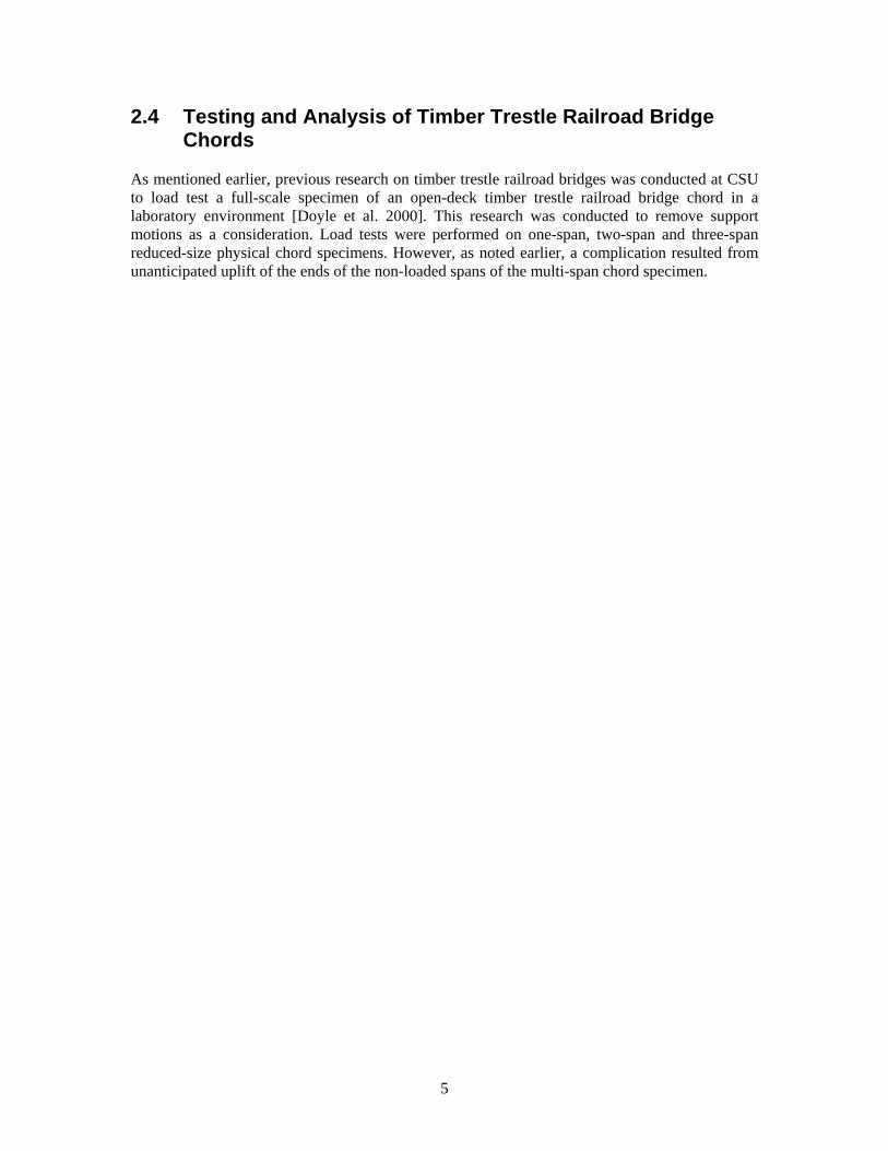
2. Literature Review 2.1 Railroad Bridge Load Testing Bridges of simple configuration usually have been designed and constructed using approximate analysis and conservative material property values. Load limitations estimated by theoretical analysis are not representative of a bridge’s actual load-carrying capacity [Shahawy, 1995]. The results of theoretical calculations often underestimate the actual ultimate strength of a bridge superstructure [Reid et al., 1996]. Load testing of bridges is done primarily to investigate their load carrying capacities [Moses et al., 1994]. Generally, load tests have been a combination of static and dynamic tests to gain a general understanding of a bridge’s reaction to the expected loads rather then any idealized loading [Byers, 1996 & Reid, 1996]. Through numerous case studies and observed results, load testing has become an established method to evaluate a bridge’s actual performance. However, there are relatively few examples of railroad bridges being field load tested. This is due to the need to disrupt the scheduled train traffic for testing. 2.2 Timber Trestle Railroad Bridge Load Testing In 1995 and 1996, CSU, cooperated with the AAR to conduct load tests on three timber trestle railroad bridges in Colorado [Gutkowski, et al. 2001, Robinson 1998]. Two bridges (bridges 32.35 and 32.56 according to AAR designations) that were tested are located in Fort Collins and the other tested bridge (bridge 101) is located near Pueblo. Bridge 32.35 is a 31-span right bridge. Bridge 32.56 is a four-span bridge located approximately 0.5 km (0.3 miles) north of bridge 32.35. Bridge 101 is a three-span ‘right’ bridge. In 1995 these three bridges were load tested with the AAR’s track loading vehicle (TLV) and a moving test train at modest speeds. In 1996, bridge 101 was stiffened by the addition of a single line of stringers into each chord. It was then load tested by a moving test train at speeds up to 32 kph (20 mph) [Uppal et al, 2002]. Extensive data acquisition devices were used to measure the deflections of each stringer relative to both the ground, abutments and bents. Load-sharing characteristics of the stringers in each chord of each bridge were examined empirically using the results of the tests. Also, it was shown that the dynamic impact effects of the moving test-train loadings are essentially non-existent. The results of the studies indicate that there are noticeable support movements resulting from both the piles deforming into the soil and by gaps between the crossties, stringer and pile caps closing or opening under load. Ordinary analytical models neglect such deformations making them potentially unreliable in predicting the actual behavior of these timber bridges. 2.3 Study of an Open-Deck Skewed Timber Trestle Railroad

Bridge Tran [Tran, 1998] engaged in additional studies of the results from the previously described load tests. His study involved the development of a computer-based simplified 2-D semi-empirical mathematical model to predict the behavior of bridge 32.56. The support motion was not included in the study, only the relative displacements of the bridge chords to the supports were considered. It was suggested to expand the model to a 3-D space frame model to include more detail, including the omitted support motions.

5

2.4 Testing and Analysis of Timber Trestle Railroad Bridge Chords

As mentioned earlier, previous research on timber trestle railroad bridges was conducted at CSU to load test a full-scale specimen of an open-deck timber trestle railroad bridge chord in a laboratory environment [Doyle et al. 2000]. This research was conducted to remove support motions as a consideration. Load tests were performed on one-span, two-span and three-span reduced-size physical chord specimens. However, as noted earlier, a complication resulted from unanticipated uplift of the ends of the non-loaded spans of the multi-span chord specimen.

6

3. Description of Physical Bridge Model 3.1 Bridge Model Design A three-span bridge chord specimen with spans approximately 1.2 m (4 ft) long and a total length of 3.65 m (12 ft) was constructed. This physical model was positioned such that the spans were oriented from north to south in the laboratory because of the existing layout of the load frame used for the test set up. The layout of the specimen was controlled by a series of grid lines that allowed the bridge model to be oriented within the load frame. Figure 3.1 illustrates the plan view of the specimen in the steel load frame with the gridlines used. Three gridlines run south to north and are labeled with numbers increasing from west to east. Five gridlines run west to east and are labeled with letters increasing from south to north. The labels of the gridlines serve as the basis for the labeling of the components of the specimen. The intersections of the gridlines served to locate the position of the piles and were also used to label the piles. The remainder of the bridge orientation was controlled from the piles. Figure 3.1 illustrates the geometry of the specimen without the soil shown.

Figure 3.1: Plan View of the Physical Bridge Model

As shown in Figure 3.2 there were three piles per bent and abutment. The piles at each bent and abutment were laterally spaced at 229 mm (9 in.) center to center, with 1118 mm (44 in.) center to center between each bent and abutment. Also, three piles were located below the bridge, centered under the middle span. These three piles are designated as “test piles” and were load tested before constructing the bridge model to assess the ultimate load carrying capacity of each pile. All of the piles were constructed from peeled pine poles with approximate diameters of 64 mm (2.5 in.) The diameter of each pile varies along its length similar to actual timber piles. The larger ends of the piles had approximately a 66 mm (2.6 in.) diameter and the smaller end diameters were approximately 61 mm (2.4 in.) As illustrated in Figure 3.5, the piles at the abutments were rigidly connected to the steel load frame to prevent the uplift of the specimen ends These end piles were 375 mm (14.75 in.) long.

7

Figure 3.2: Isotropic Rendering of Bridge Model

Figure 3.4 shows an abutment of the bridge specimen. The abutment piles are clamped to a steel plate with steel “pile collars” and the plate was clamped to the steel load frame using ‘C’ clamps. The steel collars were tightened around the piles then steel screws were used to reinforce the collar’s connection to the pile. As shown in Figure 3.3 the interior bent piles and the test piles were 1016 mm (40 in.) long and were driven 940 mm (37 in.) into the soil, leaving a 279 mm (11 in.) space between the pile tips and the concrete floor of the laboratory. 89 mm (3.5 in.) square pile caps were attached to each set of piles with a single vertical steel nail into each pile. The pile caps were 610 mm (24 in.) long. Above the pile caps were two bridge chords. Each chord had a four ply, semi-continuous set of staggered stringer members typical of trestle bridges. The stringers were labeled according the pile caps they span and numbered from west to east. The stringer label “ST 1AB” indicates the west-most stringer spanning pile caps A and B, thus it is also a single-span member. “ST 1BDE” indicates the west-most two-span stringer spanning pile caps B, D and E. The stringers were 19 mm (0.75 in.) wide and 76 mm (3 in.) deep and had lengths of either 1219 mm (48 in.) or 2438 mm (96 in.) due to the staggered configuration used. The stringers were horizontally bolted together using five 6 mm (1/4 in.) diameter steel bolts per span with 13 mm (0.5 in.) spacers between each stringer. The outside to outside width of the two chords was 584 mm (23 in.) Figure 3.6 illustrates the horizontal stringer bolts used.

8

Figure 3.3: Typical Pile Embedment into Sandy Soil

Figure 3.4: Rigid Pile Connection to the Load Frame at the Abutments

Pile ‘C’ Clamp

Pile Collar Steel Plate

Load Frame

9

Figure 3.5: One Abutment of the Bridge Specimen

Figure 3.6: Horizontal Stringer Bolts of One Bridge Chord

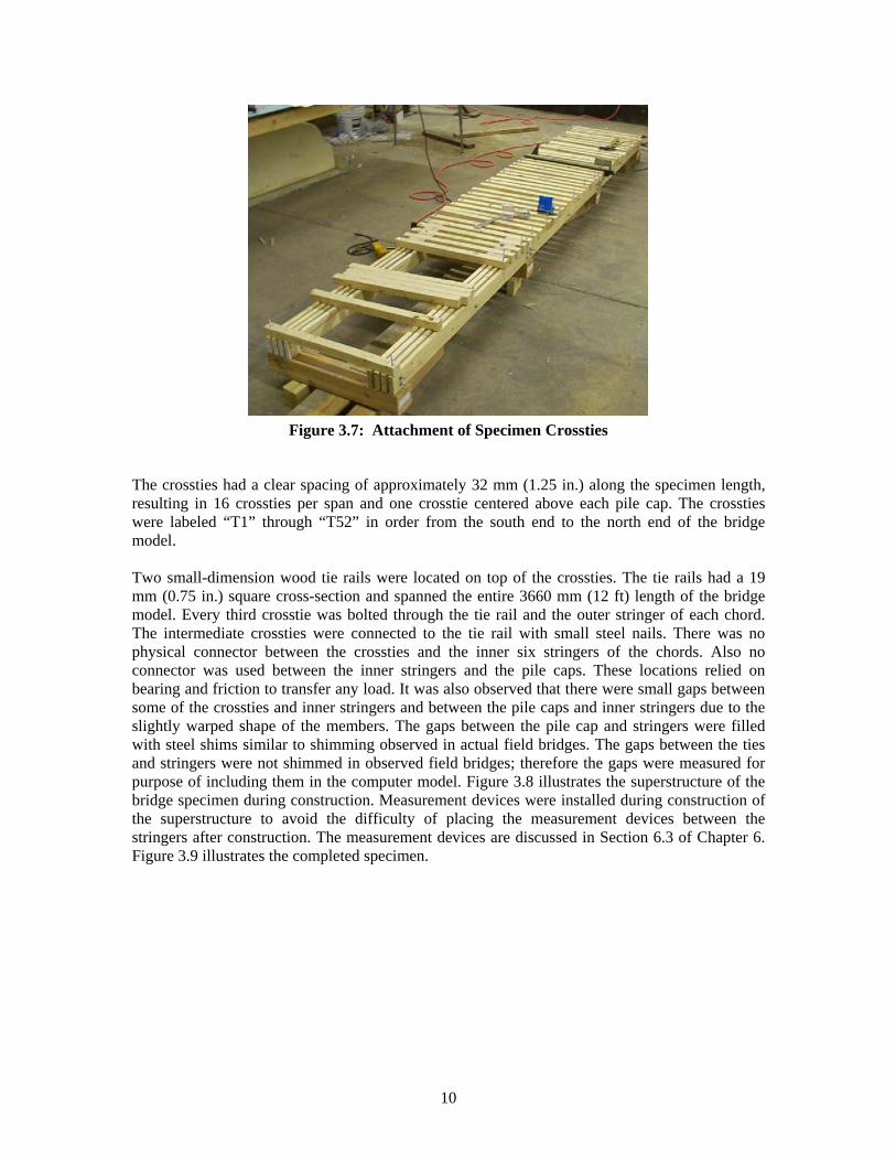
The chords were attached to the pile caps by 5 mm (3/8 in) diameter steel bolts that pass through the outermost stringer, the pile cap and one crosstie centered above the pile cap. Above the chords there were 52 crossties. Each crosstie had a 38 mm (1.5 in.) square cross-section and was 610 mm (24 in.) long. Figure 3.7 illustrates the connection of the crossties to the stringers.

10

Figure 3.7: Attachment of Specimen Crossties

The crossties had a clear spacing of approximately 32 mm (1.25 in.) along the specimen length, resulting in 16 crossties per span and one crosstie centered above each pile cap. The crossties were labeled “T1” through “T52” in order from the south end to the north end of the bridge model. Two small-dimension wood tie rails were located on top of the crossties. The tie rails had a 19 mm (0.75 in.) square cross-section and spanned the entire 3660 mm (12 ft) length of the bridge model. Every third crosstie was bolted through the tie rail and the outer stringer of each chord. The intermediate crossties were connected to the tie rail with small steel nails. There was no physical connector between the crossties and the inner six stringers of the chords. Also no connector was used between the inner stringers and the pile caps. These locations relied on bearing and friction to transfer any load. It was also observed that there were small gaps between some of the crossties and inner stringers and between the pile caps and inner stringers due to the slightly warped shape of the members. The gaps between the pile cap and stringers were filled with steel shims similar to shimming observed in actual field bridges. The gaps between the ties and stringers were not shimmed in observed field bridges; therefore the gaps were measured for purpose of including them in the computer model. Figure 3.8 illustrates the superstructure of the bridge specimen during construction. Measurement devices were installed during construction of the superstructure to avoid the difficulty of placing the measurement devices between the stringers after construction. The measurement devices are discussed in Section 6.3 of Chapter 6. Figure 3.9 illustrates the completed specimen.

11

Figure 3.8: Superstructure of the Bridge Model Specimen During Construction

Figure 3.9: Completed Bridge Model Specimen

3.2 Scaling of Model Bridge Stringers The dimensions of the stringers have a substantial effect on the behavior of the physical model. In addition, the stringers distribute the applied load to the piles and into the soil. Because the steel load frame supports the abutments and the interior bents are supported by a significantly less stiff soil, the stiffness of the stringers will have an effect on the load distribution into the abutments and bents. If the stringers are too stiff, the bridge will behave more like a single-span bridge with soft springs where the bents are rather than a three-span bridge. If the stringers were too flexible, their deflections for the estimated loading would too large and would deflect as if the pile cap supports were rigid and therefore measurable support motions would not be produced. It is important to scale the stiffness of the stringers so that measurable stringer deflections and support motions develop without initiating permanent pile deflection or high internal stresses in the specimen. The stringers for the bridge model specimen were scaled by stiffness to approximate those of bridge 101. The modulus of elasticity (MOE), cross-section dimension of

12

the field stringers and span lengths were known for this field bridge as well as load-deflection data. To scale the stiffness of the stringers of the specimen a stiffness parameter ‘Γ' was used. This parameter incorporated the MOE, moment of inertia (I) and span lengths (L) of the field bridge and the specimen, the actual values for these properties were 8.27 GPa (1,200 ksi), 1.1x109 mm4 (2730.67 in4) and 4369 mm (172 in.) respectively. Using this stiffness parameter and the ratio of load applied to the model and load applied to bridge 101 the stringer dimensions could be calculated.

LIMOE *

=Γ

⎟⎟⎠

⎞⎜⎜⎝

⎛⎟⎠⎞

⎜⎝⎛=⎟⎟

⎠

⎞⎜⎜⎝

⎛⎟⎠⎞

⎜⎝⎛⇒⎟⎟

⎠

⎞⎜⎜⎝

⎛Γ=⎟⎟

⎠

⎞⎜⎜⎝

⎛Γ

el

el

elbr

el

brel

elel

br

elbr P

PL

IMOEPP

LIMOE

PP

PP

mod

mod

mod101

mod

101mod

modmod

101

mod101

**

Using average values of MOE, moment of inertial (I) and span length (L) from the field test along with the expected MOE of 8.27 GPa (1.8E+6 psi) [AFPA, 2001] and design span length from the model specimen it was calculated.

⎟⎟⎠

⎞⎜⎜⎝

⎛⎟⎟⎠

⎞⎜⎜⎝

⎛⎟⎠⎞

⎜⎝⎛==

101

mod

mod

mod

101

3

mod*

12*

br

el

el

el

brel P

PMOE

LL

IMOEhbI

⎟⎟⎠

⎞⎜⎜⎝

⎛=⎟⎟

⎠

⎞⎜⎜⎝

⎛⎟⎠⎞

⎜⎝⎛

⎟⎟⎠

⎞⎜⎜⎝

⎛=

101

mod46

101

mod49

mod *105.196*4.12

1170*4369

101.1*27.8

br

el

br

elel P

Pmmx

PP

GPamm

mmmmxGPaI

To determine the load applied to the model the capacity of the pile foundation was used

( )( )( ) stringerN

stringerspilespileN

StringersPilestyPileCapaciP el /2168

86*/2891

##

mod ===

The load level applied to bridge 101 was 613 kN/stringer (138,000 lb/stringer).

12*10695

613168.2*105.196

34346

modhbmmx

KNKNmmxI el ==⎟

⎠⎞

⎜⎝⎛=

A stringer width of 19 mm (0.75 in.) was selected for the physical model because boards with that width are commonly available in many depths.

mmhhmmmmxI el 7612

*19106953

43mod =∴==

The cross-sectional dimensions of the scaled stringers were calculated to be 19 mm (0.75 in.) wide and 76 mm (3 in.) deep. The effects of pile cap size as well as the dimensions of crossties have not been studied before so no mathematical method of scaling their stiffness was used. It is assumed that the true structural effects of the crossties will be minimal because the applied test loads were centered above the bridge chords to simulate trainloads.

13

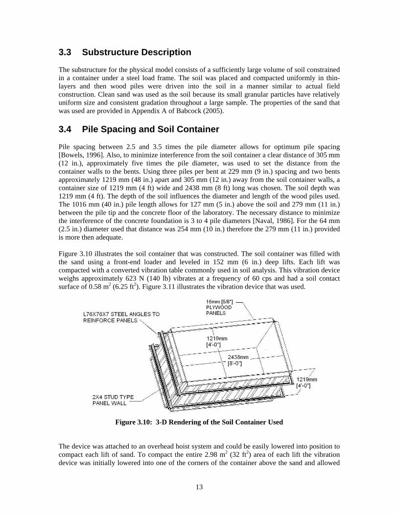
3.3 Substructure Description The substructure for the physical model consists of a sufficiently large volume of soil constrained in a container under a steel load frame. The soil was placed and compacted uniformly in thin-layers and then wood piles were driven into the soil in a manner similar to actual field construction. Clean sand was used as the soil because its small granular particles have relatively uniform size and consistent gradation throughout a large sample. The properties of the sand that was used are provided in Appendix A of Babcock (2005). 3.4 Pile Spacing and Soil Container Pile spacing between 2.5 and 3.5 times the pile diameter allows for optimum pile spacing [Bowels, 1996]. Also, to minimize interference from the soil container a clear distance of 305 mm (12 in.), approximately five times the pile diameter, was used to set the distance from the container walls to the bents. Using three piles per bent at 229 mm (9 in.) spacing and two bents approximately 1219 mm (48 in.) apart and 305 mm (12 in.) away from the soil container walls, a container size of 1219 mm (4 ft) wide and 2438 mm (8 ft) long was chosen. The soil depth was 1219 mm (4 ft). The depth of the soil influences the diameter and length of the wood piles used. The 1016 mm (40 in.) pile length allows for 127 mm (5 in.) above the soil and 279 mm (11 in.) between the pile tip and the concrete floor of the laboratory. The necessary distance to minimize the interference of the concrete foundation is 3 to 4 pile diameters [Naval, 1986]. For the 64 mm (2.5 in.) diameter used that distance was 254 mm (10 in.) therefore the 279 mm (11 in.) provided is more then adequate. Figure 3.10 illustrates the soil container that was constructed. The soil container was filled with the sand using a front-end loader and leveled in 152 mm (6 in.) deep lifts. Each lift was compacted with a converted vibration table commonly used in soil analysis. This vibration device weighs approximately 623 N (140 lb) vibrates at a frequency of 60 cps and had a soil contact surface of 0.58 m2 (6.25 ft2). Figure 3.11 illustrates the vibration device that was used.

Figure 3.10: 3-D Rendering of the Soil Container Used

The device was attached to an overhead hoist system and could be easily lowered into position to compact each lift of sand. To compact the entire 2.98 m2 (32 ft2) area of each lift the vibration device was initially lowered into one of the corners of the container above the sand and allowed

14

to vibrate unsupported for approximately thirty seconds. It was then moved to an adjacent location and allowed to vibrate for the same time period. This procedure continued until the entire lift was compacted. Then another lift of sand was placed and compacted using the same procedure. Figure 3.12 displays numerous images of the soil placing and compaction process. The soil container was filled completely using eight 152 mm (6 in.) lifts and the compaction process described. Once the soil was placed the gridlines were painted on to allow easy location of the piles. The soil was allowed to set in the container undisturbed for approximately one month to allow for any additional settlement of the material that could affect deflection and support motion measurements taken later

Figure 3.11: 3-D Rendering of the Vibration Device Used for Soil Compaction

15

Figure 3.12: Selected Images of Soil Placement in the Container

3.5 Pile Installation To follow field construction procedures the piles were driven into the sand foundation using a large vibrating mass located on the top of the wood piles. The pile driver was fabricated out of mild steel and had a final weight of approximately 2 kN (450 lb). Figure 3.13 illustrates the pile driving apparatus.

Figure 3.13: Photograph and 3-D Rendering of the Pile Driver Apparatus

16

The vibrating body of the table was retrofitted by attaching it to a vertically sliding plate that slid along vertical rails. The sliding plate has a steel collar in the center of the plate that centers the vibrating mass above the pile being driven. The vertical rails were attached to a rectangular base that was supported by steel beams that rested on the sides of the soil container, not on the sand. The rectangular base could be moved along the support beams allowing the setup to be used for all nine pile locations. The sliding plate contained mounts to enable one to bolt additional weight to the vibrating device, increasing the driving force that the system could generate. After each pile was cut to the specified length of 1016 mm (40 in.) they were driven into the sand. The pile driver was set up above the desired pile location and the vibrating mass and attached sliding plate was lifted up by an overhead hoist system, the pile was placed vertically under the mass, with the small diameter down. The mass was lowered to contact the pile, and then the vibrator was turned on and drove the pile into the sand. See Babcock (2005) for a plan view of the pile grid locations and relation to the bridge model and load frame as a whole. The pile at grid location D1 was driven first, then location C1 followed by B1, B3, C3, D3, D2, C2 and finally B2. This pattern was used to minimize setup alterations throughout the process. Researchers monitored the pile driving machinery and support setup at all times to insure proper pile installation. Figure 3.14 shows selected images of the pile-driving process.

Figure 3.14: Selected Images of the Pile-Driving Process

17

4. Materials Testing 4.1 Discussion of Important Properties To enable accurate computer modeling, specific material strength properties need to be determined for the individual components of the physical bridge model. The most relevant material property for the wood members is the modulus of elasticity (MOE). The MOE relates the linear deformation of wood to applied flexural loading. This property is specific to wood because of the very low shear stiffness that occurs in wood, roughly one-sixth of the axial stiffness [Criswell, 1982]. The low shearing modulus of wood can result in significant elastic deformation caused by shear stresses. In practical usage the MOE combines the deflection caused by flexural strains and the deflection caused by the shear deformation. Also it is important to evaluate the Young’s Modulus (E) of the wood piles used. E relates the axial strains of a member to applied axial stresses. The difference between E and the MOE is that the former does not include shear deformation and the latter does. The MOE value for each component was evaluated by conducting non-destructive beam tests. The stringers, pile caps, and cross ties were tested as simply supported beams, and the tie rails were tested as cantilever beams. The details of the beam tests are described in subsequent sections. Segments of the wood pile material were tested for their E values by conducting standard destructive compression tests. The specific procedure for the compression tests is discussed in the next section 4.2 Pile Materials Testing Testing for the E of the wood pile material provides the information needed to include the individual components of the foundation system in the computer model. Analytically modeling the pile interacting with the surrounding soil will enable future considerations of different soil material, not just the sand used in this research. Eight samples of the pile material obtained from the five original wood poles were tested in compression. An ATS1660 Universal Testing Machine was used to conduct the pile material testing. The load and deformation values were recorded at 445 N (100 lb) increments until the sample failed. Failure was defined when severe cracking and a significant decrease in the sample’s load carrying ability occurred. A stress vs. strain plot for each sample was created from the load vs. deformation data that was collected during the tests. For the linear portion of the stress vs. strain data linear regression was used to create a “trend line.” Each E value was determined as the slope of the linear regression “trend line.”

18

Table 4.1 displays the E and ultimate strength (σult) values obtained for each sample. The average E value for the pile material is approximately 630 ksi for compression parallel to grain.

19

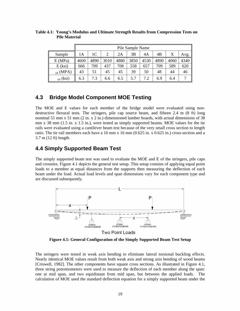
Table 4.1: Young’s Modulus and Ultimate Strength Results from Compression Tests on Pile Material

Pile Sample Name Sample 1A 1C 2 2A 3B 4A 4B X Avg. E (MPa) 4600 4890 3010 4880 3850 4530 4890 4060 4340 E (ksi) 666 709 437 708 558 657 709 589 620

�ult (MPA) 43 51 45 45 39 50 48 44 46 �ult (ksi) 6.3 7.3 6.6 6.5 5.7 7.2 6.9 6.4 7

4.3 Bridge Model Component MOE Testing The MOE and E values for each member of the bridge model were evaluated using non-destructive flexural tests. The stringers, pile cap source beam, and fifteen 2.4 m (8 ft) long nominal 51 mm x 51 mm (2 in. x 2 in.) dimensioned lumber boards, with actual dimensions of 38 mm x 38 mm (1.5 in. x 1.5 in.), were tested as simply supported beams. MOE values for the tie rails were evaluated using a cantilever beam test because of the very small cross section to length ratio. The tie rail members each have a 16 mm x 16 mm (0.625 in. x 0.625 in.) cross-section and a 3.7 m (12 ft) length. 4.4 Simply Supported Beam Test The simply supported beam test was used to evaluate the MOE and E of the stringers, pile caps and crossties. Figure 4.1 depicts the general test setup. This setup consists of applying equal point loads to a member at equal distances from the supports then measuring the deflection of each beam under the load. Actual load levels and span dimensions vary for each component type and are discussed subsequently.

Figure 4.1: General Configuration of the Simply Supported Beam Test Setup

The stringers were tested in weak axis bending to eliminate lateral torsional buckling effects. Nearly identical MOE values result from both weak axis and strong axis bending of wood beams [Criswell, 1982]. The other components have square cross sections. As illustrated in Figure 4.1, three string potentiometers were used to measure the deflection of each member along the span: one at mid span, and two equidistant from mid span, but between the applied loads. The calculation of MOE used the standard deflection equation for a simply supported beam under the

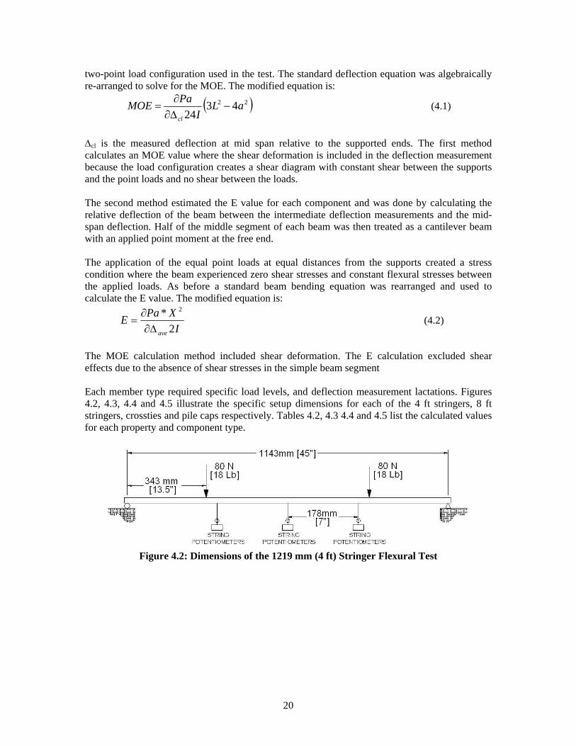
20

two-point load configuration used in the test. The standard deflection equation was algebraically re-arranged to solve for the MOE. The modified equation is:

( )22 4324

aLI

PaMOEcl

−Δ∂∂

= (4.1)

Δcl is the measured deflection at mid span relative to the supported ends. The first method calculates an MOE value where the shear deformation is included in the deflection measurement because the load configuration creates a shear diagram with constant shear between the supports and the point loads and no shear between the loads. The second method estimated the E value for each component and was done by calculating the relative deflection of the beam between the intermediate deflection measurements and the mid-span deflection. Half of the middle segment of each beam was then treated as a cantilever beam with an applied point moment at the free end. The application of the equal point loads at equal distances from the supports created a stress condition where the beam experienced zero shear stresses and constant flexural stresses between the applied loads. As before a standard beam bending equation was rearranged and used to calculate the E value. The modified equation is:

IXPaE

ave 2* 2

Δ∂∂

= (4.2)

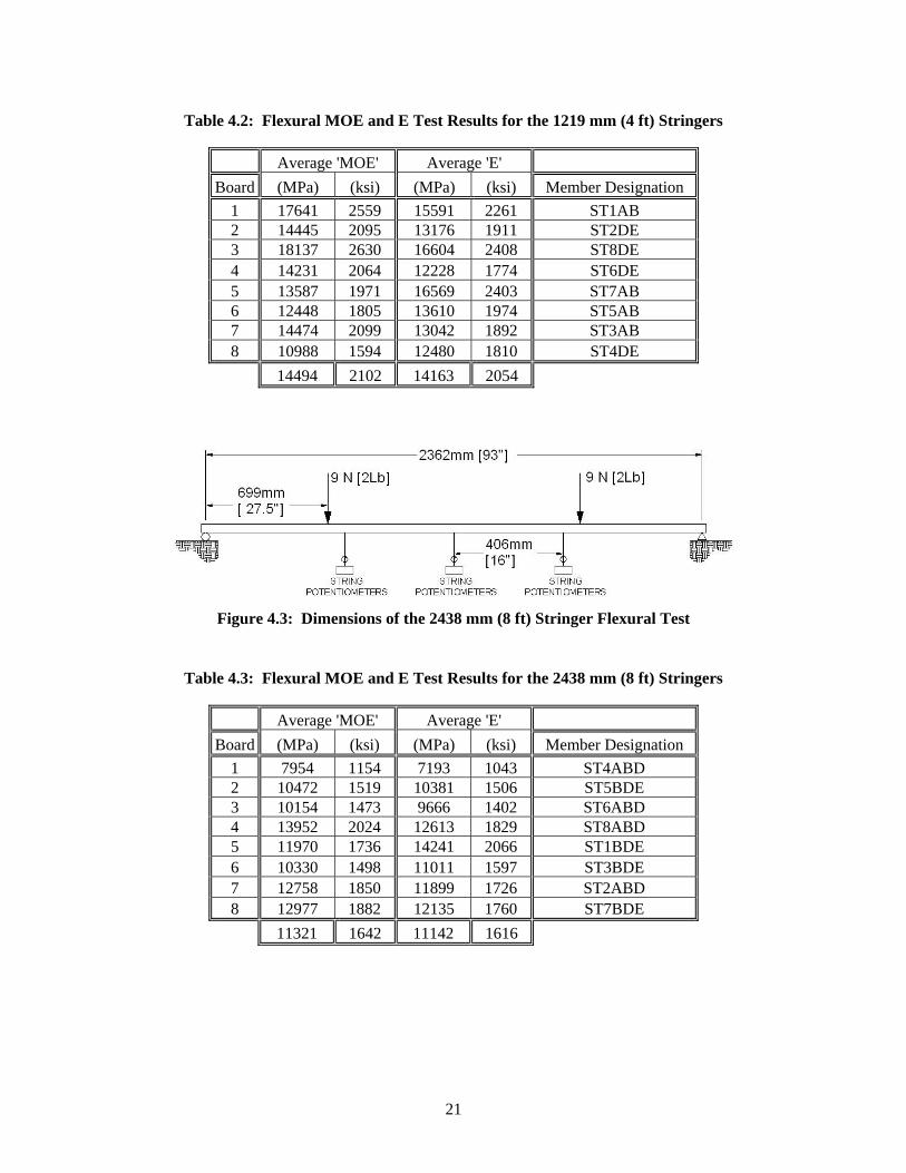
The MOE calculation method included shear deformation. The E calculation excluded shear effects due to the absence of shear stresses in the simple beam segment Each member type required specific load levels, and deflection measurement lactations. Figures 4.2, 4.3, 4.4 and 4.5 illustrate the specific setup dimensions for each of the 4 ft stringers, 8 ft stringers, crossties and pile caps respectively. Tables 4.2, 4.3 4.4 and 4.5 list the calculated values for each property and component type.

Figure 4.2: Dimensions of the 1219 mm (4 ft) Stringer Flexural Test

21

Table 4.2: Flexural MOE and E Test Results for the 1219 mm (4 ft) Stringers

Average 'MOE' Average 'E' Board (MPa) (ksi) (MPa) (ksi) Member Designation

1 17641 2559 15591 2261 ST1AB 2 14445 2095 13176 1911 ST2DE 3 18137 2630 16604 2408 ST8DE 4 14231 2064 12228 1774 ST6DE 5 13587 1971 16569 2403 ST7AB 6 12448 1805 13610 1974 ST5AB 7 14474 2099 13042 1892 ST3AB 8 10988 1594 12480 1810 ST4DE 14494 2102 14163 2054

Figure 4.3: Dimensions of the 2438 mm (8 ft) Stringer Flexural Test

Table 4.3: Flexural MOE and E Test Results for the 2438 mm (8 ft) Stringers


1 7954 1154 7193 1043 ST4ABD 2 10472 1519 10381 1506 ST5BDE 3 10154 1473 9666 1402 ST6ABD 4 13952 2024 12613 1829 ST8ABD 5 11970 1736 14241 2066 ST1BDE 6 10330 1498 11011 1597 ST3BDE 7 12758 1850 11899 1726 ST2ABD 8 12977 1882 12135 1760 ST7BDE 11321 1642 11142 1616

22

Figure 4.4: Dimensions of the 2273 mm (8 ft) Crossties Flexural Test

Table 4.4: Flexural MOE and E Results for the 2273 mm (8 ft) Stringers


1 13925 2020 14545 2110 T1, T18, T35 & T52 2 13591 1971 13883 2014 T9, T22, T36 & T48 3 13004 1886 15192 2203 T23, T37, &T50 4 7154 1038 7346 1065 Not Used (Too Weak) 5 14409 2090 16465 2388 T10, T24, T38 & T51 6 13491 1957 14703 2133 T11, T25 & T39 7 14741 2138 14753 2140 T12, T26 & T40 8 14653 2125 15382 2231 T13, T27 & T41 9 16324 2368 18161 2634 T2, T14, T28 & T42

10 14353 2082 14580 2115 T3, T15, T29 & T43 11 18324 2658 17965 2606 T4, T16, T30 & T44 12 12842 1863 12952 1879 T5, T17, T31, T45 13 11284 1637 10908 1582 T6, T19, T32 & T46 14 14737 2137 13375 1940 T7, T20, T33 & T47 15 14350 2081 15085 2188 T8, T21, T34 & T48

Average 13812 2003 14353 2082

Figure 4.5: Dimensions of the 2997 mm (10 ft) Pile Cap Beam Flexural Test

23

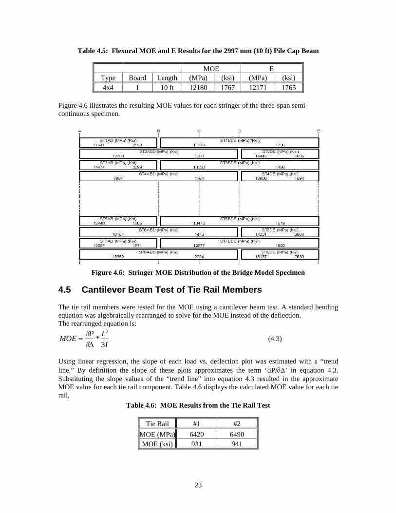
Table 4.5: Flexural MOE and E Results for the 2997 mm (10 ft) Pile Cap Beam

MOE E Type Board Length (MPa) (ksi) (MPa) (ksi) 4x4 1 10 ft 12180 1767 12171 1765

Figure 4.6 illustrates the resulting MOE values for each stringer of the three-span semi-continuous specimen.

Figure 4.6: Stringer MOE Distribution of the Bridge Model Specimen

4.5 Cantilever Beam Test of Tie Rail Members The tie rail members were tested for the MOE using a cantilever beam test. A standard bending equation was algebraically rearranged to solve for the MOE instead of the deflection. The rearranged equation is:

ILPMOE3

*3

Δ=

δδ

(4.3)

Using linear regression, the slope of each load vs. deflection plot was estimated with a “trend line.” By definition the slope of these plots approximates the term ‘dP/δΔ’ in equation 4.3. Substituting the slope values of the “trend line” into equation 4.3 resulted in the approximate MOE value for each tie rail component. Table 4.6 displays the calculated MOE value for each tie rail,

Table 4.6: MOE Results from the Tie Rail Test

Tie Rail #1 #2 MOE (MPa) 6420 6490 MOE (ksi) 931 941

24

All of the beam tests resulted in similar values for the MOE and E value of each member. Having these two methods of measuring each member’s stiffness result in similar values corresponds to very little shear deformation being experienced within these members under load. This was expected because all the members have a very large span-to-depth ratio. Large span-to-depth ratios indicate that a smaller portion of the applied load is resisted by shear stresses.

25

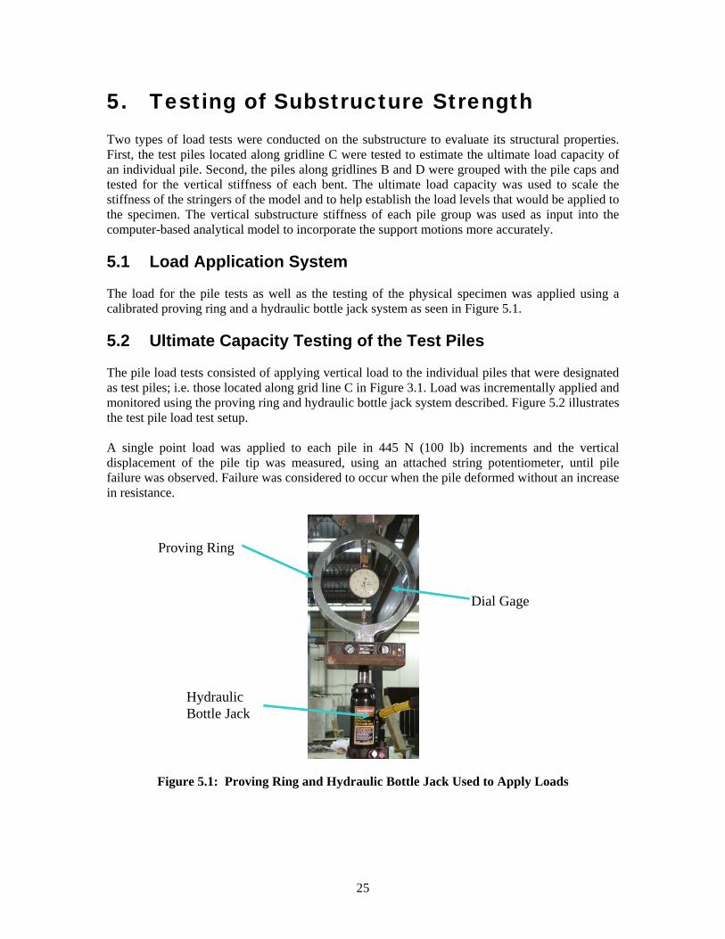
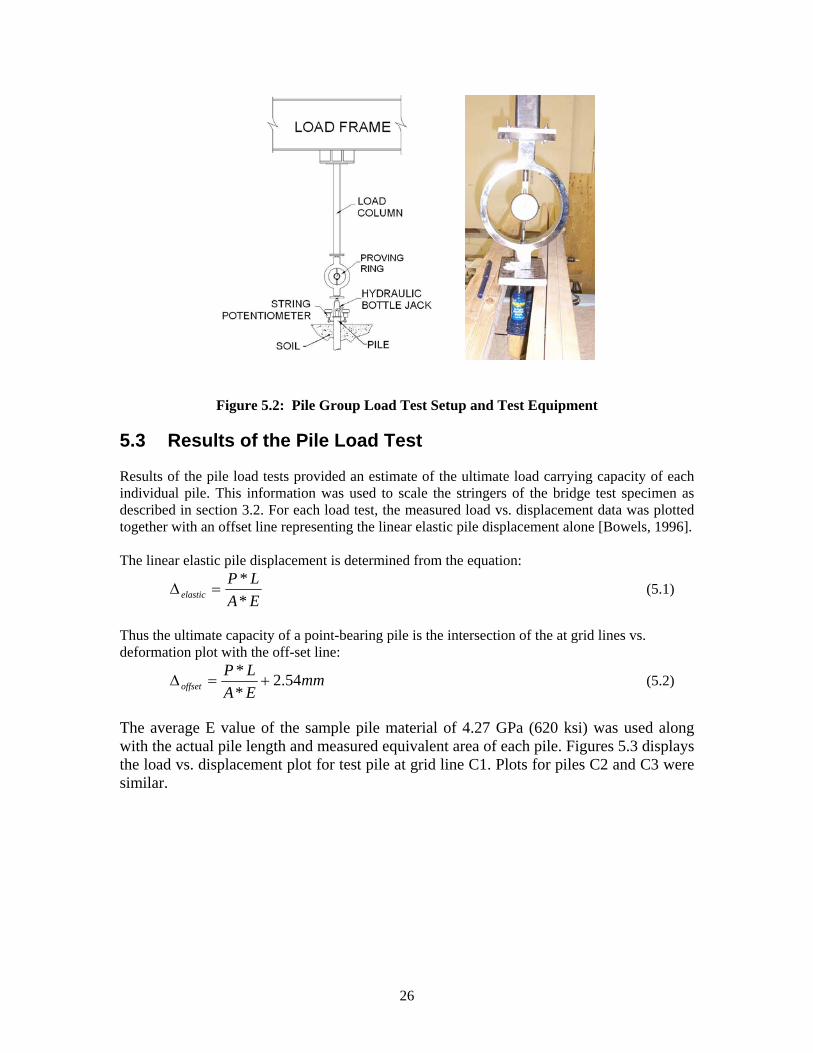
5. Testing of Substructure Strength Two types of load tests were conducted on the substructure to evaluate its structural properties. First, the test piles located along gridline C were tested to estimate the ultimate load capacity of an individual pile. Second, the piles along gridlines B and D were grouped with the pile caps and tested for the vertical stiffness of each bent. The ultimate load capacity was used to scale the stiffness of the stringers of the model and to help establish the load levels that would be applied to the specimen. The vertical substructure stiffness of each pile group was used as input into the computer-based analytical model to incorporate the support motions more accurately. 5.1 Load Application System The load for the pile tests as well as the testing of the physical specimen was applied using a calibrated proving ring and a hydraulic bottle jack system as seen in Figure 5.1. 5.2 Ultimate Capacity Testing of the Test Piles The pile load tests consisted of applying vertical load to the individual piles that were designated as test piles; i.e. those located along grid line C in Figure 3.1. Load was incrementally applied and monitored using the proving ring and hydraulic bottle jack system described. Figure 5.2 illustrates the test pile load test setup. A single point load was applied to each pile in 445 N (100 lb) increments and the vertical displacement of the pile tip was measured, using an attached string potentiometer, until pile failure was observed. Failure was considered to occur when the pile deformed without an increase in resistance.

Figure 5.1: Proving Ring and Hydraulic Bottle Jack Used to Apply Loads

Proving Ring

Hydraulic Bottle Jack

Dial Gage

26

Figure 5.2: Pile Group Load Test Setup and Test Equipment

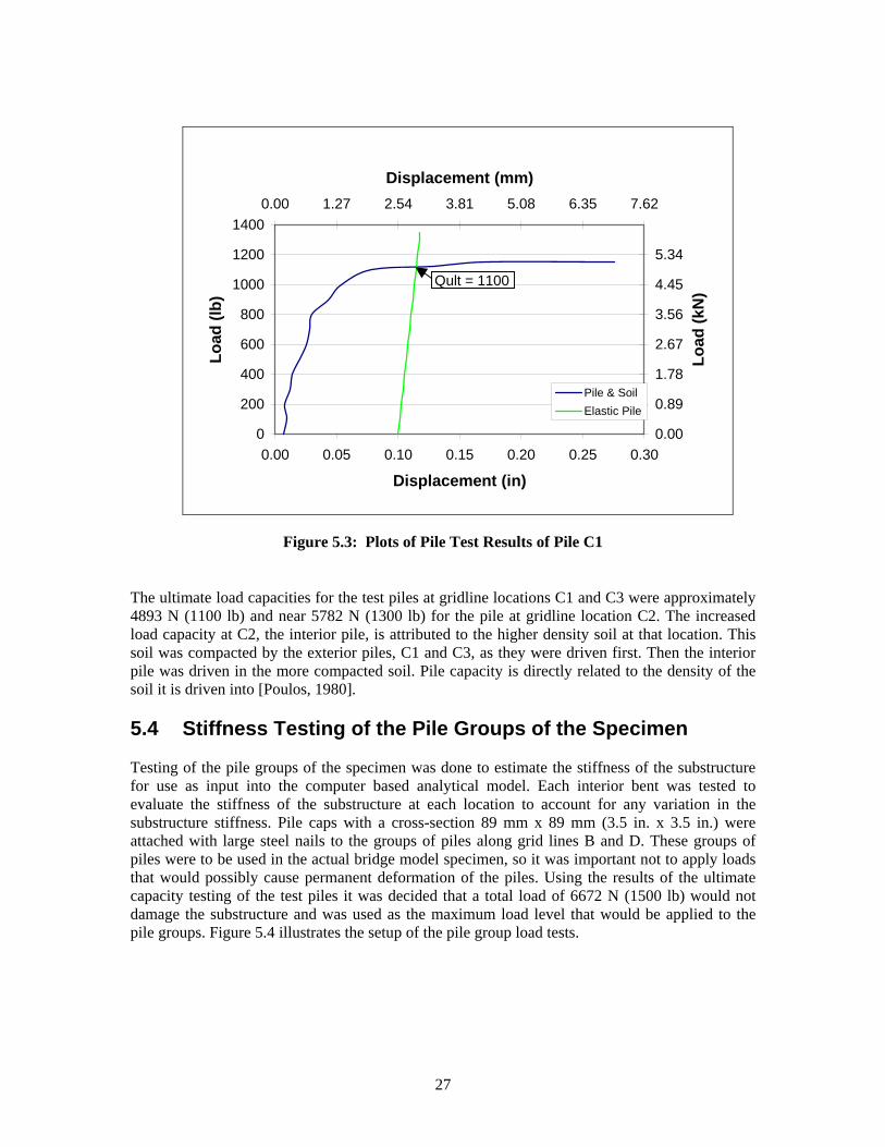
5.3 Results of the Pile Load Test Results of the pile load tests provided an estimate of the ultimate load carrying capacity of each individual pile. This information was used to scale the stringers of the bridge test specimen as described in section 3.2. For each load test, the measured load vs. displacement data was plotted together with an offset line representing the linear elastic pile displacement alone [Bowels, 1996]. The linear elastic pile displacement is determined from the equation:

EALP

elastic **

=Δ (5.1)

Thus the ultimate capacity of a point-bearing pile is the intersection of the at grid lines vs. deformation plot with the off-set line:

mmEALP

offset 54.2**

+=Δ (5.2)

The average E value of the sample pile material of 4.27 GPa (620 ksi) was used along with the actual pile length and measured equivalent area of each pile. Figures 5.3 displays the load vs. displacement plot for test pile at grid line C1. Plots for piles C2 and C3 were similar.

27

0

200

400

600

800

1000

1200

1400

0.00 0.05 0.10 0.15 0.20 0.25 0.30

Displacement (in)

Load

(lb)

0.00

0.89

1.78

2.67

3.56

4.45

5.34

0.00 1.27 2.54 3.81 5.08 6.35 7.62

Displacement (mm)

Load

(kN

)

Pile & SoilElastic Pile

Qult = 1100

Figure 5.3: Plots of Pile Test Results of Pile C1

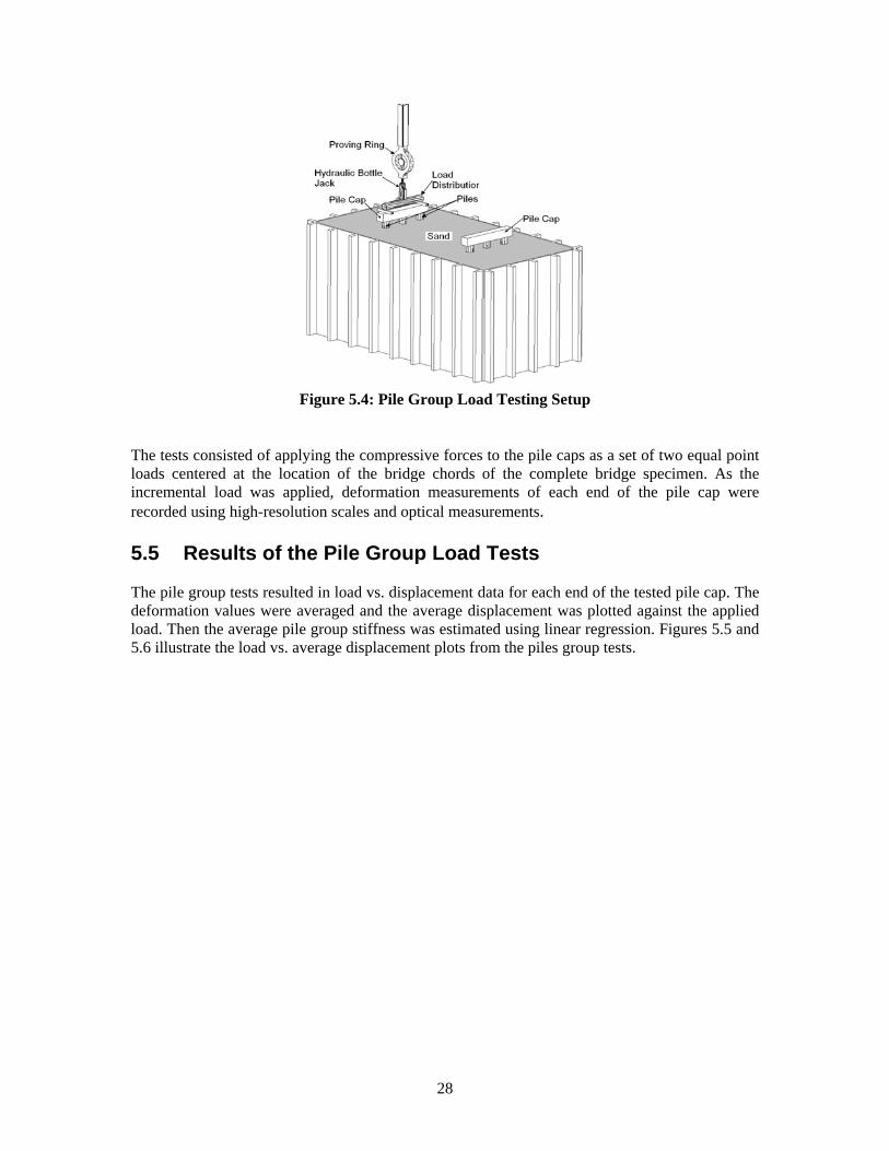
The ultimate load capacities for the test piles at gridline locations C1 and C3 were approximately 4893 N (1100 lb) and near 5782 N (1300 lb) for the pile at gridline location C2. The increased load capacity at C2, the interior pile, is attributed to the higher density soil at that location. This soil was compacted by the exterior piles, C1 and C3, as they were driven first. Then the interior pile was driven in the more compacted soil. Pile capacity is directly related to the density of the soil it is driven into [Poulos, 1980]. 5.4 Stiffness Testing of the Pile Groups of the Specimen Testing of the pile groups of the specimen was done to estimate the stiffness of the substructure for use as input into the computer based analytical model. Each interior bent was tested to evaluate the stiffness of the substructure at each location to account for any variation in the substructure stiffness. Pile caps with a cross-section 89 mm x 89 mm (3.5 in. x 3.5 in.) were attached with large steel nails to the groups of piles along grid lines B and D. These groups of piles were to be used in the actual bridge model specimen, so it was important not to apply loads that would possibly cause permanent deformation of the piles. Using the results of the ultimate capacity testing of the test piles it was decided that a total load of 6672 N (1500 lb) would not damage the substructure and was used as the maximum load level that would be applied to the pile groups. Figure 5.4 illustrates the setup of the pile group load tests.

28

Figure 5.4: Pile Group Load Testing Setup

The tests consisted of applying the compressive forces to the pile caps as a set of two equal point loads centered at the location of the bridge chords of the complete bridge specimen. As the incremental load was applied, deformation measurements of each end of the pile cap were recorded using high-resolution scales and optical measurements. 5.5 Results of the Pile Group Load Tests The pile group tests resulted in load vs. displacement data for each end of the tested pile cap. The deformation values were averaged and the average displacement was plotted against the applied load. Then the average pile group stiffness was estimated using linear regression. Figures 5.5 and 5.6 illustrate the load vs. average displacement plots from the piles group tests.

29

0

300

600

900

1200

1500

1800

0.00 0.05 0.10 0.15Average Displacement (in)

Load

(lb)

0

1334

2669

4003

5338

6672

8007

0 1.27 2.54 3.81

Average Displacement (mm)

Load

(N)

y = 14080x + 181.71

Figure 5.5: Load vs. Average Displacement Plot for Pile Group ‘B’

0

300

600

900

1200

1500

1800

0.00 0.05 0.10Average Displacement (in)

Load

(lb)

0

1334

2669

4003

5338

6672

8007

0 1.27 2.54

Average Displacement (mm)

Load

(N)

y = 20985x + 269.17

Figure 5.6: Load vs. Average Displacement Plot for Pile Group ‘D’

The stiffness values estimated by the linear regression of the average deformation included the stiffness of the wood pile material and the sand that supports all three piles under each group. The stiffness of the sand underneath one pile per bent is needed for input into the computer model. Equivalent spring calculations were used to evaluate the stiffness of the sand under a single pile with the following equations [Thompson, 1998].

LEAK = = Spring constant of axially loaded members (5.1)

When multiple springs are in the system, the stiffness values are combined as follows:

∑= iTotal KK For springs acting parallel to each other (5.2)

30

∑=iTotal KK

11 For springs acting in series to each other (5.3)

Where: K = Spring constant of the system E = Young’s Modulus of the piles A = Cross-sectional area of the piles L = Length of the piles The soil stiffness is assumed to be uniform for each pile group. In this example it was assumed that there was no pile side resistance. From the load vs. average deformation plot of pile cap B the total stiffness is shown to be 2,465 kN/mm (14,080 lb/in.). Assuming that the pile cap is rigid, the total stiffness is divided by 3 to calculate the stiffness of one pile, alone, and the sand around it. This gives a single pile-sand stiffness of 821.8 kN/mm (4693 lb/in.). The stiffness of the sand beneath one pile was calculated as:

BsandBsand

BsandBsandpiletotal

KmmkNKmm

mmGPammkN

KLEAKKK

−−

−−

+=+=

+=+=

1/2367

11

10163161*27.4

1/8.821

1

11111

2

mmkNK Bsand /875=∴ − (5000 lb/in)

Figure 5.7 graphically illustrates the equivalent spring calculations.

Figure 5.7: Equivalent Spring Approximation for Pile Group Testing

Conducting similar calculations estimated the sand stiffness underneath pile cap ‘D’ to be:

mmkNK Dsand /1565=− (9000 lb/in). 5.6 Alternative Method to Calculate Substructure Stiffness Because of the inability to conduct load tests on isolated pile bents in the field, an alternative method of calculating the substructure stiffness was investigated. This method uses test data from the load testing of the complete bridge specimen, analytical results from an AxisVM computer model and additional equivalent spring calculations. The test data and AxisVM analytical results were used to approximate the specimen as two springs acting in parallel.

31

The load testing data used were the maximum vertical displacements of pile caps B and D. These data were taken from load test 4 (described in detail in section 6.6), and from a similar load test conducted over pile cap D. Load test #4 consisted of applying a load directly over pile cap B and measuring the complete specimen’s behavior. The calculation of the sand stiffness under pile cap B follows as an example of this method. From Load Test 4, under the maximum load of 6672 N (1500 lb), the end displacement of pile cap B was measured to be 2 mm (0.095 in.). F = KspecimenΔ = 6672 N = Kspecimen (2 mm) ∴Kspecimen = 3336 kN/mm From the preliminary AxisVM model, a 6672 N (1500 lb) load caused the unsupported pile cap B to displace 19 mm (0.722 in.) thus: F = KAxisVM Δ = 6672 N = KAxisVM (19 mm) ∴KAxisVM = 351 N/mm Equation 5.2 was used to calculate the stiffness provided by the piles and sand directly under the applied loading. mmNK BSand /5.851@ =∴ (4862 lb/in) A similar calculation was performed for the sand under pile cap D. This test resulted in pile cap D deflecting 2 mm (0.06 in.) under a 6672 N (1500 lb) load. The calculation resulted with KSand@D = 1487 N/mm (8494 lb/in). The stiffness values resulting from this method are within 5% of the measured stiffness values (875 N/mm & 1565 N/mm, respectively) from the pile group tests.

32

6. Testing of Bridge Model Specimen 6.1 Measurement Method Optical measurements were used instead of electronic string potentiometers or LVDT’s because of the large number of measurement points located along the measured chord. These optical measurements were made using a Leica NA2 auto-level and self-fabricated precision scales placed on the bridge and on stationary reference locations. 6.2 Leica NA2 Auto-Level and Leica GMP3 Optical Micrometer The Leica NA2 auto-level has a 32x magnification and an accuracy of 0.3 mm, with a minimum focal length of 1.6 m. This level was used together with a Leica GMP3 optical micrometer, which attaches to the NA2 auto-level and doubles the magnification and increases the measurement accuracy. The auto-level and micrometer setup was supported by a standard surveying tripod. Figure 6.1 shows the Leica equipment used.

Figure 6.1: Leica NA2 Auto Level and Leica GMP3 Optical Micrometer

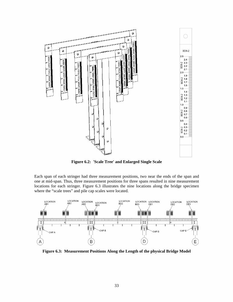
6.3 Measurement Devices Eighty scales with 0.254 mm (0.01 in.) graduations were used to measure the deflection of the specimen chord. The scales were suspended from lightweight steel T-shaped towers in pairs at 40 locations along the chord; 36 along the stringer plies and 4 on the ends of each pile cap. One scale was attached to each end of the T shape; the scales were allowed to rotate freely relative to the T tower. These towers were attached to the specimen with small nails. Each ply of the chord had nine towers attached. The towers were oriented the same distance along the specimen as neighboring plies, resulting in nine lines of four towers along the specimen. To prevent the layered scales from blocking the optical measurement, the width of the T towers increased for each ply from 51 mm, 76 mm, 102 mm and 127 mm (2 in. to 3 in., 4 in. and 5 in.) for the outer ply inward. Each group of four towers was referred to as a “scale tree” because of their appearance. Figure 6.2 illustrates a “scale tree” and an enlarged single scale.

33

Figure 6.2: 'Scale Tree' and Enlarged Single Scale

Each span of each stringer had three measurement positions, two near the ends of the span and one at mid-span. Thus, three measurement positions for three spans resulted in nine measurement locations for each stringer. Figure 6.3 illustrates the nine locations along the bridge specimen where the “scale trees” and pile cap scales were located.

Figure 6.3: Measurement Positions Along the Length of the physical Bridge Model

34

Position 1 of each span was located 25 mm (1 in.) north of the southern pile cap of that span, position 2 was at mid span, and position 3 was 25 mm (1 in.) south of the northern pile cap. The spacing is the same for all three spans and all four stringer plies. Each scale is labeled according to which span, span position, and ply they are on and which side of the tower they are on. An example label for the south side, mid-span scale on the middle span of the outer most ply is: BD8-2S because it is located in span BD on stringer ply 8, at position 2, and attached to the south side of the T tower. The scales suspended on the pile caps are designated by the gridline the cap is on and which side they are suspended on. Thus Cap A-N corresponds to the scale on pile cap A attached to the north side. Although the labeling system is intricate it was necessary to identify all 80 scales. Hanging the scales in pairs from the T towers allowed the deflection of the specimen to be calculated as the average change in scale readings at each location with a negative value corresponding to downward deflection. 6.4 Measurement Recording Because of the large number of scales and measurement points it was necessary to have multiple locations to set up the auto-level to allow clear viewing of every scale. Figure 6.4 illustrates the positions of the auto-level locations that were used relative to the model bridge specimen. To minimize the duration of each load test, three locations of the auto-level were used. One location was near the south end of the specimen, one was near the north end of the specimen; and one was near the center of the specimen. The locations were identified as locations 1, 2, and 3 respectively. Location 3 was approximately 8 in. lower to the ground than the others because of the drastic elevation change between the stringer scales and the pile cap scales.

Figure 6.4: Plan View of the 3 Auto-Level Locations Used

Location 1 allowed for reading all hanging scales at the south end, location 2 allowed for reading all hanging scales at the north end and location 3 allowed for reading all of the pile cap scales.

35

6.5 Load Application Load was applied to the specimen using the hydraulic bottle jack and proving ring as described in section 5.1. Also a load-distributing apparatus was between the bottle jack and the test specimen. The loading setup that was used is illustrated in Figure 6.56.5. The load distributor consisted of a 76 mm (3 in.) diameter steel pipe with a 102 mm (4 in.) square by 6 mm (0.25 in.) flat plate welded on at mid length of the pipe to allow the bottle jack to set vertically. The steel pipe was supported by two solid steel bars that were 19 mm (3/4 in.) square and 203 mm (8 in.) long. These steel bars were centered above each chord and rested on the three crossties nearest to the load location. This was done to distribute the load in a similar manner as the steel train rails of field bridges. It was also assumed that the load distributor evenly distributed the load between the two bridge chords. Figure 6.6 illustrates how the load is distributed between the crossties of the specimen.

Figure 6.5: 3D Rendering and Photo of the Specimen Load Test Setup

Figure 6.6: Diagram of the Load Distribution to the Crossties

The loading system allowed for the natural distribution of load to occur through the crossties and stringers as well as for the possible uneven rotation of each chord.

36

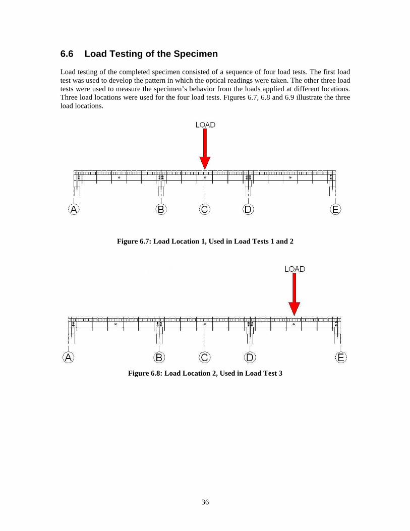
6.6 Load Testing of the Specimen Load testing of the completed specimen consisted of a sequence of four load tests. The first load test was used to develop the pattern in which the optical readings were taken. The other three load tests were used to measure the specimen’s behavior from the loads applied at different locations. Three load locations were used for the four load tests. Figures 6.7, 6.8 and 6.9 illustrate the three load locations.

Figure 6.7: Load Location 1, Used in Load Tests 1 and 2

Figure 6.8: Load Location 2, Used in Load Test 3

37

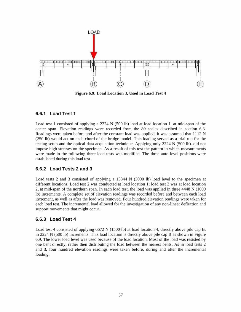
Figure 6.9: Load Location 3, Used in Load Test 4

6.6.1 Load Test 1 Load test 1 consisted of applying a 2224 N (500 lb) load at load location 1, at mid-span of the center span. Elevation readings were recorded from the 80 scales described in section 6.3. Readings were taken before and after the constant load was applied, it was assumed that 1112 N (250 lb) would act on each chord of the bridge model. This loading served as a trial run for the testing setup and the optical data acquisition technique. Applying only 2224 N (500 lb). did not impose high stresses on the specimen. As a result of this test the pattern in which measurements were made in the following three load tests was modified. The three auto level positions were established during this load test. 6.6.2 Load Tests 2 and 3 Load tests 2 and 3 consisted of applying a 13344 N (3000 lb) load level to the specimen at different locations. Load test 2 was conducted at load location 1; load test 3 was at load location 2, at mid-span of the northern span. In each load test, the load was applied in three 4448 N (1000 lb) increments. A complete set of elevation readings was recorded before and between each load increment, as well as after the load was removed. Four hundred elevation readings were taken for each load test. The incremental load allowed for the investigation of any non-linear deflection and support movements that might occur. 6.6.3 Load Test 4 Load test 4 consisted of applying 6672 N (1500 lb) at load location 4, directly above pile cap B, in 2224 N (500 lb) increments. This load location is directly above pile cap B as shown in Figure 6.9. The lower load level was used because of the load location. Most of the load was resisted by one bent directly, rather then distributing the load between the nearest bents. As in load tests 2 and 3, four hundred elevation readings were taken before, during and after the incremental loading.

38

7. Description of Computer Based Bridge Model

The goal of this research was to develop a computer-based analytical model to predict the behavior of a timber trestle railroad bridge with consideration of the support movement and irregular small gaps between crossties and stringer members. Commercially available software was used to create the analytical model. The chosen software has been developed and refined through the efforts of many professionals. The algorithms and architecture of the software have been demonstrated to be accurate and reliable. 7.1 AxisVM AxisVM software was used to develop the analytical computer bridge model for this research. Developed by InterCAD Kft, AxisVM is a finite-element-based program designed for visual modeling for structural analysis. A detailed description of the software is available at www.AxisVM.com [InterCAD Kft, 2004]. “Beam,” “nodal support,” “rigid,” “spring,” “gap,” and “link” elements were used to develop the analytical model of the bridge specimen. 7.2 Description of Utilized Elements Beam elements are used to model frame structures. Beams are two-node, straight elements with constant cross-section properties along their length. A maximum of three translational and three rotational degrees of freedom (DOF) are defined for each node of the elements as illustrated in Figure 7.1.

Figure 7.1: Conceptual Image of a Beam Element and the Possible DOFs

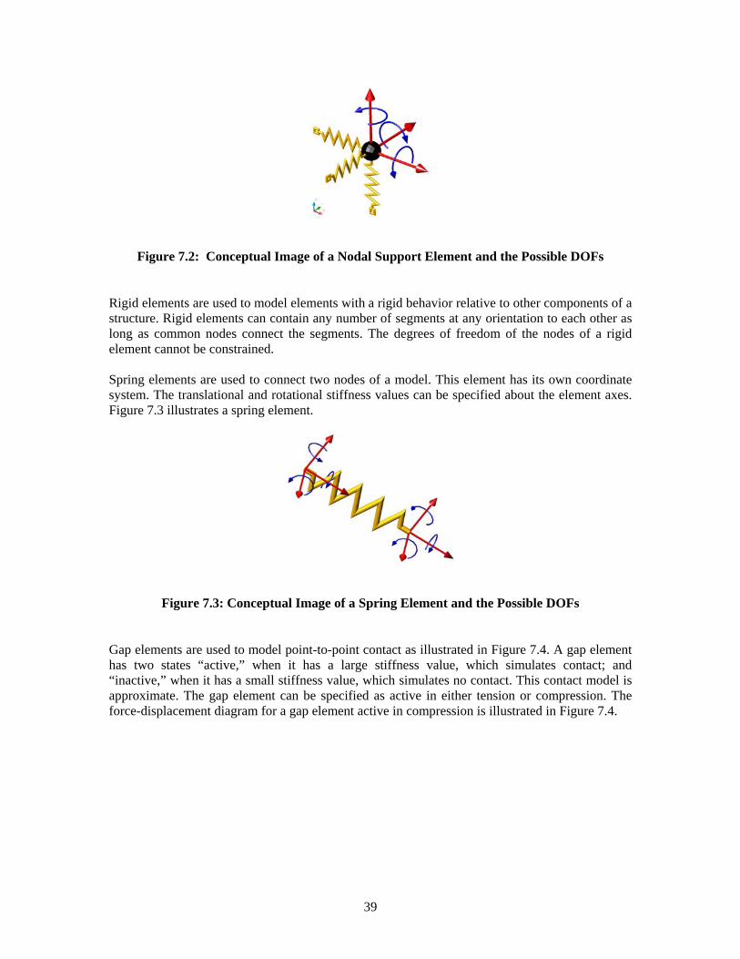
Nodal support elements are used to model point support conditions of a structure. Nodal support elements support nodes where the translational and/or rotational stiffness values can be specified. Figure 7.2 illustrates a nodal support element.

39

Figure 7.2: Conceptual Image of a Nodal Support Element and the Possible DOFs

Rigid elements are used to model elements with a rigid behavior relative to other components of a structure. Rigid elements can contain any number of segments at any orientation to each other as long as common nodes connect the segments. The degrees of freedom of the nodes of a rigid element cannot be constrained. Spring elements are used to connect two nodes of a model. This element has its own coordinate system. The translational and rotational stiffness values can be specified about the element axes. Figure 7.3 illustrates a spring element.

Figure 7.3: Conceptual Image of a Spring Element and the Possible DOFs

Gap elements are used to model point-to-point contact as illustrated in Figure 7.4. A gap element has two states “active,” when it has a large stiffness value, which simulates contact; and “inactive,” when it has a small stiffness value, which simulates no contact. This contact model is approximate. The gap element can be specified as active in either tension or compression. The force-displacement diagram for a gap element active in compression is illustrated in Figure 7.4.

40

Figure 7.4: Gap Element Active in Compression with Associated Force-Displacement Diagram

The gap element is a nonlinear element because as displacement of a structure occurs the contact conditions which the gap models can change. As the gap transitions between its active and inactive state the utilized stiffness value also changes drastically, increasing if the gap becomes active. Because of this inherent non-linearity, an iterative solution process is used. A link element connects two nodes and has six stiffness components that are concentrated at an interface between the two connected nodes. The interface’s position can be entered relative to one node that is considered as a reference. The stiffness components are defined in the global coordinate system. Assigning a zero value to a stiffness component indicates that the corresponding force or displacement will not be transferred from one node to the other. Figure 7.5 illustrates a link element.

Figure 7.5: Conceptual Image of a Link Element and the Possible DOFs

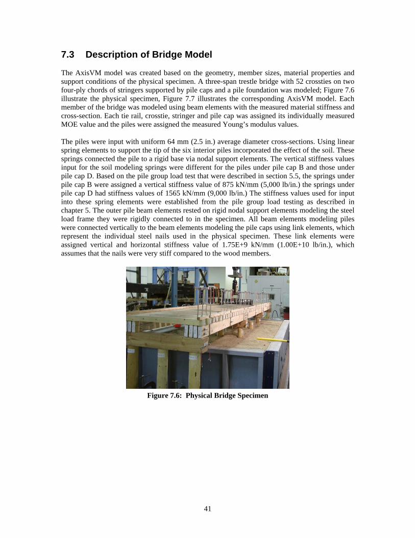
41

7.3 Description of Bridge Model The AxisVM model was created based on the geometry, member sizes, material properties and support conditions of the physical specimen. A three-span trestle bridge with 52 crossties on two four-ply chords of stringers supported by pile caps and a pile foundation was modeled; Figure 7.6 illustrate the physical specimen, Figure 7.7 illustrates the corresponding AxisVM model. Each member of the bridge was modeled using beam elements with the measured material stiffness and cross-section. Each tie rail, crosstie, stringer and pile cap was assigned its individually measured MOE value and the piles were assigned the measured Young’s modulus values. The piles were input with uniform 64 mm (2.5 in.) average diameter cross-sections. Using linear spring elements to support the tip of the six interior piles incorporated the effect of the soil. These springs connected the pile to a rigid base via nodal support elements. The vertical stiffness values input for the soil modeling springs were different for the piles under pile cap B and those under pile cap D. Based on the pile group load test that were described in section 5.5, the springs under pile cap B were assigned a vertical stiffness value of 875 kN/mm (5,000 lb/in.) the springs under pile cap D had stiffness values of 1565 kN/mm (9,000 lb/in.) The stiffness values used for input into these spring elements were established from the pile group load testing as described in chapter 5. The outer pile beam elements rested on rigid nodal support elements modeling the steel load frame they were rigidly connected to in the specimen. All beam elements modeling piles were connected vertically to the beam elements modeling the pile caps using link elements, which represent the individual steel nails used in the physical specimen. These link elements were assigned vertical and horizontal stiffness value of 1.75E+9 kN/mm (1.00E+10 lb/in.), which assumes that the nails were very stiff compared to the wood members.

Figure 7.6: Physical Bridge Specimen

42

Figure 7.7: AxisVM Model of the Physical Bridge Specimen

Figure 7.8 illustrates the pile cap configuration of the physical specimen. The pile caps were modeled using a combination of beam elements and rigid elements. Figure 7.9 illustrates the configuration used to model the pile caps.

Figure 7.8: Pile Cap from Physical Specimen

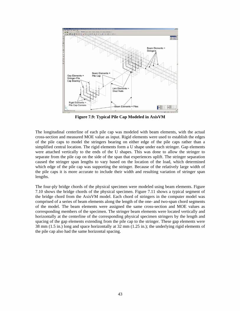
43

Figure 7.9: Typical Pile Cap Modeled in AxisVM

The longitudinal centerline of each pile cap was modeled with beam elements, with the actual cross-section and measured MOE value as input. Rigid elements were used to establish the edges of the pile caps to model the stringers bearing on either edge of the pile caps rather than a simplified central location. The rigid elements form a U shape under each stringer. Gap elements were attached vertically to the ends of the U shapes. This was done to allow the stringer to separate from the pile cap on the side of the span that experiences uplift. The stringer separation caused the stringer span lengths to vary based on the location of the load, which determined which edge of the pile cap was supporting the stringer. Because of the relatively large width of the pile caps it is more accurate to include their width and resulting variation of stringer span lengths. The four-ply bridge chords of the physical specimen were modeled using beam elements. Figure 7.10 shows the bridge chords of the physical specimen. Figure 7.11 shows a typical segment of the bridge chord from the AxisVM model. Each chord of stringers in the computer model was comprised of a series of beam elements along the length of the one- and two-span chord segments of the model. The beam elements were assigned the same cross-section and MOE values as corresponding members of the specimen. The stringer beam elements were located vertically and horizontally at the centerline of the corresponding physical specimen stringers by the length and spacing of the gap elements extending from the pile cap to the stringer. These gap elements were 38 mm (1.5 in.) long and space horizontally at 32 mm (1.25 in.); the underlying rigid elements of the pile cap also had the same horizontal spacing.

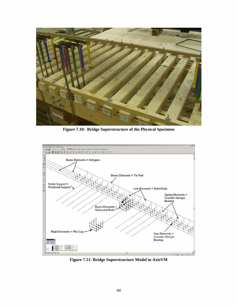
44

Figure 7.10: Bridge Superstructure of the Physical Specimen

Figure 7.11: Bridge Superstructure Model in AxisVM

45

The horizontal bolts connecting the stringers in the specimen were modeled with beam elements with circular cross-section and structural steel material properties. The connection of the outer ply of each specimen chord to the pile caps was modeled using link elements. Each link element represented the vertical bolt through the tie rail, cross tie, stringer and pile cap. The use of link element, where the translational stiffnesses of the interface were specified at a specified distance between the nodes, accounted for the interaction between each wood member. The bolted connections between the stringers, crossties and tie rails were modeled with similar link elements, as were the nailed connections between the tie rail and intermediate crossties. Spring elements were used to model the bearing of the intermediate crossties on the outer stringers where there was no physical connection. The interfaces between the crossties and interior stringers were modeled using gap elements to account for the initial small gaps between many of the crossties and stringers. The spaces were measured in the physical specimen to an accuracy of 0.76 mm (0.03 in.) The measured spaces were input into the corresponding gap elements. The vertical stiffness values of the links and springs were set to correspond to the active vertical stiffness of the gap elements. The software only allows active stiffness values greater than or equal to 1E+6 kN/mm (5.71E+6 lb/in.) to minimize numerical errors from the “penalty” method used in conjunction with the gap elements. Therefore all link elements and spring elements in the superstructure of the AxisVM model were assigned vertical stiffness values of 1E+6 kN/mm (5.71E+6 lb/in.) The horizontal stiffness of the link elements was set to 100 kN/mm (571 lb/in.) The spring elements were assigned zero horizontal stiffness. The need for the links and spring elements to have the same vertical stiffness values as the gap elements comes from their uniform distribution in the specimen. Specifically, after the gaps close, all the vertical connections between the crossties and stringers should have the same stiffness similar to the actual interactions between the crossties and stringers. If the gap elements had a greater vertical stiffness value then the links and springs, they would attract more of the applied load than the links and springs. Although all major components and connection details of the physical specimen are incorporated into the AxisVM model a few additional boundary conditions were necessary to avoid singularities in the numerical model. Therefore one nodal support was added to one end of each series of beam elements that modeled the tie rail. This nodal support provided rotational stiffness about the longitudinal axis of the element only. Each crosstie had a similar nodal support located along the centerline of the entire bridge model. Each interior pile also had a rotational nodal support located at the node that was attached to the spring that modeled the soil stiffness. These nodal supports prevented the members from freely “spinning” about their longitudinal axis. Figure 7.11 includes a typical rotational point support on the crossties. Three versions of the completed AxisVM model were created. Each version of the model differed only by the location and magnitude of the applied loads. These configurations were identified as AxisVM model 2, 3 and 4 to correspond to load tests 2, 3 and 4 respectively. Figure 7.12 shows the application of the load to the physical specimen. The small steel distribution beams were modeled using beam elements with the actual cross-section and structural steel material properties. Figure 7.13 illustrates the application of the loads in one of the AxisVM models.

46

Figure 7.12: Application of the Load to the Physical Specimen

The beam elements used to model the distribution beam spanned three crossties and spring elements with large vertical stiffness of 1.75E+9 kN/mm (1E+10 lb/in.) to simulate the rigid bearing of the steel bar on the cross ties. Zero horizontal stiffness was input for the springs, similar to the physical specimen where only friction forces could have prevented horizontal movement.

Figure 7.13: Typical Application of Point Loads into the AxisVM Model

The assumption of equal load distribution into the two bridge chords was used whereby each point load was set equal to one half of the load increments from the load tests. The point loads were set to 2224 N (500 lb) for AxisVM models 2 and 3, and to 1112 N (250 lb) for AxisVM model 4. To produce corresponding deflection data for the load tests, the load was analytically applied in increments and calculated results for each increment were obtained. Increments of 1, 2 and 3 times the assigned point loads were used when conducting the computer-based analysis and the calculated deflections results were compared to the corresponding load test results.

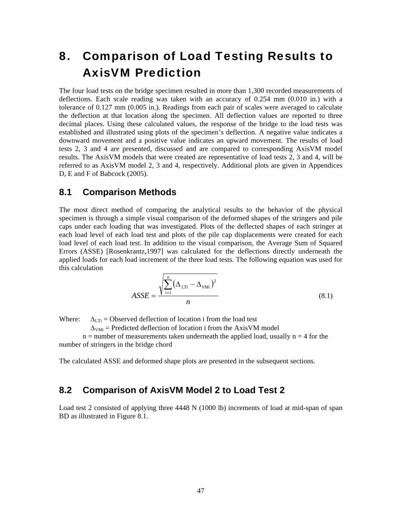
47

8. Comparison of Load Testing Results to AxisVM Prediction

The four load tests on the bridge specimen resulted in more than 1,300 recorded measurements of deflections. Each scale reading was taken with an accuracy of 0.254 mm (0.010 in.) with a tolerance of 0.127 mm (0.005 in.). Readings from each pair of scales were averaged to calculate the deflection at that location along the specimen. All deflection values are reported to three decimal places. Using these calculated values, the response of the bridge to the load tests was established and illustrated using plots of the specimen’s deflection. A negative value indicates a downward movement and a positive value indicates an upward movement. The results of load tests 2, 3 and 4 are presented, discussed and are compared to corresponding AxisVM model results. The AxisVM models that were created are representative of load tests 2, 3 and 4, will be referred to as AxisVM model 2, 3 and 4, respectively. Additional plots are given in Appendices D, E and F of Babcock (2005). 8.1 Comparison Methods The most direct method of comparing the analytical results to the behavior of the physical specimen is through a simple visual comparison of the deformed shapes of the stringers and pile caps under each loading that was investigated. Plots of the deflected shapes of each stringer at each load level of each load test and plots of the pile cap displacements were created for each load level of each load test. In addition to the visual comparison, the Average Sum of Squared Errors (ASSE) [Rosenkrantz,1997] was calculated for the deflections directly underneath the applied loads for each load increment of the three load tests. The following equation was used for this calculation

( )

nASSE

n

iVMiLTi∑

=

Δ−Δ= 1

2

(8.1)

Where: ΔLTi = Observed deflection of location i from the load test ΔVMi = Predicted deflection of location i from the AxisVM model

n = number of measurements taken underneath the applied load, usually n = 4 for the number of stringers in the bridge chord The calculated ASSE and deformed shape plots are presented in the subsequent sections. 8.2 Comparison of AxisVM Model 2 to Load Test 2 Load test 2 consisted of applying three 4448 N (1000 lb) increments of load at mid-span of span BD as illustrated in Figure 8.1.

48

Figure 8.1: Measurement Positions and Load Application for Load Test 2

and AxisVM Model #2

Figure 8.2 illustrates the pile cap displacements for this load test at 13344 N (3000 lb). This figure shows that the AxisVM model predicts the pile cap displacement very closely.

-0.40-0.35-0.30-0.25-0.20-0.15-0.10-0.050.000.05

0 12 24 36 48 60 72 84 96 108 120 132 144

Distance Along Bridge (in)

Def

lect

ion

(in)

-10.16-8.89-7.62-6.35-5.08-3.81-2.54-1.270.001.27

0 305 610 914 1219 1524 1829 2134 2438 2743 3048 3353 3658

Distance Along Bridge (mm)

Def

lect

ion

(mm

)AxisVM Results Test Results

13344 N

Figure 8.2: Deformed Shape of the Pile Caps Under 13344 N (3000 lb) of Load Test 2

Figures 8.3, 8.4, 8.5 and 8.6 illustrate both the observed and predicted deflected shapes of stringers 5, 6, 7 and 8, respectively, for the 13344 N (3000 lb) load level of load test 2. The predicted deflection for stringer 5 is nearly identical to that observed in the load test, as shown in Figure 8.3. The AxisVM model over estimates the deflection of stringers 7 and 8 near pile cap D by more than 1 mm and under estimates the mid-span deflection for those same stringers by the same margin. However, Figures 8.2, 8.3, 8.4, 8.5 and 8.6 illustrate that the AxisVM model predicted the deflections reasonably well and in all cases the predictions display very similar behavior to those observed in this load test. Plots of the deformed shape of both the stringers and pile caps at the two lower load levels are provided in Appendix F of Babcock (2005) and show similar comparisons.

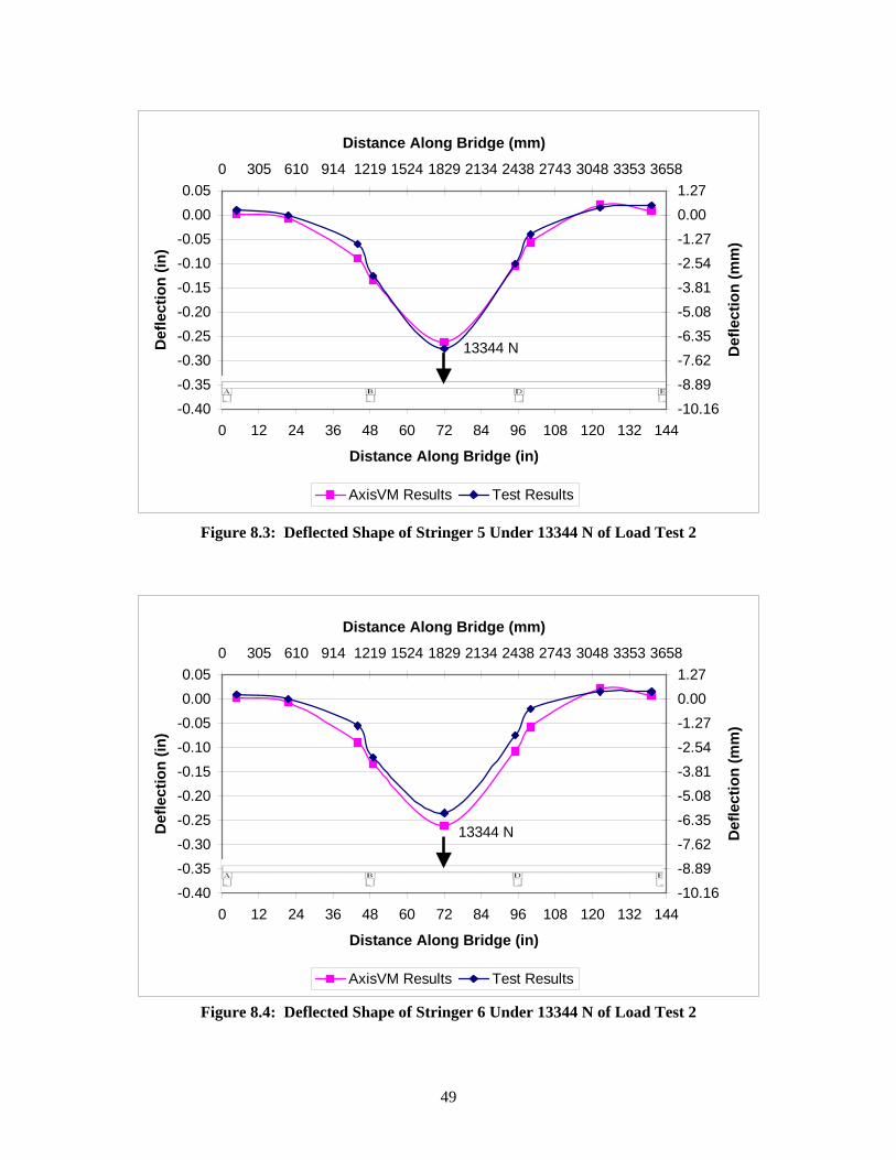
49

-0.40-0.35-0.30-0.25-0.20-0.15-0.10-0.050.000.05

0 12 24 36 48 60 72 84 96 108 120 132 144


Def

lect

ion

(in)

-10.16-8.89-7.62-6.35-5.08-3.81-2.54-1.270.001.27

0 305 610 914 1219 1524 1829 2134 2438 2743 3048 3353 3658


Def

lect

ion

(mm

)

AxisVM Results Test Results

13344 N

Figure 8.3: Deflected Shape of Stringer 5 Under 13344 N of Load Test 2

-0.40-0.35-0.30-0.25-0.20-0.15-0.10-0.050.000.05

0 12 24 36 48 60 72 84 96 108 120 132 144


Def

lect

ion

(in)

-10.16-8.89-7.62-6.35-5.08-3.81-2.54-1.270.001.27

0 305 610 914 1219 1524 1829 2134 2438 2743 3048 3353 3658


Def

lect

ion

(mm

)


13344 N


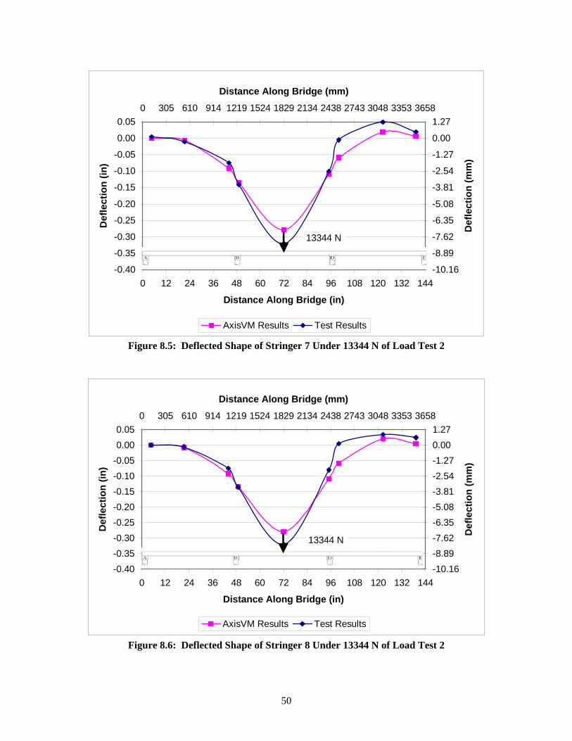
50

-0.40

-0.35

-0.30

-0.25

-0.20

-0.15

-0.10

-0.05

0.00

0.05

0 12 24 36 48 60 72 84 96 108 120 132 144


Def

lect

ion

(in)

-10.16

-8.89

-7.62

-6.35

-5.08

-3.81

-2.54

-1.27

0.00

1.270 305 610 914 1219 1524 1829 2134 2438 2743 3048 3353 3658


Def

lect

ion

(mm

)


13344 N


-0.40-0.35-0.30-0.25-0.20-0.15-0.10-0.050.000.05

0 12 24 36 48 60 72 84 96 108 120 132 144


Def

lect

ion

(in)

-10.16-8.89-7.62-6.35-5.08-3.81-2.54-1.270.001.27

0 305 610 914 1219 1524 1829 2134 2438 2743 3048 3353 3658


Def

lect

ion

(mm

)


13344 N


51

Table 8.1 lists the calculated ASSE value for the mid-span deflections of stringers 5, 6, 7 and 8 for all three load levels of this load test comparison.

Table 8.1: ASSE Value for Load Test 2

Load Level ASSE

4448 N 5.43% 8896 N 4.55%

13344 N 5.17% The above table shows that the ASSE value for all three load levels is approximately 5 percent. This measure indicates that the AxisVM model predicted the mid-span deflection directly under the load to within approximately 5 percent of the observed deflection from the physical load testing of the specimen under all three load level increments. 8.3 Comparison of AxisVM Model 3 to Load Test 3 Load test 3 consisted of applying three 4448 N (1000 lb) increments of load at mid-span of span DE as illustrated in Figure 8.7.

Figure 8.7: Measurement Positions and Load Application for Load Test 3 and Axis VM Model 3

Figure 8.8 illustrates the pile cap displacements for this load test at 13344 N (3000 lb). This figure shows that the AxisVM model predicts the pile cap displacement within 1.27 mm (0.05 in.).

52

-0.40-0.35-0.30-0.25-0.20-0.15-0.10-0.050.000.05

0 12 24 36 48 60 72 84 96 108 120 132 144


Def

lect

ion

(in)

-10.16-8.89-7.62-6.35-5.08-3.81-2.54-1.270.001.27

0 305 610 914 1219 1524 1829 2134 2438 2743 3048 3353 3658


Def

lect

ion

(mm

)


13344 N

Figure 8.8: Deformed Shape of the Pile Caps Under 13344 N of Load Test 3 Figures 8.9, 8.10, 8.11 and 8.12 illustrate both the observed and predicted deflected shapes of stringers 5, 6, 7 and 8, respectively, for the 13344 N (3000 lb) load level of Load Test 3. The predicted maximum deflection for stringer 5 is approximately 0.76 mm (0.03 in.) less than what was observed in the load test as seen in Figure 10.9. The AxisVM model over estimates the deflection of stringer 7. Figures 8.8, 8.9, 8.10, 8.11 and 8.12 illustrate that the AxisVM model predicted the deflections reasonably well and in all cases the predictions display very similar behavior to those observed in this load test. Plots of the deformed shape of both the stringers and pile caps at the two lower load levels are provided in Appendix F of Babcock (2005), and show similar comparisons.

53

-0.40

-0.35

-0.30

-0.25

-0.20

-0.15

-0.10

-0.05

0.00

0.05

0 12 24 36 48 60 72 84 96 108 120 132 144


Def

lect

ion

(in)

-10.16

-8.89

-7.62

-6.35

-5.08

-3.81

-2.54

-1.27

0.00

1.270 305 610 914 1219 1524 1829 2134 2438 2743 3048 3353 3658


Def

lect

ion

(mm

)


13344 N


-0.40

-0.35

-0.30

-0.25

-0.20

-0.15

-0.10

-0.05

0.00

0.05

0 12 24 36 48 60 72 84 96 108 120 132 144


Def

lect

ion

(in)

-10.16

-8.89

-7.62

-6.35

-5.08

-3.81

-2.54

-1.27

0.00

1.270 305 610 914 1219 1524 1829 2134 2438 2743 3048 3353 3658


Def

lect

ion

(mm

)


13344 N


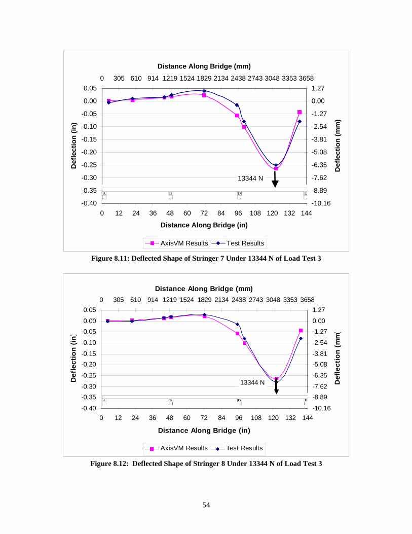
54

-0.40

-0.35

-0.30

-0.25

-0.20

-0.15

-0.10

-0.05

0.00

0.05

0 12 24 36 48 60 72 84 96 108 120 132 144


Def

lect

ion

(in)

-10.16

-8.89

-7.62

-6.35

-5.08

-3.81

-2.54

-1.27

0.00

1.270 305 610 914 1219 1524 1829 2134 2438 2743 3048 3353 3658


Def

lect

ion

(mm

)


13344 N


-0.40

-0.35-0.30

-0.25

-0.20-0.15

-0.10

-0.050.00

0.05

0 12 24 36 48 60 72 84 96 108 120 132 144


Def

lect

ion

(in)

-10.16

-8.89-7.62

-6.35

-5.08-3.81

-2.54

-1.270.00

1.270 305 610 914 1219 1524 1829 2134 2438 2743 3048 3353 3658


Def

lect

ion

(mm

)


13344 N


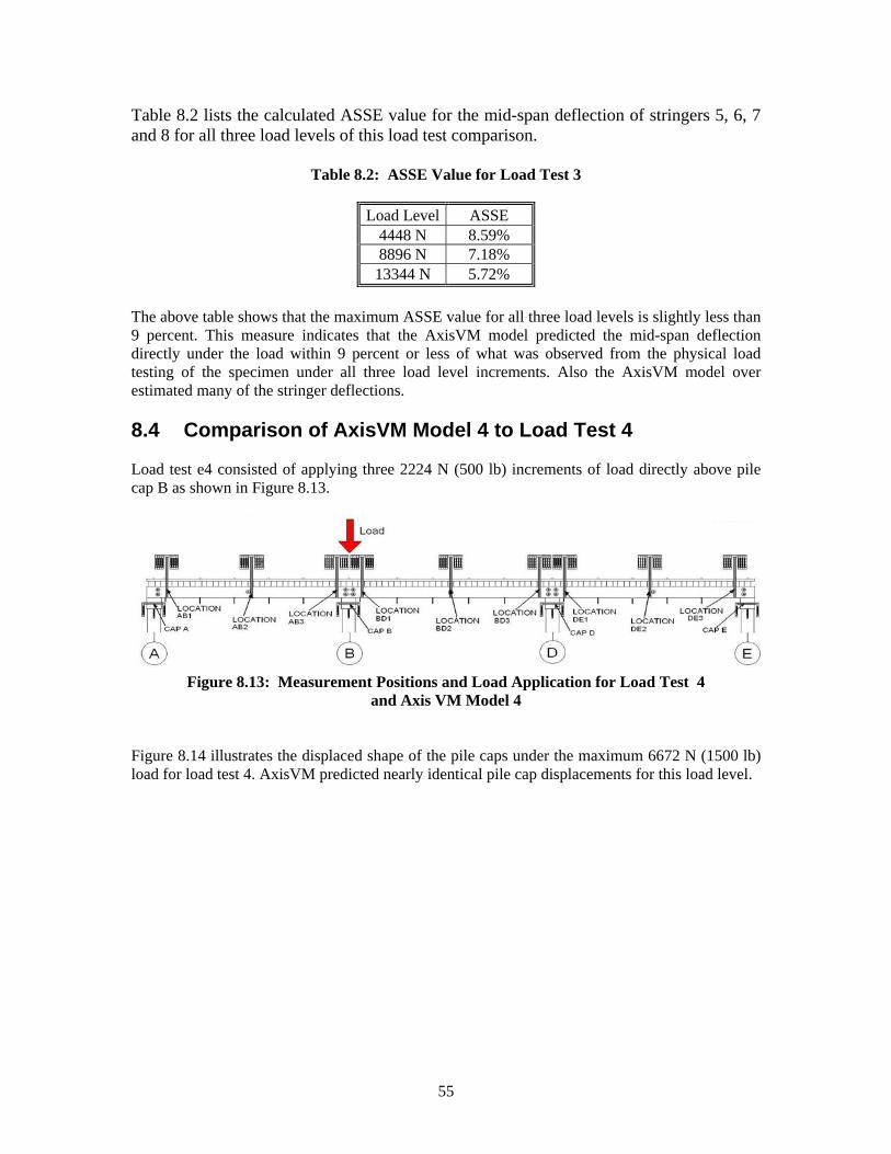
55

Table 8.2 lists the calculated ASSE value for the mid-span deflection of stringers 5, 6, 7 and 8 for all three load levels of this load test comparison.


Load Level ASSE 4448 N 8.59% 8896 N 7.18%

13344 N 5.72% The above table shows that the maximum ASSE value for all three load levels is slightly less than 9 percent. This measure indicates that the AxisVM model predicted the mid-span deflection directly under the load within 9 percent or less of what was observed from the physical load testing of the specimen under all three load level increments. Also the AxisVM model over estimated many of the stringer deflections. 8.4 Comparison of AxisVM Model 4 to Load Test 4 Load test e4 consisted of applying three 2224 N (500 lb) increments of load directly above pile cap B as shown in Figure 8.13.

Figure 8.13: Measurement Positions and Load Application for Load Test 4 and Axis VM Model 4

Figure 8.14 illustrates the displaced shape of the pile caps under the maximum 6672 N (1500 lb) load for load test 4. AxisVM predicted nearly identical pile cap displacements for this load level.

56

-0.40

-0.35

-0.30

-0.25

-0.20

-0.15

-0.10

-0.05

0.00

0.05

0 12 24 36 48 60 72 84 96 108 120 132 144


Def

lect

ion

(in)

-10.16

-8.89

-7.62

-6.35

-5.08

-3.81

-2.54

-1.27

0.00

1.270 305 610 914 1219 1524 1829 2134 2438 2743 3048 3353 3658


Def

lect

ion

(mm

)


6672 N

Figure 8.14: Deformed Shape of the Pile Caps Under 6672 N of Load Test 4 Figures 8.15, 8.16, 8.17 and 8.18 illustrate both the observed and predicted deflected shapes of stringers 5, 6, 7 and 8, respectively, for the 6672 N (1500 lb) load level of load test 4. The predicted deflections for all four stringers are very similar to the observed deflections observed from the specimen. Plots of the deformed shape of both the stringers and pile caps at the two lower load levels are provided in Appendix F of Babcock (2005), and show similar comparisons. The AxisVM predicted deflected shapes for the lower levels also match extremely well with the observed data.

57

-0.40

-0.35

-0.30

-0.25

-0.20

-0.15

-0.10

-0.05

0.00

0.05

0 12 24 36 48 60 72 84 96 108 120 132 144


Def

lect

ion

(in)

-10.16

-8.89

-7.62

-6.35

-5.08

-3.81

-2.54

-1.27

0.00

1.270 305 610 914 1219 1524 1829 2134 2438 2743 3048 3353 3658


Def

lect

ion

(mm

)


6672 N


-0.40

-0.35

-0.30

-0.25

-0.20

-0.15

-0.10

-0.05

0.00

0.05

0 12 24 36 48 60 72 84 96 108 120 132 144


Def

lect

ion

(in)

-10.16

-8.89

-7.62

-6.35

-5.08

-3.81

-2.54

-1.27

0.00

1.270 305 610 914 1219 1524 1829 2134 2438 2743 3048 3353 3658


Def

lect

ion

(mm

)


6672 N


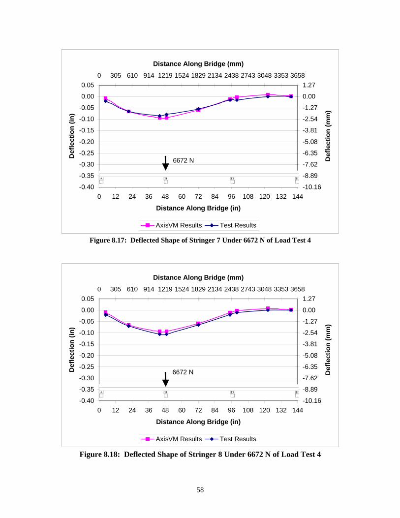
58

-0.40

-0.35

-0.30

-0.25

-0.20

-0.15

-0.10

-0.05

0.00

0.05

0 12 24 36 48 60 72 84 96 108 120 132 144


Def

lect

ion

(in)

-10.16

-8.89

-7.62

-6.35

-5.08

-3.81

-2.54

-1.27

0.00

1.270 305 610 914 1219 1524 1829 2134 2438 2743 3048 3353 3658


Def

lect

ion

(mm

)


6672 N


-0.40

-0.35

-0.30

-0.25

-0.20

-0.15

-0.10

-0.05

0.00

0.05

0 12 24 36 48 60 72 84 96 108 120 132 144


Def

lect

ion

(in)

-10.16

-8.89

-7.62

-6.35

-5.08

-3.81

-2.54

-1.27

0.00

1.270 305 610 914 1219 1524 1829 2134 2438 2743 3048 3353 3658


Def

lect

ion

(mm

)


6672 N


59

Table 8.3 lists the calculated ASSE value for the mid-span deflection for all three load levels of this load test comparison.


Load Level ASSE 2224 N 11.43% 4448 N 10.01% 6672 N 1.04%

The ASSE values for first two load levels are higher than expected. The 6672 N (1500 lb) load level has an extremely low ASSE value, which correlates well with the visual comparison. The noticeable variation in the ASSE values between the load levels is a result of the linear spring approximation used in the analytical computer modeling. The linear stiffness values used when modeling the sand was estimated using the load vs. deformation plots obtained from the pile group tests as described in chapter 5. These plots showed that the piles do not behave exactly linearly; the plots are slightly curvilinear. Therefore, soil stiffness varies at different load levels, with the stiffness being larger at lower load levels. Using the idealized, lower, soil stiffness caused the analytical model to deflect slightly more than what was observed in the physical testing under the lower load levels, causing the larger ASSE value for the 2224 N (500 lb) and 4448 N (1000 lb) load levels. This trend was also seen in the comparisons of load tests 2 and 3 but the variations were not as drastic. Also it is important to notice that the soil stiffness using in the analytical modeling was evaluated using load test results from load test 4 under the 6672 N (1,500 lb) load level. This load case produced the smallest ASSE value, which was expected.

60

9. Observations and Conclusions 9.1 Observations The focus of this research was to investigate the effects of the support motion observed in past research. The incorporation of the soil foundation and driven wood piles were intended to provide the support motions. Constructing a complete timber trestle bridge model created the small gaps between the stringers and crossties that were excluded from previous research of modeling only bridge chords. In addition to simulating realistic bridge behavior it was shown that the AxisVM software is capable of modeling the deflections of a timber trestle laboratory bridge specimen with the inclusion of support motions and initial small gaps between the stringers and crossties along with the semi-continuous bridge behavior. The AxisVM model used to predict the behavior of the test specimen was very intricate and required extensive input, specifically the measured gap distances between the cross ties and the stringers and the empirical soil stiffness values. The extensive detail of specimen measurement and computer modeling that was used provided the opportunity to make many observations about physically and analytically modeling a timber trestle bridge system in a laboratory. These include:

• Two empirical methods were investigated to estimate the substructure stiffness of the

physical specimen. The first method evaluated the stiffness of each group of piles and the soil around them with physical load testing. The second method used physical testing of the complete specimen and analytical modeling of the superstructure of the specimen using AxisVM software to estimate the stiffness of each pile group. The two methods resulted in substructure stiffness values within 5% of each other.

• The specimen was observed to deflect in linear increments under linearly increasing load

increments. Linear load vs. deflection behavior suggests the load path through the structure did not noticeably change between the load levels of 4448 N (1000 lb) and 13344 N (3000 lb).

• Comparisons of the observed behavior of the specimen and the Axis VM predictions from the AxisVM model resulted in very similar deflected shapes. Numerical comparisons between the AxisVM model and the physical specimen showed that the model was able to predict the deflections of the specimen well within an accuracy of 5% to 10%.

9.2 Conclusions After considering the observations from the load testing and AxisVM model the following conclusions are made:

• Including a soil condition in laboratory research can produce support motions that appear to be similar to those observed in field testing.

• Two methods of estimating the substructure stiffness were investigated and proved to

provide similar stiffness values. The second method investigated involved physical

61

testing of the completed specimen which, with further development, could yield a method to estimate the substructure stiffness of in-situ bridges with pile foundations.

• The analytical model created using AxisVM software successfully predicted the behavior

of the physical specimen under the three load tests.

63

References 1. American Forest and Paper Association. 2001. National Design Specification.

Washington, DC. 2. American Institute of Timber Construction. 1994 Timber Construction Manual, 4th ed.

Englewood, CO. 3. American Railway Engineering and Maintenance Association, 1995. Timber Structures,

Chapter 7, 1995 Manual for Railway Engineering. AREMA. Washington, DC. 4. Balogh, J., and R.M. Gutkowski. Full-Scale Laboratory Testing of a Timber Trestle

Railroad Bridge (Phase 2). Report in preparation. Mountain Plains Consortium. Colorado State University, Fort Collins, CO.

5. Babcock, S. 2005. Analysis and Testing of Support Motion Effects in Timber Trestle

Bridge Specimen, M.S. Thesis, Fall 2005. Colorado State University, Ft. Collins, CO. 6. Bowles, J. E. 1996. Foundation Analysis and Design, 5th ed. McGraw-Hill Companies,

Inc. 7. Byers, W.G. 1996. Service Life of Timber Trestles, Probabilistic Mechanics and

Structural and Geotechnical Reliability, Proceedings of the Special Conference Proceedings of the 1996 7th Special Conference on Probabilistic Mechanics and Structural Reliability. Worcester, MA.

8. Criswell M., 1982. Properties of Materials. Department of Civil Engineering, Colorado

State University, Fort Collins, CO. 9. Gutkowski, R.M., M. Peterson, M. Peterson, S. Uppal, D. Oliva-Maal, and D. Otter.

1999. Field Studies of Timber Railroad Bridges, AAR Report No. R-933. Association of American Railroads, Pueblo CO.

10. Doyle, K.R., R.M. Gutkowski, M.E. Criswell, P.J. Pellicane, and J. Balogh. 2000. Test

and Analysis of Full-Scale Open-Deck Timber Trestle Railroad Bridge Chords, Structural Research Report No. 82. Department of Civil Engineering, Colorado State University, Fort Collins, CO.

11. Gutkowski, R.M., G.C. Robinson, and A. Shigidi. 2001. Field Tests of Open-Deck

Timber Trestle Railroad Bridges, MPC Report No. 01-125. Mountain Plains Consortium, Colorado State University, Fort Collins, CO

12. Inter-CAD Kft. 2004. AxisVM Finite Element Program User’s Manual Version 7.1.

Budapest, Hungary 13. International Code Council. 2003. Section 1808, Pier and Pile Foundations,

International Building Code 2003. Whittier, CA.

64

14. Moses, F., J. Lebet, R. P.Bez. 1994. Applications of Field Testing to Bridge Evaluation, Journal of Structural Engineering, 120, 6: 1745-1762

15. Naval Facilities Engineering Command. 1986. Foundations & Earth Structures, Design

Manual 7.02. Alexandria, VA. 16. Oommen, G., A. Lim, and S. Tselios. 1996. Evaluation and Rehabilitation of Victoria

Bridge, Structures Congress – Proceedings Building an International Community of Structural Engineers Proceedings of the 14th Structures Congress. (Part 1 of 2 ) Vol. 1, Chicago, IL, ASCE, New York, NY.

17. Poulos, H.G. and E.H. Davis. 1980. Pile Foundation Analysis and Design, John Wiley &

Sons, New York. 18. Reid, J.S., M.J. Chajes, D.R. Mertz, and G.H. Reichelt. 1996. Bridge Strength Evaluation

Based on Field Tests, Probabilistic Mechanics and Structural and Geotechnical Reliability, Proceedings of the Special Conference Proceedings of the 7th Special Conference on Probabilistic Mechanics and Structural Reliability, Worcester, MA

19. Ritter, M.A. 1992. Timber Bridges: Design, Construction, Inspection, and Maintenance.

United States Department of Agriculture, Forest Service, Engineering Staff, Washington D.C.

20. Robinson, G.C., R.M. Gutkowski, M.L. Peterson, and M.E. Criswell. 1998. Field Testing

of Open-Deck Timber Trestle Railroad Bridges, Structural Research Report No. 80. Department of Civil Engineering, Colorado State University, Fort Collins, CO.

21. Rosenkrantz, W.A. 1997. Introduction to Probability and Statistics for Scientists and

Engineers. McGraw-Hill Companies, Inc. New York, NY 22. Shahawy, M.A. 1995. Nondestructive Strength Evaluation of Florida Bridges,

Proceedings of SPIE – The International Society of Optical Engineering Nondestructive Evaluation of Aging Bridges and Highways. Oakland, CA.

23. Smith, W.B. 1999. 1997 RPA Assessment, The United States Forest Resources Current

Situation, Review Draft. USDA Forest Service, Washington, DC. 24. Thomson, W.T., and M.D. Dahleh. 1998. Theory of Vibration with Application, 5th ed.

Prentice Hall, Upper Saddle River, NJ. 25. Tran, A.V. 1998. Study of an Open-Deck Timber Railroad Bridge, Department of Civil

Engineering, Colorado State University, Fort Collins, CO. 26. Troitsky, D.Sc. 1994. Planning and Design of Bridges. John Wiley & Sons, New York,

NY. 27. Uppal, A.S., D.E. Otter, R.M. Gutkowski, and A. Shigidi. 2002. Field Study of a

Strengthened Timber Railroad Bridge, AAR Report No. R-956. Association of American Railroads, Pueblo, CO.

65

28. Uppal, A.S. 2001. Compendium of Recent Research on Railroad Timber Bridges and Their Components, AAR Report No. R-947. Association of American Railroads Transportation Technology Center, Pueblo, CO.

support motion effects in a timber trestle bridge ... · pdf filethe axisvm model was...

Documents