1  

Supporting Information Appendix

“Growth in emission transfers via international trade from 1990

to 2008”

Glen P. Peters1*, Jan C. Minx2,3, Christopher L. Weber4,5, Ottmar Edenhofer3,6

1Center for International Climate and Environmental Research – Oslo (CICERO), PB 1129

Blindern, Oslo, Norway

2Department for Sustainable Engineering, Technical University Berlin, 10623 Berlin,

Germany

3Department for the Economics of Climate Change, Technical University Berlin, 10623

Berlin, Germany

4Science and Technology Policy Institute, Washington, USA

5Civil & Environmental Engineering, Carnegie Mellon University, Pittsburgh, USA

6PIK - Potsdam Institute for Climate Impact Research, P.O. Box 60 12 03, D-14412 Potsdam,

Germany

* To whom correspondence should be addressed. E-mail: glen.peters@cicero.uio.no

2  

Contents Contents .................................................................................................................................................................. 2

Detailed estimates of exported and imported emissions ......................................................................................... 3

Emissions embodied in bilateral trade (EEBT) ................................................................................................... 4

Multi-Region Input-Output (MRIO) ................................................................................................................... 4

Terminology ....................................................................................................................................................... 5

Differences between the EEBT and MRIO methods .......................................................................................... 5

Estimates of exported and imported emissions 1990-2008 ..................................................................................... 7

Distributing 1990-2008 estimates over consuming sectors and regions (TSTRD) ............................................. 8

Data sources .......................................................................................................................................................... 10

Economic and trade database for the EEBT and MRIO methods (1997, 2001, 2004) ..................................... 10

Emissions database for the EEBT and MRIO methods (1997, 2001, 2004) ..................................................... 10

Database for emissions data (1990-2008) ......................................................................................................... 10

Database for GDP data (1990-2008)................................................................................................................. 11

Database for trade data (1990-2008) ................................................................................................................. 11

Currency conversions ....................................................................................................................................... 11

Harmonization of datasets ................................................................................................................................ 11

Uncertainty in the EEBT and MRIO methods ...................................................................................................... 13

Data uncertainty ................................................................................................................................................ 13

Model uncertainty ............................................................................................................................................. 13

Model comparisons and overall qualitative uncertainty ................................................................................... 14

Uncertainty in the TSTRD method ................................................................................................................... 15

Comparison of the TSTRD, EEBT and MRIO methods ....................................................................................... 16

Regional and country results............................................................................................................................. 16

Sector results ..................................................................................................................................................... 19

Additional results and figures ............................................................................................................................... 21

Regional trade-networks: Comparison of the MRIO and EEBT methods ........................................................ 21

The importance of separating exports and imports ........................................................................................... 21

Top trade flows ................................................................................................................................................. 22

Additional figures for the changes in the Kyoto Carbon Cycle ........................................................................ 22

Production-based versus consumption-based emission inventories .................................................................. 24

Figure S11: The Top 5 emitters from a consumption-based perspective in 2008 plotted as production-based emissions (left) and as consumption-based emissions (right). .............................................................................. 25

Supporting Information Dataset ............................................................................................................................ 26

References ............................................................................................................................................................. 27 

3  

Detailed estimates of exported and imported emissions We use environmentally extended input-output analysis to estimate the emissions from the production of exported and imported products (1-4). Here we give a brief overview of the method and data requirements. Throughout this document superscripts denote region indices and subscripts sector indices. Let be the total carbon emissions in each economic sector i and region r, hence ∑ represents the production-based emissions in region r (5). Since we are performing an analysis based on economic data we use emission estimates consistent with concepts, definitions and classifications provided by the System of National Accounts (5).

To allocate emissions from producing to consuming sectors, and hence estimate the emissions required to produce exported goods and services, requires an enumeration of the supply chain (1). In each region r products are produced for intermediate (industry) consumption and final consumption. Intermediate consumption is represented by an input-output table (IOT), denoted , which represents

the domestic and imported purchases of sector i by sector j in region r. Final consumption, denoted , represents the domestic and imported purchases of sector i by final consumers in r covering households, government, and capital investments. We treat exports from region r to s as a separate final consumption, . Summing over intermediate and final consumption gives the total output in each region

∑ ∑ (1)

where the terms on the right-hand side are: intermediate consumption of domestic and imported products, final consumption of domestic and imported products, exports, and imports. In many forms of analysis imports are removed from Zr and yr to focus on domestic production only (6, 7),

∑ (2)

where imports to r are expressed as

∑ ∑ ∑ (3)

To determine the output for an arbitrary final consumption Leontief assumed fixed production ratios (1), leading to the coefficients matrix in each economy,

(4)

where represents the industry purchase of sector i in region r by sector j in region s to produce one

unit of sector j in region s. Emissions are estimated based on the direct emission intensity in each sector and each region,

(5)

The total direct and indirect domestic emissions to produce a unit of final consumption is (1),

′ (6)

where the prime represents a matrix transpose and L=(I-A)-1 represents the supply chain. This expression only considers the domestic supply chain in region r and not the supply chain in other regions. Imports and the international supply chain can be included in different ways depending on the research question (5) and the two allocation methods used in our analysis are now discussed.

4  

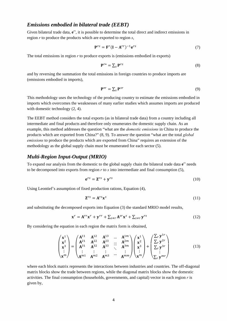
Emissions embodied in bilateral trade (EEBT) Given bilateral trade data, ers, it is possible to determine the total direct and indirect emissions in region r to produce the products which are exported to region s,

(7)

The total emissions in region r to produce exports is (emissions embodied in exports)

• ∑ (8)

and by reversing the summation the total emissions in foreign countries to produce imports are (emissions embodied in imports),

• ∑ (9)

This methodology uses the technology of the producing country to estimate the emissions embodied in imports which overcomes the weaknesses of many earlier studies which assumes imports are produced with domestic technology (2, 4).

The EEBT method considers the total exports (as in bilateral trade data) from a country including all intermediate and final products and therefore only enumerates the domestic supply chain. As an example, this method addresses the question “what are the domestic emissions in China to produce the products which are exported from China?” (8, 9). To answer the question “what are the total global emissions to produce the products which are exported from China” requires an extension of the methodology as the global supply chain must be enumerated for each sector (5).

Multi-Region Input-Output (MRIO) To expand our analysis from the domestic to the global supply chain the bilateral trade data ers needs to be decomposed into exports from region r to s into intermediate and final consumption (5),

(10)

Using Leontief’s assumption of fixed production rations, Equation (4),

(11)

and substituting the decomposed exports into Equation (3) the standard MRIO model results,

∑ ∑ (12)

By considering the equation in each region the matrix form is obtained,

⋮ ⋮ ⋮ ⋮

………⋱… ⋮ ⋮

∑∑∑⋮

∑

(13)

where each block matrix represents the interactions between industries and countries. The off-diagonal matrix blocks show the trade between regions, while the diagonal matrix blocks show the domestic activities. The final consumption (households, governments, and capital) vector in each region r is given by,

5  

⋮ (14)

where yrr is the domestic final consumption of region r. The MRIO model endogenously calculates not only domestic output, but also the output in all other regions resulting from international trade in intermediate products. In single region IOA the matrix elements represents sectors, while in MRIO the block matrices represent regions with each region composed of many sectors. In general, each region can have a different number of sectors, thus the diagonal matrices are always square while the off-diagonal matrices can be rectangular.

TerminologyThe IO literature generally refers to the “emissions embodied in exports/imports”, but a clarification is need on what is meant by “embodied”. The emissions embodied in exports/imports can be defined as the emissions that occur in the production of an exported/imported product. The emissions are not actually a physical part of the product, but rather, are emitted in the production of the product. Following this definition, the carbon in fossil-fuel exports is assumed to be emitted where and when the fuel is oxidized. Thus, the emissions to extract and process the fossil-fuel are allocated to the country of extraction (and processing if it occurs in a separate country) while the emissions to oxidize the fossil-fuel are allocated to the country that oxidizes the fossil-fuel. This is a standard approach in emission inventories.

DifferencesbetweentheEEBTandMRIOmethodsBoth the EEBT and MRIO methods produce the same global emissions, but the allocation between countries is different depending on the structure and level of trade in intermediate products (5). The two methods answer a different type of research question. If the main interest is bilateral trade relationships then the EEBT method is arguably more suitable (10). The EEBT method considers domestic supply chains only and answer questions such as “how much of China’s emissions are from the production of exported goods and services”? For studies at the sub-national level or comparisons of final consumption between countries the MRIO method is arguably more relevant (11). The MRIO method enumerates global supply chains and thus only considers imports to final consumers with trade in intermediate consumption calculated endogenously. The MRIO method answers questions like, “what are the global emissions from household consumption in the USA?” or “what are the global emissions to produce a car in Germany compared to Japan?” Neither method is right nor wrong as they are different ways to attribute emissions from the production of traded products to countries.

The traded emissions allocated to a country will vary depending on whether the MRIO or EEBT method is used (5, 12). Though, it is difficult to determine which will be higher or lower without performing an analysis. The EEBT method includes only the domestic supply chain, while the MRIO includes global supply chains implying that for a given sector the emission intensity will always be greater in the MRIO method. To avoid double counting, however, the MRIO method applies the global emission intensity to final consumption only, while the EEBT method applies the domestic emission intensity to total consumption (intermediate and final consumption). As a consequence, the EEBT method correlates directly with bilateral trade statistics (in proportion to the domestic emission intensity). The MRIO method, correlates directly with final consumption (in proportion to the global emission intensity). The choice of MRIO or EEBT depends on whether the analyst is interested in consumption or bilateral trade. The two methods can be mapped together, via Equation (10), but this is

6  

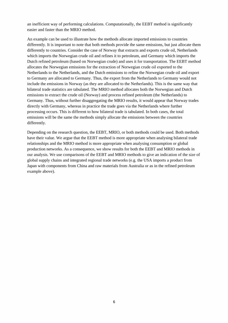
an inefficient way of performing calculations. Computationally, the EEBT method is significantly easier and faster than the MRIO method.

An example can be used to illustrate how the methods allocate imported emissions to countries differently. It is important to note that both methods provide the same emissions, but just allocate them differently to countries. Consider the case of Norway that extracts and exports crude oil, Netherlands which imports the Norwegian crude oil and refines it to petroleum, and Germany which imports the Dutch refined petroleum (based on Norwegian crude) and uses it for transportation. The EEBT method allocates the Norwegian emissions for the extraction of Norwegian crude oil exported to the Netherlands to the Netherlands, and the Dutch emissions to refine the Norwegian crude oil and export to Germany are allocated to Germany. Thus, the export from the Netherlands to Germany would not include the emissions in Norway (as they are allocated to the Netherlands). This is the same way that bilateral trade statistics are tabulated. The MRIO method allocates both the Norwegian and Dutch emissions to extract the crude oil (Norway) and process refined petroleum (the Netherlands) to Germany. Thus, without further disaggregating the MRIO results, it would appear that Norway trades directly with Germany, whereas in practice the trade goes via the Netherlands where further processing occurs. This is different to how bilateral trade is tabulated. In both cases, the total emissions will be the same the methods simply allocate the emissions between the countries differently.

Depending on the research question, the EEBT, MRIO, or both methods could be used. Both methods have their value. We argue that the EEBT method is more appropriate when analysing bilateral trade relationships and the MRIO method is more appropriate when analysing consumption or global production networks. As a consequence, we show results for both the EEBT and MRIO methods in our analysis. We use comparisons of the EEBT and MRIO methods to give an indication of the size of global supply chains and integrated regional trade networks (e.g. the USA imports a product from Japan with components from China and raw materials from Australia or as in the refined petroleum example above).

7  

Estimates of exported and imported emissions 1990-2008 We can only perform the detailed analysis using the EEBT and MRIO methods for the years 1997, 2001, and 2004 due to data availability. However, it is desirable to do the analysis for a longer time period to assess trends in emissions. In our case, we want to analyse emissions since the base year of the Kyoto Protocol in 1990. One option is to construct a detailed EEBT and MRIO database on an annual basis. The development of such a database is a time-consuming exercise and would ultimately mean that the most recent results have a time-lag of several years. As an example, the GTAP database is only available in intervals of 3-5 years and the 2004 data was released in 2008. Several projects are now underway to construct consistent time-series of MRIO tables, but they have not yet reached completion. To avoid the time-lags and construction of an annual global database we develop a method to approximate the EEBT method with the components of the Gross Domestic Product (GDP). We use the EEBT method as a proxy as it is more comparable with the GDP data for this type of analysis. Our method estimates the emissions embodied exports (and imports) on an annual basis using national emission estimates, expenditure components of the GDP, and structural data from GTAP for 1997, 2001, 2004.

GDP is the sum of final consumption expenditures yr (households, government and gross capital formation), exports er, and less imports mr,

(15)

where the same definitions are used as earlier ∑ , ∑ and ∑ . The imports also sum to the use of imported products in the economy as shown in Equation (3). From this relation it is possible to estimate the emissions embodied in exports using the share of exports in GDP as a proxy (13). This estimate is often inaccurate as the supply chain is not included (14, 15) (e.g., aluminum production uses electricity as an input) and final consumption expenditures are a poor representation of economic output (e.g., final consumers only use a small share of the electricity relative to industry). These weaknesses are overcome using the more detailed IOA as described above. Our objective is, therefore, to modify the GDP data to match the results from a one-sector IOA.

We use the GDP data to construct a one-sector IOT analogous to the EEBT method described earlier. The output, as defined in Equation (1), for a one-sector GDP model is given by

(16)

where ∑ include both domestic and imported products. Note that xr and Zr are not available in GDP statistics, but we estimate them below. The direct emission intensity is given by Equation (5) for a one-sector economy,

(17)

Assuming that the intermediate consumption by industry, Zr, is available in GDP statistics, then the Leontief inverse is given by

∑ (18)

Thus, the indirect emission intensity is

∑ (19)

8  

Unfortunately, intermediate consumption of imported products is not available in GDP statistics, but we do have estimates for 1997, 2001, and 2004 from the EEBT method using the GTAP database. We can estimate the imports to industry as a share of total imports, ∑ , where ω is obtained from GTAP. The indirect emission intensity can then be expressed using GDP data only,

(20)

A weakness of using a one-sector GDP approach is that all sectors in the economy have the same emission intensity. It is common that the emission intensity for exports is quite different to the emission intensity for domestically produced and consumed products. We estimate the emission intensity for exports and domestic production using the detailed EEBT results for 1997, 2001, and 2004 from GTAP. We effectively convert the GDP data into a two-sector economy: domestic consumption and exports. As in the EEBT method, imports are produced in another country and are thus considered as an export from the producing country. The emissions in each region for the production of domestic consumption and exports can then be calculated as,

• (21)

1 (22)

where the scaling factor, σ, is the emission intensity of exports relative to the total emission intensity as obtained from the EEBT method for the years 1997, 2001, and 2004.

The method as developed so far gives a top down estimate of the emissions from the production domestic consumption and exports. Results are more policy relevant if the aggregated emissions are further distributed over regions and sectors. In the context of this paper, we are primarily interested in the relocation of production between consuming and producing regions, and thus we want sector detail for the trade flows. One approach to this is to generalise the method to have emission intensities at the

sector detail together with the different final consumption categories (that is, generalize to both sectors and final consumptions). Another approach is to use bilateral trade statistics with annual detail to fill in the missing years. This is the option we have opted for here as it captures the latest developments in international trade flows.

Distributing 1990-2008 estimates over consuming sectors and regions (TSTRD) We use time-series of trade (TSTRD) data and sector emission intensities to distribute the estimated emissions embodied in exports to regions and sectors. This does not change the total amount of exported emissions, Pr(e), in any given year, it only allocates it to sectors and regions. We first apply the detailed emission intensities in 1997, 2001, and 2004 to the annual bilateral trade statistics,

(23)

and secondly normalize the result to match with exported emissions in each year,

•

∑ (24)

The renormalization is necessary to adjust for inflation and inconsistency between the annual bilateral trade statistics and the emission intensities in the base-years 1997, 2001, and 2004. This final expression gives an annual time-series of exported and imported emissions by sector that is consistent

9  

with the EEBT method. For the base-years 1997, 2001, and 2004 the EEBT and TSTRD data should match, but differences arise since the GTAP and UN GDP statistics are different (discussed below).

Our method is based on improving the GDP data using the EEBT method in 1997, 2001, and 2004. We use the 1997 data as a proxy for the GDP data from 1990 to 1998, the 2001 data as a proxy from 1999 to 2002, and the 2004 data as a proxy from 2003 to 2008. To test the robustness of the TSTRD method we compared the results with three proxies with using only two proxies (of which there are three possible combinations). Figure S1 shows the results of this comparison at the Annex B level of detail due to its relevance for the findings in the paper. We also did comparisons for individual countries and found similar results. Our proxies are relatively robust, and the use of three proxies gives a more conservative estimate of the net emission transfer between Annex B and non-Annex B countries. There are two key reasons for the robustness of our results. First, the method is based around the GDP data and the share of exports with the proxies only used to improve the estimate. The GDP and trade data are the same independent of the proxy. Second, our proxies adjust for structural differences and it is known that economic structure changes slowly in comparison to economic volumes (16). This comparison gives us additional confidence of the robustness of our results, however, we perform more detailed comparisons below.

 

Figure S1: A comparison of the TSTRD method using all three proxies (1997, 2001, and 2004) and removing one proxy at a time.

10  

Data sources A variety of data sources are used and in many situations we did some adjustments to make different data sets consistent.

Economic and trade database for the EEBT and MRIO methods (1997, 2001, 2004) The economic data for the EEBT and MRIO methods is based on the Global Trade Analysis Project (GTAP) database (17). We use three versions all with 57 sectors in each region but with 66 regions for the year 1997 (GTAP version 5), 87 regions for 2001 (version 6), and 113 regions for 2004 (version 7). We disaggregate all years to 113 regions for consistent and detailed comparisons. Detailed documentation of the GTAP databases can be found via www.gtap.agecon.purdue.edu. The GTAP database is converted to a MRIO model as in our previous work (10-12). The sectors and regions are shown in Supporting Information Dataset (sheets 1 and 2).

Emissions database for the EEBT and MRIO methods (1997, 2001, 2004) The CO2 emissions are primarily based on GTAP data using the IPCC Tier 1 approach (17), but supplemented with additional sources to cover more accurate data, cement emissions, and flaring (18). Comparisons of the GTAP CO2 data and other national data sources show variations for several reasons (10). First, the system boundary for the energy statistics differs from the economic data (5, 19). Second, the GTAP performs various manipulations on energy data for consistency with other data. Third, there is a known error in the petroleum refineries sector causing an overestimation (17). Finally, region specific emission factors and fuel contents are not used. When national specific emissions data allocated to economic activities were available we overwrote the GTAP data (Australia (20), China (21), Japan (22), USA (23), and EU countries (24)). By comparing the refinery sector emissions in the GTAP data and the national sources we scaled down the refinery emissions in the remainder of the GTAP database. To allow comparisons across datasets we linearly scaled the modified GTAP emissions in each region to match the CDIAC emissions (18).

Database for emissions data (1990-2008) We used the annual fossil-fuel, cement, and gas flaring emissions from 1990 to 2008 from the Carbon Dioxide Information Analysis Center (18) (CDIAC, http://cdiac.ornl.gov). The CDIAC dataset is based energy statistics reported to the United Nations Statistic Division (UNSD) and cement emissions are based on U.S. Department of Interior's Geological Survey. It is not possible to use the officially reported UNFCCC territorial emission statistics as only a limited number of countries have a full time-series from 1990-2008. As a consequence, our territorial emission estimates vary from officially reported statistics. The detailed sector emission estimates for GTAP in 1997, 2001, and 2004 (previous section) also differ in total to the CDIAC estimates due to methodological differences. We scaled the modified GTAP emission statistics to match CDIAC estimates to make the TSTRD method consistent with the EEBT and MRIO estimates. This gives a consistent time series from 1990-2008 covering all methods.

The CDIAC emission estimates only include emissions on nationally administered territory and consequently do not included international transportation in national totals (18) consistent with IPCC definitions (25). For economic analysis, the air and sea traffic in international territory should be allocated to the country where the operator of the vessel is resident (5, 19), corresponding to the user of the bunker fuel. While emission estimates of bunker fuel sales allocated to selling country are available, the necessary data on bunker fuel use allocated to the operator of the vessel are rarely

11  

reported (26). The GTAP emission estimates have a poor representation of bunker fuel emissions (10) and the country level CDIAC emission estimates do not cover bunker fuels. Thus, as in most other studies of this nature, the emissions of international air and sea travel are unreliable though small in magnitude for most countries.

Database for GDP data (1990-2008) The GDP data was obtained from the United Nations Statistic Division (UNSD) National Accounts Main Aggregates Database (http://unstats.un.org/unsd/snaama/Introduction.asp). This database includes time-series of GDP data from 1990 to 2008 measured in current prices with national currencies, current prices in USD, constant prices in national currencies, and constant prices in USD 1990. Since we do annual calculations, our method only requires the more reliable current price data in national currencies which has the additional advantage of not being manipulated using exchange rates or inflation data. Comparisons of the share of exports in GDP showed variations between the constant price and current price data. However, since the constant price data are manipulations of the current price data and have a base year of 1990 we did not feel they were realistic. For example, using 1990 prices for the countries of the former Soviet Union will propagate through the analysis for all years. Likewise, due to rapid changes in the Chinese economy, it is unlikely 1990 prices reflect what happened in 2008. For these reasons we avoided a method requiring constant price data and gave preference to developing a method based on the more reliable current price data.

Database for trade data (1990-2008) The GDP statistics for exports are distributed bilaterally using the GTAP variable TSTRD from version 7. This dataset runs from 1992 to 2006 and has been balanced and adjusted for re-exports (17). It covers bi-lateral trade data between 113 regions and 57 sectors. We extend the data set to 1990 and 2008 by assuming that the bilateral trade shares were the same as in 1992 and 2006 respectively (this only affects the distribution of trade and not the total trade). Since TSTRD only includes manufactured products, we distributed services using the trade shares in the GTAP years 1997, 2001, and 2004.

Currency conversions Since the TSTRD method uses GDP in national currencies, there is no need for currency conversion or inflation adjustments as we did not link the GDP data from different countries though space or time.

The GTAP database combines data from a variety of years to construct a database for the year 1997, 2001, and 2004. GTAP uses market exchange rates (MERs) in the construction of the database (17). The share of exports in GDP may change if purchasing power parity (PPP) is used instead of MERs. In particular, currency conversion based on PPP would reduce the income gaps between countries in the dataset. However, our approach is consistent with dealing with trade flows which are valued in MERs and not consumption levels which are more comparable using PPPs.

Harmonization of datasets The GDP and CDIAC emissions data are both derived from UNSD sources. Despite this, the two datasets do have a slightly different country nomenclature and coverage related to availability of data and changes in country names and boundaries. We reallocated the data to the UN standard country codes (http://unstats.un.org/unsd/methods/m49/m49.htm) for better consistency.

The GTAP and CDIAC national emission totals differ due to different input data and methodology. To allow the estimated exported and imported emissions using the EEBT, MRIO, and GDP methods to be comparable we scaled the GTAP emissions data to match the CDIAC data in 1997, 2001, and 2004.

12  

The GTAP GDP and the UN GDP data differ. GTAP uses GDP statistics for households, government, and capital but replaces exports and imports using bilateral trade statistics in addition to other manipulations (17). It is not possible to modify the GTAP GDP data to match the UN GDP data without a complete rebuild of the GTAP database and GTAP GDP estimates only cover 1997, 2001, and 2004. Even though the GDP estimates vary between the two methods, an analysis of the results shows that the variations are generally small. The differences between the TSTRD method and the EEBT method for the years 1997, 2001, and 2004 are due to the different GDP databases.

13  

Uncertainty in the EEBT and MRIO methods Several authors have discussed the uncertainties in environmentally-extended IOA (27-30). Many types of uncertainties exist, though are usually difficult to quantify due to lack of underlying uncertainty for the IOT. Much of the previous work in the field might thus be better labelled sensitivity analysis rather than uncertainty analysis because often the error and correlation structures have been assumed with insufficient prior information on the uncertainty in underlying input-output data (29, 31). Uncertainty enters into our results in two keys ways: 1) the uncertainty of the input data and 2) errors in the reallocation from producers to consumers. We discuss these two types of uncertainties separately.

Data uncertainty The datasets used in this study ultimately come from many different statistical offices. Particularly for the GTAP database, further internal manipulations are required to harmonize the various data sources and balance the resulting database (17). Uncertainty is, therefore, found in numerous parts of the database. We use this data in the models described above to re-allocate the emissions from producing sectors and regions to consuming sectors and regions.

Despite large potential uncertainties, there is not a strong tradition of performing uncertainty analysis in IOA due to the relative lack of information on uncertainty distributions (27). Often IOTs are created by central statistical agencies within governments and the underlying survey data are not or only partially public. To circumvent the lack of data, analysts often assume uncertainty distributions by assuming that small values have larger uncertainties compared to large values (30). Consistent with this is that studies have found that small values have a minor affect on the results (32). Some studies have employed Monte-Carlo analysis to estimate uncertainties (27, 28, 30, 33). These studies generally find that errors tend to cancel due to the summation and multiplication of many numbers. Thus, despite high uncertainty in individual data points, the overall result may still have relatively low uncertainty. Analysts often resort to qualitative measures of uncertainty (11, 34) and this is often appropriate for a large dataset where the accuracy of an individual data point may be less important than the accuracy of the resulting calculation (35). Thus, more effective would be comparisons between different studies.

Model uncertainty Additional uncertainties arise due to the structure of the IO model. Leontief assumed that the inputs are proportional to outputs (1). This means that irrespective of the size of the purchase, the supply chain will be identical. When dealing with average sector outputs and historic attribution, this linearity should have little impact on the results. As purchases get smaller relative to sector output, it is no longer reliable that the purchase represents the average commodity in a sector and this assumption becomes more problematic. Since we consider aggregated and large flows, this model assumption has only a small effect on the results.

Additional uncertainties arise in the case of MRIOA as linkages need to be made between countries (6, 27). Many of these errors are related to data uncertainty and amplify the uncertainties mentioned earlier. One model related choice is the construction of the MRIOT given bilateral trade statistics. We proportionally distribute the bilateral trade data across sectors and regions according to input structures (5, 11) which is consistent with the GTAP database and hence requires no rebalancing of the MRIOT (17). This assumption means that, for example, the industry use of steel imports into Germany is the same independent of where the steel originated. In practice, one sector may use more steel from one country, while another sector may use more steel from another country.

14  

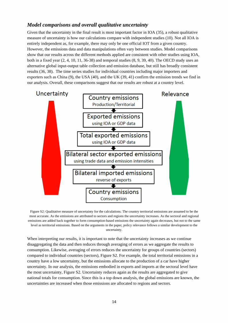
Model comparisons and overall qualitative uncertainty Given that the uncertainty in the final result is most important factor in IOA (35), a robust qualitative measure of uncertainty is how our calculations compare with independent studies (10). Not all IOA is entirely independent as, for example, there may only be one official IOT from a given country. However, the emissions data and data manipulations often vary between studies. Model comparisons show that our results across the different methods applied are consistent with other studies using IOA, both in a fixed year (2, 4, 10, 11, 36-38) and temporal studies (8, 9, 39, 40). The OECD study uses an alternative global input-output table collection and emission database, but still has broadly consistent results (36, 38). The time series studies for individual countries including major importers and exporters such as China (9), the USA (40), and the UK (39, 41) confirm the emission trends we find in our analysis. Overall, these comparisons suggest that our results are robust at a country level.

 

Figure S2: Qualitative measure of uncertainty for the calculations. The country territorial emissions are assumed to be the most accurate. As the emissions are attributed to sectors and regions the uncertainty increases. As the sectoral and regional

emissions are added back together to form consumption-based emissions the uncertainty again decreases, but not to the same level as territorial emissions. Based on the arguments in the paper, policy relevance follows a similar development to the

uncertainty.

When interpreting our results, it is important to note that the uncertainty increases as we continue disaggregating the data and then reduces through averaging of errors as we aggregate the results to consumption. Likewise, averaging of errors reduces the uncertainty for groups of countries (sectors) compared to individual countries (sectors), Figure S2. For example, the total territorial emissions in a country have a low uncertainty, but the emissions allocate to the production of a car have higher uncertainty. In our analysis, the emissions embodied in exports and imports at the sectoral level have the most uncertainty, Figure S2. Uncertainty reduces again as the results are aggregated to give national totals for consumption. Since this is a top down analysis, the global emissions are known, the uncertainties are increased when those emissions are allocated to regions and sectors.

15  

Uncertainty in the TSTRD method The TSTRD method has more uncertainty then the EEBT and MRIO methods. The TRTRD is based on adjusting GDP, bilateral trade, and emissions statistics using the EEBT method. In principle, the EEBT and TSTRD method should agree in 1997, 2001, and 2004, however due to differences in the GDP data in the UN database and GTAP database differences persist primarily since GTAP uses trade statistics in GDP estimates and not reported GDP estimates. The TSTRD method also uses the EEBT data in 1997 to adjust the years 1990-1999, 2001 to adjust 2000-2002, and 2004 to adjust 2003-2008. As one moves further from the adjustment years, uncertainty will increase. Above in Figure S1, we show that our method is relatively robust to changes in the proxy data. This is expected since we 1) base the TSTRD method on the GDP data and 2) use the EEBT proxy data to improve the estimates based on the GDP data. We use a two-step method in constructing the TSTRD estimates by first constructing the total exported emissions and second by allocating the exports to regions and sectors. Thus, the aggregated values are more certain then the disaggregated data. We test the robustness of the TSTRD method by comparing with the EEBT and MRIO methods.

16  

Comparison of the TSTRD, EEBT and MRIO methods

Regional and country results The methods produce a dataset of emissions allocated to either producing or consuming sectors for 113 regions and 57 sectors). Of the 113 regions, 95 individual countries are represented with the remaining countries allocated to aggregated regions based on geo-political similarities due to lack of data (e.g., “Rest of Oceania” is Oceania less Australia and New Zealand). We do not present results for the aggregated “Rest of ...” regions due to poor data quality, though emissions in these countries do contribute to globally traded emissions. As discussed, the global totals are the most certain quantities in the model and the estimates for a given sector-region combination are most uncertain, particularly in small and under developed countries with poor data.

 

Figure S3: The temporal development of the Kyoto Carbon Cycle emissions compared to the EEBT and MRIO methods. The TSTRD estimate is based on the EEBT method and close agreement is expected, with differences primarily due to different GDP data in the UN and GTAP statistics. The differences between the MRIO and EEBT methods are due to regional supply

chains and are discussed in more detail later.

The paper is focused on the allocation of emissions between Annex B and non-Annex B emissions and these are the most certain of our regional results. The major findings of our paper are built on these more certain results. The results give annual emissions in each region to produce domestic consumption and exports. However, in the paper we only consider the allocation to exported products due to their relevance for the Kyoto Protocol. Figure S3 and Supporting Information Dataset (sheet 3) show the temporal development of export related emissions for Annex B and non-Annex B countries in the components of the Kyoto Carbon Cycle. Figure S3 and Supporting Information Dataset (sheet 4) also show the EEBT and MRIO results for 1997, 2001, and 2004. If the GTAP and the UN GDP statistics were identical (see above) then the EEBT and TSTRD methods would be identical in 1997,

17  

2001, and 2004. The difference in the EEBT and MRIO methods are not due to data, but different methodologies. The EEBT method truncates the supply chain at the country border, while the MRIO method consider the global supply chain (5). The EEBT method considers domestic supply chains and total trade between regions, while the MRIO method considers global supply chains and trade in final products with intermediate products treated endogenously. The reason for the underlying differences is discussed below.

Figures S4 and S5 show the regional breakdown of the exports and imports separately. Figure 5 in the main article is the difference of these two figures. Exports from the USA and Europe have grown slowly from 1990-2008 and there has been a slight drop in the other aggregated Annex B countries due to the collapse of the Former Soviet Union. For the aggregated regions, such as Europe, a large share of the trade is between European countries. This cancels with imports in the trade balance, Figure 5. Exports have grown rapidly in most non-Annex B countries with China showing remarkable growth in the last 10 years. A large share of the growth of exports in non-Annex B countries is to other non-Annex B countries, a part of which is ultimately consumed in Annex B countries (see below). The development of imports over time, Figures S5, is different to exports. All countries have had rapid growth in imports from China. Europe had a small drop in imports from the Former Soviet Union in the early 1990’s due to economic collapse which makes European imports look rather stable from 1990-2008 despite strong growth due to China in the last ten years. Most non-Annex B countries have had strong growth in imports and together with strong growth in exports highlights integrated trade networks for components in non-Annex B countries (see below).

Uncertainty increases as the results become increasingly disaggregated, but the method is still stable for key countries and sectors. The Supporting Information Dataset (sheets 5, 6, and 7) shows that the method works well across the 95 individual countries represented in the database. At the country level, uncertainty is larger and variations are noticeable. There is a difference between the TSTRD and the EEBT methods due to variations in GDP across the UN and GTAP datasets and greater fluctuations in the data. The differences are more noticeable as the data values become smaller (that is, smaller countries). This is consistent with IO studies that show greater certainly for larger values. The small and uncertain values tend to cancel at the global level and have a small effect on total results due to their small relative size (see regional comparisons above). The EEBT method is more reliable then the TSTRD method. The differences between the EEBT and MRIO methods are discussed below.

18  

 

Figure S4: Exports by key region using the TSTRD method. Colours represent the destination of the exports.

 

Figure S5: Imports by key region using the TSTRD method. Colours represent the region producing the imports.

19  

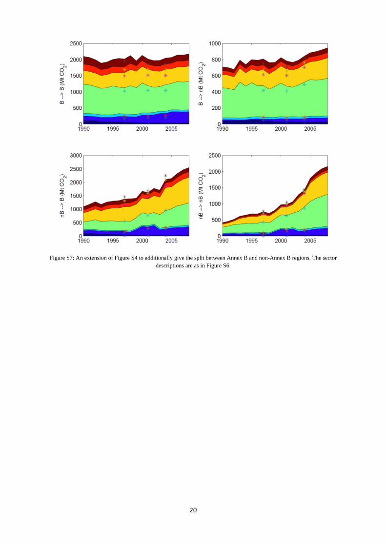
Sector results Figures S6-S7 and the Supporting Information Dataset (sheet 8) show the global, Annex B, and non-Annex B results for seven aggregated sectors. The sectors are aggregated both to reduce uncertainty and enable clear presentation. The totals match the totals in Figure S3, but distributed by sector. Globally, Figure S6, energy-intensive manufacturing (such as metals production, pulp and paper, chemicals, etc) is the most important sector followed by non-energy intensive manufacturing. The mining, transport, and service sectors are the most uncertain (17) in the sector analysis. Figure S7 and the Supporting Information Dataset (sheet 8) show the sector split for Annex B and non-Annex B countries. Figure 5 in the main article is the difference of the Annex B and non-Annex B flows. The emission transfers between Annex B countries have been stable over time despite some growth in emissions due to mining. There has been a slight growth in exports from Annex B to non-Annex B countries due to manufacturing. In contrast there has been rapid growth in exports from non-Annex B countries with most of the growth in manufacturing. Energy intensive manufacturing current takes the biggest share for non-Annex B countries, but growth is fastest in non-energy intensive manufacturing, particularly between non-Annex B countries. This again highlights the importance of regional trade-networks in non-Annex B countries (see below).

 

Figure S6: Total emissions embodied in exports allocated to sector of consumption using the TSTRD method. Each sector includes the domestic supply chain required to produce the product. EEBT method shown with stars.

20  

 

Figure S7: An extension of Figure S4 to additionally give the split between Annex B and non-Annex B regions. The sector descriptions are as in Figure S6.

21  

Additional results and figures

Regional trade-networks: Comparison of the MRIO and EEBT methods The MRIO and EEBT methods are based on the same data, thus differences are due only to the methodology. As described above, the MRIO and EEBT methods allocate emissions to countries in a different way depending on the level of imports which are further processed and then later exported (5) (as distinct from re-exports). The EEBT method truncates the supply chain at national borders and consequently focuses on total exports and imports (10), while the MRIO method considers global supply chains and focuses on final consumption with industry consumption determined endogenously (11). Both methods are correct, they just have a different method of allocation (5).

In combination the EEBT and MRIO methods enable better understanding of integrated global supply chains. Consistent in all the results is that for Annex B and many developed countries, the MRIO estimates of consumption are higher than the EEBT estimates. In the case of Annex B countries, this means that there is trade in unfinished goods and services between non-Annex B countries before the product is ultimately consumed in an Annex B country. For example, Vietnam may export some textiles to China, who exports wearing apparel to the USA or Brazil may export some meat to Mexico who processes the meat and exports to Germany.

Figure S3 and the Supporting Information Dataset (sheet 4) show the difference between the methods.

Focusing on the difference between the EEBT and MRIO methods for Annex-B countries in 1997, 2001, and 2004 provides an indication of the extent of the trade between non-Annex B countries is ultimately to meet Annex B consumption (Figure 2). We find that the MRIO method increases the net emission transfer from non-Annex B to Annex B countries compared to the EEBT method by 47 Mt CO2 in 1997 (8%), by 171 Mt CO2 in 2001 (17%) and by 278 Mt CO2 in 2004 (19%). These results highlight the growing importance of regional trade clusters in unfinished goods and services amongst non-Annex B countries.

Focusing on the difference between the TSTRD and MRIO methods for Annex-B countries in 1997, 2001, and 2004 provides an indication of the extent to which our time-series estimates are conservative (Figure 2). We find that the MRIO method increases the net emission transfer from non-Annex B to Annex B countries compared to the TSTRD method by 102 Mt CO2 in 1997 (18%), by 309 Mt CO2 in 2001 (37%) and by 443 Mt CO2 in 2004 (35%). These results show that, compared to the MRIO method, the TSTRD method underestimates the transfers of emissions between Annex B and non-Annex B countries.

The importance of separating exports and imports The analysis throughout the paper has considered the balance of emissions embodied in trade (42) (BEET), or net emission transfers. Some have argued that an analysis of the trade balance can be misleading as it is natural to imply that a net import of embodied emissions is bad and a net export is good (10). In reality, some countries may always be net importers or exporters (19). For example, Japan is a small country with few natural resources and it may in the long-term import raw materials and export processed products. It may also be desirable to have countries with clean energy systems as net exporters of pollution and countries with dirty energy systems as net importers (19). For example, Norway and Iceland could specialize in the export of electricity-intensive aluminium using their hydropower resources.

22  

Since Annex B countries are to take the lead according to the Kyoto Protocol and Annex B countries can reduce their obligations by increasing imports at the expense of domestic production, arguably imports into Annex B countries from non-Annex B countries may be more important than net transfers as we discussed in the main article. As shown in Table 1, the second fastest growing component of the Kyoto Carbon Cycle is the flow between non-Annex B and Annex B countries, growing much faster than the reverse flow. In addition, a share of the fastest growing component of trade between non-Annex B countries is to meet consumption in Annex B countries (as discussed above). If our analysis is based only on the gross flow from non-Annex B to Annex B countries then the degree to which Annex B countries reduce emission via international trade increases.

Top trade flows The Supporting Information Dataset (sheets 9, 10, and 11) shows the top 30 bilateral trade linkages for country and region linkages, sector and country, and sector between bilateral trade linkages. We only show the average flows from 1990-2008 using the TSTRD method. Linkages with the USA are important, particularly with neighbouring countries. The flow between China and Hong Kong could be unrealistically large reflecting Hong Kong’s role as an entrepôt, though GTAP does make adjustments for this (17). European countries appear lower down the list, though if the EU is aggregated together, then it becomes comparable to the USA. The dominant sectors are often in non-energy intensive products as shown in the main article. This reflects that there are large flows of non-energy intensive products, in addition to the fact that including the supply chain adjusts for energy intensive products that are inputs into non-energy intensive products. The bilateral trade flows by sector provide more detail. Overall, flows between big countries or countries with similar geographic locations are important, in addition to the coverage of non-energy intensive manufacturing due to the inclusion of the supply chain (10).

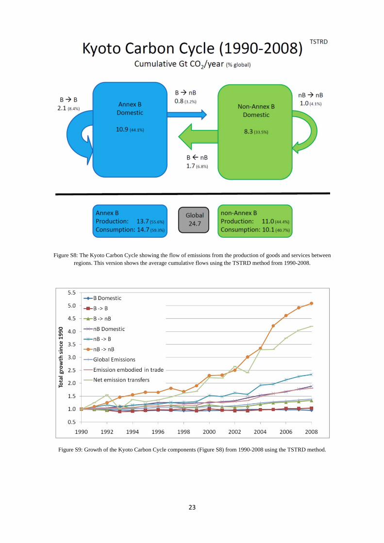
Additional figures for the changes in the Kyoto Carbon Cycle The Kyoto Carbon Cycle (KCC) components can be represented graphically as in Figure S8 showing the rough proportion of aggregated transfers. Figure S8 shows the cumulative proportions in the KCC, while Figure S9 shows the growth of the various components of the KCC. The most rapid growing component, trade between non-Annex B countries, was the least important component in 1990, but now is the equal second most important trade component. Both the trade from non-Annex B to Annex B countries and between non-Annex B countries are growing faster than global emissions. Total global trade is growing at the same rate as non-Annex B domestic emission. Surprisingly, the net emission transfers (B2nB-nB2B) is growing considerably faster than all components except for trade between non-Annex B countries.

23  

 

Figure S8: The Kyoto Carbon Cycle showing the flow of emissions from the production of goods and services between regions. This version shows the average cumulative flows using the TSTRD method from 1990-2008.

 

Figure S9: Growth of the Kyoto Carbon Cycle components (Figure S8) from 1990-2008 using the TSTRD method.

24  

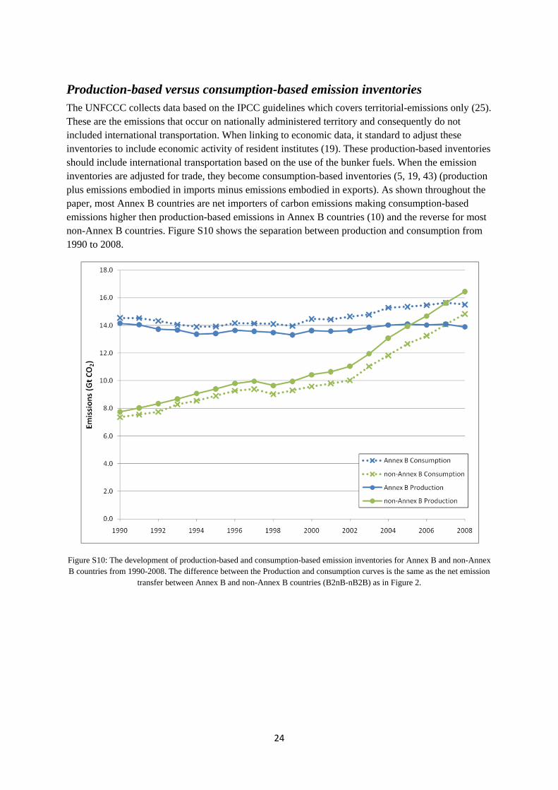
Production-based versus consumption-based emission inventories The UNFCCC collects data based on the IPCC guidelines which covers territorial-emissions only (25). These are the emissions that occur on nationally administered territory and consequently do not included international transportation. When linking to economic data, it standard to adjust these inventories to include economic activity of resident institutes (19). These production-based inventories should include international transportation based on the use of the bunker fuels. When the emission inventories are adjusted for trade, they become consumption-based inventories (5, 19, 43) (production plus emissions embodied in imports minus emissions embodied in exports). As shown throughout the paper, most Annex B countries are net importers of carbon emissions making consumption-based emissions higher then production-based emissions in Annex B countries (10) and the reverse for most non-Annex B countries. Figure S10 shows the separation between production and consumption from 1990 to 2008.

 

Figure S10: The development of production-based and consumption-based emission inventories for Annex B and non-Annex B countries from 1990-2008. The difference between the Production and consumption curves is the same as the net emission

transfer between Annex B and non-Annex B countries (B2nB-nB2B) as in Figure 2.

25  

For individual countries, a shift from production-based to consumption-based emissions changes the ranking of countries, Figure S11. From a production-based perspective China is the world’s largest emitter of CO2 emissions, while the USA is second. The positions are swapped from a consumption-based perspective. Similarly, Japan and the Russian Federation swap positions when shifting from a production- to consumption-based system. The Supporting Information Dataset (sheets 5, 6, and 7) show the emission inventories for production, consumption, and the trade balance for the 95 individual countries in the dataset.

Figure S11: The Top 5 emitters from a consumption-based perspective in 2008 plotted as production-based emissions (left) and as consumption-based emissions (right).

26  

Supporting Information Dataset An attached EXCEL spreadsheet shows the final results from our calculations. The following data is presented: 

Sheet  Name  Description 

1  GTAP_Regions  A list of the 113 GTAP countries and regions 

2  GTAP_Sectors  A list of the 57 GTAP sectors 

3  TSTRD_Overview  An overview of the main TSTRD results, 1990‐2008 

4  TSTRD‐EEBT‐MRIO  A comparison of the TSTRD, EEBT, MRIO methods for 1997, 2001, and 2004 

5  TSTRD_Territorial  The detailed territorial emissions used for all methods 

6  TSTRD_Consumption  The detailed consumption‐based inventory using the TSTRD method 

7  TSTRD_Transfers  The emission transfers for all countries using the TSTRD method 

8  TSTRD_Sectors  The results for the seven aggregated sectors 

9  Top_Regions  The top 30 trade flows between regions 

10  Top_Sectors  The top 30 trade flows by sector 

11  Top_Bilateral  The top 30 bilateral trade flows by sector  

27  

References 1.  Leontief W (1970) Environmental repercussions and the economic structure: An input‐output 

approach. The Review of Economics and Statistics 52(3):262‐271. 2.  Wiedmann T (2009) A review of recent multi‐region input‐output models used for 

consumption‐based emissions and resource accounting. Ecological Economics 69:211‐222. 3.  Wiedmann T (2009) Carbon Footprint and Input‐Output Analysis ‐ An Introduction. Economic 

Systems Research 21:175‐186. 4.  Wiedmann T, Lenzen M, Turner K, & Barrett J (2007) Examining the Global Environmental 

Impact of Regional Consumption Activities ‐ Part 2: Review of input‐output models for the assessment of environmental impacts embodied in trade. Ecological Economics 61:15‐26. 

5.  Peters GP (2008) From Production‐Based to Consumption‐Based National Emission Inventories. Ecological Economics 65:13‐23. 

6.  Peters GP & Hertwich EG (2009) The Application of Multi‐Regional Input‐Output Analysis to Industrial Ecology: Evaluating trans‐boundary environmental impacts. Handbook of Input‐Output Economics in Industrial Ecology, ed Suh S (Springer, Dordrecht). 

7.  United Nations (1999) Handbook of input‐output table compilation and analysis. Studies in Methods Series F, No 74. Handbook of National Accounting (United Nations). 

8.  Guan D, Peters GP, Weber CL, & Hubacek K (2009) Journey to the world top emitter: An analysis of the driving forces of China's recent CO2 emissions surge. Geophysical Research Letters 36:L04709. 

9.  Weber CL, Peters GP, Guan D, & Hubacek K (2008) The Contribution of Chinese Exports to Climate Change. Energy Policy 36:3572‐3577. 

10.  Peters GP & Hertwich EG (2008) CO2 Embodied in International Trade with Implications for Global Climate Policy. Environmental Science and Technology 42:1401‐1407. 

11.  Hertwich EG & Peters GP (2009) Carbon Footprint of Nations: A Global, Trade‐Linked Analysis. Environmental Science and Technology 43:6414‐6420. 

12.  Peters GP, Andrew R, & Lennox J (2011) Constructing a multi‐regional input‐output table using the GTAP database. Economic Systems Research Accepted. 

13.  Wang T & Watson J (2008) China's carbon emissions and international trade: implications for post‐2012 policy. Climate Policy 8:577‐587. 

14.  Huang YA, Lenzen M, Weber CL, Murray J, & Matthews HS (2009) The role of input‐output analysis for the screening of carbon footprints. Economic Systems Research 21:217‐242. 

15.  Matthews HS, Hendrickson CT, & Weber CL (2008) The importance of carbon footprint estimation boundaries. Environmental Science and Technology 42:5839‐5842. 

16.  Hoekstra R & van der Bergh JCJM (2002) Structural decomposition analysis of physical flows in the economy. Environmental and Resource Economics 23:357‐378. 

17.  Narayanan B & Walmsley TL (2008) Global Trade, Assistance, and Production: The GTAP 7 Data Base (Center for Global Trade Analysis, Purdue University). 

18.  Boden TA, Marland G, & Andres RJ (2009) Global, Regional, and National Fossil‐Fuel  CO2 Emissions in Trends.  (Carbon Dioxide Information Analysis Center, Oak Ridge National Laboratory, U.S. Department of Energy, Oak Ridge, Tenn., U.S.A.). 

19.  Peters GP & Hertwich EG (2008) Post‐Kyoto Greenhouse Gas Inventories: Production versus Consumption. Climatic Change 86:51‐66. 

20.  ABS (2001) Energy and Greenhouse Gas Emissions Accounts, Australia 1992‐93 to 1997‐98.  (Australian Bureau of Statistics). 

21.  Peters GP, Weber CL, & Liu J (2006) Construction of Chinese Energy and Emissions Inventory.  (Norwegian University of Science and Technology). 

22.  Nansai K, Moriguchi Y, & Tohmo S (2003) Compilation and application of Japanese inventories for energy consumption and air pollutant emissions using input‐output tables. Environmental Science and Technology 37(9):2005‐‐2015. 

28  

23.  Cicas G, Matthews HS, & Hendrickson C (2006) The 1997 benchmark version of the economic input‐output life‐cycle assessment (EIO‐LCA) model.  (Green Design Institute, Carnegie Mellon University). 

24.  Eurostat (2009) Statistical Office of the European Communities (Online database). 25.  IPCC (2006) IPCC Guidelines for National Greenhouse Gas Inventories, Prepared by the 

National Greenhouse Gas Inventories Programme (IGES, Japan). 26.  Peters GP, et al. (2009) Trade, Transport, and Sinks Extend the Carbon Dioxide Responsibility 

of Countries. Climatic Change 97:379‐388. 27.  Lenzen M (2001) Errors in Conventional and Input‐Output‐based Life‐Cycle Inventories. 

Journal of Industrial Ecology 4:127‐148. 28.  Bullard CW & Sebald AV (1988) Monte Carlo Sensitivity Analysis of Input‐Output Models. The 

Review of Economics and Statistics 70:708‐712. 29.  Williams ED, Weber CL, & Hawkins TR (2009) Hybrid Framework for Managing Uncertainty in 

Life Cycle Inventories. Journal of Industrial Ecology 13:928‐944. 30.  Lenzen M, Wood R, & Wiedmann T (2010) Uncertainty analysis for Multi‐Region Input‐

Output Models ‐ a case study of the UK's carbon footprint. Economic Systems Research 22:43‐63. 

31.  Morgan MG & Henrion M (1990) Uncertainty: A guide to dealing with uncertainty in quantitative risk and policy analysis (Cambridge University Press). 

32.  Oil and Gas Producers (2009) Environmental performance in teh E&P industry ‐ 2008 data.  (International Association of Oil & Gas Producers, Report No: 429). 

33.  Yamakawa A & Peters GP (2009) Using time‐series to measure uncertainty in Environmental Input‐Output Analysis. Economic Systems Research 21:337‐362. 

34.  UNECE (2005) Protocol to the 1979 convention on Long‐Range Transboundary Air Pollution to abate acidification, eutrophication and ground‐level ozone.  (United Nations Economic Commissino for Europe). 

35.  Russian Federation (2010) National Inventory Submissions 2009.  (UNFCCC). 36.  Nakano S, et al. (2009) The measurement of CO2 embodiments in international trade: 

Evidence from the harmonized input‐output and bilateral trade database.  (Organisation for Economic Co‐operation and Development (OECD)). 

37.  Davis SJ & Caldeira K (2010) Consumption‐based Accounting of CO2 Emissions. Proceedings of the National Academy of Sciences 107:5687‐5692. 

38.  Ahmad N & Wyckoff A (2003) Carbon dioxide emissions embodied in international trade of goods.  (Organisation for Economic Co‐operation and Development (OECD)). 

39.  Wiedmann T, et al. (2010) A Carbon Footprint Time‐Series of the UK ‐ Results from a Multi‐Region Input‐Output Model. Economic Systems Research 22:19‐42. 

40.  Weber CL & Matthews HS (2007) Embodied Environmental Emissions in U.S. International Trade, 1997‐2004. Environmental Science and Technology 41:4875‐4881. 

41.  Baiocchi G & Minx JC (2010) Understanding changes in the UK's CO2 emissions ‐ A global perspective. Environmental Science and Technology 44:1177‐1184. 

42.  Muradian R, O'Connor M, & Martinez‐Alier J (2002) Embodied pollution in trade: Estimating the 'environmental load displacement' of industrialised countries. Ecological Economics 41:51‐67. 

43.  Munksgaard J & Pedersen KA (2001) CO2 accounts for open economies: Producer or consumer responsibility? Energy Policy 29:327‐334.