surge nozzle nde specimen mechanical stress … nozzle nde specimen ... 3.6 details of the welding...

PNNL-20549

Prepared for the U.S. Nuclear Regulatory Commission under a Related Services Agreement with the U.S. Department of Energy Contract DE-AC05-76RL01830

Surge Nozzle NDE Specimen Mechanical Stress Improvement Analysis NRC JCN N6319 LF Fredette July 2011

DISCLAIMER This report was prepared as an account of work sponsored by an agency of the United States Government. Neither the United States Government nor any agency thereof, nor Battelle Memorial Institute, nor any of their employees, makes any warranty, express or implied, or assumes any legal liability or responsibility for the accuracy, completeness, or usefulness of any information, apparatus, product, or process disclosed, or represents that its use would not infringe privately owned rights. Reference herein to any specific commercial product, process, or service by trade name, trademark, manufacturer, or otherwise does not necessarily constitute or imply its endorsement, recommendation, or favoring by the United States Government or any agency thereof, or Battelle Memorial Institute. The views and opinions of authors expressed herein do not necessarily state or reflect those of the United States Government or any agency thereof. PACIFIC NORTHWEST NATIONAL LABORATORY operated by BATTELLE for the UNITED STATES DEPARTMENT OF ENERGY under Contract DE-AC05-76RL01830 Printed in the United States of America Available to DOE and DOE contractors from the Office of Scientific and Technical Information,

P.O. Box 62, Oak Ridge, TN 37831-0062; ph: (865) 576-8401 fax: (865) 576-5728

email: [email protected] Available to the public from the National Technical Information Service, U.S. Department of Commerce, 5285 Port Royal Rd., Springfield, VA 22161

ph: (800) 553-6847 fax: (703) 605-6900

email: [email protected] online ordering: http://www.ntis.gov/ordering.htm

This document was printed on recycled paper.

(9/2003)

PNNL-20549

Surge Nozzle NDE Specimen Mechanical Stress Improvement Analysis NRC JCN N6319 LF Fredette(a) July 2011 Prepared for U.S. Nuclear Regulatory Commission under a Related Services Agreement with the U.S. Department of Energy Contract DE-AC05-76RL01830 Pacific Northwest National Laboratory Richland, Washington 99352 _________________________ (a) Battelle Columbus Laboratory; MT Anderson, PNNL Project Manager

iii

Summary

The purpose of this project was to perform a finite element analysis of a pressurized water reactor pressurizer surge nozzle mock-up to predict both the weld residual stresses created in its construction and the final stress state after the application of the Mechanical Stress Improvement Process (MSIP). Strain gages were applied to the inner diameter of the mock-up to record strain changes during the MSIP. These strain readings were used in an attempt to calculate the final stress state of the mock-up as well.

The presentation of the data shows the difficulty in calculating the final stress state based on strain gage measurements in a structure that has experienced yielding stress cycles and has built in residual stresses be they from welding or a yield inducing process like the MSIP. A comparison of the axial and hoop stress values calculated from the strain gage data using three different methods were compared to the finite element analysis predictions. These results show the differences in calculated stresses found when using different assumptions about the initial stress state of the mock-up.

The strain gage measurements indicate that both the axial and hoop stresses in the area of the Alloy 82/182 weld are made compressive by the MSIP process with each of the calculation methods examined.

v

Acronyms and Abbreviations

BWR boiling water reactors DMW dissimilar metal weld EPRI Electric Power Research Institute FEA finite element analysis IGSCC intergranular stress corrosion cracking MSIP Mechanical Stress Improvement Process ORNL Oak Ridge National Laboratory PWR pressurized water reactor

vii

Contents

Summary ...................................................................................................................................................... iii Acronyms and Abbreviations ....................................................................................................................... v 1.0 Introduction ....................................................................................................................................... 1.1 2.0 Discussion of Mechanical Stress Improvement Process.................................................................... 2.1 3.0 Technical Approach of Finite Element Modeling ............................................................................. 3.1

3.1 Pressurizer Surge Nozzle Geometry.......................................................................................... 3.1 3.2 Material Data ............................................................................................................................. 3.2 3.3 Weld Residual Stress Modeling Details .................................................................................... 3.6

4.0 Results from both Finite Element Analysis and Strain Gage Measurements .................................... 4.1 4.1 Strain Gage Instrumentation ...................................................................................................... 4.4 4.2 Conversion of Strain Gage Readings to Stress Values .............................................................. 4.9

4.2.1 Conversion of Strain Gage Readings to Stress Values – Method 1. Disregarding Prior Yielding ............................................................................................................... 4.10

4.2.2 Conversion of Strain Gage Readings to Stress Values – Method 2. Calculating Yielding Stress with MSIP Applied and then Relaxation after MSIP load is Removed from Strain Data Ignoring Weld Residual Stresses ...................................... 4.14

4.2.3 Conversion of Strain Gage Readings to Stress Values – Method 3. Using FEA Predicted Stress with Weld Residual Stress and MSIP Applied and then Calculating Relaxation after MSIP load is Removed from Strain Gage Data. ............. 4.17

5.0 Conclusion ......................................................................................................................................... 5.1 6.0 References ......................................................................................................................................... 6.1

viii

Figures

2.1 Mechanical Stress Improvement Process ......................................................................................... 2.2 3.1 Pressurizer Surge Nozzle Mock-Up Geometry Used in Analysis .................................................... 3.1 3.2 Temperature Dependent True Stress-Strain Curves of Alloy 182 Tested by Oak Ridge

National Laboratories ....................................................................................................................... 3.4 3.3 Temperature Dependent True Stress-Strain Curves of A508 Class 2 Carbon Steel ........................ 3.4 3.4 Temperature Dependent True Stress-Strain Curves of Type 316 Stainless Steel ............................ 3.5 3.5 Surge Nozzle Geometry, Materials, and Weld Layout .................................................................... 3.7 3.6 Details of the Welding Residual Stress Thermal Modeling ............................................................. 3.8 3.7 Surge Nozzle MSIP Application ...................................................................................................... 3.8 4.1 Surge Nozzle Axial Stress ................................................................................................................ 4.1 4.2 Surge Nozzle Mock-Up Axial Stresses along the Inner Diameter ................................................... 4.2 4.3 Surge Nozzle Inner Diameter Hoop Stress Path .............................................................................. 4.3 4.4 Surge Nozzle Inner Diameter Hoop Stresses ................................................................................... 4.3 4.5 Strain Gage Clock Positions ............................................................................................................ 4.4 4.6 Strain Gage Axial Positions ............................................................................................................. 4.5 4.7 Strain Gage Installation .................................................................................................................... 4.5 4.8 MSIP Hydraulic Pressure vs. Axial Strain Gage Readings .............................................................. 4.6 4.9 Post MSIP Axial Strain Gage Readings Plotted against FEA Predictions ....................................... 4.7 4.10 Post MSIP Hoop Strain Gage Readings Plotted against FEA Predictions ....................................... 4.8 4.11 Bi-Linear Stress Strain Curve for 300 Series Stainless Steel ......................................................... 4.10 4.12 Method 1 – Strain to Stress Conversion ......................................................................................... 4.11 4.13 Method 1 Axial Stress Calculations vs. FEA Predictions .............................................................. 4.12 4.14 Method 1 Hoop Stress Calculations vs. FEA Predictions .............................................................. 4.13 4.15 Method 2 – Strain to Stress Conversion ......................................................................................... 4.14 4.16 Method 2 Axial Stress Calculations vs. FEA Predictions .............................................................. 4.15 4.17 Method 2 Hoop Stress Calculations vs. FEA Predictions .............................................................. 4.16 4.18 Method 3 – Strain to Stress Conversion ......................................................................................... 4.17 4.19 Method 3 Axial Stress Calculations vs. FEA Predictions .............................................................. 4.18 4.20 Method 3 Hoop Stress Calculations vs. FEA Predictions .............................................................. 4.19 5.1 Axial Stress – Comparison of Calculation Methods ........................................................................ 5.2 5.2 Hoop Stress – Comparison of Calculation Methods ........................................................................ 5.3

ix

Tables

3.1 Material Properties for Alloy 182 Weld Material ............................................................................ 3.2 3.2 Temperature Dependent Material Properties for A508 Class 2 Carbon Steel ................................. 3.3 3.3 Temperature Dependent Material Properties for Type 316 Stainless Steel ..................................... 3.3 3.4 Temperature Dependent Creep Constants for all the Materials ....................................................... 3.6 4.1 Axial Strain Gage Readings During and After MSIP ...................................................................... 4.7 4.2 Strain Gage Readings During and After MSIP ................................................................................ 4.8 4.3 Method 1 Calculation of Stress from Final Strain State................................................................. 4.13 4.4 Method 2 Calculation of Stress at Final Strain State ..................................................................... 4.16 4.5 Method 3 Calculation of Stress at Final Strain State ..................................................................... 4.19 5.1 Raw Strain Data ............................................................................................................................... 5.4

1.1

1.0 Introduction

The purpose of this project was to perform a finite element analysis of a pressurized water reactor pressurizer surge nozzle mock-up to both predict the weld residual stresses created in its construction and the final stress state after the application of the Mechanical Stress Improvement Process (MSIP). Strain gages were applied to the inner diameter of the mock-up to record strain changes during the MSIP. These strain readings were used in an attempt to calculate the final stress state of the mock-up.

2.1

2.0 Discussion of Mechanical Stress Improvement Process

The MSIP has been used for many years to mitigate intergranular stress corrosion cracking (IGSCC) found in boiling water reactors (BWRs) which have austenitic stainless steel piping and welds. The MSIP was developed and first patented in 1986 (O'Donnell and Porowski 1986; Porowski et al. 1987) by O’Donnell and Associates Inc. Currently the patent is held by NuVision Engineering.

The MSIP tool applies a quasi-radial mechanical loading around the pipe circumference and is positioned to one side of the weld to be treated. The distance from the weld centerline to the MSIP tool is in the range of 25 to 100 mm (1 to 4 inches) depending on the geometry. The tool hydraulically squeezes the pipe and is displacement-controlled by the use of shims. The loading plastically deforms the pipe in compression under the tool which creates beneficial compressive stresses on the inside diameter of the adjacent welded region.

The MSIP effect has been extensively documented in two Electric Power Research Institute (EPRI) reports. In the earliest report, dating from 1987, large diameter (28-inch diameter) pipes were welded and tested (Smith et al. 1987). The scope of the testing was designed to determine the MSIP’s change of weld stress patterns, the effect on pre-existing defects, and the effect on the detectability of pre-existing defects after the process. The later report, from 1993, documents experiments on smaller diameter (12-inch diameter) nozzle geometries (Phillips et al. 1993). Both studies found similar results. Smith et al. (1987) measured as-welded, inner diameter, axial tensile stresses in the 275 MPa to 414 MPa (40 ksi to 60 ksi) range, which were uniformly converted to compressive stresses in the −69 MPa to −241 MPa (−10 ksi to −35 ksi) range after application of the MSIP.

Figure 2.1 shows the schematic of the application of the MSIP on a surge nozzle geometry. The original patent (O'Donnell and Porowski 1986) for the process states that the permanent reduction of the diameter of the pipe at the mid-plane of the applied load should be 0.2 to 2.0 percent. In this study a baseline value of 1% reduction in diameter was used for the analysis and 0.94% was achieved during the test on the mock-up. The patent also states that the distance between the mid-plane of the weld to be treated and the mid-plane of the load application site should be 2 to 12 times the pipe thickness. The edge of the applied MSIP load band should be at least equal to half the wall thickness away from the weld centerline.

The MSIP has been used successfully on over 1,300 welds, including more than 500 nozzle safe end geometries in over 30 BWR units and now in pressurized water reactor (PWR) units as well according to NuVision Engineering the holder of the patent on the MSIP process.

2.2

Figure 2.1. Mechanical Stress Improvement Process

3.1

3.0 Technical Approach of Finite Element Modeling

Two dimensional axi-symmetric finite element models were used to calculate the weld residual stresses in the treated weld. The use of axi-symmetric models allowed for finer mesh refinement and computational efficiency in running the multiple load cases and sensitivity studies that were conducted. The MSIP is not truly axi-symmetric in its application. Three-dimensional models of the MSIP were not evaluated in this study but were used on a similar geometry in a previous study (Fredette et al. 2008; Fredette and Scott 2009). Three dimensional models of the process have shown that even though the MSIP application does not produce a uniform effect around the circumference of the pipe; it is effective over the entire circumference of the treated weld. Strain gage placement at 90o circumferential spacing was used to capture this effect.

Preceding evaluations of the MSIP have been conducted using physical test specimens and axi-symmetric finite element models (Smith et al. 1987; Phillips et al. 1993). The process, as illustrated in Figure 2.1, uses two 180° spacers to squeeze the pipe segment. The spacers are held in a fairly rigid steel structure, and pulled together with hydraulic pistons. The spacers are made to conform to the geometry of the pipe system, a nozzle in this case. The radial gap between the spacer and the pipe segment to be treated is made to further conform to the pipe shape with crushable waffled stainless steel shims. The purpose of the crushable shims is to make the loading more uniformly radial by conforming to surface irregularities on the pipe.

3.1 Pressurizer Surge Nozzle Geometry

Figure 3.1 shows a revolved version of the axi-symmetric pressurizer surge nozzle mock-up geometry with the weld area highlighted. The nozzle is carbon steel; the butter (green in the figure), dissimilar metal weld (maroon in the figure) are made from Alloy 82/182; and the safe end, secondary stainless steel weld (orange in the figure), and pipe are made from 300 series stainless steel material.

Figure 3.1. Pressurizer Surge Nozzle Mock-Up Geometry Used in Analysis

3.2

3.2 Material Data

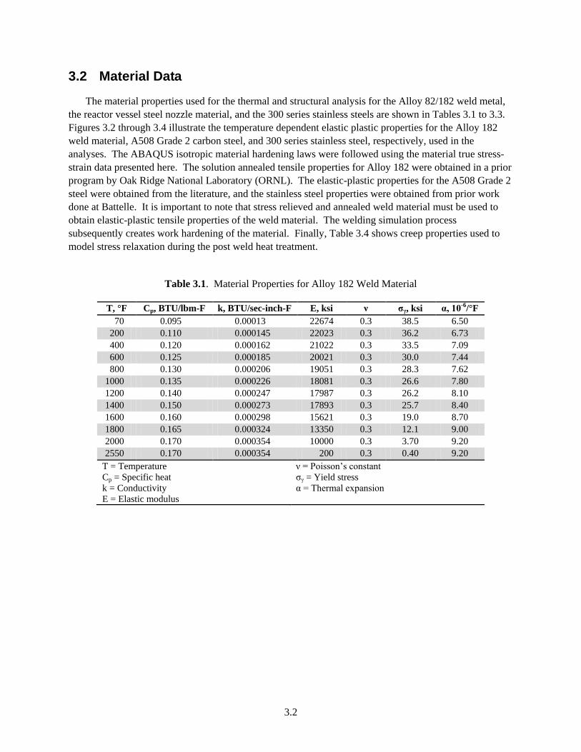
The material properties used for the thermal and structural analysis for the Alloy 82/182 weld metal, the reactor vessel steel nozzle material, and the 300 series stainless steels are shown in Tables 3.1 to 3.3. Figures 3.2 through 3.4 illustrate the temperature dependent elastic plastic properties for the Alloy 182 weld material, A508 Grade 2 carbon steel, and 300 series stainless steel, respectively, used in the analyses. The ABAQUS isotropic material hardening laws were followed using the material true stress-strain data presented here. The solution annealed tensile properties for Alloy 182 were obtained in a prior program by Oak Ridge National Laboratory (ORNL). The elastic-plastic properties for the A508 Grade 2 steel were obtained from the literature, and the stainless steel properties were obtained from prior work done at Battelle. It is important to note that stress relieved and annealed weld material must be used to obtain elastic-plastic tensile properties of the weld material. The welding simulation process subsequently creates work hardening of the material. Finally, Table 3.4 shows creep properties used to model stress relaxation during the post weld heat treatment.

Table 3.1. Material Properties for Alloy 182 Weld Material

T, °F Cp, BTU/lbm-F k, BTU/sec-inch-F E, ksi ν σγ, ksi α, 10-6/°F 70 0.095 0.00013 22674 0.3 38.5 6.50

200 0.110 0.000145 22023 0.3 36.2 6.73 400 0.120 0.000162 21022 0.3 33.5 7.09 600 0.125 0.000185 20021 0.3 30.0 7.44 800 0.130 0.000206 19051 0.3 28.3 7.62

1000 0.135 0.000226 18081 0.3 26.6 7.80 1200 0.140 0.000247 17987 0.3 26.2 8.10 1400 0.150 0.000273 17893 0.3 25.7 8.40 1600 0.160 0.000298 15621 0.3 19.0 8.70 1800 0.165 0.000324 13350 0.3 12.1 9.00 2000 0.170 0.000354 10000 0.3 3.70 9.20 2550 0.170 0.000354 200 0.3 0.40 9.20

T = Temperature Cp = Specific heat k = Conductivity E = Elastic modulus

ν = Poisson’s constant σγ = Yield stress α = Thermal expansion

3.3

Table 3.2. Temperature Dependent Material Properties for A508 Class 2 Carbon Steel

T, °F Cp, BTU/lbm-F T, °F k, BTU/sec-inch-F T, °F E, ksi ν σγ, ksi α, 10-6/°F 70 0.11 32 0.000694 71.6 30784 0.3 54.5 7.67

122 0.116 212 0.00067 600 28807 0.3 43.8 7.67 302 0.124 392 0.000647 1000 25633 0.3 29.5 8.33 392 0.127 572 0.000617 1400 14540 0.3 9.78 8.61 482 0.133 752 0.000571 1800 10243 0.3 2.78 8.89 572 0.137 932 0.000527 2732 203 0.3 0.44 8.89 662 0.143 1112 0.000476 842 0.158 1292 0.000425

1022 0.179 1472 0.000348 1202 0.202 1832 0.000364 1292 0.342 2192 0.000397 1382 0.227 1562 0.215 1832 0.202 2192 0.201

T = Temperature Cp = Specific heat k = Conductivity E = Elastic modulus


Table 3.3. Temperature Dependent Material Properties for Type 316 Stainless Steel

T, °F Cp, BTU/lbm-F T, °F k, BTU/sec-inch-F T, °F E, ksi ν σγ, ksi α, 10-6/°F 74 0.1079 70 0.000173 75 28400 0.3 38.0 8.09

165 0.1132 200 0.000186 300 27500 0.3 30.0 8.77 191 0.1143 400 0.000207 550 25950 0.3 23.4 9.33 400 0.1229 623 0.000231 700 24900 0.3 23.0 9.57 603 0.1291 800 0.000248 900 23500 0.3 22.0 9.84 794 0.132 1011 0.000269 1100 22200 0.3 20.5 10.09

1020 0.136 1195 0.000288 1300 20820 0.3 20.0 10.21 1204 0.1398 1391 0.000308 1500 19100 0.3 17.0 10.43 1410 0.145 1583 0.000327 1652 16900 0.3 14.1 10.60 1595 0.1505 1783 0.000348 1832 14500 0.3 8.46 10.70 1784 0.1556 1996 0.000369 2012 14500 0.3 3.77 10.90 1996 0.1622 2732 203 0.3 0.44 11.20 T = Temperature Cp = Specific heat k = Conductivity E = Elastic modulus


3.4

Figure 3.2. Temperature Dependent True Stress-Strain Curves of Alloy 182 Tested by Oak Ridge

National Laboratories

Figure 3.3. Temperature Dependent True Stress-Strain Curves of A508 Class 2 Carbon Steel

3.5

Figure 3.4. Temperature Dependent True Stress-Strain Curves of Type 316 Stainless Steel

3.6

Table 3.4. Temperature Dependent Creep Constants for all the Materials

A n T, °F MATERIAL: A508 Class2

1.0000E-26 4.0000 70 2.2910E-12 6.0451 1000 3.2670E-07 4.8865 1200 3.2670E-07 4.8865 1200

MATERIAL: S309, S304, S316 1.0000E-26 4.0000 70 9.2650E-25 9.7800 887 4.6900E-24 9.9700 932 1.6410E-21 9.0600 977 3.9710E-19 8.2000 1022 2.7540E-18 8.2000 1067 1.7060E-17 8.2000 1112 1.1700E-16 8.1800 1157 7.2180E-16 8.1600 1202 3.4110E-14 7.4200 1247 1.3300E-12 6.7200 1292 2.0930E-11 6.2500 1337 3.2310E-10 5.7700 1382

MATERIAL: Alloy 182 1.0000E-26 4.0000 70 1.0000E-26 4.0000 990 2.1478E-16 6.1709 1000 4.6025E-15 6.6426 1100 4.6025E-15 6.6426 2500

nA tε = σ where inCreep rate in hr

ε =⋅

A = Material constant σ = Von Mises stress (ksi) n = Material constant t = Time (hr)

3.3 Weld Residual Stress Modeling Details

The welding produced residual stresses were calculated using an axi-symmetric model. The finite element model was subjected to a thermal analysis, which simulated the weld process functions of laying down the molten beads of weld filler metal, introducing heat energy into the weld bead and cooling the weld to an appropriate inter-pass temperature. The thermal analysis calculated the temperatures throughout the finite element model through the welding process. A subsequent stress analysis was performed which used the previously defined temperatures to calculate the elastic-plastic residual stresses and strains in the welded geometry due to the thermal effects of welding. ABAQUS finite element software was used throughout the study. Material properties used in the analyses varied with temperature and made use of the annealing simulation capabilities of the ABAQUS software to model weld bead melting (Dassault Systèmes 2007).

3.7

Figure 3.5 shows the pressurizer surge nozzle mock-up axi-symmetric geometry. This configuration contained a low alloy steel nozzle and a welded Alloy 82/182 buttering on the end. The stainless steel safe end component was welded to the buttered nozzle with Alloy 82/182 weld filler. After the primary Alloy weld was completed, a standard practice is to grind out the root pass and re-weld that area. This process tends to increase the inner diameter axial tension stresses and was modeled in the analysis. In the mock-up, pre-made flaws were welded into the inner diameter of the Alloy 82/182 weld for non-destructive examination purposes and this inner diameter welding would produce a similar tension increasing effect. In close proximity to the Alloy 82/182 weld is another weld fabricated with stainless steel weld filler material which connects the stainless steel safe end to the stainless steel piping.

Figure 3.5. Surge Nozzle Geometry, Materials, and Weld Layout

Figure 3.6 shows the transient thermal analysis steps used to model the thermal portion of the weld residual stress analysis for an example surge nozzle geometry. Between weld passes, the weld was allowed to cool to an inter-pass temperature of 66°C (150°F). The root pass of the Alloy 82/182 weld was ground out and re-welded as a final step in the weld process. This step is not always performed during plant fabrication, but was included here because it increases the interior tension stresses in the weld and is thus conservative. The inner diameter grinding and welding of the flaws into this mock-up provide a similar process that increases inner diameter tensile stresses. It is unclear whether the entire root pass was ground out in the mock-up, but portions of it were removed and re-welded in the final steps of the welding process to implant pre-made flaws to be used in a non-destructive examination test.

3.8

Figure 3.6. Details of the Welding Residual Stress Thermal Modeling (°F)

Figure 3.7 shows the schematic of the axi-symmetric application of the MSIP. The original patent for the process states that the permanent reduction of the diameter of the pipe at the mid-plane of the applied load should be 0.2 to 2.0%. In this study a baseline value of 1% reduction in diameter was used and further evaluated through sensitivity analyses. The patent also states that the distance between the mid-plane of the weld to be treated and the mid-plane of the load application site should be 2 to 12 times the pipe thickness. The edge of the applied MSIP load band should be at least equal to half the wall thickness away from the weld centerline.

Figure 3.7. Surge Nozzle MSIP Application

3.9

The values used for this nozzle comply with the requirements described in the original patent (Porowski et al. 1987) and fall in the typical range of 1% reduction in diameter, two times the wall thickness between midpoints, and one times the wall thickness to the edge of the load application site. When the application location of the MSIP falls over the location of the secondary weld, as is this case, a gap is made in the tool to avoid the crown of the secondary weld as shown in the figure, and included in the tooling used on the mock-up.

4.1

4.0 Results from both Finite Element Analysis and Strain Gage Measurements

The pressurizer surge nozzle weld residual stresses were developed as shown in Figure 3.6. Though described previously in some detail, the process deserves another explanation here. The figure shows the initial welding of the butter layer plus the post weld heat treatment of the buttered nozzle at 593°C (1,100°F) for four hours during which creep properties are allowed to relax the welding residual stresses in the butter layer. The butter layer is then pre-heated to 121°C (250°F), and the dissimilar metal weld is then built up pass-by-pass until the weld is complete as shown in Figure 3.7. This process joins the stainless steel safe end to the carbon steel nozzle. The dissimilar metal weld (DMW) is allowed to cool to approximately 66°C (150°F) between passes and to room temperature after the weld is complete. The root pass is then ground out and re-welded. When the Alloy 82/182 weld is complete and cooled to room temperature, the secondary stainless steel weld is built up and then allowed to cool to room temperature once completed.

Figure 4.1 shows the axial stress contour plot after the Alloy 82/182 welding is complete (top figure), after the stainless steel safe end weld is complete (middle figure), and after the MSIP has been performed (bottom figure). Figure 4.2 shows the axial stress along the inner diameter of the mock-up with the location of the butter, Alloy 82/182 weld, and stainless steel weld indicated by vertical color coded bands in the graph.

Figure 4.1. Surge Nozzle Axial Stress (ksi)

4.2

Figure 4.2. Surge Nozzle Mock-Up Axial Stresses along the Inner Diameter

One can see that the stress was very high in the butter and dissimilar metal weld before the secondary stainless steel weld is made. Once the secondary stainless steel weld is completed, the stresses along the inner diameter are primarily compressive except in the area of the transition between the carbon steel nozzle and the butter. In this area the stresses remain tensile in the range of 40 ksi (276 MPa). After the MSIP is completed, all of the stresses along the inner diameter have been made compressive up to the location of the secondary stainless steel weld.

The PWSCC occurrences are typically found in the dissimilar metal weld at the interface between the pressure vessel steel material and the butter layer, or between the butter and the Alloy 82/182 weld. The weld residual stresses in the stainless steel weld are of less importance.

Figure 4.3 shows the hoop stress contour plots and Figure 4.4 show the inner diameter hoop stress along the length of the dissimilar metal weld area of the surge nozzle. The graph shows that hoop stresses are very high on the inner diameter before the secondary stainless steel weld is made, and are reduced, but remain highly tensile after the stainless steel weld is completed. The stresses remain high in the area of the butter transition to the carbon steel nozzle. The MSIP reduces the hoop stresses in the area of concern to be compressive over the whole length of the dissimilar metal weld area.

4.3

Figure 4.3. Surge Nozzle Inner Diameter Hoop Stress Path (ksi)

Figure 4.4. Surge Nozzle Inner Diameter Hoop Stresses

4.4

4.1 Strain Gage Instrumentation

Figure 4.5 and Figure 4.6 show the clock position and axial position of the strain gages used to instrument the surge nozzle mock-up. The strain gages were placed at 0° and 90° with 0° being the top position in the MSIP process. Five locations were used at each angular position spaced one inch apart spanning the length of the safe end. In each of the locations, a 2-element, 90° biaxial rosette gage was used to measure both axial and hoop direction strains. Previous three-dimensional MSIP modeling has shown that the compressive hoop stress produced during and after the MSIP process so overwhelms the welding residual stresses, that the principal stresses in the area of measurement are in the axial and hoop directions. The gages were Vishay Micro-Measurements 0.032-in. gage, 120-Ohm strain gages. They each used three wires in a quarter bridge arrangement. Their gage factor was 2.06 and they were calibrated for the thermal expansion of steel. The gages were read with a Vishay Strain Indicator P-3500 that was calibrated at the Battelle instrument lab on April 15, 2009, and the next calibration was not due until May 15, 2010, five months after the test was done. Two Vishay Instruments SB-10 switch and balance units were used to wire up the twenty strain gages used in the test. The strain gage locations are numbered #1–#5 with #5 being closer to the Alloy 82/182 weld.

Figure 4.7 shows the strain gage installation at both 0° and 90°. The features on the inside surface of the mockup can be compared with the spacing shown in Figure 4.6.

Figure 4.5. Strain Gage Clock Positions

4.5

Figure 4.6. Strain Gage Axial Positions

Figure 4.7. Strain Gage Installation

Figure 4.8 shows the axial strain gage readings vs. applied hydraulic pressure during the MSIP application. The graph looks like a typical stress strain plot showing yielding. Though strain gages at positions #2 and #3 in the 90° clock position failed at the highest MSIP load, the strain gages appeared to be working normally up to that point. The hoop strain gage results look similar, but all values are negative.

Figure 4.9 and Table 4.1 show the axial strain values plotted against two finite element model curves. The red dashed curve represents the finite element analysis (FEA) predicted axial strain in a case where there were no initial weld residual stresses, and MSIP was applied. The solid darker red curve represents the FEA predicted axial strain in the case in which weld residual stresses were present before the MSIP. The strain gage data matches the predictions reasonably well. The strain gage data shows similar results

4.6

to the FEA predictions and is a near perfect match in some locations. The values start out in compression near the Alloy 82/182 weld, and peak at 1% strain which is the permanent radial deformation caused by the MSIP, and then are reduced to values in the range of 0.5% strain similar to the FEA prediction with no initial weld residual stresses toward the safe end weld. The table shows that the axial strains are all positive except for locations #5 which are all negative. The table also shows that the strain is reduced for all positive cases after the MSIP tool is released, and the strain actually increases when the tool is released for the compressive locations #5.

Figure 4.8. MSIP Hydraulic Pressure vs. Axial Strain Gage Readings

4.7

Figure 4.9. Post MSIP Axial Strain Gage Readings Plotted against FEA Predictions

Table 4.1. Axial Strain Gage Readings During and After MSIP

Gage Position Code Axial Readings with MSIP

Load Applied, in/in Axial Readings after

MSIP, in/in 0° #1 Axial 0.0049 0.0043 0° #2 Axial 0.0066 0.0055 0° #3 Axial 0.0130 0.0101 0° #4 Axial 0.0046 0.0031 0° #5 Axial −0.0001 −0.0003

90° #1 Axial 0.0026 0.0022 90° #2 Axial Failed Failed 90° #3 Axial Failed Failed 90° #4 Axial 0.0058 0.0039 90° #5 Axial −0.0012 −0.0014

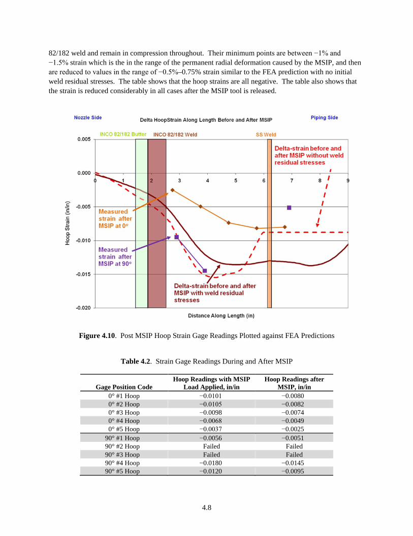
Figure 4.10 and Table 4.2 show the hoop strain values plotted against the same two finite element model curves, but for hoop strain in this case. The red dashed curve represents the FEA predicted hoop strain in a case where there were no initial weld residual stresses, and MSIP was applied. The solid darker red curve represents the FEA predicted hoop strain in the case in which weld residual stresses were present before the MSIP. Again, the strain gage data matches the predictions reasonably well with the 90° location matching better than the 0° location. The values start out in compression near the Alloy

4.8

82/182 weld and remain in compression throughout. Their minimum points are between −1% and −1.5% strain which is the in the range of the permanent radial deformation caused by the MSIP, and then are reduced to values in the range of −0.5%–0.75% strain similar to the FEA prediction with no initial weld residual stresses. The table shows that the hoop strains are all negative. The table also shows that the strain is reduced considerably in all cases after the MSIP tool is released.

Figure 4.10. Post MSIP Hoop Strain Gage Readings Plotted against FEA Predictions

Table 4.2. Strain Gage Readings During and After MSIP

Gage Position Code Hoop Readings with MSIP

Load Applied, in/in Hoop Readings after

MSIP, in/in 0° #1 Hoop −0.0101 −0.0080 0° #2 Hoop −0.0105 −0.0082 0° #3 Hoop −0.0098 −0.0074 0° #4 Hoop −0.0068 −0.0049 0° #5 Hoop −0.0037 −0.0025

90° #1 Hoop −0.0056 −0.0051 90° #2 Hoop Failed Failed 90° #3 Hoop Failed Failed 90° #4 Hoop −0.0180 −0.0145 90° #5 Hoop −0.0120 −0.0095

4.9

4.2 Conversion of Strain Gage Readings to Stress Values

People are generally more comfortable working with stresses than strains, but the conversion of strain to stress values in cases in which there has been yielding, or in the cases of welding, with many yielding cycles, is not easy. Strain gages only give results for ∆-strain from the initial state in which the gages were applied. No valid stress results can be drawn without knowing the original stress state of the mock-up. To illustrate this point calculated stress values will be made with the following assumptions:

1. Using only the post MSIP strain values as other methods such as x-ray diffraction, neutron diffraction, and hole drilling would produce from a final strain state measurement.

2. Using the yielded stress state with the MSIP load applied, and the strain relaxation after the MSIP load was released to predict the final stress state assuming no initial weld residual stresses.

3. Using the FEA prediction for weld residual stress and yielding under the MSIP tool load and then calculating the final stress state by operating on these stress values with the measured strain relaxation (∆-strain between the case with MSIP load applied and released.)

The following bi-linear stress-strain curve was used for the type 316 stainless steel shown in Figure 4.11. A similar curve was used for the FEA analysis. Isotropic strain hardening was assumed with linear stress relaxation following the Young’s Modulus curve upon load release. Strain gage readings were converted to stress using the plane stress equations shown in Eq. (4.1) where stress is denoted by (σ), Young’s Modulus is denoted by (E), strain is denoted by (ε), and Poisson’s Ratio is denoted by (µ). Previous three-dimensional MSIP modeling has shown that the compressive hoop stress produced during and after the MSIP process so overwhelms the welding residual stresses, that the principal stresses in the area of measurement are in the axial and hoop directions.

Axial Hoop

Axial 2

Hoop AxialHoop 2

Plane Stress Equationsμ

E1-μ

μE

1-μ

ε + ε σ =

ε + ε

σ =

(4.1)

4.10

Figure 4.11. Bi-Linear Stress Strain Curve for 300 Series Stainless Steel

4.2.1 Conversion of Strain Gage Readings to Stress Values – Method 1. Disregarding Prior Yielding

The first method of converting strain readings to stress values disregards the prior yielding history of the mock-up and uses only the post MSIP strain values as other methods such as x-ray diffraction, neutron diffraction, and hole drilling would produce from a final strain state measurement. This calculation will produce an incorrect result because the original stress state, and the path through yielding caused by the MSIP tool is not taken into account. Stress is calculated following the bi-linear stress-strain curve shown in Figure 4.12 or the mirror image for compressive strains. The bi-axial stress equations are used considering both axial and hoop stresses and the Poisson’s Ratio effects.

4.11

Figure 4.12. Method 1 – Strain to Stress Conversion

Figure 4.13, Figure 4.14, and Table 4.3 show the stress results from Method 1 vs. the finite element predictions for the case where there is only the stress caused by the MSIP process and no initial weld residual stresses. The axial stress plot, Figure 4.13, shows some agreement between the calculated stress from the strain data and the FEA model predictions. The values are compressive near the Alloy 82/182 weld, and tensile under the location where the MSIP tool is applied. There is a large spacing between the strain gage results at the two clock positions. The hoop stress plot, Figure 4.14, does show agreement between the gage results at each clock positions, but the results show uniform compressive stresses slightly beyond yielding and well below the values that the finite element analysis predicts.

4.12

Figure 4.13. Method 1 Axial Stress Calculations vs. FEA Predictions

4.13

Figure 4.14. Method 1 Hoop Stress Calculations vs. FEA Predictions

Table 4.3. Method 1 Calculation of Stress from Final Strain State

Gage Position Code

Axial Readings after MSIP, in/in

Hoop Readings after MSIP, in/in

Calculated Non-Linear Axial Stress

after MSIP Load, psi

Calculated Non-Linear Hoop Stress

after MSIP Load, psi 0° #1 0.0043 −0.0080 41,623 −43,057 0° #2 0.0055 −0.0082 41,961 −43,007 0° #3 0.0101 −0.0074 43,432 −42,353 0° #4 0.0031 −0.0049 41,531 −42,251 0° #5 −0.0003 −0.0025 −31,158 −41,814

90° #1 0.0022 −0.0051 22,990 −42,379 90° #2 Failed Failed Failed Failed 90° #3 Failed Failed Failed Failed 90° #4 0.0039 −0.0145 −9,628 −45,032 90° #5 −0.0014 −0.0095 −42,286 −44,000

4.14

4.2.2 Conversion of Strain Gage Readings to Stress Values – Method 2. Calculating Yielding Stress with MSIP Applied and then Relaxation after MSIP load is Removed from Strain Data Ignoring Weld Residual Stresses

The second method explored for converting strain readings to stress values uses the yielding strain caused by the MSIP application and then the strain relaxation afterward to predict the final stress state as shown in Figure 4.15. The bi-axial stress equations are used considering both axial and hoop stresses and the Poisson’s Ratio effects. A calculation of the Von Mises stress for each of the strain gage positions shows that they are all well beyond the yield point when the MSIP load is applied. This result should be closer to correct, but still disregards the initial weld residual stresses in the mock-up.


Figure 4.16, Figure 4.17, and Table 4.4 show the stress results from Method 2 vs. the finite element predictions for the case where there is only the stress caused by the MSIP process and no initial weld residual stresses. The axial stress plot, Figure 4.16, shows better agreement between the calculated stress from the strain data and the FEA model predictions. The values are compressive near the Alloy 82/182 weld, and tensile under the location where the MSIP tool is applied. The slope of the curve near the Alloy 82/182 weld better matches that of the FEA prediction, and the values from the two clock positions are closer together. The hoop stress plot, Figure 4.17, now do not show agreement between the clock positions, but the slope of the curve near the Alloy 82/182 weld is similar between them. The 0° location shows better agreement with the FEA prediction with compressive values near the Alloy 82/182 weld.

4.15


4.16


Table 4.4. Method 2 Calculation of Stress at Final Strain State

Gage Position

Code

Calculated Non-Linear Axial Stress with MSIP Load, psi

Calculated Non-Linear Hoop Stress with MSIP Load, psi

Δ-Axial Strain from MSIP Load Applied to Released,

in/in

Calculated Axial Stress

Biaxial Relaxation,

psi

Δ-Hoop Strain from MSIP Load Applied to Released,

in/in

Calculated Hoop Stress

Biaxial Relaxation,

psi

Calculated Axial Stress after MSIP,

psi

Calculated Hoop Stress after MSIP,

psi 0° #1 41,606 −43,650 −0.0006 1,760 0.0021 61,436 43,366 17,786 0° #2 42,089 −43,615 −0.0011 −13,191 0.0024 63,032 28,897 19,417 0° #3 44,072 −42,832 −0.0028 −66,237 0.0024 49,623 −22,165 6,791 0° #4 41,832 −42,674 −0.0016 −31,233 0.0019 43,784 10,599 1,110 0° #5 −36,499 −42,153 −0.0002 5,341 0.0012 35,167 −31,158 −6,986

90° #1 30,597 −42,500 −0.0004 −7,607 0.0005 12,475 22,990 −30,025 90° #2 Failed Failed Failed Failed Failed Failed Failed Failed 90° #3 Failed Failed Failed Failed Failed Failed Failed Failed 90° #4 15,427 −45,941 −0.0019 −25,055 0.0036 94,164 −9,628 42,126 90° #5 −42,458 −44,752 −0.0002 17,793 0.0026 77,907 −24,665 33,155

4.17

4.2.3 Conversion of Strain Gage Readings to Stress Values – Method 3. Using FEA Predicted Stress with Weld Residual Stress and MSIP Applied and then Calculating Relaxation after MSIP load is Removed from Strain Gage Data.

The third method uses the FEA prediction of weld residual stresses and the additional yielding caused by the application of the MSIP load as a starting point. The final stress state is calculated using the strain gage data and the ∆-strain measured between the case with the MSIP load applied, and when it is released. Figure 4.18 graphically shows the concept of the calculation. Stress and strain in steps #1 and #2 are predicted by the finite element model, and the delta strain and stress between steps #2 and #3 are calculated from the strain gage data. This method will give stresses closest to reality because of the inclusion of initial weld residual stresses but depends on the accuracy of the finite element model as a starting point.


Figure 4.19, Figure 4.20, and Table 4.5 show the stress results from Method 3 vs. the finite element predictions for the case where weld residual stresses and the stress caused by the MSIP process are considered. The axial stress plot, Figure 4.19, shows very good agreement between the calculated stress from the strain data and the FEA model predictions. The values are compressive near the Alloy 82/182 weld, and slightly tensile under the location where the MSIP tool is applied. The slope of the curve near the Alloy 82/182 weld matches very well that of the FEA prediction. The values from the two clock positions are fairly close together. The hoop stress plot, Figure 4.20, shows very good agreement between

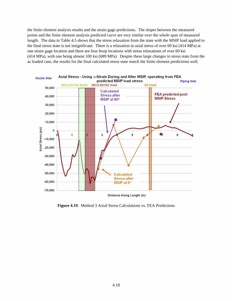
4.18

the finite element analysis results and the strain gage predictions. The slopes between the measured points and the finite element analysis predicted curve are very similar over the whole span of measured length. The data in Table 4.5 shows that the stress relaxation from the state with the MSIP load applied to the final stress state is not insignificant. There is a relaxation in axial stress of over 60 ksi (414 MPa) at one strain gage location and there are four hoop locations with stress relaxations of over 60 ksi (414 MPa), with one being almost 100 ksi (689 MPa). Despite these large changes in stress state from the as loaded case, the results for the final calculated stress state match the finite element predictions well.


4.19


Table 4.5. Method 3 Calculation of Stress at Final Strain State

Gage Position

Code

FEA Axial Stress

with MSIP Load, psi

FEA Hoop Stress with

MSIP Load, psi

Delta-Axial Strain from MSIP Load Applied to Released,

in/in

Calculated Axial Stress

Biaxial Relaxation,

psi

Delta-Hoop Strain from MSIP Load Applied to Released,

in/in

Calculated Hoop Stress

Biaxial Relaxation,

psi

Calculated Axial Stress after MSIP,

psi

Calculated Hoop Stress after MSIP,

psi 0° #1 3,516 −51,024 −0.0006 1,760 0.0021 61,436 5,276 10,412 0° #2 4,921 −55,377 −0.0011 −13,191 0.0024 63,032 −8,270 7,655 0° #3 25,428 −23,102 −0.0028 −66,237 0.0024 49,623 −40,809 26,521 0° #4 37,887 −7,538 −0.0016 −31,233 0.0019 43,784 6,654 36,246 0° #5 −50,258 −86,182 −0.0002 5,341 0.0012 35,167 −44,917 −51,015

90° #1 3,516 −51,024 −0.0004 −7,607 0.0005 12,475 −4,091 −38,549 90° #2 4,921 −55,377 Failed Failed Failed Failed Failed Failed 90° #3 25,428 −23,102 Failed Failed Failed Failed Failed Failed 90° #4 37,887 −7,538 −0.0019 −25,055 0.0036 94,164 12,832 42,510 90° #5 −50,258 −86,182 −0.0002 17,793 0.0026 77,907 −32,465 −8,275

5.1

5.0 Conclusion

This project used finite element analysis of a pressurized water reactor pressurizer surge nozzle mock-up to predict both the weld residual stresses created in its construction and the final stress state after the application of the Mechanical Stress Improvement Process (MSIP). Also, strain gages were applied to the inner diameter of the mock-up to record strain changes during and after the application of the MSIP. These strain readings were used in an attempt to calculate the final stress state of the mock-up as well.

The presentation of the data shows the difficulty in calculating the final stress state based on strain gage data in a structure that has experienced yielding stress cycles and has built in residual stresses be they from welding or a yield inducing process like the MSIP. Figures 5.1 and 5.2 show a comparison of the axial and hoop stress values calculated from the strain gage data using the three different methods discussed previously compared to the finite element analysis predictions. The results calculated for the axial stress at strain gage #3 at the 0o position is suspected of providing a faulty delta-strain measurement between the load cases in which the MSIP was applied and after it was released. The axial stress graph indicates results as solid lines with strain gage #3 data removed for Method #2 and Method #3 in which the delta-strain measurement is used in the calculation of stress. Dashed lines indicate the suspected faulty results provided by strain gage #3. The suspected faulty measurement is only evident after comparison of the stress calculations, and with the knowledge that strain gages #2 and #3 in the 90o position failed before the full MSIP load was applied at a similar strain reading of 1.3-1.4% (see Table 5.1 for raw strain measurements). This only further illustrates the care that must be taken in reviewing strain measurements in such a residual stress field.

In all cases examined, the strain gage measurements indicate that both the axial and hoop stresses in the area of the Alloy 82/182 weld are made compressive by the MSIP process.

5.2

Figure 5.1. Axial Stress – Comparison of Calculation Methods

5.3

Figure 5.2. Hoop Stress – Comparison of Calculation Methods

5.4

Table 5.1. Raw Strain Data

Gage Position

Code

Readings with Gages

Zeroed, in/in

2,000 psi Hydraulic Pressure,

in/in


in/in


in/in


in/in


in/in


in/in


in/in


in/in


in/in

MSIP Load

Applied 20,000 psi,

in/in

Readings after

MSIP, in/in

0° #1 Axial 0.0000 0.0000 0.0001 0.0002 0.0002 0.0004 0.0007 0.0009 0.0015 0.0026 0.0049 0.0043 0° #1 Hoop 0.0000 −0.0002 −0.0004 −0.0007 −0.0011 −0.0015 −0.0022 −0.0029 −0.0041 −0.0062 −0.0101 −0.0080 0° #2 Axial 0.0000 0.0001 0.0002 0.0003 0.0005 0.0008 0.0012 0.0016 0.0024 0.0037 0.0066 0.0055 0° #2 Hoop 0.0000 −0.0002 −0.0005 −0.0009 −0.0012 −0.0018 −0.0025 −0.0032 −0.0044 −0.0066 −0.0105 −0.0082 0° #3 Axial 0.0000 0.0002 0.0004 0.0007 0.0011 0.0016 0.0023 0.0031 0.0045 0.0071 0.0130 0.0101 0° #3 Hoop 0.0000 −0.0003 −0.0006 −0.0010 −0.0013 −0.0018 −0.0025 −0.0032 −0.0043 −0.0062 −0.0098 −0.0074 0° #4 Axial 0.0000 0.0001 0.0003 0.0005 0.0006 0.0009 0.0012 0.0016 0.0021 0.0030 0.0046 0.0031 0° #4 Hoop 0.0000 −0.0003 −0.0005 −0.0008 −0.0011 −0.0015 −0.0020 −0.0025 −0.0033 −0.0045 −0.0068 −0.0049 0° #5 Axial 0.0000 0.0000 0.0001 0.0001 0.0002 0.0002 0.0003 0.0003 0.0003 0.0002 −0.0001 −0.0003 0° #5 Hoop 0.0000 −0.0002 −0.0004 −0.0006 −0.0008 −0.0010 −0.0014 −0.0017 −0.0021 −0.0027 −0.0037 −0.0025 90° #1 Axial 0.0000 0.0000 0.0000 0.0001 0.0001 0.0003 0.0006 0.0010 0.0019 0.0035 0.0026 0.0022 90° #1 Hoop 0.0000 −0.0003 −0.0006 −0.0010 −0.0015 −0.0023 −0.0035 −0.0051 −0.0080 −0.0136 −0.0056 −0.0051 90° #2 Axial 0.0000 0.0002 0.0004 0.0006 0.0009 0.0013 0.0019 0.0026 0.0038 0.0060 Failed Failed 90° #2 Hoop 0.0000 −0.0004 −0.0008 −0.0013 −0.0019 −0.0028 −0.0041 −0.0057 −0.0087 −0.0144 Failed Failed 90° #3 Axial 0.0000 0.0005 0.0011 0.0018 0.0025 0.0036 0.0050 0.0066 0.0093 0.0142 Failed Failed 90° #3 Hoop 0.0000 −0.0005 −0.0009 −0.0016 −0.0022 −0.0031 −0.0044 −0.0060 −0.0086 −0.0138 Failed Failed 90° #4 Axial 0.0000 0.0004 0.0007 0.0009 0.0011 0.0015 0.0020 0.0024 0.0029 0.0037 0.0058 0.0039 90° #4 Hoop 0.0000 −0.0004 −0.0008 −0.0012 −0.0017 −0.0024 −0.0033 −0.0044 −0.0063 −0.0099 −0.0180 −0.0145 90° #5 Axial 0.0000 0.0001 0.0002 0.0003 0.0003 0.0003 0.0002 0.0001 0.0000 −0.0004 −0.0012 −0.0014 90° #5 Hoop 0.0000 −0.0003 −0.0005 −0.0008 −0.0011 −0.0016 −0.0022 −0.0029 −0.0042 −0.0066 −0.0120 −0.0095

6.1

6.0 References

Dassault Systèmes. 2007. "ABAQUS, V6.7-1." Dassault Systèmes, Providence, Rhode Island.

Fredette L and PM Scott. 2009. Evaluation of the Mechanical Stress Improvement Process (MSIP) as a Mitigation Strategy for Primary Water Stress Corrosion Cracking in Pressurized Water Reactors. Battelle Columbus, Columbus, Ohio. U.S. NRC Agencywide Data Access and Management System (ADAMS) Accession Number ML092990646.

Fredette L, PM Scott and FW Brust. 2008. "An Analytical Evaluation of the Efficacy of the Mechanical Stress Improvement Process in Pressurized Water Reactor Primary Cooling Piping." In Proceedings of the ASME 2008 Pressure Vessels and Piping Division Conference. July 27-31, 2008, Chicago, Illinois. American Society of Mechanical Engineers, New York. Paper #PVP2008-61484.

O'Donnell WJ and JS Porowski. 1986. "Mechanical Stress Improvement Process." U.S. Patent 4,612,071.

Phillips MK, SJ Findlan, D Gandy, A Peterson and S Walker. 1993. Evaluation of Repair, Replacement, Mitigation and Examination Approaches for Boiling Water Reactor Nozzle/Safe-End Configurations. Electric Power Research Institute, Palo Alto, California.

Porowski JS, WJ O'Donnell, ML Badlani and EJ Hampton. 1987. "Mechanical Stress Improvement Process." U.S. Patent 4,683,014.

Smith RE, KE Perry and WH Wolf. 1987. An Application of the Mechanical Stress Improvement Process to Large-Bore Piping. EPRI Report Number T305-1, Electric Power Research Institute, Palo Alto, California.

surge nozzle nde specimen mechanical stress … nozzle nde specimen ... 3.6 details of the welding...

Documents