Survey of Implementation and Visualization of

Neural Networks

Nate GaunttUniversity of New MexicoDept. of Computer Science

Email : negaunt@cs.unm.edu

Abstract - Modern Graphics Processing Units (GPUs) are cheap,ubiquitous, and increasing in performance at a rate two to three timesthat of traditional CPU growth. As GPUs evolve in function and be-come ever more programmable each generation, they are increasinglyput to use in various high throughput parallel calculations, such assolving fluid flow equations or simulating plate tectonics. In thispaper, we discuss the recent trend in implementing classical NeuralNetwork architectures on the GPU, allowing in some cases real timeinput processing, and in other cases dramatic speedup of traditionalalgorithms. Also, we discuss a broad survey of techniques developedwithin the last 20 years to analyze the often non-linear dynamics ofneural systems.

1 Introduction

In the early 1940’s and throughout the 50’s, paritally as a result of Ameri-can and British codebreaking activities, the theory of computation became anarea of active research in the scientific community. In a 1943 paper publishedby Warren McCullogh and Walter Pitts [2], a formal system is created thatmathematically describes the behavior of biological neurons and networks ofneurons. Using this system, they show that, with sufficient neurons and properconnections, any computable function can be represented by such a network ofneurons. In 1969, Minsky and Papert [3] explain the serious mathematical lim-itations of a single artificial neuron, including it’s inability to learn the trivialXOR boolean function. This symbolist critique cast doubt on the efficacy ofusing neural networks (NNs) for learning tasks for more than a decade untila revival of the technique in the 1980’s [4], when an efficient method of errorfeedback learning called back-propogation was discovered.

Just as connectionist methodology flourished in the 80’s and early 90’s af-ter efficient error feedback was discovered, modern graphics hardware provides

1

another efficiency revolution, allowing neural networks to be applied easily andcheaply to certain real-time problems and other throughput-sensitive domains.It is only within the last several years that Graphics Processing Units (here-after GPUs) have had the ability to store results efficiently to 32-bit textures(GeForce 8, 2006), have been able to be programmed by high level languagessuch as Cg (2002), or have had the tool support to be used together in robusthigh-performance architectures like CUDA (2006) [5, 7, 8]. There has been muchresearch in the last several years describing advancements in implementation ofneural networks using such parallel hardware, which we will address presently.

2 GPU Economic Advantages

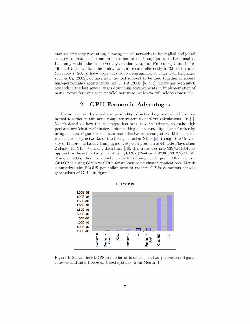
Previously, we discussed the possibility of networking several GPUs con-nected together in the same computer system to perform calculations. In [1],Meuth describes how this technique has been used in industry to make highperformance ’cluster of clusters’, often taking the commodity aspect further byusing clusters of game consoles as cost-effective supercomputers. Little successwas achieved by networks of the first-generation XBox [9], though the Univer-sity of Illinois - Urbana Champaign developed a productive 64 node Playstation2 cluster for $15,000. Using data from [10], this translates into $39/GFLOP, asopposed to the estimated price of using CPUs (Pentium4-3200), $312/GFLOP.Thus, in 2005, there is already an order of magnitude price difference perGFLOP in using GPUs vs CPUs for at least some cluster applications. Meuthsummarizes the FLOPS per dollar ratio of modern CPUs vs various consolegenerations of GPUs in figure 1.

Figure 1: Shows the FLOPS per dollar ratio of the past two generations of gameconsoles and Intel Processor-based systems, from Meuth [1]

2

3 Neural Network Implementations

Neural Network implementations on the GPU have evolved with the chang-ing state of the underlying hardware. One of the earlier implementations isby Bohn [13], who implements Kohonen feature mapping on an SGI worksta-tion. His efficient implementation in OpenGL is possible through acceleratedGL functions glColorMatrix, and glminmax, and various texture blending func-tions. This behavior was possible utilizing expensive SGI workstations; however,the modern trend was to sacrifice accelerated 2D functions for better 3D perfor-mance. Given the minor programmability of hardware at the time, Bohn reliesheavily on OpenGL blending functions, tying such an implementation to vendorsupport of an accelerated high-level API.

In the early 2000’s, much effort was spent investigating increasingly pro-grammable GPUs, and their application to scientific computing [14, 15]. Fastlinear algebra on the GPU requires fast matrix multiply implementations, andthis work led to several neural network GPU implementations utilizing matrixmultipy routines. Rolfes [12] does this, using a blend of DirectX and hand-tunedGPU assembly code. Unlike Bohn, Rolfes relies less on accelerated DirectX calls,but instead relies on fast implementation of certain GPU instructions and hand-tuned assembly code. Rolfes’ implementation is somewhat more portable andless fragile than Bohn’s, but still relies on implementation details, which are con-stantly in flux, in order to achieve good performance. The main contributionof this implementation techinique is to accelerate multi-layer perceptron (MLP)neural networks on commodity graphics hardware. For another matrix-basedcomputation of MLP, see Kyoung-Su’s [?] implementation, used for real-timetext detection in a video stream. Kyoung-Su achieves a 20-fold performanceincrease over CPU implementation.

As the language of high level shader programming became standard andGPU compiler optimization improved, implementors began moving to higherlevel implementations of neural networks. Zhongwen et. al. [11] used Cg toimplement both self organizing map (SOM) and MLP neural networks. Despitethe high level language, some knowledge of GPU instructions is needed to con-struct efficient algorithms. For example, to find the minimum value (or bestmatch) in the SOM, Zhongwen uses a recursive algorithm dividing the activa-tion space into 4 at each step, until only scalar 2x2 matrices are left. This mayseem puzzling without the knowledge that most GPUs have an efficient minfunction that computes the minimum of 2 4-vectors. Zhongwen achieves a 2 to4 fold performance advantage in SOM over the CPU, and 200 fold performanceadvantage over CPU implementation. It is not known what CPU implementa-tion is used, or if it is even optimized, so it is important to carefully considerperformance claims. That said, Zhongwen’s MLP was able to compute an ob-ject tracking function in 46 ms, which they note is theoretically fast enough tobe useful for real-time response. Zhongwen also notes several caveats of highlevel implementations. In one case the same Cg code yielded correct results on

3

the ATI card and incorrect results on the NVidia card, so a code change wasneeded to work around a probable hardware defect. The performance of GPUcode is very sensitive to the number of rendering passes and data transfer to theCPU, which they minimized where possible. Also they note that 32-bit floatingpoint textures were critical to the accuracy of the MLP, a feature that is notfully supported on many graphics cards, and may also suffer from SGI patentrestrictions [6].

Figure 2: SOM training time, CPU vs ATI / NVidia GPU, from Zhongwen [11]

While Cg provides a language low level enough to be portable across graph-ics APIs (such as DirectX and OpenGL), but high enough to avoid hardware-dependant and cumbersome GPU assembly code, it is not the only languageused for writing flexible shader programs. Recently, Davis explores the use ofBrookGPU [17], a stream programming framework designed for use on the GPU.BrookGPU is slightly higher level than Cg, abstracting the details of shader andvertex programs running on the GPU, instead focusing on input streams beingoperated on by special functions called kernels. The compiler enforces limi-tations inside kernel functions to ensure only efficient operations are executedon the GPU. The main benefit, as Davis explains in [4], is portability, as asingle BrookGPU program can be targeted to DirectX or OpenGL. Similarly,BrookGPU allows the programmer to focus on algorithm design, rather thanon handling graphics API calls or decyphering shader language syntax. Daviswas able to quickly implement Hopfield, MLP, and Fuzzy ART neural networks,and compare the BrookGPU to CPU implementations. For MLP and Hopfieldnetworks, ATLAS BLAS optimized linear algebra suite was used in the CPUimplementation, and complete code for both BrookGPU and CPU implementa-tions is given. Davis was able to realize a modest 2 fold performance increaseover CPU for MLP and Hopfield networks; however, the Fuzzy ART implemen-

4

tation was dramatically slower than the CPU. The reason given for this is thatBrookGPU’s stream model doesn’t support certain useful texture memory up-dates, and presumably other low level optimizations, that Cg allows. Similar toZhongwen, Davis finds significant performance differences between NVidia andATI performance for the same code (see figure 3), suggesting that high levelimplementations are sensitive to hardware differences. Another explantion isthat the NVidia and ATI shader program compilers have signficant differencesin optimizing code. In either case, programmer caution is advised.

Figure 3: Calculation time in MLP vs. network layers, from [4]. Red NVidiaand green ATI BrookGPU code are better than CPU as layers increase

Spiking neural networks are often more interesting to neurobiologists thanthe MLP neural network, as they preserve more information about the dynam-ics of neurons and more closely resemble biological neurons. With this fidelitycomes cost, and where MLP neurons are updated on each processor timestep,spiking networks may take up to 100 timesteps to update a neuron. To thisend, several researchers have developed GPU algorithms for simulating thesenetworks more efficiently [18, 19]. In [18], Bernhard uses spiking networks tosolve an image segmentation problem. Neurons are connected locally for ex-itation for regions of similar color, and are connected globally for inhibitionregardless of color. Reading locally from a few number of exitatory neurons inparallel is efficient for fast GPU texture memory, but reading all other neuronsfor global inhibition is not. Bernhard solves this by adding an additional pass

5

where a pixel is written to only if a neuron has fired. Then, using an occlusionquery, he counts the number of pixels written, and this is the same as the globalinhibition for the neuron. Since GPUs accelerate occlusion queries, this resultsin a 5 to 7 times speed increase versus CPU timings. An unrelated benefitof simulating neural networks on the GPU is ease of visulization. Figure 4 isalmost literally successive memory dumps of the GPU algorithm as it executes.

Figure 4: Time series evolution of spiking neurons for image segmentation, from[18]. Areas of similar color are similar activation level

Nageswaran’s approach also models spiking neural networks, though at asignificantly greater level of biological plausibility. In order to do this, he usesCUDA, similar in some ways to BrookGPU in that it abstracts the GPU as amultiprocessor, capable of running lightweight threads simultaneously and ac-cessing shared memory through texture memory. Threads in CUDA can bescheduled in groups by the on-GPU hardware scheduler, such that if a threadin the group stalls reading GPU texture memory, another non-stalled group canrun. Similar to parallel distributed systems literature, complex CUDA algo-rithms have the same kind of problems with synchronization and optimization.Despite this, Nageswaran et. al. were able to simulate 100K neurons with 50Msynaptic connections with a 25 fold speedup over a CPU implementation, over-all being only 1.5 times slower than real-time (ie. one update per timestep). Itis interesting to note that in both spiking network implementations that learn-ing takes place on the GPU, which is rare for GPU neural networks. Part ofwhy it is efficient to do “learning updates” for spiking networks is that insteadof weights being represented by contents of memory addresses, they are repre-sented by firing frequency, implicitely calculated by the simulation itself.

Fuzzy ART is perhaps a middle ground between the minimal analytic modelof MLP networks and the biologically correct spiking networks, and it’s imple-mentation on the GPU derives in part from various clustering algorithms onthe GPU, such as SOM in [11, 13]. Martinez-Zarzuela et. al. implement FuzzyART on the GPU, in two parts, in [20]. The first part is a GPU ART networkoptimized for learning, and another GPU ART network optimized for testing.The learning ART parallelizes at calculating input activations and sorting forthe best category match. The sorting for best category match closely resemblesthe best match reduction Zhongwen uses for SOM, and the updating of ART

6

weights is accomplished by rendering into a sub-region of a texture via scissor-ing. Where training calculates neuron response and best match in parallel for asingle input vector, testing calculates category for several input vectors simul-taneously. Testing calculates the first category for n input vectors, and the firstcategory response for each input vector is stored in parallel to n textures. Thesen textures are fed back into the network, and if the second category responseis greater, it will overwrite the category number. This process continues untilall categories have a chance to respond and compete. Unfortunately, trainingupdates tended to be the performance bottleneck, with the GPU training net-work running 10 to 100 fold slower than a CPU implementation, whereas theGPU testing network had no such bottleneck and ran 25 to 46 fold faster thanthe CPU. The authors note that un-optimized memory transfer from CPU toGPU is a potential source of improvement for the testing network. See [21, 22]for GPU treatment of related non-neural clustering algorithms.

4 Neural Network Visualization

Since the connectionist counter-revolution of the 1980’s, researchers havebeen using neural networks productively for many and varied tasks, such as ap-proximating atmospheric lighting in [23]. Unfortunately, the non-linear natureof even small, feed-forward networks makes them difficult to formally analyze,and may have been the source of the original (erroneous) critique of generalMLP networks by Papert and Minsky. If the result of the neural network isprimarily visual, or if the algorithm performs image or video processing, thevisual debugging or presentation of the neural network can be straightforward,such as in figures 4, 5, or in [23]. If the result of the network is an arbitraryclassification task; however, the visual interpretation is far from obvious.

An earlier work in visual analysis of neural networks is the Hinton diagramin [24]. In figure 6, each black square is a network of neurons responding to theinput, which can be thought of as a query. The response is shown by the size ofthe squares, which when viewed en masse, show which part of a large networkis responding to the input. This is also an early example of semantic zooming,where on one plate, Hinton represents a network with squares corresponding toneuron activation, and on the next plate, he represents a network of networks,with squares corresponding to average network activation.

Another earlier work by Dennis [25] uses principal component analysis (PCA)and canonical discriminant analysis (CDA) to plot the hidden layer activationsof a feed-forward network as it learns a classification task. PCA plots the datapoints along axes which maximize variance and preserve, to some extent, dis-tance between points in the original space and the transformed space. CDArequires points to be labelled by cluster group, and plots the data points alongaxes which cluster points within groups while maximizing distance between

7

Figure 5: Visual debugging: black pixels are ones categorized as containing text,from [16]

Figure 6: Hinton Diagram: squares are memory networks, size is average net-work response to input. Darker rows represent a stored pattern in memory.

8

groups. Unlike PCA, CDA cannot work on unlabelled data, and CDA doesn’tnecessarily preserve distance between points in the original space and the trans-formed space. CDA, in figure 7 gives a more meaningful picture of the hiddenunit state evolution, but requires a priori knowledge about the task, which isprobably unsuitable for networks using unsupervised learning. The historicaldiscussion of automatic techniques like PCA versus guided techniques like CDAis important, as there is a tension in the literature as to (1) what level of apriori knowledge it is appropriate to assume and get unbiased results, and (2)how to differentiate between meaningful clustering and accidental clustering incomplicated statistics involving high dimensional data.

Figure 7: Left: CDA plot of hidden layer Right: PCA plot of hidden layerVisualization of hidden layer weights in MLP as network learns, from [25]

MLPs are by far the most popular network visualized in the literature,Craven collects and summarizes several techniques in [26]. These include aversion of Hinton diagrams modified to show polarity and typically spatiallyorganized to show directional connections, see figure 8.

Figure 8: Modified Hinton diagram: size and color are magnitude and polarityof activation, spatial position is connection geometry, from [26]

9

Wejchert and Tesauro develop another way of visualizing MLP networks in[27]. In figure 9, a bond diagram is displayed, its namesake deriving from weightsbeing displayed as variable length and colored “bonds”, where the visible frac-tion of the length corresponds to the weight magnitude and the color correpondsto the weight polarity. Also, the size of the neurons (white circles) that originatethe bonds corresponds to the magnitude of the bias weight. Craven notes thatthe advantage over Hinton diagrams is that bond diagrams show network topol-ogy in a more obvious way. The disadvantage of this technique, notes Craven,is that it is difficult to compare the magnitude of the bias with the magnitudeof the bonds, as one is represented primarily by area and the other by relativelength.

Figure 9: Bond diagram: The white circles represent neurons, circle size is biasmagnitude, bond length is connection weight, bond color is weight polarity, from[26]

They develop another visualization technique in the same paper, calledtrajectory diagrams reminding one of Charles Josepth Minard’s diagram ofNapoleon’s eastern Europe campaign in [30]. Figure 10 shows such a diagram,where the axes are ranges over two of the input weights to this neuron, and thethickness of the line is proportional to error.

Pratt and Nicodemus develop a tool to display moving hyperplanes in theframe of the input space as the neurons learn, see figure 11 for details. Thoughthey discuss mostly feature spaces of length 2, this method could be applied toarbitrary length input vectors by using PCA or a related statistical technique tofind a meaningful 2D representation. Like CDA, however, animated hyperplanesremain meaningful only when working with labelled classifier data, and so obeythe same limitations of CDA or other high dimensional clustering techniques.

Lang developed a similar technique in the late 80’s to display hyperplaneresponse to input stimulus in [29]. The x and y axis represent the full range oftwo components of an input vector, and the gray level magnitude is the activa-tion, with white and black representing polarity, see figure 12.

10

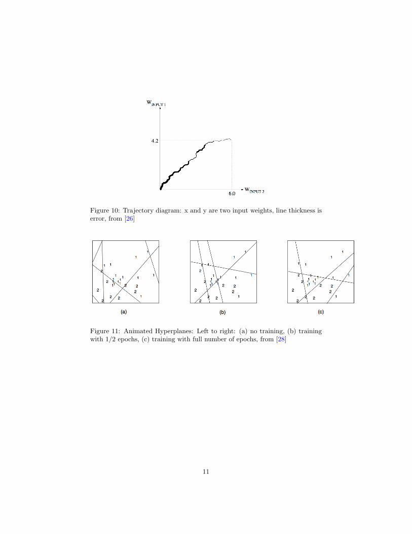
Figure 10: Trajectory diagram: x and y are two input weights, line thickness iserror, from [26]

Figure 11: Animated Hyperplanes: Left to right: (a) no training, (b) trainingwith 1/2 epochs, (c) training with full number of epochs, from [28]

11

Figure 12: Response function plots: x and y are input ranges, gray level isactivation. Left to Right: three hidden unit responses to input, from [26]

More recently, Gallagher [31] provides a comprehensive review of neuralnetwork visualization, focusing on using PCA to analyze neural networks inhis own work. Figure 13 is an elegant way of looking at the error surfacein terms of principal components, projected into three dimensions. His workonly analyzes MLP networks trained with back-propogation. Indeed such asdiagram as in figure 13 would not be smooth or even meaningful without thesmooth weight change of back-propogation, or a similar learning algorithm thatsmoothly changes weight vector.

Figure 13: Plot of error surface relative to 2 principal components of inputspace, from [31]

There are many other kinds of neural networks than MLP networks, andnovel visualization methods have been developed to address these. In [32],

12

Duch examines hidden node visualization using primarily radial basis functionneurons in the hidden layer. If there are 2 classes in a classification task, thenfor an arbitrary (normalized) input vector i = [0.38, 0.64], the network willmap i onto one of the classes, say k2 = [0, 1]. The hidden layer, then, mapsinput vectors into clusters in the non-discrete classification space, say onto twoclusters, k′

1 centered around [0.8, 0.1], and k′2 centered around [0.2, 0.9]. These

clusters must be linearly seperable to be accurately processed by the outputneurons, and the degree to which they actually are seperable can show thegeneralization of a network. This can be extended to arbitrary dimensions,practically limited to 5 dimensions for graph structure clarity. In figure 14, the4 and 5 dimension lattices that the hidden nodes are mapped onto are shown.For the 2D case, the lattice that k′

1 and k′2 would be mapped onto would be

L2 = {(0, 0), (1, 0), (0, 1), (1, 1)}, for example.

Figure 14: Left to right: 4 and 5 dimensional lattices for input space, from [32]

Mapping the hidden layer onto the lattice occurs automatically. First theinput space is rotated such that the vector K = [1, 1, . . . , 1] points at the reader,out of the page. For the output space, this would not hide any correctly classifieddatums, as kzero = [0, 0, . . . , 0] and kone = [1, 1, . . . , 1] would be mapped to thesame 2D point, but no output point should be labelled with no class or with allclasses. For hidden spaces, however, this can obscure intermediate points alongthat line. Second, the rotated input space is rotated again around the PCAvector of greatest variance, to spread out the hidden images of the input space.This is shown in figure 15, for trained RBF networks that either solve well orsolve poorly the noisy XOR problem of seperating 4 non-overlapping Gaussians.

13

Figure 15: (top) Gaussian neuron falloff too slow, σ = 1/7 (mid) optimal falloff,set to σ = 1, (bot) conservative falloff, set to σ = 7. (left) hidden layer inputimage mapped onto hypercube, (mid) parallel coordinate representation, (right)output space, from [32]

Another type of non-MLP network useful to researchers has been the ARTnetwork and its derivatives. In [33], Bartfai et. al. introduce two useful visualdisplays, circle diagrams and input relative diagrams, for describing templatesand input presentation response, respectively. Each projection of a k dimen-sional feature vector is represented by short line segments on the 2D plane, witha unique angle per segment inside of the projection. For example, a 2D featurevector [x, y] where 0 < x, y < 1 could be represented uniquely by a pairs ofshort line segments whose angles from a reference line would be [x∗360, y ∗360].Further, all the segments in x would have unique angles, and all the segmentsin y would have unique angles, but x would not necessarily be unique to y withrespect to the angle. Also, if the feature space of x ranges smoothly from 0 to 1,the line segments of x placed co-terminally form a circle, hence circle diagrams,see figure 16.

14

Figure 16: Circle diagram: numbered arcs are categories, arc length is numberof input features matched by category, circular arc is uncommitted categorynodes. Vigilance is 1, after presenting A..D there are 4 categories, from [33]

Where circle diagrams show the state of the ART network, input relativediagrams show the process by which new templates are committed and theeffect of vigilance on selection, see figure 17.

Figure 17: Input relative diagram: bold rays (numbered) are categories, raylength is activation, semicircle is maximum activation, ray angle is (template ∩input)/|input|, and ‘v’ ray is vigilance, from [33]

5 Neural Network Teaching Tools

Here we present a few more works that could fall under visualization; how-ever, some representation choices were made specifically to serve as user interfaceelements, and so fit better in their own category.

15

N2VIS, in [34], is a testbed where neural network students can design, run,and modify MLP networks as they run. In figure 18, a MLP is displayed asthe simulation runs. Black circles are neurons, and they are filled with whiteas a sigmoid function of activation. Weights are edge colors, where the coloredportion, similar to bond diagrams, is the weight magnitude and the color isthe weight polarity. The small lines intersecting with the edges are both userinterface elements to change the weights, and also the colored fraction representsweight variance calculated over several timesteps of the simulation. In the lowerright corner is a compact matrix representation of the same MLP, describedlater.

Figure 18: MLP display with slider bars to adjust weights, from [34]

N2VIS can also run large numbers of competing MLPs that modify them-selves with a basic genetic algorithm over some fitness criteria. In order to dis-play many networks at once on the screen, the compact matrix representationwas created. In figure 19, a genetic inheritance hierarchy of MLPs is displayedin compact format. The compact matrix representation is initially similar to acolorful Hinton diagram, though weights are represented instead of activations.It consists of a number of colored tilings grouped into a container square, wherethe number of tilings is equal to the number of layers, the height of a tiling isthe layer width in neurons, and the width of the tiling is the number of forwardconnections per neuron in a layer. Like Hinton diagrams, it is useful to displaya gestalt property over a large number of networks.

16

Figure 19: Genetic inheritance hierarchy of MLP population, from [34]

Simbrain [35] is primarily designed to be a pedagogical tool. It has a userinterface to view, design, and connect neural networks of various types, and aJava API for writing more complex weight update and activation functions thanis possible with the user interface. Also, views exist to create simple worlds toembody the designed neural networks and generate input vectors as the networksmove around the space. Finally, there is a view that gives students accessto various high-dimensional projection libraries, to view the progress throughweight space that their embodied intelligences make. A screenshot of these UIwindows can be seen in figure 20.

Figure 20: Left to right: network designer, world designer, state space viewer

17

The default visualization of networks is straightforward. Neurons are coloredcircles, where the color is polarity and the number inscribed is the roundedactivation value. Connections are lines, and weights are represented as variable-sized colored circles positioned below (and partly occluded by) the neuron theybelong to. The size of the smaller circles is the magnitude of the weights, andthe color is again the polarity. All of these properties are shown in figure 21.

Figure 21: Network designer and simulator: medium size feed-forward MLP isshown, from [35]

The user interface has a photoshop like quality, where mouse select, cut, andpaste can be used, much as in image editing, to construct network topologies. Awide variety of networks can be created with this tool, including MLP, Hopfield,and Izhikevich spiking neural networks. Also, there is API support for creatingnetworks of continuous-valued neurons that integrate differential equations fortheir operation.

6 Future Work

Neural networks have benefited much from intense study over the last 20years. Within the last 5 to 10 years, neural networks of various types havebeen ported to run on cheap, ubiquitous hardware that exists on practicallyevery workstation available to the average college student. Though running ar-tifical neurons on dedicated hardware is not a new idea by any stretch, neverhave so large a fraction of the research community had access to these machines,and unlike specially designed ANN electronics, GPUs are cheap, programmable,and increasingly high throughput. As CPU designers attempt to push the per-

18

formance curve by adding parallelism instead of clock speed, it becomes moreimportant to develop robust, fault tolerant computational paradigms that canmake use of this new power. Neural networks are a fault tolerant, robust, inher-antly parallel computational system that can fill this developing niche. Devel-oping novel GPU implementations of autonomous agents using neural networksis the next step in not only enhancing the devices that occupy our daily lives,but also in answering the most important, the most deep questions concerningthe nature of intelligence and the status of humans, as intelligent creatures, inour world.

19

References

[1] Meuth, Ryan; Wunsch, Donald “A Survey of Neural Computation onGraphics Processing Hardware”, IEEE 22nd International Symposium onIntelligent Control pp. 524-527, 2007

[2] McCullogh,W; Pitts,W “A Logical Calculus of the Ideas Immanent in Ner-vous Activity” Bulletin of Mathematical Biophysics 1943

[3] Minsky, M; Papert, S “Perceptrons: an Introduction to ComputationalGeometry”, MIT Press, 2nd edition 1969

[4] Davis, C “Graphics Processing Unit Computation of Neural Networks”Master’s Thesis, UNM Press 2001

[5] “OpenGL NVidia depth buffer float Documentation”http://www.opengl.org/registry/specs/NV/depth buffer float.txt,accessed 12/09

[6] “OpenGL ARB texture float Documentation”http://www.opengl.org/registry/specs/ARB/texture float.txt,accessed 12/09

[7] “Cg Homepage”http://developer.nvidia.com/page/cg main.html,accessed 12/09

[8] Halfhill, Tom “Parallel Processing with CUDA”Microprocessor Report [Reprint] January 2008

[9] arch3angel@gmail.com “12 Node Xbox Linux Cluster”http://www.xl-cluster.org/index.php,accessed 12/09

[10] Levine,B; Schroeder,J; et. al. “PlayStation and IBM Cell Architecture”http://www.mcc.uiuc.edu/meetings/2005eab/presentations/PlaystationIBMCell.ppt,accessed 12/09

[11] Zhongwen, Luo; Hongzhi, Liu; Xincai, Wu“Artificial Neural Network Computation on Graphics Process Units”IEEE Intl. Joint Conference on Neural Networks 2005 Vol. 1 pp. 622-626

[12] Rolfes, T “Artificial Neural Networks on Programmable Graphics Hard-ware” Game Programming Gems 4 2004 pp. 373-378

[13] Bohn, C.A. “Kohonen Feature Mapping Through Graphics Hardware”Proceedings of Third International Conferance on Computational Intelli-gence and Neurosciences 1998

[14] Larsen, E.S.; McAllister, D “Fast Matrix Multiplies Using Graphics Hard-ware” Super Computing 2001 Conference Denver, CO 2001

20

[15] Kruger, J; Westermann, R “Linear Algebra Operators for GPU Implemen-tation of Numerical Algorithms” SIGGRAPH 2003 Conference Proceedings

[16] Kyoung-Su Oh; Keechul Jung “GPU implementation of Neural Networks”Pattern Recognition Vol. 37, Issue 6, June 2004

[17] “BrookGPU” Stanford University Graphics Labhttp://graphics.stanford.edu/projects/brookgpu,accessed 12/09

[18] Bernhard, F; Keriven, R “Spiking Neurons on GPUs”International Conferance on Computational Science, 2006

[19] Nageswaren, J; Dutt, N; Krichmar, J “Efficient Simulation of Large-ScaleSpiking Neural Networks Using CUDA Graphics Processors” accepted inInternational Joint Conferance on Neural Networks, 2009

[20] Martinez-Zarzuela, M; Pernas, F “Fuzzy ART Neural Network ParallelComputing on the GPU” IWANN 2007, LNCS 4507 pp. 463-470

[21] Hall, J; Hart, J “GPU Acceleration of Iterative Clustering” ManuscriptAccompanying Poster at GP2̂: The ACM Workshop on General PurposeComputing on Graphics Processors and SIGGRAPH 2004 Poster, 2004

[22] Harris, C; Haines, K “Iterative Solutions Using Programmable GraphicsProcessing Units” The 14th IEEE Intl. Conf. on Fuzzy Systems (FUZZ)2005 May 22-25 pp. 12-18, 2005

[23] Pietras, K; Rudnicki, M “GPU-based Multi-Layer Perceptron as EfficientMethod for Approximation Complex Light Models in Per-Vertex Lighting”Studia Informatica Vol. 2(6) pp 53-63, 2005

[24] Touretzky, D; Hinton, G “A Distributed Connectionist Production System”Cognitive Science Vol. 12, pp. 423-466, 1988

[25] Dennis, S; Phillips, S “Analysis Tools for Neural Networks” Technical Re-port 207, Dept. of Computer Science, U. of Queensland, Austrailia, 1991

[26] Craven, M; Shavlik, J International Journal on Artificial Intelligence ToolsVol. 1 pp 399-425, 1992

[27] Wejchert, J; Tesauro, G “Neural Network Visualization” Advances in Neu-ral Information Processing Systems Vol. 2 pp 465-472

[28] Pratt, L; Nicodemus, S “Case Studies in the Use of a Hyperplane Animatorfor Neural Network Research” Proceedings of the International Conferenceon Neural Networks, IEEE World Congress on Computational IntelligenceVol. 1 pp 78-83, 1994

[29] Lang, K.J.; Witbrock, M.J. “Learning to Tell Two Spirals Apart” Proceed-ings of the 1988 Connectionist Models Summer School pp 52-59, 1988

21

[30] Marey, E.J. “La Methode Graphique”, published in Paris, 1885Reprinted in Tufte, E.R. “The Visual Display of Quantitative Information”,1983

[31] Gallagher, M; Downs, T “Visualization of Learning in Multi-layer Per-ceptron Networks using PCA” IEEE Transactions on Systems, Man, andCybernetics: Part B: Cybernetics Vol. 33, No. 1, Feb. 2003

[32] Duch, Wlodzislaw “Visualization of Hidden Node Activity in Neural Net-works” International Conference on Artificial Intelligence and Soft Com-puting (ICAISC), 2004

[33] Bartfai, G; Ellife, M “Implementation of a Visualization Tool for ART1Neural Networks” Proceedings of the Intl. Two-Stream Conference on Ar-tificial Neural Networks and Expert Systems, Dunedin, New Zealand 1993

[34] Streeter, M; Ward, M “N2̂ VIS: An Interactive Visualization Tool for Neu-ral Networks” Technical Report, Dept. of Computer Science, WorcesterPolytechnic Institute, 2000

[35] Yoshimi, J “Simbrain: A Visual Framework for Neural Network Analy-sis and Education” Brains, Minds, and Media: Journal of New Media inNeural and Cognitive Science and Education, 2008

22