sustainable consumption patterns in eu27. a - feem-

project n. 037033

EXIOPOL

A New Environmental Accounting

Framework Using Externality Data and

Input-Output Tools

for Policy Analysis

Sustainable consumption patterns in

EU27. A quantitative assessment of the

impacts of dietary changes, higher

energy efficiency in building and of more

efficient passenger vehicles.

[Deliverable DIV.2.c]

Report of the EXIOPOL project

Title Sustainable consumption patterns in EU27. A quantitative assessment of the impacts of dietary changes, higher energy efficiency in building and of more efficient passenger vehicles.

Purpose

Filename Deliverable DIV.2.c

Authors Ignazio Mongelli (IPTS), Iñaki Arto (IPTS), Valeria Andreoni

Document history

Current version.

Changes to previous version.

Date 28.07.2011

Status Final

Target readership Project consortium, Modelling community; Policy analyst

General readership

Dissemination level PU

Ignazio Mongelli, editor IPTS, Institute for Prospective Technological Studies

01.10.2010

Prepared under contract from the European Commission

Contract no 037033-2 Integrated Project in PRIORITY 6.3 Global Change and Ecosystems in the 6th EU framework programme

Deliverable title: Deliverable no. : D III.2.4 Due date of deliverable: Month n 48 Period covered: from 1st April 2011 to 31 August 2011 Actual submission date: Start of the project: 01.04.2007 Duration: 4 y Start date of project: Project coordinator: Project coordinator organisation: FEEM

i

Table of contents

1 Introduction.................................................................................................................. 1

2 Scope and policy background ....................................................................................... 3

2.1 Building: Energy Performance of Buildings Directive (EPBD)........................... 3

2.2 More efficient private transport: feebate and scrappage systems in place in EU27 5

2.3 Food consumption: healthier diets with lower environmental impacts .............. 8

3 Multi Regional Input Output quantity model based on Supply and Use tables .......11

3.1 Environmental and socio economic extensions...................................................15

4 Description of the scenarios ........................................................................................16

4.1 Energy efficiency in buildings .............................................................................16

4.2 Transport .............................................................................................................21

4.3 Diet change scenario ...........................................................................................25

5 Results discussion .......................................................................................................29

5.1 Energy efficiency in buildings .............................................................................29

5.2 Transport .............................................................................................................34

5.3 Diet change scenario ...........................................................................................38

6 Conclusions..................................................................................................................40

List of references.................................................................................................................42

Annex: Contributors to the report ......................................................................................46

Chapter 1: Introduction

1

1 Introduction

The environmental repercussions associated with the consumers' habits or lifestyle has become a relevant field of analysis and research policy (Kletzan et al., 2006; Nash, 2009; Michaelis, 2003). Around one third of the total gross output in Europe is absorbed by households in the form of consumption, a proportion that reveals the significant order of magnitude of the cause-effect link between production and consumption and implicitly between consumption activities and natural resource use. Moreover, being more and more dependent on imports, consumption in Europe is to some extent the cause of environmental repercussions and natural resource consumption abroad.

In 2008, the European Commission (EC) has enforced the paradigm of sustainable private consumption. As a part of a broader strategy for sustainability, i.e. the renewed EU Sustainable Development Strategy (SDS), the EC has adopted the so called Sustainable Consumption and Production Action Plan (SCP-AP). The SCP-AP represents one of the seven key priority challenges of the renewed EU SDS1 and its scope is to improve the environmental performance of products and encourage their purchase by consumers. The SCP-AP is pursued through policy measures such as the Ecolabel, Ecodesign, Green Public Procurement, Retail and Consumer Awareness campaigns or the EMAS scheme. In addition to introducing a new regulatory framework, the SCP-AP gives coherence and complements the policy packages already in place at the level of EU Member States. Nevertheless, the SCP has been received with scepticism due to the difficulties to solve the conflicting interests between industry and environmental stakeholders, and especially to coordinate policy interventions at country level in the EU27.

To identify the areas of policy intervention as well as to select the best strategy and policy package for the SCP-AP, quantitative tools have been and can be of great support. A good example is the Environmental Impact of Products (EIPRO) study, which was conducted by the Institute for Prospective and Technological Studies (IPTS) in collaboration with other European research Institutes2 in 2006 (European Commission 2006). The EIPRO study was one of the first comprehensive analyses conducted to identify priority areas for SCP policy interventions. The EIPRO study adopted a life cycle approach and used an Environmentally Extended Input Output model (Eder and Delgado 2006). The study identified food, housing and transport as the consumption areas responsible of 20-50% of the overall environmental impact associated with household consumption and government spending depending on the impact category.

On the basis of the conclusions of the EIPRO study, further quantitative support for the SCP-AP was provided with the series of 'Impro' studies, which we call here for the sake of simplicity Impro Diet, Impro Building and Impro Cars.

1 Adopted by the European Council of June 2006

2 TNO, CML.

Chapter 1: Introduction

2

These studies were conducted at the IPTS and quantified the improvement potential that could be attained by promoting the diffusion of available technical options as well as by filling the gaps in the existing EU regulation (Tukker et al. 2009, Uihlein and Eder 2009, Nemry et al. 2008). In all the Impro studies a bottom-up or partial equilibrium model was used to quantify the sector specific impacts of certain policy packages, e.g. a scrappage policy for the transport sector, or more generally of a change in consumer habits, e.g. dietary changes. Whilst very accurate, a partial equilibrium model or a sectoral model does not quantify the indirect effect on the rest of the economy. For this reason, bottom-up model are often coupled to economy-wide models, like an Input Output model for instance, in a sort of hybrid approach (Schafer and Jacoby 2006; Suh et al. 2004). The Impro studies followed the same hybrid 'philosophy' to quantify the indirect impacts of the simulated sector/activity specific scenarios. Nevertheless, at the time those studies were conducted a coherent Environmental Extended Multi Regional Input Output (EE-MRIO) database with a rich environmental extension like the Exiopol database was not yet available and the quantification of the impacts was done at a too coarse sectoral disaggregation, i.e. CPA/NACE, only for the aggregated EU region, thus neglecting the trade spillover effects, or only for few selected environmental indicators, e.g. CO2. Given these limitations, the present analysis has recovered the simulations conducted with those partial equilibrium or sectoral models for the Impro studies and embedded them in an EE-MRIO model based on Exiopol. The aim is to complement the results of the Impro studies by quantifying the impacts that these policy packages could have on the rest of the economy at a more disaggregated level, with a larger geographical scope including the trade related effects and by considering additional environmental impact categories, e.g. land use, material consumption or water use.

Chapter 2: Scope and policy background

3

2 Scope and policy background

The aim of the analysis presented in this report is to quantify the economy-wide environmental and socio economic impacts associated to a set of scenarios of sustainability in three distinct private consumption activities, i.e. food consumption, energy use for space heating or cooling and passenger transport. According to the EIPRO study, these consumption activities are responsible for the largest share of the overall environmental impacts associated with household consumption (Eder and Delgado 2006). For this reason the Impro studies used bottom-up simulations to analyse them more in details. The Impro analyses were conducted with the Tremove model for Impro Car, with the Capri model for the agricultural sector in the Impro Diet and with a Building stock model developed in-house at the IPTS for the Impro Building.

In particular, for food consumption the Impro Diet analysed the environmental impacts associated with a change of the European household diet towards alternative dietary habits based on health recommendations from EFSA, WHO and other international organisations. In the case of private transport, the Impro Car focused on two different demand side policy measures, i.e. feebate and scrappage systems, both introducing an incentive mechanism for the replacement of old and inefficient cars with newer and more efficient ones. The last policy area refers to the residential sector. In this case the Impro Building analysed the improvement potential associated with the adoption of energy saving structural measures and solutions, i.e. more insulation materials, double windows, etc.

The results and main assumptions of the Impro studies are linked to the EE-MRIO following a hybrid modelling approach that has been described in details in a previous deliverable of the Exiopol project; this report therefore will only shortly nonetheless formally present in Section 3 the main distinctive features of the applied EE-MRIO model.

2.1 Building: Energy Performance of Buildings Directive (EPBD)

The housing sector is one of the major sources of environmental impacts (Eder and Delgado 2006). In the European Union, the building stock is responsible for 40 % of the primary energy consumption and about 25 % of the CO2 emissions and only the residential buildings absorb 27 % of total final energy demand for space heating/cooling, cooking, lighting and other housing activities (OECD/IEA 2008).

The environmental impact of the building stock could be reduced by implementing the large number of available technical options and policy measures. However, though most of these options have been proved to be cost effective, the energy efficiency gap, i.e. unused improved potentials, still remains substantially untapped (Nemry et al. 2008; Nemry et al. 2010).

The main EU regulatory framework is the Energy Performance of Buildings Directive, which requires the EU27 countries to improve the regulation about


4

energy efficiency in building and to introduce a certification scheme for buildings. The picture below (Figure 1) shows the year of implementation of a certification scheme for buildings (Maldonado 2011).

Figure Figure Figure Figure 1111: year of implementation of a certification scheme for energy efficiency in : year of implementation of a certification scheme for energy efficiency in : year of implementation of a certification scheme for energy efficiency in : year of implementation of a certification scheme for energy efficiency in buildings in Europe (Source: Maldonado 2011)buildings in Europe (Source: Maldonado 2011)buildings in Europe (Source: Maldonado 2011)buildings in Europe (Source: Maldonado 2011)

The EPBD is currently undergoing a process of revision and reinforcement, which will lead most likely to the inclusion of small buildings that were initially excluded from the scope of the regulatory intervention. The EPBD, in fact, focuses on new buildings and major renovations, as the implementation of technical solutions to increase the energy efficiency of the building is more cost effective if planned in advance as part of the construction or of the renovation. Nevertheless, Uihlein and Eder (2009) pointed out that additional cost-effective interventions can also be introduced outside the construction or major renovation cycles. Window retrofitting and roof insulation are two examples of interventions that would result to be cost effective even outside a major renovation activity (see e.g. Nemry et al. 2008). The authors conclude that, as at the moment a specific European regulation is missing in this respect, the retrofitting of building elements such as windows and roofs would be an important area for additional energy efficiency policy (Uihlein and Eder 2009). According to Uihlein and Eder (2009), two main types of actions could be pursued. A first option could be the imposition of a minimum performance requirement for building elements that are renovated or put in for the first time. A second option might be the acceleration of the retrofitting of individual building elements according to higher energy efficiency standards. Both these options have been investigated in the Impro-Building study and represent the scenarios we present and analyse in the next sections.


5

2.2 More efficient private transport: feebate and scrappage systems in place in

EU27

Carbon dioxide (CO2) emissions from road transport have been continuously increasing since 1990 at a relevant pace and contributes nowadays about one-fifth of the EU's total emissions. With the aim of limiting transport related CO2 emissions, the European Commission has proposed in 2006 a comprehensive strategy to reduce the average CO2 emissions from new cars to 120 grams per km by 2012; a 25% less than the average emissions in 2006. The policy intervention is based on three main pillars, tackling both the supply and demand side of the automotive industry and of the transport sector: a voluntary agreement of the European, Korean and Japanese automotive industries, i.e. ACEA, KAMA and JAMA, better information of the consumers and the implementation of fiscal policies promoting fuel efficiency.

The three main automotive manufacturer associations, ACEA, JAMA and KAMA, voluntarily agreed in 2007 to reduce the average CO2 emissions from their new cars to 140 g/km by 2008/2009. This first step was seen as clearly insufficient so the EC's strategy was reinforced with additional measures. For example, further supply side measures, mainly focusing on improvement of the vehicle motor technology, were introduced with the objective of achieving the emission level of 130 g CO2/km for the new EU vehicle fleet by 2015 on average. The supply-side policies were complemented with demand or consumer-side measures; these measures consist mainly in labelling schemes and fiscal measures. A labelling initiative, for instance, has been put forward in order to ensure that information about fuel efficiency and CO2 emissions of new passenger cars offered for sale or lease in the European Union are made available to consumers; a label on fuel efficiency and CO2 emissions has to be displayed near each passenger car model at the point of sale.

The CO2 emissions from cars and vans have strongly decreased in 2009 due to the effects of the economic crisis, but these effects are unlikely to persist as the economy will recover and the level of consumption will return to its pre-crisis levels. The European strategy has nevertheless contributed to the CO2 emission reduction achieved in the last years. In addition to this, the legislative efforts have made possible to improve not only CO2 but also other pollutants emissions. The introduction of the Euro5 and Euro6 emission standards will lead to improvement of the air quality as a result of lower exhaust gas emissions from cars, especially emissions of NOx and of particulates.

With this regulatory framework in mind, in the Impro-Car study conducted at the JRC/IPTS, Nemry et al. 2009 analysed the effects of two specific demand-side measures, i.e. the feebate system and the scrappage policy. In the first case the policy intervention differentiate the registration taxes according to CO2 car emissions and implicitly promote the purchase of less CO2 emitting vehicles. With respect to registration taxes, in the EU Member States there are currently many different implemented options that share the common feature of imposing a higher price the lower is the environmental efficiency of the purchased vehicle. The registration tax differentiation based on environmental consideration can be made according to different criteria and in most cases it is applied to new cars only, though second-hand cars can be also included in the system.


6

Austria Belgium Cyprus Finland France Ireland Portugal Spain Sweden

Feebate system yes

'- Federal state

tax: bonus for

low emitting cars

- Additional

Feebate system

applicable in

Walloon Region

yes no yesonly malus

component

only malus

component

yes

(0€ tax below

pivot-point)

yes

Possible link with

CO2 labellingno

yes (Feebate -

Wallonia)yes no yes yes

not

straightforward

yesno

Pivot point /

neutral zone

120-180 g

CO2/km

Federal state:

115 g CO2/km

Walloon region:

neutral zone 145

to 195 g CO2/km

200 g CO2/km NR130-160 g

CO2/kmNR NR 120 g CO2/km

120 g CO2/km

(diesel, petrol,

electric hybrid

cars)

RK : cars driven

with biofuels or

electricity with

consumption

below certain

levels also

eligible

Character of tax

function

-300 € below 120

g/km

+25€ per g/km in

excess to 180

g/km

Federal state

bonus: % of

purchase price

Feebate system

in Wallonia:

discountinuous

discountinuous

with malus levels

as % of

registration tax

as defined by car

cylinder classes

continuous

function giving

the % tax as a

linear function of

CO2 emissions

(10% minimum,

40% maximum)

discountinuous

with fix

bonus/malus

levels

discountinuous

continuous

functions defined

for each CO2

emission class,

specific for diesel

and petrol cars

discountinuous one unique fix

bonus

Absolute / Relative absolute absolute absolute absolute absolute absolute

Link with other

pollutant

additional tax for

particles (diesel

cars)

no no no

diesel cars must

have a particle

filter or emit less

than 0.005 g

particles/km

Specific treatments

hybrid cars, E85,

CNG, LPG,

hydrogen, DPF

hybrid and

electric cars

diesel cars with

PM emissions

< 0.005 g/km

Table Table Table Table 1111: tax regi: tax regi: tax regi: tax registration systems in place in some EU countries, including feebate stration systems in place in some EU countries, including feebate stration systems in place in some EU countries, including feebate stration systems in place in some EU countries, including feebate systems (source: ACEA, 2008)systems (source: ACEA, 2008)systems (source: ACEA, 2008)systems (source: ACEA, 2008)

Table 1 above gives an overview of the tax registration systems currently in place in some of the European countries that discern on the basis of environmental efficiency of the purchased vehicle.

The Feebate system is a particular type of differentiated registration tax schemes, which combines elements of both a fee (malus) and a rebate (bonus). The Feebate system is normally designed in a way that the rebates granted for the purchase of cleaner vehicles are financed with the fees imposed on more polluting vehicles. Measures structured in this way, which ensures government budget neutrality, have been introduced in several EU Member States like France, Belgium and Germany.

A central element of this policy instrument is the pivot-point. The pivot point is the CO2 emission level above which a fee is imposed and below which a grant is given.


7

Feebate system

French example

-6 000

-5 000

-4 000

-3 000

-2 000

-1 000

0

1 000

2 000

3 000

4 000

40 90 140 190 240 290

CO2 emissions (g/km)

euros

Neutral zone

(130 - 160 g/km)

Figure Figure Figure Figure 2222: example of: example of: example of: example of a feebate discontinuous function a feebate discontinuous function a feebate discontinuous function a feebate discontinuous function for CO2 emissions for CO2 emissions for CO2 emissions for CO2 emissions as implemented as implemented as implemented as implemented in Francein Francein Francein France (Source: Nemry et al 2009) (Source: Nemry et al 2009) (Source: Nemry et al 2009) (Source: Nemry et al 2009)

Figure 2 shows the feebate system as implemented in France where the pivot point was set complying with the CO2 emissions targets proposed by the EU regulation.

The second instrument, the scrappage policy, encourages the owners of old cars to scrap their car sooner in order to accelerate the renewal of the overall vehicle fleet. This system has been already implemented in Europe in the past decade. The following table (Table 2) shows the scrappage systems adopted in the 90s in some of the European countries.

Country Period Requirement

on the old car Cash for replacement Remarks

Greece 01/1991 - 03/1993 >10 years First Athens then

whole country

Hungary 09/1993 - … 2-stroke

engine Yes

First Budapest

then whole country.

Denmark 01/1994 - 06/1995 >10 years

France 02/1994 - 06/1995 >10 years Yes

10/1995 - 09/1996 >8 years Yes

Spain 04/1994 - 06/1995 >10 years Yes Permanent since


8

Country Period Requirement

on the old car Cash for replacement Remarks

04/1997

Ireland 06/1995 - 12/1997 >10 years Yes

Norway 01/1996 >10 years

Italy 01/1997 - 12/1997 >10 years Yes

02/1998 - 09/1998 >10 years Yes

10/1997 - … >10 years

Yes

(new car fuelled with LPG,

natural gas or electricity)

Table Table Table Table 2222: : : : Scrappage schemes implemented in EuropeScrappage schemes implemented in EuropeScrappage schemes implemented in EuropeScrappage schemes implemented in Europe in the in the in the in the 1990s (Source: Nemry et al 1990s (Source: Nemry et al 1990s (Source: Nemry et al 1990s (Source: Nemry et al 2009)2009)2009)2009)

Also the scrappage policy instruments are used to promote the retirement of old vehicles and the renovation of the vehicle fleet. Two types of scrappage schemes are usually put in place, the cash for scrappage and the cash for replacement. In both cases the grant is given if the old car is scrapped. However, in the cash for replacement the incentive is granted only if the old car is replaced with a new one thus promoting a faster renovation of the vehicle fleet. In the present study, on the basis of the scenarios developed in the Impro-car study, we analyse a set of three scenarios all resulting from a different combination of the two policy schemes discussed so far, i.e. the feebate system and the scrappage policy of the type "cash for replacement".

2.3 Food consumption: healthier diets with lower environmental impacts

The third activity considered in this study is food consumption. A significant body of literature shows that this area of consumption is responsible for large and increasing environmental impacts (Imhoff et al 2004). According to the EIPRO study, for instance, food consumption is responsible for around one third of the overall environmental impacts of final consumption in the EU; a share that almost doubles for the environmental impact category of eutrophication (Eder and Delgado 2006). The same study emphasises that within food consumption, the intake of meat products has the largest environmental impact and contributes to the overall impact of final consumption on global warming with an order of magnitude ranging from 4 to 12%.


9

Changes in dietary habits are therefore the subject of increasing attention of environmental policy makers. Moving to a diet with a lower intake of meat is in fact considered a typical example of a change towards sustainable consumption and production patterns. Likewise, a transition to a diet with a lower intake of meat is also seen as a potential double dividend policy initiative. In fact, while achieving a reduction of the environmental pressure, the intervention might also promote healthier diets that reduce the public health expenditure.

Despite the large benefits that could be achieved and the growing interest of the policy makers, the transition to more sustainable dietary pattern remains outside the scope of any concrete policy intervention at the EU level; the main reason being the cultural and geographical complexity of the food consumption behaviour.

Very few examples of policy intervention promoting a transition to healthier and more sustainable diets exist in Europe, mainly based on eco-labelling schemes. In fact, the EU Regulation concerning Ecolabelling schemes is currently under revision and its scope could be enlarged such that food, drink and feed products can now be considered eligible for the Ecolabel (European Commission 2010).

In 2009 the IPTS published the results of a research project conducted in collaboration with the CML and TNO, i.e. Impro-Diet (Tukker et al. 2009). After having quantified the dietary profile that currently prevail in EU27, the study developed three alternative diets with positive health impacts following the recommendation of the World Health Organization (WHO) and of the European Food Safety Authority (EFSA), compare the environmental benefits associated to them and gave policy insights useful for the adoption of initiatives promoting healthier diets with lower environmental repercussions.

The prevailing diets were identified for five clusters of countries, i.e. France plus the Nordic countries, Western Europe, South-West Europe, Eastern Europe, South-East Europe, due to the differences in nutritional habits across Europe. Despite the differences between the diet clusters, the current diet patterns are mainly characterised by significant red meat intakes. Therefore, following the widely accepted dietary recommendation of the WHO and the EFSA, two alternative diet patterns were elaborated for each of the identified country diet clusters. These two diet scenarios are characterised by higher intakes of fruit and vegetables and a reduction of red meat and dairy products intake. However, the two scenarios were developed in such a way that the resulting changes in dietary habits could be considered realistic and could be pursued through the implementation of a policy measure. In addition to these more conservative scenarios, a third one, more radical, was also developed. In this case the whole EU27 is assumed to shift to a Mediterranean dietary pattern. As for the policy insights, the Impro-Diet study concluded that a labelling approach could not be sufficient to induce a behavioural change in the case of food consumption and that a more holistic approach, involving food retailers, public institutions through public procurements and financial institutions, should be rather pursued.

In the present analysis we analyse a set of four scenarios. The first three are based on the assumptions and the scenarios developed in the Impro-diet study, while the fourth one assume a more radical change consisting in the reduction of food end use losses.


10

Chapter 5: R

11

3 Multi Regional Input Output quantity model based on Supply and Use tables

For the analysis of the scenarios a Multi Regional Input Output (MRIO) model has been used. The MRIO model is an interindustry, intercountry model that allows measuring the impacts associated to a change of the household consumption patterns at regional and, as it considers the trade relationships between countries, at international level. The MRIO model used in this study has been previously proposed in Kratena and Streicher (2009) and is based on the Stone model in described in Pyatt (1994).

The MRIO model used in this study has been previously proposed in Kratena and Streicher (2009) and is based on the Stone model in Pyatt (1994). The model is composed by several country sub-models linked through bilateral trade flows. For each country, the model is built on data of the international supply and use tales including:

1) The Supply matrix V , expressed in terms of 'commodities (i) × industries (j)'. It contains data on the domestic output at basic prices, the imports, the trade and transport margins and the taxes net subsidies.

2) The Use matrix U , expressed in terms of 'commodities (i) × industries (j)'. It summarizes the total use at basic prices.

3) The Use matrix of total imports by country (c) mcU and the Use matrix of

total imports mU , where m

cijx and ∑=c

m

cij

m

ij xx are the elements of mcU

and mU respectively.

The 3 data blocks mentioned above are combined to calculate the parameters that describe the relationships between production and consumption activities from a multiregional perspective. The first of these parameters is the market shares matrix (D ) that represents the contribution of each industry to overall regional supply of a particular commodity. This matrix is calculated as the

product of the transpose of the supply matrix ( TV ) and the inverse of the

diagonal matrix obtained from the row vector of domestic output ( Ve q Td = )

where Te is the transpose of a vector of ones for summation, the superscript d denotes for domestic and ^ means diagonal.

( 1 ) ( ) 1ˆ

-dT qV D =

The construction of the model follows up with the calculation of the matrix of the structure of total use ( S ). As reported in equation ( 2 ), matrix S is given by the use matrix multiplied by the inverse of the diagonal matrix g .

( 2 ) 1ˆ −= gUS

Chapter 5: R

12

Where the element iijij gxs = and ig is the single element of the vector of total

production by industry ( Ve g = ).

We define now the matrix of the structure of imports mS as the element-by-

element quotient between the elements ( ijm ) of the use matrix of total imports

and the elements ( ijx ) of the use matrix ( ijij

m

ij xms = ).

( 3 ) UUS mm /=

The matrix of origin shares of imports ( mcS ) is derived from the use matrix of

total imports by country ( mcU ). This c-dimensional matrix is given by elements

icij

mc

cij mms = , where cijm are the elements of the use matrix of total imports by

country and im is the column sum of the use matrix of total imports ( eUm m= ).

This matrix will further be used to link the country sub-models.

( 4 ) ( ) 1ˆ

−= mUS mcmc

In order to distinguish the different components of the structure matrices, they can be partitioned as follows:

( 5 ) [ ]xinfz SSSSS MMM=

Where zS , fS , inS and xS are respectively the matrix of the commodity structure of intermediate inputs, the matrix of the domestic final demand (exc. changes in inventories), the matrix of the changes in inventories, and the matrix

of exports, and the same for mS and mcS .

Equations ( 6 ) and ( 7 ) define respectively the shares of taxes over output by industry (τ ) and the share of value added over domestic final demand (ω )

( 6 ) 1ˆ -g t=τ

( 7 ) ( ) 1−= we q fω

Having calculated these basic parameters, we can now write the MRIO model. This model is basically structured as a basic quantity input-output model. However, contrary to the largest part of MRIO models, it is not built around the inverse of Leontief but as a structured sequence of linear equations that is solved by using an iterative procedure. This allows simulating changes in any of the variables of the economic system and to do it simultaneously.

Chapter 5: R

13

Figure Figure Figure Figure 3333: Flowchart of the Multi regional Input Output model: Flowchart of the Multi regional Input Output model: Flowchart of the Multi regional Input Output model: Flowchart of the Multi regional Input Output model

The starting point of the model is the equation of industry output ( g ), defined

as the element-by-element product of the market shares matrix (D ) and the

demand for domestic products ( dq ) (the so called Industry Technology

Assumption):

( 8 ) dqDg ⊗=

The intermediate demand by commodity and industry ( zQ ) is given by the

product of the matrix of intermediate use structure ( zS ) and the diagonal of the output vector ( g ), where z means intermediate.

( 9 ) gSQ zz ˆ=

Equation ( 10 ) calculates the vector of taxes ( t ) as the product of the diagonal of the taxes shares vector ( τ ) and the total output ( g )

( 10 ) gt τ=

Chapter 5: R

14

Value added (w ) is given by the difference between total output ( g ),

intermediate consumption ( eQ z ) and taxes ( t ).

( 11 ) teQgw z −−=

Equation ( 12 ) defines total domestic final demand ( f ) as a function of the

share of the value added over final demand (ω ) multiplied by the diagonal of the total value added ( ew )3.

( 12 ) ewf ˆ ω=

Equation ( 13 ) calculates the total domestic final demand by commodity ( fQ ) as

the product of the use structure of domestic final demand ( fS ) and total domestic final demand ( f ). This domestic final demand does not include

'changes in inventories and valuables' ( inQ ) which are defined exogenously.

( 13 ) fSQ ff ⊗=

Total exports ( xQ ) are calculated in equation ( 14 ) as the sum of the exports to

other countries.

( 14 ) eXQ cx =

Equation [15] builds up the matrix of total demand:

( 15 ) [ ]xinfz QQQQQ MMM=

Total imports (M ) are calculated in equation ( 16 ) as the element-by-element

product of the matrix of the structure of imports ( mS ) and the matrix of total demand (Q).

( 16 ) QSM m ⊗=

Moreover, in equation ( 17 ), imports by country ( cM ) are given by the product

of the matrix of origin shares of imports ( mcS ) and the matrix of total imports (M ). Equation ( 18 ) shows the components of the matrix of imports by country.

( 17 ) MSM mcc ⊗=

( 18 ) [ ]xcincfczcc MMMMM MMM=

Finally, the difference between total demand (Qe ) and total imports ( eM c )

defines the demand for domestic produced commodities ( dQ )

( 19 ) eMQeQ cd −=

Equations ( 8 ) to

3 In this general description of the model households consumption, government consumption an investments are defined endogenously. However, in our simulations, only households consumption will be calculated as a function of value added.

Chapter 5: R

15

( 19 ) are defined for each of the countries included in our database. These sub-models are linked one to each others by bilateral trade links, being the imports from country 1 to country 2 equal to the exports from 2 to 1. The model is solved by dynamic iterations between its components for the equilibrium of the vector of total output ( g ).

3.1 Environmental and socio economic extensions

The model presented in equations from ( 8 ) to ( 21 ) is used to quantify environmental and socio economic impacts associated with scenarios that will be explained in Section 4. The model therefore needs to be extended with additional equations to calculate the environmental and socio economic impacts.

For each country, both the environmental and socio economic module is derived from the data available in the Exiopol database and consists of:

• An Environmental matrix eB with dimensions 'industry (j) × pollutants or resource (p)' containing data in physical units on the emissions of a specific pollutant, e.g. CO2, NOX, or the use of a natural resource, e.g. Water, Land or mineral Ores, per each euro of industry output (j) in the reference year.

• The Socio-economic matrix sB , expressed in terms of 'industry (j) × socio-economic impacts (p*)'. This matrix includes for instance the number of employees, differentiated per skill, per each euro of the industry output (j) in the reference year.

From the matrices eB and sB the environmental and socio economic impacts are derived by multiplying each the two matrices by the vector of gross output:

( 20 ) ( )gBE ee =

( 21 ) ( )gBE ss =

Chapter 5: R

16

4 Description of the scenarios

As the scenarios analysed in this study are mostly based on the assumptions and information collected for the three IPTS Impro studies mentioned in the above sections of the report, the following sections will only provide with a summarising description for each scenario and of the adopted modelling approach. More accurate information is available in the three reports and the technical annexes published by the IPTS on its website.

4.1 Energy efficiency in buildings

The scenarios presented in this section refer to the implementation of the Energy Performance of Building Directive (EPBD). The starting point for the analysis is also in this case Impro-Building IPTS study that analysed a set of cost-effective measures, which are currently outside the scope of the EPBD (Uihlein and Eder 2009 and 2010). These measures would require a minimum energy efficiency standard for the roof elements or windows, which are replaced in existing buildings. In the IPTS Building study, the EPBD recast was assumed as the reference scenario and it was used as term of comparison for two additional energy efficiency policy measures.

The IPTS Building-study used a building stock model that was developed in-house at the IPTS on the basis of information available at Eurostat, e.g. European building stock historical development, and from a previous study conducted at the IPTS that worked out a building stock inventory, i.e. building types, for EU27 (Uhilein and Eder 2009; Uhilein and Eder 2010). The building stock model analyses the development of six different building types, i.e. single-family houses, multi-family houses and high-rise buildings, differentiated between historical and new residential buildings. It covers the time span from 1900 up to 2005. The ‘historical’ building types were used to model the stock from 1900 to 2005, while from 2006 the stock is composed of both historical and new building types. The model portrays the development of the building stock by taking into account demolition and construction activities as well as major and minor renovation activities, i.e. walls, roofs or windows, which are assumed to occur every 40 or 20 years respectively.

Chapter 5: R

17

a) b)

Figure Figure Figure Figure 4444: a) bu: a) bu: a) bu: a) building stock evolution for Eu27 (HR NEW: High rise new; HR HIST: High ilding stock evolution for Eu27 (HR NEW: High rise new; HR HIST: High ilding stock evolution for Eu27 (HR NEW: High rise new; HR HIST: High ilding stock evolution for Eu27 (HR NEW: High rise new; HR HIST: High rise historical; MF NEW: Multi family new; MF HIST: Multi family historical; SI NEW: rise historical; MF NEW: Multi family new; MF HIST: Multi family historical; SI NEW: rise historical; MF NEW: Multi family new; MF HIST: Multi family historical; SI NEW: rise historical; MF NEW: Multi family new; MF HIST: Multi family historical; SI NEW: Single family new; SI HIST: Single family historical). b) Single family new; SI HIST: Single family historical). b) Single family new; SI HIST: Single family historical). b) Single family new; SI HIST: Single family historical). b) Construction and Demolition Construction and Demolition Construction and Demolition Construction and Demolition activities (Souactivities (Souactivities (Souactivities (Source: Uhilein and Ederrce: Uhilein and Ederrce: Uhilein and Ederrce: Uhilein and Eder 2009 2009 2009 2009).).).).

The graphs in Figure 4 portray the building stock for the six building types and the demolition/construction cycles in the EU as resulting from the Building stock model run for the reference scenario. The increasing trend over time depends on the assumed population growth rate and associated demand for new dwellings (Uhilein and Eder 2010).

0

5000

10000

15000

20000

25000

30000

35000

40000

2000

2010

2020

2030

2040

2050

2060

Building stock in Mio. m2 living area HR_NEW

HR_HIST

MF_NEW

MF_HIST

SI_NEW

SI_HIST

0

100

200

300

400

500

600

700

2000

2010

2020

2030

2040

2050

2060

Activity in Mio m2 of living area

Demolition

Gross construction

Net construction

Chapter 5: R

18

Country Single-family

(SI) Multi-family

(MF) High-rise

(HR)Total

HIST NEW HIST NEW HIST NEW

FR France 1056 27 741 15 265 5 2109

IT Italy 815 15 935 18 287 6 2076

GR Greece 201 6 141 3 0 0 351

PO Portugal 194 6 70 3 62 2 337

ES Spain 490 15 510 15 414 10 1454

MT Maltaa) 6 0 5 0 2 0 14

CY Cyprusa) 11 0 10 0 4 0 26

BE Belgium 260 6 83 2 8 0 359

DE Germany 1674 21 1675 21 140 2 3533

LU Luxembourg 12 0 6 0 2 0 21

NL The Netherlands 332 6 186 3 33 1 561

DK Denmark 114 3 93 1 18 0 230

IE Ireland 116 3 6 0 0 0 125

UK United Kingdom 1179 27 399 6 22 1 1634

AT Austria 135 3 154 3 3 0 298

PL Poland 281 6 344 6 145 4 786

SK Slovakia 45 1 23 1 17 0 87

SI Slovenia 28 1 14 0 5 0 48

CZ Czech Republic 95 3 102 2 60 1 264

HU Hungary 128 3 60 1 43 1 236

BG Bulgariab) 132 2 94 1 15 0 245

RO Romaniab) 371 7 265 4 42 1 690

FI Finland 76 1 94 1 0 0 173

SE Sweden 160 3 180 3 0 0 346

EE Estonia 9 0 12 0 9 0 31

LV Latvia 14 0 36 1 0 0 51

LT Lithuania 25 0 45 1 0 0 71

South 2773 69 2412 54 1034 23 6367

Central 4902 93 3505 52 553 12 9116

North 284 5 367 5 9 0 671

Total EU-27 7959 167 6284 112 1596 35 16153

a) Building stock was interpolated according to population based on the average building stock composition of South Europe; b) Building stock was interpolated according to population based on the average building stock composition of Central Europe

Chapter 5: R

19

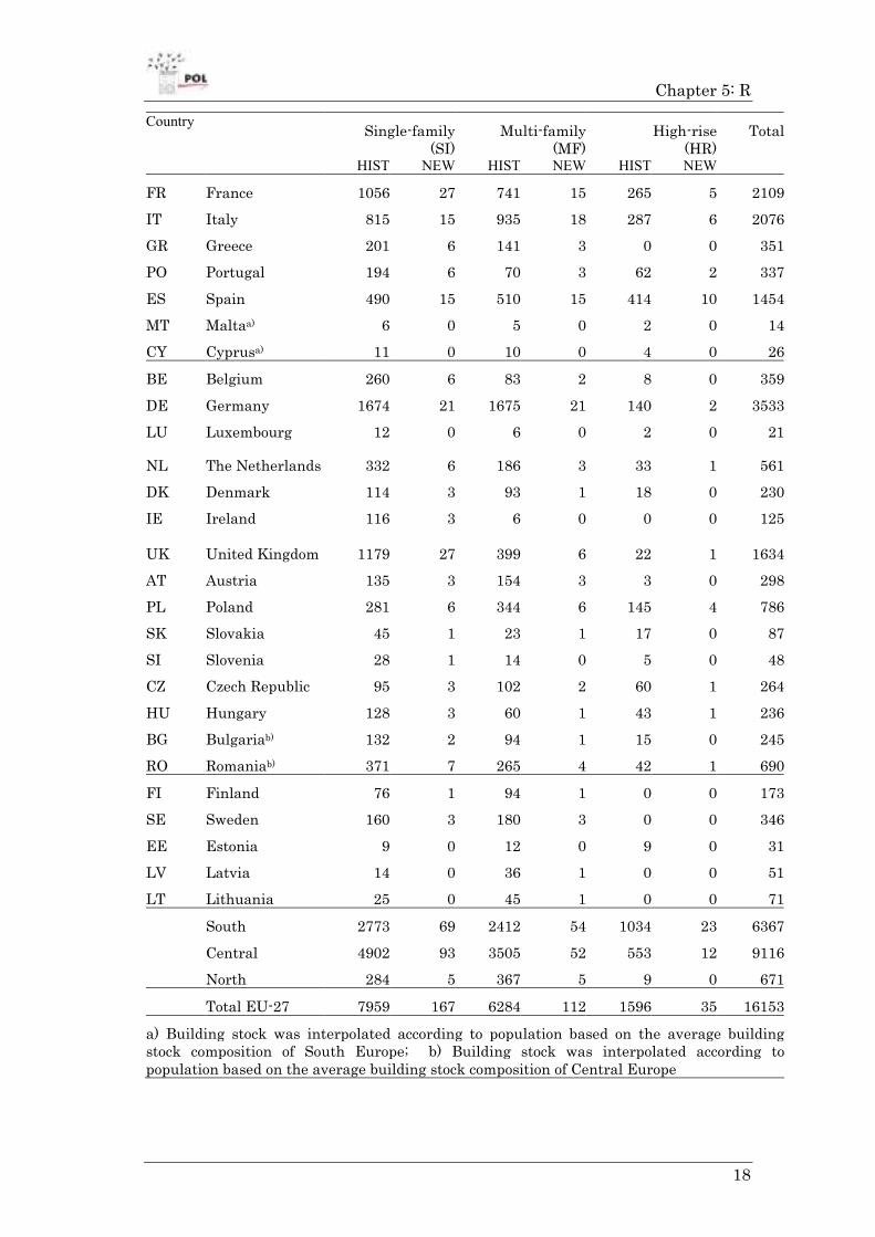
Table Table Table Table 3333: building for the EU 27 Member States in 2006 (Source: Uhilein and Eder 2010): building for the EU 27 Member States in 2006 (Source: Uhilein and Eder 2010): building for the EU 27 Member States in 2006 (Source: Uhilein and Eder 2010): building for the EU 27 Member States in 2006 (Source: Uhilein and Eder 2010)

Table 3 above displays the building stock assumed for the EU27 Member States in 2006. The demolition, construction and renovation cycles induce an increase of the building stock energy efficiency, which is subdivided in four different energy efficiency levels from 0 to 3. Whenever a construction activity takes place, the energy efficiency level is upgraded to the one of the corresponding year by differentiating on the basis of the type of the construction activity that has taken place.

a) b)

Figure Figure Figure Figure 5555: a) energy efficiency levels assumed for the reference: a) energy efficiency levels assumed for the reference: a) energy efficiency levels assumed for the reference: a) energy efficiency levels assumed for the reference scenario for the EU27; b) scenario for the EU27; b) scenario for the EU27; b) scenario for the EU27; b) cost structure for housing assumed in the reference scenariocost structure for housing assumed in the reference scenariocost structure for housing assumed in the reference scenariocost structure for housing assumed in the reference scenario (Source: Uhilein and Eder (Source: Uhilein and Eder (Source: Uhilein and Eder (Source: Uhilein and Eder 2009)2009)2009)2009)

Figure 5 shows the energy efficiency levels assumed in the reference scenario for EU27. The energy efficiency level 0 is present in the building stock until 2015. Level 1 phases in from 1974 and in 2000, the starting year of our simulation, and it covers the largest share, i.e. around 60%. Level 2 appears in 1991 and in 2000 only covers around 6% of the building stock. In the reference scenario, it is assumed that EE level 3 never occurs. The graph b) in Figure 5 shows how the main cost elements of the household expenditure for housing from 2000 to 2060.

A further step in the model consists in the quantification of the energy demand of the building stock for each country. This step was performed with the EPIQR model that quantifies the energy demand of a specific building type on the basis of the U-values, i.e. a coefficient that quantifies the heat loss through specific building elements like windows for instance, or on the basis of thickness, i.e. cm, of insulation applied in roofs and walls.

0

5000

10000

15000

20000

25000

30000

35000

40000

2000

2010

2020

2030

2040

2050

2060

Mio. m2 living area

EE 3

EE 2

EE 1

EE 0

0

500000

1000000

1500000

2000000

2500000

3000000

2000

2010

2020

2030

2040

2050

2060

Total cost [Mio. EUR]

Roof refurbishment

Window refurbishment

Energy

Major renovation

Construction

Chapter 5: R

20

Zone EE level Window refurbishment

Roof refurbishment

Wall refurbishment

North 0 Existing No additional insulation No additional insulation

1 U-value 1.6 14 cm additional insulation

8 cm additional insulation





Central 0 Existing No additional insulation No additional insulation







South 0 Existing No additional insulation No additional insulation







Table Table Table Table 4444: U: U: U: U----values corresponding to the energy efficiency level assumed for Northern, values corresponding to the energy efficiency level assumed for Northern, values corresponding to the energy efficiency level assumed for Northern, values corresponding to the energy efficiency level assumed for Northern, Central and Southern European countries (Source: Uhilein aCentral and Southern European countries (Source: Uhilein aCentral and Southern European countries (Source: Uhilein aCentral and Southern European countries (Source: Uhilein and Edernd Edernd Edernd Eder 2010 2010 2010 2010))))

Table 4 displays the U-values and cm of thickness of insulation assumed for the three regional clusters, i.e. North, Central and South of Europe, which are used to convert the energy efficiency levels in to energy demand.

The last step consists in converting the demand for construction materials and elements as well as the energy demand in to monetary expenditure. The costs related to the renovation and refurbishment activities were calculated for each EU country by taking Germany as a reference country and by applying a building cost index (BKI (Ed.) 2009). For the energy expenditure, the energy demand was first defined in terms of energy carriers using the energy mix specified in Nemry et al 2010 and subsequently converted in to energy expenditure by considering appropriate energy prices and taxation for each EU country (IEA) (Nemry et al. 2010; International Energy Agency 2007). The conversion of the energy consumption in to green house gases emissions is then obtained using conversion factors available in publicly available as well as commercial databases (ELCD II and Ecoinvent v2).

The building stock model was applied to analyse three different scenarios: the Reference scenario, the EPBD scenario and the cost optimal scenario. All the scenarios start in 2007. In the first scenario, i.e. EPBD, the policy measures that

Chapter 5: R

21

are currently in place in the EU are modelled. In more details, the two alternative scenarios analysed in this study make the following assumptions:

1. Reference scenario: in this reference scenario total living area increases at 1.52% annually, thus the total residential building stock in 2060 is about 2.5 times higher than in 2000. In addition, an annual GDP growth rate of 1.6% and a labour productivity growth rate of 1.8% are assumed for the whole period 2000-2060 (European Commission 2009).

2. EPBD scenario: from 2007 to 2011 for all new buildings, the major renovation of high-rise buildings, and 50% of the multi-family buildings (1000 m2 threshold), the energy efficiency level 2 is assumed. From 2012 on, all new construction and major renovation activities are performed according to energy efficiency level 2, i.e. the remaining 50% of the multi-family buildings is also in the scope of the EPBD. From 2014 on, energy efficiency level 3 phases in with an increasing share until 2016. From 2017, on energy efficiency level 3 is applied to all construction and major renovation activities.

3. Cost optimal: this scenario assumes that from 2009 on, all the renovation and refurbishment activities attain a cost-optimal energy efficiency level, which is defined as the energy efficiency level at which the annual costs (composed of capital/investment cost and energy cost savings) are the lowest.

The three scenarios, reference, EPBD and cost optimal are modeled in the MRIO model as an exogenous change of the household final demand for construction materials, building elements, energy, machinery and services, including construction services and other services like real estate. For this case study, the MRIO model based on Exiobase has been used to quantify the economy wide environmental and socio economic implications of the same scenarios analysed by the IPTS Building study. The use of a multi regional interindustry model permits the quantification of the indirect effects, i.e. effects on the rest of the economy, as well as of the trade related impacts.

For each of these alternative scenarios we will take into account the redistribution effects, in the sense that additional investments for renovation and refurbishment activities will be funded reducing the expenditure on other goods and services and that savings due to lower consumption of energy will be spent.

4.2 Private transport

For the transport activity, the scenarios analyzed in this study refer to the implementation of an incentive mechanism aiming at improving the environmental profile of the European passenger vehicle fleet. The scenarios are derived from an existing study conducted at the IPTS in 2009, which carries out a comprehensive environmental and socio-economic assessment of two policy options at the EU level: a registration tax system and a scrappage system (Nemry et al. 2009). The analysis of such complex policy issues required the utilization of a modelling framework able to capture the interaction between the

Chapter 5: R

22

consumers, that purchase, use and dispose a vehicle, the automotive industry production system, which is characterized by the use of large amounts of basic materials as well as the remaining sectors that supply the material inputs to the main production activity. The IPTS Impro-car study utilized a modelling framework based on the coherent combination of four analytical tools: Tremove, i.e. a transport policy assessment model, a Materials module with information about the material composition, the end-of-life of the vehicles and the spare parts in the EU27, an aggregated Input-Output model for the EU27, to quantify the interindustry indirect effects and a life-cycle assessment module, i.e. Impro car, to quantify the environmental impacts associated with material extraction and processing. The following picture, Figure 6, gives a schematic representation of the modelling framework.

Figure Figure Figure Figure 6666: modelling framework: modelling framework: modelling framework: modelling framework of the Impro of the Impro of the Impro of the Impro----Cars study (Source: Nemry et al 2010)Cars study (Source: Nemry et al 2010)Cars study (Source: Nemry et al 2010)Cars study (Source: Nemry et al 2010)

Tremove is a policy assessment model that quantifies the transport demand, the modal shifts, the vehicle stock renewal, the emissions of air pollutants and the welfare level associated to an assumed transport and environment policies, i.e. road pricing, public transport pricing, emission standards, subsidies for cleaner cars etc4. Once a specific transport policy scenario is assumed, the Tremove output, e.g. vehicle stock among others, is used as an input for the other modules.

4 See Del. III 4 C 2 for a more detailed description of the Tremove architecture

Chapter 5: R

23

0

50

100

150

200

250

300

350

1995 2000 2005 2010 2015 2020 2025 2030

Stock (106 vehicles) EURO6

EURO5

EURO4

EURO3

EURO2

EURO1

pre

Figure Figure Figure Figure 7777: EU passenger vehicle fleet evolution differentiated by the emission standard in : EU passenger vehicle fleet evolution differentiated by the emission standard in : EU passenger vehicle fleet evolution differentiated by the emission standard in : EU passenger vehicle fleet evolution differentiated by the emission standard in force (Source: Nemry et al 2009)force (Source: Nemry et al 2009)force (Source: Nemry et al 2009)force (Source: Nemry et al 2009)

Figure 7 portrays the evolution of the European vehicle fleet as in the Tremove reference scenario from 1995 to 2030. The total passenger vehicle stock increases over time, due to increasing transport demand.

The resulting vehicle stock is the input to the Materials module that quantifies the material flows indirectly generated by the transport demand, which includes the production of a vehicle and of the spare parts, i.e. tyres, batteries, lubricants etc., and by the disposal of the vehicle. The environmental impacts associated to those material flows are quantified with the Impro car life cycle assessment module. The Impro car module is based on the Ecoinvent database and quantifies the impacts in terms of mid point impact categories, i.e. Abiotic depletion, Global warming potential, Photochemical ozone creation potential, Acidification potential, Eutrophication potential and Bulk waste. The vehicle and fuel demand derived from Tremove represent the exogenous input to the Input Output model that uses those information, consistently mapped to the IO sectoral classification, to analyse the economy wide indirect effects of a change in the transport demand. The indirect effects depend on the interaction between the automotive industry, refinery industry and the rest of the economic sectors. In the IPTS Impro-car study, the Input Output model was used to quantify the socio economic impacts for the EU27 as a whole. The aim of the present exercise is therefore to improve the existing analysis by replacing the aggregated EU27 IO table with the Exiopol database. Besides the socio economic impacts, the use of the Exiopol database allows to quantify the indirect environmental impacts both for the EU and the Rest of the World including the impacts associated to the trade linkage between the EU and its main trading partners.

Tremove models transport demand as depending upon the vehicle purchase cost as well as on other vehicle related cost like insurance, tax, repairing and fuel. The baseline scenario reflects the existing vehicle costs structure and the associated transport demand at the EU level (Fiorello et al. 2009).

Chapter 5: R

24

0%

20%

40%

60%

80%

100%

2005 2010 2015 2020 2025 2030

vat

Oth tax

Oth cost

Rep cost

Fuel tax

Fuel cost

Reg tax

Pur cost

Figure Figure Figure Figure 8888: vehicle cost structure assumed in the Tremove baseline : vehicle cost structure assumed in the Tremove baseline : vehicle cost structure assumed in the Tremove baseline : vehicle cost structure assumed in the Tremove baseline

As for the emissions related to the use of the vehicle, they are calculated using the Well-to-Wheel method (Edwards et al. 2006). In particular, for the CO2 emissions the impact assessment of the regulation of CO2 emissions from cars is used as reference (EC, 2007)i, which assumes an emissions level of 160 g/km in 2006 and no further improvements beyond this year. Due to the imposition of higher emission standards in the period between 1995 and 2010, the passenger vehicle fleet experiences a renewal and progressively attains a better environmental profile. In this exercise however, the environmental impacts associated to the use phase of the vehicle will not be quantified, as the scope of the analysis is to extend and improve the existing analysis of the indirect environmental and socio economic impacts.

The scenarios analysed in the present study refer to the implementation of two policy measures, i.e. the feebate system and the scrappage policy. We propose the analysis of a set of three different scenarios resulting from a different combination of the two policy instruments. For the feebate system the pivot point is always assumed at 130 g CO2/km, but different types of feebate functions are assumed. For the scrappage system the vehicle replacement is assumed to occur when the vehicle is at least 8 years old. The three analysed scenario are as follows:

1. Scenario 1: a feebate system with the following bonus/malus scheme:

euro per vehicle

Big diesel 1293

Medium diesel 199

Small diesel -526

Big petrol 1800

Medium petrol 581

Small petrol -287

is combined with a scrappage system that gives a subsidy of 1000 euro to car owners who scrap their old car for a new one with better air emissions abatement technologies.

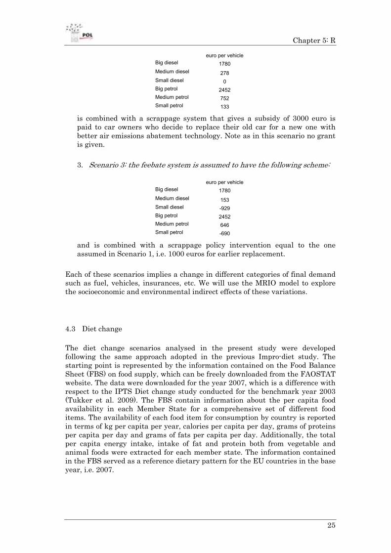
2. Scenario 2: a feebate system as follows:

Chapter 5: R

25

euro per vehicle

Big diesel 1780

Medium diesel 278

Small diesel 0

Big petrol 2452

Medium petrol 752

Small petrol 133

is combined with a scrappage system that gives a subsidy of 3000 euro is paid to car owners who decide to replace their old car for a new one with better air emissions abatement technology. Note as in this scenario no grant is given.

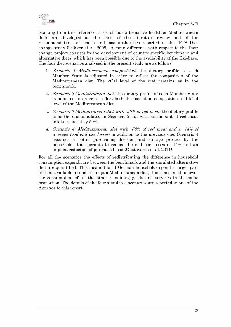
3. Scenario 3: the feebate system is assumed to have the following scheme:

euro per vehicle

Big diesel 1780

Medium diesel 153

Small diesel -929

Big petrol 2452

Medium petrol 646

Small petrol -690

and is combined with a scrappage policy intervention equal to the one assumed in Scenario 1, i.e. 1000 euros for earlier replacement.

Each of these scenarios implies a change in different categories of final demand such as fuel, vehicles, insurances, etc. We will use the MRIO model to explore the socioeconomic and environmental indirect effects of these variations.

4.3 Diet change

The diet change scenarios analysed in the present study were developed following the same approach adopted in the previous Impro-diet study. The starting point is represented by the information contained on the Food Balance Sheet (FBS) on food supply, which can be freely downloaded from the FAOSTAT website. The data were downloaded for the year 2007, which is a difference with respect to the IPTS Diet change study conducted for the benchmark year 2003 (Tukker et al. 2009). The FBS contain information about the per capita food availability in each Member State for a comprehensive set of different food items. The availability of each food item for consumption by country is reported in terms of kg per capita per year, calories per capita per day, grams of proteins per capita per day and grams of fats per capita per day. Additionally, the total per capita energy intake, intake of fat and protein both from vegetable and animal foods were extracted for each member state. The information contained in the FBS served as a reference dietary pattern for the EU countries in the base year, i.e. 2007.

Chapter 5: R

26

The Exiobase refers to the base year of 2000, so in order to derive a benchmark for our simulations, the vector of the final demand in the MRIO model has been rescaled using the consumption growth rates for the period 2000-2007 derived from the corresponding FBS. For the simulation exercise we therefore assume that the vector of the final demand in the MRIO model corresponds to the existing household diet.

Figure 1 shows the dietary pattern as derived from the FBS for each EU country in 2007. In addition to the overall level of kCal per capita in each country, the graph also shows the contribution of main food product, i.e. aggregated with respect to the Exiobase classification. In addition to the existing food consumption patterns in each EU country, the graph also includes an additional bar showing the proportion of the Mediterranean diet, which is assumed to be the reference diet to improve the overall European nutritional profile.

Figure Figure Figure Figure 9999: benchmark diet: benchmark diet: benchmark diet: benchmark dietary profiles of the EU Member Statesary profiles of the EU Member Statesary profiles of the EU Member Statesary profiles of the EU Member States

Together with a non negligible difference in the total intake of kCal per capita, which varies 8% around the mean, Figure 9 shows also a substantial difference in the diet composition. Largest relative differences are found for the consumption of meat, especially red meat, animal fat and fish.

cereals sugars Oilcrops+Vegetable

oils Alcohol Red meat Pigmeat Poultry

Other meat Dairy

Animal fat Fish

SD (kCal) 183 89 148 62 47 68 22 20 91 82 34 Mean (kCal) 1383 373 432 198 66 206 79 33 402 158 48 Coeff. Variation 13% 24% 34% 31% 72% 33% 28% 61% 23% 52% 71%

0 1000 2000 3000 4000 5000

Bulgaria

Slovakia

Latvia

Sweden

Cyprus

Estonia

Finland

Slovenia

Czech Republic

Spain

Netherlands

Mediterranean

Denmark

Poland

Lithuania

United Kingdom

Romania

Hungary

France

Germany

Portugal

Malta

Ireland

Italy

Luxembourg

Belgium

Greece

Austria

KCal per capita

Other cereals, starchyroots, pulses, treenuts,vegetables, fruits

Rice

Sugar & Sweeteners

Oilcrops

Vegetable Oils

Alcoholic Beverages

Bovine Meat

Other meats

Pigmeat

Poultry Meat

Dairy

Animal fats, eggs

Fish

Chapter 5: R

27

Table Table Table Table 5555: variation : variation : variation : variation in the EU in the EU in the EU in the EU of the kCal intake of the kCal intake of the kCal intake of the kCal intake fromfromfromfrom different different different different food itemsfood itemsfood itemsfood items

The following graph, i.e. Figure 10, compares the total intake of kCal per capita in each EU country with the ratio of the kCal intake from vegetable and the kCal from meat. The scatter graph also report the population size for each country measured by the size of the bubble. The red line indicates the value of the kCal Vegetable, kCal Meat ratio, which corresponds to the Mediterranean diet assumed for this study.

Figure Figure Figure Figure 10101010: kilo Calories from Vegetables compared : kilo Calories from Vegetables compared : kilo Calories from Vegetables compared : kilo Calories from Vegetables compared

Figure 10 shows the indirect relationship between the total calorie intake and the amount of vegetables over meat products, i.e. the larger the meat intake as compared to the vegetable intake the higher is the total intake of calories. It is also interesting to notice that the largest part of the EU population is below the Mediterranean threshold. It must be emphasised that the FBS report data about the apparent consumption, i.e. production plus import plus stock minus export, which is certainly higher than the actual per capita intake of calorie as it does not take into account losses occurring both during the transport, storage, processing and consumption of food. For this reason one of the four scenarios that will be analysed in this paper will assume a drastic reduction of the food end use losses.

0

1

2

3

4

5

6

7

2500 2700 2900 3100 3300 3500 3700 3900 4100

kCal per capita

kCal Veg./kCal Meat

Mediterrenean

diet

Chapter 5: R

28

Starting from this reference, a set of four alternative healthier Mediterranean diets are developed on the basis of the literature review and of the recommendations of health and food authorities reported in the IPTS Diet change study (Tukker et al. 2009). A main difference with respect to the Diet-change project consists in the development of country specific benchmark and alternative diets, which has been possible due to the availability of the Exiobase. The four diet scenarios analysed in the present study are as follows:

1. Scenario 1 Mediterranean composition: the dietary profile of each Member State is adjusted in order to reflect the composition of the Mediterranean diet. The kCal level of the diet remains as in the benchmark.

2. Scenario 2 Mediterranean diet: the dietary profile of each Mamber State is adjusted in order to reflect both the food item composition and kCal level of the Mediterranean diet.

3. Scenario 3 Mediterranean diet with -50% of red meat: the dietary profile is as the one simulated in Scenario 2 but with an amount of red meat intake reduced by 50%;

4. Scenario 4: Mediterranean diet with -50% of red meat and a -14% of average food end use losses: in addition to the previous one, Scenario 4 assumes a better purchasing decision and storage process by the households that permits to reduce the end use losses of 14% and an implicit reduction of purchased food (Gustavsson et al. 2011).

For all the scenarios the effects of redistributing the difference in household consumption expenditure between the benchmark and the simulated alternative diet are quantified. This means that if German households spend a larger part of their available income to adopt a Mediterranean diet, this is assumed to lower the consumption of all the other remaining goods and services in the same proportion. The details of the four simulated scenarios are reported in one of the Annexes to this report.

Chapter 5: R

29

5 Results discussion

5.1 Energy efficiency in buildings

In this section the indirect5 effects measured in terms of greenhouse gas (GHG) emissions, value added and employment for each of the scenario described in section 4.1 are presented.

In general terms, all the indicators considered in this study show a decreasing trend. This is mainly due to the 'redistribution effect' of household disposable income. In fact, we do not assume any public financial intervention aiming at promoting building renovation intervention so both in the EPBD and in the FCOA scenarios the higher expenditure devoted to the building renovation is financed by reducing the consumption of other categories, e.g. food and services. Given that on average the consumption categories related to building renovation activities are less intensive in terms of GHG emissions, employment and value added, than the other categories, a reduction in total emissions, employment and value added takes place.

Figure 11, Figure 13 and Figure 15 show the impacts generated in EU27 and figures Figure 12, Figure 14 and Figure 16 summarize the effects in the 'rest of the world'. All the results are expressed in terms of absolute changes, i.e. Mt of CO2 eq., with respect the reference scenario.

5 As previously reported, we use the MRIO model to quantify the indirect effects generated on economy and environment. This means that we do analyse the effects of the scenarios on all the economic sectors, but we do not include the changes in household emissions induced by the higher energy efficiency levels promoted by the simulated policy interventions.

Chapter 5: R

30

Similarly to the trends quantified for the FCOA scenario in the paper by Uihlein and Eder (2010), also this analysis shows a largely decreasing trend for greenhouse gas emissions in EU27 between 2007 and 2020 and between 2028 and 2040.

-200

-180

-160

-140

-120

-100

-80

-60

-40

-20

0

2000

2004

2008

2012

2016

2020

2024

2028

2032

2036

2040

2044

2048

2052

2056

2060

Mtons CO2 equivalents

EPBD FCOA

Figure Figure Figure Figure 11111111:::: Trends on GHG emissions in EU27 ( Trends on GHG emissions in EU27 ( Trends on GHG emissions in EU27 ( Trends on GHG emissions in EU27 (MMMMtons of CO2 equivalents)tons of CO2 equivalents)tons of CO2 equivalents)tons of CO2 equivalents)

During these periods refurbishment is encouraged and the household investments in buildings generate a reduction of the income available for the consumption of other goods and services and a consequent reduction in GHG emissions. During the periods when no refurbishment activity takes place, the household disposable income and associated consumption return to the pre-reform level, which leads to an increase of GHG emissions. However, the emissions reductions calculated under the FCOA scenario are always larger than those calculated under the EPBD scenario. The EPBD scenario in fact assumes that less renovation activity takes place during the considered period. Moreover, since the EPBD scenario assumes an almost constant trend of investments in building, the GHG emission reduction results to have a smoother and almost linear decreasing trend.

The GHG emissions in the 'rest of the world' show a decreasing trend under both the EPBD and the FCOA scenarios. However, as shown in Figure 12, between 2020 and 2030 the GHG emissions related to the FCOA scenario are higher than the emissions quantified for the Reference and the EPBD scenarios. The explanation for this difference is also in this case based on the redistribution of disposable income, i.e. once no refurbishment activity need to be financed the disposable income returns to its pre-intervention level and this leads to an

Chapter 5: R

31

increase of imports and of GHG emissions abroad. In addition, the reduction in energy consumption (and imports) due to the enhancement of environmental performance of buildings also contributes to reduce GHG emissions abroad.

-70

-60

-50

-40

-30

-20

-10

0

10

20

30

2000

2004

2008

2012

2016

2020

2024

2028

2032

2036

2040

2044

2048

2052

2056

2060

Mtons CO2 equivalents

EPBD FCOA

Figure Figure Figure Figure 12121212:::: Trend on GHG in the Trend on GHG in the Trend on GHG in the Trend on GHG in the ''''Rest of the WorldRest of the WorldRest of the WorldRest of the World'''' ( ( ( (MMMMtons of CO2 equivalents)tons of CO2 equivalents)tons of CO2 equivalents)tons of CO2 equivalents)

Value added has a similar trend both for the EU27 and for the 'rest of the world'.

Also in this case the 'redistribution effect' of disposable income determines a reduction of the total value added generated up to 2060 both in the EPBD and in the FCOA scenarios, compared to the BAU scenario. As previously reported, the building sector is less value added intensive than the other economic sectors and then allocating a larger share of the overall household expenditure to the building sector leads to an overall reduction in terms value added.

The relevance of the redistribution effect in this scenario is confirmed by the trend of the value added under the FCOA scenario in the period between 2020 and 2030. As there is no additional expenditure for building renovation activities the redistribution of the disposable income according to the pre-reform consumption pattern generates an increase of value added. A similar trend characterises the results for the 'rest of the world' that is influenced by European expenditures for imported products.

Chapter 5: R

32

-80.000

-70.000

-60.000

-50.000

-40.000

-30.000

-20.000

-10.000

0

10.000

20.000

30.000

2000

2004

2008

2012

2016

2020

2024

2028

2032

2036

2040

2044

2048

2052

2056

2060

EPBD FCOA

Figure Figure Figure Figure 13131313:::: Trend on value added iTrend on value added iTrend on value added iTrend on value added in EU27n EU27n EU27n EU27

-70.000

-60.000

-50.000

-40.000

-30.000

-20.000

-10.000

0

10.000

20.0002000

2004

2008

2012

2016

2020

2024

2028

2032

2036

2040

2044

2048

2052

2056

2060

EPBD FCOA

Figure Figure Figure Figure 14141414:::: Trend on value added in the Trend on value added in the Trend on value added in the Trend on value added in the ''''Rest of the WorldRest of the WorldRest of the WorldRest of the World''''

Chapter 5: R

33

All the three scenarios considered in this study do not generate variations on employment during the last 20 years. This result strongly depends on the assumed labour productivity growth rate (see section 4.1).

For the EPBD scenario almost no difference is measured with respect to the reference scenario. That is because investments in buildings are spread during the entire period and fewer variations take place in the sectors of household expenditures and then smaller variations take place on employment.

Similarly to the trends previously reported for GHG and value added, employment changes in the FCOA scenario are largely driven by the 'redistribution effect'. During the period of building renovation, less income is available for the purchase of less employment-intensive goods and services and therefore total employment falls.

The results for employment offer an interesting insight on the differences of sectoral labour intensity in Europe and the 'rest of the world'. In fact, in this case both the EPBD and the FCOA scenarios are characterised by a loss of employment when compared to the reference scenario. On the one hand, a larger share of the overall household disposable income is allocated to building renovation that is part of the domestic demand and this reduces the import demand and the associated employment. On the other hand, the imported goods are on average more labour intensive than domestic production, which contributes to the employment reduction in the 'rest of the world'.

-1.200

-1.000

-800

-600

-400

-200

0

200

400

600

2000

2004

2008

2012

2016

2020

2024

2028

2032

2036

2040

2044

2048

2052

2056

2060

EPBD FCOA

Figure Figure Figure Figure 15151515:::: Trend on employment in EU27Trend on employment in EU27Trend on employment in EU27Trend on employment in EU27

Chapter 5: R

34

-4.000

-3.500

-3.000

-2.500

-2.000

-1.500

-1.000

-500

0

500

1.000

1.500

2000

2004

2008

2012

2016

2020

2024

2028

2032

2036

2040

2044

2048

2052

2056

2060

EPBD FCOA

Figure Figure Figure Figure 16161616:::: Trend on employment in the Trend on employment in the Trend on employment in the Trend on employment in the ''''Rest of the WorldRest of the WorldRest of the WorldRest of the World''''

5.2 Private transport

Table 6 summarizes the economic and environmental effects of the three simulated policy interventions described in section 4.2. The differences with respect to the reference scenario are reported in percentage and are calculated as the sum of all the effects measured for the period between 2006 and 2020. Similarly to the 'energy efficiency in buildings' scenario, these results only refer to the indirect effects generated by the policy interventions, i.e. the sum of the economy wide impacts generated by variations in the final demand. Due to the particular nature of the transport scenarios we decided to extend the number of environmental indicators used for the analysis. In addition to GHG emissions, energy use, biomass, unused biomass, water, land and acidifying emissions, i.e. SOx, NH3 and NOx, are also used to measure the impact of the simulated policies.

Table Table Table Table 6666:::: Cumulative change with respect to the Reference scenario for EU27 (%) Cumulative change with respect to the Reference scenario for EU27 (%) Cumulative change with respect to the Reference scenario for EU27 (%) Cumulative change with respect to the Reference scenario for EU27 (%)

Scenario Value Added

Employment Energy Use

Biomass Unused Biomass

Water Land GHG emissions

Acidifying Emissions

1 0.76 1.04 -8.38 -1.67 -1.65 -1.20 -1.11 0.25 -0.53

2 -0.37 0.67 -17.51 -14.58 -14.88 -14.40 -12.03 1.08 -6.49

3 1.06 1.43 -11.46 -2.19 -2.16 -1.50 -1.43 0.31 -0.69

Chapter 5: R

35

Table 6Error! Reference source not found.Error! Reference source not found.Error! Reference source not found.Error! Reference source not found. reports the aggregate results for the three analysed scenarios. The largest differences with respect to the reference scenario are measured for Scenario 2, where total use of biomass, unused biomass, energy and water use decrease by more than 14% in the period between 2006 and 2020. In scenarios 1 and 3 the largest variations take place in the energy use that decreases by 8.38% and 11.46% respectively. The reduction measured in the category 'energy use' depends on the lower consumption of energy feedstock in the refinery sector, which in turn is due to higher energy efficiency of the vehicle fleet. Smaller reductions are measured for acidifying emissions that decrease by 0.53% in Scenario 1, 6.49% in scenario 2 and 0.69% in Scenario 3. The increase of GHG emissions depends mainly on the production of steel used for the manufacturing of new cars.

The impacts on the category 'value added' and 'employment' are relatively small. Employment is the category that is mostly affected and a detailed analysis, disaggregated by economic sector, is reported in the following group of tables. For each of the scenarios the tables list the sectors that are most affected either by a reduction or an increase of the employment.

Scenario 1

Sector Percentage Variation

Manufacture of motor spirit (gasoline) -5.65

Retail sale of automotive fuel -4.30

Extraction of crude petroleum and services related to crude oil extraction, excluding surveying

-2.50

Extraction, liquefaction, and regasification of other petroleum and gaseous materials

-0.85

Manufacture of coke oven products -0.79

Table Table Table Table 7777:::: Largest percentage reductions Largest percentage reductions Largest percentage reductions Largest percentage reductions in employmentin employmentin employmentin employment–––– Top five sectors, scenario 1 Top five sectors, scenario 1 Top five sectors, scenario 1 Top five sectors, scenario 1

Sector Percentage variation

Manufacture of motor vehicles, trailers and semi-trailers 3.07

Sale, maintenance, repair of motor vehicles, motor vehicles parts, motorcycles, motor cycles parts and accessories

2.59

Insurance and pension funding, except compulsory social security

1.12

Casting of metals 1.06

Manufacture of basic iron and steel 0.51

Table Table Table Table 8888:::: Largest percentage increases Largest percentage increases Largest percentage increases Largest percentage increases –––– in emplin emplin emplin employmentoymentoymentoyment Top five sectors, scenario 1 Top five sectors, scenario 1 Top five sectors, scenario 1 Top five sectors, scenario 1

Scenario 2


Chapter 5: R

36



Extraction of crude petroleum and services related to crude oil extraction, excluding surveying

-4.73

Private households with employed persons -1.94

Extraction, liquefaction and regasification of other petroleum and gaseous materials

-1.66

Table Table Table Table 9999:::: Largest percentage reductions Largest percentage reductions Largest percentage reductions Largest percentage reductions ––––in employmentin employmentin employmentin employment Top five sectors, scenario Top five sectors, scenario Top five sectors, scenario Top five sectors, scenario 2222




Sale, maintenance, repair of motor vehicles, motor vehicles parts, motorcycles, motor cycles parts and accessories 3.40


Aluminium product 2.91

Table Table Table Table 10101010:::: Largest percentage increases Largest percentage increases Largest percentage increases Largest percentage increases ––––in employmentin employmentin employmentin employment Top five sectors, scenario 2 Top five sectors, scenario 2 Top five sectors, scenario 2 Top five sectors, scenario 2

Scenario 3




Extraction of crude petroleum and services related to crude oil extraction, excluding surveying -3.42

Extraction, liquefaction and regasification of other petroleum and gaseous materials -1.16

Manufacture of coke oven products -1.08

Table Table Table Table 11111111:::: Largest percentage reductions Largest percentage reductions Largest percentage reductions Largest percentage reductions ––––in employmentin employmentin employmentin employment Top five sectors, scenario 3 Top five sectors, scenario 3 Top five sectors, scenario 3 Top five sectors, scenario 3



Sale, maintenance, repair of motor vehicles, motor vehicles parts, motorcycles, motor cycles parts and accessories 3.58

Insurance and pension funding, except compulsory social security 1.61



Table Table Table Table 12121212:::: LargLargLargLargest percentage increases est percentage increases est percentage increases est percentage increases ––––in employmentin employmentin employmentin employment Top five sectors, scenario 3 Top five sectors, scenario 3 Top five sectors, scenario 3 Top five sectors, scenario 3

Chapter 5: R

37

The employment impacts reported in Tables 7 to 12 are consistent with the simulated policies. For all the sectors related to fuel use for private transport a reduction of employment is measured. While for the sectors related to car production and use, with the exception of fuel use, an increase is measured. The largest relative variations have been obtained for Scenario 2. The 'Manufacture of motor spirit (gasoline)' and the 'Retail sale of automotive fuel', for example, would experience a reduction of employment equal to 10.79 and 8.49 percent respectively. On the contrary for the sector 'Manufacture of motor vehicles, trailers and semi-trailer' an increase in labour input by almost 19.5% is reported.

Since the main objective of the feebate and the scrappage policies was to promote the substitution between old and new cars, with better efficiency and abatement technologies, the reduction of employment in the sectors related to the fuel production and the labour increases in the sectors of vehicles production, confirm the efficiency of these policies.

Regarding the 'rest of the world' on the basis of the results reported in Table 13, employment is the most affected variable in the 'rest of the world'. The growth in the demand for new cars in EU27 generates an increase in the production of cars and components in the 'rest of the world'. However, the negative variations reported for the value added depend on the difference in capital intensity between the refinery sector and the car manufacturing sector. The petroleum extractive sector is 10 times more capital intensive, i.e. capital use divided by euro of gdp generated by the sector, than the car manufacturing sector; also in absolute term the crude oil extractive sector uses 4 times more capital than the car manufacturing sector. Therefore the increasing car demand does not compensate the value added reduction due to lower capital use that takes place in the sectors related to oil extraction and oil production.





Acid Emissions

1 -0.30 0.00 -0.40 -0.22 -0.26 -0.30 -0.19 -0.16 -0.30

2 0.00 0.15 -0.12 -0.22 -0.54 -0.15 -0.13 0.40 0.07

3 -0.45 -0.15 -0.55 -0.31 -0.36 -1.50 -0.26 -0.23 -0.30

Table Table Table Table 13131313:::: Cumulative change with respect the baseline Rest of the World (%) Cumulative change with respect the baseline Rest of the World (%) Cumulative change with respect the baseline Rest of the World (%) Cumulative change with respect the baseline Rest of the World (%)

Similarly to EU27, the reduction on fuel consumption and the changes in the composition of final demand also contribute to the reduction of the environmental impacts in the 'rest of the world'. As reported in Table 13, for land, biomass, unused biomass, water and energy use a negative variation is measured in all the three scenarios considered in our analysis.

Chapter 5: R

38

5.3 Diet changeDiet changeDiet changeDiet change

Table 14 summarizes the effects of the four scenarios described in section 4.3 on several economic and environmental variables for the EU27. The figures are reported as changes with respect the base year 2007. Also for the scenarios presented in this section a larger set of economic and environmental indicators is considered.





Acid Emissions

1 -0.26 -2.53 -0.75 1.84 7.59 -2.38 -5.45 -0.60 -1.84

2 -0.27 -2.56 -0.76 0.03 5.61 -3.06 -6.62 -0.85 -2.40

3 -0.25 -2.66 -0.63 -2.90 3.63 -5.73 -7.59 -1.86 -7.74

4 -0.24 -2.86 -0.64 -15.16 -16.03 -22.03

-18.66 -2.24 -6.36

Table Table Table Table 14141414:::: Percentage variations (%) from baseline year Percentage variations (%) from baseline year Percentage variations (%) from baseline year Percentage variations (%) from baseline year –––– Diet Change, EU27 Diet Change, EU27 Diet Change, EU27 Diet Change, EU27

For all the scenarios considered in this study, most of the variables show a reduction. Only small increases are measured for the category 'Biomass', in scenarios 1 and 2, and for the category 'Unused Biomass', in scenarios 1, 2 and 3. These results depend on the one hand on the increasing consumption of fruits, vegetable oils and vegetables because the Mediterranean diet is assumed to be extended to all the European countries. However, the lower consumption of meat reduces the need of biomass for animal feeding, which counteracts the previous effect. For the scenarios 3 and 4 the quantity of biomass diminishes mainly because of the reduction of 50% of the intake of red meat and for the better food-related waste management at the household level.

One of the main findings of this simulations is the large reduction measured in land and water use that, in scenario 4, decrease by more than 19% and 22% respectively. Moreover, the reduction of meat consumption in scenario 3 leads to a decrease of 7.74% in acid emissions.

In general terms, the diet change scenarios produce larger variations in the environmental variables than in the economic variables. As reported in Table 14, the reduction in employment is less than 2.9% for all the four scenarios considered in the study and value added variation are around 0.25%.

Table 15 summarizes the effects generated in the 'rest of the world' by the four diet change scenarios reported above and applied to EU27.





Acid Emissions

1 -0,003 0,042 0.00 0.13 0.42 0.05 0.10 0.02 0.04

2 -0,004 0,031 -0.01 0.10 0.35 0.04 0.08 0.01 0.03

Chapter 5: R

39

3 -0,022 -0,015 -0.03 -0.02 0.13 -0.05 -0.03 -0.03 -0.05

4 -0,038 -0,088 -0.04 -0.17 -0.36 -0.13 -0.12 -0.05 -0.08

Table Table Table Table 15151515 Percentage variations (%) from bPercentage variations (%) from bPercentage variations (%) from bPercentage variations (%) from baseline year aseline year aseline year aseline year –––– Diet Change, Rest of the World Diet Change, Rest of the World Diet Change, Rest of the World Diet Change, Rest of the World

The results reported in Table 14 for the 'rest of the world' are largely smaller than the variations measured for EU27. Most of the food value chain is located inside the EU and, therefore, these scenarios have little trade related impacts.

Chapter 5: R

40

6 Conclusions

The present report proposes the use of the Exiopol database for the analysis of a number of scenarios relating to sustainable private consumption. Three distinct areas of private consumption are analysed in details, i.e. food consumption, private transport and energy use in residential buildings. The results of already existing sector specific bottom-up analyses in these areas of consumption are extended to the rest of the economy using an Input Output model based on the Exiopol database. In this context, the use of the Exiopol database permits to quantify the economy wide environmental and socio economic repercussions associated with each of the analysed scenario, including trade related impacts. The results of the analysis only include the indirect effects, i.e. those that indirectly follow a shock of the household final demand, and does not include the effects that are directly associated to a change in consumption behaviour, e.g. less CO2 emissions due to the use of a more efficient vehicle. The results are differentiated according to the geographical location, i.e. EU27 or the Rest of the World (RoW). In all the simulated scenarios a main assumption is that there is no public financial intervention, which implies that households must finance the additional expenditure necessary to shift to a more sustainable consumption profile, i.e. the additional investment in building renovation, by reducing the consumption in other categories. We assume a unitary elasticity of substitution between the different consumption categories that leads to redistribute the lower expenditure according to the consumption shares of each good or service.

Both the scenarios analysed for the residential sector show a reduction of the GHG emissions, which is due mainly to the lower level of production of the refinery sector. The income redistribution also plays a relevant role as the households must finance the intervention by reducing the consumption of other goods and services. The impacts measured for employment offer interesting insights on the differences of sectoral labour intensity in Europe and the RoW. Both the EPBD and the FCOA scenarios determine a loss of employment compared to the reference scenario as a larger share of the disposable income is allocated to the domestic demand, i.e. renovation activities, and this reduces the import demand that is on average more labour intensive than domestic production.

For private transport, we ran a number of scenarios all featuring a combination of two demand side policy measures, i.e. feebate and scrappage. As in the case of the building scenarios, the disposable income redistribution effects play a relevant role. The change in the consumption structure that is necessary to finance the purchase of a new car determines large reduction in the total use of biomass, unused biomass in the period between 2006 and 2020. The consumption of energy feedstock for the refinery sector also decreases substantially, while GHG emissions increase because of the manufacturing of new cars and vehicle part and components, i.e. steel. A relevant result is the loss of value added in the RoW that depends on the lower export of fuels to the EU; the refinery sector is indeed very capital intensive.

For food consumption, the simulated scenarios are all characterized by a shift of the main dietary profile of the EU27 Member States towards a Mediterranean

Chapter 5: R

41

diet. Moreover, as one of the main areas of environmental improvement for this consumption category is represented by a reduction of food losses, the last scenario, i.e. Scenario 4, assumes that the households are able to reduce waste losses by around 15%. The main findings are the changes in land use and water consumption. Both results depend on the reduction of meat consumption, i.e. less water and less land required for cultivating animal feed. Regarding socio economic impacts, a change in the dietary profile generates a reduction in total employment. The results measured for the RoW are largely smaller than those for the EU27 as most of the food value chain is located inside the EU. Nevertheless, the base year of the database is 2000 and this constitutes a limitation of the study especially with respect to the trade spill over impacts since the scale of trade has been increasing steeply in the last decade.

Chapter 5: R

42

List of references

Britz, W. Witzke, P. [eds.] (2008). CAPRI model documentation 2008: Version 2.

BKI (Ed.), Regionalfaktoren 2009 für Deutschland und Europa, Baukosteninformationszentrum Deutscher Architektenkammer, 2009

Criqui, P. (2001). POLES. Prospective Outlook on Long-term Energy Systems. Unité mixte de recherche du Centre National de la Recherche Scientifique et de l’Université Pierre Mendès France (UFR DGES), Grenoble, France.

De Ceuster, G., van Herbruggen, B., Ivanova, O., Carlier, K., Martino, A., Fiorello, D. (2007). TREMOVE. Service contract for the further development and application of the transport and environmental TREMOVE model Lot 1 (Improvement of the data set and model structure). FINAL REPORT.

Directorate-General for Economic and Financial Affairs of the European Commission 2009. Sustainability Report 2009 EUROPEAN ECONOMY 9. ISBN 978-92-79-11370-3. European Communities, 2009, Luxemburg

Eder P., Delgado L.S., (2006), Environmental impact of products (EIPRO) – Analysis of the life cycle environmental impacts related to the final consumption of the EU-25. European Commission, JRC-IPTS. EUR 22284 EN. Office for Official Publications of the European Communities, Luxembourg 2006. Available at: http://ec.europa.eu/environment/ipp/pdf/eipro_report.pdf

European Commission (2008). Communication from the Commissions to the European Parliament, the Council, the European Economic and Social Committee and the Committee of the Regions on the Sustainable Consumption and Production and Sustainable Industrial Policy. Action Plan. Brussels, 16.7.2008 COM(2008) 397 final

European Commission (2010). Report from the Commission to the European Parliament, the Council and the European Economic and Social Committee. Progress report on implementation of the Community’s integrated approach to reduce CO2 emissions from light-duty vehicles. Brussels, 10.11.2010 COM(2010) 656 final

European Commission, 2010. Regulation (EC) No 66/2010 OF THE EUROPEAN PARLIAMENT AND OF THE COUNCIL of 25 November 2009 on the EU Ecolabel

Eurostat: Statistical office of the European Union, http://epp.eurostat.ec.europa.eu, accessed at various dates in 2011.

ELCD II Core Data Sets, http://lca.jrc.ec.europa.eu, European Commission, 1995–2009.

Ecoinvent Database 1.2, Ecoinvent, Dübendorf, 2003–2004.

Edwards R, Larivé JF, Mahieu V, Rouveirolles P. Well-to-Wheels analysis of future automotive fuels and powertrains in the European context. European

Chapter 5: R

43

Commission DG JRC/IES, CONCAWE and EUCAR, 2006. Available at: http://ies.jrc.ec.europa.eu/WTW

European Commission (DG ECFIN) and the Economic Policy Committee (AWG). The 2009 Ageing Report : Economic and budgetary projections for the EU-27 Member States (2008-2060). EUROPEAN ECONOMY 2|2009. ISBN 978-92-79-11363-9. Downloadable at: http://ec.europa.eu/economy_finance/publications/publication14992_en.pdf

Fiorello D., De Stasio C., Köhler J., Kraft M., Newton S., Purwanto J., Schade B., Schade W., Szimba E. (2009): The iTREN-2030 reference scenario until 2030. Deliverable 4 of iTREN-2030 (Integrated transport and energy baseline until 2030). Project co-funded by European Commission 6th RTD Programme. Milan, Italy.

Gustavsson J. Cederberg C., Sonesson U., van Otterdijk R., Meybeck A. 2011. Global food losses and food waste extent, causes and prevention Food and Agriculture Organization of the United Nations, Rome, Italy.

Imhoff, M.L., Bounoua, L., Ricketts, T., Loucks, C., Harriss, R., Lawrence, W.T., 2004. Global patterns in human consumption of net primary production. Nature 429, 870–873.

International Energy Agency, Energy prices & taxes, Quarterly Statistics 2007, OECD/IEA, Paris, 2007.

Kletzan D., Köppl A., Kratena K., Schleicher S., Wüger M. 2006. Towards sustainable consumption: Economic modelling of mobility and heating for Austria. Ecological Economics, Volume 57, Issue 4, 1 June 2006, Pages 608-626

Kratena, K. and Streicher, G (2008). 'Macroeconomic Input-Output Modelling– Structures, Functional Forms and Closure Rules'. International Input-Output Association, Working Papers in Input-Output Economics, WPIOX 09-009

Maldonando E. (2011). Implementing the Energy Performance of Building Directive (EPBD). Featuring country reports 2010. ISBN 978-92-9202-090-3 EA-30-11-026-EN-C. Brussels April 2011. Available at: http://www.epbd-ca.org/Medias/Downloads/CA_Book_Implementing_the_EPBD_Featuring_Country_Reports_2010.pdf

Michaelis L., 2003. Sustainable consumption and greenhouse gas mitigation. Climate Policy, Volume 3, Supplement 1, November 2003, Pages S135-S146

Miller, R. E., Blair, P. D. (2009). Input-Output Analysis: Foundations and Extensions. Second edition. Cambridge University Press, Cambridge, United Kingdom.

Nash H.A., 2009. The European Commission's sustainable consumption and production and sustainable industrial policy action plan. Journal of Cleaner Production, Volume 17, Issue 4, March 2009, Pages 496-498

Navajas, E.; Mongelli, I. .; Kritzinger, S.; Helmreich, S.; Morgenstern, C.; Dennisen, T.; (2010): Deliverable 3 of LogMan project; Carbon Footprint (preliminary analysis). Funded by the European Commission 7th RTD Programme. Basel, Switzerland

Chapter 5: R

44

Nemry F., Uihlein A., Makishi Colodel C., Wittstock B., Braune A., Wetzel C., Hasan I., Niemeier S., Frech Y., Kreißig J. and Gallon N. (2008), Environmental improvement potentials of residential buildings (IMPRO-Building). European Commission, JRC-IPTS. EUR 23493 EN. Office for Official Publications of the European Communities, Luxembourg, 2008. Available at: http://ipts.jrc.ec.europa.eu/publications/pub.cfm?id=1744

Nemry, F.; Uihlein, A.; Colodel, C.M.; Wetzel, C.; Braune, A.; Wittstock, B.; Hasan, I.; Kreiszig, J.; Gallon, N.; Niemeier, S.; Frech, Y. 2010. Options to reduce the environmental impacts of residential buildings in the European Union-Potential and costs. Energy and Buildings, 42(7), 976-984

Nemry Francoise, Vanherleke Kris, Zimmer Wiebke, Uihlein Andreas, Genty Aurelien, Rueda Cantuche Jose, Mongelli Ignazio, Neuwahl Frederik, Delgado Sancho Luis, Hacker Florian, Seum Stefan, Buchert Matthias, Schade Wolfgang (2009). Feebate and Scrappage Policy Instruments - Environmental and Economic Impacts for the EU27. European Commission. JRC Publication n. JRC51094. ISBN: 978-92-79-12023-7. ISSN: 1018-5593. EUR 23896 EN. Available at: http://ipts.jrc.ec.europa.eu/publications/pub.cfm?id=2579

Neuwahl, F., Löschel, A, Mongelli, I, Delgado, L. (2008). Employment impacts of EU biofuels policy: Combining bottom-up technology information and sectoral market simulations in an input–output framework. Ecological Economics 68, 447-460.

OECD/IEA and AFD (2008), Promoting energy efficiency investments – Case studies in the residential sector. OECD/IEA, Paris. Available at: http://www.iea.org/w/bookshop/add.aspx?id=326

OJL 001 (2003), Directive 2002/91/EC of the European Parliament and of the Council of 16 December 2002 on the energy performance of buildings. Official Journal of the European Union L 001 (2003) 65-71. Available at: http://eur-lex.europa.eu/Result.do?RechType=RECH_celex&lang=en&code=32002L0091

Pyatt, G. (1994), Modelling Commodity Balances: A Derivation of the Stone Model. The Richard Stone Memorial Lecture, Part I, Economic Systems Research, 6(1), pp. 5-20.

Schafer A., Jacoby H.D., 2006. Experiments with a Hybrid CGE-MARKAL Model. Special issue #2 on Hybrid Modeling. The Energy Journal, pages: 171-177

Suh, S., 2004. Functions, commodities and environmental impacts in an ecological–economic model. Ecological Economics 40 (4), 451–467.

The Allen Consulting Group (2004), The energy efficiency gap – Market failures and policy options. Report to the Business Council for Sustainable Energy, the Australasian Energy Performance Contracting Association and the Insulation Council of Australia and New Zealand. The Allen Consulting, Melbourne 2004. Available at: http://www.aepca.asn.au/documents/EnergyEfficiencyGapFinalReport.pdf

Tukker, A., Bausch-Goldbohm, S., Verheijden, M., Koning, A., Kleijn, R., Wolf, O., Pérez Domínguez, I. (2009). Environmental Impacts of Diet Changes in the EU. Institute for Prospective Technological Studies, Seville, Spain.

Chapter 5: R

45

Tukker, A., Heijungs, R. (eds.) (2008) Technical Report: Definition study for the EE-IO database (D III 1 a 5).

Uihlein A & Eder P. (2009), Towards additional policies to improve the environmental performance of buildings. European Commission, JRC-IPTS. EUR 23775 EN. Office for Official Publications of the European Communities, Luxembourg 2009. Available at: http://ipts.jrc.ec.europa.eu/publications/pub.cfm?id=2079

Uihlein Andreas and Eder Peter (2009). Towards Additional Policies to Improve the Environmental Performance of Buildings. Part II: Quantitative Assessment. JRC Publication n. JRC53640 ISBN: 978-92-79-13734-1 ISSN: 1018-5593 EUR 24015 EN. Available at http://ipts.jrc.ec.europa.eu/publications/pub.cfm?id=2699

Uihlein, A.; Eder, P. 2010. Policy options towards an energy efficient residential building stock in the EU-27. Energy and Buildings, Volume 42(6), 791-798

Chapter 5: R

46

Annex: Contributors to the report

IPTS: Ignazio Mongelli, Iñaki Arto, Valeria Andreoni

TNO: Arnold Tukker

i EC Commission, 2007, Commission staff working document - Accompanying document to the Proposal from the Commission to the European Parliament and the Council for a Regulation to reduce CO2 emissions from passenger cars – Impact assessment (COM(2007)856final)

sustainable consumption patterns in eu27. a - feem-

Documents