U.S. Department of the Interior U.S. Geological Survey

SSuuttrraaPPrreepp A Preprocessor for SUTRA, a Model for Ground-Water Flow with Solute or Energy Transport

Open-File Report 02-376

Version of September 1, 2003 Latest version available at http://water.usgs.gov/nrp/gwsoftware

Front Cover: The “S”-shaped mesh was generated using SutraPrep. It consists of 42 blocks subdivided into 756 elements. Although this mesh is not typical of those encountered in hydrologic modeling, it demonstrates that a logically rectangular mesh can be geometrically complex.

U.S. Department of the Interior U.S. Geological Survey SutraPrep: A Preprocessor for SUTRA, a Model for Ground-Water Flow with Solute or Energy Transport By Alden M. Provost Open-File Report 02-376 Version of September 1, 2003 Reston, Virginia 2002

U.S. DEPARTMENT OF THE INTERIOR GALE A. NORTON, Secretary U.S. GEOLOGICAL SURVEY Charles G. Groat, Director The use of trade, product, or firm names in this report is for descriptive purposes only and does not imply endorsement by the U.S. Government. For additional information write to: SUTRA Support U.S. Geological Survey 431 National Center Reston, VA 20192 USA

Copies of this report can be purchased from: U.S. Geological Survey Branch of Information Services Box 25286 Denver, CO 80225-0286 USA

iii

PREFACE

The computer program described in this report is designed to aid in the preparation of input data for the U.S. Geological Survey’s (USGS) SUTRA ground-water flow and transport model. Although the program, called SutraPrep, has been tested and used by the USGS, no warranty, expressed or implied, is made by the USGS or the United States Government as to the accuracy and performance of the program and related material. The code and report may be changed without notice.

Users are requested to notify the USGS if errors are found in the report or in the computer program. Correspondence regarding the report or program should be sent to:

SUTRA Support U.S. Geological Survey 431 National Center Reston, VA 20192

The computer code is available for downloading from the Internet from the USGS

software repository at http://water.usgs.gov/nrp/gwsoftware. Any updates to or new versions of this code will be made available for downloading from this site.

Acknowledgments. The author thanks Earl Greene, Clifford Voss, Christopher Neuzil, Jurate Landwehr, and Dorothy Tepper of the USGS for their helpful comments.

iv

CONTENTS Abstract.......................................................................................................................................... 1 Introduction................................................................................................................................... 2

Capabilities of SutraPrep ............................................................................................................ 2 Appropriate Applications ......................................................................................................... 2 General capabilities .................................................................................................................. 2 Specific features and limitations .............................................................................................. 3

Installation of SutraPrep ............................................................................................................. 3 Windows executable code...................................................................................................... 3 FORTRAN source code ........................................................................................................... 3

Related software .......................................................................................................................... 3 VRML viewer .......................................................................................................................... 4 FORTRAN-90 compiler........................................................................................................... 4

Instructions for Using SutraPrep ................................................................................................. 5 General procedure........................................................................................................................ 5 Important concepts ...................................................................................................................... 5

Right-handed coordinates......................................................................................................... 5 SUTRA elements and nodes .................................................................................................... 6 SutraPrep blocks and corners ................................................................................................... 7 Logically rectangular arrays..................................................................................................... 8 Indexing blocks and corners..................................................................................................... 8 Numbering nodes ..................................................................................................................... 9 Specifying boundary conditions............................................................................................. 12 Specifying initial conditions .................................................................................................. 14

Types of output available .......................................................................................................... 14 Log (“.prl”) file ..................................................................................................................... 14 SUTRA “.inp” file.................................................................................................................. 14 SUTRA “.ics” file .................................................................................................................. 15 Mesh plot in VRML ............................................................................................................... 15

Input data requirements ............................................................................................................. 16 DATASET 1: Filenames ....................................................................................................... 16 DATASET 2: Block subdivision information....................................................................... 16 DATASET 3: Block corner coordinates ............................................................................... 16 DATASET 4: Node ordering information ............................................................................ 16 DATASET 5: Blockwise data............................................................................................... 16 DATASET 6: boundary conditions....................................................................................... 16 DATASET 7: initial conditions ............................................................................................ 17 DATASET 8: VRML mesh plot information ....................................................................... 17

Viewing the finite-element mesh............................................................................................... 17 Editing the SUTRA “.inp” (main input) file............................................................................... 17

Example Problem........................................................................................................................ 18 Problem description................................................................................................................... 18 Division of the model domain into blocks ................................................................................ 21 Subdivision into nodes and elements ........................................................................................ 21 SutraPrep input file for example problem................................................................................. 21

References.................................................................................................................................... 25 Appendix: SutraPrep Input Data List ....................................................................................... 26 LIST OF FIGURES Figure 1. Diagram showing right-handed and left-handed Cartesian coordinate systems. ........... 6 Figure 2. Diagram showing the parts of a SutraPrep mesh........................................................... 7 Figure 3. Diagram showing three arrays of blocks that illustrate the meaning of the term

“logically rectangular.” ............................................................................................................ 8 Figure 4. Diagram showing one possible choice of I, J, and K indexing directions...................... 9 Figure 5. Diagram showing the three right-handed (I, J, K) indexing schemes that are possible

for one particular placement of the origin (I, J, K) =(0, 0, 0). ............................................... 10 Figure 6. Diagram showing an example that illustrates one of the 48 possible node orderings.. 11 Figure 7. Diagram showing the six faces of a SutraPrep mesh................................................... 12 Figure 8. Diagram showing the method used by SutraPrep to compute the areas associated with

nodes. ..................................................................................................................................... 13 Figure 9. Diagram showing an idealized coastal aquifer system that forms the basis for the

example problem. ................................................................................................................... 18 Figures 10 - 13. Diagrams that illustrate the division of the model domain for the example

problem into blocks................................................................................................................ 20 Figure 14. Diagram showing the finite-element mesh for the example problem. . ..................... 22 LIST OF TABLES Table 1. Summary of the input data needed to generate the three optional types of SutraPrep

output...................................................................................................................................... 15 Table 2. Physical properties of the coastal aquifer system shown in figure 9. ............................ 19 Table 3. Listing of the SutraPrep input file for the coastal aquifer system example problem.... 23 Conversion Factors Multiply By To obtain kilograms (kg) 2.205 pounds, avoirdupois (lb) meters (m) 3.281 feet (ft) Joules (J) 0.2389 calories (cal) Pascals (Pa) 1.450×10-4 pounds per square inch (psi) cubic meters (m3) 264.2 U.S. gallons (gal) Temperature in degrees Celsius (°C) can be converted to degrees Fahrenheit (°F) using the following equation:

( ) 32C8.1F +°=°

v

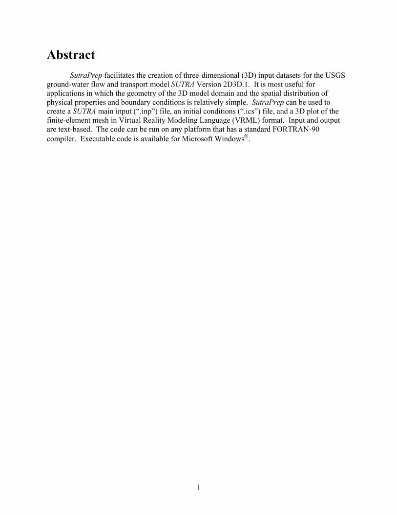
Abstract

SutraPrep facilitates the creation of three-dimensional (3D) input datasets for the USGS ground-water flow and transport model SUTRA Version 2D3D.1. It is most useful for applications in which the geometry of the 3D model domain and the spatial distribution of physical properties and boundary conditions is relatively simple. SutraPrep can be used to create a SUTRA main input (“.inp”) file, an initial conditions (“.ics”) file, and a 3D plot of the finite-element mesh in Virtual Reality Modeling Language (VRML) format. Input and output are text-based. The code can be run on any platform that has a standard FORTRAN-90 compiler. Executable code is available for Microsoft Windows.

1

Introduction

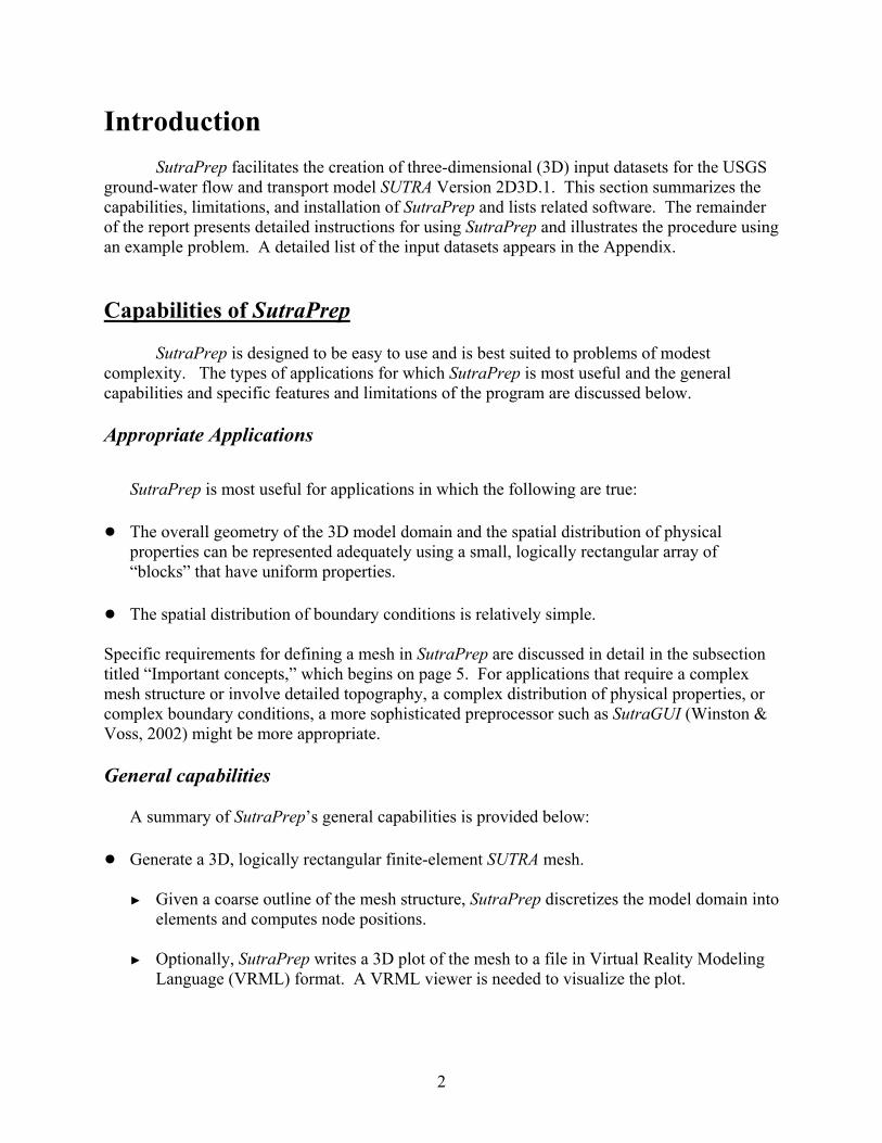
SutraPrep facilitates the creation of three-dimensional (3D) input datasets for the USGS ground-water flow and transport model SUTRA Version 2D3D.1. This section summarizes the capabilities, limitations, and installation of SutraPrep and lists related software. The remainder of the report presents detailed instructions for using SutraPrep and illustrates the procedure using an example problem. A detailed list of the input datasets appears in the Appendix. Capabilities of SutraPrep SutraPrep is designed to be easy to use and is best suited to problems of modest complexity. The types of applications for which SutraPrep is most useful and the general capabilities and specific features and limitations of the program are discussed below. Appropriate Applications

SutraPrep is most useful for applications in which the following are true: ●

●

●

The overall geometry of the 3D model domain and the spatial distribution of physical properties can be represented adequately using a small, logically rectangular array of “blocks” that have uniform properties.

The spatial distribution of boundary conditions is relatively simple.

Specific requirements for defining a mesh in SutraPrep are discussed in detail in the subsection titled “Important concepts,” which begins on page 5. For applications that require a complex mesh structure or involve detailed topography, a complex distribution of physical properties, or complex boundary conditions, a more sophisticated preprocessor such as SutraGUI (Winston & Voss, 2002) might be more appropriate. General capabilities

A summary of SutraPrep’s general capabilities is provided below:

Generate a 3D, logically rectangular finite-element SUTRA mesh.

► Given a coarse outline of the mesh structure, SutraPrep discretizes the model domain into elements and computes node positions.

► Optionally, SutraPrep writes a 3D plot of the mesh to a file in Virtual Reality Modeling

Language (VRML) format. A VRML viewer is needed to visualize the plot.

2

●

●

●

●

●

Create a SUTRA main input (“.inp”) file, with mesh-related data automatically filled in.

Create a SUTRA initial conditions (".ics") file.

Specific features and limitations

A summary of specific features and limitations of SutraPrep is provided below:

It is designed specifically for use with SUTRA Version 2D3D.1.

It can be run in Microsoft Windows or on any computing platform that has a standard FORTRAN-90 compiler.

Input and output are text-based.

Installation of SutraPrep

Installation of SutraPrep involves downloading the code and (for non-Windows platforms) compiling the source code. Details are provided below. Windows executable code

Executable code is available for Microsoft Windows 95/98/NT/2000. To install, download it from the USGS web site http://water.usgs.gov/nrp/gwsoftware to a Windows-based PC and uncompress it if necessary. FORTRAN source code

The FORTRAN source code is also available. It is contained in the source file "sprep.f". To install, download the source file from the USGS web site http://water.usgs.gov/nrp/gwsoftware, uncompress it if necessary, and compile it using a FORTRAN-90 compiler. Related software In addition to the SutraPrep code, other software might be required, depending on the output desired and the computing platform on which SutraPrep is to be installed.

3

VRML viewer

To display VRML plots of the finite-element mesh, a viewer that accepts VRML 2.0 is required. A number of such viewers are available, either as stand-alone applications or as plug-ins for web browsers. For example, CosmoPlayer is a viewer that works with the Netscape Navigator and Microsoft Internet Explorer web browsers. Some viewers can be downloaded free of charge over the Internet. FORTRAN-90 compiler

To install SutraPrep on a platform other than a Windows-based PC, or to make changes to the SutraPrep code, a standard FORTRAN-90 compiler is required.

4

Instructions for Using SutraPrep

This section provides detailed instructions for setting up a SUTRA problem using SutraPrep. First, the general procedure for using SutraPrep is outlined, and a number of important concepts related to the use of SutraPrep are discussed. Then, the types of output available and the input data requirements are described. The discussion ends with information regarding visualization of mesh plots and editing of the SUTRA “.inp” file. General procedure

The general procedure for using SutraPrep is summarized below: 1. Define the problem and decide how it will be discretized. 2. Create the SutraPrep input file. (The standard filename extension is “.prp”.) 3. Run SutraPrep and enter the name of the input (“.prp”) file. 4. If a VRML plot of the finite element mesh has been created, display it using a VRML

viewer. 5. If a SUTRA main input (“.inp”) file has been created, modify it (if necessary) before using the

file in a SUTRA run. Important concepts To use SutraPrep effectively, the user must be familiar with a number of concepts related to the definition of the coordinate system and the discretization of the physical problem. These concepts are discussed below. Right-handed coordinates

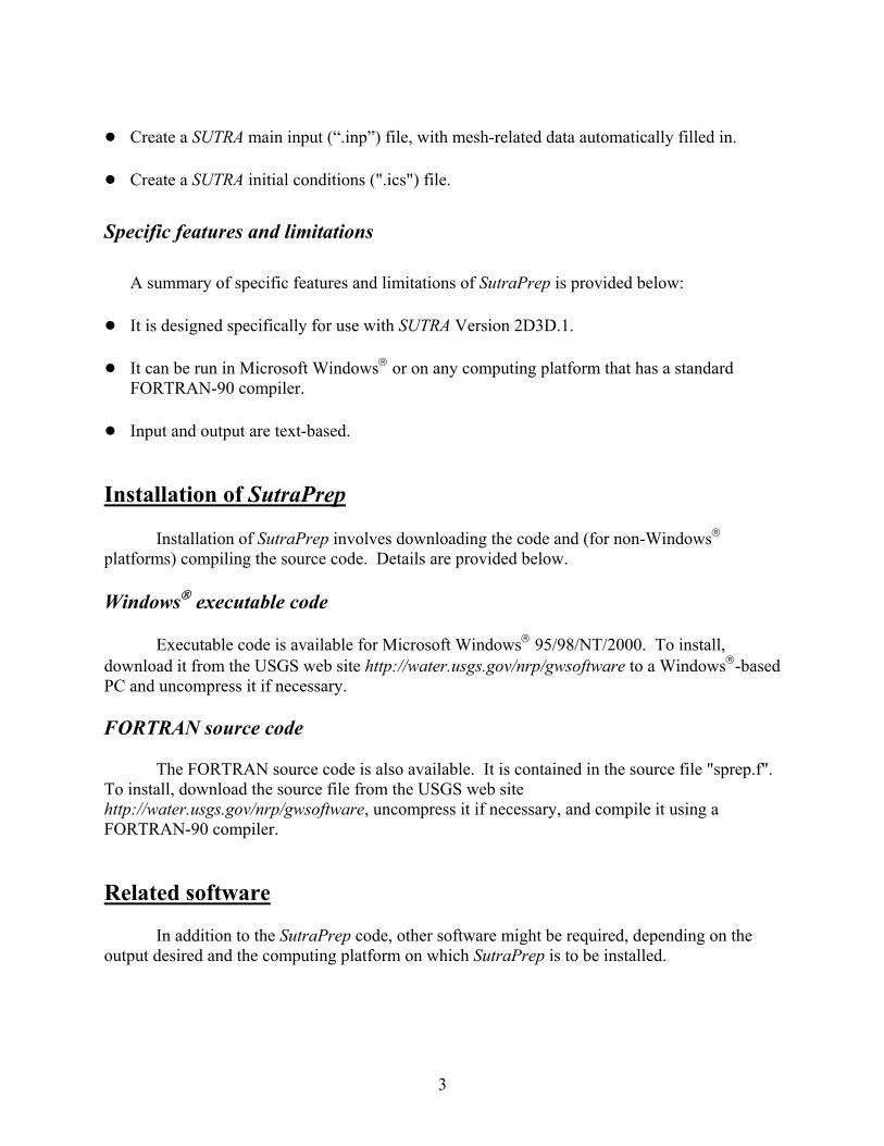
Like SUTRA, SutraPrep assumes a “right-handed” Cartesian coordinate system. Coordinate systems in which the positive x-, y-, and z-axes are related to each other as in figure 1a are called “right-handed.” Coordinate systems in which the positive x-, y-, and z-axes are related to each other as in figure 1b are called “left-handed.” The “handedness” of a coordinate system is unaffected by rotations or translations in space. However, note that a left-handed coordinate system can be made right-handed by reversing the direction of any one of the three axes, or of all three axes simultaneously. A right-handed (x, y, z) coordinate system must be used in the formulation of a SUTRA problem.

Confusion sometimes arises in the definition of the z-coordinate. Suppose the positive x- and y-axes are oriented in the horizontal plane, in the manner shown in figure 1a. If z represents

5

“elevation,” then the positive z-axis points upward, and the right-handed coordinate system shown in figure 1a is obtained. On the other hand, if z represents “depth,” then the positive z-axis points downward, and (apart from a rotation) the left-handed coordinate system shown in figure 1b is obtained. Should the user wish to work in terms of depth (that is, with the positive z-axis pointing downward), the direction of either the x-axis or the y-axis (but not both) must be reversed relative to its orientation in figure 1a, so that the coordinate system remains right-handed.

(a) (b)

Figure 1. Right-handed (a) and left-handed (b) Cartesian coordinate systems. All coordinate systems used with SutraPrep and SUTRA must be right-handed.

SUTRA elements and nodes

A SUTRA model consists of a collection of finite elements that share faces and corners. The corners of the elements are called nodes. Each three-dimensional SUTRA element is a generalized hexahedron: it has 12 straight edges that meet at 8 nodes and delineate 6 (possibly curved) faces. In SUTRA, porosity is specified nodewise, as are node coordinates; permeabilities and dispersivities are specified elementwise. For a model of any significant size, specifying information for all the nodes and elements individually requires either extraordinary patience or a special-purpose computer program. SutraPrep can make this process much less onerous by allowing the user to specify the geometry and physical properties for groupings (blocks) of elements.

6

SutraPrep blocks and corners

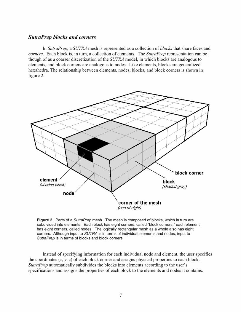
In SutraPrep, a SUTRA mesh is represented as a collection of blocks that share faces and corners. Each block is, in turn, a collection of elements. The SutraPrep representation can be though of as a coarser discretization of the SUTRA model, in which blocks are analogous to elements, and block corners are analogous to nodes. Like elements, blocks are generalized hexahedra. The relationship between elements, nodes, blocks, and block corners is shown in figure 2.

Figure 2. Parts of a SutraPrep mesh. The mesh is composed of blocks, which in turn are subdivided into elements. Each block has eight corners, called “block corners;” each element has eight corners, called nodes. The logically rectangular mesh as a whole also has eight corners. Although input to SUTRA is in terms of individual elements and nodes, input to SutraPrep is in terms of blocks and block corners.

Instead of specifying information for each individual node and element, the user specifies the coordinates (x, y, z) of each block corner and assigns physical properties to each block. SutraPrep automatically subdivides the blocks into elements according to the user’s specifications and assigns the properties of each block to the elements and nodes it contains.

7

Logically rectangular arrays

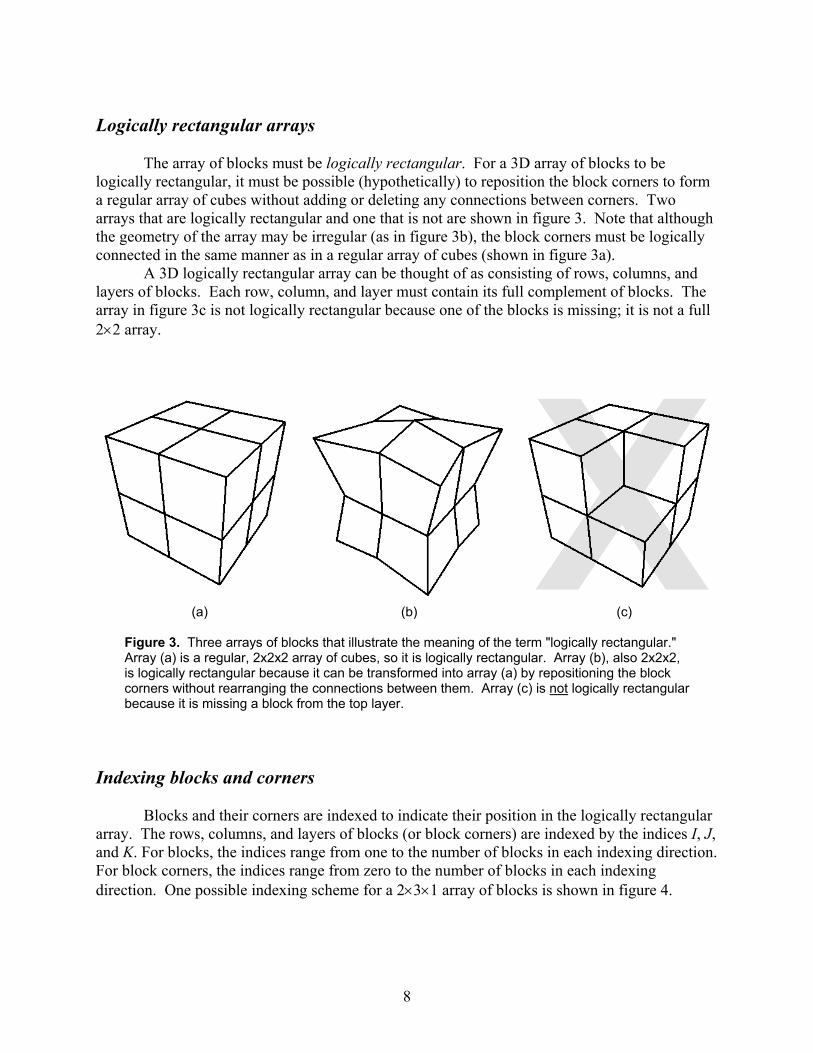
The array of blocks must be logically rectangular. For a 3D array of blocks to be logically rectangular, it must be possible (hypothetically) to reposition the block corners to form a regular array of cubes without adding or deleting any connections between corners. Two arrays that are logically rectangular and one that is not are shown in figure 3. Note that although the geometry of the array may be irregular (as in figure 3b), the block corners must be logically connected in the same manner as in a regular array of cubes (shown in figure 3a).

A 3D logically rectangular array can be thought of as consisting of rows, columns, and layers of blocks. Each row, column, and layer must contain its full complement of blocks. The array in figure 3c is not logically rectangular because one of the blocks is missing; it is not a full 2×2 array.

(a) (b) (c)

Figure 3. Three arrays of blocks that illustrate the meaning of the term "logically rectangular." Array (a) is a regular, 2x2x2 array of cubes, so it is logically rectangular. Array (b), also 2x2x2, is logically rectangular because it can be transformed into array (a) by repositioning the block corners without rearranging the connections between them. Array (c) is not logically rectangular because it is missing a block from the top layer.

Indexing blocks and corners

Blocks and their corners are indexed to indicate their position in the logically rectangular array. The rows, columns, and layers of blocks (or block corners) are indexed by the indices I, J, and K. For blocks, the indices range from one to the number of blocks in each indexing direction. For block corners, the indices range from zero to the number of blocks in each indexing direction. One possible indexing scheme for a 2×3×1 array of blocks is shown in figure 4.

8

Figure 4. A 2×3×1-block example that illustrates one possible choice of I, J, and K indexing directions.

The user designates one of the eight corners of the mesh as block corner (0, 0, 0). Block (1, 1, 1) is then the block that contains corner (0, 0, 0). The user also chooses the I, J, and K indexing directions. Any indexing direction can correspond to I, J, or K, subject to the restriction that the (I, J, K) indexing scheme must be right-handed (in the same sense that the (x, y, z) coordinate system must be right-handed; see figure 1a). In all, there are 8×3=24 possible right-handed indexing schemes for a given array of blocks. The user is free to choose whichever scheme is most convenient for the particular problem. The three schemes that are possible for one particular placement of block corner (0, 0, 0) are shown in figure 5. Numbering nodes

Node numbering can begin at any of the eight corners of the mesh. It proceeds node-by-node in any of one the three indexing directions, until a complete “row” of nodes is numbered; then row-after-row in either of the two remaining directions, until a complete “sheet” of nodes is numbered; and then sheet-after-sheet in the last remaining direction, until all the nodes are numbered.

9

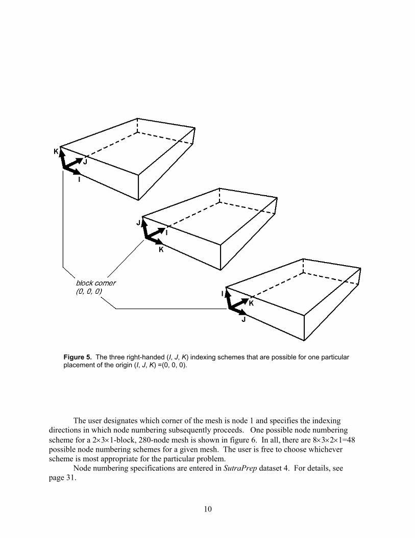
Figure 5. The three right-handed (I, J, K) indexing schemes that are possible for one particular placement of the origin (I, J, K) =(0, 0, 0).

The user designates which corner of the mesh is node 1 and specifies the indexing directions in which node numbering subsequently proceeds. One possible node numbering scheme for a 2×3×1-block, 280-node mesh is shown in figure 6. In all, there are 8×3×2×1=48 possible node numbering schemes for a given mesh. The user is free to choose whichever scheme is most appropriate for the particular problem.

Node numbering specifications are entered in SutraPrep dataset 4. For details, see page 31.

10

Figure 6. A 280-node example that illustrates one of the 48 possible node orderings. In this example, node numbering begins at the corner of the mesh that corresponds to (I, J, K)=(Imax, 0, Kmax), where the subscript “max” indicates the maximum value of an index. It proceeds first along the K-direction, then along the J-direction, and finally along the I-direction. Node numbers are shown for the first three “sheets” of nodes and for the visible corners of the mesh.

11

Specifying boundary conditions

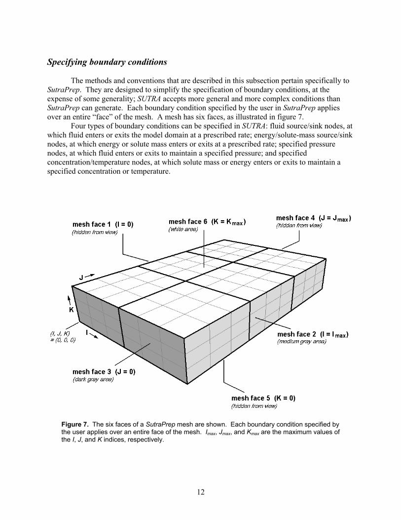
The methods and conventions that are described in this subsection pertain specifically to SutraPrep. They are designed to simplify the specification of boundary conditions, at the expense of some generality; SUTRA accepts more general and more complex conditions than SutraPrep can generate. Each boundary condition specified by the user in SutraPrep applies over an entire “face” of the mesh. A mesh has six faces, as illustrated in figure 7.

Four types of boundary conditions can be specified in SUTRA: fluid source/sink nodes, at which fluid enters or exits the model domain at a prescribed rate; energy/solute-mass source/sink nodes, at which energy or solute mass enters or exits at a prescribed rate; specified pressure nodes, at which fluid enters or exits to maintain a specified pressure; and specified concentration/temperature nodes, at which solute mass or energy enters or exits to maintain a specified concentration or temperature.

Figure 7. The six faces of a SutraPrep mesh are shown. Each boundary condition specified by the user applies over an entire face of the mesh. Imax, Jmax, and Kmax are the maximum values of the I, J, and K indices, respectively.

12

SutraPrep allows the user to specify each of these four types of boundary conditions.

However, only one boundary condition of each type may be specified on any given face of the mesh. At nodes that are shared by two or three faces to which the user has assigned the same type of boundary condition (but perhaps different values), the assignment that appears last in the SutraPrep input file prevails. For example, faces 2, 3, and 6 share a corner node. If a fluid source is assigned first to face 3, then to face 6, and then to face 2, then the corner node will inherit the value assigned to face 2.

Sources of fluid, energy, and solute mass are specified in SutraPrep on a per area basis. The amount of source apportioned by SutraPrep to a given node is proportional to the area associated with that node. The method SutraPrep uses to compute the area associated with a node is shown in figure 8.

Figure 8. Method used by SutraPrep to compute the areas associated with nodes. Shown is a patch of 9 nodes (black circles) on a curved face of the mesh. The area associated with the center node is shaded medium gray. It is computed as the sum of the areas of the 8 triangles formed by connecting the center node, the 4 midpoints between nodes (open circles), and the 4 centroids of the element faces (dark gray circles) as shown in the figure. Areas are computed similarly for nodes at an edge or corner of the mesh, except that fewer triangles contribute to the total area (four for a node on an edge of the mesh; two for a node at a corner of the mesh). Solid lines represent connections between nodes (i.e., element edges); dashed lines represent additional connections used to form the triangles.

Specified concentrations or temperatures in SutraPrep are uniform over each face of the mesh. Specified pressures may vary linearly in space. The user specifies a linear pressure field by assigning the pressure at a reference point and specifying the x-, y- and z-components of the uniform pressure gradient. The pressure assigned by SutraPrep to each node on the face is the value of the specified pressure field at the node. This procedure makes it easy to specify a uniform pressure, or hydrostatic pressures that correspond to a uniform fluid density.

Boundary condition specifications are entered in SutraPrep dataset 6. For details, see page 37.

13

Specifying initial conditions

The initial concentration is given a user-specified uniform value throughout the mesh in SutraPrep. The initial pressures may vary linearly in space. The user specifies a linear initial pressure field by assigning the pressure at a reference point and specifying the x-, y- and z-components of the uniform pressure gradient. The initial pressure assigned by SutraPrep to each node on the face is the value of the initial pressure field at the node. This procedure makes it easy to specify a uniform initial pressure, or hydrostatic initial pressures that correspond to a uniform fluid density.

Initial conditions are entered in SutraPrep dataset 7. For details, see page 41. Types of output available

During each run, SutraPrep automatically creates a user-named log file that contains a summary of the run. The user may request up to three additional types of output, each corresponding to a separate output file. The output files available are described below. Log (“.prl”) file

The log file summarizes the SutraPrep run and is generated automatically during every run. The recommended file extension for this user-named file is “.prl”.

Depending on the additional types of output requested by the user, the log file may include any of the following:

► a list of filenames ► a summary of the discretization ► a description of the node numbering scheme ► a list of minimum and maximum values of the node coordinates ► a list of minimum and maximum values of the nodewise and elementwise physical properties ► a summary of boundary conditions ► a description of the initial conditions ► VRML mesh plot information SUTRA “.inp” file

SutraPrep can create a SUTRA ".inp" (main input) file with all mesh-related data (mesh dimensions; nodewise and elementwise data; boundary condition information, if any; and the element incidence list) automatically filled in. For all remaining information, SutraPrep can either insert placeholders or import actual values from SUTRA datasets 1 - 13 of an existing ".inp" file. Boundary conditions generated by SutraPrep apply to entire faces of the logically rectangular mesh; any boundary conditions that do not apply to an entire face must be generated separately by the user. For details about specifying boundary conditions, see “Specifying boundary conditions” on page 12.

14

SUTRA “.ics” file

SutraPrep can generate a complete SUTRA initial conditions file. For details about specifying initial conditions, see “Specifying initial conditions” on page 14. Mesh plot in VRML

SutraPrep can generate a text file that contains a representation of the 3D finite-element mesh in VRML 2.0 format.

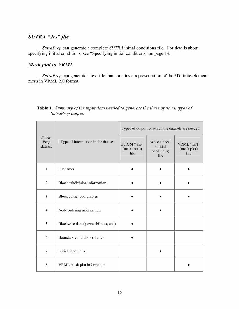
Table 1. Summary of the input data needed to generate the three optional types of SutraPrep output.

Types of output for which the datasets are needed

Sutra-Prep

dataset Type of information in the dataset

SUTRA ".inp" (main input)

file

SUTRA ".ics"

(initial conditions)

file

VRML ".wrl" (mesh plot)

file

1

Filenames ● ● ●

2

Block subdivision information ● ● ●

3

Block corner coordinates ● ● ●

4

Node ordering information ● ●

5

Blockwise data (permeabilities, etc.) ●

6

Boundary conditions (if any) ●

7

Initial conditions ●

8

VRML mesh plot information ●

15

Input data requirements

SutraPrep input data are organized into eight datasets. Each dataset contains one or more items of data that relate to a particular aspect of the model description or the output specifications. The user enters the datasets into a single input file. The input filename customarily ends with the extension “.prp”. Depending on the types of SutraPrep output desired, certain datasets may be omitted from the input file (table 1).

The SutraPrep datasets are described briefly below. For a detailed description, see the Appendix, which begins on page 26. DATASET 1: Filenames

Dataset 1 is a list of up to four filenames. The first three are the names of SutraPrep output files. The fourth is the name of an existing “.inp” file from which SUTRA data are to be imported. Data are imported only from SUTRA datasets 1 – 13 of the existing “.inp” file. DATASET 2: Block subdivision information

Dataset 2 specifies the number of blocks into which the model is divided and the number of elements into which the blocks are subdivided. DATASET 3: Block corner coordinates

Dataset 3 lists the coordinates (x, y, z) of the block corners. DATASET 4: Node ordering information

Dataset 4 specifies the location of node 1 and the order in which the nodes are to be numbered. DATASET 5: Blockwise data

Dataset 5 is a block-by-block listing of porosities, permeabilities, and dispersivities. DATASET 6: Boundary conditions

Dataset 6 is a listing of boundary conditions. Each boundary condition applies to an entire face of the logically rectangular mesh; any boundary conditions that do not apply to an entire face must be generated separately by the user. A boundary condition specification consists of the boundary condition type and the face to which it applies, followed by any relevant parameters. Sources of fluid, energy, or solute mass are specified as uniform values per unit area. Specified pressures may vary linearly in space. Specified concentrations/temperatures are uniform.

16

DATASET 7: Initial conditions

Dataset 7 is a listing of the initial time, pressures, and concentrations or temperatures. Initial pressures may be uniform or may vary linearly in space. Initial concentrations or temperatures are uniform. DATASET 8: VRML mesh plot information

Dataset 8 specifies what is to be plotted (element and block edges, or only block edges) and the scaling to be applied to the plot in the x-, y- and z-directions.

Viewing the finite-element mesh

Any viewer that accepts VRML 2.0 can be used to display 3D mesh plots created by SutraPrep. A number of such viewers are available, either as stand-alone applications or as plug-ins for web browsers. For example, CosmoPlayer is a viewer that works with the Netscape Navigator and Microsoft Internet Explorer web browsers. Certain versions of some viewers can be downloaded free of charge over the Internet.

When the image of the mesh is first loaded into the viewer, is it viewed looking down the positive z-axis toward the origin. The viewer’s controls can be used to change the perspective. Visual inspection of the mesh from a variety of angles can make it easier to verify that the mesh is indeed structured as intended. For the user’s convenience, SutraPrep generates three preprogrammed viewpoints (looking along the x-, y-, and z- axes), which are supported by some VRML viewers and provide an easy mechanism for switching between views.

If the image on the screen cannot be printed directly from the viewer, it might be possible to use “screen capture” to create a bitmap of the image. For example, in Windows NT, one could press SHIFT-PrintScreen to copy the contents of the screen, then open the Paint utility (in the “Accessories” group) and press CTRL-V to paste in the copied image. The image could then be edited, printed, or saved as a bitmap that could be imported as a graphic into another application, such as a word processor. This method was used to create many of the figures in this report. Editing the SUTRA “.inp” (main input) file

Practically any text editor can be used to edit SUTRA input files created by SutraPrep. SutraPrep automatically fills in any mesh-related data, including mesh dimensions, nodewise and elementwise data, and the element incidence list. For each data item it does not compute or import, SutraPrep inserts a placeholder. For example, it writes the placeholder “[ITMAX]” at the beginning of the line devoted to SUTRA dataset 6. The user must insert (or import) actual values for all required data before using the input file in a SUTRA run.

17

Example Problem

The example problem described in this section illustrates the process of setting up a SUTRA problem using SutraPrep. Problem description

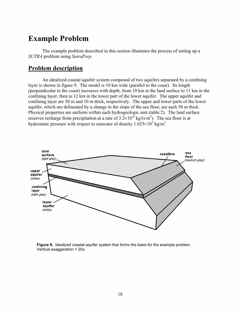
An idealized coastal aquifer system composed of two aquifers separated by a confining layer is shown in figure 9. The model is 10 km wide (parallel to the coast). Its length (perpendicular to the coast) increases with depth, from 10 km at the land surface to 11 km in the confining layer, then to 12 km in the lower part of the lower aquifer. The upper aquifer and confining layer are 50 m and 10 m thick, respectively. The upper and lower parts of the lower aquifer, which are delineated by a change in the slope of the sea floor, are each 50 m thick. Physical properties are uniform within each hydrogeologic unit (table 2). The land surface receives recharge from precipitation at a rate of 3.2×10-6 kg/(s·m2). The sea floor is at hydrostatic pressure with respect to seawater of density 1.025×103 kg/m3.

Figure 9. Idealized coastal aquifer system that forms the basis for the example problem. Vertical exaggeration = 20x.

18

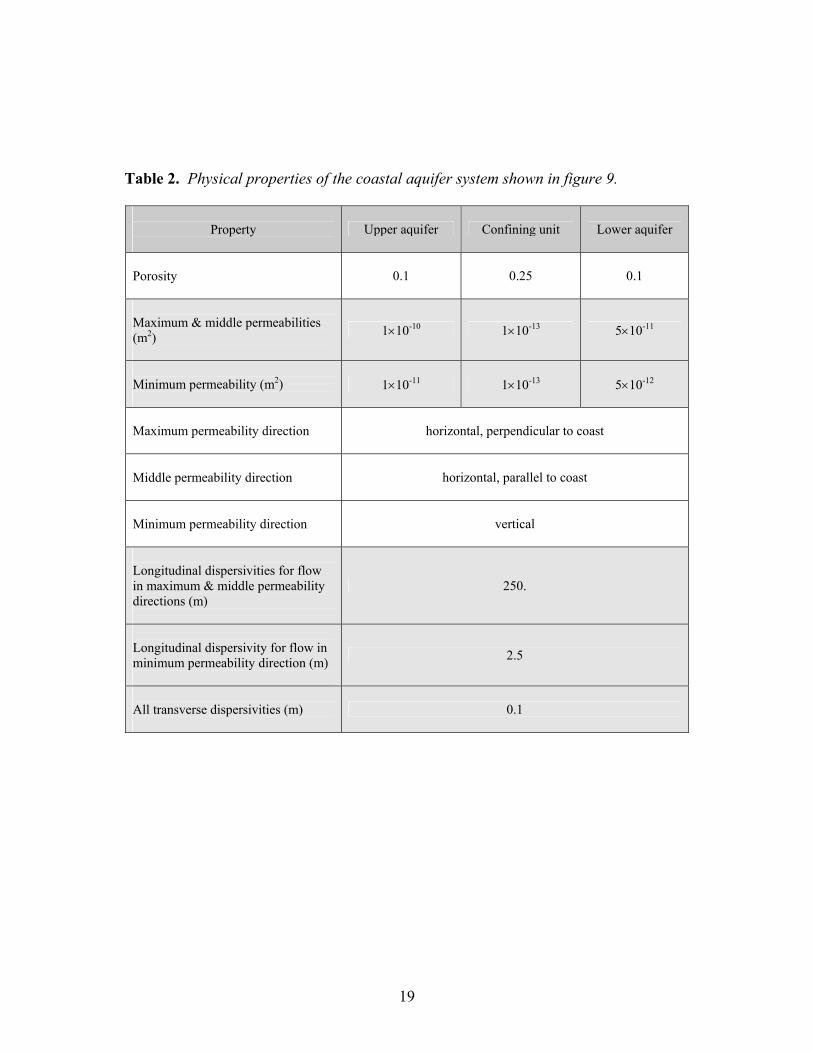
Table 2. Physical properties of the coastal aquifer system shown in figure 9.

Property

Upper aquifer Confining unit Lower aquifer

Porosity

0.1 0.25 0.1

Maximum & middle permeabilities (m2)

1×10-10 1×10-13 5×10-11

Minimum permeability (m2)

1×10-11 1×10-13 5×10-12

Maximum permeability direction

horizontal, perpendicular to coast

Middle permeability direction

horizontal, parallel to coast

Minimum permeability direction

vertical

Longitudinal dispersivities for flow in maximum & middle permeability directions (m)

250.

Longitudinal dispersivity for flow in minimum permeability direction (m)

2.5

All transverse dispersivities (m)

0.1

19

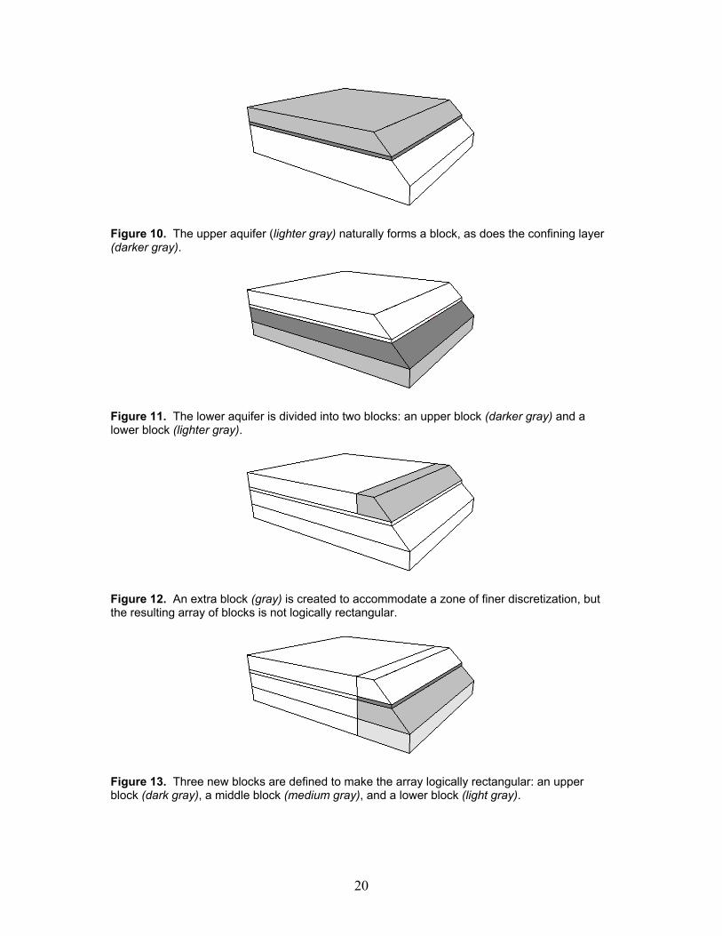
Figure 10. The upper aquifer (lighter gray) naturally forms a block, as does the confining layer (darker gray).

Figure 11. The lower aquifer is divided into two blocks: an upper block (darker gray) and a lower block (lighter gray).

Figure 12. An extra block (gray) is created to accommodate a zone of finer discretization, but the resulting array of blocks is not logically rectangular.

Figure 13. Three new blocks are defined to make the array logically rectangular: an upper block (dark gray), a middle block (medium gray), and a lower block (light gray).

20

Division of the model domain into blocks

This example problem illustrates four reasons for dividing a model domain into two or more blocks: 1) Regions with different physical properties. The upper and lower aquifers and the confining

layer each have different physical properties. Because of their hexahedral shape, the upper aquifer and the confining layer naturally form blocks (figure 10). The lower aquifer does not.

2) Blocks must be generalized hexahedra. Because the slope of the sea floor changes within the

lower aquifer, the lower aquifer has 10 corners (points where straight edges meet) and must be divided into at least two blocks. The lower aquifer is shown divided into two blocks by a horizontal, rectangular face in figure 11.

3) Regions with different fineness of discretization. Suppose a zone of finer mesh spacing is

desired in the upper aquifer, near the sea. An extra block in which a different discretization can be specified is shown in figure 12.

4) The array of blocks must be logically rectangular. The array of blocks shown in figure 12 is

invalid because the top layer of blocks (the upper aquifer) consists of two blocks, and the underlying layers of blocks each comprise a single block. To correct this, the division of layers into two blocks must be continued down through the entire model domain. The result is a 2×1×4 array of blocks (figure 13).

Subdivision into nodes and elements

The model domain is shown subdivided into nodes and elements in figure 14. The node numbering scheme depicted is one of 48 possibilities. SutraPrep input file for example problem

A SutraPrep input file that corresponds to the coastal aquifer system example problem is shown in table 3. The datasets are described below. ●

●

DATASET 1: SutraPrep is to create a SUTRA main input file called ‘coastal.inp’, an initial conditions file called ‘coastal.ics’, and a VRML mesh plot called ‘coastal.wrl’. No data are to be imported from an existing ‘.inp’ file; data items not written by SutraPrep will be entered manually. A summary of the SutraPrep run will be written to file ‘coastal.prl’.

DATASET 2: The model consists of a 2×1×4 array of blocks. The two blocks along the I-direction are subdivided into 18 and 6 elements, respectively. The single block along the J-

21

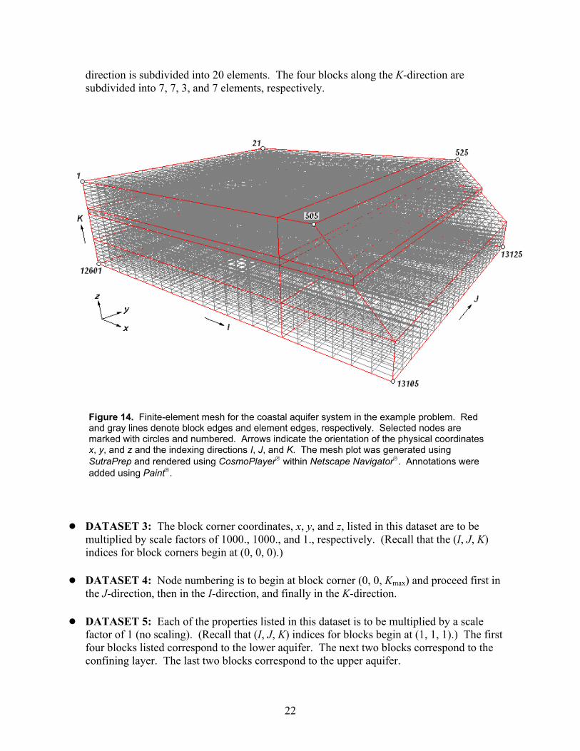
direction is subdivided into 20 elements. The four blocks along the K-direction are subdivided into 7, 7, 3, and 7 elements, respectively.

Figure 14. Finite-element mesh for the coastal aquifer system in the example problem. Red and gray lines denote block edges and element edges, respectively. Selected nodes are marked with circles and numbered. Arrows indicate the orientation of the physical coordinates x, y, and z and the indexing directions I, J, and K. The mesh plot was generated using SutraPrep and rendered using CosmoPlayer within Netscape Navigator. Annotations were added using Paint.

●

●

●

DATASET 3: The block corner coordinates, x, y, and z, listed in this dataset are to be multiplied by scale factors of 1000., 1000., and 1., respectively. (Recall that the (I, J, K) indices for block corners begin at (0, 0, 0).) DATASET 4: Node numbering is to begin at block corner (0, 0, Kmax) and proceed first in the J-direction, then in the I-direction, and finally in the K-direction.

DATASET 5: Each of the properties listed in this dataset is to be multiplied by a scale factor of 1 (no scaling). (Recall that (I, J, K) indices for blocks begin at (1, 1, 1).) The first four blocks listed correspond to the lower aquifer. The next two blocks correspond to the confining layer. The last two blocks correspond to the upper aquifer.

22

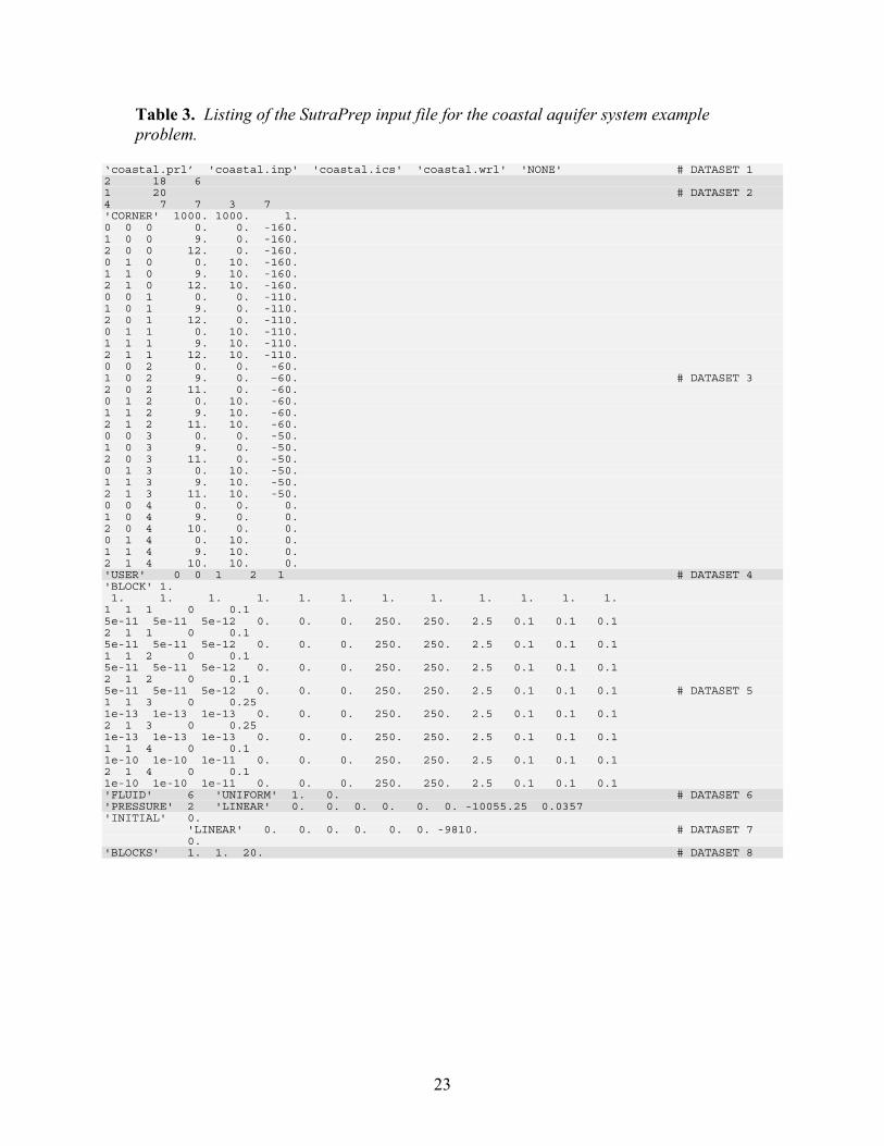
Table 3. Listing of the SutraPrep input file for the coastal aquifer system example problem.

‘coastal.prl’ 'coastal.inp' 'coastal.ics' 'coastal.wrl' 'NONE' # DATASET 1 2 18 6 1 20 # DATASET 2 4 7 7 3 7 'CORNER' 1000. 1000. 1. 0 0 0 0. 0. -160. 1 0 0 9. 0. -160. 2 0 0 12. 0. -160. 0 1 0 0. 10. -160. 1 1 0 9. 10. -160. 2 1 0 12. 10. -160. 0 0 1 0. 0. -110. 1 0 1 9. 0. -110. 2 0 1 12. 0. -110. 0 1 1 0. 10. -110. 1 1 1 9. 10. -110. 2 1 1 12. 10. -110. 0 0 2 0. 0. -60. 1 0 2 9. 0. –60. # DATASET 3 2 0 2 11. 0. -60. 0 1 2 0. 10. -60. 1 1 2 9. 10. -60. 2 1 2 11. 10. -60. 0 0 3 0. 0. -50. 1 0 3 9. 0. -50. 2 0 3 11. 0. -50. 0 1 3 0. 10. -50. 1 1 3 9. 10. -50. 2 1 3 11. 10. -50. 0 0 4 0. 0. 0. 1 0 4 9. 0. 0. 2 0 4 10. 0. 0. 0 1 4 0. 10. 0. 1 1 4 9. 10. 0. 2 1 4 10. 10. 0. 'USER' 0 0 1 2 1 # DATASET 4 'BLOCK' 1. 1. 1. 1. 1. 1. 1. 1. 1. 1. 1. 1. 1. 1 1 1 0 0.1 5e-11 5e-11 5e-12 0. 0. 0. 250. 250. 2.5 0.1 0.1 0.1 2 1 1 0 0.1 5e-11 5e-11 5e-12 0. 0. 0. 250. 250. 2.5 0.1 0.1 0.1 1 1 2 0 0.1 5e-11 5e-11 5e-12 0. 0. 0. 250. 250. 2.5 0.1 0.1 0.1 2 1 2 0 0.1 5e-11 5e-11 5e-12 0. 0. 0. 250. 250. 2.5 0.1 0.1 0.1 # DATASET 5 1 1 3 0 0.25 1e-13 1e-13 1e-13 0. 0. 0. 250. 250. 2.5 0.1 0.1 0.1 2 1 3 0 0.25 1e-13 1e-13 1e-13 0. 0. 0. 250. 250. 2.5 0.1 0.1 0.1 1 1 4 0 0.1 1e-10 1e-10 1e-11 0. 0. 0. 250. 250. 2.5 0.1 0.1 0.1 2 1 4 0 0.1 1e-10 1e-10 1e-11 0. 0. 0. 250. 250. 2.5 0.1 0.1 0.1 'FLUID' 6 'UNIFORM' 1. 0. # DATASET 6 'PRESSURE' 2 'LINEAR' 0. 0. 0. 0. 0. 0. -10055.25 0.0357 'INITIAL' 0. 'LINEAR' 0. 0. 0. 0. 0. 0. -9810. # DATASET 7 0. 'BLOCKS' 1. 1. 20. # DATASET 8

23

●

●

●

DATASET 6: A uniform fluid source, which represents natural recharge, is imposed on the land surface. A linearly varying pressure, which represents hydrostatic pressure for a column of seawater, is imposed along the sea floor.

DATASET 7: The initial pressure varies linearly with depth, which represents hydrostatic pressure for a column of fresh water. The initial solute concentration is zero throughout the model.

DATASET 8: The VRML mesh plot is to include only block edges and is to be drawn with a vertical exaggeration of 20×.

24

References Voss, C. I., and Provost, A. M., 2002, SUTRA - A model for saturated-unsaturated variable-

density ground-water flow with solute or energy transport, U.S. Geological Survey Water-Resources Investigations Report 02-4231, 250 p.

Winston, R.B. and Voss, C.I., 2003, SutraGUI, a graphical-user interface for SUTRA, a model

for ground-water flow with solute or energy transport: U.S. Geological Survey Open-File Report 03-285, 114 p.

25

Appendix: SutraPrep Input Data List Program Series: SutraPrep Program Version: 3D.1

SutraPrep reads the “.prp” input file in a list-directed manner. Input data appearing on the same line should be space- or tab-separated. Any data that are not optional must be given values in the input file (blanks are not sufficient). All input variables of “character” type should be enclosed in single quotation marks unless specified otherwise.

After SutraPrep has read all the parameters it needs from a given line, it ignores the rest of the line. Thus, a comment (or any text) can be appended to the end of any line of input data, provided all the required parameters have already been entered on that line. At least one space or tab must be left between the last required parameter and the beginning of a comment.

26

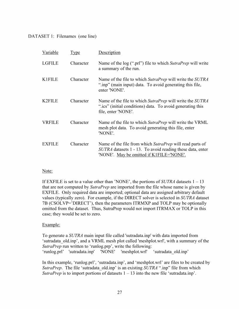
DATASET 1: Filenames (one line) Variable Type Description LGFILE Character Name of the log (“.prl”) file to which SutraPrep will write

a summary of the run. K1FILE Character Name of the file to which SutraPrep will write the SUTRA

“.inp” (main input) data. To avoid generating this file, enter 'NONE'.

K2FILE Character Name of the file to which SutraPrep will write the SUTRA

“.ics” (initial conditions) data. To avoid generating this file, enter 'NONE'.

VRFILE Character Name of the file to which SutraPrep will write the VRML

mesh plot data. To avoid generating this file, enter 'NONE'.

EXFILE Character Name of the file from which SutraPrep will read parts of

SUTRA datasets 1 - 13. To avoid reading these data, enter 'NONE'. May be omitted if K1FILE='NONE'.

Note: If EXFILE is set to a value other than ’NONE’, the portions of SUTRA datasets 1 – 13 that are not computed by SutraPrep are imported from the file whose name is given by EXFILE. Only required data are imported; optional data are assigned arbitrary default values (typically zero). For example, if the DIRECT solver is selected in SUTRA dataset 7B (CSOLVP=’DIRECT’), then the parameters ITRMXP and TOLP may be optionally omitted from the dataset. Thus, SutraPrep would not import ITRMAX or TOLP in this case; they would be set to zero. Example: To generate a SUTRA main input file called 'sutradata.inp' with data imported from ‘sutradata_old.inp’, and a VRML mesh plot called 'meshplot.wrl', with a summary of the SutraPrep run written to ‘runlog.prp’, write the following: ‘runlog.prl’ 'sutradata.inp' 'NONE' 'meshplot.wrl' ‘sutradata_old.inp’ In this example, ‘runlog.prl’, ‘sutradata.inp’, and ‘meshplot.wrl’ are files to be created by SutraPrep. The file ‘sutradata_old.inp’ is an existing SUTRA “.inp” file from which SutraPrep is to import portions of datasets 1 – 13 into the new file ‘sutradata.inp’.

27

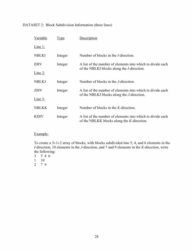
DATASET 2: Block Subdivision Information (three lines) Variable Type Description Line 1:

NBLKI Integer Number of blocks in the I-direction. IDIV Integer A list of the number of elements into which to divide each

of the NBLKI blocks along the I-direction. Line 2:

NBLKJ Integer Number of blocks in the J-direction. JDIV Integer A list of the number of elements into which to divide each

of the NBLKJ blocks along the J-direction. Line 3:

NBLKK Integer Number of blocks in the K-direction. KDIV Integer A list of the number of elements into which to divide each

of the NBLKK blocks along the K-direction.

Example: To create a 3×1×2 array of blocks, with blocks subdivided into 5, 4, and 6 elements in the I-direction, 10 elements in the J-direction, and 7 and 9 elements in the K-direction, write the following: 3 5 4 6 1 10 2 7 9

28

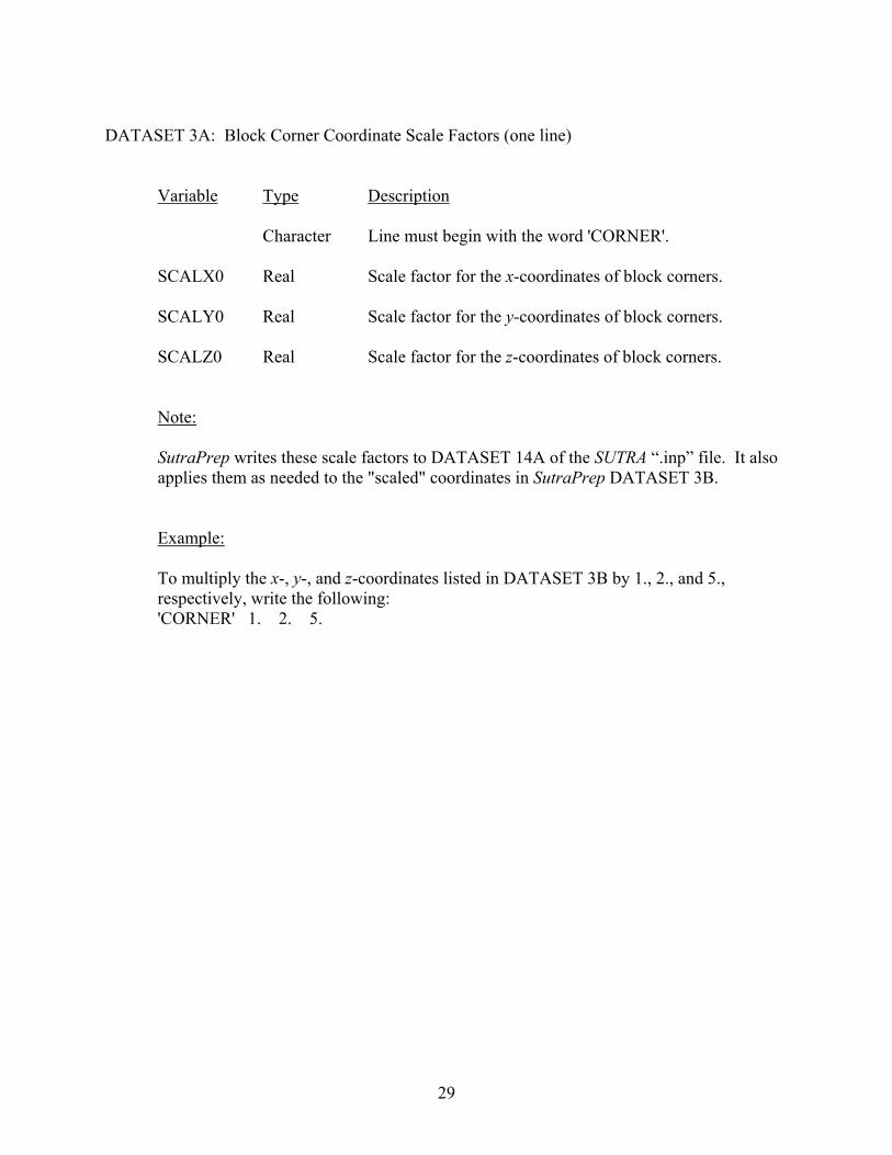
DATASET 3A: Block Corner Coordinate Scale Factors (one line) Variable Type Description Character Line must begin with the word 'CORNER'.

SCALX0 Real Scale factor for the x-coordinates of block corners.

SCALY0 Real Scale factor for the y-coordinates of block corners.

SCALZ0 Real Scale factor for the z-coordinates of block corners. Note:

SutraPrep writes these scale factors to DATASET 14A of the SUTRA “.inp” file. It also applies them as needed to the "scaled" coordinates in SutraPrep DATASET 3B.

Example: To multiply the x-, y-, and z-coordinates listed in DATASET 3B by 1., 2., and 5., respectively, write the following: 'CORNER' 1. 2. 5.

29

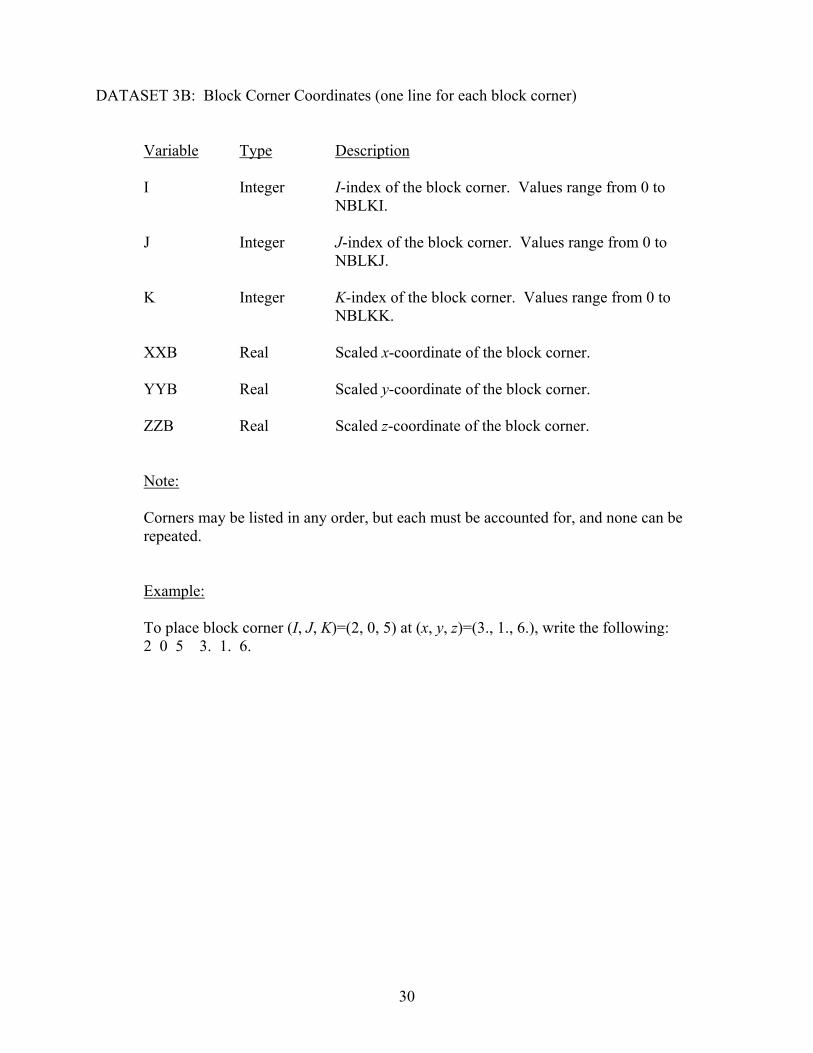
DATASET 3B: Block Corner Coordinates (one line for each block corner) Variable Type Description I Integer I-index of the block corner. Values range from 0 to

NBLKI. J Integer J-index of the block corner. Values range from 0 to

NBLKJ. K Integer K-index of the block corner. Values range from 0 to

NBLKK. XXB Real Scaled x-coordinate of the block corner. YYB Real Scaled y-coordinate of the block corner. ZZB Real Scaled z-coordinate of the block corner.

Note: Corners may be listed in any order, but each must be accounted for, and none can be repeated.

Example: To place block corner (I, J, K)=(2, 0, 5) at (x, y, z)=(3., 1., 6.), write the following: 2 0 5 3. 1. 6.

30

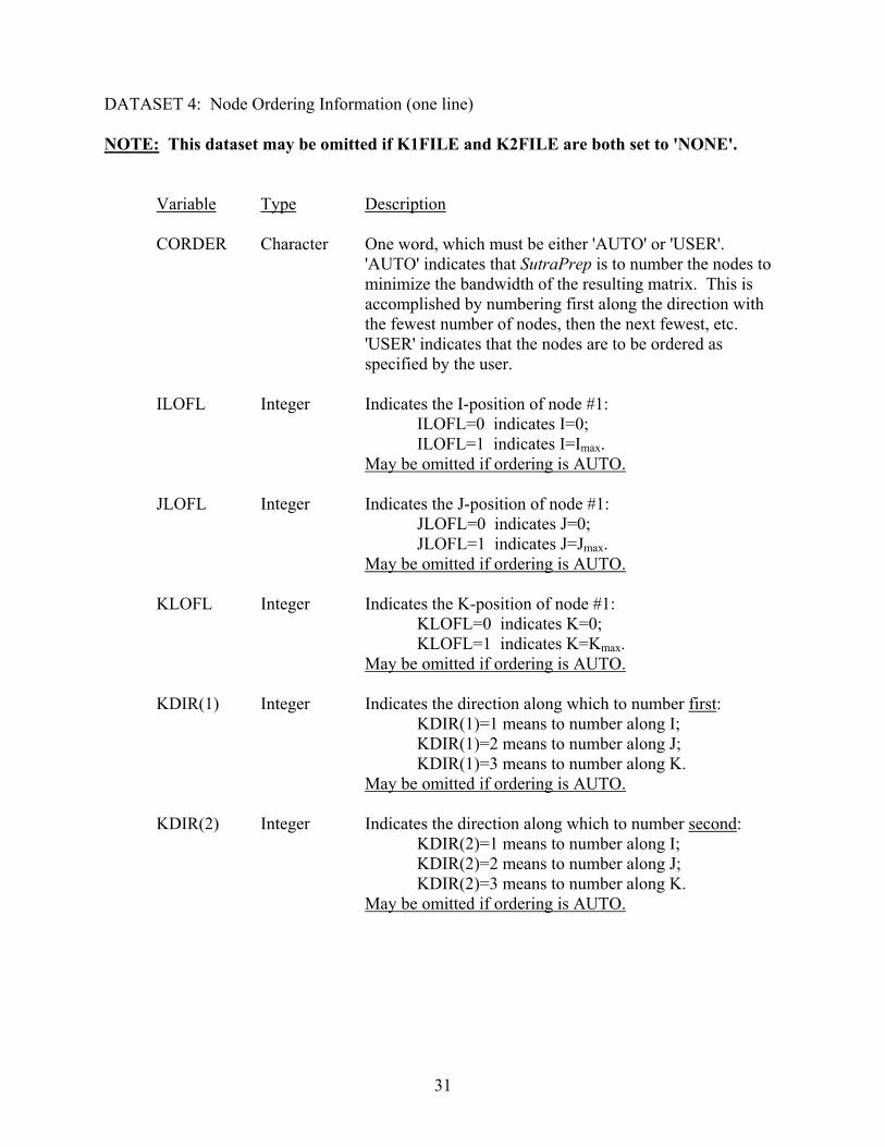
DATASET 4: Node Ordering Information (one line) NOTE: This dataset may be omitted if K1FILE and K2FILE are both set to 'NONE'. Variable Type Description CORDER Character One word, which must be either 'AUTO' or 'USER'.

'AUTO' indicates that SutraPrep is to number the nodes to minimize the bandwidth of the resulting matrix. This is accomplished by numbering first along the direction with the fewest number of nodes, then the next fewest, etc. 'USER' indicates that the nodes are to be ordered as specified by the user.

ILOFL Integer Indicates the I-position of node #1: ILOFL=0 indicates I=0; ILOFL=1 indicates I=Imax. May be omitted if ordering is AUTO. JLOFL Integer Indicates the J-position of node #1: JLOFL=0 indicates J=0; JLOFL=1 indicates J=Jmax. May be omitted if ordering is AUTO. KLOFL Integer Indicates the K-position of node #1: KLOFL=0 indicates K=0; KLOFL=1 indicates K=Kmax. May be omitted if ordering is AUTO. KDIR(1) Integer Indicates the direction along which to number first: KDIR(1)=1 means to number along I; KDIR(1)=2 means to number along J; KDIR(1)=3 means to number along K. May be omitted if ordering is AUTO. KDIR(2) Integer Indicates the direction along which to number second: KDIR(2)=1 means to number along I; KDIR(2)=2 means to number along J; KDIR(2)=3 means to number along K. May be omitted if ordering is AUTO.

31

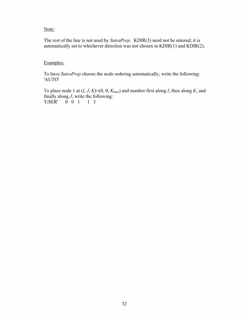
Note: The rest of the line is not used by SutraPrep. KDIR(3) need not be entered; it is automatically set to whichever direction was not chosen in KDIR(1) and KDIR(2). Examples:

To have SutraPrep choose the node ordering automatically, write the following: 'AUTO' To place node 1 at (I, J, K)=(0, 0, Kmax) and number first along I, then along K, and finally along J, write the following: 'USER' 0 0 1 1 3

32

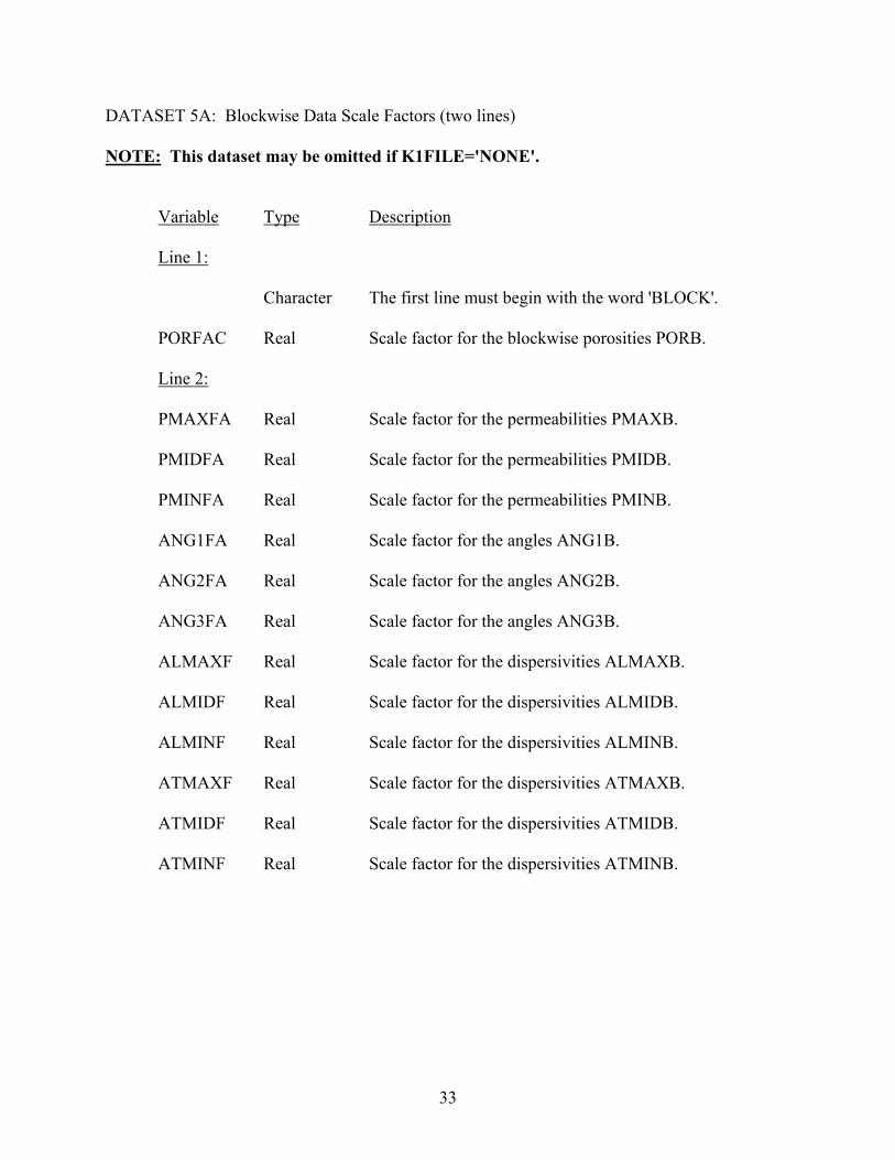
DATASET 5A: Blockwise Data Scale Factors (two lines) NOTE: This dataset may be omitted if K1FILE='NONE'. Variable Type Description Line 1: Character The first line must begin with the word 'BLOCK'. PORFAC Real Scale factor for the blockwise porosities PORB. Line 2: PMAXFA Real Scale factor for the permeabilities PMAXB. PMIDFA Real Scale factor for the permeabilities PMIDB. PMINFA Real Scale factor for the permeabilities PMINB. ANG1FA Real Scale factor for the angles ANG1B. ANG2FA Real Scale factor for the angles ANG2B. ANG3FA Real Scale factor for the angles ANG3B. ALMAXF Real Scale factor for the dispersivities ALMAXB. ALMIDF Real Scale factor for the dispersivities ALMIDB. ALMINF Real Scale factor for the dispersivities ALMINB. ATMAXF Real Scale factor for the dispersivities ATMAXB. ATMIDF Real Scale factor for the dispersivities ATMIDB. ATMINF Real Scale factor for the dispersivities ATMINB.

33

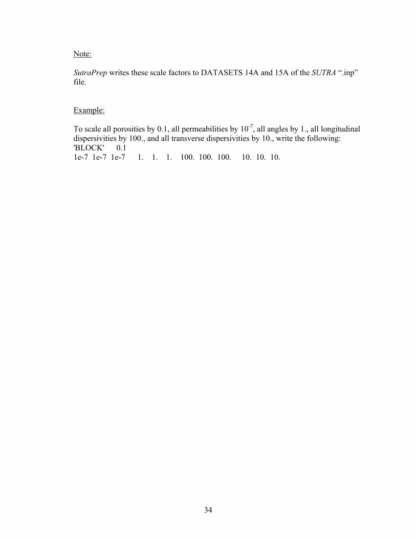
Note: SutraPrep writes these scale factors to DATASETS 14A and 15A of the SUTRA “.inp” file.

Example: To scale all porosities by 0.1, all permeabilities by 10-7, all angles by 1., all longitudinal dispersivities by 100., and all transverse dispersivities by 10., write the following: 'BLOCK' 0.1 1e-7 1e-7 1e-7 1. 1. 1. 100. 100. 100. 10. 10. 10.

34

DATASET 5B: Blockwise Data (two lines for each block) NOTE: This dataset may be omitted if K1FILE='NONE'. Variable Type Description Line 1: I Integer I-index of the block. Values range from 1 to NBLKI. J Integer J-index of the block. Values range from 1 to NBLKJ. K Integer K-index of the block. Values range from 1 to NBLKK. LREGB Integer Unsaturated flow property region number to which block

(I, J, K) belongs. A value must be entered even if the flow is saturated only.

PORB Real Scaled porosity of block (I, J, K). Line 2: PMAXB Real Scaled maximum permeability value of block (I, J, K). PMIDB Real Scaled middle permeability value of block (I, J, K). PMINB Real Scaled minimum permeability value of block (I, J, K). ANG1B Real Scaled angle within the x,y-plane, measured in degrees

counterclockwise from +x-direction to maximum permeability direction in block (I, J, K).

ANG2B Real Scaled angle measured (after ANG1B has been applied) in degrees upward from x,y-plane to maximum permeability direction in block (I, J, K).

ANG3B Real Scaled angle about the axis of maximum permeability,

measured (after ANG1B and ANG2B have been applied) in degrees, looking down the positive half of the axis toward the origin, and counterclockwise from the horizontal to the middle permeability direction in block (I, J, K).

ALMAXB Real Scaled longitudinal dispersivity value of block (I, J, K) in

the direction of maximum permeability PMAXB.

35

ALMIDB Real Scaled longitudinal dispersivity value of block (I, J, K) in the direction of middle permeability PMIDB.

ALMINB Real Scaled longitudinal dispersivity value of block (I, J, K) in

the direction of minimum permeability PMINB. ATMAXB Real Scaled transverse dispersivity value of block (I, J, K) in the

direction of maximum permeability PMAXB. ATMIDB Real Scaled transverse dispersivity value of block (I, J, K) in the

direction of middle permeability PMIDB. ATMINB Real Scaled transverse dispersivity value of block (I, J, K) in the

direction of minimum permeability PMINB. Notes:

Blocks may be listed in any order, but each must be accounted for, and none can be repeated. In SutraPrep, porosities, permeabilities, and dispersivities are all associated with blocks. SUTRA elements inherit permeabilities and dispersivities from the blocks that contain them. Likewise, SUTRA nodes that fall within the interior of a block inherit their porosity from that block. Nodes that are shared by two or more blocks inherit their porosity from the block with the highest value of the index K. (In case of a tie, the highest value of J prevails, followed by the highest value of I, if necessary.) This arbitrary rule is used for the sake of simplicity. It should make little difference in most well-discretized problems.

Example: To specify in block (3, 1, 2) an unsaturated flow property region number of 0; a scaled porosity of 1.; scaled maximum, middle, and minimum permeabilities of 10., 1., and 1., aligned with the x-, y-, and z-axes, respectively; scaled longitudinal dispersivities of 10.; and scaled transverse dispersivities of 1.; write the following: 3 1 2 0 1. 10. 1. 1. 0. 0. 0. 10. 10. 10. 1. 1. 1.

36

DATASET 6: Boundary Conditions (one for each set of boundary conditions) NOTE: This dataset may be omitted if there are no boundary conditions or if K1FILE='NONE'. Variable Type Description CBCTYP Character One word that specifies the type of boundary condition.

Must be one of the following: 'FLUID' fluid source/sink 'SOLUTE' solute mass source/sink 'ENERGY' energy source/sink 'PRESSURE' specified pressure 'CONCENTRATION' specified concentration 'TEMPERATURE' specified temperature NFACE Integer Specifies the face of the logically rectangular mesh on

which to apply the boundary condition. Faces of the mesh correspond to extreme values (0 or the maximum) of each the indices I, J, or K. NFACE is used to identify each of the six faces as follows:

NFACE=1 denotes I=0; NFACE=2 denotes I=Imax; NFACE=3 denotes J=0; NFACE=4 denotes J=Jmax; NFACE=5 denotes K=0; NFACE=6 denotes K=Kmax. For fluid source/sink (CBCTYP='FLUID'): CTQINC Character One word, which must be either 'UNIFORM' or 'BCTIME'.

'UNIFORM' indicates that a uniform source is being specified on this line. 'BCTIME' indicates that the source is to be computed by the user-defined SUTRA subroutine BCTIME.

QUNIF Real Fluid source/sink which is a specified constant value per

unit area. SutraPrep computes the inflow/outflow at each node on face NFACE by multiplying QUNIF by the area within face NFACE that is associated with that node. (The calculation of areas is described in the subsection titled “Specifying boundary conditions,” page 12.) A positive value of QUNIF specifies a source to the aquifer; a

37

negative value specifies a sink. May be omitted if CTQINC='BCTIME'.

UUNIF Real Temperature or solute concentration (mass fraction) of

fluid entering the aquifer. May be omitted if CTQINC='BCTIME' or if QUNIF≤0.

For solute mass or energy source/sink (CBCTYP='SOLUTE' or 'ENERGY'): CTQU Character One word, which must be either 'UNIFORM' or 'BCTIME'.

'UNIFORM' indicates that a uniform source is being specified on this line. 'BCTIME' indicates that the source is to be computed by the user-defined SUTRA subroutine BCTIME.

QUUNIF Real Solute or energy source/sink which is a specified constant

value per unit area. SutraPrep computes the inflow/outflow at each node on face NFACE by multiplying QUUNIF by the area within face NFACE that is associated with that node. (The calculation of areas is described in the subsection titled “Specifying boundary conditions,” page 12.) A positive value of QUUNIF specifies a source to the aquifer; a negative value specifies a sink. May be omitted if CTQU='BCTIME'.

For specified pressure (CBCTYP='PRESSURE'): CTPBC Character One word, which must be either 'LINEAR' or 'BCTIME'.

'LINEAR' indicates that a linearly varying pressure is being specified on this line. 'BCTIME' indicates that the pressures are to be computed by the user-defined SUTRA subroutine BCTIME.

PDATUM Real Value of the pressure at a reference point (XDATUM,

YDATUM, ZDATUM). May be omitted if CTPBC='BCTIME'.

XDATUM Real Scaled x-coordinate of the reference point. May be omitted

if CTPBC='BCTIME'. YDATUM Real Scaled y-coordinate of the reference point. May be omitted

if CTPBC='BCTIME'. ZDATUM Real Scaled z-coordinate of the reference point. May be omitted

if CTPBC='BCTIME'.

38

PGRADX Real x-component of the pressure gradient (the change in

pressure per unit of distance along x, in actual, unscaled coordinates). For uniform pressure, set PGRADX to zero. May be omitted if CTPBC='BCTIME'.

PGRADY Real y-component of the pressure gradient (the change in

pressure per unit of distance along y, in actual, unscaled coordinates). For uniform pressure, set PGRADY to zero. May be omitted if CTPBC='BCTIME'.

PGRADZ Real z-component of the pressure gradient (the change in

pressure per unit of distance along z, in actual, unscaled coordinates). For uniform pressure, set PGRADZ to zero. May be omitted if CTPBC='BCTIME'.

UUNIF Real Temperature or solute concentration (mass fraction) of

fluid entering the aquifer. May be omitted if CTPBC='BCTIME'.

For specified concentration or temperature (CBCTYP='CONCENTRATION' or

'TEMPERATURE'): CTUBC Character One word, which must be either 'UNIFORM' or 'BCTIME'.

'UNIFORM' indicates that a uniform concentration or temperature is being specified on this line. 'BCTIME' indicates that the concentrations or temperatures are to be computed by the user-defined SUTRA subroutine BCTIME.

UUNIF Real Concentration or temperature. May be omitted if

CTUBC='BCTIME'.

Note: Boundary conditions are generated in the order in which they appear in this dataset, and they may be entered in any order. SutraPrep removes redundant specifications that result when two or more boundary conditions of the same type overlap (at nodes located at edges or corners of the mesh); the last boundary condition listed is the one that prevails.

39

Examples: In these two examples, assume the following: ● ●

● ●

All data are given in "meters-kilograms-seconds (mks)" units. Gravity is oriented in the -z-direction (vertically downward). The acceleration of gravity is 9.81. Fluid density is 1000. Faces of the mesh are either horizontal or vertical. In particular, J=0 implies y=constant (vertical), and K=Kmax implies z=constant (horizontal) in these examples.

To specify a uniform fluid source per unit area of 10-8, with a concentration of 0.01, along the horizontal face defined by K=Kmax, write the following: 'FLUID' 6 'UNIFORM' 1e-8 0.01 To specify a hydrostatic pressure along the vertical face defined by J=0, with pressure equal to 1.01×105 at (x, y, z)=(0., 0., 0.) and with fluid entering the aquifer at a concentration of 0., write the following: 'PRESSURE' 3 'LINEAR' 1.01e5 0. 0. 0. 0. 0. -9810. 0.

40

DATASET 7: Initial Conditions (three lines) NOTE: This dataset may be omitted if K2FILE='NONE'. Variable Type Description Line 1: Character The first line must begin with the word 'INITIAL'. TSTART Real Elapsed time at which the initial conditions are given. Line 2: CPIC Character One word, which must be either 'UNIFORM' or 'LINEAR'.

Set to ‘UNIFORM’ to efficiently specify a uniform pressure for all nodes. Set to ’LINEAR' to specify a linearly varying pressure field.

PIC Real For UNIFORM pressure specification, the value of initial

pressure to be applied at all nodes. For LINEAR pressure specification, the value of the initial

pressure at the reference point (x, y, z)=(XPIC, YPIC, ZPIC).

XPIC Real Scaled x-coordinate of the reference point. May be omitted

if CPIC='UNIFORM'. YPIC Real Scaled y-coordinate of the reference point. May be omitted

if CPIC='UNIFORM'. ZPIC Real Scaled z-coordinate of the reference point. May be omitted

if CPIC='UNIFORM'. PGXIC Real x-component of the pressure gradient (the change in

pressure per unit of distance along x, in actual, unscaled coordinates). May be omitted if CPIC='UNIFORM'.

PGYIC Real y-component of the pressure gradient (the change in

pressure per unit of distance along y, in actual, unscaled coordinates). May be omitted if CPIC='UNIFORM'.

41

PGZIC Real z-component of the pressure gradient (the change in pressure per unit of distance along z, in actual, unscaled coordinates). May be omitted if CPIC='UNIFORM'.

Line 3:

UUIC Real The initial temperature or solute concentration to be applied at all nodes.

Note: One may specify a uniform initial pressure field either by setting CPIC='UNIFORM' or by setting CPIC='LINEAR' and PGIC=0. The former approach is generally preferred because it results in the pressure specification being written to the SUTRA “.ics” file in SUTRA's compact 'UNIFORM' format. The latter approach results in the pressure being written individually for each node.

Example: In this example, assume the following: ● ●

All data are given in "meters-kilograms-seconds (mks)" units. Gravity is oriented in the -z-direction (vertically downward). The acceleration of gravity is 9.81.

To specify a starting time of 0.; a hydrostatic initial pressure corresponding a uniform fluid density of 1000., with pressure equal to 1.01×105 at (x, y, z)=(0., 0., 0.); and a uniform initial solute concentration of 0., write the following: 'INITIAL' 0. 'LINEAR' 1.01e5 0. 0. 0. 0. 0. –9810. 0.

42

43

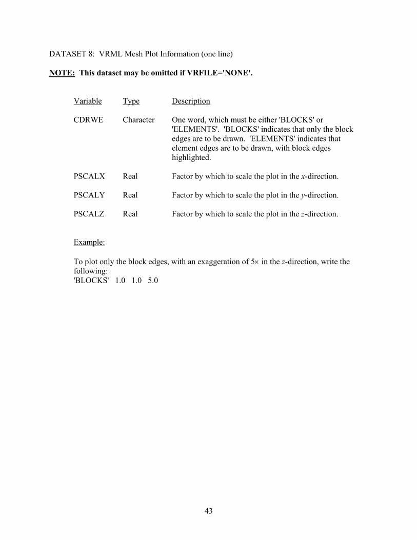
DATASET 8: VRML Mesh Plot Information (one line) NOTE: This dataset may be omitted if VRFILE='NONE'. Variable Type Description CDRWE Character One word, which must be either 'BLOCKS' or

'ELEMENTS'. 'BLOCKS' indicates that only the block edges are to be drawn. 'ELEMENTS' indicates that element edges are to be drawn, with block edges highlighted.

PSCALX Real Factor by which to scale the plot in the x-direction. PSCALY Real Factor by which to scale the plot in the y-direction. PSCALZ Real Factor by which to scale the plot in the z-direction.

Example: To plot only the block edges, with an exaggeration of 5× in the z-direction, write the following: 'BLOCKS' 1.0 1.0 5.0