sutured khovanov homology, hochschild - mathematics

SUTURED KHOVANOV HOMOLOGY, HOCHSCHILD HOMOLOGY,AND THE OZSVATH-SZABO SPECTRAL SEQUENCE

DENIS AUROUX, J. ELISENDA GRIGSBY, AND STEPHAN M. WEHRLI

Abstract. In [16], Khovanov-Seidel constructed a faithful action of the (m+ 1)–strand

braid group, Bm+1, on the derived category of left modules over a quiver algebra, Am.We interpret the Hochschild homology of the Khovanov-Seidel braid invariant as a direct

summand of the sutured Khovanov homology of the annular braid closure.

1. Introduction

In [14], Khovanov constructed an invariant of links in S3 that takes the form of a bigradedabelian group arising as the homology groups of a combinatorially-defined chain complex.The graded Euler characteristic of Khovanov’s link homology recovers the Jones polynomial.

In [1], Asaeda-Przytycki-Sikora showed how to extend Khovanov’s construction to obtainan invariant of links in any thickened surface with boundary, F . When F is an annulus, thetopological situation is particularly natural; the thickened annulus, A× I, can be identifiedwith the complement of a standardly-imbedded unknot in S3. As observed by L. Roberts[24], the data of the imbedding A × I ⊂ S3 endows the Khovanov complex associated toL ⊂ S3 with a filtration, and the resulting invariant of L ⊂ (A × I ⊂ S3) is the filteredchain homotopy type of the complex. The induced spectral sequence converges to Kh(L),the Khovanov homology of L ⊂ S3.

This filtered complex is particularly well-suited for studying braids up to conjugacy.Explicitly, letting Bm+1 denote the (m + 1)–strand braid group, we can form the annularclosure, σ ⊂ A × I, of any braid σ ∈ Bm+1, and the isotopy class of the resulting annularlink (hence, the filtered chain homotopy type of the Khovanov complex) is an invariant ofthe conjugacy class of σ ∈ Bm+1. Indeed, the homology of the associated graded complex,the so-called sutured annular Khovanov homology of L ⊂ A× I, detects the trivial braid forevery m ∈ Z≥0, though it cannot distinguish all pairs of non-conjugate braids (cf. [4]).

The main goal of this paper is to establish a relationship between the sutured Khovanovhomology of a braid closure and another “categorified” braid invariant appearing in workof Khovanov and Seidel. In [16], Khovanov-Seidel consider a family of graded associativealgebras, Am, each realized as the quotient of a path algebra by a collection of quadraticrelations. To each σ ∈ Bm+1 they associate a differential graded bimodule, Mσ, over Am,well-defined up to homotopy equivalence, and prove that tensoring withMσ over Am yieldsa well-defined endofunctor on Db(Am − mod), the bounded derived category of left Am–modules. By relating the action of Bm+1 on Db(Am − mod) to its action on the Fukayacategory of a certain symplectic manifold (the Milnor fiber of an Am–type singularity), theyprove that their categorical action is faithful, i.e.,Mσ

∼=M1 iff σ = 1. The Khovanov-Seidel

DA was partially supported by NSF grant DMS-1007177.

JEG was partially supported by NSF grant number DMS-0905848 and NSF CAREER award DMS-1151671.

SMW was partially supported by NSF grant number DMS-1111680.

1

2 DENIS AUROUX, J. ELISENDA GRIGSBY, AND STEPHAN M. WEHRLI

construction also gives rise to a braid conjugacy class invariant: the Hochschild homology ofAm with coefficients in Mσ, denoted HH(Am,Mσ).

Our main result is a proof that these two braid conjugacy invariants are closely-related;one is a direct summand of the other. To state our result more precisely, we first notethat while Khovanov homology is bigraded, sutured annular Khovanov homology is triply-graded (the extra filtration grading appropriately measures “wrapping” around the annulus).Denote by SKh(L; f) the sutured Khovanov homology in filtration grading f . We prove:

Theorem 5.1. Let σ ∈ Bm+1, and m(σ) ⊂ A× I the mirror of its annular closure.

SKh (m(σ);m− 1) ∼= HH (Am,Mσ) .

Informally, the Hochschild homology of the Khovanov-Seidel bimodule,Mσ, agrees withthe “next-to-top” graded piece of SKh(m(σ)).1 Moreover, up to an overall normalization,the bigrading on SKh(σ) agrees with a natural bigrading on HH (Am,Mσ) . This is madeexplicit in the more precise version of Theorem 5.1 stated in Section 5.

Those readers familiar with strongly-based mapping class bimodules in bordered Heegaard-Floer homology should recognize Theorem 5.1 as a Khovanov homology analogue of (the1–moving strand case of) [19, Thm. 7]. Indeed, letting Σ(σ) denote the double-cover ofS3 branched over σ, p : Σ(σ) → S3 the covering map, and KB the braid axis, one corol-lary of Theorem 5.1 is a new proof of the existence of a spectral sequence relating the“next-to-top” filtration grading of the sutured Khovanov homology of a braid closure tothe “next-to-bottom” Alexander grading of the knot Floer homology of the fibered link,p−1(KB). See Theorem 6.1 for a more precise statement and [24] (for even index, [8]) forthe original proof of this result.

We should also point out that the Khovanov-Seidel algebra is a special case (k = 1) of afamily of algebras Ak,n−k (where n = m+ 1), defined independently by Chen-Khovanov [6]and Stroppel [26] (see also [5]), that give rise to a categorification of the Uq(sl2) Reshetikhin-Turaev invariant of tangles (cf. [7, Thm. 66]). These algebras are subquotient algebras ofKhovanov’s arc algebra Hn [15] and can be identified with endomorphism algebras of pro-jective generators of certain blocks, Ok,n−k, of category O. They also admit a geometricinterpretation in terms of convolution algebras of 2–block Springer fibers [27]. As in theKhovanov-Seidel setting, one obtains, for each k, a categorified braid (indeed, tangle) invari-ant that takes the form of a (derived equivalence class of a) bimodule,Mk

σ, over the algebraAk,n−k. The following conjecture, generalizing Theorem 5.1, arose during conversationswith Catharina Stroppel:

Conjecture 1.1. Let σ ∈ Bn, and m(σ) ⊂ A× I the mirror of its annular closure.

SKh(m(σ);n− 2k) ∼= HH(Ak,n−k,Mkσ)

Establishing this conjecture may be useful for computational purposes, since modifyingexisting Khovanov homology programs to compute sutured Khovanov homology should bestraightforward.

Acknowledgments: We thank John Baldwin, Tony Licata, and Catharina Stroppel fora number of interesting conversations, as well as Robert Lipshitz for explaining how to obtainProposition 6.3, generalizing [19, Thm. 7], from work of Rumen Zarev [28]. We would alsolike to thank MSRI and the organizers of the semester-long program on Homology Theoriesof Knots and Links, during which a portion of this work was completed.

1It is an immediate consequence of the definitions (see Section 4.1) that if σ ∈ Bm+1, then SKh(bσ; f) = 0unless f ∈ {−(m+ 1),−(m− 1), . . . ,m− 1,m+ 1}.

SKH AND HH 3

mi−1 i0

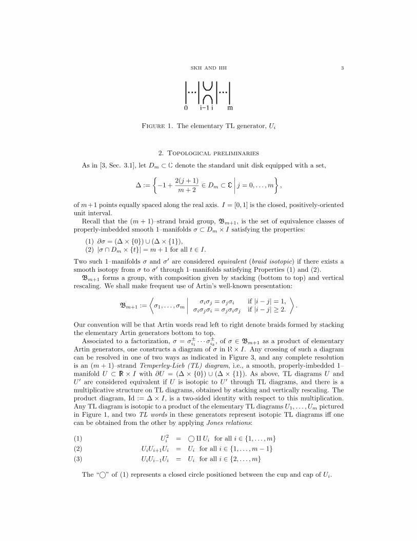
Figure 1. The elementary TL generator, Ui

2. Topological preliminaries

As in [3, Sec. 3.1], let Dm ⊂ C denote the standard unit disk equipped with a set,

∆ :={−1 +

2(j + 1)m+ 2

∈ Dm ⊂ C j = 0, . . . ,m},

of m+1 points equally spaced along the real axis. I = [0, 1] is the closed, positively-orientedunit interval.

Recall that the (m + 1)–strand braid group, Bm+1, is the set of equivalence classes ofproperly-imbedded smooth 1–manifolds σ ⊂ Dm × I satisfying the properties:

(1) ∂σ = (∆× {0}) ∪ (∆× {1}),(2) |σ ∩Dm × {t}| = m+ 1 for all t ∈ I.

Two such 1–manifolds σ and σ′ are considered equivalent (braid isotopic) if there exists asmooth isotopy from σ to σ′ through 1–manifolds satisfying Properties (1) and (2).

Bm+1 forms a group, with composition given by stacking (bottom to top) and verticalrescaling. We shall make frequent use of Artin’s well-known presentation:

Bm+1 :=⟨σ1, . . . , σm

σiσj = σjσi if |i− j| = 1,σiσjσi = σjσiσj if |i− j| ≥ 2.

⟩.

Our convention will be that Artin words read left to right denote braids formed by stackingthe elementary Artin generators bottom to top.

Associated to a factorization, σ = σ±i1 · · ·σ±ik

, of σ ∈ Bm+1 as a product of elementaryArtin generators, one constructs a diagram of σ in R × I. Any crossing of such a diagramcan be resolved in one of two ways as indicated in Figure 3, and any complete resolutionis an (m + 1)–strand Temperley-Lieb (TL) diagram, i.e., a smooth, properly-imbedded 1–manifold U ⊂ R × I with ∂U = (∆ × {0}) ∪ (∆ × {1}). As above, TL diagrams U andU ′ are considered equivalent if U is isotopic to U ′ through TL diagrams, and there is amultiplicative structure on TL diagrams, obtained by stacking and vertically rescaling. Theproduct diagram, Id := ∆ × I, is a two-sided identity with respect to this multiplication.Any TL diagram is isotopic to a product of the elementary TL diagrams U1, . . . , Um picturedin Figure 1, and two TL words in these generators represent isotopic TL diagrams iff onecan be obtained from the other by applying Jones relations:

U2i = ©q Ui for all i ∈ {1, . . . ,m}(1)

UiUi+1Ui = Ui for all i ∈ {1, . . . ,m− 1}(2)UiUi−1Ui = Ui for all i ∈ {2, . . . ,m}(3)

The “©” of (1) represents a closed circle positioned between the cup and cap of Ui.


3. Algebraic Preliminaries

We refer the reader to [12], [13], [25], [17], [18] for standard background on A∞ algebrasand modules. Terminology and notation are as in [3]. All algebras/modules we consider areover F := Z/2Z.

Notation 3.1. Given a bigraded vector space

V =⊕i,j∈Z

V(i,j),

(e.g., a differential graded module) and k1, k2 ∈ Z, V [k1]{k2} will denote the bigradedvector space whose first (homological) grading has been shifted down by k1 and whosesecond (internal) grading has been shifted up by k2.2 Explicitly,

(V [k1]{k2})(i−k1,j+k2) := V(i,j).

Notation 3.2. If V is a bigraded vector space, k ∈ Z≥0, and W := F(0,−1) ⊕ F(0,1), thenwe will use the notation ©kV to denote the bigraded vector space V ⊗W⊗k.

Notation 3.3. Let A and B be A∞ algebras. We will denote by D∞(A) (resp., by D∞(Aop),D∞(A−Bop)) the category whose objects are homologically unital A∞ left– (resp., right–,bi-) modules over A (resp., over A, over A–B) and whose morphisms are A∞ homotopyclasses of A∞ morphisms.

Definition 3.4. Let A,B, and C be A∞ algebras, M ∈ D∞(A− Bop), and N ∈ D∞(B −Cop). The derived A∞ tensor product, M⊗BN , is the well-defined object of D∞(A− Cop)represented by the A∞ bimodule over A–C with underlying vector space

∞⊕k=0

M ⊗B⊗k ⊗N,

whose differential (m(0|1|0) structure map) is given in terms of the structure maps mM , mB ,and mN by

mM e⊗BN(0|1|0) :=

∑i1≤k

mM(0|1|i1) ⊗ Id⊗k−i1+1 +

∑i2≤k

Id⊗k−i2+1 ⊗mN(i2|1|0)

+∑

1≤j1<j2≤k

Id⊗j1 ⊗mBj2−j1 ⊗ Id⊗k−j2+2

and whose higher (i1 > 0 or i2 > 0) A∞ structure maps,

mM e⊗BN(i1|1|i2) : A⊗i1 ⊗

(M ⊗B⊗k ⊗N

)⊗ C⊗i2 →

⊕0≤j≤k

M ⊗B⊗k−j ⊗N,

are given by

mM e⊗BN(i1|1|i2) :=

∑

0≤j≤kmM(i1|1|j) ⊗ Id⊗k−j+1 if i2 = 0,∑

0≤j≤k Id⊗k−j+1 ⊗mM(j|1|i2) if i1 = 0,

0 otherwise.

2The difference in shift conventions for homological versus internal gradings is unfortunate, but standardin the literature. In particular, they coincide with those in [16], to which we frequently refer.

SKH AND HH 5

Definition 3.5. Let A be an A∞ algebra and M ∈ D∞(A−Aop). The Hochschild homologyof A with coefficients in M , denoted HH(A,M), is the derived A∞ self-tensor product ofM . Explicitly, it is the homology of the chain complex with underlying vector space:

m⊕k=0

A⊗k ⊗M

and differential∂(a1 ⊗ . . .⊗ ak ⊗m) :=∑

0≤i1,i2i1+i2≤k

ai2+1 ⊗ . . .⊗ ak−i1 ⊗mM(i1|1|i2)(ak−i1+1 ⊗ . . .⊗ ak ⊗m⊗ a1 ⊗ . . .⊗ ai2)

+∑

1≤j1<j2≤k

a1 ⊗ . . .⊗mAj2−j1+1(aj1 ⊗ . . .⊗ aj2)⊗ aj2+1 ⊗ . . .⊗ ak ⊗m

When A is an ordinary associative algebra and M is a dg bimodule, the above definitionagrees with the “classical” definition of Hochschild homology:

Definition 3.6. Let A be an associative algebra and M a dg bimodule over A. Notingthat M (resp., A) can be viewed as a left (resp., right) module over Ae := A⊗Aop, the nth(classical) Hochschild homology of A with coefficients in M is

HHn(A,M) := TorAe

n (A,M).

In particular, to compute HH(A,M) one chooses a resolution

R(A)→ A

of A by projective right Ae modules, and

HHn(M) := Hn(R(A)⊗Ae M).

Standard arguments in homological algebra imply that the homology is independent of thechosen resolution. When R(A) is the bar resolution, we obtain:

HHn(A,M) := Hn( · · · ∂4 // A⊗3 ⊗M∂3 // A⊗2 ⊗M

∂2 // A⊗M∂1 // M ),

where∂i(a1 ⊗ . . .⊗ ai ⊗m) := (a1 ⊗ . . .⊗ ai ⊗ ∂Mm)+

(a1a2 ⊗ a3 ⊗ . . . ai ⊗m) + (a1 ⊗ a2a3 ⊗ . . . ai ⊗m) + . . .+ (a2 ⊗ a3 ⊗ . . .⊗ma1),and ∂M is the internal differential on M .

Since the higher structure maps of A and M are assumed to be zero, the complex de-scribed in Definition 3.5 agrees with this one. Accordingly, we shall use the definitionsinterchangeably when discussing the Hochschild homology of an ordinary associative alge-bra with coefficients in a dg bimodule.

Lemma 3.7. Let A and B be A∞ algebras. We have

HH(A,M⊗BN) ∼= HH(B,N⊗AM)

for any A∞ A–B bimodule M and A∞ B–A bimodule N .

Proof. The Hochschild complexes described in Definition 3.5 are chain isomorphic, via the(F–linear extension of) the canonical identification

(a1 ⊗ . . .⊗ ak)⊗m⊗ (b1 ⊗ . . .⊗ b`)⊗ n←→ (b1 ⊗ . . .⊗ b`)⊗ n⊗ (a1 ⊗ . . .⊗ ak)⊗m.�


Corollary 3.8. Let A and B be A∞ algebras. Suppose that there exists an A∞ A–Bbimodule APB and an A∞ B–A bimodule BPA satisfying the property that

APB ⊗B BPA ∼= A ∈ D∞(A−Aop).

Then for any M ∈ D∞(A−Aop), we have

HH(A,M) ∼= HH(B,BPA ⊗A M ⊗A APB).

Proof. By Lemma 3.7 and the equivalence APB ⊗B BPA ∼= A, we have

HH(B,BPA ⊗A M ⊗A APB) ∼= HH(A,M ⊗A APB ⊗B BPA)∼= HH(A,M),

as desired. �

We will also make use of the following non-derived version of a self-tensor product for dgbimodules over an associative algebra.

Definition 3.9. Let A be an associative algebra (i.e., a dg algebra supported in a singlehomological grading) and let

M =(· · · //Mn

∂n //Mn+1// · · ·

)be a dg A–bimodule.

Then the coinvariant quotient complex of M is the complex:

Q(M) :=(· · · // Q(Mn)

Q(∂n) // Q(Mn+1) // · · ·),

where

Q(Mn) :=Mn

〈am−ma | a ∈ A,m ∈Mn〉,

and Q(∂n) is the induced differential on the quotient (well-defined, since ∂n is A–linear).

We have the following analogue of Lemma 3.7:

Lemma 3.10. Let A,B be associative algebras, and let M (resp., N ) be dg bimodules overA−B (resp., over B −A). The canonical F–linear map

Ψ : Q(M⊗B N )→ Q(N ⊗AM)

sending [m⊗ n] ∈ Q(M⊗A N ) to [n⊗m] ∈ Q(N ⊗BM) is a chain isomorphism.

Proof. Ψ is well-defined, since for any a ∈ A, b ∈ B,m ∈M, n ∈ N we have

Ψ[mb⊗ n] = [n⊗mb] = [bn⊗m] = Ψ[m⊗ bn]

andΨ[am⊗ n] = [n⊗ am] = [na⊗m] = Ψ[m⊗ na].

Verifying that Ψ is a chain map (with canonical inverse) is similarly routine. �

4. Sutured annular Khovanov homology and Khovanov-Seidel bimodules

We begin by reviewing the definition of sutured annular Khovanov homology in [1] (seealso [24], [8]) as well as the construction of Khovanov-Seidel in [16].

SKH AND HH 7

X O

γ0

Figure 2. Pictured above are two diagrams of an annular link, L ⊂ A× I,one on A×

{12

}(left) and one on S2 equipped with two distinguished points,

O and X (right). The oriented arc, γ0, specifies the “f” (filtration) gradingon the Khovanov complex associated to the annular link.

"−1" resolution link diagram

crossing

"1" resolution

(1,−1) resolution

1

2

Figure 3. If the k crossings of a link diagram have been ordered, we canassociate to each vertex, (v1, . . . , vk) ∈ {−1, 1}k, of the k–cube a completeresolution of the diagram as indicated.

4.1. Sutured annular Khovanov homology. Sutured annular Khovanov homology isan invariant of links in a solid torus (equipped with a fixed identification as a thickenedannulus), defined as follows.

Let A denote an oriented annulus and I = [0, 1] the closed, positively oriented, unitinterval. Any link L ⊂ A × I admits a diagram on A × { 1

2}, which can equivalently beviewed as a diagram on S2 − {O,X}, where O,X are two distinguished points (the northand south poles, e.g.). See Figure 2.

By forgetting the data of the X basepoint, one obtains a diagram of L on D := S2−N(O).At this point, one can construct the (bigraded) Khovanov complex as normal by orderingthe k crossings of the diagram of L and assigning to the diagram its k–dimensional cubeof resolutions, [−1, 1]k, whose vertices, ~v = (v1, . . . , vk) ∈ {−1, 1}k, correspond to completeresolutions as in Figure 3.

If we now remember the data of the X basepoint, we may choose an oriented arc, γ0,from X to O missing all crossings of the diagram. As described in [9, Sec. 4.2], thegenerators of the Khovanov complex are in 1 : 1 correspondence with enhanced (i.e., oriented)resolutions, so from the data of the oriented arc we obtain an extra “f” (filtration) gradingon the complex from the algebraic intersection number of the oriented arc with the orientedresolution. Roberts proves ([24, Lem. 1]), that the Khovanov differential is non-increasing


Figure 4. A radial slice of the homeomorphism Dm × S1 ≈ A× I

in this extra grading, so one obtains a filtration of the Khovanov complex, CKh(L):

0 ⊆ . . . ⊆ Fn−1 ⊆ Fn ⊆ Fn+1 ⊆ . . . ⊆ CKh(L),

whose nth subcomplex is given by:

Fn := ⊕f≤nCKh(L; f).

The sutured annular Khovanov homology of L is then defined to be the homology of theassociated graded complex:

SKh(L) :=⊕n∈Z

SKh(L;n) :=⊕n∈Z

H∗

(FnFn−1

).

A concrete description of the sutured annular chain complex is given in [24, Sec. 2]. Seealso [8] and [9].

In the present work, we will be interested in the special case when L is the annular braidclosure, σ, of a braid, σ. Precisely, if σ ⊂ Dm × I is a braid, then we obtain σ ⊂ A× I, bygluing Dm×{0} to Dm×{1} by the identity diffeomorphism and choosing the identificationDm × S1 ≈ A× I that on each radial slice agrees with the homeomorphism of Figure 4.

Note that if we view S3 as R3 ∪∞, there is a standard imbedding of the annular closureof σ as a link in the complement of the braid axis,

KB := {(r, θ, z) | r = 0} ∪∞ ⊂ S3,

via the homeomorphism identifying A× I with S3 −N(KB):

A× I = {(r, θ, z) r ∈ [1, 2], θ ∈ [0, 2π), z ∈ [0, 1]} ⊂ S3.

In preparation for establishing a correspondence with the Khovanov-Seidel bimodulesdescribed in the next section, we now give an explicit description of the sutured annularchain complex of a factorized annular braid closure. Order the k crossings of σ = σ±i1 · · ·σ

±ik

from bottom to top, as read from left to right (where σ±i is as pictured in 6), and assignthe same ordering to the crossings of the annular diagram of σ ⊂ A× I. Endow σ with thebraid orientation.

Now consider the k–dimensional cube, [−1, 1]k, whose vertices are indexed by k–tuples~v = (v1, . . . , vk) ∈ {−1, 1}k. Letting εj(σ±i1 · · ·σ

±ik

) ∈ {−1, 1} denote the exponent on thejth term in the product, we can now identify the vertex ~v of the k–cube with the annularclosure of the TL diagram, Ni1 · · ·Nik , where:

(4) Nij :={Uij if vjεj = 1, andId if vjεj = −1,

Moreover, if there is a directed edge from a vertex ~v to a vertex ~w in the k–cube then~v, ~w agree except at a single entry at (say) the j–th position, where vj = −1 and wj = +1.

SKH AND HH 9

m0 1

...2

Figure 5. The oriented graph Γm used in the definition of the algebra Am

The map assigned to this edge is one of the split/merge maps described in [24, Sec. 2],depending on the topological configuration of the splitting/merging circles.

Let n+ (resp., n−) denote the number of positive (resp., negative) crossings of σ. The(h)omological, (q)uantum, and (f)iltration gradings of a sutured annular Khovanov gener-ator, x, is given in terms of its associated oriented resolution (enhanced Kauffman state),S(x), by:

h(x) = −n− +12

k∑i=1

(1 + vi(x))

q(x) = (n+ − 2n−) + CCW(S(x))− CW(S(x)) + h(x)f(x) = [γ0] · [S(x)],

where “·” denotes algebraic intersection number, and CCW(S(x)) (resp., CW(S(x))) denotesthe number of components of S(x) oriented counter-clockwise (resp., clockwise).

Note that if σ ∈ Bm+1, then SKh(σ; k) = 0 for k 6∈ {−(m+1),−(m−1), . . . ,m−1,m+1}(cf. [3, Prop. 7.1]), so we will sometimes refer to SKh(σ;m− 1) as the next-to-top filtrationlevel of SKh(σ).

4.2. Khovanov-Seidel bimodules. Let Γm be the oriented graph (quiver) with• vertices labeled 0, . . . ,m and• a pair of oppositely–oriented edges connecting each pair of adjacent vertices, as in

Figure 5.Recall that, given any oriented graph Γ, one defines its path algebra as the algebra whose

underlying vector space is freely generated by the set of all finite-length paths in Γ, andmultiplication is given by concatenation (the product of two non-composable paths is 0).

The algebra Am is then defined as a quotient of the path algebra of Γm by the collectionof relations

(i− 1|i|i+ 1) = (i+ 1|i|i− 1) = 0, (i|i+ 1|i) = (i|i− 1|i), (0|1|0) = 0

for each 1 ≤ i ≤ m − 1. In the above, following [16], we have labeled each path in Γm bythe complete ordered tuple of vertices it traverses. So, for instance, (i|i + 1|i) denotes thepath that starts at vertex i, moves right to i+ 1, then returns to i.

The path algebra of Γm is further endowed with an internal grading by negative pathlength. As the above relations are homogenous with respect to this grading, it descends tothe quotient, Am.3

The collection, {(i)|i ∈ 0, . . . ,m}, of constant paths are mutually orthogonal idempotentswhose sum, 1 =

∑mi=0(i), is the identity in Am. There are corresponding decompositions

3The reader should be warned that we are using a different internal grading than the one considered in

[16] and [3]. It is this negative path length grading and not Khovanov-Seidel’s steps-to-the-left grading thatis most directly related to Khovanov homology. Note also that Am is Koszul with respect to the positive

path length grading, cf. [26].


...... ......m0 i−1 m0 ii−1i

σ−iσ+i

Figure 6. The elementary Artin braid group generators

of Am as a direct sum of projective left-modules Am =⊕m

i=0Am(i) (resp., projective right-modules Am =

⊕mi=0(i)Am). As in [16], we denote Am(i) (resp., (i)Am) by Pi (resp., iP ).

Note that Pi (resp., iP ) is the set of all paths ending at i (resp., beginning at i).Khovanov-Seidel go on to construct a braid group action on Db(Am), the bounded derived

category of left Am–modules, by associating to each elementary braid word σ±1i (pictured

in Figure 6) a differential bimoduleMσ±iand to each braid, σ := σi1

± · · ·σik±, decomposedas a product of elementary braid words, the differential bimodule

Mσ =Mσ±i1⊗Am . . .⊗AmMσ±ik

.

Specifically, they associate to σ+i the differential bimodule

Mσ+i

:= Pi ⊗ iP{1}βi // Am{1} ,

where βi is the Am–bimodule map induced by the assignment βi((i)⊗ (i)) = (i), and to σ−ithe differential bimodule

Mσ−i:= Am

γi // Pi ⊗ iP{2} ,where

γi(1) = (i− 1|i)⊗ (i|i− 1) + (i+ 1|i)⊗ (i|i+ 1) + (i)⊗ (i|i− 1|i) + (i|i− 1|i)⊗ (i).

Suppose now that we begin with σ ∈ Bm+1, along with a decomposition σ = σ±i1 · · ·σ±ik

.Noting that the Khovanov-Seidel braid module Mσ is a tensor product (over Am) of two-term complexes, each of which is a mapping cone of an Am–module map between thebimodule (Pi ⊗ iP ) assigned to the i–th elementary Temperley-Lieb (TL) object and thebimodule (Am) assigned to the trivial TL object, we have a “cube of resolutions” descriptionof Mσ in terms of the given decomposition of σ as follows which is similar in structure tothe cube of resolutions description of the sutured annular Khovanov homology of σ ⊂ A×I.

Order the k crossings of the braid diagram σ = σ±i1 · · ·σ±ik

in the direction of the braidorientation (by convention, from bottom to top as read from left to right). Now considerthe k–dimensional cube, [−1, 1]k, whose vertices are indexed by k–tuples ~v = (v1, . . . , vk) ∈{−1, 1}k. Letting εj(σ±i1 · · ·σ

±ik

) ∈ {−1, 1} denote the exponent on the jth term in theproduct, we can now (modulo bigrading shifts, specified in Lemma 4.1) identify the vertex~v of the k–cube with the term, Ni1 ⊗Am . . .⊗Am Nik , of the complex Mσ, where:

(5) Nij :={

Am if vjεj = 1, andPij ⊗ ijP if vjεj = −1,

Moreover, if there is a directed edge from a vertex ~v to a vertex ~w in the k–cube then~v, ~w agree except at a single entry at (say) the j–th position. The map assigned to this edgeis then

Id⊗ . . .⊗{βijγij

}⊗ . . .⊗ Id

SKH AND HH 11

according to whether εj ={

+1−1

}.

As the homological and quantum grading shifts of generators at vertices in this “cube ofresolutions” complex for Mσ = Mσ±i1

···σ±ikare somewhat cumbersome, we take a moment

to record them here.

Lemma 4.1. The bigraded Khovanov-Seidel bimodule associated to the vertex ~v ∈ {−1, 1}kin the above cube of resolutions is

(Ni1 ⊗Am . . .⊗Am Nik) [−~vh]{~vq},where

~vh :=k∑j=1

12

(vj + 1),

and

~vq = ~vh +k∑j=1

12

(1− vjεj).

Proof. By definition, ~vh is the number of 1’s in the k–tuple ~v ∈ {−1, 1}k, so the firststatement follows.

To compute ~vq, note that we get an overall +1 shift for every j ∈ {1, . . . , n} satisfyingεj = 1 and an extra +2 shift for each j ∈ {1, . . . , k} satisfying εj = −1 and vj = 1. It followsthat

~vq =k∑j=1

12

(εj + 1) +k∑j=1

−12

(εj − 1)(vj + 1)

= ~vh +k∑j=1

12

(1− vjεj),

as desired. �

Note that∑kj=1

12 (1 − vjεj) is the length of the TL word in elementary TL generators

corresponding to the vertex ~v. Equivalently, it is the number of terms of the form (Pij⊗ ijP )in the corresponding tensor product Ni1 ⊗Am . . .⊗Am Nik .

5. Main Theorem

In the following,• Mσ denotes the Khovanov-Seidel bimodule associated to a braid, σ = σ±i1 · · ·σ

±ik∈

Bm+1 as described in Section 4.2,• SKh(m(σ);m − 1) denotes the “next-to-top” (f)iltration grading of the sutured

Khovanov homology of m(σ) ⊂ A × I, the mirror (all crossings reversed) of thebraid closure, σ, in A× I, as in Section 4.1.

Theorem 5.1. Let σ ∈ Bm+1 and m(σ) ⊂ A× I the mirror of its annular closure.

SKh (m(σ);m− 1) ∼= HH (Am,Mσ) [n−]{(m− 1) + n+ − 2n−}as bigraded vector spaces.

Remark 5.2. The mirror of σ appears on the left-hand side of the equivalence abovebecause of differing braid conventions in [14] and [16], cf. (4) and (5).


i-1

Am Pi ⊗ iP

i

Figure 7. The (derived equivalence class of the) dg Am–bimodule associ-ated to an elementary Artin braid σ±i is a (grading-shifted) mapping coneof the bimodules Am and Pi ⊗ iP ; the former is identified with the trivialTL object (left) and the latter is identified with the ith elementary TLobject (right).

Proof. We prove, in Proposition 5.3, that

SKh (m(σ);m− 1) ∼= H∗(Q(Mσ))[n−]{(m− 1) + n+ − 2n−},

where H∗(Q(Mσ)) is the homology of the coinvariant quotient module4 (Definition 3.9) of

Mσ :=Mσ±i1···σ±ik

.

But Proposition 5.4 tells us that

H∗(Q(Mσ)) ∼= HH∗(Am,Mσ),

as desired. �

Proposition 5.3. Let σ ∈ Bm+1 be a braid of index m+1 and σ ⊂ A× I its closure. Then

SKh (m(σ);m− 1) ∼= H∗ (Q (Mσ)) [n−]{(m− 1) + n+ − 2n−}

as bigraded vector spaces.

Proof. As noted in Section 4.2, the Khovanov-Seidel complex Mσ (and, hence, its coin-variant quotient complex Q(Mσ)) has a description in terms of a “cube of resolutions,” byidentifying Am with the trivial TL object and Pi⊗ iP with the i–th elementary TL object aspictured in Figure 7. The complex CKh(m(σ) ⊂ A×I) whose homology is SKh(σ) (denotedC(m(σ) ⊂ A× I) in [24, Sec. 2]–see also [1], [8, Sec. 4]) is also described in terms of a cubeof resolutions. Therefore, to prove that SKh(m(σ);m−1) coincides with Q (Mσ) (up to thestated grading shift) it suffices to verify that the two cubes of resolutions assign isomorphicbigraded F–vector spaces to the vertices and that, with respect to this isomorphism, theedge maps agree.

We begin with the vertices of the cube, comparing case-by-case:• the coinvariant quotient, Q (Ni1 ⊗Am . . .⊗Am Nik), of the Khovanov-Seidel bimod-

ule associated to a vertex, and• the F–vector space associated to the corresponding vertex in the “next-to-top” grad-

ing of the sutured Khovanov complex, CKh(m(σ);m− 1).See Figure 8 for TL diagrams associated to the various cases.

4It is proven in [16] that the homotopy equivalence class of Mσ does not depend on the chosen factor-ization of σ as a product of elementary braids. Since any homotopy equivalence descends to the coinvariant

quotient, we are justified in suppressing the factorization from the notation.

SKH AND HH 13

Case V1 Case V3 Case V4Case V2

Figure 8. We have enumerated above the different types of TL diagramsthat can appear at the vertices of a cube of resolutions.

In what follows, we shall always assume that we have used the isomorphism

M ⊗Am Am ∼= Am ⊗Am M ∼= M

to eliminate extraneous copies of Am in the tensor product associated to a vertex. Wheneverwe refer to a trivial (resp., nontrivial) circle in a resolution of the annular closure, wemean a component of the resolution that represents the trivial (resp., nontrivial) element ofH1(A;Z/2Z).

Case V1: Ni1 ⊗Am . . .⊗Am Nik ∼= Am

Khovanov-Seidel coinvariant quotient:Note that

Am =m⊕

i,j=0

iPj

where iPj := iP ⊗Am Pj . The coinvariant quotient, Q(Am) is, by definition, the quotient ofthe (dg) bimodule Am by the ideal generated by the image of the map φ : Am ⊗Am → Amdefined by φ(a⊗ b) = ab+ ba.

Therefore any element of iPj for i 6= j becomes 0 when we pass to Q(Am), since eachsuch element can be expressed as φ[(i)⊗ (i| . . . |j)]. Furthermore, any element of iPi of theform (i|i− 1|i) = (i|i+ 1|i) is also 0 in Q(Am), since we have

(i|i− 1|i) = (i− 1|i|i− 1) + φ[(i|i− 1)⊗ (i− 1|i)].Now, noting that (i − 1|i|i − 1) = (i − 1|i − 2|i − 1) ∈ Am and iterating, we see that

(i|i− 1|i) + (0|1|0) is in the image of φ, but (0|1|0) = 0 ∈ Am.The only possible nonzero elements of Q(Am) are therefore the idempotents, {(i) ∈ iPi}.

But these can only be decomposed as (i) ⊗ (i) ∈ Am ⊗ Am, so we obtain no new relationsamong them when we pass to the coinvariant quotient.

We conclude that the vector space associated to a vertex of this type is (m + 1)–dimensional, with basis given by the idempotents (0), (1), . . . , (m). In other words, theKhovanov-Seidel coinvariant quotient complex assigns the (grading-shifted) bigraded vectorspace

Fm+1(~vh,~vq)

[n−]{(m− 1) + (n+ − 2n−)}

to the vertex ~v = (v1, . . . , vk) ∈ {−1, 1}k .

Sutured annular Khovanov complex:The vertex associated to the closure of the trivial TL object in the cube of resolutions

for CKh(m(σ);m − 1) is also (m + 1)–dimensional, since the resolution consists of m + 1nontrivial circles. The vector space associated to this vertex in the f grading m − 1 (the


“next-to-top” one) has a basis given by the m + 1 enhanced resolutions where exactly oneof the circles has been labeled v−, and the rest have been labeled v+. The bigraded vectorspace associated to the sutured Khovanov complex at vertex ~v is therefore:

Fm+1(~vh,(m−1)+~vh)[n−]{(n+ − 2n−)}.

But ~vh = ~vq in this case (cf. Lemma 4.1), so the two bigraded vector spaces agree.

Isomorphism:For i = 0, 1, . . . ,m, let θi denote the basis element of CKh(m(σ);m− 1) described above

whose ith circle is labeled v−. Then the linear map Φ : Q(Am)→ CKh(m(σ);m− 1):

Φ[(i)] ={θi if i = 0, andθi + θi−1 otherwise

is an isomorphism of bigraded F–vector spaces (strategically chosen so that the boundarymaps along the edges of the cube will agree).

Case V2: Ni1 ⊗Am . . .⊗Am Nik = (Pij1 ⊗ ij1P )⊗Am . . .⊗Am (Pijn ⊗ ijn

P ), where ij1 = ijn(We allow here the possibility that n = 1.)

Khovanov-Seidel:Rewrite the above tensor product as:

Pij1 ⊗ (ij1P ⊗Am Pij2 )⊗ . . .⊗ (ijn−1P ⊗Am Pijn )⊗ ijn

P

as in the proof of [16, Thm. 2.2], and note that

aP ⊗Am Pb =

SpanF{(a), (a|a− 1|a)} if |a− b| = 0,

SpanF{(a|b)} if |a− b| = 1, and0 if |a− b| > 1.

The corresponding Khovanov-Seidel bimodule is therefore 0 if there exists a ∈ {1, . . . , n−1} such that |ija − ija+1 | > 1. Now suppose there exists no such adjacent pair. Then if theassociated TL diagram has ` closed components, we claim that its closure will have:

• `+ 1 trivial closed circles and• m− 1 additional nontrivial circles.

That there are ` + 1 trivial closed circles in the closure is clear. To see that there areexactly m− 1 nontrivial circles in the closure, proceed by induction on n, the length of theassociated TL word. The base case (n = 1) is quickly verified. If n > 1, the assumptions

(1) There exists no a ∈ {1, . . . , n− 1} such that |ija − ija+1 | > 1, and(2) ij1 = ijn

imply that there exists some subword of the TL word that can be replaced by a shortersubword using one of the Jones relations: (1)-(3), and the claim follows.

Corresponding applications of [16, Thm 2.2]5 now allow us to replace the original Khovanov-Seidel bimodule with the quasi-isomorphic bimodule ©` (Pij1 ⊗ ij1

P ){−(n− 1)}.We therefore need only understand Q(Pij1 ⊗ ij1

P ). An analysis similar to the one con-ducted in Case V1 implies that Q(Pij1 ⊗ ij1P ) is free of rank 2, generated by (ij1)⊗(ij1) and(ij1)⊗ (ij1 |ij1 − 1|ij1) (identified with (ij1 − 1|ij1)⊗ (ij1 |ij1 − 1) and (ij1 |ij1 − 1|ij1)⊗ (ij1)in the coinvariant quotient module).

5Note that, since we are using the negative path length rather than steps-to-the-left grading, we have{−2} rather than {1} shifts on the RHS of [16, Eqns. 2.2-2.4].

SKH AND HH 15

We conclude that the (grading-shifted) Khovanov-Seidel coinvariant quotient associatedto a vertex of this type is 0 if there exists a ∈ {1, . . . , n− 1} such that |ija − ija+1 | > 1, and

©`+1F(~vh,~vq−n)[n−]{(m− 1) + (n+ − 2n−)}otherwise.

Sutured Khovanov:Suppose that there exists a ∈ {1, . . . , n− 1} such that |ija − ija+1 | > 1. Then the closure

of the corresponding TL diagram can have no more than m − 3 nontrivial circles. Thevector space associated to a vertex of this type in this case is therefore 0, as it is in theKhovanov-Seidel setting.

Now suppose there exists no such adjacent pair. As explained above, if the associatedTL diagram has ` closed components, its closure will have ` + 1 trivial closed circles andm− 1 additional nontrivial circles.

The CKh(m(σ);m − 1) vector space therefore has a basis in 1 : 1 correspondence withenhanced resolutions whose (m−1) nontrivial circles have all been labeled v+ and the (`+1)trivial circles have been labeled with either w±. The associated (grading-shifted) bigradedvector space is therefore:

©`+1F(~vh,(m−1)+~vh)[n−]{n+ − 2n−}.

Since n =∑kj=1(1− vjεj) (cf. Lemma 4.1), the two bigraded vector spaces agree.

Isomorphism:If there exists a ∈ {1, . . . , n−1} with |ija−ija+1 | > 1, the vector spaces (and isomorphism)

are trivial.Otherwise, each of the (`+ 1) trivial circles in the closure of the TL diagram corresponds

to either an adjacent pair· · · ⊗ (ijaP ⊗Am Pija+1

)⊗ · · ·with ija = ija+1 or to the pair of outer terms

Pij1 ⊗ . . .⊗ ijnP,

which by assumption also satisfy ij1 = ijn .In fact, the basis elements of Q(Mσ) are in 1 : 1 correspondence with labelings of

the corresponding resolved diagram, where each trivial circle is labeled with either thelength 0 path (ija) or the length 2 path (ija |ija − 1|ija). Similarly, the basis elements ofCKh(m(σ);m−1) are in 1 : 1 correspondence with labelings of the resolved diagram, whereeach trivial circle is labeled with either a w+ or a w−.

We therefore obtain an isomorphism

Φ : Q((Pij1 ⊗ ij1P )⊗Am . . .⊗Am (Pijn ⊗ ijn

P ))→ CKh(σ;m− 1)

by identifying the length 0 (resp., length 2) path labels on the Khovanov-Seidel side withthe w+ (resp., w−) labels on the sutured Khovanov side.

Case V3: Ni1⊗Am . . .⊗AmNik = (Pij1⊗ij1P )⊗Am . . .⊗Am(Pijn⊗ijnP ), where |ij1−ijn | = 1.

Khovanov-Seidel:As in Case V2, the vertex is assigned 0 if there exists a ∈ {1, . . . , n − 1} such that

|ija − ija+1 | > 1. If there does not exist such an adjacent pair, then the analysis proceedsmuch as in Case V2. If the TL diagram has ` closed components, then its closure will have:

• ` trivial circles and• (m− 1) nontrivial circles,


by an inductive argument analogous to the one used in Case V2. The correspondingKhovanov-Seidel bimodule is isomorphic to 〈`〉(Pij1 ⊗ ijn

P ){−(n− 1)}.Since |ij1 − ijn | = 1, Q(Pij1 ⊗ ijn

P ) is 1–dimensional, generated by (ij1)⊗ (ijn |ij1).We conclude that the (grading-shifted) Khovanov-Seidel coinvariant quotient associated

to a vertex ~v of this type is 0 if there exists a ∈ {1, . . . , n − 1} such that |ija − ija+1 | > 1,and

〈`〉F(~vh,~vq−n)[n−]{(m− 1) + (n+ − 2n−)}otherwise.

Sutured Khovanov:As before, the vector space is 0 if there exists a ∈ {1, . . . , n−1} such that |ija−ija+1 | > 1.Otherwise, suppose that the associated TL diagram contains ` closed circles. Then, as

above, its closure will have ` trivial circles and (m − 1) nontrivial circles. One of these(m − 1) nontrivial circles is distinguished by the property that it contains both the cap ofthe first elementary TL element and the cup of the last elementary TL element in the tensorproduct.

Just as in Case V2, we therefore assign the bigraded vector space:

〈`〉F(~vh,(m−1)+~vh)[n−]{n+ − 2n−}

and define a completely analogous isomorphism Φ.

Case V4: Ni1⊗Am . . .⊗AmNik = (Pij1⊗ij1P )⊗Am . . .⊗Am (Pijn⊗ijnP ), where |ij1−ijn | > 1Here we see immediately that the coinvariant quotient of the Khovanov-Seidel bimodule

vanishes because there are no nonzero paths in Am between vertices separated by distancemore than 1, and the sutured annular Khovanov complex in f grading m− 1 vanishes sincethe closure of the corresponding TL object can have no more than (m−3) nontrivial circles.

We now verify that the edge maps agree. Again, this is a check of a finite numberof cases, each related to one of those pictured in Figure 9 by a finite sequence of cyclicpermutations and horizontal reflections. By applying Lemma 3.10, we may assume withoutloss of generality that the merge or split defining the edge map occurs in the final (top)term.

On the sutured Khovanov side, each of the edge maps corresponds to a map induced bya merge/split cobordism of one of the following types:

• Type I: Two nontrivial circles←→One trivial circle. This corresponds to merge/splitmaps of the form V ⊗ V ←→ W in the language of [24, Sec. 2]. Example E0 is ofthis type.• Type II: Two trivial circles ←→ One trivial circle. This corresponds to merge/split

maps of the form W ⊗W ←→W . Examples E1a and E2a are of this type.• Type III: One trivial and one nontrivial circle ←→ One nontrivial circle. This

corresponds to merge/split maps of the form V ⊗W ←→ V . Examples E1b, E2b,and E2c are of this type.

While describing Cases V2-V4, we noted that every trivial circle in the annular closureof a TL element arises as a result of a (cyclically) adjacent pair

· · · ⊗ iPi ⊗ · · · := · · · ⊗ (iP ⊗Am Pi)⊗ · · ·

in the associated Khovanov-Seidel tensor product. Moreover, “labelings” of the trivial circles(by either the length 0 or length 2 path) on the Khovanov-Seidel side correspond, via theisomorphism Φ, to labelings of the trivial circles (by either w+ or w−). It can now be seen

SKH AND HH 17

Case E0Case E1bCase E1a

Case E2a Case E2b Case E2c

Figure 9. We have enumerated (modulo vertical cyclic permutation andhorizontal reflection) all possible merges/splits occurring in nontrivial edgemaps in the cube-of-resolution models for the Khovanov-Seidel and suturedKhovanov complexes. The relevant merge/split is pictured in red, andthe cases are enumerated according to which TL object(s) are (cyclically)adjacent to the merge/split. Note that the edge map is necessarily 0 if thelocal configuration does not fall into one of the cases above, since one orboth of the vertices it connects must be 0 by the argument given in CasesV2–V4.

directly that the Khovanov-Seidel maps βi and γi behave exactly like the sutured Khovanovmerge/split maps in all cases. We include an explicit verification of this in Cases E0, E1a,and E1b. The other cases are similar.

Case E0: Pi ⊗ iP ←→ Am

“→”:On the Khovanov-Seidel side, recall from Case V2 that Q(Pi ⊗ iP ) has basis given by

{(i)⊗ (i), (i)⊗ (i|i− 1|i)}

and from Case V1 that Q(Am) has basis given by the idempotents

{(0), . . . , (m)}.

Moreover,

Q(βi)[(i)⊗ (i)] = (i)Q(βi)[(i)⊗ (i|i− 1|i)] = 0

On the sutured Khovanov side, the split map sends the generator whose trivial circle islabeled w+ (see Case V2) to θi + θi−1 (see Case V1). Under the isomorphism Φ describedin Cases V1 and V2, these maps agree.

“←”:


The only basis elements on the Khovanov-Seidel side with nontrivial image under Q(γi)are the idempotents (i− 1) and (i+ 1), both sent to

(i− 1|i)⊗ (i|i− 1) = (i+ 1|i)⊗ (i|i+ 1) = (i)⊗ (i|i− 1|i) ∈ Q(Pi ⊗ iP ).

On the sutured Khovanov side, the merge map sends the generators θi−1 and θi to thegenerator whose single trivial circle has been labeled w− and whose nontrivial circles haveall been labeled v+. Again, these maps agree under the isomorphism Φ.

Case E1a: ((Pi ⊗ iP )⊗Am (Pi ⊗ iP ))←→ (Pi ⊗ iP )

“→”:On the Khovanov-Seidel side, let iPi denote Pi ⊗Am iP and recall from Case V2 that

Q(Pi⊗ iPi⊗ iP ) has basis given by {(i)⊗a⊗ b | a, b ∈ {(i), (i|i− 1|i)}}, and the map Q(βi)is given by multiplication of the last two factors:

Q(βi)[(i)⊗ (i)⊗ (i)] = (i)⊗ (i)Q(βi)[(i)⊗ (i|i− 1|i)⊗ (i)] = Q(βi)[(i)⊗ (i)⊗ (i|i− 1|i)] = (i)⊗ (i|i− 1|i)

Q(βi)[(i)⊗ (i|i− 1|i)⊗ (i|i− 1|i)] = 0.

On the sutured Khovanov side, the map is given by multiplying the labels w± on thetwo trivial circles, which merge to form one. Now note that the isomorphism Φ identifiesa generator on the Khovanov-Seidel side whose second or third tensor factor is labeled (i)(resp., (i|i−1|i)) with a generator on the sutured Khovanov side whose first or second trivialcircle is labeled w+ (resp., w−). Moreover, the multiplication (merge) map in both settingsis the multiplication in F[x]/x2 via the identification of (i)↔ w+ with 1 and (i|i−1|i)↔ w−with x in F[x]/x2. The Khovanov-Seidel and sutured Khovanov maps therefore agree.

“←”: On the Khovanov-Seidel side, the map Q(γi) is given by:

Q(γi)[(i)⊗ (i)] = (i)⊗ (i)⊗ (i|i− 1|i) + (i)⊗ (i|i− 1|i)⊗ (i)Q(γi)[(i)⊗ (i|i− 1|i)] = (i)⊗ (i|i− 1|i)⊗ (i|i− 1|i)

which agrees with the split map on the sutured Khovanov side under the correspondence Φ,as described above.

Case E1b: ((Pi−1 ⊗ i−1P )⊗Am (Pi ⊗ iP ))←→ (Pi−1 ⊗ i−1P )

“→”: On the Khovanov-Seidel side, again let i−1Pi denote i−1P ⊗Am Pi and recall fromCase V3 that Q(Pi−1 ⊗ i−1Pi ⊗ iP ) is generated by (i− 1)⊗ (i− 1|i)⊗ (i|i− 1), and

Q(βi)[(i− 1)⊗ (i− 1|i)⊗ (i|i− 1)] = (i− 1)⊗ (i− 1|i− 2|i− 1).

On the sutured Khovanov side, we have a single nontrivial circle splitting into one trivialand one nontrivial circle, and the split map sends the generator v+ to the generator v+⊗w−.Under the isomorphism Φ from Cases V1 and V2, the two maps therefore agree.

“←”: On the Khovanov-Seidel side, we have

Q(γi)[(i− 1)⊗ (i− 1)] = (i− 1)⊗ (i− 1|i)⊗ (i|i− 1)Q(γi)[(i− 1)⊗ (i− 1|i− 2|i− 1)] = 0.

This agrees, under the isomorphism Φ, with the sutured Khovanov merge map, which sendsthe generator w+ ⊗ v+ to the generator v+ and the generator w− ⊗ v+ to 0.

�

SKH AND HH 19

Proposition 5.4. Let σ = σ±i1 · · ·σ±ik

be a braid. Then

HH∗(Am,Mσ) ∼= H∗(Q(Mσ)).

Proof. Given any resolution

R(Am) ∂ // Am := (· · ·R2∂2 // R1

∂1 // R0) ∂ // Am

of Am by projective right Aem := Am ⊗ Aopm modules, HH(Am,Mσ) is, by Definition 3.6,the homology of the complex R(Am)⊗AemMσ.

Note furthermore that R(Am) ⊗Aem Mσ has the structure of a double complex, whose“horizontal” differentials are of the form ∂∗⊗Aem 1, where ∂∗ is the differential in R(Am) andwhose “vertical” differentials are of the form 1⊗Aem d∗, where d∗ is the internal differentialin the complex Mσ. For example, the double complex for Mσ+

ilooks like:

· · ·R2 ⊗Aem (Pi ⊗ iP ){1} ∂2⊗1 //

1⊗βi��

R1 ⊗Aem (Pi ⊗ iP ){1} ∂1⊗1 //

1⊗βi��

R0 ⊗Aem (Pi ⊗ iP ){1}

1⊗βi��

· · ·R2 ⊗Aem Am{1}∂2⊗1 // R1 ⊗Aem Am{1}

∂1⊗1 // R0 ⊗Aem Am{1}

Let dh := ∂∗ ⊗Aem 1 (resp., dv := 1 ⊗Aem d∗) denote the horizontal (resp., vertical)differential on the complex Cσ := R(Am) ⊗Aem Mσ. There is a corresponding spectralsequence converging to

HH(Am,Mσ) := H∗(Cσ, dh + dv)

whose E2 term isH∗(H∗(Cσ, dh), dv).

Moreover, by choosing the bar resolution:

R(Am)→ Am := (· · ·A⊗4m

// A⊗3m

// A⊗2m ) // Am

we see thatQ(Mσ) is precisely the chain complex whose underlying vector space isH0(Cσ, dh)and whose differential is the induced differential, dv, on the quotient. Hence:

H∗(H0(Cσ, dh), dv) ∼= H∗(Q(Mσ))

Now we claim that Hn(Cσ, dh) = 0 for all n 6= 0. Since the induced differential on the E2

page must have a nonzero horizontal degree shift, the claim implies the desired result:

HH(Am,Mσ) ∼= H∗(Q(Mσ)),

since the spectral sequence must therefore collapse at the E2 stage.To prove the claim, observe first that the chain complex (Cσ, dh) splits as a direct sum of

chain complexes, one for each vertex of the cube of resolutions for Mσ. Accordingly, eachsubcomplex is of the form:

R(Am)⊗Aem (Ni1 ⊗Am . . .⊗Am Nik),

where

Nij :={

AmPij ⊗ ijP

depending on the vertex of the cube; hence, the homology of each such subcomplex is

HH(Am,Ni1 ⊗Am . . .⊗Am Nik).


m...

m...

1 0 10 **pm

q0

q1

qm

p0 p1

Figure 10. The matching and vanishing paths pi and qi in the base of theLefschetz fibration π : S → C.

Now note that Pk ⊗ `P is a projective Aem module for any k, ` ∈ {0, . . . ,m}, since

Am ⊗Am =m⊕

k,`=0

Pk ⊗ `P.

Since the tensor product functor is exact on projective modules, the Hochschild homologyof a projective bimodule is concentrated in degree 0. We conclude that whenever at leastone of the tensor factors Nij is of the form Pij ⊗ ijP , we have

Hn(R(Am)⊗Aem (Ni1 ⊗Am . . .⊗Am Nik)) = 0

for n 6= 0, as desired.The only remaining computation is HH(Am,Ni1 ⊗Am . . . ⊗Am Nik) in the case Ni1 =

. . . = Nik = Am, i.e., HH(Am, Am).Rather than computing HH(Am, Am) directly, we will exploit a relationship between

Am and another dg algebra, which we will call Bm, whose Hochschild homology is easy tocompute for algebraic reasons (its homology is directed). The motivation here comes fromthe geometric interpretation of the algebras Am and Bm in terms of the Fukaya category ofa certain Lefschetz fibration, described in [2], [25, Chp. 20], and recalled briefly in [3, Sec.3.5].

The definition of the dg algebra Bm can (and will) be given combinatorially, but sym-plectic geometers would do well to keep the following description in mind. Let

S = {(x, y, z) ∈ C3 |x2 + y2 = p(z)},

where p is a polynomial of degree m+1 whose roots are exactly the points 0, . . . ,m picturedin Figure 10. Then projection to the z coordinate gives a Lefschetz fibration π : S → C,for which the arcs p1, . . . , pm pictured in Figure 10 are matching paths and lift to La-grangian spheres PS1 , . . . , P

Sm ⊂ S. Meanwhile, the vanishing paths p0, q0, q1, . . . , qm deter-

mine Lefschetz thimbles PS0 , QS0 , . . . , Q

Sm. These are respectively spherical and exceptional

objects of the Fukaya category F(π) [25], in which End(PS0 ⊕ · · · ⊕ PSm) ' Am, whereasEnd(QS0 ⊕ · · · ⊕QSm) ' BKhm . The construction carried out here is equivalent to expressingthe elements of the exceptional collection QS0 , . . . , Q

Sm as twisted complexes built out of the

generators PS0 , . . . , PSm. See also [3, Sec. 3]. Note that in [3], the subscript m was dropped

from the notation for Bm, BKhm , and BHFm .The dg algebra Bm can be described combinatorially by:

Bm :=m⊕

i,j=0

HomAm(Qi, Qj) =m⊕

i,j=0

iQj ,

SKH AND HH 21

where

Qi := P0

·(0|1) // P1

·(1|2) // . . . ·(i−1|i)// Pi ,

and

iQj :=

0P0

·(0|1) //0P1

·(1|2) // . . .·(j−1|j)// 0Pj

1P0//

(0|1)·

OO

1P1//

OO

. . . //

OO

1Pj

OO

· · ·

(1|2)·

OO

// · · ·

OO

// · · ·

OO

// · · ·

OO

iP0//

(i−1|i)·

OO

iP1//

OO

. . . //

OO

iPj

OO

.

In the above, iPj := HomAm(Pi, Pj) denotes the subspace of Am generated by pathsbeginning at i and ending at j, and the horizontal (resp., vertical) maps are given by right(resp., left) multiplication by the appropriate length-one path, as indicated in the first row(resp., column).

Let BKhm := H∗(Bm). It is shown in [3, Lem. 3.12] that BKhm is isomorphic to thesubalgebra of lower triangular (m + 1) × (m + 1) matrices over H∗(S1;F) ∼= F[x]/x2 withdiagonal entries in F ([3, Rmk. 3.13]).

We now use the category equivalences:

D∞(Am −Aopm )

Fe,,D∞(Bm −Bopm )

Gell

Inductφ,,

D∞(BKhm − (BKhm )op)

Restφll

provided by the proof of [3, Prop. 3.15] and the A∞ quasi-isomorphism φ : Bm → BKhmguaranteed by [3, Lem. 3.12].

Explicitly, the equivalence

Fe : D∞(Am −Aopm )→ D∞(Bm −Bopm )

is given byFe(M) := Q∗⊗AmM⊗AmQ, 6

where Q :=⊕m

i=0Qi, and Q∗ :=⊕m

i=0 HomAm(Qi, Am) =⊕m

i=0 iQ, with

iQ := 0P 1P(0|1)·oo · · ·

(1|2)·ooiP

(i−1|i)·oo ,

and the equivalence

Inductφ : D∞(Bm −Bopm )→ D∞(BKhm − (BKhm )op)

is given byInductφ(M) := BKhm ⊗Bm M ⊗BmBKhm ,

6The ordinary tensor product agrees with the A∞ tensor product here, since Q (resp., Q∗) is a complexof projective left (resp., right) modules over Am.


where the right/left Bm–module structure on BKhm above is obtained in the natural way byusing the quasi-isomorphism φ : Bm → BKhm .

The proof of [3, Prop. 3.15] tells us that

Q⊗BmQ∗ = Q⊗Bm Q∗ = Am ∈ D∞(Am −Aopm ),

so an application of Lemma 3.7 and the observation that Fe(Am) = Bm implies thatHH(Am, Am) ∼= HH(Bm, Bm).

Similarly, the formality of Bm implies that

BKhm ⊗BKhm BKhm = BKhm ⊗BKhm BKhm = Bm ∈ D∞(Bm −Bopm )

(where the first tensor factor is viewed as a B−BKh bimodule and the second as a BKhm −Bmbimodule), so another application of Lemma 3.7 and the observation that Inductφ(Bm) =BKhm implies that HH(Bm, Bm) ∼= HH(BKhm , BKhm ).

It remains to compute HH(BKhm , BKhm ). Since BKhm is an associative algebra, we use theclassical definition of Hochschild homology given in Definition 3.6. Accordingly, we choosethe “composable” (projective) bar resolution of BKhm as a left (BKhm )e := BKhm ⊗ (BKhm )op

module:

· · · //⊕

i1,...,i4

(i1Q

Khi2⊗ i2Q

Khi3⊗ i3Q

Khi4

)//⊕

i1,i2,i3

(i1Q

Khi2⊗ i2Q

Khi3

),

which, after tensoring over (BKhm )e with BKhm , yields the “composable” cyclic bar complex:

· · · ∂3 //⊕

i1,i2,i3

(i1Q

Khi2⊗ i2Q

Khi3⊗ i3Q

Khi1

) ∂2 //⊕

i1,i2

(i1Q

Khi2⊗ i2Q

Khi1

) ∂1 // ⊕i iQi

where, as usual,

∂k(b1⊗ . . .⊗ bk+1) := (b1b2⊗ . . .⊗ bk+1) + (b1⊗ b2b3⊗ . . .⊗ bk+1) + . . .+ (b2⊗ . . .⊗ bk+1b1).

But, as noted previously, BKhm is directed:

iQKhj := H∗(HomAm(Qi, Qj)) = 0 whenever i < j,

so the composable cyclic bar complex reduces to:

· · · ∂3 // ⊕i

(iQ

Khi

)⊗3 ∂2 // ⊕i

(iQ

Khi

)⊗2 ∂1 // ⊕i iQ

Khi .

Moreover, for each i ∈ {0, . . . ,m} and k ∈ Z+, (iQKhi )⊗k is 1–dimensional, spannedby the tensor product, (i1i)

⊗k, of k copies of the idempotent i1i ∈ iQKhi . Therefore, the

restricted map∂k :

(iQ

Khi

)⊗k+1 →(iQ

Khi

)⊗kis given by

∂k(i1i ⊗ . . .⊗ i1i) ={

0 if k is odd, and(i1i)

⊗k if k is even.It follows that

HH(BKhm , BKhm ) ∼= HH0(BKhm , BKhm ) ∼=m⊕i=0

iQKhi

has dimension m + 1. But we calculated in Case V1 of the proof of Proposition 5.3 thatHH0(Am, Am) = Q(Am) also has dimension m+ 1. Since

m+ 1 = dim(HH0(Am, Am)) ≤ dim(HH(Am, Am)) = dim(HH(BKhm , BKhm )) = m+ 1,

it follows that HHn(Am, Am) = 0 unless n = 0, as desired. �

SKH AND HH 23

6. Ozsvath-Szabo spectral sequence

Theorem 5.1, when combined with [3, Thm. 6.1] and Proposition 6.3, a generalization of[19, Thm. 14], implies Theorem 6.1, a (portion of the) result originally obtained in [24] and[8] by adapting Ozsvath-Szabo’s argument from [22] to Juhasz’s sutured Floer homologysetting.

As before, σ ∈ Bm+1 denotes a braid, and σ ⊂ A × I denotes its annular closure (withA× I identified in the standard way with the complement of the braid axis, KB), and m(σ)its mirror. In the following,

(1) SFH(Σ(σ)) denotes the sutured Floer homology ([10]) of the double cover, Σ(σ),of the product sutured manifold A × I, branched along σ ⊂ A × I, as described in[8],

(2) HFK(Σ(σ), KB) denotes the knot Floer homology ([21],[23]) of the preimage, KB ⊂Σ(σ), of KB , and

(3) V = F( 12 ,0) ⊕ F(− 1

2 ,−1) is a “standard” 2–dimensional bigraded vector space (thesubscripts on the summands indicate their (Alexander, Maslov) bigrading).

Theorem 6.1. Let σ ∈ Bm+1. There exists a filtered chain complex whose associated gradedhomology is isomorphic to SKh(m(σ);m− 1) and whose total homology is isomorphic to the“next-to-bottom” Alexander grading of

SFH(Σ(σ)) ∼=

{HFK(Σ(σ), KB) when m+ 1 is even, and

HFK(Σ(σ), KB)⊗ V when m+ 1 is odd,

where KB denotes the preimage of the braid axis, KB, in Σ(σ), the double cover of S3

branched along σ.

In particular, there exists a spectral sequence from the next-to-top filtration grading ofSKh(m(σ)) to the next-to-bottom Alexander grading of SFH(Σ(σ)).

Remark 6.2. We have chosen to match the Alexander grading normalization conventionsof [10] rather than [20] in the statement of Theorem 6.1, since these fit more naturally withZarev’s conventions in [28]; we made the opposite choice in [3, Sec. 7]. Note also that in [3,Sec. 7] we asserted an isomorphism between HH(BHFm ,MHF

σ ) and the next-to-top (ratherthan next-to-bottom, as asserted here) Alexander grading of HFK(Σ(σ), KB). The twoassertions are equivalent, because of the symmetry of knot Floer homology described in [21,Sec. 3.5].

We begin by stating the following generalization of [19, Thm. 14] (replacing the pointedmatched circles of [18] with the more general non-degenerate arc diagrams of [28, Defn.2.1]), which we need for the proof of Theorem 6.1. Its proof follows quickly from Theorems1 and 2 of Zarev’s [28]:

Proposition 6.3. Let (Y,Γ,Z, φ) be a bordered sutured manifold in the sense of [28, Defn.3.5], with Z = −Z1 q Z2. If there is a diffeomorphism Ψ : G(−Z1) → G(Z2) for whichΨ|Z1 : Z1 → Z2 is orientation-preserving, then there is an identification of the Hochschildhomology of the A∞ bimodule

A(Z2)BSDAM (Y,Γ)A(Z2)

(whose construction is described in [28, Sec. 8.4]) with the sutured Floer homology of (Y ′,Γ′),the sutured manifold obtained by self-gluing (Y,Γ,Z, φ) along F (−Z1) ∼Ψ F (Z2) as de-scribed in [28, Sec. 3.3]:


SFH(Y ′,Γ′) ∼= HH(A(Z2),A(Z2)BSDAM (Y,Γ)A(Z2)).

Moreover, the isomorphism appropriately identifies the “moving-strands” grading of A(Z2)with the “Alexander” grading of SFH(Y ′,Γ′) relative to F (Z2).

See the end of the proof for an explicit identification of these two gradings.

Proof of Proposition 6.3. Let m denote the number of arcs in Z2. Then A(Z2) splits as adirect sum:

A(Z2) :=m⊕k=0

A(Z2, k),

over k–moving strands algebras as in [28, Sec. 2.2], and there is a corresponding decompo-sition of the bimodule:

A(Z2)BSDAM (Y,Γ)A(Z2) :=m⊕k=0

A(Z2,k)BSDAM (Y,Γ, k)A(Z2,k).

To compactify notation, we shall denoteA(Z2, k) byAk and A(Z2,k)BSDAM (Y,Γ, k)A(Z2,k)

by BSDAk(Y ) for the remainder of the proof.As alluded to in [19, Sec. 2.4.3] we have, for each k, an equivalence of categories

G : D∞(Ak −Aopk )→ D∞(Ak ⊗Aopk ),

and after replacing G(BSDAk(Y )) with a quasi-isomorphic dg model as in [19, Prop. 2.4.1],we obtain that the complex

CC(Ak, BSDAk(Y )) := G(BSDAk(Y ))⊗Aopk ⊗AkAk.

is chain isomorphic to the Hochschild complex described in Definition 3.5.7 But Zarev tellsus, in [28, Defn. 8.3], that G(BSDAk(Y )) is quasi-isomorphic to the (k, k)–strand moduleBSA(Y,Γ,−Z1 q Z2, k, k) (cf. [28, Sec. 1.2]), and [28, Thm. 2] tells us that the bimoduleassociated to

idZ2 := (F (Z2)× I,Λ× I),the identity bordered sutured cobordism from F (Z2) to itself (cf. [28, Defn. 1.3]), is quasi-isomorphic to the underlying algebra:

A(Z2)BSDAM (idZ2)A(Z2)∼= A(Z2) ∈ D∞(A(Z2)− (A(Z2))op).

The desired result then follows from Zarev’s pairing theorem, [28, Thm. 1]. Explicitly, foreach k, the total homology of

CC(Ak, BSDAk(Y )) = G(BSDAk(Y ))⊗Aopk ⊗AkAk

= BSA(Y,Γ,Z, k, k) � BSD(idZ2 , k, k)

agrees with SFH(Y ′,Γ′; k), where SFH(Y ′,Γ′; k) denotes the homology of the subcomplexof CFH(Y ′,Γ′) supported in those (relative) Spinc structures s ∈ Spinc(Y ′,Γ′) satisfying

〈c1(s), [F (Z2)]〉 = χ(F (Z2))− |Z2|+ 2k.

7Here we use the canonical correspondence between left A–modules and right Aop–modules.

SKH AND HH 25

Figure 11. Lift the sutures (green) and parameterizing arcs (red) to obtaina bordered-sutured manifold structure on Σ(σ), the double cover of Dm×Ibranched along σ (blue).

Here, c1(s) denotes the first Chern class of s ([11, Sec. 3]) with respect to a canonicaltrivialization (cf. [11, Prf. of Thm. 1.5]) of v⊥0 , and |Z2| denotes the number of orientedline segments (“platforms”) of Z2.

Informally, SFH(Y ′,Γ′; k) is the “k-from-bottom” Alexander grading of SFH(Y ′,Γ′)with respect to [F (Z2)], the homology class of F (Z2). �

Proof of Theorem 6.1. In [3, Thm. 6.1], we• construct a filtration on MHF

σ (defined in [3, Sec. 3]), the 1–moving–strand A∞bordered Floer bimodule over the 1–moving–strand algebra BHFm (described in [3,Rmk. 4.1]), and

• identify the associated graded complex, gr(MHFσ ) (an A∞ bimodule over BKhm =

gr(BHFm ) using [3, Thm. 5.1]) with MKhσ (defined in [3, Sec. 2] and recalled briefly

in the proof of Proposition 5.4).As in [3, Lem. 2.12], the A∞ Hochschild complex,

CC(BHFm ,MHFσ ) :=

( ∞⊕k=0

(BHFm

)⊗k ⊗MHFσ , ∂

),

inherits a filtration, and as in [3, Lem. 2.15] we see that the associated graded of theHochschild complex is the Hochschild complex of the associated graded:

gr(CC(BHFm ,MHFσ )) = CC(BKhm ,MKh

σ ) ∈ D∞(BKhm − (BKhm )op).

Now consider the bordered sutured manifold, (Σ(σ),Γ,Z, φ), obtained from the suturedmanifold Dm× I by lifting the arcs and sutures pictured in Figure 11 to a bordered suturedmanifold structure on the double-cover of Dm×I branched along σ. The first author provesin [2] (cf. [3, Sec. 4]) that BHFm is isomorphic to A(Z2, 1) and MHF

σ is quasi-isomorphicto A(Z2,1)BSDAM (Σ(σ),Γ, 1)A(Z2,1). Letting Σ(σ) denote the double-branched cover ofthe product sutured manifold (A × I,Γ′) branched along the closure, σ, of σ, and Γ′ thepreimage of Γ′, Proposition 6.3 then implies:

SFH(Σ(σ), Γ′; 1) ∼= HH(BHFm ,MHFσ ),


so HH(BHFm ,MHFσ ) agrees with the next-to-bottom (∼= next-to-top) Alexander grading of

SFH(Σ(σ)) ∼=

{HFK(Σ(σ), KB) when m+ 1 is even, and

HFK(Σ(σ), KB)⊗ V when m+ 1 is odd.

See [3, Rmk. 7.1] for an explanation of the extra tensor factor of V in the odd index case.To obtain the desired result, we now need only argue that the homology of the Hochschild

complexCC(BKhm ,MKh

σ ) = gr(CC(BHFm ,MHFσ ))

agrees with SKh(m(σ);m− 1).But, noting that MKh

σ is the image of Mσ under the derived equivalences

D∞(Am −Aopm )←→ D∞(Bm −Bopm )←→ D∞(BKhm − (BKhm )op)

provided by [3, Prop. 3.15], another two applications of Lemma 3.7 as in the proof ofProposition 5.4 tells us that

HH(BKhm ,MKhσ ) ∼= HH(Am,Mσ),

and Theorem 5.1 then tells us that the homology of CC(BKhm ,MKhσ ) is SKh(m(σ);m− 1),

as desired.�

References

[1] Marta M. Asaeda, Jozef H. Przytycki, and Adam S. Sikora. Categorification of the Kauffman bracketskein module of I-bundles over surfaces. Algebr. Geom. Topol., 4:1177–1210 (electronic), 2004.

[2] Denis Auroux. Fukaya categories of symmetric products and bordered Heegaard-Floer homology. J.Gokova Geom. Topol. GGT, 4:1–54, 2010. math.GT/1001.4323.

[3] Denis Auroux, J. Elisenda Grigsby, and Stephan M. Wehrli. On Khovanov-Seidel quiver algebras and

bordered Floer homology. math.GT/1107.2841, 2011.[4] John A. Baldwin and J. Elisenda Grigsby. Categorified invariants and the braid group.

math.GT/1212.2222, 2012.

[5] Jonathan Brundan and Catharina Stroppel. Highest weight categories arising from Khovanov’s diagramalgebra I: cellularity. Mosc. Math. J., 11(4):685–722, 2011.

[6] Yanfeng Chen and Mikhail Khovanov. An invariant of tangle cobordisms via subquotients of arc rings.

math.QA/0610054, 2006.[7] Igor Frenkel, Catharina Stroppel, and Joshua Sussan. Categorifying fractional Euler characteristics,

Jones-Wenzl projectors and 3j symbols. Quantum Top., (3):181–253, 2010.

[8] J. Elisenda Grigsby and Stephan M. Wehrli. Khovanov homology, sutured Floer homology and annularlinks. Algebr. Geom. Topol., 10(4):2009–2039, 2010.

[9] J. Elisenda Grigsby and Stephan M. Wehrli. On gradings in Khovanov homology and sutured Floerhomology. In Topology and geometry in dimension three, volume 560 of Contemp. Math., pages 111–128.Amer. Math. Soc., Providence, RI, 2011.

[10] Andras Juhasz. Holomorphic discs and sutured manifolds. Algebr. Geom. Topol., 6:1429–1457 (elec-tronic), 2006.

[11] Andras Juhasz. Floer homology and surface decompositions. Geom. Topol., 12(1):299–350, 2008.[12] Bernhard Keller. Introduction to A-infinity algebras and modules. Homology Homotopy Appl., 3(1):1–

35, 2001.[13] Bernhard Keller. A-infinity algebras, modules and functor categories. In Trends in representation the-

ory of algebras and related topics, volume 406 of Contemp. Math., pages 67–93. Amer. Math. Soc.,Providence, RI, 2006.

[14] Mikhail Khovanov. A categorification of the Jones polynomial. Duke Math. J., 101(3):359–426, 2000.[15] Mikhail Khovanov. A functor-valued invariant of tangles. Alg. Geom. Topol., 2:665–741, 2002.[16] Mikhail Khovanov and Paul Seidel. Quivers, Floer cohomology, and braid group actions. J. Amer.

Math. Soc., 15(1):203–271 (electronic), 2002.[17] Kenji Lefevre-Hasegawa. Sur les A∞-categories. PhD thesis, Universite Paris 7, 2003.

math.CT/0310337.

SKH AND HH 27

[18] Robert Lipshitz, Peter Ozsvath, and Dylan Thurston. Bordered Heegaard Floer homology: Invariance

and pairing. math.GT/0810.0687, 2008.

[19] Robert Lipshitz, Peter S. Ozsvath , and Dylan P. Thurston. Bimodules in bordered Heegaard Floerhomology. math.GT/1003.0598, 2010.

[20] Ciprian Manolescu, Peter Ozsvath, and Sucharit Sarkar. A combinatorial description of knot Floer

homology. Annals of Math., 169(2):633–660, 2009.[21] Peter Ozsvath and Zoltan Szabo. Holomorphic disks and knot invariants. Adv. Math., 186(1):58–116,

2004.

[22] Peter Ozsvath and Zoltan Szabo. On the Heegaard Floer homology of branched double-covers. Adv.Math., 194(1):1–33, 2005.

[23] Jacob Andrew Rasmussen. Floer homology and knot complements. PhD thesis, Harvard University,

2003.[24] Lawrence P. Roberts. On knot Floer homology in double branched covers. math.GT/0706.0741, 2007.

[25] Paul Seidel. Fukaya categories and Picard-Lefschetz theory. Zurich Lectures in Advanced Mathematics.European Mathematical Society (EMS), Zurich, 2008.

[26] Catharina Stroppel. Parabolic category O, perverse sheaves on Grassmanians, Springer fibers and

Khovanov homology. Compositio Math., pages 954–992, 2009.[27] Catharina Stroppel and Ben Webster. 2–block Springer fibers: convolution algebras and coherent

sheaves. Comment. Math. Helv., 87(2):477–520, 2012.

[28] Rumen Zarev. Bordered Floer homology for sutured manifolds. math.GT/0908.1106, 2009.

UC Berkeley, Department of Mathematics, 970 Evans Hall # 3840, Berkeley CA 94720, USAE-mail address: [email protected]

Boston College; Department of Mathematics; 301 Carney Hall; Chestnut Hill, MA 02467,USA

E-mail address: [email protected]

Syracuse University; Mathematics Department; 215 Carnegie; Syracuse, NY 13244, USA

E-mail address: [email protected]

sutured khovanov homology, hochschild - mathematics

Documents