svd(singular value decomposition) and its applications joon jae lee 2006. 01.10
TRANSCRIPT
SVD(Singular Value Decomposition) and Its
Applications
Joon Jae Lee
2006. 01.10
2
The plan today
Singular Value Decomposition Basic intuition Formal definition Applications
3
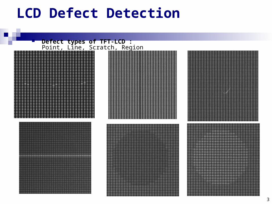
Defect types of TFT-LCD : Point, Line, Scratch, Region
LCD Defect Detection

4
Shading
Scanners give us raw point cloud data How to compute normals to shade the surface?
normal
5
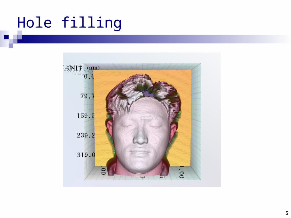
Hole filling

6
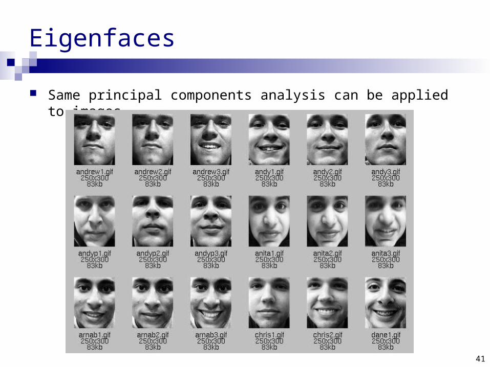
Eigenfaces
Same principal components analysis can be applied to images
7
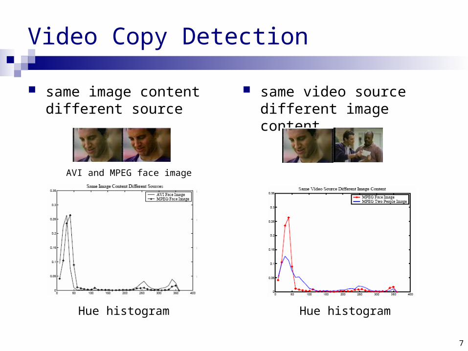
Video Copy Detection
same image content different source
same video source different image content
Hue histogram Hue histogram
AVI and MPEG face image

8
3D animations
Connectivity is usually constant (at least on large segments of the animation)
The geometry changes in each frame vast amount of data, huge filesize!
13 seconds, 3000 vertices/frame, 26 MB
9
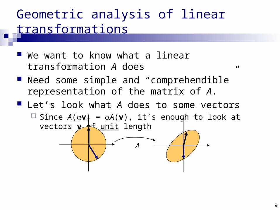
Geometric analysis of linear transformations
We want to know what a linear transformation A does Need some simple and “comprehendible” representation
of the matrix of A. Let’s look what A does to some vectors
Since A(v) = A(v), it’s enough to look at vectors v of unit length
A
10
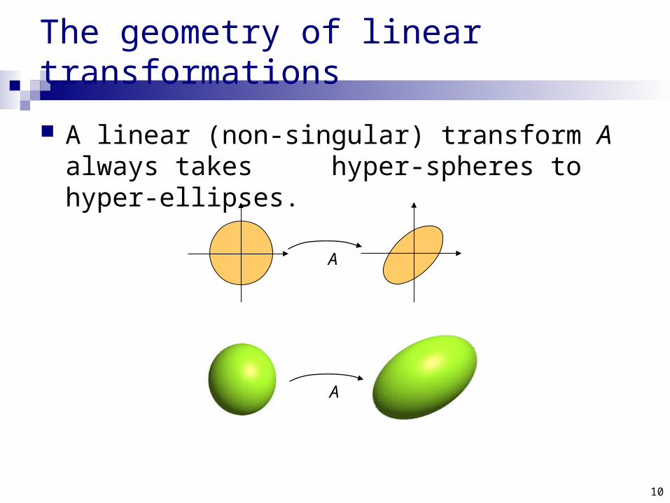
The geometry of linear transformations
A linear (non-singular) transform A always takes hyper-spheres to hyper-ellipses.
A
A
11
The geometry of linear transformations
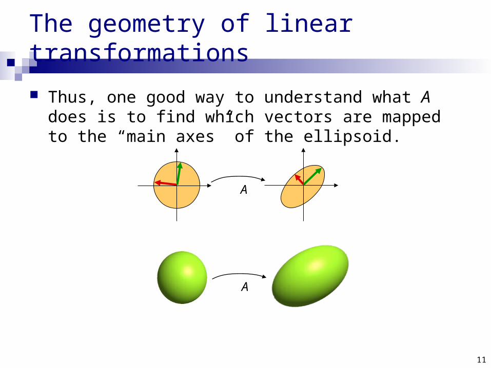
Thus, one good way to understand what A does is to find which vectors are mapped to the “main axes” of the ellipsoid.
A
A
12
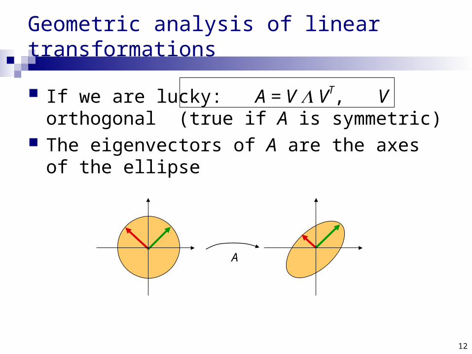
Geometric analysis of linear transformations
If we are lucky: A = V VT, V orthogonal (true if A is symmetric)
The eigenvectors of A are the axes of the ellipse
A
13
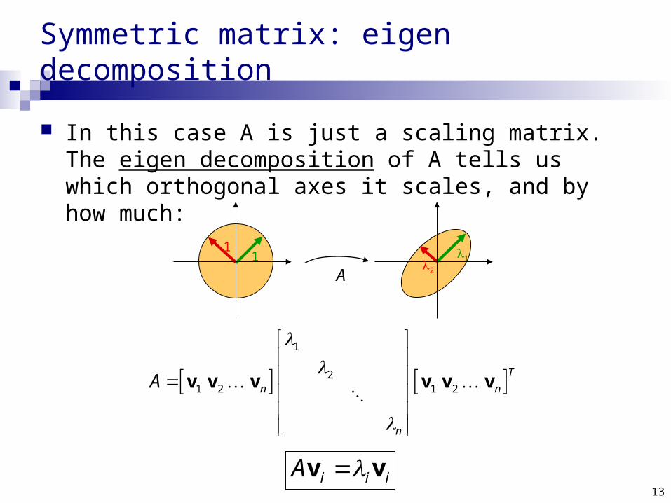
Symmetric matrix: eigen decomposition
In this case A is just a scaling matrix. The eigen decomposition of A tells us which orthogonal axes it scales, and by how much:
1
21 2 1 2
T
n n
n
A
v v v v v v
A
11
2
1
iiiA vv

14
General linear transformations: SVD
In general A will also contain rotations, not just scales:
A
1
21 2 1 2
T
n n
n
A
u u u v v v
1 1 2
1
TA U V

15
General linear transformations: SVD
A
1
21 2 1 2n n
n
A
v v v u u u
1 1 2
1
AV U
, 0i iA i iv u
orthonormal orthonormal

16
SVD more formally
SVD exists for any matrix Formal definition:
For square matrices A Rnn, there exist orthogonal matrices U, V Rnn and a diagonal matrix , such that all the diagonal values i of are non-negative and
TA U V
=
A U TV
17
SVD more formally
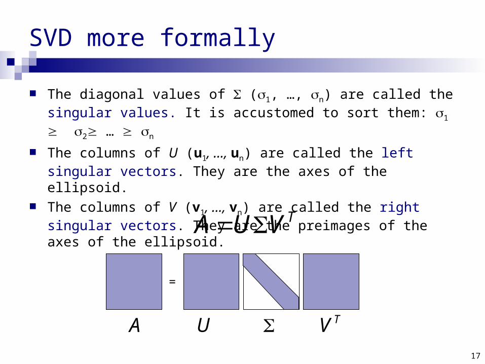
The diagonal values of (1, …, n) are called the singular values. It is accustomed to sort them: 1 2 … n
The columns of U (u1, …, un) are called the left singular vectors. They are the axes of the ellipsoid.
The columns of V (v1, …, vn) are called the right singular vectors. They are the preimages of the axes of the ellipsoid.
TA U V
=
A U TV
18
SVD is the “working horse” of linear algebra
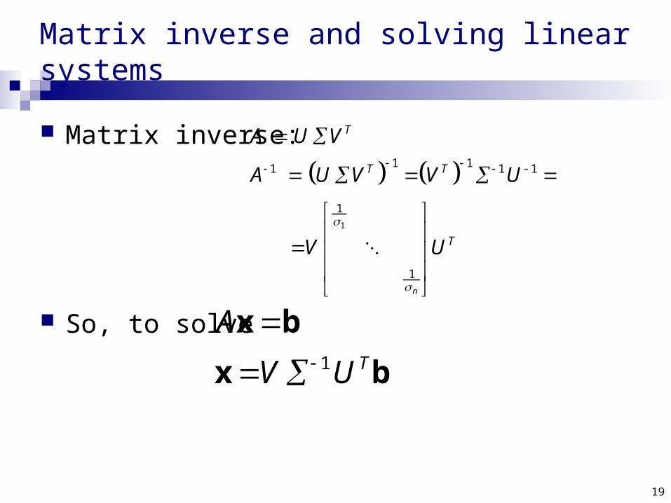
There are numerical algorithms to compute SVD. Once you have it, you have many things: Matrix inverse can solve square linear systems Numerical rank of a matrix Can solve least-squares systems PCA Many more…
19
Matrix inverse and solving linear systems
Matrix inverse:
So, to solve
1
1 11 1 1
1
1n
T
T T
T
A U V
A U V V U
V U
1 T
A
V U
x b
x b
20
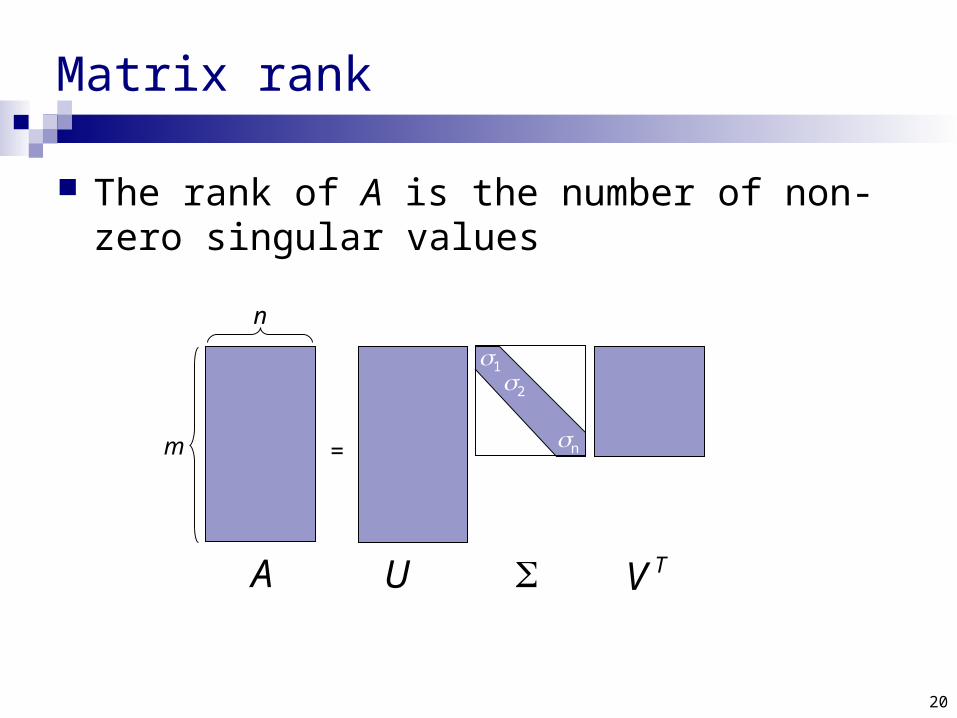
Matrix rank
The rank of A is the number of non-zero singular values
A U TV
=m
n
12
n
21
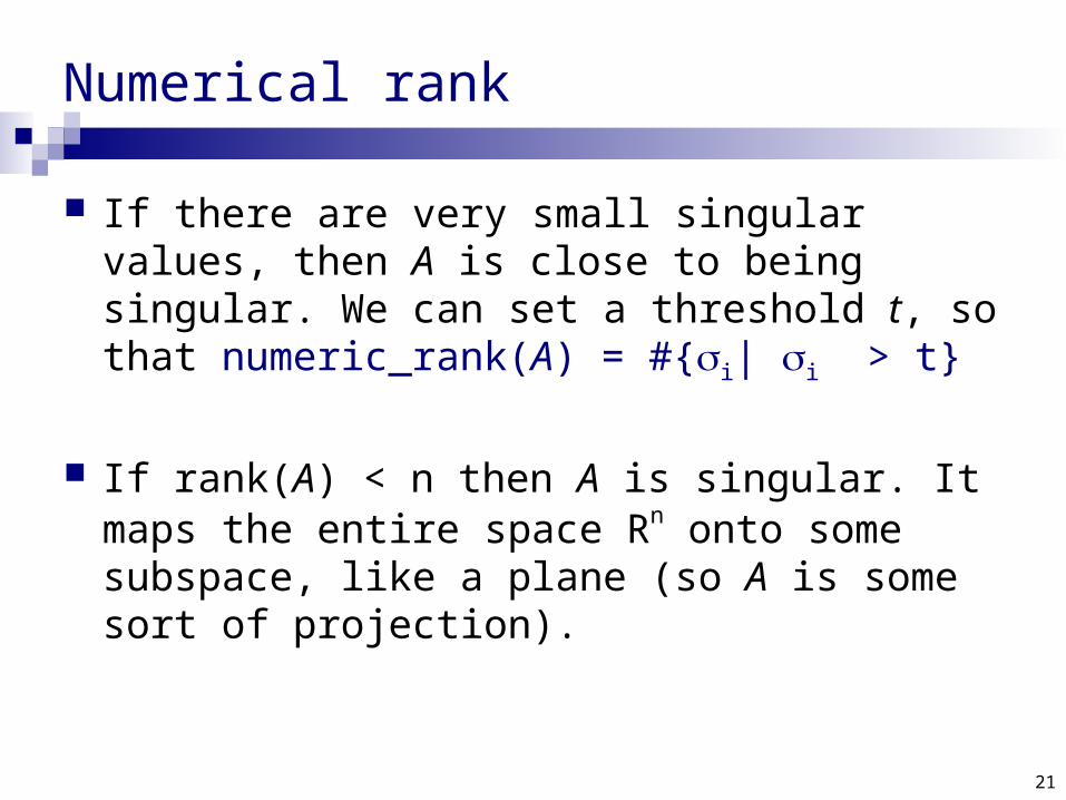
Numerical rank
If there are very small singular values, then A is close to being singular. We can set a threshold t, so that numeric_rank(A) = #{i| i > t}
If rank(A) < n then A is singular. It maps the entire space Rn onto some subspace, like a plane (so A is some sort of projection).
22
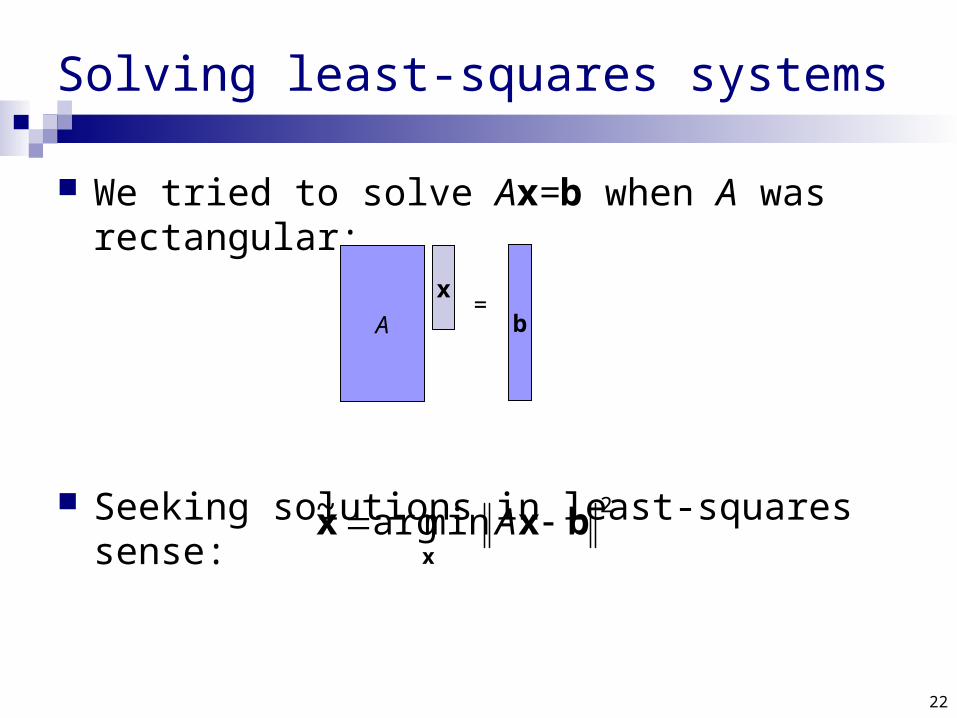
Solving least-squares systems
We tried to solve Ax=b when A was rectangular:
Seeking solutions in least-squares sense:2
minarg~ bxxx
A
A
x
b=
23
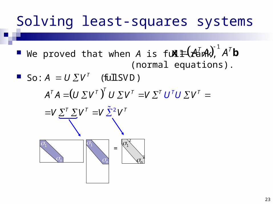
Solving least-squares systems
We proved that when A is full-rank, (normal equations).
So:
2
(full SVD)T
TT T T T T
T T
T
T
A U V
A A U V U V V V
V V V V
U U
1T TA A A
x b
=1
2
n2
1
n n
1
24
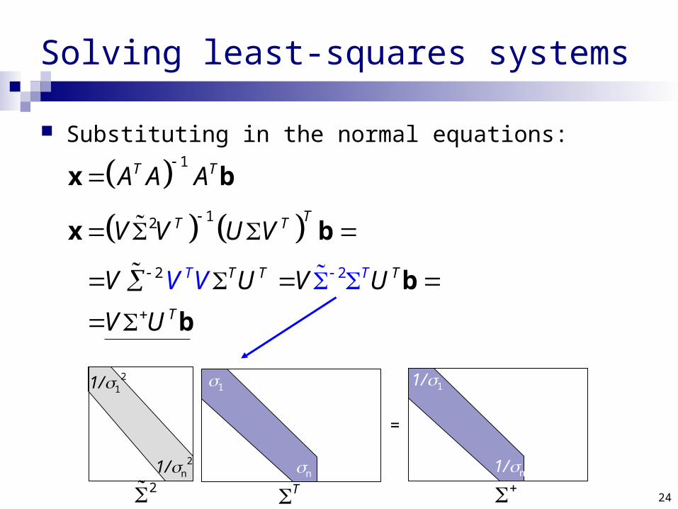
Solving least-squares systems
Substituting in the normal equations:
1
12
22
T T
TT T
T T TT
T
T
A A A
V V U V
V U V U
V
V V
U
x b
x b
b
b
1/12
1/n2
1
n
=
1/1
1/n
2 T
25
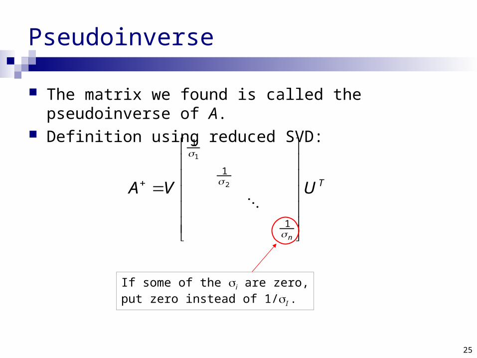
Pseudoinverse
The matrix we found is called the pseudoinverse of A. Definition using reduced SVD:
1
2
1
1
1n
TA V U
If some of the i are zero,put zero instead of 1/I .
26
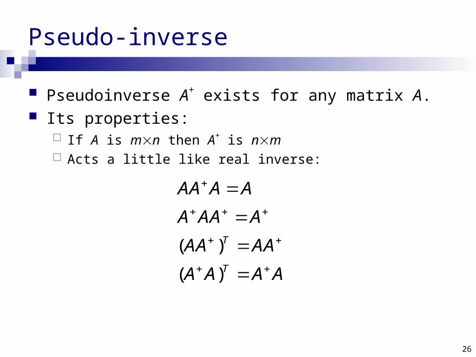
Pseudo-inverse
Pseudoinverse A+ exists for any matrix A. Its properties:
If A is mn then A+ is nm Acts a little like real inverse:
( )
( )
T
T
AA A A
A AA A
AA AA
A A A A
27
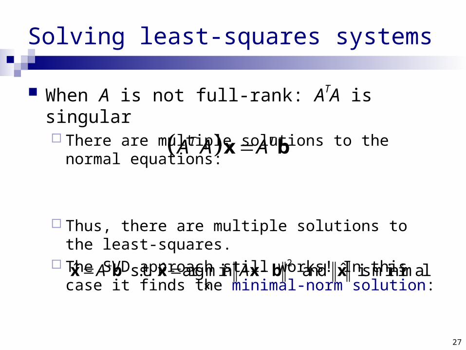
Solving least-squares systems
When A is not full-rank: ATA is singular There are multiple solutions to the normal equations:
Thus, there are multiple solutions to the least-squares.
The SVD approach still works! In this case it finds the minimal-norm solution:
2ˆ ˆ ˆs.t. arg min and is minimalA A x
x b x x b x
T TA A Ax b
28
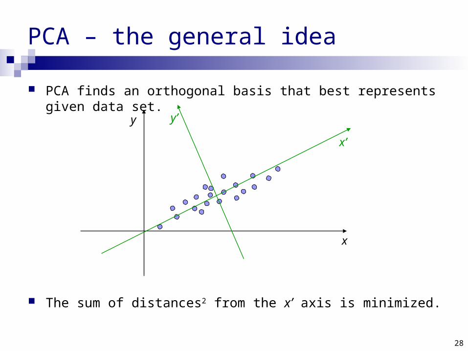
PCA finds an orthogonal basis that best represents given data set.
The sum of distances2 from the x’ axis is minimized.
PCA – the general idea
x
y
x’
y’
29
x
yv1
v2
x
y
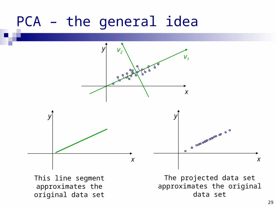
This line segment approximates the original data set
The projected data set approximates the original data set
x
y
PCA – the general idea
30
PCA – the general idea
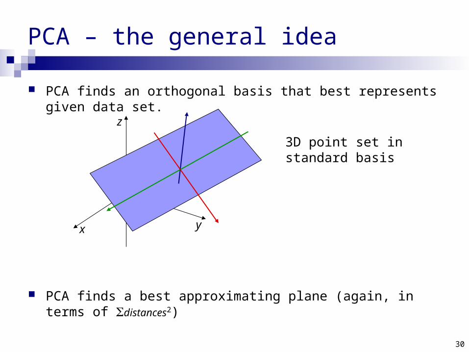
PCA finds an orthogonal basis that best represents given data set.
PCA finds a best approximating plane (again, in terms of distances2)
3D point set instandard basis
x y
z
31
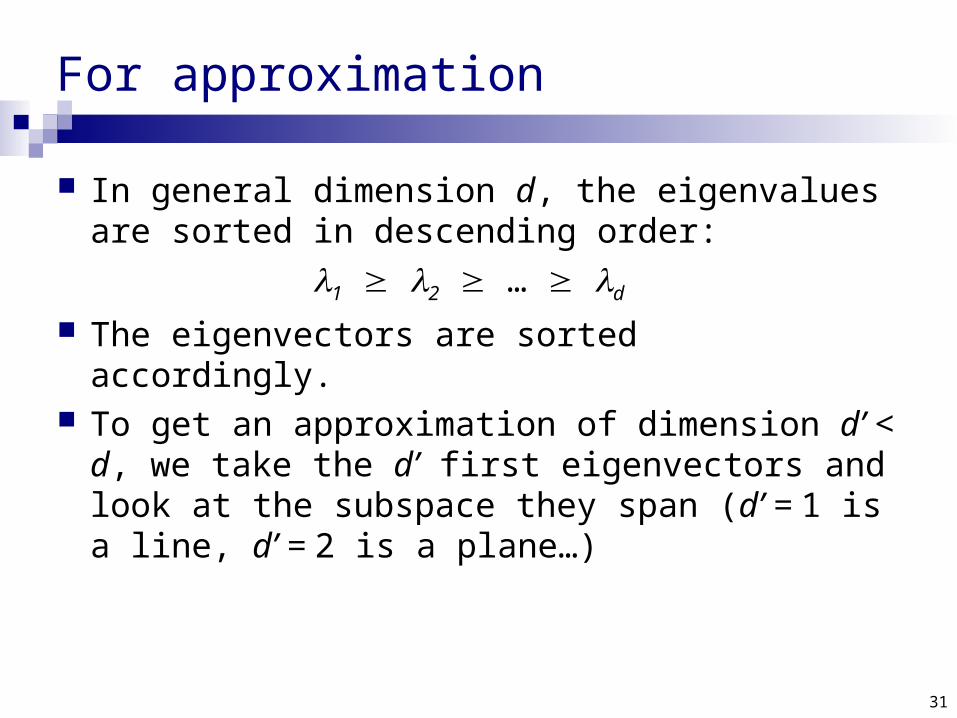
For approximation
In general dimension d, the eigenvalues are sorted in descending order:
1 2 … d The eigenvectors are sorted accordingly. To get an approximation of dimension d’ < d, we
take the d’ first eigenvectors and look at the subspace they span (d’ = 1 is a line, d’ = 2 is a plane…)
32
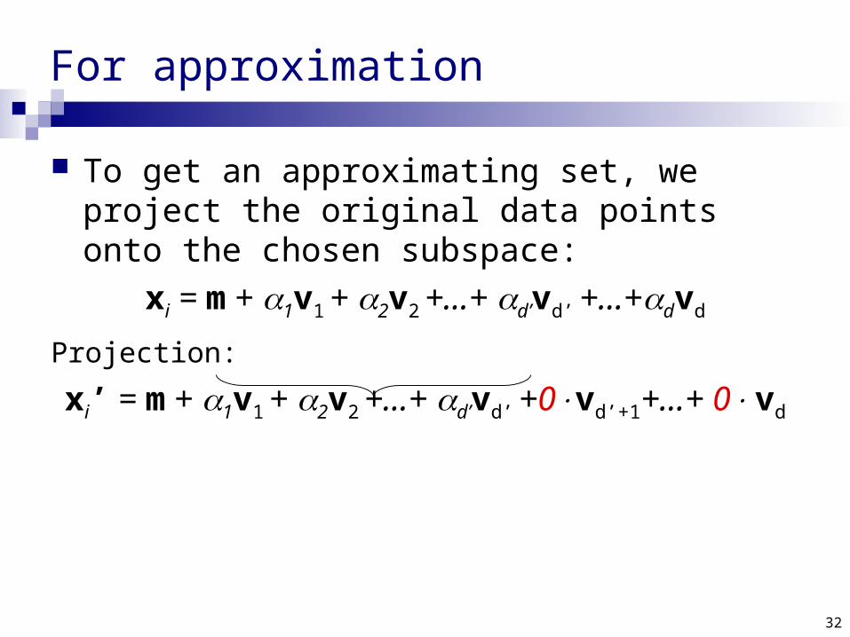
For approximation
To get an approximating set, we project the original data points onto the chosen subspace:
xi = m + 1v1 + 2v2 +…+ d’vd’ +…+dvd
Projection:
xi’ = m + 1v1 + 2v2 +…+ d’vd’ +0vd’+1+…+ 0 vd

33
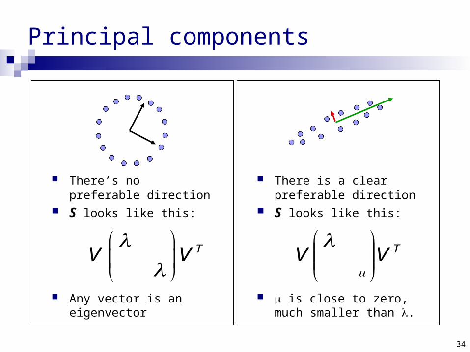
Principal components
Eigenvectors that correspond to big eigenvalues are the directions in which the data has strong components (= large variance).
If the eigenvalues are more or less the same – there is no preferable direction.
Note: the eigenvalues are always non-negative. Think why…
34
Principal components
There’s no preferable direction
S looks like this:
Any vector is an eigenvector
TV V
There is a clear preferable direction
S looks like this:
is close to zero, much smaller than .
TVV

35
Application: finding tight bounding box
An axis-aligned bounding box: agrees with the axes
x
y
minX maxX
maxY
minY
36
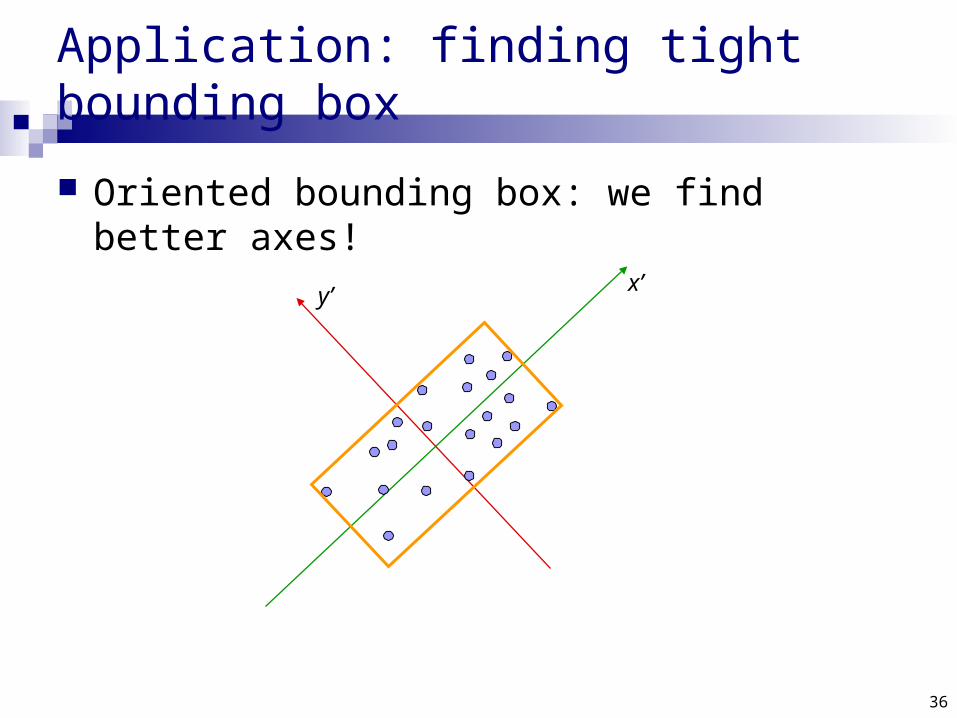
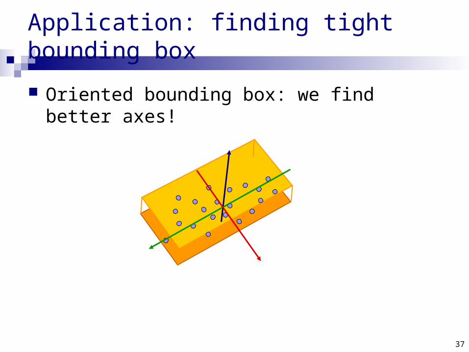
Application: finding tight bounding box
Oriented bounding box: we find better axes!
x’y’
37
Application: finding tight bounding box
Oriented bounding box: we find better axes!
38
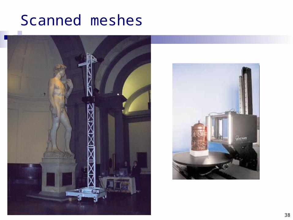
Scanned meshes
39
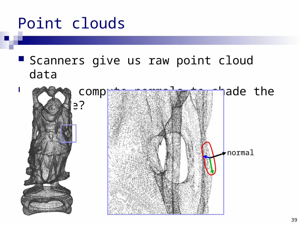
Point clouds
Scanners give us raw point cloud data How to compute normals to shade the surface?
normal
40
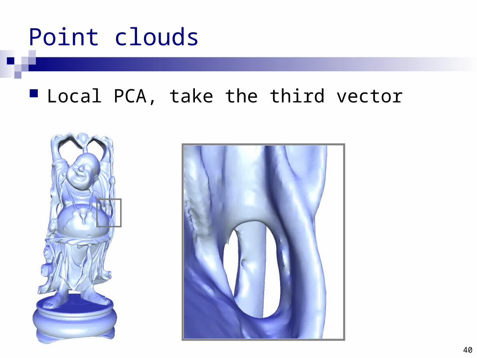
Point clouds
Local PCA, take the third vector
41
Eigenfaces
Same principal components analysis can be applied to images
42
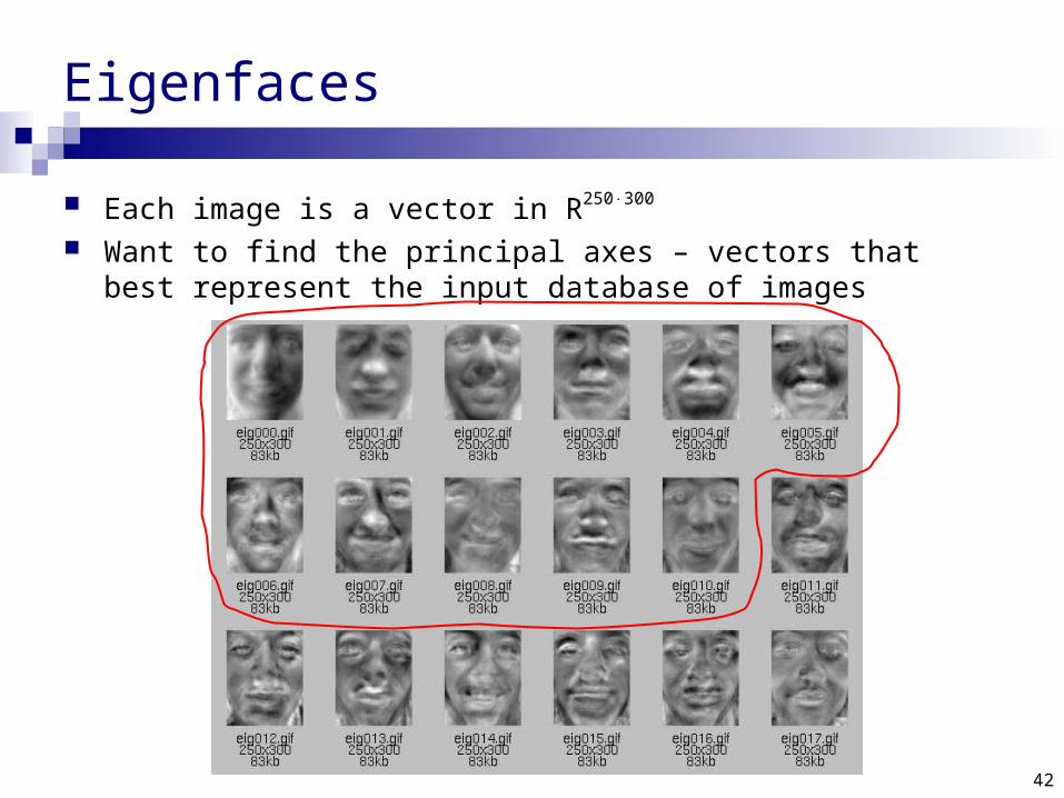
Eigenfaces
Each image is a vector in R250300
Want to find the principal axes – vectors that best represent the input database of images
43
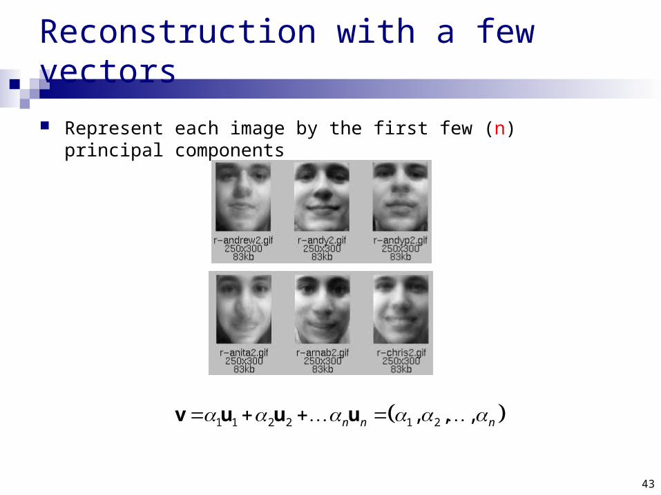
Reconstruction with a few vectors
Represent each image by the first few (n) principal components
1 1 2 2 1 2, , ,n n n v u u u
44
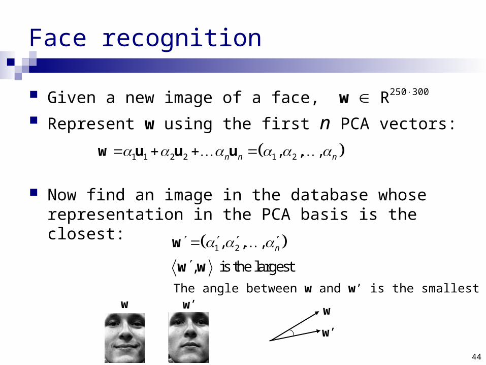
Face recognition
Given a new image of a face, w R250300
Represent w using the first n PCA vectors:
Now find an image in the database whose representation in the PCA basis is the closest:
1 1 2 2 1 2, , ,n n n w u u u
1 2, , ,
, is the largest
n
w
w w
The angle between w and w’ is the smallestw w’
w’
w
45
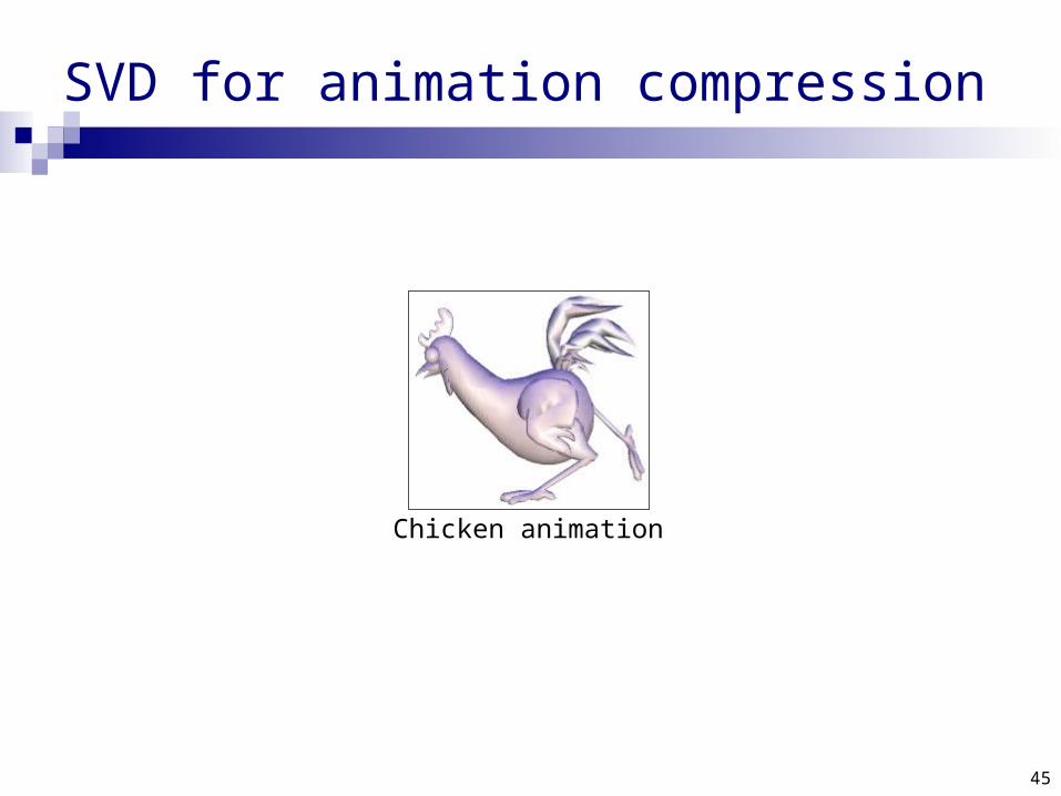
SVD for animation compression
Chicken animation
46
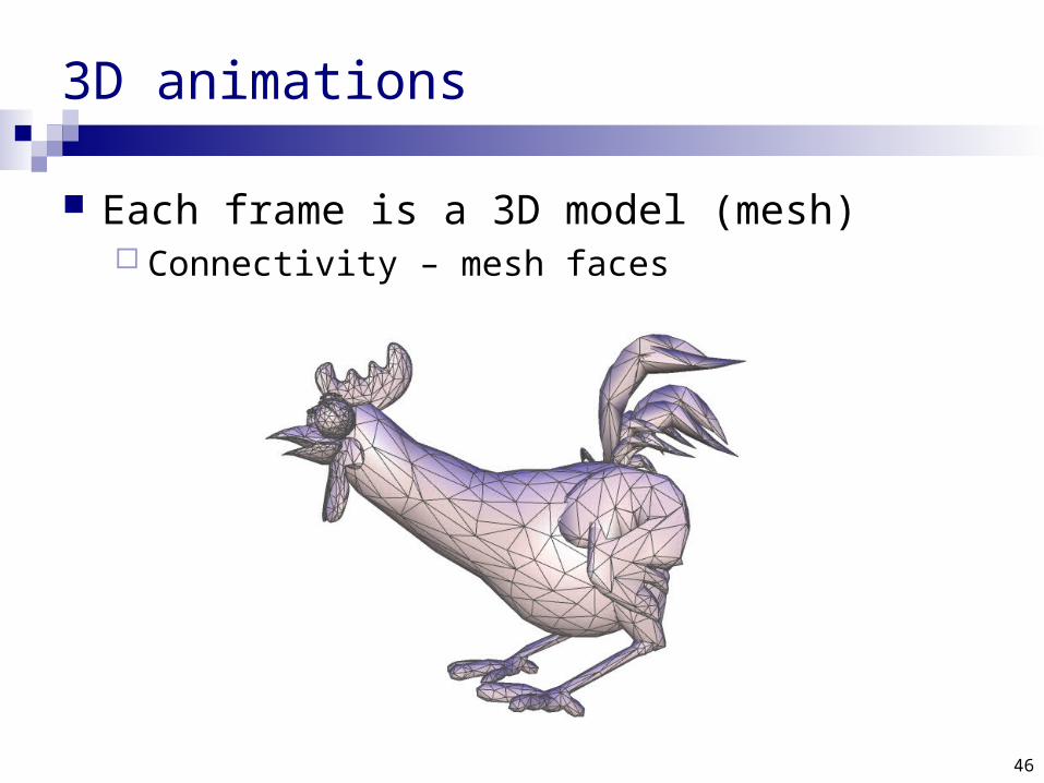
3D animations
Each frame is a 3D model (mesh) Connectivity – mesh faces

47
3D animations
Each frame is a 3D model (mesh) Connectivity – mesh faces Geometry – 3D coordinates of the vertices

48
3D animations
Connectivity is usually constant (at least on large segments of the animation)
The geometry changes in each frame vast amount of data, huge filesize!
13 seconds, 3000 vertices/frame, 26 MB
49
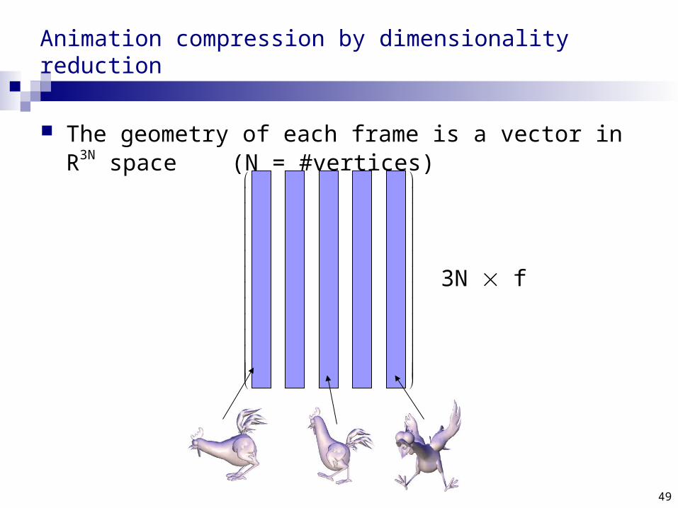
Animation compression by dimensionality reduction
The geometry of each frame is a vector in R3N space (N = #vertices)
1
1
1
N
N
N
x
x
y
y
z
z
3N f
50
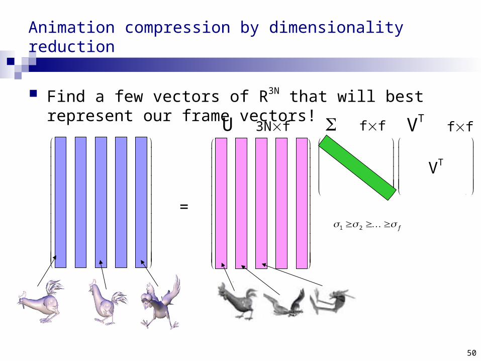
Animation compression by dimensionality reduction
Find a few vectors of R3N that will best represent our frame vectors!
1
1
1
N
N
N
x
x
y
y
z
z
=
1
2
f
1
2
f
VT
U 3Nf ff VT ff
1 2 f
51
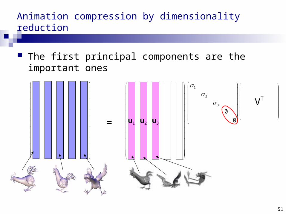
Animation compression by dimensionality reduction
The first principal components are the important ones
1
1
1
N
N
N
x
x
y
y
z
z
=
u1 u2 u3
1
2
f
VT
1
2
3
0
0
52
1
1
1
N
N
N
x
x
y
y
z
z
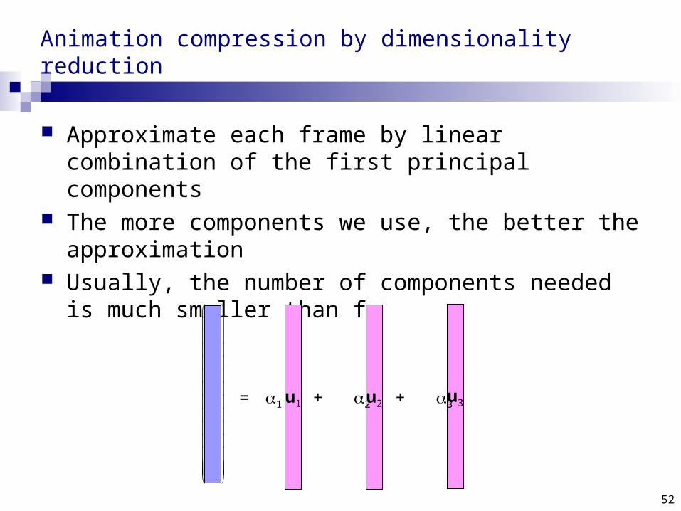
Animation compression by dimensionality reduction
Approximate each frame by linear combination of the first principal components
The more components we use, the better the approximation
Usually, the number of components needed is much smaller than f.
= u1 u2 u31 + 2 + 3
53
Animation compression by dimensionality reduction
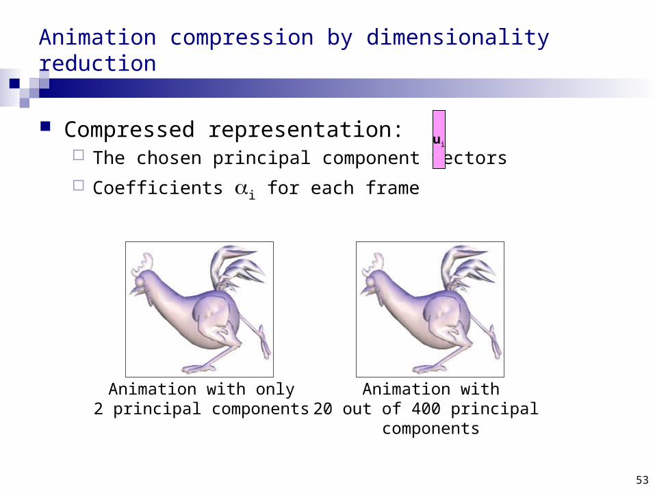
Compressed representation: The chosen principal component vectors
Coefficients i for each frame
ui
Animation with only2 principal components
Animation with20 out of 400 principal
components

54
Defect types of TFT-LCD : Point, Line, Scratch, Region
LCD Defect Detection
55
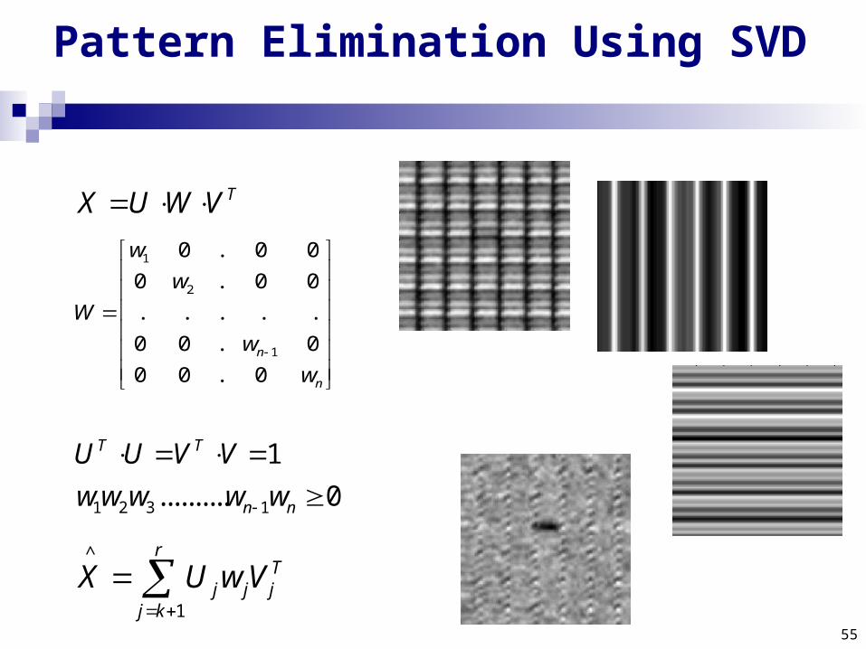
1
2
1
0 . 0 0
0 . 0 0
. . . . .
0 0 . 0
0 0 . 0n
n
w
w
W
w
w
^
1
rT
j j jj k
X U w V
TX U W V
1 2 3 1
1
.......... 0
T T
n n
U U V V
w w w w w
Pattern Elimination Using SVD
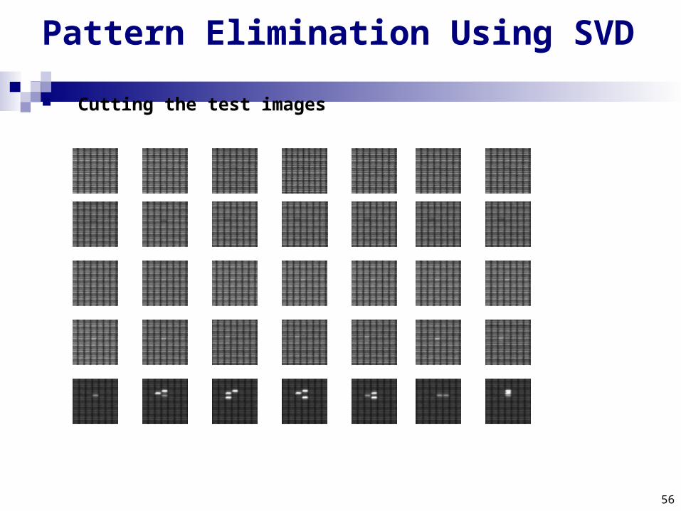
56
Cutting the test images
Pattern Elimination Using SVD
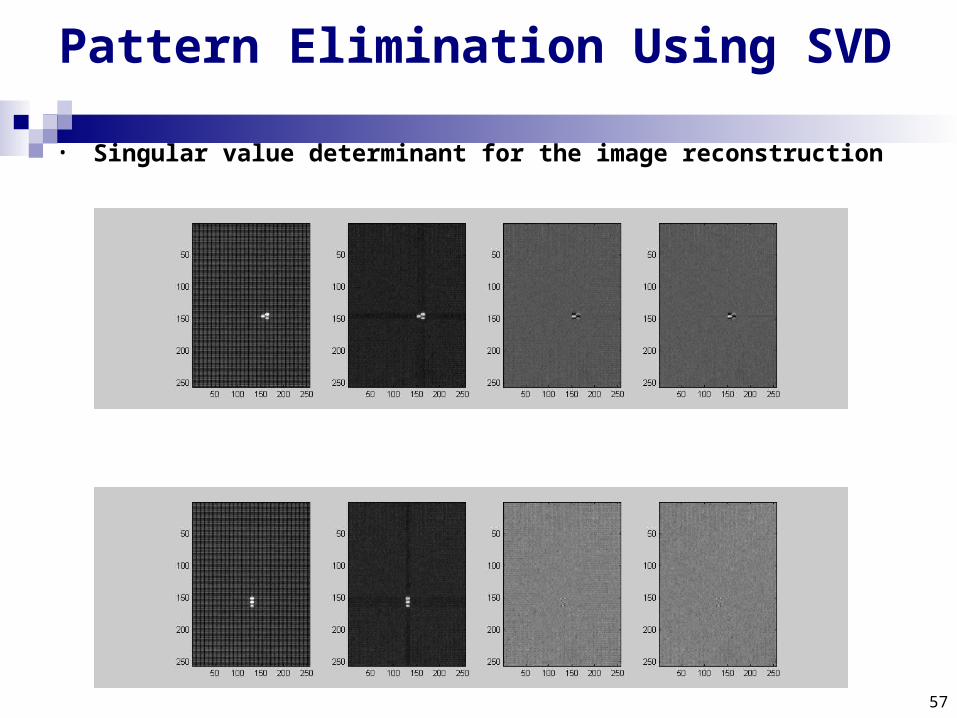
57
• Singular value determinant for the image reconstruction
Pattern Elimination Using SVD
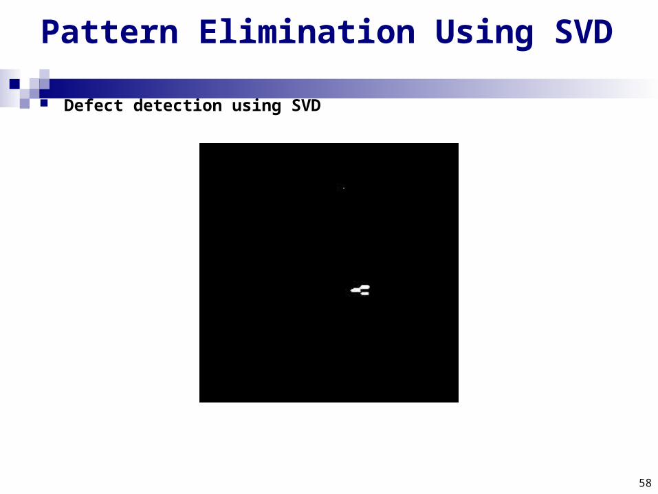
58
Defect detection using SVD
Pattern Elimination Using SVD