Synchronizing IEC 61850-9-2 withLegacy Real-time Embedded

Systems

DIPLOMA THESIS

submitted in partial fulfillment of the requirements for the degree of

Diplom-Ingenieur

in

Embedded Systems

by

Mario PETER, BScRegistration Number 01327117

to the Faculty of Electrical Engineering and IT

at the TU Wien

Advisor: Ao.Univ.Prof. Dipl.-Ing. Dr.techn. Thilo SAUTER

Vienna, 23rd September, 2021Mario PETER Thilo SAUTER

Technische Universität WienA-1040 Wien Karlsplatz 13 Tel. +43-1-58801-0 www.tuwien.at

Danksagung

An dieser Stelle möchte ich mich bei all jenen Personen recht herzlich bedanken, diemich während meines Studiums und dem Schreiben dieser Diplomarbeit unterstützt undmotiviert haben.

Zuerst gebührt mein Dank Herrn Ao.Univ.Prof. Dipl.-Ing. Dr.techn. Thilo SAUTER,der diese Arbeit betreut und begutachtet hat. Weiters möchte ich mich bei der FirmaOMICRON electronics GmbH1 und insbesondere bei meinen firmenseitigen BetreuernHerrn Dipl.-Ing. Tilman TRÄXLER und Herrn Domen SELINEC, MSc recht herz-lich bedanken, da sie mir die Möglichkeit gegeben haben, diese Industrie-Diplomarbeitdurchzuführen.

Neben den Betreuern möchte ich mich auch noch bei meinen Freunden und Studienkollegenbedanken, die mir bei Fragen oder Unklarheiten geholfen haben.

Abschließend möchte ich mich bei meinen Eltern bedanken, die mir mein Studiumermöglicht haben und stets ein offenes Ohr für meine Sorgen hatten.

1https://www.omicronenergy.com/de/

iii

Acknowledgements

At this point I would like to thank all those peoples who supported and motivated meduring my studies and the writing of this diploma thesis.

First, my thanks go to Mr. Ao.Univ.Prof. Dipl.-Ing. Dr.techn. Thilo SAUTER, whohas supervised and reviewed this work. Furthermore, I would like to thank the companyOMICRON electronics GmbH2 and in particular my company advisers Mr. Dipl.-Ing.Tilman TRÄXLER and Mr. Domen SELINEC, MSc because they gave me the opportunityto do this industrial diploma thesis.

In addition to the caregivers, I would also like to thank my friends and colleges fromuniversity that have helped me with questions or ambiguities.

Finally, I would like to thank my parents, who made my studies possible and always hadan open ear for my worries.

2https://www.omicronenergy.com/en/

v

Kurzfassung

Die elektrische Infrastruktur lässt sich in zwei Bereiche aufteilen. Der erste Bereich istdie Primärtechnik. Diese umfasst alle Schaltanlagen, die unmittelbar an der Erzeugung,dem Transport und der Verteilung elektrischer Energie beteiligt sind. Somit beinhaltetdie Primärtechnik beispielsweise Generatoren, Transformatoren, Schaltgeräte, Sammel-schienen und Leitungen. Neben der Primärtechnik gibt es ergänzend dazu auch noch dieSekundärtechnik. Dieser Bereich beinhaltet sämtliche Hilfseinrichtungen zur Messung,Überwachung, Kommunikation, Automatisierung und Fernsteuerung. Die Verbindungder zwei Bereiche wird über Messwandler und Leistungsschalter realisiert.

Wie in fast allen anderen Bereichen und Branchen durchläuft auch die elektrische In-frastruktur einen Digitalisierungsprozess. In dieser Diplomarbeit wird der Fokus aufdie Digitalisierung der Messwandler gelegt. Der Begriff Messwandler umfasst Strom-wandler (Current Transformers (CTs)) und Spannungswandler (Voltage Transformers(VTs)). Durch diese Änderung wird die Norm International Electrotechnical Commission(IEC) 61850 sehr wichtig. Für diese Diplomarbeit ist besonders der Bereich über Transportvon Sampled Values (SVs) über Ethernet-Netzwerke interessant, welcher im IEC 61850-9-2zu finden ist. Dieses Kapitel ist von Bedeutung, da es bei unkonventionellen Wandlerkeine Möglichkeit gibt die Sekundärseite analog zu messen, sondern nur noch über dieSVs, welche über die standardisierte Bus-Schnittstelle zur Verfügung gestellt werden.

Die Messwandler können weiterhin mit einem analogen Signal auf der Primärseite gespeistwerden, jedoch kann die Antwort des Messwandlers nur noch durch das Konsumierenund Interpretieren des SV-Streams erreicht werden. Die SVs werden mit einer von erNetzfrequenz abhängigen Abtastrate generiert und dann übers Netzwerk verteilt. Bei einerNetzfrequenz von 50 Hz ist die Abtastrate 4000 Hz und 4800 Hz bei einer Netzfrequenzvon 60 Hz. In dieser Diplomarbeit wird ein solcher SV-Stream von einem existierendenEchtzeit-Embedded-System konsumiert, wobei das System mit einer nicht veränderbarenSystemfrequenz getaktet ist, die sich von der Abtastrate der SVs unterscheidet. Inunserem Fall ist das System mit 10 kHz getaktet und daher wird in dieser Diplomarbeiteine Möglichkeit aufgezeigt, wie man diese SVs in das vorhandene Echtzeit-Embedded-System integrieren kann.

Damit das System die empfangenen SVs konsumieren und interpretieren kann, müssendiese ebenfalls auf eine Abtastrate von 10 kHz transformiert werden. Mit Hilfe derKubische Spline Interpolation wird die Abtastrate des empfangenen digitalen Signals

vii

auf ein Vielfaches der Systemfrequenz erhöht. Anschließend werden die nicht benötigtenAbtastwerte wieder entfernt, damit man am Ende eine Abtastrate von 10 kHz erreicht.Dieses transformierte Signal kann dann von der Echtzeitanwendung verwendet werden,um diverse Berechnungen durchzuführen.

In dieser Diplomarbeit konnte aufgezeigt werden, dass die gezeigte Implementierung keinenEinfluss auf das existierende Echtzeit-Embedded-System hat. Weiters wird gezeigt, dassder Fehler, der durch die Transformation des Signals entsteht, in einem sehr guten Bereichliegt und für die Anwendung ausreichend ist. Aufgrund der begrenzten Rechenleistung desSystems und der bereits hohen Auslastung der Echtzeitanwendung konnte die Evaluierungnur mit einem von acht Kanälen des SV-Streams durchgeführt werden. Die vorgestellteLösung kann aber jederzeit erweitert werden, damit alle empfangenen Ströme undSpannungen transformiert und verwendet werden können.

Abstract

The electrical infrastructure can be divided into two areas. The first area is primarytechnology. This includes all switchgears that are directly involved in the generation,transport and distribution of electrical energy. Thus, the primary technology includesfor example generators, transformers, switching devices, busbars and cables. In additionto the primary technology there is also the secondary technology. This area containsall auxiliary equipment for measurement, monitoring, communication, automation andremote control. The connection between the two areas is implemented using instrumenttransformers and circuit breakers.

As in almost all other areas and industries the electrical infrastructure is also going througha digitization process. In this diploma thesis the focus is placed on the digitization of theinstrument transformers. The term measuring transformer includes Current Transformers(CTs) and Voltage Transformers (VTs). With this change a standard of the InternationalElectrotechnical Commission (IEC) becomes very important. The mentioned standard isIEC 61850. For this diploma thesis the area about the transport of Sampled Values (SVs)over Ethernet networks is particularly interesting, which can be found in IEC 61850-9-2.This chapter is important because with Non-Conventional Instrument Transformers(NCIT) there is no possibility to measure the secondary side analogously, but only viathe SVs, which are made available via the standardized bus interface.

This diploma thesis shows how this SVs can be integrated into an existing real-timeembedded system that works with a specific and unchangeable system frequency. Inthis special case Ethernet for Control Automation Technology (EtherCAT) specifiesthe frequency, which is for the used system a frequency of 10 kHz. Since the SVs arereceived at a different frequency, an interface has to be created that transforms this SVsto the given system frequency. This data can only be used if the received SVs have beensynchronized to the system frequency. Otherwise, there is no relationship between themeasuring signals and the received result data.

ix

Contents

Kurzfassung vii

Abstract ix

Contents xi

1 Introduction 11.1 Problem Statement . . . . . . . . . . . . . . . . . . . . . . . . . . . . . . 11.2 Aim of the Thesis . . . . . . . . . . . . . . . . . . . . . . . . . . . . . . 41.3 Structure of the Thesis . . . . . . . . . . . . . . . . . . . . . . . . . . . 5

2 Background 72.1 Electric power system . . . . . . . . . . . . . . . . . . . . . . . . . . . 72.2 IEC 61850 - Communication networks and systems for power utility

automation . . . . . . . . . . . . . . . . . . . . . . . . . . . . . . . . . 92.2.1 IEC 61850-9-2 . . . . . . . . . . . . . . . . . . . . . . . . . . . 122.2.2 IEC 61850-9-2-LE . . . . . . . . . . . . . . . . . . . . . . . . . 13

2.3 IEEE 1588 . . . . . . . . . . . . . . . . . . . . . . . . . . . . . . . . . . 132.4 EtherCAT . . . . . . . . . . . . . . . . . . . . . . . . . . . . . . . . . . 152.5 Measuring device - TESTRANO 600 . . . . . . . . . . . . . . . . . . . 18

3 Related Work 23

4 Implementation 294.1 Resample . . . . . . . . . . . . . . . . . . . . . . . . . . . . . . . . . . 29

4.1.1 Upsampling . . . . . . . . . . . . . . . . . . . . . . . . . . . . . 304.1.2 Selection of a suitable algorithm . . . . . . . . . . . . . . . . . 324.1.3 Spline interpolation . . . . . . . . . . . . . . . . . . . . . . . . 344.1.4 Downsampling/Decimation . . . . . . . . . . . . . . . . . . . . 38

4.2 Bridge . . . . . . . . . . . . . . . . . . . . . . . . . . . . . . . . . . . . 45

5 Evaluation 495.1 Evaluation setup . . . . . . . . . . . . . . . . . . . . . . . . . . . . . . 495.2 Network traffic analysis . . . . . . . . . . . . . . . . . . . . . . . . . . . 51

xi

5.3 Packet timing analysis . . . . . . . . . . . . . . . . . . . . . . . . . . . 525.4 Analysis of the output and input signals . . . . . . . . . . . . . . . . . 535.5 Analysis of real-time behaviour . . . . . . . . . . . . . . . . . . . . . . 58

6 Conclusion and Future Work 61

A IEC 61850 Parts 63

B Content of an IEC 61850-9-2-LE Ethernet frame 65

C Content of the additional ET 2000 packet data 69

List of Figures 71

List of Tables 73

List of Algorithms 75

Acronyms 77

Bibliography 81

CHAPTER 1Introduction

1.1 Problem StatementAs in almost all other areas and industries, the electrical infrastructure is also goingthrough a digitization process. Through this digitization, the conventional instrumenttransformers (including Current Transformers (CTs) and Voltage Transformers (VTs))are replaced by so called Non-Conventional Instrument Transformers (NCIT), whichhave only digital output signals on the secondary side of the transformer and no analogoutputs anymore. Therefore, the measurement methods also have to be adapted to thenew situation.

These NCIT are more frequently used not only because of digitization, which is currentlythe trend, but also because they operate in non-conventional ways. One example of thisis that NCIT sometimes also use optical technology and thus have some advantages overconventional transformers [TNT+97]. For example a fiber optic cable is used as a sensorand is mounted around the conductor to measure the current. This is done based onthe Faraday effect. This effect describes the rotation of the plane of polarization of alight beam by a magnetic field [CXW20]. Another reason for using NCIT is that theyare capable of higher voltages and currents while still being as compact as possible. Inorder to achieve this compactness, the transformers must be isolated with a special gasand then can not simply be broken up to make a measurement [TNT+97].

Therefore, the standard International Electrotechnical Commission (IEC) 61850 on“Communication Networks and Systems in Substation” becomes an important topicwhich defines communication protocols, data formats and the configuration language forIntelligent Electronic Devices (IEDs) at electrical substations. All parts of the standardare listed in Table A.1. For this thesis the subsection IEC 61850-9-2 is the most relevantone and defines the protocol how Sampled Values (SVs) shall be transmitted over anEthernet network. In this context, SVs are discrete samples of the voltages and currents

1

1. Introduction

of the transformer. So all analog voltages and currents are sampled with a defined samplerate and these samples are summarized in the SV packet with the associated phases andstatus information and then transmitted over the network.

With this digital interface we face now the situation that the transformers on the primaryside can still be excited with an analog signal, but there are no analog ports on thesecondary side to measure the response analogously. We only have the possibility toconsume the generated SVs and thus receive the response of the transformer. Thevalues of the secondary side are very important, since many of the test methods usedin asset diagnostics allow a conclusion only with this data and in combination with themeasuring signal on the primary side. Such a measurement is for example to measurethe transmission accuracy or the phase shift error of the transformer or to identify shortwindings on instrument transformers by measuring the transformation ratio [PFA17].

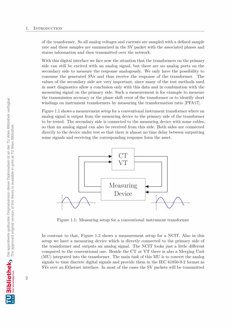
Figure 1.1 shows a measurement setup for a conventional instrument transformer where ananalog signal is output from the measuring device to the primary side of the transformerto be tested. The secondary side is connected to the measuring device with some cables,so that an analog signal can also be received from this side. Both sides are connecteddirectly to the device under test so that there is almost no time delay between outputtingsome signals and receiving the corresponding response form the asset.

MeasuringDevice

CTVT

Figure 1.1: Measuring setup for a conventional instrument transformer

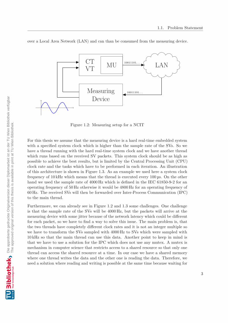
In contrast to that, Figure 1.2 shows a measurement setup for a NCIT. Also in thissetup we have a measuring device which is directly connected to the primary side ofthe transformer and outputs an analog signal. The NCIT looks just a little differentcompared to the conventional one. Beside the CT or VT there is also a Merging Unit(MU) integrated into the transformer. The main task of this MU is to convert the analogsignals to time discrete digital signals and provide them in the IEC 61850-9-2 format asSVs over an Ethernet interface. In most of the cases the SV packets will be transmitted

2

1.1. Problem Statement

over a Local Area Network (LAN) and can than be consumed from the measuring device.

MeasuringDevice

CTVT MU LAN10011101. . .

10011101. . .

Figure 1.2: Measuring setup for a NCIT

For this thesis we assume that the measuring device is a hard real-time embedded systemwith a specified system clock which is higher than the sample rate of the SVs. So wehave a thread running with the hard real-time system clock and we have another threadwhich runs based on the received SV packets. This system clock should be as high aspossible to achieve the best results, but is limited by the Central Processing Unit (CPU)clock rate and the tasks which have to be performed in each iteration. An illustrationof this architecture is shown in Figure 1.3. As an example we used here a system clockfrequency of 10 kHz which means that the thread is executed every 100 µs. On the otherhand we used the sample rate of 4000 Hz which is defined in the IEC 61850-9-2 for anoperating frequency of 50 Hz otherwise it would be 4800 Hz for an operating frequency of60 Hz. The received SVs will then be forwarded over Inter-Process Communication (IPC)to the main thread.

Furthermore, we can already see in Figure 1.2 and 1.3 some challenges. One challengeis that the sample rate of the SVs will be 4000 Hz, but the packets will arrive at themeasuring device with some jitter because of the network latency which could be differentfor each packet, so we have to find a way to solve this issue. The main problem is, thatthe two threads have completely different clock rates and it is not an integer multiple sowe have to transform the SVs sampled with 4000 Hz to SVs which were sampled with10 kHz so that the main thread can use this data. Another point to keep in mind isthat we have to use a solution for the IPC which does not use any mutex. A mutex ismechanism in computer science that restricts access to a shared resource so that only onethread can access the shared resource at a time. In our case we have a shared memorywhere one thread writes the data and the other one is reading the data. Therefore, weneed a solution where reading and writing is possible at the same time because waiting for

3

1. Introduction

Measuring device

Thread 1

=100 µs(10 kHz)

Thread 2

=250 µs(4000 Hz)

IPC

Figure 1.3: Thread overview of the measuring device

the mutex to be released from the other thread could break the hard real-time conditionbecause the main thread has no time left for waiting. Nevertheless, thread safety mustbe guaranteed at all times, even without using a mutex.

Another important point is that the NCIT is connected to a high accuracy time sourceso that the signals can be sampled with a high precision resulting in equidistant samples.In the past a 1 Pulse Per Second (PPS) signal was used to synchronize the local runningclock on the device. Over time the 1PPS signal was replaced by the Institute of Electricaland Electronics Engineers (IEEE) 1588 protocol which can be used to time synchronizemultiple devices over Ethernet [SNKB19]. Therefore, it is mandatory that the measuringdevice can also receive the IEEE 1588 packets and can synchronize the local time to thetime information provided form the Precision Time Protocol (PTP) grandmaster clock.In our case the grandmaster provides a Global Positioning System (GPS) controlled timereference and distributes this time information to the measuring device as well as to theintegrated MU of the device to be tested.

A last point to consider is that the solution will be implemented and evaluated on a hardreal-time embedded system with limited resources and computation power. Therefore,the solutions should not be too complex and be as resource efficient as possible so thatthe already running hard real-time system does not get disturbed.

1.2 Aim of the ThesisThe aim of this thesis is to provide some background information about the related topicsand the different standards, which are parts of this problem. Another goal of this thesisis to deal with the time jitter of the received SVs which is caused by the network. Themain intention is to find a time and resource efficient solution to exchange sample databetween two threads which are running on completely different clock frequencies. A

4

1.3. Structure of the Thesis

practical implementation should be based on a commercial off the shelf IPC architecture.Therefore, we need a smart solution to use shared memory without using any kind ofmutual exclusion mechanism because the hard real-time system has no time left forwaiting to access a shared resource. For performance evaluation, an existing measuringdevice should be extended with this solution and evaluate what is possible and whatrestrictions the implementation has on the test device. An important point here is thatthe already existing hard real-time embedded system works as before and is not disturbedby the solution of this thesis. The last aim of this thesis is to evaluate the implementationon the measuring device and compare the results with expected results from differentsimulations and check the timing behaviour of the system.

1.3 Structure of the ThesisThe remainder of this thesis is structured as follows. Chapter 2 provides the reader withhelpful background information related to the topic of this thesis. General terms in thefield of power supply systems are explained and in Section 2.2 and 2.3 the necessarystandards are specifically addressed and explained. In Section 2.5 the measuring deviceis described in detail, which was used to implement and evaluate the solution.

In the next Chapter 3 we provide an overview about existing state-of-the-art approachesto resampling and synchronization of two threads with different iteration cycle times.

The implementation of the resampling algorithm and the bridge between the SV-systemand the Ethernet for Control Automation Technology (EtherCAT)-master is documentedin Chapter 4.

Chapter 5 provides the evaluation of the existing embedded system with the synchroniza-tion to the SV-system.

Finally, in Chapter 6 the thesis is concluded with a summary of the presented work andgive an outlook on future work.

5

CHAPTER 2Background

2.1 Electric power systemIn 1882, the first power station was commissioned in New York City. The power industrygrew very fast and generation stations and transmission and distribution networks spreadall over the country [Gö14].

The main tasks of an electrical power system are to generate, transmit and distributeelectrical energy efficiently. In electric power systems, generators produce the energy asneeded. They are therefore not storage systems such as water or gas systems [Blu07].

A power system can be divided into two major infrastructures. On the one hand it isthe power grid and on the other the communication system. The power grid will bedescribed in the next paragraph and the communication system will be described in thenext Section 2.2 [SW05].

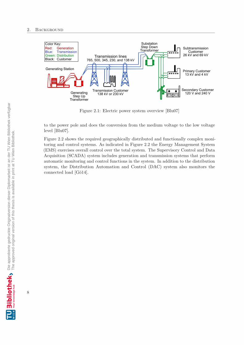
Figure 2.1 shows the different stations from power generation to the consumer. It is asimplified power system, but the basic principles, concepts, theories and terminologies arethe same. On the left side of the image the power generation in the power plant is shownas a first step. The power plants convert energy sources into electrical energy. Such energysources are, for example, heat, mechanical, hydraulic, chemical, solar, wind, geothermal,nuclear and other energy sources. Subsequently, this electrical energy is converted atthe power station into high-voltage electrical energy, as this is better suited for efficientlong-distance transport. The next part is the high-voltage transmission lines, whichefficiently transport electrical energy over long distances to the consumption locations. Atthe end of the high-voltage lines are substations, which convert the electrical high-voltageinto a medium-voltage. Subsequently, this medium-voltage energy is transmitted viadistribution power lines and can be directly connected to primary customers such asbigger industries. Last but not least, the energy is converted once more close to thesecondary customer to the low-voltage level. In Figure 2.1 the transformer is attached

7

2. Background

Figure 2.1: Electric power system overview [Blu07]

to the power pole and does the conversion from the medium voltage to the low voltagelevel [Blu07].

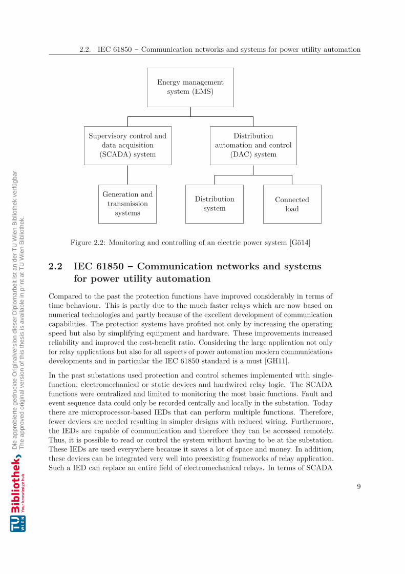
Figure 2.2 shows the required geographically distributed and functionally complex moni-toring and control systems. As indicated in Figure 2.2 the Energy Management System(EMS) exercises overall control over the total system. The Supervisory Control and DataAcquisition (SCADA) system includes generation and transmission systems that performautomatic monitoring and control functions in the system. In addition to the distributionsystem, the Distribution Automation and Control (DAC) system also monitors theconnected load [Gö14].

8

2.2. IEC 61850 - Communication networks and systems for power utility automation

Energy managementsystem (EMS)

Supervisory control anddata acquisition

(SCADA) system

Generation andtransmission

systems

Distributionautomation and control

(DAC) system

Distributionsystem

Connectedload

Figure 2.2: Monitoring and controlling of an electric power system [Gö14]

2.2 IEC 61850 - Communication networks and systemsfor power utility automation

Compared to the past the protection functions have improved considerably in terms oftime behaviour. This is partly due to the much faster relays which are now based onnumerical technologies and partly because of the excellent development of communicationcapabilities. The protection systems have profited not only by increasing the operatingspeed but also by simplifying equipment and hardware. These improvements increasedreliability and improved the cost-benefit ratio. Considering the large application not onlyfor relay applications but also for all aspects of power automation modern communicationsdevelopments and in particular the IEC 61850 standard is a must [GH11].

In the past substations used protection and control schemes implemented with single-function, electromechanical or static devices and hardwired relay logic. The SCADAfunctions were centralized and limited to monitoring the most basic functions. Fault andevent sequence data could only be recorded centrally and locally in the substation. Todaythere are microprocessor-based IEDs that can perform multiple functions. Therefore,fewer devices are needed resulting in simpler designs with reduced wiring. Furthermore,the IEDs are capable of communication and therefore they can be accessed remotely.Thus, it is possible to read or control the system without having to be at the substation.These IEDs are used everywhere because it saves a lot of space and money. In addition,these devices can be integrated very well into preexisting frameworks of relay application.Such a IED can replace an entire field of electromechanical relays. In terms of SCADA

9

2. Background

integration, there were initially interoperability issues when IEDs from different vendorswere used. For this reason initiatives were founded in the early 1990s to design acommunication architecture which should facilitate the design of systems for protection,control, monitoring and diagnostics in the substation. This unified architecture is intendedto simplify the development of Substation Automation Systems (SAS) from multiplevendors and thus achieve a higher level of integration. These initiatives have given riseto the precursor to the international standard IEC 61850 [GH11].

The first edition of the standard IEC 61850 had the title “Communication networksand systems in substations” and was published between 2003 and 2005. The standardhas been revised several times over time and has been expanded for automation outsidesubstations. Therefore, the title of the standard was no longer appropriate and waschanged to “Communication networks and systems for power utility automation” [PA18].

The intention of the standard is to simplify the interoperability between IEDs fromdifferent manufacturers. This can be achieved by standardizing the information used inpower utility automation and provide it in an object-oriented manner. The IEC 61850only provides a standardized information model and defines how information should beexchanged between the devices, but does not define any functionality of the devices. Todefine the functionality of a device other standards or methods have to be applied. Sucha standard could for example be IEC 61131-3 or IEC 61499 which are also used in thearea of programming Programmable Logic Controllers (PLCs) [SSA+11].

The current version of the standard consists of 35 different parts and technical reports(see Table A.1), whereby the content can be divided thematically into the following threemain topics [TC 19]. A graphical representation of how these three topics work togetheris shown in Figure 2.3.

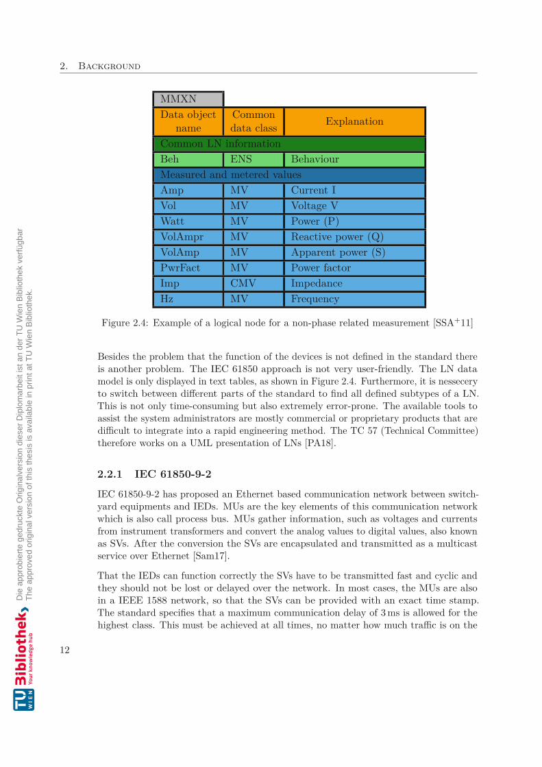
Modelling This topic deals with the mapping of physical system data into a formaldata model which is defined by the standard. Logical Nodes (LNs) are used tomodel devices and functions of the power system. Among other things, they can beused to model power system components such as switches, transformers or invertersas well as power system functions such as measurement, protection or voltagecontrol which can also be seen in Figure 2.3. Therefore, they are among the mostimportant part of modelling [PA18]. Figure 2.4 shows an example of a LN for anon-phase related measurement (MMXN). It can be seen that the properties ofLNs are presented in a tabular format [SSA+11].

Configuration The second main topic of IEC 61850 is the configuration of the othertwo main topics. Part 6 - “Configuration description language for communicationin electrical substations related to IEDs” - of the standard describes the SystemConfiguration description Language (SCL) based on Extensible Markup Language(XML). With this configuration tool it is possible to configure a complete powerutility system [SSA+11]. The SCL can be used to describe which components andfunctions are modelled, from a whole substation to a single IED. Furthermore, it

10

2.2. IEC 61850 - Communication networks and systems for power utility automation

EthernetNetwork

2 Configuration

1 Model

TapCtrl

DER

LN LN

LN LNLN

XCBR

Pos

OpCnt

3 Communication

Abs

trac

tC

omm

unic

atio

nSe

rvic

esM

appi

ngM

MS

TC

P/IP

Virtualization

TapCtrl

DER

Figure 2.3: Overview of IEC 61850 three main topics: 1 Modelling, 2 Configuration,3 Communication [PA18]

can also be configured which service and which protocol should be used to exchangeinformation. Finally, SCL also provides tools for modeling and configuring parts ofthe communication network. The result is a configuration file that can be used toconfigure the different devices in the system [PA18].

Communication The last main topic defines the different communication services thatare available to transfer data between IEDs. For example, client-server-basedcommunication is defined where the information is polled or reported, as wellas publisher-subscriber-based communication or real-time communication usingGeneric Object Oriented Substation Event (GOOSE). GOOSE offer a fast andreliable transmission of critical substation events between control and protectiondevices which improves system stability and performance [HHFK17]. The standardalso defines different mappings between communication services and different proto-cols. An example of such a mapping is the mapping of a client-server communicationto the Manufacturing Message Specification (MMS) which is defined in Part 8-1- “Specific communication service mapping (SCSM) - Mappings to MMS (ISO9506-1 and ISO 9506-2) and to ISO/IEC 8802-3” [TC 19].

11

2. Background

MMXNData object

nameCommondata class Explanation

Common LN informationBeh ENS BehaviourMeasured and metered valuesAmp MV Current IVol MV Voltage VWatt MV Power (P)VolAmpr MV Reactive power (Q)VolAmp MV Apparent power (S)PwrFact MV Power factorImp CMV ImpedanceHz MV Frequency

Figure 2.4: Example of a logical node for a non-phase related measurement [SSA+11]

Besides the problem that the function of the devices is not defined in the standard thereis another problem. The IEC 61850 approach is not very user-friendly. The LN datamodel is only displayed in text tables, as shown in Figure 2.4. Furthermore, it is nesseceryto switch between different parts of the standard to find all defined subtypes of a LN.This is not only time-consuming but also extremely error-prone. The available tools toassist the system administrators are mostly commercial or proprietary products that aredifficult to integrate into a rapid engineering method. The TC 57 (Technical Committee)therefore works on a UML presentation of LNs [PA18].

2.2.1 IEC 61850-9-2

IEC 61850-9-2 has proposed an Ethernet based communication network between switch-yard equipments and IEDs. MUs are the key elements of this communication networkwhich is also call process bus. MUs gather information, such as voltages and currentsfrom instrument transformers and convert the analog values to digital values, also knownas SVs. After the conversion the SVs are encapsulated and transmitted as a multicastservice over Ethernet [Sam17].

That the IEDs can function correctly the SVs have to be transmitted fast and cyclic andthey should not be lost or delayed over the network. In most cases, the MUs are alsoin a IEEE 1588 network, so that the SVs can be provided with an exact time stamp.The standard specifies that a maximum communication delay of 3 ms is allowed for thehighest class. This must be achieved at all times, no matter how much traffic is on the

12

2.3. IEEE 1588

process bus communication network. GOOSE and SV packages belong to the highestclass and thus to the most time-critical messages. These messages are mapped directlyto the Data Layer and not to the Transport Layer of the OSI Model. As a result, thetime-critical messages are transmitted without transmission reliability. This means thatno acknowledgment will be sent if the packet has been received or the packet is notretransmitted if it is lost during transmission. Therefore, it has been defined in theStandard IEC 61850-8-1 that GOOSE messages should be transmitted several times inorder to improve transmission reliability. This approach can not be used for SVs as theyare continuously fed into the network by multiple MUs at a rate of 80 Samples Per Cycle(SPC). By sending the same package multiple times, the network load would be increasedenormously. It was therefore decided that there are no assurance or reliability measuresfor SV communication over the process bus [KSZ11].

On the other hand, the IEC 61850-9 process bus also offers advantages. First, it’s interop-erability. With this process bus, all connected devices can exchange any information withthe IEDs or MUs, even if they are from different manufacturers. Furthermore, the entirecommunication network is simplified, as many point-to-point connections are replaced bya few Ethernet connections. This makes the entire communication network much clearerand easier to maintain. And last but not least, both the installation costs and the laborcosts can be significantly reduced because, as already mentioned, the entire network canbe simplified [KSZ11].

2.2.2 IEC 61850-9-2-LEIEC 61850-9-2-LE (Light Edition) is just an implementation guideline and is basedon the IEC 61850 standard. This document is used by most vendors manufacturingIEC 61850-9-2 compatible devices. The guideline was published by the UCA InternationalUsers Group. Among other things, this guideline defines that a SV stream transmits 8instantaneous values. The three phases and neutral values for current and voltage. Thesevalues are measured at a fixed sampling rate of 80 or 256 SPC. This means that 4000 or12 800 frames per second are transmitted at a network frequency of 50 Hz [KRP18].

In Figure B.1 shows the content of an Ethernet frame, which is used to transmit SVs.Furthermore, in Figure B.2 the Application Protocol Data Unit (APDU) data field isshown in more detail. As demonstrated the APDU data field is divided into many values.The sample counter (smpCnt) is one of those values. This value allows the receivers tomatch the samples of different MUs in the correct order. This value is set to zero aftereach period and then incremented by one with each sample [HS07].

2.3 IEEE 1588In a SAS all devices must have the same time reference, so that the global time behaviourcan be analyzed and in case of a fault, it can be precisely analyzed why, when and wherethe error occurred. For samples of currents and voltages a time synchronization accuracy

13

2. Background

in the order of 1 µs is needed. For the fault detection and location on the transmissionlines of the power grid a synchronization accuracy of less than 1 µs is needed because atime error of 1 µs results in a location error of 300 m [BLW03, MML+16].

Inter Range Instrumentation Group-B (IRIG-B) was originally used as a synchronizationscheme in substations. This allowed an accuracy of 1 µs to be achieved. To achievethis accuracy, an extra cabling infrastructure had to be created, which in most caseswas not redundant and therefore very prone to error. As a result, the implementationand maintenance costs were extremely high. Another problem was that the variousdevices were located at different distances from the control building, resulting in differentpropagation delays that could only be compensated with the help of complicated andbothersome calibration processes [DFF+11].

Today, the trend is toward using a single Ethernet-based data network for all kind ofcommunication. With the Simple Network Time Protocol (SNTP) an accuracy of 1 mscan be achieved, which is needed to perform a post-event fault analysis. However, mostexperts recommend for high precision time synchronization in SASs to use the PTP,which is defined in the IEEE 1588 standard [MML+16].

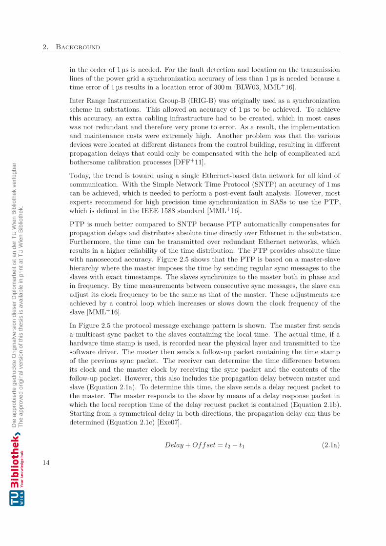
PTP is much better compared to SNTP because PTP automatically compensates forpropagation delays and distributes absolute time directly over Ethernet in the substation.Furthermore, the time can be transmitted over redundant Ethernet networks, whichresults in a higher reliability of the time distribution. The PTP provides absolute timewith nanosecond accuracy. Figure 2.5 shows that the PTP is based on a master-slavehierarchy where the master imposes the time by sending regular sync messages to theslaves with exact timestamps. The slaves synchronize to the master both in phase andin frequency. By time measurements between consecutive sync messages, the slave canadjust its clock frequency to be the same as that of the master. These adjustments areachieved by a control loop which increases or slows down the clock frequency of theslave [MML+16].

In Figure 2.5 the protocol message exchange pattern is shown. The master first sendsa multicast sync packet to the slaves containing the local time. The actual time, if ahardware time stamp is used, is recorded near the physical layer and transmitted to thesoftware driver. The master then sends a follow-up packet containing the time stampof the previous sync packet. The receiver can determine the time difference betweenits clock and the master clock by receiving the sync packet and the contents of thefollow-up packet. However, this also includes the propagation delay between master andslave (Equation 2.1a). To determine this time, the slave sends a delay request packet tothe master. The master responds to the slave by means of a delay response packet inwhich the local reception time of the delay request packet is contained (Equation 2.1b).Starting from a symmetrical delay in both directions, the propagation delay can thus bedetermined (Equation 2.1c) [Exe07].

Delay + Offset = t2 − t1 (2.1a)

14

2.4. EtherCAT

MasterClock

SlaveClock

t1

t2

Sync

Follow_Up(t1)

t3

t4

Delay_Re

q

Delay_Resp(t4)

Offset

Master toSlave delay

OffsetMaster toSlave delay

Figure 2.5: IEEE 1588 protocol message exchange pattern [MML+16].

Delay − Offset = t4 − t3 (2.1b)

Delay = (t2 − t1) + (t4 − t3)2 (2.1c)

The measurement of the propagation delay takes place in intervals of 1 s to 64 s. Thesynchronization process by sending the sync packets is done every 2 s to 8 s, because thedrift rate of the local clocks generally causes a greater impact per time interval thanthe slow changing propagation delay. The accuracy of clock synchronization achieveddepends primarily on whether PTP is implemented using hardware time stamping ornot [MES14].

2.4 EtherCATEtherCAT was developed by Beckhoff1 and is part of the IEC standard since 2005. Thetechnology is supported and fostered by users who have joined the EtherCAT Technology

1https://www.beckhoff.de/

15

2. Background

Group (ETG) [Dü17].

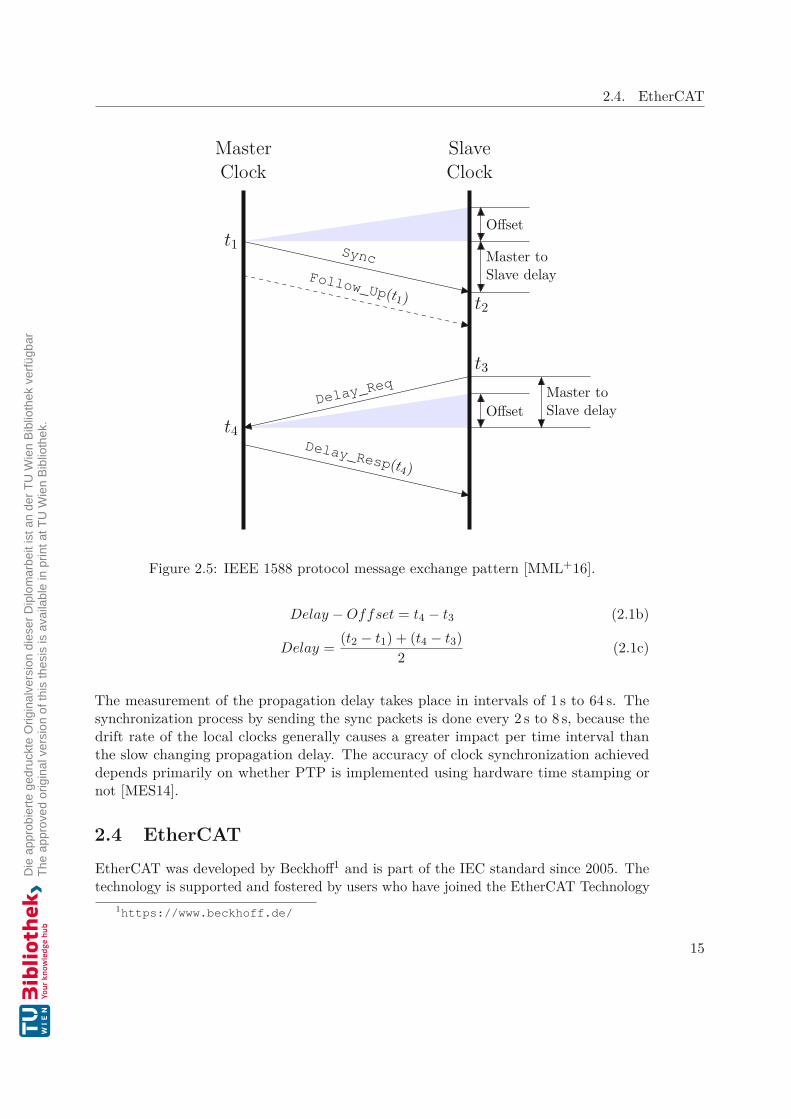
A EtherCAT system consists of a single master and several slaves logically connectedby a ring topology, as shown in Figure 2.6. The subscribers of a EtherCAT network arephysically arranged in a line if there is no branch. However, as illustrated in Figure 2.6,it is also possible to build a physical tree topology by branching in the return channel.The telegram first runs from a branch along a path to the last participant of this pathand is sent back by this to the branch. There the telegram is then directed to the otherpath. Logically speaking, it is still a ring topology [WB05].

Master

Figure 2.6: EtherCAT topology with branches [WB05]

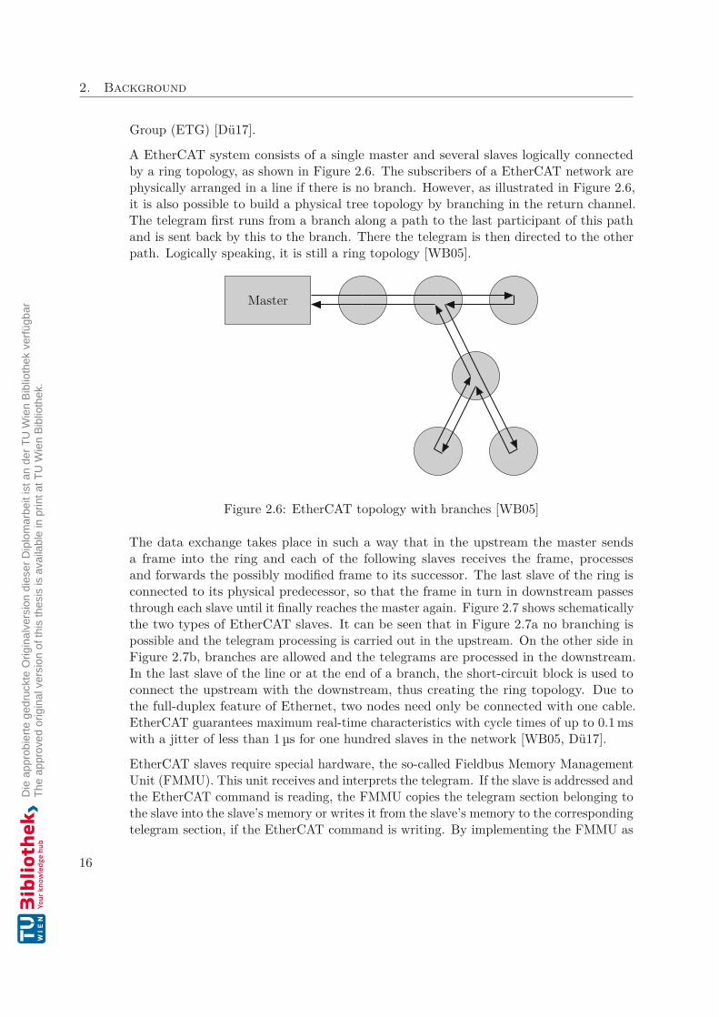
The data exchange takes place in such a way that in the upstream the master sendsa frame into the ring and each of the following slaves receives the frame, processesand forwards the possibly modified frame to its successor. The last slave of the ring isconnected to its physical predecessor, so that the frame in turn in downstream passesthrough each slave until it finally reaches the master again. Figure 2.7 shows schematicallythe two types of EtherCAT slaves. It can be seen that in Figure 2.7a no branching ispossible and the telegram processing is carried out in the upstream. On the other side inFigure 2.7b, branches are allowed and the telegrams are processed in the downstream.In the last slave of the line or at the end of a branch, the short-circuit block is used toconnect the upstream with the downstream, thus creating the ring topology. Due tothe full-duplex feature of Ethernet, two nodes need only be connected with one cable.EtherCAT guarantees maximum real-time characteristics with cycle times of up to 0.1 mswith a jitter of less than 1 µs for one hundred slaves in the network [WB05, Dü17].

EtherCAT slaves require special hardware, the so-called Fieldbus Memory ManagementUnit (FMMU). This unit receives and interprets the telegram. If the slave is addressed andthe EtherCAT command is reading, the FMMU copies the telegram section belonging tothe slave into the slave’s memory or writes it from the slave’s memory to the correspondingtelegram section, if the EtherCAT command is writing. By implementing the FMMU as

16

2.4. EtherCAT

Rx Telegramprocessing Tx

shortcircuit

Tx Rx

up-stream

down-stream

Branch

(a) without branches

Rx Tx

Tx Rx

Telegramprocessing

shortcircuitRx Tx

Branch

up-stream

down-stream

(b) with branches

Figure 2.7: Two different EtherCAT slave types [WB05]

an Application-Specific Integrated Circuit (ASIC), the time for these operations is in therange of nanosecond [WB05].

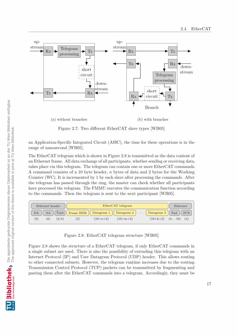
The EtherCAT telegram which is shown in Figure 2.8 is transmitted as the data content ofan Ethernet frame. All data exchange of all participants, whether sending or receiving data,takes place via this telegram. The telegram can contain one or more EtherCAT commands.A command consists of a 10 byte header, n bytes of data and 2 bytes for the WorkingCounter (WC). It is incremented by 1 by each slave after processing the commands. Afterthe telegram has passed through the ring, the master can check whether all participantshave processed the telegram. The FMMU executes the communication function accordingto the commands. Then the telegram is sent to the next participant [WB05].

Type

(2/4)(6)

SA

(6)

DA

Ethernet header

(2)

Frame HDR

ECAT

(10+n+2)

Datagram 1

(10+m+2)

Datagram 2 . . .

(10+k+2)

Datagram 3

EtherCAT telegram

(0. . . 32)

Pad.

(4)

FCS

Ethernet

Figure 2.8: EtherCAT telegram structure [WB05]

Figure 2.8 shows the structure of a EtherCAT telegram, if only EtherCAT commands ina single subnet are used. There is also the possibility of extending this telegram with anInternet Protocol (IP) and User Datagram Protocol (UDP) header. This allows routingto other connected subnets. However, the telegram runtime increases due to the routing.Transmission Control Protocol (TCP) packets can be transmitted by fragmenting andpasting them after the EtherCAT commands into a telegram. Accordingly, they must be

17

2. Background

reassembled at the receiver by the EtherCAT software [Dü17].

2.5 Measuring device - TESTRANO 600This chapter explains the measuring device, which was used for this thesis and showsa possible experimental setup for the purpose of this diploma thesis. Furthermore, thesoftware architecture of the embedded system is described and how this thesis can beintegrated in the already running system without disturbing it.

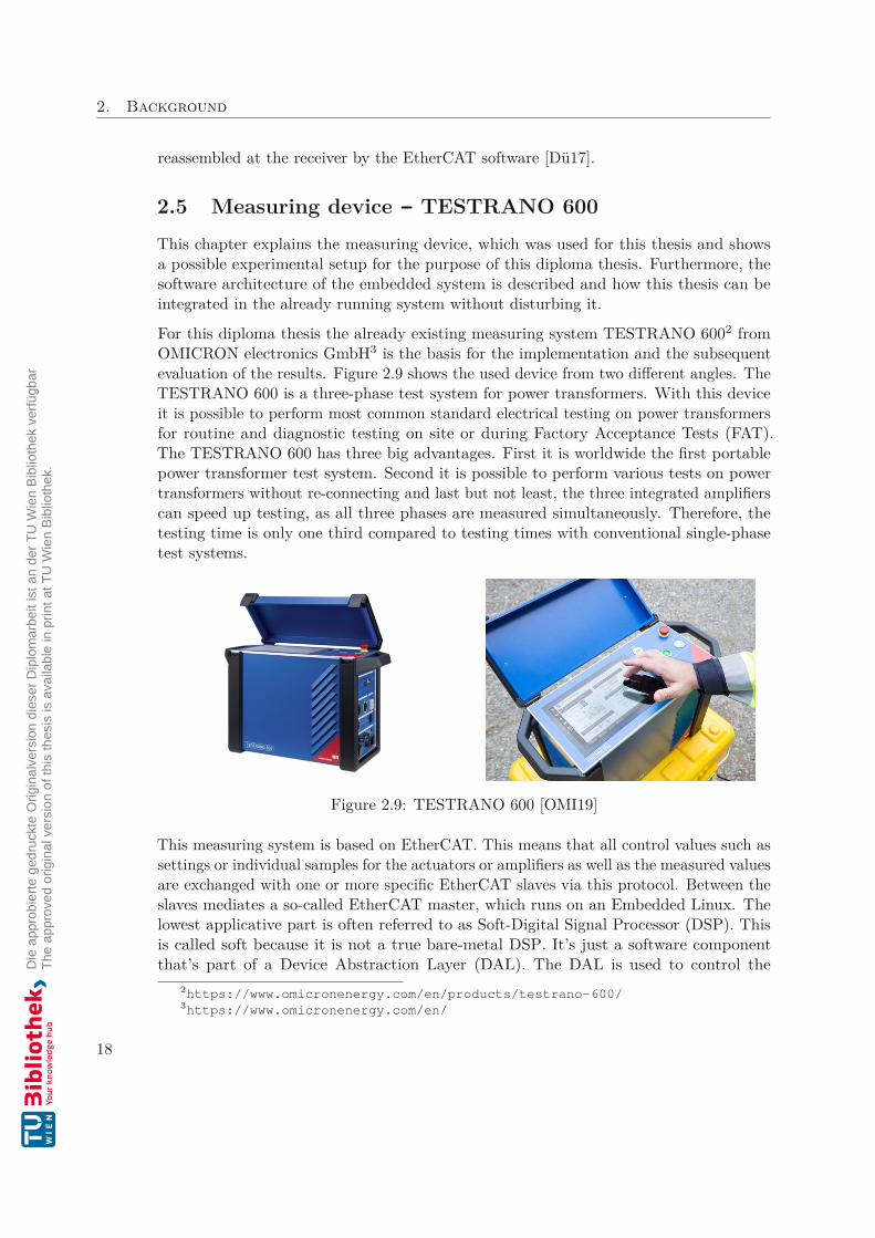
For this diploma thesis the already existing measuring system TESTRANO 6002 fromOMICRON electronics GmbH3 is the basis for the implementation and the subsequentevaluation of the results. Figure 2.9 shows the used device from two different angles. TheTESTRANO 600 is a three-phase test system for power transformers. With this deviceit is possible to perform most common standard electrical testing on power transformersfor routine and diagnostic testing on site or during Factory Acceptance Tests (FAT).The TESTRANO 600 has three big advantages. First it is worldwide the first portablepower transformer test system. Second it is possible to perform various tests on powertransformers without re-connecting and last but not least, the three integrated amplifierscan speed up testing, as all three phases are measured simultaneously. Therefore, thetesting time is only one third compared to testing times with conventional single-phasetest systems.

Figure 2.9: TESTRANO 600 [OMI19]

This measuring system is based on EtherCAT. This means that all control values such assettings or individual samples for the actuators or amplifiers as well as the measured valuesare exchanged with one or more specific EtherCAT slaves via this protocol. Between theslaves mediates a so-called EtherCAT master, which runs on an Embedded Linux. Thelowest applicative part is often referred to as Soft-Digital Signal Processor (DSP). Thisis called soft because it is not a true bare-metal DSP. It’s just a software componentthat’s part of a Device Abstraction Layer (DAL). The DAL is used to control the

2https://www.omicronenergy.com/en/products/testrano-600/3https://www.omicronenergy.com/en/

18

2.5. Measuring device - TESTRANO 600

EtherCAT master running on the same Linux system. The Soft-DSP enables largelyfreely configurable signal routing between the individual data fields of the EtherCATframes and performs simple calculations that can be performed on an embedded processorwith limited Floating-Point Unit (FPU) or for embedded systems typically medium-speedArithmetic Logic Unit (ALU).

The amplifier and measuring technology are represented and made accessible by theEtherCAT slaves. During a measurement these slaves communicate with the embeddedsystem with 10 kHz hard real-time. These slaves are usually associated with an assetin order to stimulate them and measure the results mainly from these stimuli. Besidesvoltages and currents sometimes movements and very often time response are measured.For this diploma thesis the most relevant assets are the instrument transformers (CTsand VTs).

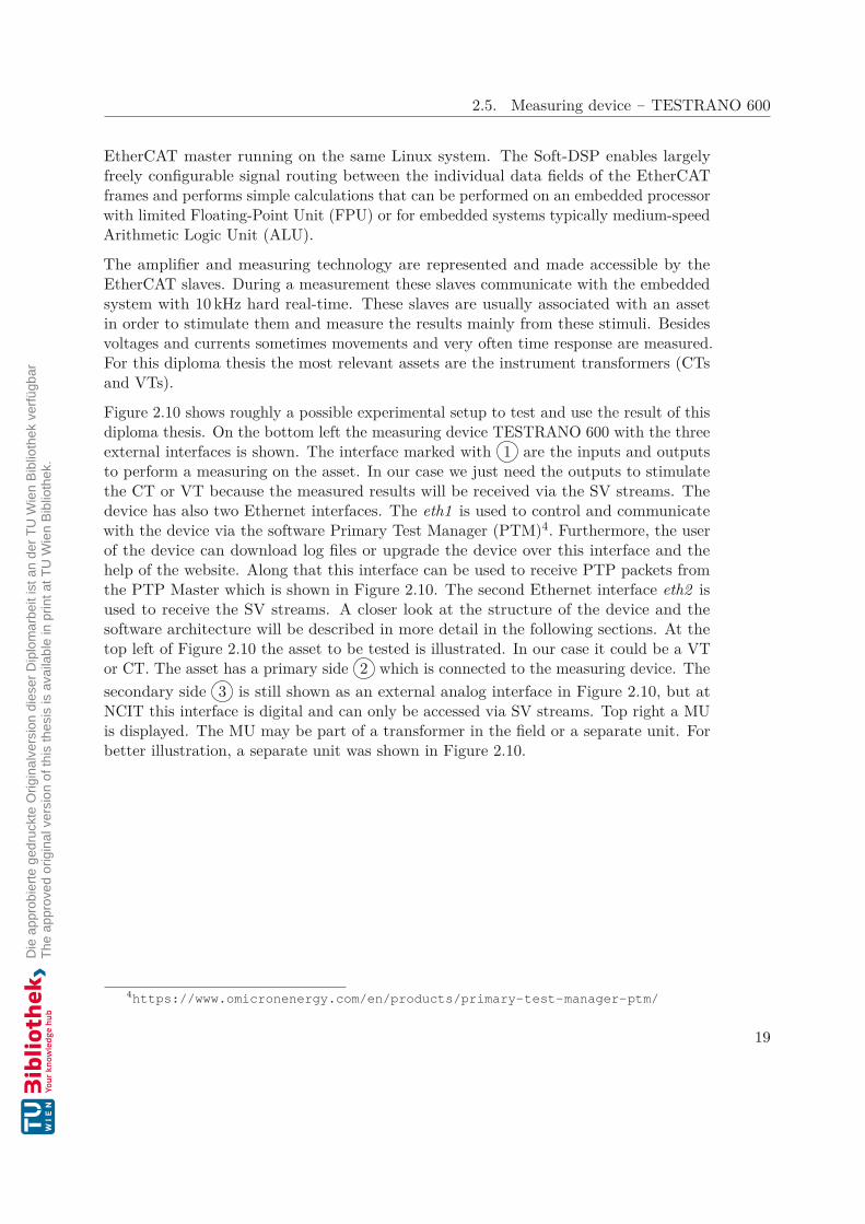
Figure 2.10 shows roughly a possible experimental setup to test and use the result of thisdiploma thesis. On the bottom left the measuring device TESTRANO 600 with the threeexternal interfaces is shown. The interface marked with 1 are the inputs and outputsto perform a measuring on the asset. In our case we just need the outputs to stimulatethe CT or VT because the measured results will be received via the SV streams. Thedevice has also two Ethernet interfaces. The eth1 is used to control and communicatewith the device via the software Primary Test Manager (PTM)4. Furthermore, the userof the device can download log files or upgrade the device over this interface and thehelp of the website. Along that this interface can be used to receive PTP packets fromthe PTP Master which is shown in Figure 2.10. The second Ethernet interface eth2 isused to receive the SV streams. A closer look at the structure of the device and thesoftware architecture will be described in more detail in the following sections. At thetop left of Figure 2.10 the asset to be tested is illustrated. In our case it could be a VTor CT. The asset has a primary side 2 which is connected to the measuring device. Thesecondary side 3 is still shown as an external analog interface in Figure 2.10, but atNCIT this interface is digital and can only be accessed via SV streams. Top right a MUis displayed. The MU may be part of a transformer in the field or a separate unit. Forbetter illustration, a separate unit was shown in Figure 2.10.

4https://www.omicronenergy.com/en/products/primary-test-manager-ptm/

19

2. Background

Testrano 600eth1

eth21

CTVT2 3 MU4

ptp

eth1

PTPMaster

ptp

PCeth1

1 Analogue measuring signal outputs 2 CT/VT primary side

3 CT/VT secondary side 4 Analogue measuring signal inputs

Figure 2.10: Possible experimental setup for this diploma thesis

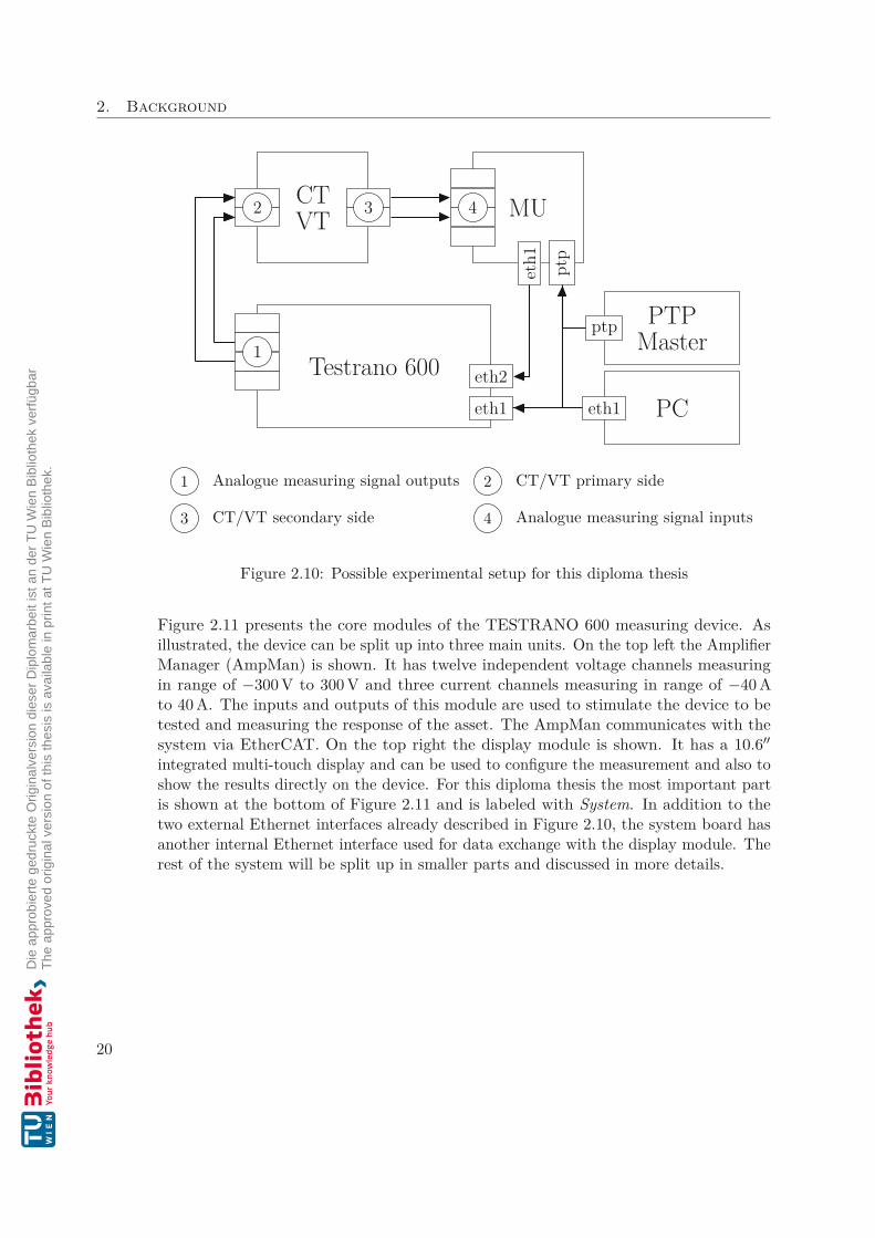
Figure 2.11 presents the core modules of the TESTRANO 600 measuring device. Asillustrated, the device can be split up into three main units. On the top left the AmplifierManager (AmpMan) is shown. It has twelve independent voltage channels measuringin range of −300 V to 300 V and three current channels measuring in range of −40 Ato 40 A. The inputs and outputs of this module are used to stimulate the device to betested and measuring the response of the asset. The AmpMan communicates with thesystem via EtherCAT. On the top right the display module is shown. It has a 10.6integrated multi-touch display and can be used to configure the measurement and also toshow the results directly on the device. For this diploma thesis the most important partis shown at the bottom of Figure 2.11 and is labeled with System. In addition to thetwo external Ethernet interfaces already described in Figure 2.10, the system board hasanother internal Ethernet interface used for data exchange with the display module. Therest of the system will be split up in smaller parts and discussed in more details.

20

2.5. Measuring device - TESTRANO 600

AmpMan Display

System

1

Ethe

r-C

AT eth0

Ethe

r-C

AT eth0

eth2

eth1

1 Analogue measuring signal outputs

Figure 2.11: Core modules of the TESTRANO 600

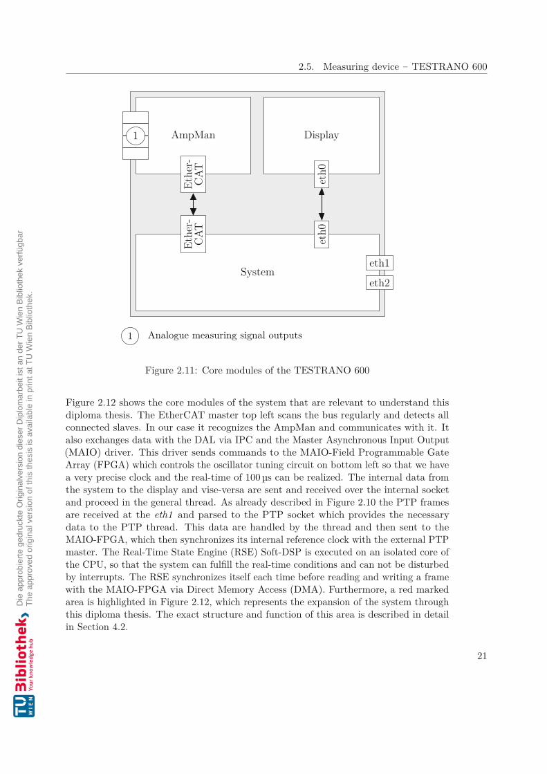
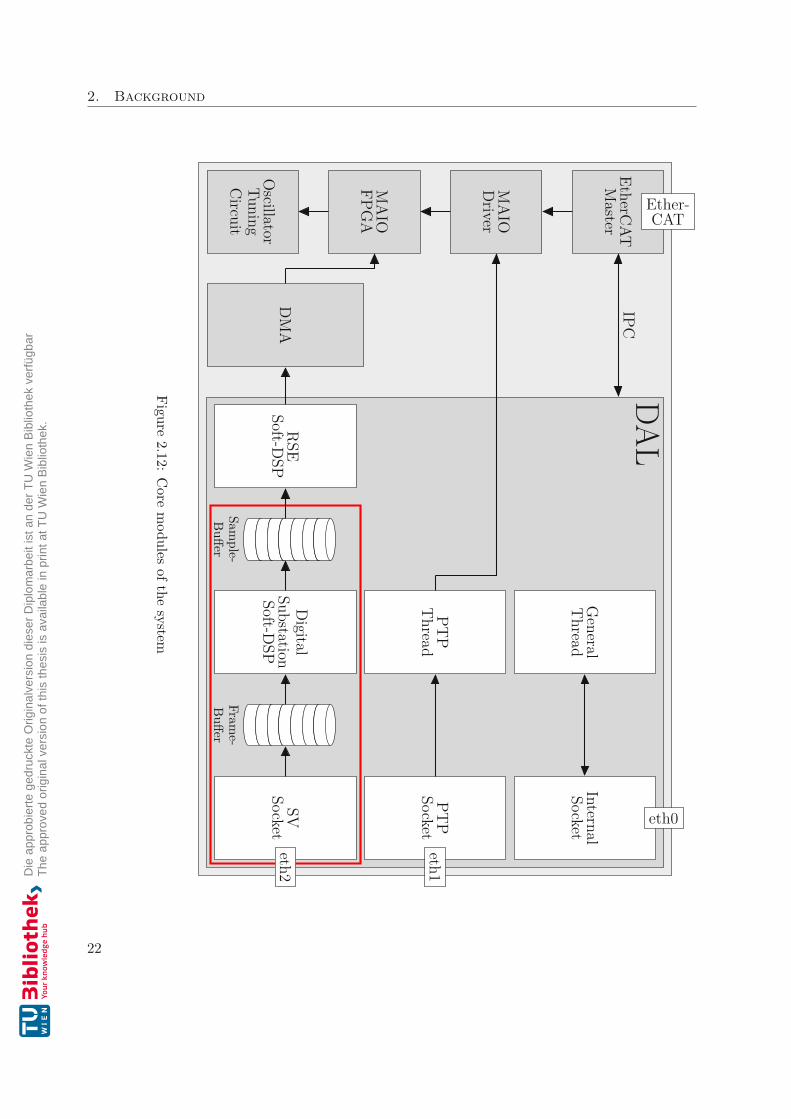
Figure 2.12 shows the core modules of the system that are relevant to understand thisdiploma thesis. The EtherCAT master top left scans the bus regularly and detects allconnected slaves. In our case it recognizes the AmpMan and communicates with it. Italso exchanges data with the DAL via IPC and the Master Asynchronous Input Output(MAIO) driver. This driver sends commands to the MAIO-Field Programmable GateArray (FPGA) which controls the oscillator tuning circuit on bottom left so that we havea very precise clock and the real-time of 100 µs can be realized. The internal data fromthe system to the display and vise-versa are sent and received over the internal socketand proceed in the general thread. As already described in Figure 2.10 the PTP framesare received at the eth1 and parsed to the PTP socket which provides the necessarydata to the PTP thread. This data are handled by the thread and then sent to theMAIO-FPGA, which then synchronizes its internal reference clock with the external PTPmaster. The Real-Time State Engine (RSE) Soft-DSP is executed on an isolated core ofthe CPU, so that the system can fulfill the real-time conditions and can not be disturbedby interrupts. The RSE synchronizes itself each time before reading and writing a framewith the MAIO-FPGA via Direct Memory Access (DMA). Furthermore, a red markedarea is highlighted in Figure 2.12, which represents the expansion of the system throughthis diploma thesis. The exact structure and function of this area is described in detailin Section 4.2.

21

2. Background

DALIPC

EtherCAT

Master

MA

IOD

river

MA

IOFPG

A

OscillatorTuningC

ircuit

DM

AR

SESoft-D

SP

Sample-

Buffer

Digital

SubstationSoft-D

SP

Frame-

Buffer

SVSocket

PTP

SocketPT

PT

hread

InternalSocket

General

Thread

Ether-CAT

eth0

eth1

eth2

Figure2.12:

Core

modules

ofthesystem

22

CHAPTER 3Related Work

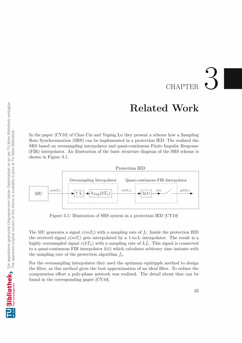
In the paper [CY10] of Chao Cai and Yuping Lu they present a scheme how a SamplingRate Synchronization (SRS) can be implemented in a protection IED. The realized theSRS based on oversampling interpolator and quasi-continuous Finite Impulse Response(FIR) interpolator. An illustration of the basic structure diagram of the SRS scheme isshown in Figure 3.1.

↑ L hDig(kTn)

Oversampling Interpolator

h(t)v(kTn) y(t)

Quasi-continuous FIR Interpolator

y(kTo)

Protection IED

MUx(mTi)

Figure 3.1: Illustration of SRS system in a protection IED [CY10]

The MU generates a signal x(mTi) with a sampling rate of fi. Inside the protection IEDthe received signal x(mTi) gets interpolated by a 1-to-L interpolator. The result is ahighly oversampled signal v(kTn) with a sampling rate of Lfi. This signal is connectedto a quasi-continuous FIR interpolator h(t) which calculates arbitrary time instants withthe sampling rate of the protection algorithm fo.

For the oversampling interpolator they used the optimum equiripple method to designthe filter, as this method gives the best approximation of an ideal filter. To reduce thecomputation effort a poly-phase network was realized. The detail about that can befound in the corresponding paper [CY10].

23

3. Related Work

For the quasi-continuous FIR interpolator the number of calculations and therefore theorder of the filter should be as low as possible but with decreasing the order of thefilter the difficulty to design such a filter increases. Therefore, it is important to find acompromise where the amount of calculations as well as the complexity of the design isconsidered.

For the evaluation they compared the proposed SRS scheme with a zero-order-holderfollowed by the oversampling interpolator and the cubic spline interpolation. For thetest setup with an oversampling factor L = 20 the presented SRS scheme has aninstantaneous current error within 0.5%. With the zero-order-holder following theoversampling interpolator with the same oversampling factor L the instantaneous currenterror is larger than the previous one. Some experiments showed that an oversamplingfactor L ≥ 40 is needed to get an error within 0.5%. The instantaneous current error of thecubic spline interpolation is comparable to the one of the proposed SRS scheme. The exactresults and the diagrams of the measurement can be found in the paper [CY10]. Withthe cubic spline interpolation the needed SRS could also be achieved but in this paperthe authors wanted to use the full high speed computing capacity of the DSP [CY10].

For our thesis the SRS will be done in a Soft-DSP and therefore we can not use thisspecial computing capacity of a DSP. Because of that, this proposed SRS scheme of ChaoCai and Yuping Lu is not really suitable for our problem.

R. Tao, B. Jiang and C. Wang described in their paper [TJW11] the problem thatin a SAS often Electronic Instrument Transformerss (EITs) are provided from differentmanufacturers and therefore it can happen that they use different sampling rates becauseof different standards of the manufacturers. Due to a probable mismatch between theEITs and the IED the data cannot directly be transmitted. In this paper [TJW11] theyshowed how this problem can be solved in a full digitalization process using interpolationand decimation methods.

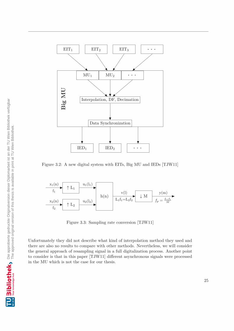
Therefore, they presented the Big MU which does the sampling rate conversion andafterwards a data synchronization. An illustration of this Big MU can be found inFigure 3.2. The MUs receive data from the EITs and send them to the next module whichincludes an interpolation method, a Digital Filter (DF) and a decimation algorithm. Theresulting asynchronous data are then forwarded to the data synchronization module toget synchronized data again which then can be transmitted to the IEDs.

Figure 3.3 shows the steps needed to convert a sampling rate. The signals x1(n) andx2(n) are two data channels from MU1 and MU2 with the sampling frequencies f1 andf2 where f1 = f2. The two data channels get interpolated by factor L1 and L2 and thenlow-pass filtered by h(n). After that the data get decimated by a factor of M and theresult is the data sequence y(m) with the sampling frequency of fp = L1·f1

M

For the data synchronization they used the quadratic interpolation method. The simula-tion of the Big MU showed good results and can be found in the paper [TJW11]. Forthis thesis we could see the general idea of resampling data and how this could be done.

24

MU1 MU2 . . .

EIT2EIT1 EIT3 . . .

Interpolation, DF, Decimation

Data Synchronization

Big

MU

IED2IED1 . . .

Figure 3.2: A new digital system with EITs, Big MU and IEDs [TJW11]

↑ L1

↑ L2

h(n) ↓ M

x1(n)f1

x2(n)f2

u1(l1)

u2(l2)

v(l)L1f1=L2f2

y(m)

fp = L1f1M

Figure 3.3: Sampling rate conversion [TJW11]

Unfortunately they did not describe what kind of interpolation method they used andthere are also no results to compare with other methods. Nevertheless, we will considerthe general approach of resampling signal in a full digitalization process. Another pointto consider is that in this paper [TJW11] different asynchronous signals were processedin the MU which is not the case for our thesis.

25

3. Related Work

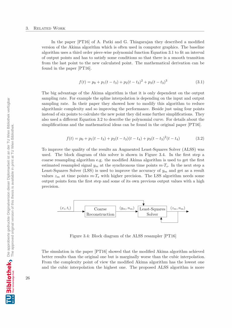
In the paper [PT16] of A. Patki and G. Thiagarajan they described a modifiedversion of the Akima algorithm which is often used in computer graphics. The baselinealgorithm uses a third order piece-wise polynomial function Equation 3.1 to fit an intervalof output points and has to satisfy some conditions so that there is a smooth transitionfrom the last point to the new calculated point. The mathematical derivation can befound in the paper [PT16].

f(t) = p0 + p1(t − t3) + p2(t − t3)2 + p3(t − t3)3 (3.1)

The big advantage of the Akima algorithm is that it is only dependent on the outputsampling rate. For example the spline interpolation is depending on the input and outputsampling rate. In their paper they showed how to modify this algorithm to reducealgorithmic complexity and so improving the performance. Beside just using four pointsinstead of six points to calculate the new point they did some further simplifications. Theyalso used a different Equation 3.2 to describe the polynomial curve. For details about thesimplifications and the mathematical ideas can be found in the original paper [PT16].

f(t) = p0 + p1(t − t3) + p2(t − t3)(t − t4) + p3(t − t3)2(t − t4) (3.2)

To improve the quality of the results an Augmented Least-Squares Solver (ALSS) wasused. The block diagram of this solver is shown in Figure 3.4. In the first step acoarse resampling algorithm e.g. the modified Akima algorithm is used to get the firstestimated resampled signal ym at the synchronous time points m·Ts. In the next step aLeast-Squares Solver (LSS) is used to improve the accuracy of ym and get as a resultvalues zm at time points m·Ts with higher precision. The LSS algorithm needs someoutput points form the first step and some of its own previous output values with a highprecision.

CoarseReconstruction

Least-SquaresSolver

(xi, ti) (ym, nm) (zm, nm)

Figure 3.4: Block diagram of the ALSS resampler [PT16]

The simulation in the paper [PT16] showed that the modified Akima algorithm achievedbetter results than the original one but is marginally worse than the cubic interpolation.From the complexity point of view the modified Akima algorithm has the lowest oneand the cubic interpolation the highest one. The proposed ALSS algorithm is more

26

complex than the modified Akima algorithm and has a similar performance than thecubic interpolation algorithm. So the conclusion is that the modified Akima scheme issuitable for low complexity and medium performance applications and the ALSS schemeshould be used for medium complexity and high performance applications.

For our thesis we would need to go for the ALSS algorithm but we can not really benefitbecause this algorithm is optimized for asynchronous to synchronous resampling andwe just need a resampling algorithm and therefore the cubic interpolation can also besimplified as we know that we have already synchronous samples at the input. So theresults are anyways almost the same and the complexity of the cubic interpolation canbe reduced with the information that we have equidistant sample points.

Yeying Chen, Enrico Mohns, Michael Seckelmann and Soeren de Rose described intheir paper a precise amplitude and phase determination for calibrating SV instrumentsby using resampling algorithms [CMSdR20]. For the resampling process they used amodified sinc interpolation in the time domain. Furthermore, a phase correction isdescribed to preserve the phase accuracy to the 1 PPS signal.

Calculation ofresamplingparameters

ResamplingFrequencydetermination

Generator(sampling values)

U1f1ϕ1

NoiseHarmonics

NTs

FFT spectrum analysisu[k] u'[i]

Amplitude

Error

Phase

Error

u[k] u[k]f1'

u[k]TW 'N 'TS '

Figure 3.5: Program structure of the resampling process [CMSdR20]

Figure 3.5 shows the program structure of the used resampling process. The discretesignal samples u[k] covers three components which are a fundamental sinusoidal signal, awhite noise signal and a series of sinusoidal signals to simulate several harmonics. Themathematical equation to generate this signal is shown in Equation 3.3 where TS is thesampling time of the process. U1 and Um are the Root Mean Square (RMS) voltagesof the fundamental sinusoidal signal and the mth harmonic signal. f1 and fm are thefrequencies of the signals and ϕ1 and ϕm are the phase angles. The white noise signal isgenerated with a white noise random generator with a rectangular distribution.

27

3. Related Work

u[k] =√

2·U1·sin(2π·f1·k·TS + ϕ1) + uNoise +m>1

√2·Um·sin(2π·fm·k·TS + ϕm) (3.3)

The Frequency determination block in Figure 3.5 uses the IEEE-STD-1057 four-parametersine wave fit algorithm to determine the fundamental frequency f1. In the next blockthe required parameters for the resampling process are calculated. The Resamplingblock contains of three different resampling algorithms to compare the results of thedifferent methods. It is possible to choose between a quadratic, cubic or the modifiedsinc interpolation. The result is a discrete signal u'[i] with a sampling rate of fS ' whichis higher than the original sampling rate.The Fast Fourier Transform (FFT) spectrum analysis evaluates the quality of the positiverelative amplitude errors |ΔU

U | and the positive phase errors |Δϕ|. The detail descriptionabout the modified sinc interpolation and the phase synchronization can be found in thepaper [CMSdR20].For the first simulation a pure sinusoidal signal was used without noise and the harmonicseries. The modified sinc interpolation had the lowest relative amplitude errors |ΔU

U |followed by the cubic interpolation and the quadratic interpolation. The phase errorsof the modified sinc and cubic interpolation was almost the same, only the quadraticinterpolation provided a bigger phase error. For the computation time the quadraticinterpolation was the fastest algorithm and needed about 8 ms at a sampling rate of20 kHz. The cubic interpolation was slightly slower and needed about 9 ms. By far theslowest algorithm was the modified sinc interpolation which needed about 250 ms. Thesimulation also showed that fluctuating parameters have no significant effect on theaccuracy of the resampling algorithms. Furthermore, the simulation pointed out thatwith increasing the sampling rate fs also the relative amplitude errors have a growingtrend for all resampling algorithms.As a next step the simulation was done with single harmonic interaction. The resultsshowed that the relative amplitude errors for the fundamental as well as for the harmonicsignal have almost the same errors for all algorithms. All of them showed an increasingtrend for a higher order of the harmonics. And the order of algorithms based on therelative amplitude errors is the same as for the fundamental signal. After that thesimulation was done with a harmonic series and the results were slightly higher thanthe resampling with a single harmonic. As a final step they simulate the modified sincinterpolation and checked the results when also white noise is involved. These resultsand all others can be found in more detail in the paper [CMSdR20].For this thesis this paper showed, that for low frequencies which is the case in a substationthe cubic interpolation has almost as good results as the proposed modified sinc interpo-lation. The main reason for not taking the modified sinc interpolation for this thesis isthe computation time which is much higher. In our case the resampling algorithm has torun on an embedded hard real-time system and therefore we have to take the compromisefor a slightly higher relative amplitude error but much lower computation time.

28

CHAPTER 4Implementation

4.1 Resample

As already mentioned in Section 1.1, our hard real-time measurement system runs at asystem frequency of 10 kHz, which can not be changed. It was also noted in Section 1.1that the SVs are received at 4000 Hz or 4800 Hz depending on the network frequency.Since the system frequency and the frequency of the SVs do not match, the SVs must beresampled so that the SVs are also available to the measuring system at a frequency of10 kHz.

Since 10 kHz is neither a multiple of 4000 Hz nor 4800 Hz, we first need to upsample to ahigher frequency than 10 kHz and then downsample again, so that we finally reach thedesired 10 kHz. Now the question arises, on which frequency we first have to upsample.The simplest solution is simply to multiply the two frequencies, but this does not alwaysgive the best solution, which means that unnecessary calculations are done and more timeis needed. The better approach is to calculate the least common frequency. A possibleimplementation is shown in Algorithm 4.1. By calling the function LCM with the twofrequencies the function will return the resulting upsampling frequency.

Algorithm 4.1: Calculation least common frequency1 function GCD(a, b): Greatest Common Divisor2 return ((b == 0) ? a : GCD(b, a mod b))3 end4 function LCM(a, b): Least Common Multiple5 return (a · b) / GCD(a, b)6 end

29

4. Implementation

In Subsection 4.1.1, the theoretical part of upsampling is first explained and a suitablealgorithm is selected. Subsequently, the selected algorithm is described in Subsection 4.1.3and in Subsection 4.1.4 the downsampling part is described.

4.1.1 UpsamplingThere are several options for upsampling. All algorithms have their advantages anddisadvantages, so we have to choose a variant that will give the best results for thespecific application. In the following points a few algorithms are presented and finallyan algorithm is selected. Of course there are further algorithms but they are not alldescribed in this diploma thesis.

Previous Neighbor Interpolation Previous Neighbor Interpolation is better knownas zero-order hold. With this method, the received SV is kept constant until thenext SV. It is a very simple method and does not require any calculations as theextra points between the two SVs will be the same as the last received SV. Thismethod is used in Analog-to-Digital Converters (ADCs). An illustration of themethod is shown in Figure 4.1.

Next Neighbor Interpolation This algorithm is very similar to the previously de-scribed algorithm. The only difference is, that this method does not keep the lastreceived SV constant, but the next received SV. This means that two SVs mustfirst be received before the interpolation can begin. Thus, the extra points betweenSV n and n + 1 all get the value of SV n + 1. Figure 4.2 shows an example of thealgorithm.

0 0.5 1 1.5 2 2.5 3 3.5 4 4.5 5 5.5 6−1

−0.8

−0.6

−0.4

−0.2

0

0.2

0.4

0.6

0.8

1

x

f(x)

Original ValuesUpsampled Values

Figure 4.1: Previous Neighbor

0 0.5 1 1.5 2 2.5 3 3.5 4 4.5 5 5.5 6−1

−0.8

−0.6

−0.4

−0.2

0

0.2

0.4

0.6

0.8

1

x

f(x)

Original ValuesUpsampled Values

Figure 4.2: Next Neighbor

Nearest Neighbor Interpolation This algorithm is a combination of the PreviousNeighbor and Next Neighbor Interpolation, as illustrated in Figure 4.3. With thismethod, not all additional points between the two SVs receive the same value.Any additional points before the time center of the two SVs will receive the value

30

4.1. Resample

according to the Previous Neighbor Interpolation and all values after the timecenter will get the value according to the Next Neighbor Interpolation. Even withthis method, no major calculations are needed. It only needs to be determined thetime, that is exactly in the middle of the two SVs.

Linear Interpolation Another simple method is the Linear Interpolation. The extrapoints between two SVs (xn, yn) and (xn+1, yn+1) can be easily calculated using thelinear relationship. Mathematically, the equation is established that the straight-linebetween the two SVs must have the same slope and ordinal distance as the straight-line between an additional point and a SV. After the mathematical transformation,Equation 4.1 is obtained, which can be used to calculate the additional points. Anexample of a Linear Interpolation is shown in Figure 4.4.

y = yn + (yn+1 − yn) · x − xn

xn+1 − xn(4.1)

0 0.5 1 1.5 2 2.5 3 3.5 4 4.5 5 5.5 6−1

−0.8

−0.6

−0.4

−0.2

0

0.2

0.4

0.6

0.8

1

x

f(x)

Original ValuesUpsampled Values

Figure 4.3: Nearest Neighbor

0 0.5 1 1.5 2 2.5 3 3.5 4 4.5 5 5.5 6−1

−0.8

−0.6

−0.4

−0.2

0

0.2

0.4

0.6

0.8

1

x

f(x)

Original ValuesUpsampled Values

Figure 4.4: Linear Interpolation

Polynomial Interpolation This method is a generalization of linear interpolation.Linear interpolation uses a linear function and this method replaces the interpolantwith a higher order polynomial. The order of the polynomial depends on thenumber of points used for the calculation. In general, we can say that for n points,there exists exactly one polynomial with the highest degree of n−1 passing throughall n points. So for the example shown in Figure 4.5 a polynomial of degree sixwas used, because all seven given points were used for the calculation.

Piecewise Cubic Spline Interpolation As described above, Linear Interpolation usesa linear function for each of the intervals [xn, xn+1]. For the Piecewise Cubic SplineInterpolation low order polynomials are used for each interval. The polynomialparts are selected so, that they fit together smoothly. Figure 4.6 shows an exampleof this interpolation method. Already anticipated, this algorithm provided the bestresults for this particular application and therefore this algorithm and mathematicalderivation is discussed and explained in more detail in Subsection 4.1.3.

31

4. Implementation

0 0.5 1 1.5 2 2.5 3 3.5 4 4.5 5 5.5 6−1.5

−1

−0.5

0

0.5

1

1.5

x

f(x)

Original ValuesUpsampled Values

Figure 4.5: Polynomial Interpolation

0 0.5 1 1.5 2 2.5 3 3.5 4 4.5 5 5.5 6−1

−0.8

−0.6

−0.4

−0.2

0

0.2

0.4

0.6

0.8

1

x

f(x)

Original ValuesUpsampled Values

Figure 4.6: Piecewise Cubic Spline

Shape-Preserving Piecewise Cubic Interpolation Like the cubic spline interpola-tion this method uses also the Piecewise Cubic Hermite Interpolating Polynomial(PCHIP). The only difference is, that the spline interpolation uses other conditionsfor the slopes at the given points. This algorithm tries to find a shape-preservinginterpolant that is visually pleasing. This is mainly achieved by determining theslopes at the given points, so that the function values do not overshoot the datavalues locally [Mol04]. An example of this method is shown in Figure 4.7.

0 0.5 1 1.5 2 2.5 3 3.5 4 4.5 5 5.5 6−1

−0.8

−0.6

−0.4

−0.2

0

0.2

0.4

0.6

0.8

1

x

f(x)

Original ValuesUpsampled Values

Figure 4.7: Shape-Preserving Piecewise Cubic

4.1.2 Selection of a suitable algorithmTo find a suitable algorithm for our problem we will compare the advantages anddisadvantages of the different methods and choose the algorithm based on this comparison.As a first step, we will start with the most simple algorithms. The big advantage ofthe Previous Neighbor, Next Neighbor and Nearest Neighbor Interpolation is that theextra points can be easily determined with less or none calculation. Furthermore, the

32

4.1. Resample

interpolation is really fast and does not use a lot of memory. If we have continuous signals,the results of these simple methods are unfortunately not perfect as clearly visible in theFigures 4.1 - 4.3. Depending on the sample rate of the received values the interpolationerror can get huge. That’s mainly the reason why these algorithms were not selected forthis diploma thesis.

The Linear Interpolation is also a very simple algorithm. The interpolated values can becalculated very easy and quick but on the other hand the interpolant is not differentiableat the received SV and therefore the result is not very smooth. Furthermore, the resultsare not very precise as shown in Figure 4.4.

The Polynomial Interpolation uses a polynomial of degree at most n − 1 passing throughall n SVs. Therefore, the interpolant is infinitely differentiable. It is therefore very easyto see that polynomial interpolation avoids the disadvantages of linear interpolation.Figure 4.5 shows, that the Polynomial Interpolation delivers a very good result with a verysmall interpolation error. Nevertheless, this method also has a significant disadvantage.The calculation of the interpolation polynomial is very computationally intensive andtakes a certain amount of time because some points are needed to get a good result.Therefore, this method was also not selected.

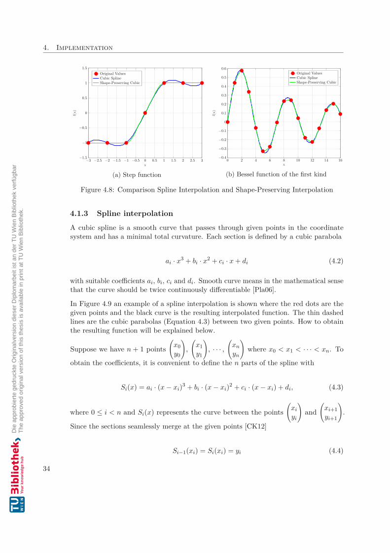
Finally, the two PCHIP methods are compared. The Shape-Preserving Piecewise CubicInterpolation is a local method and uses only two points to do the calculations. Thefirst derivative of the interpolant is continuous, but the second derivative is probablynot continuous. There may be jumps to the given points. On the other hand the SplineInterpolation is a global method which means, that the algorithm uses also points whichare more far away to do the calculations. The sensitivity to data far away is less thanto nearby data. Both algorithms have their advantages and disadvantages dependingon the signal to interpolate [Mol04]. An illustration of this dependency can be seen inFigure 4.8. On the left side in Figure 4.8a we have a step function. The illustrationshows clearly that the Cubic Interpolation has an oscillating result in the area of the step.The Shape-Preserving Piecewise Cubic Interpolation is much better suited for this typeof signal. On the other side in Figure 4.8b a Bessel function of the first kind is shown.This part of the image shows, that the Cubic Interpolation gives a better result in thearea of the peaks and is therefore better suited, if a continuous oscillating signal has tobe interpolated. From the complexity and the computational effort, the two methods areabout the same.

Since we only deal with sinus signals in our field of application, the Spline Interpolationwas chosen. In the next section the mathematical derivation will be explained and at theend the algorithm will be described.

33

4. Implementation

−3 −2.5 −2 −1.5 −1 −0.5 0 0.5 1 1.5 2 2.5 3−1.5

−1

−0.5

0

0.5

1

1.5

x

f(x)

Original ValuesCubic SplineShape-Preserving Cubic

(a) Step function

0 2 4 6 8 10 12 14 16−0.4

−0.3

−0.2

−0.1

0

0.1

0.2

0.3

0.4

0.5

0.6

x

f(x)

Original ValuesCubic SplineShape-Preserving Cubic

(b) Bessel function of the first kind

Figure 4.8: Comparison Spline Interpolation and Shape-Preserving Interpolation

4.1.3 Spline interpolationA cubic spline is a smooth curve that passes through given points in the coordinatesystem and has a minimal total curvature. Each section is defined by a cubic parabola

ai · x3 + bi · x2 + ci · x + di (4.2)

with suitable coefficients ai, bi, ci and di. Smooth curve means in the mathematical sensethat the curve should be twice continuously differentiable [Pla06].

In Figure 4.9 an example of a spline interpolation is shown where the red dots are thegiven points and the black curve is the resulting interpolated function. The thin dashedlines are the cubic parabolas (Equation 4.3) between two given points. How to obtainthe resulting function will be explained below.

Suppose we have n + 1 points x0y0

, x1y1

, · · · , xn

ynwhere x0 < x1 < · · · < xn. To

obtain the coefficients, it is convenient to define the n parts of the spline with

Si(x) = ai · (x − xi)3 + bi · (x − xi)2 + ci · (x − xi) + di, (4.3)

where 0 ≤ i < n and Si(x) represents the curve between the points xi

yiand xi+1

yi+1.

Since the sections seamlessly merge at the given points [CK12]

Si−1(xi) = Si(xi) = yi (4.4)

34

4.1. Resample

−3 −2 −1 0 1 2 3

−40

−20

0

20

40

s0 s1

s2

s3

x

y(x

)

Figure 4.9: Example of a spline interpolation [Pla06]

for 1 < i ≤ n. From Equation 4.3 we get that Si(xi) = di and combined with Equation 4.4we can see, that the coefficient di = yi. Furthermore, we can see from Equation 4.3and 4.4 that

ai−1 · (xi − xi−1)3 + bi−1 · (xi − xi−1)2 + ci−1 · (xi − xi−1) + di−1 = di (4.5)

Furthermore, in all given points, the adjoining sub-curves have the same tangents, so wehave [CK12]

Si−1(xi) = Si(xi) (4.6)

where the derivative is

Si(x) = 3 · ai · (x − xi)2 + 2 · bi · (x − xi) + ci. (4.7)

Thus, we get from Equation 4.6 that

3 · ai−1 · (xi − xi−1)2 + 2 · bi−1 · (xi − xi−1) + ci−1 = ci. (4.8)

Finally, the abutting partial curves also have identical curvatures in all given points,so [CK12]

35

4. Implementation

Si−1(xi) = Si (xi), (4.9)

where the second derivative is

Si (x) = 6 · ai · (x − xi) + 2 · bi. (4.10)

If we insert this equation into Equation 4.9, we get

6 · ai−1 · (xi − xi−1) + 2 · bi−1 = 2 · bi (4.11)

By transforming this equation we get

ai−1 = bi − bi−13 · (xi − xi−1) . (4.12)

In the next step we insert Equation 4.12 in Equation 4.8 and get

(bi + bi−1) · (xi − xi−1) + ci−1 = ci. (4.13)

After inserting Equation 4.12 in Equation 4.5 and transforming the resulting equationwe get

ci−1 = di − di−1xi − xi−1

− (bi − bi−1) · (xi − xi−1)3 − bi−1 · (xi − xi−1). (4.14)

If we do an index shift at the last equation, we obtain

ci = di+1 − di

xi+1 − xi− (bi+1 − bi) · (xi+1 − xi)

3 − bi · (xi+1 − xi). (4.15)

Now we put the Equations 4.14 and 4.15 into Equation 4.13. After some mathematicaltransformations, we then get the following equation.

(xi−xi−1)·bi−1+2·(xi+1−xi−1)·bi+(xi+1−xi)·bi+1 = 3·( di+1 − di

xi+1 − xi− di − di−1

xi − xi−1) (4.16)

Because of di = yi, the right side of Equation 4.16 is known for 0 < i < n. Thus, the bi

for 0 < i < n can be obtained from all equations of Equation 4.16 using a linear systemof Equations 4.17.

36

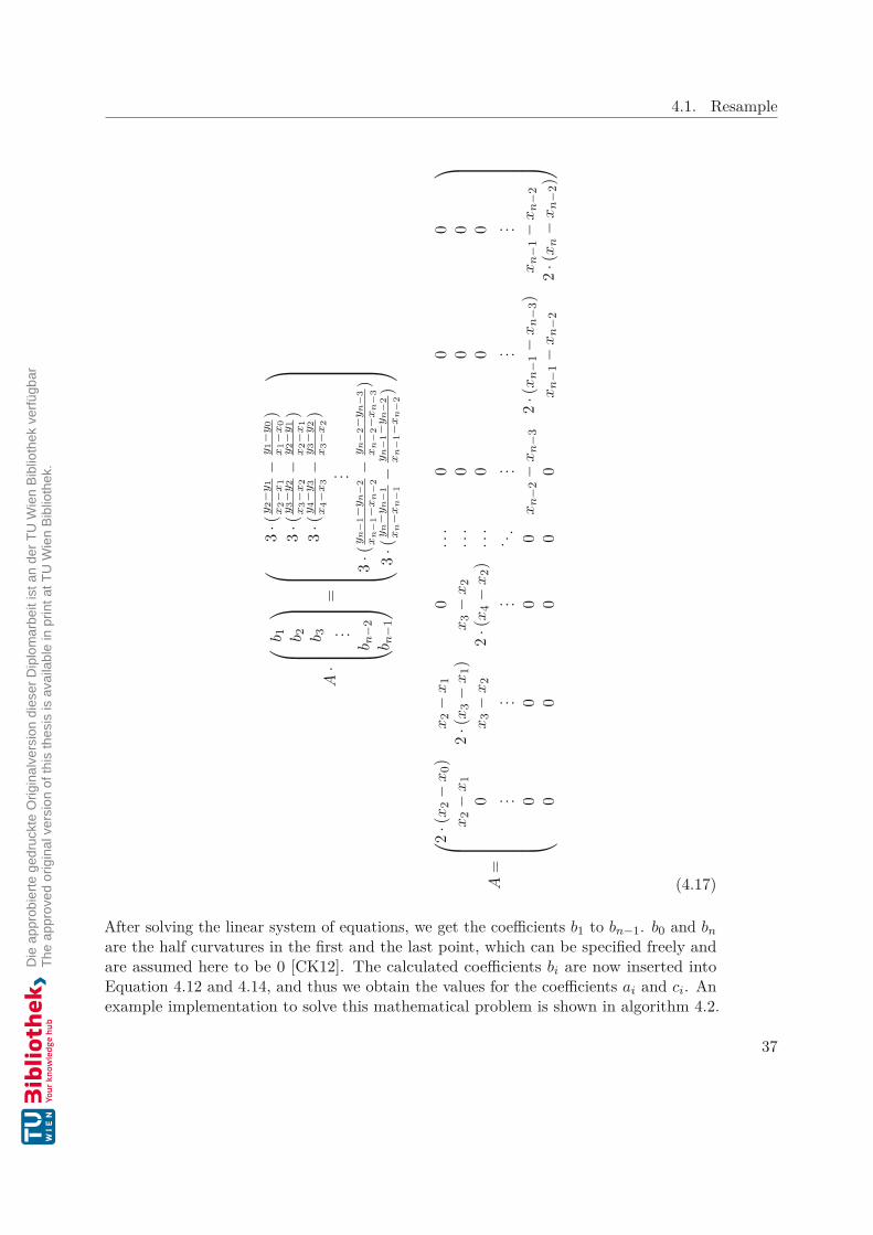
4.1. Resample

A· b 1 b 2 b 3 . . .

b n−2

b n−1

=

3·(

y2−

y1

x2−

x1

−y

1−y

0x

1−x

0)

3·(

y3−

y2

x3−

x2

−y

2−y

1x

2−x

1)

3·(

y4−

y3

x4−

x3

−y

3−y

2x

3−x

2)

. . .3

·(y

n−

1−y

n−

2x

n−

1−x

n−

2−

yn

−2−

yn

−3

xn

−2−

xn

−3)

3·(

yn

−yn

−1

xn

−xn

−1

−y

n−

1−y

n−

2x

n−

1−x

n−

2)

A=

2·(

x2

−x

0)x

2−

x1

0..

.0

00

x2

−x

12

·(x

3−

x1)

x3

−x

2..

.0

00

0x

3−

x2

2·(

x4

−x

2)..

.0

00

. . .. . .

. . .. .

.. . .

. . .. . .

00

00

xn

−2−

xn

−32

·(x

n−1

−x

n−3

)x

n−1

−x

n−2

00

00

0x

n−1

−x

n−2

2·(

xn

−x

n−2

)

(4.17)

After solving the linear system of equations, we get the coefficients b1 to bn−1. b0 and bn

are the half curvatures in the first and the last point, which can be specified freely andare assumed here to be 0 [CK12]. The calculated coefficients bi are now inserted intoEquation 4.12 and 4.14, and thus we obtain the values for the coefficients ai and ci. Anexample implementation to solve this mathematical problem is shown in algorithm 4.2.

37

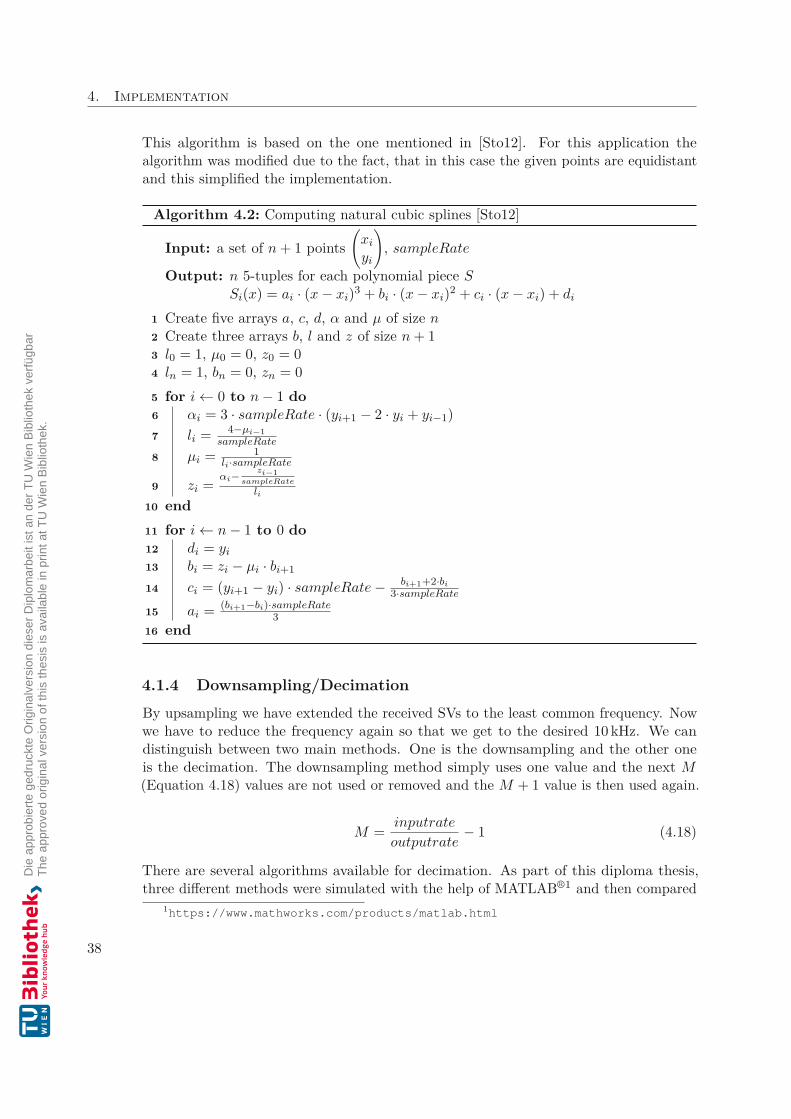
4. Implementation

This algorithm is based on the one mentioned in [Sto12]. For this application thealgorithm was modified due to the fact, that in this case the given points are equidistantand this simplified the implementation.

Algorithm 4.2: Computing natural cubic splines [Sto12]

Input: a set of n + 1 points xi

yi, sampleRate

Output: n 5-tuples for each polynomial piece SSi(x) = ai · (x − xi)3 + bi · (x − xi)2 + ci · (x − xi) + di

1 Create five arrays a, c, d, α and µ of size n2 Create three arrays b, l and z of size n + 13 l0 = 1, µ0 = 0, z0 = 04 ln = 1, bn = 0, zn = 05 for i ← 0 to n − 1 do6 αi = 3 · sampleRate · (yi+1 − 2 · yi + yi−1)7 li = 4−µi−1

sampleRate

8 µi = 1li·sampleRate

9 zi = αi− zi−1sampleRate

li

10 end11 for i ← n − 1 to 0 do12 di = yi

13 bi = zi − µi · bi+1

14 ci = (yi+1 − yi) · sampleRate − bi+1+2·bi

3·sampleRate

15 ai = (bi+1−bi)·sampleRate3

16 end

4.1.4 Downsampling/DecimationBy upsampling we have extended the received SVs to the least common frequency. Nowwe have to reduce the frequency again so that we get to the desired 10 kHz. We candistinguish between two main methods. One is the downsampling and the other oneis the decimation. The downsampling method simply uses one value and the next M(Equation 4.18) values are not used or removed and the M + 1 value is then used again.

M = inputrate

outputrate− 1 (4.18)

There are several algorithms available for decimation. As part of this diploma thesis,three different methods were simulated with the help of MATLAB®1 and then compared

1https://www.mathworks.com/products/matlab.html

38

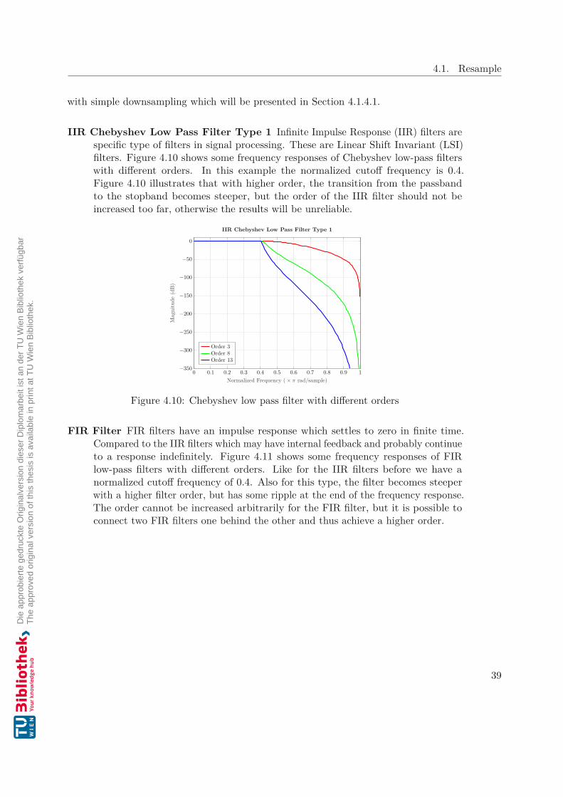
4.1. Resample

with simple downsampling which will be presented in Section 4.1.4.1.

IIR Chebyshev Low Pass Filter Type 1 Infinite Impulse Response (IIR) filters arespecific type of filters in signal processing. These are Linear Shift Invariant (LSI)filters. Figure 4.10 shows some frequency responses of Chebyshev low-pass filterswith different orders. In this example the normalized cutoff frequency is 0.4.Figure 4.10 illustrates that with higher order, the transition from the passbandto the stopband becomes steeper, but the order of the IIR filter should not beincreased too far, otherwise the results will be unreliable.

0 0.1 0.2 0.3 0.4 0.5 0.6 0.7 0.8 0.9 1−350

−300

−250

−200

−150

−100

−50

0

Normalized Frequency ( × π rad/sample)

Mag

nitu

de(d

B)

IIR Chebyshev Low Pass Filter Type 1

Order 3Order 8Order 13

Figure 4.10: Chebyshev low pass filter with different orders

FIR Filter FIR filters have an impulse response which settles to zero in finite time.Compared to the IIR filters which may have internal feedback and probably continueto a response indefinitely. Figure 4.11 shows some frequency responses of FIRlow-pass filters with different orders. Like for the IIR filters before we have anormalized cutoff frequency of 0.4. Also for this type, the filter becomes steeperwith a higher filter order, but has some ripple at the end of the frequency response.The order cannot be increased arbitrarily for the FIR filter, but it is possible toconnect two FIR filters one behind the other and thus achieve a higher order.

39

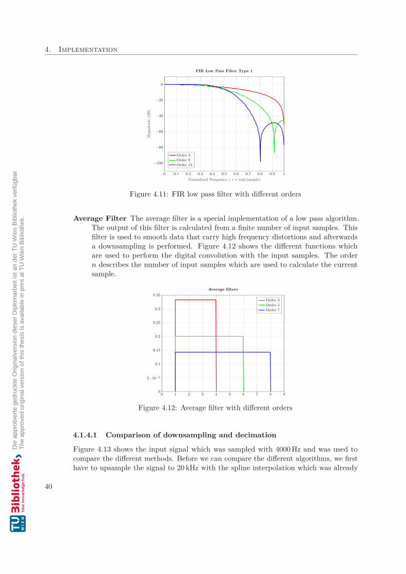
4. Implementation

0 0.1 0.2 0.3 0.4 0.5 0.6 0.7 0.8 0.9 1

−100

−80

−60

−40

−20

0

Normalized Frequency ( × π rad/sample)

Mag

nitu

de(d

B)

FIR Low Pass Filter Type 1

Order 3Order 8Order 13

Figure 4.11: FIR low pass filter with different orders

Average Filter The average filter is a special implementation of a low pass algorithm.The output of this filter is calculated from a finite number of input samples. Thisfilter is used to smooth data that carry high frequency distortions and afterwardsa downsampling is performed. Figure 4.12 shows the different functions whichare used to perform the digital convolution with the input samples. The ordern describes the number of input samples which are used to calculate the currentsample.

0 1 2 3 4 5 6 7 8 90

5 · 10−2

0.1

0.15

0.2

0.25

0.3

0.35Average filters

Order 3Order 5Order 7

Figure 4.12: Average filter with different orders

4.1.4.1 Comparison of downsampling and decimation

Figure 4.13 shows the input signal which was sampled with 4000 Hz and was used tocompare the different methods. Before we can compare the different algorithms, we firsthave to upsample the signal to 20 kHz with the spline interpolation which was already

40

4.1. Resample

described in Section 4.1.3. Now we have the same starting point for all algorithms andwe can compare the individual methods.

0 0.2 0.4 0.6 0.8 1 1.2 1.4 1.6 1.8 2·10−2

−1

−0.8

−0.6

−0.4

−0.2

0

0.2

0.4

0.6

0.8

1

t

f(t)

50Hz input signal sampled with 4000Hz

Figure 4.13: 50Hz input signal sampled with 4000Hz

First we will show the results of the IIR Chebyshev Low Pass Filter Type 1 with differentorders. The results can be found in Figure 4.14. As clearly visible, the order can have abig impact on the result. For this specific example the IIR filter with order 8 providedthe worst result in the area of the peak (Figure 4.14b) and in general the IIR filter withorder 3 had the best result and will therefore be compared with the best results of theother methods.

0 0.2 0.4 0.6 0.8 1 1.2 1.4 1.6 1.8 2·10−2

−1

−0.8

−0.6

−0.4

−0.2

0

0.2

0.4

0.6

0.8

1

t

f(t)

IIR Chebyshev Low Pass Filter Type 1

Order 3Order 8Order 13

(a) One period of the signal

4.4 4.5 4.6 4.7 4.8 4.9 5 5.1 5.2 5.3 5.4 5.5 5.6·10−3

0.986

0.988

0.99

0.992

0.994

0.996

0.998

1

t

f(t)

IIR Chebyshev Low Pass Filter Type 1

Order 3Order 8Order 13

(b) Detailed view of the peak

Figure 4.14: IIR Chebyshev Low Pass Filter Type 1 with different orders

As a next step we will use the FIR filter with different Hamming window sizes and wewill present the results in Figure 4.15. Like before we get slightly different results fordifferent Hamming window sizes. Therefore, a detailed view is shown in Figure 4.15b

41

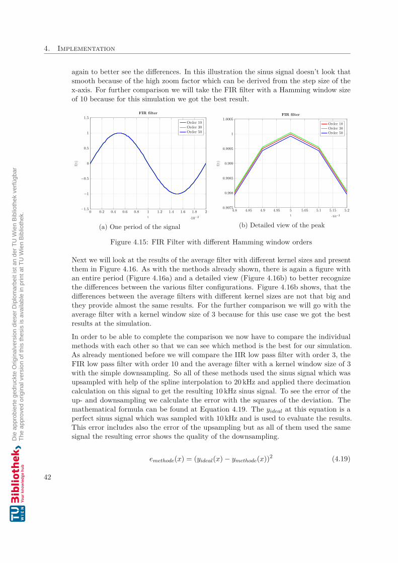
4. Implementation

again to better see the differences. In this illustration the sinus signal doesn’t look thatsmooth because of the high zoom factor which can be derived from the step size of thex-axis. For further comparison we will take the FIR filter with a Hamming window sizeof 10 because for this simulation we got the best result.

0 0.2 0.4 0.6 0.8 1 1.2 1.4 1.6 1.8 2·10−2

−1.5

−1

−0.5

0

0.5

1

1.5

t

f(t)

FIR filter

Order 10Order 30Order 50

(a) One period of the signal

4.8 4.85 4.9 4.95 5 5.05 5.1 5.15 5.2·10−3

0.9975

0.998

0.9985

0.999

0.9995

1

1.0005

tf(t

)

FIR filter

Order 10Order 30Order 50

(b) Detailed view of the peak

Figure 4.15: FIR Filter with different Hamming window orders

Next we will look at the results of the average filter with different kernel sizes and presentthem in Figure 4.16. As with the methods already shown, there is again a figure withan entire period (Figure 4.16a) and a detailed view (Figure 4.16b) to better recognizethe differences between the various filter configurations. Figure 4.16b shows, that thedifferences between the average filters with different kernel sizes are not that big andthey provide almost the same results. For the further comparison we will go with theaverage filter with a kernel window size of 3 because for this use case we got the bestresults at the simulation.

In order to be able to complete the comparison we now have to compare the individualmethods with each other so that we can see which method is the best for our simulation.As already mentioned before we will compare the IIR low pass filter with order 3, theFIR low pass filter with order 10 and the average filter with a kernel window size of 3with the simple downsampling. So all of these methods used the sinus signal which wasupsampled with help of the spline interpolation to 20 kHz and applied there decimationcalculation on this signal to get the resulting 10 kHz sinus signal. To see the error of theup- and downsampling we calculate the error with the squares of the deviation. Themathematical formula can be found at Equation 4.19. The yideal at this equation is aperfect sinus signal which was sampled with 10 kHz and is used to evaluate the results.This error includes also the error of the upsampling but as all of them used the samesignal the resulting error shows the quality of the downsampling.

emethode(x) = (yideal(x) − ymethode(x))2 (4.19)

42

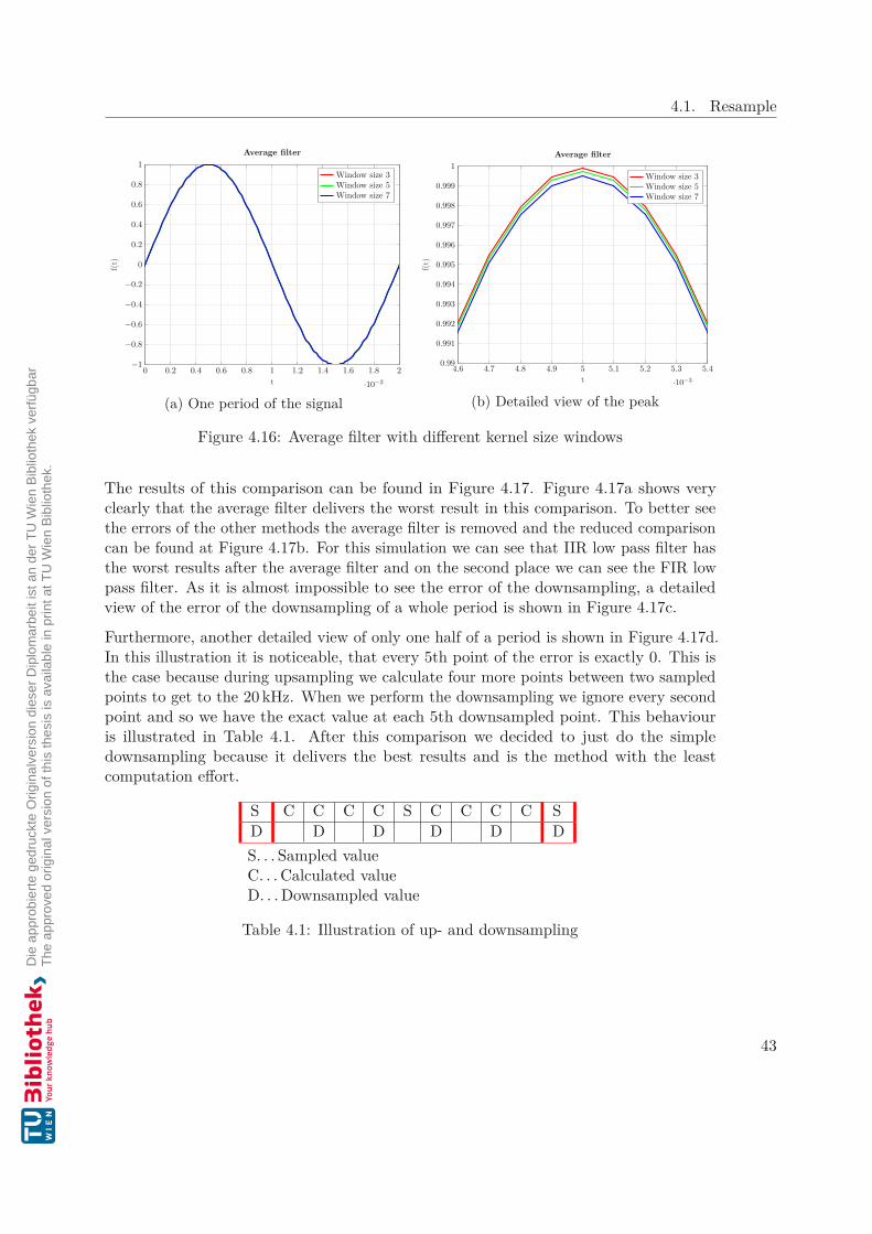
4.1. Resample

0 0.2 0.4 0.6 0.8 1 1.2 1.4 1.6 1.8 2·10−2

−1

−0.8

−0.6

−0.4

−0.2

0

0.2

0.4

0.6

0.8

1

t

f(t)

Average filter

Window size 3Window size 5Window size 7

(a) One period of the signal

4.6 4.7 4.8 4.9 5 5.1 5.2 5.3 5.4·10−3

0.99

0.991

0.992

0.993

0.994

0.995

0.996

0.997

0.998

0.999

1

t

f(t)

Average filter

Window size 3Window size 5Window size 7

(b) Detailed view of the peak

Figure 4.16: Average filter with different kernel size windows

The results of this comparison can be found in Figure 4.17. Figure 4.17a shows veryclearly that the average filter delivers the worst result in this comparison. To better seethe errors of the other methods the average filter is removed and the reduced comparisoncan be found at Figure 4.17b. For this simulation we can see that IIR low pass filter hasthe worst results after the average filter and on the second place we can see the FIR lowpass filter. As it is almost impossible to see the error of the downsampling, a detailedview of the error of the downsampling of a whole period is shown in Figure 4.17c.

Furthermore, another detailed view of only one half of a period is shown in Figure 4.17d.In this illustration it is noticeable, that every 5th point of the error is exactly 0. This isthe case because during upsampling we calculate four more points between two sampledpoints to get to the 20 kHz. When we perform the downsampling we ignore every secondpoint and so we have the exact value at each 5th downsampled point. This behaviouris illustrated in Table 4.1. After this comparison we decided to just do the simpledownsampling because it delivers the best results and is the method with the leastcomputation effort.

S C C C C S C C C C SD D D D D DS. . . Sampled valueC. . . Calculated valueD. . . Downsampled value

Table 4.1: Illustration of up- and downsampling

43

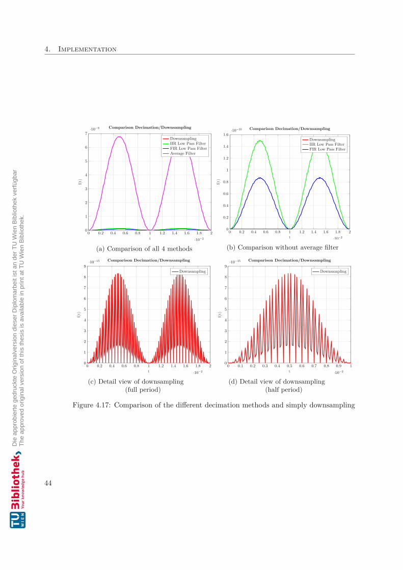
4. Implementation

0 0.2 0.4 0.6 0.8 1 1.2 1.4 1.6 1.8 2·10−2

0

1

2

3

4

5

6

7·10−9

t

f(t)

Comparison Decimation/Downsampling

DownsamplingIIR Low Pass FilterFIR Low Pass FilterAverage Filter

(a) Comparison of all 4 methods

0 0.2 0.4 0.6 0.8 1 1.2 1.4 1.6 1.8 2·10−2

0

0.2

0.4

0.6

0.8

1

1.2

1.4

1.6·10−10

t

f(t)

Comparison Decimation/Downsampling

DownsamplingIIR Low Pass FilterFIR Low Pass Filter

(b) Comparison without average filter

0 0.2 0.4 0.6 0.8 1 1.2 1.4 1.6 1.8 2·10−2

0

1

2

3

4

5

6

7

8

9·10−15

t

f(t)

Comparison Decimation/Downsampling

Downsampling

(c) Detail view of downsampling(full period)

0 0.1 0.2 0.3 0.4 0.5 0.6 0.7 0.8 0.9 1·10−2

0

1

2

3

4

5

6

7

8

9·10−15

t

f(t)

Comparison Decimation/Downsampling

Downsampling

(d) Detail view of downsampling(half period)

Figure 4.17: Comparison of the different decimation methods and simply downsampling

44

4.2. Bridge

4.2 BridgeIn this section the implementation of the so-called bridge will be explained. In Figure 4.18illustrates how the SVs are read, processed and provided to the RSE. As demonstratedin Figure 4.18, the system consists of two Soft-DSPs. Both of them consist of severalSoft-DSP executables which are executed in a periodic time.

To follow the data flow we will start to explain from the right side of Figure 4.18. Therea Frame-Buffer is illustrated which is filled by the SV socket as we already saw inFigure 2.12. This socket parses the received SV frames and provides the relevant data toFrame-Buffer. This buffer contains SVs with the specified sample rate of 4000 Hz in asubstation with 50 Hz operating frequency or 4800 Hz in a 60 Hz environment.

The first Soft-DSP executable 9 of the Digital Substation (DS) Soft-DSP reads onlyone record of the Frame-Buffer. The next executable 8 is the loop executable andcan contain several executables. For example, it could be a recorder 7 which writesthe read data to a persistent storage. This can be very useful for debugging purposes.Another executable in the loop is designed to do the upsampling calculation which wasdescribed in Subsection 4.1.3. Another one 6 is used to write the upsampled values tothe Sample-Buffer. These steps are executed over and over again and in case we havea SV stream with a sample rate of 4000 Hz we have a cycle time of ≈250 µs. The cycletime is not exactly 250 µs because this thread has to share a core of the CPU with otherthreads. This could cause, that in some cases the Soft-DSP needs a bit more time thanthe planed 250 µs. However, this is not a major problem as this thread is not part of thehard real-time condition of the system and the Frame-Buffer can compensate such issues.

The Sample-Buffer holds the upsampled values and has a sample rate of 20 kHz if theFrame-Buffer is filled with 4000 samples per second or 120 kHz if the Frame-Buffer isfilled with 4800 samples per second. This sample rate can be calculated with the leastcommon frequency which was already described with the Algorithm 4.1. The 10 kHzsample rate of the RSE is fixed and cannot be changed so the resulting sample rate of theSample-Buffer is just depending on the SV frame rate on the input. A very importantpoint in regard to this buffer is that data is written and read in real-time and thereforewe cannot use any kind of mutexes or locks. Otherwise, we could be blocked and cannotreach the 100 µs of our real-time system. Therefore, a smart ring buffer is used whichdoes not need any mutexes at all but can still recognize if data is overwritten or no data isavailable. Both of these cases should not happen in a normal run because we upsampledthe data to a common frequency but if something goes wrong an error message can beshown.

On the other side of Figure 4.18 we have the RSE Soft-DSP. As a first step 1 of everycycle, the EtherCAT frame is written. As next step the loop executable 2 , as we alreadysaw in the DS Soft-DSP, is executed. This also consists of several executables. On thisside we have an executable which reads a specific number of upsampled values. Howmany of these values are read in one cycle is as well depending on the SV frame rate.

45

4. Implementation

Since the sampling rate is higher than the 10 kHz of the RSE we have to remove someread data as described already in Subsection 4.1.4. Now we have a sample rate of 10 000samples per second and can be used for calculation purposes in other executables of theRSE Soft-DSP. On this side of the bridge we have again a recorder in place so that wecan write the up- and then downsampled values to a file and compare them with thesimulation. As a last step of every cycle, the EtherCAT frame is read. Such a cycle hasto be exactly 100 µs. As shown in Figure 4.18 we have quite some limited time to do thecalculations and therefore the up- and downsampling is simplified as much as possible sothat the newly added bridge does not disturb the already running system.

46

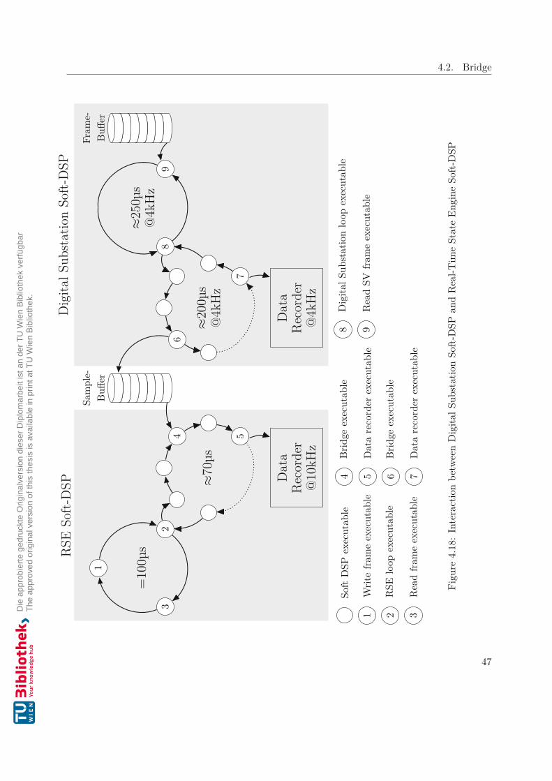
4.2. BridgeD

igita

lSub

stat

ion

Soft-

DSP

RSE

Soft-

DSP

=10

0µs

1

23

≈70µ

s

4 5

Dat

aR

ecor

der

@10

kHz

Sam

ple-

Buffe

r

≈200

µs@

4kH

z

6

7

Dat

aR

ecor

der

@4k

Hz

≈250

µs@

4kH

z8

9

Fram

e-Bu

ffer

Soft

DSP

exec

utab

le

1W

rite

fram

eex

ecut

able

2R

SElo

opex

ecut

able

3R

ead

fram

eex

ecut

able

4Br

idge

exec

utab

le

5D

ata

reco

rder

exec

utab

le

6Br

idge

exec

utab

le

7D

ata

reco

rder

exec

utab

le

8D

igita

lSub

stat

ion

loop

exec

utab

le

9R

ead

SVfra

me

exec

utab

le

Figu

re4.

18:

Inte

ract

ion

betw

een

Dig

italS

ubst

atio

nSo

ft-D

SPan

dR

eal-T

ime

Stat

eEn

gine

Soft-

DSP

47

CHAPTER 5Evaluation

In this chapter the theoretically discussed approaches are tested and evaluated on thereal device. The basic idea is to create an evaluation setup, where we can create threeanalog signals with different amplitudes which are connected to a MU. Three differentamplitudes are used to better distinguish the different channels when we analyse and plotthe data. This MU will then perform the analog to digital conversion and will providethe SVs over the Ethernet interface. These packets will then be forwarded over LAN tothe measuring device where the resampling process will be performed.

During this evaluation we will log the whole network traffic, so that we can compare thevalues which were sent form the MU and what we interpreted in our software. Basedon this data, we will analyse the behavior of the packets over time. In particular, wewill evaluate the time difference between the packets as real-time performance is a majorcriterion for this work.

Furthermore, we have also the possibility to log the values of the output signals and theinput signals before resampling as well as after resampling. This allows us to evaluate thecorrectness of our Bridge. In addition to this correctness, we also must check that thisadditional Bridge has no negative influence on the already existing hard real-time system.Some timing information of the RSE Soft-DSP thread and the DS Soft-DSP thread islogged after each execution and can be also analysed. If the real-time condition could nothold during execution we would anyways get an exception and the execution would stop.

5.1 Evaluation setupFigure 5.1 shows the evaluation setup which was used to check the implementation onthe running system. As illustrated in Figure 5.1, we simplified the setup a bit comparedto the one shown in Figure 2.10. This decision was taken because for testing the system

49

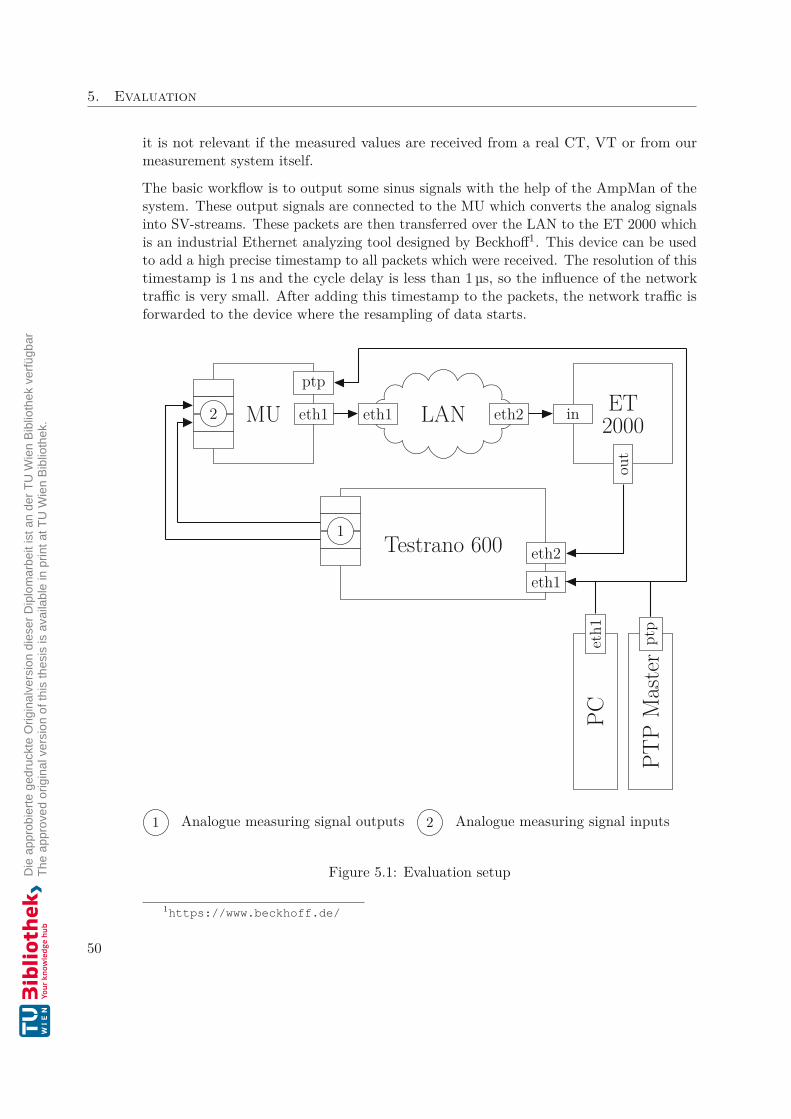
5. Evaluation

it is not relevant if the measured values are received from a real CT, VT or from ourmeasurement system itself.

The basic workflow is to output some sinus signals with the help of the AmpMan of thesystem. These output signals are connected to the MU which converts the analog signalsinto SV-streams. These packets are then transferred over the LAN to the ET 2000 whichis an industrial Ethernet analyzing tool designed by Beckhoff1. This device can be usedto add a high precise timestamp to all packets which were received. The resolution of thistimestamp is 1 ns and the cycle delay is less than 1 µs, so the influence of the networktraffic is very small. After adding this timestamp to the packets, the network traffic isforwarded to the device where the resampling of data starts.

Testrano 600eth1

eth21

LANeth1 eth2MU eth1

ptp

2 ET2000in

out

PCet

h1

PTP

Mas

ter

ptp

1 Analogue measuring signal outputs 2 Analogue measuring signal inputs

Figure 5.1: Evaluation setup

1https://www.beckhoff.de/

50

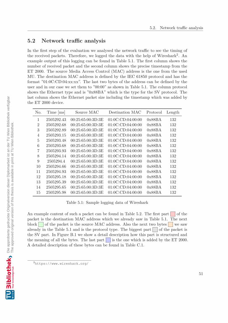
5.2. Network traffic analysis

5.2 Network traffic analysisIn the first step of the evaluation we analysed the network traffic to see the timing ofthe received packets. Therefore, we logged the data with the help of Wireshark2. Anexample output of this logging can be found in Table 5.1. The first column shows thenumber of received packet and the second column shows the precise timestamp from theET 2000. The source Media Access Control (MAC) address is the one from the usedMU. The destination MAC address is defined by the IEC 61850 protocol and has theformat ”01:0C:CD:04:xx:xx”. The last two bytes of the address can be defined by theuser and in our case we set them to ”00:00” as shown in Table 5.1. The column protocolshows the Ethernet type and is ”0x88BA” which is the type for the SV protocol. Thelast column shows the Ethernet packet size including the timestamp which was added bythe ET 2000 device.

No. Time [ms] Source MAC Destination MAC Protocol Length1 2505292.43 00:25:65:00:3D:3E 01:0C:CD:04:00:00 0x88BA 1322 2505292.68 00:25:65:00:3D:3E 01:0C:CD:04:00:00 0x88BA 1323 2505292.89 00:25:65:00:3D:3E 01:0C:CD:04:00:00 0x88BA 1324 2505293.15 00:25:65:00:3D:3E 01:0C:CD:04:00:00 0x88BA 1325 2505293.48 00:25:65:00:3D:3E 01:0C:CD:04:00:00 0x88BA 1326 2505293.68 00:25:65:00:3D:3E 01:0C:CD:04:00:00 0x88BA 1327 2505293.93 00:25:65:00:3D:3E 01:0C:CD:04:00:00 0x88BA 1328 2505294.14 00:25:65:00:3D:3E 01:0C:CD:04:00:00 0x88BA 1329 2505294.4 00:25:65:00:3D:3E 01:0C:CD:04:00:00 0x88BA 13210 2505294.66 00:25:65:00:3D:3E 01:0C:CD:04:00:00 0x88BA 13211 2505294.93 00:25:65:00:3D:3E 01:0C:CD:04:00:00 0x88BA 13212 2505295.18 00:25:65:00:3D:3E 01:0C:CD:04:00:00 0x88BA 13213 2505295.39 00:25:65:00:3D:3E 01:0C:CD:04:00:00 0x88BA 13214 2505295.65 00:25:65:00:3D:3E 01:0C:CD:04:00:00 0x88BA 13215 2505295.98 00:25:65:00:3D:3E 01:0C:CD:04:00:00 0x88BA 132

Table 5.1: Sample logging data of Wireshark

An example content of such a packet can be found in Table 5.2. The first part of thepacket is the destination MAC address which we already saw in Table 5.1. The nextblock of the packet is the source MAC address. Also the next two bytes we sawalready in the Table 5.1 and is the protocol type. The biggest part of the packet isthe SV part. In Figure B.1 we show a detail description how this part is structured andthe meaning of all the bytes. The last part is the one which is added by the ET 2000.A detailed description of these bytes can be found in Table C.1.

2https://www.wireshark.org/

51

5. Evaluation

01 0C CD 04 00 00 00 25 65 00 3D 3E 88 BA 40 0000 66 00 00 00 00 60 5C 80 01 01 A2 57 30 55 8004 34 30 30 30 82 02 07 61 83 04 00 00 00 01 8501 02 87 40 FF FF FF EF 00 00 00 00 FF FF FF C300 00 00 00 FF FF FF F7 00 00 00 00 FF FF FF CC00 00 00 00 00 00 00 00 00 00 00 00 FF FF FF FD00 00 00 00 00 00 00 03 00 00 00 00 00 00 00 0300 00 00 00 01 01 05 10 00 00 80 00 F0 A7 10 4F47 02 00 00

Table 5.2: Example content of an Ethernet packet

5.3 Packet timing analysisAfter checking the content of the Ethernet packets we decided to use this additionaldata from the ET 2000 and analyse the timing of the packets. Especially the timedifference between two SV packets. With the help of Wireshark3 we therefore loggedabout 1 000 000 SV packets which is a bit more than 4 min. The distribution of the timedifferences can be found in Figure 5.2. As illustrated the time difference of ≈ 60 % of thereceived packets were in the range of 235 µs to 265 µs. Furthermore, Figure 5.2 showsthat ≈ 20 % were received even faster and ≈ 10 % had a time difference of more than300 µs. Because of these packets which take significantly longer than the expected 250 µs,we decided to buffer a certain number of packets at the Frame-Buffer of Figure 4.18before we start with resampling so that we have at any point of the execution enoughelements in the Frame-Buffer. If we would run out of elements we would not be able todo the resampling which has the consequence that the Sample-Buffer of Figure 4.18 willget empty and the RSE will fail because it expects that in each loop it can read a valuefrom the Sample-Buffer. This initial delay is not a big problem, because the delay can bederived from the initial number of elements in the Frame-Buffer and is constant for allexecutions. For future calculation it is important to know this delay because every delayfrom outputting a signal until receiving the measured value will result in a measurementerror.

3https://www.wireshark.org/

52

5.4. Analysis of the output and input signals

200 250 3000 %

5 %

10 %

15 %

20 %

25 %

30 %

35 %

40 %

45 %

50 %

t in µs

Pack

ets

inea

chtim

egr

oup

of10

µsTime difference between the received SV packets

Figure 5.2: Distribution of time differences between received SV packets

5.4 Analysis of the output and input signalsAs a next step the output signal of the AmpMan of the measuring device is loggedand displayed in Figure 5.3. This signal was calculated by the Soft-DSP and is thentransferred to the AmpMan. The logging starts a bit earlier then the calculation of theoutput signal, therefore there is a small delay of about 130 ms in Figure 5.3. So that theindividual three voltages can be better distinguished, different amplitudes were used forthe sine signals. For Output Voltage A we used a peak amplitude of about 70 V which isshown in Figure 5.3a. The top signal shows a bigger time range and the bottom signalsshows only a part of the top signal to better see the signal. For Output Voltage B andOutput Voltage C we used a peak amplitude of 80 V and 100 V as shown in Figure 5.3band Figure 5.3c. After approximately 3 s the thread of the RSE was stopped and thedata were written to the log file. All these output data were recorded at a frequency of10 kHz with the data recorder executable 5 which was already shown in Figure 4.18.

53

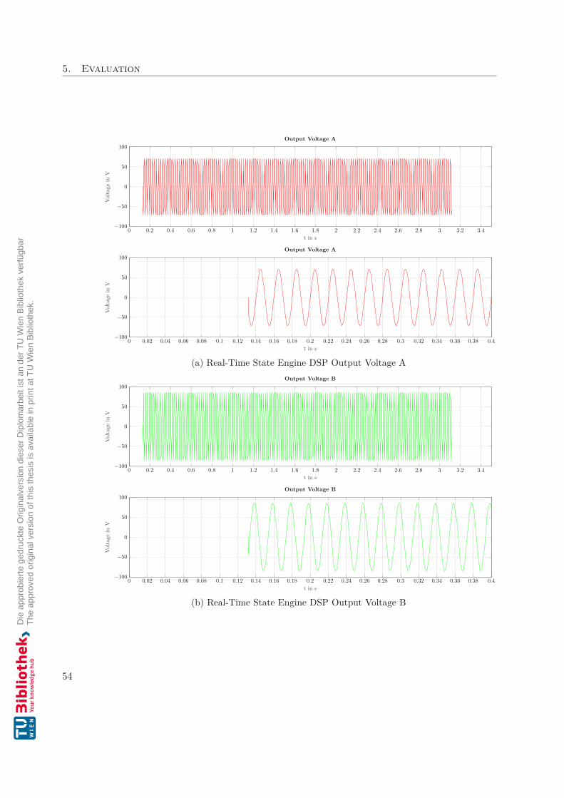
5. Evaluation

0 0.2 0.4 0.6 0.8 1 1.2 1.4 1.6 1.8 2 2.2 2.4 2.6 2.8 3 3.2 3.4−100

−50

0

50

100

t in s

Volta

gein

V

Output Voltage A

0 0.02 0.04 0.06 0.08 0.1 0.12 0.14 0.16 0.18 0.2 0.22 0.24 0.26 0.28 0.3 0.32 0.34 0.36 0.38 0.4−100

−50

0

50

100

t in s

Volta

gein

V

Output Voltage A

(a) Real-Time State Engine DSP Output Voltage A

0 0.2 0.4 0.6 0.8 1 1.2 1.4 1.6 1.8 2 2.2 2.4 2.6 2.8 3 3.2 3.4−100

−50

0

50

100

t in s

Volta

gein

V

Output Voltage B

0 0.02 0.04 0.06 0.08 0.1 0.12 0.14 0.16 0.18 0.2 0.22 0.24 0.26 0.28 0.3 0.32 0.34 0.36 0.38 0.4−100

−50

0

50

100

t in s

Volta

gein

V

Output Voltage B

(b) Real-Time State Engine DSP Output Voltage B

54

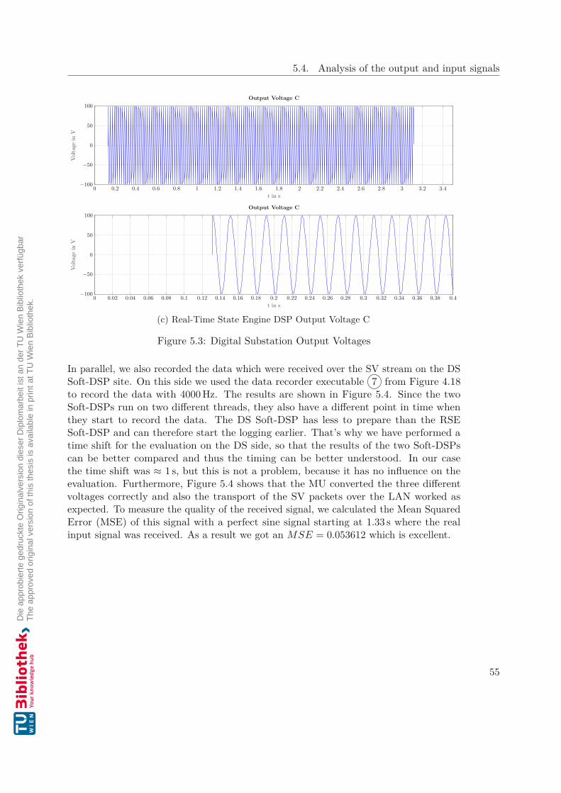
5.4. Analysis of the output and input signals

0 0.2 0.4 0.6 0.8 1 1.2 1.4 1.6 1.8 2 2.2 2.4 2.6 2.8 3 3.2 3.4−100

−50

0

50

100

t in s

Volta

gein

V

Output Voltage C

0 0.02 0.04 0.06 0.08 0.1 0.12 0.14 0.16 0.18 0.2 0.22 0.24 0.26 0.28 0.3 0.32 0.34 0.36 0.38 0.4−100

−50

0

50

100

t in s

Volta

gein

V

Output Voltage C

(c) Real-Time State Engine DSP Output Voltage C

Figure 5.3: Digital Substation Output Voltages

In parallel, we also recorded the data which were received over the SV stream on the DSSoft-DSP site. On this side we used the data recorder executable 7 from Figure 4.18to record the data with 4000 Hz. The results are shown in Figure 5.4. Since the twoSoft-DSPs run on two different threads, they also have a different point in time whenthey start to record the data. The DS Soft-DSP has less to prepare than the RSESoft-DSP and can therefore start the logging earlier. That’s why we have performed atime shift for the evaluation on the DS side, so that the results of the two Soft-DSPscan be better compared and thus the timing can be better understood. In our casethe time shift was ≈ 1 s, but this is not a problem, because it has no influence on theevaluation. Furthermore, Figure 5.4 shows that the MU converted the three differentvoltages correctly and also the transport of the SV packets over the LAN worked asexpected. To measure the quality of the received signal, we calculated the Mean SquaredError (MSE) of this signal with a perfect sine signal starting at 1.33 s where the realinput signal was received. As a result we got an MSE = 0.053612 which is excellent.

55

5. Evaluation

0 0.2 0.4 0.6 0.8 1 1.2 1.4 1.6 1.8 2 2.2 2.4 2.6 2.8 3 3.2 3.4−100

−50

0

50

100

t in s

Volta

gein

V

Input Voltage A

1.2 1.22 1.24 1.26 1.28 1.3 1.32 1.34 1.36 1.38 1.4 1.42 1.44 1.46 1.48 1.5 1.52 1.54 1.56 1.58 1.6−100

−50

0

50

100

t in s

Volta

gein

V

Input Voltage A

(a) Digital Substation DSP Input Voltage A

0 0.2 0.4 0.6 0.8 1 1.2 1.4 1.6 1.8 2 2.2 2.4 2.6 2.8 3 3.2 3.4−100

−50

0

50

100

t in s

Volta

gein

V

Input Voltage B

1.2 1.22 1.24 1.26 1.28 1.3 1.32 1.34 1.36 1.38 1.4 1.42 1.44 1.46 1.48 1.5 1.52 1.54 1.56 1.58 1.6−100

−50

0

50

100

t in s

Volta

gein

V

Input Voltage B

(b) Digital Substation DSP Input Voltage B

56

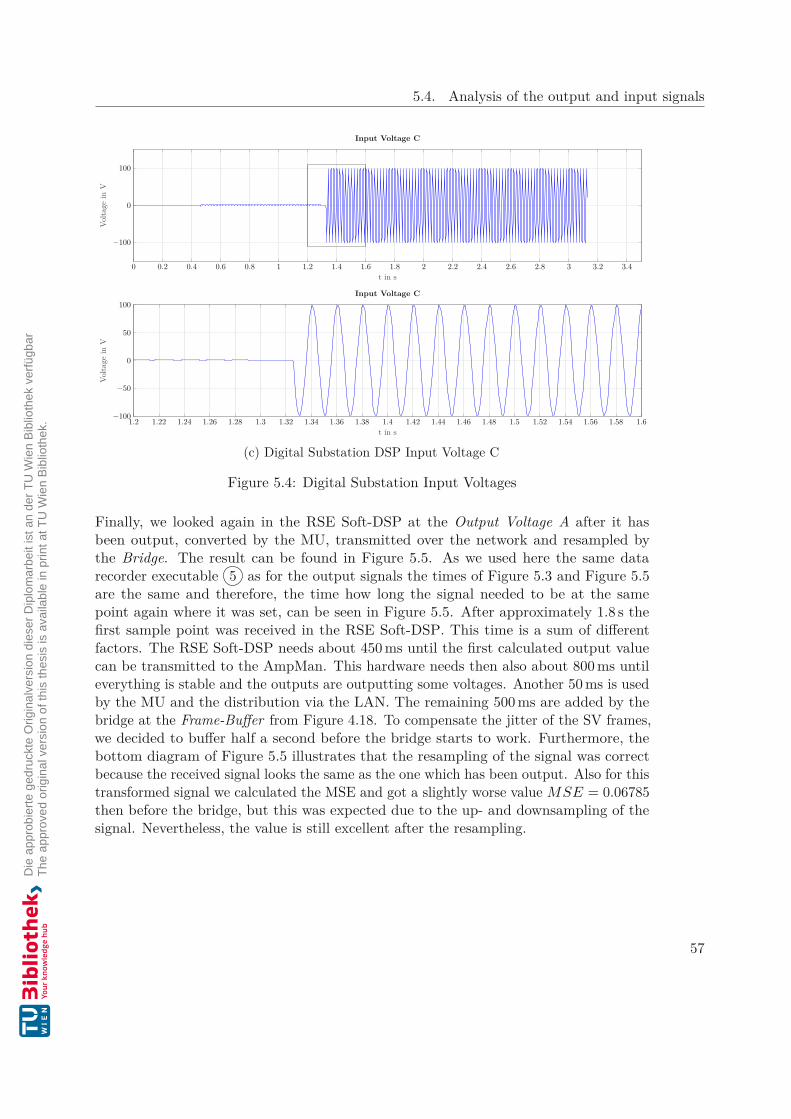
5.4. Analysis of the output and input signals

0 0.2 0.4 0.6 0.8 1 1.2 1.4 1.6 1.8 2 2.2 2.4 2.6 2.8 3 3.2 3.4

−100

0

100

t in s

Volta

gein

V

Input Voltage C

1.2 1.22 1.24 1.26 1.28 1.3 1.32 1.34 1.36 1.38 1.4 1.42 1.44 1.46 1.48 1.5 1.52 1.54 1.56 1.58 1.6−100

−50

0

50

100

t in s

Volta

gein

V

Input Voltage C

(c) Digital Substation DSP Input Voltage C

Figure 5.4: Digital Substation Input Voltages

Finally, we looked again in the RSE Soft-DSP at the Output Voltage A after it hasbeen output, converted by the MU, transmitted over the network and resampled bythe Bridge. The result can be found in Figure 5.5. As we used here the same datarecorder executable 5 as for the output signals the times of Figure 5.3 and Figure 5.5are the same and therefore, the time how long the signal needed to be at the samepoint again where it was set, can be seen in Figure 5.5. After approximately 1.8 s thefirst sample point was received in the RSE Soft-DSP. This time is a sum of differentfactors. The RSE Soft-DSP needs about 450 ms until the first calculated output valuecan be transmitted to the AmpMan. This hardware needs then also about 800 ms untileverything is stable and the outputs are outputting some voltages. Another 50 ms is usedby the MU and the distribution via the LAN. The remaining 500 ms are added by thebridge at the Frame-Buffer from Figure 4.18. To compensate the jitter of the SV frames,we decided to buffer half a second before the bridge starts to work. Furthermore, thebottom diagram of Figure 5.5 illustrates that the resampling of the signal was correctbecause the received signal looks the same as the one which has been output. Also for thistransformed signal we calculated the MSE and got a slightly worse value MSE = 0.06785then before the bridge, but this was expected due to the up- and downsampling of thesignal. Nevertheless, the value is still excellent after the resampling.

57

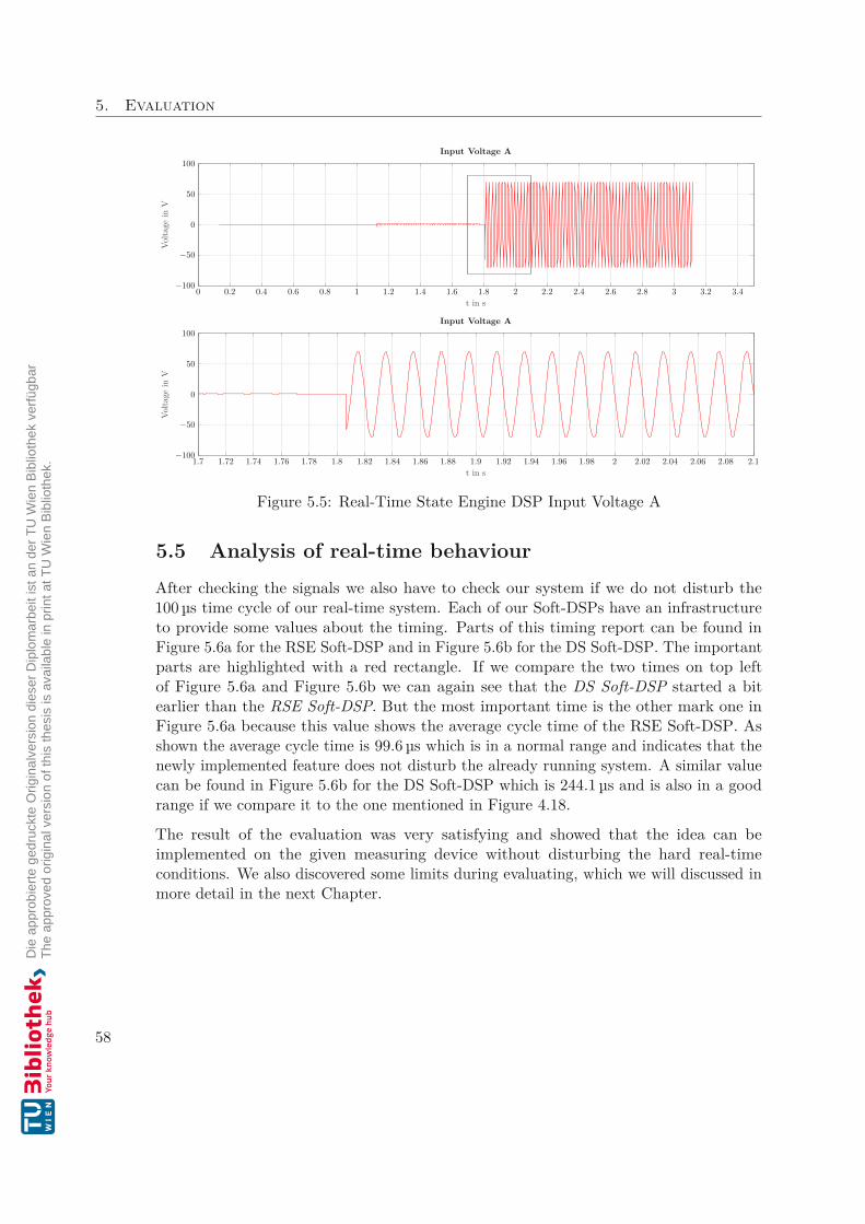
5. Evaluation

0 0.2 0.4 0.6 0.8 1 1.2 1.4 1.6 1.8 2 2.2 2.4 2.6 2.8 3 3.2 3.4−100

−50

0

50

100

t in s

Volta

gein

VInput Voltage A

1.7 1.72 1.74 1.76 1.78 1.8 1.82 1.84 1.86 1.88 1.9 1.92 1.94 1.96 1.98 2 2.02 2.04 2.06 2.08 2.1−100

−50

0

50

100

t in s

Volta

gein

V

Input Voltage A

Figure 5.5: Real-Time State Engine DSP Input Voltage A

5.5 Analysis of real-time behaviourAfter checking the signals we also have to check our system if we do not disturb the100 µs time cycle of our real-time system. Each of our Soft-DSPs have an infrastructureto provide some values about the timing. Parts of this timing report can be found inFigure 5.6a for the RSE Soft-DSP and in Figure 5.6b for the DS Soft-DSP. The importantparts are highlighted with a red rectangle. If we compare the two times on top leftof Figure 5.6a and Figure 5.6b we can again see that the DS Soft-DSP started a bitearlier than the RSE Soft-DSP. But the most important time is the other mark one inFigure 5.6a because this value shows the average cycle time of the RSE Soft-DSP. Asshown the average cycle time is 99.6 µs which is in a normal range and indicates that thenewly implemented feature does not disturb the already running system. A similar valuecan be found in Figure 5.6b for the DS Soft-DSP which is 244.1 µs and is also in a goodrange if we compare it to the one mentioned in Figure 4.18.

The result of the evaluation was very satisfying and showed that the idea can beimplemented on the given measuring device without disturbing the hard real-timeconditions. We also discovered some limits during evaluating, which we will discussed inmore detail in the next Chapter.

58

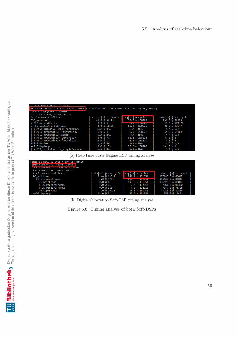
5.5. Analysis of real-time behaviour

(a) Real-Time State Engine DSP timing analyse

(b) Digital Substation Soft-DSP timing analyse

Figure 5.6: Timing analyse of both Soft-DSPs

59

CHAPTER 6Conclusion and Future Work

In the previous Chapter 5 we already saw that the idea of this thesis is working withoutdisturbing the already running real-time system. Nevertheless, we faced some issuesduring the evaluation and found some limits for the current implementation which willbe discussed in the first part of this chapter. After that the future work and how thisimplementation can be extended will be described.

During the first runs we noticed that the Frame buffer from Figure 4.18 was often emptyand therefore the system stopped, which should not happen under any circumstances. Asalready described in Chapter 5 and shown in Figure 5.2 we found out, that approximately20 % of all received packets were late. Furthermore, we could see in Wireshark1 thatthe time difference of the time stamp added from the program is not constant to theone added from the ET 2000. After some investigation we found out, that dependingon the Ethernet interface settings the operating system handles the interrupt behaviourof the received packets differently. It can happen that the operating system bufferssome frames and just sends a single interrupt for multiple packets. With this knowledgewe changed the settings that there is an interrupt for every received packet as soon aspossible so that the DS Soft-DSP can process the packets faster and that there is noadditional delay. The big disadvantage of one interrupt per packet is that the CPUworkload gets increased significantly. This hardly has any effect on a powerful CPUbut on our system there is a P20202 with only two cores with a clock frequency up to1.2 GHz installed. Furthermore, one of these two cores is as good as possible isolatedand is only used by the RSE Soft-DSP so that the hard real-time conditions can beachieved. The second core is shared for all other activities and is therefore very busyand a modification of the interrupt handling has a big influence on the performance ofthis second core. Nevertheless, we decided to go for this modification because the systemcould handle this overhead. To compensate the variety of the time differences between

1https://www.wireshark.org/2https://www.nxp.com/docs/en/fact-sheet/QP20XXFS.pdf

61

6. Conclusion and Future Work

the packets we decided to wait at the beginning of the execution until the Frame-Bufferof Figure 4.18 has a specific number stored. With this two changes we were able to getthe results shown in Chapter 5.

Further we found out, that we can not resample all the signals which we received overthe SV packets. As shown in Figure B.3 a single SV packet would include four voltagesand four currents. One for each phase and one for the neutral. As already describedin Chapter 5 we only resampled the Output Voltage A and forwarded this informationto the RSE Soft-DSP. This was done because when we tried to do all eight signals thesystem was overwhelmed and the execution was stopped. In principle the implementationwould work for all eight signals if there would be a more powerful CPU in place.

Overall the aim of the thesis could be met and all the problems described in Section 1.1could be solved. We could show in this thesis how to exchange data between twoindependent threads which are running on different clock rates without disturbing analready running hard real-time system.

This brings us to a possible expansion in the future. The measuring device will be revisedand will then get a more powerful CPU with more cores. Similar to the RSE Soft-DSPthe DS Soft-DSP will then also get an isolated core and then the performance issueswill be gone and all the eight channels can be resampled. Furthermore, we will get acycle time closer to 250 µs for the DS Soft-DSP and therefore also a better result of theresampled signal.

Currently, we just provide the resampled signals to the RSE Soft-DSP but the data isnot used yet. An extension to this work is to use these data and do the same calculationsas already done with the conventional converters and analog signals. Another possibleextension could be to evaluate the received data immediately and to change the outputsof the measuring device based on the received data. For this expansion we would alsoneed the more powerful CPU and we would have to keep all possible delays in the chainas small as possible. This would, however, have been beyond the scope of the thesis.

62

APPENDIX AIEC 61850 Parts

Part Title Ver. Date

1 TR Introduction and overview 2.0 03/20132 TS Glossary 2.0 04/20193 General requirements 2.0 12/20134 System and project management 2.0 04/20115 Communication requirements for functions and device models 2.0 01/2013

6 Configuration description language for communication inpower utility automation systems related to IEDs 2.1 06/2018

7-1 Basic communication structure - Principles and models 2.0 07/2011

7-2 Basic information and communication structure - Abstractcommunication service interface (ACSI) 2.0 08/2010

7-3 Basic communication structure - Common data classes 2.0 12/2010

7-4 Basic communication structure - Compatible logical nodeclasses and data object classes 2.0 03/2010

7-6 TR Guideline for definition of Basic Application Profiles (BAPs)using IEC 61850 1.0 01/2019

7-7 TS Machine-processable format of IEC 61850-related data modelsfor tools 1.0 03/2018

7-410 Basic communication structure - Hydroelectricpower plants -Communication for monitoring and control 2.1 11/2015

7-420 Basic communication structure - Distributed energyresources logical nodes 1.0 03/2009

7-500 TRBasic information and communication structure - Use oflogical nodes for modeling application functions and relatedconcepts and guidelines for substations

1.0 07/2017

7-510 TR Basic communication structure - Hydroelectric powerplants -Modelling concepts and guidelines 1.0 03/2012

8-1 Specific communication service mapping (SCSM) - Mappingsto MMS (ISO 9506-1, ISO 9506-2) and to ISO/IEC 8802-3 2.0 06/2011

63

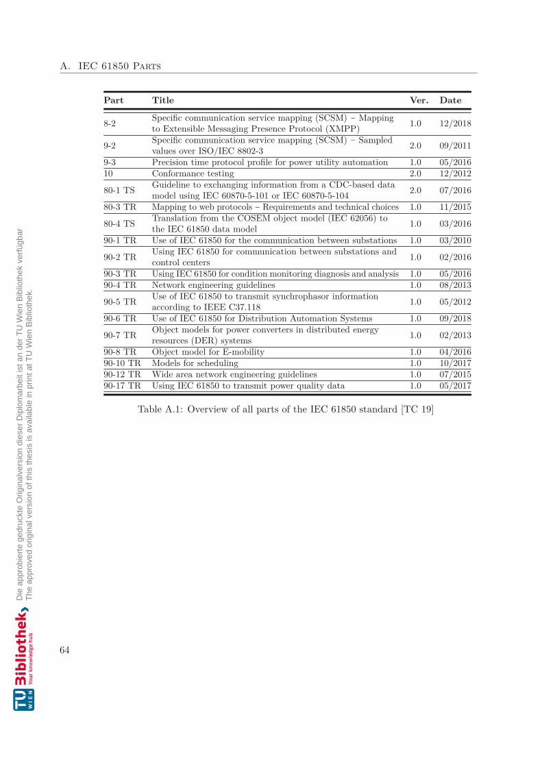
A. IEC 61850 Parts

Part Title Ver. Date

8-2 Specific communication service mapping (SCSM) - Mappingto Extensible Messaging Presence Protocol (XMPP) 1.0 12/2018

9-2 Specific communication service mapping (SCSM) - Sampledvalues over ISO/IEC 8802-3 2.0 09/2011

9-3 Precision time protocol profile for power utility automation 1.0 05/201610 Conformance testing 2.0 12/2012

80-1 TS Guideline to exchanging information from a CDC-based datamodel using IEC 60870-5-101 or IEC 60870-5-104 2.0 07/2016

80-3 TR Mapping to web protocols - Requirements and technical choices 1.0 11/2015

80-4 TS Translation from the COSEM object model (IEC 62056) tothe IEC 61850 data model 1.0 03/2016

90-1 TR Use of IEC 61850 for the communication between substations 1.0 03/2010

90-2 TR Using IEC 61850 for communication between substations andcontrol centers 1.0 02/2016

90-3 TR Using IEC 61850 for condition monitoring diagnosis and analysis 1.0 05/201690-4 TR Network engineering guidelines 1.0 08/2013

90-5 TR Use of IEC 61850 to transmit synchrophasor informationaccording to IEEE C37.118 1.0 05/2012

90-6 TR Use of IEC 61850 for Distribution Automation Systems 1.0 09/2018

90-7 TR Object models for power converters in distributed energyresources (DER) systems 1.0 02/2013

90-8 TR Object model for E-mobility 1.0 04/201690-10 TR Models for scheduling 1.0 10/201790-12 TR Wide area network engineering guidelines 1.0 07/201590-17 TR Using IEC 61850 to transmit power quality data 1.0 05/2017

Table A.1: Overview of all parts of the IEC 61850 standard [TC 19]

64

APPENDIX BContent of an IEC 61850-9-2-LE

Ethernet frame

Figure B.1 shows the content of a IEC 61850-9-2-LE Ethernet frame. The APDU fieldmentioned in this figure is then shown in more detail in Figure B.2. The Sequence ofData field of Figure B.2 is then described in Figure B.3.

Figure B.1 remarks [UCA11]

• Data fields with a length of 1 byte have the Most Significant Bit (MSB) on the leftside and the Least Significant Bit (LSB) on the right side.

• Data fields longer than 1 byte have the MSB at the top left and the LSB at thebottom right, as shown in the “Preamble” data field.

• Sending bytes, bit 1 is the first bit.

65

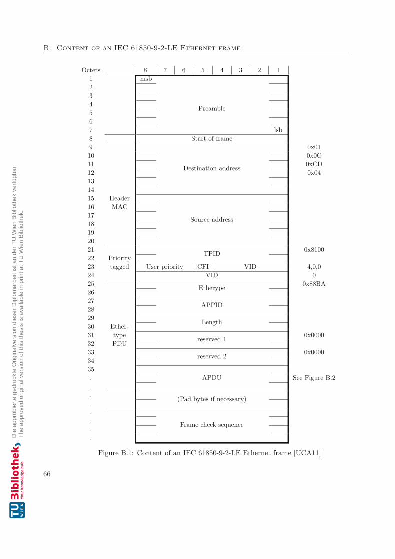
B. Content of an IEC 61850-9-2-LE Ethernet frame

Octets 8 7 6 5 4 3 2 11 msb mss mss mss mss mss mss mss2

Preamble

34567 lsb8 Start of frame9

Destination address

0x0110 0x0C11 0xCD12 0x04131415 Header

Source address

16 MAC1718192021 TPID 0x810022 Priority23 tagged User priority CFI VID 4,0,024 VID 025 Etherype 0x88BA2627 APPID2829 Length30 Ether-31 type reserved 1 0x000032 PDU33 reserved 2 0x00003435

APDU. See Figure B.2.. (Pad bytes if necessary)..

Frame check sequence...

Figure B.1: Content of an IEC 61850-9-2-LE Ethernet frame [UCA11]

66

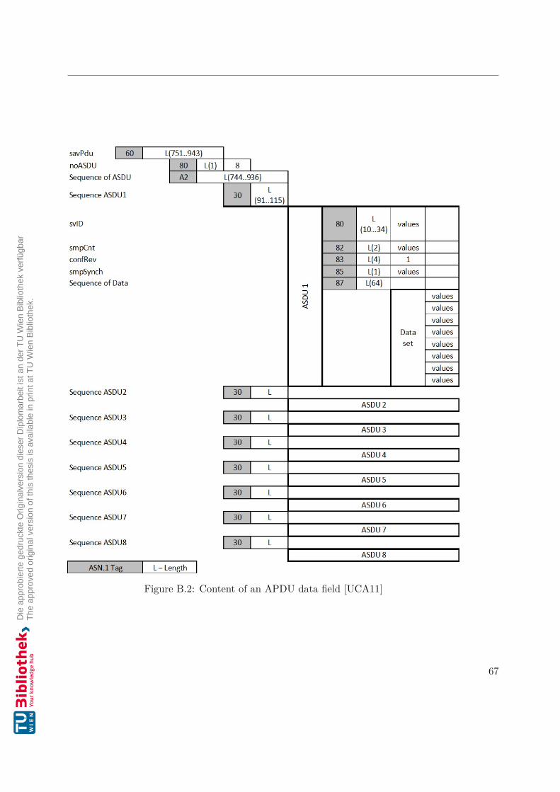
Figure B.2: Content of an APDU data field [UCA11]

67

B. Content of an IEC 61850-9-2-LE Ethernet frame

8 7 6 5 4 3 2 1msb

InnATCTR1.Amp.instMag.ilsb

InnATCTR1.Amp.qder OpB Test Source DetailQual

DetailQual validity

InnBTCTR2.Amp.instMag.i

InnBTCTR2.Amp.q

InnCTCTR3.Amp.instMag.i

InnCTCTR3.Amp.q

InnNmTCTR4.Amp.instMag.i

InnNmTCTR4.Amp.q

UnnATVTR1.Vol.instMag.i

UnnATVTR1.Vol.q

UnnBTVTR2.Vol.instMag.i

UnnBTVTR2.Vol.q

UnnCTVTR3.Vol.instMag.i

UnnCTVTR3.Vol.q

UnnNmTVTR4.Vol.instMag.i

UnnNmTVTR1.Vol.q

Figure B.3: Encoding of dataset [UCA11]

68

APPENDIX CContent of the additional

ET 2000 packet data

6 Bytes Identifier 01 01 05 10 00 00(symbolic MAC address)

1 Byte

Port designation 0. . . 7 of arriving framePort Hex BinX1.0 0x80 10000000X1.1 0x40 01000000X2.0 0x20 00100000X2.1 0x10 00010000X3.0 0x08 00001000X3.1 0x04 00000100X4.0 0x02 00000010X4.1 0x01 00000001

1 Byte

Bits 0. . . 2 reservedBit 3 alignment errorBit 4 CRC error in recorded frameBits 5. . . 7 unused

8 Bytes Timestamp in ns(reading direction backwards)

Table C.1: Constitution of the 16 additional bytes of the ET 2000

69

List of Figures

1.1 Measuring setup for a conventional instrument transformer . . . . . . . . 21.2 Measuring setup for a NCIT . . . . . . . . . . . . . . . . . . . . . . . . . . 31.3 Thread overview of the measuring device . . . . . . . . . . . . . . . . . . 4

2.1 Electric power system overview [Blu07] . . . . . . . . . . . . . . . . . . . . 82.2 Monitoring and controlling of an electric power system [Gö14] . . . . . . . 92.3 Overview of IEC 61850 three main topics: 1 Modelling, 2 Configuration,

3 Communication [PA18] . . . . . . . . . . . . . . . . . . . . . . . . . . . 112.4 Example of a logical node for a non-phase related measurement [SSA+11] 122.5 IEEE 1588 protocol message exchange pattern [MML+16]. . . . . . . . . . 152.6 EtherCAT topology with branches [WB05] . . . . . . . . . . . . . . . . . 162.7 Two different EtherCAT slave types [WB05] . . . . . . . . . . . . . . . . . 172.8 EtherCAT telegram structure [WB05] . . . . . . . . . . . . . . . . . . . . 172.9 TESTRANO 600 [OMI19] . . . . . . . . . . . . . . . . . . . . . . . . . . . 182.10 Possible experimental setup for this diploma thesis . . . . . . . . . . . . . 202.11 Core modules of the TESTRANO 600 . . . . . . . . . . . . . . . . . . . . . 212.12 Core modules of the system . . . . . . . . . . . . . . . . . . . . . . . . . . 22

3.1 Illustration of SRS system in a protection IED [CY10] . . . . . . . . . . . 233.2 A new digital system with EITs, Big MU and IEDs [TJW11] . . . . . . . 253.3 Sampling rate conversion [TJW11] . . . . . . . . . . . . . . . . . . . . . . 253.4 Block diagram of the ALSS resampler [PT16] . . . . . . . . . . . . . . . . 263.5 Program structure of the resampling process [CMSdR20] . . . . . . . . . . 27

4.1 Previous Neighbor . . . . . . . . . . . . . . . . . . . . . . . . . . . . . . . 304.2 Next Neighbor . . . . . . . . . . . . . . . . . . . . . . . . . . . . . . . . . 304.3 Nearest Neighbor . . . . . . . . . . . . . . . . . . . . . . . . . . . . . . . . . 314.4 Linear Interpolation . . . . . . . . . . . . . . . . . . . . . . . . . . . . . . . 314.5 Polynomial Interpolation . . . . . . . . . . . . . . . . . . . . . . . . . . . 324.6 Piecewise Cubic Spline . . . . . . . . . . . . . . . . . . . . . . . . . . . . . 324.7 Shape-Preserving Piecewise Cubic . . . . . . . . . . . . . . . . . . . . . . 324.8 Comparison Spline Interpolation and Shape-Preserving Interpolation . . . 344.9 Example of a spline interpolation [Pla06] . . . . . . . . . . . . . . . . . . 354.10 Chebyshev low pass filter with different orders . . . . . . . . . . . . . . . 39

71

4.11 FIR low pass filter with different orders . . . . . . . . . . . . . . . . . . . 404.12 Average filter with different orders . . . . . . . . . . . . . . . . . . . . . . 404.13 50Hz input signal sampled with 4000Hz . . . . . . . . . . . . . . . . . . . . 414.14 IIR Chebyshev Low Pass Filter Type 1 with different orders . . . . . . . . . 414.15 FIR Filter with different Hamming window orders . . . . . . . . . . . . . 424.16 Average filter with different kernel size windows . . . . . . . . . . . . . . . 434.17 Comparison of the different decimation methods and simply downsampling 444.18 Interaction between Digital Substation Soft-DSP and Real-Time State Engine

Soft-DSP . . . . . . . . . . . . . . . . . . . . . . . . . . . . . . . . . . . . 47

5.1 Evaluation setup . . . . . . . . . . . . . . . . . . . . . . . . . . . . . . . . 505.2 Distribution of time differences between received SV packets . . . . . . . 535.3 Digital Substation Output Voltages . . . . . . . . . . . . . . . . . . . . . . 555.4 Digital Substation Input Voltages . . . . . . . . . . . . . . . . . . . . . . . 575.5 Real-Time State Engine DSP Input Voltage A . . . . . . . . . . . . . . . 585.6 Timing analyse of both Soft-DSPs . . . . . . . . . . . . . . . . . . . . . . 59

B.1 Content of an IEC 61850-9-2-LE Ethernet frame [UCA11] . . . . . . . . . 66B.2 Content of an APDU data field [UCA11] . . . . . . . . . . . . . . . . . . . 67B.3 Encoding of dataset [UCA11] . . . . . . . . . . . . . . . . . . . . . . . . . 68

72

List of Tables

4.1 Illustration of up- and downsampling . . . . . . . . . . . . . . . . . . . . . 43

5.1 Sample logging data of Wireshark . . . . . . . . . . . . . . . . . . . . . . . 515.2 Example content of an Ethernet packet . . . . . . . . . . . . . . . . . . . 52

A.1 Overview of all parts of the IEC 61850 standard [TC 19] . . . . . . . . . . 64

C.1 Constitution of the 16 additional bytes of the ET 2000 . . . . . . . . . . . 69

73

List of Algorithms

4.1 Calculation least common frequency . . . . . . . . . . . . . . . . . . . . 29

4.2 Computing natural cubic splines [Sto12] . . . . . . . . . . . . . . . . . . 38

75

Acronyms

ADC Analog-to-Digital Converter. 30

ALSS Augmented Least-Squares Solver. 26, 27, 71

ALU Arithmetic Logic Unit. 19

AmpMan Amplifier Manager. 20, 21, 50, 53, 57

APDU Application Protocol Data Unit. 13

ASIC Application-Specific Integrated Circuit. 17

CPU Central Processing Unit. 3, 21, 45, 61, 62

CT Current Transformer. vii, ix, 1, 2, 19, 50

DAC Distribution Automation and Control. 8

DAL Device Abstraction Layer. 18, 21

DF Digital Filter. 24

DMA Direct Memory Access. 21

DS Digital Substation. 45, 49, 55, 58, 61, 62

DSP Digital Signal Processor. 18, 19, 21, 24, 45–47, 49, 53, 55, 57–59, 61, 62, 72

EIT Electronic Instrument Transformers. 24, 25, 71

EMS Energy Management System. 8

ETG EtherCAT Technology Group. 15

EtherCAT Ethernet for Control Automation Technology. ix, 5, 15–21, 45, 46, 71

FAT Factory Acceptance Tests. 18

77

FFT Fast Fourier Transform. 28

FIR Finite Impulse Response. 23, 24, 39, 41–43, 72

FMMU Fieldbus Memory Management Unit. 16, 17

FPGA Field Programmable Gate Array. 21

FPU Floating-Point Unit. 19

GOOSE Generic Object Oriented Substation Event. 11, 13

GPS Global Positioning System. 4

IEC International Electrotechnical Commission. vii, ix, 1–3, 9–13, 15, 51, 65, 71

IED Intelligent Electronic Device. 1, 9–13, 23–25, 71

IEEE Institute of Electrical and Electronics Engineers. 4, 12, 14, 15, 28, 71

IIR Infinite Impulse Response. 39, 41–43, 72

IP Internet Protocol. 17

IPC Inter-Process Communication. 3, 5, 21

IRIG-B Inter Range Instrumentation Group-B. 14

LAN Local Area Network. 3, 49, 50, 55, 57

LE Light Edition. 13

LN Logical Node. 10, 12

LSB Least Significant Bit. 65

LSI Linear Shift Invariant. 39

LSS Least-Squares Solver. 26

MAC Media Access Control. 51

MAIO Master Asynchronous Input Output. 21

MMS Manufacturing Message Specification. 11

MMXN non-phase related measurement. 10

MSB Most Significant Bit. 65

MSE Mean Squared Error. 55, 57

78

MU Merging Unit. 2, 4, 12, 13, 19, 23–25, 49–51, 55, 57, 71

NCIT Non-Conventional Instrument Transformers. ix, 1–4, 19, 71

PCHIP Piecewise Cubic Hermite Interpolating Polynomial. 32, 33

PLC Programmable Logic Controller. 10

PPS Pulse Per Second. 4, 27

PTM Primary Test Manager. 19

PTP Precision Time Protocol. 4, 14, 15, 19, 21

RMS Root Mean Square. 27

RSE Real-Time State Engine. 21, 45, 46, 49, 52, 53, 55, 57, 58, 61, 62

SAS Substation Automation Systems. 10, 13, 14, 24

SCADA Supervisory Control and Data Acquisition. 8, 9

SCL System Configuration description Language. 10, 11

SNTP Simple Network Time Protocol. 14

SPC Samples Per Cycle. 13

SRS Sampling Rate Synchronization. 23, 24, 71

SV Sampled Value. vii–ix, 1–5, 12, 13, 19, 27, 29–31, 33, 38, 45, 49–53, 55, 57, 62, 72

TC Technical Committee. 12

TCP Transmission Control Protocol. 17

TR Technical Report. 63, 64

TS Technical Specification. 63, 64

UDP User Datagram Protocol. 17

VT Voltage Transformer. vii, ix, 1, 2, 19, 50

WC Working Counter. 17

XML Extensible Markup Language. 10

79

Bibliography

[Blu07] S. W. Blume. System Overview, Terminology, and Basic Concepts, chapter 1,pages 1–18. John Wiley & Sons, Ltd, 2007.

[BLW03] K.P. Brand, V. Lohmann, and W. Wimmer. Substation Automation Hand-book. Utility Automation Consulting Lohmann, 2003.

[CK12] E. Ward Cheney and David R. Kincaid. Numerical Mathematics and Com-puting. Brooks Cole, 2012.

[CMSdR20] Yeying Chen, Enrico Mohns, Michael Seckelmann, and Soeren de Rose.Precise Amplitude and Phase Determination Using Resampling Algorithmsfor Calibrating Sampled Value Instruments. Sensors, 20(24), 2020.

[CXW20] Jun Chen, Qingshan Xu, and Kai Wang. Research and Application ofGenerator Protection Based on Fiber Optical Current Transformer. IEEEAccess, 8:172405–172411, 2020.

[CY10] Chao Cai and Yuping Lu. A digital sampling rate synchronization schemefor fully digital relay protection. In IEEE PES T D 2010, pages 1–6, 2010.

[DFF+11] C. M. De Dominicis, P. Ferrari, A. Flammini, S. Rinaldi, and M. Quarantelli.On the Use of IEEE 1588 in Existing IEC 61850-Based SASs: CurrentBehavior and Future Challenges. IEEE Transactions on Instrumentationand Measurement, 60(9):3070–3081, Sep. 2011.

[Dü17] Lars Dürkop. Automatische Konfiguration von Echtzeit-Ethernet. Technolo-gien für die intelligente Automation, Technologies for Intelligent Automation.Springer Berlin Heidelberg Imprint: Springer Vieweg, Berlin, Heidelberg,2017.

[Exe07] Reinhard Exel. Systemdesign und Entwicklung einer Netzwerkkarte zurUhrensynchronisation. Master’s thesis, Vienna University of Technology,2007.

[GH11] J.M. Gers and E.J. Holmes. Protection of electricity distribution networks,3rd edition. Institution of Engineering and Technology, 2011.

81

[Gö14] Turan Gönen. Electric power distribution engineering. CRC Press, BocaRaton, Florida, 3rd ed. edition, 2014.

[HHFK17] O. Hegazi, E. Hammad, A. Farraj, and D. Kundur. IEC-61850 GOOSEtraffic modeling and generation. In 2017 IEEE Global Conference on Signaland Information Processing (GlobalSIP), pages 1100–1104, Nov 2017.

[HS07] Jochen Haude and Ulrich Sundermann. Digitale Anbindung von Hochspan-nungs–Betriebsmitteln nach IEC 61850. In Webbasierte Automatisierung inder elektrischen Energietechnik, pages 1–10, 2007.

[KRP18] S. Kariyawasam, A. D. Rajapakse, and N. Perera. Investigation of UsingIEC 61850-Sampled Values for Implementing a Transient-Based ProtectionScheme for Series-Compensated Transmission Lines. IEEE Transactions onPower Delivery, 33(1):93–101, Feb 2018.

[KSZ11] Mitalkumar G. Kanabar, Tarlochan Singh Sidhu, and Mohammad R. DadashZadeh. Laboratory Investigation of IEC 61850-9-2-Based Busbar and Dis-tance Relaying With Corrective Measure for Sampled Value Loss/Delay.IEEE Transactions on Power Delivery, 26:2587–2595, 2011.

[MES14] Aneeq Mahmood, Reinhard Exel, and Thilo Sauter. Impact of hard-andsoftware timestamping on clock synchronization performance over IEEE802.11. In 2014 10th IEEE Workshop on Factory Communication Systems(WFCS 2014), pages 1–8, 2014.

[MML+16] Naiara Moreira, Elías Molina, Jesús Lázaro, Eduardo Jacob, and ArmandoAstarloa. Cyber-security in substation automation systems. Renewable andSustainable Energy Reviews, 54:1552 – 1562, 2016.

[Mol04] Cleve B. Moler. Numerical computing with MATLAB. SIAM, Society forIndustrial and Applied Mathematics, Philadelphia, Pa., 2004.

[OMI19] OMICRON electronics GmbH. TESTRANO 600 - Three-phase powertransformer test system. https://www.omicronenergy.com/en/products/testrano-600/, 2019. Accessed: 14.06.2019.

[PA18] Filip Pröstl Andrén. Model-driven engineering for smart Grid automation.PhD thesis, Vienna University of Technology, 2018.

[PFA17] Florian Predl, Michael Freiburg, and Martin Anglhuber. Diagnosemessungenan Messwandlern. Technical report, OMICRON electronics GmbH, December2017.

[Pla06] Robert Plato. Numerische Mathematik kompakt. Friedr. Vieweg & SohnVerlag - GWV Fachverlage GmbH, Wiesbaden, Wiesbaden, 3. aktualisierteund verbesserte auflage edition, 2006.

82

[PT16] A. Patki and G. Thiagarajan. Low complexity, low latency resampling ofasynchronously sampled signals. In 2016 International Conference on SignalProcessing and Communications (SPCOM), pages 1–5, 2016.

[Sam17] Carlos Samitier. Utility Communication Networks and Services. CIGREGreen Books. Springer International Publishing Imprint: Springer, Cham,2017.

[SNKB19] Mohit Sharma, Lam Nguyen, Sughosh Kuber, and Dinesh Baradi. Test-ing IEC-61850 Sampled Values-Based Transformer Differential ProtectionScheme. In PAC World Americas Conference 2019, 10 2019.

[SSA+11] T. Strasser, M. Stifter, F. Andrén, D. B. de Castro, and W. Hribernik. Ap-plying open standards and open source software for smart grid applications:Simulation of distributed intelligent control of power systems. In 2011 IEEEPower and Energy Society General Meeting, pages 1–8, July 2011.

[Sto12] J. Stoer. Introduction to numerical analysis: Texts in applied mathematics.Springer Verlag, 2012.

[SW05] M. Shahidehpour and Yaoyu. Wang. Communication and control in electricpower systems. IEEE Press series on power engineering. IEEE,; IEEE Xplore„Piscataway, New Jersey; [Piscataqay, New Jersey], 2005.

[TC 19] TC 57 - Power systems management and associated information exchange.Communication networks and systems for power utility automation - ALLPARTS. International Standard IEC 61850:2019, International Electrotech-nical Commission, 2019.

[TJW11] R. Tao, B. Jiang, and C. Wang. Sampling rate conversion and data syn-chronization in big merging unit. In 2011 4th International Conferenceon Electric Utility Deregulation and Restructuring and Power Technologies(DRPT), pages 531–534, 2011.

[TNT+97] M. Takahashi, H. Noda, K. Terai, S. Ikuta, Y. Mizutani, T. Yokota,T. Kaminishi, and T. Tamagawa. Optical current transformer for gasinsulated switchgear using silica optical fiber. IEEE Transactions on PowerDelivery, 12(4):1422–1427, Oct 1997.

[UCA11] UCA International Users Group. Implementation Guideline For DigitalInterface To Instrument Transformers Using IEC 61850-9-2, 2011.

[WB05] Heinz Wörn and Uwe Brinkschulte. Echtzeitsysteme. eXamen.press. Springer-Verlag Berlin Heidelberg, Berlin, Heidelberg, 2005.

83

Erklärung zur Verfassung derArbeit

Hiermit erkläre ich, dass ich die vorliegende Arbeit gemäß dem Code of Conduct – Regelnzur Sicherung guter wissenschaftlicher Praxis, insbesondere ohne unzulässige Hilfe Dritterund ohne Benutzung anderer als der angegebenen Hilfsmittel, angefertigt wurde. Die ausanderen Quellen direkt oder indirekt übernommenen Daten und Konzepte sind unterAngabe der Quelle gekennzeichnet. Die Arbeit wurde bisher weder im In- noch im Auslandin gleicher oder in ähnlicher Form in anderen Prüfungsverfahren vorgelegt.

Wien, 23. September 2021Mario PETER

85