Synthesis of Hierarchical Systems(Preprint Version)

Benjamin Aminofa, Fabio Mogaverob, and Aniello Muranob

aHebrew University, Jerusalem 91904, Israel.bUniversità degli Studi di Napoli “Federico II”, 80126 Napoli, Italy.

Abstract

In automated synthesis, given a specification, we automatically create a system that is guaranteed to satisfythe specification. In the classical temporal synthesis algorithms, one usually creates a “flat” system “from scratch”.However, real-life software and hardware systems are usually created using preexisting libraries of reusable components,and are not “flat” since repeated sub-systems are described only once.

In this work we describe an algorithm for the synthesis of a hierarchical system from a library of hierarchicalcomponents, which follows the “bottom-up” approach to system design. Our algorithm works by synthesizing in manyrounds, when at each round the system designer provides the specification of the currently desired module, which isthen automatically synthesized using the initial library and the previously constructed modules. To ensure that thesynthesized module actually takes advantage of the available high-level modules, we guide the algorithm by enforcingcertain modularity criteria.

We show that the synthesis of a hierarchical system from a library of hierarchical components is EXPTIME-completefor µ-calculus, and 2EXPTIME-complete for LTL, both in the cases of complete and incomplete information. Thus, inall cases, it is not harder than the classical synthesis problem (of synthesizing flat systems “from scratch”), even thoughthe synthesized hierarchical system may be exponentially smaller than a flat one.

July 5, 2013

1. Introduction

In formal verification and design, synthesis is the automated construction of a system from its specification. Thebasic idea is simple and appealing: instead of developing a system and then verifying that it is correct w.r.t. itsspecification, we use an automated procedure that, given a specification, builds a system that is correct by construction.

The first formulation of synthesis goes back to Church [20]. Later works on synthesis considered first closedsystems, where the system is extracted from a constructive proof that the specification is satisfiable [28, 41]. In the late1980s, Pnueli and Rosner [47] realized that such a synthesis paradigm is not of much interest when applied to opensystems [31] (also called reactive systems [16, 37]). Differently from closed systems, an open system interacts with anexternal environment and its correctness depends on whether it satisfies the specification with respect to all allowableenvironments. If we apply the techniques of [28, 41] to open systems, we obtain a system that is correct only withrespect to some specific environments. In [47], Pnueli and Rosner argued that the right way to approach synthesis ofopen systems is to consider the framework as a possibly infinite game between the environment and the system. Acorrect system can be then viewed as a winning strategy in this game, and synthesizing a system amounts to findingsuch a strategy.

The Pnueli and Rosner idea can be summarized as follows. Given sets ΣI and ΣO of inputs and outputs, respectively(usually, ΣI = 2I and ΣO = 2O, where I is a set of input signals supplied by the environment and O is a set of outputsignals), one can view a system as a strategy P : Σ∗I → ΣO that maps a finite sequence of sets of input signals (i.e.,the history of the actions of the environment so far) into a set of current output signals. When P interacts with anenvironment that generates infinite input sequences, it associates with each input sequence an infinite computation overΣI ∪ ΣO. Though the system P is deterministic, it induces a computation tree. The branches of the tree correspond

Preprint submitted to Elsevier July 5, 2013

to external nondeterminism, caused by different possible inputs. Thus, the tree has a fixed branching degree |ΣI |,and it embodies all the possible inputs (and hence also computations) of P . When we synthesize P from a lineartemporal logic formula ϕ we require ϕ to hold in all the paths of P ’s computation tree. However, in order to imposepossibility requirements on P we have to use a branching-time logic like µ-calculus. Given a branching specification ϕover ΣI ∪ ΣO, realizability of ϕ is the problem of determining whether there exists a system P whose computationtree satisfies ϕ. Correct synthesis of ϕ then amounts to constructing such a P . The above synthesis problem forlinear-time temporal logic (LTL) specifications was addressed in [47], and for µ-calculus specifications in [26]. Inboth cases, the traditional algorithm for finding the desired P works by constructing an appropriate computationtree-automaton that accepts trees that satisfy the specification formula, and then looking for a finitely-representablewitness to the non-emptiness of this automaton. Such a witness can be easily viewed as a finite-state system P realizingthe specification.

In spite of the rich theory developed for system synthesis in the last two decades, little of this theory has been liftedto practice. In fact, apart from very recent results [14, 24, 51], the main classical approaches to tackle synthesis inpractice are either to use heuristics (e.g., [30]) or to restrict to simple specifications (e.g., [44]). Some people argue thatthis is because the synthesis problem is very expensive compared to model-checking [36]. There is, however, somethingmisleading in this perception: while the complexity of synthesis is given with respect to the specification only, thecomplexity of model-checking is given also with respect to a program, which can be very large. A common thread inalmost all of the works concerning synthesis is the assumption that the system is to be built from “scratch”. Obviously,real-world systems are rarely constructed this way, but rather by utilizing many preexisting reusable components, i.e., alibrary. Using standard preexisting components is sometimes unavoidable (for example, access to hardware resourcesis usually under the control of the operating system, which must be “reused”), and many times has other benefits(apart from saving time and effort, which may seem to be less of a problem in a setting of automatic - as opposed tomanual - synthesis), such as maintaining a common code base, and abstracting away low level details that are alreadyhandled by the preexisting components. Another reason that may account for the limited use of synthesis in practiceis that many designers find it extremely difficult and/or unnatural to write a complex specification in temporal logic.Indeed, a very common practice in the hardware industry is to consider a model of the desired hardware written in ahigh level programming language like ANSI-C to be a specification (a.k.a “golden model”) [45]. Moreover, even if aspecification is written in temporal logic, the synthesized system is usually monolithic and looks very unnatural fromthe system designer’s point of view. Indeed, in classical temporal synthesis algorithms one usually creates in one step a“flat” system, i.e., a system in which sub-systems may be repeated many times. On the contrary, real-life software andhardware systems are built step by step and are hierarchical (or even recursive) having repeated sub-systems (such assub-routines) described only once. While hierarchical systems may be exponentially more succinct than flat ones, it hasbeen shown that the cost of solving questions about them (like model-checking) are in many cases not exponentiallyhigher [6, 7, 29]. Hierarchical systems can also be seen as a special case of recursive systems [3, 4], where the nestingof calls to sub-systems is bounded. However, having no bound on the nesting of calls gives rise to infinite-state systems,and this may result in a higher complexity, especially when we have a bound that is small with respect to the rest of thesystem.

Consider for example the problem of synthesizing a 60-minutes chronograph displaying elapsed time in minutesand seconds. A naive solution, which is the one created by a traditional synthesis approach, is to create a transducerthat contains at least 3600 explicit states, one for each successive clock signal. However, an alternative is to design ahierarchical transducer, composed of two different machines: one counts from 0 to 59 minutes (the minutes-machine),and the other counts from 0 to 59 seconds (the seconds-machine) – see Example 3.1 for a detailed description. Inparticular, by means of 60 special states, named boxes or super-states, the minutes-machine calls 60 times the seconds-machine. This hierarchical machine is arguably more natural, and it is definitely more succinct since it has an order ofmagnitude less states and boxes than the flat one with 3600 states. Once the 60-minutes chronograph design processhas been completed the resulting transducer can be added to a library of components for future use, for example in a24-hours chronograph. Then, it is enough to build a new machine (hours-machine) that counts from 0 to 24 hours usingboxes to call the 60-minutes transducer found in the library.

In this work, we provide a uniform algorithm, for different temporal logics, for the synthesis of a hierarchicalsystem from a library of hierarchical systems, which mimics the “bottom-up” approach to system design, where one

2

builds a system by iteratively constructing new modules based on previously constructed ones1. More specifically, westart the synthesis process by providing the algorithm with an initial library L0 of available hierarchical components(transducers), as well as atomic ones. We then proceed by synthesizing in rounds. At each round i, the systemdesigner provides a specification formula ϕi of the currently desired hierarchical transducer, which is then automaticallysynthesized using the currently available transducers as possible sub-components. Once a new transducer is synthesized,it is added to the library to be used by subsequent iterations. The hierarchical transducer synthesized in the last round isthe desired system.

Observe that it is easily conceivable that if the initial library L0 contains enough atomic components then thesynthesis algorithm may use them exclusively, essentially producing a flat system. We thus have to direct the single-round synthesis algorithm in such a way that it produces modular, and not flat, results. The question of what makes adesign more or less modular is very difficult to answer, and has received many (and often widely different) answersthroughout the years (see [43] for a survey). We claim that some very natural modularity criteria are regular, and showhow any criterion that can be checked by a parity tree automaton can be easily incorporated into our automata-basedsynthesis algorithm.

It is our belief that this approach carries with it many benefits. First, the resulting system can be quite succinctdue to its hierarchical nature, as demonstrated by the chronograph example above. Second, we are certain that mostdesigners will find it easier to write a series of relatively simple specification formulas than to write one monolithicformula describing, in one shot, the end result. Third, after each round the synthesized component can be tested andverified in isolation to gain confidence that there were no mistakes in the specification (or a bug in the synthesizer).Testing and verification of intermediate modules can be much easier due to their smaller size, and design errors can bediscovered at an earlier stage. Also, the efforts spent on such intermediate modules is an one-time investment, as thesemodules can be reused in more than one project. Finally, the structure of the resulting system follows much more thehigh-level view that the designer had in mind, increasing his confidence in, and understanding of, the resulting system.

We show that while hierarchical systems may be exponentially smaller than flat ones, the problem of synthesizing ahierarchical system from a library of existing hierarchical systems is EXPTIME-complete for µ-calculus, and 2EXPTIME-complete for LTL. Thus, this problem is not harder than the classical synthesis problem of flat systems “from scratch”.Furthermore, we show that this is true also in the case where the synthesized system has incomplete information aboutthe environment’s input.

The most technically challenging part of the hierarchical synthesis algorithm presented above is the algorithmfor performing the synthesis step of a single round. As stated before, in the classical automata-theoretic approachto synthesis [47], synthesizing a system is reduced to the problem of finding a regular tree that is a witness to thenon-emptiness of a suitable tree automaton. Here, we also reduce the synthesis problem to the non-emptiness problemof a tree automaton. However, unlike the classical approach, we build an automaton whose input is not a computationtree, but rather a system description in the form of a connectivity tree (inspired by the “control-flow” trees of [39]),which describes how to connect library components in a way that satisfies the specification formula. Essentially, everynode in a connectivity tree is labeled by some transducer from the library, and the sons of each node correspond to thedifferent exits this library transducer has. Thus, for example, if a node y labeled by K′ has a son, that corresponds toexit e of K′, labeled by K′′, then it means that the exit state e of K′ should be connected to the (single) entry of K′′.

Given a library of hierarchical transducers, and a temporal logic specification ϕ, our single-round algorithm buildsa tree automaton ATϕ such that ATϕ accepts a regular connectivity tree T iff it induces a hierarchical transducer K thatsatisfies ϕ. Given ϕ, it is well known how to build an automatonAϕ that accepts all trees that satisfy ϕ [27, 36]. Hence,all we need to do is to have ATϕ simulate all possible runs of Aϕ on the computation tree of K. However, this is noteasy since ATϕ has as its input not the computation tree of K, but a completely different tree – the connectivity tree Tdescribing how K is composed from library transducers.

The basic idea is that a copy of ATϕ that reads a node y of T labeled by a library transducer K′ can simulate Aϕ onthe portion of the computation tree of K′ until an exit of K′ is reached. When such an exit is reached T is consulted tosee to which library transducer the computation proceeds from that exit, and the simulation continues. Unfortunately, adirect implementation of this idea would result in an algorithm whose complexity is too high. Indeed, it is important to

1While for systems built from scratch, a top-down approach may be argued to be more suitable, we find the bottom-up approach to be morenatural when synthesizing from a library.

3

keep the size of ATϕ independent of the size of the transducers in the library and, on-the-fly simulation of the runs ofAϕ on the computation trees of the library transducers would require an embedding of these transducers inside ATϕ .The key observation at the heart of our solution to this problem is that while simulating Aϕ on the computation tree ofa library transducer K′, no input is consumed by ATϕ until an exit of K′ is encountered. Hence, we can perform theseportions of the simulation off-line (thus circumventing the need to incorporate a copy of K′ into ATϕ ) and incorporate asuitable summary of these simulations into the transition relation of ATϕ . The difficult problem of summarizing thepossibly infinitely many infinite runs of Aϕ on the computation tree of every library transducer K′, in a way which isindependent of the size of this transducer, is made possible by a suitable adaptation of the summary functions usedin [7] in order to summarize the possible moves in hierarchical sub-arenas of hierarchical parity games.

Related work. The issues of specification and correctness of modularly designed systems have received a fair attentionin the formal verification literature. Examples of important works on this subject are [12, 13, 21, 38, 50]. Recently,synthesis of finite state systems has been gaining more and more attention as new achievements have significantlyimproved its practical applicability. Prominent results in this respect have been reported in [14, 24, 51]. In [24], aSafraless synthesis approach using BDDs as state space representation has been fruitfully investigated. This approachreduces significantly the system state representation and improves the performance of previous approaches to fullLTL synthesis. In [51], an improved game theoretic approach to the synthesis has been introduced, by using andopportune decomposition of system properties. Specifically, the new algorithm consider safety and persistence systemproperties, which allow to build and solve the synthesis game incrementally. Indeed, each safety and persistenceproperty is used to gradually construct a parity game and at each step an opportune refinement of the graph game isconsidered. At the end of the process a compact symbolic encoding of the parity game is produced, it is composedwith the remaining LTL properties in one full game that is finally solved. The approach has been implemented in thetool Vis [18], as an extension of the technique described in [52], and efficiently compared with other synthesis tools.Finally, in [14] a tool for solving the LTL realizability and synthesis problems, namely Acacia+, is presented. Thetool uses recent approaches that reduce the synthesis problem to safety games, which can be solved efficiently bysymbolic incremental algorithms based on antichains (instead of BDDs). The reduction to safety games offers a usefulcompositional approach for large conjunctions of LTL formulas.

All the papers reported above have in common the fact that the synthesis approach always starts from scratch.Recently, a number of works on the automatic synthesis from reusable components has been proposed and showed tohave practical applications in several scenarios, including robotics and multi-agent system behaviors [22, 23]. Generallyspeaking, these works are interested in synthesizing a system controller from existing components in order to satisfy adesired target behavior, where a component can be any object such as a device, an agent, a software or hardware item, ora workflow. Notably, the idea of composing and reusing components has been strongly and fruitfully exploited in severalcomputer science fields such as in Service Oriented Computing, under the name of “service composition” [1, 19].

The work on automatic synthesis from reusable components that is closest to our approach is the one done byLustig and Vardi on LTL synthesis from libraries of (flat) transducers [39]. The technically most difficult part of ourwork is an algorithm for performing the synthesis step of a single round of the multiple-rounds algorithm. To this endwe use an automata-theoretic approach. However, as stated before, unlike the classical approach of [47], we build anautomaton whose input is not a computation tree but rather a system description in the form of a connectivity tree.Taken by itself, our single-round algorithm extends the “control-flow” synthesis work from [39] in four directions. (i)We consider not only LTL specifications but also the modal µ-calculus. Hence, unlike [39], where universal co-Büchitree automata were used, we have to use the more expressive alternating parity tree automata. Unfortunately, this is notsimply a matter of changing the acceptance condition. Indeed, in order to obtain an optimal upper bound, a widelydifferent approach, which makes use of the machinery developed in [7] is needed. (ii) We need to be able to handlelibraries of hierarchical transducers, whereas in [39] only libraries of flat transducers are considered. (iii) A synthesizedtransducer has no top-level exits (since it must be able to run on all possible input words), and thus, its ability to serveas a sub-transducer of another transducer (in future iterations of the multiple-rounds algorithm) is severely limited – itis like a function that never returns to its caller. We therefore need to address the problem of synthesizing exits for suchtransducers. (iv) As discussed above, we incorporate into the algorithm the enforcing of modularity criteria.

Recently, an extension of [39] appeared in [40], where the problem of Nested-Words Temporal Logic (NWTL)synthesis from recursive component libraries has been investigated. NWTL extends LTL with special operators thatallow one to handle “call and return” computations [2] and it is used in [40] to describe how the components have to be

4

connected in the synthesis problem. We recall that in our framework the logic does not drive (at least not explicitly)the way the components have to be connected. Moreover, the approach used in [40] cannot be applied directly to thebranching framework we consider in this paper, as we recall that already the satisfiability problem for µ-calculus with“call and return” is undecidable even for very restricted cases [5].

Structure of the article. The rest of this article is organized as follows. Section 2 contains the basic definitions usedthroughout the paper. In Section 3, we introduce hierarchical structures and transducers as well as their flat expansion.In Section 4.1, we give our hierarchical synthesis algorithm, and show how the single-round synthesis problem can bereduced to the automata setting with the help of connectivity trees. In Section 4.2, we discuss the problem of enforcingmodularity. In Section 5, we use hierarchical two-player games to prove the correctness of our algorithm. In Section 6we show how our algorithm can be adapted to address the problem of synthesizing hierarchical systems with incompleteinformation. Finally, in Section 7, we give a short summary.

2. Preliminaries

Trees. Let D be a set. A D-tree is a prefix-closed subset T ⊆ D∗ such that if x · c ∈ T , where x ∈ D∗ and c ∈ D, thenalso x ∈ T . The complete D-tree is the tree D∗. The elements of T are called nodes, and the empty word ε is the rootof T . Given a word x = y · d, with y ∈ D∗ and d ∈ D, we define last(x) to be d. For x ∈ T , the nodes x · d ∈ T ,where d ∈ D, are the sons of x. A leaf is a node with no sons. A path of T is a set π ⊆ T such that ε ∈ π and, forevery x ∈ π, either x is a leaf or there is a unique d ∈ D such that x · d ∈ π. For an alphabet Σ, a Σ-labeled D-tree is apair 〈T, V 〉 where T ⊆ D∗ is a D-tree and V : T→Σ maps each node of T to a letter in Σ.

Asymmetric alternating tree automata. Alternating tree automata are a generalization of nondeterministic tree au-tomata [42] (see [36], for more details). Intuitively, while a nondeterministic tree automaton that visits a node of theinput tree sends exactly one copy of itself to each of the sons of the node, an alternating automaton can send severalcopies of itself (or none at all) to the same son.

An (asymmetric) Alternating Parity Tree Automaton (APT) is a tuple A = 〈Σ,D, Q, q0, δ, F 〉, where Σ, D, and Qare non-empty finite sets of input letters, directions, and states, respectively, q0 ∈ Q is an initial state, F is a parityacceptance condition to be defined later, and δ : Q× Σ 7→ B+(D ×Q) is an alternating transition function, whichmaps a state and an input letter to a positive Boolean combination of elements in D × Q. Given a set S ⊆ D × Qand a formula θ ∈ B+(D × Q), we say that S satisfies θ (denoted by S |= θ) if assigning true to elements in Sand false to elements in (D × Q) \ S makes θ true. A run of an APT A on a Σ-labeled D-tree T = 〈T, V 〉 is a(T ×Q)-labeled IN-tree 〈Tr, r〉, where IN is the set of non-negative integers, such that (i) r(ε) = (ε, q0) and (ii) forall y ∈ Tr, with r(y) = (x, q), there exists a set S ⊆ D × Q, such that S |= δ(q, V (x)), and there is a son y′ ofy, with r(y′) = (x · d, q′), for every (d, q′) ∈ S. Given a node y of a run 〈Tr, r〉, with r(y) = (z, q) ∈ T × Q, wedefine last(r(y)) = (last(z), q). An alternating parity automaton A is nondeterministic (denoted NPT), iff when itstransition relation is rewritten in disjunctive normal form each disjunct contains at most one element of d ×Q, forevery d ∈ D. An automaton is universal (denoted UPT) if all the formulas that appear in its transition relation areconjunctions of atoms in D ×Q.

Symmetric alternating tree automata. A symmetric alternating parity tree automaton with ε-moves (SAPT) [32] doesnot distinguish between the different sons of a node, and can send copies of itself only in a universal or an existentialmanner. Formally, an SAPT is a tuple A = 〈Σ, Q, q0, δ, F 〉, where Σ is a finite input alphabet, Q is a finite set of states,partitioned into four sets, universal (Q∧), existential (Q∨), ε-and (Q(ε,∧)), and ε-or (Q(ε,∨)) states (we also writeQ∨,∧ = Q∨∪Q∧, and Qε = Q(ε,∨)∪Q(ε,∧)), q0 ∈ Q is an initial state, δ : Q×Σ→ (Q∪2Q) is a transition functionsuch that for all σ ∈ Σ, we have that δ(q, σ) ∈ Q for q ∈ Q∨,∧, and δ(q, σ) ∈ 2Q for q ∈ Qε, and F is a parityacceptance condition, to be defined later. In other words, the transition relation returns a single state, if the automaton isin an Q∨,∧ state, and a set of states if it is instead in a Qε state. We assume that Q contains in addition two special statesff and tt, called rejecting sink and accepting sink, respectively, such that ∀a ∈ Σ : δ(tt, a) = tt, δ(ff, a) = ff.The classification of ff and tt as universal or existential states is arbitrary. Transitions from states in Qε launchcopies of A that stay on the same input node as before the transition, while transitions from states in Q∨,∧ launchcopies that advance to sons of the current node. Note that for an SAPT the set D of directions of the input trees plays

5

no role in the definition of a run. When a symmetric alternating tree automaton A runs on an input tree it starts with acopy in state q0 at the root of the tree. It then follows δ in order to send further copies. For example, if a copy of A is instate q ∈ Q(ε,∨), reads a node x labeled σ, and δ(q, σ) = q1, q2, then this copy proceeds either to state q1 or to stateq2, and keeps reading x. As another example, if q ∈ Q∧ and δ(q, σ) = q1, then A sends a copy in state q1 to every sonof x. Note that different copies of A may read the same node of the input tree. Formally, a run of A on a Σ-labeledD-tree 〈T, V 〉 is a (T ×Q)-labeled IN-tree 〈Tr, r〉. A node in Tr labeled by (x, q) describes a copy of A in state q thatreads the node x of T . A run has to satisfy r(ε) = (ε, q0) and, for all y ∈ Tr with r(y) = (x, q), the following hold:

• If q ∈ Q∧ (resp. q ∈ Q∨) and δ(q, V (x)) = p, then for each son (resp. for exactly one son) x · d of x, there is anode y · i ∈ Tr with r(y · i) = (x · d, p);

• If q ∈ Q(ε,∧) (resp. q ∈ Q(ε,∨)) and δ(q, V (x)) = p0,..., pk, then for all i ∈ 0..k (resp. for one i ∈ 0..k)the node y · i ∈ Tr, and r(y · i) = (x, pi).

Parity acceptance condition. A parity condition is given by means of a coloring function on the set of states. Formally,a parity condition is a function F : Q→ C, where C = Cmin,..., Cmax ⊂ IN is a set of colors. The size |C| of Cis called the index of the automaton. For an SAPT, we also assume that the special state tt is given an even color,and ff is given an odd color. For an infinite path π ⊆ Tr of a run 〈Tr, r〉, let maxC (π) be the maximal color thatappears infinitely often along π. Similarly, for a finite path π, we define maxC (π) to be the maximal color that appearsat least once in π. An infinite path π ⊆ Tr satisfies the acceptance condition F iff maxC (π) is even. A run 〈Tr, r〉is accepting iff all its infinite paths satisfy F . The automaton A accepts an input tree 〈T, V 〉 if there is an acceptingrun of A on 〈T, V 〉. The language of A, denoted L(A), is the set of Σ-labeled D-trees accepted by A. We say that anautomaton A is nonempty iff L(A) 6= ∅.

A wide range of temporal logics can be translated to alternating tree automata (details can be found in [36] and inAppendix A). In particular:

Theorem 2.1. [27, 36] Given a temporal-logic formula ϕ, it is possible to construct an SAPT Aϕ such that L(Aϕ) isexactly the set of trees satisfying ϕ. In particular, we have that

• if ϕ is a µ-calculus formula, then Aϕ is an alternating parity automaton with O(|ϕ|) states and index O(|ϕ|);

• if ϕ is an LTL formula, then Aϕ is a universal parity automaton with 2O(|ϕ|) states, and index 2.

For technical convenience we sometimes refer to functions (like transitions and labeling functions) as relations, andin particular, we consider ∅ to be a function with an empty domain.

3. Hierarchical Systems

3.1. StructuresHierarchical structures [6] are a generalization of Kripke structures in which repeated sub-structures are specified

only once. Technically, some of the states in a hierarchical structure are boxes (alternatively, superstates), in which innerhierarchical structures are nested. Formally, a hierarchical structure is a tuple S = 〈ΣO, 〈S1,...,Sn〉〉, where ΣO is a non-empty set of output letters and, for every 1 ≤ i ≤ n, we have that the substructure Si = 〈Wi,Bi, ini,Exit i, τi,Ri,Λi〉has the following elements.

• Wi is a finite set of states. ini ∈ Wi is an initial state2, and Exit i ⊆ Wi is a set of exit-states. States inWi \ Exit i are called internal states.

• A finite set Bi of boxes. We assume that W1,...,Wn and B1,...,Bn are pairwise disjoint.

• An indexing function τi : Bi → i+ 1,..., n that maps each box of the i-th sub-structure to a sub-structure withan index greater than i. If τi(b) = j we say that b refers to Sj .

2We assume a single entry for each sub-structure. Multiple entries can be handled by duplicating sub-structures.

6

• A nondeterministic transition relation Ri ⊆ (⋃b∈Bi

(b × Exitτi(b)) ∪Wi) × (Wi ∪ Bi). Thus, when thetransducer is at a state u ∈Wi, or at an exit e of a box b, it moves either to a state s ∈Wi, or to a box b′ ∈ Bi. Amove to a box b′ implicitly leads to the unique initial state of the sub-structure that b′ refers to.

• A labeling function Λi : Wi → ΣO that maps states to output letters.

The sub-structure S1 is called the top-level sub-structure of S. Thus, for example, the top-level boxes of S arethe elements of B1, etc. We also call in1 the initial state of S, and Exit1 the exits of S. Note that the fact that boxescan refer only to sub-structures of a greater index implies that the nesting depth of structures is finite. In contrast, inthe recursive setting such a restriction does not exist. Also note that moves from an exit e ∈ Exit i of a sub-structureSi are not specified by the transition relationRi of Si, but rather by the transition relation of the sub-structures thatcontain boxes that refer to Si. The exits of S allow us to use it as a sub-structure of another hierarchical structure.When we say that a hierarchical structure S = 〈ΣO, 〈S1,...,Sn〉〉 is a sub-structure of another hierarchical structureS ′ = 〈ΣO, 〈S ′1,...,S ′n′〉〉, we mean that S1,...,Sn ⊆ S ′2,...,S ′n′. The size |Si| of a sub-structure Si is the sum|Wi|+ |Bi|+ |Ri|. The size |S| of S is the sum of the sizes of its sub-structures. We sometimes abuse notation andrefer to the hierarchical structure Si which is formally the hierarchical structure 〈ΣO, 〈Si,Si+1,...,Sn〉〉 obtained bytaking Si to be the top-level sub-structure. The special case of a hierarchical structure with a single sub-structure withno boxes and no exits is simply the classical Kripke structure, and we denote it by S = 〈ΣO,W, in,R,Λ〉.

3.2. Transducers

A hierarchical transducer (alternatively, hierarchical Moore machine) can be viewed as a hierarchical structurewith the addition of an input alphabet that determines which transition has to be taken from each state and box exit.Unlike hierarchical structures which are nondeterministic, a hierarchical transducer has a deterministic transitionfunction. For ease of exposition, we also forbid internal moves from exit nodes.

Formally, a hierarchical transducer is a tuple K = 〈ΣI ,ΣO, 〈K1,...,Kn〉〉 with Ki = 〈Wi,Bi, ini,Exit i, τi, δi,Λi〉,where ΣO and the elementsWi,Bi, ini,Exit i, τi,Λi of each sub-transducer Ki are as in a hierarchical structure, ΣI is anon-empty set of input letters, and for every 1 ≤ i ≤ n the element δi : (

⋃b∈Bi

(b×Exitτi(b))∪(Wi\Exit i))×ΣI →Wi ∪ Bi is a transition function. Thus, when the transducer is at an internal state u ∈ (Wi \ Exit i), or at an exite of a box b, and it reads an input letter σ ∈ ΣI , it moves either to a state s ∈ Wi, or to a box b′ ∈ Bi. As forhierarchical structures, a move to a box b′ implicitly leads to the unique initial state of the sub-transducer that b′ refersto. The size |Ki| of a sub-transducer Ki is the sum |Wi|+ |Bi|+ |δi|. The special case of a hierarchical transducerwith a single sub-transducer with no boxes and no exits is simply the classical Moore machine, and we denote it byK = 〈ΣI ,ΣO,W, in, δ,Λ〉.

Observe that in the definitions above of hierarchical structures and transducers we do not allow boxes as initialstates. An alternative definition allows a box b to serve as an initial state of a sub-transducer Ki, in which case theentry point to that transducer is the initial state of the subtransducer Kj that b refers to. Note that this process mayhave to be repeated if Kj itself designates a box as its entry point, but due to the hierarchical nesting of transducersthis process would terminate yielding a (simple) state in at most n steps. Also note that our definition of the transitionfunction of a hierarchical transducer does not allow an exit e ∈ Exit i to have internal outgoing edges inside thetransducer Ki. Indeed, if b is a box of Kj that refers to Ki then the transition function of Kj specifies where thecomputation should continue when it reaches the exit e in the context of the box b. An alternative definition is toallow an exit e ∈ Exit i to have internal transitions inside Ki on some letters in ΣI , and behave as an exit only withrespect to the remaining letters in ΣI . More formally, one can define the transition function δi to be a partial functionδi : (

⋃b∈Bi

(b × Exitτi(b)) ∪Wi)× ΣI → Wi ∪ Bi, such that for every exit e ∈ Exit i, there is at least one letterσ ∈ ΣI for which δi(e, σ) is not defined (i.e., an exit cannot have all its transitions remain inside Ki), and for everyj < i, every box b ∈ Bj that refers to Ki, and every σ ∈ ΣI , we have that δj((b, e), σ) is defined iff δi(e, σ) is notdefined. Obviously, for every state s ∈ Wi \ Exit i and every σ ∈ ΣI we require that δi(s, σ) be defined. Whenconstructing actual transducers it is easier to use the less restrictive definitions above, and we do so along the examples.However, except for these examples, in the rest of the paper we use the more restrictive definitions given before. Thereason is that we believe the reader will benefit much more from having the constructions and proofs not burdened bythe extra technicalities that the more permissive definitions entail, as they are easy to add once the core idea is grasped.

7

Example 3.1 (Chronograph). We now give an example of a two-level hierarchical transducer modeling a chronographwith a display of 60 minutes and 60 seconds and the capability to be paused3. The chronograph input signals aretic, sts, clk. The tic signal is given once a second by an external oscillator, and is used to drive the counting; thests signal is a “start and stop” signal and it switches the chronograph back and forth from processing to ignoringthe tic signals; and the clk signal is simply the system clock signal. For simplicity, we make the (very reasonable)assumptions that the hardware is such that the system clock is orders of magnitude faster than the tic oscillator (whichis derived from it), and that sts signals from the user are not generated at least for one clock cycle after a tic. We startby describing the low level component of the chronograph, which is a transducer counting from 0 to 59 seconds.

The seconds-counter transducer Ksc given in Figure 1 is simply a Moore machine with 120 states that counts thenumber of tic signals received so far. The basic counting is handled by 60 states numbered from s0 (which is alsothe initial state of the transducer) to s59, each of which is labeled by an output signal in 0,..., 59 encoding (in a waysuitable for the seconds’ display module) the number of passed seconds. For every i ∈ 0,..., 59, the sts signalpauses/un-pauses the counter by forcing a move from a state si to its paused counterpart pi and vice versa. Thistransducer makes no special use of the system clock, and thus every state has a clk self loop (which we do not drawin Figure 1). Formally, the seconds-counter transducer is the Moore machine Ksc = 〈ΣI ,ΣO,W, in, δ,Λ〉, whereΣI = tic, sts, clk, ΣO = 0,..., 59, W = si, pi|0 ≤ i < 60, in = s0, and both the transition function δ andthe labeling function Λ are given in Figure 1. Note that the seconds-counter transducer has no exit states since thedefinition of a transducer we use is geared towards describing autonomous fully-independent components which havean internal transition from every state on every possible input (which is necessarily not the case with exit states).

s00

s11 · · · s59

59

p00

p11 · · · p59

59

tic tic tic

tic

tic tic tic

sts sts stssts sts sts

Figure 1: The Seconds-Counter Transducer Ksc.

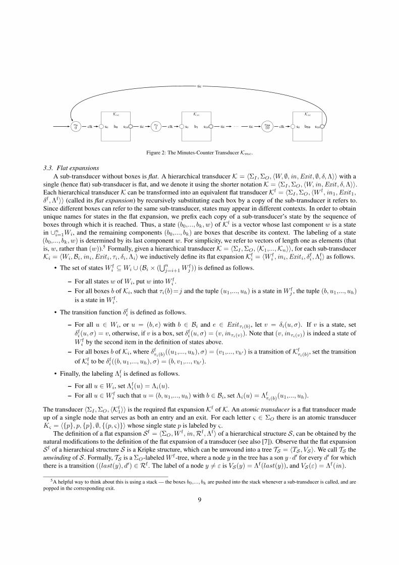
The minutes-counter transducer Kmc, given in Figure 2 is a hierarchical transducer containing 60 states and 60boxes b0,..., b59, all referring to the same subtransducer Ksc, which is the seconds-counter from Figure 1 with thestate s59 serving as an exit with respect to the tic signal 4. Thus, the transition inside Ksc whose source is state s59

and is labeled by tic is removed. This is done because we need to connect one structure to the following one withoutintroducing nondeterminism. The updating of the minutes’ display is handled by 60 states numbered from m0 (whichis also the initial state of the transducer) to m59, each of which is labeled by a set of output signals ΣO = 0,..., 59encoding the number of passed minutes. When the computation is in the state s59 of a box bi and it receives a tic signal,it exits the box and enters the state mi+1, which increments the minutes display. At the next system clock signal clkthe computation enters box bi+1 that resets the seconds display and starts counting the 59 seconds. Note that, by ourassumptions on the hardware, we can safely assume that while in state mi+1 there is no need to process tic and stssignals. However, for completeness, one can assume they are handled by a self loop (which we do not draw).

It is not hard to see how one can use the minutes-counter transducer as a sub-transducer of a more elaboratechronograph capable of counting up to 24 hours, and then use that as a sub-transducer for a chronograph that alsocounts days, etc.

3A natural way to build a chronograph using flip-flops and combinatorial logic is to have one counter counting from 0 to 59 seconds using aclock that ticks once a second, and another counter that counts from 0 to 59 minutes using as its clock the carry (or overflow) flag of the first counter.Thus, the input signals to the minutes counter are derived from the output signals of the seconds counter. Unfortunately, this kind of synthesis (calleddata flow synthesis) is known to be undecidable already for the very restricted case of LTL specifications and systems that are merely pipelines [39].

4The synthesis algorithm we present in this article automatically takes care of designating certain states as exits when it makes use of a librarytransducer with no exits (like the seconds-counter) while constructing another transducer (like the minutes-counter). Note that for this example weuse a definition of hierarchical transducers that allows states to maintain their internal transitions on some input signals, and act as exits only withrespect to the remaining signals.

8

m0

0

Ksc

s0 s59b0m1

1

Ksc

s0 s59b1 · · · m59

59

Ksc

s0 s59b59clk tic clk tic tic clk

tic

Figure 2: The Minutes-Counter Transducer Kmc.

3.3. Flat expansionsA sub-transducer without boxes is flat. A hierarchical transducer K = 〈ΣI ,ΣO, 〈W, ∅, in,Exit , ∅, δ,Λ〉〉 with a

single (hence flat) sub-transducer is flat, and we denote it using the shorter notation K = 〈ΣI ,ΣO, 〈W, in,Exit , δ,Λ〉〉.Each hierarchical transducer K can be transformed into an equivalent flat transducer Kf = 〈ΣI ,ΣO, 〈W f , in1,Exit1,δf ,Λf〉〉 (called its flat expansion) by recursively substituting each box by a copy of the sub-transducer it refers to.Since different boxes can refer to the same sub-transducer, states may appear in different contexts. In order to obtainunique names for states in the flat expansion, we prefix each copy of a sub-transducer’s state by the sequence ofboxes through which it is reached. Thus, a state (b0,..., bk, w) of Kf is a vector whose last component w is a statein ∪ni=1Wi, and the remaining components (b0,..., bk) are boxes that describe its context. The labeling of a state(b0,..., bk, w) is determined by its last component w. For simplicity, we refer to vectors of length one as elements (thatis, w, rather than (w)).5 Formally, given a hierarchical transducer K = 〈ΣI ,ΣO, 〈K1,...,Kn〉〉, for each sub-transducerKi = 〈Wi,Bi, ini,Exit i, τi, δi,Λi〉 we inductively define its flat expansion Kf

i = 〈W fi , ini,Exit i, δ

fi ,Λ

fi〉 as follows.

• The set of states W fi ⊆Wi ∪ (Bi × (

⋃nj=i+1W

fj )) is defined as follows.

– For all states w of Wi, put w into W fi .

– For all boxes b of Ki, such that τi(b)=j and the tuple (u1,..., uh) is a state in W fj , the tuple (b, u1,..., uh)

is a state in W fi .

• The transition function δfi is defined as follows.

– For all u ∈ Wi, or u = (b, e) with b ∈ Bi and e ∈ Exitτi(b), let v = δi(u, σ). If v is a state, setδfi(u, σ) = v, otherwise, if v is a box, set δf

i(u, σ) = (v, inτi(v)). Note that (v, inτi(v)) is indeed a state ofW fi by the second item in the definition of states above.

– For all boxes b of Ki, where δfτi(b)

((u1,..., uh), σ) = (v1,..., vh′) is a transition of Kfτi(b)

, set the transitionof Kf

i to be δfi((b, u1,..., uh), σ) = (b, v1,..., vh′).

• Finally, the labeling Λfi is defined as follows.

– For all u ∈Wi, set Λfi(u) = Λi(u).

– For all u ∈W fi such that u = (b, u1,..., uh) with b ∈ Bi, set Λi(u) = Λf

τi(b)(u1,..., uh).

The transducer 〈ΣI ,ΣO, 〈Kf1〉〉 is the required flat expansion Kf of K. An atomic transducer is a flat transducer made

up of a single node that serves as both an entry and an exit. For each letter ς ∈ ΣO there is an atomic transducerKς = 〈p, p, p, ∅, (p, ς)〉 whose single state p is labeled by ς .

The definition of a flat expansion S f = 〈ΣO,W f , in,Rf ,Λf〉 of a hierarchical structure S , can be obtained by thenatural modifications to the definition of the flat expansion of a transducer (see also [7]). Observe that the flat expansionS f of a hierarchical structure S is a Kripke structure, which can be unwound into a tree TS = 〈TS , VS〉. We call TS theunwinding of S . Formally, TS is a ΣO-labeled W f -tree, where a node y in the tree has a son y ·d′ for every d′ for whichthere is a transition ((last(y), d′) ∈ Rf . The label of a node y 6= ε is VS(y) = Λf(last(y)), and VS(ε) = Λf(in).

5A helpful way to think about this is using a stack — the boxes b0,..., bk are pushed into the stack whenever a sub-transducer is called, and arepopped in the corresponding exit.

9

3.4. Run of a transducer

Consider a hierarchical transducer K with Exit1 = ∅ that interacts with its environment. At point j in time, theenvironment provides K with an input σj ∈ ΣI , and in response K moves to a new state, according to its transitionrelation, and outputs the label of that state. The result of this infinite interaction is a computation of K, called thetrace of the run of K on the word σ1 · σ2 · · · . In the case that Exit1 6= ∅, the interaction comes to a halt wheneverK reaches an exit e ∈ Exit1, since top-level exits have no outgoing transitions. Formally, a run of a hierarchicaltransducer K is defined by means of its flat expansion Kf . Given a finite input word v = σ1 · · ·σm ∈ Σ∗I , a run(computation) of K on v is a sequence of states r = r0 · · · rm ∈ (W f)∗ such that r0 = in1, and rj = δf(rj−1, σj),for all 0 < j ≤ m. Note that since K is deterministic it has at most one run on every word, and that if Exit1 6= ∅then K may not have a run on some words. The trace of the run of K on v is the word of inputs and outputstrc(K, v) = (Λf(r1), σ1) · · · (Λf(rm), σm) ∈ (ΣO × ΣI)

∗. The notions of traces and runs are extended to infinitewords in the natural way.

The computations of K can be described by a computation tree whose branches correspond to the runs of K onall possible inputs, and whose labeling gives the traces of these runs. Note that the root of the tree corresponds to theempty word ε, and its labeling is not part of any trace. However, if we look at the computation tree of K as a sub-tree ofa computation tree of a transducer K′ of which K is a sub-transducer, then the labeling of the root of the computationtree of K is meaningful, and it corresponds to the last element in the trace of the run of K′ leading to the initial stateof K. Formally, given σ ∈ ΣI , the computation tree TK,σ = 〈TK,σ, VK,σ〉, is a (ΣO × ΣI)-labeled (W f × ΣI)-tree,where: (i) the root ε is labeled by (Λf(in1), σ); (ii) a node y = (r1, σ1) · · · (rm, σm) ∈ (W f × ΣI)

+ is in TK,σ iffin1 · r1 · · · rm is the run of K on v = σ1 · · ·σm, and its label is VK,σ(y) = (Λf(rm), σm). Thus, for a node y, thelabels of the nodes on the path from the root (excluding the root) to y are exactly trc(K, v). Observe that the leaves ofTK,σ correspond to pairs (e, σ′), where e ∈ Exit1 and σ′ ∈ ΣI . However, if Exit1 = ∅, then the tree has no leaves,and it represents the runs of K over all words in Σ∗I . We sometimes consider a leaner computation tree TK = 〈TK, VK〉that is a ΣO-labeled ΣI -tree, where a node y ∈ Σ+

I is in TK iff there is a run r of K on y. The label of such a node isVK(y) = Λf(last(r))) and the label of the root is Λf(in1). Observe that for every σ ∈ ΣI , the tree TK can be obtainedfrom TK,σ by simply deleting the first component of the directions of TK,σ , and the second component of the labels ofTK,σ .

Recall that the labeling of the root of a computation tree of K is not part of any trace (when it is not a sub-tree ofanother tree). Hence, in the definition below, we arbitrarily fix some letter % ∈ ΣI . Given a temporal logic formula ϕ,over the atomic propositions AP where 2AP = ΣO × ΣI , we have the following:

Definition 3.1. A hierarchical transducer K = 〈ΣI ,ΣO, 〈K1,...,Kn〉〉, with Exit1 = ∅, satisfies a formula ϕ (writtenK |= ϕ) iff the tree TK,% satisfies ϕ, for an arbitrary fixed letter % ∈ ΣI .

Observe that given ϕ, finding a flat transducer K such that K |= ϕ is the classic synthesis problem studied (for LTLformulas) in [47].

4. Hierarchical Synthesis

In this section we describe our algorithm for bottom-up synthesis of a hierarchical transducer from a libraryof hierarchical transducers. For our purpose, a library L is simply a finite set of hierarchical transducers with thesame input and output alphabets. Formally, L = K1,...,Kλ, and for every 1 ≤ i ≤ λ, we have that Ki =〈ΣI ,ΣO, 〈Ki1,...,Kini

〉〉. Note that a transducer in the library can be a sub-transducer of another one, or share commonsub-transducers with it. The set of transducers in L that have no top-level exits is denoted by L=∅ = Ki ∈ L :Exit i1 = ∅, and its complement is L6=∅ = L \ L=∅.

The synthesis algorithm is provided with an initial library L0 of hierarchical transducers. A good starting point isto include in L0 all the atomic transducers, as well as any other relevant hierarchical transducers, for example from astandard library. Obviously, the choice of the initial library is entirely in the hands of the designer. We then proceed bysynthesizing in rounds. At each round i > 0, the system designer provides a specification formula ϕi of the currentlydesired hierarchical transducer Ki, which is then automatically synthesized using the transducers in Li−1 as possiblesub-transducers. Once a new transducer is synthesized it is added to the library, to be used in subsequent rounds.Technically, the hierarchical transducer synthesized in the last round is the output of the algorithm.

10

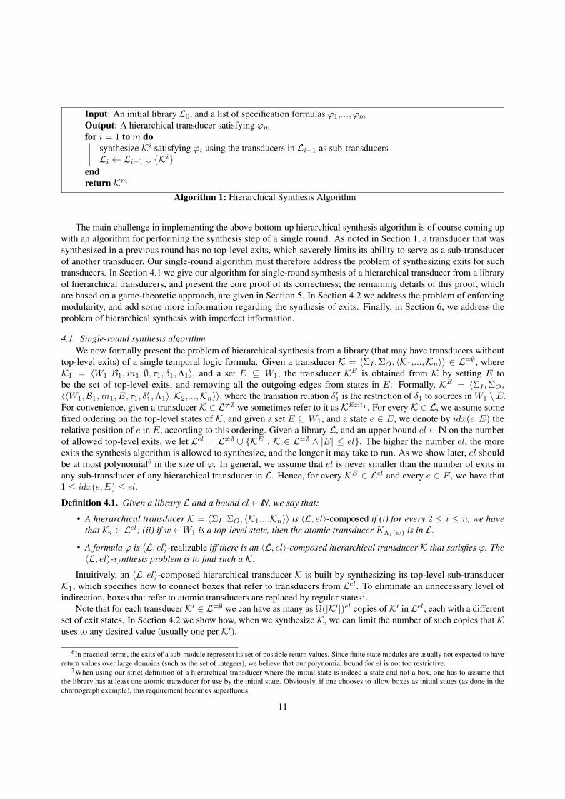
Input: An initial library L0, and a list of specification formulas ϕ1,..., ϕmOutput: A hierarchical transducer satisfying ϕmfor i = 1 to m do

synthesize Ki satisfying ϕi using the transducers in Li−1 as sub-transducersLi ← Li−1 ∪ Ki

endreturn Km

Algorithm 1: Hierarchical Synthesis Algorithm

The main challenge in implementing the above bottom-up hierarchical synthesis algorithm is of course coming upwith an algorithm for performing the synthesis step of a single round. As noted in Section 1, a transducer that wassynthesized in a previous round has no top-level exits, which severely limits its ability to serve as a sub-transducerof another transducer. Our single-round algorithm must therefore address the problem of synthesizing exits for suchtransducers. In Section 4.1 we give our algorithm for single-round synthesis of a hierarchical transducer from a libraryof hierarchical transducers, and present the core proof of its correctness; the remaining details of this proof, whichare based on a game-theoretic approach, are given in Section 5. In Section 4.2 we address the problem of enforcingmodularity, and add some more information regarding the synthesis of exits. Finally, in Section 6, we address theproblem of hierarchical synthesis with imperfect information.

4.1. Single-round synthesis algorithmWe now formally present the problem of hierarchical synthesis from a library (that may have transducers without

top-level exits) of a single temporal logic formula. Given a transducer K = 〈ΣI ,ΣO, 〈K1,...,Kn〉〉 ∈ L=∅, whereK1 = 〈W1,B1, in1, ∅, τ1, δ1,Λ1〉, and a set E ⊆ W1, the transducer KE is obtained from K by setting E tobe the set of top-level exits, and removing all the outgoing edges from states in E. Formally, KE = 〈ΣI ,ΣO,〈〈W1,B1, in1, E, τ1, δ

′1,Λ1〉,K2,...,Kn〉〉, where the transition relation δ′1 is the restriction of δ1 to sources in W1 \E.

For convenience, given a transducer K ∈ L 6=∅ we sometimes refer to it as KExit1 . For every K ∈ L, we assume somefixed ordering on the top-level states of K, and given a set E ⊆ W1, and a state e ∈ E, we denote by idx(e, E) therelative position of e in E, according to this ordering. Given a library L, and an upper bound el ∈ IN on the numberof allowed top-level exits, we let Lel = L 6=∅ ∪ KE : K ∈ L=∅ ∧ |E| ≤ el. The higher the number el, the moreexits the synthesis algorithm is allowed to synthesize, and the longer it may take to run. As we show later, el shouldbe at most polynomial6 in the size of ϕ. In general, we assume that el is never smaller than the number of exits inany sub-transducer of any hierarchical transducer in L. Hence, for every KE ∈ Lel and every e ∈ E, we have that1 ≤ idx(e, E) ≤ el.Definition 4.1. Given a library L and a bound el ∈ IN, we say that:

• A hierarchical transducer K = 〈ΣI ,ΣO, 〈K1,...Kn〉〉 is 〈L, el〉-composed if (i) for every 2 ≤ i ≤ n, we havethat Ki ∈ Lel; (ii) if w ∈W1 is a top-level state, then the atomic transducer KΛ1(w) is in L.

• A formula ϕ is 〈L, el〉-realizable iff there is an 〈L, el〉-composed hierarchical transducer K that satisfies ϕ. The〈L, el〉-synthesis problem is to find such a K.

Intuitively, an 〈L, el〉-composed hierarchical transducer K is built by synthesizing its top-level sub-transducerK1, which specifies how to connect boxes that refer to transducers from Lel. To eliminate an unnecessary level ofindirection, boxes that refer to atomic transducers are replaced by regular states7.

Note that for each transducer K′ ∈ L=∅ we can have as many as Ω(|K′|)el copies of K′ in Lel, each with a differentset of exit states. In Section 4.2 we show how, when we synthesize K, we can limit the number of such copies that Kuses to any desired value (usually one per K′).

6In practical terms, the exits of a sub-module represent its set of possible return values. Since finite state modules are usually not expected to havereturn values over large domains (such as the set of integers), we believe that our polynomial bound for el is not too restrictive.

7When using our strict definition of a hierarchical transducer where the initial state is indeed a state and not a box, one has to assume thatthe library has at least one atomic transducer for use by the initial state. Obviously, if one chooses to allow boxes as initial states (as done in thechronograph example), this requirement becomes superfluous.

11

4.1.1. Connectivity treesIn the classical automata-theoretic approach to synthesis [47], synthesizing a system is reduced to the problem

of finding a regular tree that is a witness to the non-emptiness of a tree automaton running on computation trees.At first glance, it looks like extending this approach to solve our hierarchical synthesis problem may not be toohard: if we can build an automaton that only accepts a computation tree if it corresponds to an 〈L, el〉-composedhierarchical transducer then, by taking the product of this automaton with an automaton that only accepts models of thespecification formula, our synthesis problem reduces to finding a (regular) witness to the non-emptiness of the productautomaton. Unfortunately, this natural extension fails since it is impossible to construct an automaton that can detect ifthe computation tree specifies the moves from exits of one transducer to the entry of another transducer in a consistentway. The difficulty is that the destination to move to from an exit depends only on the exit and the next input letter,and is independent of how that exit was reached (inside the current transducer). Thus, all paths in the computationtree that reach the same exit of the current transducer must agree on the next transducer to move to (on the same inputletter). Observe that such paths may have nodes that are arbitrarily far apart since they correspond to moves of thetransducer on different input words. Indeed, it is not hard to come up with an example where two disjoint infinite pathsmust agree on infinitely many moves from exits to entrances. This infinite amount of synchronization provides verystrong evidence that trying to solve the problem by adding extra annotations to the computation tree, and/or by havingcopies of the automaton that read different paths coordinate by carrying with them identical guesses, would also fail.

We thus solve the (single-round) hierarchical synthesis problem by reducing it to the non-emptiness problem of atree automaton whose input is not a computation tree, but rather a system description in the form of a connectivitytree (inspired by the “control-flow” trees of [39]), which describes how to connect library components in a way thatsatisfies the specification formula. Specifically, given a library L = K1,...,Kλ and a bound el ∈ IN, connectivitytrees represent hierarchical transducers that are 〈L, el〉-composed, in the sense that every 〈L, el〉-composed hierarchicaltransducer induces a regular connectivity tree, and vice versa.

Formally, a connectivity tree T = 〈T, V 〉 for L and el, is an Lel-labeled complete (1,..., el × ΣI)-tree, wherethe root is labeled by an atomic transducer. Intuitively, a node x with V (x) = KE represents a top-level state qif KE is an atomic transducer, and otherwise it represents a top-level box b that refers to KE . The label of a sonx · (idx(e, E), σ) specifies the destination of the transition from the exit e of b (or from a state q, if KE is atomic— in which case it has a single exit) when reading σ. Sons x · (i, σ), for which i > |E|, are ignored. Thus, a pathπ = (i0, σ0) · (i1, σ1) · · · in a connectivity tree T is called meaningful, iff for every j > 0, we have that ij is notlarger than the number of top-level exits of V (ij−1, σj−1). A connectivity tree T = 〈T, V 〉 is regular if there is a flattransducerM = 〈1,..., el × ΣI ,Lel, 〈M,m0, ∅, δT,ΛT 〉〉, such that T is equal to the (lean) computation tree TM.

Lemma 4.1. Every 〈L, el〉-composed hierarchical transducer induces a regular connectivity tree, and every regularconnectivity tree for L and el induces an 〈L, el〉-composed hierarchical transducer.

Proof. For the first direction, let K = 〈ΣI ,ΣO, 〈K1,...,Kn〉〉, where K1 = 〈W1,B1, in1, τ1, δ1,Λ1〉, be an 〈L, el〉-composed hierarchical transducer. We construct a flat transducer M whose computation tree TM is the requiredconnectivity tree. The elements ofM are as follows:

• M = W1 ∪ B1, and m0 = in1.

• If w ∈ W1, then for every σ ∈ ΣI , we have that δT (w, (1, σ)) = δ1(w, σ), and for every 1 < i ≤ el we(arbitrarily) let δT (w, (i, σ)) = m0.

• For b ∈ B1, let KE ∈ Lel be the sub-transducer that b refers to. For every σ ∈ ΣI , if 1 ≤ i ≤ |E| thenδT (b, (i, σ)) = δ1((b, e), σ), where e ∈ E is such that idx(e, E) = i; and if |E| < i ≤ el then we (arbitrarily)let δT (b, (i, σ)) = m0.

• For w ∈W1 we have that ΛT (w) = Kς , where Λ1(w) = ς .

• For b ∈ B1 we have that ΛT (b) = Kτ1(b).

Recall that a son y · (i, σ), of a node y in a connectivity tree T = 〈T, V 〉, is meaningless if i is larger than the numberof exits of the transducer V (y). Hence, our choice to direct the corresponding transitions of M to the node m0 isarbitrary and was done only for technical completeness.

12

For the other direction, given a regular connectivity tree T = 〈T, V 〉 generated by the transducerM = 〈1,..., el× ΣI ,Lel, 〈M,m0, ∅, δT,ΛT 〉〉, it is not hard to see that it induces an 〈L, el〉-composed hierarchical transducer K,whose top-level sub-transducer K1 is basically a replica ofM. Every node m ∈M becomes a state of K1 if ΛT (m) isan atomic transducer and, otherwise, it becomes a box of K1 which refers to the top-level sub-transducer of ΛT (m).The destination of a transition from an exit e of a box m, with ΛT (m) = KE , when reading a letter σ ∈ ΣI , isgiven by δT (m, (idx(e, E), σ)). If m is a state, then ΛT (m) is an atomic transducer with a single exit and thus,the destination of a transition from m when reading a letter σ ∈ ΣI , is given by δT (m, (1, σ)). For a box b of K1,let ΛT (b) = 〈ΣI ,ΣO, 〈K(b,1),...K(b,nb)〉〉, and denote by sub(b) = K(b,1),...K(b,nb) the set of sub-transducers ofΛT (b), and by E(b) the set of top-level exits of ΛT (b).

Formally, K = 〈ΣI ,ΣO, 〈K1,...,Kn〉〉, where K1 = 〈W1,B1,m0, τ1, δ1,Λ1〉, and:

• W1 = w ∈ M : ∃ς ∈ ΣO s.t. ΛT (w) = Kς. Note that since the root of a connectivity tree is labeled by anatomic transducer then m0 ∈W1.

• B1 = M \W1.

• The sub-transducers K2,...,Kn =⋃b∈B1 sub(b).

• For b ∈ B1, we have that τ1(b) = i, where i is such that Ki = K(b,1).

• For w ∈W1, and σ ∈ ΣI , we have that δ1(w, σ) = δT (w, (1, σ)).

• For b ∈ B1, we have that δ1((b, e), σ) = δT (b, (idx(e, E(b)), σ)), for every e ∈ E(b) and σ ∈ ΣI .

• Finally, for w ∈W1 we have that Λ1(w) = ς , where ς is such that ΛT (w) = Kς .

We now come back to the chronograph example and give a description of the connectivity tree of an extra component,the counter of hours, which is synthesized from the already described hierarchical minutes-counter transducer.

Example 4.1 (Hours-Counter Transducer). Suppose we want to synthesize an hours-counter from a library of simplertransducers, such as the minutes-counter and some atomic transducers (to be used as internal states of the desiredmachine). For instance, we can consider the following library L = Kmc,K0,...,K23, where Kms is the minutes-counter transducer presented in Example 3.1 and K0,...,K23 represent 24 “states” for the output of hour signals(for the display module) from 0 to 23, respectively. Since Kmc can have as an exit the last state of its internal boxb59, the synthesis algorithm can succeed already with the bound el on the number of exits set to 1, using KEmc ∈ L1,where E = b59.s59 with respect to the tic signal8. Now, once a reasonable specification of the right behavior ofthe hours-counter is given by a temporal logic formula, we can run our synthesis algorithm on L1, from which wemay derive, as a possible outcome, the hierarchical transducer Khc depicted in Part (a) of Figure 3. Observe thatall atomic transducers are depicted as classic internal states. The hours-counter transducer Khc has a structure thatis very similar to that of the minutes-counter Kmc. It is a hierarchical machine having 24 boxes, from b0 to b23, allreferring to the same subtransducer KEmc, plus 24 states. Each box bi describes the elapsing of minutes within the(i + 1)-th hour. Note that, as we did with the minutes-counter, we can safely assume that the states K0,...,K23 donot have to process tic and sts signals. For the sake of completness, one can assume self loops (which we do notdraw in the figure) on these states for these signals. Part (b) of Figure 3 shows one path of the computation tree of thehours-counter transducer (for readability, we do not show the whole tree). Each node in this path is written by givingthe labelling of the node, and above it the last letter of the node’s name (i.e., an input signal together with the numberof the exit — which is always 1 since el = 1). For example, the root of the tree, representing the first component K0

in the hierarchical transducer Khc, has ε as its name (since at the beginning there is no input) and its labelling isK0. This node has a son, called (1, clk), which represents the move from K0 when a clk signal is received. The node(1, clk) is labelled by KEmc since it represents the box b0. The edge from the node (1, clk) to the son (1, clk) · (1, tic),which is labelled by K1, implies that when a computation reaches the exit b59.s59 of KEmc and a tic signal is received,the computation moves to the state K1.

8Note that, like in the previous example, we consider a setting where boxes may also serve as exits, and only with respect to some signals.

13

K00

KEmc

m0 b59.s59b0K11

KEmc

m0 b59.s59b1 · · · K2323

KEmc

m0 b59.s59b23clk tic clk tic tic clk

tic

(a) The counter.

εK0

(1,clk)

KEmc

(1,tic)

K1

(1,clk)

KEmc

· · ·

(b) Part of the connectivity tree.

Figure 3: The Hours-Counter Transducer Khc and its connectivity tree.

4.1.2. From synthesis to automata emptinessGiven a library L = K1,...,Kλ, a bound el ∈ IN, and a temporal logic formula ϕ, our aim is to build an APT

ATϕ such that it accepts a regular connectivity tree T = 〈T, V 〉 iff it induces a hierarchical transducer K such thatK |= ϕ. Recall that by Definition 3.1 and Theorem 2.1, K |= ϕ iff TK,% is accepted by the SAPT Aϕ. The basic idea isthus to have ATϕ simulate all possible runs of Aϕ on TK,%. Unfortunately, since ATϕ has as its input not TK,%, but theconnectivity tree T , this is not a trivial task. In order to see how we can solve this problem, we first have to make thefollowing observation.

Let T = 〈T, V 〉 be a regular connectivity tree, and let K be the hierarchical transducer that it induces. Considera node u in the computation tree TK,% which corresponds to a point along a computation where K just enters a toplevel box b (or state9). That is, last(u) = ((b, inτ1(b)), σ). Observe that the root of TK,% is such a node. Let KEbe the library sub-transducer that b refers to, and note that the sub-tree T u, rooted at u, represents the traces ofcomputations of K that start from the initial state of KE , in the context of the box b. The sub-tree prune(T u), obtainedby pruning every path in T u at the first node u, with last(u) = ((b, e), σ) for some e ∈ E and σ ∈ ΣI (i.e., at the firstpoint the computation reaches an exit of KE), represents the portions of these traces that stay inside KE . Note thatprune(T u) is essentially independent of the context b in which KE appears, and is isomorphic to the computationtree TKE ,σ of KE (the isomorphism being to simply drop the component b from every letter in the name of everynode in prune(T u)). Moreover, every son v (in TK,%), of such a leaf u of prune(T u), is of the same form as u. I.e.,last(v) = ((b′, inτ1(b′)), σ

′), where b′ = δ1((b, e), σ′) is a top-level box (or state) of K. Indeed, once an exit of atransducer referred to by a top level box of K is reached, a computation of K must proceed, according to the transitionrelation δ1 of it’s top level sub-transducer K1, either to a top level state or to the entrance of another top level box. Itfollows that TK,% is isomorphic to a concatenation of sub-trees of the form TKE ,σ, where the transition from a leaf ofone such sub-tree to the root of another is specified by the transition relation δ1, and is thus given explicitly by theconnectivity tree T .

The last observation is the key to how ATϕ can simulate, while reading T , all the possible runs of Aϕ on TK,%.The general idea is as follows. Consider a node u of TK,% such that prune(T u) is isomorphic to TKE ,σ. A copy ofATϕ that reads a node y of T labeled by KE can easily simulate, without consuming any input, all the portions ofthe runs of any copy of Aϕ that start by reading u and remain inside prune(T u). This simulation can be done bysimply constructing TKE ,σ on the fly and running Aϕ on it. For every simulated copy of Aϕ that reaches a leaf u ofprune(T u), the automaton ATϕ sends copies of itself to the sons of y in the connectivity tree in order to continue thesimulation of Aϕ on the different sub-trees of TK,% rooted at sons of u. Recall that last(u) is of the form ((b, e), σ),that is, u represents a point in a computation of K where an exit e of a top level box b is reached. Observe that for everyinput letter σ′ ∈ ΣI , the node z = y · (idx(e, E), σ′) in the connectivity tree represents the box b′ to which K shouldproceed from exit e of box b when reading σ′, and the label of z is the library sub-transducer to which b′ refers. Thus,the simulation of a copy of Aϕ that proceeds to a son v = u · ((b′, inτ1(b′)), σ

′) is handled by a copy of ATϕ that is sent

9Here we think of top-level states of K as boxes that refer to atomic transducers.

14

to the son z = y · (idx(e, E), σ′).Our construction of ATϕ implements the above idea, with one important modification. In order to obtain optimal

complexity in successive rounds of Algorithm 1, it is important to keep the size of ATϕ independent of the size of thetransducers in the library. Unfortunately, simulating the runs of Aϕ on TKE ,σ on the fly would require an embedding ofKE inside ATϕ . Recall, however, that no input is consumed by ATϕ while running such a simulation. Hence, we canperform these simulations off-line instead, in the process of building the transition relation of ATϕ . Obviously, thisrequires a way of summarizing the possibly infinite number of runs of Aϕ on TKE ,σ, which we do by employing theconcept of summary functions from [8]. Let Aϕ = 〈ΣO × ΣI , Qϕ, q

0ϕ, δϕ, Fϕ〉, let Aqϕ be the automaton Aϕ using

q ∈ Q as an initial state, and let C be the set of colors used in the acceptance condition Fϕ. Following the aboveobservations, we next turn our attention to the problem of how to effectively summarize the run 〈Tr, r〉 of Aqϕ onTKE ,σ .

First, we define a total ordering on the set of colors C by letting c c′ when c is better, from the point of viewof the parity acceptance condition of Aϕ, than c′. Thus, any even color is better than all the odd colors, the larger theeven color the better, and if one has to choose between two odd colors it is best to “minimize the damage” by taking thesmaller odd number. Formally, c c′ if the following holds: if c′ is even then c is even and c ≥ c′; and if c′ is odd theneither c is even, or c is also odd and c ≤ c′. For example: 4 2 0 1 3. We denote by min the operation oftaking the minimal color, according to , of a finite set of colors.

Consider now the run tree 〈Tr, r〉 ofAqϕ on TKE ,σ . Note that if z ∈ Tr is a leaf, then r(z) is of the form (a·(e, σ′), p)for some string a, with p ∈ Q∨,∧ϕ (i.e., p is not an ε-state), and e ∈ E. Indeed, if p is an ε-state then Aqϕ can proceedwithout consuming any input, and hence the run can be extended beyond z; similarly, if e is not an exit of KE thenit has successors inside KE , and again the run can be extended beyond z. Every such leaf z represents a copy ofAϕ that is in state p and is reading a node of the computation tree of KE whose last component is (e, σ′). It turnsout (and is proved in [8]) that it is not important to remember all the colors this copy of Aϕ encountered along theway to this node, but only the maximal color according to (this ultimately hinges upon the fact that parity gamesare memoryless – see [8]). It is also not important to differentiate between two copies of Aϕ that have reached twodifferent nodes y, y′ of the computation tree of KE if last(y) = last(y′) = (e, σ′) (thus both copies are going to readthe same future input sub-tree) and both copies are in the same state p and have encountered the same maximal color.Moreover, if there are two copies of Aϕ that have reached, with the same state p, two (possibly the same) nodes y, y′

with last(y) = last(y′) = (e, σ′), but have encountered different maximal colors c, c′ where c c′, it is enough toremember the information of the copy that is “more behind” in its attempt to satisfy the acceptance condition. I.e., thecopy that encountered c′. The intuitive reason is that since both copies are going to read the same input sub-tree fromthe same state, if the copy that has encountered a less favorable maximal color in the past is going to accept then thecopy that encountered a more favorable color is bound to accept too.

To capture the above intuition, we define a function gr : E ×ΣI ×Q∨,∧ϕ → C ∪ a, called the summary functionof 〈Tr, r〉, which summarizes this run. Given h = (e, σ′, p) ∈ E × ΣI ×Q∨,∧ϕ , if there is no leaf z ∈ Tr, such thatr(z) is of the form (a · (e, σ′), p), then gr(h) =a; otherwise, gr(h) = c, where c is the maximal color encounteredby the copy of Aϕ which made the least progress towards satisfying the acceptance condition, among all copies thatreach a leaf z ∈ Tr of the form (a · (e, σ′), p). Formally, given h = (e, σ′, p) ∈ E × ΣI ×Q∨,∧ϕ , let paths(r, h) bethe set of all the paths in 〈Tr, r〉 that end in a leaf z ∈ Tr with r(z) = (a · (e, σ′), p), for some a. Then, gr(h) =a ifpaths(r, h) = ∅ and otherwise, gr(h) = minmaxC(π) : π ∈ paths(r, h).

Let Sf (KE , σ, q) be the set of summary functions of the runs of Aqϕ on TKE ,σ. If TKE ,σ has no leaves, thenSf (KE , σ, q) contains only the empty summary function ∅. For g ∈ Sf (KE , σ, q), let g 6=a = h ∈ E × ΣI ×Q∨,∧ϕ :

g(h) 6=a. Based on the ordering we defined for colors, we can define a partial order on Sf (KE , σ, q), by lettingg g′ if for every h ∈ (E × ΣI × Q∨,∧ϕ ) the following holds: g(h) =a, or g(h) 6=a6= g′(h) and g(h) g′(h).Observe that if r and r′ are two non-rejecting runs, and gr gr′ , then extending r to an accepting run on a tree thatextends TKE ,σ is always not harder than extending r′ - either because Aϕ has less copies at the leaves of r, or becausethese copies encountered better maximal colors. Given a summary function g, we say that a run 〈Tr, r〉 achieves gif gr g; we say that g is feasible if there is a run 〈Tr, r〉 that achieves it; and we say that g is relevant if it can beachieved by a memoryless10 run that is not rejecting (i.e., by a run that has no infinite path that does not satisfy the

10A run of an automatonA is memoryless if two copies ofA that are in the same state, and read the same input node, behave in the same way on

15

acceptance condition of Aϕ). We denote by Rel(KE , σ, q) ⊆ Sf (KE , σ, q) the set of relevant summary functions.We are now ready to give a formal definition of the automaton ATϕ . Given a library L = K1,...,Kλ, a bound

el ∈ IN, and a temporal-logic formula ϕ, letAϕ = 〈ΣO×ΣI , Qϕ, q0ϕ, δϕ, Fϕ〉, let C = Cmin,..., Cmax be the colors

in the acceptance condition of Aϕ, and for KE ∈ Lel, let ΛE be the labeling function of the top-level sub-transducer ofKE . The automaton ATϕ = 〈Lel, (1,..., el × ΣI), (ΣI ×Q∨,∧ϕ × C) ∪ q0, q0, δ, α〉 has the following elements.

• For every KE ∈ Lel we have that δ(q0,KE) = δ((%, q0ϕ, Cmin),KE) if KE is an atomic transducer and,

otherwise, δ(q0,KE) = false.

• For every (σ, q, c) ∈ ΣI × Q∨,∧ϕ × C, and every KE ∈ Lel, we have δ((σ, q, c),KE) =∨g∈Rel(KE,σ,q)∧

(e,σ,q)∈g 6=a⊕σ′∈ΣI

((idx(e, E), σ′), (σ′, δϕ(q, (ΛE(e), σ)), g(e, σ, q))), where⊕

=∧

if q ∈ Q∧ϕ, and⊕

=∨if q ∈ Q∨ϕ.

• α(q0) = Cmin; and α((σ, q, c)) = c, for every (σ, q, c) ∈ ΣI ×Q∨,∧ϕ × C.

Intuitively, ATϕ first checks that the root of its input tree T is labeled by an atomic proposition and then proceedsto simulate all the runs of Aϕ on TK,%. A copy of ATϕ at a state (σ, q, c), that reads a node y of T labeled by KE ,considers all the non-rejecting runs of Aqϕ on TKE ,σ, by looking at the set Rel(KE , σ, q) of summary functions forthese runs. It then sends copies of ATϕ to the sons of y to continue the simulation of copies of Aϕ that reach the leavesof TKE ,σ .

The logic behind the definition of δ((σ, q, c),KE) is as follows. Since every summary function g ∈ Rel(KE , σ, q)summarizes at least one non-rejecting run, and it is enough that one such run can be extended to an accepting run ofAϕ on the remainder of TK,%, we have a disjunction on all g ∈ Rel(KE , σ, q). Every (e, σ, q) ∈ g 6=a represents one ormore copies of Aϕ at state q that are reading a leaf u of TKE ,σ with last(u) = (e, σ), and all these copies must accepttheir remainders of TK,%. Hence, we have a conjunction over all (e, σ, q) ∈ g 6=a.

A copy of Aϕ that starts at the root of TKE ,σ may give rise to many copies that reach a leaf u of TKE ,σ withlast(u) = (e, σ), but we only need to consider the copy which made the least progress towards satisfying the acceptancecondition, as captured by g(e, σ, q). To continue the simulation of such a copy on its remainder of TK,%, we send a copyofATϕ to a son y · (idx(e, E), σ′) of y in the connectivity tree, whose label specifies where K should go to from the exite when reading σ′, as follows. Recall that the leaf u corresponds to a node u of TK,% such that last(u) = ((b, e), σ)and b is a top-level box of K that refers to KE . Also recall that every node in TK,% has one son for every letter σ′ ∈ ΣI .Hence, a copy of Aϕ that is at state q and is reading u, sends one copy in state q′ = δϕ(q, (ΛE(e), σ)) to each son of u,if q ∈ Q∧ϕ; and only one such copy, to one of the sons of u, if q ∈ Q∨ϕ. This explains why

⊕is a conjunction in the

first case, and is a disjunction in the second. Finally, a copy of ATϕ that is sent to direction (idx(e, E), σ′) carries withit the color g(e, σ, q). The color assigned to q0 is of course arbitrary.

The construction above implies the following lemma:

Lemma 4.2. ATϕ accepts a regular connectivity tree T = 〈T, V 〉 iff T induces a hierarchical transducer K, such thatTK,% is accepted by Aϕ.

Proof. The core of the proof is game-theoretic. Recall that the game-based approach to model checking a flat system Swith respect to a branching-time temporal logic specification ϕ, reduces the model-checking problem to solving a game(called the membership game of S and Aϕ) obtained by taking the product of S with the alternating tree automatonAϕ [36]. In [8], this approach was extended to hierarchical structures, and it was shown there that given a hierarchicalstructure S and an SAPT A, one can construct a hierarchical membership game GS,A such that Player 0 wins GS,Aiff the tree obtained by unwinding S is accepted by A. In particular, when A accepts exactly all the tree models ofa branching-time formula ϕ, the above holds iff S satisfies ϕ. Furthermore, it is shown in [8] that one can simplifythe hierarchical membership game GS,A, by replacing boxes of the top-level arena with gadgets that are built usingPlayer 0 summary functions, and obtain an equivalent flat game Gs

S,A.Given a regular connectivity tree T = 〈T, V 〉 that induces a hierarchical transducer K, we prove Lemma 4.2 by

showing that the flat membership game GsS,Aϕ

, where S is a hierarchical structure whose unwinding is the computation

the rest of the input.

16

tree TK,%, is equivalent to the flat membership game GKT,ATϕ

, of ATϕ and a Kripke structure KT whose unwinding isT . Thus, Aϕ accepts TK,% iff ATϕ accepts T . The equivalence of these two games follows from the fact that they haveisomorphic arenas and winning conditions. Consequently, our proof of Lemma 4.2 is mainly syntactic in nature, andbasically amounts to constructing the structures S and KT , constructing the game GS,Aϕ

, simplifying it to get GsS,Aϕ

,and constructing the membership game GKT,AT

ϕ. The remaining details can be found in Section 5.

We now state our main theorem.

Theorem 4.1. The 〈L, el〉-synthesis problem is EXPTIME-complete for a µ-calculus formula ϕ, and is 2EXPTIME-complete for an LTL formula (for el that is at most polynomial in |ϕ| for µ-calculus, or at most exponential in |ϕ| forLTL).

Proof. The lower bounds follow from the same bounds for the classical synthesis problem of flat systems [34, 49],and the fact that it is immediately reducible to our problem if L contains all the atomic transducers. For the upperbounds, since an APT accepts some tree iff it accepts some regular tree (andATϕ obviously only accepts trees which areconnectivity trees), by Lemma 4.2 and Theorem 2.1, we get that an LTL or a µ-calculus formula ϕ is 〈L, el〉-realizableiff L(ATϕ ) 6= ∅. Checking the emptiness of ATϕ can be done either directly, or by first translating it to an equivalentNPT A′Tϕ . For reasons that will become apparent in Section 4.2 we choose the latter. Note that the known algorithmsfor checking the emptiness of an NPT are such that if L(ATϕ ) 6= ∅, then one can extract a regular tree in L(ATϕ ) fromthe emptiness checking algorithm [48]. The upper bounds follow from the analysis given below of the time required toconstruct ATϕ and check for its non-emptiness.

By Theorem 2.1, the number of states |Qϕ| and the index k of Aϕ is |Qϕ| = 2O(|ϕ|), k = 2 for LTL, and|Qϕ| = O(|ϕ|), k = O(|ϕ|) for µ-calculus. The most time consuming part in the construction of ATϕ is calculating forevery (KE , σ, q) ∈ (Lel × ΣI ×Qϕ), the set Rel(KE , σ, q). Calculating Rel(KE , σ, q) can be done by checking forevery summary function g ∈ Sf (KE , σ, q) if it is relevant. Our proof of Lemma 4.2 also yields that, by [8], the lattercan be done in time O((|K| · |Qϕ|)k · (k + 1)|E|·|Qϕ|·k). Observe that the set Sf (KE , σ, q) is of size (k + 1)|E|, andthat the number of transducers in Lel is O(λ ·mel), where m is the maximal size of any K ∈ L. It follows that for anLTL (resp. µ-calculus) formula ϕ, the automaton ATϕ can be built in time at most polynomial in the size of the library,exponential in el, and double exponential (resp. exponential) in |ϕ|.

We now analyze the time it takes to check for the non-emptiness ofATϕ . Recall that for every η ∈ (Lel×ΣI ×Qϕ),the set Rel(η) is of size at most (k + 1)el, and thus, the size of the transition relation of ATϕ is polynomial in |L| and|ϕ|, and exponential in el. Checking the emptiness of ATϕ is done by first translating it to an equivalent NPT A′Tϕ . By[42], given an APT with |Q| states and index k, running on Σ-labeledD∗-trees, one can build (in time polynomial in thedescriptions of its input and output automata) an equivalent NPT with (|Q| · k)O(|Q|·k) states, an index O(|Q| · k), anda transition relation of size |Σ| · (|Q| · k)O(|D|·|Q|·k). It is worth noting that this blow-up in the size of the automaton isindependent from the size of the transition relation of ATϕ . By [36, 54], the emptiness of A′Tϕ can be checked in time|Σ| · (|Q| · k)O(|D|·|Q|2·k2) (and if it is not empty, a witness is returned). Recall that |Σ| = |Lel| = O(λ ·mel), and that|D| = el · |ΣI |. By substituting the values calculated above for |Q| and k, the theorem follows.

Note that when using the single-round 〈L, el〉-synthesis algorithm as a sub-routine of the multiple-rounds Algo-rithm 1, it is conceivable that the transducerKi synthesized at iteration i will be exponential (or even double-exponentialfor LTL) in the size of the specification formula ϕi. At this point it is probably best to stop the process, refine thespecifications (i.e., break step i into multiple sub-steps), and try again. However, it is important to note that even if theprocess is continued, andKi is added to the library, the time complexity of the succeeding iterations does not deterioratesince the single-round 〈L, el〉-synthesis algorithm is only polynomial in the maximal size m of any transducer in thelibrary.

4.2. Enforcing modularity

In this section, we address two main issues that may hinder the efforts of our single-round 〈L, el〉-synthesisalgorithm to synthesize a succinct hierarchical transducer K.

The first issue is that of ensuring that, when possible, K indeed makes use of the more complex transducers inthe library (especially transducers synthesized in previous rounds) and does not rely too heavily on the less complex,

17

or atomic, transducers. An obvious and most effective solution to this problem is to simply not have some (or all)of the atomic transducers present in the library. The second issue is making sure that K does not have too manysub-transducers, which can happen if it uses too many copies of the same transducer K′ ∈ L=∅, each with a differentset of exits. We also discuss some other points of interest regarding the synthesis of exits.

We address the above issues by constructing, for each constraint we want to enforce on the synthesized transducerK, an APT A, called the constraint monitor, such that A accepts only connectivity trees that satisfy the constraint.

We then synthesizeK by checking the non-emptiness of the product ofATϕ with all the constraints monitors, insteadof the single ATϕ . Note that a nondeterministic monitor (i.e., an NPT) of exponential size can also be used, withoutadversely affecting the time-complexity, if the product with it is taken after we translate the product of ATϕ and theother (polynomial) APT monitors, to an equivalent NPT.

A simple and effective way to enforce modularity in Algorithm 1 is that once a transducerKi is synthesized in roundi, one incorporates in subsequent rounds a monitor that rejects any connectivity tree containing a node labeled by somekey sub-transducers of Ki. This effectively enforces any transducer synthesized using a formula that refers to atomicpropositions present only in Ki (and its disallowed sub-transducers) to use Ki, and not try to build its functionalityfrom scratch. As to other ways to enforce modularity, the question of whether one system is more modular than another,or how to construct a modular system, has received many, and often widely different, answers. Here we only discusshow certain simple modularity criteria can be easily implemented on top of our algorithm. For example, some peoplewould argue that a function that has more than, say, 10 consecutive lines of code in which no other function is called, isnot modular enough. A monitor that checks that in no path in a connectivity tree there are more than 10 consecutivenodes labeled with an atomic transducer can easily enforce such a criterion. We can even divide the transducers in thelibrary into groups, based on how “high level” they are, and enforce lower counts on lower level groups. Essentially,every modularity criterion that can be checked by a polynomial APT, or an exponential NPT, can be used. Enforcingone context-free property can also be done, albeit with an increase in the time complexity. Other non-regular criteriamay be enforced by directly modifying the non-emptiness checking algorithm instead of by using a monitor, and wereserve this for future work.

As for the issue of synthesized exits, recall that for each transducer K′ ∈ L=∅ we can have as many as Ω(|K′|)elcopies of K′ in Lel, each with a different set of exit states. Obviously, we would not like the synthesized transducer Kto use so many copies as sub-transducers. It is not hard to see that one can, for example, build an NPT of size O(|Lel|)that guesses for every K′ ∈ L=∅ a single set of exits E, and accepts a connectivity tree iff the labels of all the nodes inthe tree agree with the guessed exits. Note that after the end of the current round of synthesis, we may choose to addK′E to the library (in addition, or instead of K′).

Another point to note about the synthesis of exits is that while a transducer K surely satisfies the formula ϕi itwas synthesized for, KE may not. Consider for example a transducer K which is simply a single state, labeled withp, with a self loop. If we remove the loop and turn this state into an exit, it will no longer satisfy ϕi = p ∧Xp orϕi = Gp. Now, depending on one’s point of view, this may be either an advantage (more flexibility) or a disadvantage(loss of original intent). We believe that this is mostly an advantage, however, in case it is considered a disadvantage,a few possible solutions come to mind. First, for example if ϕi = Gp, one may wish for K to remain without exitsand enforce E = ∅. Another option, for example if ϕi = p ∧Xp, is to synthesize in round i a modified formula likeϕ′i = p ∧ ¬exit ∧X(p ∧ exit), with the thought of exits in mind. Yet another option is to add, at iterations after i, amonitor that checks that if KE is the label of a node in the connectivity tree then ϕi is satisfied. The monitor can checkthat ϕi is satisfied inside KE , in which case the monitor is a single state automaton, that only accepts if E is such thatKE |= ϕi (possibly using semantics over truncated paths [25]); alternatively, the monitor can check that ϕi is satisfiedin the currently synthesized connectivity tree, starting from the node labeled by KE , in which case the monitor is basedon ATϕi

.

5. Hierarchical Games and the Proof of Lemma 4.2

We now give the details of the proof of Lemma 4.2 which makes heavy use of hierarchical two-player parity games.We start by providing some necessary definitions and constructs. Additional information regarding these constrructscan be found in [8].

18

5.1. The product of a transducer and a Kripke structure

Given a hierarchical transducer K = 〈ΣI ,ΣO, 〈K1,...,Kn〉〉, whose input alphabet ΣI is the output alphabet ofa Kripke structure S = 〈ΣI ,W, in,R,Λ〉, we can build a hierarchical structure K ⊗ S by taking the product of Kand S. The hierarchical structure K ⊗ S has a sub-structure Ki,q for every 2 ≤ i ≤ n and every state q ∈W , whichis essentially the product of the sub-transducer Ki with S, where the initial state of Ki is paired with the state q ofS. For i = 1, we need only the sub-structure K1,in . The hierarchical order of the sub-structures is consistent withthe one in K. Thus, the sub-structure Ki,q can be referred to by boxes of a sub-structure Kj,p only if i > j. LetKi = 〈Wi,Bi, ini,Exit i, τi, δi,Λi〉, then Ki,q = 〈Wi ×W,Bi ×W, (ini, q),Exit i ×W, τi,q,Ri,q,Λi,q〉 is such that:

• For (b, w) ∈ Bi ×W , we have that τi,q(b, w) = (τi(b), w).

• For (u,w) ∈Wi ×W , we have that ((u,w), (v, w′)) ∈ Ri,q iff (w,w′) ∈ R and δi(u,Λ(w′)) = v.

• For (b, w) ∈ Bi ×W , and an exit (e, w′) ∈ Exitτi(b) ×W of it, we have that 〈((b, w), (e, w′)), (v, w′′)〉 ∈ Ri,qiff (w′, w′′) ∈ R and δi((b, e),Λ(w′′)) = v.

• For (u,w) ∈Wi ×W , we have that Λi,q((u,w)) = (Λi(u),Λ(w)).

Given σ ∈ ΣI , consider the Kripke structure Sσ = 〈ΣI ,ΣI , σ,ΣI × ΣI ,ΣI × ΣI〉, that has one state for everyletter in ΣI (labeled by that letter), its initial state is σ, and it has a transition from every letter to every letter. Then, it iseasy to see that the following holds.

Lemma 5.1. Given a hierarchical transducer K, and a letter σ ∈ ΣI , the computation tree TK,σ can be obtained byunwinding the hierarchical structure K ⊗ Sσ .

5.2. Hierarchical membership games

A hierarchical two-player game [8] is a game played between two players, referred to as Player 0 and Player 1.The game is defined by means of a hierarchical arena and a winning condition. The players move a token along thehierarchical arena, and the winning condition specifies the objectives of the players as to the sequence of states traversedby the token. A hierarchical arena is a hierarchical structure with an empty output alphabet, in which the state space ofeach of the underlying sub-structures is partitioned into states belonging to Player 0 and states belonging to Player 1.When the token is in a state belonging to one of the players, it chooses a successor to which the token is moved. Werefer to the underlying substructures as sub-arenas. Formally, a hierarchical two-player game is a pair G = (V,Γ),where V = 〈V1,...,Vn〉 is a hierarchical arena, and Γ is a winning condition. For every 1 ≤ i ≤ n, the sub-arenaVi = 〈W 0

i ,W1i ,Bi, ini,Exit i, τi,Ri〉, is simply a hierarchical structure 〈∅, 〈W 0

i ∪ W 1i ,Bi, ini,Exit i, τi,Ri, ∅〉〉

whose set of states Wi = W 0i ∪W 1

i is partitioned to Player 0 states W 0i , and Player 1 states W 1

i . The parity winningcondition Γ :

⋃iWi → C maps all states (of all sub-arenas) to a finite set of colors C = Cmin,..., Cmax ⊂ IN.

Given a hierarchical structure S = 〈Σ, 〈S1,...,Sn〉〉 and an SAPTA = 〈Σ, Q, q0, δ, F 〉, the hierarchical two-playergame GS,A = (V,Γ) for S and A is defined as follows. The hierarchical arena V has a sub-arena Vi,q for every2 ≤ i ≤ n and state q ∈ Q, which is essentially the product of the structure Si with A, where the initial state of Si ispaired with the state q of A. For i = 1, we need only the sub-arena V1,q0 . The hierarchical order of the sub-arenas isconsistent with the one in S. Thus, the sub-arena Vi,q can be referred to by boxes of sub-arena Vj,p only if i > j. LetSi = 〈W ′i ,B′i, in ′i,Exit

′i, τ′i ,R′i,Λ′i〉. Then, the sub-arena Vi,q = 〈W 0

i,q,W1i,q,Bi,qini,q,Exit i,q, τi,q,Ri,q〉 is defined

as follows.

• W 0i,q = W ′i × (Q∨ ∪Q(ε,∨)), W 1

i,q = W ′i × (Q∧ ∪Q(ε,∧)), ini,q = (in ′i, q), and Exit i,q = Exit ′i ×Q∨,∧.

• Bi,q = B′i ×Q, and τi,q(b, q) = (τ ′i(b), q).

• For a state u = (w, q) ∈ W ′i × Q, if q ∈ Qε and δ(q,Λ′i(w)) = p0,..., pk, then (u, v) ∈ Ri,q iff v ∈(w, p0),..., (w, pk); and if q ∈ Q∨,∧, then (u, v) ∈ Ri,q iff v = (w′, δ(q,Λ′i(w))) and (w,w′) ∈ R′i.

• For (b, p) ∈ B′i ×Q, and an exit (e, q) ∈ Exit ′τ ′i(b) ×Q∨,∧ of this box, we have that (((b, p), (e, q)), v) ∈ Ri,q

iff v = (w′, δ(q,Λ′i(e))) and ((b, e), w′) ∈ R′i.

19

The winning condition of the game GS,A is induced by the acceptance condition of A. Thus, for each state (w, q)of a sub-arena Vi,q , we have that Γ(w, q) = F (q). For the formal definition of plays, strategies, etc., please see [8]. Itis important to note that, as is the case for flat membership games, a Player 0 strategy for GS,A corresponds to a run ofA on the unwinding of S, a memoryless Player 0 strategy corresponds to a memoryless run, and a winning Player 0strategy corresponds to an accepting run. Furthermore, a Player 0 strategy for a sub-arena Vi,q corresponds to a run ofA, starting in state q, on the unwinding of the sub-structure Si.

Theorem 5.1. [8] Given a hierarchical structure S and an SAPT A, we have that A accepts the unwinding TS of S,iff Player 0 has a winning strategy in the hierarchical game GS,A.

We now have all the definitions necessary to construct the membership games GsK⊗S%,Aϕ

, and GKT,ATϕ

.

5.3. The membership game GsK⊗S%,Aϕ

Given a library L of hierarchical transducers with input and output alphabets ΣI and ΣO, and a bound el ∈ IN, letT = 〈T, V 〉 be a regular connectivity tree, letM = 〈1,..., el × ΣI ,Lel, 〈M,m0, ∅, δT ,ΛT 〉〉 be a flat transducersuch that T is equal to the (lean) computation tree TM, and letK=〈ΣI ,ΣO, 〈K1,...,Kn〉〉 be the hierarchical transducerinduced by it. Recall that for every b ∈M , we denote by E(b) the set of top-level exits of ΛT (b). For the purpose ofthis proof, it is much more convenient to consider a slightly different version of the induced hierarchical transducer K,where the top level sub-transducer K1 contains only boxes and no states. That is, we replace every top-level state w,with a box that refers to the atomic transducer Kς , where ς is such that ΛT (w) = ς . We also relax the definition ofhierarchical transducers (as well as hierarchical structures and arenas) to allow the top-level initial state to be not a statebut a box. Formally, K1 = 〈∅,M,m0, τ1, δ1, ∅〉, where:

• For b ∈M , we have that τ1(b) = i, where i is such that Ki is the top-level sub-transducer of ΛT (b).

• For b ∈M , we have for every e ∈ E(b), and every σ ∈ ΣI , that δ1((b, e), σ)=δT (b, (idx(e, E(b)), σ)).

It is easy to see that the difference between the version of K with top-level states, and the modified version withoutthem, is mainly syntactic. Thus, for example, the two versions have isomorphic flat expansions and computation trees,and Lemma 5.1 also holds if K has no top-level states. Also, note that since the set of directions of the input trees of anSAPT plays no role in the definition of its run, the computation trees of these two versions of K are indistinguishableby any SAPT. Finally, one can easily verify that Theorem 5.1 remains valid also if the hierarchical structure S has notop-level states.

By Lemma 5.1, the computation tree TK,% can be obtained by unwinding the hierarchical structure K ⊗ S%. Bydefinition, K ⊗ S% has a sub-structure Ki,σ, for every 2 ≤ i ≤ n and every σ ∈ ΣI , which is the product of Ki withSσ , plus a top-level sub-structure K1,% = 〈∅,M × ΣI , (m0, %), ∅, τ1,%,R1,%,Λ1,%〉, where:

• For (b, σ) ∈M × ΣI , we have that τ1,%(b, σ) = (i, σ), where i is such that Ki is the top-level sub-transducer ofΛT (b).

• For (b, σ) ∈M × ΣI , and an exit (e, σ) ∈ Exitτ1(b) × ΣI of this box, we have that 〈((b, σ), (e, σ)), (b′, σ′)〉 ∈R1,% iff δT (b, (idx(e, E(b)), σ′)) = b′.

Given a temporal logic formula ϕ, by Definition 3.1 and Theorem 2.1, K |= ϕ iff TK,% is accepted by the SAPTAϕ.Hence, by Theorem 5.1, K |= ϕ iff Player 0 has a winning strategy in the hierarchical membership game GK⊗S%,Aϕ

ofK⊗S% andAϕ. LetAϕ = 〈ΣI ∪ΣO, Qϕ, q

0ϕ, δϕ, Fϕ〉 be an SAPT withQϕ partitioned toQ(ε,∧)

ϕ ,Q(ε,∨)ϕ ,Q∧ϕ, andQ∨ϕ,

and let K⊗S% be as above. By definition, GK⊗S%,Aϕhas a sub-arena Vi,σ,q for every (i, σ, q) ∈ 1,..., n×ΣI ×Qϕ,

which is the product of the sub-structure Ki ⊗ Sσ with Aqϕ (recall that Aqϕ is Aϕ with initial state q), plus a top-levelsub-arena V1,%,q0ϕ

= 〈∅, ∅,M × ΣI ×Qϕ, (m0, %, q0ϕ), ∅, τ , R〉, where:

• For (b, σ, q) ∈ M × ΣI × Qϕ, we have that τ(b, σ, q) = (i, σ, q), where i is such that Ki is the top-levelsub-transducer of ΛT (b).

• For a box (b, σ, q) ∈M × ΣI ×Qϕ, let ΛT (b) = KE , and let ΛE be the labeling function of the top-level sub-transducer ofKE . Given an exit (e, σ, q) ∈ E×ΣI×Q(ε,∨)

ϕ of this box, we have that 〈((b, σ, q), (e, σ, q)), (b′, σ′,q′)〉 ∈ R iff q′ = δϕ(q, (ΛE(e), σ)) and δT (b, (idx(e, E), σ′)) = b′.

20

In [8], in order to solve a hierarchical game, one simplifies it, turning it into an equivalent flat game, by replacingevery box of the top-level sub-arena with a gadget that is a 3-level DAG. We briefly recall below the structure of thesegadgets, and describe the result of the simplification of the membership game GK⊗S%,Aϕ

. Let β = (b, σ, q) be a box ofV1,%,q0ϕ

, let Vi,σ,q be the sub-arena that it refers to, let ΛT (b) = KE , and let Rel(KE , σ, q) be the set of all relevantsummary functions11 of the runs of Aqϕ on TKE ,σ . A gadget H(KE ,σ,q) contains all the nodes reachable from the root pof the following 3-level DAG structure:

• The set of nodes of H(KE ,σ,q) is p ∪ Rel(KE , σ, q) ∪ (E × ΣI × Q∨,∧ϕ × C). The Player 0 nodes arep ∪ (E × ΣI ×Q∨ϕ × C), and the Player 1 nodes are Rel(KE , σ, q) ∪ (E × ΣI ×Q∧ϕ × C).

• The set of edges is⋃g∈Rel(KE ,σ,q)((p, g) ∪ (g, (h, g(h))) : h ∈ (E × ΣI ×Q∨,∧ϕ ) ∧ g(h) 6=a).

• A node (e, σ, q′, c) ∈ (E × ΣI ×Q∨,∧ϕ × C) is colored by c. These are the only colored nodes.

The simplification of V1,%,q0ϕis performed by replacing every box β = (b, σ, q) with a copy of the gadget

H(ΛT (b),σ,q). To prevent name clashes between copies of the same gadget, we let Hβ be a copy of H(ΛT (b),σ,q) with allnodes renamed by superscripting them with β. A box β is substituted with Hβ by replacing every transition that entersβ with a transition that enters the root pβ of Hβ , and replacing every transition that exits β through an exit (e, σ, q′)with one transition, going out of every leaf of the form (e, σ, q′, c) that is present in Hβ . Applying this simplificationto V1,%,q0ϕ

, we obtain the flat game GsK⊗S%,Aϕ

= (V s,Γs), where Vs = 〈W 0s,W 1s

, ∅, ins, ∅, ∅,Rs〉, and Γs are asfollows:

• W s =⋃β∈(M×ΣI×Qϕ)(H

β), where:

– W 0s=

⋃β=(b,σ,q)∈M×ΣI×Qϕ

(pβ ∪ (e, σ, q, c)β : (e, σ, q, c) ∈ (E(b)× ΣI ×Q∨ϕ × C)) ∩W s.

– W 1s=⋃β=(b,σ,q)∈M×ΣI×Qϕ

(gβ : g ∈ Rel(ΛT (b), σ, q) ∪ (e, σ, q, c)β : (e, σ, q, c) ∈ (E(b)× ΣI ×Q∧ϕ × C)) ∩W s.

• ins = p(m0,%,q0ϕ).

• For every β = (b, σ, q) ∈ (M × ΣI ×Qϕ), with ΛT (b) = KE , the following transitions are inRs:

– ∪g∈Rel(KE ,σ,q)(pβ , gβ)

– ∪g∈Rel(KE ,σ,q)(gβ , (h, gβ(h))) : h ∈ (E × ΣI ×Q∨,∧ϕ ) ∧ gβ(h) 6=a.

– Let ΛE be the labeling function of the top-level sub-transducer of KE . For every node (e, σ, q, c)β of Hβ ,and every β′ = (b′, σ′, q′) ∈ (M × ΣI ×Qϕ), we have that the transition ((e, σ, q, c)β , pβ

′) is in Rs iff

q′ = δϕ(q, (ΛE(e), σ)) and b′ = δT (b, (idx(e, E), σ′)).

• For every β ∈M × ΣI ×Qϕ, and every node w = (e, σ′, q′, c)β of Hβ , we have that Γs(w) = c. All the othernodes12 are colored by Cmin.

Theorem 5.2. [8] Player 0 wins the hierarchical game GK⊗S%,Aϕiff it wins the simplified game Gs

K⊗S%,Aϕ.

Applying Theorems 5.1 and 5.2 to the constructions above we get that:

Corollary 5.1. Aϕ accepts TK,% iff Player 0 wins the game GsK⊗S%,Aϕ

.

11In [8], summary functions were defined in terms of Player 0 strategies. For the special case of the membership game we consider, Player 0strategies correspond to runs ofAϕ, and the definition of summary functions given in [8] coincides with the one given in Section 4.1.2.

12In [8], these nodes were left uncolored. However, since there is no cycle that goes only through uncolored nodes, coloring such nodes withCmin does not change anything.

21

5.4. The Membership Game GKT,ATϕ

We now turn our attention to constructing the membership game GKT,ATϕ

. As before, letM = 〈1,..., el×ΣI ,Lel,〈M,m0, ∅, δT ,ΛT 〉〉 be a flat transducer such that T is equal to the (lean) computation tree TM. It is not hard to seethat T can be obtained by unwinding the following Kripke structure13 KT = 〈Lel,W, in,R,Λ〉, where:

• W = M × 1,..., el × ΣI , and in = (m0, 1, %).

• For (b, i, σ), (b′, i′, σ′) ∈W , we have that ((b, i, σ), (b′, i′, σ′)) ∈ R iff δT (b, (i′, σ′)) = b′.

• For every (b, i, σ) ∈W , we have that Λ(b, i, σ) = ΛT (b).

Observe that since the transitions of ATϕ mix conjunctions and disjunctions, one cannot construct the arena of themembership game of KT and ATϕ by directly taking their product. Indeed, doing so would result with nodes of thearena that cannot be assigned to any single player. Hence, we first unfold the transition relation of ATϕ , and obtain anequivalent automaton ATϕ = 〈Lel,Q, q0, δ, F 〉, where the moves from every state are either pure conjunctions or puredisjunctions. Note that this requires that we allow ATϕ to have ε-moves. Thus, like an SAPT, the states of ATϕ are dividedinto four setsQ(ε,∨),Q(ε,∧),Q∨ andQ∧. However, unlike an SAPT, we allow states inQ∨,∧ to send copies in differentstates to different directions. That is, for s ∈ Q∨,∧, and KE ∈ Lel, we have that δ(s,KE) ⊆ (1,..., el × ΣI)×Q.

To construct ATϕ , we simply have to unfold the transition relation of ATϕ . That is, for every state s = (σ, q, c) ∈ΣI ×Q∨,∧ϕ × C of ATϕ , and every KE ∈ Lel, we direct the transition from s, when reading KE , to the entry node of a3-level DAG gadget H(KE ,σ,q) that unfolds δ((σ, q, c),KE). Since δ((σ, q, c),KE) is not dependent on the color c, thegadget only depends on σ, q and KE . We use the same notation for naming these gadgets, as for the gadgets used inthe simplification of the game GK⊗S%,Aϕ

, for the simple reason that they are exactly the same gadgets. In fact, thetransition relation of ATϕ is defined the way it is precisely because unfolding it gives these gadgets. Note that resolvingthe outermost disjunction and conjunction of δ((σ, q, c),KE) amounts to choosing some g ∈ Rel(KE , σ, q), and some(e, σ′, q′) ∈ (E × ΣI ×Q∨,∧ϕ ), and that once g is chosen, the only leaf of the form (e, σ, q, c) that is reachable fromg is such that c = g(e, σ, q). Hence, H(KE ,σ,q) faithfully represents the unfolding of δ((σ, q, c),KE) even though itsleaves include the extra component c. Also, note that since the gadgets are used to simply unfold the transition relation,only the moves going out of their leaves are not ε-moves and correspond to real moves on the input tree. Before weformally describe ATϕ , observe that even though every gadget H(KE ,σ,q) is used only once in ATϕ , the names of nodesare not unique across different gadgets. Hence, to get unique names, for every η ∈ Lel × ΣI ×Qϕ we subscript thenames of nodes in Hη with η. Formally, ATϕ = 〈Lel,Q, q0, δ, F 〉, where:

• Q = (ΣI ×Q∨,∧ϕ × C) ∪ q0 ∪⋃η∈(Lel×ΣI×Qϕ)(Hη), where:

– Q(ε,∨) = (ΣI ×Q∨,∧ϕ × C) ∪ q0 ∪⋃η∈(Lel×ΣI×Qϕ)pη.

– Q(ε,∧) =⋃η∈(Lel×ΣI×Qϕ)gη : g ∈ Rel(η).

– Q∨ =⋃η=(KE ,σ,q)∈(Lel×ΣI×Qϕ)(e, σ, q, c)η ∈ Hη : (e, σ, q, c) ∈ (E × ΣI ×Q∨ϕ × C) ∩ Q.

– Q∧ =⋃η=(KE ,σ,q)∈(Lel×ΣI×Qϕ)(e, σ, q, c)η ∈ Hη : (e, σ, q, c) ∈ (E × ΣI ×Q∧ϕ × C) ∩ Q.

• Since certain states are only reachable via ε moves, where the input does not change, δ is a partial function whichis defined only for s ∈ Q, and KE ∈ Lel, for which it is possible to reach s when the current input is KE . Thus:

– δ(q0,KE) = δ((%, q0ϕ, Cmin),KE).

– If s = (σ, q, c) ∈ (ΣI ×Q∨,∧ϕ × C), then δ(s,KE) = p(KE ,σ,q).

– If s = pη , where η ∈ (Lel × ΣI ×Qϕ), then δ(s,KE) = gη : g ∈ Rel(η).

13Technically, the unwinding of KT has the set of directions M × 1,..., el × ΣI , whereas the set of directions of T is 1,..., el × ΣI .However, by simply ignoring the M component, we get T .

22

– If s = gη , where g is a summary function in Rel(KE , σ, q), then δ(s,KE) = (h, g(h)) : h ∈ (E × ΣI ×Q∨,∧ϕ ) ∧ g(h) 6=a.

– If s = (e, σ, q, c)η, then δ(s,KE) =⋃σ′∈ΣI

((idx(e, E), σ′), (σ′, δϕ(q, (ΛE(e), σ)), c)), where ΛE isthe labeling function of the top-level sub-transducer of KE .

• Finally, for every s ∈ Q, if s = (e, σ, q, c)η ∈ Q∨,∧, or s = (σ, q, c) ∈ (ΣI × Q∨,∧ϕ × C), then F (s) = c;otherwise, F (s) = Cmin.

Note that since states in (ΣI ×Q∨,∧ϕ ×C) ∪ q0 (i.e., the original states of ATϕ ) have a single successor per input,their classification as (ε,∨) states, and not as (ε,∧) states, is arbitrary. Also, note that since Lemma 4.2 which we aretrying to prove only concerns connectivity trees, we do not care how ATϕ behaves on trees where the root is not labeledby an atomic transducer. Going over the definitions of ATϕ and ATϕ , one can easily see that given a regular connectivitytree T , then ATϕ accepts the unwinding of KT iff ATϕ does.

Our last step is to construct the arena of the membership game GKT,ATϕ

. Recall that, intuitively, this arena is the

product of KT and ATϕ , and that the successors of every node (w, s), where w is a state of KT and s is a state ofATϕ , are pairs (w′, s′), where s′ is a successor of s that is sent to the successor w′ of w when reading the label of w.Note, however, that we can eliminate some redundancies, as follows. By the last item in the definition of the transitionrelation δ, for every node w = (b, i, σ) of KT and every state of the form s = (σ′, q, c) ∈ ΣI × Q∨,∧ϕ × C of ATϕ ,the node (w, s) of the product arena is reachable only if σ = σ′; and by the second item in the definition of δ, everysuch node (w, s) has only a single successor, namely, (w, p(ΛT (b),σ,q)). Thus, we can simply eliminate the node (w, s)and direct every incoming transition directly to its single successor. Note that since all of the predecessors of (w, s)have the same color c as (w, s), skipping it does not affect the winning condition. For similar reasons, the initial node((m0, 1, %), q0) of the arena can be replaced by its successor ((m0, 1, %), p(ΛT (m0),%,q0ϕ)). Formally, after removing the

above redundancies, we have that GKT,ATϕ

= (V , Γ), with V = 〈W 0, W 1, ∅, in, ∅, ∅, R〉, where:

• W = (M × 1,..., el × ΣI)×⋃η∈(Lel×ΣI×Qϕ)(Hη), where:

– W 0 = (M × 1,..., el × ΣI) × (⋃η=(KE ,σ,q)∈(Lel×ΣI×Qϕ)(pη ∪ (e, σ, q, c)η : (e, σ, q, c) ∈ (E ×

ΣI ×Q∨ϕ × C))) ∩ W .

– W 1 = (M × 1,..., el × ΣI) × (⋃η=(KE ,σ,q)∈(Lel×ΣI×Qϕ)(gη : g ∈ Rel(η) ∪ (e, σ, q, c)η :

(e, σ, q, c) ∈ (E × ΣI ×Q∧ϕ × C))) ∩ W .

• in = ((m0, 1, %), p(ΛT (m0),%,q0ϕ)).

• For everyw = (b, i, σ) ∈M×1,..., el×ΣI , with ΛT (b) = KE , and every η = (KE , σ, q) ∈ KE×ΣI×Qϕ,the following transitions are in R:

– ∪g∈Rel(KE ,σ,q)〈(w, pη), (w, gη)〉.– ∪g∈Rel(KE ,σ,q)〈(w, gη), (w, (h, g(h)))〉 : h ∈ (E × ΣI ×Q∨,∧ϕ ) ∧ g(h) 6=a– Let ΛE be the labeling function of the top-level sub-transducer of KE . For every node (e, σ, q, c)η

of Hη, and every σ′ ∈ ΣI , we have that the transition 〈(w, (e, σ, q, c)η), ((b′, i′, σ′), pη′)〉 is in R, iffb′ = δT (b, (idx(e, E), σ′)), and i′ = idx(e, E), and η′ = (ΛT (b′), σ′, δϕ(q, (ΛE(e), σ))).

• Finally, for every w ∈M × 1,..., el ×ΣI , for every η ∈ (Lel ×ΣI ×Qϕ), and every s=(e, σ′, q′, c)η of Hη ,we have that Γ(w, s) = c. All the other nodes are colored by Cmin.

Observe that for every w = (b, i, σ) ∈ M × 1,..., el × ΣI , and every η = (KE , σ, q) ∈ (Lel × ΣI × Qϕ),by the third item in the definition of R, the only nodes of the form (w, pη) that have incoming edges are such thatKE = ΛT (b), and σ = σ. By the first and second items in the definition of R this property propagates, and we getthat for every sη ∈ Hη (be it the root, a summary function node, or a leaf) the node (w, sη) has incoming edges only

23

if KE = ΛT (b) and σ = σ. We can thus delete all the nodes (w, sη) in V for which the above connections betweenw and η do not exist, since they are not reachable. Also, note that the transitions going out of a node (w, sη) of V ,where w = (b, i, σ) ∈M × 1,..., el × ΣI , are completely independent of i, and that the classification of (w, sη) asa Player 0 or a Player 1 node is also independent of i. Thus, we can safely merge all nodes that differ only in their1,..., el component into a single node by dropping the 1,..., el component.

After deleting the unreachable nodes mentioned above, and dropping the 1,..., el component, we get that forevery β = (b, σ, q) ∈ M × ΣI × Qϕ, and every state sη ∈ H(ΛT (b),σ,q), there is exactly one node left in V thatcorresponds to β and sη , that is, the node ((b, σ), sη). By mapping every such node ((b, σ), sη) of V , to the node sβ ofthe arena Vs of the game Gs

K⊗S%,Aϕ, we get an isomorphism between (what remained of) V and Vs. That is, the two

arenas (including the coloring) are identical up to the naming of their nodes. Hence, the games GKT,ATϕ

and GsK⊗S%,Aϕ

are equivalent. Recall that by the construction above Player 0 wins GKT,ATϕ

iffATϕ accepts T , and that by Corollary 5.1Player 0 wins Gs

K⊗S%,Aϕiff Aϕ accepts TK,%, which completes the proof.

6. Incomplete Information

A natural setting that was considered in the synthesis literature is that of incomplete information [34, 35]. Forexample, in a distributed system, it is common that one processor cannot see the local variables of another processor,and only has access to the shared global variables. In the incomplete information setting, in addition to the set ofinput signals I that the system can read, the environment also has internal signals H that the system cannot read, andone should synthesize a system whose behavior depends only on the readable signals, but satisfies a specificationwhich refers also to the unreadable signals. It is important to note that all signals, both I and H , are visible to thesynthesis algorithm, but that the signals in H are not visible to the synthesized program when it runs. More formally,the specification temporal logic formula is given with respect to the alphabet ΣI = 2I∪H (instead of just 2I as in thecomplete information setting), and the synthesized system can be viewed as a strategy P : (2I)

∗ → ΣO that maps afinite sequence of sets of the visible input signals (i.e., the visible part of the history of the actions of the environmentso far) into a set of current output signals. In other words, the behavior of the synthesized system must be the samegiven two histories that differ only in their H components because they are indistinguishable by the system due to itsincomplete information. As for the complete information setting, when P interacts with an environment that generatesinfinite input sequences, it associates with each input sequence an infinite computation over ΣI ∪ ΣO, and it induces acomputation tree. This tree has a fixed branching degree |ΣI |, and it embodies all the possible inputs (and hence alsocomputations) of P . Realizability of a temporal specification ϕ over ΣI is the problem of determining whether thereexists a system P whose computation tree satisfies ϕ, and synthesis amounts to finding such a P .

Given this high similarity between the complete and incomplete information settings, it may seem that adapting asynthesis algorithm designed for the complete information setting to the incomplete setting should be easy. Unfor-tunately, this has not been the case for the traditional synthesis algorithms for branching time logics. To appreciatethe difficulty, recall that the traditional synthesis algorithms work by constructing an appropriate computation tree-automaton that accepts computation trees that satisfy the specification formula. A finitely-representable witness to thenon-emptiness of this automaton is the desired system. Observe that a computation tree has a fixed branching degree|ΣI |, and it is labeled by letters in ΣI × ΣO. In the complete information setting, there are no restrictions placed onthe ΣO components of the labeling. A node y labeled by (σi, σo), is taken to mean that given the history of inputsignals represented by y, the system represented by this computation tree would output σo. However, in the incompleteinformation setting not every labeling of a computation tree represents a legal system - we must add the restriction thattwo nodes y, y′ in the tree that differ only in their hidden, i.e. H , signals (recall that now ΣI = 2I∪H ) must have thesame labeling! Indeed, since as far as the system can see these two nodes are indistinguishable it must produce thesame output in both cases. Thus, computation trees that do not satisfy this additional restriction do not represent a legalsystem, and should be rejected by the computation tree automaton. The problem is that this restriction is not regularin the sense that a finite tree automaton can not check that a computation tree satisfies it. Hence, the computationtree automaton developed for the complete information setting can not be easily adapted to reject trees that violatethe restriction imposed by the incomplete information setting. See [9, 10, 11] for a related discussion on recursive(formally, pushdown) systems with incomplete information.

24

As we noted before, the hierarchical synthesis problem studied in this article presents difficulties that preventus from using the computation tree automaton approach. Recall that the automaton at the heart of our single-roundsynthesis algorithm does not run on computation trees, but rather on connectivity trees. Therefore, in our case thesimilarities between the complete and incomplete information settings can be used to their fullest, as we can easilymove from complete to incomplete informations with almost no work. In other words, our machinery turns out to be sopowerful that can handle the incomplete information with slightly changes in the overall algorithm. Indeed, the simplerequired modifications are the following:

• In the definition of the problem, let ΣI = 2I∪H (instead of ΣI = 2I ).

• Define the connectivity trees to be Lel-labeled complete (1,..., el × 2I)-trees (instead of (1,..., el × ΣI)-trees). This ensures that the synthesized transducer behaves in the same way on input letters that differ only intheir hidden components.

• As a result of the above change in the definition of connectivity trees, the expression⊕σ′∈ΣI

in the transitionfunction of ATϕ should be changed to

⊕σ′∈2I .

All the proofs remain valid with the natural changes resulting from the above. Thus, our algorithm solves, with thesame complexity, also the hierarchical synthesis problem with incomplete information, and we have:

Theorem 6.1. The 〈L, el〉-synthesis problem with incomplete information is EXPTIME-complete for a µ-calculusformula ϕ, and is 2EXPTIME-complete for an LTL formula (for el that is at most polynomial in |ϕ| for µ-calculus, orat most exponential in |ϕ| for LTL).

7. Conclusion

We presented an algorithm for the synthesis of hierarchical systems which takes as input a library of hierarchicaltransducers and a sequence of specification formulas. Each formula drives the synthesis of a new hierarchical transducerbased on the current library, which contains all the transducers synthesized in previous iterations together with thestarting library. The main challenge in this approach is to come up with a single-round synthesis algorithm that isable to efficiently synthesize the required transducer at each round. We have provided such an algorithm that worksefficiently, i.e., with the same complexity as the corresponding one for flat systems; and uniformly, i.e., it can handledifferent temporal logic specifications, including the modal µ-calculus, as well as imperfect information. In order toensure that the single-round algorithm makes real use of previously synthesized transducers we have suggested the useof auxiliary automata to enforce modularity criteria. We believe that by decoupling the process of enforcing modularityfrom the core algorithm for single-round synthesis we gain flexibility that allows one to apply different approaches toenforcing modularity, as well as future optimizations to the core synthesis algorithm.

References

[1] Alonso, G., Casati, F., Kuno, H. A., Machiraju, V., 2004. Web Services - Concepts, Architectures and Applications. Data-Centric Systems andApplications. Springer-Verlag.

[2] Alur, R., Arenas, M., Barceló, P., Etessami, K., Immerman, N., Libkin, L., 2008. First-order and temporal logics for nested words. LogicalMethods in Computer Science 4 (4:11).

[3] Alur, R., Benedikt, M., Etessami, K., Godefroid, P., Reps, T. W., Yannakakis, M., 2005. Analysis of recursive state machines. ACM Trans.Program. Lang. Syst. 27 (4), 786–818.

[4] Alur, R., Chaudhuri, S., Etessami, K., Madhusudan, P., 2005. On-the-fly reachability and cycle detection for recursive state machines. In:TACAS’05. LNCS 3440. Springer-Verlag, pp. 61–76.

[5] Alur, R., Chaudhuri, S., Madhusudan, P., 2006. A fixpoint calculus for local and global program flows. In: POPL’06. ACM, pp. 153–165.[6] Alur, R., Yannakakis, M., 2001. Model checking of hierarchical state machines. ACM Trans. Program. Lang. Syst. 23 (3), 273–303.[7] Aminof, B., Kupferman, O., Murano, A., 2010. Improved model checking of hierarchical systems. In: VMCAI’10. LNCS 5944. Springer-Verlag,

pp. 61–77.[8] Aminof, B., Kupferman, O., Murano, A., 2012. Improved model checking of hierarchical systems. Inf. Comput. 210, 68–86.[9] Aminof, B., Legay, A., Murano, A., Serre, O., 2008. µ-calculus pushdown module checking with imperfect state information. In: IFIP TCS’08.

pp. 333–348.

25

[10] Aminof, B., Legay, A., Murano, A., Serre, O., Vardi, M. Y., 2013. Pushdown module checking with imperfect information. Inf. Comput. 213,1–17.

[11] Aminof, B., Murano, A., Vardi, M. Y., 2007. Pushdown module checking with imperfect information. In: CONCUR’07. LNCS 4703.Springer-Verlag, pp. 460–475.

[12] Bliudze, S., Sifakis, J., 2008. A notion of glue expressiveness for component-based systems. In: CONCUR’08. LNCS 5201. Springer-Verlag,pp. 508–522.

[13] Bliudze, S., Sifakis, J., 2011. Synthesizing glue operators from glue constraints for the construction of component-based systems. In: SoftwareComposition 2011. LNCS 6708. Springer-Verlag, pp. 51–67.

[14] Bohy, A., Bruyère, V., Filiot, E., Jin, N., Raskin, J.-F., 2012. Acacia+, a tool for ltl synthesis. In: CAV’12. LNCS 7358. Springer-Verlag, pp.652–657.

[15] Bonatti, P. A., Lutz, C., Murano, A., Vardi, M. Y., 2008. The complexity of enriched mu-calculi. Logical Methods in Computer Science4 (3:11).

[16] Bozzelli, L., Murano, A., Peron, A., 2010. Pushdown module checking. Formal Methods in System Design 36 (1), 65–95.[17] Bradfield, J., Stirling, C., 2006. Modal µ-calculi. Handbook of Modal Logic, 722–756.[18] Brayton, R. K., Hachtel, G. D., Sangiovanni-Vincentelli, A. L., Somenzi, F., Aziz, A., Cheng, S.-T., Edwards, S. A., Khatri, S. P., Kukimoto, Y.,

Pardo, A., Qadeer, S., Ranjan, R. K., Sarwary, S., Shiple, T. R., Swamy, G., Villa, T., 1996. Vis: A system for verification and synthesis. In:CAV’96. LNCS 1102. Springer-Verlag, pp. 428–432.

[19] Calvanese, D., De Giacomo, G., Lenzerini, M., Mecella, M., Patrizi, F., 2008. Automatic service composition and synthesis: the roman model.IEEE Data Eng. Bull. 31 (3), 18–22.

[20] Church, A., 1963. Logic, arithmetics, and automata. In: Proc. International Congress of Mathematicians, 1962. Institut Mittag-Leffler, pp.23–35.

[21] de Alfaro, L., Henzinger, T. A., 2005. Interface-based design. In: Engineering Theories of Software-intensive Systems. NATO Science Series:Mathematics, Physics, and Chemistry. 195. Springer-Verlag, pp. 83–104.

[22] De Giacomo, G., Patrizi, F., Sardiña, S., 2013. Automatic behavior composition synthesis. Artificial Intelligence 196 (0), 106–142.[23] De Giacomo, G., Sardiña, S., 2007. Automatic synthesis of new behaviors from a library of available behaviors. In: IJCAI’07. pp. 1866–1871.[24] Ehlers, R., 2011. Unbeast: Symbolic bounded synthesis. In: TACAS’11. LNCS 6605. Springer-Verlag, pp. 272–275.[25] Eisner, C., Fisman, D., Havlicek, J., Lustig, Y., McIsaac, A., Campenhout, D. V., 2003. Reasoning with temporal logic on truncated paths. In:

CAV’03. LNCS 2725. Springer-Verlag, pp. 27–39.[26] Emerson, E., 1990. Temporal and modal logic. In: Leeuwen, J. V. (Ed.), Handbook of Theoretical Computer Science. Vol. B. Elsevier, MIT

Press, Ch. 16, pp. 997–1072.[27] Emerson, E., Jutla, C., 1991. Tree automata, µ-calculus and determinacy. In: FOCS’91. IEEE, pp. 368–377.[28] Emerson, E. A., Clarke, E. M., 1982. Using branching time temporal logic to synthesize synchronization skeletons. Sci. Comput. Program.

2 (3), 241–266.[29] Göller, S., Lohrey, M., 2005. Fixpoint logics on hierarchical structures. In: FSTTCS’05. LNCS 3821. Springer-Verlag, pp. 483–494.[30] Guelev, D. P., Ryan, M. D., Schobbens, P. Y., 2006. Synthesising features by games. Electr. Notes Theor. Comput. Sci. 145, 79–93.[31] Harel, D., Pnueli, A., 1985. On the development of reactive systems. In: Logics and models of concurrent systems. NATO Advanced Summer

Institutes vol. F-13. Springer-Verlag, New York, USA, pp. 477–498.[32] Janin, D., Walukiewicz, I., 1995. Automata for the modal µ-calculus and related results. In: MFCS’95. LNCS 969. Springer-Verlag, pp.

552–562.[33] Kozen, D., 1983. Results on the propositional µ-calculus. J. of Theor. Comp. Sc. 27, 333–354.[34] Kupferman, O., Vardi, M., 2000. µ-calculus synthesis. In: MFCS’00. LNCS 1893. Springer-Verlag, pp. 497–507.[35] Kupferman, O., Vardi, M., 2000. Synthesis with incomplete information. Advances in Temporal Logic, 109–127.[36] Kupferman, O., Vardi, M., Wolper, P., 2000. An automata-theoretic approach to branching-time model checking. J. of the ACM 47 (2),

312–360.[37] Kupferman, O., Vardi, M. Y., Wolper, P., 2001. Module checking. Inf. Comput. 164 (2), 322–344.[38] Lanotte, R., Maggiolo-Schettini, A., Peron, A., 2004. Structural model checking for communicating hierarchical machines. In: MFCS’04.

LNCS 3153. Springer-Verlag, pp. 525–536.[39] Lustig, Y., Vardi, M. Y., 2009. Synthesis from component libraries. In: FOSSACS’09. LNCS 5504. Springer-Verlag, pp. 395–409.[40] Lustig, Y., Vardi, M. Y., 2011. Synthesis from recursive-components libraries. In: GandALF 2011. Vol. 54 of EPTCS. pp. 1–16.[41] Manna, Z., Waldinger, R. J., 1980. A deductive approach to program synthesis. ACM Trans. Program. Lang. Syst. 2 (1), 90–121.[42] Muller, D., Schupp, P., 1987. Alternating automata on infinite trees. J. of Theor. Comp. Sc. 54, 267–276.[43] Müller, P., 2002. Modular specification and verification of object-oriented programs. Springer-Verlag.[44] Piterman, N., Pnueli, A., Sa’ar, Y., 2006. Synthesis of reactive designs. In: VMCAI’06. LNCS 3855. Springer-Verlag, pp. 364–380.[45] Pixley, C., 2001. Formal verification of commercial integrated circuits. IEEE Design & Test of Computers 18 (4).[46] Pnueli, A., 1977. The temporal logic of programs. In: FOCS’77. IEEE, pp. 46–57.[47] Pnueli, A., Rosner, R., 1989. On the synthesis of a reactive module. In: POPL’89. ACM Press, pp. 179–190.[48] Rabin, M., 1970. Weakly definable relations and special automata. In: Proc. Symp. Math. Logic and Foundations of Set Theory. North Holland,

pp. 1–23.[49] Rosner, R., 1992. Modular synthesis of reactive systems. Ph.D. thesis, Weizmann Institute of Science.[50] Sifakis, J., 2005. A framework for component-based construction extended abstract. In: SEFM’05. IEEE Computer Society, pp. 293–300.[51] Sohail, S., Somenzi, F., 2012. Safety first: a two-stage algorithm for the synthesis of reactive systems. International Journal on Software Tools

for Technology Transfer (STTT), 1–22.[52] Sohail, S., Somenzi, F., Ravi, K., 2008. A hybrid algorithm for ltl games. In: VMCAI’08. LNCS 4905. Springer-Verlag, pp. 309–323.[53] Streett, R. S., Emerson, E. A., 1989. An automata theoretic decision procedure for the propositional µ-calculus. Inf. Comput. 81 (3), 249–264.[54] Wilke, T., 2001. Alternating tree automata, parity games, and modal µ-calculus. Bull. Soc. Math. Belg. 8 (2).

26

Appendix A. The propositinal µ-Calculus and LTL

The propositinal µ-Calculus. The µ-calculus is a propositional modal logic augmented with least and greatest fixpointoperators. We consider a µ-calculus where formulas are constructed from Boolean propositions with Booleanconnectives, the temporal operators EX (”exists next”) and AX (”for all next”), as well as least (µ) and greatest (ν)fixpoint operators. We assume that µ-calculus formulas are written in positive normal form (negation only applied toatomic propositions).

Formally, let ΣO and Var be finite and pairwise disjoint sets of atomic propositions and propositional variables.The set of µ–calculus formulas over ΣO and Var is the smallest set such that

• true and false are formulas;

• p and ¬p, for p ∈ ΣO, are formulas;

• x ∈ Var is a formula;

• ϕ1 ∨ ϕ2 and ϕ1 ∧ ϕ2 are formulas if ϕ1 and ϕ2 are formulas;

• AXϕ and EXϕ are formulas if ϕ is a formula;

• µy.ϕ(y) and νy.ϕ(y) are formulas if y is a propositional variable and ϕ(y) is a formula containing y as a freevariable.

Observe that we use positive normal form, i.e., negation is applied only to atomic propositions.We call µ and ν fixpoint operators and use λ to denote a fixpoint operator µ or ν. A propositional variable y occurs

free in a formula if it is not in the scope of a fixpoint operator λy, and bounded otherwise. Note that y may occur bothbounded and free in a formula. A sentence is a formula that contains no free variables. For a formula λy.ϕ(y), wewrite ϕ(λy.ϕ(y)) to denote the formula that is obtained by one-step unfolding, i.e., replacing each free occurrence of yin ϕ with λy.ϕ(y).

The closure cl(ϕ) of a µ-calculus sentence ϕ is the smallest set of µ-calculus formulas that contains ϕ and isclosed under sub-formulas (that is, if ψ is in the closure, then so do all its sub-formulas that are sentences) and fixpointapplications (that is, if λy.ϕ(y) is in the closure, then so is ϕ(λy.ϕ(y))). For every µ-calculus formula ϕ, the numberof elements in cl(ϕ) is linear in the length of ϕ. Accordingly, we define the size |ϕ| of ϕ to be the number of elementsin cl(ϕ). A µ-calculus formula is guarded if for every variable y, all the occurrences of y that are in a scope of afixpoint modality λ are also in a scope of a modality AX or EX that is itself in the scope of λ. Thus, a µ-calculussentence is guarded if for all y ∈ Var , all the occurrences of y are in the scope of a next modality. Given a µ-calculusformula, it is always possible to construct in linear time an equivalent guarded formula (c.f.,[15, 36]).

The semantics of the µ–calculus is defined with respect to a Kripke structure S = 〈ΣO,W, in, R,Λ〉, where ΣOrepresents a set of atomic propositions, W is a finite set of states, R ⊆ W ×W is a transition relation that must betotal (i.e., for every w ∈ W there exists w′ ∈ W such that (w,w′) ∈ R), in0 is an initial state, and Λ : W → 2ΣO

maps each state to the set of atomic propositions true in that state. If (w,w′) ∈ R, we say that w′ is a successor of w.A path in S is an infinite sequence of states, π = w0, w1,... such that for every i ≥ 0, (wi, wi+1) ∈ R. We denote thesuffix wi, wi+1,... of π by πi. We define the size |S| of S as |W |+ |R|.

Informally, a formula EXϕ holds at a state w of a Kripke structure S if ϕ holds at least in one successor of w.Dually, the formula AXϕ holds in a state w of a Kripke structure S if ϕ holds in all successors of w. Readers notfamiliar with fixpoints might want to look at [15, 17, 33, 53] for instructive examples and explanations of the semanticsof the µ-calculus. To formalize the semantics, we introduce valuations that allow to associate sets of points to variables.Given a Kripke structure S = 〈ΣO,W, in,R,Λ〉 and a set y1,..., yn of propositional variables in Var, a valuationV : y1,..., yn → 2W is an assignment of subsets of W to the variables y1,..., yn. For a valuation V , a variable y, anda set W ′ ⊆ W , we denote by V[y ← W ′] the valuation obtained from V by assigning W ′ to y. A formula ϕ withfree variables among y1,..., yn is interpreted over the structure S as a mapping ϕS from valuations to 2W , i.e., ϕS(V)denotes the set of states that satisfy ϕ under valuation V . The mapping ϕS is defined inductively as follows:

• trueS(V) = W and falseS(V) = ∅;

27

• for p ∈ ΣO, we have pS(V) = W ′ such that p ∈ Λ(w) for each w ∈W and (¬p)S(V) = W \ pS(V);

• for y ∈ Var, we have yS(V) = V(y);

• (ϕ1 ∧ ϕ2)S(V) = ϕS1 (V) ∩ ϕS2 (V)

• (ϕ1 ∨ ϕ2)S(V) = ϕS1 (V) ∪ ϕS2 (V);

• (EXϕ)S(V) = w ∈W : ∃w′.(w,w′) ∈ R and w′ ∈ ϕS(V);

• (AXϕ)S(V) = w ∈W : ∀w′.if(w,w′) ∈ R then w′ ∈ ϕS(V);

• (µy.ϕ(y))S(V) =⋂W ′ ⊆W : ϕS(V[y ←W ′]) ⊆W ′;

• (νy.ϕ(y))S(V) =⋃W ′ ⊆W : W ′ ⊆ ϕS(V[y ←W ′]).

Note that no valuation is required for a sentence.Let S = 〈ΣO,W, in, R,Λ〉 be a Kripke structure and ϕ a sentence. For a state w ∈W , we say that ϕ holds at w in

S, denoted S,w |= ϕ, if w ∈ ϕS(∅). S is a model of ϕ if there is a w ∈W such that S,w |= ϕ. Finally, ϕ is satisfiableif it has a model.

Linear Temporal Logic. Linear Temporal Logic (LTL) was introduced by Pnueli to specify and verify properties ofreactive systems [46]. Given a set of atomic propositions ΣO, an LTL formula is composed of atomic propositions,the Boolean connectives conjunction (∧) and negation (¬), and the temporal operators Next (X) and Until ( U). LTLformulas are built up in the usual way from the above operators and connectives, according to the following grammar:

ϕ := p | ¬ϕ |ϕ ∧ ϕ |Xϕ |ϕUϕ

where p is an atomic proposition. The semantics of LTL formulas is given with respect to an infinite word w =σ0σ1...σn... over 2ΣO , which can be seen as a labeling of a path from a Kripke structure. The satisfaction relationw |= ϕ is defined in the standard way:

• if ϕ is an atomic proposition, then w |= ϕ if and only if ϕ ∈ σ0;

• w |= ¬ϕ if and only if w |= ϕ does not hold;

• w |= ϕ1 ∧ ϕ2 if and only if w |= ϕ1 and w |= ϕ2;

• w |= Xϕ if and only if w≥1 |= ϕ;

• w |= ϕ1Uϕ2 if and only if there exists i ≥ 0 such that w≥i |= ϕ2 and w≥j |= ϕ1 for all j such that 0 ≤ j < i.

28