synthetic aperture radar for imaging the · synthetic aperture radar for imaging the basal...

SYNTHETIC APERTURE RADAR FOR IMAGING THE

BASAL CONDITIONS OF THE POLAR ICE SHEETS

by

John Paden

B.S.Co.E., University of Kansas, 1999

M.S.E.E. (With Honors), University of Kansas, 2003

Submitted to the Department of Electrical Engineering and Computer Science and the Faculty of the Graduate School of the University of Kansas in partial fulfillment of the

requirements for the degree of Doctor of Philosophy.

Dissertation Committee:

_________________________ Christopher Allen: Chairperson

_________________________ Sivaprasad Gogineni

_________________________ Kenneth Demarest

_________________________ James Stiles

_________________________ David Braaten

Date of Defense: Aug 30, 2006

1

The Dissertation Committee for John D. Paden certifies that this is the approved version of the following dissertation:

Synthetic Aperture Radar for Imaging the Basal Conditions of the Polar Ice Sheets

Dissertation Committee:

_________________________ Christopher Allen: Chairperson

_________________________ Sivaprasad Gogineni

_________________________ Kenneth Demarest

_________________________ James Stiles

_________________________ David Braaten

Date Approved _________________________

2

To Erin, Elijah, and Annie Paden

3

ACKNOWLEDGEMENTS

First of all, I want to thank my wife, Erin, for her love and support especially before

field seasons and during the writing of my M. S. and Ph. D. theses. My family in general

has provided unwavering support and encouragement and this journey would not have

been nearly as enjoyable without them. My grandparents deserve special thanks since

they provided me with a home through most of my college career and my grandmother,

having also earned her PhD, gave me helpful advice and comical relief when needed

from her own experiences.

Dr. Allen and Dr. Stiles are responsible for my original interest in radar development

and I appreciate the many (many) long discussions we have had and the insights they

provided. I also thank Dr. Allen for being my advisor and counseling me on a number of

issues not always directly related to work (i.e. for putting up with me). Without, Dr.

Gogineni’s support I would not have been able to pursue this area of research and for that

I am extremely grateful – the scientific and social value of the ice radar work done here

has been and will continue to be an inspiration for me. Also I want to acknowledge the

enormous help and guidance he provided me while writing my NASA fellowship

proposal, publishing my first journal article, and securing my first job. Dr. Demarest and

Dr. Petr also deserve my thanks for teaching some of the most exciting and challenging

classes that I took during my electrical engineering career.

I want to thank Torry and Pannir for their excellent friendship and the inspiration they

have been both at work and in my life. They have been very patient with me and also

worked long hours helping me with my graduate work.

I also thank Thorbjorn Axelsson and Wesley Mason for providing excellent computer

service support, especially while processing the large amounts of data collected. Many

other people have made life very enjoyable here at the lab and in the field and the

following is a truncated list: Dr. Braaten who served as team leader for both of the field

experiments that I took part in, David Dunson who did the layout work and simulations

for the receiver and transmitter board of the SAR, my officemate Cameron Lewis and

4

Tszping “Charley” Chan who helped with some of the original processing, Kelly Mason

and Keron Hopkins who just helped with things in general and were always happy to do

so, and Sahana Raghunandan and Adam Lohoefener for doing an amazing job of putting

the MCRDS system together that I was fortunate enough to be a part of.

Finally, I am indebted to all the members of my committee for their guidance in

general and for taking the time to help me with my dissertation.

5

TABLE OF CONTENTS

Title Page ............................................................................................................................ 0 Acceptance Page ................................................................................................................. 1 Acknowledgements............................................................................................................. 3 Table of Contents................................................................................................................ 5 List of Figures ..................................................................................................................... 7 List of Tables .................................................................................................................... 12 Abstract ............................................................................................................................. 13 Chapter 1 : Introduction and Literature Review ............................................................... 15

1.1 Motivation............................................................................................................... 15 1.2 Background............................................................................................................. 19

Chapter 2 : Ice Sheet Analysis .......................................................................................... 22 2.1 Electromagnetic Properties of the Ice Sheet ........................................................... 22

2.1.1 Geophysical Model .......................................................................................... 22 2.1.2 Electromagnetic Model.................................................................................... 23 2.1.3 Refraction......................................................................................................... 28 2.1.4 Bed Materials ................................................................................................... 31

2.2 Radar System Model............................................................................................... 35 2.2.1 Radar Equation................................................................................................. 35 2.2.2 Specular Radar Equation.................................................................................. 40

2.3 Internal Layers ........................................................................................................ 41 2.4 Basal Scattering ...................................................................................................... 43

Chapter 3 : Radar System Design ..................................................................................... 56 3.1 Introduction............................................................................................................. 56 3.2 Principle Design Decisions ..................................................................................... 56 3.3 Loop Sensitivity and Dynamic Range .................................................................... 59 3.4 Antenna Network .................................................................................................... 67 3.5 Bistatic Receiver ..................................................................................................... 70 3.6 Radar Specifications ............................................................................................... 72 3.7 Block Diagrams and System Installation................................................................ 72

Chapter 4 : Data Preconditioning...................................................................................... 82 4.1 Introduction............................................................................................................. 82 4.2 Trajectory Data ....................................................................................................... 82 4.3 Calibration............................................................................................................... 87

4.3.1 Calibration Measurements ............................................................................... 87 4.3.2 Pre-processing and Matched Filter .................................................................. 91

4.4 Data Indexing Method: Sequences ......................................................................... 93 4.5 Selection of an Along-track Resampling Method................................................... 94

4.5.1 Matched Estimator ........................................................................................... 95 4.5.2 Linear Minimum Mean Squared Error Estimator............................................ 96 4.5.3 Spline Interpolation.......................................................................................... 98 4.5.4 Results.............................................................................................................. 98

Chapter 5 : Frequency-Wavenumber Migration ............................................................. 102

6

5.1 Concept ................................................................................................................. 102 5.2 Simulations ........................................................................................................... 111 5.3 Results................................................................................................................... 117

5.3.1 Analysis of Power Reflection Coefficient ..................................................... 120 5.3.2 Surface Slope Signature in Internal Layers ................................................... 122 5.3.3 Point target ..................................................................................................... 122 5.3.4 Scattering Between Internal Ice Layers and the Bedrock.............................. 123 5.3.5 Bright Target At Bottom of Trench ............................................................... 124

5.4 Digital Elevation Model: Delaunay Triangulation ............................................... 134 Chapter 6 : Synthetic Aperture Radar Processing........................................................... 136

6.1 SAR Processing Algorithm................................................................................... 136 6.2 Simulations ........................................................................................................... 140 6.3 Results................................................................................................................... 141 6.4 SAR Mosaic Method............................................................................................. 159

Chapter 7 : Summary and Recommendations................................................................. 164 7.1 Summary ............................................................................................................... 164 7.2 Radar System Improvements ................................................................................ 167 7.3 Common Mid-Point (CMP) Measurements.......................................................... 170

7.3.1 Velocity.......................................................................................................... 171 7.3.2 Attenuation..................................................................................................... 172

7.4 Digital Elevation Map Generation from Spectral Estimation and Interferometric Synthetic Aperture Radar............................................................................................ 173 7.5 Minimum Mean Squared Error............................................................................. 175

References....................................................................................................................... 176

7

LIST OF FIGURES

FIG. 2-1. CONDUCTIVITY [56] AND TEMPERATURE [52] PROFILES FROM THE SUMMIT, GREENLAND AREA. ..23 FIG. 2-2. DENSITY [57], [58] PROFILE FROM THE SUMMIT, GREENLAND AREA. SINCE MOST OF THE DENSITY

CHANGES OCCUR IN THE TOP 300 M OF ICE, A MAGNIFIED VIEW IS SHOWN ON THE RIGHT.....................23 FIG. 2-3. THE A) REAL PART AND B) IMAGINARY PART OF THE PERMITTIVITY (EXPRESSED AS LOSS)

CORRESPONDING TO THE GEOPHYSICAL PROFILES SHOWN IN FIG. 2-1 AND FIG. 2-2. ............................27 FIG. 2-4. A) TIME DELAY, B) TRANSMISSION ANGLE, C) BED INCIDENCE ANGLE, AND D) ATTENUATION ARE

PLOTTED VERSUS OFF-NADIR POSITION.................................................................................................28 FIG. 2-5. A) REFRACTION GAIN AT NORMAL INCIDENCE AS A FUNCTION OF DEPTH AND B) REFRACTION GAIN

AS A FUNCTION OF INITIAL TRANSMISSION ANGLE tθ AT 3000 M DEPTH. .............................................31 FIG. 2-6. A) PLOT OF TRANSMISSIVITY THROUGH BASAL WATER LAYER AT NORMAL INCIDENCE, B)

MAGNIFIED VIEW OF TRANSMISSIVITY FOR THIN LAYERS. ....................................................................33 FIG. 2-7. A) PLOT OF REFLECTIVITY FROM A BASAL WATER LAYER AT NORMAL INCIDENCE, B) MAGNIFIED

VIEW OF REFLECTANCE FOR THIN LAYERS. ...........................................................................................34 FIG. 2-8. A) PLOT OF THE REAL PART OF THE PERMITTIVITY VERSUS WATER LAYER THICKNESS, B) PLOT OF

RELATIVE BACKSCATTER VERSUS WATER LAYER THICKNESS. ..............................................................35 FIG. 2-9. THE GEOMETRY USED FOR THE RADAR EQUATION. .........................................................................36 FIG. 2-10. THE SAR IMAGING GEOMETRY. THE ALONG-TRACK DIRECTION IS X, THE CROSS-TRACK OR

GROUND RANGE DIRECTION IS Y, AND THE ELEVATION IS Z. THE RADAR’S SYNTHETIC APERTURE

LENGTH IS SARL . THE DIMENSIONS OF A SINGLE PIXEL ARE cr BY ar ..................................................40 FIG. 2-11. A) IMPULSE RESPONSE USING THE GEOPHYSICAL PROFILES AND B) THE IMPULSE RESPONSE USING

FIELD DATA. THE UPTURN IN THE DATA AT ~3000 M DEPTH IS DUE TO THE BEDROCK RETURN. ............43 FIG. 2-12. TOTAL LOSS AT THE RADAR’S CENTER FREQUENCY, 210 MHZ, PREDICTED BY THE RADAR

EQUATION USING THE SMALL PERTURBATION MODEL FOR THE BED SURFACE. THE RESULTS FOR FOUR DIFFERENT SURFACE CHARACTERISTICS ARE PLOTTED. ........................................................................48

FIG. 2-13. TOTAL LOSS AT THE RADAR’S CENTER FREQUENCY, 210 MHZ, PREDICTED BY THE RADAR EQUATION USING THE PHYSICAL OPTICS FOR LARGE RMS HEIGHT MODEL FOR THE BED SURFACE. THE RESULTS FOR FOUR DIFFERENT SURFACE CHARACTERISTICS ARE PLOTTED. .........................................51

FIG. 2-14. TOTAL LOSS AT THE RADAR’S CENTER FREQUENCY, 210 MHZ, PREDICTED BY THE RADAR EQUATION USING THE PHYSICAL OPTICS FOR SMALL SLOPES MODEL FOR THE BED SURFACE. THE RESULTS FOR FOUR DIFFERENT SURFACE CHARACTERISTICS ARE PLOTTED. .........................................54

FIG. 3-1. THE SAR IMAGING GEOMETRY FOR LEFT AND RIGHT SWATHS. THE Y-AXIS ALIGNS WITH THE CROSS-TRACK DIMENSION. ...................................................................................................................58

FIG. 3-2. A) LOOP SENSITIVITY AND MAXIMUM EXPECTED POWER FROM INTERNAL LAYER REFLECTIONS PLOTTED VERSUS TIME. B) LOOP SENSITIVITY AND MAXIMUM EXPECTED POWER FROM BASAL SCATTERING PLOTTED VERSUS CROSS-TRACK DIMENSION (INDIVIDUAL TEST CASES ARE SHOWN AS DASHED LINES IN THE BACKGROUND). ..................................................................................................61

FIG. 3-3. A) DYNAMIC RANGE PLOTTED VERSUS TIME. B) DYNAMIC RANGE PLOTTED VERSUS CROSS-TRACK DIMENSION. ..........................................................................................................................................61

FIG. 3-4. ILLUSTRATION OF PULSE COMPRESSION’S EFFECT ON DYNAMIC RANGE. THE SCATTERING FROM LAYER A IS TYPICALLY LARGER THAN THE SCATTERING FROM LAYER B BECAUSE THERE IS LESS SPHERICAL SPREADING LOSS AND EXTINCTION OF THE WAVE. BECAUSE OF THE LONG PULSE DURATION, THESE TWO SCATTERING SOURCES CONCURRENTLY ARRIVE AT THE RECEIVER. ...................................62

FIG. 3-5. DEMONSTRATION OF BEAMWIDTH (DEFINED NULL TO NULL) REQUIREMENT TO ACHIEVE AN ALONG

TRACK RESOLUTION OF ar ....................................................................................................................64 FIG. 3-6. FOOTPRINT OF ANTENNA ARRAY VERSUS FREQUENCY. THIS ASSUMES THAT ONLY THE OUTSIDE

ELEMENTS OF THE TRANSMIT ARRAY ARE USED....................................................................................68 FIG. 3-7. RETURN LOSS OF A) A SINGLE ANTENNA AND B) TWO H-PLANE ARRAYED ANTENNAS FED

SIMULTANEOUSLY. ...............................................................................................................................69

8

FIG. 3-8. SIMULATED A) E-PLANE AND B) H-PLANE ANTENNA GAIN PATTERNS OF TEM HORN ANTENNAS AT 210 MHZ (MAIN LOBE IS AT ZERO DEGREES AND PATTERNS ARE NEARLY SYMMETRICAL ABOUT THE MAIN LOBE). .........................................................................................................................................70

FIG. 3-9. DIAGRAM OF ANTENNA NETWORK CONFIGURATION. .......................................................................70 FIG. 3-10. RADAR SYSTEM DIAGRAM.............................................................................................................73 FIG. 3-11. BLOCK DIAGRAM OF CLOCK SYNTHESIZER....................................................................................75 FIG. 3-12. BLOCK DIAGRAM OF TRANSMITTER. .............................................................................................76 FIG. 3-13. BLOCK DIAGRAM OF POWER-AMP SECTION WHICH INCLUDES THE ANTENNA FEED NETWORK.......77 FIG. 3-14. TRANSMIT ANTENNA ARRAY WITH 4 TEM HORN ANTENNAS. THE TRANSMIT ARRAY REALLY

CONSISTS OF TWO PAIRS OF ANTENNAS WHICH OPERATE IN PARALLEL FOR IMPROVED RETURN LOSS CHARACTERISTICS. ...............................................................................................................................77

FIG. 3-15. RECEIVER ANTENNA ARRAY WITH 8 TEM HORN ANTENNAS. THE FRONT-END BAND PASS FILTER AND LOW NOISE AMPLIFIER ARE FASTENED DIRECTLY TO THE ANTENNA CONNECTOR..........................78

FIG. 3-16. BLOCK DIAGRAM OF RECEIVER FRONT-END AND MULTIPLEXER....................................................79 FIG. 3-17. BLOCK DIAGRAM OF A SINGLE RECEIVER CHANNEL. .....................................................................79 FIG. 3-18. RADAR SYSTEM AND ANTENNA NETWORK. ...................................................................................80 FIG. 3-19. RADAR SYSTEM INSTALLED IN THE TRACKED VEHICLE. THE SYSTEM FITS INSIDE A RUGGED 21U

19” RACK WHICH IS INSTALLED INSIDE THE CAB OF THE TRACKED VEHICLE. THE UPS IS MOUNTED ON TOP OF THE RACK, AND THE CARRIER SENSITIVE DGPS SYSTEMS AND STEP-UP TRANSFORMERS ARE MOUNTED ON THE FLOOR OF THE CAB...................................................................................................81

FIG. 4-1. EXAMPLE OF AUTOMATED CORRECTION AT FIXED-FLOAT SOLUTION-TYPE TRANSITION.................85 FIG. 4-2. EXAMPLE OF LINEAR CORRECTION WHEN VEHICLE WAS STATIONARY. ...........................................86 FIG. 4-3. EXAMPLE OF JUMP CORRECTION. ....................................................................................................86 FIG. 4-4. EXAMPLE OF SUBSTITUTE CORRECTION. .........................................................................................87 FIG. 4-5. BLOCK DIAGRAM OF CALIBRATION SETUP.......................................................................................88 FIG. 4-6. ( )[ ]21fSi BEFORE AND AFTER EXTRAPOLATION. ...........................................................................90 FIG. 4-7. EXAMPLE OF PRE-SUMMING AS ALONG-TRACK FILTERING AND DECIMATION WHEN 4=xM . ......91 FIG. 4-8. DOWN-CONVERSION AND SHIFTED FREQUENCY AXIS......................................................................92 FIG. 4-9. DECIMATION APPLIED IN THE FREQUENCY DOMAIN WHERE 4=tM .............................................93 FIG. 4-10. GUI FOR CREATING SEQUENCES. THE PLATFORM’S TRAJECTORY IS SHOWN IN BLUE. THE USER

CLICKS ON THE GRAPH OF THE TRAJECTORY TO IDENTIFY THE START AND STOP OF EACH SEQUENCE. ATTRIBUTES SUCH AS PLATFORM “TURNING” CAN BE SET WHICH ALLOW AUTOMATED PROCESSING OF THE DATA (THIS COULD BE EXPANDED FOR AERIAL WORK TO IDENTIFY REGIONS OVER LAND, PERCOLATION ZONE, ETC.)....................................................................................................................94

FIG. 4-11. MEAN-SQUARED ERROR AS A FUNCTION OF THE STANDARD DEVIATION OF THE SPATIAL-SAMPLING RATE. STANDARD DEVIATION IS RELATIVE TO THE AVERAGE SPATIAL SAMPLING RATE (E.G. IF AVERAGE SAMPLING RATE IS 0.5 M, 0.2 ON THE SCALE ABOVE WOULD IMPLY A STANDARD DEVIATION OF 0.1 M). THE SAMPLE SPACING IS NOT FILTERED AND THE SNR IS 10.................................................................99

FIG. 4-12. MEAN-SQUARED ERROR AS A FUNCTION OF THE STANDARD DEVIATION OF THE SPATIAL-SAMPLING RATE. STANDARD DEVIATION IS RELATIVE TO THE AVERAGE SPATIAL SAMPLING RATE (E.G. IF AVERAGE SAMPLING RATE IS 0.5 M, 0.2 ON THE SCALE ABOVE WOULD IMPLY A STANDARD DEVIATION OF 0.1 M). THIS PLOT IS THE SAME AS ABOVE, BUT THE SAMPLE SPACING IS LOW PASS FILTERED WITH A NORMALIZED BANDWIDTH OF 0.1 (1 BEING HALF THE SAMPLING RATE). ............................................100

FIG. 4-13. MEAN-SQUARED ERROR AS A FUNCTION OF THE NORMALIZED BANDWIDTH OF THE SPATIAL-SAMPLING RATE. A BANDWIDTH OF 1 (OR 100) IS EQUIVALENT TO NO FILTERING. THE STANDARD DEVIATION OF THE SAMPLE-SPACING IS 0.3 AND THE SNR IS 10. THE FILTER COEFFICIENTS ARE MODIFIED SO THAT THE STANDARD DEVIATION OF THE SAMPLE-SPACING OUTPUT IS EQUIVALENT TO THE STANDARD DEVIATION OF THE INPUT...........................................................................................100

FIG. 4-14. MEAN-SQUARED ERROR AS A FUNCTION OF THE SNR. THE STANDARD DEVIATION OF THE SAMPLE SPACING IS 0.3 AND THE NORMALIZED BANDWIDTH IS 0.1. .................................................................101

FIG. 5-1. SURFACE ELEVATION DERIVED FROM THE DGPS MEASUREMENTS TAKEN WHILE COLLECTING THE RADAR DATA. SURFACE IS INTERPOLATED FROM DISCRETE DGPS MEASUREMENTS (BLUE LINES) USING LINEAR DELAUNAY TRIANGULATION..................................................................................................103

FIG. 5-2. SPATIAL SHIFT IN ONE DIMENSION. ...............................................................................................103

9

FIG. 5-3. SHOWS THE RELATIONSHIP BETWEEN THE WAVENUMBER AND THE ANGLE OF ARRIVAL...............108 FIG. 5-4. FREQUENCY-WAVENUMBER DOMAIN FILTER. ...............................................................................109 FIG. 5-5. SHOWS THE RELATIONSHIP BETWEEN THE SYNTHETIC APERTURE LENGTH, L , AND THE MAXIMUM

ANGLE OF ARRIVAL maxθ . ..................................................................................................................110 FIG. 5-6. EXAMPLE OF A SIMULATED POINT TARGET WITH ALONG-TRACK HARDWARE AVERAGES AND PULSE

COMPRESSION. THE TARGET IS LOCATED AT A DEPTH OF 50 M AND AN ALONG-TRACK POSITION OF 0 M............................................................................................................................................................112

FIG. 5-7. IDEAL MIGRATION WITH HANNING ALONG-TRACK WINDOWING AND BOXCAR TIME-DOMAIN WINDOWING........................................................................................................................................112

FIG. 5-8. EXAMPLE OF PRE-SUMMING IN THE TRANSFORM DOMAIN A) BEFORE PRE-SUMMING B) AFTER PRE-SUMMING AND C) AFTER SPATIAL FILTERING. .....................................................................................113

FIG. 5-9. MIGRATION WITH PRE-SUMMING AND SPATIAL FILTERING............................................................114 FIG. 5-10. MIGRATION WITH CIRCULAR SHIFTS. ..........................................................................................115 FIG. 5-11. MIGRATION SHOWING THE EFFECT OF PLATFORM VELOCITY VARIANCE FOR NONUNIFORMLY

SAMPLED DATA WITH DIFFERING AMOUNTS OF VARIANCE IN THE PLATFORM VELOCITY. NOTE THAT THERE IS NO VISUAL DEGRADATION IN THE IMAGES............................................................................116

FIG. 5-12. VELOCITY PROFILE USED TO GENERATE THE ABOVE MIGRATED IMAGE. .....................................116 FIG. 5-13. ECHOGRAM WITH MINIMAL PRE-SUMMING. THE ALONG-TRACK EXTENTS OF SEVERAL

HYPERBOLAS ARE INDICATED IN THE FIGURE......................................................................................117 FIG. 5-14. SPECTRAL CONTENT OF BASAL SIGNAL. ......................................................................................118 FIG. 5-15. ILLUSTRATION OF LEFT-RIGHT AMBIGUITY FOR A FLAT SCATTERING SURFACE...........................120 FIG. 5-16. POWER REFLECTION COEFFICIENT (PRC) AS A FUNCTION OF ICE THICKNESS. THE BLUE LINE IS A

FIRST ORDER POLYNOMIAL FIT TO THE DATA. .....................................................................................121 FIG. 5-17. INTERFEROGRAM SHOWING SURFACE SLOPE...............................................................................122 FIG. 5-18. MAGNIFIED VIEW OF POINT TARGET IN SEQUENCE 5, JULY 20, 2005 A) BEFORE AND B) AFTER

MIGRATION. ONE RANGE BIN IS 1.05 M IN ICE. ....................................................................................123 FIG. 5-19. SHOWS SIGNAL STRENGTH OF PEAK RETURN AS A FUNCTION OF ALONG-TRACK POSITION. THE

BRIGHTNESS OF THE TARGET IS ABOUT 30 DB STRONGER THAN NEIGHBORING TARGETS AFTER F-K MIGRATION. ........................................................................................................................................125

FIG. 5-20. TEMPERATURE OF BASAL ICE EXTRAPOLATED TO 3400 M ICE THICKNESS FROM THE LAST 50 M OF THE TEMPERATURE RECORD AT GRIP. THE EXPECTED PRESSURE MELTING TEMPERATURE (APPROXIMATED AT -2.4 C IS SHOWN) AS IS THE TARGET DEPTH OF 3185 M. ......................................125

FIG. 5-21. F-K MIGRATED DATA SEQUENCE 5 FROM JULY 20, 2005..............................................................126 FIG. 5-22. INTERFEROGRAM OF F-K MIGRATED DATA SEQUENCE 5 FROM JULY 20, 2005.............................126 FIG. 5-23. F-K MIGRATED DATA SEQUENCE 9 FROM JULY 20, 2005..............................................................127 FIG. 5-24. INTERFEROGRAM OF F-K MIGRATED DATA SEQUENCE 9 FROM JULY 20, 2005.............................127 FIG. 5-25. F-K MIGRATED DATA SEQUENCE 2 FROM JULY 21, 2005..............................................................128 FIG. 5-26. INTERFEROGRAM OF F-K MIGRATED DATA SEQUENCE 2 FROM JULY 21, 2005.............................128 FIG. 5-27. F-K MIGRATED DATA SEQUENCE 6 FROM JULY 21, 2005..............................................................129 FIG. 5-28. INTERFEROGRAM OF F-K MIGRATED DATA SEQUENCE 6 FROM JULY 21, 2005.............................129 FIG. 5-29. F-K MIGRATED DATA SEQUENCE 3 FROM JULY 22, 2005..............................................................130 FIG. 5-30. INTERFEROGRAM OF F-K MIGRATED DATA SEQUENCE 3 FROM JULY 22, 2005.............................130 FIG. 5-31. F-K MIGRATED DATA SEQUENCE 6 FROM JULY 22, 2005..............................................................131 FIG. 5-32. INTERFEROGRAM OF F-K MIGRATED DATA SEQUENCE 6 FROM JULY 22, 2005.............................131 FIG. 5-33. F-K MIGRATED DATA SEQUENCE 18 FROM JULY 23, 2005............................................................132 FIG. 5-34. INTERFEROGRAM OF F-K MIGRATED DATA SEQUENCE 18 FROM JULY 23, 2005...........................132 FIG. 5-35. F-K MIGRATED DATA SEQUENCE 22 FROM JULY 23, 2005............................................................133 FIG. 5-36. INTERFEROGRAM OF F-K MIGRATED DATA SEQUENCE 22 FROM JULY 23, 2005...........................133 FIG. 5-37. RESULT OF BED DETECTION (BLACK LINE) SUPERIMPOSED ON THE F-K MIGRATED IMAGE. .........134 FIG. 5-38. DIGITAL ELEVATION MAP OF SUBGLACIAL BED GENERATED FROM MIGRATED IMAGES. GISP2 IS

MARKED BY A MAGENTA CIRCLE AND GRIP IS MARKED BY A RED CIRCLE. ........................................135 FIG. 6-1. RELATIONSHIP BETWEEN SAR APERTURE LENGTH AND FILTER WIDTH FOR A NON-ZERO HEADING.

...........................................................................................................................................................139 FIG. 6-2. SIMULATION OF A SINGLE POINT TARGET AFTER PULSE COMPRESSION. THE SIGNAL GROWS WEAKER

TOWARDS THE SIDES BECAUSE OF WEAKER REFLECTIVITY AND GREATER SIGNAL LOSS. ....................141

10

FIG. 6-3. SAR PROCESSED IMAGE OF SIMULATED POINT TARGET. ...............................................................141 FIG. 6-4. VERTICAL TARGET PROFILE. THE TARGETS HAVE BEEN THINNED ALONG THE Z-AXIS (DEPTH) AND

TRUNCATED IN THE ALONG-TRACK TO BETTER ILLUSTRATE THE STRUCTURE OF THE TARGET DISTRIBUTION. ....................................................................................................................................142

FIG. 6-5. TARGET PROFILE CONTOURED TO THE DIGITAL ELEVATION MAP. EACH CROSS IN THE MESH IS A POINT TARGET. THE TARGETS HAVE BEEN THINNED ALONG THE CROSS AND ALONG-TRACK TO BETTER ILLUSTRATE THE STRUCTURE OF THE TARGET DISTRIBUTION..............................................................142

FIG. 6-6. DEPTH SOUNDER IMAGE PROCESSED USING TIME DOMAIN CORRELATION SAR PROCESSING. .......143 FIG. 6-7. DEPTH SOUNDER IMAGE PROCESSED USING F-K MIGRATION. ........................................................143 FIG. 6-8. ILLUSTRATION OF GEOMETRIC ERRORS INDUCED BY HEIGHT ERRORS IN THE SCENE. ....................144 FIG. 6-9. EXAMPLES OF A) SHADOWING AND B) LAYOVER IN CROSS-TRACK SAR IMAGERY........................145 FIG. 6-10. EXAMPLE OF BED TOPOGRAPHY THAT COULD LEAD TO SEVERE DEM ERRORS. THE THICKNESS

ESTIMATE AND INTERPOLATED SURFACE FROM THREE DEPTH SOUNDING PASSES ARE SHOWN IN A) AND THE EFFECT ON THE SAR PROCESSOR IS SHOWN IN B). .......................................................................147

FIG. 6-11. A) SAR IMAGE SHOWING AREAS OF NO BED SCATTER AS INDICATED BY THE TWO DARK BLUE PATCHES AT THE TOP OF THE IMAGE (NOTE LONGITUDES 37.7 W AND 38.1 W) AND B) THE CORRESPONDING INTERFEROGRAM.....................................................................................................148

FIG. 6-12. NORMALIZATION FUNCTION FOR 120-200 MHZ AND 210-290 MHZ SAR IMAGES. ....................150 FIG. 6-13. SAR IMAGE (120-200 MHZ) FROM DATA SEQUENCE 5 FROM JULY 20, 2005. .............................151 FIG. 6-14. SAR IMAGE (210-290 MHZ) FROM DATA SEQUENCE 5 FROM JULY 20, 2005. .............................151 FIG. 6-15. SAR IMAGE (120-200 MHZ) FROM DATA SEQUENCE 9 FROM JULY 20, 2005. .............................152 FIG. 6-16. SAR IMAGE (210-290 MHZ) FROM DATA SEQUENCE 9 FROM JULY 20, 2005. .............................152 FIG. 6-17. SAR IMAGE (120-200 MHZ) FROM DATA SEQUENCE 2 FROM JULY 21, 2005. .............................153 FIG. 6-18. SAR IMAGE (210-290 MHZ) FROM DATA SEQUENCE 2 FROM JULY 21, 2005. .............................153 FIG. 6-19. SAR IMAGE (120-200 MHZ) FROM DATA SEQUENCE 6 FROM JULY 21, 2005. .............................154 FIG. 6-20. SAR IMAGE (210-290 MHZ) FROM DATA SEQUENCE 6 FROM JULY 21, 2005. .............................154 FIG. 6-21. SAR IMAGE (120-200 MHZ) FROM DATA SEQUENCE 3 FROM JULY 22, 2005. .............................155 FIG. 6-22. SAR IMAGE (210-290 MHZ) FROM DATA SEQUENCE 3 FROM JULY 22, 2005. .............................155 FIG. 6-23. SAR IMAGE (120-200 MHZ) FROM DATA SEQUENCE 6 FROM JULY 22, 2005. .............................156 FIG. 6-24. SAR IMAGE (210-290 MHZ) FROM DATA SEQUENCE 6 FROM JULY 22, 2005. .............................156 FIG. 6-25. SAR IMAGE (120-200 MHZ) FROM DATA SEQUENCE 18 FROM JULY 23, 2005. ...........................157 FIG. 6-26. SAR IMAGE (210-290 MHZ) FROM DATA SEQUENCE 18 FROM JULY 23, 2005. ...........................157 FIG. 6-27. SAR IMAGE (120-200 MHZ) FROM DATA SEQUENCE 22 FROM JULY 23, 2005. ...........................158 FIG. 6-28. SAR IMAGE (210-290 MHZ) FROM DATA SEQUENCE 22 FROM JULY 23, 2005. ...........................158 FIG. 6-29. LONG TRAVERSE LINES WHERE SAR HAS BEEN APPLIED. ALL THESE TRAVERSES ARE USED TO

GENERATE THE SAR MOSAIC. FOR THE REPEAT PASSES FROM SEQUENCE 9, JULY 20, 2005 AND SEQUENCE 6, JULY 22, 2005, ONLY SEQUENCE 6 IS USED SINCE THE DATA QUALITY APPEARED TO BE SLIGHTLY BETTER...............................................................................................................................159

FIG. 6-30. EXAMPLE OF GEOMETRIC DISTORTION ON MOSAIC PROCESS WHEN A) THE INCIDENCE ANGLES FROM ADJACENT SWATHS HAVE THE SAME SIGN AND B) WHEN THE INCIDENCE ANGLES ARE OF OPPOSITE SIGN.. ..................................................................................................................................160

FIG. 6-31. CROSS-SECTION OF THE SAR MOSAIC SHOWING THE GROUPS OF THREE IMAGES THAT SHOULD HAVE THE LEAST DISCONTINUITIES BECAUSE OF THE SMALLEST CHANGE IN INCIDENCE ANGLE.........161

FIG. 6-32. SAR MOSAIC OF 120-200 MHZ IMAGES FROM THE EIGHT LONG DATA SEQUENCES. THE ORIGIN IS AT SUMMIT CAMP, GREENLAND (72.5783° N AND 38.4596° W). THE POLARIZATION IS VV AND THE RESOLUTION IS 10-30 M CROSS-TRACK AND 30 M ALONG-TRACK WITH 15 LOOKS..............................162

FIG. 6-33. SAR MOSAIC OF 210-290 MHZ IMAGES FROM THE EIGHT LONG DATA SEQUENCES. THE ORIGIN IS AT SUMMIT CAMP, GREENLAND (72.5783° N AND 38.4596° W). THE POLARIZATION IS VV AND THE RESOLUTION IS 10-30 M CROSS-TRACK AND 30 M ALONG-TRACK WITH 15 LOOKS..............................163

FIG. 7-1. SAR IMAGE A) BEFORE AND B) AFTER REMOVAL OF NOISE SPURS. THE NOISE SPURS SHOW UP AS BRIGHT RED VERTICAL LINES IN A). ....................................................................................................168

FIG 7-2. A) ILLUSTRATION OF COMMON MIDPOINT GEOMETRY. B) IDEALIZED RADAR DATASET USING A GAUSSIAN IMPULSE FOR THE TRANSMIT WAVEFORM WITH 1 M RANGE RESOLUTION, DEPTH TO

INTERFACE OF 10 M, AND 78.1' =ε . .............................................................................................170

11

FIG 7-3. POWER REFLECTION COEFFICIENT VERSUS RECEIVER OFFSET FOR A 1 M ACID LAYER WITH A 10 µS INCREASE IN CONDUCTIVITY...............................................................................................................173

FIG. 7-4. ILLUSTRATION OF DIRECTIONAL OF ARRIVAL PROBLEM FOR SURFACE HEIGHT ESTIMATION. NOTE THAT EACH RANGE SHELL ONLY INCLUDES TWO SOURCES OF SCATTERING. .......................................174

FIG. 7-5. MUSIC SPECTRAL ESTIMATION RESULTS. ....................................................................................175

12

LIST OF TABLES

TABLE 1-1: SCIENCE REQUIREMENTS FOR THE SCIENCE MODELS. ..................................................................18 TABLE 1-2: SUBSET OF SCIENCE REQUIREMENTS THAT THE SAR SHOULD MEET............................................20 TABLE 2-1: PERMITTIVITY OF WATER AT SEVERAL FREQUENCIES. .................................................................33 TABLE 3-1: RADAR WAVEFORMS ..................................................................................................................67 TABLE 3-2: RADAR SYSTEM SPECIFICATIONS ................................................................................................72 TABLE 5-1: COMPARISON OF DEM WITH GRIP AND GISP2 GROUND TRUTH DATA.....................................135

13

ABSTRACT

The far-reaching impacts of future global climate change have driven both the

international science community and intergovernmental cooperation to look for

predictive capability of both climate-change and its impacts. One area of particular

interest is sea level rise and its relationship with the massive polar ice sheets of

Greenland and Antarctica. In the last several years, a number of alarming changes have

been seen along the outlet glaciers and melt regions of Greenland and the outlet glaciers

of the Antarctica Peninsula. The concern is that the steady-state models used in the global

climate models to not include important ice dynamics that are now known to occur.

Glaciologists in the last few decades have begun grappling with the problem of modeling

these dynamics, including basal melting and sliding, till deformation, and ice buttressing.

However, much of the work is restricted by the very limited knowledge of the basal

conditions.

There are several methods that can be used to observe the basal conditions of an ice

sheet. Brute-force methods that involve drilling a borehole to the bottom of the ice sheet

are infeasible for wide-area coverage because the resources and time consumed for each

borehole are tremendous. Even seismic experiments, which can provide better coverage,

require extensive preparation and can only be conducted from the ground. Radar, and

specifically side-looking synthetic aperture radar (SAR), on the other hand provides a

flexible remote sensing technique that can work with very little field preparation (in

comparison to seismology and drilling) and can also be installed on an airborne or space-

borne platform. By producing a radar capable of producing SAR images of basal

backscattering, we can bring to bear the vast literature base and toolsets developed for

traditional SAR applications. To this end, the specification, design, development,

fielding, and data processing of a multi-purpose VHF radar for radioglaciological work is

described in this work. The purposes of the radar and subsequent data processing are to

produce a map of backscatter from the basal interface, map ice thickness, and track

internal layers.

14

The approach taken here starts with the development of an electromagnetic

propagation model. This model is used to derive the radar’s system specifications such as

band of operation, loop sensitivity and dynamic range. It is also used in by the imaging

routines for phase-history reconstruction. The system architecture chosen is a ground-

based side-looking SAR operating from 120-300 MHz with VV polarization. Ground-

based operation is ideal for testing purposes and very few system modifications are

needed to convert to an airborne platform. Data conditioning of radar and trajectory data

for the imaging algorithms is then detailed. Finally, results from both f-k migration and

time-domain correlation imagers are presented and analyzed for a 6.5 km by 25 km area

near Summit Camp, Greenland (72.5667° N, 38.4833° W, ~3200 m). This work

represents the first successful application of side-looking SAR to the thick ice found in

the ice sheets.

15

Chapter 1: INTRODUCTION AND LITERATURE

REVIEW

1.1 MOTIVATION

The mean sea level, which appears to have been steady for the last 3-4000 years, has

been rising between 1 to 2.6 mm per year over the past century with 1.5 mm per year

being the most accepted value [1], [2], [3]. This rise in sea level has had a number of

costs: abandoned islands, lost coastline and agricultural land, costly replacement of sand

to eroded beachfronts, loss of marshland habitats, increased vulnerability to severe

storms, and threatened aquifers [1], [5]. Since nearly 100 million people live within 1

meter of the current mean sea level [1], [2] and 37% of the world’s population lives in

coastal regions [1] (defined as being within 100 km of the coast), understanding possible

contributions to sea level rise is of considerable practical importance. The rise in sea

level has also been coupled with an ever-increasing population in the coastal regions. If

these trends continue, the social and economic consequences will be severe, especially to

developing countries with little resources [1].

While the precise causes of the rise in sea level are still in debate, there are three

causes that seem most likely. The first is the thermal expansion of the ocean due to the

concurrent rise in the mean tropospheric temperature of 0.6 ±0.2° C since the nineteenth

century [4]. The second is the melting of mid-latitude temperate glaciers. The third, and

most controversial because of the lack of a complete set of data, is the melting of the

Antarctica and Greenland ice sheets [2]. To determine the contribution of melted ice to

sea level rise, the mass balance of the ice sheet must be measured. The mass balance is

the flux in ice mass. In other words, when the mass balance is positive, the net mass of

the ice sheet is increasing and when the mass balance is negative, ice is being lost. If the

mass balance of an ice sheet is known, its contribution to global sea level can be

determined. Several methods for determining mass balance and a compilation of mass

balance measurements for the polar ice sheets are given in [6]. Regardless of whether or

16

not the mean sea level has been affected significantly in the last century by melting ice

sheets, it is certain that global climate changes could induce such behavior (e.g. mean sea

level has risen as much as 120 meters since the last glacial maximum 21,000 years ago)

[1], [2], [6], [7]. While the IPCC 2001 predictions for near-future ice sheet contributions

to sea level rise are fairly small, the models used do not include many processes that

could lead to rapid disintegration of significant portions of the ice sheet [8].

The Greenland and Antarctic ice sheets act as large reservoirs of water, holding

nearly 80% of the fresh water in the world [1], [9], [10]. This water mass is equivalent to

2% of the ocean water mass [1], [11] and complete melting of the polar ice sheets would

raise the global sea level by 70 meters [9], [10], [12]. A small decrease in the volume of

the ice sheets (1.5%) would increase the global sea level by 1 meter. Since the polar ice

sheets have the capacity to release this water under certain climatic conditions, an

understanding of the process is worth pursuing. Aside from sea level issues and scientific

curiosity, understanding the dynamics of ice sheets helps provide a general understanding

of how the cryosphere affects and is affected by the climate of the earth system [9], [12].

Because of the ice sheets’ potentially significant role, measurements of the ice sheet

are made to determine their contribution to sea level rise and the global climate. Some

measurements are used to directly calculate the mass balance (e.g. ice sheet surface

elevation). Measurements of ice sheet properties are also made which are fed into ice

sheet models which indirectly compute mass balance. Ice sheet models are important

because even with a complete dataset of the current mass balance, the time over which

measurements are taken is small compared to the response times of the ice sheet

dynamics. The models provide the ability to decipher between short and long-term trends

and identify feedback mechanisms. The models can thereby predict future mass balance

changes.

There are several primary forcing functions that act upon the ice sheets. These are

accumulation and ablation from the ice sheet surface, melting and calving along the

extremity of the ice sheet, gravity acting on the ice sheet that depends on the mass of the

ice and its general structure, and finally basal conditions at the glacial sole [12].

Significant effort has been put into the remote sensing of accumulation rates, surface

17

topography and velocities, ice thickness, and internal layering. While more complete

datasets are needed, the ability to collect these parameters via remote sensing has been

confirmed [13], [14], [15], [16], [17]. On the other hand, there exists no radio-

glaciological technology that is able to unambiguously image bed roughness and

dielectric and determine whether the bed is wet or frozen. Efforts have been made to use

bedrock reflection strength as a proxy of dielectric contrast at the base [18], [19], [20],

[21], [22], [23]. The bedrock echo shape [24] and the correlation of the bedrock echo

[25], [26] have been used to infer roughness properties. Recently, Peters et al. combined

both bedrock reflection strength and scattering characteristics to classify bed types in the

Siple Coast Region in Antarctica with a monostatic nadir-looking radar [27]. The primary

problem with these previous systems is that there are numerous bed and ice conditions

that give similar nadir echo returns, meaning that estimates of basal conditions are

ambiguous.

Ice sheets exhibit plastic flow properties when enough stress is applied. Essentially,

when enough ice mass is accumulated in one area, the force of gravity acting on the ice

tends to deform or flatten it. This plastic deformation tends to be slow and the majority

of each ice sheet moves under this flow regime (certain fast-moving outlet glaciers, such

as the Byrd glacier in Antarctica, are exceptions) [12]. On the other hand, ice streams are

fast moving glaciers that are thought to move primarily through sliding1 rather than

deformation [12] (e.g. Ross ice streams in West Antarctica [28], [29]). Two mechanisms

are proposed in the literature. The first is that the glacial sole is lubricated with water,

which effectively lowers the basal resistance (friction) to the point that the ice can slide

across the bottom [30], [31]. The average basal resistance acts with lateral drag and

gradients in longitudinal stress to counteract the driving stress of gravity. Ice stream flow

in this case is distinguished from plastic flow by the varying apportionments between

these terms. The other proposed mechanism is a thick till layer which deforms beneath

the ice sheet [32], [33]. The yield stress2 in water-saturated till with adequate water

pressure is low compared to ice. This allows the ice to move through deformation of the

till alone. These two mechanisms are not necessarily mutually exclusive [34].

1 Here sliding is used loosely to refer to motion that is not due to deformation of the ice. 2 Yield stress is the minimum force required to cause plastic deformation.

18

This work is specifically aimed at assisting in the determination of the origin and

migration of ice streams. Since the ice streams drain the majority (e.g. 90% in

Antarctica) of the inland ice sheets [35], their understanding is crucial to understanding

past mass balance changes and thereby predicting future mass balance changes. Through

satellite SAR images of the glacial surface, it was found that ice streams reach hundreds

of kilometers into the inland ice sheets and are laterally bounded by slow moving ice

[36], [37]. As mentioned above, the primary difference between the two flow regimes

relies on an understanding of the basal conditions. Knowledge of the morphology or

‘roughness’ of the bed [38] the distribution of subglacial water [39], the bedrock

lithology [40], and the amount of rock debris and silt in the basal ice are needed to

determine the basal boundary condition [41].

The science models require wide-area coverage and the ability to resolve these

geophysical characteristics to within 500 to 1000 m depending on whether or not the

measurement is in a transition region [41]. To properly classify the basal conditions in a

region, fine resolution on the order of 10 to 100 m is required [43]. Additionally, the

large scale ice flow model (also called outer flow) requires coarse knowledge of the

bottom topography [44] and location of internal layers can be used to help constrain flow

models [45], [46]. Table 1-1 lists the measurements required, their accuracy, and the

range of values expected [43].

Table 1-1: Science requirements for the science models.

Measured Ice

Parameter

Measurement

Accuracy

Pixel Size Measurement

Range Ice Thickness 5 m 10 m 500 to 5000 m

Internal layer depth 5 m 10 m 0 m to 5000 m

Wet or frozen base 95% confidence 100 m × 100 m Wet or Dry

Basal water layer

thickness

Not specified 10 m × 10 m 0.4 mm to 0.5 m

Roughness Spectrum Not specified 10 m × 10 m 3 mm to 5 m

Bottom Topography 5 m height 10 m × 10 m 500 to 5000 m

19

1.2 BACKGROUND

There are several methods that can be used to observe the basal conditions of an ice

sheet. One brute-force method involves drilling a borehole to the bottom of the ice sheet

and passing measurement equipment down into the borehole. Many boreholes to the base

of the ice sheet have been drilled [47], but wide area coverage with 100 m resolution is

infeasible because the resources and time consumed for each borehole are tremendous.

Seismic studies can meet many of the science requirements, but wide area coverage is

still a significant challenge. Seismic studies must be ground-based and require

significant setup time per measurement [48]. Radar, on the other hand, provides the

ability to remotely sense the basal conditions with sufficient resolution over a large area

in a comparatively short period. The physical features can be distinguished from one

another through the use of wideband radar. Radar also does not require modifying the

environment that is being measured. The boreholes are still necessary, however, because

of the need for calibration and testing. Likewise, seismology provides additional

information (e.g. bed lithography and stress [49]) that the radar system can not reliably

determine and both technologies in tandem would provide the best results [50].

We designed, built, and fielded a synthetic aperture radar (SAR) whose data products

include a reliable estimation of the distribution of subglacial water and the determination

of the roughness of the ice-bed interface. Since, both mechanisms for fast ice flow in ice

streams require a wet base, measuring the distribution of water is the primary objective of

the SAR. Additionally, the data products from the radar include an ice thickness

measurement needed for the SAR processing, which also satisfies the ice thickness

science requirement.

The desired science outputs of the SAR data are given in Table 1-2. Since the SAR

only meets a subset of the science requirements, differences are italicized. The internal

layer depth measurement range starts at 150 m because a second radar, working in

tandem with the SAR, has been developed for high-resolution tracking of near surface

internal layers [51] that already tracks these upper layers. The measurement accuracy for

wet or frozen bed, basal water layer thickness, and RMS height are determined through

20

simulation and were not specified. Finally, the radar should be capable of producing data

that can be processed using interferometric SAR (InSAR) techniques to determine bottom

topography, although InSAR is not part of this work.

Table 1-2: Subset of science requirements that the SAR should meet.

Measured Ice

Parameter

Measurement

Accuracy

Pixel Size Measurement

Range Ice Thickness 5 m 10 m 500 to 5000 m

Internal layer depth 5 m

(40 dB sidelobes)

10 m 150 m to 5000 m

Wet or frozen base To be determined 100 m × 100 m Wet or Dry

Basal water layer thickness To be determined 10 m × 10 m 0.4 mm to 0.5 m

Roughness (RMS height) To be determined 10 m × 10 m 3 mm to 5 m

Bottom Topography 5 m height 10 m × 10 m 500 to 5000 m

The key problem to be studied in this dissertation is

1. The ability to apply side-looking synthetic aperture radar concepts to map the

backscatter from the ice/bed interface of the ice sheet. Several related problems that

must be solved are:

a. Determination of radar system parameters that will meet the science

requirements

b. The design, fabrication, and field testing of the radar system.

c. Simulation of the ice sheet as a planarly stratified media (specifically

interested in ice loss and refraction). This also involves creating dielectric

profiles using indirect methods for areas where direct measurements are not

available.

d. Antenna network capable of providing side-looking operation over the desired

bandwidth.

e. SAR processing applied to a planarly stratified media

f. Bistatic mode of operation for common midpoint measurements (CMP) that

will provide the data necessary to determine the dielectric profile used in the

planarly stratified media model

21

Data from one polar region are used to demonstrate the operation of the radar system

and feasibility of the SAR processing and data product generation. The region is near

Summit, Greenland (72.5667° N, 38.4833° W, ~3200 m) in the dry-snow zone. Summit,

Greenland is known to be frozen to its base at the GRIP and GISP2 boreholes [52].

Therefore, this site does not provide the opportunity to verify the success of the “wet or

frozen base” or the “basal water layer thickness” data products. However, estimates of

the dielectric are necessary in the roughness analysis and may provide some way to

measure the success of this part of the work since ground truth is available from the 3.4

cm diameter, 1.55-m long GISP2 bedrock core [53].

22

Chapter 2: ICE SHEET ANALYSIS

2.1 ELECTROMAGNETIC PROPERTIES OF THE ICE SHEET

In order to make radar system design decisions, we need an expectation of the target’s

scattering characteristics. To do this, we start with a geophysical model – garnered from

the nearby GRIP and GISP2 ice core records. We then use the geophysical model with

the proper relationships to find the electromagnetic model (i.e. the constitutive properties

of the media). Finally, we describe the radar model and show how the scattered return

power can be predicted from this electromagnetic model.

2.1.1 GEOPHYSICAL MODEL Building a propagation model for the ice sheet requires knowledge of the constitutive

parameters of the ice sheet. We assume that these parameters are functions only of depth

and the ice sheet can be modeled, at least locally, as a planarly stratified media. This

assumption has been justified in the literature, e.g. [54]. Because ice is non-magnetic, we

focus on constructing a permittivity profile of the ice sheet [55]. Direct measurements of

permittivity at our frequency of operation are not available. However, geophysical

measurements are available that can be converted in to a permittivity profile. The

geophysical properties used here are ice density, low frequency dielectric profiling

(DEP), and temperature.

The radar simulations in this work use geophysical data available from the GRIP and

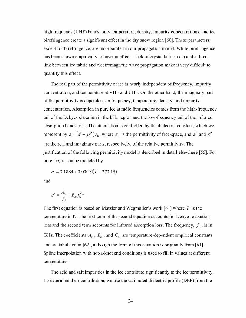
GISP2 ice cores and drill holes. The datasets used are shown in Fig. 2-1 and Fig. 2-2

along with references to the data. Each dataset was not available for the full length of the

core. The density data start at the top surface and extend to 1500 m. The density profile is

extended to the bedrock with a constant value equal to the average density in the last 100

m of valid data. The same technique is used to extend the beginning and end of the DEP

profile. The temperature profile is linearly extrapolated to the bed using the last 100 m of

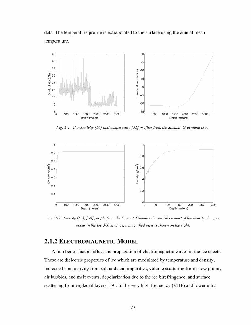
23

data. The temperature profile is extrapolated to the surface using the annual mean

temperature.

0 500 1000 1500 2000 2500 30005

10

15

20

25

30

35

40

45

Depth (meters)

Con

duct

ivity

(uS

/m)

0 500 1000 1500 2000 2500 3000-35

-30

-25

-20

-15

-10

-5

0

Depth (meters)

Tem

pera

ture

(Cel

cius

)

Fig. 2-1. Conductivity [56] and temperature [52] profiles from the Summit, Greenland area.

0 500 1000 1500 2000 2500 3000

0.4

0.5

0.6

0.7

0.8

0.9

1

Depth (meters)

Den

sity

(g/c

m3 )

0 50 100 150 200 250 3000

0.2

0.4

0.6

0.8

1

Depth (meters)

Den

sity

(g/c

m3 )

Fig. 2-2. Density [57], [58] profile from the Summit, Greenland area. Since most of the density changes

occur in the top 300 m of ice, a magnified view is shown on the right.

2.1.2 ELECTROMAGNETIC MODEL A number of factors affect the propagation of electromagnetic waves in the ice sheets.

These are dielectric properties of ice which are modulated by temperature and density,

increased conductivity from salt and acid impurities, volume scattering from snow grains,

air bubbles, and melt events, depolarization due to the ice birefringence, and surface

scattering from englacial layers [59]. In the very high frequency (VHF) and lower ultra

24

high frequency (UHF) bands, only temperature, density, impurity concentrations, and ice

birefringence create a significant effect in the dry snow region [60]. These parameters,

except for birefringence, are incorporated in our propagation model. While birefringence

has been shown empirically to have an effect – lack of crystal lattice data and a direct

link between ice fabric and electromagnetic wave propagation make it very difficult to

quantify this effect.

The real part of the permittivity of ice is nearly independent of frequency, impurity

concentration, and temperature at VHF and UHF. On the other hand, the imaginary part

of the permittivity is dependent on frequency, temperature, density, and impurity

concentration. Absorption in pure ice at radio frequencies comes from the high-frequency

tail of the Debye-relaxation in the kHz region and the low-frequency tail of the infrared

absorption bands [61]. The attenuation is controlled by the dielectric constant, which we

represent by ( ) 0εjεεε ′′−′= , where 0ε is the permittivity of free-space, and ε ′ and ε ′′

are the real and imaginary parts, respectively, of the relative permittivity. The

justification of the following permittivity model is described in detail elsewhere [55]. For

pure ice, ε can be modeled by

( )15.27300091.01884.3 −+=′ Tε

and

mCGm

G

m fBfA

+=′′ε .

The first equation is based on Matzler and Wegmüller’s work [61] where T is the

temperature in K. The first term of the second equation accounts for Debye-relaxation

loss and the second term accounts for infrared absorption loss. The frequency, Gf , is in

GHz. The coefficients mA , mB , and mC are temperature-dependent empirical constants

and are tabulated in [62], although the form of this equation is originally from [61].

Spline interpolation with not-a-knot end conditions is used to fill in values at different

temperatures.

The acid and salt impurities in the ice contribute significantly to the ice permittivity.

To determine their contribution, we use the calibrated dielectric profile (DEP) from the

25

GRIP ice core. The DEP-derived conductivity profile from GRIP gives the high-

frequency limit of conductivity measured at LF and corrected to 258 K [63]. Fujita et al.

[55] suggest that the high-frequency limit conductivity is valid at our frequencies since

the molar conductivity does not change from LF to UHF.

The DEP-derived conductivity is sensitive to the Debye-relaxation and impurities, but

not infrared absorption. Therefore, we use the conductivity profile only to estimate the

impurity component of conductivity. Because of this, we need to subtract off the LF pure

ice conductivity. Using the single-frequency Debye model [63] suggests this value to be 9 1mµS −⋅ at 258 K. Due to errors in the conductivity profile, there are a few points in the

profile where the total conductivity is measured to be less than 9 1mµS −⋅ , leading to a

negative conductivity due to impurities. We set the impurity-component of the

conductivity to zero in these cases.

To determine the conductivity at other temperatures, we use an Arrenhius model (e.g.,

eqn. 3 of [64]):

−= ∞∞ TTR

E 11exp258

258,σσ

where 258,∞σ is the impurity-component of the conductivity from the profile,

eV22.0=E ( )-1molJ217,21 ⋅ is the activation energy suggested by [63], -1-1 KmolJ3144.8 ⋅⋅=R is the universal gas constant, T is the desired temperature in

Kelvin, and K258258=T is the temperature that the conductivity profile is given for. The

conductivity is related to the imaginary part of the permittivity by 02 επ

σεf∞=′′ where f is

the frequency in Hz.

The above equations are for solid ice with a density of 3mkg917 −⋅=iced . However,

the density of the ice sheet is a function of depth in the firn/ice transition region. To

account for a density of d , we scale the real part of the permittivity by [65]

26

2

2

7.07.117.07.11

iceice ddddD

++

++=′ ,

and the imaginary part of the permittivity by [65]

2

2

62.052.062.052.0

iceice ddddD

+

+=′′ .

Several issues regarding the accuracy of the permittivity must be dealt with. Fujita et

al. estimates the real part of the permittivity to be accurate to 1% based on the scatter of

available data [55]. The accuracy of the real part limits the maximum length of the SAR

aperture that can be coherently processed since phase coherence across the entire aperture

is required. We set the maximum acceptable phase error to be one eighth of a

wavelength. This corresponds to a signal-to-noise degradation of 0.2 dB. The maximum

synthetic apertures are 349 m, 248 m, and 177 m for 1%, 2%, and 4% velocity errors3.

Since hyperbolas have been observed in the bed echoes, auto-focusing techniques [66],

[67], [68], [69], [70], [71], [72] may improve the SAR’s performance and should be

investigated in the future.

The imaginary part of the permittivity, which determines the loss, has significant

error bars. An example for NGRIP, Greenland is given in [60] where the difference in

two-way ice loss predicted by two different sets of laboratory data for ice permittivity is

approximately 30 dB. Based on this large discrepancy, we proposed to perform common

midpoint measurements (CMP) utilizing a bistatic configuration to reduce the error bars

on the scattering strength estimates. Unfortunately, due to system design failures

described in section 7.3, the quality of the CMP data taken by the radar system was

insufficient for analysis. However, once these failures are corrected, the radar system is

capable of acquiring bistatic CMP data which could significantly reduce error bars.

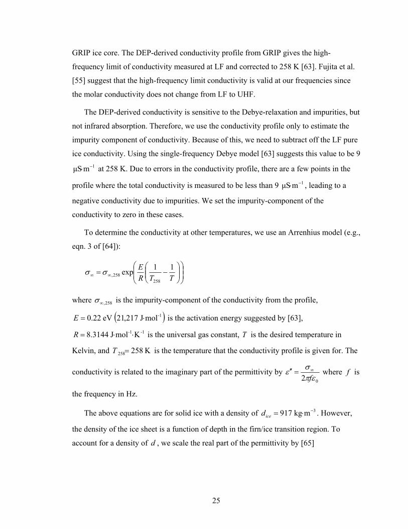
The real part of the permittivity at 210 MHz4 versus depth is shown in Fig. 2-3a. The

loss in -1kmdB ⋅ versus depth at 210 MHz is plotted in Fig. 2-3b.

3 For small errors, a velocity error of Verr% corresponds to a permittivity error of 2Verr%. 4 210 MHz is the center frequency used by the radar system.

27

0 500 1000 1500 2000 2500 30001.6

1.8

2

2.2

2.4

2.6

2.8

3

3.2

Depth (m)

Rea

l Per

mitt

ivity

e'

a)

0 500 1000 1500 2000 2500 30000

10

20

30

40

50

60

70

Depth (m)

Two-

way

Los

s (d

B/k

m)

b)

Fig. 2-3. The a) real part and b) imaginary part of the permittivity (expressed as loss) corresponding to the

geophysical profiles shown in Fig. 2-1 and Fig. 2-2.

As mentioned above, to acquire more accurate velocity and attenuation profiles, the

radar system will be designed so that it can operate in bistatic mode for common

midpoint measurements (CMP). (Requirements imposed by bistatic operation are

delineated in section 3.5.) The ice properties can be found by analyzing the reflections

from the planarly stratified media at various depths as a function of antenna separation in

the CMP measurements. More details are provided in section 7.3.

Without CMP measurements, we must rely on a permittivity profile derived from

geophysical profiles. In areas where these direct measurements are not available, models

of geophysical properties can provide a rough estimate. The density profile can be found

from accumulation and mean surface temperatures [73]. Accumulation and temperature

maps are readily available for Greenland and Antarctica [74], [75]. The temperature

profile can be found from models of the geothermal heat flux and are also available for

the Greenland and Antarctic ice sheets [76], [77]. Impurity profiles must be extrapolated

from areas with known DEP measurements. This represents the largest unknown and,

depending on spatial variability and proximity to an existing dataset, may represent the

largest source of error.

With the permittivity profile, the solution for the propagation of a plane wave in the

media can be found in closed form [78], [79]. Using simple ray-tracing approximations

and this discrete layer model, the phase delay, ray-path, and attenuation can be found for

28

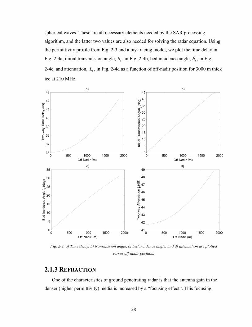
spherical waves. These are all necessary elements needed by the SAR processing

algorithm, and the latter two values are also needed for solving the radar equation. Using

the permittivity profile from Fig. 2-3 and a ray-tracing model, we plot the time delay in

Fig. 2-4a, initial transmission angle, tθ , in Fig. 2-4b, bed incidence angle, iθ , in Fig.

2-4c, and attenuation, tL , in Fig. 2-4d as a function of off-nadir position for 3000 m thick

ice at 210 MHz.

0 500 1000 1500 200036

37

38

39

40

41

42

43

Off Nadir (m)

Two-

way

Tim

e D

elay

(us)

a)

0 500 1000 1500 2000

0

5

10

15

20

25

30

35

40

45

Off Nadir (m)

Initi

al T

rans

mis

sion

Ang

le θ t (

deg)

b)

0 500 1000 1500 20000

5

10

15

20

25

30

35

Off Nadir (m)

Bed

Inci

denc

e A

ngle

θ i (

deg)

c)

0 500 1000 1500 200041

42

43

44

45

46

47

48

49

Off Nadir (m)

Two-

way

Atte

nuat

ion

L t (dB

)

d)

Fig. 2-4. a) Time delay, b) transmission angle, c) bed incidence angle, and d) attenuation are plotted

versus off-nadir position.

2.1.3 REFRACTION One of the characteristics of ground penetrating radar is that the antenna gain in the

denser (higher permittivity) media is increased by a “focusing effect”. This focusing

29

effect will be referred to as refraction gain, fG . For ice sheets, which tend to start at a

low permittivity near the surface and asymptotically approach a higher permittivity, the

refraction gain is a function of both depth and angle of incidence. West and Demarest use

a ray-tracing technique to solve for the refraction gain of an antenna on an ice sheet [80].

To solve for the refraction gain analytically, West and Demarest assume the form of

the density profile to be:

( ) ( )RzVz i exp−∆=∆

where

∆ is the density as a function of depth,

i∆ is the density of pure ice, taken to be 0.917 3cmg −⋅ ,

V is a model parameter with units of density (always less than P )

R is a model parameter with units of inverse distance (always positive)

z is the elevation (always negative).

This exponential form for the density profile is justified for ice sheets in the paper. West

and Demarest use Robin et al.’s results to convert the density profile in to a permittivity

profile [81] (written here in terms of the index of refraction):

( ) ( )zzn ∆+= 854.01

Since the permittivity conversion used in this work uses Tiuri’s results to convert density

to permittivity [65], the refraction gain has been re-derived for this case. Additionally,

there are a number of typographical mistakes in the paper that have been corrected here

(the corrected equations using Robin’s results are also included in parenthesis where they

differ from the equations for Tiuri’s results). This proof makes use of a change of

variables and two of Gradshteyn and Ryzhik’s integral solutions [82]. The refraction gain

is

( )γ

θ

θθ′

′′

=cos

sin,2

i

ttf

drdr

DzG

where

30

227.07.1 ζ−∆+∆+= ii CCCa or ( ( ) 22854.01 ζ−∆+= ia ),

VCCVb i∆−−= 4.17.1 or ( ( ) 854.0854.012 ib ∆+−= ),

27.0 CVd = or ( 2854.0=d ),

1=C is a scaling factor to Tiuri’s permittivity equation,

( ) tn θζ sin0= ,

( )RzVM exp= ,

( ) 2•+•+=• dbaX ,

( )( )( )( )( )abVVaXM

abMMaXVaRzn

zdrz

2222

ln0

22 ++++

−=−′

′=′ ∫

ζζ

ζ ,

22 zrD +′= ,

24 badq −= ,

( ) ( )( )

=′ −

tznnz θγ sin0sin 1 ,

and

( )( ) ( )

+−−

+−−

′+′=

′VX

badbdVMX

badbdMaqa

RrR

nrd

rd ii

i

222 222cos0cotζ

θζθθ

.

Before applying these results, we need to fit our density data to the exponential

function and find V and R . To do this, we take the natural log of ∆ to obtain a linear

relationship with respect to z

( )( ) ( ) RzVzi +=∆−∆ lnln .

We then fit a first order polynomial to the log density data using the least squares

technique. From the permittivity data presented in Fig. 2-3, 601.0=V and 0253.0−=R .

The RMS percentage error between the exponential fit and the data is less than 1%. A

plot of the refraction gain at normal incidence as a function of depth is shown in Fig.

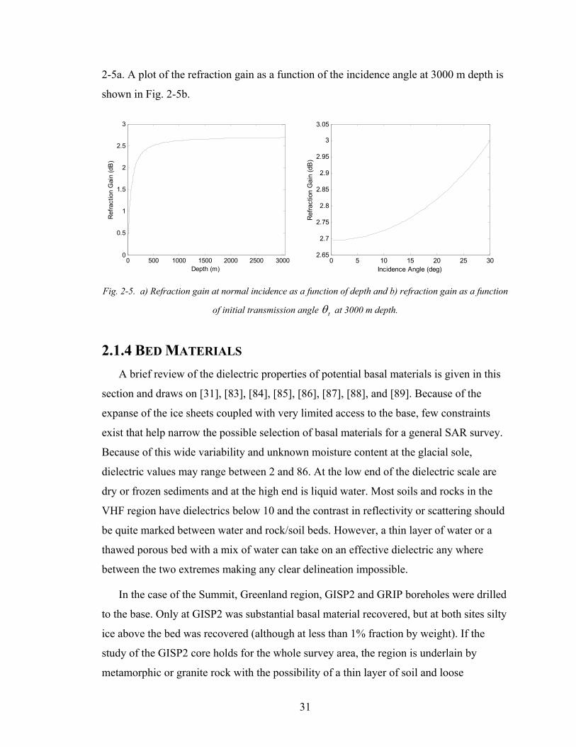
31

2-5a. A plot of the refraction gain as a function of the incidence angle at 3000 m depth is

shown in Fig. 2-5b.

0 500 1000 1500 2000 2500 30000

0.5

1

1.5

2

2.5

3

Depth (m)

Ref

ract

ion

Gai

n (d

B)

0 5 10 15 20 25 302.65

2.7

2.75

2.8

2.85

2.9

2.95

3

3.05

Incidence Angle (deg)

Ref

ract

ion

Gai

n (d

B)

Fig. 2-5. a) Refraction gain at normal incidence as a function of depth and b) refraction gain as a function

of initial transmission angle tθ at 3000 m depth.

2.1.4 BED MATERIALS A brief review of the dielectric properties of potential basal materials is given in this

section and draws on [31], [83], [84], [85], [86], [87], [88], and [89]. Because of the

expanse of the ice sheets coupled with very limited access to the base, few constraints

exist that help narrow the possible selection of basal materials for a general SAR survey.

Because of this wide variability and unknown moisture content at the glacial sole,

dielectric values may range between 2 and 86. At the low end of the dielectric scale are

dry or frozen sediments and at the high end is liquid water. Most soils and rocks in the

VHF region have dielectrics below 10 and the contrast in reflectivity or scattering should

be quite marked between water and rock/soil beds. However, a thin layer of water or a

thawed porous bed with a mix of water can take on an effective dielectric any where

between the two extremes making any clear delineation impossible.

In the case of the Summit, Greenland region, GISP2 and GRIP boreholes were drilled

to the base. Only at GISP2 was substantial basal material recovered, but at both sites silty

ice above the bed was recovered (although at less than 1% fraction by weight). If the

study of the GISP2 core holds for the whole survey area, the region is underlain by

metamorphic or granite rock with the possibility of a thin layer of soil and loose

32

sediments and the bed is 6 C below the pressure melting point. Since the bed is frozen to

its base, large variations in backscatter are probably due to changes in roughness and

surface slope rather than dielectric contrasts.

Although the GISP2 and GRIP sites are unlikely to present a chance to test the

existence of subglacial water, one of the most important applications of a subglacial

imaging radar is to detect the presence of basal water. We start by illustrating the results

for normal incidence using a 3-layer model involving ice, water, and bed material [90].

The permittivity of ice is found using the techniques described in section 2.1.2 and is

taken to be 15.3=iceε . The water permittivity is found using a Debye relationship [91]

w

wwww fj τπ

εεεε21

0

+−

+= ∞∞ ,

where

9.4=∞wε ,

35240 10075.110295.64147.0045.88 TTTw

−− ×+×+−=ε ,

3162141210 10096.510938.610824.3101109.12 TTTw−−−− ×−×+×−×=πτ ,

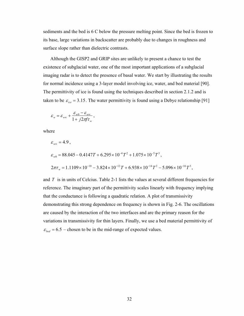
and T is in units of Celcius. Table 2-1 lists the values at several different frequencies for

reference. The imaginary part of the permittivity scales linearly with frequency implying

that the conductance is following a quadratic relation. A plot of transmissivity

demonstrating this strong dependence on frequency is shown in Fig. 2-6. The oscillations

are caused by the interaction of the two interfaces and are the primary reason for the

variations in transmissivity for thin layers. Finally, we use a bed material permittivity of

5.6=bedε – chosen to be in the mid-range of expected values.

33

Table 2-1: Permittivity of water at several frequencies. Frequency

(MHz)

Real Part

wε ′

Imaginary Part

wε ′′

150 88.02 1.39

300 87.95 2.77

450 87.84 4.15

650 87.61 5.97

0 200 400 600 800 1000-50

-40

-30

-20

-10

0a)

Water Layer Thickness (mm)

Tran

smis

sivi

ty (d

B)

150 MHz300 MHz450 MHz650 MHz

0 1 2 3 4 5-6

-5

-4

-3

-2

-1b)


Tran

smis

sivi

ty (d

B)150 MHz300 MHz450 MHz650 MHz

Fig. 2-6. a) Plot of transmissivity through basal water layer at normal incidence, b) Magnified view of

transmissivity for thin layers.

The reflectance at normal incidence (depth sounding mode) is shown in Fig. 2-7 at

several frequencies as a function of water layer thickness. These results suggest that only

a 1-4 mm layer thickness is enough to change the reflectance by 6 dB depending on the

frequency of operation. The reflectivity variation is strongly dependent on the

constructive/destructive interference pattern. These results are of course valid when the

basal interface is a planar interface, but they are also valid when the large RMS height

physical optics model holds (see section 2.4). To a lesser extent they are valid for the

small-slopes physical optics model since Fresnel reflections are the basis of the

scattering, but this model does not directly incorporate the Fresnel reflection coefficient.

The effect is less obvious on surfaces for which the small perturbation model is valid.

One approach is to use radiative transfer theory for layered rough interfaces laid out by

Fung [92]. This approach is very technical and a simplified approach is used here so the

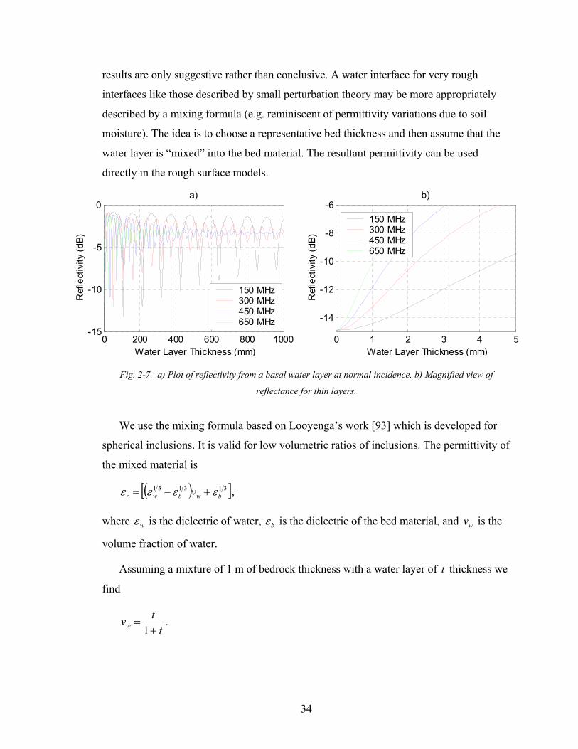
34

results are only suggestive rather than conclusive. A water interface for very rough

interfaces like those described by small perturbation theory may be more appropriately

described by a mixing formula (e.g. reminiscent of permittivity variations due to soil

moisture). The idea is to choose a representative bed thickness and then assume that the

water layer is “mixed” into the bed material. The resultant permittivity can be used

directly in the rough surface models.

0 200 400 600 800 1000-15

-10

-5

0a)


Ref

lect

ivity

(dB

)


0 1 2 3 4 5

-14

-12

-10

-8

-6b)


Ref

lect

ivity

(dB

)


Fig. 2-7. a) Plot of reflectivity from a basal water layer at normal incidence, b) Magnified view of

reflectance for thin layers.

We use the mixing formula based on Looyenga’s work [93] which is developed for

spherical inclusions. It is valid for low volumetric ratios of inclusions. The permittivity of

the mixed material is

( )[ ]313131bwbwr v εεεε +−= ,

where wε is the dielectric of water, bε is the dielectric of the bed material, and wv is the

volume fraction of water.

Assuming a mixture of 1 m of bedrock thickness with a water layer of t thickness we

find

ttvw +

=1

.

35

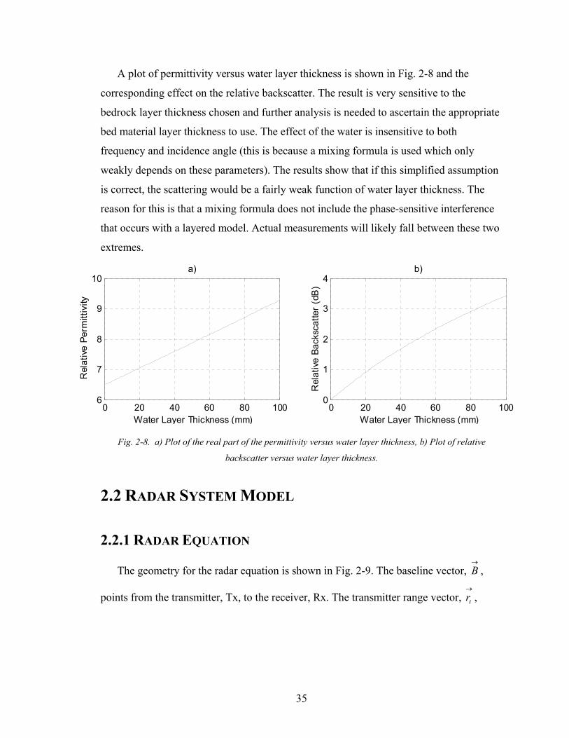
A plot of permittivity versus water layer thickness is shown in Fig. 2-8 and the

corresponding effect on the relative backscatter. The result is very sensitive to the

bedrock layer thickness chosen and further analysis is needed to ascertain the appropriate

bed material layer thickness to use. The effect of the water is insensitive to both

frequency and incidence angle (this is because a mixing formula is used which only

weakly depends on these parameters). The results show that if this simplified assumption

is correct, the scattering would be a fairly weak function of water layer thickness. The

reason for this is that a mixing formula does not include the phase-sensitive interference

that occurs with a layered model. Actual measurements will likely fall between these two

extremes.

0 20 40 60 80 1006

7

8

9

10


Rel

ativ

e Pe

rmitt

ivity

a)

0 20 40 60 80 1000

1

2

3

4


Rel

ativ

e Ba

cksc

atte

r (d

B)

b)

Fig. 2-8. a) Plot of the real part of the permittivity versus water layer thickness, b) Plot of relative

backscatter versus water layer thickness.

2.2 RADAR SYSTEM MODEL

2.2.1 RADAR EQUATION

The geometry for the radar equation is shown in Fig. 2-9. The baseline vector, →

B ,

points from the transmitter, Tx, to the receiver, Rx. The transmitter range vector, →

tr ,

36

points from the transmitter to the target. The transmitter range then is 2

→

= tt rR .5

Likewise, the receiver range vector, →

tr , points from the receiver to the target and the

receiver range is 2

→

= rr rR . T is the transmitter’s and receiver’s height above the target.

Not shown are the polarization directions of the transmit antenna, tη , and receive

antenna, rη . Using the ordinary definitions of →

iθ and →

iφ in the spherical coordinate

system, tη is the angle the E-plane6 of the antenna makes with the plane defined by the

vector →

iθ and →

iφ at the target. →

iθ is the origin and tη increases toward →

iφ . For

reference, 0=tη implies that the polarization at the target is purely vertical and 2πη =t

implies the polarization is horizontal. rη is likewise defined with respect to →

sθ and →

sφ .

When referring to a particular Cartesian component of a vector, e.g. →

tr , we use the

following notation [ xrt =1, , yrt =2, , zrt =3, ].

Fig. 2-9. The geometry used for the radar equation.

5

2• is the two-norm or Euclidean distance.

6 The E-plane contains the E-field at the target and the antenna’s position.

37

The radar system remotely senses the basal conditions of the ice sheet by illuminating

the bed and measuring the radiated fields from the induced currents on the bed. The

radiated fields from the ice-bed interface can be divided into coherent and incoherent

components. The coherent component, also known as the specular response, is generated

from currents that are correlated over the entire illuminated area. This component is

described by Fresnel reflection theory. Incoherent scattering is radiation from the

uncorrelated part of the currents. We will start by deriving the area-extensive form of the

radar equation (incoherent form) and then specialize it to its specular or coherent

scattering form.

The radar equation for an area extensive target gives the expectation of the power

received from a single pixel or resolution cell in terms of radar, medium, and target

parameters. The radar equation is a function of the frequency, f , and system geometry

parameters, rR , tR , tθ , tφ , rθ , rφ , iθ , iφ , sθ , sφ , tη , and rη :

( ) ( ) ( ) ( )

( ) ( )( )2

2

02

4,,,,

,,,,,,,,4

,,

rice

rrrrrr

rtssiitttt

ttttr

RfncfGRfL

fARfLRfGfPP

πφθθ

ηηφθφθσθπ

φθ=

Each of the components of this equation is described in the paragraphs below. This is a

generalization of the description given by Ulaby et al. [90].

The first term in the equation, ( ) ( )24

,,

t

tttt

RfGfP

πφθ , represents the average power

density of the transmitted wave at the target. tP is the transmitted power and is

determined by the DDS generated waveform and the transfer function of the transmitter.

tG is the gain of the transmit antenna network, which is a function of frequency and the

direction towards the target. The gain for the transmit antennas is found by using a finite

element numerical electromagnetic solver [95] to find the fields near the antenna on the

snow surface, 6.1, ≈snowrε . These results are extended to depth by using the results of

West and Demarest [80] as described in Appendix B.

38

The fifth term in the equation, ( )( )2,

2

4,,

rsnowr

rrr

fRcfG

πεφθ , represents the power coupled into the

receiver as a function of the power scattered. rG is the gain of the receive antenna

network and is found in the same way as for the transmit antenna network. c is the speed

of light in a vacuum.

The second and fourth terms, ( ) ( )

= ∫

−T

tztt dzzfRfL0

,,exp,, θαθ and

( ) ( )

= ∫

−T

rzrr dzzfRfL0

,,exp,, θαθ respectively, give the total extinction as the

electromagnetic wave travels through the media. The integral sums the loss from the

surface to the bedrock with an ice thickness of rrtt RRT θθ coscos ≈≈ 7. ( )zf tz ,,θα is

the extinction coefficient of the medium and is found using the ice sheet model detailed

in section 2.1. Since the ice sheet is modeled as an inhomogeneous medium with

constitutive parameters that are functions of depth only, for a plane wave source the

extinction coefficient’s only spatial dependence is on z . We model the point source

nature of our antenna by computing the plane wave solution for each angle of incidence.

The extinction coefficient changes as a function of the plane wave’s incidence angle.

Therefore, the extinction coefficient is a function of z and tθ for the incidence field and

rθ for the scattered field.

The third term, ( )rtssiifA ηηφθφθσ ,,,,,,0 , is the ratio of the power density at the

target to the total scattered power times the gain of the scattered energy in the direction of

the receiver. A is the size of the target pixel (backscatter is incoherent so power rather

than voltage or current is added as the area is increased). ( )rtssiif ηηφθφθσ ,,,,,,0 is the

scattering coefficient and is the ratio of the power density at the target to the total

scattered power from one unit area times the gain of the scattered energy in the direction

of the receiver. The scattering coefficient is found using a rough surface model. Since the

terrain below an ice sheet is so extensive, no one model can adequately explain the

scattering for the entire bed of the ice sheet. For this reason, the results from several

7 These are only approximations since the permittivity is a function of depth. The exact thickness is related to the incidence angle and range using a ray-tracing model.

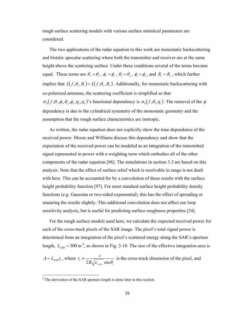
39

rough surface scattering models with various surface statistical parameters are

considered.

The two applications of the radar equation to this work are monostatic backscattering

and bistatic specular scattering where both the transmitter and receiver are at the same

height above the scattering surface. Under these conditions several of the terms become

equal. These terms are rt θθ = , rt φφ = , si θθ = , si φφ = , and rt RR = , which further

implies that ( ) ( )rrtt RfLRfL ,,,, θθ = . Additionally, for monostatic backscattering with

co-polarized antennas, the scattering coefficient is simplified so that

( )rtssiif ηηφθφθσ ,,,,,,0 ’s functional dependency is ( )tif ηθσ ,,0 . The removal of the φ

dependency is due to the cylindrical symmetry of the monostatic geometry and the

assumption that the rough surface characteristics are isotropic.

As written, the radar equation does not explicitly show the time dependence of the

received power. Moore and Williams discuss this dependency and show that the

expectation of the received power can be modeled as an integration of the transmitted

signal represented in power with a weighting term which embodies all of the other

components of the radar equation [96]. The simulations in section 3.3 are based on this

analysis. Note that the effect of surface relief which is resolvable in range is not dealt

with here. This can be accounted for by a convolution of these results with the surface

height probability function [97]. For most standard surface height probability density

functions (e.g. Gaussian or two-sided exponential), this has the effect of spreading or

smearing the results slightly. This additional convolution does not affect our loop

sensitivity analysis, but is useful for predicting surface roughness properties [24].

For the rough surface models used here, we calculate the expected received power for

each of the cross-track pixels of the SAR image. The pixel’s total signal power is

determined from an integration of the pixel’s scattered energy along the SAR’s aperture

length, m300=SARL 8, as shown in Fig. 2-10. The size of the effective integration area is

cSARrLA = , where iicer

c Bcr

θε sin2 ,

≈ is the cross-track dimension of the pixel, and

8 The derivation of the SAR aperture length is done later in this section.

40

MHz180=B is the bandwidth. Since the radar and scattering parameters are functions

of the radar’s position in the SAR aperture, the area is subdivided into smaller areas over

which these parameters are essentially constant. Various rough surface models are

reviewed and their results using the radar equation developed here are given in section

2.4.

Fig. 2-10. The SAR imaging geometry. The along-track direction is x, the cross-track or ground range

direction is y, and the elevation is z. The radar’s synthetic aperture length is SARL . The dimensions of a

single pixel are cr by ar .

2.2.2 SPECULAR RADAR EQUATION For a specular surface, transmitter and receiver a fixed distance above the surface

implying tr RR = , and a planarly stratified media implying tr LL = , the radar equation

simplifies to

( ) ( ) ( )( )

( ) 2222

2

,,64

,,,,ppttt

tice

rrrttttr RfL

RfncfGfGfPP Γ= θ

πφθφθ .

This equation follows from an application of image theory [98] which translates the radar

geometry into an equivalent direct path geometry.

41

If a rough interface is sufficiently smooth, it can also be approximated by a planar

interface [99], [100], [101]. In this case, the scattering follows a modified Fresnel

reflection. For both horizontal and vertical polarization, the modification takes the form

of a power reflection coefficient weighting according to ( )222 sin2exp hk iθ− . Letting 2sΓ

be the Fresnel reflection coefficient for a flat surface, then the modified Fresnel

coefficient is given by

( )22222 sin2exp hk iss θ−Γ=Γ

Note that the modified Fresnel coefficient is the average or expected power reflection

coefficient where the expectation is taken over the ensemble of surface functions.

2.3 INTERNAL LAYERS

The specular radar equation is used to describe the scattering from layers within the

ice sheet. These layers are known as isochrones because they are caused by snow

deposition that occurred in the same time frame over a large area. Three primary causes

of reflections have been hypothesized in the literature: density changes, acidity changes,

and ice crystal fabric changes between layers [55]. While all three undoubtedly occur,

only the former two have been directly matched to radar reflections [102], [103]9. Using

this ice sheet model and observations from previous field work, a range of expected

power reflections from these layers is given in this section.

Density changes in the ice sheet through two mechanisms. The first is caused by

seasonal changes in temperature and accumulation rate and the other is due to the ice

overburden pressure which transforms snow into ice as the snow is buried deeper in the

ice sheet by new accumulation. These density changes are responsible for most of the

reflections in the top of the ice sheet, but do not show up below about 300 m, since at this

point the snow has been compacted into ice. As reported earlier in this chapter, the

density is almost linearly related to the real and imaginary parts of the permittivity. Since

the real part of the permittivity is many orders of magnitude greater than the imaginary 9 A number of attempts have been made to characterize the effects of crystal fabric on radar returns [104], [105], [106], [107], [108], [109], [110], [111], [112], [113], [114], [115], but no work has made a conclusive link.

42

part, these reflections are real as opposed to complex and not functions of frequency

(closely spaced layers can create frequency dependency through constructive and

destructive interference) [55].

Impurity concentration changes relate to the atmospheric conditions when the snow

was deposited. For example, large volcanoes or volcanoes in close proximity increase the

amount of sulfuric acid in the atmosphere above the ice sheet. These impurities are

deposited with the snow and change the snow’s conductivity. The impurities migrate very

slowly in the snow once deposited and therefore can be observed to the bed of the ice

sheet where the oldest snow lies. Since only the conductivity changes, these reflections

are imaginary and are functions of frequency [55].

To determine our instantaneous dynamic range requirements and the loop sensitivity,

we need to know the expected strength of the reflection from these layers as a function of

depth. Using the ice model described in section 2.1 and the specular radar equation, the

predicted impulse response of a point source is plotted in Fig. 2-11a. These values are

significantly lower than what has been observed in the field. The main problem is that the

sampling rate of the geophysical profiles is 0.5-1 m at best and the parameters are

averaged measurements over this length. Because of the low pass filtering and under-

sampling of the original data, much of the high-frequency permittivity changes are

removed and proper re-interpolation to a common depth axis is problematic. A filtered set

of previous field data, ( ) 2zfiltΓ , is plotted in Fig. 2-11b and is used for the loop

sensitivity and dynamic range calculations. A fourth degree polynomial, ( ) 2zpolyΓ , is

fitted to ( ) 2zfiltΓ using the least squares solution. If we make the assumption that any

reflection profile, ( ) 2zΓ , will satisfy

( ) ( ) ( ) 24224 1010 zzz polypoly Γ<Γ<Γ−

then we can constrain our dynamic range and loop sensitivity. The limits, ( ) 2410 zpolyΓ−

and ( ) 2410 zpolyΓ , along with the fitted polynomial ( ) 2zpolyΓ are plotted in Fig. 2-11b.

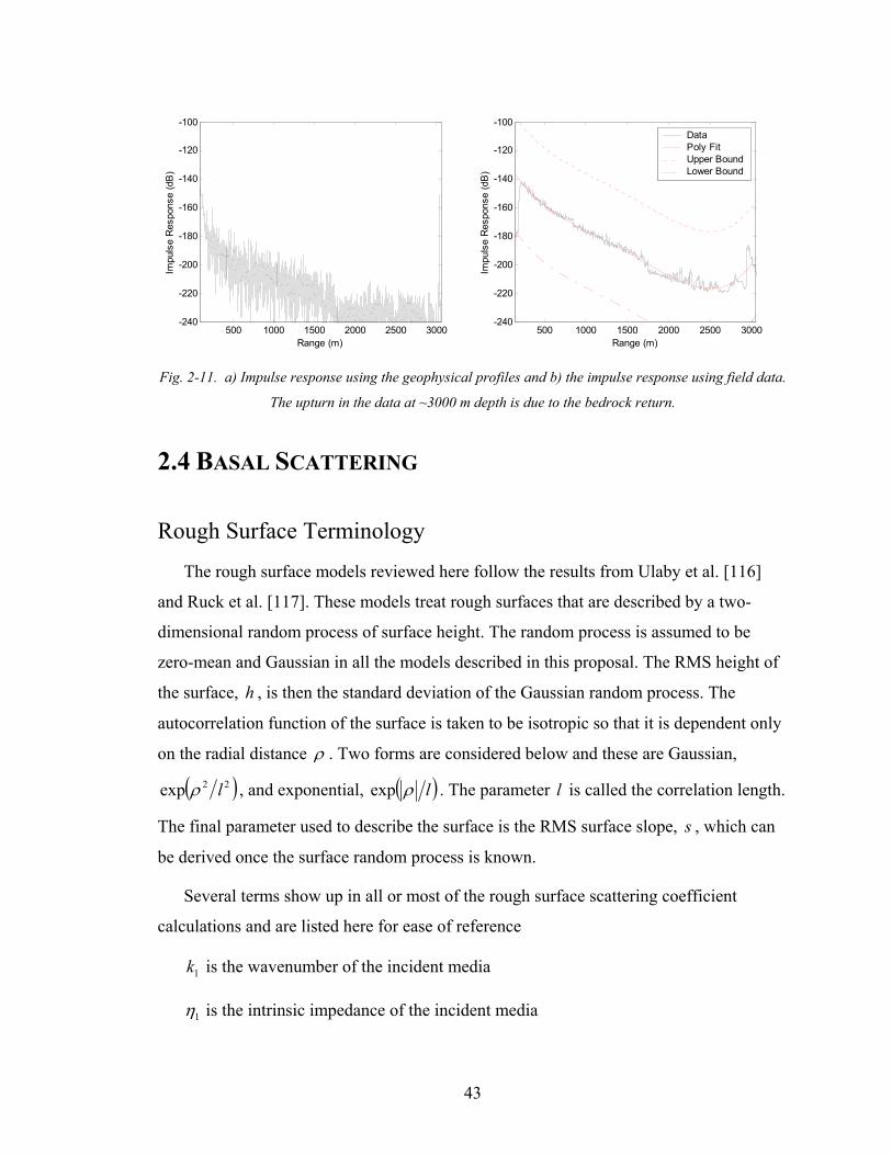
43

500 1000 1500 2000 2500 3000-240

-220

-200

-180

-160

-140

-120

-100

Range (m)

Impu

lse

Res

pons

e (d

B)

500 1000 1500 2000 2500 3000

-240

-220

-200

-180

-160

-140

-120

-100

Range (m)

Impu

lse

Res

pons

e (d

B)

DataPoly FitUpper BoundLower Bound

Fig. 2-11. a) Impulse response using the geophysical profiles and b) the impulse response using field data.

The upturn in the data at ~3000 m depth is due to the bedrock return.

2.4 BASAL SCATTERING

Rough Surface Terminology

The rough surface models reviewed here follow the results from Ulaby et al. [116]

and Ruck et al. [117]. These models treat rough surfaces that are described by a two-

dimensional random process of surface height. The random process is assumed to be

zero-mean and Gaussian in all the models described in this proposal. The RMS height of

the surface, h , is then the standard deviation of the Gaussian random process. The

autocorrelation function of the surface is taken to be isotropic so that it is dependent only

on the radial distance ρ . Two forms are considered below and these are Gaussian,

( )22exp lρ , and exponential, ( )lρexp . The parameter l is called the correlation length.

The final parameter used to describe the surface is the RMS surface slope, s , which can

be derived once the surface random process is known.

Several terms show up in all or most of the rough surface scattering coefficient

calculations and are listed here for ease of reference

1k is the wavenumber of the incident media

1η is the intrinsic impedance of the incident media

44

2k is the wavenumber of the media beneath the interface

2η is the intrinsic impedance of the media beneath the interface

( )iissx kq φθφθ cossincossin1 += ,

( )iissy kq φθφθ sinsinsinsin1 += ,

( )isz kq θθ coscos1 += ,

and

2222zyx qqqq ++= .

The equation for zq is incorrect in Ruck et al. Also, Ulaby et al.’s definition for iφ does

not match the standard coordinate spherical system definition as it is shifted by π (this is

not stated explicitly in their text). The correct form for zq is given here and the standard

definition of iφ is used. For monostatic (i.e. backscatter) these equations simplify to

iix kq φθ cossin2 1= ,

iiy kq φθ sinsin2 1= ,

and

iz kq θcos2 1= .

Although there is still a φ dependency, in all the scattering coefficient results below this

dependency cancels out in the backscattering case.

Finally, we must consider the antennas’ polarization. In all cases in this work, we are

interested in arbitrary linear polarization so this is the only type of polarization that will

be considered. Typically the incident and scattered fields are divided into horizontal and

vertical components. The scattered fields are then solved for with respect to each of these

components. Let pqα be the ratio of the q-polarized transmit field to the p-polarized

receive field. The principle of superposition allows us to add these four field components

together to find the ratio of the actual receiver to transmitter polarizations, rt ηηα , . The

45

apportionment between each of the components is dependent on the orientation of the

antennas, tη and rη , according to (Ruck et al.)

rthhrthvrtvhrtvvrtηηαηηαηηαηηαα ηη sinsinsincoscossincoscos, +++= .

Note that this result considers ratios of fields and not powers, whereas the scattering

coefficient represents ratios of powers.

Small Perturbation Model

The small perturbation model predicts the power scattered from a surface with a small

RMS height. A complete derivation of the monostatic (backscatter) result for a rough

surface satisfying the conditions described below and a Gaussian correlation coefficient

is given in Ulaby et al. Most of the derivation for the more general bistatic situation is

given as well. However, the surface power spectral density needed to calculate the

scattering coefficient is not provided. Ruck et al. present these results and their results

match Ulaby et al.’s where direct comparisons can be made. In addition, the result for an

exponential correlation function is also given in Ruck et al.

This surface model is applicable to surfaces which satisfy the following assumptions

1. Surface RMS height satisfies 3.00 <hk . (Ruck et al. suggests a slightly less restrictive

criteria with 10 <hk ). When determining h for this model, only the frequency

components of the surface responsible for scattering should be considered. These are

roughly the frequency components with wavelengths equal to the radar’s operating

wavelength.

2. Average surface slope, s , is less than 0.3. For a Gaussian correlation function, Ulaby

et al. shows that lhs 2= . (Ruck et al. suggests a slightly less restrictive criteria with

slope less than 1).

The scattering coefficient is given by

Ihk pqsipq

222241 coscos4 αθθ

πσ =

where

46

1k is the wave number of the incidence media,

rε is the permittivity of medium 2 relative to medium 1,

rµ is the permeability of medium 2 relative to medium 1,

( ) ( ) ( )[ ][ ]srrsrirrir

irrrrsrrrrisvh

θµεθεθµεθµ

θµεµεθµεεµφφα

22

22

sincossincos

sin1sin1sin

−+−+

−−−−−−= ,

( ) ( ) ( )[ ][ ]srrsrirrir

irrrrsrrrrishv

θµεθµθµεθε

θµεεµθµεµεφφα

22

22

sincossincos

sin1sin1sin

−+−+

−−−−−−= ,

( ) ( )( )( ) ( )

[ ][ ]srrsrirrir

isrr

srrirrissirr

vvθµεθεθµεθε

φφµε

θµεθµεφφθθεε

α22

2

22

sincossincos

cos1

sinsincossinsin1

−+−+

−−−

−−−+−

= ,

( )

+−=

4exp

2222 yx qql

lI π for a Gaussian correlation function,

and ( )[ ] 5.1222

2

112

yx qqllI

++= π for an exponential correlation function.

As a side note, Ulaby et al. has a sign error in vvα that has been corrected here and is

also correct in Ruck et al. Additionally, both Ulaby et al and Ruck et al assume πφ =i

and the equations above are generalized for arbitrary iφ . For monostatic or backscatter,

we note that

iyx kqq θ221

22 sin4=+

and the scattering coefficients for a Gaussian correlation function are

( ) ( )( ) ( )[ ] ( )i

irrir

rrrrirrihh kllhk θ

θµεθµ

εµµεθµµθσ 221

2

2

22

224224

1 sinexpsincos

1sin11cos4 −−+

−−+−−=

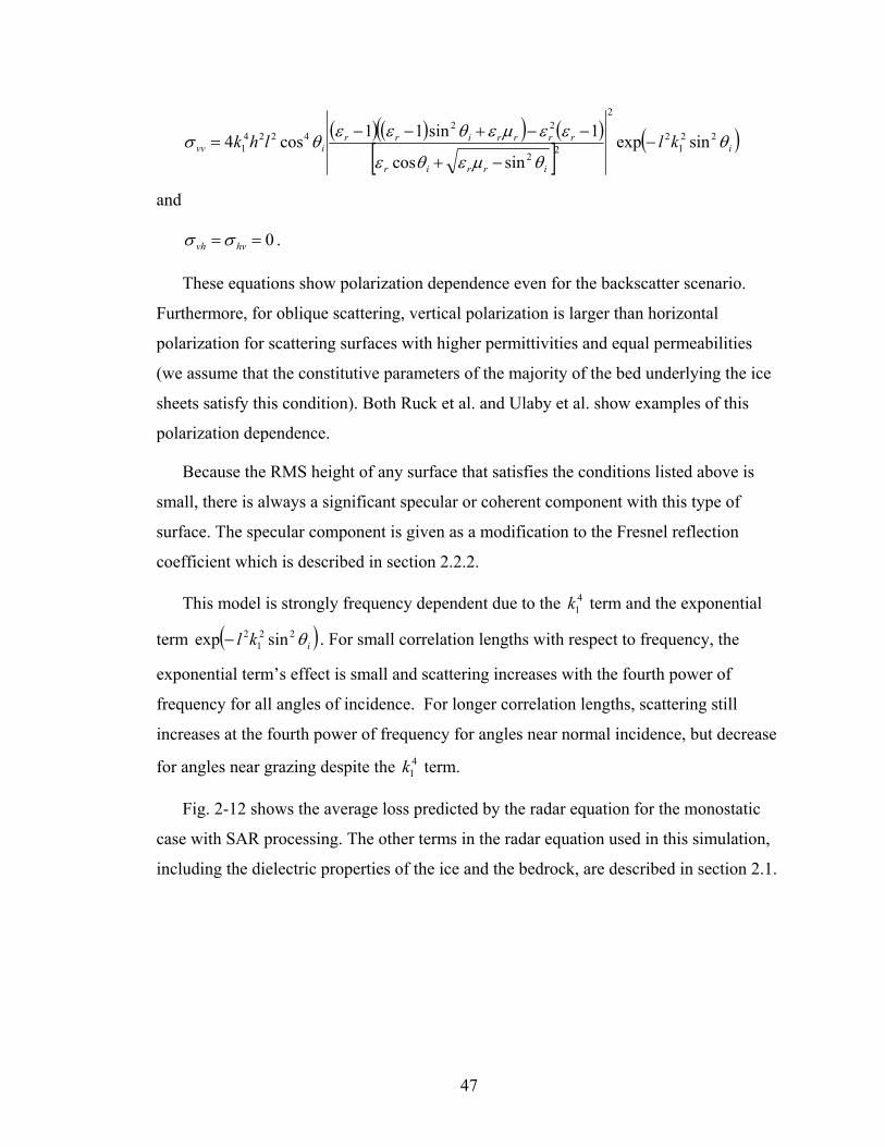
47

( ) ( )( ) ( )[ ] ( )i

irrir

rrrrirrivv kllhk θ

θµεθε

εεµεθεεθσ 221

2

2

22

224224

1 sinexpsincos

1sin11cos4 −−+

−−+−−=

and

0== hvvh σσ .

These equations show polarization dependence even for the backscatter scenario.

Furthermore, for oblique scattering, vertical polarization is larger than horizontal

polarization for scattering surfaces with higher permittivities and equal permeabilities

(we assume that the constitutive parameters of the majority of the bed underlying the ice

sheets satisfy this condition). Both Ruck et al. and Ulaby et al. show examples of this

polarization dependence.

Because the RMS height of any surface that satisfies the conditions listed above is

small, there is always a significant specular or coherent component with this type of

surface. The specular component is given as a modification to the Fresnel reflection

coefficient which is described in section 2.2.2.

This model is strongly frequency dependent due to the 41k term and the exponential

term ( )ikl θ221

2 sinexp − . For small correlation lengths with respect to frequency, the

exponential term’s effect is small and scattering increases with the fourth power of

frequency for all angles of incidence. For longer correlation lengths, scattering still

increases at the fourth power of frequency for angles near normal incidence, but decrease

for angles near grazing despite the 41k term.

Fig. 2-12 shows the average loss predicted by the radar equation for the monostatic

case with SAR processing. The other terms in the radar equation used in this simulation,

including the dielectric properties of the ice and the bedrock, are described in section 2.1.

48

0 200 400 600 800 1000-220

-210

-200

-190

-180

-170

-160

Cross-track Position (m)

Pt /

Pr (d

B)

h = 0.025, l = 1h = 0.0125, l = 1h = 0.0125, l = 0.5h = 0.025, l = 2

Fig. 2-12. Total loss at the radar’s center frequency, 210 MHz, predicted by the radar equation using the

small perturbation model for the bed surface. The results for four different surface characteristics are

plotted.

Physical Optics, Large RMS Heights Model

This physical optics model predicts the surface scattering from surfaces with large

radiuses of curvature and a large RMS height with respect to wavelength. The complete

derivation for this scattering model with Gaussian height and correlation surface statistics

is given in Ulaby et al. Ruck et al presents results for Gaussian and exponential

correlation coefficients. However, the results in Ruck et al include a factor of 2

everywhere the surface slope variance enters the equation. This error enters because Ruck

et al.’s RMS surface slope definition on page 705 has a factor of 2 error. For a correct

derivation, see pages 1011-2 from Ulaby et al. with ( ) 220 l−=′′ρ for the Gaussian

correlation function.

This surface model is applicable to surfaces which satisfy the following assumptions

3. Surface features are larger than a wavelength so that λ>l .

4. Surface RMS height is large with respect to wavelength 10>hqz .

49

5. Radius of curvature (derived on pages 1011-1013 of Ulaby et al.) for the surface is

large with respect to wavelength λπ>

62

2

hl .

The scattering coefficient is given by

( )( ) ( )

′′

+−

′′=

02exp

02 22

22

24

2

1

ρσρσ

ασ

z

yx

z

pqpq q

qqq

qk

where

( ) 2

222 20

ls σρσ ==′′ ,

( )isp φφθ −= sinsin1 ,

( )issp φφθ −−= sinsin2 ,

( ) siissip θθφφθθ sincoscoscossin3 −−−= ,

( ) siissip θθφφθθ cossincossincos4 −−= ,

= −

z

zli qk

qq

1

1

2cosθ (local angle of incidence),

≈ −

lilt kk θθ sinResin

2

11 (local angle of transmission),

( )ltli

ltlil θηθη

θηθηθcoscoscoscos

12

12

+−

=Γ⊥ ,

( )ltli

ltlil θηθη

θηθηθcoscoscoscos

21

21|| +

−=Γ ,

( ) ( )( )( )2

3211

4321||

ppqkppppqq

z

llzhh +

Γ+Γ= ⊥ θθ

α ,

( ) ( )( )( )2

3211

4123||

ppqkppppqq

z

llzvh +

Γ+Γ= ⊥ θθ

α ,

50

( ) ( )( )( )2

3211

2341||

ppqkppppqq

z

llzhv +

Γ+Γ= ⊥ θθ

α ,

and

( ) ( )( )( )2

3211

2143||

ppqkppppqq

z

llzvv +

Γ+Γ= ⊥ θθ

α .

For monostatic or backscatter, the scattering coefficient is found by taking the limit as

is θθ → when si φφ = 10. The result is reproduced here as

( ) ( )( ) i

i

vvhh θρσρσθ

σσ 42

2

22||

cos0202

tanexp0

′′

′′

−Γ

==

and

0== hvvh σσ .

Unlike the small perturbation model, the physical optics model for large RMS heights

has effectively no coherent component. This is because the RMS height extends over a

wavelength so that the distribution of random phases from the surface is nearly uniform

on 0 to 2π. Additionally, because of the stationary phase approximation used in Ulaby et

al.’s derivation, all the scattered power comes from localized specular scattering. In other

words, only portions of the surface oriented to give a specular response are included. For

backscatter, specular scattering implies normal incidence so that there is no polarization

dependence in this model.

The model is also referred to as the high frequency model because it applies for all

frequencies above a threshold value (see assumptions above). Fung shows that the

general integral equation method (IEM) model for rough surfaces converges to this model

in the high frequency limit [118]. Therefore, scattering predicted by this model is

frequency independent. (Although the wavenumber appears in this “edition” of the

equations, it always cancels out.)

10 The limit from only one direction needs to be considered because the scattering function is continuous almost everywhere and only one singular point in the finite plane exists.

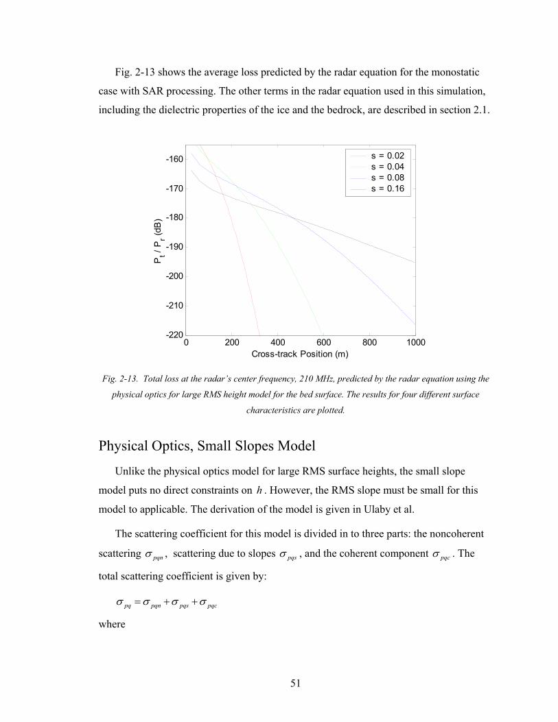
51




0 200 400 600 800 1000-220

-210

-200

-190

-180

-170

-160


Pt /

Pr (d

B)

s = 0.02s = 0.04s = 0.08s = 0.16


physical optics for large RMS height model for the bed surface. The results for four different surface

characteristics are plotted.

Physical Optics, Small Slopes Model

Unlike the physical optics model for large RMS surface heights, the small slope

model puts no direct constraints on h . However, the RMS slope must be small for this

model to applicable. The derivation of the model is given in Ulaby et al.

The scattering coefficient for this model is divided in to three parts: the noncoherent

scattering pqnσ , scattering due to slopes pqsσ , and the coherent component pqcσ . The

total scattering coefficient is given by:

pqcpqspqnpq σσσσ ++=

where

52

( ) ( ) ( )

+−−

= ∑

∞

= nlqq

nnqq

lk yx

n

nz

zpq

pqn 4exp

!exp

2

222

1

2222

2

,01 σσα

σ

( ) ( ) ( ) ( )

+−−−= ∑

∞

=

−

nlqq

nnqqqlk yx

n

nz

pqzz

pqpqs 4exp

!exp

2

222

1

1222

,1222

,01σασασ

( ) ( ) ( ) ( )222

,01 exp σδδαπσ zyxpqpqc qqqk −=

≈ −

it kk θθ sinResin

2

11 (local angle of transmission),

ti

tiRθηθηθηθη

coscoscoscos

12

120 +

−=⊥

ti

tiRRθηθηθηθη

coscossinsin

12

1201 +

+−= ⊥⊥

ti

tiRθηθηθηθη

coscoscoscos

21

210|| +

−=

( )ti

ittiRR

θηθηθηθηθηθη

coscossinsinsinsin

21

12210||1|| +

−++=

( ) ( )issihh R φφθθα −+−= ⊥ coscoscos0,0 ,

( )( ) ( ) ( )[ ]( )

+

−+−−−= ⊥⊥

iyix

isisisishhhh qq

RRφφ

φφθθφφθθαα

sincoscoscoscoscossinsin

Re*

1*

0,0,1 ,

( ) ( )issivh R φφθθα −+−= ⊥ sincoscos10,0 ,

( ) ( )[ ]( )

+

−+−−= ⊥⊥

iyix

issisivhvh qq

RRφφ

φφθθθθαα

sincossincoscos1cossin

Re*

1*

0,0,1 ,

( ) ( )issihv R φφθθα −+−= sincoscos10||,0 ,

( ) ( )[ ]( )

+

−+−−=

iyix

issisihvhv qq

RRφφ

φφθθθθαα

sincossincoscos1cossin

Re*1||

*0||,0

,1 ,

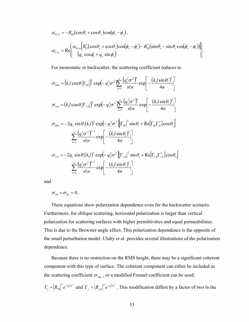
53

( ) ( )issivv R φφθθα −+−= coscoscos0||,0 ,

( ) ( ) ( )( )[ ]( )

+

−−−−+=

iyix

isisisisvvvv qq

RRφφ

φφθθφφθθαα

sincoscossinsincoscoscos

Re*0||

*1||,0

,1 .

For monostatic or backscatter, the scattering coefficient reduces to

( ) ( ) ( ) ( )

−−Γ= ∑

∞

= nlk

nnqqlk i

n

nz

zihhn 4sinexp

!expcos

21

1

22222

0||1θσσθσ

( ) ( ) ( ) ( )

−−Γ= ∑

∞

=⊥ n

lknn

qqlk i

n

nz

zivvn 4sinexp

!expcos

21

1

22222

01θσσθσ

( ) ( ) [ ]( ) ( )

−

ΓΓ+Γ−−=

∑∞

=

−

nlk

nnq

qlkq

i

n

nz

iizizhhs

4sinexp

!

cosResinexpsin22

1

1

122

*1||0||

20||

2221

θσ

θθσθσ

( ) ( ) [ ]( ) ( )

−

ΓΓ+Γ−−=

∑∞

=

−

⊥⊥⊥

nlk

nnq

qlkq

i

n

nz

iizizvvs

4sinexp

!

cosResinexpsin22

1

1

122

*10

20

2221

θσ

θθσθσ

and

0== hvvh σσ .

These equations show polarization dependence even for the backscatter scenario.

Furthermore, for oblique scattering, horizontal polarization is larger than vertical

polarization for scattering surfaces with higher permittivities and equal permeabilities.

This is due to the Brewster angle effect. This polarization dependence is the opposite of

the small perturbation model. Ulaby et al. provides several illustrations of the polarization

dependence.

Because there is no restriction on the RMS height, there may be a significant coherent

component with this type of surface. The coherent component can either be included as

the scattering coefficient pqcσ , or a modified Fresnel coefficient can be used:

2220||||

σzqeR −=Γ and 222

0σzqeR −

⊥⊥ =Γ . This modification differs by a factor of two in the

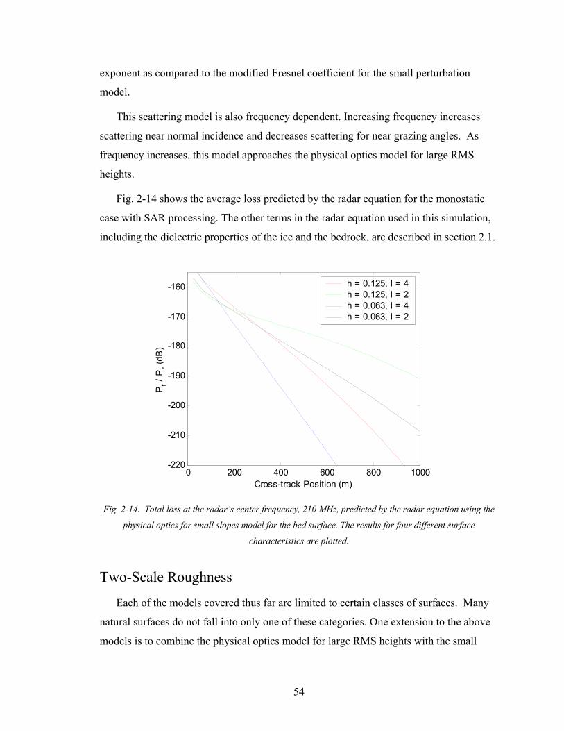
54

exponent as compared to the modified Fresnel coefficient for the small perturbation

model.

This scattering model is also frequency dependent. Increasing frequency increases

scattering near normal incidence and decreases scattering for near grazing angles. As

frequency increases, this model approaches the physical optics model for large RMS

heights.




0 200 400 600 800 1000-220

-210

-200

-190

-180

-170

-160


Pt /

Pr (d

B)

h = 0.125, l = 4h = 0.125, l = 2h = 0.063, l = 4h = 0.063, l = 2


physical optics for small slopes model for the bed surface. The results for four different surface

characteristics are plotted.

Two-Scale Roughness

Each of the models covered thus far are limited to certain classes of surfaces. Many

natural surfaces do not fall into only one of these categories. One extension to the above

models is to combine the physical optics model for large RMS heights with the small

55

perturbation model. This model can represent surfaces with two-scale roughness (a large

low frequency component and a small perturbation component). Ulaby et al. show that

for the proposed work where the angles of incidence are far from grazing, the solution for

this model is to simply add the scattering results of the two models together. The one

modification that is made to the large RMS height result is to use the small perturbation’s

modified Fresnel coefficients rather than the Fresnel coefficients for a flat surface. Note

that the small perturbation model has a coherent component which is not included in the

two-scale roughness model (the coherent component is effectively replaced by the

physical optics results).

56

Chapter 3: RADAR SYSTEM DESIGN

3.1 INTRODUCTION

The radar specifications are laid out in this chapter. The first section sets the general

frame-work (e.g. selection of a side-looking SAR) and lists constraints on the system

design such as size, coverage rate, etc. The next section details how the loop sensitivity

and dynamic range specifications were determined from simulation. This is followed by a

discussion of the antenna network. Finally, the requirements imposed by the bistatic

operation needed to provide CMP measurements are considered. In the final two sections,

a table summarizing the radar specifications and a set of block diagrams of the radar

system are given.

3.2 PRINCIPLE DESIGN DECISIONS

The initial framework for the radar design is a ground based side-looking synthetic

aperture radar. The ground-based operation provides flexibility and ease of testing as

compared to an airborne platform. Side-looking synthetic aperture radar enables the radar

to satisfy coverage and resolution requirements. Previous bedrock mapping missions

have for the most part been restricted to nadir-looking sounder operation. Musil’s work

near the grounding line on the Bach Ice Shelf is an exception [119], [120], [121]. This

system was operated along two very short traverses and for thin ice due to limitations of

available technology. The concept of side-looking operation has also been reviewed

briefly in [122]. Other efforts to apply synthetic aperture radar techniques have also been

reported in the literature, but these are all nadir-sounding [123], [124], [125], [126],

[127], [128], [129].

Ideally, the radar system would measure the full frequency spectrum with infinite

signal to interference and noise ratio. However, finite resources constrain the design and

concessions must be made. Due to design-time limitations we chose to use a proven

antenna design and digital system. The antenna we used is a TEM horn antenna [130],

57

[131]. The antenna dimensions could be scaled with frequency, but the weight and shape

of the antennas set a limit to the maximum number of elements and the minimum spacing

between elements. The digital system uses a direct digital synthesis (DDS) waveform

generator which can produce a fixed set of simple functions (e.g. linear FM chirp). The

data acquisition system set the dynamic range, the maximum throughput (a function of

PRF, sample word size, and number of samples), the maximum number of

simultaneously sampled channels, and the maximum sampling frequency. For shipping

and mobility considerations, the maximum cross-track dimension of the antenna network

was set to be 4 m. Likewise, the maximum along-track dimension of the antenna

network was set to 10 meters.

To achieve wide-area coverage in a reasonable time-frame, we chose a minimum

coverage rate of 12 hourkm10 −⋅ . Due to vehicle limitations, our platform velocity is 1sm3~ −⋅ , so our total swath width needs to be km1~ . Due to the high loss through the

ice and the low backscatter expected in some regions (details given later in this section),

the maximum cross-track distance to an image pixel must be less than or equal to

km1 from the radar. Considering that a side-looking radar cannot image in the nadir

direction because the ground-range resolution goes to infinity for normal incidence11, to

meet the coverage rate requirement the radar should image both sides of the platform to

achieve our desired total swath width. By imaging both sides of the platform

simultaneously rather than just one side, the effective swath width is doubled as shown in

Fig. 3-1. Since we additionally require nadir sounding and broadband operation, a cross-

track antenna array with multiple transmit and receive channels is used. With multiple

channels we can apply spatial filters to focus the beam towards nadir for depth sounder

data collection while simultaneously steering beams to the left and right side of the

platform for side-looking data collection. Additionally, digitally combining channels

circumvents the problem of controlling the antenna’s radiation pattern over a broad

11 The cross-track resolution is

i

cc

vrθ

τsin2

= , where v is the speed of electromagnetic waves in the

media, cτ is the compressed pulse width of the radar , and iθ is the incidence angle [132].

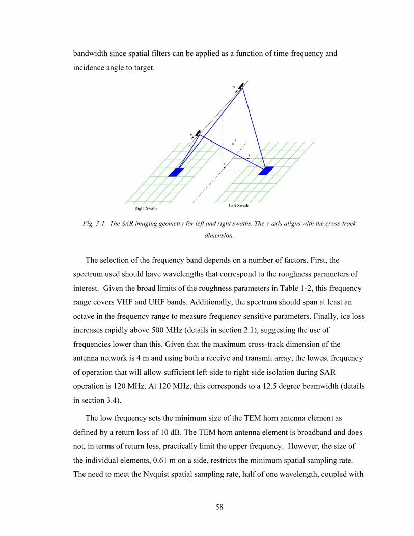
58

bandwidth since spatial filters can be applied as a function of time-frequency and

incidence angle to target.

Fig. 3-1. The SAR imaging geometry for left and right swaths. The y-axis aligns with the cross-track

dimension.

The selection of the frequency band depends on a number of factors. First, the

spectrum used should have wavelengths that correspond to the roughness parameters of

interest. Given the broad limits of the roughness parameters in Table 1-2, this frequency

range covers VHF and UHF bands. Additionally, the spectrum should span at least an

octave in the frequency range to measure frequency sensitive parameters. Finally, ice loss

increases rapidly above 500 MHz (details in section 2.1), suggesting the use of

frequencies lower than this. Given that the maximum cross-track dimension of the

antenna network is 4 m and using both a receive and transmit array, the lowest frequency

of operation that will allow sufficient left-side to right-side isolation during SAR

operation is 120 MHz. At 120 MHz, this corresponds to a 12.5 degree beamwidth (details

in section 3.4).

The low frequency sets the minimum size of the TEM horn antenna element as

defined by a return loss of 10 dB. The TEM horn antenna element is broadband and does

not, in terms of return loss, practically limit the upper frequency. However, the size of

the individual elements, 0.61 m on a side, restricts the minimum spatial sampling rate.

The need to meet the Nyquist spatial sampling rate, half of one wavelength, coupled with

59

the digital system’s maximum sampling frequency of 720 MHz, suggested an upper

frequency of 300 MHz. The unambiguous range of directions of arrival at 300 MHz is

deg392

sin,

1 ±=

± −

snowrdfcε

12. Due to the small topographic slopes expected for the

bed and high ice loss, scattered energy is not expected beyond these angles. Regarding

the waveform generation, 300 MHz is 42 percent of 720 MHz, which provides a

sufficient guard band for proper alias rejection.

The design analysis above considers direct digitization only. This imposes an

artificial upper limit set by the sampling frequency of the digital system. Heterodyne

operation circumvents this limitation. However, there are several reasons why direct

digitization is chosen. The primary advantage to direct digitization is the simplification of

the transmitter and receiver since no mixing stages are required. Another advantage is

that we cover more octaves of the frequency range given a fixed bandwidth when using

lower frequencies; an important feature when measuring frequency sensitive parameters.

Furthermore, antenna position resolution and dielectric error tolerance for phase sensitive

processing increases inversely proportional to frequency. On the other hand, the

restriction to lower frequencies implies poorer spatial resolution given the fixed antenna

array dimensions.

The final system parameters that are considered in this section are the loop sensitivity

and dynamic range. To determine the required loop sensitivity and dynamic range, the

radar equation is used to find the expected received signal power as a function of depth in

the ice sheet. Loop sensitivity and dynamic range requirements are derived from these

results. Since the expected received signal power is a function of time, the requirements

on these two parameters will likewise be functions of time.

3.3 LOOP SENSITIVITY AND DYNAMIC RANGE

The required loop sensitivity is a function both of the expected signal-to-noise ratio

determined from the radar equation and the required signal-to-noise ratio needed to

12 7.1, ≈snowrε

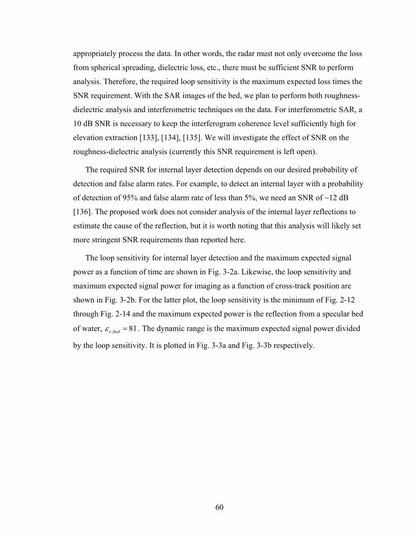
60

appropriately process the data. In other words, the radar must not only overcome the loss

from spherical spreading, dielectric loss, etc., there must be sufficient SNR to perform

analysis. Therefore, the required loop sensitivity is the maximum expected loss times the

SNR requirement. With the SAR images of the bed, we plan to perform both roughness-

dielectric analysis and interferometric techniques on the data. For interferometric SAR, a

10 dB SNR is necessary to keep the interferogram coherence level sufficiently high for

elevation extraction [133], [134], [135]. We will investigate the effect of SNR on the

roughness-dielectric analysis (currently this SNR requirement is left open).

The required SNR for internal layer detection depends on our desired probability of

detection and false alarm rates. For example, to detect an internal layer with a probability

of detection of 95% and false alarm rate of less than 5%, we need an SNR of ~12 dB

[136]. The proposed work does not consider analysis of the internal layer reflections to

estimate the cause of the reflection, but it is worth noting that this analysis will likely set

more stringent SNR requirements than reported here.

The loop sensitivity for internal layer detection and the maximum expected signal

power as a function of time are shown in Fig. 3-2a. Likewise, the loop sensitivity and

maximum expected signal power for imaging as a function of cross-track position are

shown in Fig. 3-2b. For the latter plot, the loop sensitivity is the minimum of Fig. 2-12

through Fig. 2-14 and the maximum expected power is the reflection from a specular bed

of water, 81, =bedrε . The dynamic range is the maximum expected signal power divided

by the loop sensitivity. It is plotted in Fig. 3-3a and Fig. 3-3b respectively.

61

500 1000 1500 2000 2500 3000-240

-220

-200

-180

-160

-140

-120

-100

Range (m)

Pt /

Pr (d

B)

Loop SensitivityMax Power

0 200 400 600 800 1000

-220

-210

-200

-190

-180

-170

-160

-150


Pt /

Pr (d

B)

Loop SensitivityMax Power

Fig. 3-2. a) Loop sensitivity and maximum expected power from internal layer reflections plotted versus

time. b) Loop sensitivity and maximum expected power from basal scattering plotted versus cross-track

dimension (individual test cases are shown as dashed lines in the background).

0 500 1000 1500 2000 2500 3000 350040

45

50

55

60

65

70

75

80

85

Range (m)

Dyn

amic

Ran

ge (d

B)

Dynamic RangeDynamic Range w/ 220 dB Limit

0 200 400 600 800 10000

20

40

60

80

100


Dyn

amic

Ran

ge (d

B)

Dynamic RangeDynamic Range w/ 220 dB Limit

Fig. 3-3. a) Dynamic range plotted versus time. b) Dynamic range plotted versus cross-track dimension.

A further complication arises when pulse compression is used to increase signal-to-

noise ratio. In this case, a long pulse of length pulseτ is generated that simultaneously

engages many layers of the ice sheet. See Fig. 3-4 for an illustration of this. In this

example, the radar must be sensitive to the weak return from layer B while not saturating

when receiving the return from layer A.

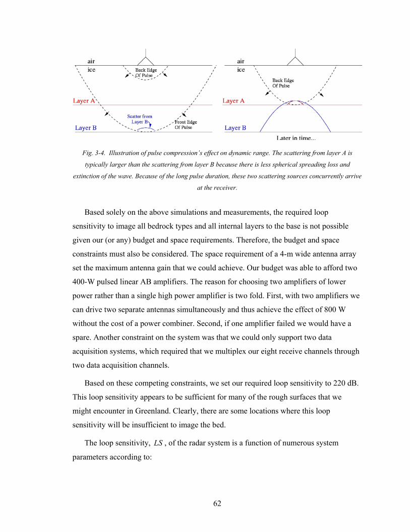
62

Fig. 3-4. Illustration of pulse compression’s effect on dynamic range. The scattering from layer A is

typically larger than the scattering from layer B because there is less spherical spreading loss and

extinction of the wave. Because of the long pulse duration, these two scattering sources concurrently arrive

at the receiver.

Based solely on the above simulations and measurements, the required loop

sensitivity to image all bedrock types and all internal layers to the base is not possible

given our (or any) budget and space requirements. Therefore, the budget and space

constraints must also be considered. The space requirement of a 4-m wide antenna array

set the maximum antenna gain that we could achieve. Our budget was able to afford two

400-W pulsed linear AB amplifiers. The reason for choosing two amplifiers of lower

power rather than a single high power amplifier is two fold. First, with two amplifiers we

can drive two separate antennas simultaneously and thus achieve the effect of 800 W

without the cost of a power combiner. Second, if one amplifier failed we would have a

spare. Another constraint on the system was that we could only support two data

acquisition systems, which required that we multiplex our eight receive channels through

two data acquisition channels.

Based on these competing constraints, we set our required loop sensitivity to 220 dB.

This loop sensitivity appears to be sufficient for many of the rough surfaces that we

might encounter in Greenland. Clearly, there are some locations where this loop

sensitivity will be insufficient to image the bed.

The loop sensitivity, LS , of the radar system is a function of numerous system

parameters according to:

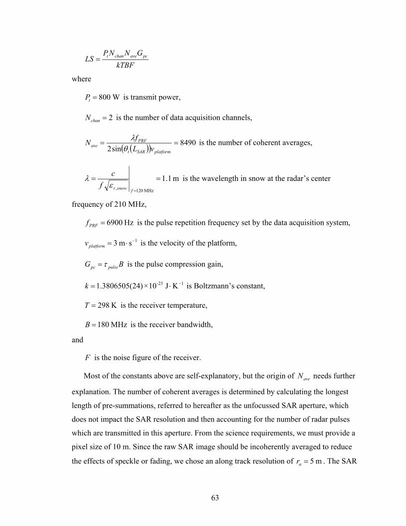
63

kTBFGNNP

LS pcavechant=

where

W800=tP is transmit power,

2=chanN is the number of data acquisition channels,

( )( ) 8490sin2

==platformSARt

PRFave vL

fNθλ is the number of coherent averages,

m1.1MHz120,

===fsnowrf

cε

λ is the wavelength in snow at the radar’s center

frequency of 210 MHz,

Hz6900=PRFf is the pulse repetition frequency set by the data acquisition system,

1sm3 −⋅=platformv is the velocity of the platform,

BG pulsepc τ= is the pulse compression gain,

1-23 KJ10 × 24)1.3806505( −⋅=k is Boltzmann’s constant,

K298=T is the receiver temperature,

MHz180=B is the receiver bandwidth,

and

F is the noise figure of the receiver.

Most of the constants above are self-explanatory, but the origin of aveN needs further

explanation. The number of coherent averages is determined by calculating the longest

length of pre-summations, referred to hereafter as the unfocussed SAR aperture, which

does not impact the SAR resolution and then accounting for the number of radar pulses

which are transmitted in this aperture. From the science requirements, we must provide a

pixel size of 10 m. Since the raw SAR image should be incoherently averaged to reduce

the effects of speckle or fading, we chose an along track resolution of m5=ar . The SAR

64

aperture length, SARL , is defined here as the length at which the beam-pattern of the SAR

places a null in the adjacent pixel (5 m away). This corresponds to a 2λ phase shift across

the aperture from a wave originating from an adjacent pixel (see Fig. 3-5). The half-

beamwidth as defined by the first null is a more complicated function than the simple

geometry shown in Fig. 3-5 due to refraction and we thus define it as ( )at rθ . This SAR

aperture length is then ( )( ) m586sin2

==at

SAR rL

θλ . This SAR aperture length now

becomes the finest unfocussed SAR resolution allowed. Any finer resolution will begin to

destructively cancel the pixel energy that the SAR processing uses. The half-beamwidth

for the unfocussed SAR resolution, as defined by the first null, is ( )SARt Lθ . Using the

same 2λ phase shift criterion, the largest unfocussed SAR aperture is

( )( ) m7.3sin2

==SARt

unfocused LL

θλ . The number of pulses taken in the aperture is

8490==platform

PRFunfocusedave v

fLN .

Fig. 3-5. Demonstration of beamwidth (defined null to null) requirement to achieve an along track

resolution of ar .

65

The two unknowns in the loop sensitivity equation are the pulse compression gain

and the noise figure of the receiver. Since the bandwidth is 180 MHz, we only need to

know the transmit pulse duration to calculate the pulse compression gain. We would like

to maximize the pulse duration subject to the dynamic range requirement. Based on the

analysis described in the following dynamic range discussion, we set the pulse duration to

µs10=pulseτ , which provides a pulse compression gain of dB6.32== BG pulsepc τ . Based

on available technology, we were able to achieve a receiver noise figure of 2 dB (includes

band-pass-filter and limiter insertion losses used to protect the receiver). The loop

sensitivity is then 223 dB. However, the following factors must be considered:

6. 10 µs pulse only transmitted 8 out of 9 pulses (see dynamic range discussion for the

reason for this)

7. Power amplifier has non-flat gain and the average power is 50% of peak power13.

8. Antenna feed network, including the low pass filter and transmit antenna switches

which followed the power amp add 2 dB of loss.

The new loop sensitivity calculation is 218 dB, which is 2 dB short of our desired

loop sensitivity.

The dynamic range is a function of the analog-to-digital converter, compression gain,

number of channels, coherent averages, receiver blanking, transmit waveform, and

thermal noise to quantizer noise ratio. The analog-to-digital converter is a 9-bit converter,

with approximately 8 effective bits [137]. This gives a raw dynamic range of

( ) dB48dB68 ==ADCD .

The compression gain adds

( ) ( ) ( ) ( )pulsepulsepcpc BGD ττ 10101010 log10dB6.82log10log10log10 +=+== .

The two receiver channels add

( ) dB3log10 10 == chanchan ND .

The coherent averages add

13 With predistortion of the transmit pulse, this power loss could have been circumvented. However, our transmit waveform was generated by a DDS which could only produce a simple linear FM chirp.

66

( ) dB3.39log10 10 == aveave ND .

Receiver blanking does not change the dynamic range, but protects the receiver

during transmission. The length of the blanking period is set by the transmit waveform’s

pulse duration pulseτ and the scattering properties of the scene. The thermal noise to

quantizer noise floor ratio must be sufficiently large to allow effective coherent averages

(i.e. dithering) [138]. Essentially, the maximum number of effective coherent averages is

set by this ratio and can be determined by laboratory measurements of the analog-to-

digital converter14. To determine our required maximum number of averages, we

consider two constraints. The first is that we wanted to be able to slow, and even stop, the

platform to allow more coherent averages when an increased SNR was desired. Also,

when calibrating the radar system via loopback tests, we take many averages to determine

the transfer function of the system. To accommodate this functionality, we set the desired

coherent averaging capability to one million averages (2.5 minutes of averaging at a PRF

of 6900 Hz). Based on lab measurements, we set our minimum thermal noise to quantizer

noise floor to dB20=ditherD .

We consider two pulse durations here, =pulseτ µs1 and =pulseτ µs10 :

dB9.92µs11 =−+++=

= ditheravechanpcADCs DDDDDDpulseτµ

dB9.102µs1010 =−+++=

= ditheravechanpcADCs DDDDDDpulseτµ

By adjusting the receiver gain and transmitter pulse width of three different radar

configurations, we found we were able to meet most of the dynamic range and loop

sensitivity requirements. The three configuration settings are given in Table 3-1. The

transmitter transmits 9 different waveforms. The first waveform is 1 µs and the second

through ninth are 10 µs. When the 1 µs waveform is transmitted, the two receivers/data

acquisition channels have different gain settings to cover different regions of the required

dynamic range. The low-gain channel’s gain does not raise the thermal noise floor above

the quantizer noise floor, so its dynamic range is less because of this. Also, dB831 =sD µ

because this transmit waveform is only sent about 10% of the time. Almost 90% of the

14 The digital system employs zero-pi modulation which is essential to taking advantage of dithering.

67

time, the 10 µs waveform is transmitted and both receive channels are being used to

sample at maximum gain. The sixteen combinations possible with the 10 µs waveforms

(8 transmit pulses with 2 receivers) are used to sample each of the possible antenna

configurations (see section 3.4 below for more detail on the antenna network). This

technique of utilizing multiple radar configurations required creating software and

hardware that allowed the radar configuration (e.g. digital attenuator settings, transmit

waveform, etc) to change on a pulse-to-pulse basis.

Table 3-1: Radar Waveforms Configuration Transmit

Waveform

Receiver

Channel

Start

Range

Max.

Loss

Min.

Loss

1 µs low-gain 1 1 150 m 160 dB 90 dB

1 µs high-gain 1 2 1200 m 200 dB 117 dB

10 µs high-gain/SAR 2-9 1 & 2 1700 m 218 dB 116 dB

3.4 ANTENNA NETWORK

Both the transmitter and receiver use an array of elements where each element is a

TEM horn antenna [130], [131]. To ease shipping and manufacturing problems, we chose

the same element type and size for both arrays. The minimum frequency of operation was

determined by the antenna networks’ ability to provide sufficient left/right isolation and

suppression of the nadir (specular) echo while meeting our maximum cross-track array

dimension of 4 m. The isolation and suppression requirement translated to an

approximate footprint size of 500 m (footprint size on the bed defined by the null to null

spacing). A plot of footprint size versus frequency is shown in Fig. 3-6 for a 4-m long

transmit and receive antenna array. Only the outside elements of the transmit array are

used. The reason for this is discussed later. Based on these results, the low frequency was

set to 120 MHz. The footprint is ~700 m, which is larger than desired, but simulations

showed that this still provided 10 dB of nadir suppression.

68

50 100 150 200 250300

400

500

600

700

800

900

1000

Frequency (MHz)

Foot

prin

t (m

)

Fig. 3-6. Footprint of antenna array versus frequency. This assumes that only the outside elements of the

transmit array are used.

Based on data taken in 2004 with the TEM horn antennas, we found that the antenna

element size would need to be ~24 inches on a side to provide sufficient matching at 120

MHz. This meant that we could place eight elements in the array. Because we need the

ability to electronically scan with our array, we cannot simultaneously excite transmit

elements arrayed in the cross-track dimension since this would fix the main lobe of the

transmit array. Therefore, each element of the transmit array must be excited one at a

time. Due to data system limitations, we could not meet our Nyquist sampling rate and

multiplex across both transmit and receive elements (8 receive elements times 8 transmit

elements equals 64 configurations). To solve this problem, we used a sparse transmit

array with two elements, one on each end of the array. This technique produces a cross-

track beam pattern that is approximately half as large, but the side lobe performance is

similar to a single element. An analogous situation arises when a real aperture is

compared to a SAR aperture. The SAR aperture has twice as fine resolution (half the

beamwidth), but the side lobe performance is worse. The reason for this difference is that

both the transmitter and receiver move together which doubles the phase-delay.

To increase our transmit power and gain and to improve the return loss of our

transmit antennas, we arrayed two transmit antennas in the along track direction. This

also allowed for a convenient way to combine the power of our two amplifiers. The TEM

horn elements have significantly better return loss when arrayed in the H-plane rather

69

than fed as single elements. This improvement in return loss is shown in Fig. 3-7 (based

on S-parameter measurements taken at Summit, Greenland).

150 200 250 300-15

-10

-5

0

Frequency (MHz)

Ret

urn

Loss

(dB

)a)

150 200 250 300-15

-10

-5

0

Frequency (MHz)

Ret

urn

Loss

(dB

)

b)

Fig. 3-7. Return loss of a) a single antenna and b) two H-plane arrayed antennas fed simultaneously.

Another technique for improving both the noise figure of the receiver and improving

the matching to the receive elements is to place the low noise amplifier at the input to the

antenna. Any mismatches or “ringing” that occurs between the antenna and the low noise

amplifier settles rapidly because the transmission line connecting the two is very short15.

A DC bias on the RF feed cables is used to power the amplifiers.

The E-plane and H-plane simulations of the antennas at our center frequency are

shown in Fig. 3-8 [95]. A diagram of the antenna network is given in Fig. 3-9.

15 The reverse isolation of the LNA is more than 10 dB which reduces reflections through the LNA to a tolerable level.

70

0 5 10 15 20 25 30-4

-3

-2

-1

0

1

2

3

4

Angle θt (deg)

E-p

lane

Gai

n (d

B)

0 5 10 15 20 25 300

1

2

3

4

5

6

7

8

Angle θt (deg)

H-p

lane

Gai

n (d

B)

Fig. 3-8. Simulated a) E-plane and b) H-plane antenna gain patterns of TEM horn antennas at 210 MHz

(main lobe is at zero degrees and patterns are nearly symmetrical about the main lobe).

Fig. 3-9. Diagram of antenna network configuration.

3.5 BISTATIC RECEIVER

For the bistatic receiver to operate, it must synchronize control and timing signals

with the transmitter. It also needs to provide phase synchronization even when the raw

signal (uncompressed and minimal coherent averages) is 30-50 dB beneath the noise

floor. This is provided through two mechanisms. The first is an IEEE 802.11 wireless

network that provides a link to synchronize the radar control parameters such as pulse

repetition frequency, transmit waveform, position and heading information, etc. The

71

second mechanism provides the timing synchronization (locking the PRF signal and

locking the phase). To do this, both the monostatic transmitter and bistatic receiver are

referenced off an atomic standard, programmable, 10-MHz Rubidium source.

Additionally, the PRF signal is programmable.

The radar control parameters are transported through the network so that each end of

the system (transmitter and bistatic receiver) knows what the transmitted pulse will be,

the PRF, and other pertinent radar settings. After the transmitter begins transmitting, the

bistatic receiver software scans the entire pulse period (equal to the time between pulses)

into a temporary buffer by adjusting the offset of the data capture trigger in reference to

the PRF signal. Once the entire pulse period has been captured, the temporary buffer is

analyzed to find the direct path signal. Then, using high-precision position and heading

information, the range between transmit and receive antennas is found. This range is then

used to offset the location of the direct path signal in the data capture window so that the

bistatic receiver’s PRF signal is aligned with the transmitter’s PRF signal.

Once the PRF signals are locked, the bistatic receiver software begins monitoring the

phase and range bin of the direct path signal. As the radar system moves, new range and

heading information is used to provide accurate range information to the software. Using

this range information and the phase/range-bin of the direct path signal, the Rubidium

source’s frequency is adjusted until the unexpected phase/range-bin drift in the direct

path is zero. After phase locking, the bistatic software allows data to be recorded to disk,

but continues monitoring the direct-path signal and making adjustments to the Rubidium

source as needed.

The phase synchronization requires a very accurate estimate of the range between the

transmit and receive antennas. Using a twentieth of a wavelength as a guideline for

maximum position error, at 300 MHz, the position accuracy should be better than 3 cm.

To provide this quality of ranging information, a differential global positioning system is

used. This provides position information with an error standard deviation of 1 cm in

latitude and longitude, and 2 cm in elevation.

72

3.6 RADAR SPECIFICATIONS

A consolidated list of the radar system specifications is given in Table 3-2. The only

parameter that is not discussed above is the maximum device-to-device reflection level.

This was set to 30 dB to ensure low side lobes due to these reflections.

Table 3-2: Radar System Specifications Specification Value

Frequency Band 120-300 MHz

Loop Sensitivity 220 dB

Dynamic Range 130 dB

Pulse Repetition Frequency 6900 Hz

Transmit Power 800 W

Receiver Noise Figure 2 dB

Maximum Device to

Device Reflection

-30 dB

Number of ADC Channels 2

Transmit Channels 2

Receive Channels 8

Others – Multiple transmit waveforms

– Radar parameters configurable

on a pulse to pulse basis

-- PRF and stable local oscillator

configurable from software for

bistatic operation

3.7 BLOCK DIAGRAMS AND SYSTEM INSTALLATION

This section gives an overview of the radar system and its workings. For an in-depth

description of each component of the radar system, please see [139]. Fig. 3-10 shows the

flow of control and data to and from the various sections of the radar system. To aid in

the discussion, the system is divided into seven sections as shown in Fig. 3-10: computer,

digital, receiver, transmitter, clock synthesizer, power-amp, and multiplexer sections.

Dashed lines indicate the flow of control/timing information and solid lines illustrate

signal flow (whether in analog or quantized form).

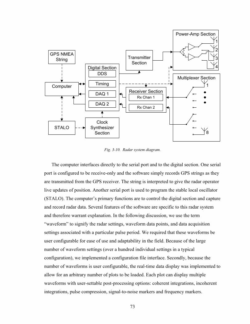
73

TransmitterSection

Clock Synthesizer

Section

ComputerReceiver Section

Rx Chan 1

Rx Chan 2

Multiplexer Section1

8

Power-Amp Section

2

1

3

4Digital SectionDDS

Timing

DAQ 2

DAQ 1

GPS NMEA String

STALO

Fig. 3-10. Radar system diagram.

The computer interfaces directly to the serial port and to the digital section. One serial

port is configured to be receive-only and the software simply records GPS strings as they

are transmitted from the GPS receiver. The string is interpreted to give the radar operator

live updates of position. Another serial port is used to program the stable local oscillator

(STALO). The computer’s primary functions are to control the digital section and capture

and record radar data. Several features of the software are specific to this radar system

and therefore warrant explanation. In the following discussion, we use the term

“waveform” to signify the radar settings, waveform data points, and data acquisition

settings associated with a particular pulse period. We required that these waveforms be

user configurable for ease of use and adaptability in the field. Because of the large

number of waveform settings (over a hundred individual settings in a typical

configuration), we implemented a configuration file interface. Secondly, because the

number of waveforms is user configurable, the real-time data display was implemented to

allow for an arbitrary number of plots to be loaded. Each plot can display multiple

waveforms with user-settable post-processing options: coherent integrations, incoherent

integrations, pulse compression, signal-to-noise markers and frequency markers.

74

Another potential pitfall that the software has to avoid is digital section buffer

overflows. The buffers in the digital section can only hold a single record in memory.

Therefore, the software must upload the data immediately to prevent buffer overflows. To

guarantee the highest level of responsiveness, the data-upload and recording tasks were

each given their own thread. Also, a large first-in-first-out (FIFO) was implemented in

the recording thread to hold many data records at once. In case a write to the hard drive

stalls, the data thread can continue to write to the FIFO. The FIFO also held data for

display to the graphical user interface. Since the real-time display was secondary to data

capture, all post-processing besides coherent integrations is performed inside the

graphical user interface thread.

The digital section is comprised of three parts: timing, DDS, and DAQ. The timing

subsystem not only generates all the timing signals for the DDS and two DAQs, it also

configures the timing backplane for the radar system and generates all the radar control

signals. The DDS generates the linear FM chirp waveforms and its output is connected to

the transmitter section. The two DAQs capture waveforms from each of the respective

receivers in the receiver section. The clocking of samples for both the DDS and DAQs is

from the 720 MHz clock synthesizer.

The clock synthesizer section is shown in Fig. 3-11. The phase locked oscillator is

implemented inside a configurable Silicon Labs part which is loaded on power-up by an

on-board programmable logic device. The signal is then amplified and filtered before

being distributed to each DAQ and the DDS. To minimize channel mismatch, power

dividers with very tight amplitude and phase balance specifications were used.

75

Fig. 3-11. Block diagram of clock synthesizer.

The DDS generates the pulse which is then filtered, amplified, and filtered again by

the transmitter section, shown in Fig. 3-12, before being sent to the power-amp section.

The DDS also generates a calibration tone after the linear FM chirp is generated. The

single-pole double-throw (SPDT) switch is used to pass this calibration signal to the

receiver, bypassing the power-amp section. Thus, the calibration tone passes through the

transmitter and receiver sections, but is slightly outside the band of interest so that it does

not interfere with the signal. The calibration tone is used to verify the phase and

amplitude stability of the radar and to verify that the timing section was not producing

any jitter in the data.

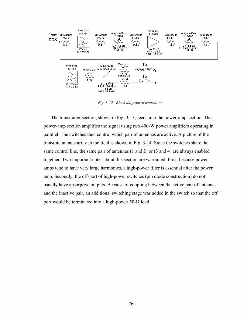
76

Fig. 3-12. Block diagram of transmitter.

The transmitter section, shown in Fig. 3-13, feeds into the power-amp section. The

power-amp section amplifies the signal using two 400-W power amplifiers operating in

parallel. The switches then control which pair of antennas are active. A picture of the

transmit antenna array in the field is shown in Fig. 3-14. Since the switches share the

same control line, the same pair of antennas (1 and 2) or (3 and 4) are always enabled

together. Two important notes about this section are warranted. First, because power

amps tend to have very large harmonics, a high-power filter is essential after the power

amp. Secondly, the off-port of high-power switches (pin diode construction) do not

usually have absorptive outputs. Because of coupling between the active pair of antennas

and the inactive pair, an additional switching stage was added in the switch so that the off

port would be terminated into a high-power 50-Ω load.

77

Fig. 3-13. Block diagram of power-amp section which includes the antenna feed network.

Fig. 3-14. Transmit antenna array with 4 TEM horn antennas. The transmit array really consists of two

pairs of antennas which operate in parallel for improved return loss characteristics.

78

After the signal is transmitted, it scatters off englacial and subglacial features and is

coupled into one of the eight antennas, see Fig. 3-16. The eight antennas are attached to

the multiplexer section of the radar. The block diagram of the multiplexer section is

shown in Fig. 3-15. The band-selection filter and low noise amplifier (LNA) is placed at

the output of the antenna to reduce reflections off the antenna and to improve the noise

figure of the receiver chain. The LNA has a built in limiter to protect the receiver

circuitry. Power to the LNA is supplied from the main radar system via a DC-bias.

Finally, the eight receive channels are multiplexed onto two channels and passed to one

of the two receivers. Similar to the switch in the power amp section, an absorptive SP4T

switch is used to perform the multiplexing operation.

Fig. 3-15. Receiver antenna array with 8 TEM horn antennas. The front-end band pass filter and low noise

amplifier are fastened directly to the antenna connector.

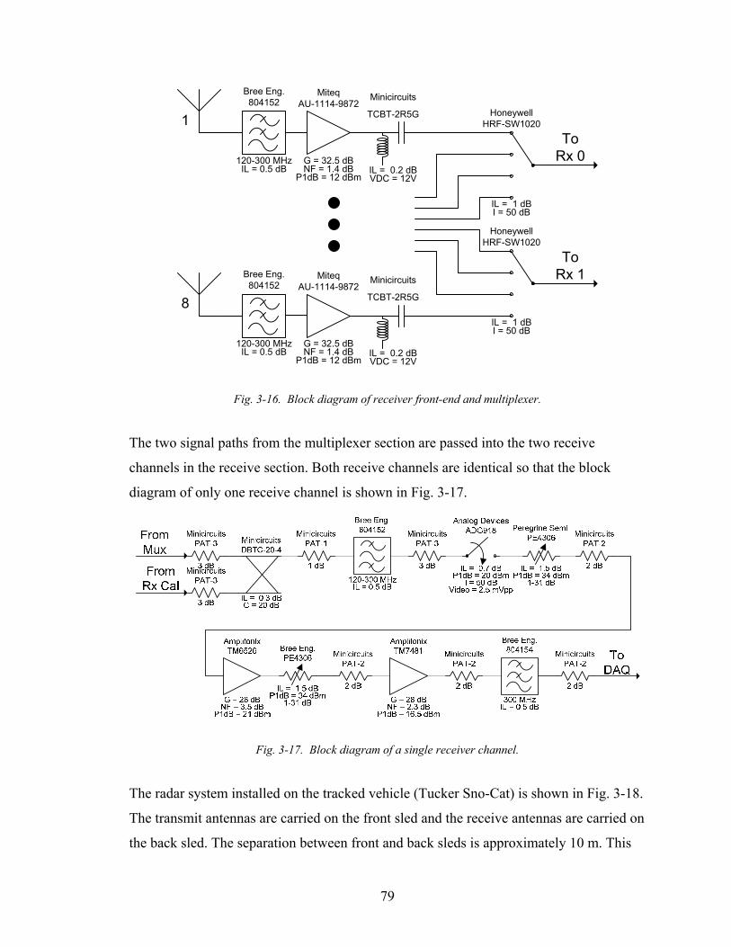
79

Minicircuits

TCBT-2R5G

IL = 0.2 dBVDC = 12V

HoneywellHRF-SW1020

IL = 1 dBI = 50 dB

HoneywellHRF-SW1020

IL = 1 dBI = 50 dB

Minicircuits

TCBT-2R5G

IL = 0.2 dBVDC = 12V

ToRx 0

ToRx 1

Bree Eng.804152

120-300 MHzIL = 0.5 dB

Bree Eng.804152

120-300 MHzIL = 0.5 dB

MiteqAU-1114-9872

G = 32.5 dBNF = 1.4 dB

P1dB = 12 dBm

MiteqAU-1114-9872

G = 32.5 dBNF = 1.4 dB

P1dB = 12 dBm

1

8

Fig. 3-16. Block diagram of receiver front-end and multiplexer.

The two signal paths from the multiplexer section are passed into the two receive

channels in the receive section. Both receive channels are identical so that the block

diagram of only one receive channel is shown in Fig. 3-17.

Fig. 3-17. Block diagram of a single receiver channel.

The radar system installed on the tracked vehicle (Tucker Sno-Cat) is shown in Fig. 3-18.

The transmit antennas are carried on the front sled and the receive antennas are carried on

the back sled. The separation between front and back sleds is approximately 10 m. This

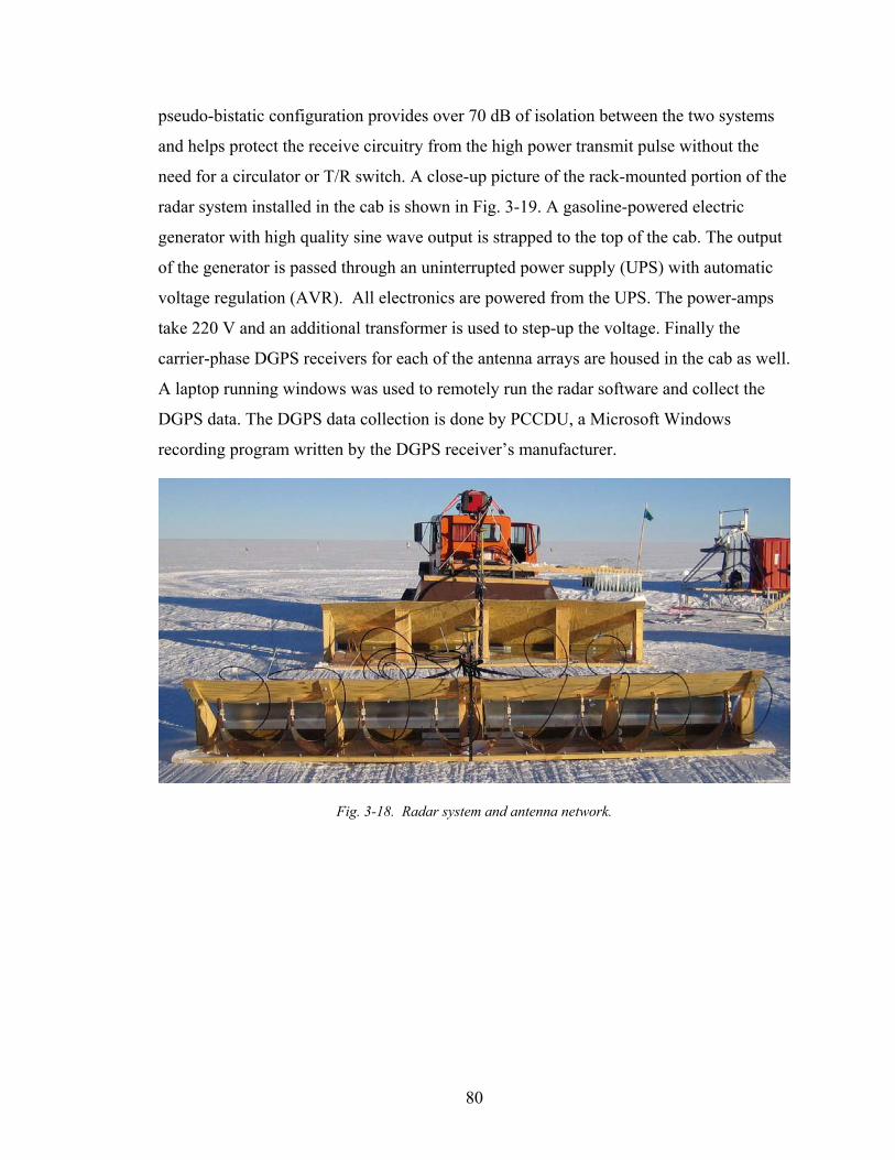
80

pseudo-bistatic configuration provides over 70 dB of isolation between the two systems

and helps protect the receive circuitry from the high power transmit pulse without the

need for a circulator or T/R switch. A close-up picture of the rack-mounted portion of the

radar system installed in the cab is shown in Fig. 3-19. A gasoline-powered electric

generator with high quality sine wave output is strapped to the top of the cab. The output

of the generator is passed through an uninterrupted power supply (UPS) with automatic

voltage regulation (AVR). All electronics are powered from the UPS. The power-amps

take 220 V and an additional transformer is used to step-up the voltage. Finally the

carrier-phase DGPS receivers for each of the antenna arrays are housed in the cab as well.

A laptop running windows was used to remotely run the radar software and collect the

DGPS data. The DGPS data collection is done by PCCDU, a Microsoft Windows

recording program written by the DGPS receiver’s manufacturer.

Fig. 3-18. Radar system and antenna network.

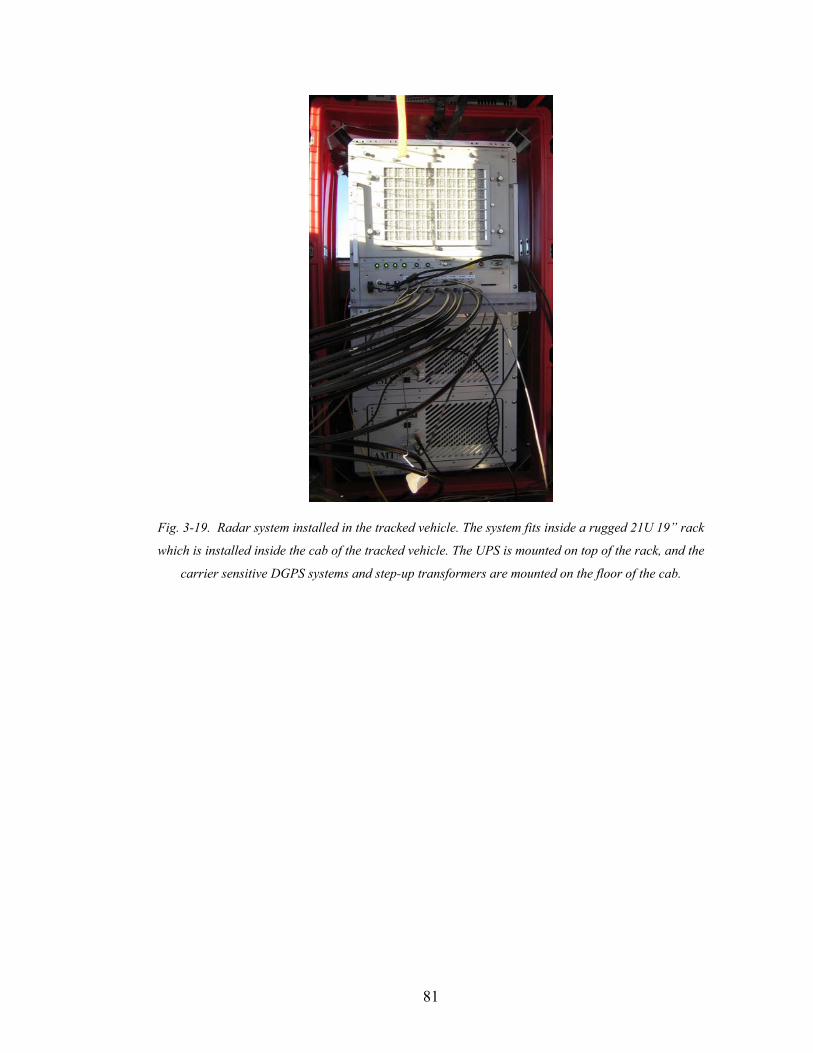
81

Fig. 3-19. Radar system installed in the tracked vehicle. The system fits inside a rugged 21U 19” rack

which is installed inside the cab of the tracked vehicle. The UPS is mounted on top of the rack, and the

carrier sensitive DGPS systems and step-up transformers are mounted on the floor of the cab.

82

Chapter 4: DATA PRECONDITIONING

4.1 INTRODUCTION

This chapter describes the various steps involved in the preparation of the data before

they are passed to the imaging algorithms (f-k migration or SAR processing). These steps

include synchronization of the radar and DGPS data, calibration of the radar data which

is equivalent to a matched filter that removes all cable delays so that all channels have a

common time zero reference, grouping of data into sequences for management purposes,

and finally, the uniform along-track re-sampling of the data for wavenumber domain

filtering.

4.2 TRAJECTORY DATA

To enable image processing and position tagging of data, two Topcon global

positioning system (GPS) units were used to record GPS data. The carrier-phase GPS

data from each unit are recorded by Topcon’s PCCDU Microsoft Windows software. One

unit also outputs a National Marine Electronics Association (NMEA) string to the radar

system computer. This string’s primary purpose is to provide a coarse synchronization

between the radar system and GPS time. This is done by time-stamping the arrival of

each new NMEA string (10 NMEA strings are sent per second). The radar data are

likewise time-stamped by the computer upon arrival. By comparing these time-stamps we

can synchronize the GPS data with the radar data. Due to unknown delays in the serial

port and data acquisition path, this method has limited resolution – probably on the order

of a hundred milliseconds or less. While this delay may be problematic for airborne

applications, it is insignificant considering our slow-moving platform, which is both

unable to change heading or speed rapidly. While a detailed explanation of every step of

the DGPS processing is available in [140], there are several important points and

assumptions that should be pointed out.

83

The primary problem encountered during post-processing the Summit, Greenland

data is that the post-processor provides poor accuracy for substantial portions of the

traverse. Topcon representatives were unable to provide insight and an in-house heuristic

algorithm was generated to alleviate the problem. Parts of the algorithm are automated,

but some portions involve manual and best-guess work. This algorithm for correcting the

data has the important feature that it produces continuous position records. The imaging

algorithms tend to be more tolerant to continuous and slowly varying position errors – as

these types of errors usually cause minor defocusing and shifting of target locations.

Sudden jumps in position errors can result in severe target decorrelation since they do not

correspond to a simple shift of the Doppler centroid. The steps of the process are outlined

here:

Step One…

Instead of passing a single DGPS file to the post-processor, we concatenated the files

into groups of three (the largest size that the post-processor could handle). We then post-

processed the data in overlapping segments. For example, assume we collected five

DGPS files and label these files A, B, C, D, and E. We would then create three

concatenated files: A,B,C, B,C,D, and C,D,E. Each of these files would be post-

processed so that each location would have up to three solutions (see how file C is in all

three concatenated files).

The post-processor provides a solution-type tag for each position: fixed or float. A

location tagged as fixed should be high-precision and a location tagged as float has low-

precision. The problem with passing a single DGPS file, e.g. file C, into the post-

processor was that the output would have many float solution-types. These offending

positions tended to be at the beginning of the file: the DGPS routine is similar to a filter

and suffers from transients. Furthermore, the float solution-types are usually clumped

together and the post-processed position would make a sudden “jump” when the solution

type switched between fixed and float. This jump in position was usually between 0.1 and

2 meters which could cause significant problems to the phase-sensitive imaging

algorithms. The jumps also only occurred at solution-type transitions. In other words, no

jumps occurred in contiguous groups of fixed or float solutions.

84

Step Two…

After post-processing, the multiple results for each location are combined using the

following algorithm:

1. If fixed solution-types are available, the mean of the fixed solutions is taken as the

final result.

2. When a group of float solution-types are encountered, we apply an affine

correction to the group based on the fixed solution-types that surround the group

of bad data. Since the correction method is identical and is the applied

independently along each basis of the coordinate system, we consider only a

single axis. As noted above, a jump in position occurs at the transition from fixed

to float solution-type. The same occurs at the transition from float back to fixed

solution-type. The affine correction is based on this jump. First, we create a first-

order polynomial fit to the last three seconds of good data. This polynomial is

used to predict what the next position should have been. The difference between

this predicted position and the float solution is the starting error of the affine

correction. The same is done at the end of the group of float solutions and this

becomes the ending error. A line is then fit to these two errors and added to the

float solution types.

This method is accurate if the post-processor’s fixed solutions are good and the GPS

errors have low spatiotemporal bandwidth. The latter assumption is what DGPS post-

processing uses to improve relative position accuracy. An example of data before and

after the correction is shown in Fig. 4-1.

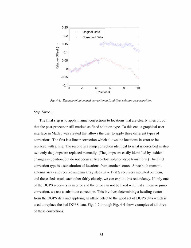
85

0 20 40 60 80 100-0.1

-0.05

0

0.05

0.1

0.15

0.2

0.25

Position #

Rel

ativ

e O

ffset

(m)

Original Data

Corrected Data

Fig. 4-1. Example of automated correction at fixed-float solution-type transition.

Step Three…

The final step is to apply manual corrections to locations that are clearly in error, but

that the post-processor still marked as fixed solution-type. To this end, a graphical user

interface in Matlab was created that allows the user to apply three different types of

corrections. The first is a linear correction which allows the locations-in-error to be

replaced with a line. The second is a jump correction identical to what is described in step

two only the jumps are replaced manually. (The jumps are easily identified by sudden

changes in position, but do not occur at fixed-float solution-type transitions.) The third

correction type is a substitution of locations from another source. Since both transmit

antenna array and receive antenna array sleds have DGPS receivers mounted on them,

and these sleds track each other fairly closely, we can exploit this redundancy. If only one

of the DGPS receivers is in error and the error can not be fixed with just a linear or jump

correction, we use a substitute correction. This involves determining a heading vector

from the DGPS data and applying an affine offset to the good set of DGPS data which is

used to replace the bad DGPS data. Fig. 4-2 through Fig. 4-4 show examples of all three

of these corrections.

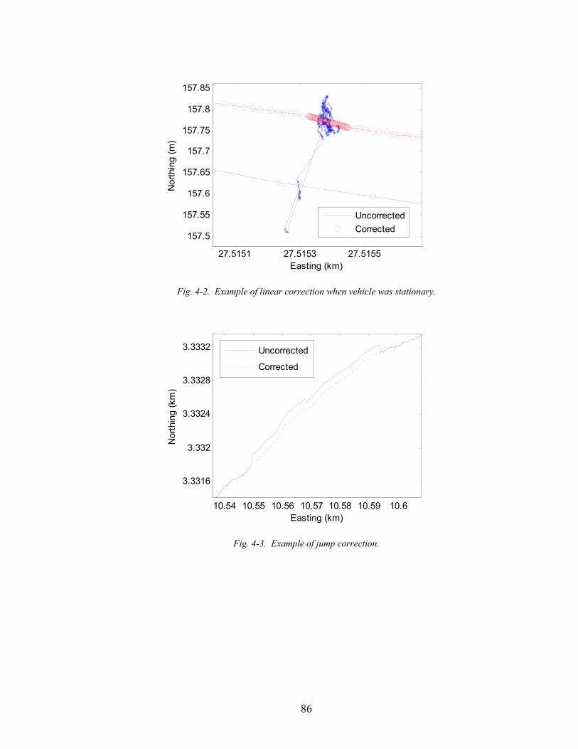
86

27.5151 27.5153 27.5155

157.5

157.55

157.6

157.65

157.7

157.75

157.8

157.85

Easting (km)

Nor

thin

g (m

)

UncorrectedCorrected

Fig. 4-2. Example of linear correction when vehicle was stationary.

10.54 10.55 10.56 10.57 10.58 10.59 10.6

3.3316

3.332

3.3324

3.3328

3.3332

Easting (km)

Nor

thin

g (k

m)

Uncorrected

Corrected

Fig. 4-3. Example of jump correction.

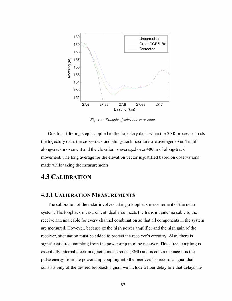
87

27.5 27.55 27.6 27.65 27.7

152

153

154

155

156

157

158

159

160

Easting (km)

Nor

thin

g (m

)

UncorrectedOther DGPS RxCorrected

Fig. 4-4. Example of substitute correction.

One final filtering step is applied to the trajectory data: when the SAR processor loads

the trajectory data, the cross-track and along-track positions are averaged over 4 m of

along-track movement and the elevation is averaged over 400 m of along-track

movement. The long average for the elevation vector is justified based on observations

made while taking the measurements.

4.3 CALIBRATION

4.3.1 CALIBRATION MEASUREMENTS The calibration of the radar involves taking a loopback measurement of the radar

system. The loopback measurement ideally connects the transmit antenna cable to the

receive antenna cable for every channel combination so that all components in the system

are measured. However, because of the high power amplifier and the high gain of the

receiver, attenuation must be added to protect the receiver’s circuitry. Also, there is

significant direct coupling from the power amp into the receiver. This direct coupling is

essentially internal electromagnetic interference (EMI) and is coherent since it is the

pulse energy from the power amp coupling into the receiver. To record a signal that

consists only of the desired loopback signal, we include a fiber delay line that delays the

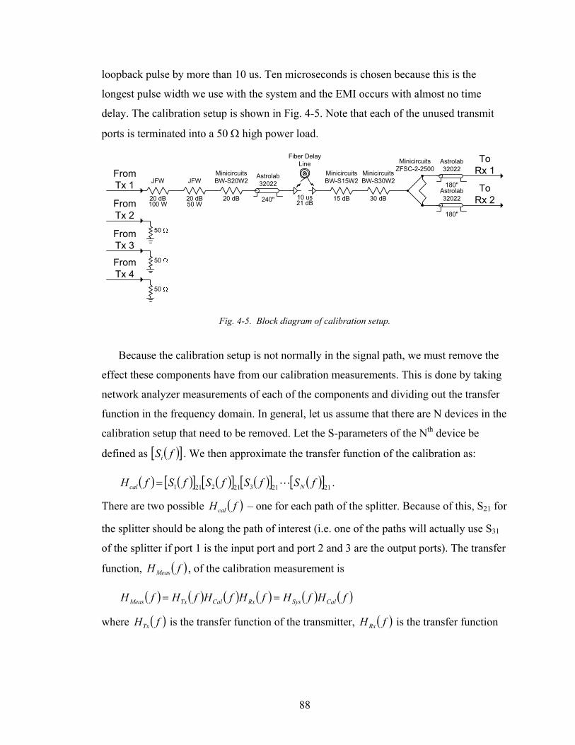
88

loopback pulse by more than 10 us. Ten microseconds is chosen because this is the

longest pulse width we use with the system and the EMI occurs with almost no time

delay. The calibration setup is shown in Fig. 4-5. Note that each of the unused transmit

ports is terminated into a 50 Ω high power load.

JFW

20 dB100 W

MinicircuitsZFSC-2-2500

Fiber DelayLine

10 us21 dB

ToRx 1

ToRx 2

FromTx 1

FromTx 2

FromTx 3

FromTx 4

50

50

50

JFW

20 dB50 W

Astrolab32022

240"

Astrolab32022

180"Astrolab32022

180"

MinicircuitsBW-S20W2

20 dB


15 dB


30 dB

Fig. 4-5. Block diagram of calibration setup.

Because the calibration setup is not normally in the signal path, we must remove the

effect these components have from our calibration measurements. This is done by taking

network analyzer measurements of each of the components and dividing out the transfer

function in the frequency domain. In general, let us assume that there are N devices in the

calibration setup that need to be removed. Let the S-parameters of the Nth device be

defined as ( )[ ]fSi . We then approximate the transfer function of the calibration as:

( ) ( )[ ] ( )[ ] ( )[ ] ( )[ ]21213212211 fSfSfSfSfH Ncal L= .

There are two possible ( )fHcal – one for each path of the splitter. Because of this, S21 for

the splitter should be along the path of interest (i.e. one of the paths will actually use S31

of the splitter if port 1 is the input port and port 2 and 3 are the output ports). The transfer

function, ( )fHMeas , of the calibration measurement is

( ) ( ) ( ) ( ) ( ) ( )fHfHfHfHfHfH CalSysRxCalTxMeas ==

where ( )fHTx is the transfer function of the transmitter, ( )fHRx is the transfer function

89

of the receiver, and ( ) ( ) ( )fHfHfH RxTxSys = is the desired transfer function. Solving for

( )fHSys we find

( ) ( )( )fH

fHfHCal

MeasSys =

This is an appropriate technique when the following is satisfied: 1) the signal-to-noise

ratio (SNR) is very large at all frequencies, and 2) inter-device reflections in the

calibration setup are insignificant. When measuring the calibration setup with the

network analyzer, the setup is broken in to multiple low-attenuation sections and

averaging is used to ensure a large SNR. Furthermore, the return loss of the attenuators

used in the calibration is very high, >40 dB, at our low frequencies of operation.

The radar system captures ( )fHMeas indirectly by capturing a discrete time-domain

signal, ( )nhSys . The discrete Fourier transform is used to find a discrete version of

( )fHMeas . The frequency samples of ( )fHMeas do not necessarily line up with the

frequency samples of the device measurements, ( )[ ]21fSi . Since the amplitude of each

( )[ ]21fSi is a slowly varying function of frequency and the phases are nearly linear, we

use linear interpolation to find the values of ( )[ ]21fSi at the frequency points ( )fHMeas is

known at. Also, because of hardware limitations the frequency range covered by each

( )[ ]21fSi does not cover the same frequency range as ( )fHMeas which is a baseband

signal. Because ( )[ ]21fSi is evaluated at all frequencies where significant energy is

present in the system, we only need to make sure that there are no sudden transitions in

its spectrum. In other words, we can not just zero-pad ( )[ ]21fSi . The method we use is to

linearly extrapolate the phase and to extrapolate the amplitude with the nearest neighbor

method. Fig. 4-6 shows ( )[ ]21fSi before and after extrapolation. We also force conjugate

symmetry as shown in the figure.

90

0 100 200 300 400 500 600 700-40.2

-40.1

-40

Frequency (MHz)

S21

(dB

)

0 100 200 300 400 500 600 700-400

-200

0

200

400

Frequency (MHz)

angl

e(S

21) (

deg)

Original

Extrapolated

Fig. 4-6. ( )[ ]21fSi before and after extrapolation.

Since there are two transmit antennas active at any given time and each signal path

has its own phase and amplitude distortions we measure both of these paths. In the actual

measurements these two paths are essentially added together in phase (all targets of

interest are in the main lobe of the two-element array). Therefore the reference function is

simply the summation of these two paths as well.

To ensure a high SNR for the calibration measurements, 1000000+ pulses are

coherently averaged. After averaging and deconvolution as described above, we truncate

the end of the time-domain record to remove unwanted time-domain noise as well as

circular convolution effects from the deconvolution step. The signal is then down-

converted to baseband, ( ) ( )( )ntfjnh cSys π2exp − where ( )nt is the time-axis. The next step

is to normalize the baseband signal to create a reference function for matched filter pulse

compression: ( ) ( ) ( )( )( ) ( )( ) 2

22exp

2exp

ntfjnh

ntfjnhnh

cSys

cSysefR

π

π

−

−= . The normalization ensures that system

effects are removed. For example, a power level of 0.01 at the output of the properly

normalized matched filter implies that the signal has undergone 20 dB of loss. Because of

91

the small signal levels expected (< -200 dB) and rounding errors resulting from limited

computer precision, we add in a 100 dB offset during the normalization process. This

keeps the signal levels closer to the center of the double precision range. Finally, this

process is repeated for every channel combination so that each channel has its own

reference function and any channel phase or amplitude mismatch can be removed.

4.3.2 PRE-PROCESSING AND MATCHED FILTER Before the matched filter is applied to the radar data, several steps are applied for

memory and speed reasons. The first is pre-summing which is the process of averaging

adjacent records and then decimating the result. This process is shown in Fig. 4-7 for

clarity. Essentially, this is equivalent to time-domain convolution with a boxcar window

and decimation at a rate equal to the width of the boxcar window. The reason for the pre-

summing is to reduce the amount of data that must be dealt with in the later and more

time-consuming image processing.

Fig. 4-7. Example of pre-summing as along-track filtering and decimation when 4=xM .

After pre-summing, the data are down-converted to complex baseband via time

domain multiplication with ( )( )ntfj cπ2exp − as shown in Fig. 4-8. Note that the effective

frequency axis is shifted: the imaging algorithms use the shifted frequency axis when

applying phase shifts.

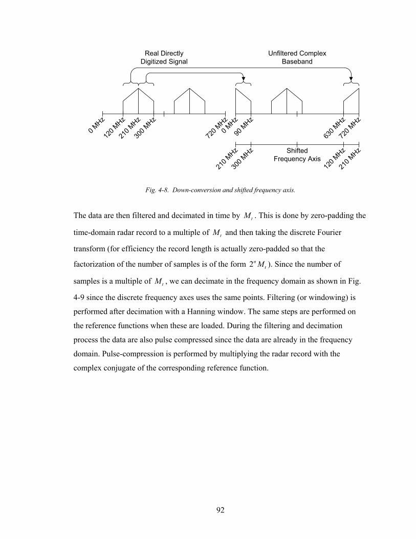
92

0 MHz

720 M

Hz

300 M

Hz

120 M

Hz

210 M

Hz

0 MHz

720 M

Hz

90 M

Hz

630 M

Hz

300 M

Hz

120 M

Hz

210 M

Hz

210 M

HzShifted Frequency Axis

Unfiltered Complex Baseband

Real Directly Digitized Signal

Fig. 4-8. Down-conversion and shifted frequency axis.

The data are then filtered and decimated in time by tM . This is done by zero-padding the

time-domain radar record to a multiple of tM and then taking the discrete Fourier

transform (for efficiency the record length is actually zero-padded so that the

factorization of the number of samples is of the form tn M2 ). Since the number of

samples is a multiple of tM , we can decimate in the frequency domain as shown in Fig.

4-9 since the discrete frequency axes uses the same points. Filtering (or windowing) is

performed after decimation with a Hanning window. The same steps are performed on

the reference functions when these are loaded. During the filtering and decimation

process the data are also pulse compressed since the data are already in the frequency

domain. Pulse-compression is performed by multiplying the radar record with the

complex conjugate of the corresponding reference function.

93

0 MHz

90 M

Hz

180 M

Hz

0 MHz

720 M

Hz

360 M

Hz

Fig. 4-9. Decimation applied in the frequency domain where 4=tM .

4.4 DATA INDEXING METHOD: SEQUENCES

To ease data management and to allow the image processing algorithms to be

independent of this particular set of radar data, a data indexing scheme is laid on top of

the actual data. This indexing scheme takes care of loading the radar and trajectory data

and also identifies sequences of similar data. For example, in a given day, we have to

move the radar platform to the scene of interest, take a few swaths of data, and then

return to the camp. When applying f-k migration and SAR processing, we want to be able

to identify turns, straight segments, and the transits to and from the scene. To this end, a

graphical user interface (GUI) was created in Matlab to identify and tag groups of data.

The GUI is shown in Fig. 4-10. We define a sequence to be a contiguous group of data

where all the data in the group should have the same processing applied to it. A set of

functions, e.g. sequenceOpen, sequenceLoad, sequenceGet, etc. allow generic access to

the data and also provide transparent synchronization to the trajectory data.

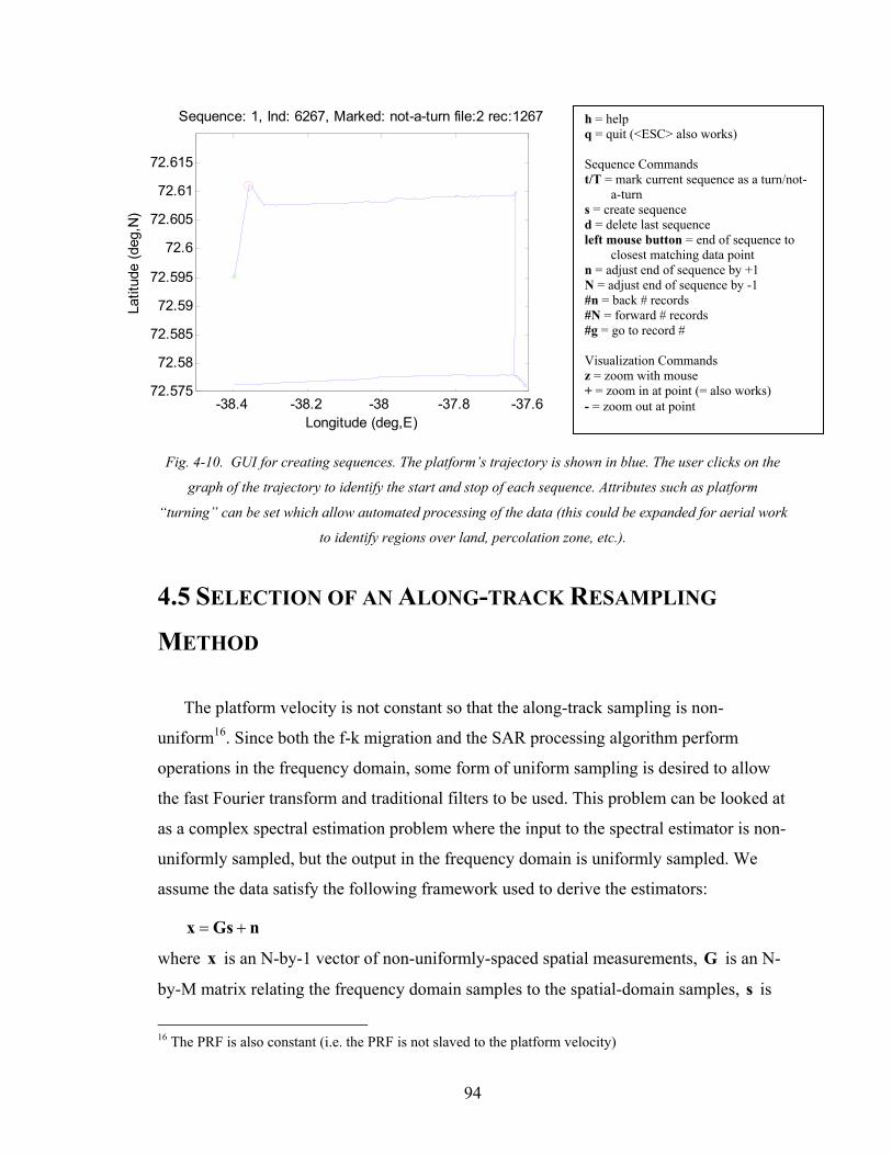
94

-38.4 -38.2 -38 -37.8 -37.672.575

72.58

72.585

72.59

72.595

72.6

72.605

72.61

72.615

Longitude (deg,E)

Latit

ude

(deg

,N)

Sequence: 1, Ind: 6267, Marked: not-a-turn file:2 rec:1267

Fig. 4-10. GUI for creating sequences. The platform’s trajectory is shown in blue. The user clicks on the

graph of the trajectory to identify the start and stop of each sequence. Attributes such as platform

“turning” can be set which allow automated processing of the data (this could be expanded for aerial work

to identify regions over land, percolation zone, etc.).

4.5 SELECTION OF AN ALONG-TRACK RESAMPLING

METHOD

The platform velocity is not constant so that the along-track sampling is non-

uniform16. Since both the f-k migration and the SAR processing algorithm perform

operations in the frequency domain, some form of uniform sampling is desired to allow

the fast Fourier transform and traditional filters to be used. This problem can be looked at

as a complex spectral estimation problem where the input to the spectral estimator is non-

uniformly sampled, but the output in the frequency domain is uniformly sampled. We

assume the data satisfy the following framework used to derive the estimators:

nGsx +=

where x is an N-by-1 vector of non-uniformly-spaced spatial measurements, G is an N-

by-M matrix relating the frequency domain samples to the spatial-domain samples, s is

16 The PRF is also constant (i.e. the PRF is not slaved to the platform velocity)

h = help q = quit (<ESC> also works) Sequence Commands t/T = mark current sequence as a turn/not-

a-turn s = create sequence d = delete last sequence left mouse button = end of sequence to

closest matching data point n = adjust end of sequence by +1 N = adjust end of sequence by -1 #n = back # records #N = forward # records #g = go to record # Visualization Commands z = zoom with mouse + = zoom in at point (= also works) - = zoom out at point

95

an M-by-1 random vector of uniformly-spaced frequency samples with cross-correlation

matrix Hs E ss=Σ , and n is an N-by-1 random vector of time-domain zero-mean

additive Gaussian noise with cross-correlation matrix Hn E nn=Σ . All vectors and

matrices are complex. The signal and noise variances (i.e. diagonal elements of sΣ and

nΣ ) are denoted 21,sσ , through 2

,Msσ and 21,nσ through 2

, Nnσ . The signal and noise are

assumed to be independent of each other. The matrix, G , is given by:

( )TjxkG exp=

where x is the N-by-1 vector of spatial positions and k is the M-by-1 vector of spatial

frequency points. For uniformly sampled space and frequency data where N = M, G is

the traditional inverse discrete Fourier transform matrix.

Three different methods are derived in the following subsections. This is followed by

a description of the simulation setup and a comparison between each method using

simulated data.

4.5.1 MATCHED ESTIMATOR The matched filter estimator maximizes the SNR of a particular estimate. It does not

consider the correlation of other frequencies with the frequency of interest. With

uniformly sampled spatial data, the frequencies are orthogonal because G is a unitary

matrix. Orthogonal in this context means that the Euclidean inner product between the

space-domain representations of two frequencies is zero. Therefore, there is no need to

consider correlation from other frequencies. With nonuniformly sampled spatial data, the

frequencies are not necessarily orthogonal since G is not necessarily unitary. Therefore,

this correlation limits the performance of the matched filter.

We start by considering the estimate of a single frequency component, xlHmMFms ,ˆ =

where mMF ,l is an N-by-1 vector containing the filter coefficients (note that we have

implicitly forced the estimator to be linear). We define the matched filter to be mMF ,l such

96

that the SNR,

2

,

2

:,,

nl

sGlH

mMF

mmH

mMFE , is maximized. Since we would like the output to equal

ms when there is zero noise and zero interference from other frequencies ( 0=ks when

mk ≠ ), we enforce the constraint17 that 12,:,, =msm

HmMF σGl . The optimization equation is

now mMFnH

mMFH

mMFmsm

HmMFmsm

HmMF

E ,,1

2

,1 2

,:,,2,:,,

minmin llnlGlGl

Σ=== σσ

. This is a constrained optimization

problem that can be solved using the Lagrangian multiplier method. The Lagrangian is

( )12,:,,,, −+Σ msm

HmMFmMFn

HmMF σλ Glll . Taking the derivative of the Lagrangian with respect

to HmMF ,l , we find that the stationary point satisfies 02

,:,, =+Σ msmmMFn σλGl . Because the

optimization function is quadratic and positive, its stationary point must be a minimum.

Solving we get 2,:,

1, msmnmMF σλ Gl −Σ−= . To find λ , we enforce the constraint,

12,:,

1:,,:, =Σ−= −

msmnHmmMF

Hm σλ GGlG , which gives 2

,:,1

:,

1

msmnHm σ

λGG −Σ−

= . Therefore, the

matched filter is

2,:,

1:,

:,1

,msmn

Hm

mnmMF σGG

Gl −

−

ΣΣ

= .

When the noise is independent and identically distributed, nΣ is the identity matrix and

the matched filter simplifies to

2,

2:,

:,,

msm

mmMF

σG

Gl = .

The matched filter for this special case contains no matrix inverses and its computational

complexity is O(N2) since it involves a simple matrix multiply.

4.5.2 LINEAR MINIMUM MEAN SQUARED ERROR ESTIMATOR As the name indicates, the minimum mean squared error (MMSE) estimator

minimizes the mean squared error. As with the matched filter, we force the estimator to

17 This constraint has no effect on the SNR and is essentially a scaling factor that cancels out.

97

be a linear operator18. We again start by considering the estimation of just the mth

frequency component, xlHmMFms ,ˆ = . We define the optimization problem to be

2ˆmin,

mm ssEmMF

−=l

. Inserting the filter into the optimization equation gives:

( ) 2

, mH

mMF sE −+ nGsl

( )( ) ( )( ) HmmMF

HHHm

HmMF ssE −+−+= ,, lnGsnGsl

( )( ) ( ) ( ) 2,,,, m

Hm

HmMFmmMF

HHHmMF

HHHHmMF sssE ++−+−++= nGsllnGslnGsnGsl

Taking the derivative with respect to HmMF ,l , we find that the stationary point satisfies

( )( ) ( ) 0, =+−++ HmmMF

HHH sE nGslnGsnGs .

Now solving for mMF ,l we find

( )( ) ( ) 0, =+−++ HmmMF

HHH sE nGslnGsnGs

( ) 0, =−−+++⇔ Hm

HmmMF

HHHHHH sEsEEEEE nsGlnnGnssnGGssG

( ) 0, =Σ−Σ+Σ⇔ ssmMFnH

s kGlGG

( ) ssnH

smMF kΣΣ+Σ=⇔

− GGGl 1, ,

where we have used the independence of s and n . As with the matched filter, the

optimization function is quadratic and positive and therefore its stationary point must be a

minimum.

Although the filter coefficients only need to be found once, the matrix inversion is

O(N3). Once the filter coefficients are found, applying the filter involves a matrix

multiplication which has computational complexity of O(N2). This method requires the

most knowledge about the signal’s statistics and also has the highest computational

burden.

18 For AWGN, the linear estimator is also the overall optimal estimator.

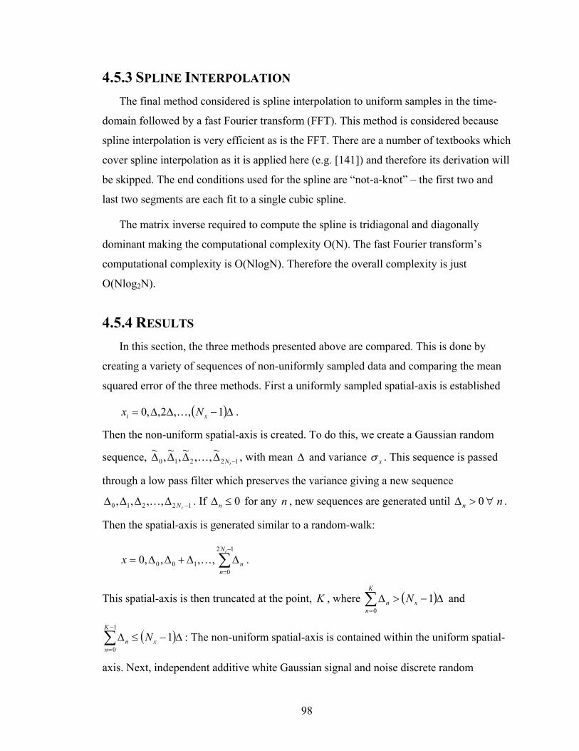
98

4.5.3 SPLINE INTERPOLATION The final method considered is spline interpolation to uniform samples in the time-

domain followed by a fast Fourier transform (FFT). This method is considered because

spline interpolation is very efficient as is the FFT. There are a number of textbooks which

cover spline interpolation as it is applied here (e.g. [141]) and therefore its derivation will

be skipped. The end conditions used for the spline are “not-a-knot” – the first two and

last two segments are each fit to a single cubic spline.

The matrix inverse required to compute the spline is tridiagonal and diagonally

dominant making the computational complexity O(N). The fast Fourier transform’s

computational complexity is O(NlogN). Therefore the overall complexity is just

O(Nlog2N).

4.5.4 RESULTS In this section, the three methods presented above are compared. This is done by

creating a variety of sequences of non-uniformly sampled data and comparing the mean

squared error of the three methods. First a uniformly sampled spatial-axis is established

( )∆−∆∆= 1,,2,,0 xi Nx K .

Then the non-uniform spatial-axis is created. To do this, we create a Gaussian random

sequence, 12210~,,~,~,~

−∆∆∆∆tNK , with mean ∆ and variance xσ . This sequence is passed

through a low pass filter which preserves the variance giving a new sequence

12210 ,,,, −∆∆∆∆tNK . If 0≤∆n for any n , new sequences are generated until nn ∀>∆ 0 .

Then the spatial-axis is generated similar to a random-walk:

∑−

=

∆∆+∆∆=12

0100 ,,,,0

tN

nnx K .

This spatial-axis is then truncated at the point, K , where ( )∆−>∆∑=

10

x

K

nn N and

( )∆−≤∆∑−

=

11

0x

K

nn N : The non-uniform spatial-axis is contained within the uniform spatial-

axis. Next, independent additive white Gaussian signal and noise discrete random

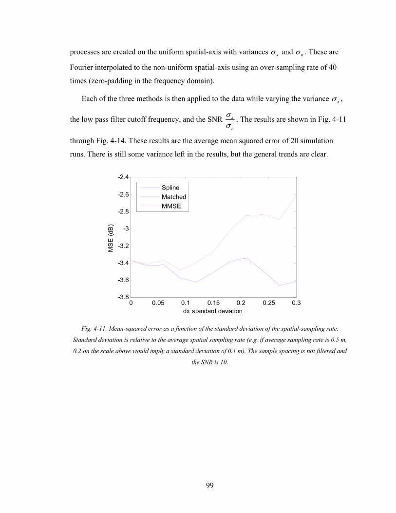
99

processes are created on the uniform spatial-axis with variances sσ and nσ . These are

Fourier interpolated to the non-uniform spatial-axis using an over-sampling rate of 40

times (zero-padding in the frequency domain).

Each of the three methods is then applied to the data while varying the variance xσ ,

the low pass filter cutoff frequency, and the SNR n

s

σσ . The results are shown in Fig. 4-11

through Fig. 4-14. These results are the average mean squared error of 20 simulation

runs. There is still some variance left in the results, but the general trends are clear.

0 0.05 0.1 0.15 0.2 0.25 0.3-3.8

-3.6

-3.4

-3.2

-3

-2.8

-2.6

-2.4

dx standard deviation

MS

E (d

B)

SplineMatchedMMSE

Fig. 4-11. Mean-squared error as a function of the standard deviation of the spatial-sampling rate.

Standard deviation is relative to the average spatial sampling rate (e.g. if average sampling rate is 0.5 m,

0.2 on the scale above would imply a standard deviation of 0.1 m). The sample spacing is not filtered and

the SNR is 10.

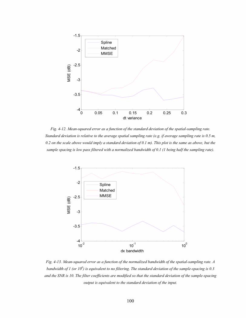
100

0 0.05 0.1 0.15 0.2 0.25 0.3-4

-3.5

-3

-2.5

-2

-1.5

dt variance

MS

E (d

B)

SplineMatchedMMSE

Fig. 4-12. Mean-squared error as a function of the standard deviation of the spatial-sampling rate.

Standard deviation is relative to the average spatial sampling rate (e.g. if average sampling rate is 0.5 m,

0.2 on the scale above would imply a standard deviation of 0.1 m). This plot is the same as above, but the

sample spacing is low pass filtered with a normalized bandwidth of 0.1 (1 being half the sampling rate).

10-2 10-1 100-4

-3.5

-3

-2.5

-2

-1.5

dx bandwidth

MS

E (d

B)

SplineMatchedMMSE

Fig. 4-13. Mean-squared error as a function of the normalized bandwidth of the spatial-sampling rate. A

bandwidth of 1 (or 100) is equivalent to no filtering. The standard deviation of the sample-spacing is 0.3

and the SNR is 10. The filter coefficients are modified so that the standard deviation of the sample-spacing

output is equivalent to the standard deviation of the input.

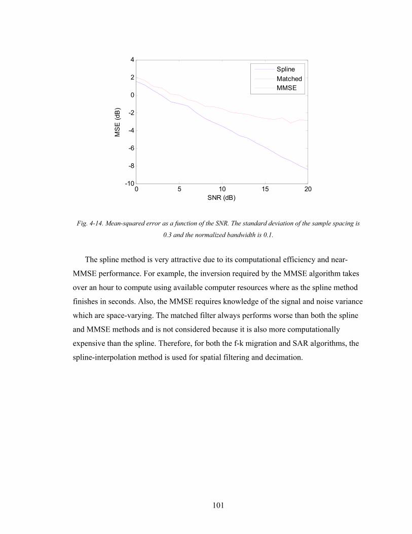
101

0 5 10 15 20-10

-8

-6

-4

-2

0

2

4

SNR (dB)

MS

E (d

B)

SplineMatchedMMSE

Fig. 4-14. Mean-squared error as a function of the SNR. The standard deviation of the sample spacing is

0.3 and the normalized bandwidth is 0.1.

The spline method is very attractive due to its computational efficiency and near-

MMSE performance. For example, the inversion required by the MMSE algorithm takes

over an hour to compute using available computer resources where as the spline method

finishes in seconds. Also, the MMSE requires knowledge of the signal and noise variance

which are space-varying. The matched filter always performs worse than both the spline

and MMSE methods and is not considered because it is also more computationally

expensive than the spline. Therefore, for both the f-k migration and SAR algorithms, the

spline-interpolation method is used for spatial filtering and decimation.

102

Chapter 5: FREQUENCY-WAVENUMBER MIGRATION

5.1 CONCEPT

Frequency-wavenumber migration (f-k migration) as applied here is a synthetic

aperture radar (SAR) algorithm which provides fine along-track resolution of scattering

from the nadir direction. Using a simple detector, ice thickness and bed elevation data

products are garnered from this scattering information. These data products satisfy the

altimetry information needed by the side-looking SAR to generate the system geometry.

The reason f-k migration is used is that it is much more efficient than the side-looking

SAR algorithm described in the next chapter. This is primarily because convolution-like

operations applied in the space-time domain are replaced by multiplication operations in

the frequency-wavenumber domain. In fact, f-k migration is the frequency-wavenumber

domain equivalent of space-time synthetic aperture radar [141], [143]. The algorithm

includes spherical wavefront curvature (i.e. exact range migration) in addition to ordinary

phase correction. Another very useful property of the algorithm is that it efficiently

computes the frequency-wavenumber filter coefficients for layered media19. The

approach taken here for ice sounding is similar to Leuschen et al.’s work with the CoRDS

system used to sound ice in Greenland [125].

To use the multi-dimensional FFT required for f-k migration, the data must be

uniformly spaced in both the time and space domains. The radar provides uniform

sampling in time and the required spatial re-sampling is described in section 4.5. The FFT

also requires the spatial data be taken along a line. However, no motion compensation is

performed before the algorithm. The reason for this is that cross-track motion has

virtually no effect on the focusing of nadir targets. Elevation motion does have an effect,

but the surface slope is very small and nearly constant at the location the measurements

were made as shown in Fig. 5-1. Slopes are about 0.1% or 1 m elevation change for every

1000 m of along-track movement. A constant gradient in the elevation causes a shift in 19 Refraction and velocity changes are incorporated, but the effect of reflection and transmission at interfaces is ignored.

103

the doppler centroid which results in a rotation of the migrated image and degradation in

signal-power for non-isotropic scatterers. Since the shift is so small in this case, signal

loss can be ignored. The rotation is equal to the slope: for 3000 m of ice this results in a 3

m along-track shift in position. This is less than the along-track resolution of the final

image product.

Fig. 5-1. Surface elevation derived from the DGPS measurements taken while collecting the radar data.

Surface is interpolated from discrete DGPS measurements (blue lines) using linear Delaunay triangulation.

To explain the f-k migration algorithm, an analogy restricted to a single dimension is

helpful. Suppose that a plane-wave is traveling in the positive x-direction so that

λπ2

2−== xkk . Since the direction of the wave is set, the wave can be completely

described by its frequency response. Consider a receiver at the origin as shown in Fig.

5-2.

0 x( )ts0 ( )tsx

Fig. 5-2. Spatial shift in one dimension.

Let ( )ts0 denote the signal recorded by the receiver. To determine the signal recorded by

a receiver at position x on the x-axis, ( )tsx , we only need to add a delay of vx so that

104

( )

−=

vxtstsx 0 where v is the velocity of the wave in the medium. In the frequency

domain, using the time-shift property, this corresponds to

( ) ( )

−=

vxfjfSfS x π2exp0

( )

−= x

vfjfS π2exp0

( ) ( )xjkfS xexp0= .

Therefore to determine the frequency response at a position x, we need to multiply

( )fS x with ( )xjkxexp . In the general case, 2222

2zyx kkk ++==

λπk . From the

assumptions we have 0== zy kk and the wave is traveling in the positive direction so

that λπ2

−=xk . To determine the value at zero-time from the frequency domain

response (this will be needed later) we sum all the frequency components together,

( ) ( ) ( ) ( )∫∫∞

∞−

∞

∞−

=⋅= dffSdffjfSs xxx 02exp0 π .

Or if the signal is discrete and of finite length N we have

( ) ( ) ( ) ( )∑∑−

=

−

=

=⋅=1

0

1

00

102exp10N

nx

N

nxx nS

NnfjnS

Ns π .

If the plane-wave is allowed to travel in three dimensions, there are three free

variables xk , yk , and zk but only one constraint equation. However, if the x and y

domain are sampled, this information can be used to determine xk and yk . This leaves

only zk which can be solved as

2222

yxz kkk −−

±=λπ .

105

Assuming that the waves are coming from the negative z direction and substituting in

frequency for wavelength this becomes

( ) 2222,, yxyxz kk

vfkkfk −−

−=π .

Now consider a two dimensional mesh of space-time data collected on the surface of

the ice sheet (e.g. by using a synthetic aperture approach). Let the z-axis be normal to the

surface and point out of the ice. The signal, ( )yxtS ,,0 , at each receiver is a function of

time and the receiver’s position. Also, since all scatterers are located in the ice, k will

always have a positive z component. These data can be transformed to the frequency-

wavenumber domain through a three-dimensional FFT. Each output element of the

three-dimensional FFT is associated with a particular f , xk , and yk given by20:

∆−

∆−

∆+−

∆−

∆−

∆∆+=

ttt

t

t

t

t

t

ttc

NNNff 1,2,...,

21

,2

,2

1,,2,1,0 K ,

∆−

∆−

∆+−

∆−

∆−

∆∆=

xxx

x

x

x

x

x

xxx

NNNk 1,2,...,2

1,2

,2

1,,2,1,02 Kπ ,

∆−

∆−

∆+−

∆−

∆−

∆∆=

yyy

y

y

y

y

y

yyy

NNNk 1,2,...,

21

,2

,2

1,,2,1,02 Kπ ,

where t∆ , x∆ , and y∆ are the spacings in the original space-time domain and tN , xN ,

and yN are the number of samples in each dimension. The space-time data are assumed

to be in the complex baseband form for representing a bandpass signal with a center

frequency of cf . To predict the signal that would have been measured if the mesh of

receivers were moved 1 m in the negative z-direction from their original position, we

solve for zk and then apply a phase shift

( ) ( ) ( )( )1,,exp,,,, 0m1 −⋅=− yxzyxyx kkfjkkkfSkkfS .

20 Assumes an even number of samples (odd number of samples requires the usual simple perturbation).

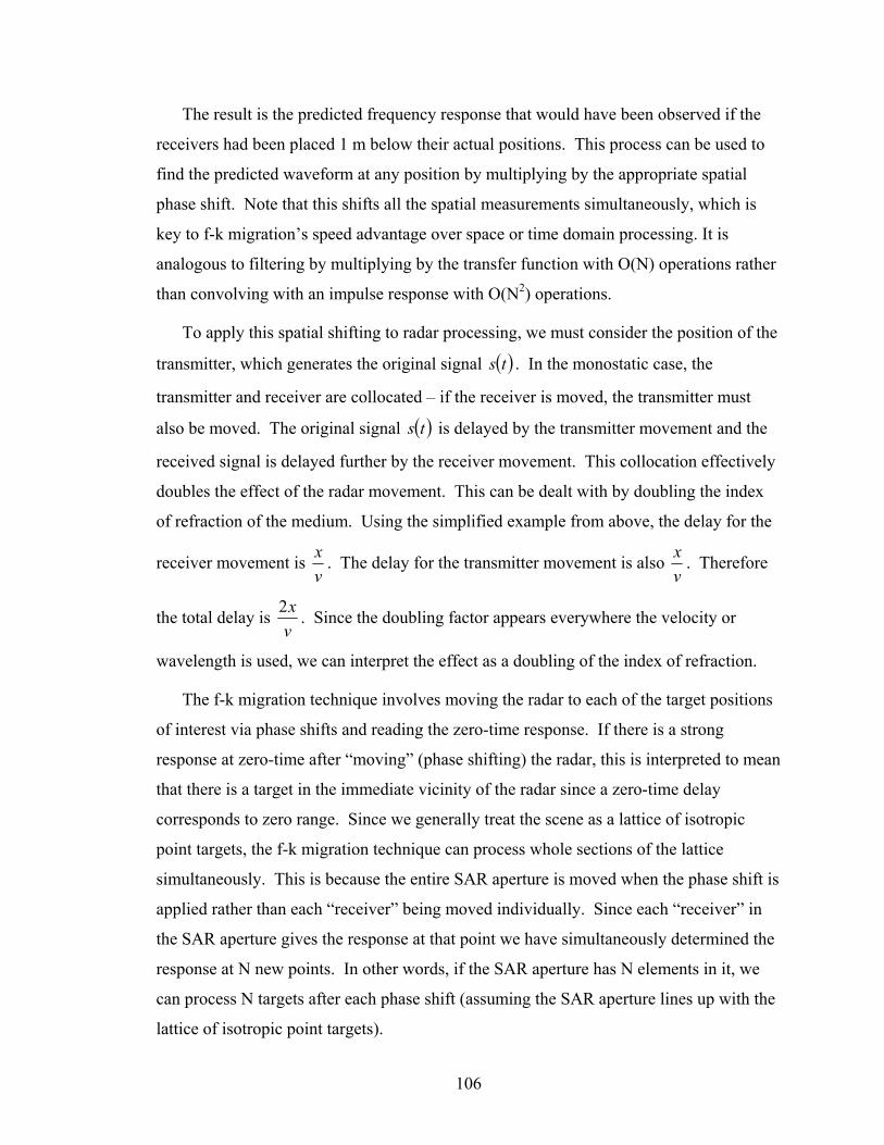
106

The result is the predicted frequency response that would have been observed if the

receivers had been placed 1 m below their actual positions. This process can be used to

find the predicted waveform at any position by multiplying by the appropriate spatial

phase shift. Note that this shifts all the spatial measurements simultaneously, which is

key to f-k migration’s speed advantage over space or time domain processing. It is

analogous to filtering by multiplying by the transfer function with O(N) operations rather

than convolving with an impulse response with O(N2) operations.

To apply this spatial shifting to radar processing, we must consider the position of the

transmitter, which generates the original signal ( )ts . In the monostatic case, the

transmitter and receiver are collocated – if the receiver is moved, the transmitter must

also be moved. The original signal ( )ts is delayed by the transmitter movement and the

received signal is delayed further by the receiver movement. This collocation effectively

doubles the effect of the radar movement. This can be dealt with by doubling the index

of refraction of the medium. Using the simplified example from above, the delay for the

receiver movement is vx . The delay for the transmitter movement is also

vx . Therefore

the total delay is vx2 . Since the doubling factor appears everywhere the velocity or

wavelength is used, we can interpret the effect as a doubling of the index of refraction.

The f-k migration technique involves moving the radar to each of the target positions

of interest via phase shifts and reading the zero-time response. If there is a strong

response at zero-time after “moving” (phase shifting) the radar, this is interpreted to mean

that there is a target in the immediate vicinity of the radar since a zero-time delay

corresponds to zero range. Since we generally treat the scene as a lattice of isotropic

point targets, the f-k migration technique can process whole sections of the lattice

simultaneously. This is because the entire SAR aperture is moved when the phase shift is

applied rather than each “receiver” being moved individually. Since each “receiver” in

the SAR aperture gives the response at that point we have simultaneously determined the

response at N new points. In other words, if the SAR aperture has N elements in it, we

can process N targets after each phase shift (assuming the SAR aperture lines up with the

lattice of isotropic point targets).

107

The final response needed by the processing is in the space-domain. As mentioned

above, the value at zero-time can be found by summing all of the frequency points. This

should be done before transforming from the wavenumber domain to the space domain

using the IFFT. By summing first, the number of IFFTs is reduced by a factor of 1−tN .

There are two caveats that need to be mentioned when using the f-k migration

algorithm. The first is that the process above assumes that the signal is band-limited in

space and time. If the signal were truly band-limited (infinite time signal) then there

would be no energy in parts of the data matrix that correspond to

λπ2

2222 =>++ kzyx kkk . However, there are portions of the frequency-wavenumber

data matrix that represent a combination of xk , yk , zk , and λ that require the wave to be

evanescent. In our case, the energy from the portions of the data matrix corresponding to

evanescent waves will be filtered out because wavenumber domain filtering is employed.

The second issue comes from the periodic nature of the discrete Fourier transform.

Because the signal is being represented discretely and circular convolution is being used

in the frequency domain, zero-padding may be necessary in some cases to remove

artifacts due to the non-linear nature of circular convolution (i.e. aliasing). This is

handled in the usual way by processing overlapping segments, truncating the segments so

that only the valid part is kept, and then concatenating these segments such that the

effective result is ordinary linear convolution.

The example above considered a mesh of space-time data. For this work, the data are

collected along a single line. Therefore only the time and x domain are sampled. To solve

for zk , yk is forced to be zero. While the restriction of data to a single line certainly

introduces errors, there are two reasons why this approach still produces a good quality

data product. The first is that the backscattering seen by the radar is primarily from the

negative z-direction suggesting that the yk component will be small. Secondly, the radar

employs cross-track (y-dimension) antenna arrays which narrow the beamwidth

significantly so that the yk domain is effectively low pass filtered. However, since we do

108

not fully sample the y-dimension there is still some ambiguity and this can be seen in the

migrated images shown in section 5.3.

Another technique we use is k-domain filtering and decimation. Filtering removes

noise energy (and evanescent wave energy as explained above) and decimation reduces

the number of operations performed by the migration routine. The procedure is identical

to the time/frequency-domain windowing and decimation described in section 4.3 – only

it is applied along the space/wavenumber-domain. The geometric interpretation of this

filter is worth describing since it provides a more intuitive understanding of the process.

The link between wavenumber and angle of arrival, θ , is illustrated in Fig. 5-3 and given

by

= −

2

1sink

xkθ .

k

kx

-kz

θ

θ

Spatial Samples

Wavefront

Fig. 5-3. Shows the relationship between the wavenumber and the angle of arrival.

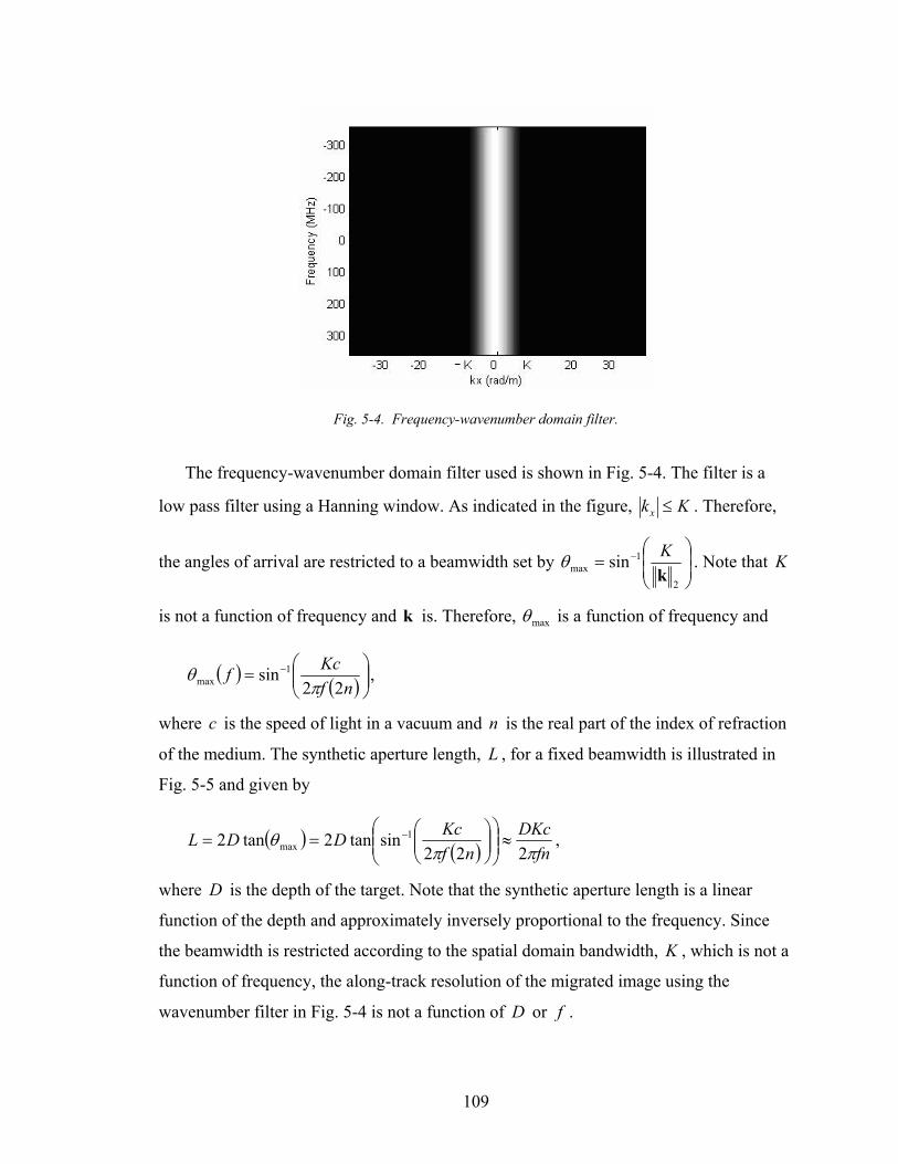
109

Fig. 5-4. Frequency-wavenumber domain filter.

The frequency-wavenumber domain filter used is shown in Fig. 5-4. The filter is a

low pass filter using a Hanning window. As indicated in the figure, Kkx ≤ . Therefore,

the angles of arrival are restricted to a beamwidth set by

= −

2

1max sin

kKθ . Note that K

is not a function of frequency and k is. Therefore, maxθ is a function of frequency and

( ) ( )

= −

nfKcf

22sin 1

max πθ ,

where c is the speed of light in a vacuum and n is the real part of the index of refraction

of the medium. The synthetic aperture length, L , for a fixed beamwidth is illustrated in

Fig. 5-5 and given by

( ) ( ) fnDKc

nfKcDDL

ππθ

222sintan2tan2 1

max ≈

== − ,

where D is the depth of the target. Note that the synthetic aperture length is a linear

function of the depth and approximately inversely proportional to the frequency. Since

the beamwidth is restricted according to the spatial domain bandwidth, K , which is not a

function of frequency, the along-track resolution of the migrated image using the

wavenumber filter in Fig. 5-4 is not a function of D or f .

110

θMax

Synthetic Aperture Length, L

D

Fig. 5-5. Shows the relationship between the synthetic aperture length, L , and the maximum angle of

arrival maxθ .

As mentioned in the introduction, f-k migration handles propagation in layered media

very naturally. We use the dielectric models developed in section 2.1 to generate an

approximated discrete depth-permittivity profile. Let nzzz ,2,1, ,,, ∆∆∆ K be a sequence

denoting the thickness of each layer and nnnn ,,, 21 K be the corresponding index of

refraction for each layer. Only the real part of the index of refraction is used so that the

migration algorithm corrects for phase only. The filter coefficients for the f-k migration

algorithm are then generated in an iterative manner by finding the transfer function

matrix for each layer and then multiplying these together. Using the development

described above to find the phase shift for each layer, we find the signal after the mth

layer to be

( ) ( ) ( )( )∏=

∆⋅−=m

ppzxpzxxm kfjkkfSkfS

1,,0 ,exp,, ,

where the solution for the z-component of the wavenumber, ( )xpz kfk ,, , is now a function

of the layer number.

The final adaptation to the algorithm was to incorporate the radar’s sample window

delay. Because of data rate limitations, the radar does not begin to record data at time

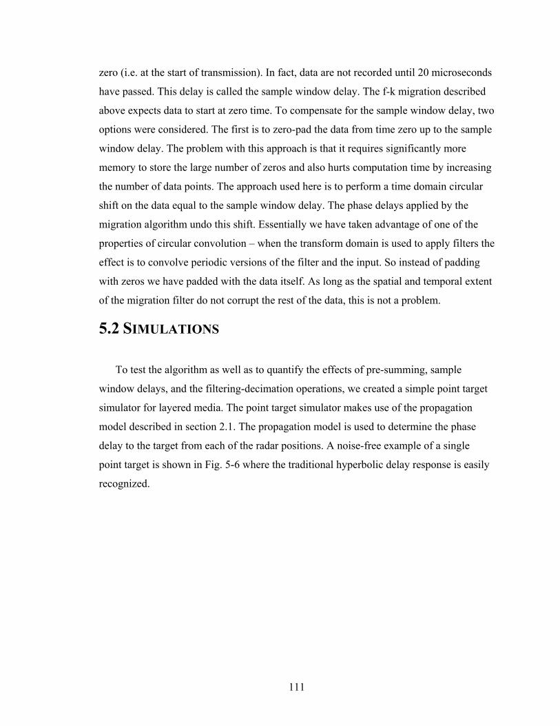
111

zero (i.e. at the start of transmission). In fact, data are not recorded until 20 microseconds

have passed. This delay is called the sample window delay. The f-k migration described

above expects data to start at zero time. To compensate for the sample window delay, two

options were considered. The first is to zero-pad the data from time zero up to the sample

window delay. The problem with this approach is that it requires significantly more

memory to store the large number of zeros and also hurts computation time by increasing

the number of data points. The approach used here is to perform a time domain circular

shift on the data equal to the sample window delay. The phase delays applied by the

migration algorithm undo this shift. Essentially we have taken advantage of one of the

properties of circular convolution – when the transform domain is used to apply filters the

effect is to convolve periodic versions of the filter and the input. So instead of padding

with zeros we have padded with the data itself. As long as the spatial and temporal extent

of the migration filter do not corrupt the rest of the data, this is not a problem.

5.2 SIMULATIONS

To test the algorithm as well as to quantify the effects of pre-summing, sample

window delays, and the filtering-decimation operations, we created a simple point target

simulator for layered media. The point target simulator makes use of the propagation

model described in section 2.1. The propagation model is used to determine the phase

delay to the target from each of the radar positions. A noise-free example of a single

point target is shown in Fig. 5-6 where the traditional hyperbolic delay response is easily

recognized.

112

Fig. 5-6. Example of a simulated point target with along-track hardware averages and pulse compression.

The target is located at a depth of 50 m and an along-track position of 0 m.

The migration algorithm applied without pre-summing, sample window delay, and

the filtering-decimation is shown in Fig. 5-7.

Fig. 5-7. Ideal migration with Hanning along-track windowing and boxcar time-domain windowing.

113

Pre-summing as explained in section 4.3 is effectively convolution in the spatial

domain with a boxcar window. This creates a sinc-squared radiation pattern in the along-

track dimension. Fig. 5-8 a) and b) show the transform domain before and after pre-

summing. The signal is bandpass between 120-300 MHz. The hour glass shape is because

of the evanescent waves (note that at DC there is no spatial bandwidth since DC waves

do not “travel”). If decimation is applied without proper space-domain filtering, the large

sidelobes will alias into the visual region and degrade the migrated image. Fig. 5-8 c)

shows the transform domain after low-pass filtering with a Hanning window. Decimation

can now be applied to the data.

Fig. 5-8. Example of pre-summing in the transform domain a) before pre-summing b) after pre-summing

and c) after spatial filtering.

The migrated image with pre-summing and spatial filtering is shown in Fig. 5-9.

Time-domain filtering and decimation has also been applied. Note that by lowering the

spatial bandwidth of the signal we have degraded the resolution since this shortens the

114

synthetic aperture length. Ordinarily this is not desirable unless signal characteristics or

processing requirements limit the aperture that can be used.

Fig. 5-9. Migration with pre-summing and spatial filtering.

As explained in the previous section, the sample window delay of the radar system is

greater than zero. The effect of a non-zero sample window delay corresponding to

approximately 30 m migrated with circular shifting is shown in Fig. 5-10. The migrated

image starts at a larger depth, but there is no effect on signal quality.

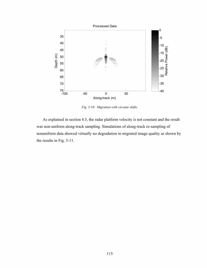
115

Along-track (m)

Dep

th (m

)

Processed Data

-100 -50 0 50

35

40

45

50

55

60

65

70

75

Rel

ativ

e P

ower

(dB

)

-40

-35

-30

-25

-20

-15

-10

-5

0

Fig. 5-10. Migration with circular shifts.

As explained in section 4.5, the radar platform velocity is not constant and the result

was non-uniform along-track sampling. Simulations of along-track re-sampling of

nonuniform data showed virtually no degradation in migrated image quality as shown by

the results in Fig. 5-11.

116

Fig. 5-11. Migration showing the effect of platform velocity variance for nonuniformly sampled data with

differing amounts of variance in the platform velocity. Note that there is no visual degradation in the

images.

Fig. 5-12. Velocity profile used to generate the above migrated image.

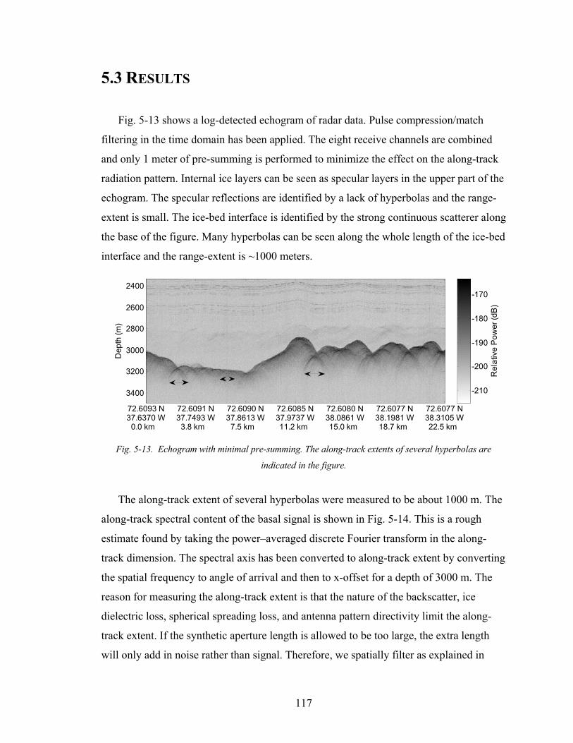
117

5.3 RESULTS

Fig. 5-13 shows a log-detected echogram of radar data. Pulse compression/match

filtering in the time domain has been applied. The eight receive channels are combined

and only 1 meter of pre-summing is performed to minimize the effect on the along-track

radiation pattern. Internal ice layers can be seen as specular layers in the upper part of the

echogram. The specular reflections are identified by a lack of hyperbolas and the range-

extent is small. The ice-bed interface is identified by the strong continuous scatterer along

the base of the figure. Many hyperbolas can be seen along the whole length of the ice-bed

interface and the range-extent is ~1000 meters.

72.6093 N37.6370 W

0.0 km

72.6091 N37.7493 W

3.8 km

72.6090 N37.8613 W

7.5 km

72.6085 N37.9737 W11.2 km

72.6080 N38.0861 W15.0 km

72.6077 N38.1981 W18.7 km

72.6077 N38.3105 W22.5 km

Dep

th (m

)

2400

2600

2800

3000

3200

3400

Rel

ativ

e P

ower

(dB

)

-210

-200

-190

-180

-170

Fig. 5-13. Echogram with minimal pre-summing. The along-track extents of several hyperbolas are

indicated in the figure.

The along-track extent of several hyperbolas were measured to be about 1000 m. The

along-track spectral content of the basal signal is shown in Fig. 5-14. This is a rough

estimate found by taking the power–averaged discrete Fourier transform in the along-

track dimension. The spectral axis has been converted to along-track extent by converting

the spatial frequency to angle of arrival and then to x-offset for a depth of 3000 m. The

reason for measuring the along-track extent is that the nature of the backscatter, ice

dielectric loss, spherical spreading loss, and antenna pattern directivity limit the along-

track extent. If the synthetic aperture length is allowed to be too large, the extra length

will only add in noise rather than signal. Therefore, we spatially filter as explained in

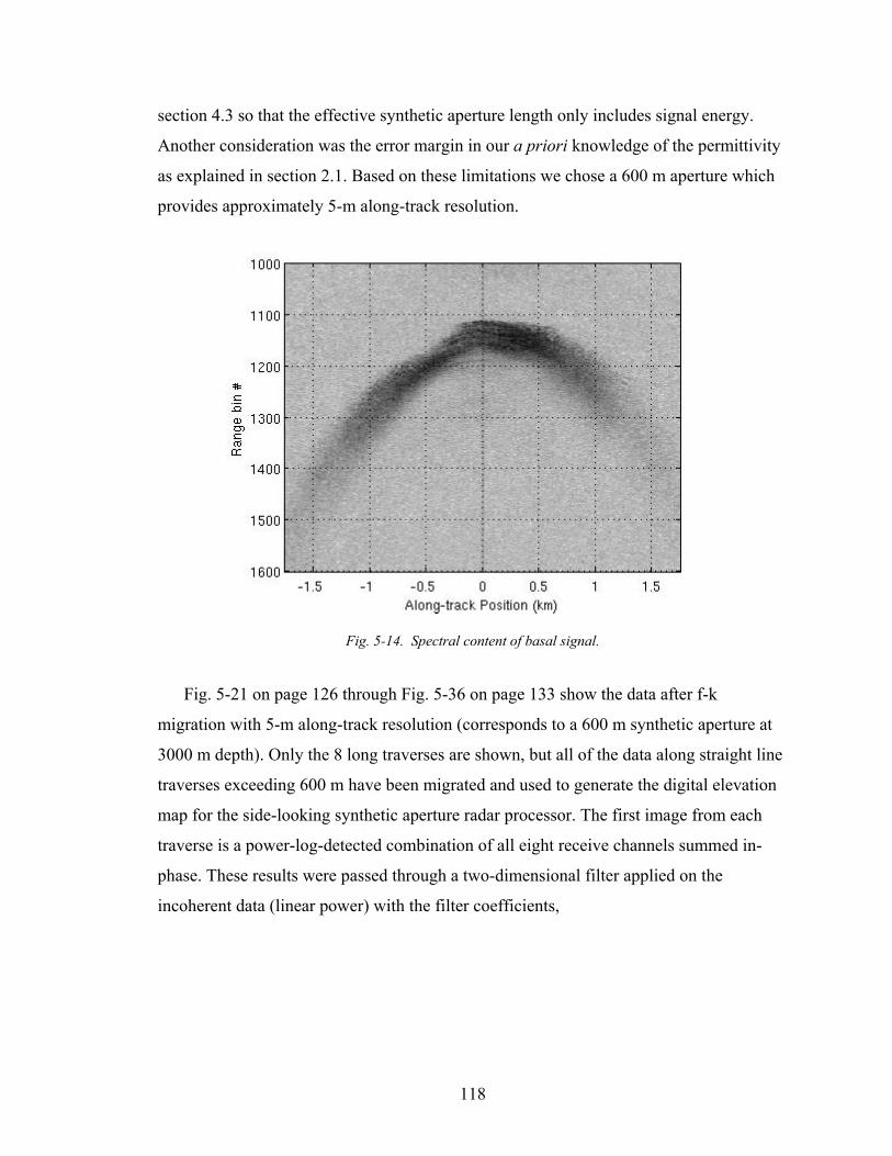
118

section 4.3 so that the effective synthetic aperture length only includes signal energy.

Another consideration was the error margin in our a priori knowledge of the permittivity

as explained in section 2.1. Based on these limitations we chose a 600 m aperture which

provides approximately 5-m along-track resolution.

Fig. 5-14. Spectral content of basal signal.

Fig. 5-21 on page 126 through Fig. 5-36 on page 133 show the data after f-k

migration with 5-m along-track resolution (corresponds to a 600 m synthetic aperture at

3000 m depth). Only the 8 long traverses are shown, but all of the data along straight line

traverses exceeding 600 m have been migrated and used to generate the digital elevation

map for the side-looking synthetic aperture radar processor. The first image from each

traverse is a power-log-detected combination of all eight receive channels summed in-

phase. These results were passed through a two-dimensional filter applied on the

incoherent data (linear power) with the filter coefficients,

119

111111111111111

151 ,

where the first dimension is along the depth axis and the second-dimension is parallel to

the along-track axis. The effective resolution after filtering is 5 m in depth and 15 m in

along-track. The second image from each traverse is an interferogram. The interferogram

is formed by 1) summing the migrated image from channels 1 and 2, 2) summing the

migrated images from channels 7 and 8, and 3) taking the component-wise conjugate

multiplication of the resultant sums:

*8channelreceive7channelreceive2channelreceive1channelreceive +⋅+ .

The effective baseline is small at 3.528 meters or 5.2528.3528.3==

cfnsnow

λ wavelengths,

which is why only four fringes are seen. The magnitude of the interferogram is processed

in the same way as the first image: filtering and power-log detection. The magnitude is an

indication of the coherence between the two summed images and provides an indication

of the interferometric quality of the phase information. The phase is magnitude detected

and then median filtered with an extent of five pixels in each dimension. The reason for

the magnitude detection is because there is left-right ambiguity in range. This means that

scattering from either side of the radar in the cross-track dimension arrive simultaneously

at the radar as shown in Fig. 5-15. Because of the simultaneous arrival of these two

signals that have equal and opposite phase, the resultant plot tends to look cluttered. By

taking the magnitude of the phase, the result tends to produce cleaner and more obvious

fringes at the expense of having complete left-right ambiguity. The value of the phase is

that it provides elevation angle information, albeit modulo 2π.

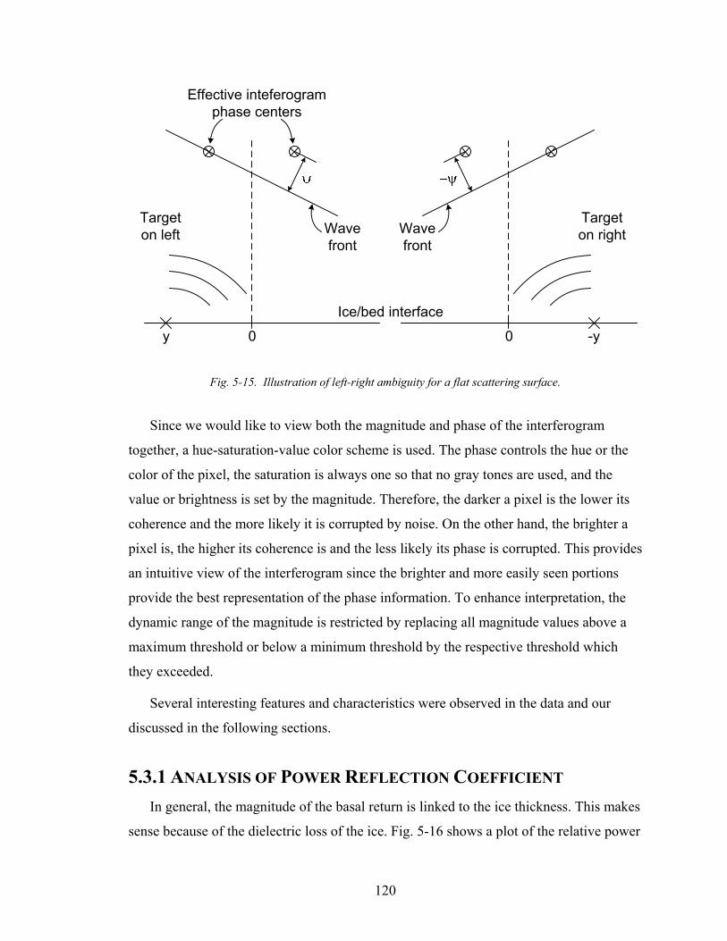
120

Target on right

Ice/bed interface

Target on left

Effective inteferogram phase centers

Wave front

Wave front

0y -y0

Fig. 5-15. Illustration of left-right ambiguity for a flat scattering surface.

Since we would like to view both the magnitude and phase of the interferogram

together, a hue-saturation-value color scheme is used. The phase controls the hue or the

color of the pixel, the saturation is always one so that no gray tones are used, and the

value or brightness is set by the magnitude. Therefore, the darker a pixel is the lower its

coherence and the more likely it is corrupted by noise. On the other hand, the brighter a

pixel is, the higher its coherence is and the less likely its phase is corrupted. This provides

an intuitive view of the interferogram since the brighter and more easily seen portions

provide the best representation of the phase information. To enhance interpretation, the

dynamic range of the magnitude is restricted by replacing all magnitude values above a

maximum threshold or below a minimum threshold by the respective threshold which

they exceeded.

Several interesting features and characteristics were observed in the data and our

discussed in the following sections.

5.3.1 ANALYSIS OF POWER REFLECTION COEFFICIENT In general, the magnitude of the basal return is linked to the ice thickness. This makes

sense because of the dielectric loss of the ice. Fig. 5-16 shows a plot of the relative power

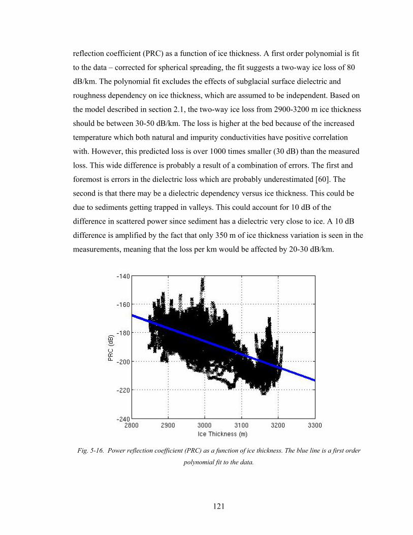
121

reflection coefficient (PRC) as a function of ice thickness. A first order polynomial is fit

to the data – corrected for spherical spreading, the fit suggests a two-way ice loss of 80

dB/km. The polynomial fit excludes the effects of subglacial surface dielectric and

roughness dependency on ice thickness, which are assumed to be independent. Based on

the model described in section 2.1, the two-way ice loss from 2900-3200 m ice thickness

should be between 30-50 dB/km. The loss is higher at the bed because of the increased

temperature which both natural and impurity conductivities have positive correlation

with. However, this predicted loss is over 1000 times smaller (30 dB) than the measured

loss. This wide difference is probably a result of a combination of errors. The first and

foremost is errors in the dielectric loss which are probably underestimated [60]. The

second is that there may be a dielectric dependency versus ice thickness. This could be

due to sediments getting trapped in valleys. This could account for 10 dB of the

difference in scattered power since sediment has a dielectric very close to ice. A 10 dB

difference is amplified by the fact that only 350 m of ice thickness variation is seen in the

measurements, meaning that the loss per km would be affected by 20-30 dB/km.

Fig. 5-16. Power reflection coefficient (PRC) as a function of ice thickness. The blue line is a first order

polynomial fit to the data.

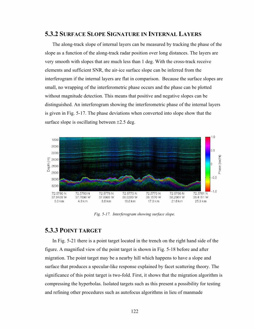
122

5.3.2 SURFACE SLOPE SIGNATURE IN INTERNAL LAYERS The along-track slope of internal layers can be measured by tracking the phase of the

slope as a function of the along-track radar position over long distances. The layers are

very smooth with slopes that are much less than 1 deg. With the cross-track receive

elements and sufficient SNR, the air-ice surface slope can be inferred from the

interferogram if the internal layers are flat in comparison. Because the surface slopes are

small, no wrapping of the interferometric phase occurs and the phase can be plotted

without magnitude detection. This means that positive and negative slopes can be

distinguished. An interferogram showing the interferometric phase of the internal layers

is given in Fig. 5-17. The phase deviations when converted into slope show that the

surface slope is oscillating between ±2.5 deg.

Fig. 5-17. Interferogram showing surface slope.

5.3.3 POINT TARGET In Fig. 5-21 there is a point target located in the trench on the right hand side of the

figure. A magnified view of the point target is shown in Fig. 5-18 before and after

migration. The point target may be a nearby hill which happens to have a slope and

surface that produces a specular-like response explained by facet scattering theory. The

significance of this point target is two-fold. First, it shows that the migration algorithm is

compressing the hyperbolas. Isolated targets such as this present a possibility for testing

and refining other procedures such as autofocus algorithms in lieu of manmade

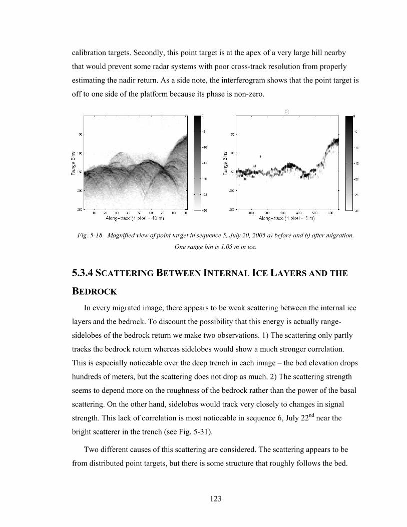
123

calibration targets. Secondly, this point target is at the apex of a very large hill nearby

that would prevent some radar systems with poor cross-track resolution from properly

estimating the nadir return. As a side note, the interferogram shows that the point target is

off to one side of the platform because its phase is non-zero.

Fig. 5-18. Magnified view of point target in sequence 5, July 20, 2005 a) before and b) after migration.

One range bin is 1.05 m in ice.

5.3.4 SCATTERING BETWEEN INTERNAL ICE LAYERS AND THE

BEDROCK In every migrated image, there appears to be weak scattering between the internal ice

layers and the bedrock. To discount the possibility that this energy is actually range-

sidelobes of the bedrock return we make two observations. 1) The scattering only partly

tracks the bedrock return whereas sidelobes would show a much stronger correlation.

This is especially noticeable over the deep trench in each image – the bed elevation drops

hundreds of meters, but the scattering does not drop as much. 2) The scattering strength

seems to depend more on the roughness of the bedrock rather than the power of the basal

scattering. On the other hand, sidelobes would track very closely to changes in signal

strength. This lack of correlation is most noticeable in sequence 6, July 22nd near the

bright scatterer in the trench (see Fig. 5-31).

Two different causes of this scattering are considered. The scattering appears to be

from distributed point targets, but there is some structure that roughly follows the bed.

124

Unlike the specular layers above the scattering which have angles of arrival concentrated

in the nadir direction, an interferogram formed using the first and last receive channels

shows a wide range of angles of arrival. If the scattering is due to layers, the layering has

been disrupted – most likely because of ice flow so close to the very rough bed. An

interesting note is the rather rapid change from specular layering to this diffuse scattering.

It is almost as if there is a sudden change in the flow regimes of the ice. The other

possibility for scattering is englacial debris, but this seems unlikely given that both the

GRIP and GISP2 cores contained very low concentrations of debris [53].

5.3.5 BRIGHT TARGET AT BOTTOM OF TRENCH A 250 m long bright target with a slope of 1-2 deg is located at the bottom of the

trench that runs aside the GRIP borehole. In the region surveyed, this target is located in

the narrowest portion of the trench as shown by the digital bed elevation map in Fig.

5-38. The relative signal strength is plotted in Fig. 5-19 after being passed through a 100

m moving average filter and is approximately 30 dB stronger than neighboring targets.

Based on the interferogram, the target is directly beneath the radar platform since the

phase is zero. The pre-migrated data show that the raw scattered energy is also

significantly higher. There are also hyperbolas present – suggesting that the surface may

not specular. Because the GRIP bore hole is only a few km from the target, we used the

bottom 50 m of the temperature profile from GRIP to extrapolate the temperature down

to the target depth of 3185 m as shown in Fig. 5-20. The estimated pressure melting

temperature is about -2.4 C [46]. If the linear approximation for temperature is correct,

the temperature at the base is -4 C or 1.6 C above the melting point. With radiometrically

calibrated basal scattering data, the absolute scattering strength could be inferred and

thereby an estimate of the dielectric of the basal material. Unfortunately, due to the large

error bars associated with the ice loss only a relative measure is possible.

125

Fig. 5-19. Shows signal strength of peak return as a function of along-track position. The brightness of the

target is about 30 dB stronger than neighboring targets after f-k migration.

Fig. 5-20. Temperature of basal ice extrapolated to 3400 m ice thickness from the last 50 m of the

temperature record at GRIP. The expected pressure melting temperature (approximated at -2.4 C is shown)

as is the target depth of 3185 m.

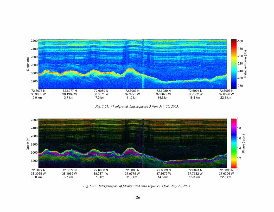
126

72.6077 N38.3065 W

0.0 km

72.6077 N38.1969 W

3.7 km

72.6080 N38.0871 W

7.3 km

72.6083 N37.9775 W11.0 km

72.6089 N37.8679 W14.6 km

72.6091 N37.7582 W18.3 km

72.6093 N37.6396 W22.3 km

Dep

th (m

)

2200

2400

2600

2800

3000

3200

Rel

ativ

e P

ower

(dB

)

-280

-260

-240

-220

-200

-180

-160

Fig. 5-21. f-k migrated data sequence 5 from July 20, 2005.

72.6077 N38.3065 W

0.0 km

72.6077 N38.1969 W

3.7 km

72.6080 N38.0871 W

7.3 km

72.6083 N37.9775 W11.0 km

72.6089 N37.8679 W14.6 km

72.6091 N37.7582 W18.3 km

72.6093 N37.6396 W22.3 km

Dep

th (m

)

2200

2400

2600

2800

3000

3200

Pha

se (r

ad/ π

)

0

0.2

0.4

0.6

0.8

1

Fig. 5-22. Interferogram of f-k migrated data sequence 5 from July 20, 2005.

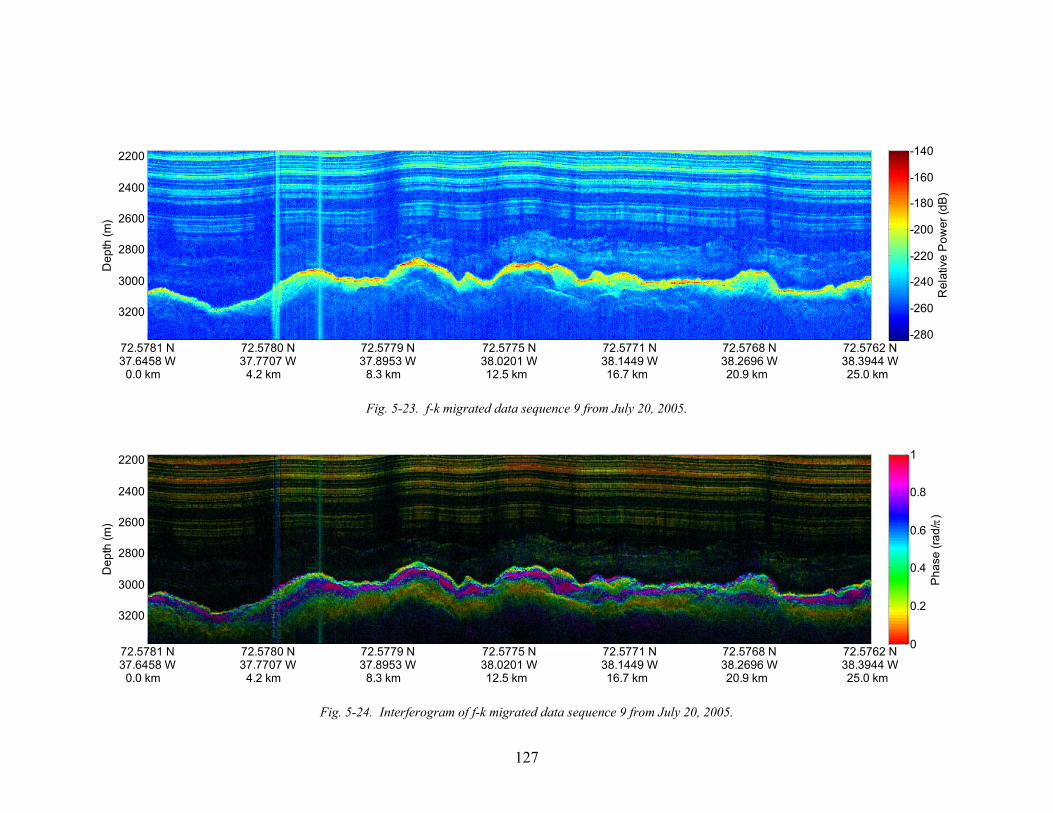
127

72.5781 N37.6458 W0.0 km

72.5780 N37.7707 W

4.2 km

72.5779 N37.8953 W

8.3 km

72.5775 N38.0201 W12.5 km

72.5771 N38.1449 W16.7 km

72.5768 N38.2696 W20.9 km

72.5762 N38.3944 W25.0 km

Dep

th (m

)

2200

2400

2600

2800

3000

3200

Rel

ativ

e P

ower

(dB

)

-280

-260

-240

-220

-200

-180

-160

-140


72.5781 N37.6458 W0.0 km

72.5780 N37.7707 W

4.2 km

72.5779 N37.8953 W

8.3 km

72.5775 N38.0201 W12.5 km

72.5771 N38.1449 W16.7 km

72.5768 N38.2696 W20.9 km

72.5762 N38.3944 W25.0 km

Dep

th (m

)

2200

2400

2600

2800

3000

3200

Pha

se (r

ad/ π

)

0

0.2

0.4

0.6

0.8

1


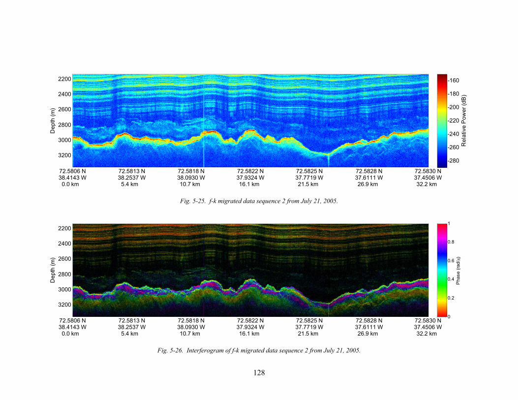
128

72.5806 N38.4143 W0.0 km

72.5813 N38.2537 W

5.4 km

72.5818 N38.0930 W10.7 km

72.5822 N37.9324 W16.1 km

72.5825 N37.7719 W21.5 km

72.5828 N37.6111 W26.9 km

72.5830 N37.4506 W32.2 km

Dep

th (m

)

2200

2400

2600

2800

3000

3200

Rel

ativ

e P

ower

(dB

)

-280

-260

-240

-220

-200

-180

-160


72.5806 N38.4143 W0.0 km

72.5813 N38.2537 W

5.4 km

72.5818 N38.0930 W10.7 km

72.5822 N37.9324 W16.1 km

72.5825 N37.7719 W21.5 km

72.5828 N37.6111 W26.9 km

72.5830 N37.4506 W32.2 km

Dep

th (m

)

2200

2400

2600

2800

3000

3200

Pha

se (r

ad/ π

)

0

0.2

0.4

0.6

0.8

1


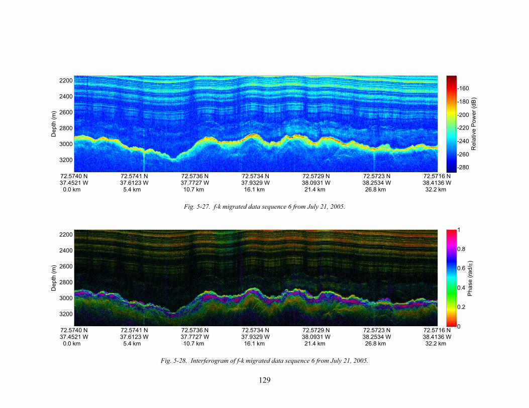
129

72.5740 N37.4521 W

0.0 km

72.5741 N37.6123 W

5.4 km

72.5736 N37.7727 W10.7 km

72.5734 N37.9329 W16.1 km

72.5729 N38.0931 W21.4 km

72.5723 N38.2534 W26.8 km

72.5716 N38.4136 W32.2 km

Dep

th (m

)

2200

2400

2600

2800

3000

3200

Rel

ativ

e P

ower

(dB

)

-280

-260

-240

-220

-200

-180

-160


72.5740 N37.4521 W

0.0 km

72.5741 N37.6123 W

5.4 km

72.5736 N37.7727 W10.7 km

72.5734 N37.9329 W16.1 km

72.5729 N38.0931 W21.4 km

72.5723 N38.2534 W26.8 km

72.5716 N38.4136 W32.2 km

Dep

th (m

)

2200

2400

2600

2800

3000

3200

Pha

se (r

ad/ π

)

0

0.2

0.4

0.6

0.8

1


130

72.5984 N38.3059 W

0.0 km

72.5993 N38.1659 W

4.7 km

72.5998 N38.0259 W

9.4 km

72.6003 N37.8859 W14.0 km

72.6005 N37.7458 W18.7 km

72.6007 N37.6058 W23.4 km

72.6009 N37.4657 W28.1 km

Dep

th (m

)

2200

2400

2600

2800

3000

3200

Rel

ativ

e P

ower

(dB

)

-280

-260

-240

-220

-200

-180

-160

-140


72.5984 N38.3059 W

0.0 km

72.5993 N38.1659 W

4.7 km

72.5998 N38.0259 W

9.4 km

72.6003 N37.8859 W14.0 km

72.6005 N37.7458 W18.7 km

72.6007 N37.6058 W23.4 km

72.6009 N37.4657 W28.1 km

Dep

th (m

)

2200

2400

2600

2800

3000

3200

Pha

se (r

ad/ π

)

0

0.2

0.4

0.6

0.8

1


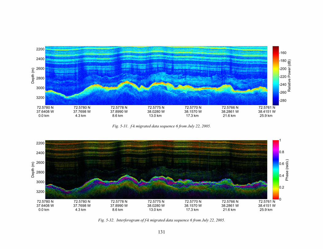
131

72.5780 N37.6408 W

0.0 km

72.5780 N37.7698 W

4.3 km

72.5778 N37.8990 W

8.6 km

72.5775 N38.0280 W13.0 km

72.5770 N38.1570 W17.3 km

72.5766 N38.2861 W21.6 km

72.5761 N38.4151 W25.9 km

Dep

th (m

)

2200

2400

2600

2800

3000

3200

Rel

ativ

e P

ower

(dB

)

-280

-260

-240

-220

-200

-180

-160


72.5780 N37.6408 W

0.0 km

72.5780 N37.7698 W

4.3 km

72.5778 N37.8990 W

8.6 km

72.5775 N38.0280 W13.0 km

72.5770 N38.1570 W17.3 km

72.5766 N38.2861 W21.6 km

72.5761 N38.4151 W25.9 km

Dep

th (m

)

2200

2400

2600

2800

3000

3200

Pha

se (r

ad/ π

)

0

0.2

0.4

0.6

0.8

1


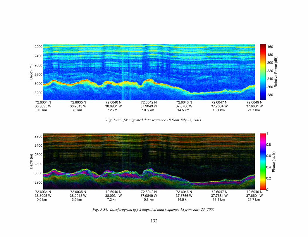
132

72.6034 N38.3095 W

0.0 km

72.6035 N38.2013 W

3.6 km

72.6040 N38.0931 W

7.2 km

72.6042 N37.9849 W10.8 km

72.6046 N37.8766 W14.5 km

72.6047 N37.7684 W18.1 km

72.6049 N37.6601 W21.7 km

Dep

th (m

)

2200

2400

2600

2800

3000

3200

Rel

ativ

e P

ower

(dB

)

-280

-260

-240

-220

-200

-180

-160


72.6034 N38.3095 W

0.0 km

72.6035 N38.2013 W

3.6 km

72.6040 N38.0931 W

7.2 km

72.6042 N37.9849 W10.8 km

72.6046 N37.8766 W14.5 km

72.6047 N37.7684 W18.1 km

72.6049 N37.6601 W21.7 km

Dep

th (m

)

2200

2400

2600

2800

3000

3200

Pha

se (r

ad/ π

)

0

0.2

0.4

0.6

0.8

1


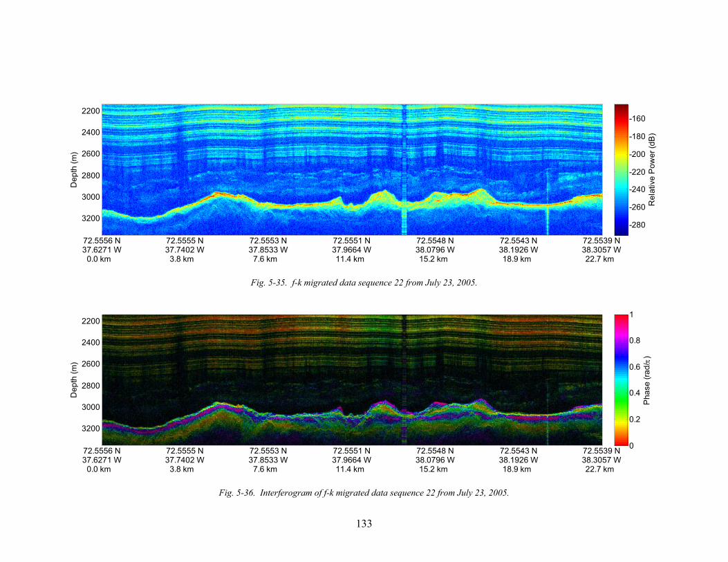
133

72.5556 N37.6271 W

0.0 km

72.5555 N37.7402 W

3.8 km

72.5553 N37.8533 W

7.6 km

72.5551 N37.9664 W11.4 km

72.5548 N38.0796 W15.2 km

72.5543 N38.1926 W18.9 km

72.5539 N38.3057 W22.7 km

Dep

th (m

)

2200

2400

2600

2800

3000

3200

Rel

ativ

e P

ower

(dB

)

-280

-260

-240

-220

-200

-180

-160


72.5556 N37.6271 W

0.0 km

72.5555 N37.7402 W

3.8 km

72.5553 N37.8533 W

7.6 km

72.5551 N37.9664 W11.4 km

72.5548 N38.0796 W15.2 km

72.5543 N38.1926 W18.9 km

72.5539 N38.3057 W22.7 km

Dep

th (m

)

2200

2400

2600

2800

3000

3200

Pha

se (r

ad/ π

)

0

0.2

0.4

0.6

0.8

1


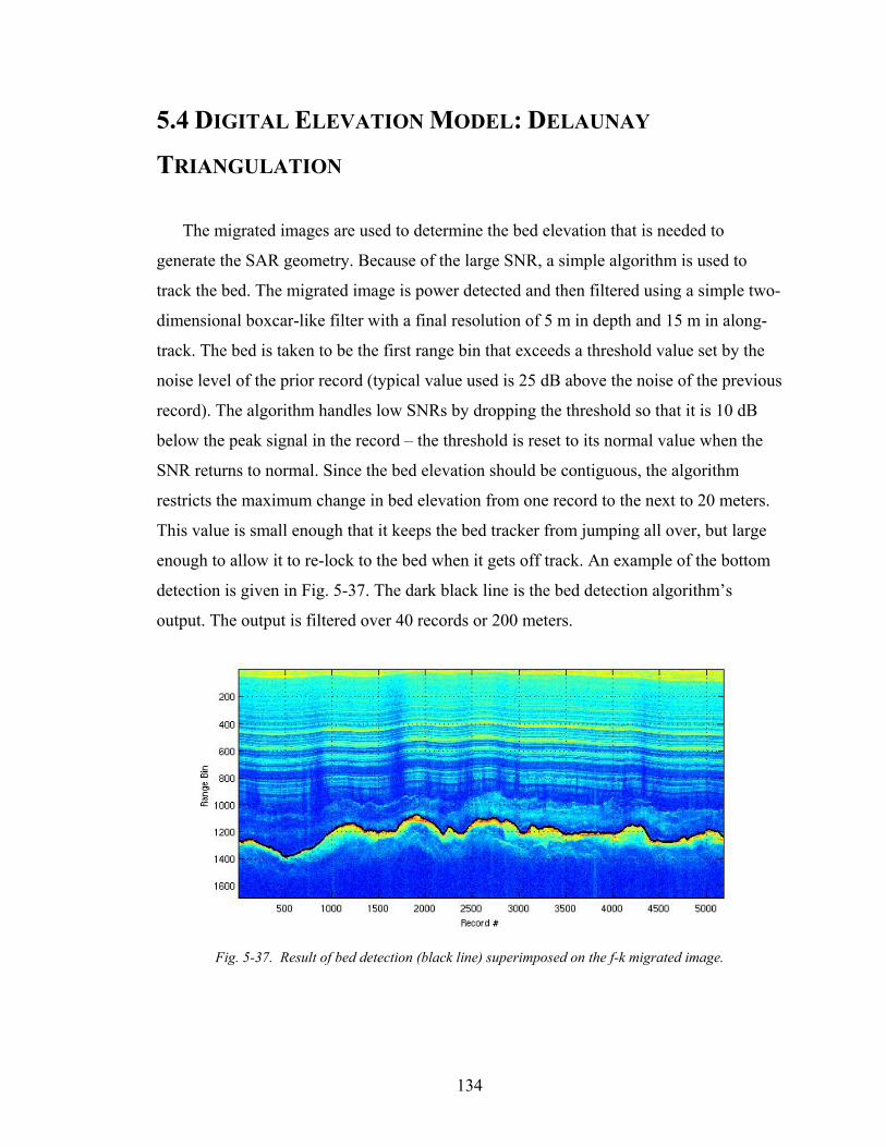
134

5.4 DIGITAL ELEVATION MODEL: DELAUNAY

TRIANGULATION

The migrated images are used to determine the bed elevation that is needed to

generate the SAR geometry. Because of the large SNR, a simple algorithm is used to

track the bed. The migrated image is power detected and then filtered using a simple two-

dimensional boxcar-like filter with a final resolution of 5 m in depth and 15 m in along-

track. The bed is taken to be the first range bin that exceeds a threshold value set by the

noise level of the prior record (typical value used is 25 dB above the noise of the previous

record). The algorithm handles low SNRs by dropping the threshold so that it is 10 dB

below the peak signal in the record – the threshold is reset to its normal value when the

SNR returns to normal. Since the bed elevation should be contiguous, the algorithm

restricts the maximum change in bed elevation from one record to the next to 20 meters.

This value is small enough that it keeps the bed tracker from jumping all over, but large

enough to allow it to re-lock to the bed when it gets off track. An example of the bottom

detection is given in Fig. 5-37. The dark black line is the bed detection algorithm’s

output. The output is filtered over 40 records or 200 meters.

Fig. 5-37. Result of bed detection (black line) superimposed on the f-k migrated image.

135

Once all the migrated images are run through the bed tracking algorithm a digital

elevation map is generated from the traverse lines using the linear Delaunay triangulation

algorithm. The results are shown in Fig. 5-38. The traverse lines are in black and

represent the locations of the data points. The areas in between are interpolated. Since

ground truth data exist for the ice thickness at GISP2 and GRIP, a comparison with the

ice thickness used to generate the DEM is given in Table 5-1. There appears to be a bias

of about -15 meters in the ice thickness estimate. If the error is caused by a velocity error

in ice, a permittivity change of -0.03 would be needed to correct it. The difference may

be attributable to three other sources of error. The first is that the data are low-pass

filtered after bed tracking. The second is that a nearby hill would mask the actual bed

location. Finally, the bed estimate may be biased because the tracker chooses the first

range bin that exceeds a threshold set relative to the noise floor – if the signal is very

strong this may actually be a sidelobe of the actual bed reflection.

Fig. 5-38. Digital elevation map of subglacial bed generated from migrated images. GISP2 is marked by a

magenta circle and GRIP is marked by a red circle.

Table 5-1: Comparison of DEM with GRIP and GISP2 ground truth data. Borehole Ground Truth DEM Error

GRIP 3027.6 m 3015.3 m -12.3 m

GISP2 3047.9 m 3029.9 m -18.0 m

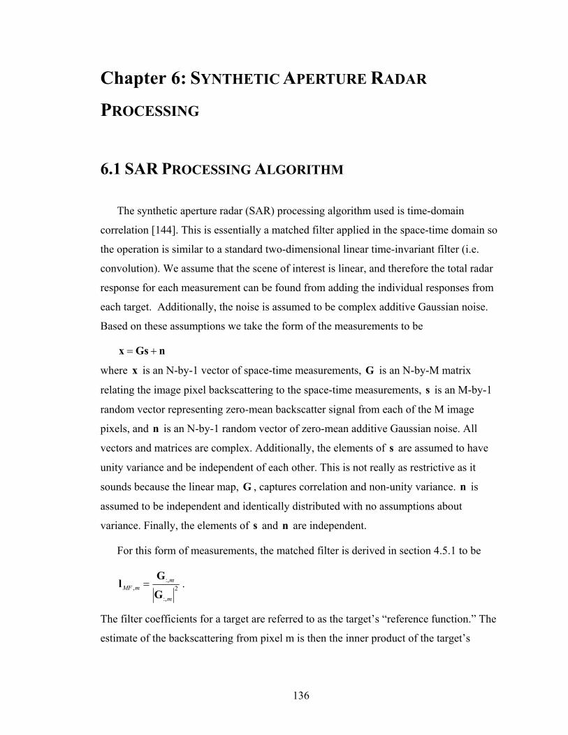
136

Chapter 6: SYNTHETIC APERTURE RADAR

PROCESSING

6.1 SAR PROCESSING ALGORITHM

The synthetic aperture radar (SAR) processing algorithm used is time-domain

correlation [144]. This is essentially a matched filter applied in the space-time domain so

the operation is similar to a standard two-dimensional linear time-invariant filter (i.e.

convolution). We assume that the scene of interest is linear, and therefore the total radar

response for each measurement can be found from adding the individual responses from

each target. Additionally, the noise is assumed to be complex additive Gaussian noise.

Based on these assumptions we take the form of the measurements to be

nGsx +=

where x is an N-by-1 vector of space-time measurements, G is an N-by-M matrix

relating the image pixel backscattering to the space-time measurements, s is an M-by-1

random vector representing zero-mean backscatter signal from each of the M image

pixels, and n is an N-by-1 random vector of zero-mean additive Gaussian noise. All

vectors and matrices are complex. Additionally, the elements of s are assumed to have

unity variance and be independent of each other. This is not really as restrictive as it

sounds because the linear map, G , captures correlation and non-unity variance. n is

assumed to be independent and identically distributed with no assumptions about

variance. Finally, the elements of s and n are independent.

For this form of measurements, the matched filter is derived in section 4.5.1 to be

2:,

:,,

m

mmMF

G

Gl = .

The filter coefficients for a target are referred to as the target’s “reference function.” The

estimate of the backscattering from pixel m is then the inner product of the target’s

137

reference function and the measurements: xlHmMFms ,ˆ = . This result is the same as the

traditional matched filter in that the filter coefficients are the conjugate of the expectation

of the SNR. The only difference is that a generic linear map is used to associate the

measurements with the image pixels. The linear map is determined using the radar

equation described in section 0. The targets in the SAR processor are approximated by a

set of isotropic point scatterers with frequency-independent complex weights. Therefore,

the scattering term in the radar equation, 0σA , is represented as a single isotropic point

scatterer.

Note that the radar equation only gives the magnitude response. To determine the

phase response of the system, propagation delays and equipment phase information must

be known. The propagation delay is found from refraction, path length and changes in

velocity. The equipment phase delay is determined from the measured S21 parameters of

the transmitter and receiver responses. To determine the path lengths requires knowledge

of how the ray was refracted along its traverse. This is dealt with using the ice sheet

model described in section 2.1.

The reason for operating in the space-time domain is to avoid traditional motion

compensation techniques that are required to uniformly fit the data to a straight line

trajectory in order to use Fourier techniques. In the case of nadir sounding, cross-track

motion produces virtually no effect on the imaging algorithm. On the other hand, cross-

track motion has a large effect on side-looking imaging algorithms. Because the ice sheet

is barren of visually identifiable objects that can be used to track off while driving, the

radar trajectory in this work has significant cross-track movement21. By processing in

space-time, G can easily account for these variations.

To keep the processing tractable in terms of computational complexity, several

techniques were used. The first is that the data are pulse compressed before SAR

processing to reduce the time-extent of a target’s scattered energy. Ideally, every

measurement is placed inside the measurement vector x . However, only a few samples

as determined by G actually contain significant energy from the target. This means that

21 A handheld GPS was used and provided heading information, but the resolution was coarse.

138

the size of x and G can be much smaller during the solution for a particular target. In

the algorithm used for this work, only eleven time samples – five on each side of the

main lobe – are used. This allows the magnitude and phase information of the main lobe

and the first few side lobes to be included.

The second simplification was to use along-track low-pass filtering followed by

down-sampling to reduce the number of spatial measurements included in x and G .

Decimation is limited by two factors:

1) The along-track filtering process removes the high spatial-frequency energy on the

edges of the hyperbola and thereby limits the maximum SAR aperture length.

2) The uniform re-sampling of the data required by the Fourier transform to apply

standard filtering techniques does not account for cross-track movement.

The two limitations interact with one another and both enforce requirements that need

to be satisfied. Limitation 1) is a standard trade-off that must be made in any SAR

application and is sometimes referred to as pre-summing (although we apply a true

spatial filter for reasons explained in section 5.2). The second limitation is dependent on

the accuracy of the platform heading. Since the averaging lengths to be considered are

less than 10 meters and given the limited mobility of the platform, the cross-track

movement is linear during averages. In other words, the vehicle does not change

directions fast enough to allow for significant oscillations in cross-track movement

during a single averaging interval. The filter before decimation then becomes not only a

low-pass filter in the along-track domain, but a low-pass filter in the cross-track domain.

Essentially, a rotation of the filter in the spatial domain corresponds to a rotation in the

wavenumber domain. For side-looking operation this can have serious implications

because we are interested in keeping the cross-track beamwidth wide enough to always

“see” the whole scene for the entire SAR aperture length. This is illustrated in Fig. 6-1. If

the heading was always zero, the filter width could be set exactly equal to the SAR

aperture length. However, for a non-zero heading the filter width must be enlarged so that

even after rotation the entire scene (hashed area) is still in the filter.

For over 99% of the measurements, the platform heading error from a straight line

trajectory is less than 10 deg. The swath width stretches to 1000 m on each side of the

139

platform. Therefore the effective SAR aperture length considered in limitation 1) must be

extended by ( ) m350deg10tan10002 =⋅ to allow for the non-zero headings.

Swath Width

Filter Width (Non-zero Heading)

Filter Width

SAR Aperture Length

Platform trajectory

x

y

z

Fig. 6-1. Relationship between SAR aperture length and filter width for a non-zero heading.

The SAR aperture length was restricted to 300 m (resulting in 10 m image resolution)

to keep the computational complexity at a manageable level. To increase it to 600 m

would result in a four times increase in the computation time. Based on the current

computation time of 560 hours for a 300 m aperture, the dataset would take more than

2000 hours to process. The primary purpose of this work is to show the feasibility and

value of side-looking SAR to subglacial beds, which the shorter aperture length does

effectively.

140

6.2 SIMULATIONS

As with the f-k migration routine, a target simulator is used to test the algorithm as

well as to fine-tune choices in window size, pre-summing, etc. A simulation of a single

point target is shown in Fig. 6-2 and the SAR processed result is shown in Fig. 6-3.

Several points came out of these simulations and these are listed here:

1. As noted above, pulse compression was applied before the data were sent to the

SAR processor. The time-domain windowing, Hanning, is also applied during the pulse

compression. No additional time-domain windowing is needed during the SAR

processing. The windowing could be applied in the SAR processor, but would be

degraded by the truncated time-domain correlation of only 11 time samples. A small

degradation in the cross-track/time-domain side lobe levels is seen when windowing is

performed in the SAR processor.

2. A Hanning window is used for spatial filtering during the pre-sum process – the

reasoning and purpose are the same as for f-k migration that are described in section 5.2.

As explained above, because of the non-zero heading, the spatial filter’s beamwidth used

for the SAR processor is wider. The filter used is twice as wide as what would have been

needed if we could have assumed zero-heading. Because the filter is twice as wide (600

m along-track versus 300 m along-track), the along-track decimation rate is also halved.

The end result being that the SAR processor is fed twice as many spatial samples,

because they are more finely spaced. The finer spacing, although doubling the processing

time, also reduced along-track sidelobes. This is because of the improved control of the

reference function over the synthetic aperture that finer sampling affords.

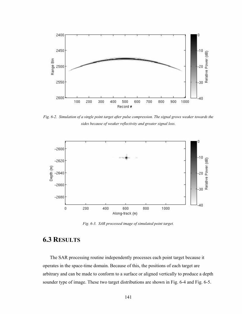
141

Fig. 6-2. Simulation of a single point target after pulse compression. The signal grows weaker towards the

sides because of weaker reflectivity and greater signal loss.

Fig. 6-3. SAR processed image of simulated point target.

6.3 RESULTS

The SAR processing routine independently processes each point target because it

operates in the space-time domain. Because of this, the positions of each target are

arbitrary and can be made to conform to a surface or aligned vertically to produce a depth

sounder type of image. These two target distributions are shown in Fig. 6-4 and Fig. 6-5.

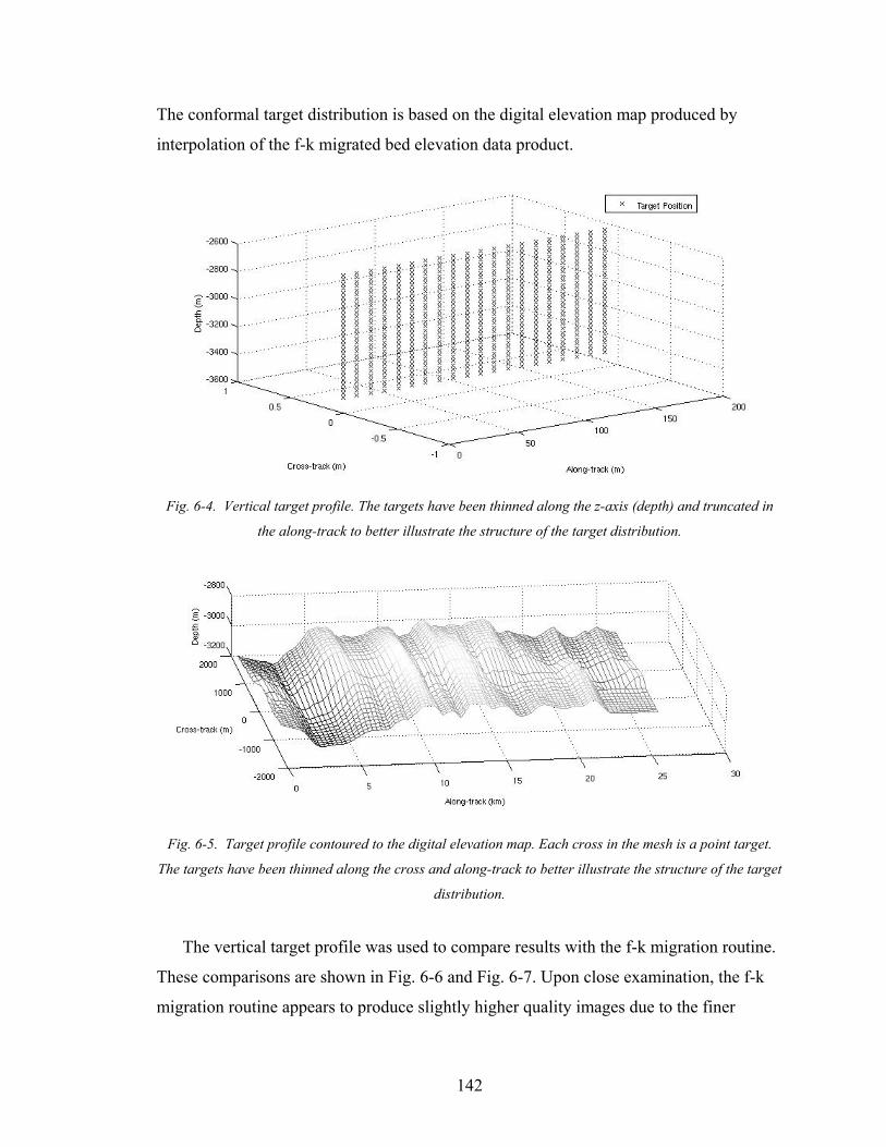
142

The conformal target distribution is based on the digital elevation map produced by

interpolation of the f-k migrated bed elevation data product.

Fig. 6-4. Vertical target profile. The targets have been thinned along the z-axis (depth) and truncated in

the along-track to better illustrate the structure of the target distribution.

Fig. 6-5. Target profile contoured to the digital elevation map. Each cross in the mesh is a point target.

The targets have been thinned along the cross and along-track to better illustrate the structure of the target

distribution.

The vertical target profile was used to compare results with the f-k migration routine.

These comparisons are shown in Fig. 6-6 and Fig. 6-7. Upon close examination, the f-k

migration routine appears to produce slightly higher quality images due to the finer

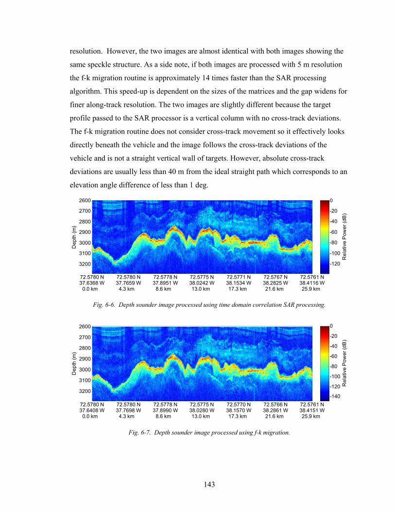
143

resolution. However, the two images are almost identical with both images showing the

same speckle structure. As a side note, if both images are processed with 5 m resolution

the f-k migration routine is approximately 14 times faster than the SAR processing

algorithm. This speed-up is dependent on the sizes of the matrices and the gap widens for

finer along-track resolution. The two images are slightly different because the target

profile passed to the SAR processor is a vertical column with no cross-track deviations.

The f-k migration routine does not consider cross-track movement so it effectively looks

directly beneath the vehicle and the image follows the cross-track deviations of the

vehicle and is not a straight vertical wall of targets. However, absolute cross-track

deviations are usually less than 40 m from the ideal straight path which corresponds to an

elevation angle difference of less than 1 deg.

72.5780 N37.6368 W

0.0 km

72.5780 N37.7659 W

4.3 km

72.5778 N37.8951 W

8.6 km

72.5775 N38.0242 W13.0 km

72.5771 N38.1534 W17.3 km

72.5767 N38.2825 W21.6 km

72.5761 N38.4116 W25.9 km

Dep

th (m

)

2600

2700

2800

2900

3000

3100

3200

Rel

ativ

e P

ower

(dB

)

-120

-100

-80

-60

-40

-20

0

Fig. 6-6. Depth sounder image processed using time domain correlation SAR processing.

72.5780 N37.6408 W

0.0 km

72.5780 N37.7698 W

4.3 km

72.5778 N37.8990 W

8.6 km

72.5775 N38.0280 W13.0 km

72.5770 N38.1570 W17.3 km

72.5766 N38.2861 W21.6 km

72.5761 N38.4151 W25.9 km

Dep

th (m

)

2600

2700

2800

2900

3000

3100

3200

Rel

ativ

e P

ower

(dB

)

-140

-120

-100

-80

-60

-40

-20

0

Fig. 6-7. Depth sounder image processed using f-k migration.

144

The conformal target distribution is used for creating the images of the subglacial

bed. The along-track positions are spaced by 10 m, which is the along-track resolution for

a 300 m aperture and 3000 m range. The cross-track positions are spaced so that the

distance between two targets projected onto a flat surface is equal to the range resolution

of the radar. Since there is substantial bed relief coupled with steep elevation angles (10

to 20 degrees incidence angle) a simple flat earth model could not be used. An example

of the geometric error induced by using a flat earth approximation is shown in Fig. 6-8.

For this simple example, a height error of errz causes a cross-track position error of

θtanerr

errzy = ,

where θ is the incidence angle. Since the incidence angle is related to the target’s

position relative to the radar by

∆∆

= −

zy1tanθ where y∆ and z∆ are the relative offsets

in each dimension, we have ∞→erry as 0→∆y . That is, targets close to nadir will have

the largest cross-track position errors. In the opposite extreme, for grazing angles

∞→∆y , then 2πθ → and 0→erry . Height errors at grazing angles do not create cross-

track position errors. Since we are operating with steep elevation angles, the cross-track

position errors will be large.

Fig. 6-8. Illustration of geometric errors induced by height errors in the scene.

Two common problems in SAR images are shadowing and layover and both are

related to the surface slope, σ , and the incidence angle, θ . Examples of both are shown

in Fig. 6-9. Shadowing occurs when the surface slope does not have line of sight with the

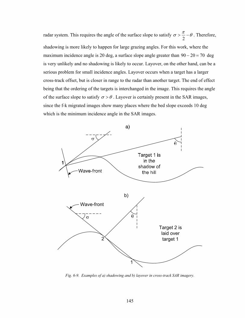
145

radar system. This requires the angle of the surface slope to satisfy θπσ −>2

. Therefore,

shadowing is more likely to happen for large grazing angles. For this work, where the

maximum incidence angle is 20 deg, a surface slope angle greater than 702090 =− deg

is very unlikely and no shadowing is likely to occur. Layover, on the other hand, can be a

serious problem for small incidence angles. Layover occurs when a target has a larger

cross-track offset, but is closer in range to the radar than another target. The end of effect

being that the ordering of the targets is interchanged in the image. This requires the angle

of the surface slope to satisfy θσ > . Layover is certainly present in the SAR images,

since the f-k migrated images show many places where the bed slope exceeds 10 deg

which is the minimum incidence angle in the SAR images.

2

1

Target 2 is laid over target 1

Wave-front

b)

Fig. 6-9. Examples of a) shadowing and b) layover in cross-track SAR imagery.

146

The SAR imagery presented in Fig. 6-13 on page 151 through Fig. 6-28 on page 158

is processed with the conformally mapped target distribution. Occasionally the actual bed

topography deviates far enough from the digital elevation map that the algorithm was

focusing to points within the ice rather than on the ice/bed interface. These errors are

identified by the dark blue patches on the side of the swath closest to the radar or 0 m

cross-track. An example of a surface profile that could lead to this is shown in Fig. 6-10.

The dark blue patches are caused by the SAR algorithm attempting to focus to points so

far above the actual bed that the range shells contain no bed scatterers. These height

errors are really a special case of layover where the swath targets are laid over the nadir

target. Therefore, a target at cross-track position y∆ which has a height error

θtanyzerr ∆> will not see any scatterers. Put another way, the average slope between the

target and nadir exceeds the incidence angle. As can be seen in the SAR results there are

a number of locations which are corrupted by this error.

147

Interpolated DEMActual

Surface

Bottom Estimates

Range shells which determined bottom estimates

Cross-track separation

between grid lines

a)

Fig. 6-10. Example of bed topography that could lead to severe DEM errors. The thickness estimate and

interpolated surface from three depth sounding passes are shown in a) and the effect on the SAR processor

is shown in b).

To illustrate a potential solution to this problem, a swath of SAR data are shown in

Fig. 6-11 beside an interferogram from f-k migration. The interferogram is from the

migrated data that was used to generate the digital elevation map the SAR image used at

500-m cross-track. Note how the patches of errors in the SAR line up with the largest

non-zero surface phases in the interferograms. The dark magenta color riding on the top

of the surface implies that the first echo in range is not from nadir, but from one side or

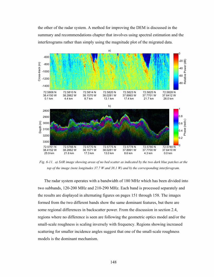
148

the other of the radar system. A method for improving the DEM is discussed in the

summary and recommendations chapter that involves using spectral estimation and the

interferograms rather than simply using the magnitude plot of the migrated data.

72.5806 N38.4150 W

0.1 km

72.5810 N38.2862 W

4.4 km

72.5814 N38.1570 W

8.7 km

72.5820 N38.0281 W13.1 km

72.5823 N37.8993 W17.4 km

72.5825 N37.7701 W21.7 km

72.5828 N37.6412 W26.0 km

Cro

ss-tr

ack

(m)

a)

-1400

-1200

-1000

-800

-600

Rel

ativ

e P

ower

(dB

)

-80

-60

-40

-20

0

72.5761 N38.4152 W25.9 km

72.5766 N38.2862 W21.6 km

72.5770 N38.1571 W17.3 km

72.5775 N38.0281 W13.0 km

72.5778 N37.8991 W

8.6 km

72.5780 N37.7700 W

4.3 km

72.5780 N37.6410 W

0.0 km

Dep

th (m

)

b)

2800

2900

3000

3100

3200

3300

Pha

se (r

ad/ π

)

0

0.2

0.4

0.6

0.8

1

Fig. 6-11. a) SAR image showing areas of no bed scatter as indicated by the two dark blue patches at the

top of the image (note longitudes 37.7 W and 38.1 W) and b) the corresponding interferogram.

The radar system operates with a bandwidth of 180 MHz which has been divided into

two subbands, 120-200 MHz and 210-290 MHz. Each band is processed separately and

the results are displayed in alternating figures on pages 151 through 158. The images

formed from the two different bands show the same dominant features, but there are

some regional differences in backscatter power. From the discussion in section 2.4,

regions where no difference is seen are following the geometric optics model and/or the

small-scale roughness is scaling inversely with frequency. Regions showing increased

scattering for smaller incidence angles suggest that one of the small-scale roughness

models is the dominant mechanism.

149

To reduce the effects of fading, 15 looks are taken. To do this, the data are passed

through a two-dimensional boxcar filter with 5 cross-track looks and 3 along-track looks.

The raw imaging resolution is 2-6 m in the cross-track by 10 m in the along-track. The

variation in the cross-track resolution is because of the relationship between the slant

range resolution, which is constant at 1 m and directly related to the inverse of the

bandwidth, and the ground range resolution, which is related to the slant range resolution

divided by the sine of the incidence angle. After filtering, the resolution is 10-30 m in the

cross-track by 30 m in the along-track.

For visualization the SAR images are normalized so that the mean power for each

cross-track position is made equal. The normalization function for each band is shown in

Fig. 6-12. The SAR processing algorithm actually focuses a continuous swath from -1500

to +1500, but due to left-right ambiguity issues the valid region excludes the center of the

swath from -500 to +500 m. The normalization function is the mean of the power for

each cross-track cell across all SAR images. As expected the signal power is strongest at

nadir or for small incidence angles and is weaker for greater incidence angles. There is a

slight left-right asymmetry which is probably due to the asymmetry in the feed structure

of the TEM horn antennas which are fed from the right-hand side (towards negative

cross-track position). The dip at nadir is due to height errors that place the nadir point

target above the surface. The SNR is fairly low beyond 1000 m from the center of the

swath as expected. The mosaic presented in section 6.4 uses the left and right portions of

the swath that are 500 m to 1000 m from the center.

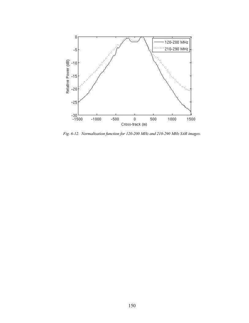
150

Fig. 6-12. Normalization function for 120-200 MHz and 210-290 MHz SAR images.

151

72.6077 N38.3105 W

0.0 km

72.6077 N38.1982 W

3.7 km

72.6080 N38.0862 W

7.5 km

72.6084 N37.9739 W11.2 km

72.6090 N37.8619 W15.0 km

72.6091 N37.7496 W18.7 km

72.6093 N37.6376 W22.5 km

Cro

ss-tr

ack

(m)

120-200 MHzVV PolarizationSummit,Greenland

Cross-track Resolution: 30 m to 10 mAlong-track Resolution: 30 mNumber of looks: 15

Left Swath

Right Swath

-1500

-1000

-500

0

500

1000

1500

Rel

ativ

e P

ower

(dB

)

-100

-80

-60

-40

-20

0

Fig. 6-13. SAR image (120-200 MHz) from data sequence 5 from July 20, 2005.

72.6077 N38.3105 W

0.0 km

72.6077 N38.1982 W

3.7 km

72.6080 N38.0862 W

7.5 km

72.6084 N37.9739 W11.2 km

72.6090 N37.8619 W15.0 km

72.6091 N37.7496 W18.7 km

72.6093 N37.6376 W22.5 km

Cro

ss-tr

ack

(m)



Left Swath

Right Swath

-1500

-1000

-500

0

500

1000

1500

Rel

ativ

e P

ower

(dB

)

-80

-60

-40

-20

0


152

72.5780 N37.6418 W

0.0 km

72.5780 N37.7677 W

4.2 km

72.5779 N37.8935 W

8.4 km

72.5775 N38.0194 W12.6 km

72.5771 N38.1449 W16.8 km

72.5768 N38.2708 W21.0 km

72.5762 N38.3966 W25.2 km

Cro

ss-tr

ack

(m)



Left Swath

Right Swath

-1500

-1000

-500

0

500

1000

1500

Rel

ativ

e P

ower

(dB

)

-100

-80

-60

-40

-20

0


72.5780 N37.6418 W

0.0 km

72.5780 N37.7677 W

4.2 km

72.5779 N37.8935 W

8.4 km

72.5775 N38.0194 W12.6 km

72.5771 N38.1449 W16.8 km

72.5768 N38.2708 W21.0 km

72.5762 N38.3966 W25.2 km

Cro

ss-tr

ack

(m)



Left Swath

Right Swath

-1500

-1000

-500

0

500

1000

1500

Rel

ativ

e P

ower

(dB

)

-80

-60

-40

-20

0


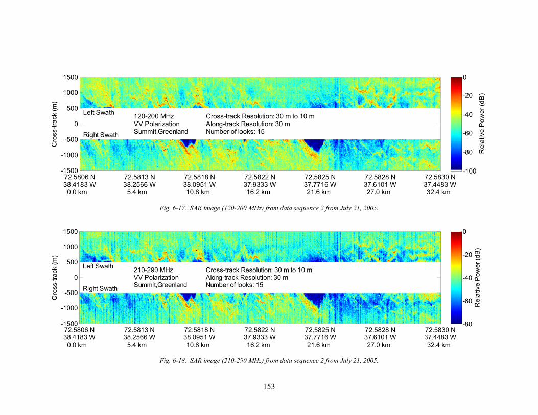
153

72.5806 N38.4183 W

0.0 km

72.5813 N38.2566 W

5.4 km

72.5818 N38.0951 W10.8 km

72.5822 N37.9333 W16.2 km

72.5825 N37.7716 W21.6 km

72.5828 N37.6101 W27.0 km

72.5830 N37.4483 W32.4 km

Cro

ss-tr

ack

(m)



Left Swath

Right Swath

-1500

-1000

-500

0

500

1000

1500

Rel

ativ

e P

ower

(dB

)

-100

-80

-60

-40

-20

0


72.5806 N38.4183 W

0.0 km

72.5813 N38.2566 W

5.4 km

72.5818 N38.0951 W10.8 km

72.5822 N37.9333 W16.2 km

72.5825 N37.7716 W21.6 km

72.5828 N37.6101 W27.0 km

72.5830 N37.4483 W32.4 km

Cro

ss-tr

ack

(m)



Left Swath

Right Swath

-1500

-1000

-500

0

500

1000

1500

Rel

ativ

e P

ower

(dB

)

-80

-60

-40

-20

0


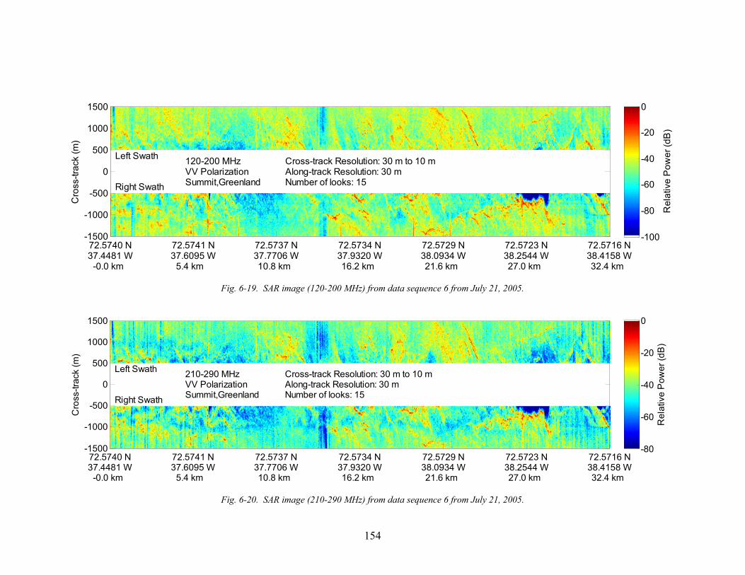
154

72.5740 N37.4481 W

-0.0 km

72.5741 N37.6095 W

5.4 km

72.5737 N37.7706 W10.8 km

72.5734 N37.9320 W16.2 km

72.5729 N38.0934 W21.6 km

72.5723 N38.2544 W27.0 km

72.5716 N38.4158 W32.4 km

Cro

ss-tr

ack

(m)



Left Swath

Right Swath

-1500

-1000

-500

0

500

1000

1500

Rel

ativ

e P

ower

(dB

)

-100

-80

-60

-40

-20

0


72.5740 N37.4481 W

-0.0 km

72.5741 N37.6095 W

5.4 km

72.5737 N37.7706 W10.8 km

72.5734 N37.9320 W16.2 km

72.5729 N38.0934 W21.6 km

72.5723 N38.2544 W27.0 km

72.5716 N38.4158 W32.4 km

Cro

ss-tr

ack

(m)



Left Swath

Right Swath

-1500

-1000

-500

0

500

1000

1500

Rel

ativ

e P

ower

(dB

)

-80

-60

-40

-20

0


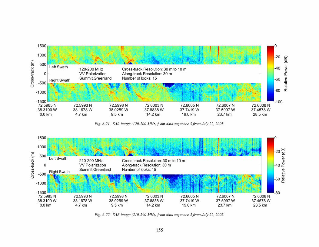
155

72.5985 N38.3100 W

0.0 km

72.5993 N38.1678 W

4.7 km

72.5998 N38.0259 W

9.5 km

72.6003 N37.8838 W14.2 km

72.6005 N37.7419 W19.0 km

72.6007 N37.5997 W23.7 km

72.6008 N37.4578 W28.5 km

Cro

ss-tr

ack

(m)



Left Swath

Right Swath

-1500

-1000

-500

0

500

1000

1500

Rel

ativ

e P

ower

(dB

)

-100

-80

-60

-40

-20

0


72.5985 N38.3100 W

0.0 km

72.5993 N38.1678 W

4.7 km

72.5998 N38.0259 W

9.5 km

72.6003 N37.8838 W14.2 km

72.6005 N37.7419 W19.0 km

72.6007 N37.5997 W23.7 km

72.6008 N37.4578 W28.5 km

Cro

ss-tr

ack

(m)



Left Swath

Right Swath

-1500

-1000

-500

0

500

1000

1500

Rel

ativ

e P

ower

(dB

)

-80

-60

-40

-20

0


156

72.5780 N37.6368 W

0.0 km

72.5780 N37.7659 W

4.3 km

72.5778 N37.8951 W

8.6 km

72.5775 N38.0242 W13.0 km

72.5771 N38.1531 W17.3 km

72.5767 N38.2822 W21.6 km

72.5761 N38.4113 W25.9 km

Cro

ss-tr

ack

(m)



Left Swath

Right Swath

-1500

-1000

-500

0

500

1000

1500

Rel

ativ

e P

ower

(dB

)

-100

-80

-60

-40

-20

0


72.5780 N37.6368 W

0.0 km

72.5780 N37.7659 W

4.3 km

72.5778 N37.8951 W

8.6 km

72.5775 N38.0242 W13.0 km

72.5771 N38.1531 W17.3 km

72.5767 N38.2822 W21.6 km

72.5761 N38.4113 W25.9 km

Cro

ss-tr

ack

(m)



Left Swath

Right Swath

-1500

-1000

-500

0

500

1000

1500

Rel

ativ

e P

ower

(dB

)

-80

-60

-40

-20

0


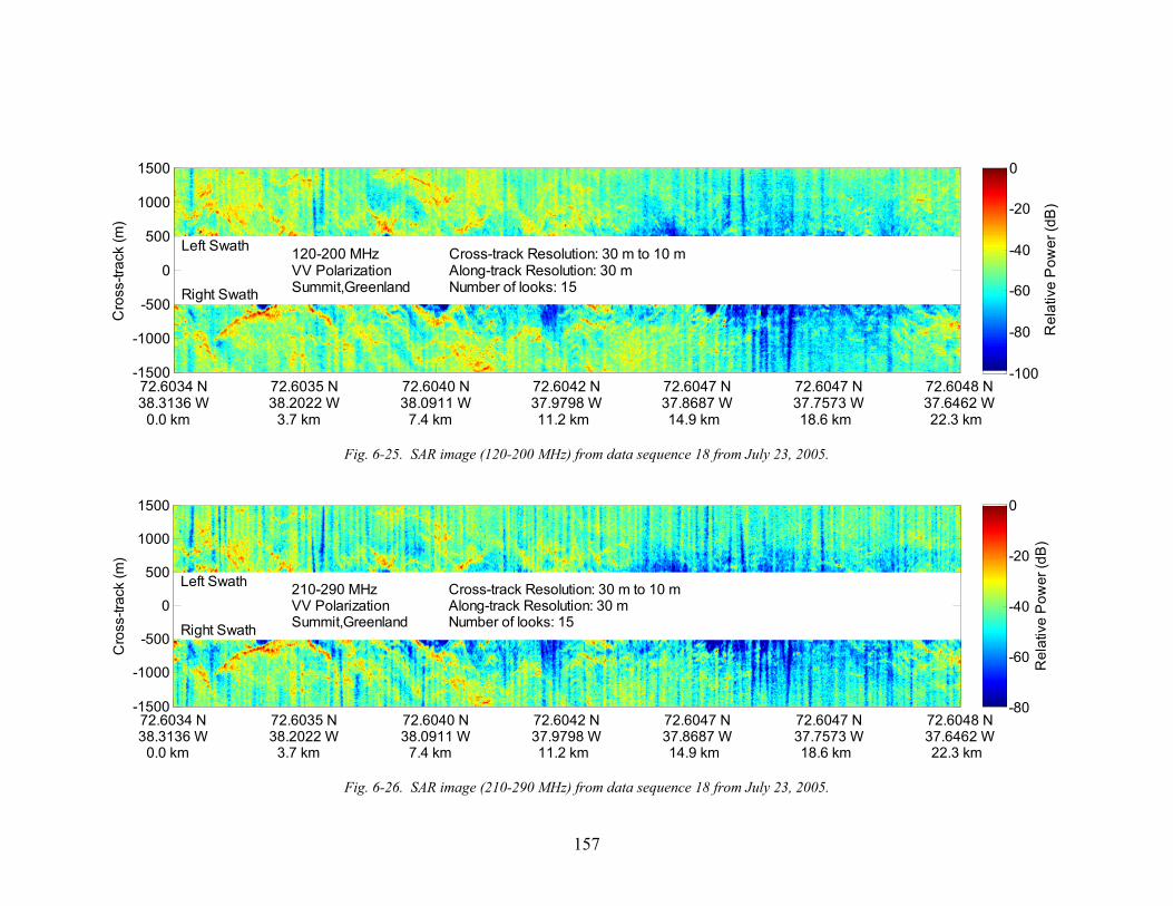
157

72.6034 N38.3136 W

0.0 km

72.6035 N38.2022 W

3.7 km

72.6040 N38.0911 W

7.4 km

72.6042 N37.9798 W11.2 km

72.6047 N37.8687 W14.9 km

72.6047 N37.7573 W18.6 km

72.6048 N37.6462 W22.3 km

Cro

ss-tr

ack

(m)



Left Swath

Right Swath

-1500

-1000

-500

0

500

1000

1500

Rel

ativ

e P

ower

(dB

)

-100

-80

-60

-40

-20

0


72.6034 N38.3136 W

0.0 km

72.6035 N38.2022 W

3.7 km

72.6040 N38.0911 W

7.4 km

72.6042 N37.9798 W11.2 km

72.6047 N37.8687 W14.9 km

72.6047 N37.7573 W18.6 km

72.6048 N37.6462 W22.3 km

Cro

ss-tr

ack

(m)



Left Swath

Right Swath

-1500

-1000

-500

0

500

1000

1500

Rel

ativ

e P

ower

(dB

)

-80

-60

-40

-20

0


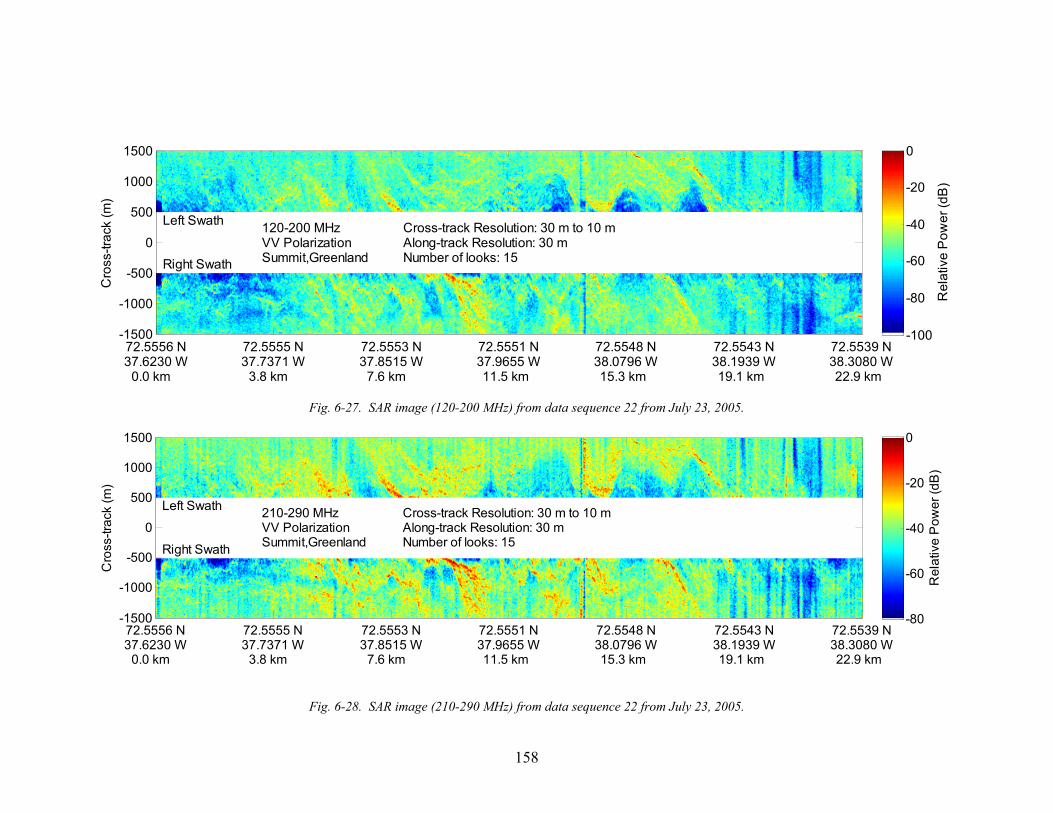
158

72.5556 N37.6230 W

0.0 km

72.5555 N37.7371 W

3.8 km

72.5553 N37.8515 W

7.6 km

72.5551 N37.9655 W11.5 km

72.5548 N38.0796 W15.3 km

72.5543 N38.1939 W19.1 km

72.5539 N38.3080 W22.9 km

Cro

ss-tr

ack

(m)



Left Swath

Right Swath

-1500

-1000

-500

0

500

1000

1500

Rel

ativ

e P

ower

(dB

)

-100

-80

-60

-40

-20

0


72.5556 N37.6230 W

0.0 km

72.5555 N37.7371 W

3.8 km

72.5553 N37.8515 W

7.6 km

72.5551 N37.9655 W11.5 km

72.5548 N38.0796 W15.3 km

72.5543 N38.1939 W19.1 km

72.5539 N38.3080 W22.9 km

Cro

ss-tr

ack

(m)



Left Swath

Right Swath

-1500

-1000

-500

0

500

1000

1500

Rel

ativ

e P

ower

(dB

)

-80

-60

-40

-20

0


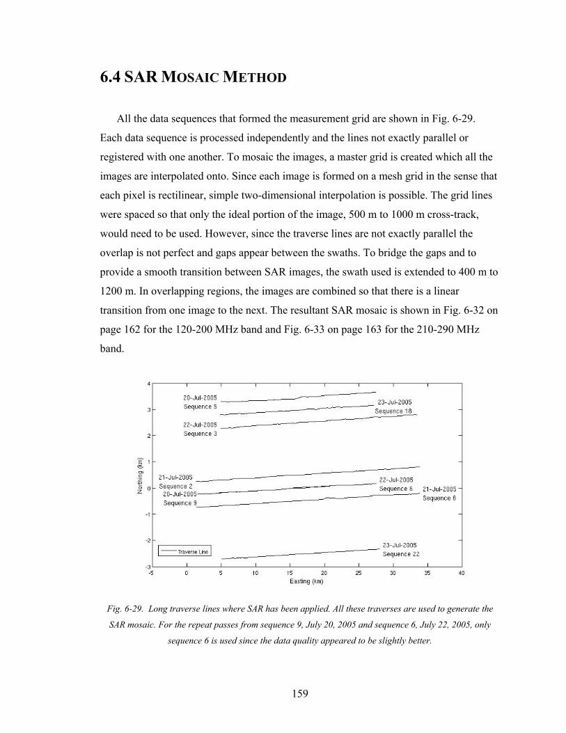
159

6.4 SAR MOSAIC METHOD

All the data sequences that formed the measurement grid are shown in Fig. 6-29.

Each data sequence is processed independently and the lines not exactly parallel or

registered with one another. To mosaic the images, a master grid is created which all the

images are interpolated onto. Since each image is formed on a mesh grid in the sense that

each pixel is rectilinear, simple two-dimensional interpolation is possible. The grid lines

were spaced so that only the ideal portion of the image, 500 m to 1000 m cross-track,

would need to be used. However, since the traverse lines are not exactly parallel the

overlap is not perfect and gaps appear between the swaths. To bridge the gaps and to

provide a smooth transition between SAR images, the swath used is extended to 400 m to

1200 m. In overlapping regions, the images are combined so that there is a linear

transition from one image to the next. The resultant SAR mosaic is shown in Fig. 6-32 on

page 162 for the 120-200 MHz band and Fig. 6-33 on page 163 for the 210-290 MHz

band.

Fig. 6-29. Long traverse lines where SAR has been applied. All these traverses are used to generate the

SAR mosaic. For the repeat passes from sequence 9, July 20, 2005 and sequence 6, July 22, 2005, only

sequence 6 is used since the data quality appeared to be slightly better.

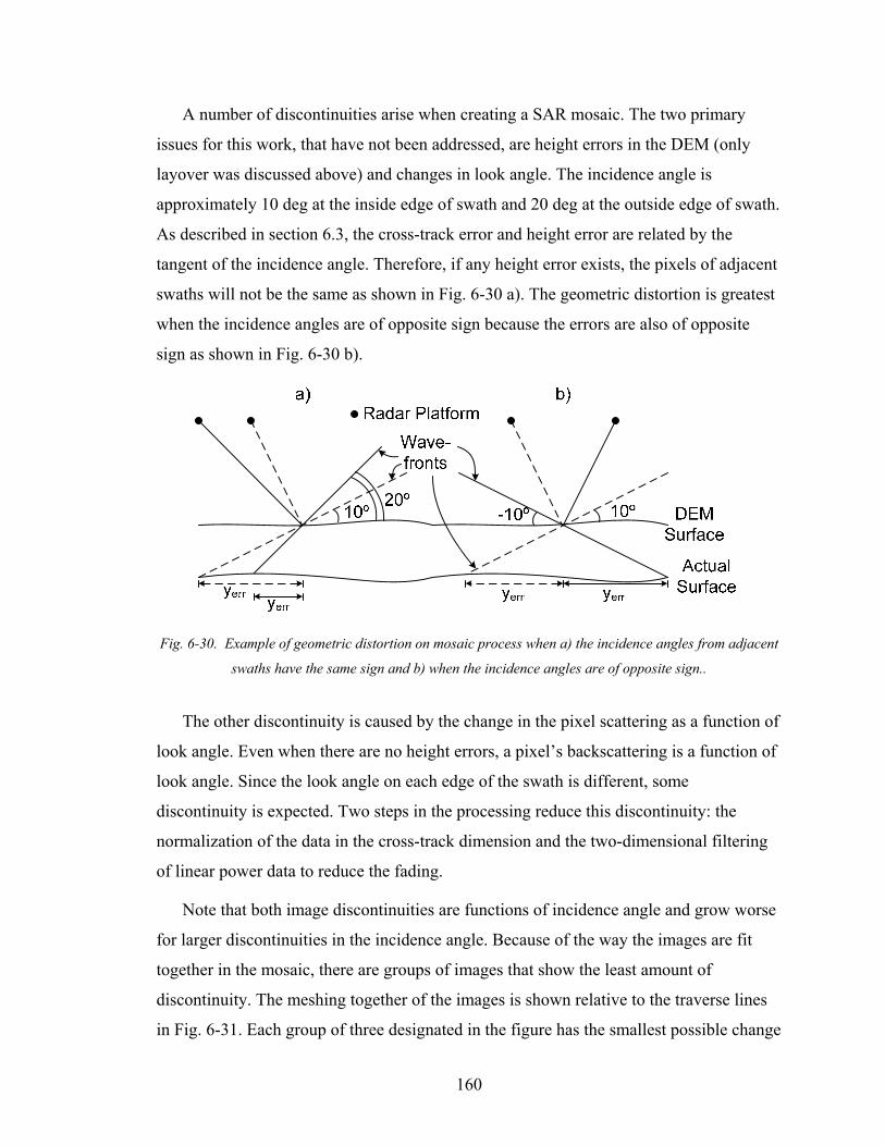
160

A number of discontinuities arise when creating a SAR mosaic. The two primary

issues for this work, that have not been addressed, are height errors in the DEM (only

layover was discussed above) and changes in look angle. The incidence angle is

approximately 10 deg at the inside edge of swath and 20 deg at the outside edge of swath.

As described in section 6.3, the cross-track error and height error are related by the

tangent of the incidence angle. Therefore, if any height error exists, the pixels of adjacent

swaths will not be the same as shown in Fig. 6-30 a). The geometric distortion is greatest

when the incidence angles are of opposite sign because the errors are also of opposite

sign as shown in Fig. 6-30 b).

Fig. 6-30. Example of geometric distortion on mosaic process when a) the incidence angles from adjacent

swaths have the same sign and b) when the incidence angles are of opposite sign..

The other discontinuity is caused by the change in the pixel scattering as a function of

look angle. Even when there are no height errors, a pixel’s backscattering is a function of

look angle. Since the look angle on each edge of the swath is different, some

discontinuity is expected. Two steps in the processing reduce this discontinuity: the

normalization of the data in the cross-track dimension and the two-dimensional filtering

of linear power data to reduce the fading.

Note that both image discontinuities are functions of incidence angle and grow worse

for larger discontinuities in the incidence angle. Because of the way the images are fit

together in the mosaic, there are groups of images that show the least amount of

discontinuity. The meshing together of the images is shown relative to the traverse lines

in Fig. 6-31. Each group of three designated in the figure has the smallest possible change

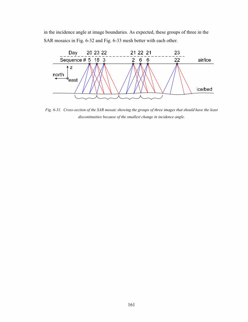
161

in the incidence angle at image boundaries. As expected, these groups of three in the

SAR mosaics in Fig. 6-32 and Fig. 6-33 mesh better with each other.

Fig. 6-31. Cross-section of the SAR mosaic showing the groups of three images that should have the least

discontinuities because of the smallest change in incidence angle.

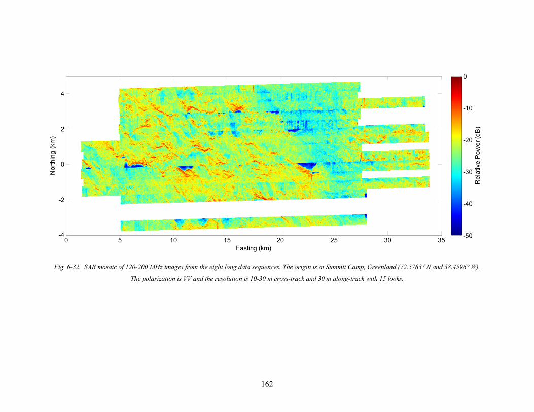
162

Easting (km)

Nor

thin

g (k

m)

0 5 10 15 20 25 30 35-4

-2

0

2

4

Rel

ativ

e P

ower

(dB

)

-50

-40

-30

-20

-10

0

Fig. 6-32. SAR mosaic of 120-200 MHz images from the eight long data sequences. The origin is at Summit Camp, Greenland (72.5783° N and 38.4596° W).

The polarization is VV and the resolution is 10-30 m cross-track and 30 m along-track with 15 looks.

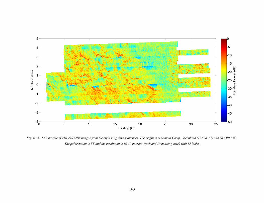
163

Easting (km)

Nor

thin

g (k

m)

0 5 10 15 20 25 30 35-4

-3

-2

-1

0

1

2

3

4

5

Rel

ativ

e P

ower

(dB

)

-50

-45

-40

-35

-30

-25

-20

-15

-10

-5

0

Fig. 6-33. SAR mosaic of 210-290 MHz images from the eight long data sequences. The origin is at Summit Camp, Greenland (72.5783° N and 38.4596° W).

The polarization is VV and the resolution is 10-30 m cross-track and 30 m along-track with 15 looks.

164

Chapter 7: SUMMARY AND RECOMMENDATIONS

7.1 SUMMARY

This work covers the specification, design, development, fielding, and data

processing of a multi-purpose VHF radar for radioglaciological work. The purposes of

the radar are to image the subglacial bed, measure ice thickness, and map deep internal

layers. The ability to form side-looking synthetic aperture radar (SAR) images of the

subglacial bed in thick ice is demonstrated for the first time in this work. The utility of

SAR for terrestrial and oceanic applications is unquestioned. The expansion of SAR into

subglacial imaging brings an extensive set of tools developed for traditional SAR

applications to bear on the glaciological problem of modeling the dynamics of the ice

sheet. Roughness, surface dielectric, and topographic mapping are the primary SAR

applications that address the science objectives outlined in this work. In addition to

imaging, the radar system simultaneously provides a high-resolution ice thickness

estimate and tracks internal layers at depth using a novel multi-waveform approach. Also,

bistatic measurements are possible with the instrument and this configuration has been

tested successfully in the field – although sensitivity-limiting temperature-stability issues

need to be overcome.

In Chapter 2, the propagation model is developed which is used throughout the work.

The propagation model relies on the assumption that the ice sheet may be modeled

locally as a planarly layered media. Since direct measurements of ice properties are

unavailable in the VHF range, we rely on geophysical profiles from nearby ice cores to

model the permittivity of the ice sheet. Using this permittivity profile and previous radar

datasets the required loop sensitivity and dynamic range required by the system to map

deep internal layers and to the image the bed are derived. The f-k migration and SAR

processors also make use of the propagation model as described in Chapter 5 and Chapter

6 respectively.

165

The radar specifications are derived and the system design is covered in Chapter 3.

The final radar specifications pushed the envelope in many ways: broad bandwidth, high-

sensitivity, large-dynamic range, multi-waveform, multi-channel, and bistatic capability.

No previous radar system developed for ice research, has combined all these features into

a single system and this radar system also provided the first multi-waveform approach to

deep penetration ice radars. The broad bandwidth is needed to achieve fine resolution and

map frequency sensitive parameters. The high sensitivity is needed to overcome the

dielectric loss of ice. The large dynamic range is needed to capture the close-specular

internal layers as well as the weak basal scattering. The multi-waveform approach allows

the pulse duration, phase, and radar settings to be changed on a pulse-to-pulse basis

allowing a single radar system to meet all these requirements. The multi-channel

architecture allowed both left and right images to be formed while simultaneously

collecting depth sounder data and solved the wide bandwidth problem caused by antenna

array factor frequency dependence. It also opened the door to more powerful signal

processing techniques such as spectral estimation and minimum mean-squared error

(MMSE) channel combining.

In Chapter 4, the steps in data preconditioning are detailed. The SAR requires

accurate positioning knowledge to reconstruct phase histories. The differential global

positioning system (DGPS) provides the required trajectory information. The setup and

data conditioning are explained including heuristic methods for overcoming poor results

from the kinematic DGPS post-processor. Next, the calibration of the radar and matched

filter processing are described. The calibration method described provides extremely

accurate amplitude and phase accuracy in the measurement. Additional data conditioning

steps to prepare the data for the imaging routines are also covered here. The data indexing

scheme used to organize the data and provide a seamless dataset to the imaging routines

is then described. Finally, a number of methods are tested for re-sampling of the

nonuniform spatial data. It was found that spline interpolation of along-track filtered data

followed by a fast Fourier transform was very efficient computationally and also

provided near-optimal results in terms of the mean squared error criteria.

The f-k migration routine is described in Chapter 5. A number of modifications to the

basic migration method are covered, such as spatial filtering, spatial decimation, time-

166

domain truncation, and nonuniform spatial sampling. The results from the f-k migrated

data show a number of important glaciologically-significant features. These include a

large trench running north and south beside the GRIP bore hole, a bright target in the

bottom of the trench as it passes next to the GRIP site, isolated point targets, and the very

high ice loss near the bed of the ice – significantly higher than predicted by models

derived from laboratory experiments. While the primary purpose of the f-k migration was

to derive the digital elevation map (DEM) for the SAR routine, due to the high sensitivity

of the instrument, a potentially new glaciological feature was uncovered. The layers in

the bottom few hundred meters of the ice sheet appear to be very deformed and to have

lost most of their specular character. The change from specular layers to deformed layers

is rather abrupt and occurs at about 2700-2800 m depth. In the 25-50 m next to the bed

the deformed layers all but disappear. This may provide a link to why the GRIP and

GISP2 cores are highly correlated along their whole lengths until they reach this region of

the ice.

In Chapter 6, a time domain correlation SAR processor is used to form the images.

The reason for working in the space-time domain is because it allows complete flexibility

in both antenna and target positioning which traditional frequency domain techniques do

not allow. Due to the short range and small incidence angles in the system geometry, the

use of a conformally mapped target distribution is necessary for generating images. It is

also important to include the height in the target distribution when creating a mosaic of

images because height estimation errors during the meshing processes cause

discontinuities. Additionally, because of the cross-track meandering of the platform,

motion compensation required for frequency-domain methods would have been very

difficult to apply without deteriorating the image quality. The SAR results are presented

for two different subbands: 120-200 and 210-290 MHz. Both simulated and measured

results show that left-right ambiguity and SNR are not an issue across the scene. The

SAR mosaic shows that the images can be fused together successfully into a mosaic,

although height errors in the DEM mean that some images with significantly different

look angles do not match up as well.

Although the primary missions of this work were successful, several failures occurred

and lessons were learned from the experience. Also, recommendations for future work

167

with the dataset are worth noting. The final portion of this chapter, attempts to cover

these final topics.

7.2 RADAR SYSTEM IMPROVEMENTS

A number of hardware related problems and limitations are described in this section.

Some of these problems occurred during the first field season and were fixed for the

second field season. Others would have required a large expense to fix, but were taken as

lessons learned that should be incorporated into future systems.

During the first field season, we had two hardware failures. Both were fixed for the

second field season and no further problems were found. The first failure happened

during the field calibration: both high-power transmit amplifier switches failed and only

one backup was available. Because of this, the system was operated without transmit

antenna switching which reduced the cross-track resolution by two. The switches had

been tested extensively in the laboratory. When returned to the manufacturer, faulty

isolation between the control circuitry and the high power RF path were blamed. A

different manufacturer was used for the replacement switches.

The second failure had to do with vibration-induced noise. Later in the laboratory, it

was found that the multiplexer and voltage regulators were not properly isolated through

the DC bias. We suspect that the multiplexer’s biasing was affected by low-frequency

signals from the voltage regulator. Insertion of another DC-block capacitor and a 3 dB

attenuator fixed the problem. Although not thoroughly tested, we think the vibrations

during vehicle movement or upsetting the cables may have occasionally disrupted the DC

path which set-off the noise. We suspect that the use of SMA connectors was not a good

choice due to the exposure and the weight and size of the low-loss cables. Subsequent

analysis of the noise showed that it occurred as spurs in the frequency domain.

Fortunately, this allowed for automated suppression of the noise with only moderate

degradation of the radar performance. First a detection routine was created which

detected the presence of noise spikes and then the offending frequency bins were set to

zero. Fig. 6-1 shows a SAR image before and after correction.

168

Fig. 7-1. SAR image a) before and b) after removal of noise spurs. The noise spurs show up as bright red

vertical lines in a).

During the first field season of the radar system, we ran into electromagnetic

interference (EMI) problems with the bistatic measurements due to a small separation

between the system and the receive antenna. Even though the radar system is enclosed in

a commercial ruggedized EMI box – significant signal power was able to couple into the

receive antenna. This was validated in the RF-quiet Sprint anechoic chamber by

169

operating with the receive antenna and system inside the chamber and with just the

antenna in the chamber. With just the antenna in the chamber, the measured noise floor

matched the thermal noise floor. With the system and antenna in the chamber, the noise

floor was 10 dB higher and contained both coherent and incoherent components. The

coherent component is particularly problematic because even with the long-dwell times

possible with ground-work, this energy can not be removed unless it is coherent over

long periods of time. Given the nature of EMI and the drift in the bistatic receiver’s

stable local oscillator (STALO) relative to the transmitter’s STALO, removal of the noise

is a nontrivial task. For future operations, special attention should be paid to unintentional

coupling of signal power into the receive antennas. In our case, we simply increased the

separation between the receive antenna and the system.

During the second field season, the extreme cold and variations in temperature caused

locking issues with the bistatic system. A temperature-stable system would not only solve

the bistatic system’s problem, but would also provide more accurate results in general.

Plus it would alleviate the time-consuming process of checking the phase stability of the

high speed data acquisition system before and after measurements every day and the

arduous task of trying to keep the cabin-temperature stable during measurements.

All external connectors are SMA. Due to vibrations, the physical size and weight of

low-loss cables, and the difficulty of working with small connectors in the cold, all

external connectors should be replaced with Type-N connectors. As mentioned in the

preceding paragraph, the SMA connectors may have also contributed to the vibration-

induced noise spurs. Aside from greatly improved mechanical performance, Type-N

connectors can also carry more RF power which would allow the system’s power

amplifiers to be upgraded without having to replace the antenna feed network.

The post-processed DGPS data had many errors in them. An in-house algorithm was

used to partially circumvent these errors, but is a less than satisfactory solution. Limited

testing of the DGPS system before the field experiment and in the field before the

traverse runs showed no problems. We suspect that the mounting structure for the DGPS

antennas may have been responsible for the problems. The antennas were mounted on

masts as shown in Fig. 3-18. This mounting technique was problematic because the masts

170

vibrated constantly during platform movement which may have contributed to problems

with the post-processing. This hypothesis has not been tested however and is left as

future work. Although possibly cost prohibitive, other manufacturers such as Ashtech

may be more appropriate for kinematic work (e.g. the Jet Propulsion Laboratory uses

Ashtech).

7.3 COMMON MID-POINT (CMP) MEASUREMENTS

Common mid-point (CMP)22 measurements on an ice sheet measure scattered energy

from a common reflecting layer along different propagation paths as shown in Fig 7-2a.

An estimate of velocity and attenuation can be determined by monitoring the behavior of

the scattered energy from the layer as a function of the transmitter and receiver baseline.

The permittivity of the ice sheet changes continuously with depth, so reflecting horizons

at many depths are required to adequately determine the profile. Fortunately, there are

detectable layers starting from the air/ice interface down to the bed, which can be used

for permittivity calculations. Because ice is a low loss material (i.e. dielectric), the

problem of estimating the permittivity can be divided into two separate problems: one of

estimating the real permittivity via the velocity [145], [146], [147], [148], [149], [150]

and one of estimating the imaginary part by the attenuation [151], [152].

Offset (m)

Two-

Way

Tra

vel T

ime

(ns)

0 2 4 6 8 10

0

20

40

60

80

100

120

140

160

Fig 7-2. a) Illustration of common midpoint geometry. b) Idealized radar dataset using a Gaussian

impulse for the transmit waveform with 1 m range resolution, depth to interface of 10 m, and 78.1' =ε .

22 Also known as common depth point (CDP) or wide-angle measurements.

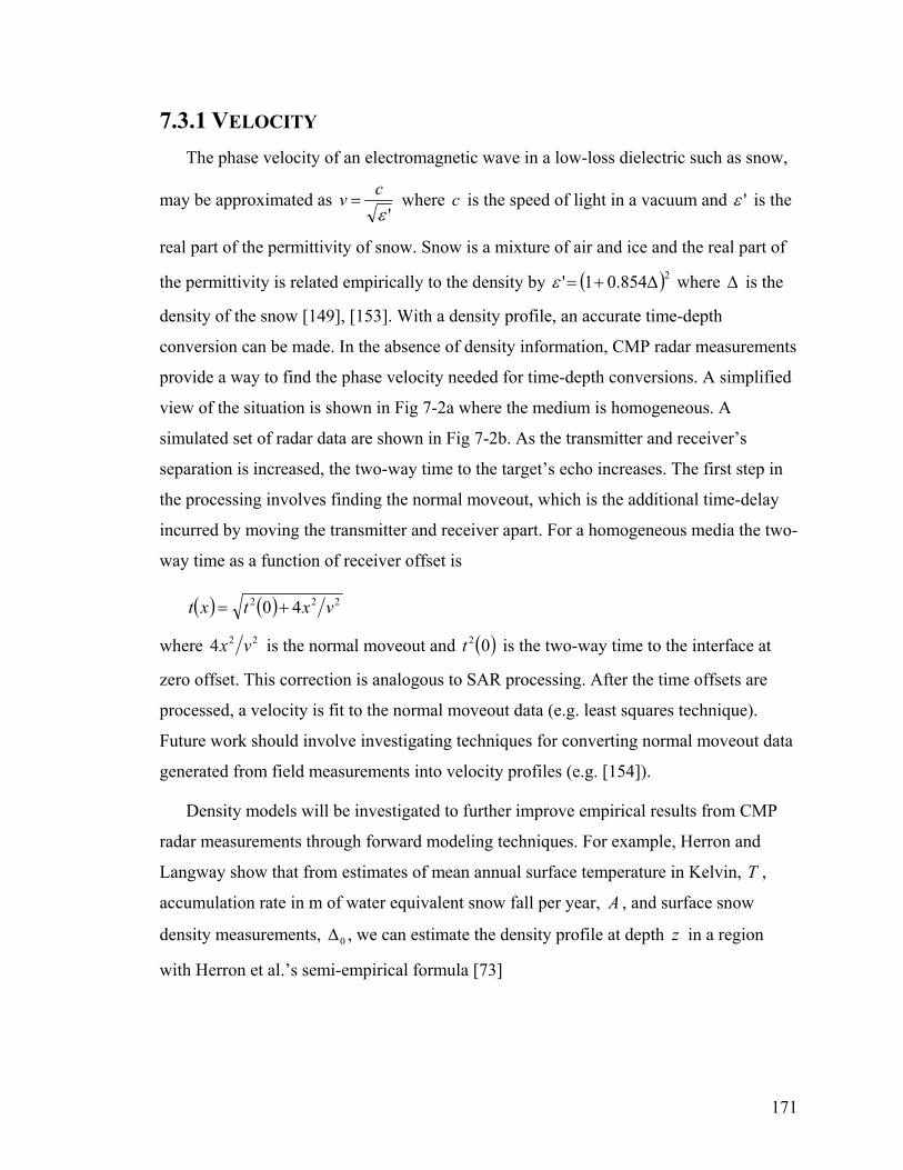
171

7.3.1 VELOCITY The phase velocity of an electromagnetic wave in a low-loss dielectric such as snow,

may be approximated as 'ε

cv = where c is the speed of light in a vacuum and 'ε is the

real part of the permittivity of snow. Snow is a mixture of air and ice and the real part of

the permittivity is related empirically to the density by ( )2854.01' ∆+=ε where ∆ is the

density of the snow [149], [153]. With a density profile, an accurate time-depth

conversion can be made. In the absence of density information, CMP radar measurements

provide a way to find the phase velocity needed for time-depth conversions. A simplified

view of the situation is shown in Fig 7-2a where the medium is homogeneous. A

simulated set of radar data are shown in Fig 7-2b. As the transmitter and receiver’s

separation is increased, the two-way time to the target’s echo increases. The first step in

the processing involves finding the normal moveout, which is the additional time-delay

incurred by moving the transmitter and receiver apart. For a homogeneous media the two-

way time as a function of receiver offset is

( ) ( ) 222 40 vxtxt +=

where 224 vx is the normal moveout and ( )02t is the two-way time to the interface at

zero offset. This correction is analogous to SAR processing. After the time offsets are

processed, a velocity is fit to the normal moveout data (e.g. least squares technique).

Future work should involve investigating techniques for converting normal moveout data

generated from field measurements into velocity profiles (e.g. [154]).

Density models will be investigated to further improve empirical results from CMP

radar measurements through forward modeling techniques. For example, Herron and

Langway show that from estimates of mean annual surface temperature in Kelvin, T ,

accumulation rate in m of water equivalent snow fall per year, A , and surface snow

density measurements, 0∆ , we can estimate the density profile at depth z in a region

with Herron et al.’s semi-empirical formula [73]

172

( )( )

( )

∆≥∆Ζ+Ζ∆

∆<∆Ζ+Ζ∆

=∆c

i

ci

z

zz

1

1

0

0

1

1

where

3i cmg917.0 ⋅=∆ is the density of pure ice,

3c cmg55.0 ⋅=∆ is the critical density where the form of ( )z∆ changes,

( ) [ ]0000 lnexp ∆−∆∆+∆=Ζ ii zk ,

( ) [ ]cici Azk ∆−∆∆+∆=Ζ lnexp 5.011 ,

⋅−=

−

RTk

1

0Jmol10160exp11 ,

⋅−=

−

RTk

1

1Jmol21400exp575 ,

and

11 molKJ314.8 −− ⋅⋅=R is the universal gas constant.

7.3.2 ATTENUATION Assuming specular reflections from internal layers, we can use the specular radar

equation to model the power received from a layer as a function of radar offset:

( ) ( ) ( )( )

( ) 2223

2

,,64

,,,,ppttt

tice

rrrttttr RfL

RfncfGfGfPP Γ= θ

πφθφθ .

Assuming accurate knowledge of the transmit power, gain, and range; the only two

unknowns are the dielectric loss and Fresnel reflection coefficient. The reflection

coefficient is, however, a weak function of the offset position when the incidence angle is

small. To demonstrate this, the power reflection coefficient versus receiver offset from a

typical internal layer at 500 m depth is shown in Fig 7-3. Therefore, by monitoring power

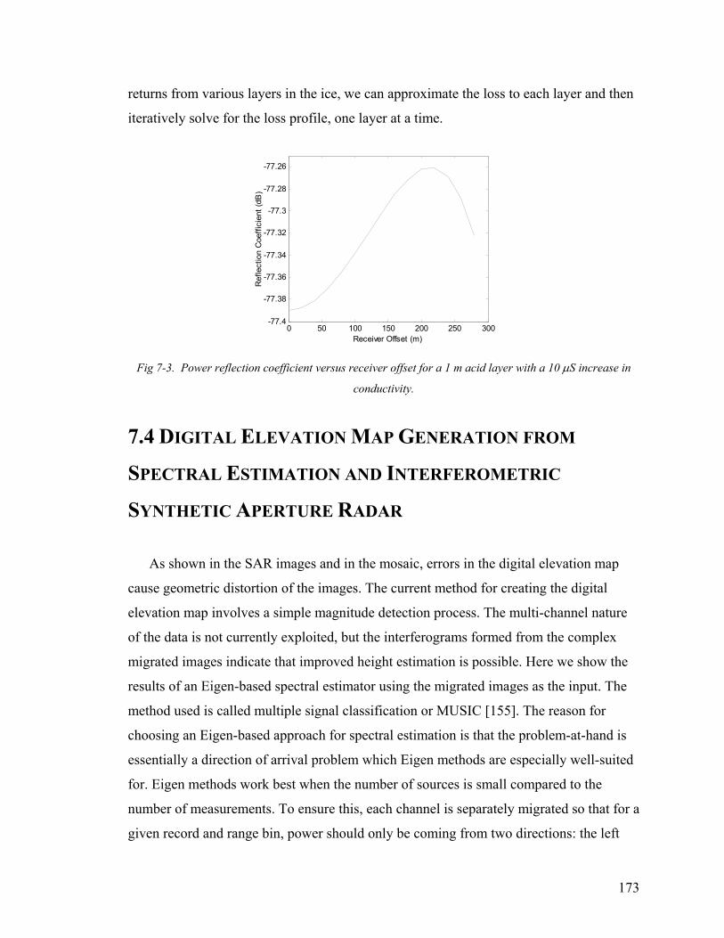
173

returns from various layers in the ice, we can approximate the loss to each layer and then

iteratively solve for the loss profile, one layer at a time.

0 50 100 150 200 250 300-77.4

-77.38

-77.36

-77.34

-77.32

-77.3

-77.28

-77.26

Receiver Offset (m)

Ref

lect

ion

Coe

ffici

ent (

dB)

Fig 7-3. Power reflection coefficient versus receiver offset for a 1 m acid layer with a 10 µS increase in

conductivity.

7.4 DIGITAL ELEVATION MAP GENERATION FROM

SPECTRAL ESTIMATION AND INTERFEROMETRIC

SYNTHETIC APERTURE RADAR

As shown in the SAR images and in the mosaic, errors in the digital elevation map

cause geometric distortion of the images. The current method for creating the digital

elevation map involves a simple magnitude detection process. The multi-channel nature

of the data is not currently exploited, but the interferograms formed from the complex

migrated images indicate that improved height estimation is possible. Here we show the

results of an Eigen-based spectral estimator using the migrated images as the input. The

method used is called multiple signal classification or MUSIC [155]. The reason for

choosing an Eigen-based approach for spectral estimation is that the problem-at-hand is

essentially a direction of arrival problem which Eigen methods are especially well-suited

for. Eigen methods work best when the number of sources is small compared to the

number of measurements. To ensure this, each channel is separately migrated so that for a

given record and range bin, power should only be coming from two directions: the left

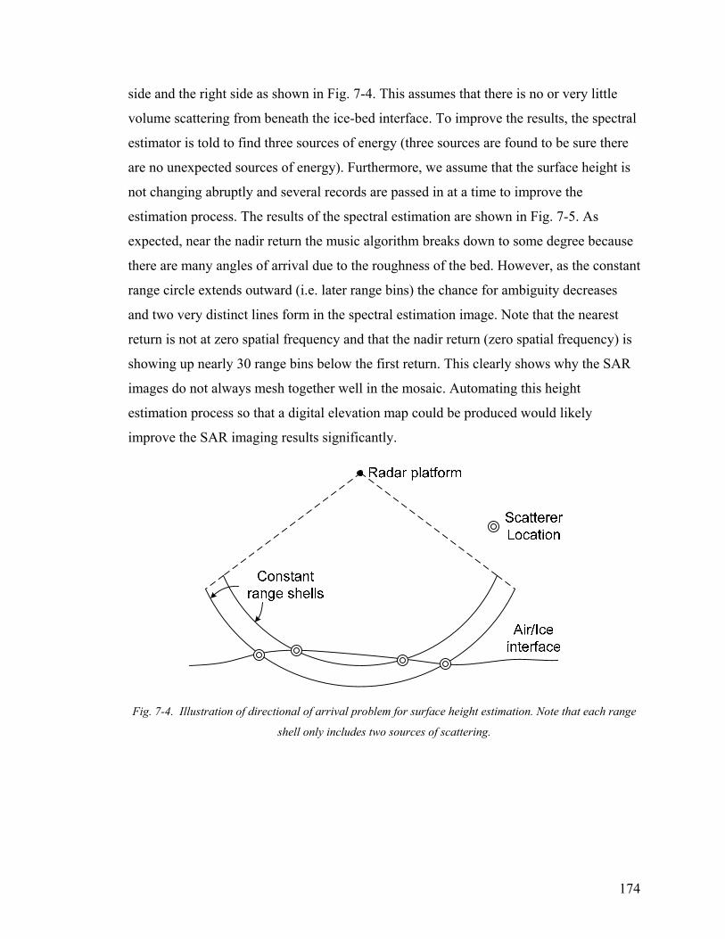
174

side and the right side as shown in Fig. 7-4. This assumes that there is no or very little

volume scattering from beneath the ice-bed interface. To improve the results, the spectral

estimator is told to find three sources of energy (three sources are found to be sure there

are no unexpected sources of energy). Furthermore, we assume that the surface height is

not changing abruptly and several records are passed in at a time to improve the

estimation process. The results of the spectral estimation are shown in Fig. 7-5. As

expected, near the nadir return the music algorithm breaks down to some degree because

there are many angles of arrival due to the roughness of the bed. However, as the constant

range circle extends outward (i.e. later range bins) the chance for ambiguity decreases

and two very distinct lines form in the spectral estimation image. Note that the nearest

return is not at zero spatial frequency and that the nadir return (zero spatial frequency) is

showing up nearly 30 range bins below the first return. This clearly shows why the SAR

images do not always mesh together well in the mosaic. Automating this height

estimation process so that a digital elevation map could be produced would likely

improve the SAR imaging results significantly.

Fig. 7-4. Illustration of directional of arrival problem for surface height estimation. Note that each range

shell only includes two sources of scattering.

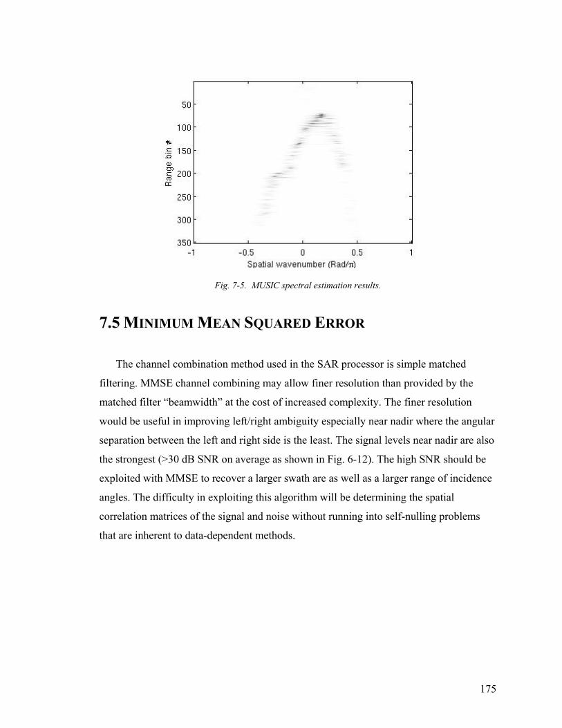
175

Fig. 7-5. MUSIC spectral estimation results.

7.5 MINIMUM MEAN SQUARED ERROR

The channel combination method used in the SAR processor is simple matched

filtering. MMSE channel combining may allow finer resolution than provided by the

matched filter “beamwidth” at the cost of increased complexity. The finer resolution

would be useful in improving left/right ambiguity especially near nadir where the angular

separation between the left and right side is the least. The signal levels near nadir are also

the strongest (>30 dB SNR on average as shown in Fig. 6-12). The high SNR should be

exploited with MMSE to recover a larger swath are as well as a larger range of incidence

angles. The difficulty in exploiting this algorithm will be determining the spatial

correlation matrices of the signal and noise without running into self-nulling problems

that are inherent to data-dependent methods.

176

REFERENCES

[1] Douglas, Bruce C., Michael S. Kearney, and Stephen P. Leatherman, Sea Level

Rise: History and Consequences, International Geophysics Series Vol. 75,

Academic Press, San Diego, 2001.

[2] Douglas, Bruce C., and W. Richard Peltier, “The puzzle of global sea-level rise,”

Physics Today, pp. 35-40, March 2002.

[3] IPCC, Climate Change 2001: The Scientific Basis, IPCC, Geneva, Switzerland,

2001.

[4] IPCC, Climate Change 2001: The Scientific Basis, IPCC, Geneva, Switzerland,

2001, pg 26.

[5] Waggoner, Paul E., Climate Changes and U.S. Water Resources, John Wiley and

Sons, New York, 1990.

[6] Rignot, Eric and Robert H. Thomas, “Mass Balance of Polar Ice Sheets,” Science,

vol 297, pp. 1502-1506, 30 August 2002.

[7] Terence J. Hughes, Ice Sheets, Oxford University Press, New York, 1998.

[8] Houghton, J. T., B. A. Callander, and S. K. Varney. The 1992 IPCC Supplement:

Scientific Assessment. In Climate Change 1992: The Supplementary Report to the

IPCC Scientific Assessment, Cambridge University Press, Cambridge, England,

1992.

[9] Nesje, Atle and Svein Olaf Dahl, Glaciers and Environmental Change, pp 48,

Oxford University Press, New York, 2000.

[10] NASA Ocean and Ice Branch, http://neptune.gsfc.nasa.gov/moceansice.html,

Chester J. Koblinsky, March 2003.

[11] NASA Earth Science Enterprise,

http://www.earth.nasa.gov/visions/researchstrat/Research_Strategy.htm,

“Understanding earth system change NASA’s Earth science enterprise research

strategy for 2000-2010”, NASA Earth Systems Science Research Strategy,

October 2001.

177

[12] Van der Veen, Cornelis J., Fundamentals of Glacier Dynamics, A. A. Balkema,

Rotterdam, Netherlands, 1999.

[13] Krabill, William B., Waleed Abdalati, Earl Frederick, Serdar Manizade, Chreston

Martin, John G. Sonntag, Robert N. Swift, Robert H. Thomas, W. Wright, J.

Yungel, “Greenland ice sheet: high elevation balance and peripheral thinning,”

Science, vol 289, no 5478, pp. 428-430, 21 July 2000.

[14] Kanagaratnam, Pannir, Silvaprasad Gogineni, Niels Gundestrup, and Lars Larsen,

“High-resolution radar mapping of internal layers at the North Greenland Ice Core

Project”, Journal of Geophysical Research, vol 106, no. D24, pp. 33799-33811,

Dec 27, 2001.

[15] Gogineni, Silvaprasad, Dilip Tammana, David Braaten, Carl Leuschen, Torry

Akins, Justin Legarsky, Pannir Kanagaratnam, Jim Stiles, Christopher T. Allen,

and Kenneth C. Jezek, “Coherent radar ice thickness measurement over the

Greenland ice sheet”, Journal of Geophysical Research, vol 106, no. D24, pp.

33761-33772, Dec 27, 2001.

[16] Bamber, Jonathan L., Russell L. Layberry and Silvaprasad Gogineni, “A new ice

thickness and bed data set for the Greenland ice sheet, 1. Measurement, data

reduction, and errors”, Journal of Geophysical Research, vol 106, no. D24, pp.

33773-33780, Dec 27, 2001.

[17] Arendt, Anthony A., Keith A. Echelmeyer, William D. Harrison, Craig S. Lingle,

and Virginia B. Valentine, “Rapid wastage of Alaska glaciers and their

contribution to rising sea level,” Science, vol 297, pp. 382-386, 19 July 2002.

[18] Bentley, Charles R., N. Lord, C. Liu, “Radar reflections reveal a wet bed beneath

stagnant ice stream C and a frozen bed beneath ridge BC, West Antarctica,”

Journal of Glaciology, vol. 44, no. 146, 1998, pp. 149-156.

[19] Gades, Anthony M., Charles F. Raymond, Howard B. Conway, and Robert W.

Jacobel, “Bed properties of Siple Dome and adjacent ice streams, West

Antarctica, inferred from radio-echo sounding measurements,” Journal of

Glaciology, vol .46, no. 152, 2000, pp. 88-94.

178

[20] Gades, Anthony M., “Spatial and temporal variations of basal conditions beneath

glaciers and ice sheets inferred from radio echo-sounding measurements,” Ph. D.

Thesis, University of Washington, 1998.

[21] Ohmae, Hirokazu, Fumihiko Nishio, and Shinji Mae, “Distribution of reflected

power from the bed by radio echo-sounding in the Shirase Glacier drainage area,

East Dronning Maud Land, Antarctica,” Annals of Glaciology, vol. 12, 1989, pp.

124-126.

[22] Neal, C. S., “The dynamics of the Ross Ice Shelf revealed by radio echo-

sounding,” Journal of Glaciology, vol. 24, no. 90, 1979, pp. 295-307.

[23] Winebrenner, Dale P., Benjamin E. Smith, Ginny A. Catania, Howard B.

Conway, Charles F. Raymond, “Radio-frequency attenuation beneath Siple

Dome, West Antarctica, from wide-angle and profiling radar observations,”

Annals of Glaciology, vol. 37, 2003, pp. 226-232.

[24] Allen, Chris T., M. Gandhi, Silvaprasad Gogineni, and Kenneth C. Jezek,

“Feasibility study for mapping the polar ice bottom topography using

interferometric synthetic-aperture radar techniques,” RSL Technical Report

11680-1, 1997.

[25] Neal, C. S., “Radio echo determination of basal roughness characteristics on the

Ross Ice Shelf,” Annals of Glaciology, vol. 3, 1982, pp. 216-221.

[26] Oswald, Gordon K. A., “Investigation of sub-ice bedrock characteristics by radio-

echo sounding,” Journal of Glaciology, vol. 15, no. 73, 1975, pp. 75-87.

[27] Peters, Matthew E., Donald D. Blankenship, and David L. Morse, “Analysis

techniques for coherent airborne radar sounding: application to West Antarctica

ice streams,” Journal of Geophysical Research, vol. 110, 9 Jun 2005, B06303,

doi:10.1029/2004JB003222.

[28] Retzlaff, R., N. Lord, and Charles R. Bentley, “Airborne-radar studies: ice

streams A, B, and C, West Antarctica,” Journal of Glaciology, vol. 39, no. 133,

1993.

[29] Shabtaie, Sion, Ian M. Whillans, Charles R. Bentley, “The morphology of ice

streams A, B, and C, West Antarctica, and their environs,” Journal of

Geophysical Research, vol. 92, no. B9, 10 Aug 1987, pp. 8865-8883.

179

[30] Rose, K. E., “Characteristics of ice flow in Marie Byrd Land, Antarctica,” Journal

of Glaciology, vol. 24, 1979, pp. 63-75.

[31] Englehardt, Hermann, Neil Humphrey, and Barclay Kamb, “Borehole geophysical

observations on ice stream B, Antarctica,” Antarctic Journal, vol. 25, no. 5, 1990,

pp. 80-82.

[32] Blankenship, Donald D., Charles R. Bentley, S. T. Rooney, and Richard B. Alley,

“Till beneath ice stream B 1. Properties derived from seismic travel times,”

Journal of Geophysical Research, vol. 92, no. B9, Aug 10, 1987, pp. 8903-8911.

[33] Alley, Richard B., Donald D. Blankenship, Charles R. Bentley, and S. T. Rooney,

“Deformation of till beneath ice stream B, West Antarctica,” Nature, vol 322, Jul

3, 1986, pp. 57-59.

[34] Barclay Kamb, “Basal zone of the west Antarctic ice streams and its role in

lubrication of their rapid motion,” in The West Antarctic Ice Sheet: Behavior and

Environment, Antarctic Research Series, vol. 77, American Geophysical Union,

Washington, D.C., 2001, pp. 157-199.

[35] Paterson, W. S. B., The Physics of Glaciers, Third Edition, Butterworth-

Heinemann, Jordan Hill, Oxford, 1998, pp. 301.

[36] Fahnestock, Mark, Robert Bindschadler, Ron Kwok, and Ken Charles Jezek,

“Greenland ice sheet surface properties and ice dynamics from ERS-1 SAR

imagery,” Science, vol. 262, no. 5139, 3 Dec 1993, pp. 1530-1534.

[37] Joughin, Ian, Laurence Gray, Robert Bindschadler, Stephen Price, David Morse,

Christina Hulbe, Karim Mattar, Charles Werner, “Tributaries of West Antarctic

ice streams revealed by RADARSAT interferometry,” Science, vol. 286, no.

5438, 8 Oct 1999, pp. 283-286.


Heinemann, Jordan Hill, Oxford, 1998, pp. 140-2.


Heinemann, Jordan Hill, Oxford, 1998, Chapter 7.



180



[42] Jezek, Kenneth C., Personal Communication, Oct 1, 2005.

[43] Gogineni, Silvaprasad, “A mobile sensor web for polar ice sheet measurements,”

NSF Proposal, October 2001.

[44] Schoof, Christian, “Basal perturbations under ice streams: form drag and surface

expression,” Journal of Glaciology, vol. 48, no. 162, 2002, pp. 407-416.

[45] Dahl-Jensen, Dorthe, “Enhanced: The Greenland Ice Sheet Reacts,” Science, vol.

289, no. 5478, 21 July 2000, pp. 404-5.

[46] Dahl-Jensen, Dorthe, Niels S. Gundestrup, Siva Prasad Gogineni, Heinz Miller,

“Basal melt at NorthGRIP modeled from borehole, ice-core and radio-echo

sounder observations,” Annals of Glaciology, vol. 37, 2003, pp. 207-212.

[47] Englehardt, Hermann and Barclay Kamb, “Basal hydraulic system of a West

Antarctica ice stream: constraints from borehole observations,” Journal of

Glaciology, vol 43, no 144, pp 207-229, 1998.

[48] Anandakrishnan, Sridhar, personal communication, Sept 30, 2005.

[49] Anandakrishnan, Sridhar, Richard B. Alley, Robert W. Jacobel, and Howard

Conway, “The flow regime of ice stream C and hypothesis concerning its recent

stagnation,” in The West Antarctic Ice Sheet: Behavior and Environment,

Antarctic Research Series, vol. 77, American Geophysical Union, Washington,

D.C., 2001, pp. 283-294.

[50] Gogineni, Silvaprasad, “Center for Remote Sensing of Ice Sheets,” NSF Proposal,

October 2004.

[51] Parthasarathy, Rohit, “Fine-resolution radar for near-surface layer mapping,”

M.S. Thesis, University of Kansas, Aug. 25, 2004.

[52] Clow, Gary D., R. W. Saltus, and E. D. Waddington, “A new high-precision

borehole-temperature logging system used at GISP2, Greenland, and Taylor

Dome, Antarctica,” Journal of Glaciology, vol. 42, 1996, pp. 576-584.

[53] Gow, Anthony J. and Debra A. Meese, "Nature of basal debris in the GISP2 and

Byrd ice cores and its relevance to bed processes," Annals of Glaciology, vol. 22,

1996, pp 134-140.

181

[54] Harrison, C. H., Radio echo sounding of horizontal layers in ice,” Journal of

Glaciology, vol. 12, no. 66, 1973, pp. 383-397.

[55] Fujita, Shuji, Takeshi Matsuoka, Toshihiro Ishida, Kenichi Matsuoka, and Shinji

Mae, “A summary of the complex dielectric permittivity of ice in the megahertz

range and its application for radar sounding of polar ice sheets,” Physics of Ice

Core Records, Edited by T. Hondoh, Hokkaido University Press, 2000, Sapporo,

pp. 185-212.

[56] E. Wolff, J. Moore, H. Clausen, C. Hammer, J. Kipfstuhl, and K. Fuhrer, “Long-

term changes in the acid and salt concentrations of the Greenland Ice Core Project

ice core from electrical stratigraphy,” Journal of Geophysical Research, vol. 100,

no. D8, pp. 16249-16263, Aug. 20, 1995. Data archived at the World Data Center

for Paleoclimatology, Boulder, Colorado, USA.

[57] J. Bolzan and M. Strobel, “Accumulation-rate variations around Summit,

Greenland,” Journal of Glaciology, vol. 40, pp. 56-66, 1994. Data archived at the

World Data Center for Paleoclimatology, Boulder, Colorado, USA.

[58] Twickler, Mark, personal communication, Aug. 30, 2004.

[59] Kanagaratnam, Pannirselvam, “Airborne radar for high-resolution mapping of

internal layers in glacial ice to estimate accumulation rate,” Ph. D. Thesis,

University of Kansas, 2002.

[60] Paden, John D., Christopher T. Allen, Sivaprasad Gogineni, Kenneth Charles

Jezek, Dorthe Dahl-Jensen, Lars B. Larsen, “Wideband measurements of ice sheet

attenuation and basal scattering,” IEEE Geoscience and Remote Sensing Letters,

vol. 2, no. 2, Apr 2005, pp. 164-168.

[61] Matzler, Christian and Urs Wegmuller, “Dielectric properties of fresh-water ice at

microwave frequencies,” Journal of Physics D: Applied Physics, vol. 20, 1987,

pp. 1623-1630.

[62] Matsuoka, Takeshi, Shuji Fujita, and Shinji Mae, “Effect of temperature on

dielectric properties of ice in the range 5-39 GHz,” Journal of Applied Physics,

vol. 80, no. 10, 15 Nov 1996, pp. 5884-5890.

[63] Wolff, Eric W., John C. Moore, Henrik B. Clausen, Claus U. Hammer, Josef

Kipfstuhl, and Katrin Fuhrer, “Long-term changes in the acid and salt

182

concentrations of the Greenland Ice Core Project ice core from electrical

stratigraphy,” Journal of Geophysical Research, vol. 100, no. D8, 20 Aug 1995,

pp. 16249-16263.

[64] Corr, Hugh F J, John C Moore, and Keith W. Nicholls, “Radar absorption due to

impurities in Antarctic ice,” Geophysical Research Letters, vol. 20, no. 11, pp.

1071-1074, Jun 7, 1993.

[65] Tiuri, Martti E., Ari H. Sihvola, Ebbe G. Nyfors, Martti T. Hallikaiken, “The

complex dielectric constant of snow at microwave frequencies,” IEEE Journal of

Oceanic Engineering, vol. OE-9, no. 5, Dec 1984, pp. 377-382.

[66] Berizzi, F., G. Corsini, M. Diani, M. Veltroni, “Autofocus of wide azimuth angle

SAR images by contrast optimization,” IEEE Conference on Acoustics, Speech,

and Signal Processing (ICASSP) , Albequerque, NM, 3-6 Apr 1990, pp. 1230-

1232.

[67] Elachi, Charles, Spaceborne Radar Remote Sensing: Applications and

Techniques, Institute of Electrical and Electronics Engineers, New York, NY,

1988, pp. 144-145.

[68] Green, J. F. and C. J. Oliver, “The limits on autofocus accuracy in SAR,”

International Journal of Remote Sensing, vol. 13, no. 14, 1992, pp. 2623-2641.

[69] Marechal, Nick, “High frequency phase errors in SAR imagery and implications

for autofocus,” IEEE International Geoscience and Remote Sensing Symposium,

IGARSS 96, vol. 2, 27-31 May 1996, pp. 1233-1240, Digital Object Identifier

10.1109/IGARSS.1996.516625.

[70] Monti-Guarnieri, A. and C. Prati, “Autofocusing and residual migration of SAR

images,” IEEE International Conference on Acoustics, Speech, and Signal

Processing (ICASSP), Albequerque, NM, vol. 4, 3-6 Apr 1990, pp. 1953-1956.

[71] Ping, Bai and Chen Zongzhi, “A new synthetic aperture radar autofocusing

approach,” CIE International Conference of Radar Proceedings, ICR 96, Beijing,

China, 8-10 Oct 1996, pp. 326-329.

[72] Rao, M. S. Ranga and P. R. Mahapatra, “Synthetic aperture radar: a focus on

current problems,” Defense Science Journal, vol. 47, no. 4, Oct 1997, pp. 517-

536.

183

[73] Herron, Michael M. and Chester C. Langway, Jr., “Firn densification: an

empirical model,” Journal of Glaciology, vol. 25, no. 93, 1980.

[74] Munk, J., Kenneth Charles Jezek, R. R. Forster, Sivaprasad Gogineni, “An

accumulation map for the Greenland dry-snow facies derived from spaceborne

radar,” Journal of Geophysical Research, vol. 108, no. D9, 4280, doi:

10.1029/2002JD002481, 2003, pp. 8-1 – 8-12.

[75] Ohmura, Atsuma and Neils Reeh, “New precipitation and accumulation maps for

Greenland,” Journal of Glaciology, vol. 37, no. 125, 1991, pp. 140-148.

[76] Maule, Cathrine Fox, Michael E. Purucker, Nils Olsen, and Klaus Mosegaard,

“Heat flux anomalies in Antarctica revealed by satellite magnetic data,” Science,

vol. 309, 15 Jul 2005, pp. 464-467.

[77] Payne, A. J., “A thermomechanical model of ice flow in West Antarctica,”

Climate Dynamics, vol. 15, 1999, pp. 115-125.

[78] Ulaby, Fawwaz T., Richard K. Moore, and Adrian K. Fung, Microwave Remote

Sensing: Active and Passive, Volume I, Microwave Remote Sensing Fundamentals

and Radiometry, Artech-House, Norwood, MA, 1986, pp. 78-82.

[79] Ruck, George T., Donald E. Barrick, William D. Stuart, Clarence K. Krichbaum,

Radar Cross Section Handbook, Volume 2, Plenum Publishers, New York, NY,

1970, pp. 479-484.

[80] West, James C. and Kenneth R. Demarest, “The radiation characteristics of an

arbitrary antenna positioned on a polar ice sheet,” Geophysics, vol. 52, no. 12,

Dec 1987, pp. 1689-1696.

[81] Robin, G. De Q., S. Evans, J. T. Bailey, “Interpretation of Radio Echo Sounding

in Polar Ice Sheets,” Philosophical Transactions of the Royal Society of London.

Series A, Mathematical and Physical Sciences, vol. 265, no. 1166, Dec 18, 1969,

pp. 437-505.

[82] Gradshteyn, I. S. and I. M. Ryzhik, Table of Integrals, Series, and Products, Sixth

Edition, Academic Press, San Diego, CA, 2000, pp. 95,97.

[83] Englehardt, Hermann, Mark Fahnestock, Neil Humphrey, and Barclay Kamb,

“Borehole drilling and measurements in ice stream B, Antarctica,” Antarctic

Journal, vol. 24, no. 5, 1989, pp. 83-84.

184

[84] Gades, Anthony M., “Spatial and temporal variations of basal conditions beneath

glaciers and ice sheets inferred from radio echo-sounding measurements,” Ph. D.

Thesis, University of Washington, 1998.

[85] Gow, Anthony J., and Debra A. Meese, "Nature of basal debris in the GISP2 and

Byrd ice cores and its relevance to bed processes," Annals of Glaciology, vol. 22,

1996, pp 134-140.

[86] Hoekstra, P. and A. Delaney, “Dielectric properties of soils at UHF and

microwave frequencies,” vol. 79, no. 11, Journal of Geophysical Research, 10

Apr 1974, 1699-1708.

[87] Keller, George V., “Electrical properties of rocks and minerals,” Handbook of

Physical Constants, The Geological Survey of America Memoir 97, U.S.

Geological Survey, 1966.

[88] Olhoeft, Gary R., “Tables of room temperature electrical properties for selected

rocks and minerals with dielectric permittivity statistics,” Denver U. S.

Department of the Interior, Geological Survey, 1979.

[89] Dielectric Materials and Applications, Edited by Von Hippel, MIT Press, 1954.



and Radiometry, Artech-House, Norwood, MA, 1986, pp. 78-82.


Sensing: Active and Passive, Volume III, From Theory to Applicationy, Artech-

House, Norwood, MA, 1986, pp. 2020-2022.

[92] Fung, Adrian K., Microwave Scattering and Emission Models and Their

Applications, Artech House, Boston, London, 1994, Chapter 2.

[93] Looyenga, H., “Dielectric constant of heterogeneous mixtures,” Physica, vol. 21,

pp. 401-406, 1965.


Sensing: Active and Passive, Volume II, Radar Remote Sensing and Surface

Scattering and Emission Theory, Artech-House, Norwood, MA, 1986, pp. 457-

463.

[95] Jayaraman, Gunashekar, personal communication, Aug 31, 2005.

185

[96] Moore, Richard K. and C. S. Williams, “Radar terrain return at near-vertical

incidence,” Proceedings of IRE, vol. 45, 1957, pp. 228-238.

[97] Elachi, Charles, Spaceborne Radar Remote Sensing: Applications and

Techniques, Institute of Electrical and Electronics Engineers, New York, NY,

1988, pp. 187-190.

[98] Harrington, Roger, Time-harmonic Electromagnetic Fields, John Wiley and Sons,

New York, NY, 2001, pp. 103-106.



Scattering and Emission Theory, Artech-House, Norwood, MA, 1986, pp. 951.



1970, pp. 700-701.

[101] Peebles, Peyton Z., Radar Principles, John Wiley and Sons, New York, NY,

1998, pp.64-65.

[102] Olaf Eisen, Frank Wilhelms, Uwe Nixdorf, and Heinrich Miller, “Revealing the

nature of radar reflections in ice: DEP-based FDTD forward modeling,”

Geophysical Research Letters, vol. 30, no. 5, 2003, pp. 1218,

doi:10.1029/2002GL016403.

[103] Hempel, Ludwig, Franz Thyssen, Niels S. Gundestrup, Henrik B. Clausen, and

Heinz Miller, “A comparison of radio-echo sounding data and electrical

conductivity of the GRIP ice core,” Journal of Glaciology, vol. 46, no. 154, 2000,

pp. 369-374.

[104] Doake, C S M, Hugh F J Corr, A Jenkins, K W Nicholls and C. Stewart,

“Interpretation of polarimetric ice penetrating radar data over Antarctic ice

shelves,” FRISP Report No. 14, 2003.

[105] Fujita, Shuji, Shinji Mae, and Takeshi Matsuoka, “Dielectric anisotropy in ice Ih

at 9.7 GHz,” Annals of Glaciology, vol. 17, 1993, pp. 276-280.

[106] Fujita, Shuji, and Shinji Mae, “Relation between ice sheet internal reflections and

ice fabric at Mizuho Station, Antarctica,” Annals of Glaciology, vol. 17, 1993, pp.

269-275.

186

[107] Fujita, Shuji, and Shinji Mae, “Causes and nature of ice-sheet radio-echo internal

reflections estimated from the dielectric properties of ice,” Annals of Glaciology,

vol. 20, 1994, pp. 80-86.

[108] Fujita, Shuji, Hideo Meano, Seiho Uratsuka, Teruo Furukawa, Shinji Mae,

Yoshiyuki, and Okitsugu Watanabe, “Nature of radio echo layering in the

Antarctic ice sheet detected by a two-frequency experiment,” Journal of

Geophysical Research, vol. 104, no. B6, 10 Jun 1999, pp. 13013-13024.

[109] Fujita, Shuji, Kenichi Matsuoka, Hideo Maeno, and Teruo Furukawa, “Scattering

of VHF radio waves from within an ice sheet containing the vertical-girdle-type

ice fabric and anisotropic reflection boundaries,” Annals of Glaciology, vol. 37,

2003, pp. 305-316.

[110] Hargreaves, N. D., “The polarization of radio signals in the radio echo sounding

of ice sheets,” Journal of Physics D: Applied Physics, vol. 10, 1977, pp. 1285-

1304.

[111] Hargreaves, N. D., “The radio-frequency birefringence of polar ice,” Journal of

Glaciology, vol. 21, no. 85, 1978, pp. 301-313.

[112] Johari, G. P. and S. J. Jones, “The orientation polarization in hexagonal ice

parallel and perpendicular to the c-axis,” Journal of Glaciology, vol. 21, no. 85,

1978, pp. 259-276.

[113] Kawada, Syuji, “Dielectric anisotropy in Ice Ih,” Journal of the Physical Society

of Japan, vol. 44, no. 6, Jun 1978, pp. 1881-1886.

[114] Matsuoka, Takeshi, Shuji Fujita, Shigenori Morishima, and Shinji Mae, “Precise

measurements of dielectric anisotropy in ice Ih at 39 GHz,” Journal of Applied

Physics, vol. 81, no. 5, 1 Mar 1997, pp. 2344-2348.

[115] Yoshida, Minoru, Kazunobu Yamashita, and Shinji Mae, “Bottom topography

and internal layers in East Dronning Maud Land, East Antarctica, from 179 MHz

radio echo-sounding,” Annals of Glaciology, vol. 9, 1987, pp. 221-224.



and Radiometry, Artech-House, Norwood, MA, 1986, chapter 12.

187



1970, chapter 9.

[118] Fung, Adrian K., Microwave Scattering and Emission Models and Their

Applications, Artech House, Boston, London, 1994, Chapter 5.

[119] Musil, George Jiri and C. S. M. Doake, “Imaging subglacial topography by a

synthetic aperture radar technique,” Annals of Glaciology, vol. 9, 1987, pp. 170-

175.

[120] Musil, George Jiri, “On the underside scarring of floating ice sheets,” Annals of

Glaciology, vol. 12, 1989, pp. 118-123.

[121] Musil, George Jiri, “Synthetic aperture radar sounding through ice,” Ph. D.

Thesis, University of Cambridge, December 1985.

[122] Mader, Ralph E., “Synthetic-aperture radar imaging of glacial ice,” University of

Kansas, M. S. Thesis, 1992.

[123] Hamran, Svein-Erik and Eldar Aarholt, “Glacier study using wavenumber domain

synthetic aperture radar,” Radio Science, vol. 28, no. 4, July-August 1993, pp.

559-570.

[124] Legarsky, Justin J., Siva Prasad Gogineni, and Torry L. Akins, “Focused synthetic

aperture radar processing of ice-sounder data collected over the Greenland ice

sheet,” IEEE Transactions on Geoscience and Remote Sensing, vol. 39, no. 10,

Oct 2001, pp. 2109-2117.

[125] Leuschen, Carl, Prasad Gogineni, and Dilip Tammana, “SAR Processing of Radar

Echo Sounder Data,” International Geoscience and Remote Sensing Symposium

(IGARSS) 2000 Digest, OOCH37120, Honolulu, July 24-28, 2000, pp. 2570-

2572.

[126] Murray, Tavi, Graham W. Stuart, Paul J. Miller, John Woodward, Andrew M.

Smith, Philip R. Porter, and Hester Jiskoot, “Glacier surge propagation by thermal

evolution at the bed,” Journal of Geophysical Research, vol. 105, no. B6, 10 Jun

2000, pp. 13491-13507.

188

[127] Walford, M. E. R. and M. F. L. Harper, “The detailed study of glacier beds using

radio-echo techniques,” Geophysics Journal of Radio Astronomy Society, vol. 67,

pp. 487-514, 1981.

[128] Corr, Hugh, personal communication, Sept 30, 2005.

[129] Blankenship, Donald D., personal communication, Sept 30, 2005.

[130] Choi, Hyoungjin and Sangseol Lee, “Design of an exponentially-tapered TEM

horn antenna for the wide broadband communication,” Microwave and Optical

Technology Letters, vol. 40, no. 6, Mar 20, 2004, pp. 531-534.

[131] Chung, Kyung-Ho, Sung-Ho Pyun, Chung, S.-Y., Jae-Hoon Choi, “Design of a

wideband TEM horn antenna,” Antennas and Propagation Society International

Symposium, 2003, vol. 1, June 22-27, 2003, pp. 229-232.



Scattering and Emission Theory, Artech-House, Norwood, MA, 1986, pp. 569-

571.

[133] DeRego, Paul, personal communication, Jul 05, 2005.

[134] Bamler, Richard and Philipp Hart, “Synthetic aperture radar interferometry,”

Inverse Problems, vol. 14, 1998, R1-R54.

[135] Rodriguez, E, and J M Martin, “Theory and design of interferometric synthetic

aperture radars,” IEE Proceedings F, vol. 139, no. 2, Apr 1992, pp. 147-159.

[136] Peebles, Peyton Z., Radar Principles, John Wiley and Sons, New York, NY,

1998, pp. 390-396.

[137] Atmel Datasheet, model number TS83102G0B.

[138] Allen, Christopher T., Shadab N. Mozaffar, Torry L. Akins, “Suppressing

coherent noise in radar applications with long dwell times,” IEEE Geoscience and

Remote Sensing Letters, vol. 2, no. 3, Jul 2005, pp. 284-286, Digital Object

Identifier 10.1109/LGRS.2005.847931.

[139] Dunson, David, “A wideband synthetic aperture radar for ice sheet basal

measurements,” M.S. Thesis, University of Kansas, May 5, 2006.

[140] Paden, John D., “DGPS Measurements and Post-Processing for Topcon

Receivers,” CReSIS Technical Report, Aug 2006.

189

[141] Shampine, L. F., R. C. Allen, Jr., S. Pruess, Fundamentals of Numerical

Computing, New York, John Wiley and Sons, Inc., 1997.

[142] Gazdag, Jeno and Piero Sguazzero, “Migration of seismic data,” Proceedings of

the IEEE, vol. 72, no. 10, Oct 1984, pp. 1302-1315.

[143] Stolt, R. H., “Migration by Fourier transform,” Geophysics, vol. 43, no. 1, Feb.

1978, pp. 23-48.

[144] Soumekh, Mehrdad, Synthetic Aperture Radar Signal Processing with MATLAB

Algorithms, John Wiley and Sons, Inc., New York, NY, 1999.

[145] Jezek, Kenneth Charles and John W. Clough, “Dielectric permittivity of glacier

ice measured in situ by radar wide-angle reflection,” Journal of Glaciology, vol.

21, no. 85, 1978, pp. 315-329.

[146] Macheret, Yu. Ya., M. Yu. Moskalevsky, and E. V. Vasilenko, “Velocity of radio

waves in glaciers as an indicator of their hydrothermal state, structure and

regime,” Journal of Glaciology, vol. 39, no. 132, 1993, pp. 373-384.

[147] Popov, Sergey V., Alexander N. Sheremet’yev, Valery N. Masolov, Valery V.

Lukin, Anatoliy V. Mironov, and Vadim S. Luchininov, “Velocity of radio-wave

propagation in ice at Vostok station, Antarctica,” Journal of Glaciology, vol. 49,

no. 165, 2003, pp. 179-183.

[148] Fisher, Elizabeth, George A. McMechan, and A. Peter Annan, “Acquisition and

processing of wide-aperture ground-penetrating radar data,” Geophysics, vol. 57,

no. 3, Mar 1992, pp. 495-504.

[149] Eisen, Olaf, Uwe Nixdorf, Frank Wilhelms, and Heinz Miller, “Electromagnetic

wave speed in polar ice: Validation of the CMP technique with high resolution

dielectric-profiling and gamma-density measurements,” Annals of Glaciology,

vol. 34, 2002, pp. 150-156.

[150] Hempel, Ludwig, Franz Thyssen, Niels S. Gundestrup, Henrik B. Clausen, and

Heinz Miller, “A comparison of radio-echo sounding data and electrical

conductivity of the GRIP ice core,” Journal of Glaciology, vol. 46, no. 154, 2000,

pp. 369-374.

190

[151] Pettersson, Rickard and Robert Jacobel, “Radar wave speed and attenuation

studies using constant midpoint profiles on Kamb Ice Stream,” West Antarctic Ice

Sheet Initiative Twelfth Annual Workshop, Sept, 2005, Poster.

[152] Winebrenner, Dale P., Benjamin E. Smith, Ginny A. Catania, Howard B.

Conway, Charles F. Raymond, “Radio-frequency attenuation beneath Siple

Dome, West Antarctica, from wide-angle and profiling radar observations,”

Annals of Glaciology, vol. 37, 2003, pp. 226-232.

[153] Kovacs, Austin, Anthony J. Gow, Rexford M. Morey, “The in-situ dielectric

constant of polar firn revisited,” Cold Regions Science and Technology, vol. 23,

1995, pp. 245-256.

[154] Yilmaz, Ozdogan, Seismic Data Processing, Investigations in Geophysics, no. 2,

Society of Exploration Geophysicists, Tulsa, OK, 1987.

[155] Proakis, John G., Dimitris G. Manolakis, Digital Signal Processing: Principles,

Algorithms, and Applications, Englewood Cliffs, NJ. : Prentice Hall, 1996.

synthetic aperture radar for imaging the · synthetic aperture radar for imaging the basal...

Documents