system design choices in smart autonomous networked
TRANSCRIPT

System design choices in smart autonomous networked irrigation
systems
KIM ÖBERG JOHANNA SIMONSSON
Master of Science Thesis Stockholm, Sweden 2014


System design choices in smart autonomous networked irrigation systems
Kim Öberg Johanna Simonsson
Master of Science Thesis MMK 2014:76 MDA 472 KTH Industrial Engineering and Management
Machine Design SE-100 44 STOCKHOLM

Sammanfattning Trådlösa sensor nätverk används för att övervaka lokala miljöförändringar med hjälp av olika sorters sensorer. På grund av nedåtgående driftkostnader (ökad tillgänglighet av open-source mjukvara) och framsteg inom processor-, radio-, och datorminnesteknolgi har både tillgängligheten och användningsområdena för trådlösa sensornätverk stadigt ökat. Sigma Technology Development AB ställde frågan huruvida ett trådlöst sensornätverk, som använder sig av ett open-source operativsystem och kommunicerar över IPv6, kunde användas inom smart konstbevattning? Företaget ville även att ett proof-of-concept system utvecklades för demonstration samt för att kunna avgöra om de designval som gjorts är lämpliga att använda i en verklig implementation. Det finns en mängd designval som måste göras när man konstruerar ett bevattningsystem: back-end lösningen, vilka bevattningsalogritmer som ska användas, vilken hårdvara som ska användas samt hur kommunikationen mellan noderna ska upprättas? Det här examensarbetet fokuserar därför på den övergripande systemdesigen av ett trådlöst sensornätverk inom konstbevattning, utvärderar och avgör vilka kompromisser som måste göras samt för- och nackdelarna med dessa val. Examensarbetet presenterar vidare två förbättringar på det utvecklade konceptsystemet som inte heller finns på marknanden. Först rekommenderas användandet av robusta självläkande routing protokoll trots påstådda energiförbrukningsproblem. Sedan föreslås även en teknik som minimerar energiåtgången genom att dynamiskt ändra hur länge sensornoden befinner sig i ’sleep mode’, detta med hjälp av insamlad väderdata. Slutligen så konstrueras och analyseras proof-of-concept systemet för att utvärdera om dessa designval är lämpliga för en implementering i det verkliga livet.
Examensarbete MMK 2014:76 MDA 472
System design choices in smart autonomous networked irrigation systems
Kim Öberg
Johanna Simonsson
Godkänt
Examinator
De-Jiu Chen
Handledare
Sagar Behere Uppdragsgivare
Sigma Technology Kontaktperson
Daniel Thysell

Abstract Wireless Sensor Networks are often deployed in great numbers spanning large, sometimes hard to reach and hostile, areas with the aim of monitoring environmental conditions through the use of different sensors. Due to decreasing costs of ownership (e.g. non-proprietary protocols), recent advances in processor, radio, and memory technologies and the engineering of increasingly smaller sensing devices, the availability and area of application for wireless sensor networks have steadily been increasing. Sigma Technology Development Stockholm AB raised the question as to whether a wireless sensor network, running an open-source operating system and communicating over IPv6, could be used in the field of smart autonomous irrigation? The company also required a proof-of-concept system for demonstration purposes and to identify if the design choices made were suitable for an actual implementation. There are numerous of design decisions that have to be made when constructing an irrigation system: the back-end set-up, which irrigation algorithms to use, what hardware to choose and how to communicate? This thesis therefore focuses on the overall system design of a wireless sensor network in the field of irrigation and highlights the trade-offs being made and their pros and cons. Two improvements related to the existing technology and the proof-of-concept system are presented in this thesis. Firstly, the recommendation to use clustered self-healing routing despite claimed power consumption issues. Secondly, a new technique to minimize power consumption, by dynamically changing the sleep interval on the sensor nodes with the help of weather data. Furthermore, the proof-of-concept system is constructed and analysed to assess whether the system design choices made are valid for a real-life deployment.
Master of Science Thesis MMK 2014:76 MDA 472
System design choices in smart autonomous networked irrigation systems
Kim Öberg
Johanna Simonsson
Approved
Examiner
De-Jiu Chen Supervisor
Sagar Behere Commissioner
Sigma Technology Contact person
Daniel Thysell


Acknowledgements
This master thesis has been conducted together with Development Stockholm AB, a part ofSigma Technology, Sweden.We would like to thank Development Stockholm AB for making this thesis possible, and our
industry supervisor, Daniel Thysell, for his know-how, enthusiasm and willingness to part withsaid know-how.From KTH we would like to thank our supervisor, Sagar Behere, for thorough and continuous
feedback and a kick in the behind when needed.We would also like to thank each other for the support and camaraderie that has been the
trademark of our time working together.Last but not least we would like to thank our family and friends for bearing with us through
the less pleasurable episodes of this thesis. Your love and support helped us pull through.
Johanna Simonsson and Kim ÖbergStockholm, June 2014

Glossary6LoWPAN 6LoWPAN is an acronym of IPv6 over Low power Wireless Personal Area Networks.
1
ADV ADV is a advertisement message broadcasted by the self-elected cluster heads when adver-tising their status to the neighbouring nodes. 19
BLIP The Berkeley Low-power IP stack is an implementation in TinyOS of a number of IP-basedprotocols. 46
CCA A Clear Channel Assessment is when the physical layer of the IEEE 802.15.4 checks whetherthe communication channel is occupied by a transmission or not. 40
CH In hierarchical cluster-based routing schemes, so called cluster heads (CHs) are elected asdata aggregators and forwarders for the surrounding nodes within a certain radius. This inorder to effectively balance and reduce the energy consumption of the network. 31
Contiki Contiki is an open source operating system for networked, memory-constrained systemswith a particular focus on low-power wireless Internet of Things devices. 46
COOJA COOJA is a network simulator for Contiki systems. 28
CoRE Constrained Restful Environments is one out of three IETF (Internet Engineering TaskForce) working groups, all with the aim of producing a nonproprietary solution, interoper-able with the most widely used protocols of the Internet, IP, the Internet Protocol. 38
DAG Directed Acyclic Graphs define a tree-like structure that specifies the default routes betweendifferent nodes within a WSN. 43
DFS Dynamic Frequency Scaling is a technique where the frequency on an MCU is dynamicallychanged to reduce power usage or heat dissipation. 37
DODAG Destination-Oriented Directed Acyclic Graphs is a version of DAGs in which the sinknodes or Internet-gateways act as the roots of the DAGs. 43
DT Direct Transmission is a routing scheme in which the sensor nodes communicate directlywith the sink node. 28
EECS The Energy Efficient Clustering Scheme is a routing scheme for WSNs which elects clusterheads based on residual energy through local radio communication. 34
ET Evapotranspiration is the sum of evaporation and plant transpiration from the Earth’s landand ocean surface to the atmosphere. 7
I
Glossary Glossary
FND First Node Dies is a common measurement of the lifespan of a WSN. If used it means thatthe system is considered dead when the first node dies. Common other measurements arewhen 25% or 50% of the nodes have died. 19
HEED Hybrid Energy-Efficient Distributed clustering periodically selects cluster heads (CHs)according to a hybrid of the node residual energy and a secondary parameter, such as nodeproximity to its neighbors or node degree. 34
IEEE The Institute of Electrical and Electronics Engineers (IEEE) is a professional associationwith its corporate office in New York City. It was formed in 1963 from the amalgamationof the American Institute of Electrical Engineers and the Institute of Radio Engineers.Today it is the world’s largest association of technical professionals and the objectivesare the educational and technical advancement of electrical and electronic engineering,telecommunications, computer engineering and allied disciplines. 38
IETF Internet Engineering Task Force develops and promotes standards that relates to the In-ternet protocol suite (TCP/IP). 38
Internet of Things The term Internet of Things refers to the interconnection of uniquely iden-tifiable embedded computing-like devices within the existing Internet infrastructure. Typ-ically, IoT is expected to offer advanced connectivity of devices, systems, and services thatgoes beyond machine-to-machine communications (M2M) and covers a variety of protocols,domains, and applications. 1
IoT The term Internet of Things refers to the interconnection of uniquely identifiable embed-ded computing-like devices within the existing Internet infrastructure. Typically, IoT isexpected to offer advanced connectivity of devices, systems, and services that goes beyondmachine-to-machine communications (M2M) and covers a variety of protocols, domains,and applications. 46
IP The Internet Protocol is the communications protocol which is used on the Internet, and suitefor routing datagrams across network boundaries. 38
IPv4 IPv4 is the dominant internetworking protocol in the Internet Layer today. 41
IPv6 IPv6 is the successor to IPv4, the main difference being the addressing system, IPv4 uses32-bit addresses (translates to 4.3e9 unique address) while IPv6 uses 128 bit addresses(3.4e38 unique addresses). 38
LEACH Low-Energy Adaptive Clustering Hierarchy is a cluster-based hierarchical routing pro-tocol which employs adaptive cluster head rotation. This means that instead of formingclusters with static cluster heads, the role of being the cluster head is rotated among thenodes each round of transmission. Each round consists of two phases, the set-up phase andthe steady-state phase. 18
LLN Low Power and Lossy Networks is a sub-category of the WSN family with high packet lossand link loss as characteristics. 38
LR-WPAN A Low-Rate Wireless Personal Area Network is a wireless computer network usedfor low-rate data transmission among devices such as computers, telephones and personaldigital assistants. 41
II Johanna Simonsson and Kim Öberg

Glossary Glossary
MAC The media access control layer of the OSI model. 39
MAD The threshold when a plant becomes stressed is referred to as MAD, or Maximum Allow-able Depletion, which is expressed as a percentage of θac. A common MAD is around 50%.9
MCOP Multi-Criterion Optimization or Multi-Objective Decision making is an engineering de-sign method that deals with problems that have several conflicting and possibly non-commensurable criteria which should be simultaneously optimized. 31
MCU A microcontroller unit is a small computer on a single integrated circuit containing aprocessor core, memory, and programmable input/output peripherals. 20
MOECS Multi-Criterion Energy Consumption Optimization is a clustering scheme developed by[59]. 32
MTU The Maximum Transmission Unit of a communications protocol of a layer is the size (inbytes) of the largest protocol data unit that the layer can pass onwards. 41
OSI The Open Systems Interconnection model (OSI) is a conceptual model that characterizesand standardizes the internal functions of a communication system by partitioning it intoabstraction layers. 38
PAN A Wireless Personal Area Network is a wireless computer network used for data trans-mission among devices such as computers, telephones and personal digital assistants. 39,41
PHY The physical layer of the OSI model. 39
ROLL Routing Over Low Power and Lossy Networks is one out of three IETF (Internet Engineer-ing Task Force) working groups, all with the aim of producing a nonproprietary solution,interoperable with the most widely used protocols of the Internet, IP, the Internet Protocol.38
RPL Routing Protocol for Low-Power and Lossy Networks, pronounced "Ripple", is a routingprotocol developed by the IETF ROLL working group. 42
sensor node A sensor node, also known as a mote, is a node in a wireless sensor network (WSN)that is capable of performing some processing, gathering sensory information and commu-nicating with other connected nodes in the network. 3
TCP Transmission Control Protocol is a transport layer protocol and the standard for the in-ternet protocol stack. It is used when reliable and ordered communication is needed. Theservices include errorchecked delivery, flow control and connection-oriented communicationthrough handshaking. 40
TinyOS TinyOS is a free and open source software component-based operating system and plat-form targeting wireless sensor networks (WSNs). TinyOS is an embedded operating systemwritten in the nesC programming language as a set of cooperating tasks and processes. 46
TOSSIM TOSSIM is a network simulator for TinyOS systems. 28
Johanna Simonsson and Kim Öberg III

Glossary Glossary
UDP User Datagram Protocol is less complex than TCP, and focuses on transmission rather thansecurity. This means no handshaking or such, which means UDP cannot ensure delivery oravoid duplication. 40
uIP | micro IP The uIP was an open source TCP/IP stack capable of being used with tiny 8-and 16-bit microcontrollers. It was initially developed by Adam Dunkels of the "NetworkedEmbedded Systems" group at the Swedish Institute of Computer Science. In October 2008,Cisco, Atmel, and SICS announced a fully compliant IPv6 extension to uIP, called uIPv6.46
WSN A wireless sensor network, known as a WSN, consists of spatially distributed autonomoussensors to monitor physical or environmental conditions, such as temperature, sound, pres-sure, etc. and to cooperatively pass their data through the network to a main location.The more modern networks are bi-directional, also enabling control of sensor activity. 1
ZigBee ZigBee is a specification for a suite of high-level communication protocols used to createpersonal area networks built from small, low-power digital radios. ZigBee is based on anIEEE 802.15 standard. 39
Johanna Simonsson and Kim Öberg
Contents
1 Introduction 11.1 Background . . . . . . . . . . . . . . . . . . . . . . . . . . . . . . . . . . . . . . . . 11.2 Problem definition . . . . . . . . . . . . . . . . . . . . . . . . . . . . . . . . . . . . 31.3 Hypothesis . . . . . . . . . . . . . . . . . . . . . . . . . . . . . . . . . . . . . . . . 31.4 Scope and limitations . . . . . . . . . . . . . . . . . . . . . . . . . . . . . . . . . . 41.5 Methodology . . . . . . . . . . . . . . . . . . . . . . . . . . . . . . . . . . . . . . . 51.6 Literature sources . . . . . . . . . . . . . . . . . . . . . . . . . . . . . . . . . . . . 51.7 Report outline . . . . . . . . . . . . . . . . . . . . . . . . . . . . . . . . . . . . . . 6
2 Theory 72.1 Irrigation . . . . . . . . . . . . . . . . . . . . . . . . . . . . . . . . . . . . . . . . . 7
2.1.1 Soil water content . . . . . . . . . . . . . . . . . . . . . . . . . . . . . . . . 72.1.2 Evapotranspiration . . . . . . . . . . . . . . . . . . . . . . . . . . . . . . . . 9
2.2 Characteristics of wireless sensor networks . . . . . . . . . . . . . . . . . . . . . . . 122.2.1 System dynamics . . . . . . . . . . . . . . . . . . . . . . . . . . . . . . . . . 122.2.2 Deployment of nodes . . . . . . . . . . . . . . . . . . . . . . . . . . . . . . . 122.2.3 Network topology . . . . . . . . . . . . . . . . . . . . . . . . . . . . . . . . 132.2.4 Routing . . . . . . . . . . . . . . . . . . . . . . . . . . . . . . . . . . . . . . 152.2.5 Data-centric protocols . . . . . . . . . . . . . . . . . . . . . . . . . . . . . . 162.2.6 Hierarchical routing protocols . . . . . . . . . . . . . . . . . . . . . . . . . . 182.2.7 Power consumption . . . . . . . . . . . . . . . . . . . . . . . . . . . . . . . . 20
3 State of the Art 233.1 Smart autonomous irrigation . . . . . . . . . . . . . . . . . . . . . . . . . . . . . . 23
3.1.1 Irrigation based on weather . . . . . . . . . . . . . . . . . . . . . . . . . . . 233.1.2 Irrigation based on sensors . . . . . . . . . . . . . . . . . . . . . . . . . . . 25
3.2 WSN in precision agriculture . . . . . . . . . . . . . . . . . . . . . . . . . . . . . . 253.2.1 Wireless crop monitoring . . . . . . . . . . . . . . . . . . . . . . . . . . . . 26
3.3 System design . . . . . . . . . . . . . . . . . . . . . . . . . . . . . . . . . . . . . . . 273.3.1 Deployment . . . . . . . . . . . . . . . . . . . . . . . . . . . . . . . . . . . . 273.3.2 Routing power consumption . . . . . . . . . . . . . . . . . . . . . . . . . . . 283.3.3 Robustness . . . . . . . . . . . . . . . . . . . . . . . . . . . . . . . . . . . . 293.3.4 Cluster based routing schemes . . . . . . . . . . . . . . . . . . . . . . . . . 313.3.5 Multi-criterion energy consumption optimization . . . . . . . . . . . . . . . 323.3.6 Power mode handling . . . . . . . . . . . . . . . . . . . . . . . . . . . . . . 36
3.4 The Internet of Things . . . . . . . . . . . . . . . . . . . . . . . . . . . . . . . . . . 383.4.1 The history of Internet of Things . . . . . . . . . . . . . . . . . . . . . . . . 383.4.2 IEEE 802.15.4 networks . . . . . . . . . . . . . . . . . . . . . . . . . . . . . 383.4.3 The Internet Protocol . . . . . . . . . . . . . . . . . . . . . . . . . . . . . . 413.4.4 The wireless embedded Internet . . . . . . . . . . . . . . . . . . . . . . . . . 413.4.5 6LoWPAN . . . . . . . . . . . . . . . . . . . . . . . . . . . . . . . . . . . . 423.4.6 Routing over 6LoWPAN . . . . . . . . . . . . . . . . . . . . . . . . . . . . . 42
I

Contents Contents
4 Method 444.1 Requirements . . . . . . . . . . . . . . . . . . . . . . . . . . . . . . . . . . . . . . . 444.2 System control loop . . . . . . . . . . . . . . . . . . . . . . . . . . . . . . . . . . . 454.3 Node specifications . . . . . . . . . . . . . . . . . . . . . . . . . . . . . . . . . . . . 46
4.3.1 Software choices . . . . . . . . . . . . . . . . . . . . . . . . . . . . . . . . . 464.3.2 Routing protocol choice . . . . . . . . . . . . . . . . . . . . . . . . . . . . . 484.3.3 Hardware choices . . . . . . . . . . . . . . . . . . . . . . . . . . . . . . . . . 494.3.4 Soil moisture sensor . . . . . . . . . . . . . . . . . . . . . . . . . . . . . . . 50
4.4 Back end . . . . . . . . . . . . . . . . . . . . . . . . . . . . . . . . . . . . . . . . . 514.4.1 Database choices . . . . . . . . . . . . . . . . . . . . . . . . . . . . . . . . . 51
5 Implementation 525.1 Overall system design . . . . . . . . . . . . . . . . . . . . . . . . . . . . . . . . . . 52
5.1.1 Node design . . . . . . . . . . . . . . . . . . . . . . . . . . . . . . . . . . . . 525.2 Back-end functionality . . . . . . . . . . . . . . . . . . . . . . . . . . . . . . . . . . 54
5.2.1 Database configuration . . . . . . . . . . . . . . . . . . . . . . . . . . . . . . 565.2.2 Weather data collection . . . . . . . . . . . . . . . . . . . . . . . . . . . . . 56
6 Analysis 586.1 Network design . . . . . . . . . . . . . . . . . . . . . . . . . . . . . . . . . . . . . . 58
6.1.1 TinyRPL vs. MOECS . . . . . . . . . . . . . . . . . . . . . . . . . . . . . . 586.1.2 Data aggregation . . . . . . . . . . . . . . . . . . . . . . . . . . . . . . . . . 61
6.2 Dynamic Sleep Intervals . . . . . . . . . . . . . . . . . . . . . . . . . . . . . . . . . 636.2.1 Changing the time period . . . . . . . . . . . . . . . . . . . . . . . . . . . . 646.2.2 Taking precipitation into account . . . . . . . . . . . . . . . . . . . . . . . . 656.2.3 ET dependent sleep interval . . . . . . . . . . . . . . . . . . . . . . . . . . . 65
7 Results 687.1 Physical system overview . . . . . . . . . . . . . . . . . . . . . . . . . . . . . . . . 68
7.1.1 Node functionality . . . . . . . . . . . . . . . . . . . . . . . . . . . . . . . . 687.1.2 Back-end functionality . . . . . . . . . . . . . . . . . . . . . . . . . . . . . . 69
7.2 Node life span . . . . . . . . . . . . . . . . . . . . . . . . . . . . . . . . . . . . . . . 707.3 Fulfilment of requirements . . . . . . . . . . . . . . . . . . . . . . . . . . . . . . . . 71
8 Discussion 748.1 Requirements revisited . . . . . . . . . . . . . . . . . . . . . . . . . . . . . . . . . . 74
8.1.1 The sensor nodes shall . . . . . . . . . . . . . . . . . . . . . . . . . . . . . . 748.1.2 The soil moisture sensor shall . . . . . . . . . . . . . . . . . . . . . . . . . . 758.1.3 The network shall . . . . . . . . . . . . . . . . . . . . . . . . . . . . . . . . 758.1.4 The back-end system shall . . . . . . . . . . . . . . . . . . . . . . . . . . . . 76
8.2 Outcome of implementation . . . . . . . . . . . . . . . . . . . . . . . . . . . . . . . 768.3 Design choices revisited . . . . . . . . . . . . . . . . . . . . . . . . . . . . . . . . . 78
8.3.1 The software choice revisited . . . . . . . . . . . . . . . . . . . . . . . . . . 788.3.2 The hardware choice revisited . . . . . . . . . . . . . . . . . . . . . . . . . . 808.3.3 Simulators . . . . . . . . . . . . . . . . . . . . . . . . . . . . . . . . . . . . . 818.3.4 Back end . . . . . . . . . . . . . . . . . . . . . . . . . . . . . . . . . . . . . 82
8.4 The hypotheses revisited . . . . . . . . . . . . . . . . . . . . . . . . . . . . . . . . . 83
II Johanna Simonsson and Kim Öberg
Contents Contents
9 Future work 849.1 Hardware . . . . . . . . . . . . . . . . . . . . . . . . . . . . . . . . . . . . . . . . . 84
9.1.1 Nodes . . . . . . . . . . . . . . . . . . . . . . . . . . . . . . . . . . . . . . . 849.1.2 Sensors . . . . . . . . . . . . . . . . . . . . . . . . . . . . . . . . . . . . . . 84
9.2 Software . . . . . . . . . . . . . . . . . . . . . . . . . . . . . . . . . . . . . . . . . . 849.2.1 Operating system on nodes . . . . . . . . . . . . . . . . . . . . . . . . . . . 849.2.2 Simulator software . . . . . . . . . . . . . . . . . . . . . . . . . . . . . . . . 859.2.3 Back-end . . . . . . . . . . . . . . . . . . . . . . . . . . . . . . . . . . . . . 859.2.4 Front-end . . . . . . . . . . . . . . . . . . . . . . . . . . . . . . . . . . . . . 85
9.3 Implementation of physical test-bed . . . . . . . . . . . . . . . . . . . . . . . . . . 869.4 Verification . . . . . . . . . . . . . . . . . . . . . . . . . . . . . . . . . . . . . . . . 86
10 Conclusion 87
A Scope issues 1A.1 Initial problem definition . . . . . . . . . . . . . . . . . . . . . . . . . . . . . . . . . 1A.2 Scope change . . . . . . . . . . . . . . . . . . . . . . . . . . . . . . . . . . . . . . . 3A.3 Cause for scope issues . . . . . . . . . . . . . . . . . . . . . . . . . . . . . . . . . . 4
Johanna Simonsson and Kim Öberg III


1 IntroductionThis report is the result of a Master Thesis carried out in the spring of 2014 by Johanna Simonssonand Kim Öberg with the Department of Machine Design at the Royal Institute of Technology,Stockholm, in collaboration with the company Sigma Technology Development Stockholm AB.This introduction chapter will outline the background for said thesis, the problem definition,
hypothesis, scope, methodology and literature sources.
1.1 BackgroundWireless Sensor Networks, WSNs, are often deployed in great numbers spanning large, sometimeshard to reach and hostile, areas with the aim of monitoring environmental conditions through theuse of different sensors. Due to decreasing costs of ownership (e.g. non-proprietary protocols),recent advances in processor, radio, and memory technologies and the engineering of increasinglysmaller sensing devices, the availability and area of application for WSN nodes have steadily beenincreasing. [1, 2, 3]Sigma Technology Development Stockholm AB, henceforth known as the company, raised the
question as to whether a WSN, running an open-source operating system and communicating over6LoWPAN protocol, could be used in the field of autonomous irrigation? 6LoWPAN was chosenbecause of the company’s profile within Internet of Things and embedded software. Subsequentlythere was a need to answer whether there existed a need for such a solution. The company alsorequired a proof-of-concept system for demonstration purposes and to identify if the design choicesmade were suitable for an actual implementation. To answer these questions and to be able todevelop the proof-of-concept system, one needs to know more about autonomous irrigation.Autonomous, or ’smart’, irrigation has steadily been gaining momentum in recent years, and
the advantages are many: less manpower needed, lower risk for over or under watering, possiblereduction in water usage in water constrained areas and so on. The different ways in which au-tonomous irrigation is implemented can be divided into two categories: weather and soil moisturesensor-based.The weather-based application can be summarized as monitoring weather conditions, either
via sensors (rain, wind, light etc.) or by gathering data from one or more online weather services.The needed irrigation is then estimated with help of a series of equations. The problems withthis solution are [4]:
a) the local environmental variations cannot be observed or compensated for since weatherdata represents an average value usually spanning a large area.
b) no feedback on how much water is actually dispersed.
With the other approach, soil moisture sensors are deployed scarcely throughout the areaand will trigger an irrigation-interrupt when the moisture level sinks below a pre-programmedthreshold value. The problems with this solution are [4]:
a) the local environmental variations cannot be observed or compensated for since there aretoo few sensors leading to a sparse monitoring.
b) it’s a reactive system, meaning it cannot model and/or adjust future irrigation.
1
CHAPTER 1. INTRODUCTION 1.1. BACKGROUND
What’s interesting is the fact that neither of the irrigation systems mentioned above, whichare currently on the market, utilize WSN technology. However, WSN technology have beengaining momentum in the field of precision agriculture, which refers to agriculture in which smallfluctuations in the micro-climate (crop specific) are accounted for when irrigating, harvesting,seeding etc. A particular implementation of WSN in precision agriculture is vineyards [5, 6, 7].The reason for this is simple: certain crops (grapevines) are more exposed to the elements, moresensitive, are grown in a non-uniform environment and therefore require closer monitoring. TheWSN technology, in comparison to regular weather station monitoring, offers precisely that: amore dense and local observation resulting in more data and more location specific data, whichcan be used to closely monitor all required areas of the vineyard, making sure they are all equallyattended to.Furthermore, [8] states that with the help of precision monitoring of soil moisture content
utilizing a WSN, one can optimize irrigation by minimizing the water usage and energy waste.By doing so and making sure that the crop receive the exact amount of water they need, theoutcome will be increased crop yield. However, none of the reviewed market leading productsutilize this technology [4]. The aim is therefore to design for this found gap in the market. Themissing knowledge will be obtained by studying the precision agriculture applications.Out of the reviewed work within precision agriculture, none have put much (if any) effort into
power optimizing the actual WSN [6, 7, 5, 9]. The authors in [7] for example, simply concludedthat the nodes carrying most of the data traffic only stayed active for 6 weeks at a time (on 42amp hours of battery power). Since the period from seeding to harvest season for many cropsgoes on for ∼ 6 months, 6 weeks is far from sufficient.Furthermore, the important trade-off constantly being made in the research is that between
power consumption and robustness. Instead of investing in a smart, robust, self-healing routingscheme (which would supposedly cost too much energy) network schemes with static routingtables are chosen, resulting in unstable networks where link loss and packet loss rates are high.Beyond this there are numerous of design decisions that have to be made when constructing
an irrigation system: the back-end set-up, which irrigation algorithms to use, what hardware tochoose and how to communicate? Therefore, this thesis will focus on the overall system designof a WSN in the field of irrigation and highlight the trade-offs being made, their pros and consand suggest improvements to the existing technology.
2 Johanna Simonsson and Kim Öberg

CHAPTER 1. INTRODUCTION 1.2. PROBLEM DEFINITION
1.2 Problem definitionOne of the problems in today’s autonomous irrigation is the need for assumptions of heterogeneity.In order to irrigate a field, based on weather data or scarcely distributed sensors, one has toeither assume that the entire field is completely homogeneous, i.e. that no differences in soil,elevation, root depth or irrigation needs exist, or use assumptions of heterogeneity (which areleft unconfirmed).However, irrigated fields are not homogeneous and assumptions of heterogeneity is not enough.
But up until recently it was believed that the differences were small enough to be negligible.Precision agriculture, via dense monitoring, has changed that. With the data that is now beinggathered the knowledge of the system increases. This makes it easier to take the decisionsregarding irrigation, and therefore optimizing the water usage. This results in both increasedcrop yield and productivity. [10]Of the reviewed systems on the market today it is concluded that dense monitoring systems
do exists but they are not aimed at irrigation. Therefore this thesis aims to answer the followingquestions:
1. How to design a WSN-based, smart irrigation system with dense monitoring?
2. Which are the system design decisions that are the most relevant?
1.3 HypothesisSimultaneously, while conducting the background study, a couple of hypotheses were developed,connecting back to the research questions mentioned in Section 1.2. These hypotheses are pre-sented below.
1. The company had previous experience within constructing WSN systems and together withknowledge gathered during the background research it was hypothesized that:A suitable setup for an irrigation system consists of: sensor nodes, soil moisture sensors,one sink node and a main frame functioning as back-end.
2. During the background research it became obvious that weather data was only being usedto predict irrigation needs, not power manage the system. It was therefore hypothesizedthat:Weather data can be used to lower power consumption.
3. Few reviewed systems used feedback despite its known advantages [11] and it was thereforehypothesized that:A feedback system could improve the performance of the system.
4. The reviewed research showed lack in advancements in this area of utilizing self-healing,robust networks due to focus lying elsewhere (agricultural significance, coverage, ease ofinstallation, data accumulation etc), so it was hypothesized that:The routing scheme can be self-healing and robust without drawing too much power.
5. After having analysed existing solutions and research, in which most focus on power modeshandling and/or network lifetime it was hypothesized that:The most important design decisions related to power management are power modes han-dling and network setup.
Johanna Simonsson and Kim Öberg 3
CHAPTER 1. INTRODUCTION 1.4. SCOPE AND LIMITATIONS
1.4 Scope and limitationsIrrigation and agriculture as a disciplines are complex and demand the knowledge and expertiseof geologist, biologists and ethnographers, not just embedded software developers [5]. That,together with the fact that this is a Master Thesis with the Department of Machine Design,the focus naturally shifts towards the Mechatronic design decisions of the irrigation system.Therefore, the focus will be on gaining knowledge in a variety of areas (see bullet list below) sothat the system design choices are well motivated and based on the conducted research.The field of study will consist of:
• Wireless sensor networks– Node deployment– Network topology– Routing protocols– Power management on node level
• Basic irrigation techniques• Smart/Autonomous irrigation• Precision agriculture
Since this is a master thesis within the Mechatronic discipline, the choices regarding water dis-tribution hardware and irrigation decisions will not be focused on. Consequently the followingareas will not be included in the scope:
• Hardware control (e.g pumps and valves)• Water distribution (e.g sprinklers and drip irrigation)• Irrigation calculations and decisions
As the company raised the question mentioned in Section 1.1 they also asked for a proof-of-concept system, with the purpose of investigating whether the design choices made are suitablefor an actual implementation. The scope for the proof-of-concept system will thereby include thefollowing:
• Software and hardware decisions regarding sensor nodes and soil moisture sensors.• Software decision for the back-end.• Use of weather data when power managing the system.• Construction of a feedback irrigation system.• Routing choice for the network and its implications.
And subsequently the following falls outside of the scope:• Hardware decisions for the back-end (company computers are pre-determined).• User interface. No user interface will be implemented on the main frame, its only task is
to collect, store and perform computations on data.• Irrigation, i.e. no connections to hardware like pumps, valves and so forth will be considered.• Irrigation calculations, i.e. the back-end will conclude whether irrigation is needed based
on collected data but will not calculate the exact amount since that would require an actualphysical test bed. An exact irrigation algorithm also requires in-depth knowledge of thedeployment area.
• Hardware robustness choices corresponding to an actual deployment.• To build routing protocols from scratch, but rather implement already existing solutions to
see if they are suitable.The scope presented in this Section was not the initial one. The previous scope and reasons
for the switch is presented in Appendix A.
4 Johanna Simonsson and Kim Öberg

CHAPTER 1. INTRODUCTION 1.5. METHODOLOGY
1.5 MethodologySince this thesis will focus on design decisions and thereby flaws and possible improvements inexisting technology the methodology will be of an investigative nature. A thorough backgroundstudy will be conducted, outlining the existing market and which aspects of the autonomousirrigation systems could benefit from improvement. In order to determine this, thorough researchinto the different architectural, hardware and software aspects of the system has to be made. Onlyby knowing what is considered State of the Art within WSN technology, soil sensors, networkalgorithms, power management, robust networking and so forth, can the room for improvementbe identified.Once this gap in market and possible improvements have been identified, indicative analytical
calculations and estimations will be performed to determine which approaches should be lookedinto further and which design choices are the most important. In short, which suggestions areviable as possible improvements.To validate the chosen design decisions a proof-of-concept system will be constructed. The aim
is to determine whether the chosen hardware, software and system design approaches are suitablefor actual deployment.Lastly, an evaluation of said proof-of-concept system will be made, with the aim to identify
possible room for improvement.
1.6 Literature sourcesWhen the research for this thesis was conducted, the following guidelines were followed:
• If possible, use primary sources instead of secondary, since they include first-hand researchand experiences, while secondary resources rely heavily on the research and experiences ofothers.
• Try to find sources of different kinds: books, scientific journals and articles, internet searchesand newspapers.
• Utilize the sources mentioned in the chosen articles, journals, books etc as these are oftenprimary ones.
• Make sure the research is relevant and up to date.• Try to find articles from peer-reviewed journals, since they will not publish articles that
fail to meet the standards established for a given discipline. Peer-reviewed articles that areaccepted for publication exemplify the best research practices in a field. [12]
Because of these guidelines the online library at KTH (KTHB Primo) and Google Scholar wereprimarily used for collecting peer-reviewed state of the art material. KTHB Primo particularlyhas the feature to only show peer-reviewed material. For these searches the following keywordswere used in different combinations:
• wireless sensor network• precision agriculture/irrigation• smart irrigation systems• power efficient• network power optimization
The list of keywords were then iterated after each completed search, sometimes they werenarrowed down (power efficient hierarchical routing protocols) and sometimes made more generic(embedded system power management). Several internet searches were also conducted with theuse of the same keywords, particularly the mapping of the existing market for irrigation systems.
Johanna Simonsson and Kim Öberg 5

CHAPTER 1. INTRODUCTION 1.7. REPORT OUTLINE
1.7 Report outlineThe report is organized in the chapters as follows.
1. Introduction: Outlines the background for the thesis as well as problem definition, hy-pothesis, scope, methodology and literature sources.
2. Theory: Goes through the theoretical background of the core concepts in the thesis toestablish a basic understanding and a context for the State of the Art chapter.
3. State of the Art: Aims to cover what is considered State of the Art in WSN technologyand irrigation system design.
4. Method: Describes the requirements, system design and component choices for the engi-neering task of the Master Thesis.
5. Implementation: Describes the proof-of-concept system, a result of the design choicesmade in the Method chapter.
6. Analysis: Analyses and evaluates the chosen approaches in the Method and Implementa-tion chapters. Identifies possible room for improvement.
7. Results: Presents the resulting proof-of-concept system and relates back to the initialrequirements.
8. Discussion: Discusses the background study (SoTA), proof-of-concept system and Analy-sis. Evaluates and lays the foundation for the Future work chapter..
9. Future Work: Presents possible future implementations and improvements based on thefindings in the thesis.
10. Conclusion: Reviews the main findings of the thesis in a summarizing form.
6 Johanna Simonsson and Kim Öberg

2 TheoryThis chapter will go through the theoretical background of the core concepts in the thesis, namelyirrigation systems, system design, power consumption models and low power wireless sensornetwork characteristics. The aim is to establish a basic understanding and a context for thefollowing State of the Art presented in Chapter 3.
2.1 IrrigationThis section is written to gain a deeper understanding on how irrigation works and what param-eters affect the outcome. Those parameters will be explained further down in Section 2.1.1 and2.1.2.The concept of irrigation is for the appropriate quantity of water to be applied at the right
time [4, p. 3]. To understand how much to irrigate and when, one must take a few variables intoconsideration (see bullet list below), as both over and under irrigation can be harmful for theplants and the ecosystem in the nearby area.
• Weather conditions: temperature, rainfall, humidity, wind, and solar radiation.• Plant types: low versus high water use and root depth.• Site conditions: latitude, soils, ground slope and shade. [4, p.7]
The summarized need for irrigation is expressed in the soil water balance equation:
I = R− ETC ±∆θ ±∆SF −RO −DP + CR, (2.1)
where I is the needed irrigation, R the rain content, ETC the calculated evapotranspirationconstant, ∆θ the change in soil water content, SF the surface flow,RO the surface run-off, DPthe deep percolation and CR the capillary rise [13]. The unit of I is expressed as water changeper time unit, [mm/day].In reality however, SF can often be ignored except when growing on large slopes. The last
three variables CR, RO and DP are difficult to estimate in the field. CR is often zero, and theother two can be accounted for in ∆θ [14]. These assumptions can be summarized in the equation
I = R− ETC + ∆θ. (2.2)
The soil water content ∆θ and evapotranspiration ETC will be presented in Section 2.1.1 and2.1.2.
2.1.1 Soil water contentThe soil water content is a way to express how much water is available for the plant. To calculatethis variable, the soil texture needs to be studied. Plants are grown in inorganic soil, whichmainly consists of fragments of rocks and minerals, compared to organic soils which consistsof plant remains and other organic leavings (often used as fertilizer). Inorganic soil is denotedas a combined mix of silts, sands and clay. The soil is classified based on its composition andsubsequent qualities, see Figure 2.1.
7
CHAPTER 2. THEORY 2.1. IRRIGATION
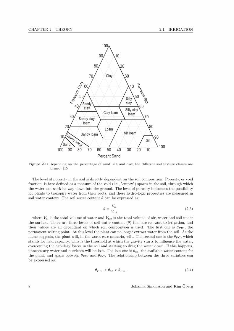
Figure 2.1: Depending on the percentage of sand, silt and clay, the different soil texture classes areformed. [15]
The level of porosity in the soil is directly dependent on the soil composition. Porosity, or voidfraction, is here defined as a measure of the void (i.e., "empty") spaces in the soil, through whichthe water can work its way down into the ground. The level of porosity influences the possibilityfor plants to transpire water from their roots, and these hydro-logic properties are measured insoil water content. The soil water content θ can be expressed as:
θ = VwVtot
(2.3)
where Vw is the total volume of water and Vtot is the total volume of air, water and soil underthe surface. There are three levels of soil water content (θ) that are relevant to irrigation, andtheir values are all dependant on which soil composition is used. The first one is θPW , thepermanent wilting point. At this level the plant can no longer extract water from the soil. As thename suggests, the plant will, in the worst case scenario, wilt. The second one is the θFC , whichstands for field capacity. This is the threshold at which the gravity starts to influence the water,overcoming the capillary forces in the soil and starting to drag the water down. If this happens,unnecessary water and nutrients will be lost. The last one is θac, the available water content forthe plant, and spans between θPW and θFC . The relationship between the three variables canbe expressed as:
θPW < θac < θFC . (2.4)
8 Johanna Simonsson and Kim Öberg
CHAPTER 2. THEORY 2.1. IRRIGATION
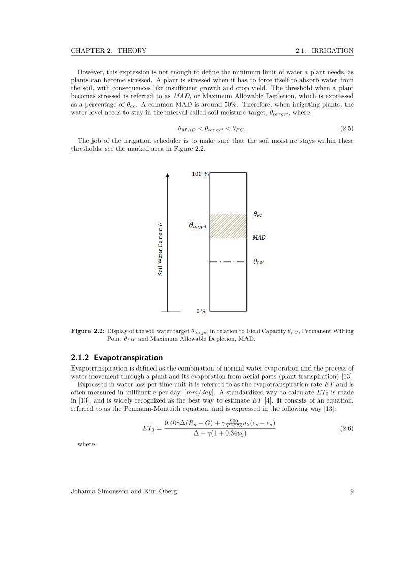
However, this expression is not enough to define the minimum limit of water a plant needs, asplants can become stressed. A plant is stressed when it has to force itself to absorb water fromthe soil, with consequences like insufficient growth and crop yield. The threshold when a plantbecomes stressed is referred to as MAD, or Maximum Allowable Depletion, which is expressedas a percentage of θac. A common MAD is around 50%. Therefore, when irrigating plants, thewater level needs to stay in the interval called soil moisture target, θtarget, where
θMAD < θtarget < θFC . (2.5)
The job of the irrigation scheduler is to make sure that the soil moisture stays within thesethresholds, see the marked area in Figure 2.2.
Figure 2.2: Display of the soil water target θtarget in relation to Field Capacity θF C , Permanent WiltingPoint θP W and Maximum Allowable Depletion, MAD.
2.1.2 EvapotranspirationEvapotranspiration is defined as the combination of normal water evaporation and the process ofwater movement through a plant and its evaporation from aerial parts (plant transpiration) [13].Expressed in water loss per time unit it is referred to as the evapotranspiration rate ET and is
often measured in millimetre per day, [mm/day]. A standardized way to calculate ET0 is madein [13], and is widely recognized as the best way to estimate ET [4]. It consists of an equation,referred to as the Penmann-Monteith equation, and is expressed in the following way [13]:
ET0 =0.408∆(Rn −G) + γ 900
T+273u2(es − ea)∆ + γ(1 + 0.34u2) (2.6)
where
Johanna Simonsson and Kim Öberg 9

CHAPTER 2. THEORY 2.1. IRRIGATION
ET0: reference evapotranspiration rate [mm/day]Rn: net radiation at the crop surface [MJ/m2/day]G: soil heat flux density [MJm−2day−1]T : mean daily air temperature at 2 m height ◦Ces − ea: saturation vapour pressure deficit [kPa]∆: slope vapout pressure curve [kPa◦C−1]γ: psychometric constant [kPa◦C−1]
Further analysis on how to calculate each of the variables can be found in [13].However, irrigation requirements differ between crops, soil and location and the same is true
for the evapotranspiration rate. To obtain an ET value for a specific crop, one must modify ET0.ET0 is the empirically derived constant evapotranspiration rate for grass. By multiplying it witha constant KC , as seen in equation
ETC = KC ·ET0, (2.7)
one can obtain the correct value for a certain crop. Kc is directly dependent on what type ofcrop is being grown, and what growth stage the crop resides in. Details about Kc and differentvalues can be found in [13, chap. 6].In order to further discuss and elaborate on the calculation of ET0 a proposed simplification
of Equation (2.6) will be used. Hargreaves and Samani [15] proposed the following equation forcalculating ET0:
ET0 = 0.0023 RA (T + 17.8)√TR (2.8)
where RA is extraterrestrial solar radiation, T is the mean air temperature in ◦C and TR isthe average daily temperature range for the considered time period. Since TR is influenced bysolar radiation, local advective energy and abrupt weather changes (storms), the equation willnot be accurate on days with large weather changes but it has been proven to deliver satisfactoryresults when T and TR are averaged over periods of five or more days [15].The extraterrestrial solar radiation is computed with the following equation:
RA = 37.6 dr(ωs sin φ sin δ + cos φ cos δ sinωs) (2.9)
where RA is in units of MJ/m2/day, dr is the relative distance from the earth to the sun, ωsis the sunset hour angle (rad), φ is the latitude (rad) and δ the declination of the sun (rad) [15]and they are defined as:
δ = 0.4093sin 2π(284 + J)365 (2.10)
dr = 1 + 0.033 cos(
2πJ365
)(2.11)
ωs = cos−1(−tanφ tan δ) (2.12)
where J is the calendar day (1-365).Once the value of ET0 has been calculated the choice of Kc can be made. Kc is directly de-
pendent on what type of crop that is grown, and what growth stage the crop resides in. Detailsabout Kc and different values can be found in [13, chap. 6].
10 Johanna Simonsson and Kim Öberg

CHAPTER 2. THEORY 2.1. IRRIGATION
Example calculation of RA:For 27◦N latitude (φ = 0.4712 rad) on January 8th, the value of δ is -0.3893, dr is 1.0327 andωs is 1.3602. From Equation (2.9) the value of RA is 22.20 MJ/m2/day.
Figure 2.3: Curves of RA in MJ/m2/day for northern latitudes 0◦ to 55◦ with 4◦ increments. [15]
As can be seen in Figure 2.3 there is a relatively high annual variation in extraterrestrial solarradiation at the higher latitudes, whereas the variation at the equator is minimal. This leads tothe conclusion that year-round cropping is a possibility at low latitudes, particularly within thetropics (23.5◦N and ◦S) [15].
Johanna Simonsson and Kim Öberg 11

CHAPTER 2. THEORY 2.2. CHARACTERISTICS OF WIRELESS SENSOR NETWORKS
2.2 Characteristics of wireless sensor networksWhen constructing an autonomous irrigation system, power management will inevitably play apart of any successful installation. One of the most influential parameters on power consumptionin WSNs is the routing scheme, as a poorly chosen one will cause the nodes’ radio to idle listenwhen not necessary and perhaps forward packages along sub-optimal routes to the sink, causingunnecessary battery depletion in the process.This section will outline the major design decisions that have to be made when designing
an autonomous irrigation system based on WSN technology. It will also highlight the differentparameters for which optimization can be made.
2.2.1 System dynamicsWhen constructing a wireless sensor network with the subsequent topology choices and routingschemes it is important to first conclude which type of system it will be applied on. Systems areoften categorized into proactive and reactive. Proactive systems are defined by long sleep periodsand pre-scheduled intermittent wake-ups, upon which all nodes either collect sensor data and/orforward data to the base station. This kind of system is very well suited for implementations suchas habitat monitoring, intelligent buildings and precision agriculture, to mention a few. [16, 17]Contrary to proactive systems, reactive systems sleep less and are pinged for sensor data upon
user’s request or if there’s a critical change in the network field. Such a network is aptly builtfor battlefield and machine surveillance, earth movement detection, wild animal monitoring andindustrial applications, among others. [17]However, not all implementations of a wireless sensor network are strictly proactive or reac-
tive, combination systems exist and are referred to as hybrid systems. For a complete set ofdistinguishing characteristics of the two systems see Table I.
Table I: Characteristics of proactive and reactive networks [16].Description Proactive ReactiveApplication type Periodic monitoring Critical monitoring/Event detectionMode of sensing circuitry Periodically switch on Always onMode of communication device Periodic switch on Always onData delivery Periodic/continous Event driven/On demand
Seeing as this thesis concerns a system which is to be deployed in an agricultural context, itcan be concluded that the system should be categorized as proactive. The aim is for the nodes toonly wake up and/or do sensor readings when absolutely necessary and go into idle or sleep modein between those events. Furthermore, monitoring of crops is a slow process even when talkingabout "rapid" weather changes (an approaching cold front can take up to 6 hours to arrive [5])and therefore no reactive system characteristics are needed.
2.2.2 Deployment of nodesAnother important factor, when deciding on a routing protocol, is whether the nodes will berandomly or deterministically deployed. Deployed in this context refers to how to nodes arephysically placed in the monitored area. Deterministic deployment has many advantages, suchas: even node distribution within the network area, less interference and less unnecessary overlapin coverage.However, deterministic deployment is only possible when the area is easily accessible, for hostile
and unreachable areas random deployment is the only option. As a result, a larger quantity of
12 Johanna Simonsson and Kim Öberg

CHAPTER 2. THEORY 2.2. CHARACTERISTICS OF WIRELESS SENSOR NETWORKS
nodes are required to make sure that, despite the uneven distribution, the entire area of interestis covered. This however, in turn, leads to a higher probability of two nodes overlapping, andthereby registering the same data, often referred to as data redundancy, see Figure 2.4. [16]
Figure 2.4: The data redundancy issue. Node A and B overlap and will both be reporting sensor dataregarding area r to the sink node C. [18]
In the field of agriculture and irrigation, it is most likely that deterministic deployment will beused seeing as the monitored area by definition is reachable since it’s being used for agriculturalpurposes and thereby must be possible to harvest.
2.2.3 Network topologyEven though the underlying deployment of nodes might be deterministic the choice of networktopology can still vary greatly. The term network topology here refers to how nodes are deployed,related and connected to each other within the network. The flow of data will therefore besignificantly different depending on which topology is chosen (the term includes both hard-wirednetworks as well as wireless).There are currently eight different known topologies, and those best suited for wireless im-
plementation are mesh, tree and star network [19, p. 121]. These three will be the topologiesstudied for the chosen implementation. A good network topology should be able to transfer databack and forth between nodes or to a main computer, and, if scalability is a goal, be able toimplement an infinite number of nodes on an infinitely large area.
Mesh topology
The principle of a wireless mesh network is that a node can communicate (transmit data) to anyone of its one-hop neighbours, see Figure 2.5. When a message is transmitted from one of thenodes, the other nodes act as routers by forwarding the message to its destination. The goal isoften to achieve the shortest route or minimize the number of hops, which can be accomplishedby smart algorithms based on the knowledge of the network. This ensures that the hops betweenthe nodes are as few as possible, saving energy and increasing the speed. A central server forcomputation may or may not be implemented, depending on the implementation. [20]
Johanna Simonsson and Kim Öberg 13
CHAPTER 2. THEORY 2.2. CHARACTERISTICS OF WIRELESS SENSOR NETWORKS
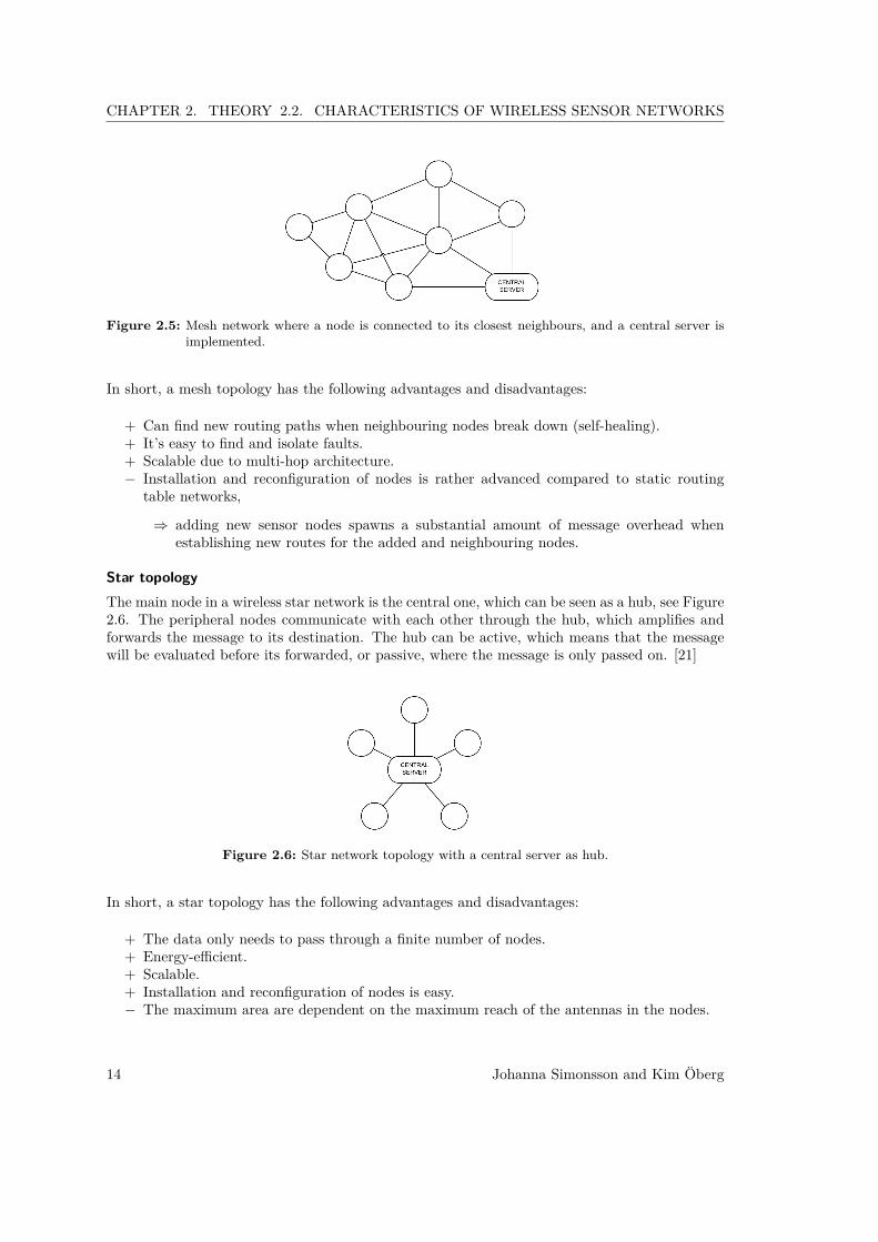
Figure 2.5: Mesh network where a node is connected to its closest neighbours, and a central server isimplemented.
In short, a mesh topology has the following advantages and disadvantages:
+ Can find new routing paths when neighbouring nodes break down (self-healing).+ It’s easy to find and isolate faults.+ Scalable due to multi-hop architecture.− Installation and reconfiguration of nodes is rather advanced compared to static routing
table networks,
⇒ adding new sensor nodes spawns a substantial amount of message overhead whenestablishing new routes for the added and neighbouring nodes.
Star topologyThe main node in a wireless star network is the central one, which can be seen as a hub, see Figure2.6. The peripheral nodes communicate with each other through the hub, which amplifies andforwards the message to its destination. The hub can be active, which means that the messagewill be evaluated before its forwarded, or passive, where the message is only passed on. [21]
Figure 2.6: Star network topology with a central server as hub.
In short, a star topology has the following advantages and disadvantages:
+ The data only needs to pass through a finite number of nodes.+ Energy-efficient.+ Scalable.+ Installation and reconfiguration of nodes is easy.− The maximum area are dependent on the maximum reach of the antennas in the nodes.
14 Johanna Simonsson and Kim Öberg

CHAPTER 2. THEORY 2.2. CHARACTERISTICS OF WIRELESS SENSOR NETWORKS
Tree topologyThe tree structure is a hierarchical topology which begins with a root node. From this root nodethe tree branches out to leaves, the number dependent on the branching factor f , see Figure 2.7.If f = 1, the topology is linear, where as if f = n, each node can have up to n leaves branchingout. The nodes communicate with each other through point-to-point links. The central server,which evaluates the data, is the root node. The main branches from the root is called backbone,and is where most of the information will travel. [22]
Figure 2.7: Network topology of a tree structure with branching factor f = 2.
In short, a tree topology has the following advantages and disadvantages:
+ Flow of data is easy to follow.+ Scalable.− Dependant on backbone branch.− Connection between nodes needs to be predefined.
2.2.4 RoutingOn top of these topologies a routing scheme is chosen. Which routing protocol the networkemploys is tightly linked to the chosen network topology but not inherently dependent thereof.Network topology will therefore be abstracted away from the following section in order to focuson the specific algorithms for routing.Sensor nodes are constrained in bandwidth, often deployed over large, sometimes hard to reach,
areas and required to operate, for long periods of time, disconnected from the power grid [18].These characteristics translate to a number of challenges in the area of energy consumptionoptimization. In the network layer, of the network protocol stack, the main aim is therefore toconstruct energy efficient routing and reliable relaying of data without compromising the networklifetime.The main duties of the network layer is to enable routing and forwarding, others include
creating and maintaining a network topology. The two main questions a routing protocol mustanswer are the following:
• How to provide information for wise forwarding decisions?• How to organize the forwarding?
A close to optimal solution to these questions would be to utilize a proactive protocol designedto always find the shortest path from sender to destination while simultaneously minimizing the
Johanna Simonsson and Kim Öberg 15

CHAPTER 2. THEORY 2.2. CHARACTERISTICS OF WIRELESS SENSOR NETWORKS
number of hops and the energy consumed. However, such a protocol would require each node tostore and keep track of all links in the network, a virtual impossibility when dealing with memoryconstrained WSN nodes.In other words, routing in WSNs is a challenge in comparison to ordinary communication and
wireless ad-hoc networks because of the following inherent characteristics:
• The flow of data from different areas is directed towards a particular sink node, possiblyresulting in traffic congestion, packet collision and bottle necks.
• The sensor data traffic suffers from redundancy issues as several nodes often register thesame phenomenon.
• Sensor nodes are constrained in terms of transmission power, energy supplies, processingand memory capacity.
These characteristics have resulted in a number of WSN specific algorithms for routing, whichcan be categorized into data-centric (flat), hierarchical and location-based protocols [18]. Hi-erarchical protocols have many advantages, such as better scalability, higher efficiency of datagathering and better capability of load balancing than flat protocols [23]. However, flat protocolsare still commonly used and are the base of the hierarchical ones, therefore protocols from bothcategories will be presented in this section. Location based protocols will not be covered as theyare configured with mobile ad hoc networks in mind and therefore not optimized for a staticdeterministic node deployment within agriculture [24].
2.2.5 Data-centric protocolsSome of the most common and earliest routing protocols for WSNs are the data centric (flat)protocols, among which direct-transmit, flooding and gossiping are the three basic choices [16].
Direct transmissionIn small, non-scalable networks, the easiest and most straight forward approach to routing isdirect transmission, which means that each node directly transmits its data to the base station,see Figure 2.8.
Figure 2.8: Model of direct transmission [16].
To understand the weakness of such a protocol, consider the fact that the farther away nodesare placed from the base station, the more energy (stronger radio signals) will be consumed when
16 Johanna Simonsson and Kim Öberg

CHAPTER 2. THEORY 2.2. CHARACTERISTICS OF WIRELESS SENSOR NETWORKS
transmitting a message. Furthermore, packets travelling long distances will also encounter moreobstacles and the risk for packet loss is thereby greater.When considering this it becomes clear that the nodes farthest away from the base station will
die out much quicker, leaving that area of the network unmonitored. Thus, direct transmissionis only suitable for the nodes closest to the base station or for very small, non-scalable networks.As a solution to the issues introduced by direct transmission, short distance travel protocols,
such as flooding and gossiping, have been developed. In these multi-hop architectures (see Figure2.9) all nodes work together by passing on the data to its closest neighbour, thereby reducing theaverage energy consumed by the far away nodes and thus the overall power consumption of thenetwork. [16]
Figure 2.9: Model of multi-hop transmission [16].
FloodingFlooding works in a broadcasting manner, which means that each node broadcast its data to allneighbouring nodes which then forward the data in the same manner until it reaches the sinknode. With this approach no routing tables are needed since all nodes take part in the handlingof each data packet. This leads to very low transmission delays but also unnecessary energy usagewhen all nodes handle every packet transmission in the network. [16]Another issue introduced by flooding is data implosion, meaning one node receives multiple
copies of the same data, see Figure 2.10.
Figure 2.10: Implosion issues in the flooding protocol [16].
As seen in Figure 2.10 above, node 4 will receive multiple copies of the same sensed datasince node 1 will forward its data to node 2, 3 and 4 and node 2 and 3 will in turn forward the
Johanna Simonsson and Kim Öberg 17

CHAPTER 2. THEORY 2.2. CHARACTERISTICS OF WIRELESS SENSOR NETWORKS
same data to node 4, 5 and 6. The data is forwarded in the same manner throughout the entirenetwork until it reaches the sink which causes multiple unnecessary transmissions, and therebyenergy losses.
GossipingGossiping solves the implosion problem by randomly selecting a neighbour to pass the data to,instead of broadcasting to all nearby nodes. However, this introduces uncertainty as to whetherthe data packet will actually reach the base station and even if it does, it’s very likely to haveaccumulated quite serious transmission delays along the way. [16]
2.2.6 Hierarchical routing protocolsThe point of deploying a hierarchical routing protocol is to ensure that some nodes take respon-sibility to perform high energy transmissions while the rest perform normal tasks. This becomesparticularly important in large scale networks where direct transmission or other flat protocolswould dissipate too much energy.Within the category of hierarchical routing protocols there are two sub-categories: cluster-
based and chain-based. In cluster based routing, the nodes are organized in clusters with acluster head. The cluster head reduces the energy consumption of the cluster by receiving clusternode data and aggregating it before forwarding it to the sink node.Load balancing is done through a multi-path scheme for data transmission from the cluster
head to the base station, meaning data can travel along several different paths on its way to thebase station. [23]The key in chain-based routing however is to form chains among the nodes so that each node will
receive and transmit only to one pre-determined one hop-neighbour. Data is thereby aggregatedthrough the chain until it reaches the chain leader which transmits directly to the base station.This way of keeping transmission signals weak (since they only travel short distances) and utilizingdata aggregation reduces the average energy spent by each node in the chain. However, since eachnode in the chain only has one parent node, node failure inevitably leads to packet loss. Addingnodes is also a high energy task as either the whole chain needs to be reconstructed (spawning alarge amount of control overhead) or the new node might have to join the chain in a sub-optimalway. Sub-optimal refers to the situation when a node is added to an area in which all other nodesalready are a part of the chain (a node can only exist in one unique place in the chain at once)meaning the node will have to connect to another node much farther away, causing long distancehigh-energy transmissions. [25]For this reason, the cluster based schemes will be the focus of this section and particularly
LEACH which is a popular and well establish protocol [26].
LEACHLEACH, Low-Energy Adaptive Clustering Hierarchy, is a cluster-based hierarchical routing pro-tocol which employs adaptive cluster head rotation. This means that instead of forming clusterswith static cluster heads, the role of being the cluster head is rotated among the nodes eachround of transmission. Each round consists of two phases, the set-up phase and the steady-statephase.In the set-up phase, each node randomly selects a number between 0 and 1, and elects itself
cluster head if that number is less than the threshold value T (n) which is computed with thefollowing equation:
T (n) = p
1− p(r·mod 1p ), (2.13)
18 Johanna Simonsson and Kim Öberg

CHAPTER 2. THEORY 2.2. CHARACTERISTICS OF WIRELESS SENSOR NETWORKS
where p is the optimal number of cluster heads (estimated at 5% of the total number of nodes),r is the current transmission round and n ∈ G, where G is the set of nodes which have not beencluster heads in the last 1
p rounds. [18]
The self-elected cluster heads will then advertise their status to the neighbouring nodes bybroadcasting an advertisement message (ADV). The neighbouring nodes will then choose to jointhe closest cluster head in order to minimize the transmission distance. The choice of whichcluster head is the closest is based on which advertisement message is the strongest (all messagesare sent at the same transmit energy).
Figure 2.11: Implosion issues in the flooding protocol [16].
When all clusters have formed the steady-state phase begins, in which data from all nodes areforwarded to the base station. After this a new round begins with new clusters and cluster heads.To balance the load among the nodes, a cluster head node is not eligible to become cluster headagain within the next 1
p rounds. This approach significantly postpones the occurrence of first nodedies (FND), thereby prolonging the lifetime of the network. Compared to direct transmissionand minimum transmission energy (multi-hop), LEACH is about two times better than the firstand four times better than the latter, see Figure 2.11.
However, some issues are introduced by LEACH as well. In the steady-state phase each nodein the cluster is awarded a guaranteed time-slot by the cluster head, in which data from the nodeshould be forwarded to the cluster head. This works fine for reasonably sized clusters but sincecluster formation in LEACH is fully distributed and requires no global knowledge of the network,clusters are not uniformly sized [18]. This leads to packet losses in oversized clusters since thesteady-state duration of one transmission round is fixed for the whole network, meaning all nodesin the oversized cluster will not be guaranteed a time slot each round, see Figure 2.12.
Johanna Simonsson and Kim Öberg 19

CHAPTER 2. THEORY 2.2. CHARACTERISTICS OF WIRELESS SENSOR NETWORKS
Figure 2.12: Time line for a small (a) and large (b) LEACH-cluster [16].
Therefore, LEACH is only suitable for low data traffic applications. Furthermore, since LEACHutilizes single-hop routing where each node can transmit directly to the cluster head or basestation it also falls short in applications where the sensor nodes are deployed in large regions.
2.2.7 Power consumptionDue to the power consumption constraint in most WSNs, it is important to evaluate exactly whatconsumes power in the system. This section will review what consumes power in a sensor node,and how to minimize the consumption for the MCU.When minimizing power consumption for nodes in a WSN, the aim is to prolong the life span
of each node as much as possible. The life span tlife of a node is decided by the battery energycapacity, Ebattery, according to the following relationship:
Ebattery =∫ tlife
0Pnode(t) dt, (2.14)
where Pnode(t) is the power which variates over the time t. The power Pnode is the sum of thepower drawn by all the components in the node, and is denoted by:
Pnode =n∑i=1
Pi . (2.15)
where n is the total number of components. Components that consume power in a sensor nodelike [27, 28, 29] include:
• PMCU : Microcontroller• Pflash : Flash Memory• Pradio : Radio Transceiver• Psensor : Sensors• PLED : LEDs
If the system is defined as a proactive one, like most applications in precision agriculture, thenode will sleep for long intervals, wake up to sample data and then send/forward to the basestation, see Section 2.2.1. The normal procedure for a sensor node will then be:
20 Johanna Simonsson and Kim Öberg

CHAPTER 2. THEORY 2.2. CHARACTERISTICS OF WIRELESS SENSOR NETWORKS
1. Wake up from sleep state.2. Turn on sensor.3. Do sensor measurements.4. Turn off sensor.5. Turn on radio.6. Wait for acknowledgement to send.7. Send data via the radio.8. Turn off the radio.9. Go back to sleep.
If the power of the node is averaged out every active sampling cycle, Pactive,avg, the previouslymentioned procedure can be summarized as:
Ecycle = Pactive,avg ·Tactive, (2.16)
Figure 2.13: Power consumption for a sampling cycle for one sensor node.
see Figure 2.13, where T is the period of the system. As commonly known, the power P inelectrical circuits is defined as:
P = U · I, (2.17)
and as the required voltage level is predefined by the sensor circuit, the goal is to minimize thecurrent consumption of each component i, and the time ti that each component is active.
Johanna Simonsson and Kim Öberg 21


3 State of the ArtUnlike the theory chapter this part of the thesis aims to cover what is at the forefront of thedifferent areas of the regarding system design within the agricultural domain aimed at irrigation.
3.1 Smart autonomous irrigationSmart autonomous irrigation is a fast-growing development area due to the advancements inother scientific fields, like sensor technology and internet availability. A lot of the advancementshave been made in the United States of America, where also most of the companies and productsreviewed in this section have emerged.An autonomous irrigation system is defined as a system that irrigates without the user inter-
fering. The ’dumb’ autonomous system is referred to as a irrigation clock. It works as the namesuggests, irrigating after a periodically set timer, and is the standard system used in the industry.However, this puts demands on the user to make sure the system does not over- or under irrigatethe crops. In comparison, a smart irrigation system is defined as a system in which the waterdistribution, both in timing and amount, is changed dynamically with respect to outer factors.[4]
Terms and conceptsTo understand the concept of irrigation and the products on the market today, a few terms andconcepts have to be explained:
• A ’smart’ irrigation unit is referred to as a controller.• To convert an existing ’dumb’ irrigation unit (ex. an irrigation clock) into a controller, the
user can approach the problem in two ways. The controller can either be integrated with thealready existing system (Add-On) or it can replace the old system entirely (Stand-Alone).
• All products mentioned in this section are run on 24 VAC, converted from 110-120 VAC.• All the controllers utilize a MCU to calculate and schedule irrigation.• Most modern irrigation systems can schedule the watering amount and timing differently
in different zones. A zone is the area watered by one or more water distributors, like oneor more sprinklers. Different zones may have different properties, like plant type or slopeangle, and programming the water distribution differently for each zone may be crucial forefficient irrigation. [4]
There are a few ways to implement said smart system, and two dominating techniques for smartautonomous irrigation on the market today is the weather-based approach and the soil moisturesensor approach. A few products enhances the performance in the weather based calculation byutilizing a soil moisture sensor, and those are mentioned in the end of this section. The differentapproaches are presented in Section 3.1.1 to 3.1.2.
3.1.1 Irrigation based on weatherBy monitoring the weather conditions of the area, a weather-based system can utilize the ET -Equation (2.6) in conjunction with the Soil water balance Equation (2.2) to estimate the neededirrigation.
23

CHAPTER 3. STATE OF THE ART 3.1. SMART AUTONOMOUS IRRIGATION
Simply put, the controllers estimate how much water is depleted from the soil and then com-pensate the water loss with irrigation. The goal is to keep the plants within the thresholds oftheir soil moisture target, see Section 2.1.1. The more accurate the calculations of ET are, thebetter the applied amount of water mirrors the plants’ need. The accuracy of the ET equations isimproved by monitoring as much of the variables locally, and not relying on standard or remotelycalculated values. To adjust the system to every location’s unique characteristics, variables likesoil properties, plant type, root depth, slope conditions etc. are often defined in the system toget more accurate irrigation calculations. The available monitoring techniques will be presentedin the rest of Section 3.1.1.
Historical ET schedulingAs ET often has the same value for the same time every year, scheduling irrigation with historicalET determined by time of year and zip code (location of the field of interest) is therefore possible.The historical data is stored in the MCU memory. This is implemented as the main source of datain [30] product, and used as a complement together with weather sensors in products [31] and[32]. It can also be a back-up solution when the main source of information fails to be acquired,as is done by the controllers [31] and [33]. The irrigation for this solution changes dynamically,but as the data is predefined the system is not ’smart’ in the defined sense mentioned in thebeginning of the section.
Weather sensorsAs weather is an unpredictable force of nature, there are a lot of different parameters that canbe measured to anticipate what the weather will be like. A few of these parameters are relevantto the ET -equation, and can be monitored with different sensors. The sensors mostly utilizedare different kinds of rain sensors. Most of the systems on the market, like those reviewed in [4],include a rain sensor or rain gauge, or include the possibility to add one to the existing system[4, p. 11] [34].A well-implemented feature among those who have integrated rain sensors, is that whenever
rain starts falling, the current irrigation scheduling is interrupted. The irrigation is then put onhold until the rain stops, as implemented in the controller [35]. This is done to prevent water frombeing wasted. Some systems, like [36], have integrated air temperature sensors that can shut downirrigation if the temperature drops below 0 ◦C, to keep the plants from freezing. Other weathersensors worth mentioning are wind, solar and relative humidity sensors, which help increase theaccuracy of the ET equation. Such sensors are used in [37], [36] and [38]. Some systems, like [39]and [40], actually utilize or can integrate a fully functioning local weather station.
Weather station dataIrrigation can, apart from using historical ET -data and locally implementing sensors, be sched-uled with data acquired from online weather services, as done by the products [41] and [42]. Ifthis kind of service is implemented, the data can be collected from 9,000 [39] up to 44,000 weatherstations [42]. Due to many commercial and residential implementations of autonomous irrigationsystems that upload their locally calculated ET to the Internet, websites monitoring this ET isnow available for private and commercial use [43]. This means that more systems can utilize thisdata, speeding up the implementation of autonomous systems even more.The same interrupt feature used by rain sensors, to turn off the scheduled irrigation when rain
starts falling, is used by weather station data systems, like done in [44].The use of a locally implemented weather station versus the use of collecting data from online
weather forecast services can be discussed. As previously established, the more data that isacquired locally, the more accurate the ET equation will become. With that said, if more sensors
24 Johanna Simonsson and Kim Öberg
CHAPTER 3. STATE OF THE ART 3.2. WSN IN PRECISION AGRICULTURE
are implemented, the accuracy will increase. However, if the price is an issue, it is of coursebetter to rely on data from other weather stations. If the system should choose what weathersensor to integrate, the rain sensor is the most popular one, and also the most useful due to therain interrupting feature and in use to prevent over-irrigation [4].If the irrigation system collects data from a weather station, the controller needs to have access
to internet. Products that have implemented this feature take advantage of the internet accessby creating a two-way communication. This means that the user can monitor the system fromafar, by using interfaces like a computer or smart phone, as done by [44]. Other features, asimplemented by [45] and [39], includes changing the irrigation schedule and update plant types.A few systems, like [37], that does not utilize weather station data have internet access as anadd-on feature, as well as radio remote controls.
3.1.2 Irrigation based on sensorsMost of the smart irrigation systems that utilize soil moisture sensors work in the same way. Thecontroller is attached as an Add-On onto the existing timer-based irrigation scheduler, and usesinterrupts to change the default timer settings. The sensor is wired to the control box, where asoil moisture target threshold, known as a ’trigger point’, has been programmed. This triggerpoint value can be set by the user, or calculated by the system ([46]) if it is a more sophisticatedone. If the soil moisture is less than the pre-programmed threshold value, the controller urgesthe system to irrigate right away. This is known as a reactive system and can be seen as analarm-mechanism, preventing the soil from ever getting too dry. At all other times, the standardtimer will conduct the irrigation, as products [47], [37] and [48] have done. As the sensors arewired, often along the same wires that control the valves, it is impractical to use more than afew sensors [49]. This means one soil moisture sensor is used to control more than one zone, eventhough the zones have different water needs and ET -constant. This can be a more or less seriousissue depending on the plants being grown.The product supplied by [40] can integrate their soil moisture sensor with the ET -calculations
supplied by weather data, to create a feedback system. This addresses the issue with not knowingthe initial moisture levels when irrigating, and during the process validates the accuracy of theET values.
3.2 WSN in precision agricultureAll of the mentioned available solutions above have one thing in common, assumptions of het-erogeneity as none of them provide the dense monitoring needed in order to adapt the irrigationto the micro-climate fluctuations within the area. Dense monitoring here refers to the possi-bility, provided by wireless sensors, to monitor crop close enough to register fluctuations in themicro-climate, the term together with used metrics are further explained in Section 6.1.1.However, contrary to these existing approaches, precision agriculture aims at eradicating these
assumptions of heterogeneity. Precision agriculture in this context refers to the four-stage processusing techniques to observe spatial variability [50]:
• Geolocation: The land being cultivated is delineated in order to be able to overlay infor-mation gathered from soil analysis and information on previous crops and soil resistivity.
• Characterizing variability: Fluctuations and variations in the field can depend on anumber of factors, such as climatic conditions (hail, drought, rain, etc.), soils (texture,depth, nitrogen levels), weeds and disease. These are monitored either by permanent indi-cators (soil indicators), which provide information on the environmental constants, or bypoint indicators (weather station, temperature/light sensors, soil moisture sensors), which
Johanna Simonsson and Kim Öberg 25

CHAPTER 3. STATE OF THE ART 3.2. WSN IN PRECISION AGRICULTURE
allows tracking of a crop’s status, i.e. possible disease outbreaks, water stress, nitrogenstress, frost damage and so on. Permanent indicators combined with point indicators makeit possible to precisely map agro-pedological conditions.
• Decision-making: How to act on the gathered data.– Predictive approach: Decisions are based on analysis of static (permanent) indicators
during the crop cycle.– Control approach: Decisions are based on analysis of static (permanent) indicators
which are updated during the crop cycle by sampling, remote sensing or satellitesensing (for example).
• Adapt practices: Adjust irrigation, harvest schedule and seed density during seed timeaccording to the geological variations of the crop.
It is in the context of precision agriculture that WSNs becomes interesting. As mentioned inSection 1.1 WSNs have just recently been gaining momentum in the field of agriculture. Between2004 and 2010 several interesting studies, such as [7, 5, 6, 9], were carried out with the aim ofestablishing whether the dense monitoring provided by the WSN technology would prove to beagricultural significant. In other words, how much of an issue are the now used assumptions ofheterogeneity and are there other, yet unknown, advantages of such dense monitoring?The answer turned out to be yes as the research conducted proved that the monitored fluc-
tuations of the micro-climate (provided by the dense monitoring) indeed is of importance whentracking everything from irrigation needs and fruit maturity to heat accumulation and possiblepest outbreaks [7, 5, 6].Although almost all existing irrigation systems today still neglect this fact, there are in fact
a few crop-monitoring solutions on the market today that monitor the micro-climate. Thisimplementation is referred to as Wireless Crop Monitoring.
3.2.1 Wireless crop monitoringApart from the smart irrigation systems, there are a few wireless crop monitoring systems on themarket. They utilize wireless communication and multiple sensors to monitor all kinds of relevantenvironmental data. The data is not used to correct irrigation, but to analyse the micro-climateto enable the user to do improvements as deemed necessary. The implementations have somecommon traits worth mentioning:
• Energy Source: The wireless units on the market are all, as the name suggest, discon-nected from the power grid. [51] utilizes both 3 AA batteries and solar panels as energysources, while [52] uses 2 AA alkaline batteries.
• Communication Protocol: [51] uses a low-power mesh network over a 802.15.4 protocolto communicate, while [52] and [53] uses direct transmission. [53] have repeaters that canbe implemented that strengthens the signal from the field unit to the base station.
• Expected life span: [53] have a life expectancy of up to 6 years on the built in long-lifeinternal battery source, while [52] have 6 months. Without the solar panels [51] have a lifeexpectancy of 3 months, but if the panels are utilized the unit is estimated to survive morethan 5 years.
• Reach: The product [52] have a reach up to 300 m, whereas [53] and [51] have a range upto 3 km.
26 Johanna Simonsson and Kim Öberg

CHAPTER 3. STATE OF THE ART 3.3. SYSTEM DESIGN
• Sampling Interval: The sampling interval ranges (as default values) from 1 [52] to 15 [51]minutes.
The usage of the mentioned units differs. The [52] wireless sensing units are paired with amonitoring unit that can interact with up to 16 sensing units. 8 of these units can be set totrigger an alarm. [51] uses a ”Base Radio” to be connected to a Gateway device run on DebianLinux, to provide an interface to view data, run reports and set up alarms if any of the collecteddata is out of the ordinary. [53] uses a base station receiver that is to be plugged into a PC.Software provided by [53] is intended to help the user to analyse the crops and schedule theirrigation better, but not as a first-hand controller. These three systems are not intended to beutilized directly with a smart irrigation scheduler, but more as a tool to analyse the crops andthen manually correct the irrigation if needed.All the products can utilize sensors that monitor the environment. [51] have 4 sensor ports
where the 4 sensors provided by the manufacturer can be integrated. [52] utilizes air temperatureand relative humidity sensors. [53] can integrate everything from soil moisture, pressure, air andsoil temperature sensors to be used together with a fully working weather station.This leads to the conclusion that there exists WSN solutions for precision agriculture, but they
are not well integrated with the actual irrigation.
3.3 System designAs proven in Section 3.1, detailing the market for irrigation systems and wireless crop monitoring,the different design aims vary greatly from product to product and very few have made the energyefficiency of the system a priority. Certain systems even utilise wired sensors like [49, 47, 37],and others AA batteries with varying lifetime [51, 52].The reason WSN versions of irrigation systems haven’t made power consumption a priority
(yet) is largely due to the fact that WSNs just recently started gaining momentum in the fieldof agriculture and that together with cheaper hardware and emerging non-proprietary softwarechanged the conditions.As a result, very few out of the conducted studies ([7, 5, 6, 9, 54, 55]) (performed between
2004-2010) put much, if any, effort into the power management aspect of the network design.Furthermore, it’s not just a matter of power optimization, there’s a permanent trade-off be-tween power management and robustness that for every given WSN implementation needs to beaddressed.This section will therefore present the existing approaches and solutions to the power manage-
ment and robustness design choices.
3.3.1 DeploymentAs mentioned in the Theory chapter, node deployment can either be random or deterministic.Since farm lands are inherently easily accessible (because they are harvested), and not seldom alsoquite uniform in size and dimension, deterministic deployment is most frequently used. Randomdeployment serves no purpose in an agricultural context where coverage is the main goal anddata redundancy something to be avoided. This is evident since all the studies in [7, 5, 6, 9, 55]have utilized deterministic deployment of nodes.In [7] the aim was to position the nodes in a very dense grid pattern in order to investigate
how dense the monitoring needed to be for the data to be agricultural significant. They reachedthe conclusion that depending on what parameters are being monitored the density of the net-work may vary. For temperature profiles and fruit maturity for example, nodes 25 meters apartwould suffice, whereas nodes needed to be closer (15 m) to monitor possible pest outbreaks or
Johanna Simonsson and Kim Öberg 27

CHAPTER 3. STATE OF THE ART 3.3. SYSTEM DESIGN
frost damage. Thus, the prevailing node deployment has been and probably will continue to bedeterministic deployment because of the inherent characteristics of agriculture.The density of the monitoring however, remains tightly linked to the implementation and
isn’t an absolute number that can be applied in all settings. As is pointed out in [7, 5, 6, 9]the successful implementation of an autonomous WSN irrigation system postulates the helpof biologists, ethnographic research, farmers and agricultural specialists in order to design thesystem correctly.
3.3.2 Routing power consumptionWhen designing a robust and power smart irrigation network, routing is of utmost importance.This since the possibility of hardware power handling today is mostly already taken care of by theoperating system automatically (see Section 4.3 Node specifications in Method). What remainsthen is how to organize the network itself and the data forwarding.When comparing the performance of two or more routing protocols different approaches can
be useful. To get an indication of how well suited certain protocols are for an already knowntestbed, the First Order Radio model can be of great use [56]. It is an analytical model frequentlyused in WSN research to estimate the power consumption of a routing protocol and is usually thefirst step in the evaluation of a new protocol. The results are then often compared to simulationresults (COOJA/TOSSIM) and possibly even actual deployment data, with very good results.[1, 57, 58, 59]According to the hardware independent First Order Radio model the energy consumed by the
electronics needed to operate the transceiver circuit is Eelec = 50nJbit and the energy needed torun the transmitter amplifier is εamp = 100 pJbit/m2. This results in the following equations forreceiving and transmitting a k bit message over a distance d.
ETx(k, d) = Eelec · k + εamp · k· d2 (3.1)ERx(k) = Eelec · k (3.2)
As shown in the equations, both transmitting and receiving a message is a high overheadprocedure, which is why both should be kept to a minimum. However, it’s more complicatedthan that. In the Direct Transmission protocol receiving overhead is minimized since all nodestransmit to the sink, but at the same time the transmission costs are huge due to the largedistances packets have to travel. This means that for a flat protocol the worst case scenario ofhow far a node must transmit is inherently dependent on the scale of the system and the node’sdistance from the sink node. In other words such a protocol doesn’t scale well at all.In multi-hop protocols however (which minimize travel distance), transmission are kept very
short but then the number of receiving actions increase dramatically. In other words, a multi-hopprotocol might not necessarily improve the battery lifetime since an ill-suited algorithm couldcause data to travel via sub-optimal routes to the sink and thereby require too many relayingoperations.This leads to the conclusion that routing protocols must always be well tailored to their im-
plementations. However, with the help of Equation (3.1) and (3.2) the situation when directtransmission consumes the same amount as multi-hop can be found, see Section 3.3.2 below.
Direct Transmission vs Multi-hopConsider Equation (3.1) and (3.2), the difference between DT and multi-hop is that rather thanjust one (high-energy) transmit of the data (DT), each data message must go through n lowenergy transmits and n receives (multi-hop). [57] [60]:
28 Johanna Simonsson and Kim Öberg

CHAPTER 3. STATE OF THE ART 3.3. SYSTEM DESIGN
And depending on the cost for those operations the total energy expended in the system mightbe greater using multi-hop than direct transmission to the base station. This phenomenon isillustrated in Figure 3.1.
Figure 3.1: Four nodes, r distance apart.
As seen in Figure 3.1 the distance d can be rewritten as d = n· r, since all nodes in adeterministic deployment are stationary leading to the fact that the distance from sensor nodeto sink node is fixed. Thus, Equation (3.1) can be rewritten as:
ETx(k, d) = Eelec · k + εamp · k· d2 (3.3)= Eelec · k + εamp · k· (n· r)2 (3.4)= k(Eelec + εamp ·n2 · r2) (3.5)
In multi-hop routing, each node sends a message to the closest node on the way to the sinknode. Thus the node located a distance n· r from the sink node would require n transmits adistance r and n− 1 receives. This leads to:
Emulti−hop = n ETx(k, d = r) + (n− 1) ERx(k) (3.6)= n (Eelec · k + εamp · k· r2) + (n− 1) (Eelec · k) (3.7)= k ( (2n− 1)Eelec + εampnr
2 ) (3.8)
Thence, direct transmission requires less energy than multi-hop if:
Edirect < Emulti−hop (3.9)Eelec + εampn
2r2 < (2n− 1)Eelec + εampnr2 (3.10)
Eelecεamp
<nr2
2 (3.11)
For most agricultural implementations Equation (3.11) will not hold true because of the largedistances the WSN has to cover, but for smaller implementations in botanical gardens or greenhouses it’s worth considering that a direct transmission might fulfil the power consumption goalsbetter than a multi-hop scheme.
3.3.3 RobustnessRobustness is another issue which must be overcome when dealing with WSNs in precision agri-culture. There are several existing definitions of when the network is considered dead, of which
Johanna Simonsson and Kim Öberg 29
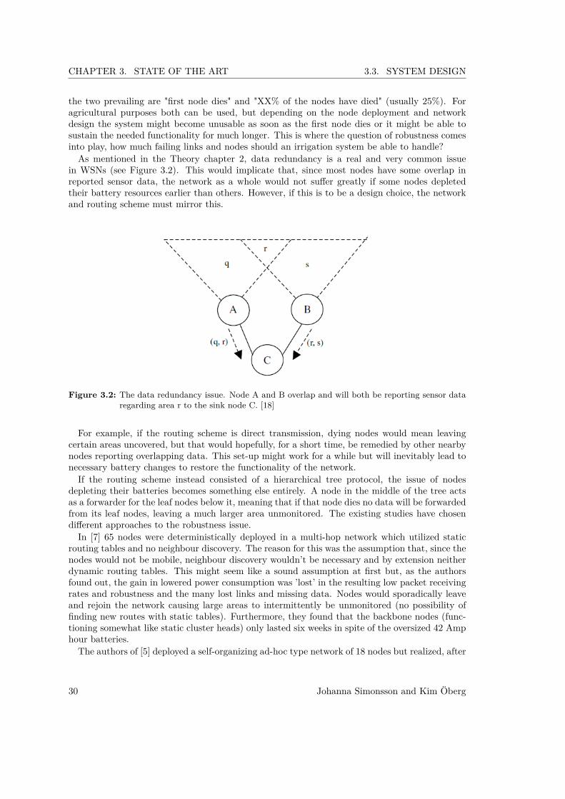
CHAPTER 3. STATE OF THE ART 3.3. SYSTEM DESIGN
the two prevailing are "first node dies" and "XX% of the nodes have died" (usually 25%). Foragricultural purposes both can be used, but depending on the node deployment and networkdesign the system might become unusable as soon as the first node dies or it might be able tosustain the needed functionality for much longer. This is where the question of robustness comesinto play, how much failing links and nodes should an irrigation system be able to handle?As mentioned in the Theory chapter 2, data redundancy is a real and very common issue
in WSNs (see Figure 3.2). This would implicate that, since most nodes have some overlap inreported sensor data, the network as a whole would not suffer greatly if some nodes depletedtheir battery resources earlier than others. However, if this is to be a design choice, the networkand routing scheme must mirror this.
Figure 3.2: The data redundancy issue. Node A and B overlap and will both be reporting sensor dataregarding area r to the sink node C. [18]
For example, if the routing scheme is direct transmission, dying nodes would mean leavingcertain areas uncovered, but that would hopefully, for a short time, be remedied by other nearbynodes reporting overlapping data. This set-up might work for a while but will inevitably lead tonecessary battery changes to restore the functionality of the network.If the routing scheme instead consisted of a hierarchical tree protocol, the issue of nodes
depleting their batteries becomes something else entirely. A node in the middle of the tree actsas a forwarder for the leaf nodes below it, meaning that if that node dies no data will be forwardedfrom its leaf nodes, leaving a much larger area unmonitored. The existing studies have chosendifferent approaches to the robustness issue.In [7] 65 nodes were deterministically deployed in a multi-hop network which utilized static
routing tables and no neighbour discovery. The reason for this was the assumption that, since thenodes would not be mobile, neighbour discovery wouldn’t be necessary and by extension neitherdynamic routing tables. This might seem like a sound assumption at first but, as the authorsfound out, the gain in lowered power consumption was ’lost’ in the resulting low packet receivingrates and robustness and the many lost links and missing data. Nodes would sporadically leaveand rejoin the network causing large areas to intermittently be unmonitored (no possibility offinding new routes with static tables). Furthermore, they found that the backbone nodes (func-tioning somewhat like static cluster heads) only lasted six weeks in spite of the oversized 42 Amphour batteries.The authors of [5] deployed a self-organizing ad-hoc type network of 18 nodes but realized, after
30 Johanna Simonsson and Kim Öberg

CHAPTER 3. STATE OF THE ART 3.3. SYSTEM DESIGN
having conducted in-depth ethnographic research, that this might not be the optimal choice. Asfuture work they suggested an architecture which would use data mules, meaning that the sensornodes would implement neighbour discovery and simply send the accumulated sensor data toa sink node attached to farming equipment or workers as they traverse the area. This way allnodes would save energy by transmitting seldom and only over short distances. However, thisapproach might not at all help the power consumption since this would force all nodes to idlelisten for long periods of time. Furthermore scarce monitoring might result in insufficient datafor precision agriculture.The tree topology is advocated only by the authors of [9] as a part of the MINT protocol.
However, those nodes only stayed active for 3 weeks on their original batteries.The only study that implemented a self-healing robust system was [6]. The authors determin-
istically deployed 64 TelosB nodes covering an area of 0.5 hectare, which utilized a self-healingmulti-hop architecture. In comparison to the other studies performed very few issues arose dueto system robustness or power consumption with this approach. The authors conclude that theaverage overhead for the communication is quite low compared to achieved robustness: 56 bytesper transmission round. This would indicate that the proposed savings in power, due to the staticrouting tables in [7], are negligible in comparison to the gains in robustness.As mentioned in the Theory chapter cluster based routing schemes are considered to be the
best in terms of robustness, scalability and power management but how well they perform istightly linked to how the cluster heads are chosen and their clusters are formed. At the forefrontof this are the authors of [59] who utilize multi-criterion optimization (MCOP) or multi-objectivedecision making, which is an engineering design method that deals with problems that have severalconflicting and possibly non-commensurable criteria which should be simultaneously optimized.Exactly how the MCOP is implemented and its benefits are explained in the following sections.
3.3.4 Cluster based routing schemesAs mentioned in the chapter 2 (Theory), there are a number of available routing schemes. Out ofthese, the cluster based approach has proven to be the most power efficient, robust and scalable[59] and is classified by the following criteria:
• Clustering method: distributed or centralized. A distributed approach means that eachnode makes its own decisions and calculations regarding whether to become cluster head(CH) and which cluster to belong to, as opposed to letting the central main frame make allof those decisions.
• Network architecture: single or multi-hop. Single-hop architectures make no use offorwarding or relaying of packets between nodes, whereas multi-hop do.
• Clustering objective: energy efficiency or coverage. Is the aim to lower power usage orto provide coverage? Each is chosen at the expense of the other.
• Cluster head selection method: random or deterministic. Random cluster head selec-tion (as in LEACH) means that the choices and parameters are local to each node. In otherwords, the effect on the system as a whole isn’t weighted in [61].
As this thesis focuses on a WSN meant for implementation within the area of irrigation, thefollowing characteristics are suitable:
• Clustering method: distributed.• Network architecture: multi-hop.• Clustering objective: energy efficiency.• Cluster head selection method: deterministic.
Johanna Simonsson and Kim Öberg 31
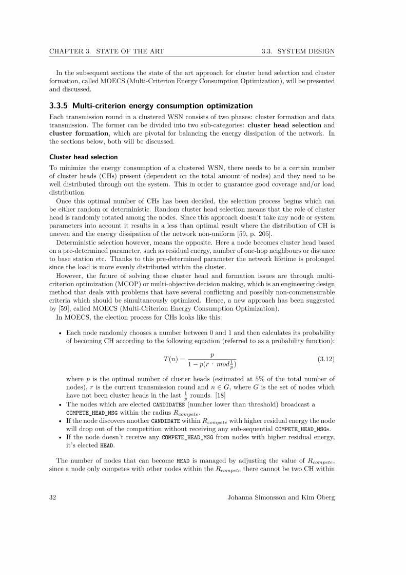
CHAPTER 3. STATE OF THE ART 3.3. SYSTEM DESIGN
In the subsequent sections the state of the art approach for cluster head selection and clusterformation, called MOECS (Multi-Criterion Energy Consumption Optimization), will be presentedand discussed.
3.3.5 Multi-criterion energy consumption optimizationEach transmission round in a clustered WSN consists of two phases: cluster formation and datatransmission. The former can be divided into two sub-categories: cluster head selection andcluster formation, which are pivotal for balancing the energy dissipation of the network. Inthe sections below, both will be discussed.
Cluster head selectionTo minimize the energy consumption of a clustered WSN, there needs to be a certain numberof cluster heads (CHs) present (dependent on the total amount of nodes) and they need to bewell distributed through out the system. This in order to guarantee good coverage and/or loaddistribution.Once this optimal number of CHs has been decided, the selection process begins which can
be either random or deterministic. Random cluster head selection means that the role of clusterhead is randomly rotated among the nodes. Since this approach doesn’t take any node or systemparameters into account it results in a less than optimal result where the distribution of CH isuneven and the energy dissipation of the network non-uniform [59, p. 205].Deterministic selection however, means the opposite. Here a node becomes cluster head based
on a pre-determined parameter, such as residual energy, number of one-hop neighbours or distanceto base station etc. Thanks to this pre-determined parameter the network lifetime is prolongedsince the load is more evenly distributed within the cluster.However, the future of solving these cluster head and formation issues are through multi-
criterion optimization (MCOP) or multi-objective decision making, which is an engineering designmethod that deals with problems that have several conflicting and possibly non-commensurablecriteria which should be simultaneously optimized. Hence, a new approach has been suggestedby [59], called MOECS (Multi-Criterion Energy Consumption Optimization).In MOECS, the election process for CHs looks like this:
• Each node randomly chooses a number between 0 and 1 and then calculates its probabilityof becoming CH according to the following equation (referred to as a probability function):
T (n) = p
1− p(r·mod 1p )
(3.12)
where p is the optimal number of cluster heads (estimated at 5% of the total number ofnodes), r is the current transmission round and n ∈ G, where G is the set of nodes whichhave not been cluster heads in the last 1
p rounds. [18]• The nodes which are elected CANDIDATES (number lower than threshold) broadcast a
COMPETE_HEAD_MSG within the radius Rcompete.• If the node discovers another CANDIDATE within Rcompete with higher residual energy the node
will drop out of the competition without receiving any sub-sequential COMPETE_HEAD_MSGs.• If the node doesn’t receive any COMPETE_HEAD_MSG from nodes with higher residual energy,
it’s elected HEAD.
The number of nodes that can become HEAD is managed by adjusting the value of Rcompete,since a node only competes with other nodes within the Rcompete there cannot be two CH within
32 Johanna Simonsson and Kim Öberg
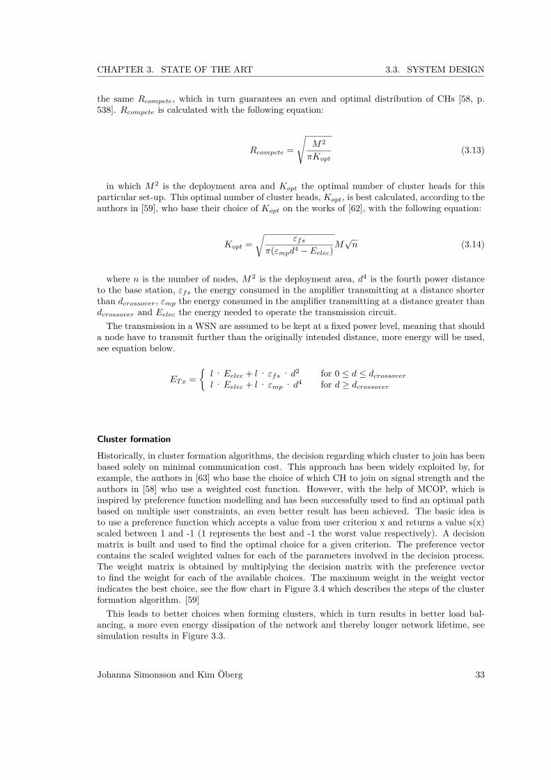
CHAPTER 3. STATE OF THE ART 3.3. SYSTEM DESIGN
the same Rcompete, which in turn guarantees an even and optimal distribution of CHs [58, p.538]. Rcompete is calculated with the following equation:
Rcompete =
√M2
πKopt(3.13)
in which M2 is the deployment area and Kopt the optimal number of cluster heads for thisparticular set-up. This optimal number of cluster heads, Kopt, is best calculated, according to theauthors in [59], who base their choice of Kopt on the works of [62], with the following equation:
Kopt =√
εfsπ(εmpd4 − Eelec)
M√n (3.14)
where n is the number of nodes, M2 is the deployment area, d4 is the fourth power distanceto the base station, εfs the energy consumed in the amplifier transmitting at a distance shorterthan dcrossover, εmp the energy consumed in the amplifier transmitting at a distance greater thandcrossover and Eelec the energy needed to operate the transmission circuit.The transmission in a WSN are assumed to be kept at a fixed power level, meaning that should
a node have to transmit further than the originally intended distance, more energy will be used,see equation below.
ETx ={l·Eelec + l· εfs · d2 for 0 ≤ d ≤ dcrossoverl·Eelec + l· εmp · d4 for d ≥ dcrossover
Cluster formation
Historically, in cluster formation algorithms, the decision regarding which cluster to join has beenbased solely on minimal communication cost. This approach has been widely exploited by, forexample, the authors in [63] who base the choice of which CH to join on signal strength and theauthors in [58] who use a weighted cost function. However, with the help of MCOP, which isinspired by preference function modelling and has been successfully used to find an optimal pathbased on multiple user constraints, an even better result has been achieved. The basic idea isto use a preference function which accepts a value from user criterion x and returns a value s(x)scaled between 1 and -1 (1 represents the best and -1 the worst value respectively). A decisionmatrix is built and used to find the optimal choice for a given criterion. The preference vectorcontains the scaled weighted values for each of the parameters involved in the decision process.The weight matrix is obtained by multiplying the decision matrix with the preference vectorto find the weight for each of the available choices. The maximum weight in the weight vectorindicates the best choice, see the flow chart in Figure 3.4 which describes the steps of the clusterformation algorithm. [59]This leads to better choices when forming clusters, which in turn results in better load bal-
ancing, a more even energy dissipation of the network and thereby longer network lifetime, seesimulation results in Figure 3.3.
Johanna Simonsson and Kim Öberg 33

CHAPTER 3. STATE OF THE ART 3.3. SYSTEM DESIGN
Figure 3.3: Network life in rounds for: (a) random topology 200 nodes, (b) random topology 500 nodes,(c) grid topology 100 nodes and (d) grid topology 400 nodes. [59]
As can be seen in Figure 3.3 a) and b) demonstrate the results for randomly deployed nodeson an area of 100 x 100 meters and c) and d) the results from a grid topology (more interestingfrom an agricultural point of view).In a) and b) the first node death occurs after 920 and 980 rounds respectively and under this
criterion MOECS extends the network lifetime with approximately 10 % compared to EECS,25% compared to LEACH and 200% compared to HEED. In c) and d) the results are similar.But if the first node death is substituted for 20% and 50% dead nodes, the results for HEED
are actually comparable to MOECS under large node densities.In other words, MOECS is the now reigning cluster based protocol showing the best perfor-
mance. However, worth noticing is that the research on MOECS was first published in 2008, i.e.after many of the mentioned studies on WSN and irrigation had been made. The only study tobe released afterwards, in 2010, is [6] in which the use of a much more primitive cluster basedalgorithm is explored.
34 Johanna Simonsson and Kim Öberg

CHAPTER 3. STATE OF THE ART 3.3. SYSTEM DESIGN
Figure 3.4: The cluster formation algorithm in MOECS [59].
Johanna Simonsson and Kim Öberg 35

CHAPTER 3. STATE OF THE ART 3.3. SYSTEM DESIGN
3.3.6 Power mode handlingApart from the power consumption of the network, the power consumption for the MCU isimportant to consider. The power consumption for a MCU can be divided into two categories,the power consumed while being a) Active, b) Idle. Easily put, active is when the MCU havetasks to execute, and idle is when the MCU waits for new tasks. If, for example, the currentconsumption of the MSP430, a commonly used MCU for wireless sensor nodes [64], is studied,see Table I, the difference is easily observed. The technique of choosing the correct power statefor an MCU while being idle is called Power Mode Handling.
Table I: Nominal current consumption by a TI MSP430f2617 microcontroller. [27]Power State CurrentActive Mode at 16MHz < 10mAActive Mode at 1MHz 0.5mAStandby Mode 0.5µAOFF Mode 0.1µA
To save energy when the node is not performing any tasks, the MCU have to make sure theprocessor uses the correct power mode when being idle. For example, as can be seen in Table II,the MSP430 uses less clock and oscillator modules if the power mode is lowered. As the authors of[65] and [66] explains, an algorithm which can determine the optimal power mode for a thresholdtime t is therefore needed in systems that want to decrease the total power consumption.
Table II: Clocks on/off in different Low Power Modes for MSP430f2617 [67]Mode Active LPM0 LPM1 LPM2 LPM3 LPM4CPU On Off Off Off Off OffMCLK On On Off Off Off OffSMCLK On On On Off Off OffDCO On On On On Off OffALCK On On On On On OffCrystal Oscillator On On On On On On
The first energy cost to take in account when deciding if a device should change its powermode, is the cost of power when transitioning. To justify a transition on the MSP430f2617microcontroller (see Table I) between, for example, the two states active and standby, the energysaved in the standby state should exceed the power-up cost to the active state. The energycost when transitioning the other way around, from active to standby is in comparison oftenmuch lower, and will therefore be neglected in the following equations. Let tstandby denote thetime the device stays in standby state, and Pstandby be the power consumption in standby. Thetransition time between standby and active is denoted as ts,a, and the power consumed is definedas Ps,a. Lastly, the power that the active state consumes is denoted as Pactive. Hence, to justifya transition, as [68] explains, the following equation should be fulfilled:
Pstandby · tstandby + Ps,a · ts,a ≤ Pactive · (tstandby + ts,a). (3.15)The time spent in standby, tstandby, is justified if
tstandby ≥ max(
0, (Pactive − Ps,a) · ts,aPstandby − Pactive
)(3.16)
36 Johanna Simonsson and Kim Öberg

CHAPTER 3. STATE OF THE ART 3.3. SYSTEM DESIGN
The active and standby state can be generalized as a transition between any state i (any higheroperating mode) and j (any lower operating mode),
tj ≥ max(
0, (Pi − Pj,i) · tj,iPj − Pi
). (3.17)
If the transition costs is the same moving from higher to lower as the opposite, the energysaved can be expressed as
Esaved,j = Pi · (tj + ti,j + tj,i)−(Pi + Pj
2
)(ti,j + tj,i)− (Pi − Pj) · tj . (3.18)
This means that the power can be decreased by increasing the gap between Pi and Pj , increasingthe time tj spent in state j, or decreasing the transition times.The authors of [69] argued that an important aspect when scheduling which power mode the
processor should enter is to evaluate when or if it should enter the lowest sleep state. This stateoften has all excess functions off, like the sensor, transceiver and ADC circuits. This means thatthe only way to wake the node up is to have a scheduled internal interrupt. If the lowest sleepstate is used, the program needs to know when the next event is happening, with two approachesto take in consideration. The node can wake up more a bit more often than it should, and riskunnecessary idle time, or wake up less often and risk missing events. The choice is of coursebased on the system design.
Active modeApart from optimizing the power consumption when the node is idle, the power consumptionwhen the node is active can be considered. The relationship between power P and speed s of aprocessor is often denoted as
P (s) = sα (3.19)
where α > 1 and constant. Equation (3.19) is based on the well-known cube-root rule, whichspecifies that all in CMOS-based processors, the power is proportional or equivalent to s3. Thisphenomena can be observed in Table I. The preferred implementation is therefore to run theCPU at the lowest possible speed setting whenever possible. A speed-scaling problem arises ifthe deadlines of the task being executed are strict, and can be solved with a technique calledDynamic Frequency Scaling, or DFS [70].
Johanna Simonsson and Kim Öberg 37

CHAPTER 3. STATE OF THE ART 3.4. THE INTERNET OF THINGS
3.4 The Internet of ThingsBeyond the deployment, topology and routing scheme choices listed in the previous sections liesanother big decision, whether to construct a so called online irrigation system, meaning whetherto have the nodes talk IP or not. The implications of a transition towards an online system willbe presented in this section.
3.4.1 The history of Internet of Things
The ability to connect smart embedded objects to the Internet is what is normally referred toas the Internet of Things. However, this transition from "offline" sensor networks to Internetconnected networks introduces a number of challenges, all related to successfully porting theuse of Internet technologies onto small, low cost, constrained units with limited power, memoryand processing power. Furthermore, these embedded devices and their networks display verydifferent characteristics than their big brothers operating in today’s Internet: their traffic patternis different, they suffer from high packet loss, low throughput and frequent topology changes andutilize small useful payload sizes. [71]
There have been several attempts at creating an extension of the Internet to constraineddevices in the past few years. But all of them, up until recently, have resulted in proprietaryprotocols making the interoperability of these vendor-specific Internet-enabled devices impossible,since the connectivity in these networks is achieved through vendor-specific gateways or proxies.Furthermore, with these proprietary protocols the user can only communicate with the nodesthrough a gateway or proxy that acts as a translator. This solution offers little to no flexibilityas the user can only query the sensors according to the API provided by the gateway. On top ofthat, the use of proprietary protocols means gateways and sensors need to be of the same brandin order to function together. [71]
These limitations combined with the curiosity and newly discovered potential of an Internet ofThings led to the IETF (Internet Engineering Task Force) initiative [71] to form the 6LoWPAN(IPv6 over Low Power WPAN ), ROLL (Routing Over Low Power and Lossy Networks) andCoRE (Constrained Restful environments) working groups, all with the aim of producing a non-proprietary solution, interoperable with the most widely used protocols of the Internet, IP, theInternet Protocol.
The 6LoWPAN group tackles the transmission of IPv6 packets over IEEE 802.15.4 networks,the ROLL group develops routing solutions for LLNs (Low Power and Lossy Networks), of whichIEEE 802.15.4 networks are a part, and the CoRE group provides a framework for resource-oriented applications intended to run on constrained IP networks. Together, these protocols,frameworks and solutions allow small constrained networks to run the Internet Protocol in astandardized way. [71]
3.4.2 IEEE 802.15.4 networks
In the subsequent sections, the IEEE 802.15.4 standard, a well known WSN standard, and itslayers will be presented.
In order to facilitate the explanation of these concepts, the OSI model, see Figure 3.5, willbe presented first to help with an overview of where in the communication model the differentstandards and protocols operate.
38 Johanna Simonsson and Kim Öberg
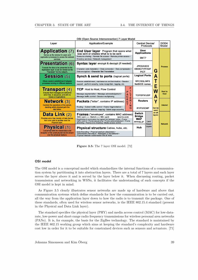
CHAPTER 3. STATE OF THE ART 3.4. THE INTERNET OF THINGS
Figure 3.5: The 7 layer OSI model. [72]
OSI model
The OSI model is a conceptual model which standardizes the internal functions of a communica-tion system by partitioning it into abstraction layers. There are a total of 7 layers and each layerserves the layer above it and is served by the layer below it. When discussing routing, packettransmission and networking in WSNs, it facilitates the understanding of such concepts if theOSI model is kept in mind.
As Figure 3.5 clearly illustrates sensor networks are made up of hardware and above thatcommunication systems which define standards for how the communication is to be carried out,all the way from the application layer down to how the radio is to transmit the package. One ofthese standards, often used for wireless sensor networks, is the IEEE 802.15.4 standard (presentin the Physical and Data Link layer).
The standard specifies the physical layer (PHY) and media access control (MAC) for low-data-rate, low-power and short-range radio frequency transmissions for wireless personal area networks(PANs). It is, for example, the basis for the ZigBee technology. The standard is maintained bythe IEEE 802.15 working group which aims at keeping the standard’s complexity and hardwarecost low in order for it to be suitable for constrained devices such as sensors and actuators. [71]
Johanna Simonsson and Kim Öberg 39

CHAPTER 3. STATE OF THE ART 3.4. THE INTERNET OF THINGS
Physical layer
The physical layer of the IEEE 802.15.4 standard controls the activation/deactivation of theradio transceiver, data reception/transmission, channel frequency selection and channel energydetection and is also responsible for checking whether the communication channel is occupied bya transmission or not, referred to as Clear Channel Assessment (CCA).The communication range for 802.15.4 devices spans from 10 to 100 meters depending on the
physical layer mode (the standard defines as many as 15 PHY modes) and the environment.Communication is achieved by radio transmission at one of the following license-free bands: 868-868.6 MHz (Europe), 902-928 MHz (North America) or 2400-2483.5 MHz (ISM band).
Media Access Control
When a device wants to send a packet it needs a means of knowing whether the other device isready to receive said packet or not, this is where the MAC layer comes into play. It manages theaccess of the physical channel and requests a CCA check before allowing a packet to be sent. Ifthe CCA indicates a transmission is taking place, the MAC postpones the transmission for a setamount of time before trying again. If no transmission is taking place when the CCA check ismade, the MAC transmits the packet immediately.Apart from the management of the physical layer the MAC also provides acknowledgement
of frame reception and validation of incoming frames. Furthermore it natively supports threenetwork topologies: star, mesh and cluster tree. But these are rarely used in practise as mostprotocols which build upon the IEEE 802.15.4 standard define their own networks instead.Duty cycles are also managed in the MAC layer with the result that transceivers can be in
sleeping mode up to 99% of the time, leading to a drastically improved network lifetime. [71]
Transport layer
The transport layer are responsible for the end-to-end communication over the network andbreaking the message up into smaller segments to pass them on to the network layer. To makesure the quality and reliability are maintained for the end user, it also handles error management.This means that the transport layer provides a few different services like Connection-orientedcommunication, which refers to the technique where the hosts involves ensures that the connectionis robust enough before sending the packet. This involves ’handshaking’ which means sendingacknowledgements before setting up the connection and making sure the packet arrives in thecorrect sequence. The transport layer also have services referring to Reliability, for exampleerror detection can be implemented in the form of checksum to make sure data is not corrupted.Another service is Flow Control, which means making sure the data stream from an end devicematches the receiving device’s ability to buffer and process. If this does not work, the buffer onthe receiving end could overflow or underrun. Multiplexing is a service referring to multiplexingseveral packet streams from other sources. The two primary implementations of transport layerprotocols are Transmission Control Protocol, TCP, standard for the internet protocol stack andthe more simple User Datagram Protocol, UDP. [73]TCP is used when reliable and ordered communication is needed. The services include error-
checked delivery, flow control and connection-oriented communication through handshaking. [74]UDP are more simple TCP, and focuses on transmission rather than security. This means no
handshaking or such, which means UDP cannot ensure delivery or avoiding duplication. However,by not implementing these feature UDP minimizes the packet overhead compared to TCP. [75]
40 Johanna Simonsson and Kim Öberg
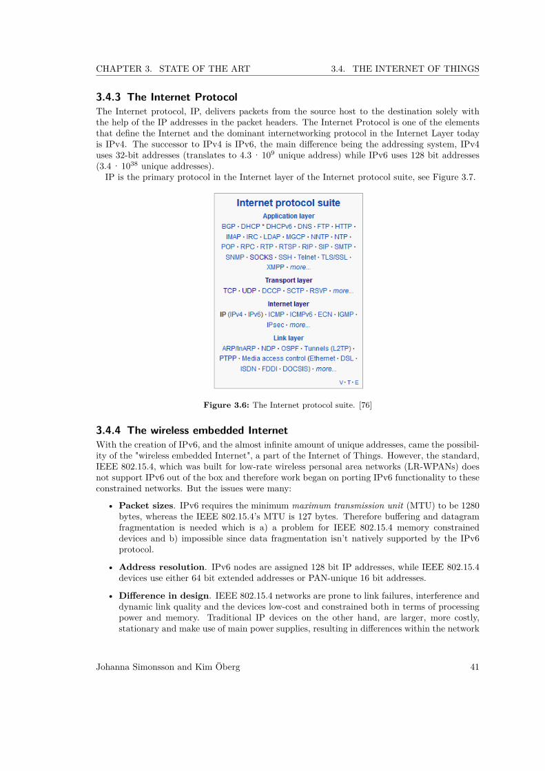
CHAPTER 3. STATE OF THE ART 3.4. THE INTERNET OF THINGS
3.4.3 The Internet ProtocolThe Internet protocol, IP, delivers packets from the source host to the destination solely withthe help of the IP addresses in the packet headers. The Internet Protocol is one of the elementsthat define the Internet and the dominant internetworking protocol in the Internet Layer todayis IPv4. The successor to IPv4 is IPv6, the main difference being the addressing system, IPv4uses 32-bit addresses (translates to 4.3 · 109 unique address) while IPv6 uses 128 bit addresses(3.4 · 1038 unique addresses).IP is the primary protocol in the Internet layer of the Internet protocol suite, see Figure 3.7.
Figure 3.6: The Internet protocol suite. [76]
3.4.4 The wireless embedded InternetWith the creation of IPv6, and the almost infinite amount of unique addresses, came the possibil-ity of the "wireless embedded Internet", a part of the Internet of Things. However, the standard,IEEE 802.15.4, which was built for low-rate wireless personal area networks (LR-WPANs) doesnot support IPv6 out of the box and therefore work began on porting IPv6 functionality to theseconstrained networks. But the issues were many:
• Packet sizes. IPv6 requires the minimum maximum transmission unit (MTU) to be 1280bytes, whereas the IEEE 802.15.4’s MTU is 127 bytes. Therefore buffering and datagramfragmentation is needed which is a) a problem for IEEE 802.15.4 memory constraineddevices and b) impossible since data fragmentation isn’t natively supported by the IPv6protocol.
• Address resolution. IPv6 nodes are assigned 128 bit IP addresses, while IEEE 802.15.4devices use either 64 bit extended addresses or PAN-unique 16 bit addresses.
• Difference in design. IEEE 802.15.4 networks are prone to link failures, interference anddynamic link quality and the devices low-cost and constrained both in terms of processingpower and memory. Traditional IP devices on the other hand, are larger, more costly,stationary and make use of main power supplies, resulting in differences within the network
Johanna Simonsson and Kim Öberg 41

CHAPTER 3. STATE OF THE ART 3.4. THE INTERNET OF THINGS
layer, which in IEEE 802.15.4 is required to be responsive and adaptive while still remainingenergy efficient.
• Routing and mesh topologies. Routing is a two phased problem for IP-based IEEE802.15.4 networks. Firstly, IEEE 802.15.4 does not natively support mesh topologies (multi-hop) which is common both in the IP domain and within normal IEEE 802.15.4 networks.Secondly IP routing is typically done by storing the IPv6 destination and next hop addressesin the routing headers which requires 32 bytes of memory, a solution which is impossibleon constrained low-memory devices. [77]
These issues were addressed by the IETF 6LoWPAN working group and resulted in the de-velopment of the 6LoWPAN Adaptation Layer, which successfully ports the IPv6 technology toIEEE 802.15.4 low-cost and constrained networks.
3.4.5 6LoWPAN6LoWPAN stands for IPv6 over Low power Wireless Personal Area Networks and is the net-working technology that allows IPv6 packets to be carried efficiently within small link layer framessuch as those used by IEEE 802.15.4. How this is done is presented in the sections below.
Packet sizes and header compressionIPv6 forwarding routers do not support packet fragmentation, which means that communicatinghosts have to send packets with the right size (MTU). Since the IPv6 MTU of 1280 bytes issignificantly larger than the IEEE 802.15.4 defined MTU of 127 bytes, a way of successfullytransmitting these large IPv6 packets over IEEE 802.15.4 networks was needed.6LoWPAN solves this by introducing a layer between the network and data link layer (see
OSI-model in Figure 3.5) called the 6LoWPAN Adaptation Layer which provides the following:packet fragmentation and reassembly, header compression and data link layer routing, whichmeans that the multi-hop relaying of fragmented datagrams is taken care of in the second layerof the OSI-model (the data link layer). [71, 77]
Routing and mesh topologiesTo solve the issues related to routing, the 6LoWPAN Adaptation Layer supports routing both inthe link layer (layer two) and network layer (layer three). This is referred to as ’mesh under’ and’route over’ routing respectively.In the mesh under set-up, no IP routing is performed in the network layer. Instead the
6LoWPAN Adaptation Layer masks the lack of a full broadcast at the physical layer, therebyemulating a full broadcasting link and compatibility with IPv6 protocols.When utilizing a route over set-up however, all routing is performed in the IP layer, effectively
turning each node into a IP router. This mode supports layer three forwarding mechanismswhich can utilize network layer capabilities defined by IP, such as IPv6 routing or hop-by-hopoption headers. Furthermore, route over constrains the IP communication to local radio coverageinstead of the entire LoWPAN (as in mesh under). [71, 77]
3.4.6 Routing over 6LoWPANSince the specification of 6LoWPAN, routing has been one of the key issues and there have beenattempts at specifying an efficient routing algorithm for 6LoWPAN-compliant IEEE 802.15.4networks, such as Hydro, Hilow and Dymo-low. However, these proprietary solutions did notgain much momentum. Instead, a non-proprietary routing protocol, referred to as RPL and
42 Johanna Simonsson and Kim Öberg
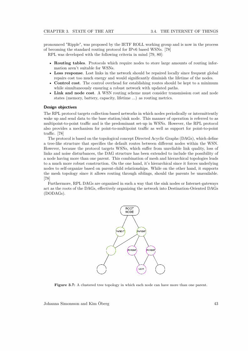
CHAPTER 3. STATE OF THE ART 3.4. THE INTERNET OF THINGS
pronounced "Ripple", was proposed by the IETF ROLL working group and is now in the processof becoming the standard routing protocol for IPv6 based WSNs. [78]RPL was developed with the following criteria in mind [79, 80]:
• Routing tables. Protocols which require nodes to store large amounts of routing infor-mation aren’t suitable for WSNs.
• Loss response. Lost links in the network should be repaired locally since frequent globalrepairs cost too much energy and would significantly diminish the lifetime of the nodes.
• Control cost. The control overhead for establishing routes should be kept to a minimumwhile simultaneously ensuring a robust network with updated paths.
• Link and node cost. A WSN routing scheme must consider transmission cost and nodestates (memory, battery, capacity, lifetime ...) as routing metrics.
Design objectivesThe RPL protocol targets collection-based networks in which nodes periodically or intermittentlywake up and send data to the base station/sink node. This manner of operation is referred to asmultipoint-to-point traffic and is the predominant set-up in WSNs. However, the RPL protocolalso provides a mechanism for point-to-multipoint traffic as well as support for point-to-pointtraffic. [78]The protocol is based on the topological concept Directed Acyclic Graphs (DAGs), which define
a tree-like structure that specifies the default routes between different nodes within the WSN.However, because the protocol targets WSNs, which suffer from unreliable link quality, loss oflinks and noise disturbances, the DAG structure has been extended to include the possibility ofa node having more than one parent. This combination of mesh and hierarchical topologies leadsto a much more robust construction. On the one hand, it’s hierarchical since it forces underlyingnodes to self-organize based on parent-child relationships. While on the other hand, it supportsthe mesh topology since it allows routing through siblings, should the parents be unavailable.[78]Furthermore, RPL DAGs are organized in such a way that the sink nodes or Internet-gateways
act as the roots of the DAGs, effectively organizing the network into Destination-Oriented DAGs(DODAGs).
Figure 3.7: A clustered tree topology in which each node can have more than one parent.
Johanna Simonsson and Kim Öberg 43

4 MethodThis section describes the engineering task of the Master Thesis, which consisted of comparingand evaluating possible hardware and software choices and constructing a functioning small scaleproof of concept system. In the sections below requirements, system design and componentchoices are presented.
4.1 RequirementsTo be able to answer the question: ”If a WSN, running an open-source operating system andcommunicating over 6LoWPAN, could be used in the field of autonomous irrigation?” and beforemaking any choices regarding the design of the proof of concept system, requirements engineeringwas performed in cooperation with the company representative Daniel Thysell. The aim was tocapture the most important functionality (according to the company) while still maintaining asystem design focus.Irrigation as well as precision agriculture systems today suffer from power optimization and
robustness issues. Therefore, these are the two main focuses through out all the design choices. Ifthe choice stands between implementing a feature that would cost the power budget the featureneed to be vital to the system or it will be discarded.These discussions and aims resulted in the requirements below, which are divided into two ar-
eas: hardware and system. The hardware requirements handles the constraints and requirementsimposed on the nodes and sensor, while the system requirements dictates minimum functionalityfor the network and back-end system.
Requirements
1. The sensor nodes shall1.1. be deterministically deployed.1.2. be able to read the soil moisture level.1.3. utilize two-way communication with the main frame.1.4. turn off redundant circuits when in idle mode.1.5. cost < € 1201.6. have a life span of at least 6 months.
2. The soil moisture sensor shall2.1. have a speed of measurement < 5 seconds.2.2. stay within 5% margin of error.2.3. cost < $ 100
3. The network shall3.1. be self-healing.3.2. utilize the 6LoWPAN protocol.
44

CHAPTER 4. METHOD 4.2. SYSTEM CONTROL LOOP
3.3. minimize communication overhead in the transport layer.3.4. be scalable (1-100 nodes).3.5. be able to handle movable nodes (neighbour discovery).
4. The back-end system shall4.1. collect and store weather data from a local weather service going back at least 1 week.4.2. store data from the sensor nodes going back at least 1 week.4.3. make decisions regarding irrigation based on collected data.4.4. depending on weather/sensor data decide on sleep intervals for the nodes.
Once these requirements were settled, the system design was determined and then the suitablechoices for hardware and software made.
4.2 System control loopAs mentioned in Section 2.2 and 3.3 power saving and robustness are two very important factorswhen designing an irrigation system. However, one is almost always chosen at the expense of theother, which makes it a balancing act in which all design decisions have to be carefully evaluated.The overall aim of the system design was, by combining a smart irrigation system (see Section
3.1) with the WSN’s dense monitoring (see Section 3.2.1), to create a closed loop system. Thereason for wanting to create a closed loop system was the hypothesis that such a system couldimprove the performance of existing WSN solutions, both in terms of power and robustness.Furthermore, it’s a rare approach (only a few existing solutions implement this [40]) in theexisting technology and therefore not very well explored.The aim of the feedback loop is to guarantee that an exact amount of water is dispersed and
not an approximate amount based on a less than ideal model of the cultivated area and neededirrigation.Existing weather based systems utilize what can be described as an open loop system, see Figure
4.1, in which the weather is used as input to the controller (which calculates the ET equations).However, the resulting soil moisture level is never confirmed (fed back into the system) or usedin the calculation. The dispersed water is solely based on an ideal model of ET which assumesheterogeneity across the irrigated area. Furthermore, possible disturbances (v) are not at allaccounted or compensated for.
Figure 4.1: Open loop system in which irrigation is pre-determined either based on weather or soilmoisture sensor data. [11]
Looking at the existing approaches on the market, and their shortcomings, it’s obvious thatthe closed loop approach is new, not very well explored and possibly the answer to some of the
Johanna Simonsson and Kim Öberg 45

CHAPTER 4. METHOD 4.3. NODE SPECIFICATIONS
drawbacks mentioned. In such a system, the actual soil moisture level would be fed back intothe system (via the sensor nodes) and used in conjunction with current weather data and the ETequation to determine how much and when irrigation is needed, see Figure 4.2.
Figure 4.2: Closed loop feedback system in which the actual soil moisture level is fed back into thesystem, compared to the theoretical moisture level (based on ET), transformed into thecorresponding irrigation needs and then evaluated against the current weather forecast.[11]
More specifically, this means that the risk for over- or under-watering is virtually eliminatedsince the actual soil moisture level continuously will be fed back into the system in order to adjustthe needed irrigation. On top of that irrigation can be avoided when precipitation is imminentand the soil moisture level high enough to wait for the rain.In the model in Figure 4.2 y is the actual soil moisture level (θ), r the desired soil moisture
level, e the difference between the two and u the resulting irrigation needs. The discrepancybetween the desired θ and measured θ (e) is then used as input to the regulator F which willcompute the resulting irrigation needs after looking at weather data. With this system design,the aim is to minimize water and power usage (since pumps won’t be used unless absolutelynecessary).It is this closed loop feedback system that acts as the foundation of all further design choices.
Choices that will be discussed, motivated and evaluated in the coming sections.
4.3 Node specificationsTo meet the requested specifications in the requirements, market research was conducted regard-ing both node software and hardware. As some hardware requirements limits software and viceversa (not all nodes support 6LoWPAN out of the box) these choices were made more or lesssimultaneously. But since the company requested an IPv6 compliant system, the software wasresearched first.
4.3.1 Software choicesThe choice of software for the physical system was heavily affected by the company’s profilewithin embedded systems and Internet of Things, as the core of IoT is IP compliant software. Aquick market survey was conducted, which narrowed down the available choices to Contiki andTinyOS. Both operating systems support 6LoWPAN by implementing their own version of the
46 Johanna Simonsson and Kim Öberg

CHAPTER 4. METHOD 4.3. NODE SPECIFICATIONS
uIP | micro IP stack, uIPv6 and BLIP respectively, but they differ in other areas. For a quickoverview of the core functionalities, see Table I below.
Table I: Comparison between Contiki and TinyOS.Evaluation criteria Contiki TinyOSLanguage C nesCConcurrency Multi-threaded Event-drivenPower management Sleep modes Sleep modesMultitasking Optional pre-emptive Non-pre-emptiveLinking Dynamic StaticSimulator COOJA TOSSIMActive community Yes Yes
The main differences between the two operating systems lies in the way they handle concur-rency.Contiki is written in C and has implemented so called protothreads, a stackless lightweight
thread which is a mix of features from both multi-threading and event-driven programming. Thekernel invokes the protothread of a process in responds to internal or external events, for examplea fired timer or incoming radio packets from a neighbour. These protothreads are cooperativelyscheduled which means that the process must always explicitly yield control back to the kernelat regular intervals. [81]TinyOS programs are built out of software components, some of which present hardware ab-
stractions. Components are connected to each other using interfaces. TinyOS provides interfacesand components for common abstractions such as packet communication, routing, sensing, ac-tuation and storage. While being non-blocking enables TinyOS to maintain high concurrencywith one stack, it forces programmers to write complex logic by stitching together many smallevent handlers. To support larger computations, TinyOS provides tasks, which are similar to adeferred procedure call and interrupt handler bottom halves. A TinyOS component can post atask, which the OS will schedule to run later. Tasks are non-preemptive and run in FIFO order.[82]Since the company had experience with Contiki from earlier projects, and TinyOS and Contiki
are so similar in performance, it was decided to go with Contiki. However, the implementedoperating system was TinyOS. Motivation for this switch is made in the Discussion, see Section8.3.1.
Simulation softwareIn order to implement and properly evaluate the behaviour of a routing protocol with a require-ment on scalability, three sensor nodes (as in the proof-of-concept system) won’t suffice. Thedifference in behaviour for two sensor nodes utilizing direct transmission or RPL will be minorand won’t provide any useful insight into the performance of the routing. Therefore, it wasdecided to utilize a simulation tool. With such a tool any number of nodes could be deterministi-cally deployed several meters apart, spanning a large are corresponding to an actual deploymentsite. Furthermore, metrics such as packet loss ratio, routing table overhead and communicationoverhead (for example) can easily be displayed, stored and analysed.The two simulators, COOJA and TOSSIM (Contiki and TinyOS respectively) have similar
functionalities but COOJA supplies a very user friendly GUI whereas TOSSIM is run throughthe Python interpreter. This helped COOJA’s case when choosing the operating system andensured a way of verifying scalability.
Johanna Simonsson and Kim Öberg 47

CHAPTER 4. METHOD 4.3. NODE SPECIFICATIONS
Furthermore, both COOJA and TOSSIM can be configured to run with hardware deployedcode specifically to verify that written code and solutions scale as expected. [83, 84, 85]Another advantage of COOJA is the fact that it enables cross-level simulation. That means
that the nodes tested in this environment can be analysed in three different ways: networking(or application) level, operating system level or machine code instruction level. This enables theuser to change the analysis approach of the system, optimizing the power savings and algorithmsof the final network [85].Due to issues that arose along the way, the simulating software was neither implemented or
used (See Section 8.3.3.
4.3.2 Routing protocol choiceWhen constructing a closed loop feedback system, as mentioned in Section 4.2, one of the firstthings to consider is the manner in which the sensor data will travel from the nodes to the back-end (controller). In Section 3.3.2 and 3.3.4 a cluster based routing scheme is proposed as the bestsolution.Since the task was not to build a routing protocol from scratch (see Section 1.4 Scope), two
TinyOS built-in routing protocols were chosen for evaluation, namely TinyRPL (clustered treeprotocol, see Section 3.4.6), and Active Message (direct transmission, see Section 2.2.5).TinyRPL is the better protocol as proven in Section 3.3.2 but since the first goal was to setup
the feedback loop, AM (Active Message) was implemented first since it seemed more straightforward. The aim was then to replace it with TinyRPL. A short comparison between the twoprotocols can be seen in Table II.
Table II: Routing Protocols implemented in TinyOS. [86][87]Evaluation criteria TinyRPL Active MessageCharacteristicsNetwork topology Tree StarRouting protocol Clustered tree Direct transmissionMax packet size(byte) 127 39Transport layer UDP UDP
RequirementsSelf-healing Yes No (not needed)6LoWPAN support Yes NoMinimize overhead Yes YesScalable (1-100) Yes Yes*Neighbour discovery Yes No***scalability depends on signal strength (i.e. hardware dependent).
**since no packets are forwarded neighbour discovery is unnecessary.
As can be seen in Table II, TinyRPL utilizes 6LoWPAN, and fulfils all the requirement specifiedfor the network. AM falls short on a few points, the most important ones being routing protocoland 6LoWPAN support.Once the feedback loop was constructed and it had been confirmed that data was traversing the
system as expected the choice was made to switch to TinyRPL. However, due to issues discussedin Section 8.1.3, this turned out to be impossible. The proof-of-concept therefore continued usingActive Message.
48 Johanna Simonsson and Kim Öberg

CHAPTER 4. METHOD 4.3. NODE SPECIFICATIONS
4.3.3 Hardware choicesThe hardware for large scale deployments of WSN should be low-cost, robust and support thecurrent state of the art operating systems. Since software at this point already had been chosen,the hardware choice was narrowed down to nodes that supported Contiki. However, there werestill 31 platforms to choose from. Since the company had worked with the Zolertia Z1 nodebefore and specifically in a related project the choice leaned heavily from the beginning towardschoosing those sensor nodes. However, a quick background study was conducted anyway in whichthe most popular and common sensor nodes were evaluated, Table III below.
Table III: Characteristics of the TMote Sky, IRIS and Z1 sensor nodes [27, 28, 29].Evaluation criteria TMote Sky/TelosB Crossbow IRIS Zolertia Z1ProcessorMCU TI MSP430F1611 Atmel ATmega1281 TI MSP430F2617VCC 1.8 ... 3.6 V 2.7 ... 3.6 V 2.1 ... 3.6 VFlash 48 kB 128 kB 92 kBRAM 10 kB 8 kB 8 kBADC 12 bit 10 bit 12 bitCurrent draw: Active 0.5 mA @ 1MHz 8 mA @ 4MHz 0.5 mA @ 1MHzCurrent draw: Sleep 2.6 uA 8 uA 0.5 uA
RF TransceiverRadio chip TI CC2420 Atmel RF230 TI CC2420Data rate 250 kbps 250 kbps 250 kbpsTransmission power 0 : –25 dBm 0 : –24 dBm 0 : –25 dBmTX range outdoors (0 dB) 125 m > 300 m 180 m (antenna)Current draw: RX 19.7 mA 16 mA 18.8 mACurrent draw: TX 17.4 mA @ 0dBm 17 mA @ 3dBm 17.4 mA @ 0dBmCurrent draw: Sleep 1 uA 1 uA < 1 uA
ElectromechanicalGPIO 16 pin 51 pin expansion 52 pinOnboard sensors 3 - 3Power supply AA/USB AA/USB AA/micro USBUser interface 1 button, 3 LEDs 3 LEDs 1 button, 3 LEDsCost € 77 € 85 € 95
As can be seen in III the sensor nodes do not differ much in actual hardware specifications.That together with the following facts:
• The MCU’s has an ultralow current draw and is specifically designed for low power purposes.[88]
• It has an integrated temperature sensor [27], which expands the available data input to theirrigation decision.
• The integrated battery pack, making it standalone.• It was readily availability online.• The MCU and RF transceiver (MSP430 and CC2420) are recurrent in the WSN field.
is why the Zolertia Z1 node was chosen.
Johanna Simonsson and Kim Öberg 49

CHAPTER 4. METHOD 4.3. NODE SPECIFICATIONS
4.3.4 Soil moisture sensorThe fully developed solutions for smart irrigation on the market are many, but as to the availabil-ity for soil moisture sensors are few. There are, however, several ways to measure the moisturein soil.
1. Electrical conductivity probe: The probe measures the electrical resistance betweentwo electrodes. Wet soil has better conductivity, and therefore a higher reading is achieved.The electrodes have direct contact with the soil, which makes them more sensitive to salinityand pH. There is a possibility for oxidation on the electrodes, so the probe needs regularmaintenance. The probe needs calibration in every new type of soil, this again caused bythe high sensitivity. Apart from these flaws, the probe is often cheap and easy to attainonline. [89]
2. Electrical resistance block: The block measures the conductivity in the soil, just likean electrical conductivity probe. The difference is that this sensor electrodes are embeddedin gypsum or sand-ceramic mixture. A case made of fiberglass or perforated metal is alsocommon. This makes the electrical resistance block much less sensitive to outer factors.[90]
3. The Fringe Capacitance Sensor: Consists of two electrodes separated by a dielectricmaterial, a material which works as an insulator, but can be polarized with an electricalfield. When a high oscillating frequency is applied between the electrodes and a resonancefrequency can be measured. This resonance frequency is proportional to the capacitance,which increases as dielectric constant (a soil property) changes as the moisture content ofthe soil increases. [91]
4. TDR: or a Time-Domain Reflectometer uses a short electromagnetic pulse along a conduc-tor, which reflects and is measured to determine the moisture level. The speed of the pulsedecreases as the dielectric constant changes and the moisture increases. The technique isexpensive, but provides high accuracy. [89]
Table IV: Characteristics of the VH400, Watermark and SEN0114 Soil Moisture Sensors [92, 93, 94]Evaluation Critera VH400 Watermark SEN0114Price $ 37.95 $ 38.00 $ 4.80Technology 4. 2. 1.Supply Voltage 3.3-20VDC AC 3.3V, 5VOutput Voltage 0-3V 0-3V 0∼4.2VCurrent Cons. <7mA - 35mAResponse Time 400ms 65s -Accuracy 2% at 25◦C - -
Moisture sensor choiceAs the supply of soil moisture sensors online were limited, the choice was decided between threedifferent probes, see Table IV. Unfortunately, the Watermark sensor, an electrical resistanceblock, required AC. This requirement was seen as too difficult to implement on the Z1, and theprobe was therefore rejected. Also, the readings for this probe took around 65 seconds before theinstrument would give accurate results, an unacceptable time frame.The price on the SEN0114 made it worth to consider even with the disadvantage of the prob-
ability of oxidation and needed calibration. However, due to the company’s previous encounterwith this kind of sensor, they recommended against it, as the output was too unreliable.
50 Johanna Simonsson and Kim Öberg

CHAPTER 4. METHOD 4.4. BACK END
The choice fell on the VH400, with good response time, within the price range and the bestdocumented current consumption.
4.4 Back endThe back end of the system needed to collect and store node and weather data, perform compu-tations on stored data, make decisions and instruct the sink node. The front end of the systemneeded easy access to database data and an easy and straight forward way of presenting thatdata. A number of different options were thereby recommended by an expertise within the com-pany, namely the MVC frameworks: Django (Python), CodeIgniter (PHP) and Ruby on Rails(Ruby).PHP was considered because of the IPv6 functionality. With PHP it’s easy to build a web
server which can communicate directly with the nodes over IP. But since the project participantsdidn’t have that language competence it was concluded that it would be too time consumingto implement and instead the choice was made to stick to Python but learn how to use theDjango framework. Furthermore, the company supervisor had extensive knowledge in Djangodevelopment.Django ships with a built in SQLite database (which is file-based) but can be configured for use
with for example MySQL (which is server-based). It also comes with a lightweight, standaloneweb server for development and testing. [95]
4.4.1 Database choicesSince Django ships with a filebased SQLite database, but can be configured with many otherdatabase management systems, the choice stood between using the default database or imple-menting something more robust and well used like MySQL, Oracle etc.However, since the aim of the thesis didn’t concern web servers, frameworks or databases it
was decided to go with the default SQLite while being fully aware of its shortcomings such as:
• It’s file based, meaning non-robust and non-flexible. When all data is stored locally on thehard drive it leaves the system vulnerable.
• It doesn’t scale well.
Johanna Simonsson and Kim Öberg 51

5 ImplementationThe proof of concept system was built to answer the question: ”If a WSN, running an open-sourceoperating system and communicating over 6LoWPAN, could be used in the field of autonomousirrigation?” and to implement the requirements and design features discussed in Chapter 4(Method). The purpose was to identify if the design choices were suitable for an actual im-plementation. The following sections in this chapter will review the choices made to finish theproduct.
5.1 Overall system designThe system consists of two sensor nodes, one sink node, a PC acting as the main frame and a soilmoisture sensor, as seen in Figure 5.1. The final layout were made to utilize the system controlloop discussed in Section 4.2. The implementation of each component will be reviewed in thefollowing sections.
Figure 5.1: Outline for the system.
5.1.1 Node designNode design refers to the software choices made to implement the features needed for the systemto perform the wanted tasks.
NetworkThe communication protocol that were chosen was the standard implementation in TinyOS calledActive Message. Active Message, or AM, is a single-hop, best-effort communication packets thatgenerates the node addresses from a pre-programmed node id. Therefore the node id of the sink
52

CHAPTER 5. IMPLEMENTATION 5.1. OVERALL SYSTEM DESIGN
node, which acts as a base station are to be pre-programmed into all the sensor nodes. The nodescommunicated with the sink node through unicast and vice versa, meaning no other than thedesignated receiver read the sent message.
Sensor nodeThe sensor nodes primary objective was to gather soil moisture data and forward it to themain computer frame. The decision making process can be observed in Figure 5.2. The timerwas set according to a predetermined sampling frequency. To make sure the node didn’t wasteany unnecessary energy, all peripheral components was shut off when the node was idle, i.eentered sleep mode. One of the main power reduction techniques for MCU is shutting off thecomponents that aren’t needed, and therefore the implementation of said technique is importantfor all systems trying to save power, see Section 3.3.6. As the system characteristics implies thatTsleep >> Tactive, the assumption was made that the system should enter the lowest power modepossible (see Equation 3.18).
Figure 5.2: The decision making process for a node.
The MCU in the Z1 node, MSP430, utilizes 5 different power modes, where the lower the powermode, the less clocks are turned on, see Table II. As the design utilizes a sleep timer for the nodeto wake up, the node needs to be able to receive an interrupt from a clock. The Auxiliary Clock,ALCK can be sourced from a 32kHz watch crystal, and is the only clock that is active in the LowPower Mode 3, LPM3, see Table II [67, p. 19]. Therefore the node sleep interval was decided bya timer that utilizes said 32kHz watch crystal. By calling the predefined API MCUSleep, whichevaluates how many of the peripheral components that are active and puts in the appropriatelow power mode, the node didn’t waste energy on components that weren’t used. As the systemdid not have any strict deadlines due to the characteristics of the system, the CPU were set atthe lowest available pre-defined speed at 1MHz. Another argument to use the lowest predefined
Johanna Simonsson and Kim Öberg 53

CHAPTER 5. IMPLEMENTATION 5.2. BACK-END FUNCTIONALITY
setting was due to the argument done in 3.3.6.
Soil moisture sensor
The soil moisture sensor utilized the 12-bit ADC conversion available on the MSP430 to convertthe input voltage from the VH400 to digital readings [67]. The voltage supply were Vcc+3V [92].The output given from the sensor were in the range of 0-3V, and could be recalculated to
soil moisture content θ by calibrating the sensor. However, the output voltage from VH400corresponding to θ is not linear, but can be converted depending on which segment the outputvalue corresponds to, see Table I.
Table I: Simulation results.Voltage Range Vout Equation for ε
0− 1.1V 10 ·Vout − 11.1V − 1.3V 25 ·Vout − 17.51.3V − 1.82V 48.08 ·Vout − 47.51.82V − 2.2V 26.32 ·Vout − 7.89
ε is the relative converted soil moisture value. After the conversion according to Table I, thesoil moisture could then be expressed as
θ = ε
εmax(5.1)
where εmax is maximum converted value when the soil is fully saturated.
Sink node
The purpose of the sink node was to gather the data from the sensor nodes and forward themessages to the main computer frame and vice versa. An illustration of the data flow is depictedin Figure 5.3. As the sink node was connected on the power grid through the main computerframe, there was no need to limit the functionality for power saving purposes. Therefore thelistening processes on both the UART and the radio was active at all times. This was also toprevent the system from losing any packets.
5.2 Back-end functionalityThe back-end system was run in an Ubuntu 12.04 Precise Pangolin environment upon whichTinyOS and Django have been installed. To integrate Ubuntu with the computers providedby the company, the operating system was installed using the open-source virtual environmentVirtualBox. The task of the back-end PC is to connect to a local weather service, download the5-day forecast, store it in a database, analyse it together with the collected and stored sensordata and then make decision on irrigation, see flowchart in Figure 5.4.
54 Johanna Simonsson and Kim Öberg

CHAPTER 5. IMPLEMENTATION 5.2. BACK-END FUNCTIONALITY
Figure 5.3: The decision making process for the sink node.
Figure 5.4: A flowchart of back-end code.
Johanna Simonsson and Kim Öberg 55

CHAPTER 5. IMPLEMENTATION 5.2. BACK-END FUNCTIONALITY
5.2.1 Database configurationDjango ships with a built in SQLite database in which tables were created with Django models.This meant creating classes in Django models which were then translated into SQL code whichultimately created the database structure, see Figure 5.5.
Figure 5.5: How Python code is translated into SQL by Django.
Django also automatically creates an admin interface on the web server, which allows the userto login with a created superuser account and then modify the content of the database tables bymanually adding data. This allows for early and continuous testing of the tables, data definitionsand general structure of the database, which was a great advantage. The final structure of thedatabase can be seen in Figure 5.6.
Figure 5.6: The structure for the Django created SQLite database.
5.2.2 Weather data collectionThe algorithm for the dynamic sleep intervals utilize weather data as a parameter when calculat-ing the length of the sleep periods. This meant creating a script which could connect to an online
56 Johanna Simonsson and Kim Öberg
CHAPTER 5. IMPLEMENTATION 5.2. BACK-END FUNCTIONALITY
weather service, download the data to an XML file, parse the file while scanning it for requesteddata and then put it in the Django database. Another calculation script would then query thedatabase, compute the needed variables and forward the information, via the sink node, to thesensor nodes.The weather script is written in Python, connects to yr.no and downloads the requested weather
data. Since the script needs to renew the downloaded weather data at a certain rate, to makesure calculations aren’t made on outdated information, cron was used to schedule the executionof the script. Cron is a time-based job scheduler which is native to Unix/Linux-based operatingsystems and thereby also to VirtualBox. The interval 24 hours was chosen since it was concludedthat weather forecasts, albeit unpredictable, don’t change fast enough to require more frequentmonitoring.The forecast service yr.no was used since it provides a very user friendly API for accessing and
downloading weather forecasts, namely in the form of a URL(http://www.yr.no/place/LOCATION/varsel.xml) in which LOCATION is simply replaced withthe desired location. Furthermore, the service is completely free and although there are limits tohow often data can be accessed and downloaded, those are much higher than the frequency ofdata updates needed for this thesis.The script used for querying the database and handling the communication with the sink node
was written in Java.
Johanna Simonsson and Kim Öberg 57

6 AnalysisWhen designing a complete and robust wireless sensor network, aimed at precision agriculture,specifically irrigation, there are, as shown in this report, many things to take into consideration.Out of all the different parameters to tweak and look further into, the following two have beenchosen for further analysis:
• Network design• Weather data usage
The following sections will go through the chosen approaches for the thesis and implementation,analyse the outcome and discuss the reliability of the methods used.
6.1 Network designAs mentioned in the Theory 2 chapter there are many aspects to take into account when designing,building and implementing a wireless sensor network aimed at precision agriculture, specificallyirrigation. Out of the literature and previous research done in the field ([7, 5, 6, 9, 54, 55])very few put much, if any, effort into the power management aspect of the network design.Furthermore, there is a trade-off between power management and robustness that for every givenWSN implementation needs to be addressed.As presented in the State of the Art chapter, the cluster based protocol MOECS is at the
forefront of robust and power aware routing. However, such an IPv6 compliant protocol has yetto be developed for IEEE 802.15.4 devices.Thence, this chapter will provide analytical test results from MATLAB-calculations based on
the First Order Radio model. The aim is to establish whether the MOECS protocol possiblycould outperform the TinyRPL protocol. Therefore both protocols are assumed to be sendingpackets of the same size in the following calculations (the MTU frame size of IEEE 802.4.15 whichis 127 octets).As mentioned in 4.3.1 (Method) simulations software should have been used for evaluation but
as discussed in 8.3.3 that was not possible. Furthermore, as discussed in 8.1.3 TinyRPL (theTinyOS implementation of RPL) could not be implemented due to hardware issues. Despite allthis there was still interest from the company to provide some kind of evaluation of the behaviourof TinyRPL, as it is the natural progression of the assembled proof-of-concept system (once thehardware has been replaced).
6.1.1 TinyRPL vs. MOECSAs mentioned in the Section 3.3.2 there exists a threshold at which a multi-hop architecturestarts to consume less power than direct transmission. In order to assess which type of protocolshould be used in terms of power consumption, a test bed was constructed and the followingassumptions made:Assumptions:
• All sensor nodes are stationary and homogeneous in terms of energy, communication andprocessing capabilities.
• Nodes are dispersed deterministically in a 2-dimensional space.
58

CHAPTER 6. ANALYSIS 6.1. NETWORK DESIGN
• The sink node is located outside the deployment region and has no energy constraints.• Nodes are location unaware i.e. they are not equipped with any GPS device.• Radios can expend the minimum energy to reach the intended recipients by controlling the
radio range.• Both protocols send packets of the same size: the MTU of the IEEE 802.15.4 standard, 127
octets.• The connectivity between nodes are uniform, meaning the link quality from A to B is equal
to that between B and A.• The First Order Radio model is used to calculate the dispensed energy.
With these assumptions and the requirements in Section 4.1 in mind, the following test bedwas constructed:
• 64 sensor nodes• 1 sink node• All sensor nodes were uniformly deployed in a grid pattern, 8 x 8• The inter-node distances was 10 meters• The entire area covered was 0.5 hectare land
The reason for choosing ∼ 60 nodes 10 meters apart stems from the earlier research conductedin [6, 7, 5, 9, 55], according to which a large WSN deployment correlates to ∼ 60 nodes. The onlyexisting larger test bed is the LOFAR-agro project which deployed 110 nodes, spaced approx 15meters apart, covering approximately 2.25 hectare land.Regarding the inter-node distances, the choice of 10 meters is a result of the earlier work
conducted, such as in [6, 7, 5], in which a mean distance of about 10-15 meters was used. Thereason for the short distances was both the aim of dense monitoring (precision agriculture) butalso the fact that all earlier studies ran into quite heavy connectivity issues between nodes. Theexisting test bed is visualized in Figure 6.1.The first thing to conclude, was whether to exclude direct transmission as a viable option
(the protocol the small proof-of-concept system was using). As presented earlier in 3.3.2, directtransmission requires less energy than multi-hop if the following equation holds true:
Edirect < Emulti−hop (6.1)Eelec + εampn
2r2 < (2n− 1)Eelec + εampnr2 (6.2)
Eelecεamp
<nr2
2 (6.3)
Since the average distance between nodes in the test bed is 10 meters and the average hop-depth4 (see the test bed in Figure 6.1) the result will be the following:
50 · 10−9
100 · 10−12 <4 · 102
2 =⇒(((((500 < 200 (6.4)
In other words, direct transmission will cost more than multi-hop in the existing set-up. Theaim now is to compare the existing state of the art routing scheme for IPv6 compliant networks,TinyRPL, to the, not yet IPv6 compliant, protocol MOECS. Whether or not to adhere to thegrowing IPv6 standard within WSN is a decision that has to be made with the implementationin mind. Needless to say, the possibilities are much greater when choosing an IPv6 compliantnetwork and routing protocol but might also cost the power budget. Normal packet-frames inTinyOS for AMpackets are 39 bytes, whereas the IPv6 packets are a whopping 127 bytes. Thatmeans that for transferring just one packet 10 meters, the consumed energy for sending the IPv6
Johanna Simonsson and Kim Öberg 59

CHAPTER 6. ANALYSIS 6.1. NETWORK DESIGN
Figure 6.1: The constructed test bed with 64 sensor nodes and 1 sink node, distributed in a 8 x 8uniform grid.
packet is almost 2.3 times larger than for the AM-packet (see Equation (3.2)). However, when thedistance is increased to 25 meters the consumed energy is 1.4 times larger than for AM-packets.So if the aim is simply to lower the power consumption it’s not certain that IPv6 is neces-
sary, depending on the distance the packets have to travel, as shown in Equation (3.2)) wherecommunication distance is the most important parameter.After having ruled out direct transmission, the two protocols were evaluated separately. A
cluster of 16 nodes in the south-west corner of the test bed was chosen for analysis.In the first scenario, concerning MOECS, see Figure 6.2, 15 nodes collect and send their data
to the CH which aggregates and forwards the data to the sink node. With the help of the firstorder radio model the resulting energy costs was calculated to 2.5161 mJ for the entire cluster,meaning 15 sending/receiving operations and one long distance transmission to the sink nodefrom the CH. The cost for a single packet to be transmitted from a node via the CH to the sinknode is 362.81 µJ.After having evaluated MOECS, a TinyRPL scenario was constructed, in which the path from
node to sink looked much different and includes more hops along the way, see Figure 6.3.The blue connections represents the one hop neighbour of each node in the tree and the red
thread a possible route through the tree structure in which each node transmits as far as it canreach in each step. With this approach the energy cost for one packet is 695.25 µJ and for allthe 16 nodes in the south west corner the cost would be 7.3353 mJ.
60 Johanna Simonsson and Kim Öberg

CHAPTER 6. ANALYSIS 6.1. NETWORK DESIGN
Figure 6.2: An example of 15 leaf node reporting their data to the current CH which in turn forwardsthe aggregated data, via another CH, to the sink node.
These preliminary results suggest that there are indeed power consumption improvements tobe made by switching to or implementing a clustered protocol over a tree protocol.
Table I: Simulation results.Scenario Cluster TreeTX/RX of 1 data packet 362.81 µJ 695.25 µJTX/RX of 16 data packets 2.5161 mJ 7.3353 mJ
As a comparison, the cost for 1 packet transmission in direct transmission is 828.04 µJ andfor a complete round of direct transmission for the entire test bed the total consumed energy is1.1355 J.These results and their reliability are discussed in Section 8.1.3.
6.1.2 Data aggregationIn both protocols mentioned above, data aggregation plays a big part in making the protocolefficient. Instead of simply forwarding the messages through the tree structure, each node addstheir own data as they forward the message to the sink. Same general idea goes for the clusterbased algorithm, in which the CH collects and aggregates the cluster data into one message whichis then transmitted to the sink.The interesting part becomes how to make sure unnecessary data isn’t appended to a message
or forwarded as a part of the CH message. Furthermore, both erroneous and redundant data
Johanna Simonsson and Kim Öberg 61

CHAPTER 6. ANALYSIS 6.1. NETWORK DESIGN
Figure 6.3: An example of a possible route through the network when utilizing a tree protocol.
must be avoided.For this, there are several approaches. The error and redundancy check can be made at the
sink, which has no power constraints and thus it won’t deplete the nodes’ energy. However, thecost for sending and receiving all the unnecessary data must then be taken into consideration. Asmarter approach, is the distributed one, in which each sensor node has an agent which locallysorts out the erroneous data and checks for data redundancy when adding data to a packet oraggregating cluster data. Furthermore, the agent limits the communication if only irrelevant datais present, thereby minimizing the communication costs.As always with WSNs, memory and processing power is limited and using the external flash
to store older measurements as comparison costs valuable energy.
62 Johanna Simonsson and Kim Öberg

CHAPTER 6. ANALYSIS 6.2. DYNAMIC SLEEP INTERVALS
6.2 Dynamic Sleep IntervalsAs mentioned in Section 3.1.1, most smart weather-based systems schedules irrigation by pre-dicting how much water will be depleted from the soil and then compensates that water losswith irrigation. This relationship between irrigation and water depletion, evapotranspiration, isexpressed in Equation (2.2). If a soil moisture sensor is used as well as weather data analysis,the initial values of ∆θ can be acquired, like the closed-loop solution suggested in Section 4.2.The sensors will also give feedback to the ET -calculations, so they can be validated [40]. If theirrigation is scheduled for a time t, and I0, R0 and θ0 is the values when t = 0 and I1, R1 and θ1is the values for t = T then:
θ1 − θ0
T= −ETC + I1 − I0
T+ R1 −R0
T, (6.5)
where the assumption that both rain R and irrigation I is added instantaneous is made. IfR = 0, I = 0 and ETC is constant, Equation (6.5) can be simplified and generalized for all t > 0as
θ1 = −ETC · t+ θ0. (6.6)
and visualized in figure 6.4. The soil moisture θ has to stay within the limits mentioned inEquation (2.5), where θMAD is the lower and θFC is the upper limit. If the system needs toirrigate every T to prevent the soil moisture target θ to reach the lower limit θMAD, the systemfrequency f can be assumed to be 1/T .
Figure 6.4: A simple representation on the relationship between soil moisture and time, affected byETC .
Johanna Simonsson and Kim Öberg 63
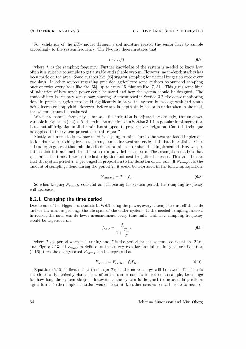
CHAPTER 6. ANALYSIS 6.2. DYNAMIC SLEEP INTERVALS
For validation of the ETC model through a soil moisture sensor, the sensor have to sampleaccordingly to the system frequency. The Nyquist theorem states that
f ≤ fs/2 (6.7)
where fs is the sampling frequency. Further knowledge of the system is needed to know howoften it is suitable to sample to get a stable and reliable system. However, no in-depth studies hasbeen made on the area. Some authors like [96] suggest sampling for normal irrigation once everytwo days. In other sources regarding precision agriculture some authors recommend samplingonce or twice every hour like the [55], up to every 15 minutes like [7, 51]. This gives some kindof indication of how much power could be saved and how the system should be designed. Thetrade-off here is accuracy versus power-saving. As mentioned in Section 3.2, the dense monitoringdone in precision agriculture could significantly improve the system knowledge with end resultbeing increased crop yield. However, before any in-depth study has been undertaken in the field,the system cannot be optimized.When the sample frequency is set and the irrigation is adjusted accordingly, the unknown
variable in Equation (2.2) is R, the rain. As mentioned in Section 3.1.1, a popular implementationis to shut off irrigation until the rain has stopped, to prevent over-irrigation. Can this techniquebe applied to the system presented in this report?Firstly, one needs to know how much it is going to rain. Due to the weather-based implemen-
tation done with fetching forecasts through an online weather service, this data is available. On aside note; to get real-time rain data feedback, a rain sensor should be implemented. However, inthis section it is assumed that the rain data provided is accurate. The assumption made is thatif it rains, the time t between the last irrigation and next irrigation increases. This would meanthat the system period T is prolonged in proportion to the duration of the rain. If Nsamples is theamount of samplings done during the period T , it could be expressed in the following Equation:
Nsample = T · fs. (6.8)
So when keeping Nsample constant and increasing the system period, the sampling frequencywill decrease.
6.2.1 Changing the time periodDue to one of the biggest constraints in WSN being the power, every attempt to turn off the nodeand/or the sensors prolongs the life span of the entire system. If the needed sampling intervalincreases, the node can do fewer measurements every time unit. This new sampling frequencywould be expressed as:
fnew = fs
1 + TRT
. (6.9)
where TR is period when it is raining and T is the period for the system, see Equation (2.16)and Figure 2.13. If Ecycle is defined as the energy cost for one full node cycle, see Equation(2.16), then the energy saved Esaved can be expressed as
Esaved = Ecycle · fsTR. (6.10)
Equation (6.10) indicates that the longer TR is, the more energy will be saved. The idea istherefore to dynamically change how often the sensor node is turned on to sample, i.e changefor how long the system sleeps. However, as the system is designed to be used in precisionagriculture, further implementation would be to utilize other sensors on each node to monitor
64 Johanna Simonsson and Kim Öberg

CHAPTER 6. ANALYSIS 6.2. DYNAMIC SLEEP INTERVALS
other environmental behaviours [7, 5]. If one were to implement a temperature sensor like [7], themeasurements would not be irrelevant during rain, and it might be difficult to motivate turningon the node less often when the period increases. However, the author of [97] states that it isthe sensors that consume the greatest portion of node energy, when the application is precisionagriculture. This means that it would still be a good idea to not utilize the soil moisture sensoras often as the other sensors when it is raining. This would be denoted as:
Esaved = Esoilsensor · fsTR. (6.11)
To make this work, the system needs to implement a feature that is not part of a normal multi-point-to-point communication routine: the main frame needs to be able to communicate back tothe node. The assumption is simple, if the power saved by extending the sampling intervals issurpassed by the power to communicate said change in sampling intervals, the transition is valid.If Ereceive is the energy cost for the system to send a message a specific node, change in samplingfrequency is motivated if:
Ereceive < Esaved. (6.12)
6.2.2 Taking precipitation into accountThe aim of implementing dynamic sleep intervals is tied to the idea that completely or partiallyturning off the sensor measurements and/or radio communication during rainy days could leadto significant improvement in battery lifetime.According to SMHI the average amount of days with more than 1 mm precipitation amounts
to ∼ 100 in Sweden [98]. As mentioned in the Section 6.2, Equation (6.10) dictates how muchenergy is saved during days when it’s raining. What it implies is that during rainy days thenumber of sampling actions are kept constant as the system’s time period increases, causing thesystem frequency to decrease, i.e. if rain is imminent 3 days ahead the periodicity of the systemincreases from 1 to 4 days but the number of sampling cycles remain the same and thus thefrequency changes. In practise this means that 3 days worth of sampling cycles are saved. So, ifit rains 100 days in a year the maximum save in energy is described by the following equation:
Esaved% = ���Ecycle ·��fs Train
���Ecycle ·��fs Tyear= 100
365 = 27.3%. (6.13)
6.2.3 ET dependent sleep intervalAs mentioned in 6.2.2 the aim is to have the sensor nodes adjust their sleep timers accordingto the weather, i.e. prolong the periodicity of the system during rain but keep the number ofsamplings constant (lower the frequency).This solution however, is constructed under the assumption that ET0 (and thereby the crop
specific ETC) is constant, resulting in the simplification of Equation (6.5) into Equation (6.6). Inother words, ET0 is calculated once, used as input and then never recalculated. This approachdoes not account for time dependent variations of ET0 and as a result the periodicity (T ) of thesystem is also considered static during non-rainy days.This translates to the linear relationship described in Figure 6.4, between θ (which depends
on ET0) and time. This relationship however, is quite misleading as the differences betweencalculating ET0 based on mean yearly, seasonally, monthly, weekly, daily or hourly values differgreatly. In areas where substantial changes in wind speed, dewpoint or cloudiness occur duringthe day, hourly calculations of ET0 are recommended [13]. This because such weather changes can
Johanna Simonsson and Kim Öberg 65

CHAPTER 6. ANALYSIS 6.2. DYNAMIC SLEEP INTERVALS
cause the daily average to misrepresent the evaporative power of the area and thereby introduceerrors into the calculations.
Figure 6.5: How the daily mean values for solar radiation, temperature and wind speed in Fort Laud-erdale, Florida, compare to the monthly averages. http://fawn.ifas.ufl.edu/data/reports/
As an illustration of these weather changes see Figure 6.5, in which it becomes clear how muchthe daily climatic data sometimes stray from the monthly average. Particularly the daily solarradiation values stray from the monthly average. But even the daily temperature average candiffer quite a lot from the monthly average. These discrepancies lead to the conclusion that thedaily ET0 value also differs somewhat from the monthly average. This relationship is presentedin Figure 6.6.As presented in Figure 6.6 the daily ET values can differ greatly from the monthly average and
particularly from the yearly. This implies that there are possible gains in power consumption tobe made by lengthening the periodicity of the system even on non-rainy days.However, which time step to use for the ET0 calculations depends on the purpose of the
calculation, the accuracy required and the time step of the climatic data available. ET0 is,as mentioned in 2.1, calculated with the help of climatic data. This implies that, in order toshorten the ET -calculation interval, that same data needs to be available for such short intervals.Thankfully today, with the advancement in meteorology, automation and electronics, leading toan increasing number of automated weather stations, such data is increasingly reported hourlyor with even shorter intervals. This hourly data together with automated ET calculations inirrigation systems, allows the Penman-Monteith equation to be re-calculated hourly, with goodresults. [13]Since the aim of this master thesis system is to, among others, prolong the network lifetime,
there is definitely motivation for computing ET on an hourly basis. Particularly since the main
66 Johanna Simonsson and Kim Öberg
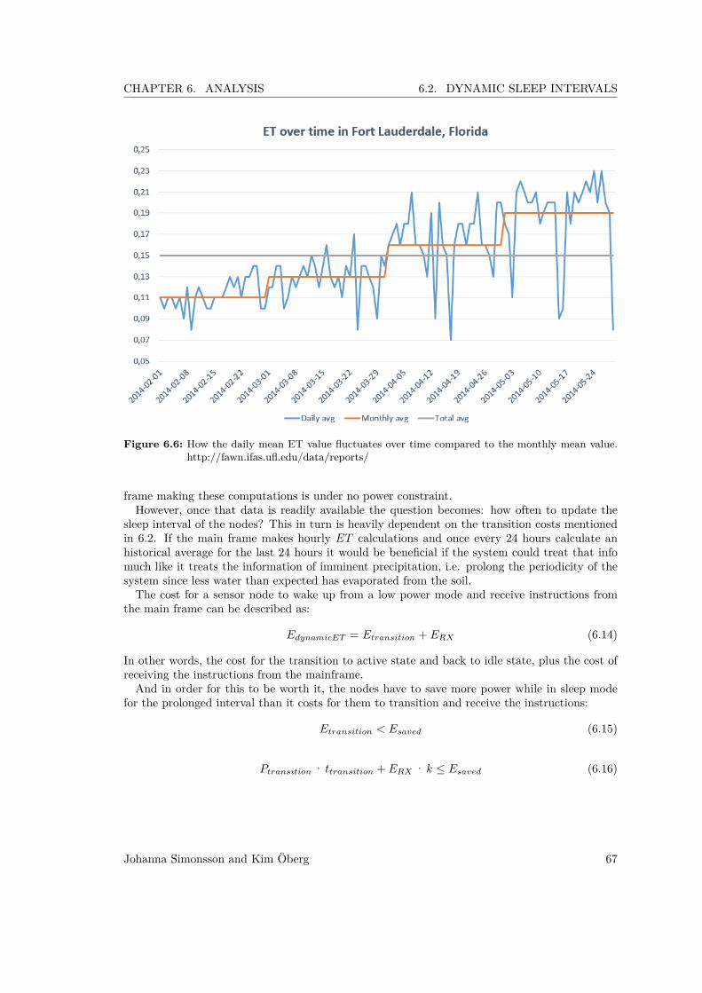
CHAPTER 6. ANALYSIS 6.2. DYNAMIC SLEEP INTERVALS
Figure 6.6: How the daily mean ET value fluctuates over time compared to the monthly mean value.http://fawn.ifas.ufl.edu/data/reports/
frame making these computations is under no power constraint.However, once that data is readily available the question becomes: how often to update the
sleep interval of the nodes? This in turn is heavily dependent on the transition costs mentionedin 6.2. If the main frame makes hourly ET calculations and once every 24 hours calculate anhistorical average for the last 24 hours it would be beneficial if the system could treat that infomuch like it treats the information of imminent precipitation, i.e. prolong the periodicity of thesystem since less water than expected has evaporated from the soil.The cost for a sensor node to wake up from a low power mode and receive instructions from
the main frame can be described as:
EdynamicET = Etransition + ERX (6.14)
In other words, the cost for the transition to active state and back to idle state, plus the cost ofreceiving the instructions from the mainframe.And in order for this to be worth it, the nodes have to save more power while in sleep mode
for the prolonged interval than it costs for them to transition and receive the instructions:
Etransition < Esaved (6.15)
Ptransition · ttransition + ERX · k ≤ Esaved (6.16)
Johanna Simonsson and Kim Öberg 67

7 ResultsIn this chapter the resulting proof-of-concept system and the internal information flow will bepresented.
7.1 Physical system overviewThe final physical system, upon which all software have been tested and developed, consists oftwo sensor nodes, one resistive moisture sensor and one sink node connected to a standard PCrunning Ubuntu through a VirtualBox installation, see Figure 7.1. The arrows back to the nodeindicate the two-way communication that was implemented to enable dynamically changing sleepintervals.
Figure 7.1: The final system with two-way communication implemented.
7.1.1 Node functionalityApart from the functionality implemented in Section 5, to fulfil the performance discussed inSection 6.2, the system needed to be able to:
• Have two-way communication between the sensor node and back-end system.• Dynamically change the sleep interval of the sensor node.
68

CHAPTER 7. RESULTS 7.1. PHYSICAL SYSTEM OVERVIEW
The two-way communication was simply implemented by letting the radio listen to incomingmessages for a set amount of time. The node started an alarm as soon as the sleep timer hadfired, which enabled listening after the node had sent the sensor data.The sleep intervals where updated by adjusting the periodic timer to the new value, as seen in
Algorithm 1.
if Message Received thenif NewSleepInterval != OldSleepInterval then
Update Periodic Timer with NewSleepInterval;end
endAlgorithm 1: Outline for updating the sleep interval for the node.
7.1.2 Back-end functionalityThe back-end system performed the task of calculating the new sleep interval for the sensornodes, and the new functionality can be observed in Figure 7.2 (the red text). The querying ofthe database and calculations for the sleep interval was done in a Java program. As soon as anode sent sensor values to the sink node which forwarded the sensor data to the back-end system,this Java program sent back the sleep interval right after the needed calculations were done. Thisto prevent the node for spending unnecessary time listening for a response.
Figure 7.2: A flowchart of back-end code that calculates new sleep intervals for the node.
Johanna Simonsson and Kim Öberg 69

CHAPTER 7. RESULTS 7.2. NODE LIFE SPAN
7.2 Node life spanSince power optimization is of great importance to WSNs, as discussed in Section 3.3.2 and 3.3.6,it was also important to try and estimate the power consumption of the proof-of-concept systemin order to get an indication of the network and node lifespan. Therefore, an estimation for thechosen set-up (see Section 2.2.7) was made with the help of the following equation:
Enode =∑i
UiIiTi, (7.1)
where Ti is the time each component i is active, Ii the nominal current consumption and Uithe voltage level required by i. The time Ti is calculated in the following way:
Ti = CPUcyclesCPUspeed
, (7.2)
where CPUcycles is the number of CPU cycles, or ticks, the component is active when thespeed is CPUspeed in Hertz [99, p. 68]. To estimate the battery life span, a few assumptions weremade:Assumptions:• The batteries used are 2 Energizer Ultra+ AA Lithium batteries with a nominal voltage of
1.5V each [100, 101].• The battery voltage never drops below a pre-set cut-off level and can supply the same
amount of current regardless of current load state. [100, 101].• The current does not ramp up, i.e. transient current behaviour is disregarded.• Sensor data sampling is conducted every 15 minutes.• The radio is sending at its maximum signal strength (0dB).• The radio sends the message only once.• The sensor is turned off when it isn’t used, i.e. it does not draw current in between
measurements.• No packets from the main frame are received since the updated sleep intervals will be sent
seldom enough to be disregarded in this estimation, see Section 6.2.The energy consumed in the node during one period is presented in Table I below.
Table I: Current consumption for a Z1 node during period T = 15min [27, 67, 102].Component Inominal (A) Tactive (s) Pest. (J)MSP430Active@1MHz 0.5 mA 427.2 ms 0.64 mJLPM3 0.6 µA 899.57 s 1.62 mJ
CC2420OFF <1 µA 899.57 s 2.7 mJRX 18.8 mA 0 sIDLE 426 µA 3.53 ms 2.32 µJTX@0dB 17.4 mA 5.94 ms 0.31 mJ
VH400Active 7 mA 418 ms 8.77 mJ
SUM 14 mJ
70 Johanna Simonsson and Kim Öberg

CHAPTER 7. RESULTS 7.3. FULFILMENT OF REQUIREMENTS
How much energy a battery can deliver is highly dependent on the cut-off voltage allowed,i.e. how much to original voltage level is allowed to drop during use before the circuit startsmalfunctioning [101]. The chosen batteries can supply 33 mAh hours if the cut-off point is 1.5 Vand 1879 mAh if it’s 1.4 V (the radio stops working at 2.6 V). This results in two very differentscenarios for life span presented in Table II.
Table II: Two different lifespan scenarios depending on cut-off voltage for the chosen batteries.Data Scenario 1 Scenario 2Battery energy 33 mAh 1879 mAh
51 mWh 2742 mWh183.6 J 9871 J
Pnode 56 mJ/hour 56 mJ/hour
Lifespan 136 days 669 days4.5 months 22 months0.37 years 1.83 years
As shown in Table II the lifespan differ greatly with only 0.1 V difference in cut-off voltage.This is further discussed in Section 8.1.1.
7.3 Fulfilment of requirementsRequirements
1. The sensor nodes shall1.1. be deterministically deployed.1.2. be able to read the soil moisture level.1.3. utilize two-way communication with the main frame.1.4. turn off redundant circuits when in idle mode.1.5. cost < € 1201.6. have a life span of at least 6 months.
2. The soil moisture sensor shall2.1. have a speed of measurement < 5 seconds.2.2. stay within 5% margin of error.2.3. cost < $ 100
3. The network shall3.1. be self-healing.3.2. utilize the 6LoWPAN protocol.3.3. minimize communication overhead in the transport layer.3.4. be scalable (1-100 nodes).3.5. be able to handle movable nodes (neighbour discovery).
Johanna Simonsson and Kim Öberg 71

CHAPTER 7. RESULTS 7.3. FULFILMENT OF REQUIREMENTS
4. The back-end system shall4.1. collect and store weather data from a local weather service going back at least 1 week.4.2. store data from the sensor nodes going back at least 1 week.4.3. make decisions regarding irrigation based on collected data.4.4. depending on weather/sensor data decide on sleep intervals for the nodes.
Table III: Fulfilment of requirements.Requirements Fulfilled Comment1.1 31.2 31.3 31.4 31.5 3
2.1 3 According to specifications.2.2 Sensor has yet to be implemented.2.3 3
3.1 TinyRPL couldn’t be implemented due to HW issues.3.2 See above.3.3 3 AMsend utilizes UDP instead of TCP/IP.3.4 3 Yes, although TinyRPL would’ve been better.3.5 3 Movable: yes. Neighbour discovery: no.3.64.1 34.2 34.3 34.4 3 Yes, this is done once a day.
72 Johanna Simonsson and Kim Öberg


8 DiscussionIn this chapter the results of the background study, proof-of-concept system and analysis willbe discussed. The different choices and approaches will be evaluated and the foundation for thefuture work chapter will be laid out.
8.1 Requirements revisitedAs shown in 7.3 Fulfilment of requirements not all requirements were fulfilled and this is due to anumber of different reasons. In this section the most important factors in the success and failureof these requirements will be discussed.
8.1.1 The sensor nodes shallAll requirements except "1.6 have a lifespan of at least 6 months" are considered fulfilled. Re-quirement 1.6 will thereby be discussed in this section.The battery life span calculations in Section 7.2 Node life span are not very reliable. As
shown in Table II the lifespan of the node differs between 0.3 years and 1.8 years with only 0.1V difference in cut-off voltage and since no communication overhead is considered, see Section8.1.3, and no network simulations have been carried out it’s unlikely that the estimated life spanis accurate.Furthermore, the currents used to calculate the power consumption for the node circuits are
nominal currents specified in the components data sheet and have not been verified.The estimated lifespan range, 0.3−1.8 years, is hard to correlate to other real life deployments.
In the LOFAR-agro project [9] nodes only lasted 3 weeks on 2 AA-batteries and in [7] the backbonenodes lasted 6 weeks (on 42 Ah batteries) whereas the leaf nodes seemed to be able to last theshelf life of the batteries. Shelf life is the time an inactive battery can be stored before it becomesunusable, usually considered as having only 80% of its initial capacity, for many battery brandsthis corresponds to approx 10 years [103].The longest expected life time for similar products on the market today, see Section 3.2.1, is 6
months running on AA batteries.Furthermore, according to [100], the used approach to calculate the battery lifespan is expected
to give inaccurate results, as one has to take the battery’s non-linear behaviour into account toacquire a correct battery life estimation. To achieve a more realistic approximation of the batterylife time, one could equip the nodes with real batteries and analyse the discharge. However, sincethe node draws very little power it was uncertain whether the voltage level would have had timeto drop enough to provide an accurate reading of voltage drop and the experiment was thereforenot conducted.Instead of using the nominal currents specified in the components data sheets, one could, like
the authors of [104], utilize an oscilloscope to analyse the current consumption. This howeverrequires an advanced setup between the nodes and the oscilloscope that could switch betweenmilli-ampere (start-up phase) and micro-ampere (sleep phase). The company was not able toprovide the hardware needed, and KTH did not have equipment good enough to be able to samplethe 1 MHz CPU frequency.Finally, even if the life span calculations don’t deliver useful information, one important ob-
74

CHAPTER 8. DISCUSSION 8.1. REQUIREMENTS REVISITED
servation can be made. The soil moisture sensor consumes approximately 8.77 mJ in comparisonto the 14 mJ consumed during an entire sampling cycle. This means that the sensor consumes8.77/14 = 62.6% of the total energy, which is a majority. This was not part of the hypothesis,and means that the choice of sensor and how often to sample is an even more important aspectthan previously anticipated.
8.1.2 The soil moisture sensor shallIt was a difficulty finding soil moisture sensors online that were good enough for the requirementsstated in Section 4.1. After a quick inquiry, one can reach the conclusion that the companiessupplying soil moisture sensors that aren’t of the type Electrical Conductivity Probe, have de-veloped the sensors with the intention that they should be incorporated into a fully workingsolution provided by these companies [53, 51, 40, 48, 37]. This meant that it was difficult toorder sensors online, as the companies rarely supplied any information on how the sensors couldbe implemented to another source than the one they provided.A requirement that weren’t mentioned but in retrospect should have been a part of the demands
on the sensor were the input voltage. The reviewed sensors [92, 94] which were supplied by DCvoltage, had the lowest voltage operating level at 3.3V. As the battery solution integrated withthe Z1 node were built for two AA batteries, which supplies a total of 3V, the problem wereobvious. This meant that the node could only get stable output when plugged into a PC with anUSB port, which removed the whole point of the wireless network demand. The implementationdid however utilize the VCC +3V output, which gave stable enough output to demonstrate thesolution. However, the problem with using the VCC output is that the sensor will utilize powereven though the MCU isn’t sampling. A solution would be to utilize one of the GPIO pins onthe node as output by setting one of the pins output to 1, wait for the 400ms the sensor needsto stabilize output, sample and then set the pin to 0. As the 3 V output wouldn’t be enoughfor a good implementation anyhow, this weren’t done. In retrospect, this might have been afaulty decision as turning on and off the sensor only when it was necessary were an importantdesign choice feature needed to make the proof-of-concept system demonstrate the power savingaspect. Also, the existence of this feature were assumed when calculating the battery life span.This assumption was motivated by the fact it would be a very ill-advised move to not turn acomponent off when it isn’t used, and would an important next step to improve the proof-of-concept system.Apart from the hardware issues, there were one problem with the software implementation
that could be improved. As mentioned in Section 6.2, the sampling interval used in most systems(and in the implemented one) were assumed to be correct, or more precisely, often enough notto miss important changes in the system. The difference between sources focusing on irrigationand precise agriculture also give an indication that this field have not been studied enough. Asevery sampling is expensive energy-wise, it is important to mention this aspect even though theparticipants in this project did not have the knowledge to do the evaluation needed.
8.1.3 The network shallThe reason why not all network requirements were fulfilled is the fact that no 6LoWPAN protocolwas implemented on the proof of concept system. Instead direct transmission through AMsend isused, see Chapter 5, despite the fact that the Analysis states that the preferred implementationis cluster-based routing over 6LoWPAN (see Section 6.1). The reason for this is unfortunatelyhardware related. TinyRPL is implemented on two basic example programs named PPPRouterand UDPEcho. PPPRouter is the program that should be running on the sink node (root), itprovides the basic setup needed to forward data to and from the main computer frame. This
Johanna Simonsson and Kim Öberg 75

CHAPTER 8. DISCUSSION 8.2. OUTCOME OF IMPLEMENTATION
is were problem arises. The Z1 node have 8kB of RAM, and as BLIP (the uIP stack) takesup a lot of memory, PPPRouter (which utilizes 9.2kB) cannot be implemented. This means, toavoid problems, that the best solution is to implement the program on different hardware, whichhas been a recurring problem throughout the thesis. The solution of building a border routerfrom scratch is not preferred, as it is the implementation of the BLIP stack itself that limits thememory usage, not the implementation.It’s mentioned in the online TinyOS documentation that efforts have been made to shrink the
RAM usage of the PPPRouter program. However, those changes have not been committed tothe TinyOS trunk. The Ubuntu version (12.04) used in the master thesis utilizes an older version(4.5.3) of the compiler needed to compile TinyOS programs, namely gcc-msp430 4.6.3. The onlysignificant difference between the versions is the code size, gcc-msp430 4.6.3 supposedly decreasesthe code size with 10-12% making the PPProuter shrink to approximately 8,096 kB.However, gcc-msp430 4.6.3 isn’t supported by Ubuntu 12.04 Precise Pangolin why Ubuntu
14.04 Trusty Tahr was installed (it natively supports it). This would’ve fixed it, had it notbeen for the fact that the computers used in the thesis couldn’t handle the excess process powerneeded for the upgrade from 12.04 to 14.04. The 12.04 is the last version of Ubuntu which utilizesUnity 2D, after 12.04 all versions come with the new Unity 3D which, on systems without decentOpenGL support, will run by using LLVMPipe, which will come at the cost of higher CPU usage.Had there been more time when this issue was discovered the issue could’ve maybe been resolved
but as none of us are very comfortable in Ubuntu environments it was concluded that it wouldtake too much time to try to solve it without knowing if it could really be solved. Therefore,TinyRPL isn’t implemented in the current proof-of-concept system. For a complete run-down ofsoftware and hardware issues, see Section 8.3.In Section 6.1.1 it is concluded that MOECS probably would outperform TinyRPL, even when
utilizing a 127 byte packet size. However, in this preliminary analysis the overhead cost of controlmessages needed to set up and maintain the different routing paths are not at all taken intoconsideration. In TinyRPL a trickle timer decides at which intervals control messages should besent once the initial tree is set up. This trickle timer increases exponentially with each successfultransmission leading to, in a stable environment, potentially very low overhead [105]. TinyRPLalso attempts to self-heal locally before generating a complete reset of the DODAG. In MOECShowever, where the role of CH is rotated for load balancing purposes, new clusters are formedat set intervals generating a constant control message overhead. To calculate the cost of theseoverhead messages the 1st Order Radio model won’t suffice, a proper network simulator is needed.It is therefore not possible to surely claim that MOECS outperforms TinyRPL but the resultsare interesting enough to motivate further analysis with a proper simulator.
8.1.4 The back-end system shallAll requirements tied to the back-end system have been fulfilled, resulting in a fully functioningback-end system utilizing Django+SQLite as database system, Cron as work scheduler for theweather data download and Java programs for serial port sniffing and sleep interval computing.The choice to use Django and SQLite is more thoroughly discussed in Section 8.3.4 below.
8.2 Outcome of implementationAs mentioned in Section 1.1, 4.1 and 5 the reason for building the proof-of-concept system wasto evaluate whether the design choices and the resulting prototype could be used in a real-lifedeployment. Furthermore it also provided insight into how the different routing protocols wereactually implemented as well as knowledge on sensor node hardware and operating systems.As discussed in Section 8.3 and 8.3.2 the choices made did not result in a prototype ready
76 Johanna Simonsson and Kim Öberg

CHAPTER 8. DISCUSSION 8.2. OUTCOME OF IMPLEMENTATION
for deployment, and Section 9 (Future work) presents some of the improvements needed for theprototype to reach this goal. The most pressing issue is the choice of hardware, which should bere-done. With that problem fixed most of the other issues mentioned in Section 8.3 and 8.3.2would resolve themselves, leaving the rather large task of successfully implementing the TinyRPLprotocol.Other than evaluating design decisions, the engineering task of actually building a prototype
has provided a lot of valuable insights into product development techniques, scrum project de-velopment, open source software and sensor node hardware.To sum things up, with TelosB/TMote Sky nodes instead of Zolertia Z1 nodes and TinyRPL
implemented (or even better, a IPv6 compliant MOECS) the proof-of-concept system isn’t nec-essarily suitable for actual deployment but could definitely be the starting point. TinyOS is usedin both [5] and [9] and TMote Sky nodes in [6] and MicaZ nodes in [54].
Johanna Simonsson and Kim Öberg 77

CHAPTER 8. DISCUSSION 8.3. DESIGN CHOICES REVISITED
8.3 Design choices revisitedIn the beginning of the Master Thesis the company recommended both hardware and softwarebased on previous, similar but not identical, projects and experiences. Because of this and the factthat the original scope of the thesis was very extensive it was decided to go with the company’srecommendations and only conduct a small online survey. Sadly, this led to much grief later inthe project when issues arose that neither party could’ve predicted. In this section the choicesmade are reviewed and the flaws in the research, leading up to those decisions, pointed out.
8.3.1 The software choice revisitedAs mentioned in chapter 4 (Method) the project started out using the Contiki operating system,but the choice was later made to switch to TinyOS. This choice was a result of a number of issuesand obstacles with open source operating systems in general and Contiki in particular, namely:
• The documentation on Contiki is, to say the least, lacking. Although the code is writtenin C (which was a help), almost all code examples lack proper commenting and unless onehas a very deep knowledge of the system it takes a lot of time to figure certain things out.
• The choice to communicate with the sink node via the serial port turned out to be thewrong one since Contiki doesn’t to support serial port writing/listening in combinationwith IPv6-radio communication (issues arose when compiling).
• The simulator COOJA only supports the chosen hardware to a certain extent. In fact theonly really compatible hardware is the TMote Sky/TelosB mote.
In retrospect the research leading up to the software choice should have been more extensive.But since the company recommended using Contiki, and had good experience using it, assump-tions were made that lead to a more shallow research which ultimately hurt the thesis. The issuewas discovered rather late in the project (around week 12). The reason it was discovered late wasthe extensive research into WSN technology that was the main focus the first part of the thesis.Using the helpful tool Google Trends, it can further be shown why Contiki maybe shouldn’t
have been the first choice. Google Trends allows one to enter keywords and let Google analysethe frequency and relative interest over time for those search terms. This can be used as anexcellent indication on how active the online community related to the search term is, as well asthe general popularity of something.From Google Trends: "Numbers represent search interest relative to the highest point on the
chart. If at most 10% of searches for the given region and time frame were for "pizza," we’dconsider this 100. The numbers on the graph reflect how many searches have been done for aparticular term, relative to the total number of searches done on Google over time. They don’trepresent absolute search volume numbers, because the data is normalized and presented on ascale from 0-100. Each point on the graph is divided by the highest point, or 100." [106].When comparing TinyOS to Contiki the graph in Figure 8.1 is produced, which shows that the
relative popularity and interest over time for TinyOS is, and has been, significantly larger thanthat of Contiki, although it has been declining since it’s release in 2003.
78 Johanna Simonsson and Kim Öberg
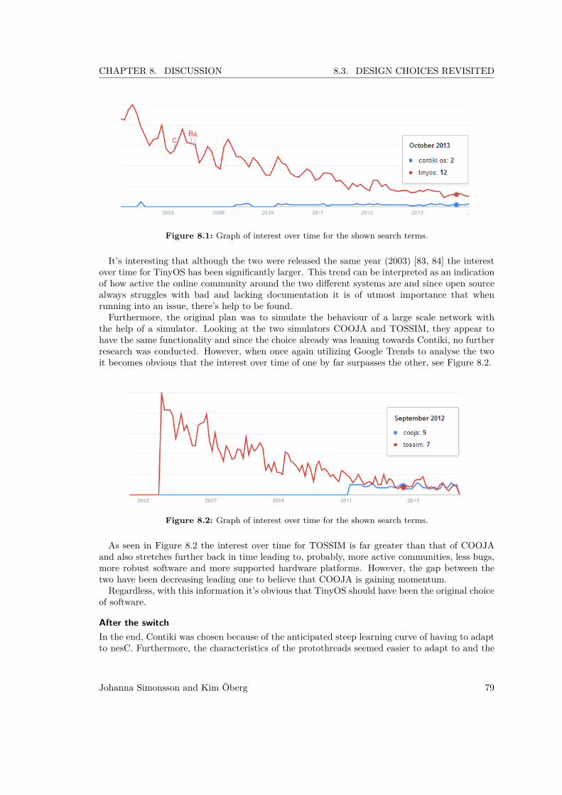
CHAPTER 8. DISCUSSION 8.3. DESIGN CHOICES REVISITED
Figure 8.1: Graph of interest over time for the shown search terms.
It’s interesting that although the two were released the same year (2003) [83, 84] the interestover time for TinyOS has been significantly larger. This trend can be interpreted as an indicationof how active the online community around the two different systems are and since open sourcealways struggles with bad and lacking documentation it is of utmost importance that whenrunning into an issue, there’s help to be found.Furthermore, the original plan was to simulate the behaviour of a large scale network with
the help of a simulator. Looking at the two simulators COOJA and TOSSIM, they appear tohave the same functionality and since the choice already was leaning towards Contiki, no furtherresearch was conducted. However, when once again utilizing Google Trends to analyse the twoit becomes obvious that the interest over time of one by far surpasses the other, see Figure 8.2.
Figure 8.2: Graph of interest over time for the shown search terms.
As seen in Figure 8.2 the interest over time for TOSSIM is far greater than that of COOJAand also stretches further back in time leading to, probably, more active communities, less bugs,more robust software and more supported hardware platforms. However, the gap between thetwo have been decreasing leading one to believe that COOJA is gaining momentum.Regardless, with this information it’s obvious that TinyOS should have been the original choice
of software.
After the switchIn the end, Contiki was chosen because of the anticipated steep learning curve of having to adaptto nesC. Furthermore, the characteristics of the protothreads seemed easier to adapt to and the
Johanna Simonsson and Kim Öberg 79

CHAPTER 8. DISCUSSION 8.3. DESIGN CHOICES REVISITED
feature of programming and building applications in a Virtualbox installation of Instant Contikiseemed straight forward. Expertise regarding Contiki was also available at the company, and theOS was used in a previous related project.
However, after having learned that Contiki suffered from issues which were difficult, if notimpossible, to overcome without a well-documented source, it was decided to switch to TOSSIM.This solved the, at the time, critical issue of not being able to utilize the serial port in parallelwith the IPv6 radio. Learning nesC also proved to be less of an issue than expected thanks to awell documented and thought through API.
However, TOSSIM turned out to be more of a disappointment than COOJA since it has nographical user interface and only support MicaZ motes, at which point the simulation aspect ofthe thesis was down prioritized.
8.3.2 The hardware choice revisited
When the lacking hardware support was revealed it led to the notion that the hardware choicealso should have been more extensively researched. But again, the scope was considered too largealready and the initial online research didn’t reveal enough to change the decision. However, outof the 31 Contiki compatible platforms it would’ve been worth to at least research some of themore popular ones. Which those were was in retrospect determined with Google Trends, seeFigure 8.3.
Figure 8.3: Graph of interest over time for the shown search terms.
As can be seen in Figure 8.3 the TelosB/Tmote Sky platform has a longer history of activ-ity/interest online but it has been declining over time. The predecessor of the IRIS mote, theMicaZ, was also very popular a few years ago (IRIS is too new to generate enough traffic to showup in Google Trends). Looking at this information it’s obvious why the software has the mostsupport for TMote Sky/TelosB and MicaZ (COOJA and TOSSIM respectively), they’ve beenaround the longest and are by far the most popular. Had this been known, the hardware choicewould’ve most definitely been different.
To further compare them a table was put together, see Table I below, in which it’s apparentthat they differ very little in actual hardware why the research related to popularity and interestover time becomes even more important.
80 Johanna Simonsson and Kim Öberg

CHAPTER 8. DISCUSSION 8.3. DESIGN CHOICES REVISITED
Table I: Characteristics of the TMote Sky, IRIS and Z1 motes [27, 28, 29].Evaluation criteria TMote Sky/TelosB Crossbow IRIS Zolertia Z1ProcessorMCU TI MSP430F1611 Atmel ATmega1281 TI MSP430F2617VCC 1.8 ... 3.6 V 2.7 ... 3.6 V 2.1 ... 3.6 VFlash 48 kB 128 kB 92 kBRAM 10 kB 8 kB 8 kBADC 12 bit 10 bit 12 bitCurrent draw: Active 0.5 mA @ 1MHz 8 mA @ 4MHz 0.5 mA @ 1MHzCurrent draw: Sleep 2.6 uA 8 uA 0.5 uA
RF TransceiverRadio chip TI CC2420 Atmel RF230 TI CC2420Data rate 250 kbps 250 kbps 250 kbpsTransmission power 0 : –25 dBm 0 : –24 dBm 0 : –25 dBmTX range outdoors (0 dB) 125 m > 300 m 180 m (antenna)Current draw: RX 19.7 mA 16 mA 18.8 mACurrent draw: TX 17.4 mA @ 0dBm 17 mA @ 3dBm 17.4 mA @ 0dBmCurrent draw: Sleep 1 uA 1 uA < 1 uA
ElectromechanicalGPIO 16 pin 51 pin expansion 52 pinOnboard sensors 3 - 3Power supply AA/USB AA/USB AA/micro USBUser interface 1 button, 3 LEDs 3 LEDs 1 button, 3 LEDsCost € 77 € 95
8.3.3 Simulators
As mentioned in Section 8.3.2 COOJA didn’t support the chosen hardware in the way, or to theextent, that was expected. On Contiki’s homepage no differentiation is made between the differentsupported hardware platforms leading one to believe that a further investigation is unnecessary.That however, proved not to be the case.
Almost all code examples in COOJA support the TMote Sky motes but few support the ZolertiaZ1. Furthermore, the function ’collect view’, which allows real time tracking of battery power,packet loss, packet latency, temperature sensor value and so forth, turned out to only supportthe TMote Sky. This played a part in the switch to the TinyOS system as it was believed, aftersome initial research, to be more robust, extensive and that the TOSSIM simulator supportedmore platforms.
That however, was not the case. In fact, TOSSIM only supports the MicaZ motes when simu-lating on hardware. Leading the switch to TinyOS to be virtually useless in terms of simulatorabilities.
However, when once again utilizing Google Trends to analyse a number of open source networksimulators it becomes obvious that perhaps a completely different choice of simulator should havebeen made, see Figure 8.4.
Johanna Simonsson and Kim Öberg 81

CHAPTER 8. DISCUSSION 8.3. DESIGN CHOICES REVISITED
Figure 8.4: Graph of interest over time for the shown search terms.
As seen in Figure 8.4 the interest over time for OMNeT++ and ns-3 is far greater than thatof COOJA/TOSSIM and also stretches further back in time leading to, probably, more activecommunities, less bugs, more robust software and more supported hardware platforms. However,the original scope didn’t leave much room for learning a completely new simulator program,instead the aim was to use COOJA/TOSSIM to simply verify that the actual written code couldscale as the great benefit of those simulators are that one can compile actual source code andsimulate it on nodes in the program. And had only the hardware been different many issuescould’ve been avoided.
8.3.4 Back endThe back end of the system consists of the MVC Django which is written in Python. No actualresearch was conducted into the area of MVCs as Python was a known language and the proposedoptions in PHP and Ruby would’ve required learning a new language. However, looking back,very few of the Django’s functionalities are actually utilized leading to the conclusion that maybeanother MVC could’ve done the job better? An initial online survey of internet forums revealedCodeIgniter (PHP) and Ruby on Rails (Ruby) as the biggest contenders. Again, Google Trendswas used to analyse the interest over time for the different frameworks, see Figure 8.5.
Figure 8.5: Interest over time for Django (Python), CodeIgniter (PHP) and Ruby on Rails (Ruby).
The graph in Figure 8.5 clearly shows that, at least historically, Ruby on Rails had the mostactive online community and highest interest. But lately PHP based CodeIgniter and Djangohave been gaining momentum leading to the conclusion that the choice of Django probably didn’tinfluence the thesis in a negative way. Rather, time was saved by choosing an already familiarlanguage (Python).
82 Johanna Simonsson and Kim Öberg

CHAPTER 8. DISCUSSION 8.4. THE HYPOTHESES REVISITED
8.4 The hypotheses revisitedAs outlined in Section 1.3 (Hypothesis) a couple of hypotheses were developed during the back-ground study to be used as guidelines during the master thesis. This section will briefly summarizethe findings related to each hypothesis as well as make references to the relevant paragraphs inthe thesis.
• A suitable setup for an irrigation system consists of sensor nodes, soil moisture sensors,one sink node and a main frame functioning as back-end.
Yes, as presented in Section 2.2 (Characteristics of WSN ) and 3.2 (WSN in precision agri-culture) most existing WSN deployment aimed at irrigation utilize soil moisture sensors,some kind of grid pattern for the sensor nodes, one (or more depending on size) sink nodesand a back-end of some sort.
• Weather data can be used to lower power consumption.
Yes. As shown in Section 6.2 (Dynamic sleep intervals) utilizing weather to determine sleepintervals could indeed lower the power consumption of the network.
• A feedback system could improve the performance of the system.
As no actual deployment was carried out there is no way of definitely knowing whether theproposed feedback solution will indeed improve the performance. However, as discussed inSection 4.2 (System control loop) and 6.2 (Dynamic sleep intervals).
• The routing scheme can be self-healing and robust without drawing too much power.
Yes and no. There is no easy answer to this question as shown in Section 3.3.3 (Robustness),6.1 (Network design) and 6.1.1 (TinyRPL vs MOECS) since each installation, dependingon use, size and purpose will have to weigh the pros and cons of a, somewhat, energy costlyrobust network against the pros and cons of a less power consuming and less robust sys-tem. But the results in 6.1.1 (TinyRPL vs MOECS) are promising when it comes to powerconsumption of a self-healing and self-organizing robust network.
• The most important design decisions related to power management are power mode han-dling and network setup.
Yes and no. It’s been discussed in both Section 3.3.2 and 3.3.6 that these two are pivotalwhen managing the power dissipation of the system but what can be an even bigger culpritis the sensors, as discussed in Section 6.2 and 8.1.1.
After revisiting the hypotheses, the conclusion is that a lot of knowledge has been gained onhow to design a WSN-based smart irrigation system. However, as mentioned in 1.4 (Scope),what’s also become evident is how much more knowledge, outside of the embedded softwaredomain, that is needed for a successful deployment.The challenge lies in designing a well-functioning routing protocol while keeping energy cost
from peripheral components, like the sensor, down to a minimum. There are still some work to bedone before the prototype can be tested in a real-life deployment and those possible improvementsare presented in Chapter 9.
Johanna Simonsson and Kim Öberg 83

9 Future workIn this chapter the future work related to the discussed topics in Section 6 (Analysis) and 8(Discussion) will be presented.
9.1 HardwareIn this section the different future solutions for hardware will be presented. All recommendationsfor future work are based on the discussions in Section 8.1.2 and 8.3.2.
9.1.1 NodesAs mentioned in 8.3.2 the original choice of the Zolertia Z1 node proved to be less than ideal. Thiswas mainly due to the issues mentioned in 8.1.3, namely that the RAM memory was too small forthe TinyRPL-programs but also that the hardware not being supported fully by the simulators.Furthermore, the analysis in 8.3.2 clearly shows how other hardware platforms outperform theZolertia Z1 in terms of interest over time and thereby active online community.As a result, the future work regarding hardware would be to switch to the TelosB/Tmote Sky
platform, since it’s fully compatible with the software and simulators, have more RAM storageand a larger online community.
9.1.2 SensorsThe switch to the TelosB/Tmote Sky platform does however not solve the issue with the soilmoisture sensor mentioned in Section 8.1.2. It still needs a voltage supply of 3.3V or 5V to runproperly, which requires an external battery powered circuit solely for the sensor or that theentire sensor be replaced.The future work here consists of finding a better suited sensor (which can run on 3V) or to
construct an external circuit.The other problem mentioned in Section 8.1.1 were the use of a sampling interval that was
estimated according to different sources. Work conducted to finding an optimal sampling intervalwould therefore improve the system, and is also suggested as future work.As the availability of sensors online were limited, another approach and future work would be
to develop a soil moisture sensor with low power consumption suitable for the application.
9.2 SoftwareIn this section the different future solutions for software will be presented. All recommendationsfor future work are based on the discussions in Section 8.1.3 and 8.3.1.
9.2.1 Operating system on nodesAs mentioned in both 4.3.1 and 8.3.1 the issues with the chosen software are tightly linked to thechosen hardware. If the hardware is disregarded there have been no major issues with neitherContiki nor TinyOS, besides the bug in Contiki which made it impossible to utilize the serialport while simultaneously listening to radio messages.Furthermore, the initial analysis regarding routing protocols suggest that a IPv6 compliant
84

CHAPTER 9. FUTURE WORK 9.2. SOFTWARE
routing protocol would outperform RPL. Therefore an implementation of an IPV6 compliantcluster-based routing protocol would be a preferable future work.On the same note, the data aggregation algorithm is still not very refined in this thesis can
could definitely be improved for better performance over all.
9.2.2 Simulator softwareAnother quite necessary aspect of the future work concerns the simulators. Both COOJA andTOSSIM, with the right hardware, could probably deliver satisfactory results if enough time weregiven. However, OMNET++ is regarded as one of the best network simulators and probablytherefore a good choice for evaluating routing metrics. So, in short, the future work consists of:
• If TinyOS: Keep the serial approach but if IPv6 is the goal then there’s no point in utilizingthe serial port, then everything should go via a web server.
• Implement a IPv6 compliant cluster based routing protocol.• Utilize a proper network simulator to verify initial results regarding routing.
9.2.3 Back-endAs mentioned in the Method section 4.4.1, the chosen database implementation SQLite haveshortcomings not suitable for a bigger deployment than the one conducted in this project. Thechoice were mainly made on the fact that neither of the project participants had any previousknowledge on how to handle and implement databases. SQLite have the advantage of beingeasy to setup and therefore a good alternative for inexperienced users. To ensure scalability andfeatures like users and permission management, future work would be to implement a bettersuited database. After a quick screening by utilizing the Google Trends tool and consulting withthe company, a good choice of replacement for SQLite would probably be MySQL, see Figure9.1.
Figure 9.1: Graph of interest over time for the shown search terms.
9.2.4 Front-endAs mentioned in Section 1.4 (Scope), implementing any kind of user interface was outside thescope, as it wasn’t needed to perform the task. However, the advantage with having a front-endsystem is the possibility to easy evaluate the data that is stored which could improve the over-allperformance. Therefore a possible future work would be to develop some kind of front-end systemwith the possibility to analyse the stored data.
Johanna Simonsson and Kim Öberg 85
CHAPTER 9. FUTURE WORK 9.3. IMPLEMENTATION OF PHYSICAL TEST-BED
9.3 Implementation of physical test-bedAs been mentioned throughout the whole project, as the field of study being Mechatronics, areal-life implementation have not been possible. However, if the discussed design choices shouldbe tested thoroughly, they need to be tested in a real life deployment. This would mean acollaboration together with ethnographers, biologist, irrigation hardware specialists etc. Many ofthe difficulties with handling electronic solutions in agriculture are directly dependent on the factthat the environment is hostile. Many of the assumptions and design choices might be invalid ifknowledge for the actual deployment environment is disregarded.If a real-life deployment were to be implemented, it would probably result in a similar setup
as in [6, 7, 5, 9, 55], with a deployment of approximately the same amount of nodes as in thetest-bed chosen in Section 6.1. However, a lot of work to be conducted before this set-up couldbe possible, even after the issues brought up in Section 8.1 have been cleared.Some of the benefits of doing this kind of deployment are mentioned in the bullet list below:
• Evaluate if sensors other than the soil moisture one should benefit the system.
• Finding out what kind of features the nodes need to ensure robustness outside.
• The actual battery life of the nodes could be studied.
• Study the actual packet-loss that are due to outer factors.
9.4 VerificationAs mentioned in Section 8.1.1, the technique used to estimate the battery life span was notaccurate enough. Future work would here be to build a current measuring setup good enough toaccurately measure the small currents on the sensor nodes, along with a simulation environmentto test the results [104].
86 Johanna Simonsson and Kim Öberg

10 ConclusionThe system design choices of a smart networked irrigation system is a balancing act between theavailable energy of the network sensors and the acceptable maximum packet loss ratio (robust-ness). To be able to achieve a satisfying end-product, adapting the choices to the implementationis of utmost importance. The design choices discussed and evaluated in this master thesis include:
• Hardware choices: Choosing hardware with a low power consumption is essential if thesystem is going to have a long life span. Deciding on a power-efficient and reliable sensor isespecially important as the sensor is the component which consumes the most energy. 8.3
• Network: How the network is designed is one of the most important design decisions,and includes several sub-categories including; network topology, routing protocol, dataaggregation scheme and so on. Choosing an appropriate network will greatly affect howwell the system is performing. 6.1
To take advantage of both sensors and online weather data services, a feedback control loopis proposed to gain precision on water dispersed, and with that increasing crop yield and savingwater. With this proposed feedback-loop a solution to dynamically change the sleep interval isintroduced. By changing how long the sensor nodes are turned off in proportion to how muchprecipitation is expected, the nodes can save up to 30 +% of the available energy . Furthermorean improved solution, also proposed in this master thesis, is to dynamically change the sleepintervals according to how ET fluctuates over the course of 24 hours or perhaps a week, insteadof keeping ET static for long periods of time. 6.2Smart irrigation systems are meant to be deployed in agricultural contexts, and every area of
deployment have unique characteristics which can differ greatly from each other. Therefore it isimportant to take the unique on-site variations into consideration while designing the system toacquire the optimal performance of said system. To further analyze the results acquired in thisthesis, a real-life deployment analysing network behaviour and life span would greatly increasethe understanding of said system. The knowledge gained could be used to improved the systemeven further. 9
87

Bibliography[1] A.A. Ahmed, Hongchi Shi, and Yi Shang. A survey on network protocols for wireless
sensor networks. In Information Technology: Research and Education, 2003. Proceedings.ITRE2003. International Conference on, pages 301–305, Aug 2003.
[2] Luis Ruiz-Garcia, Loredana Lunadei, Pilar Barreiro, and Ignacio Robla. A review of wirelesssensor technologies and applications in agriculture and food industry: State of the art andcurrent trends. Sensors, 9(6):4728–4750, 2009. ISSN 1424-8220. URL http://www.mdpi.com/1424-8220/9/6/4728.
[3] Hervé Guyennet Mourad Hadjila and Mohammed Feham. A chain-based routing protocolto maximize the lifetime of wireless sensor networks. Wireless Sensor Network, 5(5):p. 116,2013. ISSN 19453078.
[4] U.S. Department of the Interior Bureau of Reclamation. Weather- and soil moisture-basedlandscape irrigation scheduling devices. Technical Review Report 4, U.S. Department ofthe Interior Bureau of Reclamation, Lower Colorado Region, July 2012.
[5] J. Burrell, T. Brooke, and R. Beckwith. Vineyard computing: sensor networks in agricul-tural production. Pervasive Computing, IEEE, 3(1):38–45, Jan 2004. ISSN 1536-1268.
[6] Aleksandar Kovacevic Janne Riihijarvi Christine Jardak, Krisakorn Rerkrai and Petri Ma-honen. Design of large-scale agricultural wireless sensor networks: email from the vineyard.International Journal of Sensor Networks, 8(2):77–88, Jan 2010. ISSN 1536-1268.
[7] R. Beckwith, D. Teibel, and P. Bowen. Unwired wine: sensor networks in vineyards. InSensors, 2004. Proceedings of IEEE, pages 561–564 vol.2, Oct 2004.
[8] Keith Bellingham. Method for irrigation scheduling based on soil moisture data acquisition.United States Committee on Irrigation and Drainage, 2009.
[9] Langendoen K., Baggio A., and Visser O. Murphy loves potatoes: experiences from a pilotsensor network deployment in precision agriculture. In Parallel and Distributed ProcessingSymposium, 2006. IPDPS 2006. 20th International, pages 8 pp.–, April 2006. doi: 10.1109/IPDPS.2006.1639412.
[10] J.B. Patel, C.B. Bhatt, B. Patel, K. Parwani, and C. Sohaliya. Field irrigation managementsystem using wireless sensor network. In Engineering (NUiCONE), 2011 Nirma UniversityInternational Conference on, pages 1–4, Dec 2011.
[11] Torkel Glad and Lennart Ljung. Reglerteknik: Grundläggande teori. Studentlitteratur,2006. ISBN 9789144022758.
[12] Lloyed Sealy Library. What is a peer-reviewed article? URL http://guides.lib.jjay.cuny.edu/content.php?pid=209679&sid=1746812. Accessed: 2014-02-27.
[13] Richard G. Allen. Crop evapotranspiration: guidelines for computing crop water require-ments. FAO, Rome, 1998. ISBN 92-5-104219-5.
88
Bibliography Bibliography
[14] Allan A Andales, JL Chávez, and Troy Allen Bauder. Irrigation Scheduling: The Water-balance Approach, volume 4. Colorado State University Extension, 2011.
[15] George H. Hargreaves and Gary P. Merkley. Irrigation Fundamentals: An Applied Technol-ogy Text for Teaching Irrigation at the Intermediate Level. Water Resources Pubns, 1998.ISBN 978-1887201100.
[16] Zahariah Manap, BorhanuddinMohd Ali, CheeKyun Ng, NorKamariah Noordin, andAduwati Sali. A review on hierarchical routing protocols for wireless sensor networks.Wireless Personal Communications, 72(2):1077–1104, 2013. ISSN 0929-6212. URL http://dx.doi.org/10.1007/s11277-013-1056-5.
[17] Hervé Guyennet Mourad Hadjila and Mohammed Feham. A chain-based routing protocolto maximize the lifetime of wireless sensor networks. Wireless Sensor Network, 5:116, 2013.
[18] Kemal Akkaya and Mohamed Younis. A survey on routing protocols for wireless sensornetworks. Ad Hoc Networks, 3(3):325 – 349, 2005. ISSN 1570-8705. URL http://www.sciencedirect.com/science/article/pii/S1570870503000738.
[19] Network Design Basics for Cabling Professionals. Bicsi Press Series. Mcgraw-hill, 2002.ISBN 9780071399166. URL http://books.google.se/books?id=uRKq-g6z6fYC.
[20] Kevin P. Scheibe and Cliff T. Ragsdale. A model for the capacitated, hop-constrained, per-packet wireless mesh network design problem. European Journal of Operational Research,197(2):773 – 784, 2009. URL http://www.sciencedirect.com/science/article/pii/S0377221708005626.
[21] Yanping Xiang and Gregory Levitin. Service task partition and distribution in star topol-ogy computer grid subject to data security constraints. Reliability Engineering and Sys-tem Safety, 96(11):1507 – 1514, 2011. URL http://www.sciencedirect.com/science/article/pii/S0951832011001323.
[22] C. Delestre, G. Ndo, and F. Labeau. A binary tree network topology for statistical andphysical plc channel modeling. Power Line Communications and Its Applications (ISPLC),2013 17th IEEE International Symposium on, pages 327–332, mar 2013.
[23] Bo Chang and Xinrong Zhang. An energy-efficient cluster-based data gathering protocol forwireless sensor networks. In Wireless Communications Networking and Mobile Computing(WiCOM), 2010 6th International Conference on, pages 1–5, Sept 2010. doi: 10.1109/WICOM.2010.5601147.
[24] Bo Peng Ana Maria Popescu, Ion Gabriel Tudorache and A. H. Kemp. Surveying positionbased routing protocols for wireless sensor and ad-hoc networks. International Journalof Communication Networks and Information Security (IJCNIS), Vol.4(1):p.41(27), April2012. ISSN 2076-0930.
[25] Yongchang Yu and Yichang Song. An energy-efficient chain-based routing protocol inwireless sensor network. In Computer Application and System Modeling (ICCASM), 2010International Conference on, volume 11, pages V11–486–V11–489, Oct 2010.
[26] W.B. Heinzelman, A.P. Chandrakasan, and H. Balakrishnan. An application-specific proto-col architecture for wireless microsensor networks. Wireless Communications, IEEE Trans-actions on, 1(4):660–670, Oct 2002. ISSN 1536-1276.
Johanna Simonsson and Kim Öberg 89

Bibliography Bibliography
[27] Zolertia. Z1 Datasheet, March 2010. URL http://zolertia.sourceforge.net/wiki/images/e/e8/Z1_RevC_Datasheet.pdf.
[28] Moteiv. TMote Sky Datasheet, 2006. URL http://www.eecs.harvard.edu/~konrad/projects/shimmer/references/tmote-sky-datasheet.pdf.
[29] Crossbow. IRIS Datasheet. URL http://www.memsic.com/userfiles/files/Datasheets/WSN/IRIS_Datasheet.pdf.
[30] Alextronix Controls. Alextronix controller. URL http://www.alextronix.com/enercon4-24plus.htm. Accessed: 2014-04-29.
[31] Irritrol Systems. Irritrol controllers, . URL http://www.irritrolsystems.com/controllers/controllers.html. Accessed: 2014-04-29.
[32] Rain Drip. Rain drip timers. URL http://www.raindrip.com/timers. Accessed: 2014-04-29.
[33] Rain Bird. Rain bird controllers. URL http://www.rainbird.com/landscape/products/controllers/index.htm. Accessed: 2014-04-29.
[34] Accurate WeatherSet. Accurate weatherset homepage. URL http://weatherset.com/.Accessed: 2014-04-29.
[35] Hydrosaver. Hydrosaver controllers. URL http://www.hydrosaver.net/Items.aspx?catId=c01. Accessed: 2014-05-02.
[36] Hunter Industries. Hunter controllers. URL http://www.hunterindustries.com/product-line/controllers. Accessed: 2014-04-29.
[37] Calsense. Calsense controllers. URL http://www.calsense.com/controllers/. Accessed:2014-04-29.
[38] WeatherMatic. Smartline. URL http://www.weathermatic.com/content/smartline.Accessed: 2014-04-29.
[39] ETWater. Etwater solutions. URL http://www.etwater.com/solutions-products. Ac-cessed: 2014-04-29.
[40] Inc Tucor. Tucor, inc. URL http://www.tucor.com/index-2.html. Accessed: 2014-04-29.
[41] Irrisoft. Irrisoft. URL http://www.irrisoft.net/products.htm. Accessed: 2014-04-29.
[42] Inc. HydroPoint Data Systems. Outdoor solutions overview. URL http://www.hydropoint.com/products/outdoor-solutions/. Accessed: 2014-04-29.
[43] Weather Reach. Weather reach signal stations map. URL http://www.weatherreach.com/index.php/weather-reach-signal-service.html. Accessed: 2014-05-01.
[44] Rain Master Control Systems. Rain master main page, . URL http://www.rainmaster.com/. Accessed: 2014-05-01.
[45] Cyber Rain. Smart irrigation controller product overview. URL https://www.cyber-rain.com/smart-irrigation-controller-product-overview.html. Accessed:2014-05-01.
90 Johanna Simonsson and Kim Öberg

Bibliography Bibliography
[46] MorpH20. Aguamiser. URL http://www.morph2o.com/turf-landscape/aguamiser/.Accessed: 2014-05-02.
[47] Acclima. Acclima products. URL http://acclima.com/wd/index.php?option=com_content&view=article&id=7&Itemid=2. Accessed: 2014-04-29.
[48] Dynamax. Soil moisture. URL http://www.dynamax.com/IrrigationControl.htm. Ac-cessed: 2014-04-29.
[49] Baseline Systems. Baseline products, . URL http://www.baselinesystems.com/products.php. Accessed: 2014-04-29.
[50] Wikipedia. Precision agriculture, . URL http://en.wikipedia.org/wiki/Precision_agriculture. Accessed: 2014-06-02.
[51] Memsic. eKo Outdoor Wireless System. URL http://www.memsic.com/userfiles/files/Datasheets/WSN/eko_starter_system.pdf. Accessed: 2014-05-14.
[52] Inc. Spectrum Technologies. WatchDog Wireless Crop Monitors PRODUCT MANUAL.URL http://www.specmeters.com/assets/1/22/3540.pdf. Accessed: 2014-05-14.
[53] Inc. Netafim Irrigation. Irriwise wireless radio crop monitoring. URL http://www.netafimusa.com/agriculture/products/wireless-radio-crop-monitoring. Ac-cessed: 2014-05-14.
[54] Xiong Shu-ming, Wang Liang-Min, Qu Xiao-qian, and Zhan Yong-Zhao. Application re-search of wsn in precise agriculture irrigation. In Environmental Science and InformationApplication Technology, 2009. ESIAT 2009. International Conference on, volume 2, pages297–300, July 2009. doi: 10.1109/ESIAT.2009.231.
[55] Balendonck J., Hemming, J. Tuijl, B.A.J. van Incrocci, L. Pardossi, and A. Marzialetti P.Sensors and wireless sensor networks for irrigation management under deficit conditions(flow-aid). In Conference Proceedings CD of the International Conference on AgriculturalEngineering / Agricultural and Biosystems Engineering for a Sustainable World. - EurA-gEng (European Society of Agricultural Engineers), Wageningen UR Glastuinbouw, 2008.
[56] Ding J.-W. Wang, C.-F. and Lee. Joint optimization of energy allocation and routingproblems in wireless sensor networks. Wireless Communications and Mobile Computing,10(2):171–178, 2010.
[57] H. Balakrishnan W. Heinzelman, A. Chandrakasan. Energy efficient communication pro-tocol for wireless microsensor networks. In Proceedings of the 33rd Annual Hawaii Inter-national Conference on System Sciences, volume 1, 2000.
[58] Guihai Chen Mao Ye, Chengfa Li and Jie Wu. Eecs: an energy efficient clustering schemein wireless sensor networks. In Performance, Computing, and Communications Conference,2005. IPCCC 2005. 24th IEEE International, pages 535–540, April 2005.
[59] Nauman Aslam, William Phillips, William Robertson, and Shyamala Sivakumar. A multi-criterion optimization technique for energy efficient cluster formation in wireless sensornetworks. Information Fusion, 12(3):202 – 212, 2011. ISSN 1566-2535. URL http://www.sciencedirect.com/science/article/pii/S1566253509000992. Special Issue onInformation Fusion in Future Generation Communication Environments.
Johanna Simonsson and Kim Öberg 91

Bibliography Bibliography
[60] Jin Wang, Yu Niu, Jinsung Cho, and Sungyoung Lee. Analysis of energy consumptionin direct transmission and multi-hop transmission for wireless sensor networks. In Signal-Image Technologies and Internet-Based System, 2007. SITIS ’07. Third International IEEEConference on, pages 275–280, Dec 2007. doi: 10.1109/SITIS.2007.145.
[61] Holger Karl and Andreas Willig. Protocols and Architectures for Wireless Sensor Networks.John Wiley and Sons Ltd, Chichester, UK, 2006. ISBN 0-470-09510-5.
[62] W. Robertson W.J. Phillips F. Comeau, S.C. Sivakumar. Energy conserving architecturesand algorithms for wireless sensor networks. In Proceedings of the 39th Annual HawaiiInternational Conference on System Sciences, volume 09, 2006.
[63] H. Balakrishnan W. Heinzelman, A. Chandrakasan. Ieee transactions on wireless commu-nications. In Proceedings of the 39th Annual Hawaii International Conference on SystemSciences, volume 1, page 660–670, 2002.
[64] TIK WSN Research Group. Sensor network hardware systems, 2014. URL http://www.snm.ethz.ch/.
[65] Susanne Albers. Energy-efficient algorithms. Commun. ACM, 53(5):86–96, May 2010. ISSN0001-0782. URL http://doi.acm.org/10.1145/1735223.1735245.
[66] J. Augustine, S. Irani, and C. Swamy. Optimal power-down strategies. In Foundations ofComputer Science, 2004. Proceedings. 45th Annual IEEE Symposium on, pages 530–539,Oct 2004.
[67] Texas Instruments. MIXED SIGNAL MICROCONTROLLER MSP430F261x, 2012. URLhttp://www.ti.com/lit/ds/symlink/msp430f2617.pdf.
[68] Waltenegus Dargie. Dynamic power management in wireless sensor networks: State-of-the-art. Sensors Journal, IEEE, 12(5):1518–1528, May 2012.
[69] A. Sinha and A. Chandrakasan. Dynamic power management in wireless sensor networks.Design Test of Computers, IEEE, 18(2):62–74, Mar 2001. ISSN 0740-7475.
[70] F. Yao, A. Demers, and S. Shenker. A scheduling model for reduced cpu energy. InFoundations of Computer Science, 1995. Proceedings., 36th Annual Symposium on, pages374–382, Oct 1995.
[71] Isam Ishaq, David Carels, Girum K. Teklemariam, Jeroen Hoebeke, Floris Van den Abeele,Eli De Poorter, Ingrid Moerman, and Piet Demeester. Ietf standardization in the field ofthe internet of things (iot): A survey. Journal of Sensor and Actuator Networks, 2(2):235–287, 2013. ISSN 2224-2708. doi: 10.3390/jsan2020235. URL http://www.mdpi.com/2224-2708/2/2/235.
[72] Escotal.Com. Osi 7 layer model, 2013. URL http://www.escotal.com/osilayer.html.Accessed: 2014-05-15.
[73] R. Braden. Requirements for internet hosts - communication layers. RFC Editor, 1989.
[74] V. Cerf, Y. Dalal, and C. Sunshine. Specification of internet transmission control program.IETF, (675), December 1974. URL http://www.ietf.org/rfc/rfc675.txt.
[75] J. Postel. User datagram protocol. 1980.
92 Johanna Simonsson and Kim Öberg

Bibliography Bibliography
[76] Wikipedia. The internet protocol, . URL http://en.wikipedia.org/wiki/Internet_Protocol. Accessed: 2014-05-20.
[77] J.W. Hui and D.E. Culler. Extending ip to low-power, wireless personal area networks.Internet Computing, IEEE, 12(4):37–45, July 2008. ISSN 1089-7801. doi: 10.1109/MIC.2008.79.
[78] Olfa Gaddour and Anis Koubâa. {RPL} in a nutshell: A survey. Computer Networks, 56(14):3163 – 3178, 2012. ISSN 1389-1286. doi: http://dx.doi.org/10.1016/j.comnet.2012.06.016. URL http://www.sciencedirect.com/science/article/pii/S1389128612002423.
[79] Texas Instruments. IPv6 over Low-Power Wireless Personal Area Networks (6LoWPANs):Overview, Assumptions, Problem Statement, and Goals, 2007. URL http://tools.ietf.org/html/rfc4919.
[80] Texas Instruments. Problem Statement and Requirements for IPv6 over Low-Power Wire-less Personal Area Network (6LoWPAN) Routing, 2012. URL http://tools.ietf.org/html/rfc6606.
[81] Wikipedia. Contiki, . URL http://en.wikipedia.org/wiki/Contiki. Accessed: 2014-05-05.
[82] Wikipedia. Tinyos, . URL http://en.wikipedia.org/wiki/TinyOS. Accessed: 2014-05-05.
[83] Björn Grönvall Adam Dunkels and Thiemo Voigt. Contiki - a lightweight and flexible oper-ating system for tiny networked sensors. Technical report, Swedish Institute of ComputerScience, 2004.
[84] TinyOS. The tinyos homepage, . URL http://www.tinyos.net/. Accessed: 2014-05-09.
[85] Joakim Eriksson Niclas Finne Fredrik Österlind, Adam Dunkels and Thiemo Voigt. Cross-level sensor network simulation with cooja. Technical report, Swedish Institute of ComputerScience, 2006.
[86] TinyOS. Tinyrpl, oct 2011. URL http://tinyos.stanford.edu/tinyos-wiki/index.php/TinyRPL. Accessed: 2014-06-03.
[87] TinyOS. Mote-mote radio communication, . URL http://tinyos.stanford.edu/tinyos-wiki/index.php/Mote-mote_radio_communication. Accessed: 2014-06-03.
[88] Texas Instruments. MSP430 Ultra-Low-Power Microcontrollers, 2014. URL http://ti.com/msp430.
[89] Brent Q. Mecham. A practical guide to using soil moisture sensors to control landscapeirrigation. Northern Colorado Water Conservancy District, Loveland, Colorado, 2010.
[90] Lawrence J. Schwankl. Electrical resistance blocks. Technical report, Division of Agricultureand Natural Resources, University of California, 2014.
[91] Darold Wobschall and Deepak Lakshmanan. Wireless soil moisture sensor based on fringingcapacitance.
[92] Vegetronix. Vh400 soil moisture sensor probes. URL http://www.vegetronix.com/Products/VH400/. Accessed: 2014-05-27.
Johanna Simonsson and Kim Öberg 93
Bibliography Bibliography
[93] Irrometer. Model 200ss watermark sensor. URL http://www.irrometer.com/pdf/sensors/403%20Sensor%20%20Web5.pdf. Accessed: 2014-05-27.
[94] DF Robot. Soil moisture sensor. URL http://www.dfrobot.com/index.php?route=product/product&product_id=599#.U4R9CdJ_vy0. Accessed: 2014-05-27.
[95] Django Software Foundation. Official django homepage. URL https://www.djangoproject.com/. Accessed: 2014-03-28.
[96] Hal Werner. Measuring soil moisture for irrigation water management. Computer Networks,2002.
[97] Xianghui Fan, Shining Li, Zhigang Li, and Jingyuan Li. Sensors Dynamic Energy Manage-ment in WSN. Wireless Sensor Network, 2010.
[98] SMHI. Nederbord. URL http://www.smhi.se/klimatdata/meteorologi/nederbord. Ac-cessed: 2014-05-29.
[99] C. Thimmannagari. CPU Design: Answers to Frequently Asked Questions. Springer, 2005.ISBN 9780387238005. URL http://books.google.se/books?id=_MBoceOixmoC.
[100] Hoang Anh Nguyen, A. Forster, D. Puccinelli, and S. Giordano. Sensor node lifetime: Anexperimental study. In Pervasive Computing and Communications Workshops (PERCOMWorkshops), 2011 IEEE International Conference on, pages 202–207, March 2011. doi:10.1109/PERCOMW.2011.5766869.
[101] BitBox. Results: Low drain, 2012. URL http://www.batteryshowdown.com/results-lo.html. Accessed: 2014-05-19.
[102] Texas Instruments. CC2420 2.4 GHz IEEE 802.15.4 / ZigBee-ready RF Transceiver, 2014.URL http://www.ti.com/lit/ds/symlink/cc2420.pdf.
[103] Energizer. Battery comparison. URL http://www.energizer.com/learning-center/Pages/battery-comparison.aspx. Accessed: 2014-06-03.
[104] Chulsung Park, K. Lahiri, and A. Raghunathan. Battery discharge characteristics of wire-less sensor nodes: an experimental analysis. In Sensor and Ad Hoc Communications andNetworks, 2005. IEEE SECON 2005. 2005 Second Annual IEEE Communications SocietyConference on, pages 430–440, Sept 2005. doi: 10.1109/SAHCN.2005.1557096.
[105] H.R. Kermajani and C. Gomez. Route change latency in low-power and lossy wirelessnetworks using rpl and 6lowpan neighbor discovery. In Computers and Communications(ISCC), 2011 IEEE Symposium on, pages 937–942, June 2011. doi: 10.1109/ISCC.2011.5983962.
[106] Google. Google trends. URL https://support.google.com/trends/answer/4355164?hl=en&rd=1. Accessed: 2014-05-09.
94 Johanna Simonsson and Kim Öberg
A Scope issues
Appendix to review the initial conditions of the project and the iterations made to reach thecurrent problem definition and scope.
A.1 Initial problem definitionInitially, the foundation for this project were created by Daniel Thysell at Sigma Technology. Hehad a vision for a project that focused on an engineering task which was summarized as:
• Mesh radio network for measuring moist level in plantation and combining that with onlineweather service to provide input to a pump system.
• Network to be controlled, managed and used by web-based user interface.• Classic Internet of Things-application.
However, as KTH expected a project which contained a scientific evaluation and the presentedone only contained an engineering task, the project were re-evaluated. Together with KTH andthe company the scope changed to focus on the power consumption aspect of the intended phys-ical system. The finalized problem definition were decided as:
”Can the over-all power consumption of the wireless sensor network be lowered with the help ofpower-efficient algorithms and network optimization based on the chosen implementation? Thechosen implementation being an autonomous irrigation system deployed over a large area (requiresa scalable system) with a significant amount of nodes, all connected to one central database. Thesystem output is a water distribution system (i.e a pump), and the system input will be collectedfrom moisture sensors and a local online weather service.”
To answer the research question, the chosen methodology consisted of a few steps. Firstly, afterconducting a background study, the parameters which affect the total power consumption of thesystem were to be identified. These parameters were to become the foundation of the workinghypothesis for the rest of thesis. When these had been identified, the task were to evaluate how(and if) these parameters could be tweaked/manipulated in order to decrease the over-all powerconsumption. To achieve this, the project were intended to do two different engineering tasks.Firstly, a prototype would be built of the defined system, with two sensor (Z1) nodes commu-
nicating with a main computer frame through a border router. This means that the first methodused would be a controlled experimental environment, where the nodes, sensors and main com-puter frame will be included. Secondly, in order to verify the behaviour of the prototype, andensure scalability, the system would also be simulated with a significantly larger amount of nodesin the software Cooja. The use of a simulation environment were intended as a complement tothe limitations of a controlled experiment, and ensure that the network communication would betested thoroughly.The time frame were set at 20 weeks and were intended to follow the time planning presented
in Figure A.1.
1

APPENDIX A. SCOPE ISSUES A.1. INITIAL PROBLEM DEFINITION
Figure A.1: A detailed Gantt Chart containing the schedule of the entire project.
The intended plan corresponded well to the working pace, a thoroughly conducted backgroundstudy were made. However, half-way into the project, several problems started to emerge.
2 Johanna Simonsson and Kim Öberg
APPENDIX A. SCOPE ISSUES A.2. SCOPE CHANGE
Firstly, to power optimize the intended system, one needs to have knowledge in several areas.Apart from knowing how power optimization works for networks and on node level, extensiveknowledge of the implemented system has to be obtained. The realisation gained was that it wasprobably best to have a complete system to analyse, and not to analyse something that wasn’timplemented from the start. This meant that the anticipated workload were far more great thanpreviously assumed.Secondly, problems with the intended simulation environment emerged. The simulation soft-
ware COOJA did not support the used hardware in the ways presumed when the project started.This meant that the second part of the engineering task were not possible to implement, andwith that a major part of the testing, validation and verification fell short.Apart from these two problems, more difficulties arose when the understanding of what the
problem definition actually promised increased. For example, a lot of the power consumed by thenodes corresponds to the chosen network implementation. Therefore, implementing a well-chosenrouting protocol matching a suitable test-bed is the best approach to ensure power optimization.However, implementing a functioning power-optimized routing protocol is not an easy task, andwould require both a lot of time and knowledge of the hardware, software and algorithms thatthe participants of the project did not have.Also, a part of the project were to evaluate where the power savings corresponding improve-
ments on node level could be made. However, most of the State Of the Art knowledge of thiskind of power saving techniques are already implemented on the operating systems designed to beused on sensor nodes. This meant the improvements made would probably be neither noticeablenor implementable. Also, if an actual improvement were implemented on the system, one wouldhave to be able to validate the power consumption on the node by utilizing some kind of way tomeasure current. As the nodes current levels are very tiny in size (micro Ampere) an advancedsetup had to be used, and that would require knowledge, resources and time not available.All these problems were enabled due to assumptions made in the beginning of the project
without any real knowledge backing the assumptions up. The problem definition promised farmore than was realistic for two mechatronic students to conduct during a 20 week period. Inshort, the scope was way too big.
A.2 Scope changeWhen the problems that had arisen in Section A.1 were analysed, the conclusion reached wasthat the scope was way too big. The only way to finish the master thesis within the time frameof 20 weeks was to reformulate the research question and with that the scope. The goal was tomake sure that the work conducted so far in this process hadn’t all been in vain. However, toreach many of the conclusions made in Section A.1, an extensive research had been conductedto the few relevant subjects. A gap in the market were discovered along the way, together withthe motivation on why an autonomous WSN based irrigation system was interesting in the firstplace. The revised plan was therefore to focus on the system design choices and to build aproof-of-concept system for the company to evaluate if the design choices were implementable.The power optimizing angle did not go to waste either, as an important aspect of all WSNs are
the limited power supply. The findings made on the subject were incorporated when making thedesign choices. However, as the power optimization no longer were the sole purpose of the thesis,all of the validation and verification previously discussed were no longer necessary. The networkpart of the thesis became more of an evaluation of the different possibilities suited for both thechosen test bed and the implementation corresponding to the gap in the market. With this newproblem definition, the knowledge gained and research conducted so far did not go to waste, andthe important findings along the way could be presented and not neglected by the scope.
Johanna Simonsson and Kim Öberg 3

APPENDIX A. SCOPE ISSUES A.3. CAUSE FOR SCOPE ISSUES
A.3 Cause for scope issuesSo what was the cause of the scope issues? There can be several wrongdoings identifiable whenanalysing the initial process of this project. Most of them were done by making assumptionswithout backing them up with knowledge on the subject. For example, the initial project pre-sented by the company were probably well suited in the aspect workload versus disposable time.By having to evaluate the power consumption of the system as well as building the it made thescope too big. However, if the project were to evaluate the power consumption of an existingsystem with a finished hardware and software setup, paired with an already working simulationenvironment, the magnitude of the scope would probably be more well-suited for the intended 20weeks. By building the system and trying to set up the testing environment as well as conductingthe actual tests, the estimated time to finish everything would probably be a lot more than 20weeks.This mistake has its source in several causes. The biggest is, of course, the knowledge of the
participants of the project. The assumption made that the scope were suitable according to thetime frame was done on the premises that the all planned tasks would execute smoothly. Theeagerness to start the actual project probably only increased the problems, making the projectstart before the problem description were thoroughly revised. An evaluation of the knowledge ofthe participants, a more thorough risk analysis and consulting the knowledgeable people involvedprobably would have increased the chances of not making the mistakes mentioned.
4 Johanna Simonsson and Kim Öberg