system identification methods for reverse engineering gene
TRANSCRIPT

System Identification methods for Reverse
Engineering Gene Regulatory Networks
by
Zhen Wang
A thesis submitted to the
School of Computing
in conformity with the requirements for
the degree of Master of Science
Queen’s University
Kingston, Ontario, Canada
October 2010
Copyright c© Zhen Wang, 2010

Abstract
With the advent of high throughput measurement technologies, large scale gene ex-
pression data are available for analysis. Various computational methods have been
introduced to analyze and predict meaningful molecular interactions from gene expres-
sion data. Such patterns can provide an understanding of the regulatory mechanisms
in the cells. In the past, system identification algorithms have been extensively de-
veloped for engineering systems. These methods capture the dynamic input/output
relationship of a system, provide a deterministic model of its function, and have
reasonable computational requirements [68].
In this work, two system identification methods are applied for reverse engineering
of gene regulatory networks. The first method is based on an orthogonal search; it
selects terms from a predefined set of gene expression profiles to best fit the expression
levels of a given output gene. The second method consists of a few cascades, each
of which includes a dynamic component and a static component. Multiple cascades
are added in a parallel to reduce the difference of the estimated expression profiles
with the actual ones. Gene regulatory networks can be constructed by defining the
selected inputs as the regulators of the output. To assess the performance of the
approaches, a temporal synthetic dataset is developed. Methods are then applied
to this dataset as well as the Brainsim dataset, a popular simulated temporal gene
i

expression data [73]. Furthermore, the methods are also applied to a biological dataset
in yeast Saccharomyces Cerevisiae [74]. This dataset includes 14 cell-cycle regulated
genes; their known cell cycle pathway is used as the target network structure, and
the criteria ‘sensitivity’, ‘precision’, and ‘specificity’ are calculated to evaluate the
inferred networks through these two methods. Resulting networks are also compared
with two previous studies in the literature on the same dataset.
ii

Acknowledgments
I have been extremely fortunate to have had Professor Parvin Mousavi as my super-
visor during my master studies. I sincerely thank her for the great guidance, advice,
and support on both my professional and personal developments. During these two
years, she is not just a supervisor but more is as a friend and mentor to me. Without
her help, I could not get interested in Bioinformatics and finish the thesis.
I am grateful to my committee members, Professor Janice Glasgow and Professor
Dongsheng Tu, for reading and evaluating my thesis. Thank all my friends and
colleagues for their support and good cheers and the excellent atmosphere in the
laboratory.
Finally, I am deeply thankful to my dear family for their unconditional love and
support.
iii

Contents
Abstract i
Acknowledgments iii
Contents iv
List of Tables vi
List of Figures vii
1 Introduction 11.1 Gene Regulatory Networks . . . . . . . . . . . . . . . . . . . . . . . . 11.2 Motivation . . . . . . . . . . . . . . . . . . . . . . . . . . . . . . . . . 21.3 Objectives . . . . . . . . . . . . . . . . . . . . . . . . . . . . . . . . . 41.4 Contribution . . . . . . . . . . . . . . . . . . . . . . . . . . . . . . . . 41.5 Organization of thesis . . . . . . . . . . . . . . . . . . . . . . . . . . . 5
2 Background 72.1 Basic Concepts in Molecular Biology . . . . . . . . . . . . . . . . . . 72.2 Microarrays Gene Expression Measurement . . . . . . . . . . . . . . . 102.3 Processing Microarray Gene Expression Data . . . . . . . . . . . . . . 122.4 Network Reconstruction Algorithms . . . . . . . . . . . . . . . . . . . 14
2.4.1 Association Networks . . . . . . . . . . . . . . . . . . . . . . . 152.4.2 Boolean Networks . . . . . . . . . . . . . . . . . . . . . . . . . 172.4.3 Bayesian Networks . . . . . . . . . . . . . . . . . . . . . . . . 18
2.5 System Identification Methods . . . . . . . . . . . . . . . . . . . . . . 21
3 Data and Preprocessing 243.1 Data . . . . . . . . . . . . . . . . . . . . . . . . . . . . . . . . . . . . 25
3.1.1 Temporal Synthetic Data . . . . . . . . . . . . . . . . . . . . . 253.1.2 Brainsim Songbird Dataset . . . . . . . . . . . . . . . . . . . . 28
iv

3.1.3 Yeast Saccharomyces Cerevisiae Dataset . . . . . . . . . . . . 293.2 Preprocessing . . . . . . . . . . . . . . . . . . . . . . . . . . . . . . . 31
3.2.1 Outlier Correction . . . . . . . . . . . . . . . . . . . . . . . . 323.2.2 Missing Values . . . . . . . . . . . . . . . . . . . . . . . . . . 32
4 Methods 334.1 Fast Orthogonal Search . . . . . . . . . . . . . . . . . . . . . . . . . . 33
4.1.1 Orthogonal Search . . . . . . . . . . . . . . . . . . . . . . . . 344.1.2 Fast Orthogonal Search . . . . . . . . . . . . . . . . . . . . . . 374.1.3 Network Construction using FOS . . . . . . . . . . . . . . . . 40
4.2 Parallel Cascade Identification . . . . . . . . . . . . . . . . . . . . . . 414.2.1 Network Construction using PCI . . . . . . . . . . . . . . . . 45
4.3 Assessment of Network Inferences . . . . . . . . . . . . . . . . . . . . 46
5 Implementation and Results 485.1 Analysis of the Temporal Synthetic Dataset . . . . . . . . . . . . . . 48
5.1.1 Network Inference . . . . . . . . . . . . . . . . . . . . . . . . . 515.2 Analysis of the Brainsim Songbird Dataset . . . . . . . . . . . . . . . 54
5.2.1 Network Inference for Songbird data . . . . . . . . . . . . . . 575.3 Analysis of Yeast Saccharomyces Cerevisiae Dataset . . . . . . . . . . 61
5.3.1 Network Inference . . . . . . . . . . . . . . . . . . . . . . . . . 61
6 Summary and Conclusions 656.1 Further directions . . . . . . . . . . . . . . . . . . . . . . . . . . . . . 67
Bibliography 69
v

List of Tables
4.1 Confusion Matrix . . . . . . . . . . . . . . . . . . . . . . . . . . . . . 47
5.1 Interaction Matrix summed over 100 synthetic datasets by FOS: forthe target gene at jth column, the ijth entry of the matrix denotesthe number times of this regulation from regulator gene on the ith rowdiscovered in 100 synthetic datasets. Entries in bold are the actualregulations. . . . . . . . . . . . . . . . . . . . . . . . . . . . . . . . . 52
5.2 Interaction Matrix summed over 100 synthetic datasets by PCI: forthe target gene at jth column, the ijth entry of the matrix denotesthe number times of this regulation from regulator gene on the ith rowdiscovered in 100 synthetic datasets. Entries in bold are the actualregulations. . . . . . . . . . . . . . . . . . . . . . . . . . . . . . . . . 53
5.3 Comparisons of the inferred networks of Synthetic Data by using FOSand PCI . . . . . . . . . . . . . . . . . . . . . . . . . . . . . . . . . . 54
5.4 Comparisons of the inferred networks of Brainsim Simulated Data byusing FOS and PCI . . . . . . . . . . . . . . . . . . . . . . . . . . . . 60
5.5 Comparisons of the inferred networks of yeast Saccharomyces cerevisiaeData by using FOS, PCI and other two available studies. . . . . . . . 64
vi
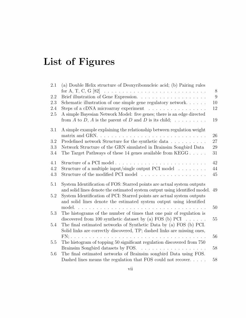
List of Figures
2.1 (a) Double Helix structure of Deoxyribonucleic acid; (b) Pairing rulesfor A, T, C, G [82] . . . . . . . . . . . . . . . . . . . . . . . . . . . . 8
2.2 Brief illustration of Gene Expression. . . . . . . . . . . . . . . . . . . 92.3 Schematic illustration of one simple gene regulatory network. . . . . . 102.4 Steps of a cDNA microarray experiment . . . . . . . . . . . . . . . . 122.5 A simple Bayesian Network Model: five genes; there is an edge directed
from A to D, A is the parent of D and D is its child; . . . . . . . . . 19
3.1 A simple example explaining the relationship between regulation weightmatrix and GRN. . . . . . . . . . . . . . . . . . . . . . . . . . . . . . 26
3.2 Predefined network Structure for the synthetic data . . . . . . . . . . 273.3 Network Structure of the GRN simulated in Brainsim Songbird Data 293.4 The Target Pathways of these 14 genes available from KEGG . . . . . 31
4.1 Structure of a PCI model . . . . . . . . . . . . . . . . . . . . . . . . . 424.2 Structure of a multiple input/single output PCI model . . . . . . . . 444.3 Structure of the modified PCI model . . . . . . . . . . . . . . . . . . 45
5.1 System Identification of FOS: Starred points are actual system outputsand solid lines denote the estimated system output using identified model. 49
5.2 System Identification of PCI: Starred points are actual system outputsand solid lines denote the estimated system output using identifiedmodel. . . . . . . . . . . . . . . . . . . . . . . . . . . . . . . . . . . . 50
5.3 The histograms of the number of times that one pair of regulation isdiscovered from 100 synthetic dataset by (a) FOS (b) PCI . . . . . . 55
5.4 The final estimated networks of Synthetic Data by (a) FOS (b) PCI.Solid links are correctly discovered, TP; dashed links are missing ones,FN; . . . . . . . . . . . . . . . . . . . . . . . . . . . . . . . . . . . . . 56
5.5 The histogram of topping 50 significant regulation discovered from 750Brainsim Songbird datasets by FOS. . . . . . . . . . . . . . . . . . . 58
5.6 The final estimated networks of Brainsim songbird Data using FOS.Dashed lines means the regulation that FOS could not recover. . . . . 58
vii

5.7 The histogram of topping 50 significant regulation discovered from 750Brainsim Songbird datasets by PCI . . . . . . . . . . . . . . . . . . . 59
5.8 The final estimated networks of Brainsim songbird Data using PCI.Dashed lines means the regulation that PCI could not recover. . . . . 59
5.9 The yeast cell cycle pathway inferred from Spellman data using differ-ent methods: (a) FOS (b) PCI (c) Kim [35], and (d) Zhang [85]. . . . 63
viii

Chapter 1
Introduction
1.1 Gene Regulatory Networks
Genes are the basic physical and functional units of heredity. They carry all the
information relevant to what the organism is like, how it survives, and how it behaves
in an environment [67]. Proteins are the building blocks that are essential parts
of living cells. They are the products of genes: a gene will be first transcribed to
an intermediate messenger ribonucleic acid (mRNA), and the mRNA molecule next
translated into a specific protein. Genes in cells do not function individually and
are controlled through intricate interconnections of cellular components, such like
proteins. The gene transcription process is controlled by a collection of proteins
called Transcription Factors (TFs), which can determine when and how much the
specific genes are expressed, and it is also affected by different types of enzymes,
a group of proteins that catalyze reactions [82]. These proteins are production of
corresponding genes, which will then serve as TFs or enzymes that accede to the gene
expression processes of their target genes. The process of genes interacting with each
1

1.2. MOTIVATION 2
other can be described as a Gene Regulatory Network (GRN). Research on GRNs
can provide useful explanations about why the behavior of one gene coincides with
the variations of some other genes.
GRNs are likely the most important organizational level in the cell where inter-
nal signals and the external environment are integrated in terms of corresponding
timed expression levels of genes [10]. They act as biochemical computers in cellular
processes, organizing the level of expression for each gene in the network by control-
ling whether and at what rate that gene will be transcribed. As a result, the type
and amount of proteins are produced differently in different cells in order to make
corresponding cells function properly.
Temporal gene expression data are observations of genetic activity levels over a
number of points of time. The advent of new high throughput technologies, such
as Microarrays, for acquiring gene expression data has made a wealth of molecular
data available. Reverse engineering GRNs, refers to the discovery of the principles
and structures of GRNs using gene expression data; it has received a great deal of
attention in recent years. Computational methods were applied to mine meaningful
interactions between genes.
1.2 Motivation
Reverse Engineering GRNs is an important issue in Bioinformatics, and can yield
remarkable improvements of understanding of biological systems on several fronts:
(i) clarification of and to understand the complex mechanisms of development and
evolution in living organisms [13]; (ii) description of the underlying network structure
of gene regulation pathways [78]; (iii) detection of pathways initiators which are

1.2. MOTIVATION 3
potential reasons of particular genetic disease, and extraction of possible drug targets
[26] and (iv) providing information on possible novel regulations for future research.
Deriving a GRN from gene expression data, however, is often difficult, due to the lack
of complete knowledge of the processes and parameters of the biological system and
its environment.
Numerous computational methods have been developed and investigated to con-
struct GRNs from gene expression data. Popular reverse engineering methods, in-
cludes Association Networks [19, 5], Boolean Networks [31], Bayesian Networks and
Dynamic Bayesian Networks [22, 62]. These methods build upon mathematic or
statistic algorithms to reconstruct networks using correlation, mutual information, or
conditional dependence between genes, respectively. System identification algorithms
are a category of reverse engineering methods that have been applied mainly in en-
gineering domain [57]. GRNs are biological systems that reflect the interconnected
relationships of genes, where temporal measurement of gene expression data can be
obtained as time series signals. Therefore, system identification algorithms have the
ability to build models that reveal the dynamic behaviors of gene regulation. They
fit models of dynamic systems to temporal data, and typically represent quantitative
aspects. These data-driven approaches can construct models from measured input-
output data, giving the best fit to the gene expression data. The inferred models
utilize the target gene in a network as the output and regulating genes as the inputs.
As a result, a structural gene network is obtained. Several system identification ap-
proaches using different models: linear modeling [18, 79], and models consisting of
ordinary differential equations [15, 64], have been discussed recently for inferring gene
regulatory networks.

1.3. OBJECTIVES 4
1.3 Objectives
In this thesis, two system identification algorithms, Fast Orthogonal Search (FOS)
and Parallel Cascade Identification (PCI), are discussed and implemented to build
dynamic models of GRNs. Both FOS and PCI were originally developed for nonlinear
system identification [37, 39], and have been applied in other engineering fields.
Interactive dynamic models of a synthetic dataset, a songbird simulated dataset,
and a real biological dataset, through FOS and PCI are devised. GRNs that capture
the time course variations of genes based on their regulators’ expressions are built for
all the models. The performance of the two approaches is compared with each other,
as well as with other published methods in the literature for verification.
1.4 Contribution
The primary contributions of this work are reported here:
• Two system identification algorithms, FOS and PCI, are presented for building
dynamic models that can capture genetic regulation information. To the best
of the author’s knowledge, neither FOS nor PCI has been used for this purpose
before in the literature.
• A modification on PCI algorithm is proposed. For the case of multiple in-
put/single output system, the original PCI algorithm considers only one input
signal for the dynamic system at a time; multiple input signals are added and
have equal weights. Yet, the modified method is able to treat multiple input
signals simultaneously starting from the dynamic system.

1.5. ORGANIZATION OF THESIS 5
• A method for building a sparse model of gene regulation from PCI is proposed.
As the gene regulatory networks are known to be sparse [48], a fully connected
model does not capture the biological system well.
• Three datasets are used to evaluate and compare the algorithms performances
for capturing GRNs.
– A time-delayed gene regulatory pathway of arbitrary structures was de-
signed. Its corresponding temporal artificial dataset was generated through
a stochastic function.
– A simulated temporal gene expression dataset, was produced using Brain-
sim simulator introduced by [73]. It has 100 genes plus another term
named activity, and represents gene interactions in response to the singing
behavior in a songbird.
– A biological dataset, comprising a subset of yeast Saccharomyces cere-
visiae, which includes the expression levels of 14 cell-cycle regulated genes
over time, were also used.
1.5 Organization of thesis
This thesis is organized as follows. Chapter 2 reviews the fundamental concepts
of molecular biology underlying GRNs. Microarray gene expression measurements
and required preprocessing approaches are discussed. Moreover, a review of related
network inference algorithms is provided. In chapter 3 the datasets that are used for
this study and their required preprocessing steps are introduced. Then in the following
two chapters, a complete description on the theory and implementations of discussed

1.5. ORGANIZATION OF THESIS 6
approaches, Fast Orthogonal Search and Parallel Cascade Identification, are given.
The statistic criteria used for evaluation of each method are also introduced and the
resulting networks are studied to illustrate the performances of discussed algorithms.
Conclusions and future directions of this research are presented in Chapter 6.

Chapter 2
Background
2.1 Basic Concepts in Molecular Biology
A cell is the most basic unit of a organism and also is the smallest unit making up our
bodies. There are tens of thousands of different types of cells, each of which has unique
functions; however, all cells share similarities. The most important shared feature of
cells is that they contain hereditary information in the form of Deoxyribonucleic
acid (DNA) molecular for almost all species1, and have the basic mechanisms for
translating genetic messages into the protein. Proteins are the fundamental structural
and functional units in cells and can act as structural components, enzyme catalysts,
and antibodies [82].
DNA is shaped as a double helix structure shown in Figure 2.1(a), and consists
of two long polymers made from repeating units called nucleotides [82]. These two
polymers are complementary, and the sequence in one strand is completely determined
by the sequence of nucleotides in the other strand. This feature has been recognized
1Some viruses have been discovered that they have RNA genomes.
7

2.1. BASIC CONCEPTS IN MOLECULAR BIOLOGY 8
(a) (b)
Figure 2.1: (a) Double Helix structure of Deoxyribonucleic acid; (b) Pairing rules forA, T, C, G [82]
as one of science’s most famous statements when Watson and Crick first presented
the structure of DNA helix in 1953. The four nucleotides on the DNA, adenine(A),
guanine(G), cytosine(C) and thymine(T), only bond to their complimentary base [82].
Adenine in one strand can only bond with thymine in the other strand, and similarly
guanine has to bond with cytosine, Figure 2.1(b) [82].
A segment of DNA, called a gene, stores genetic codes. A gene consists of a
long combination of four different nucleotide bases. The sequence of nucleotides
in a gene determine the structures of its protein products. According to central
dogma of molecular biology, producing a protein from information in a gene is a two-
step process: transcription and translation. Figure 2.2 summarizes the process of
expressing a protein-encoding gene [82].
The transcription process is to create an equivalent messenger RNA (mRNA) copy
of a portion of DNA. Hence, the information on a gene is transcribed into an mRNA
molecule. An mRNA polymerase enzyme can recognize and bind to a specific site
of DNA molecule, which signals the initiation of transcription. In the translation

2.1. BASIC CONCEPTS IN MOLECULAR BIOLOGY 9
Figure 2.2: Brief illustration of Gene Expression.
step, mRNA produced by transcription is decoded by the ribosome to make a specific
amino acid chain, which later will fold into a protein [82]. This complete process
where a gene gives rise to a protein is called gene expression.
DNA can be compared with a recipe in the gene expression process, due to its
storage of code to instruct other components of cells. Different portions of genes are
active in different cells; as a result their protein products can be drastically different.
The type and amount of proteins produced in each particular cell are extremely
important for the cell to function properly.
The process of gene expression is controlled by a collection of proteins named
transcription factors (TFs). These TFs can decide when, where and at which rate a
particular gene is expressed. Because of the enrollment of different TFs, which them-
selves are protein products of expressed genes, genes are under regulatory control and
comprise complex interactions known as Gene Regulatory Networks (GRNs) [78]. A
brief description is shown in Figure 2.3. Gene1 first is transcribed into mRNA1, and

2.2. MICROARRAYS GENE EXPRESSION MEASUREMENT 10
Figure 2.3: Schematic illustration of one simple gene regulatory network.
then translated to Prontein1 which serves as the TF of Gene2. Therefore, the ex-
pression process of Gene2 is determined by the product of the expression of Gene1,
and Gene1 is defined as its regulator. Furthermore, the expression processes of both
Gene2 and Gene3 are controlled by their common TF, Protein2, which is the expres-
sion product protein of Gene2. Therefore, Gene2 has a self-regulation relationship in
this network, and it also functions as the regulator of Gene3. Once Prontein2 binds
to the specific state of DNA, gene transcription of Gene3 will be activated.
2.2 Microarrays Gene Expression Measurement
Microarrays are a collection of single stranded DNA segments deposited or synthe-
sized on a solid surface. They can monitor the mRNA abundance of genes in a high
throughout fashion [69]. The single stranded DNA segments are called probes and
are complementary to specific RNA species based on the central dogma of molecular
biology [78]. Studies discovered that the amount of mRNA is proportional to the

2.2. MICROARRAYS GENE EXPRESSION MEASUREMENT 11
transcription rate of its corresponding gene [66]. Therefore, the relative transcrip-
tion rate of genes can be calculated through the measurement of their corresponding
mRNA levels. In this section, DNA Microarray experiments are briefly reviewed
because gene expression data has been an important element in advance of reverse
engineering GRNs.
Based on the type of probes used in experiments, Microarrays can be categorized
into two classes, cDNA Microarrays and oligonucleotide Microarrays [70]. cDNA
Microarray is a widely used technology in which two samples are usually analyzed
simultaneously in a comparative fashion. To measure expression levels of genes using
cDNA Microarray, mRNA is extracted from test cell and reference cell, and then
reverse transcribed into cDNA and labeled with fluorescent dyes. The test and ref-
erence cells labeled with dyes that are activated at different frequencies, referred to
as red and green respectively. Two fluorescently labeled samples are then mixed and
the mixture is hybridized on Microarray chips. Finally Microarrays are scanned and
the resulting images are analyzed to calculate gene expression values. The steps of
cDNA microarray is shown in Figure 2.4.
In oligonucleotide Microarray technology, genes on the microarray are represented
by a set of 14 to 20 short sequences of DNA, called oligonucleotide, each of which con-
sists of two probes named perfect match (PM) and miss match (MM). DNA sequences
in every pair of PM and MM are identical, except for one nucleotide in the center of
each sequence. PM is the exact sequence of the selected fragment of the gene. In this
approach, there is no need for using reference samples. First oligonucleotide arrays
are built onto microarray chips. Then mRNA is converted to fluorescently labeled
cDNA followed by hybridization of labeled cDNA samples to Microarray. Finally, the

2.3. PROCESSING MICROARRAY GENE EXPRESSION DATA 12
Figure 2.4: Steps of a cDNA microarray experiment
microarray is scanned and the resulting images are analyzed. Because the correct
gene will only hybridize to the PM, while incorrect hybridization affects both PM
and MM, the expression level of each gene is the average difference between PM and
MM [20]. Affymetrix GeneChip is one of the most widely adopted oligonucleotide
microarray technologies.
2.3 Processing Microarray Gene Expression Data
Due to the effects arising from the variations in the Microarray technologies and ex-
periment setups, preprocessing of gene expression measurements is required for more
reliable data analysis. Accurate preprocessing procedures improve the comparability
of expression data. Microarray data preprocessing usually includes the following steps

2.3. PROCESSING MICROARRAY GENE EXPRESSION DATA 13
[25]:
• Missing Values:
It is estimated that a microarray dataset has more than 5% missing values, af-
fecting more than 60% of the genes [14]. Since many data analysis methods such
as principal component analysis, support vector machines and artificial neural
networks require complete datasets, accurate estimation of missing value is an
important preprocessing step in microarray analysis. Obviously, repetition of
identical experiments can be adopted to solve the missing value issue; however,
this method is costly and time consuming [77]. A series of numerical methods
have been developed to estimate missing values: (1) replacing missing values
with constants; (2) replacing missing values with averages over time [3]; (3) K-
nearest neighbor replacement method [77]; (4) bayesian principal components
analysis replacement method [59]; (5) support vector regression impute method
[80]; (6) least squares formulation based replacement method [34]. Consider-
ing the complexities of different missing values estimation algorithms, simple
averaging is utilized in this thesis.
• Gene Selection:
Gene expression data analysis usually focuses on differentially expressed genes
(DEG). In a microarray experiment, the majority of genes, have constant expres-
sion levels cross time. These genes do not convey any significant information,
on the contrary, they will decrease the efficiency and increase the computational
cost. As such, several methods are developed to select significant genes: the
most simplest way to identify DEGs is by setting a threshold value for detecting
variation of genes; statistic hypothesis tests can also be used for detecting DEGs,

2.4. NETWORK RECONSTRUCTION ALGORITHMS 14
such like t-test [11] and maximal likelihood analysis [27]; fold change analysis,
significant genes can be determined based on relative increase or decrease in
their expression profiles [56].
• Interpolation:
Microarray gene expression dataset usually contains much fewer number of time
points than that of genes. This is partly time consuming nature, and cost of
designing experiment and acquiring data. The accuracies of many temporal
data analysis methods depend on the availability of training samples in time.
Interpolation can increase the number of samples by adding new data points
within the range of original known measurement. Many interpolation methods
are available in numerical analysis [53]: nearest neighbor interpolation, linear
interpolation, spline interpolation, and polynomial interpolation. Appropriate
interpolation can provide more reasonable data samples for analysis.
2.4 Network Reconstruction Algorithms
Given temporal gene expression data acquired under different experimental condi-
tions, a model of the gene interactions can be built through different reverse engi-
neering methods. A gene regulatory network, therefore, is constructed. The GRN is
represented as a graphic model, whose nodes stand for a set of genes and connections
take on different meanings through different models. Providing an accurate reverse
engineering tool that captures a global view of gene regulation is a challenging topic
in Systems Biology.

2.4. NETWORK RECONSTRUCTION ALGORITHMS 15
Many reverse engineering techniques have been proposed for building gene reg-
ulatory networks. Following different criteria, these techniques can be summarized
into several groups. Gardner and Faith [23] used the mathematical graphical models
described them into four categorizations: Association networks, Boolean networks,
Bayesian Networks, and Differential Equations. Karlebach and Shamir [29] roughly
divided various computational models for reverse engineering GRNs into three classes
based on their learning strategies: logical models which allow people to obtain a basic
understanding, continuous models to manipulate behaviors that depending on finer
timing and exact molecular concentrations, and single-molecule level models follow-
ing the observation that the functionality of regulatory networks is often affected
by noise. Another broad classification of deterministic models and stochastic mod-
els, has also been proposed by [68]. Sima [72] reviewed different network inference
methods in two classes based on whether or not they can infer dynamical interaction
between genes. In this section, representative reverse engineering methods, Associa-
tion networks, Boolean networks, and Bayesian Networks, and their advantages and
disadvantages are briefly reviewed. The notation of Genei to describe a gene that is
associated with a random variable Xi, whose gene expression levels are denoted as
Xi(t) at time point t, t = 0, . . . , T .
2.4.1 Association Networks
Association networks are amongst the simplest models for reverse engineering GRNs.
They represent GRNs using an undirected graph with edges weighted by similarities
or relevances. Popular relevance measures are covariance-based measures such as
Pearson correlation, and entropy-based measures such as mutual information.

2.4. NETWORK RECONSTRUCTION ALGORITHMS 16
Pearson correlation, developed by Karl Pearson, is one of the most common and
most useful measures of the linear dependence between two time series variables.
It is a coefficient calculated by dividing the covariance of the two variables by the
product of their standard deviations. The value of the coefficient ranges between −1
and 1. The closer the coefficient is to either −1 or 1, the stronger the correlation
between the variables. If Pearson correlation coefficient is 0, these two variables are
linearly independent. To calculate the Pearson correlation coefficient between two
genes Gene1 and Gene2, the following formula is available
ρ(X1, X2) =
∑Tt=0(X1(t)−X1(t))(X2(t)−X2(t))
T√σX1σX2
, (2.1)
where Xi and σXiare the mean and the standard deviation of random variable Xi,
i = 1, 2.
Pearson correlation only gives a perfect value when two variables are linearly
related. In contrast to this, mutual information, can detect nonlinear correlations. It
is frequently adopted as an index to quantify the mutual dependence of two variables.
The mutual information of two random variables X1 and X2 associate with two genes
is
I(X1;X2) =
T∑t=0
T∑t=0
p(X1(t), X2(t))log
(p(X1(t), X2(t))
p(X1(t))p(X2(t))
), (2.2)
where p(·) is the probability, calculated by the frequencies of corresponding variable.
The greater the mutual information is, the more relevant these two variables are. If
the mutual information is zero, these two variables are irrelevant.
Both Pearson correlation and mutual information have long been used in System
Biology to infer gene regulatory networks. D’haeseleer et al. [19] defined the distance
measure based on residue variance as d(X1, X2) = 1 − ρ(X1, X2)2, where d = 0 if
they are perfectly correlated and d = 1 if they are uncorrelated. Based on mutual

2.4. NETWORK RECONSTRUCTION ALGORITHMS 17
information, a method called ARACNE was proposed by Basso et al. [5], and it has
been used for inferring genetic networks in human B cells. Simplicity and low com-
putational costs are the major advantages of association networks. The limitations
of such models are that they can not reflect causalities and do not take into account
that multiple genes could enroll in the regulation.
2.4.2 Boolean Networks
Boolean Networks were first proposed by Kauffman [31, 30] for the purpose of model-
ing gene regulation, and since then they have been extensively investigated in System
Biology; (1) the mapping to study the qualitative properties of continuous biochemi-
cal control networks using logical structure is further discussed [33, 32]; (2) a model
based on the boolean genetic networks is built as a conceptual framework to identify
new drug targets for cancer treatment [26]; (3) and Liang et al. [50] had described an
algorithm for inferring genetic network from time series of gene expression patterns
using Boolean network model, and Akutsu et al. devises a simpler algorithm for the
same problem [2].
A Boolean network uses binary variables Xi ∈ {0, 1} that denote the tran-
script levels of Genei in the network as ”off” or ”on”, and edges made up of
simple Boolean operations FB, ”AND” ”OR” and ”NOT”. A simple example is
Xi(t + 1) = FBi (X1(t), . . . , XN(t)). The goal of reverse engineering a Boolean net-
work is to find the Boolean function FBi for each gene so that the gene expression
profile can be explained by this model. Two primary strategies were proposed to learn
the connectivity of genes in Boolean Networks. The first one computes the mutual
information between sets of two or more genes and tries to find the smallest set of

2.4. NETWORK RECONSTRUCTION ALGORITHMS 18
input genes that provides complete information on the output gene [50]. The other
one looks for the most parsimonious set of input genes whose expression variations
are coordinated or consistent with the output gene [2].
In contrast to Association Networks, Boolean networks successfully capture the
dynamics of gene regulation. However, Boolean networks are limited because changes
in gene expression levels over time can not be simply represented adequately by two
states and the discritization process from the continuous gene expression levels to
the binary data is not trivial. Furthermore, solving Boolean networks requires large
amount of experimental data because it does not place constraints on the form of the
Boolean interaction functions [23]. To determine a complete set of Boolean functions
from data, all possible combinations of input expression have to be considered. For
a fully connected Boolean network with N genes, it would require approximately 2N
data points to infer all Boolean functions [17] since each gene can be either ”off” or
”on” independently. Both Association networks and Boolean networks are simple ap-
proaches to provide models of gene regulation [6], compared with Bayesian Networks
and System Identification methods that will be discussed.
2.4.3 Bayesian Networks
A Bayesian network(BN) is a probabilistic graphical model that represents a set of
variables and their conditional dependencies via a directed acyclic graph. Such a
model consists of two components, the structure G a directed acyclic graph and the
parameters Θ a set of parameters of conditional distribution of each variable given
the rest of variables. In the graphical structure of the BN given in Figure 2.5, its
nodes stand for genes A,B,C,D,E and edges correspond to conditional dependencies

2.4. NETWORK RECONSTRUCTION ALGORITHMS 19
between genes. The absence of an edge between two genes means that those genes
are conditionally independent given their parent genes, for example, B are D are
conditionally independent given their parent genes A and E. BNs follow the first
order Markov assumption that each variable is conditionally dependent on its parent
only. The joint distribution over the set of genes is also calculated, which can be
rewritten as the product form of probability of each gene given its parents. BNs can
not deal with continuous values. Therefore, the probability of one gene is calculated
by frequencies of discretized expression levels over time.
Figure 2.5: A simple Bayesian Network Model: five genes; there is an edge directedfrom A to D, A is the parent of D and D is its child;
The problem of learning BNs ends up with learning these two components, struc-
ture learning and parameter learning. To construct a BN, using score-based ap-
proaches, is to determine a score function based on posterior probability of BN given
the data, which is then used as the criterion for selecting the optimal set of parents
for each variable. However, this selection procedure is computational costly, because
there are too many possible local structures. Several searching algorithms such like
greedy hill climbing searching [9], simulated annealing searching [49], Markov chain
Monte Carlo [58] and expectation maximization [76], were proposed for learning BNs.

2.4. NETWORK RECONSTRUCTION ALGORITHMS 20
According to the scores of possible structures of proposed BNs by different searching
algorithms, the network G with the greatest conditional probability P (G|D) will be
selected.
Dynamic Bayesian Networks (DBNs), unlike BNs, use temporal gene expression
data for constructing causal relationships among genes. Similar to BNs, the first order
Markov assumption also holds for DBNs. Therefore, the parents of each gene are
selected using information derived from gene expression at the same or the previous
time point, which greatly reduce the complex of DBN learning. As a result, the
structure of DBNs only represents direct associations between genes.
Current methods for DBN learning can be categorized into two major groups,
constraint based methods and score based methods [75]. Constraint based meth-
ods determine conditional independencies and dependencies between genes based on
a statistical tests, which provide satisfactory results with sparse networks [7]. Score
based methods, treat DBN learning as an optimization problem. Such methods devise
a scoring function to evaluate the candidate network structures based on the proba-
bility of the structure given the temporal expression data. They search all possible
network structures and select the optimal one [24].
Both BNs and DBNs have been successfully applied for reverse engineering GRNs
[21, 84, 24, 35, 85]. BNs are not able to reflect the causality or dynamic information
of temporal gene expression data. DBNs can offer a solution, however the complexity
and computational cost is a big bottleneck for analyzing continuous or large datasets
[28].

2.5. SYSTEM IDENTIFICATION METHODS 21
2.5 System Identification Methods
In this thesis, the focus is on a category of reverse engineering gene regulatory net-
works, system identification algorithms. There is no standard definition for the sys-
tem identification methods for reverse engineering gene regulatory networks. System
identification is a term in mathematics and engineering that refers to building dy-
namic models from measured data. Inspired by system engineering and the four
categorizations reviewed in [23], we concluded the definition of system identification
algorithms for reverse engineering GRNs, based on the key different properties of
differential equations compared with the other three categorizations, Association net-
works, Boolean networks, and Bayesian networks. The method that (1) is a dynamic
system capable to deal with continuous temporal expression data, (2) has a deter-
ministic function made up of the expression levels of multiple input genes, (3) is
a quantitative system that can describe the significant affects of regulators accord-
ing to their coefficients of the deterministic function, is called system identification
method. Obviously the differential equation model is an example of system identi-
fication methods. System identification algorithms can be promising tools for the
analysis of genetic systems as they allow for the function description of source genes
with target genes.
Several applications with system identification algorithms on inference of GRNs
have been discussed in the literature that include linear modeling [18, 79], and ordi-
nary differential equations [15, 64].
In a linear model, Genei is modeled as
Xi = β0 +∑j �=i
βjXj , (2.3)

2.5. SYSTEM IDENTIFICATION METHODS 22
where the regression coefficients βj make the model best fit to minimize the least
square error. If Xj is replaced by nonlinear function φ(Xj), where φ is nonlinear
function, the model will be considered a nonlinear one. To model the dynamics from
gene expression data, the above equation eq(2.3) can be written as
Xi(t) = β0 +∑j �=i
βjXj(t− 1). (2.4)
Such models represents that the change in the expression level of one gene at time
point t depends on a weighted linear sum of the expression levels of its regulator
genes at previous time point t − 1. One of the properties of linear models is that
each regulator contributes to the output independently of the rest of the regulators,
in the mathematical summation manner [29]. Linear models do not require a prior
knowledge about regulatory mechanisms. There are a series articles using linear
modeling to construct GRNs in the literature [4, 12, 18, 81, 83].
Ordinary differential equations (ODEs), are amongst the most popular formalisms
to model dynamic systems in science and engineering, and have also been used for
reverse engineering GRNs [15, 64]. ODEs model the gene expression profiles, where
the regulatory interaction takes the form of functional and differential relations be-
tween the gene expression profiles. More specifically, the ODE has the mathematical
form,
dXi
dt= αi + fi(X), i = 1, . . . , N, (2.5)
where fi is the corresponding function of Genei, and X is the matrix indicating all
the gene expression profiles, Gene1, · · · , GeneN . Obviously, ODEs can also take into
account time lag arising from the time required, Xi on the LHS of eq(2.5) is replaced
with Xi(t) and X on the RHS is replaced with X(t − 1). Since functions fi are not

2.5. SYSTEM IDENTIFICATION METHODS 23
fixed, many studies have used different functions such as sigmoidal functions were
used in [81] and linear functions in [8]. ODEs provide detailed information about the
dynamic of gene expression data.
Fast Orthogonal Search (FOS) uses orthogonal searching to identify the significant
regulators in describing the output. It iteratively searches a given candidate function
set, selects and adds the most significant function term to build up the model. Parallel
Cascade Identification (PCI) utilizes a number of cascades, each of which is a smaller
system, to solve system identification problem. The difference between system output
and the first cascade output is treated as the output of the new system for adding a
second cascade. The difference is again computed and another cascade is added. this
process continues until it reaches a desired approximation error. These two system
identification algorithms, have been extensively implemented in many different fields,
but not in reverse engineering gene regulatory networks. FOS has been applied to
estimate raman spectral [42], to detect broken rotor bar in motor [63] or estimate AC
induction motors [52], to select features for computer-aided diagnosis of breast cancer
[65], and to estimate optimal joint angle for upper limb hill muscle models [55]. PCI
is also a popular method that has been studied in signal classification [44], and to
predict clinical outcome or metastatic status [40, 41]. Especially they were used to
analyze genetic data, to predict the response of multiple sclerosis patients to therapy
using FOS [54] and to classify and predict protein family using PCI [43, 46]. The
two algorithms discussed in this thesis, FOS and PCI, could be considered as two
particular linear models, and if self-regulation is permitted, could also be considered
as two particular ordinary differential equation models.

Chapter 3
Data and Preprocessing
To evaluate the proposed approaches for reverse engineering gene regulatory net-
works, three different datasets are employed. First, a temporal synthetic dataset is
developed and used for evaluating the performance of FOS and PCI. Second, these
two methods are applied to songbird data which is a known simulated temporal gene
expression dataset developed by Smith et al.[73]. This dataset includes gene reg-
ulatory information with response to the singing behavior of a songbird. Since its
gene regulatory network is known, it is a good benchmark for evaluating the reverse
engineering methods. Finally, a real biological dataset from yeast Saccharomyces
Cerevisiae cell cycle is used. This dataset is a subset from a study by Spellman et
al.[74], including 14 genes. The cell-cycle pathway of these 14 genes is available in
KEGG1. Saccharomyces Cerevisiae yeast data has been studied both biologically and
using computational methods in the literature, which provides us with a great deal
of information for evaluating the performances of proposed methods. These three
1KEGG: Kyoto Encyclopedia of Genes and Genomes is a bioinformatics resource that storesgenomic and molecular knowledge.
24
3.1. DATA 25
datasets are referred to as the synthetic data, the songbird data, and the yeast data
in the remain of this thesis.
In this chapter, these datasets will be introduced and the necessary preprocessing
steps are explained prior to further analysis of the data.
3.1 Data
3.1.1 Temporal Synthetic Data
One time-delayed gene regulatory network of an arbitrary structure is modeled to
assess how well FOS and PCI can be used for learning the genetic connections. Based
on the network, a regulation weight matrix is generated and used to simulate tem-
poral expression data. All simulations are done using MATLAB. After the temporal
expression dataset is obtained, both FOS and PCI are used to learn it and construct
two estimated networks, respectively. The calculated networks are then compared
with the actual network to evaluate their performances.
An important assumption made in generation of this dataset is that the expression
level of a regulator gene at time point t only determines the expression value at next
time point t+ 1 of its target gene. The following stochastic formula holds:
Xt+1 = R ∗Xt + E, t = 0, . . . , T. (3.1)
where Xt+1 and Xt are column vectors which denote the expression levels of all genes
at corresponding time points t + 1 and t; E is a vector of system noise; R is the
regulation weight matrix representing gene regulations.
If there is a regulatory relationship directed from source gene i and target gene j,
the entry Rij of R is a nonzero number; otherwise it is zero. It is not difficult to notice
3.1. DATA 26
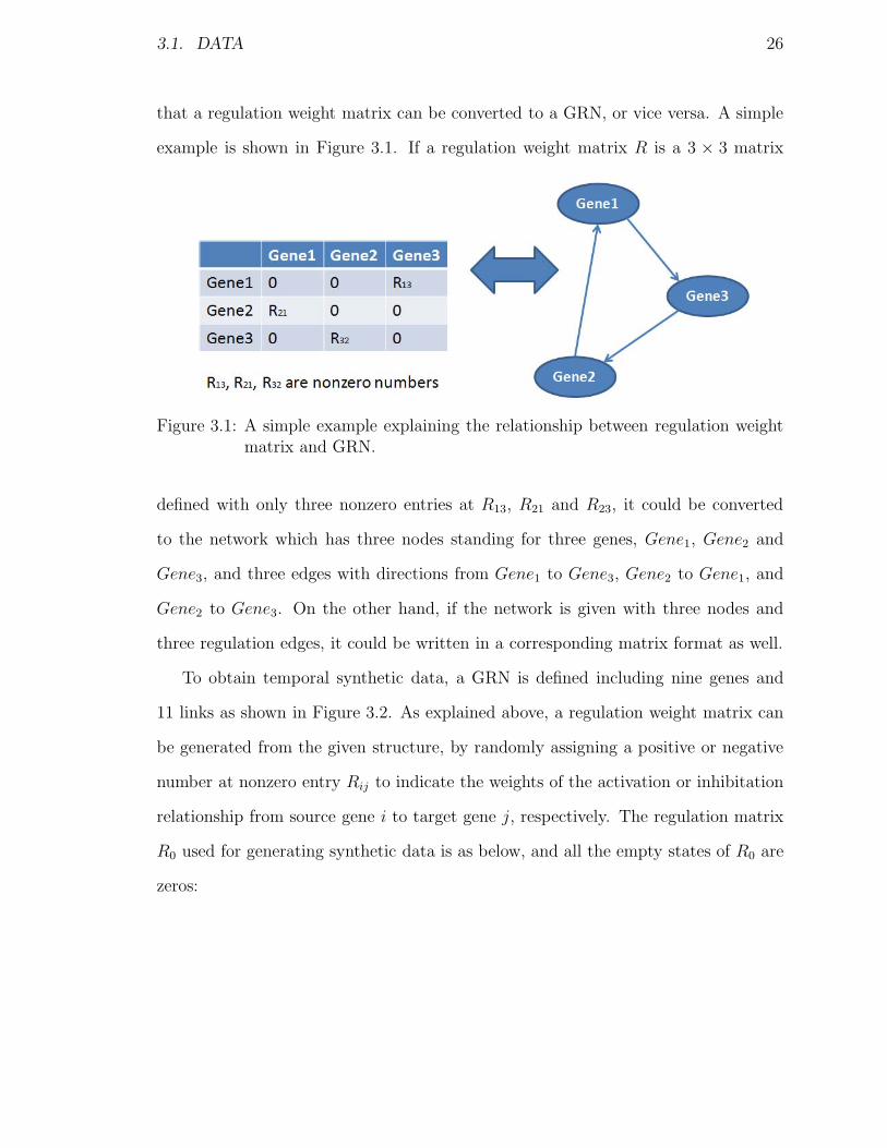
that a regulation weight matrix can be converted to a GRN, or vice versa. A simple
example is shown in Figure 3.1. If a regulation weight matrix R is a 3 × 3 matrix
Figure 3.1: A simple example explaining the relationship between regulation weightmatrix and GRN.
defined with only three nonzero entries at R13, R21 and R23, it could be converted
to the network which has three nodes standing for three genes, Gene1, Gene2 and
Gene3, and three edges with directions from Gene1 to Gene3, Gene2 to Gene1, and
Gene2 to Gene3. On the other hand, if the network is given with three nodes and
three regulation edges, it could be written in a corresponding matrix format as well.
To obtain temporal synthetic data, a GRN is defined including nine genes and
11 links as shown in Figure 3.2. As explained above, a regulation weight matrix can
be generated from the given structure, by randomly assigning a positive or negative
number at nonzero entry Rij to indicate the weights of the activation or inhibitation
relationship from source gene i to target gene j, respectively. The regulation matrix
R0 used for generating synthetic data is as below, and all the empty states of R0 are
zeros:

3.1. DATA 27
Figure 3.2: Predefined network Structure for the synthetic data
R0 =
⎛⎜⎜⎜⎜⎜⎜⎜⎜⎜⎝
1 1-0.6
-1 -11 -4
11
-21
⎞⎟⎟⎟⎟⎟⎟⎟⎟⎟⎠
To simulate the synthetic dataset, first all gene expression levels are initialized
as zeros. Because Gene4 has no regulators, its expression levels are assigned with a
series of random real numbers. The expression levels of all genes are generated using
their regulators, and corresponding weight in R0 using eq(3.1), where the values of
noise E are assigned by MATLAB command randn which generates samples of a
standard normal distributed random variable. The expression values of all genes
are generated recursively over 150 time points. To study the transient response of
regulation, the data starting from the 50th time point is kept to further studies.
One hundred synthetic datasets are simulated by repeating this procedure. The only
differences among all synthetic datasets are the influences of noise value E in eq(3.1).

3.1. DATA 28
3.1.2 Brainsim Songbird Dataset
To provide a suitable way for evaluating network inference algorithms, Smith et al [73]
designed the Brainsim simulator2 to generate data representing a complex biological
system. Brainsim models the vocal communication system of the songbird brain.
The brain of a songbird is modeled as five regions, where the expression levels of
one hundred genes and the activity level in each of these regions of the brain are
simulated. A bird exhibits a behavior, in two possible states, 0 or 1 representing
”Silence” or ”Singing”.
The singing behavior of a songbird will cause a variation in the activity level,
which will directly affect the expression levels of involved genes in the network. This
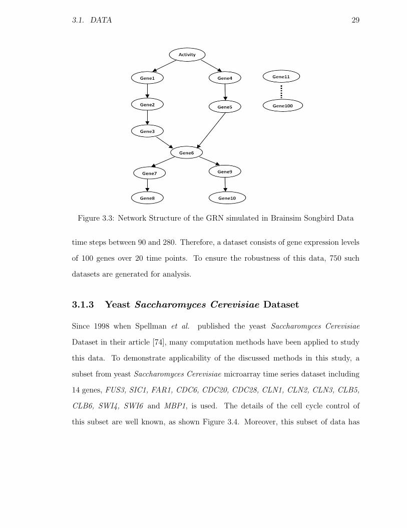
gene regulatory network in every region contains 100 genes; however, only 10 of these
genes are connected with each other and correspond to the singing behavior. Two
of these ten genes, named as Gene1 and Gene4 are directly affected by the activity
level, and they affect the expression levels of the remaining eight genes as shown in
Figure 3.3. However, the remaining 90 genes are irrelevant, and can be considered as
noise.
The expression levels of the ten relevant genes at each time point are determined
by the expression levels of their regulators, noise, and a degradation factor. The 90
irrelevant genes expression levels randomly fluctuate or attenuate within the upper
and lower expression level bounds, from 0 to 50. Since noise is modeled in the
simulator, every time a gene expression dataset is generated, it will differ slightly
from the previous data but reflect the same gene regulatory network. The sampled
activity and gene expression data points are taken at the sampling interval of ten
2The Brainsim simulator and the songbird data are available online http://biology.st-andrews.ac.uk/vannesmithlab/downloads.html.
3.1. DATA 29
Figure 3.3: Network Structure of the GRN simulated in Brainsim Songbird Data
time steps between 90 and 280. Therefore, a dataset consists of gene expression levels
of 100 genes over 20 time points. To ensure the robustness of this data, 750 such
datasets are generated for analysis.
3.1.3 Yeast Saccharomyces Cerevisiae Dataset
Since 1998 when Spellman et al. published the yeast Saccharomyces Cerevisiae
Dataset in their article [74], many computation methods have been applied to study
this data. To demonstrate applicability of the discussed methods in this study, a
subset from yeast Saccharomyces Cerevisiae microarray time series dataset including
14 genes, FUS3, SIC1, FAR1, CDC6, CDC20, CDC28, CLN1, CLN2, CLN3, CLB5,
CLB6, SWI4, SWI6 and MBP1, is used. The details of the cell cycle control of
this subset are well known, as shown Figure 3.4. Moreover, this subset of data has

3.1. DATA 30
been extensively explored before, allowing for a comparison with those results in the
literature [35] and [85].
These 14 genes are involved in the early cell cycle of the yeast Saccharomyces
cerevisiae (budding yeast). Cell cycle is the series of events that takes place in a cell
leading to its division and duplication [82]. In yeast, it is accomplished through a
reproducible sequence of events, DNA replication (S phase) and mitosis (M phase)
separated temporally by gaps, G1 and G2 phases. At G1 phase, CDC28 associates
with CLN1, CLN2 and CLN3, while CLB5 and CLB6 regulates CDC during S, G2,
and M phases [1]. The activity of CLN3/CDC28 is required for cell cycle progression
to start. When the levels of CLN3/CDC28 accumulate more than a certain threshold,
SWI4/SWI6 and MBF1/SWI6 are activated, promoting transcription of CLN1 and
CLN2 [1]. CLN1/CDC28 and CLN2/CDC28 promote activation of other associated
kinase, which drives DNA replication SIC1 and FAR1 are the substrates and inhibitors
of CDC28. CDC6 and CDC20 affect the cell division control proteins. Mitogen-
activated protein kinase affect this progression through FUS3.
Kyoto Encyclopedia of Genes and Genomes (KEGG) contains all the current
knowledge of molecular and genetic pathways based on experimental observations
in organisms. KEGG regulatory pathway represents the current knowledge on the
protein and gene interaction networks [60]. The structure of the KEGG pathway of
the above-mentioned 14 genes is already given (Figure 3.4), and also it is considered
as the target network in this thesis.
The available dataset online3 generated by Spellman et al. [74] contains three time
series which were measured using different cells synchronization methods: α factor-
based arrest (referred to as alpha, includes 18 time points at 7 minutes interval over
3Data is available online http://genome-www.stanford.edu/cellcycle/

3.2. PREPROCESSING 31
Figure 3.4: The Target Pathways of these 14 genes available from KEGG
119 minutes), size-based (elu, 14 time points at 30 minutes interval over 390 minutes),
and arrest of a cdc15 temperature-sensitive mutant (cdc15, 24 time points, first 4 and
last 3 of which are at 20 minutes interval and the rest are at 10 minutes interval over
290 minutes). The alpha dataset is used and then studied in more detail as it was
also used in two previous studies [35, 85].
3.2 Preprocessing
In order to remove systematic bias in datasets, the preprocessing methods are neces-
sary to prepare the data for later analysis [51]:
• Removing outliers
• Replacing missing values

3.2. PREPROCESSING 32
3.2.1 Outlier Correction
Outliers in the gene expression data are the values that are far away from most of the
other values, which means such entries have a high probability of being incorrectly
obtained. To discover the outliers, statistic hypothesis that the expression levels of
a gene in different experiments are supposed to distribute in the range of twice its
standard deviation, σ, distance from its mean, μ is employed. All expression values
therefore greater than μ+2σ or less than μ− 2σ are considered as outliers. Detected
outliers of gene i will be removed and replaced by the mean μi of its expression
values over experiments. There are 100 replicates for the synthetic data (750 for the
songbird data), and less than 2% (1.8%) outliers were detected over all experiments.
Therefore, the effects of outliers can be ignored.
3.2.2 Missing Values
The yeast Saccharomyces Cerevisiae data in our studies have several missing values.
These missing values could be due to unreliable measurements at certain time points.
The other two datasets, synthetic data and songbird data, devised from computational
simulation, can avoid missing values by setting appropriate parameters. In this work,
the mean of each gene expression value over time is used to fill in the positions of
missing entries in the expression data of the yeast dataset, as mean is a statistically
sound measure and easy to implement.

Chapter 4
Methods
In this chapter, Fast Orthogonal Search (FOS) and Parallel Cascade Identification
(PCI) are introduced for reverse engineering of gene regulatory networks, and their
implementation is discussed.
To reverse engineer a network, one gene is studied at one time, and treated as the
system output, and the remaining genes are considered as system inputs. Through
the proposed algorithms, significant input genes can be selected from the pool of
all possible ones and used as the regulators of the corresponding output to build a
network. Both FOS and PCI were developed for system identification [37, 39]. They
have been applied to predict the response of multiple sclerosis patients to therapy
using FOS [54] and to classify and predict protein family using PCI [43, 46].
4.1 Fast Orthogonal Search
Fast Orthogonal Search was developed for identifying a model by searching through
a set of pre-designated candidate functions and iteratively selecting the optimal term
33

4.1. FAST ORTHOGONAL SEARCH 34
that produces the maximum reduction of mean square error (MSE) of the model
[37, 38]. Different from traditional orthogonal search algorithms eg. [36], the search-
ing procedure in FOS could avoid calculating the actual values of orthogonal terms,
which greatly speeds up the approximation procedure. It was shown that, compared
with an orthogonal search algorithm by Desrochers [16], whose computational cost
is proportional to the square of the number of candidate functions, FOS depends
linearly on the number of candidate functions [37].
4.1.1 Orthogonal Search
An approximation of a dynamic system over t = 0, · · · , T can be shown using the
following equation as:
y(t) = F [y(t− 1), . . . , y(t−K), x(t), . . . , x(t− L)] + e(t), t = 0, · · · , T, (4.1)
where y(t) is the system output; F is a polynomial function; x(t) is the input and e(t)
is error; K and L are the time delay of input and output, respectively. This equation
can be rewritten in a concise format:
y(t) = c+
M∑m=1
ampm(t) + e(t), t = 0, . . . , T, (4.2)
where c is a constant, pm(t) form = 1, 2, . . . ,M are the non-orthogonal basis functions
selected to be added to the model, and am are the associated coefficients which best
fit the output. The basis functions pm(t) have the following form
pm(t) = y(t− k1) · · · y(t− ki)x(t− l1) · · ·x(t− lj), m ≥ 1, (4.3)
where 1 ≤ k1, · · · , ki ≤ K, i ≥ 0 and 0 ≤ l1, · · · , lj ≤ L, j ≥ 0.

4.1. FAST ORTHOGONAL SEARCH 35
Through Gram-Schmidt orthogonalization [61], eq(4.2) can be rewritten as:
y(t) = c+
M∑m=1
gmwm(t) + e(t), t = 0, . . . , T, (4.4)
where wm(t) for m = 1, . . . ,M are orthogonal functions over the data and gm are the
orthogonal expansion coefficients, achieving a least-square fit. The constant c can be
considered as a zero-order function that equals 1, with a coefficient g0 = c. Therefore,
c = g0w0(t) where w0(t) = 1, t = 1, . . . , T . Since wm(t) are mutually orthogonal over
the data record and derived from pm(t), the orthogonal search algorithm iteratively
constructs a function which is orthogonal to all previously selected terms,
wm(t) = pm(t)−m−1∑r=0
αmrwr(t), m = 1, . . . ,M
where αmr =pm(t)wr(t)
w2r(t)
.1 Orthogonal search is efficiently used to select model terms
to develop models of the above form.
On the other hand, looking for optimal am in eq(4.2) minimizing the mean square
error (MSE) of the system:
error =
(y(t)− c−
M∑m=1
ampm(t)
)2
(4.5)
is equivalent to looking for optimal gm in eq(4.4) to minimize its MSE
error =
(y(t)−
M∑m=0
gmwm(t)
)2
= y2(t)−M∑
m=0
g2mw2m(t) (4.6)
due to the mutual orthogonal property of wm. To find the optimal gi that best fits
1The over-bar in section 4.1 always denotes the time average over the data from time R =max(K,L) to t = T , where T is the length of the time series.

4.1. FAST ORTHOGONAL SEARCH 36
the data, we take the first derivative of eq(4.4) [71],
error′ =
⎧⎨⎩(y(t)−
M∑m=0
gmwm(t)
)2⎫⎬⎭
′
= 2
⎧⎨⎩(y(t)−
M∑m=0
gmwm(t)
)× (−wi(t))
⎫⎬⎭
= 2
⎧⎨⎩y(t) (−wi(t)) +
(M∑
m=0
gmwm(t)
)wi(t)
⎫⎬⎭
= 2{−y(t)wi(t) + giwi(t)wi(t)
}. (4.7)
By assigning eq(4.7) with 0, the value of gm is given by:
gm =y(t)wm(t)
w2m(t)
, m = 0, . . . ,M. (4.8)
Now the coefficients am in eq(4.2) can be calculated by
am =M∑i=m
giυi, (4.9)
where
υm = 1, υi = −i−1∑r=m
αirυr, i = m+ 1, . . . ,M.
It is shown that the reduction in MSE by adding any given candidate func-
tion is readily obtained from the norm of the corresponding orthogonal function
and the orthogonal expansion coefficient. Assume that M candidate function terms
p1(t), · · · , pM(t) have already been selected to estimate the output, a further one
aM+1pM+1(t) is to be added to the right side of eq(4.2), i.e., a corresponding orthog-
onal function term gM+1wM+1 is to be added on the right side of eq(4.4), the MSE of
the model will be reduced by:
Q(M + 1) = g2M+1w2M+1(t). (4.10)

4.1. FAST ORTHOGONAL SEARCH 37
Therefore the candidate function term that is associated with the greatest Q is
the function term causing the maximum reduction of MSE. This function term will
be selected and added this to eq(4.2). This process is repeated iteratively until no
further terms could reduce the MSE by more than a given threshold, or if a maximum
number of accepted terms is reached. This process will result in an accurate model
that can describe the data. However the creation of calculating orthogonal functions
wm(t) is costly as mentioned in the beginning. Therefore, Fast Orthogonal Search
(FOS) is introduced to solve this problem.
4.1.2 Fast Orthogonal Search
Recall the introduced formulas above, to build the model of eq(4.2),
1. am is calculated using eq(4.9), where gm is given byy(t)wm(t)
w2m(t)
,
2. wm is calculated using pm(t)−m−1∑r=0
αmrwr(t),
3. αmr =pm(t)wr(t)
w2r(t)
,
4. Q(M) = g2Mw2M(t).
after comparison of the three equations, it is not difficult to see that all of the numer-
ators and the denominators are cross productions of corresponding terms, and the
denominator of αmr is similar to that of gm. FOS uses a vector C(m) and a matrix
D(m,m) to calculate the numerator and denominator of gm, respectively. Moreover,
the second part of Q(M) has a similar property, and can be substituted by D(r, r).

4.1. FAST ORTHOGONAL SEARCH 38
Therefore, the significant function terms can be selected using Q(M) and their corre-
sponding function coefficients am can be calculated without calculating the orthogonal
function terms wm(t).
Given a candidate function set with M terms, he pseudocode to calculate the vec-
tor C and the matrixD through FOS as presented in [38] is given below:
START
D(0, 0) = 1
C(0) = y(t)
for m = 1 to M do
Calculate D(m, 0) = pm(t)
end for
for m = 1 to M do
for r = 0 to m− 1 do
Calculate α using αmr = D(m, r)/D(r, r)
CalculateD(m, r+1) usingD(m, r+1) = pm(n)pr+1(n)−∑r
i=0 αr+1iD(m, i)
end for
Calculate C(m) = y(n)pm(n)−∑m−1
r=0 αmrC(r)
end for
After C and D are available, gm could be calculated by using eq(4.11).
gm =C(m)
D(m,m), for m = 0, . . . ,M. (4.11)
It has been proved in [37] by Korenberg that the MSE of the model defined by
eq(4.5) can be expressed as follows:
error = y2(t)−M∑
m=0
g2mD(m,m). (4.12)

4.1. FAST ORTHOGONAL SEARCH 39
Comparing eq(4.7) and eq(4.12), Q(M + 1) in eq(4.10), the amount of reduction of
MSE by adding a new term aM+1pM+1(t), is of this form
Q(M + 1) = g2M+1D(M + 1,M + 1). (4.13)
To select the (M+2)th term pM+2(t) we only need to carry out the above procedure
for m = M + 2. We do not need to repeat previous calculations for m ≤ M + 1. As
mentioned above, FOS will continue to select and add the optimal candidate term
to reduce the MSE of the model until it reaches some stopping criteria. In [37, 38],
two stopping criteria have been mentioned to terminate FOS. One is that once all
candidate function terms have been selected from the candidate functional set, FOS
will stop searching. The other one is based on a statistic significance test: FOS will be
terminated if adding a further term can not reduce MSE more than white gaussian
noise. Suppose we already selected M terms, for a given candidate function term
pM+1(t), its corresponding value of Q(M+1) can be calculated by eq(4.13). It can be
shown that if e(t) is a zero-mean, independent Gaussian noise, then the correlation
coefficient r is given by
r =
(Q(M + 1)
y2(t)−∑Mm=0 Q(m)
) 12
<2√
T − R + 1, (4.14)
with probability of around 0.95 confidence interval (C.I.) for sufficiently long record
length T − R + 1 [71]. Note that the denominator of R.H.S. of eq(4.14) is the stan-
dard deviation of r. Moreover, here 2 is an approximated value of 1.96, based on
− 1.96√T − R + 1
< r <1.96√
T − R + 1. Therefore, eq(4.14) can be rewritten in a more
general way:
Q(M + 1) >K
T − R + 1
(y2(t)−
M∑m=0
Q(m)
). (4.15)
4.1. FAST ORTHOGONAL SEARCH 40
For example, if we set K = 4, FOS will end up with a 95% C.I. [45] and if K is
chosen as 10.9, the C.I. will be 99.9% [42].
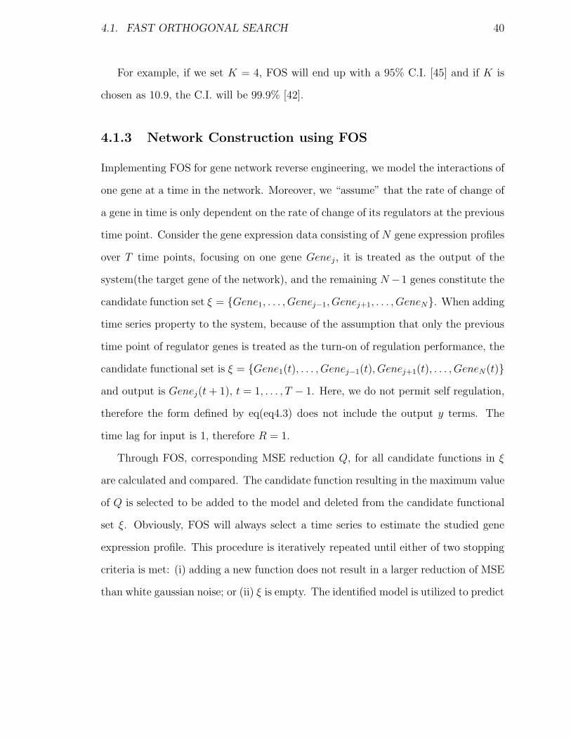
4.1.3 Network Construction using FOS
Implementing FOS for gene network reverse engineering, we model the interactions of
one gene at a time in the network. Moreover, we “assume” that the rate of change of
a gene in time is only dependent on the rate of change of its regulators at the previous
time point. Consider the gene expression data consisting of N gene expression profiles
over T time points, focusing on one gene Genej , it is treated as the output of the
system(the target gene of the network), and the remaining N−1 genes constitute the
candidate function set ξ = {Gene1, . . . , Genej−1, Genej+1, . . . , GeneN}. When adding
time series property to the system, because of the assumption that only the previous
time point of regulator genes is treated as the turn-on of regulation performance, the
candidate functional set is ξ = {Gene1(t), . . . , Genej−1(t), Genej+1(t), . . . , GeneN(t)}and output is Genej(t+ 1), t = 1, . . . , T − 1. Here, we do not permit self regulation,
therefore the form defined by eq(eq4.3) does not include the output y terms. The
time lag for input is 1, therefore R = 1.
Through FOS, corresponding MSE reduction Q, for all candidate functions in ξ
are calculated and compared. The candidate function resulting in the maximum value
of Q is selected to be added to the model and deleted from the candidate functional
set ξ. Obviously, FOS will always select a time series to estimate the studied gene
expression profile. This procedure is iteratively repeated until either of two stopping
criteria is met: (i) adding a new function does not result in a larger reduction of MSE
than white gaussian noise; or (ii) ξ is empty. The identified model is utilized to predict

4.2. PARALLEL CASCADE IDENTIFICATION 41
Genej using the selected genes, which are defined as regulators of Genej . Once all
the genes Genej , j = 1, . . . , N have been studied as the target, a network consisting
of all genes is constructed, whose nodes stand for genes, edges denote the regulations
between genes and arrows of the edges describe the direction of the regulation. Note
that the model built through FOS is highly dependent on the predefined candidate
basis function set. One could define complex basis functions like cross-products to
construct a more complicated network.
4.2 Parallel Cascade Identification
Parallel Cascade Identification (PCI) builds a model of input/output relationship of a
system using a number of cascades, each of which has a dynamic component, capable
to capture the memory of a system, followed by a static polynomial component, which
enables an accurate estimation of the system output, as shown in Figure 4.1 [39].
PCI starts by approximating the system utilizing the first cascade. The difference
of the actual system output, y(t), with the first cascade output, z1(t), is called the
residue, y1(t). The residue is then treated as the output of a new system that will
be approximated by the second cascade. The residue is again computed, and another
cascade is added. The process continues until it reaches a desired threshold for the
approximation error.
For a system represented as eq(4.1), following the Stone-Weierstrass theorem [47],
it can be approximated with a finite order Volterra series2, that is
ys(n) = k0 +M∑
m=1
Vm, n = 0, 1, . . . (4.16)
2The Volterra series were developed in 1887 by Vito Volterra. It is a model for non-linear behavior,similar to the Taylor series. But it has the ability to capture ‘memory’ effects.

4.2. PARALLEL CASCADE IDENTIFICATION 42
Figure 4.1: Structure of a PCI model
where M is the order of the Volterra series and for m ≥ 1, the mth order Volterra
functional is of this form
Vm =
R∑i1=0
· · ·R∑
im=0
km(i1, . . . , im)x(n− i1) · · ·x(n− im), (4.17)
where km is the mth order symmetric Volterra kernel which can be seen as a higher
order impulse response of the system and R + 1 is the memory length, which means
that the series output ys(n) only depends on input delays from 0 to R lags.
Consider a time series y(t) as the system output and x(t) as the input, t = 0, . . . , T ,
and assume that y(t) depends on input delays from 0 to R, PCI starts with the first
cascade to approximate the system. Let yi(t) be the residue after the ith cascade has
been added to the parallel cascade model. Thus, y0(t) = y(t). Obviously, following
its definition, the following equation holds:
yi(t) = yi−1(t)− zi(t), i = 1, 2, . . . . (4.18)
Consider fitting the ith cascade to the residue yi−1(t), i = 1, 2, · · · , the procedure

4.2. PARALLEL CASCADE IDENTIFICATION 43
of PCI is shown in Figure 4.1 and could be briefly described as follows:
1. Define a candidate function pool hi for a possible impulse response of the
dynamic system in the ith cascade and is of length R. hi consists of cross-
correlation functions of different orders between the input, x(t), and the residue,
yi−1(t). The cross-correlation functions are computed over a segment of the in-
put and output signals extending from t = R to t = T . For example, the
first-order cross correlation function is
φxyi−1(j) � 1
T − R + 1
T∑t=R
yi−1(t)x(t− j), and (4.19)
2. Randomly select the impulse response hi(j) from the pre-defined candidate
function pool, and the output of the dynamic component, ui(t), is calculated
by the following equation:
ui(t) =R∑
j=0
hi(j)x(n− j). (4.20)
3. ui(t) is then treated as the input of the static system. By fitting a static P(·)from the input ui(t) to the residue yi−1(t), a cascade is completely constructed.
The cascade output zi(t) = P[ui(t)].
4. Calculate the MSE of the estimated model, i.e. the mean square value of the
new residue over t = R, . . . , T , y2i (t) = (yi−1(t)− zi(t))2 = y2i−1(t)− z2i (t).
5. Repeat this procedure until MSE reduction caused by adding new cascade is
less than a threshold. Similar to the stopping criteria of FOS, when trying to
add a further cascade, the correlation coefficient r =
√z2i+1(t)/y
2i (t) is required
to follow |r| < 2/√T −R + 1 with probability of around 95%.

4.2. PARALLEL CASCADE IDENTIFICATION 44
Prior to reverse engineering GRNs using PCI, the multiple-input case is necessary
to be discussed. The multiple inputs case introduced in [39] is briefly reviewed here,
and shown in Figure 4.2. For example, consider two input signals, x1(t) and x2(t),
Figure 4.2: Structure of a multiple input/single output PCI model
the differences of PCI procedure from the single input case are:
• In Step 1, the candidate set for impulse response will also include a further
term, the cross-correlation of residue yi−1 with both x1(t) and x2(t).
• In Step 2, to include both inputs in the system, the output of linear system is
calculated by
wi(t) = ui(t)± Cx2(t− A), (4.21)
where the sign is chosen randomly, C is a convergent constant defined as
y(i−1)2(t)
y2(t), and the integer A is selected randomly from 0, · · · , R.
To include three or more inputs in the system, the output of linear system is calculated

4.2. PARALLEL CASCADE IDENTIFICATION 45
by
wi(t) = ui(t)±∑i
≥ 2Cxi(t− Ai), (4.22)
where Ai is randomly selected from {0, . . . , R} and C follows the previous definition.
4.2.1 Network Construction using PCI
For reverse engineering of gene networks, the time lag is set as R = 1. To approximate
the system, for the multiple-input case, if all input genes are assigned the same
coefficients C, even though an acceptable mathematical model can be generated to
predict the time series of the output, this model is not a good representation of genetic
regulation. Since PCI randomly selects the impulse response, here a modification is
made to PCI in this work as shown in Figure 4.3. First the system output y(t)
Figure 4.3: Structure of the modified PCI model
is the gene expression levels of Genej over time, and the input of the system is
X(t) = {Gene1(t), . . . , Genej−1(t), Genej+1(t), . . . , GeneN (t)}. Constructing the ith

4.3. ASSESSMENT OF NETWORK INFERENCES 46
cascade, every time we generate a vector Hi of impulse responses corresponding to
the input vector instead of only one impulse response in the original PCI. Assuming
R = 1, the output of the dynamic system is ui(t) = HiX(t− 1), and is directly used
as the input of static polynomial system.
Empirical data indicate that gene regulatory networks should be sparse, and the
average number of upstream regulators of per gene is less than two [48]. Unlike FOS
in which a criteria can be set to terminate the procedure once the maximum number
of accepted regulators is met, PCI will generate a relatively full matrix, except for its
diagonal (which are zeros as self-regulation is not allowed in the models). A method
is developed to reduce the number of estimated links by PCI. The regulation from
Genei to Genej is defined significant if the entry Rij of the regulation weight matrix
R has a greater absolute value compared with all the rest of the entries in the same
column. For example, if Rij is outside of the range of k standard deviation from the
mean of the corresponding column, it will be kept for further studies.
4.3 Assessment of Network Inferences
In order to evaluate the performances of the proposed methods, FOS and PCI, for
identifying gene regulatory networks from the datasets, statistical measures are em-
ployed for this purpose. For predictive analysis, confusion matrix (Table 4.1), is a
table with two rows and two columns that reports the number of True Positives, False
Positives, True Negatives and False Negatives.
• True Positive (TP): the interaction that exists in both the actual network and
inferred network by the reverse engineering methods;

4.3. ASSESSMENT OF NETWORK INFERENCES 47
Table 4.1: Confusion Matrix
actual links total
predicted linksTrue Positives False Positives P’
False Negatives True Negatives N’
total P N
• False Positive (FP): the interaction that does not exist in the actual network
but was falsely inferred by reverse engineering methods;
• True Negative (TN): the interaction that does not exist in either the actual
network or the inferred network;
• False Negative (FN): the interaction that does exist in the actual network but
is not inferred by the reverse engineering methods.
Moreover, three other criteria Precision (pre), Sensitivity (sen) and Specificity (spc)
are also employed as the evaluation methods, and defined as
precision =TP
TP + FP=
# of correctly estimated interactions
# of all estimated interactions,
sensitivity =TP
TP + FN=
# of correctly estimated interactions
# of all actual interactions,
specificity =TN
TN + FP
=# of possible interactions do not exsit in actual or estimated networks
# of possible interactions do not exsit in the actual network.

Chapter 5
Implementation and Results
Both FOS and PCI are implemented using MATLAB. In this chapter, details of their
implementations and the results of reverse engineered networks using each dataset,
described in Chapter 3, are provided. First, the temporal synthetic dataset is used
to evaluate the performances of FOS and PCI. Then, Brainsim songbird data will be
analyzed and its resulting networks will be compared with the actual network. In the
end, FOS and PCI will be applied on the yeast datasets and the inferred networks
will be compared with the target network from KEGG and two previous network
inference studies [35, 85] on the same data.
5.1 Analysis of the Temporal Synthetic Dataset
To evaluate the performances of FOS and PCI for learning the system network struc-
ture, 100 synthetic datasets were generated using the structure shown in Figure 3.2.
The only differences among all synthetic datasets are the influences of the noise value
E in eq(3.1). It is expected that both FOS and PCI should identify the underlying
48

5.1. ANALYSIS OF THE TEMPORAL SYNTHETIC DATASET 49
system network structure in all datasets. Implement FOS and PCI on this dataset
and build up two models individually.
Every synthetic dataset is composed of nine genes over 100 time points. The
stopping criteria for FOS was set to K = 10.9 or that at most two regulators for
each gene have been selected. The actual and estimated gene expressions using the
built models by FOS and PCI are shown in Figures 5.1 and 5.2, respectively. In these
Figure 5.1: System Identification of FOS: Starred points are actual system outputsand solid lines denote the estimated system output using identified model.
figures, the solid lines show the estimated gene expressions while the stars () denote

5.1. ANALYSIS OF THE TEMPORAL SYNTHETIC DATASET 50
actual system outputs. The system approximation errors are ∼ 0.001. The values
of MSE only provide a mathematical view of model accuracies. From Figures 5.1
Figure 5.2: System Identification of PCI: Starred points are actual system outputsand solid lines denote the estimated system output using identified model.
and 5.2, it is obvious that both methods perform well constructing estimated models.
Only one gene, Gene4, is not estimated well by models constructed by either method.
The reason for this is that to generate the synthetic datasets, the process starts by
assigning random values to Gene4 as its expression levels to generate expression values
of other genes. PCI seems to have fitted the system better than FOS due to the fact

5.1. ANALYSIS OF THE TEMPORAL SYNTHETIC DATASET 51
that PCI does include more function terms to estimate the model (possible eight
terms) compared to FOS (two terms at most).
5.1.1 Network Inference
Due to the pre-set stopping criteria, the regulatory weight matrix Rf provided by FOS
is very sparse, at most two nonzero entries in each column. The type of regulation is
defined as inhibition if the weight from the source gene to the target gene is negative,
and activation if it is positive. Yet Rp, the regulation matrix generated by PCI, is
relatively full, whose entry at ijth position denotes the weight of regulation from
regulator gene at ith row to the target gene at jth column. The criteria introduced
in section 4.2.1 is utilized to reduce the size of network. As a result, its regulation
weight matrix will become more sparse.
Finally, 100 inferred gene regulatory networks are available for each method. All
resulting links are summarized to decide which regulations are to be kept as significant
ones as one matrix. In theory, there are 72 possible regulations in a network of nine
genes. The summed regulation matrices are shown in Tables 5.1 and 5.2 for the
inferred models through FOS and PCI, respectively. From Tables 5.1 and 5.2, one
could conclude that,
• All the 100 synthetic datasets do have similar structures.
• Both FOS and PCI perform steadily on these 100 synthetic datasets.
• The criteria proposed to threshold the inferred network by PCI is reasonable,
and can remove the insignificant regulations.
The histogram of the number of times a link is reverse engineered in the 100

5.1. ANALYSIS OF THE TEMPORAL SYNTHETIC DATASET 52
1 2 3 4 5 6 7 8 9
1 100 0 5 14 20 17 100 17
2 13 100 10 11 11 10 0 14
3 14 16 19 100 100 9 0 16
4 20 7 100 17 8 17 100 13
5 100 13 0 8 16 11 0 12
6 18 14 0 20 14 100 0 12
7 14 20 0 8 13 16 0 100
8 10 19 0 9 15 4 18 16
9 11 11 0 21 16 21 19 0
Table 5.1: Interaction Matrix summed over 100 synthetic datasets by FOS: for thetarget gene at jth column, the ijth entry of the matrix denotes the numbertimes of this regulation from regulator gene on the ith row discovered in100 synthetic datasets. Entries in bold are the actual regulations.

5.1. ANALYSIS OF THE TEMPORAL SYNTHETIC DATASET 53
1 2 3 4 5 6 7 8 9
1 100 0 12 0 0 0 1 0
2 0 97 0 19 0 0 0 0
3 0 0 27 100 97 0 0 0
4 0 0 92 0 9 0 100 0
5 100 0 0 25 1 0 0 0
6 0 0 0 6 0 100 0 0
7 0 0 0 2 0 0 0 100
8 0 0 0 6 0 1 0 0
9 0 0 0 0 0 0 0 0
Table 5.2: Interaction Matrix summed over 100 synthetic datasets by PCI: for thetarget gene at jth column, the ijth entry of the matrix denotes the numbertimes of this regulation from regulator gene on the ith row discovered in100 synthetic datasets. Entries in bold are the actual regulations.

5.2. ANALYSIS OF THE BRAINSIM SONGBIRD DATASET 54
synthetic datasets is shown in Figure 5.3. There are two clearly separated parts in
each histogram. Therefore, a threshold can be set to identify significant interactions
and build an inferred network. A pair of regulation is accepted if and only if it
appearers in more than a threshold number out of 100 datasets. Threshold is set
to be 90 for both FOS and PCI. The filtered regulations are used to build the final
networks for each method.
Figure 5.4 shows the identified networks by FOS and PCI. Both methods are able
to reverse engineer most of the true regulations. Out of 11 true regulations, FOS can
recover 10 links, while PCI recovered nine. Regulation of Gene6 by Gene8 is missing
in both estimated models, and PCI did not find regulation of Gene8 by Gene1. To
describe their performances more clearly, precision, sensitivity and specificity are
calculated as shown in Table 5.3.
Table 5.3: Comparisons of the inferred networks of Synthetic Data by using FOS andPCI
Fast Orthogonal Search Parallel Cascade Identification
Sensitivity 1011
= 91% 911
= 82%
Precision 1010
= 100% 99= 100%
Specificity 6161
= 100% 6161
= 100%
5.2 Analysis of the Brainsim Songbird Dataset
Brainsim Songbird dataset by Smith [73] is a popular benchmark dataset used for
evaluating different network inference algorithms. FOS and PCI were also applied to
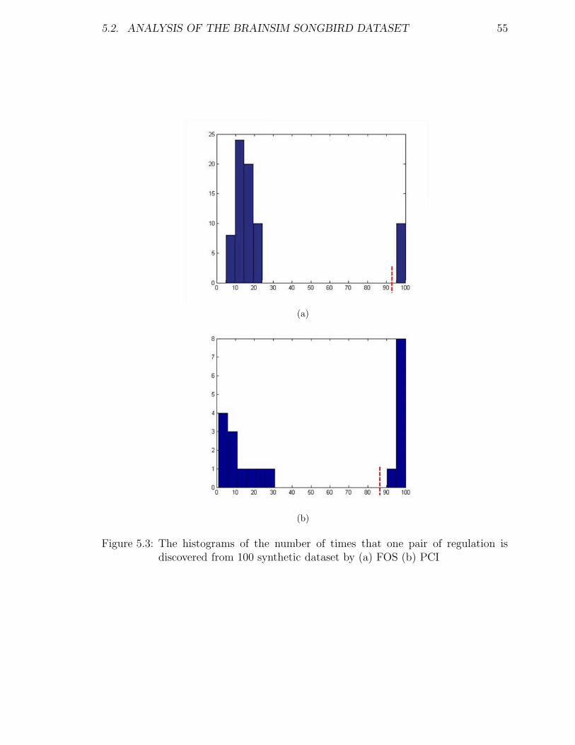
5.2. ANALYSIS OF THE BRAINSIM SONGBIRD DATASET 55
(a)
(b)
Figure 5.3: The histograms of the number of times that one pair of regulation isdiscovered from 100 synthetic dataset by (a) FOS (b) PCI

5.2. ANALYSIS OF THE BRAINSIM SONGBIRD DATASET 56
(a)
(b)
Figure 5.4: The final estimated networks of Synthetic Data by (a) FOS (b) PCI. Solidlinks are correctly discovered, TP; dashed links are missing ones, FN;

5.2. ANALYSIS OF THE BRAINSIM SONGBIRD DATASET 57
750 such Brainsim datasets as mentioned in Chapter 3. All the datasets have the same
underlying network structure. The network structure for 100 genes and one activity
term in each dataset is reverse engineered. Stopping criteria for FOS is set asK = 10.9
and the maximum number of regulators is 2, and for PCI, k = 1.5. Therefore,
similar to the previous section, 750 regulation weight matrices are generated for either
method, FOS and PCI.
5.2.1 Network Inference for Songbird data
To discover the significant regulations, all 750 regulation matrices reverse engineered
by FOS are summed. Note that for 100 genes there are more than 10k possible regu-
lations, and too many regulations that only appear one or twice out of 750 datasets,
therefore we only plot the histograms of the 50 most significant regulations, shown in
Figure 5.5. The threshold of 300 is used to select most significant regulations, which
should be comparable to the number of actual connections that is 11. By setting
the threshold, we have 11 significant regulations, which are used to build the final
network, shown in Figure 5.6.
For the implementation of PCI on Songbird Data, the histogram of the 50 most
significant regulations inferred out of 750 datasets is given in Figure 5.7. Due to the
criteria used to make the regulation weight matrix sparse, only a few regulations are
considered as significant ones. Therefore, most of insignificant regulations have been
removed and the histogram follows a more uniform distribution, and the threshold is
set as 600. This results in 10 significant regulations to build the network, shown in
Figure 5.8.
By comparing the inferred network by FOS Figure 5.6 with the original network

5.2. ANALYSIS OF THE BRAINSIM SONGBIRD DATASET 58
Figure 5.5: The histogram of topping 50 significant regulation discovered from 750Brainsim Songbird datasets by FOS.
Figure 5.6: The final estimated networks of Brainsim songbird Data using FOS.Dashed lines means the regulation that FOS could not recover.

5.2. ANALYSIS OF THE BRAINSIM SONGBIRD DATASET 59
Figure 5.7: The histogram of topping 50 significant regulation discovered from 750Brainsim Songbird datasets by PCI
Figure 5.8: The final estimated networks of Brainsim songbird Data using PCI.Dashed lines means the regulation that PCI could not recover.

5.2. ANALYSIS OF THE BRAINSIM SONGBIRD DATASET 60
structure Figure 3.3, it is observed that 10 out of all 11 inferred interactions are
truly captured and only one extra interaction is inferred: the regulation of Gene 5
by Activity. The co-regulation of Gene 6 by Gene 3 is missed by both methods,
which was either not predicted by previous studies of Brainsim Songbird Data [73];
because Gene 3 and Gene 5 control Gene 6 in a coordinated fashion with the lower
expression level of the pair serving as the limiting factor in the regulation of Gene 5, it
is found that Gene 5 had a lower expression level than Gene 3 in 89% of the temporal
cases, thus, Gene 5 nearly always serves as the effective regulator [73]. Analyzing the
inferred network through PCI Figure 5.8, 6 out of all 7 inferred interactions exist in
the actual network and 1 extra interaction from Gene 1 to Gene 5 is inferred. Five
interactions are missed. Both incorrectly inferred interaction using FOS and PCI is
the regulation of Gene 5. Both FOS and PCI are able to reverse engineer most of the
true regulations. To evaluate the accuracies of the obtained networks by FOS and
PCI, the criteria ‘precision’, ‘sensitivity’ and ‘specificity’ are calculated again, whose
results are shown in Table 5.4. As shown, FOS performed better than PCI with more
correctly detected regulations.
Fast Orthogonal Search Parallel Cascade Identification
Sensitivity 1011
= 91% 611
= 55%
Precision 1011
= 91% 67= 86%
Specificity 1008810089
≈ 100% 1008410089
≈ 100%
Table 5.4: Comparisons of the inferred networks of Brainsim Simulated Data by usingFOS and PCI

5.3. ANALYSIS OF YEAST SACCHAROMYCES CEREVISIAE DATASET 61
5.3 Analysis of Yeast Saccharomyces Cerevisiae
Dataset
A biological data consisting of 14 genes from yeast Saccharomyces cerevisiae [74],
including three time series, was ultimately used to evaluate the efficiency of these two
reverse engineering methods. The pathway of these genes in KEGG shown in Figure
3.4 is regarded as the target network used to compare and evaluate the performances
of FOS and PCI. Since CLN3 only works at the start of the cell cycle, we will not
consider its regulators for both methods, FOS and PCI. Stopping criteria used for
analyzing this data are the same as previous two datasets; for FOS is set as K = 10.9
and the maximum number of regulators is 2, and for PCI, k = 1.5. For this data, two
individual networks are inferred by the two methods.
5.3.1 Network Inference
As discussed in Chapter 3, the KEGG pathway is treated as the target network for
comparison. Complexes including one or several genes are considered as a ′gene′
in the network. There are 10 complexes, including CLN3/CDC28, SWI4/SWI6,
MBP1/SWI6, CLN1/CLN2/CDC18, and CLB5/CLB6/CDC28. Other nodes that
are made of one single gene only, CDC20, CDC6, SIC1, FAR1, and FUS. The follow-
ing assumptions are made:
• Genes CLN3 and CDC28 are only considered as possible regulators, as they
are starters of the cell cycle network.
• All discovered links from any gene in one complex to any other genes in a
different complex will be considered as one regulation. For example, if FOS or

5.3. ANALYSIS OF YEAST SACCHAROMYCES CEREVISIAE DATASET 62
PCI result in three regulations from the genes in the complex CLN3/CDC28 to
the genes in the complex SWI4/SWI6, CLN3 → SWI4, CLN3 → SWI6, and
CDC28 → SWI4, still only one regulation is used to construct the resulting
network. The weight of this regulation equals the maximum value of the weights
of these three regulations.
• All regulations among genes in the same complex will be ignored.
• If there exist two regulations between two complexes with different directions,
the weights of these regulations will be compared, and only the direction of one
regulation with the higher weight will be kept, which, therefore, determines the
directionality of regulation of these two complexes. For example, between a
complex cplxi and cplxj , if Rij and Rji are both nonzero and Rij > Rji, then
the directionality is determined as cplxi → cplxj . This interpretation is based
on the biological assumption that a small variation in the regulator gene will
result in a large change in the target gene.
The corresponding networks of the yeast dataset using FOS and PCI are shown
in Figure 5.9 (a) and (b). They are also compared with the two previous studies
[35, 85]. Details of their methods are not discussed here; instead, their results are
adopted for comparisons and their resulting networks are shown in Figure 5.9 (c) and
(d), respectively.
By comparing the inferred networks using FOS and PCI with the KEGG pathway,
it is observed that more than forty percent of the interactions in the target network
are inferred by FOS and PCI. While two interactions are captured by Kim et al. [35]
and three are captured by Zhang et al. [85]. Also, reverse engineered results using
FOS and PCI outperform the previous studies in terms of predicting more correctly

5.3. ANALYSIS OF YEAST SACCHAROMYCES CEREVISIAE DATASET 63
Figure 5.9: The yeast cell cycle pathway inferred from Spellman data using differentmethods: (a) FOS (b) PCI (c) Kim [35], and (d) Zhang [85].

5.3. ANALYSIS OF YEAST SACCHAROMYCES CEREVISIAE DATASET 64
estimated and misdirected interactions. Using the information from all four reverse
engineering approaches of cell cycle pathway of the yeast data, ‘precision’, ‘sensitivity’
and ‘specificity’ are calculated and displayed in Table 5.5, as a summary of Figure
5.9. Because different from synthetic dataset and songbird dataset, yeast dataset does
FOS PCI Kim[35] Zhang[85]
TPs 4 5 2 3
FPs 8 7 8 8
Sensitivity 40% 50% 20% 30%
Precision 29% 36% 15% 27%
Specificity 85% 85% 85% 86%
Table 5.5: Comparisons of the inferred networks of yeast Saccharomyces cerevisiaeData by using FOS, PCI and other two available studies.
not have replicate samples for analysis, its inferred results are less statistically sound
and hard to be evaluated. Even though, their absolute values are not very high, they
show significant improvement to the previously reported studies [35, 85].

Chapter 6
Summary and Conclusions
Reverse engineering gene regulatory networks from gene expression data is an im-
portant but challenging area of research in systems biology. In this thesis, Fast
Orthogonal Search and Parallel Cascade Identification, two system identification ap-
proaches, inspired by engineering systems, are introduced and employed to construct
GRNs using temporal gene expression data. The fast convergence time of FOS O(n2)
makes it an attractive approach to analyze large scale data. FOS searches all possible
regulator genes from a candidate set; it selects the optimal one, adds it to the model
and deletes it from the candidate set, iteratively. The selection procedure guarantees
that the searching will always select the most significant regulator from the exist-
ing possible regulators. The other approach, PCI, considers all possible regulators
simultaneously, but by assigning with different weights to them. A modification to
this algorithm was proposed to make the regulation weight matrix generated by PCI
sparse.
To evaluate the reliability and efficiency of FOS and PCI for inferring causal regu-
latory interactions from temporal gene expression data, a synthetic data is generated
65

CHAPTER 6. SUMMARY AND CONCLUSIONS 66
and used. FOS can recover 10 out of 11 actual regulations in this dataset, and PCI
using the proposed criteria can infer a sparse network and recover nine out of 11
true regulations. Via three statistical evaluation criteria ‘sensitivity’, ‘precision’ and
‘specificity’ as well as mean square error, the accuracies of the inferred structures
through both methods are quantified.
FOS and PCI are also applied to the Brainsim songbird data, a temporal simulated
dataset with known structure that models the singing behavior in a songbird. The
inferred structures quantified via the criteria ‘sensitivity’, ‘precision’ and ‘specificity’,
indicates a good performance of these two network inference approaches; only one out
of all inferred interactions is a false regulation using either approach, 10 true network
regulations can be recovered through FOS and six using PCI.
Finally the efficiencies of FOS and PCI for learning the network structure are
evaluated using a biological data, the temporal expression values of 14 genes in yeast
Saccharomyces cerevisiae cell cycle data reported in [74]. The networks inferred from
yeast data by FOS and PCI are compared to the KEGG pathway of the yeast as
the target network and two other yeast network inference studies on the same data
using evaluation criteria ‘sensitivity’, ‘precision’ and ‘specificity’. Even though, the
absolute values of these criteria are not high, compared with the two previous studies,
the results demonstrate a good performance of both FOS and PCI.
In conclusion, both FOS and PCI, can deal with continuous gene expression data,
capture their dynamics, and build deterministic models. By modeling the input/out
relationship, they can infer the causality of the gene regulatory networks by assigning
the input as the regulators of the output.

6.1. FURTHER DIRECTIONS 67
6.1 Further directions
Design and application of methods for reverse engineering of gene regulatory networks
from gene expression data, is a key aspect in systems biology. We proposed an idea
that can apply system identification algorithms well known for mathematics and
engineering into reverse engineering methods. A few future directions for this work
are listed below:
• Studying alternative basis functions to gene expression profile functions used as
the input in this work, to approximate the regression model of the association
between a given gene and that of its potential regulators in FOS and PCI.
• Considering biological knowledge to determine transcription factors or potential
gene regulators, assigning the gene expression functions of the potential genes
with higher probability to be selected as potential regulators. This can be done
by dividing the candidate functional set into several subsets; therefore, FOS
could start searching from the subset of a higher relevance and PCI can build
different groups of cascades by using different subsets.
• Generalizing the proposed model to a model that allows different regulators
of a gene regulate their target gene with different time lags, instead of 1 time
lag assumption used in this work. This can result in a more flexible network
inference model with higher accuracy.
• Incorporating biological information to determine the maximum number of po-
tential gene regulators for a given gene, instead of defining equal maximal num-
ber of regulators for all genes. Since FOS always selects regulators for a given
target gene, this prior knowledge can make an improvement.

6.1. FURTHER DIRECTIONS 68
• Because Parallel Cascade Identification randomly assigns coefficients to the in-
put in the dynamic system, applications of alternative algorithms used to gen-
erate the impulse response might decrease the computation time of PCI model.
• Further studying possible approaches for defining the significance of a regulation
in the regulation weight matrix generated by PCI.

Bibliography
[1] Cell cycle: yeast saccharomyces cerevisiae. http : //www.genome.jp/dbget −bin/wwwbget/map04111.
[2] T. Akutsu, S. Miyano, and S. Kuhara. Identification of genetic networks from a
small number of gene expression patterns under the boolean network model. in
Proceedings of Pacific Symposium on Biocomputing, 4:17–28, 1999.
[3] A. A. Alizadeh, M. B. Eisen, R. E. Davis, C. Ma, and etc. Distinct types of
diffuse large b-cell lymphoma identified by gene expression profiling. Nature,
403:503–511, 2000.
[4] M. Bansal, G. D. Gatta, and D. di Bernardo. Inference of gene regulatory
networks and compound mode of action from time course gene expression profiles.
Bioinformatics, 22(7):815–822, 2006.
[5] K. Basso, A. A. Margolin, G. Stolovitzky, U. Klein, R. D. Favera, and A. Califano.
Reverse engineering of regulatory networks in human b cells. Nature Genetics,
37(4):382–390, 2005.
[6] S. Bornholdt. Boolean network models of cellular regulation: prospects and
limitations. Journal of the Royal Society, 5(Suppl 1):85–94, 2008.
69

BIBLIOGRAPHY 70
[7] L. Campos and J. Huete. On the use of independence relationships for learn-
ing simplified belief networks. International Journal of Intelligent Systems,
12(7):495–522, 1998.
[8] T. Chen, H. L. He, and G. M. Church. Modeling gene expression with differen-
til equations. in Proceedings of Pacific Sympposium on Biocomputing, 4:29–40,
1999.
[9] X. Chen, G. Anantha, and X. Wang. An effective structure learning method for
constrcting gene networks. Bioinformatics, 22(11):1367–1374, 2006.
[10] A. Crombach and P. Hogeweg. Evolution of evolvability in gene regulatory net-
works. PLoS Computational Biology, 4(7):e1000112, 2007.
[11] X. Cui and G. A. Churchill. Statistical tests for differential expression in cDNA
microarray experiments. Genome Biology, 4(4):210.1–210.10, 2003.
[12] M. S. Dasika, A. Gupta, and C. D. Maranas. A mixed integer linear programming
framework for inferring time delay in gene regulatory networks. in Proceedings
of Pacific Symposium on Biocomputing, 9:474–485, 2004.
[13] E. H. Davidson and D. H. Erwin. Gene regulatory networks and the evolution
of animal body plans. Science, 311(5762):796–800, 2006.
[14] A. G. de Brevern, S. Hazout, and A. Malpertuy. Influence of microarrays exper-
iments missing values on the stability of gene groups by hierarchical clustering.
BMC Bioinformatics, 5:114–225, 2004.
[15] M. J. L. de Hoon, S. Imoto, K. Kobayashi, N. Ogasawara, and S. Miyano. Infer-
ring gene regulatory networks from time-ordered gene expression data of bacillus

BIBLIOGRAPHY 71
subtilis using differential equations. in Proceedings of Pacific Symposium on
Biocomputing, 8:17–28, 2003.
[16] A. A. Desrochers. On an improved model reduction technique for nonlinear
systems. Automatica, 17(2):407–409, 1981.
[17] P. D’haeseleer, S. Liang, and R. Somogyi. Genetic network inference: from
co-expression clustering to reverse engineering. Bioinformatics, 16(8):707–762,
2000.
[18] P. D’haeseleer, X. Wen, S. Fuheman, and R. Somogyi. Linear modeling of mrna
expression levels during cns development and injury. in Proceedings of the 4th
Pacific Symposium on Biocomputing, 4:41–52, 1999.
[19] P. D’haeseleer, X. Wen, S. Fuhrman, and R. Somogyi. Mining the gene expression
matrix: Inferring gene relationships from large scale gene expression data. in
Proceedings of the second international workshop on Information Processing in
Cells and Tissues, pages 203–212, 1998.
[20] S. Draghici. Data Analysis tools for DNA microarrays. Chapman and Hall-CRC,
2003.
[21] N. Friedman. Learning bayesian network structure from massive datasets: the
sparse candidate algorithm. in Proceedings of Fifteenth Conference on Uncer-
tainty in Artificial Intelligence, pages 206–215, 1999.
[22] N. Friedman, M. Linia, I. Nachman, and D. Pe’er. Using bayesian networks to
analyze expression data. Journal of Computation Biology, 7(3):601–620, 2000.

BIBLIOGRAPHY 72
[23] T. S. Gardner and J. J. Faith. Reverse engineering transcription control networks.
Physics of Life Reviews, 2(1):65–88, 2005.
[24] D. Heckerman, D. Geiger, and D. Chickering. Learning bayesian networks: the
combination of knowledge and statistical data. Machine Learning, 20(3):197–243,
1995.
[25] J. Herrero, R. Diaz-Urizrte, and J. Dopazo. Gene expression data preprocessing.
Bioinformatics, 19(5):655–656, 2003.
[26] S. Huang. Gene expression profiling, genetic networks, and cellular states: an
integrating concept for tumorigenesis and drug discovery. Journal of Molecular
Medicine, 77(6):469–480, 1999.
[27] T. Ideker, V. Thorsson, A. F. Siegel, and L. E. Hood. Testing for differentially
expressed genes by maximum likelihood analysis of microarray data. Journal of
Computational Biology, 7(6):805–817, 2000.
[28] R. Kabli, F. Herrmann, and J. McCall. A chain model genetic algorithm for
bayesian network structure learning. in Proceedings of the 9th annual conference
on Genetic and evolutionary computation, pages 1264–1271, 2007.
[29] G. Karlebach and R. Shamir. Modelling and analysis of gene regulatory networks.
Nature Reviews Molecular Cell Biology, 9(10):770–780, 2008.
[30] S. A. Kauffman. Homeostasis and differentiation in random genetic control net-
works. Nature, 224:177–178, 1969.
[31] S. A. Kauffman. Metabolic stability and epigenesis in randomly constucted ge-
netic nets. Journal of Theoretical Biology, 22(3):437–467, 1969.

BIBLIOGRAPHY 73
[32] S. A. Kauffman. The large scale structure and dynamics of genetic control cir-
cuits: an ensemble approach. Journal of Theoretical Biology, 44(1):167–190,
1974.
[33] S. A. Kauffman and L. Glass. The logical analysis of continuous, nonlinear
biochemical control networks. Journal of Theoretical Biology, 39(1):103–129,
1973.
[34] H. Kim, G. H. Golub, and H. Park. Missing value estimation for DNA microarray
gene expression data: local least squares imputation. Bioinformatics, 21(2):187–
198, 2006.
[35] S. Y Kim, S. Imoto, and Miyano S. Inferring gene networks from time series
microarray data using dynamic bayesian networks. Briefings in bioinformatics,
4(3):228–235, 2003.
[36] M. J. Korenberg. Orthogonal identification of nonlinear difference equation mod-
els. in Proceedings of 28th Midwest Symposium on Circuits and Systems, 1:90–95,
1985.
[37] M. J. Korenberg. Fast orthogonal identification of nonlinear difference equation
and function expansion models. in Proceedings of 30th Midwest Symposium on
Circuits and Systems, 1:270–276, 1987.
[38] M. J. Korenberg. A robust orthogonal algorithm for system identification and
time-series analysis. Biological Cybernetics, 60(4):267–276, 1989.
[39] M. J. Korenberg. Parallel cascade identification and kernel estimation for non-
linear systems. Annals of Biomedical Engineering, 19(4):429–455, 1991.

BIBLIOGRAPHY 74
[40] M. J. Korenberg. Prediction of treatment response using gene expression profiles.
Journal of Proteome research, 1(1):55–61, 2002.
[41] M. J. Korenberg. On predicting medulloblastoma metastasis by gene expression
profiling. Journal of Proteome Research, 3(1):91–96, 2004.
[42] M. J. Korenberg, C. J. H. Brenan, and I. W. Hunter. Raman spectral estimation
via fast orthogonal search. Analyst, 122:879–882, 1997.
[43] M. J. Korenberg, R. David, I. W. Hunter, and J. E. Solomon. Parallel cas-
cade identification and its application to protein family prediction. Journal of
Biotechnology, 91(1):35–47, 2001.
[44] M. J. Korenberg and I. W. Hunter. Rapid dtmf signal classification via parallel
cascade identification. Electronics Letters, 32:1862–1863, 1996.
[45] M. J. Korenberg and L. D. Paarmann. Orthogonal approaches to time-series
analysis and system identification. IEEE Signal Processing Magazine, 8(3):29–
43, 1991.
[46] M. J. Korenberg, J. E. Solomon, and M. E. Regelson. Parallel cascade iden-
tification as a means for automatically classifying protein sequences into struc-
ture/function groups. Biological cybernetics, 82(1):15–21, 2000.
[47] S. Lang. Real and functional analysis. Transactions of the American Mathemat-
ical Society, 41(3):88–89, 1937.
[48] R. D. Leclerc. Survival of the sparsest: robust gene networks are parsimonious.
Molecular systems biology, 4(213):1–6, 2008.

BIBLIOGRAPHY 75
[49] P. Leray and O. Francois. Bayesian network structural learning and incomplete
data. in Proceedings of the international and interdisciplinary conference on
adaptive knowledge representation and reasoning, pages 33–40, 2005.
[50] S. Liang, S. Fuhrman, and R. Somogyi. Reveal, a general reverse engineering
algorithm for inference of genetic network architectures. in Proceedings of Pacific
Symposium on Biocomputing, 3:18–29, 1998.
[51] W. K. Lim, K. Wang, C. Lefebvre, and A. Califano. Comparative analysis of mi-
croarray normalization procedures: effects on reverse engineering gene networks.
Bioinformatics, 23(13):282–288, 2007.
[52] D. R. McGaughey, M. Tarbouchi, K. Nutt, and A. Chikhani. Speed sensorless
estimation ac induction motors using the fast orthogonal search algorithm. IEEE
Transactions on Industry Applications, 21(1):112–120, 2006.
[53] C. B. Moler. Numerical computing with MATLAB. Philadelphia: Society for
Industrial and Applied Mathematics, 2004.
[54] S. Mostafavi, S. Baranzini, J. Oksenberg, and P. Mousavi. A fast multivari-
ate feature-selection/classification approach for prediction of therapy in multiple
sclerosis. in Proceedings of IEEE Conference on Computational Intelligence in
Bioinformatics and Computational Biology, pages 1–8, 2006.
[55] K. Mountjoy, E. Morin, and K. Hashtrudi-Zaad. Use of the fast orthogonal search
method to estimate optimal joint angle for upper limb hill-muscle models. IEEE
Transactions on Biomedical Engineering, 57(4):790–798, 2010.

BIBLIOGRAPHY 76
[56] D. M. Mutch, A. Berger, R. Mansourian, A. Rytz, and M. Roberts. The limit fold
change model: a practical approach for selecting differentially expressed genes
from microarray data. BMC Bioinformatics, 3(17), 2002.
[57] H. G. Natke. Application of system identification in Engineering. Springer, New
York, 1988.
[58] R. E. Neapolitan. Learning Bayesian networks (artificial intelligence). New York:
Prentice–Hall, 2004.
[59] S. Oba, M. A. Sato, I. Takemasa, M. Monden, K. I. Matsubara, and S. Ishii.
A bayesian missing value estimation method for gene espression profile data.
Bioinformatics, 19(16):2088–2096, 2000.
[60] H. Ogata, S. Goto, W. Fujibuchi, and M. Kanehisa. Computation with the kegg
pathway database. Biosystems, 47(1-2):119–128, 1998.
[61] S. F. Orfanidis. Optimum signal processing. McGraw-Hill, New York, 1988.
[62] B. E. Perrin, L. Ralaivola, A. Mazurie, S. Bottani, J. Mallet, and F. d’Alche
Buc. Gene networks inference using dynamic bayesian networks. Bioinformatics,
19(Suppl 2):ii138–148, 2003.
[63] M. Pineda-Sanchez, M. Riera-Guasp, J. A. Antonino-Daviu, J. Roger-Folch,
J. Perez-Cruz, and R. Puche-Panadero. Instantaneous frequency of the left side-
band harmonic during the start-up transient: A new method for diagnosis of
broken bars. IEEE Transactions on Industrial Electronics, 56(11):4557–4570,
2009.

BIBLIOGRAPHY 77
[64] L. Qian, H. Wang, and E. R. Dougherty. Inference of noisy nonlinear differ-
ential equation models for gene regulatory network using genetic programming
and kalman filtering. IEEE Transactions on Signal Processing, 56(7):3327–3339,
2008.
[65] T. M. Rakoczy. Feature selection for computer-aided diagnosis of breast cancer
using dynamic contrast-enhanced magnetic resonance images. Master’s thesis,
Royal Military College of Canada, September 2009.
[66] J. C. Rapp, B. J. Baumgartner, and J. Mullet. Quantitative analysis of tran-
scription and rna levels of 15 barley chloroplast genes. The Journal of Biological
Chemistry, 267(30):21404–21411, 1992.
[67] W. Richard. Genes and DNA. Kingfisher, Boston, 2003.
[68] H. E. Samad, M Khammash, L. Petzold, and D. Gillespie. Stochastic modeling
of gene regulatory networks. International Journal of Robust Nonlinear Control,
15:691–711, 2005.
[69] M. Schena, D. Shalon, R. W. Davis, and P. O. Brown. Quantitative monitoring
of gene expression patterns with a complementary DNA microarray. Science,
270(5235):467–470, 1995.
[70] A. Schulze and J. Downward. Navigating gene expression using microarrays: a
technology review. Nature cell biology, 3(8):E190–E195, 2001.
[71] J. Shao. Mathemtical Statistics. Springer, New York, 2005.
[72] C. Sima, J. Hua, and S. Jung. Inference of gene regulatory networks using time-
series data: A survey. Current Genomics, 10(6):416–429, 2009.

BIBLIOGRAPHY 78
[73] V. A. Smith, E. D. Jarvis, A. J. Hartemink, and E. J. Hartemink. Evaluating
functional network inference using simulations of complex biological systems.
Bioinformatics, 18(Suppl 1):S216–S224, 2002.
[74] P. T. Spellman, G. Sherlock, M. Q. Zhang, V. R. Iyer, K. Anders, M. B. Eisen,
P. O. Brown, D. Botstein, and B. Futcher. Comprehensive identification of
cell cycle-regulated genes of the yeast saccharomyces cerevisiae by microarray
hybridization. Molecular Biology of the Cell, 9(12):3273–3297, 1998.
[75] P. Spirtes, C. Glymour, and R. Scheines. Causation, Prediction and Search. MIT
Press, 2001.
[76] N. Sugimoto and H. Iba. Inference of gene regulatory networks by means of
dynamic differential bayesian networks and nonparametric regression. Genome
Informatics, 15(2):121–30, 2004.
[77] O. Troyanskaya, M. Cantor, G. Sherlock, P. Brown, T. Hastie, R. Tibshirani,
D. Botstein, and R. B. Altman. Missing value estimation methods for DNA
microarrays. Bioinformatics, 17(6):520–525, 2001.
[78] E. P. van Someren, L. F. Wessels, E. Backer, and M. L. Reinders. Genetic
network modeling. Pharmacogenomics, 3(4):507–25, 2002.
[79] E. P. van Someren, L. F. Wessels, and M. L. Reinders. Linear modeling of genetic
networks from experimental data. in Proceedings of International Conference on
Intelligent Systems for Molecular Biology, 8:355–66, 2000.

BIBLIOGRAPHY 79
[80] X. Wang, A. Li, Z. Jiang, and H. Feng. Missing value estimation for DNA
microarray gene expression data by support vector regression imputation and
orthogonal coding scheme. BMC Bioinformatics, 7(32), 2006.
[81] D. C. Weaver, C. T. Workman, and G. D. Stormo. Modeling regulatory networks
with weight matrices. in Proceedings of the Pacific Symposium on Biocomputing,
4:112–123, 1999.
[82] R. F. Weaver. Molecular Biology. McGraw Hill, 2008.
[83] M. K. Yeung, J. Tegner, and J. J. Collins. Reverse engineering gene networks
using singular value decomposition and robust regression. Proceedings of the
National Academy of Sciences of the United States of America, 99(9):6163–6168,
2002.
[84] J. Yu, V. A. Smith, P. P. Wang, A. J. Hartemink, and E. D. Jarvis. Using
bayesian network inference algorithms to recover molecular genetic regulatory
networks. in Proceedings of third International Conference on System Biology,
37(382–390), 2002.
[85] Y. Zhang, Z. Deng, H. Jiang, and P. Jia. Inferring gene regulatory networks
from multiple data sources via a dynamic bayesian network with structural EM.
Lecture Notes in Computer Science, 4544:204–214, 2007.