A—1

Table of Contents APPENDIX A: PHYSICAL PLATFORM AND OPTICAL DESIGN ............ A—1

A.1 OPTICAL PATH .............................................................................................. A—1 A.2 MEASUREMENT CUVETTE AND POSITION CONTROL SYSTEM........................ A—4 A.3 FLUID TRANSFER CONTROL SYSTEM............................................................. A—6 A.4 TISSUE SIMULATOR FOR USE IN NIV INSTRUMENT....................................... A—7 A.5 CALCULATION OF EXPECTED POWER ............................................................ A—9

APPENDIX B: SOFTWARE DESIGN............................................................... B—1 B.1 SOFTWARE SYSTEM STRUCTURE................................................................... B—1 B.2 UREA MONITORING SYSTEM GRAPHICAL USER INTERFACE ....................... B—15

APPENDIX C: DIALYSIS EFFICIENCY MONITOR HARDWARE DESIGN C—1

C.1 HARDWARE MODULES .................................................................................. C—1 C.2 SPECIFICS OF DEM HARDWARE DESIGN....................................................... C—2

APPENDIX D: INTERFERING SUBSTANCE ABSORBANCE TABLE ..... D—1

APPENDIX E: HUMAN SUBJECTS STUDY PROTOCOL........................... E—1

APPENDIX F: ACOUSTO-OPTICAL TUNABLE FILTERS.........................F—1

A—2

Table of Figures Figure A.1.1: The Optical mounting channel is fabricated from aluminum. ............................................ A—2 Figure A.1.2: Side view of the spacing of optical components used to fulfill the AOTF light input requirements ............................................................................................................................................. A—3 Figure A.2.1: Lens mount 2 ...................................................................................................................... A—4 Figure A.2.2: The measurement fluid is contained in a Teflon bag.......................................................... A—5 Figure A.2.3: The measurement cuvette has two chambers, each of which contains a teflon bag ........... A—5 Figure A.2.4: The Position Control System mounting hardware is coupled to the measurement cuvette by a precision lead screw ................................................................................................................................. A—6 Figure A.3.1: The measurement fluids are delivered to the measurement cuvette by the fluid control system, which consists of a pump and solenoid valves .......................................................................................... A—7 Figure A.4.1: Dimensions of the measurement head of the NIV Prototype. ............................................. A—8 Figure A.4.2: Transmission of two layers of 0.01" silicon membrane...................................................... A—8 Figure A.4.3: Assembly drawing of the measurement cuvette. ................................................................. A—9 Figure A.5.1: Power Spectrum for a halogen lamp being operated at 3000 K....................................... A—11 Figure B.1.1: Urea Monitoring System Software block diagram. ............................................................ B—2 Figure B.1.2: Flowchart of the Idle Loop Control Software. ................................................................... B—3 Figure B.1.3: Flowchart of a urea measurement cycle............................................................................. B—6 Figure B.1.4: Flowchart of the intensity balancing process algorithm. ................................................... B—7 Figure B.1.5: Control word format for the 12 bit converter................................................................... B—13 Figure B.2.1: The main user interface window for the UMS software system........................................ B—18 Figure B.2.2: The system spectrum window from the UMS system software.......................................... B—19 Figure B.2.3: The Stray Light Optimization Window from the UMS system software............................ B—20 Figure B.2.4: The noise performance/bias cancellation window from the UMS system software.......... B—20 Figure B.2.5: The menu bar and File pull down menu from the UMS system software. ........................ B—21 Figure B.2.6: The menu bar and Start Acquisition pull down menu from the UMS system software..... B—21 Figure B.2.7: The menu bar and Calibration pull down menu from the UMS system software. ............ B—21 Figure B.2.8: The menu bar and Spectrum Analysis pull down menu from the UMS system software. . B—21 Figure B.2.9: The menu bar and Noise Analysis pull down menu from the UMS system software. ....... B—22 Figure C.1.1:Block diagram of the DEM system hardware shows there are two main interfaces to the PC...................................................................................................................................................................C—2 Figure C.2.1:Responsivity curve of an InGaAs photodetector .................................................................C—5 Figure F.1.1:Setup of typical AO diffraction system ................................................................................ F—1

A—1

APPENDIX A: PHYSICAL PLATFORM AND OPTICAL DESIGN

In any optical system, it is important to properly focus and deliver light to the sample. In this chapter, we will describe the optical design and physical layout of the urea monitoring system. There are several concerns that must be addressed in the physical design of this system. These include: • = How the dialysis fluid is to be transferred to the sample compartment. • = The design of the measurement cuvette. • = The optical layout of the system, including compartments and mounting hardware. • = The design of the position control system. Many of these issues have been the subject of a separate research project done by Jamie Murdock at WPI. Mr. Murdock’s Master’s Thesis involves the design of a measurement cuvette for a general analyte monitor that utilizes the Optical Bridge principle. Mr. Murdock designed the position control system, fluid delivery system and the measurement cuvette. He also designed a first generation prototype of the optical layout during an earlier research project. This design has been reworked into a more compact prototype. We shall now describe the current prototype design in the context of how it implements the Optical Bridge principle. The overall optical system design in shown in Figure A.1.1.

A.1 Optical Path The system design requires that the light must be focused at two places: the input to the AOTF and at the sample. Two major optical assemblies are used to accomplish this task. A set of two plano-convex (PCX) lenses are used as a condensing lens to focus the light into the input aperture of the AOTF. Following the condensing lenses are an Infrared sheet film polarizer (Polaroid Corp.) and a circular aperture. These components are contained in the block labeled “Lens and Polarizer Holder #1” in Figure A.1.1. These components are used to fill the AOTF operating parameters. These operating parameters state that light entering the AOTF must be polarized, and be at a maximum angle of 3.5° from normal. After the AOTF, another set of condensing lenses are mounted in order to focus light onto the sample. A second polarizer, rotated 90° from the first, is used to cut out the stray light from the beam. This reduces the amount of the zeroth order beam from the AOTF that enters the sample, since the zeroth order beam is unpolarized. A beam cutter made from a piece of 1/8” brass is also placed in the path to further block the zero order beam. This beam cutter can be moved in and out in order to optimize the blockage. After the condensing lenses, a beam splitter made from a piece of glass is mounted at a 45° angle to the beam. In Figure A.1.1, these components are contained in the block labeled “Lens and Polarizer Holder #2”. The splitter directs about 8% of the incident light to the Input Light Detector (ILD). The detector is therefore able to record how much light is transmitted to the entrance of the sample. The rest of the light then passes straight through the sample, and hits the Sample Light Detector (SLD).

A—2

A.1.1 Mounting Hardware All of the optical components required to focus, tune, and deliver the light to the sample are mounted on an aluminum channel. Bert Kupcinskas of A.K. Machine Co., Inc., (Millbury, MA) donated time, materials and expertise to the design of this channel and the mounting components. This channel is U-shaped with an outer width of 3” and an inner width of 2”. The channel is ¼” deep, and the overall height of the piece is 1 ½”. This channel is mounted on a 4” tall base enclosure which contains electronic connections and is enclosed by a 4” tall aluminum sheet metal cover to block ambient light. Figure A.1.1 shows an isometric drawing of the channel and the mounting components.

Figure A.1.1: The Optical mounting channel is fabricated from aluminum. The mounting components are, from left to right, the lamp and holder, condensing lens holder 1, AOTF mounting block and AOTF, condensing lens holder 2 and beam splitter, and the measurement cuvette. The baffle has been omitted for clarity. Figure adapted from [77].

A.1.2 Optical Components The light source for this system is a 100W halogen lamp. The light source is mounted on a holding base. The holding base is mounted inside a 1 ¼” circular pocket that is approximately ¼” deep. A 3/8” diameter through hole is drilled at the center of this pocket for the lamp power wires to pass through. The center of the lamp mounting pocket is located 1 ½” from the end of the channel. The lamp is enclosed by a baffle, which is made of a sheet of 1/8” thick aluminum that has been bent into an L-shape. The baffle has a ¾” diameter hole that allows light to enter the lens assembly. The baffle is used to prevent unwanted light from entering the rest of the optical system. The light is then coupled into the rest of the system, where the control of wavelength and intensity is accomplished. Please note that dimensions of machined parts are given in inches due to

A—3

machinist’s conventions, while many of the dimensions for the optical components are given in mm, due to optical conventions. Wavelength and intensity control of the light that hits the sample is accomplished using an Acousto-Optical Tunable Filter (AOTF – See Appendix F). As stated earlier in this section, there are three requirements for the light that enters the AOTF. First, the light must be polarized. Second, the light should be focused on the input of the AOTF. Finally, the AOTF has a maximum acceptance angle of 7º, which means that light entering the device can deviate no more that 3.5º from the normal. In order to fill these requirements, several components are inserted into the optical path. The first is a set of condensing lenses. These lenses have focal lengths of 50mm and diameters of 25mm. The second is an aperture, which has an inner diameter of 9mm. The final component is a sheet of infrared polarizing filter film. All of these components are mounted in a Delrin block. The relative placement of the components is shown in Figure A.1.2. The mounting block is composed of two sections, each of which has a ¾” diameter hole drilled in the center. The mounting block is 1 ½” long, 2” wide, and 1 ¾” high. The first section is ½” long. A 1” square pocket is milled into the inside of this piece to hold the polarizing film. The pocket is 0.003” deep. This piece is mated to the other section with four screws. The second section has a 1” diameter hole drilled 0.456” into the center. The condensing lenses are inserted into this hole, separated by a rubber O-ring.

Figure A.1.2: Side view of the spacing of optical components used to fulfill the AOTF light input requirements. Figure adapted from [77].

At the bottom of the hole is the aperture, which is a made from a 1/16” thick ring of Mercarto. The leading edge of the mounting block is mounted 3 1/8” from the end of the channel. Refer to Figure A.1.1 for the location of the mounting block in the optical path. One the left is the piece that holds the aperture, lenses, and O-rings. On the right is the mating piece, showing the pocket that holds the polarizer. The AOTF mounting platform is a ½” thick aluminum block. The block is 2” square. It is located 5.5” from the end of the channel. The AOTF is mounted directly onto this block with four screws. The block is slotted to allow lateral movement for system optimization. Figure A.1.1 shows the location of this mounting block and the AOTF in the optical path. The second set of focusing lenses are contained in a larger mounting block assembly. This mounting block consists of three pieces. The first piece is similar

A—4

to the polarizer holder that is part of the first lens mounting. The second piece is a lens holder, again similar to the lens holder of the first mounting block. The lens assembly in this block is slightly different. The first lens is similar to those in the other block, having a diameter of 25mm and a focal length of 50mm. The second lens has a diameter of 25 mm and a focal length of 100mm. This gives some magnification to the system. These lenses are also mounted 1.1mm apart. They are separated by two O-rings, since the 100 mm f.l. lens is thicker. This block has a 45° cut on back side. The front side of this block also has a pocket milled into the face. This pocket is 0.003” deep and is meant to hold the beam cutter. The beam cutter is fabricated from a piece of 1” x 1 ½” x 1/8” brass. The brass has been painted with a flat black paint to reduce light reflectance. The beam cutter slides into and out of the optical path in order to remove the zeroth order beam, which is split off to the left of the desired first order beam. The third piece mates to this cut. The third piece also has a 45° face, but it has a pocket milled into the face. This pocket, which is 1/8” thick, holds a piece of glass that acts as a beam splitter. This block has a ¾” hole drilled through it to complete the light path. A second ¾” inch hole is drilled at right angles to the first that leads from the beam splitter. The Input Light Detector is mounted into this hole. The straight path leads to the measurement cuvette. Figure A.2.1 shows the three-piece lens mount assembly. Please refer back to Figure A.1.1 to see the relative placement of this mounting block. The leading edge of the mounting block is 7 7/8” from the end of the channel.

A.2 Measurement Cuvette and Position Control System In the description of the Optical Bridge that has been given in the previous chapters, it was stated that the balancing stage of the measurement was done with only the clean dialysate in the optical path. It is also necessary to change the pathlength through this sample. The measurement stage of the reading is performed with both the clean and spent dialysate solutions in the optical path. It was necessary to find a way to implement these requirements.

Figure A.2.1: Lens mount 2. The piece on the left mates to the middle piece and has a pocket to hold a sheet of polarizing film. The middle piece mates to the beam splitter holder and contains the second set of lenses and O-rings. The piece on the right holds the beam splitter and has two through holes at right angles to each other. The input light detector is attached to the top through one hole, and the measurement cuvette is placed on the right hand side. (The holes are on the right and top of the figure. )

A special measurement cuvette was designed to fulfill these requirements. The measurement cuvette has two compartments. The cuvette itself is manufactured from a block of Delrin. It has two drainage holes in the bottom, and a keyway that holds a moveable piece of 1/8” thick acrylic. At the front of the cuvette, a piece of ¼” thick acrylic is attached. A slider made from another Delrin block fits into the keyway cut into the back face. The Sample Light Detector is mounted inside this slider. The thin acrylic

A—5

piece floats in the center of the cuvette, and is held in place by two leaf springs made from ¼” thick spring steel. This forms a two-chamber cuvette. A clear bag made of Teflon is placed in each chamber. The Teflon bag is shown in Figure A.2.2. The bag closest to the front face contains the clean dialysate. The second bag contains the spent dialysate. During the balancing stage of the measurement, the slider is moved into the cuvette, and it displaces the spent fluid from the bag, leaving only the clean dialysis fluid in the optical path. When the measurement stage begins, the slider moves out of the compartment, which allows the spent fluid back into the bag, and therefore into the optical path. Figure A.2.3 is an isometric drawing of the measurement cuvette.

Figure A.2.2: The measurement fluid is contained in a Teflon bag. Figure adapted from [77].

Figure A.2.3: The measurement cuvette has two chambers, each of which contains a teflon bag (not shown.) A slider moves in and out of the cuvette to change the pathlength and occlude the spent dialysate from the optical path. Figure adapted from [77].

The movements of the slider are generated by a stepper motor (Airpax) that is coupled to the slider. The stepper motor has a resolution of 200 steps per revolution of the motor shaft. It is coupled to a precision lead screw (Edmund Scientific) that has a pitch of 1 thread per mm, for an overall resolution of approximately 5 µm per step. The movement of the motor are generated by the PC and sent from the digital board. See Chapter Appendix B: for a complete description of the software required to control the stepper motor. The motor assembly is shown in Figure A.2.4.

A—6

Figure A.2.4: The Position Control System mounting hardware is coupled to the measurement cuvette by a precision lead screw. Figure adapted from [77].

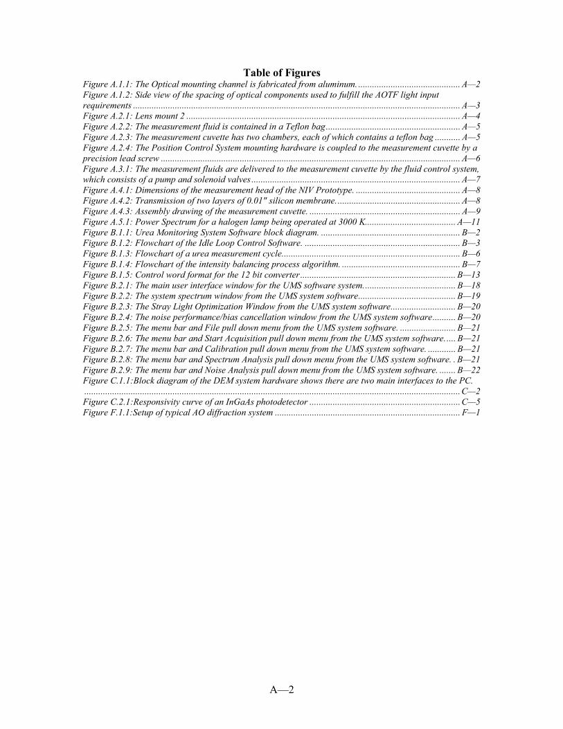
A.3 Fluid Transfer Control System The fluid control transfer system consists of a peristaltic pump, tubing set, heater, and temperature controller. The pump, under control from the PC, transfers equal amounts of the clean and spent dialysate, approximately 10 ml, to each of the Teflon measurement bags. At the end of the measurement, approximately 30 ml of each fluid is pumped through the system in order to reduce sample carryover. This is currently done under manual control by the user, but could be automated in future designs. The fluid is delivered through 18 inches of Masterflex™ tubing. The tubing is wrapped with heating tape, and is kept at 37° C through the use of a commercial heat controller (Omega Inc.) The tubing is connected to the measurement bags through the use of 4 way luer lock adapters. The side entrances of the luer adapter are fitted with specially modified caps that contain either a thermistor or a T-type thermocouple. The thermocouple is used as an input to the temperature controller, while the thermistor is used to give temperature information to the software to be used in the urea concentration algorithm.

A—7

Figure A.3.1: The measurement fluids are delivered to the measurement cuvette by the fluid control system, which consists of a pump and solenoid valves. The temperature of the fluids are carefully controlled by the heating unit and the heating tape. Figure adapted from [77].

This pump and temperature control system has been designed by Jamie Murdock as a part of his Master’s thesis. The hardware and software for controlling the pump and solenoid valves are given in Appendix B and C. The overall system is represented in Figure A.3.1.

A.4 Tissue Simulator for Use in NIV Instrument As stated in Chapters 2 and 3, we intend to compare the performance of the instrument designed for this research with the NIV instrument. It was therefore necessary to design and build a measurement cuvette that would fit into that instrument. The term tissue simulator is used to mean a two compartment cuvette This presented somewhat of a practical challenge, as that instrument was designed to measure a human earlobe rather than an aqueous sample. The cuvette had the following design requirements:

• = Two compartments, one of which contains the sample and the other contains the background fluid

• = The sample compartment must be completely compressible • = The background fluid compartment must be slightly compressible • = The cuvette must transmit adequate amounts of light • = The cuvette must provide a measure of temperature stability

MeasurementCuvette

Heating Tape

Temp Control Unit

Peristaltic Pump w/ inlet Solenoid

Inlet forbackground

Outlet

Inlet for Spent

To Drain

Heating tape control leads

Filtered light from optical system

A—8

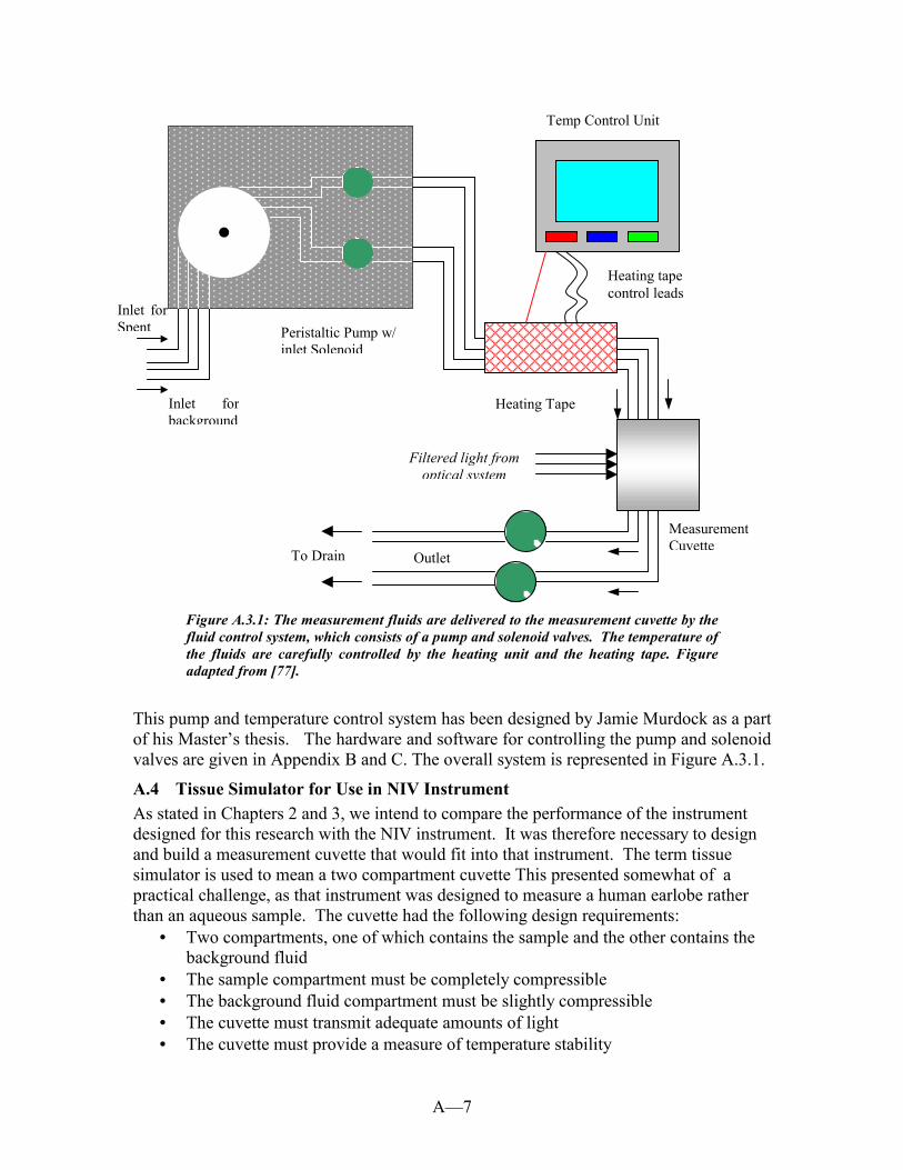
• = The cuvette must fit into the measurement head of the NIV instrument, shown below in Figure A.4.1.

Figure A.4.1: Dimensions of the measurement head of the NIV Prototype.

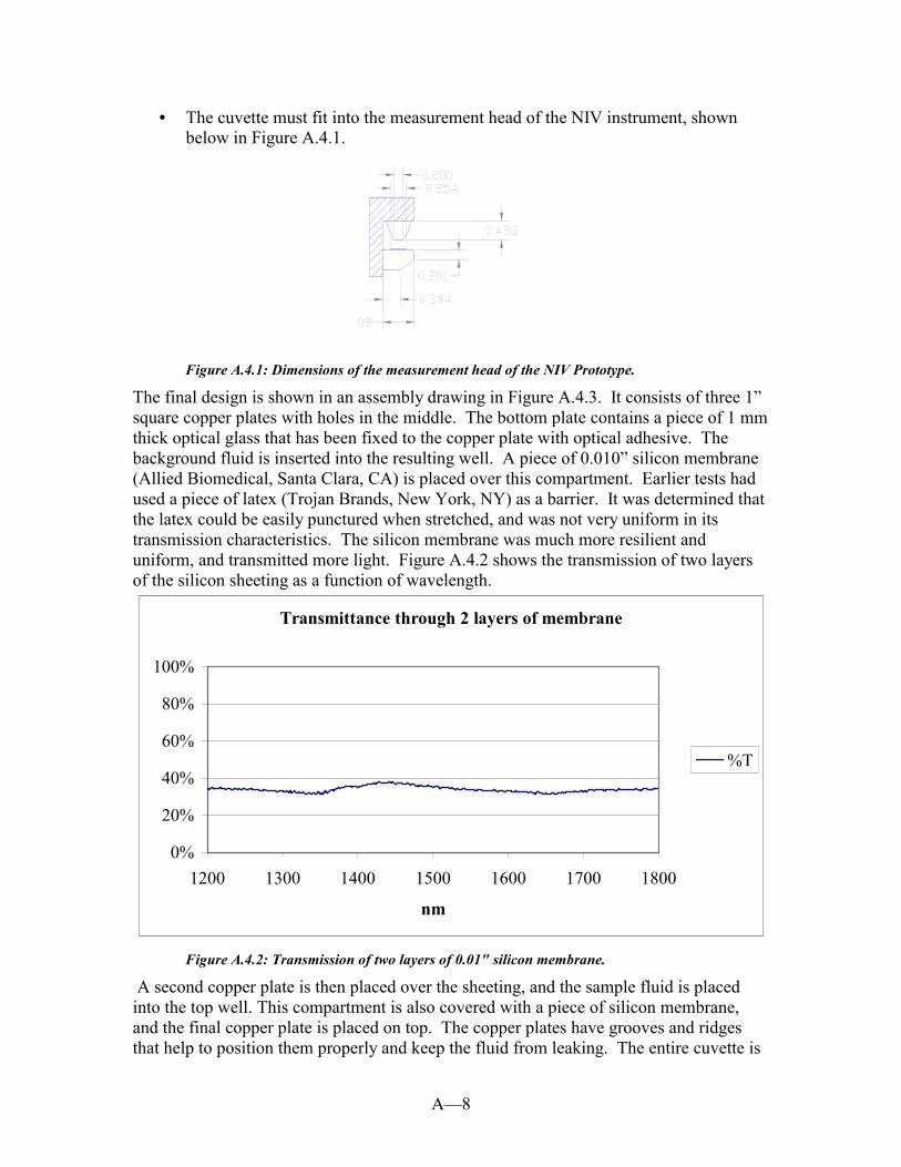
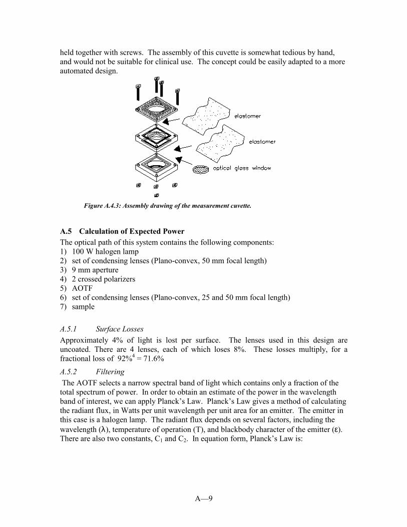
The final design is shown in an assembly drawing in Figure A.4.3. It consists of three 1” square copper plates with holes in the middle. The bottom plate contains a piece of 1 mm thick optical glass that has been fixed to the copper plate with optical adhesive. The background fluid is inserted into the resulting well. A piece of 0.010” silicon membrane (Allied Biomedical, Santa Clara, CA) is placed over this compartment. Earlier tests had used a piece of latex (Trojan Brands, New York, NY) as a barrier. It was determined that the latex could be easily punctured when stretched, and was not very uniform in its transmission characteristics. The silicon membrane was much more resilient and uniform, and transmitted more light. Figure A.4.2 shows the transmission of two layers of the silicon sheeting as a function of wavelength.

Transmittance through 2 layers of membrane

0%

20%

40%

60%

80%

100%

1200 1300 1400 1500 1600 1700 1800

nm

%T

Figure A.4.2: Transmission of two layers of 0.01" silicon membrane.

A second copper plate is then placed over the sheeting, and the sample fluid is placed into the top well. This compartment is also covered with a piece of silicon membrane, and the final copper plate is placed on top. The copper plates have grooves and ridges that help to position them properly and keep the fluid from leaking. The entire cuvette is

A—9

held together with screws. The assembly of this cuvette is somewhat tedious by hand, and would not be suitable for clinical use. The concept could be easily adapted to a more automated design.

Figure A.4.3: Assembly drawing of the measurement cuvette.

A.5 Calculation of Expected Power The optical path of this system contains the following components: 1) 100 W halogen lamp 2) set of condensing lenses (Plano-convex, 50 mm focal length) 3) 9 mm aperture 4) 2 crossed polarizers 5) AOTF 6) set of condensing lenses (Plano-convex, 25 and 50 mm focal length) 7) sample

A.5.1 Surface Losses Approximately 4% of light is lost per surface. The lenses used in this design are uncoated. There are 4 lenses, each of which loses 8%. These losses multiply, for a fractional loss of 92%4 = 71.6%

A.5.2 Filtering The AOTF selects a narrow spectral band of light which contains only a fraction of the total spectrum of power. In order to obtain an estimate of the power in the wavelength band of interest, we can apply Planck’s Law. Planck’s Law gives a method of calculating the radiant flux, in Watts per unit wavelength per unit area for an emitter. The emitter in this case is a halogen lamp. The radiant flux depends on several factors, including the wavelength (λ), temperature of operation (T), and blackbody character of the emitter (ε). There are also two constants, C1 and C2. In equation form, Planck’s Law is:

A—10

−

⋅=

⋅ 12

5

1

TC

e

CWλλ

ε, W/µm⋅cm2. (A.1)

(ε = 1, C1 = 3.74⋅104, C2 = 1.44⋅104, T = 3000 K) In order to find the power in a wavelength band, we must integrate this expression over the region of interest. In equation form, this integral is expressed as:

( )−⋅=

2

1

2 151

λ

λλ λ

λε de

CW TCb , W/cm2. (A.2)

It is possible to normalize this expression, to obtain the fraction of the total power that resides in a given band, rather than the W/cm2 form given above. The total power is given by:

4TWt ⋅⋅= σε , W/cm2. (A.3) The variable σ is Planck’s constant, which has a value of 5.67⋅10-12 W/cm2⋅K4. By dividing the expression for Wb by the expression for Wt, we obtain a fractional measure of the power in a given wavelength band. Note that this eliminates the need to for a value for ε or the area of the emitter. There is no closed form for the integral in equation A.2, but a numerical solution can be found. The software package Mathcad, Professional edition, v. 7.0 (Mathsoft, Inc.) was used for this purpose. The bandwidth of the AOTF which is being used for this project is approximately 7 nm. Figure A.5.1 shows the power spectrum of a lamp operated at a temperature of 3000 K. It also shows the integrated curve over the entire spectrum. To the right of the curve are three sample power bands. Each has a bandwidth of 7 nm to correspond to the AOTF bandwidth. The first calculation is the maximum power area of the band. This can be found by differentiating the Planck’s equation (A.1), setting it equal to zero, and solving for λ. The maximum power occurs at approximately 996 nm. The second band is the region we use for the Reference wavelength, and the third is the region we use for the Principal wavelength. Each of these bands contains approximately 0.47 % of the total lamp power, or approximately 0.47 W for a 100 W bulb. The transmission factor including surface losses and filtering effects is now 0.33%, or 0.33 W for a 100 W bulb.

A—11

Figure A.5.1: Power Spectrum for a halogen lamp being operated at 3000 K. The total power integration curve is shown by the solid line, while the dotted line shows the power per unit wavelength. Sample power calculations for several bands of interest are shown to the right of the figure.

A.5.3 Absorption/Polarization Losses Each polarizer transmits approximately 34% of the light that hits it. When crossed, the transmission drops to 0.2%. In parallel, they transmission averages 24%. Absorption also occurs in the sample. The sample contains two pieces of acrylic. In total, the transmission factor for the two acrylic pieces is 88.4%. There are also two Teflon ™ bags that each transmit 98% of light, for an overall transmission of 96%. The sample itself, if assumed to be mainly water, has an extinction coefficient of 39 m-1

at 1000 nm. This indicates that the sample will have approximately 26% transmission over a 1.5 cm maximum pathlength. Therefore, the overall transmission factor for the sample compartment is 22.1%. If the two crossed polarizers are included, the result drops to .044%. When the transmission for the filtering and surface effects in multiplied in, we now have a power of 146 µW, for a transmission factor of 1.46⋅10-4%.

A.5.4 Geometric The aperture limits the amount of light that can physically enter the optical path. The light intensity also falls off with the square of the distance from the source. This is necessary to meet the acceptance angle requirements of the AOTF, as well as to prevent excess broadband light from reaching the detector by physically blocking it from the path. The aperture opening is 9 mm in diameter. The aperture is located 66 mm from the center of the lamp filament. The aperture therefore subtends a solid angle of approximately 7.8° from the sphere of light that radiates from the filament. While this is slightly over the acceptance angle for the AOTF, it is a consequence of adjustments that were made to optimize the optical path after the components were made. It does not seem to significantly affect the operation of the device. In order to calculate the percentage of power in this 7.8° solid angle, it is necessary to find the percentage of the sphere surface that this covers. We can use the solid angle formula for this purpose. This formula states that the surface area on a sphere of the area subtended by a circular section is given by:

0

0.5

1

0.1 1 10

Wb( ),0.1 λ

W( )λ

λ

=Wb( ),.9925 .9995 0.004733

=Wb( ),.9265 .9335 0.004726

=Wb( ),1.0135 1.0205 0.004714

A—12

θθπ 2sin2)2cos1(2 =−=Ω , Ω in steradians. (A.4) To convert to sphere units, divide by 4π. Substituting 2θ = 7.8°, we find that the aperture lets through .463% of the light. The distance from source to detector also causes the power output to fall off by approximately a factor of 10. Our overall transmission figure, including surface, absorbtion, filtering, and geometric effects is therefore 6.8⋅10-8%, for an expected power output of 0.068 µW. Note that this is the maximum power expected, and will decrease as factors such as the light intensity decrease and factors such as the sample absorbance increase. This factor of 0.068 µW is merely an estimate which we can use to calculate the maximum allowable signal gain, as found in Appendix C.

B—1

APPENDIX B: SOFTWARE DESIGN The Urea Monitoring System (UMS) that has been developed as described in Chapters 5-7 requires an IBM compatible personal computer (PC) to control its operation, as it is not a standalone system. The requirements of the research prototype that has been developed here are different than would be required for a clinical instrument. This approach allows maximum flexibility in development of control algorithms for the UMS. For the purposes of this project a special software system was developed that supports urea concentration and clearance monitoring. The software system controls the operation of the urea clearance monitor, initiates urea level measurements, and collects, stores, and analyzes the recorded data. This software system runs under Microsoft Windows 3.1™ or higher and provides the operator with a graphical user interface (GUI). This provides a high level of automation and ease of use while still providing low-level access to the system parameters. The system data is shown graphically on the screen, and the operator is allowed to change the operating parameters in real time. The GUI also displays measured data values and results of the data analysis. The software system was developed using National Instruments’ Lab Windows/CVI™ (version 4.0) software development package. Lab Windows/CVI is a development tool that provides an interactive tool for developing C language programs. It is geared towards development of instrument control and data acquisition applications. In this chapter, the basic software structure of the UMS is described. The major system function, design, and operations are explained, as are basic user instructions where needed. All of the GUI controls are explained in terms of their purpose, action, and operating constraints. The goal of this chapter is to provide a reference for understanding and utilizing the UMS software system.

B.1 Software System Structure The UMS software system allows the operator to control the urea level measurements and the overall operation of the instrument. The program can change the UMS operating parameters, perform near-continuous urea level measurements, present both measured and calculated data, and store obtained results. A simplified block diagram of the software system is presented in Figure B.1.1.

B—2

Figure B.1.1: Urea Monitoring System Software block diagram.

The operator interacts with the software system through a GUI within the MS-Windows environment. The operator can select one of several options in the main interface window, and the software activates a corresponding function to handle the event. See § B.2 for more details about the GUI operation. The general functions that can be performed with this software system through the GUI are: • = Read current system parameters; • = Set new system parameters; • = Initiate a urea concentration measurement, save the output data and plot the results. • = Calibrate the urea measurement system and change, load, or save calibration data

files. The system may be in one of two modes of operation: Idle Loop or Measurement. In Idle Loop mode, the software system performs maintenance tasks only. It tries to maintain light intensities at certain target levels (This keeps the AOTF at a constant temperature, which in turn helps to keep the wavelength control more stable). It also updates an on-screen clock, updates measured data parameters, and checks for user input. If the user updates an on-screen parameter, the software sends a control command to adjust the hardware, and resumes the Idle Loop mode of operation. The other operation mode is the Measurement mode. In this mode, the system performs one urea concentration measurement when the user presses a button. A typical urea concentration measurement takes 80 seconds, after which the results are presented to the user. The results of the last 100 measurements are plotted on the GUI.

B.1.1 Idle Loop Operation During the normal (non-measurement) state of operation, the system is performing several simple tasks. It is continually reading the system parameters from the analog to digital converters, updating the display, and refreshing the digital to analog converters and wavelength controls. This update takes place approximately twice per second. (Display updates will be discussed further in § B.2)

GUI

Result Storage

Urea Measurements

Dialysis Efficiency

Measurements

model parameter

calculation/ application

Result Presentation

User

B—3

Figure B.1.2: Flowchart of the Idle Loop Control Software.

In addition to the normal updates, a second routine is entered once every 20 seconds. This routine tries to set a target light intensity by monitoring the received light at the input light detector. The target light intensity is read from the initialization file, and is usually on the order of 0.4 V. The system calculates the difference between DCIP and the target intensity, and ramps PRI_INT up or down by a value proportional to the difference. The converters are then read again, and this process is repeated iteratively until the actual intensity is within 1 mV of the target intensity. The process will also stop if PRI_INT gets above 10V or below 0V. This prevents the system from running away if the light bulb is turned off or is otherwise acting unusual. This target intensity setting protocol is invoked upon startup as well, immediately after the initialization file is read. For a description of the initialization file, see § B.1.5. A flow chart of the idle loop is given in Figure B.1.2.

B.1.2 Urea Measurements A urea measurement is initiated by the user through the GUI. (See § B.2). Once the start button is pressed, the system goes through several preparatory steps before any data is recorded. The system transfers approximately 8 ml of fluid from a water bath through the sample compartments in order to flush and prime the measurement cuvette. The clean dialysis fluid is then locked into the cuvette and the spent dialysate is evacuated, in order

Update System Parameters

Read System Data

20 loops done?

Does DC_IP match target?

Adjust PRI_INT

YES

YES

NO

NO

B—4

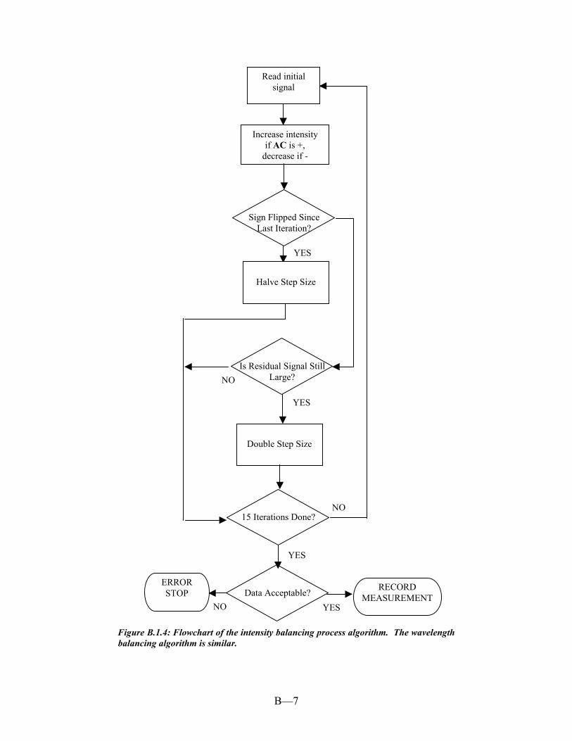
to allow balancing to begin. The system then moves the measurement head to the home position, and does a preliminary series of data integrity tests. The home position is the point at which the spent fluid compartment is completely compressed and the measurement head is slightly pressing on the clean fluid compartment (about 3mm into the compartment). This data integrity test checks the initial light intensity being received through the sample and the system temperature. The current values are tested against set limits. The value of these limits are set in the initial setup file (See § B.1.5). If any of the parameters are out of range, the measurement is stopped and the user is advised of the problem. If too much light has been received through the sample, then the sample compartment may have been inadequately filled. If too little light is being received from the sample, the problem may be more serious. In this case, the light bulb may be failing, or the AOTF may not be receiving adequate power. In either case, the user should attempt to correct the problem, and restart the measurement. The temperature conditions are also checked, and the user advised to make corrections if the values are out of scale. The overall measurement cycle is shown in flowchart form in Figure B.1.3. If the data conditions are acceptable, the balancing phase of the measurement begins at this point. The first task is intensity balancing. This involves adjusting the OFFSET signal iteratively until the AC signal is smaller than a given value. The size of this acceptance window is specified in the initial setup file. Increasing the OFFSET signal has the affect of increasing the REF_INT signal. This is accomplished by the PI Control loop in the hardware. The iterative balancing process proceeds as follows. The current value of the AC signal is read from the data converters. If this value is negative, the offset value is increased by an initial starting step. If the value is positive, the offset value is decreased by the same step size. This process is repeated 15 times. If the sign of the AC signal changes between successive iterations, the size of the step is cut in half. If the AC signal is still more than 0.5V from zero, the step size is doubled. Once fifteen iterations have been performed, the system checks to see if the AC signal is within the acceptance window. If not, the measurement is rejected and an error message is given. Otherwise, the measurement data is stored. The measurement head is then moved by the system to the wavelength balancing position, which involves a slight (approximately 2mm) decompression of the clean fluid compartment. The exact distance is specified by the balancing_distance parameter. The wavelength balancing procedure takes place in the same manner as the intensity balancing procedure. The only difference is that the Reference Wavelength is adjusted rather than the OFFSET signal. The flowchart of the balancing process is shown in Figure B.1.4. This figure shows the intensity balancing process, but would be the same for the wavelength balancing process. These two procedures are repeated twice, at which point, if successful, the system is considered balanced. During the second set of balancing iterations, a stray light recording is made by shutting off the intensity control signal to the AOTF after the balancing data has been recorded in that position. Stray light is defined as any residual detected light that does not originate from the first order beam of the AOTF.

B—5

The second phase of the measurement begins at this point. The measurement head is moved further out of the compartment, approximately 0.5mm, releasing the pressure on the spent fluid compartment. The exact distance is specified by the measurement_distance parameter. The system then transfers approximately 0.8 ml of spent dialysis fluid into the cuvette. The system data is then recorded. If there are more than three measurement positions specified, i.e. for a profile type measurement, the total measurement distance is divided by the number of measurement positions, and the measurement head moves in increments, while the system records data at all positions.

B—6

Figure B.1.3: Flowchart of a urea measurement cycle.

Move into home position

Test Data Integrity

Data Acceptable?

Intensity Balanced?

Balance Intensity

YES

NO ERROR STOP

ERROR STOP

Wavelength Balanced?

Balance Wavelength

ERROR STOP

2 Iterations Done?

Data Acceptable? ERROR STOP

RECORD MEASUREMENT

YES

YES

YESNO

NO

NO

YES

B—7

Figure B.1.4: Flowchart of the intensity balancing process algorithm. The wavelength balancing algorithm is similar.

Read initial signal

Increase intensity if AC is +,

decrease if -

Sign Flipped Since Last Iteration?

Is Residual Signal Still Large?

Halve Step Size

15 Iterations Done?

Data Acceptable? ERROR STOP

RECORD MEASUREMENT

YESNO

YES

Double Step Size

YES

YES

NO

NO

B—8

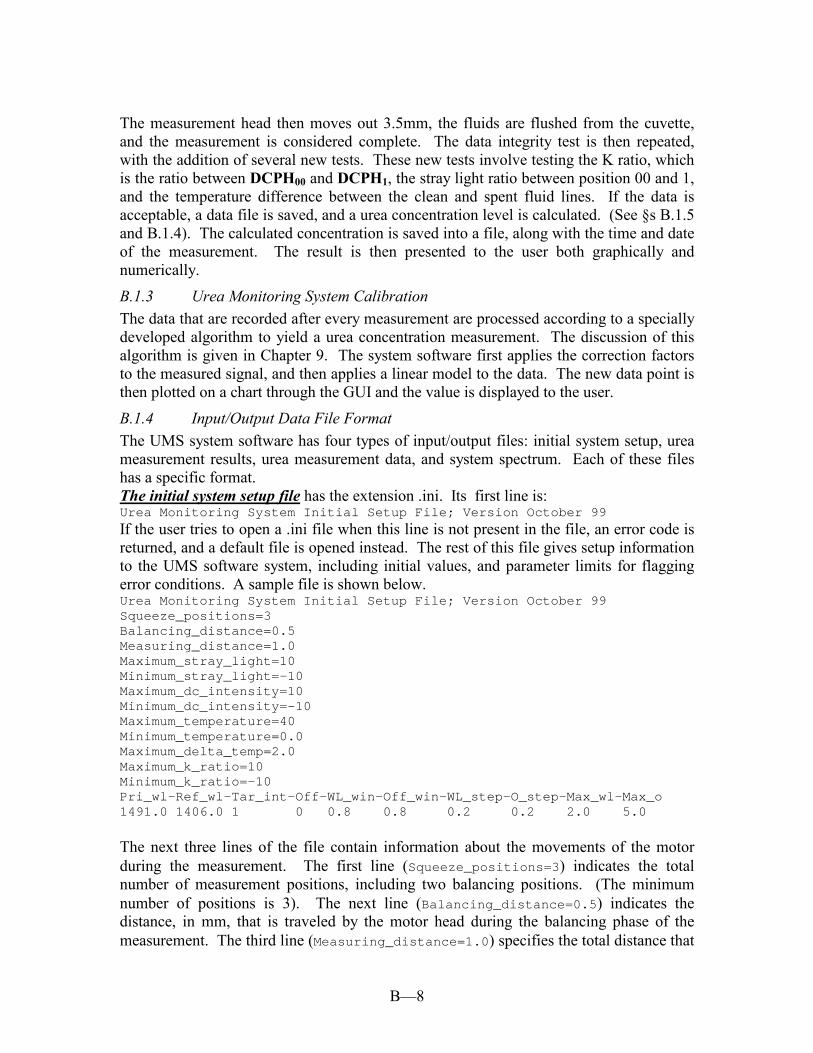
The measurement head then moves out 3.5mm, the fluids are flushed from the cuvette, and the measurement is considered complete. The data integrity test is then repeated, with the addition of several new tests. These new tests involve testing the K ratio, which is the ratio between DCPH00 and DCPH1, the stray light ratio between position 00 and 1, and the temperature difference between the clean and spent fluid lines. If the data is acceptable, a data file is saved, and a urea concentration level is calculated. (See §s B.1.5 and B.1.4). The calculated concentration is saved into a file, along with the time and date of the measurement. The result is then presented to the user both graphically and numerically.

B.1.3 Urea Monitoring System Calibration The data that are recorded after every measurement are processed according to a specially developed algorithm to yield a urea concentration measurement. The discussion of this algorithm is given in Chapter 9. The system software first applies the correction factors to the measured signal, and then applies a linear model to the data. The new data point is then plotted on a chart through the GUI and the value is displayed to the user.

B.1.4 Input/Output Data File Format The UMS system software has four types of input/output files: initial system setup, urea measurement results, urea measurement data, and system spectrum. Each of these files has a specific format. The initial system setup file has the extension .ini. Its first line is: Urea Monitoring System Initial Setup File; Version October 99

If the user tries to open a .ini file when this line is not present in the file, an error code is returned, and a default file is opened instead. The rest of this file gives setup information to the UMS software system, including initial values, and parameter limits for flagging error conditions. A sample file is shown below. Urea Monitoring System Initial Setup File; Version October 99Squeeze_positions=3Balancing_distance=0.5Measuring_distance=1.0Maximum_stray_light=10Minimum_stray_light=-10Maximum_dc_intensity=10Minimum_dc_intensity=-10Maximum_temperature=40Minimum_temperature=0.0Maximum_delta_temp=2.0Maximum_k_ratio=10Minimum_k_ratio=-10Pri_wl-Ref_wl-Tar_int-Off-WL_win-Off_win-WL_step-O_step-Max_wl-Max_o1491.0 1406.0 1 0 0.8 0.8 0.2 0.2 2.0 5.0

The next three lines of the file contain information about the movements of the motor during the measurement. The first line (Squeeze_positions=3) indicates the total number of measurement positions, including two balancing positions. (The minimum number of positions is 3). The next line (Balancing_distance=0.5) indicates the distance, in mm, that is traveled by the motor head during the balancing phase of the measurement. The third line (Measuring_distance=1.0) specifies the total distance that

B—9

the motor should travel during the measurement phase once balancing is complete. In other words, the motor should finish the measurement cycle at a distance equal to the sum of the balancing distance and the measurement distance, regardless of the total number of measurement positions. The next nine lines are used to specify error flagging limits on the data. The first two are minimum and maximum levels of stray light (Maximum_stray_light=10,Minimum_stray_light=-10). (Stray light is defined as any light that is detected that has not been derived from the first order beam coming from the AOTF. It is measured by shutting off the intensity control signal to the AOTF and measuring the level of the signal at the detector.) The second two lines specify limits for the initial amount of received light at the Sample Light Detector (SLD). (Maximum_dc_intensity=10,Minimum_dc_intensity=-10). A measurement outside of the limits may indicate a positioning error or failure of the lamp. The next three lines are concerned with the system temperature. (Maximum_temperature=40, Minimum_temperature=0.0,

Maximum_delta_temp=2.0). The first two specify a minimum and maximum temperature for the measurement, and the third specifies the maximum allowable temperature difference between the spent and clean fluid lines. The final two lines deal with the light absorbance ratio K. (Maximum_k_ratio=10, Minimum_k_ratio=-10). K is defined as the ratio between light transmittance at the thinnest sample distance and the thickest sample distance. (i.e. DCPH00/DCPH1) If this ratio is outside of acceptable limits, the sample may have been poorly compressed, or contained an air bubble, or else have been otherwise unacceptable. The next line in the file is a reference for the user who may need to modify the file. The line below it specifies ten parameters that are used to set initial parameters and to control the balancing process: Pri_wl-Ref_wl-Tar_int-Off-WL_win-Off_win-WL_step-O_step-Max_wl-Max_o

The first two parameters specify the Principal wavelength and the initial guess for the Reference wavelength, respectively. The third parameter specifies the target intensity that is recorded at the Input Light Detector (ILD). The fourth parameter is the offset, which controls the difference between DCIP and DCIR. The fifth and sixth parameters are error flagging limits as well. They specify the acceptable degree of residual AC signal after each stage of balancing. WL_win specifies the size of the acceptance window for wavelength balancing, while Off_win specifies the size of the acceptance window for intensity balancing. The seventh and eighth parameters (WL_step O_step) specify the initial step sizes that the system uses when beginning the balancing process. The final two parameters are currently unused. The urea measurement results file has the extension .umd. It contains one line for each measurement. Each line consists of a time, date, and urea level (in mg/dl). A sample line might read: 10:05:20 01/22/99 120

The most recent measurement appears at the end of the file. The urea measurement data file has the extension .ums. This file is used for parameter extraction and data analysis. It contains information about the system that was recorded

B—10

during the measurement. It also contains one line per measurement record. The individual data are comma-delimited in the file, and can be loaded into a spreadsheet such as MS-Excel for data analysis. The line begins with a measurement number, followed by the date and time, and then a marker for a calibrating urea level point. The principal and reference wavelength appear next, followed by the principal intensity, offset, and system bias. The next two pieces of data are the amount of time (in seconds) spent in each balancing position (wavelength and intensity). The rest of the line contains data about the system parameters as read during each phase of the measurement. For each parameter, at least three records appear, one for each measurement position (wavelength balancing, intensity balancing, and each measuring position). In other words, the next three pieces of information that appear in the file after the clock information are AC00, AC0, and AC1. Each signal that is entered into the data file follows this pattern. The order of the data is: AC, DCSP, DCSR, REF_INT, DCIP, DCIR, STRAY_I, STRAY_S, T_CLEAN, T_SPENT. A typical data file record line might appear as below: 10, 1/22/99, 10:05:20, &, 1491, 1406, 5.2, .1, .0073, 18.542, 12.412,0.0001213, 0.00012412, 0.0001921, .8987, .8354, .8001, .7632, .7654,.7521, 6.801, 6.802, 6.806, 1.1231, 1.1023 1.032, 1.2232, 1.2003,1.1032, .3564, .3654, .3546, .3465, .3401, .3321, 37.2, 37.2, 37.2,37.5, 37.5, 37.6

The system spectrum file has the extension .spc. The file has 400 lines, since the spectrum is recorded at 400 different wavelengths over the range from 800 to 1200 nm. The format of each line is the wavelength, followed by the SLD signal, and finally the ILD signal. A typical line might be: 1050 1.231 1.892.

B.1.5 Data Acquisition In § C.2, the DEM hardware system was described, including the implementation of the data acquisition system. Recall that all data acquisition for this system take place through the parallel port. The exception is the wavelength control, which is done through the ISA bus. In this §, the software required to control the data acquisition is presented. B.1.5.1 Parallel Port Operation The typical PC has between one and four parallel ports. We use the first parallel port, which is the device known as LPT1, or PRN to the PC. The parallel port has three 8 bit wide registers associated with it that can be programmed by the user. For the purposes of this research, we assume a standard mode of operation. This indicates that the registers are not bi-directional, except where stated. A complete description of the modes of operation (standard vs. enhanced) is beyond the scope of this dissertation, and will be omitted here). The first register usually resides at address 378h. This is the Data register. The signal configuration for this register is: Data Register (378h) Bit 7 6 5 4 3 2 1 0 Signal MOT_EN PUMP VALVE DIR SDATA SCLK LD_DA STRB

Any of these signals can be turned on or off with a simple write instruction to the Data register. For example, to turn on MOT_EN, the following instruction would be given: outp(0x378, 0xA0);

B—11

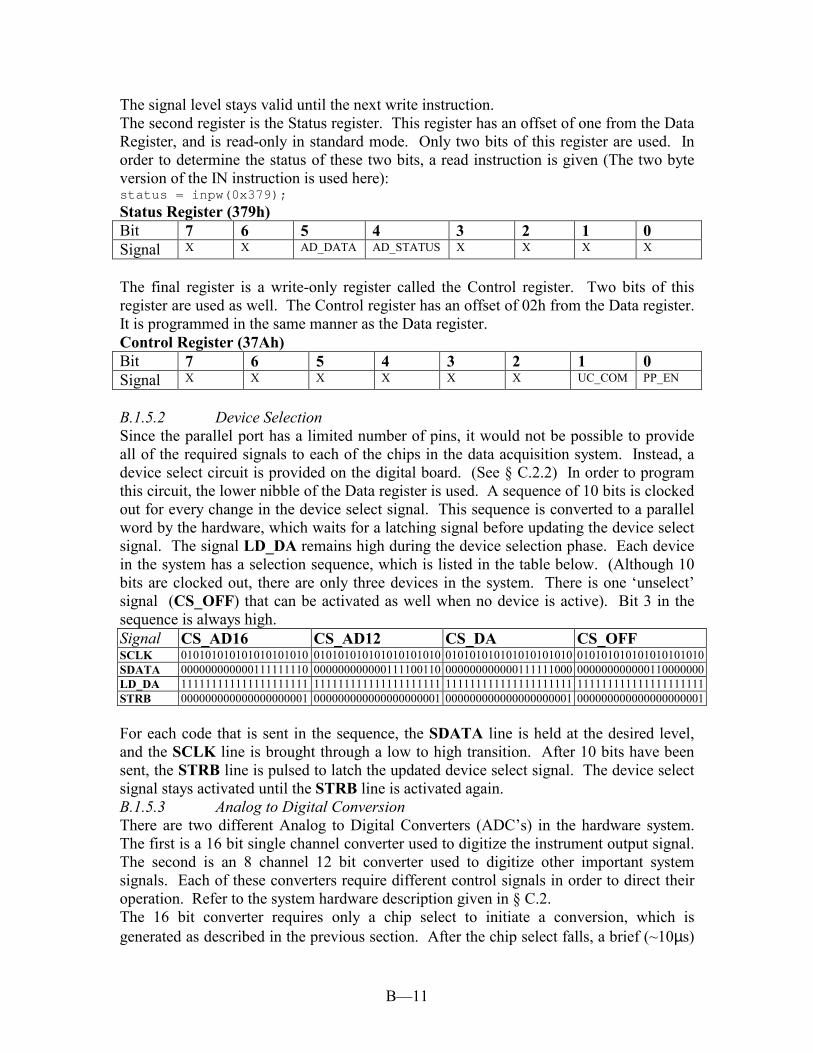
The signal level stays valid until the next write instruction. The second register is the Status register. This register has an offset of one from the Data Register, and is read-only in standard mode. Only two bits of this register are used. In order to determine the status of these two bits, a read instruction is given (The two byte version of the IN instruction is used here): status = inpw(0x379);

Status Register (379h) Bit 7 6 5 4 3 2 1 0 Signal X X AD_DATA AD_STATUS X X X X

The final register is a write-only register called the Control register. Two bits of this register are used as well. The Control register has an offset of 02h from the Data register. It is programmed in the same manner as the Data register. Control Register (37Ah) Bit 7 6 5 4 3 2 1 0 Signal X X X X X X UC_COM PP_EN

B.1.5.2 Device Selection Since the parallel port has a limited number of pins, it would not be possible to provide all of the required signals to each of the chips in the data acquisition system. Instead, a device select circuit is provided on the digital board. (See § C.2.2) In order to program this circuit, the lower nibble of the Data register is used. A sequence of 10 bits is clocked out for every change in the device select signal. This sequence is converted to a parallel word by the hardware, which waits for a latching signal before updating the device select signal. The signal LD_DA remains high during the device selection phase. Each device in the system has a selection sequence, which is listed in the table below. (Although 10 bits are clocked out, there are only three devices in the system. There is one ‘unselect’ signal (CS_OFF) that can be activated as well when no device is active). Bit 3 in the sequence is always high. Signal CS_AD16 CS_AD12 CS_DA CS_OFF SCLK 010101010101010101010 010101010101010101010 010101010101010101010 010101010101010101010SDATA 000000000000111111110 000000000000111100110 000000000000111111000 000000000000110000000LD_DA 111111111111111111111 111111111111111111111 111111111111111111111 111111111111111111111STRB 000000000000000000001 000000000000000000001 000000000000000000001 000000000000000000001 For each code that is sent in the sequence, the SDATA line is held at the desired level, and the SCLK line is brought through a low to high transition. After 10 bits have been sent, the STRB line is pulsed to latch the updated device select signal. The device select signal stays activated until the STRB line is activated again. B.1.5.3 Analog to Digital Conversion There are two different Analog to Digital Converters (ADC’s) in the hardware system. The first is a 16 bit single channel converter used to digitize the instrument output signal. The second is an 8 channel 12 bit converter used to digitize other important system signals. Each of these converters require different control signals in order to direct their operation. Refer to the system hardware description given in § C.2. The 16 bit converter requires only a chip select to initiate a conversion, which is generated as described in the previous section. After the chip select falls, a brief (~10µs)

B—12

delay is programmed to allow the conversion to complete. After the delay, 16 clock pulses are given using the SCLK signal. After the clock is brought low, a word is read from the Status register. The result is then masked to read the fifth bit. If the bit is a one, then the corresponding value of the bit is accumulated into the result. This result is in two’s complement format. In order to convert the bit result into a voltage, the accumulated value is divided by 3276.8. This translates to an LSB weight of 0.3055 mV. If the accumulated result is over 8000h, the result was negative, so the full scale range (20 Volts) of the converter is subtracted from the voltage value in this case. Once the conversion is complete, the chip select is released by activating the CSOFF signal. The second converter is somewhat more complex in its operation. Since it has eight channels, it requires a control word which is programmed serially into the device. This control word sets up the conversion parameters and selects the channel. The format of this control word is shown in Figure B.1.5. The device is operated in bipolar, single ended mode with an internal clock. The format of the control word is therefore 1xxx0110 where the xxx represents the channel selection bits. The channel selection bits and their corresponding signals are given below: Channel Code Signal 0 000 REF_INT 1 100 POSITION 2 001 TEMP1 3 101 TEMP2 4 010 DCIR 5 110 DCSR 6 011 DCIP 7 111 DCSP A conversion using this device also begins by activating the correct device select signal (CS_AD12). After this, the control word is clocked into the device using SCLK and SDATA. Once the last bit of the control word is clocked into the device, a conversion begins. As before, a brief delay (~10 µs) is programmed to allow the conversion to complete. The conversion result is read back in the same way as it was for the 16 bit converter. The data is read back from the device with a leading zero bit and three trailing zeroes that must be discarded from the conversion. This data is also in two’s complement format. The LSB weight of this converter is 1 mV, and the full scale range is 4.096V. For accumulated values over 8000h, 4.096 is subtracted from the voltage reading to yield a negative value. The chip select is then deactivated by programming the CS_OFF signal.

B—13

Figure B.1.5: Control word format for the 12 bit converter. (Taken from the MAX186 datasheet)

The software has an outer loop that completes several readings of each channel. The number of readings is selectable through the GUI. These readings are accumulated and averaged to improve the signal to noise ratio of the conversion. B.1.5.4 Digital to Analog Conversion The Digital to Analog Converter (DAC) is a four channel device, three of which are currently in use. This device is programmed by activating the corresponding device select line (CS_DA), and then sending a control word. This control word selects the desired channel, programs the mode of operation, and the desired voltage. The format of this word is [A1:A0 C1:C0 D11:D0]. C1 and C0 are always 0. For A1:A0, the format is: Channel A1:A0 Signal 0 00 OFFSET 1 01 - 2 10 PRI_INT 3 11 BRIDGE_OFFSET D11:D0 is calculated by converting the desired voltage to a bit stream in two’s complement format. The weight of the LSB is 4.88 mV. Once the final bit is programmed into the DAC using the SCLK and SDATA lines, the LD_DA signal is programmed to go low, causing the DAC to latch the signal onto the desired output channel. At this time, the chip select signal is released by activating CS_OFF. B.1.5.5 Motor Control Control of the motor is very straightforward. Three pins are programmed to control the number of steps and the direction. The hardware does the rest of the signal generation. The MOT_EN pin causes the signal SCLK to be connected to the motor control circuit. The state of the DIR pin can cause the driver chip to reverse the order of pulse sent to the

B—14

motor, causing the motor to spin in the opposite direction. If DIR is 0, the motor spins forward. The motor will spin backward when DIR is 1. In order to turn the motor one step, the MOT_EN pin is brought high, and SCLK is transitioned between low and high. A delay is programmed between the low to high transition to account for the motor’s response time. Each step corresponds to 1/200th of a full revolution. The physical system moves 1mm for each revolution, for a resolution of 5 µm. Once the motor has been turned the desired number of steps, the MOT_EN signal is brought low again, disabling the motor control circuit. During a motor movement, the desired position is checked against the value that is read from the Space Age Controls ™ position feedback device. The position is iteratively adjusted until the actual position is within .1mm of the desired value. B.1.5.6 Pump Control The software control of the pump is also very simple, as the actual state transitions of the pump driver circuit are done with an Altera™ chip. The pump only requires one software control signal, PUMP. In order to advance the pump motor one step, the PUMP signal must be pulsed low then high. The pump also requires at least a 10 ms delay between steps. One click is approximately 0.4 ml. This calibration is built into the software, so that a specific amount of fluid can be pumped as desired by the user. B.1.5.7 Solenoid Valve Control In order to keep the fluid in the Teflon bags during a measurement, a set of four solenoid pinch valves are used. In order to reduce the number of digital lines which are required to control these valves, an Altera™ chip was used to make a ‘state machine’. (See Appendix J for a hardware/firmware description of this system). In order to cause the valves to transition to their next state, two digital lines must be pulsed. The valve controller has eight states that correspond to different phases of the measurement. These states control whether fluid is being flushed or filling the measurement cuvette. There is an entrance and an exit valve for both compartments of the measurement cuvette. B.1.5.8 Wavelength Control In § C.2.4, the RF signal control hardware was discussed. Recall that there are two input controls to the device. The first is the intensity, which is an analog voltage. The second is the wavelength, which is a 32 bit digital control. This control word is converted in the NEOS driver to a frequency, which in turn selects the wavelength of light that is passed by the AOTF. The driver has a base frequency of 1024 MHz. In order to select the desired frequency, the following formula is used:

1024231⋅

= outfcode , where fout is expressed in MHz.

It is necessary to calibrate the driver frequency to the AOTF wavelength, since this control is not strictly linear. An external device called a monochromator is required to complete this calibration. This device, manufactured by CVI, Inc., has an entrance and exit slit that light can pass through. The device allows the user to select a desired wavelength of light to pass. In order to do the wavelength calibration, the monochromator is placed so that the slit is in line with the light path of the UMS. An external silicon detector is placed at the exit slit of the monochromator. This detector will only see a signal when both the monochromator and the AOTF are passing the same wavelength. The wavelength range of the AOTF is 1100 to 1800 nm, so the

B—15

monochromator is set to 1100 nm at the start. The frequency sent to the driver is stepped in increments of 1 MHz, until an increase in signal is seen at the detector. The frequency increment is decreased at this time, and the frequency at which the maximal signal occurs is recorded . The monochromator wavelength is then increased, and the calibration continues in the same manner. Approximately 30 points are recorded. This data is then entered into a Microsoft ® Excel spreadsheet. A five point multiple linear regression is performed on the data in order to obtain a calibration curve. The coefficients from the MLR are then used in the software to convert the desired wavelength to the necessary drive word. The fifth order polynomial coefficients obtained from the MLR are: order coefficient a 4.505027194752E+03 b -1.821738083231E+01 c 3.049222842297E-02 d -2.560096270007E-05 e 1.070483944157E-08 f -1.778722430193E-12 The frequency is then calculated as f = a + b·wl + c·wl2 + d·wl3 + e·wl4 + f·wl5. In order to set the wavelength, the calculated drive word is sent to the RF control card that resides on the PC’s ISA bus at a base address of 400h. This control card has four byte wide registers. The first two hold the control word for the principal wavelength, and the second two hold the control word for the reference wavelength. The controller card sends these two words to the NEOS driver in an alternating fashion at the frequency specified by CLK_REF, which is connected to the card through a 2 mm microphone jack. Since the PC has no 32 bit data writing (output) instruction, the control word must be broken into a high byte and a low byte. The low byte is determined by ANDing the number with the hexadecimal value FFFFh. The high byte is determined by left shifting the number 16 places, then ANDing the result with the hexadecimal value FFFFh. The result is then sent out with a byte wide output instruction

B.2 Urea Monitoring System Graphical User Interface In order to simplify the operation of the UMS, a graphical user interface (GUI) was developed. The main functions of the GUI is to provide a means by which the user can control the hardware, initiate measurements, and monitor the status of the system. This interaction is accomplished by means of window controls and/or window menus. The main GUI window contains several groups of function controls in the form of text boxes, control buttons, and indicators. These controls may give information to the user about the system, or be used to activate subroutines and hardware changes. Most of the function buttons in the window correspond to an element in the pull-down menu as well. When one of the function buttons or menu items is activated by the user, the GUI sends a control event code to the software, and the desired subroutine is carried out. When no user or system events are pending, (user events occur when a button is clicked, a value is changed, or a menu item is activated; system events occur when hardware

B—16

interrupts or timer interrupts are present), the GUI is operating in idle mode. This frees the system to perform necessary tasks. The GUI stays in idle mode until a system or user event intervenes. Once the event is handled, the GUI returns to idle mode and waits for the next event. The GUI for this system consists of four windows for controlling and optimizing the system and presenting results: • = Main Urea Monitoring System Window – allows the user to setup the hardware,

initiate measurements, load and save initial system configuration files, and change other operating and calibration parameters.

• = System Spectrum Window – displays the transmittance of the system as a function of frequency over the useful range of the AOTF. This is mainly a diagnostic tool, since the spectrum will show large deviations when the light bulb is beginning to fail. It may also help diagnose problems with the detectors or the AOTF.

• = Noise Analysis/Bias Cancellation Window – displays the level of system noise and the hardware system bias.

• = Stray Light Optimization Window – displays the stray light ratio for the system. The stray light ratio is defined as the amount of received light at the input light detector when the light intensity is at full scale versus when the light intensity is at zero.

B.2.1 Main User Interface The main user interface window is shown in Figure B.2.1. This window is titled “Optical Bridge Urea Monitoring System”. Twenty-two groups of controls are found on the figure: 1. Start Measurement – The user initiates a measurement by pressing this button. An

indicator light informs the user whether or not the instrument is ready to begin a measurement.

2. Quit – Pressing this button will terminate the session. 3. System Time – Output control for displaying the present time. 4. Motor Indicators – This is a set of two LED output controls that indicate when the

motor is in motion and in which direction it is turning. When the motor turns forward, the direction indicator turns yellow. When the direction is reversed, the direction indicator is blue.

5. Measurement Progress Indicators – This is a set of three LED’s and a slide control that indicate the progress of a measurement. The first LED is labeled Ready to Start. This indicates that the system is currently able to begin a measurement. The second LED is labeled Balancing. This LED is used to indicate the a measurement is in progress, and that the system is attempting to balance the background signal. The final LED is labeled Measuring. This LED indicates that the system has successfully been balanced, and the measurement phase has begun. The slide control is used to indicate the current position of the measurement head: intensity balancing, wavelength balancing, or measuring.

6. Pump Volume – Output control for displaying the amount of fluid that is being pumped through the system.

7. Elapsed Time – Output control for displaying the total length of the measurement, in seconds.

B—17

8. Urea Measurement Graph – Output control graph used to display a record of recent urea readings. The points show the 100 most recent readings.

9. AC and Normalized AC – This is a set of output controls that show the value of the raw signal and the normalized signal (raw signal divided by DCSP) as well.

10. DC Values – These four output controls show the four DC components of the signal: DCSP, DCSR, DCIP, and DCIR.

11. Loop – This output control shows the value of the Reference Wavelength Intensity (REF_INT), otherwise known as the loop voltage.

12. System Bias – This is the voltage, in mV that is set on the third DA channel to cancel the offset in the signal. The system bias is determined from the noise analysis.

13. Head Position – This control is a slide control that indicates the position of the measurement head. The zero position is when the head is fully closed. The rightmost control in this group shows the actual position (as read by the AD converter from the Space Age Controls potentiometer). The left control is the position which was set by the user or the software.

14. System Temperature – This is a set of two thermometer controls that display the current temperature of the spent and clean dialysis fluid lines.

15. File Utilities – This set of buttons will open a File Utilities dialog box, either to save or open an initial setup file.

16. User Profile – This text box gives the name of the current setup file. 17. Number of Averages – This is an input control that is used to control the number of

averages that is done every time the A/D converters are read. Repeating and averaging the readings improves the signal to noise ratio of the measurement by a factor of 2 .

18. Hardware Setup – This set of four input/output controls are used to control the intensity and wavelength of the light beam. The first two controls are used to control the wavelength of the principal and reference wavelength. The third control is the offset, and the final control is the principal intensity.

19. Model – This final control box allows the user to input a slope and an intercept for the linear model relating the signal to the urea concentration.

20. Valve – This control directs the hardware to advance the state of the solenoid pinch valves.

21. Pump – This control allows the user to pump a specified amount of fluid through the system.

22. AC Strip Chart – This control, only used for testing purposes, is a strip chart that plots the value of the normalized signal over time.

B—18

Figure B.2.1: The main user interface window for the UMS software system.

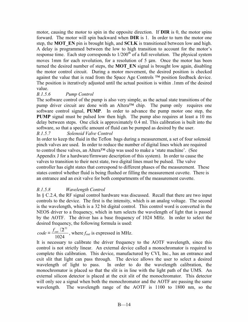
B.2.2 System Spectrum Window The user may access a system spectrum function through the Spectrum Analysis menu option. Once this function is called, a second window opens up that contains a large graph. See Figure B.2.2. Three buttons appear at the bottom of the window. The first is labeled Acquire, the second is labeled Save Data, and the final is labeled Quit. Pressing the Acquire button will start a spectral acquisition, which measures all four DC signals over the wavelength range of 1100 to 1800 nm. The wavelength is stepped in units of 2 nm. After the scan is complete, the spectral data is plotted in the graph window. Pressing the Save Data button will open a file dialog box, and the user can save a file with the extension .spc that contains the spectral data.

B—19

Figure B.2.2: The system spectrum window from the UMS system software

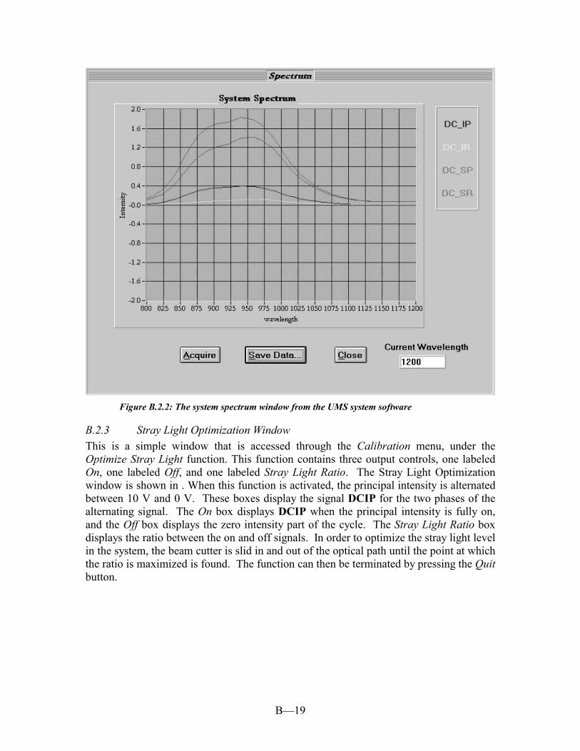
B.2.3 Stray Light Optimization Window This is a simple window that is accessed through the Calibration menu, under the Optimize Stray Light function. This function contains three output controls, one labeled On, one labeled Off, and one labeled Stray Light Ratio. The Stray Light Optimization window is shown in . When this function is activated, the principal intensity is alternated between 10 V and 0 V. These boxes display the signal DCIP for the two phases of the alternating signal. The On box displays DCIP when the principal intensity is fully on, and the Off box displays the zero intensity part of the cycle. The Stray Light Ratio box displays the ratio between the on and off signals. In order to optimize the stray light level in the system, the beam cutter is slid in and out of the optical path until the point at which the ratio is maximized is found. The function can then be terminated by pressing the Quit button.

B—20

Figure B.2.3: The Stray Light Optimization Window from the UMS system software

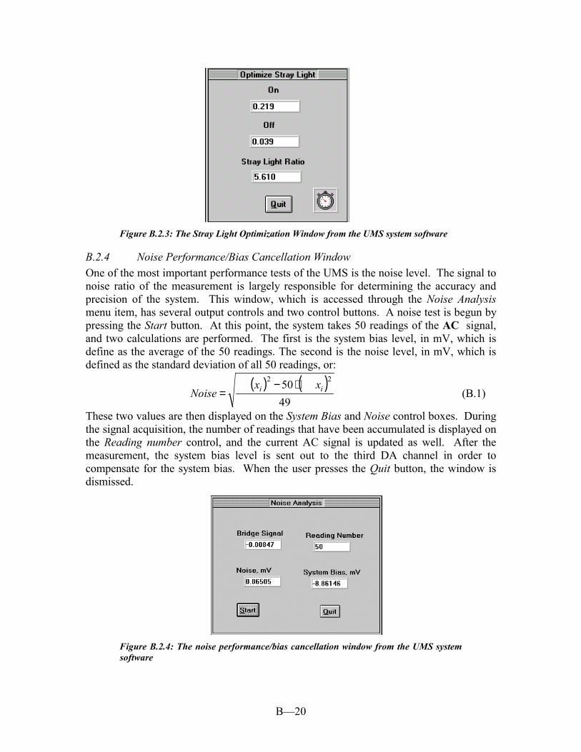
B.2.4 Noise Performance/Bias Cancellation Window One of the most important performance tests of the UMS is the noise level. The signal to noise ratio of the measurement is largely responsible for determining the accuracy and precision of the system. This window, which is accessed through the Noise Analysis menu item, has several output controls and two control buttons. A noise test is begun by pressing the Start button. At this point, the system takes 50 readings of the AC signal, and two calculations are performed. The first is the system bias level, in mV, which is define as the average of the 50 readings. The second is the noise level, in mV, which is defined as the standard deviation of all 50 readings, or:

( ) ( )4950 22 ⋅−

= ii xxNoise (B.1)

These two values are then displayed on the System Bias and Noise control boxes. During the signal acquisition, the number of readings that have been accumulated is displayed on the Reading number control, and the current AC signal is updated as well. After the measurement, the system bias level is sent out to the third DA channel in order to compensate for the system bias. When the user presses the Quit button, the window is dismissed.

Figure B.2.4: The noise performance/bias cancellation window from the UMS system software

B—21

B.2.5 The GUI Menu Bar The UMS menu bar contains five pull down menus: File, Start Acquisition, Calibration, Scans, and Noise. File: This menu, shown in Figure B.2.5, provides functions for handling the initial setup files and for quitting the UMS system software. 1. Read Setup – Opens an existing initial setup file 2. Save Setup – Saves the current initial setup file, either with the same name or a new

name. 3. Quit – ends the current session of the UMS system software. File… Start Acquisition… Calibration… Scans… Noise … Read Setup… Save Setup… Quit

Figure B.2.5: The menu bar and File pull down menu from the UMS system software.

Start Acquisition: This menu, shown in Figure B.2.6, will begin either a series of continuous urea measurements or a single urea measurement. 1. Perform Urea Measurement – This menu option will begin a single urea

measurement as described in § B.1.2. File… Start Acquisition… Calibration… Scans… Noise… Perform Urea Measurement

Figure B.2.6: The menu bar and Start Acquisition pull down menu from the UMS system software.

Calibration: This menu, shown in Figure B.2.7 offers functions for optimizing and calibrating the UMS system software. 1. Enter Calibration Point – This function can be used before or after a urea

measurement to enter a urea reading that has been obtained by an external method. 2. Optimize Stray Light – This menu option opens the stray light optimization window.

The operation of this window is described in § B.2.3 File.. Start Acquisition… Calibration… Spectrum Analysis… Noise Analysis… Enter Calibration Point Optimize Stray Light

Figure B.2.7: The menu bar and Calibration pull down menu from the UMS system software.

Scans: This menu, shown in Figure B.2.8, opens the spectrum analysis window. The operation of this window is described in § B.2.2. File… Start Acquisition… Calibration… Scans… Noise … Spectrum

Figure B.2.8: The menu bar and Spectrum Analysis pull down menu from the UMS system software.

B—22

Noise Analysis: This menu, shown in Figure B.2.9, opens the noise analysis/bias cancellation window. The operation of this window is described in § B.2.4. File… Start Acquisition… Calibration… Spectrum Analysis… Noise Analysis… Start

Figure B.2.9: The menu bar and Noise Analysis pull down menu from the UMS system software.

C—1

APPENDIX C: DIALYSIS EFFICIENCY MONITOR HARDWARE DESIGN

There are two major hardware sections in this system. The first is the instrumentation section, and the second is the IBM compatible personal computer (PC). The instrumentation section is responsible for controlling the wavelength and intensity of the delivered light, as well as detecting, amplifying, filtering, and processing the light that passes through the sample. The PC is responsible for controlling the instrumentation system, and for collection, storage, and processing of the recorded data. In this chapter, we describe the hardware of the dialysis efficiency monitor (DEM), including the realization of the Optical Bridge system. The hardware modules of the system are discussed and presented in detail with regards to their performance specifications, intended function, and design. Complete schematics of all modules are given in Appendix A.

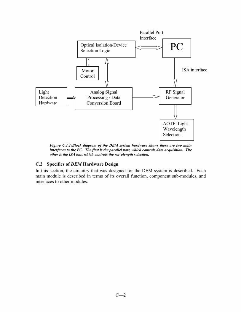
C.1 Hardware Modules There are several functions that the hardware performs in order to accomplish the measurement. shows a block diagram of the overall system. The PC directs the operation of all hardware modules. The PC used for this project has a Pentium processor (90 MHz) with a MS-Windows 95™ operating system. (This is the minimum set of system requirements.) There are five main modules that comprise the instrumentation system. These modules are listed in Figure C.1.1, together with names of the sub-modules, their basic tasks, and how the modules interface to the PC and/or the other modules. In the following section, we will begin to discuss each of the modules and their component parts.

C—2

Figure C.1.1:Block diagram of the DEM system hardware shows there are two main interfaces to the PC. The first is the parallel port, which controls data acquisition. The other is the ISA bus, which controls the wavelength selection.

C.2 Specifics of DEM Hardware Design In this section, the circuitry that was designed for the DEM system is described. Each main module is described in terms of its overall function, component sub-modules, and interfaces to other modules.

PC

Parallel Port Interface

Motor Control

Optical Isolation/Device Selection Logic

Analog Signal Processing / Data Conversion Board

ISA interface

RF Signal Generator

Light Detection Hardware

AOTF: Light Wavelength Selection

C—3

Table C.2.1:Hardware Modules that comprise the Dialysis Efficiency Monitoring system (I: Input, O: Output, B: Bidirectional)

Module Name Interfaces (Input/Output/Bidirectional)

Sub-modules Contained

Digital Board 1. PC (B) 2. Motor (B) 3. RF (O) 4. Analog Board (B) 5. Pump Control (O)

1. Optical Isolation Unit 2. Device Select Circuitry 3. Clock Generator Circuitry

Analog Board 1. Digital Board (B) 2. Detector Boards (2) (I)

1. Signal Transducers/Pre-Amplifiers and Filters (2)

2. Signal Demodulator 3. Lock in Amplifier 4. PIC Intensity Controller 5. Analog to Digital Converters 6. Digital to Analog Converters 7. Temperature Monitor

Motor Controller 1. Digital Board (B) 1. Stepper Motor Controller Pump and Temperature Controller

1. Digital Board (B) 1. Temperature Controller 2. Pump Controller

RF Signal Generator

1. AOTF (O) 2. Digital Board (O) 3. PC ISA slot (I)

1. Frequency controller card 2. Direct Digital Synthesizer Unit 3. Power Amplifier

C.2.1 Analog Board The Analog Board is responsible for most of the hardware signal processing. It is a four layer Printed Circuit Board (PCB). It has two trace layers, an analog ground plane, and a digital ground plane. The dimensions of the board are approximately 6” by 8”. Professor Stevan Kun of the Biomedical Engineering Department at WPI was responsible for much of the design of both the analog and digital boards. C.2.1.1 Signal Transducers/Amplifiers In addition to the main analog board, there are also two small signal boards that are considered part of this module. These signal boards contain the light detectors, current to voltage converters, and pre-amplifiers that are used to convert the received light to an electrical signal. The first signal board, called the Input Light Detector (ILD), is used to provide a reference, or normalizing factor for the signal. Its optical detector is strategically placed in the light path so that it receives a small portion of the light that enters the sample compartment. The ILD board transduces the light signal to a current, converts the current to a voltage, amplifies and filters this signal. The signal from the ILD used to normalize the signal from the other detector board, the Sample Light Detector (SLD). The SLD is used to record the light intensity at the exit of the sample compartment. See Chapter Appendix A: for a description of the placement of the two detector boards. The optical signal is in the range of a few microWatts (µW). The

C—4

photodetector that is used for this system is an Indium Gallium Arsenide (InGaAs) type. Its sensitivity bandwidth is 800 to 1700 nm. The absolute responsivity of the detector is defined as the current produced per Watt of optical power that reaches the detector. For this detector, the maximum responsivity is approximately 1 A/W. Figure C.2.1 shows a plot of the responsivity of an InGaAs detector. The maximum signal power reaching the detector is expected to be on the order of 0.07 µW, which will yield a maximum of 0.07 µA of signal from this detector‡. We desire a maximum signal output of 10 V. This means that our signal amplifier should have a gain of 1.5⋅108 Volts/Amp. The gain in this part of the circuit is approximately -1⋅106 V/A. (The rest of the gain is produced in a later stage). Since the photodetector produces a current, the necessary amplifier must convert the current to a voltage. It must also filter the signal in order to improve the signal to noise ratio. The light signal is switched between the Principal and Reference wavelength at a frequency of 60 Hz. The cutoff frequency for the low pass filter in the amplifier circuit is about 600 Hz, which was chosen to pass several harmonics of the received light intensity signal, which has a fundamental frequency of 60 Hz.

‡ The figure of 0.07 µW is arrived at by calculating the percentage of power from the 100 W lamp which arrives at the detector. This calculation involves geometrical considerations, surface losses, and sample absorbances. This calculation is performed in Chapter Appendix A:.

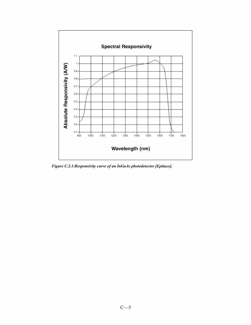
C—5

Figure C.2.1:Responsivity curve of an InGaAs photodetector [Epitaxx].

D—1

APPENDIX D: INTERFERING SUBSTANCE ABSORBANCE TABLE

Substance/structure[78]

mol. wt. [78]

significant bands (nm) [78]

[Level], mg/dl [90]

Notes [91]

Urea O || H2NCNH2

60.06 5945, 3092, 2906 70 major marker

glucose CH2OH H OH H OH OH H OH H H OH

180.16 3017, 7460 100 Present in dialysate

1-Methylguanidine NH || H2N-C-N-CH3 H

73.10 6024, 3680, 3158, 2910

0.00424 product of putrefaction

guanidine NH | H2NCNH2

59.07 6095, 3665, 3289 0.00141 strong organic base

Creatinine O || NH =NH N CH3

113.12 6283, 5991, 3074 0.7 End product of Creatine catabolism

Creatine NH O || || H2N-C-N-CH2-C-OH CH3

131.13 5905, 3230, 2997 0.45 Present in muscle tissue, normally excreted as creatinine

Arginine NH2 | H2NCNH(CH2)3CHCOH || || NH O

210.24 5861, 3064, 2863 1.87 Essential amino acid

Homoarginine NH2 | H2NCNH(CH2)4CHCOH || || NH O

224.26 6007, 3637, 3150 0.983 Amino acid

Phenol OH

94.11 6672, 6268, 2965 0.0083 Derived from coal tar. Higher levels in smokers and miners

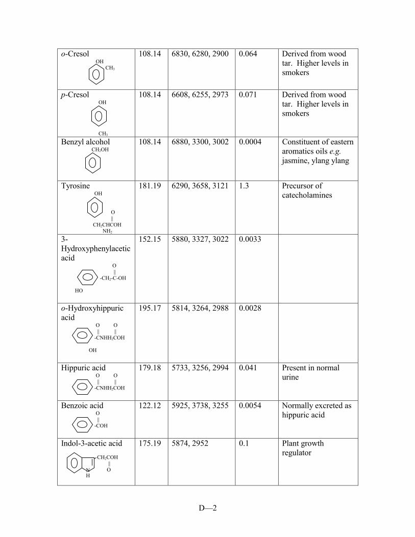
D—2

o-Cresol OH CH3

108.14 6830, 6280, 2900 0.064 Derived from wood tar. Higher levels in smokers

p-Cresol OH CH3

108.14 6608, 6255, 2973 0.071 Derived from wood tar. Higher levels in smokers

Benzyl alcohol CH2OH

108.14 6880, 3300, 3002 0.0004 Constituent of eastern aromatics oils e.g. jasmine, ylang ylang

Tyrosine OH O || CH2CHCOH NH2

181.19 6290, 3658, 3121 1.3 Precursor of catecholamines

3-Hydroxyphenylacetic acid O || -CH2-C-OH HO

152.15 5880, 3327, 3022 0.0033

o-Hydroxyhippuric acid O O || || -CNHH2COH OH

195.17 5814, 3264, 2988 0.0028

Hippuric acid O O || || -CNHH2COH

179.18 5733, 3256, 2994 0.041 Present in normal urine

Benzoic acid O || -COH

122.12 5925, 3738, 3255 0.0054 Normally excreted as hippuric acid

Indol-3-acetic acid CH2COH || O

175.19 5874, 2952 0.1 Plant growth regulator

NH

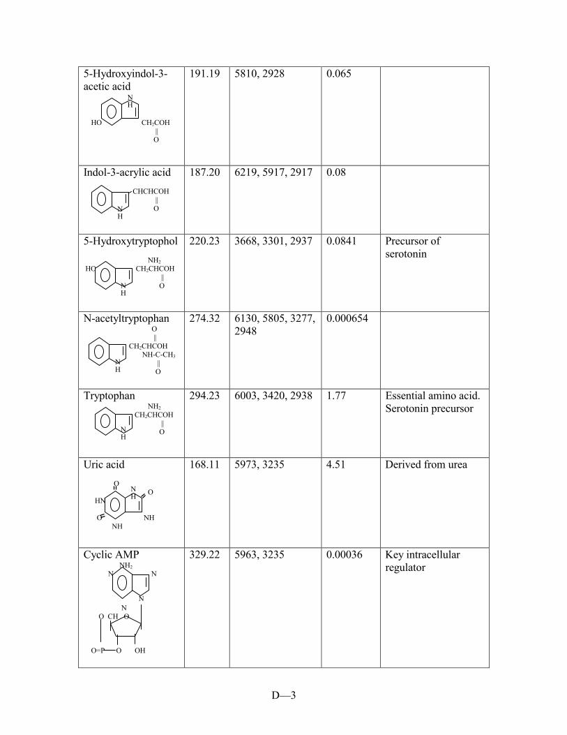
D—3

5-Hydroxyindol-3- acetic acid HO CH2COH || O

191.19 5810, 2928 0.065

Indol-3-acrylic acid CHCHCOH || O

187.20 6219, 5917, 2917 0.08

5-Hydroxytryptophol NH2 HO CH2CHCOH || O

220.23 3668, 3301, 2937 0.0841 Precursor of serotonin

N-acetyltryptophan O || CH2CHCOH NH-C-CH3

|| O

274.32 6130, 5805, 3277, 2948

0.000654

Tryptophan NH2 CH2CHCOH || O

294.23 6003, 3420, 2938 1.77 Essential amino acid. Serotonin precursor

Uric acid O O HN O NH NH

168.11 5973, 3235 4.51 Derived from urea

Cyclic AMP NH2 N N N O CH O O=P O OH

329.22 5963, 3235 0.00036 Key intracellular regulator

NH

NH

NH

NH

NH

NH

N

D—4

Amino acids (e.g. glycine) O || H2N-CH2-C-OH

75.07 6270, 3829, 3299 15 Non-essential amino acid. Inhibitory neurotransmitter

Mannitol CH2OH | HOCH | HOCH | HCOH | HCOH | CH2OH

182.17 7045, 3042 1.44 Anticaking agent. Poorly excreted by diseased kidneys, often used as a diagnostic aid

Oxalate O O O || || || HO-C=CH2-C-C-OH

132.07 6088, 5819, 3784, 3308

0.12 Part of urea cycle

Glucuronamide O || C-NH2 | O OH | | HO | | OH

193.16 6066, 2944 0.0054 Formed in liver to detoxify poisonous hydroxyls, especially chloral hydrate, morphine, camphor, or turpentine

Glycols O || HO-CH2-C-OH

76.05 5780, 3904, 3328 0.0065 Derived from reduction of oxalates during the urea cycle

Xanthine O HN O NH NH

152.11 6371, 5877, 3192 0.006 derived from guanine

Hypoxanthine O HN N N

136.11 6328, 5990, 3285 0.0063 Formed from the breakdown of nucleic acids

Putrescine NH2(CH2)4NH2

88.15 6250 0.02 Precursor to spermidine

Spermine H2N(CH2)3NH(CH2)3CH2NH | (CH3)3N H2

202.35 6234, 3418, 3041 0.008 Formed from spermidine

N

NH

D—5

Spermidine NH2(CH2)4NH(CH2)3NH2

145.2 6224, 3968, 3652 0.02 Formed from Putrescine. First found in sperm

Dimethylamine H2CNCH3 H

45.09 6085, 3386, 2924 0.14 Formed from methanol and ammonia

Water 18.02 6117, 3087, 2902 98%

E—1

APPENDIX E: HUMAN SUBJECTS STUDY PROTOCOL Project # 683

Saint Vincent Hospital/Fallon Clinic/Fallon Community Health PlanChart Review Study

This particular form may be used for chart review studies only.Please answer all questions. We can only accept completed forms.Please attach the formal protocol (if available) and a copy ofyour chart abstraction form. The attached finance form will needto be completed only for funded projects.

1. PROJECT TITLE:

Evaluation of Performance in Human Dialysate Solutions of a New Urea Monitor

2. PRINCIPAL INVESTIGATOR & INSTITUTION:

Robert A. Peura, PhD. Worcester Polytechnic Institute Rebecca A. Kupcinskas, ME Worcester Polytechnic Institute

3. FALLON OR SVH LIASON(S) AND DEPARTMENT (IF DIFFERENT):

Dr. Robert M. Black, Renal Medicine

4. PURPOSE OF STUDY:

A new urea monitor has been developed for the purpose of monitoring urea levels in spent hemodialysis fluid. This study is intended to provide clinical validation in terms of accuracy for the urea monitor. We intend to publish the results of this study in a peer-reviewed journal.

5. PLAN OF INVESTIGATION: (Include: length of study; how subjectswill be selected; approximate number of records that will bereviewed.) PLEASE INCLUDE A COPY OF THE DATA ABSTRACTION FORM.

Spent (used) hemodialysate solution will be obtained from 15 patients in the St. Vincent Hospital Dialysis Unit. The patients will be chosen randomly from the patient population on a single day. Hepatitis B antigen patients will be excluded. For each patient, a 20 ml sample will be obtained from the spent (waste) dialysate line at three times during the dialysis session, for a total of 45 samples. Off site we will then analyze these samples for their urea concentration and determine the urea concentration by standard independent means.

6. METHOD FOR COLLECTING DATA: How will the data be collected andwho will be extracting the information? (Will the information beextracted from the medical record and/or through a computerterminal?)

A clean 20 ml syringe will be used to sample the waste stream. A clean 20 ml sample vial will be filled and identified by number with no patient identification. The samples will be frozen for later analysis offsite. All personnel who handle the samples will be

E—2

required to wear protective gloves, and all work areas will be wiped with bleach after testing.

E—3

7. SUBJECT CONFIDENTIALITY:

A. Will the data be recorded whereby human subjects can be identified (either directly or indirectly through identifiers linked to subjects)?

No identification of the patient will be associated with the spent hemodialysis sample.

B. Where will patient’s names be kept and who has access to these names? N/A C. Where will data be kept and who has access?

PLEASE NOTE THAT ALL RESEARCH RECORDS MUST BE KEPT IN A LOCKED DRAWER.

8. FUNDING: How will this research be supported?

A) Source of funding________________________Both internal and external funding sources should be listed. Please complete attached finance form. _____X_________ There is no funding.

B) What Clinic/Hospital Resources will be required to conduct the study? (i.e. personnel, equipment, supplies)

None.

SIGNATURES:

_________________________ _________________________ __________________ Principal Fallon or SVH SignatureInvestigator Investigator Division Director --------------------------------------------------------------------------------------------------------------- Internal Use Only:

_________________ ____________ ___________________ _______Finance Committee Date Expedited Approval DateApproval

Revised 6/20/95

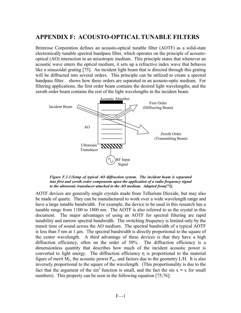
F—1

APPENDIX F: ACOUSTO-OPTICAL TUNABLE FILTERS Brimrose Corporation defines an acousto-optical tunable filter (AOTF) as a solid-state electronically tunable spectral bandpass filter, which operates on the principle of acousto-optical (AO) interaction in an anisotropic medium. This principle states that whenever an acoustic wave enters the optical medium, it sets up a refractive index wave that behaves like a sinusoidal grating [75]. An incident light beam that is directed through this grating will be diffracted into several orders. This principle can be utilized to create a spectral bandpass filter. shows how these orders are separated in an acousto-optic medium. For filtering applications, the first order beam contains the desired light wavelengths, and the zeroth order beam contains the rest of the light wavelengths in the incident beam.

Figure F.1.1:Setup of typical AO diffraction system. The incident beam is separated into first and zeroth order components upon the application of a radio frequency signal to the ultrasonic transducer attached to the AO medium. Adapted from[75].

AOTF devices are generally single crystals made from Tellurium Dioxide, but may also be made of quartz. They can be manufactured to work over a wide wavelength range and have a large tunable bandwidth. For example, the device to be used in this research has a tunable range from 1100 to 1800 nm. The AOTF is also referred to as the crystal in this document. The major advantages of using an AOTF for spectral filtering are rapid tunability and narrow spectral bandwidth. The switching frequency is limited only by the transit time of sound across the AO medium. The spectral bandwidth of a typical AOTF is less than 5 nm at 1 µm. The spectral bandwidth is directly proportional to the square of the center wavelength. A third advantage of these devices is that they have a high diffraction efficiency, often on the order of 50%. The diffraction efficiency is a dimensionless quantity that describes how much of the incident acoustic power is converted to light energy. The diffraction efficiency η is proportional to the material figure of merit M2, the acoustic power Pac, and factors due to the geometry L/H. It is also inversely proportional to the square of the wavelength. (This proportionality is due to the fact that the argument of the sin2 function is small, and the fact the sin x ≈ x for small numbers). This property can be seen in the following equation [75;76]:

Incident Beam

RF InputSignal

First Order (Diffracting Beam)

Zeroth Order (Transmitting Beam)

Ultrasonic Transducer

AO

Acoustic Absorber

F—2

⋅⋅⋅⋅⋅⋅⋅⋅⋅⋅⋅⋅====

HLPM ac

2sin 22

λλλλππππηηηη ( F.1 )

Geometric considerations are important when designing a system containing an AOTF. The first and zeroth order beams generally diverge at angles of approximately 5°. A beam cutter is generally inserted into the optical path at a distance from the output of the device in order to block the zeroth order beam. The closer this cutter is placed to the device, the more accurate the placement must be, or stray light from the zeroth order beam will leak into the optical path. There are two additional requirements for using an AOTF. The first is that light entering the device must be polarized. This ensures that the phase matching condition is necessary for proper operation of the device. (The phase matching condition involves the way that the sound and light waves interact in the crystal to implement a bandpass filter.) A second polarizer is placed after the AOTF, at right angles to the first. The second polarizer is used to help decrease the stray light in the optical path. The last requirement is that the focused light that is incident on the device may enter at a maximum angle of five to seven degrees [75].