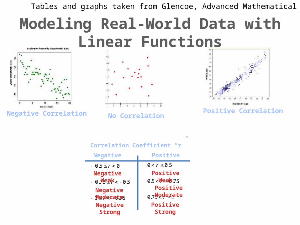
Modeling Real-World Data with Linear Functions

Positive CorrelationNegative Correlation No Correlation

Tables and graphs taken from Glencoe, Advanced Mathematical Concepts

Correlation Coefficient “r”

175.0

75.05.0

5.00

r

r

r

75.01

5.075.0

05.0

r

r

r

PositiveNegative

Positive Weak

Positive Moderate

Positive Strong

Negative Weak

Negative Moderate

Negative Strong

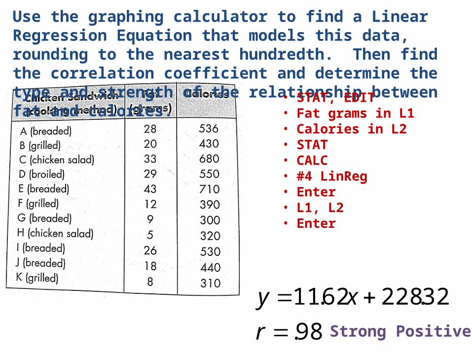
Use the graphing calculator to find a Linear Regression Equation that models this data, rounding to the nearest hundredth. Then find the correlation coefficient and determine the type and strength of the relationship between fat and calories.

• STAT, EDIT• Fat grams in L1• Calories in L2• STAT• CALC• #4 LinReg• Enter• L1, L2• Enter

98.

32.22862.11

r

xyStrong Positive

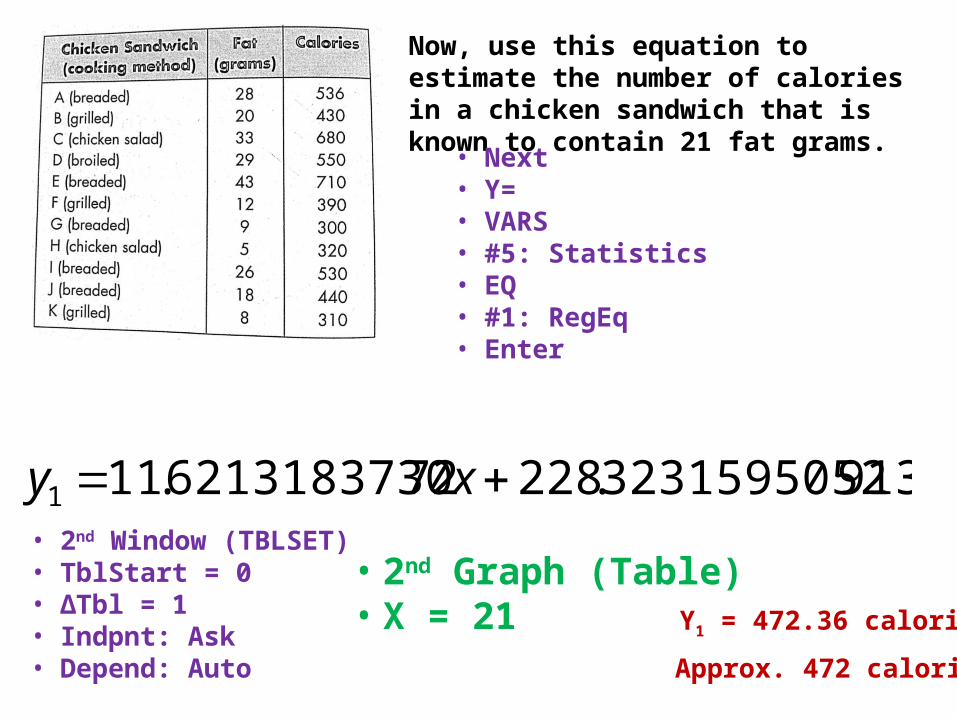
Now, use this equation to estimate the number of calories in a chicken sandwich that is known to contain 21 fat grams.

Approx. 472 calories

• Next• Y=• VARS• #5: Statistics• EQ• #1: RegEq• Enter

9133231595052.228726213183730.111 xy• 2nd Window (TBLSET)• TblStart = 0• ∆Tbl = 1• Indpnt: Ask• Depend: Auto

• 2nd Graph (Table)• X = 21 Y1 = 472.36 calories

Use the equation to estimate the number of fat grams in a food with 400 calories.

Approx. 15 fat grams

9133231595052.228726213183730.111 xy

9133231595052.228726213183730.11400 x

x

x

77257872.14

726213183730.116768405.171

Use the graphing calculator to find a Linear Regression Equation that models this data, rounding to the nearest hundredth. Then find the correlation coefficient and determine the type and strength of the relationship between year and average number of students. Let x = 3 represent the school year 1983-1984.

82.0

70.9228.6

r

xyStrong Negative

Now, use this equation to estimate the average number of students per computer in the academic year 1995-1996. Does this prediction seem reasonable?

-1.5, NO

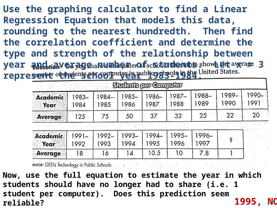
Use the graphing calculator to find a Linear Regression Equation that models this data, rounding to the nearest hundredth. Then find the correlation coefficient and determine the type and strength of the relationship between year and average number of students. Let x = 3 represent the school year 1983-1984.

Now, use the full equation to estimate the year in which students should have no longer had to share (i.e. 1 student per computer). Does this prediction seem reliable?

1995, NO

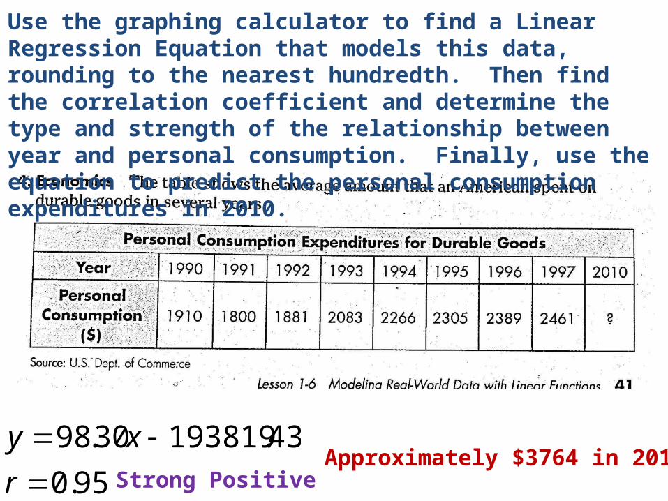
Use the graphing calculator to find a Linear Regression Equation that models this data, rounding to the nearest hundredth. Then find the correlation coefficient and determine the type and strength of the relationship between year and personal consumption. Finally, use the equation to predict the personal consumption expenditures in 2010.

95.0

43.19381930.98

r

xyStrong Positive

Approximately $3764 in 2010

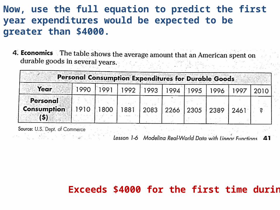
Now, use the full equation to predict the first year expenditures would be expected to be greater than $4000.

Exceeds $4000 for the first time during 2012

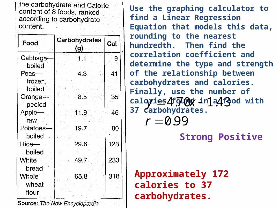
Use the graphing calculator to find a Linear Regression Equation that models this data, rounding to the nearest hundredth. Then find the correlation coefficient and determine the type and strength of the relationship between carbohydrates and calories. Finally, use the number of calories found in a food with 37 carbohydrates.

99.0

43.170.4

r

xy

Strong Positive

Approximately 172 calories to 37 carbohydrates.

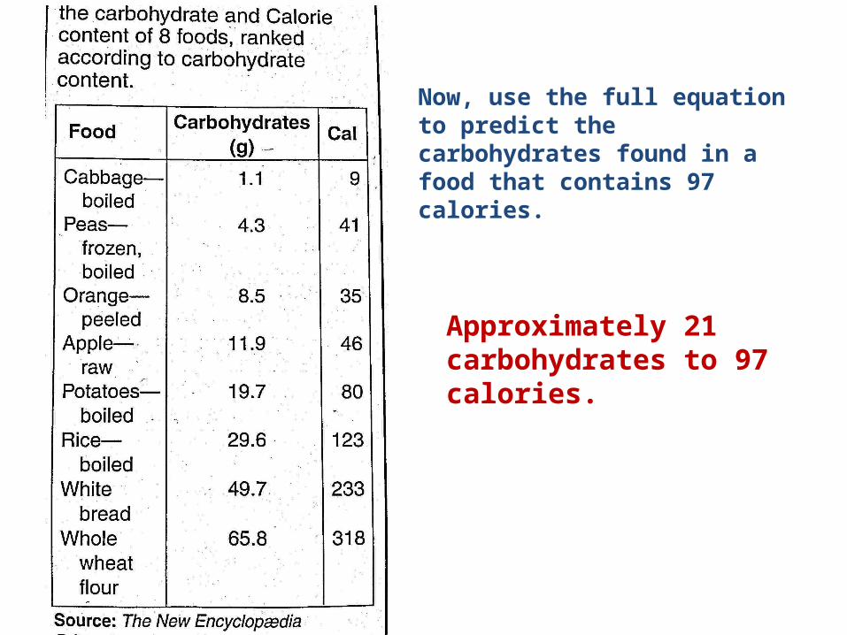
Now, use the full equation to predict the carbohydrates found in a food that contains 97 calories.

Approximately 21 carbohydrates to 97 calories.

Use the graphing calculator to find a Linear Regression Equation that models this data, rounding to the nearest hundredth. Then find the correlation coefficient and determine the type and strength of the relationship between year and personal income. Finally, use the equation to predict the personal income in 2005, and to determine the year that personal income would be expected to first exceed $45,000.

99.

64.207612932.1052

r

xy

Strong Positive

Approximately $33,772 in 2005

Exceeds $45,000 in 2016

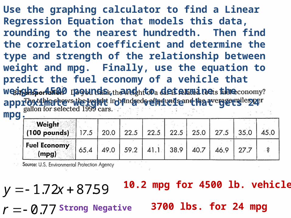
Use the graphing calculator to find a Linear Regression Equation that models this data, rounding to the nearest hundredth. Then find the correlation coefficient and determine the type and strength of the relationship between weight and mpg. Finally, use the equation to predict the fuel economy of a vehicle that weighs 4500 pounds, and to determine the approximate weight of a vehicle that gets 24 mpg.

77.0

59.8772.1

r

xyStrong Negative

10.2 mpg for 4500 lb. vehicle

3700 lbs. for 24 mpg

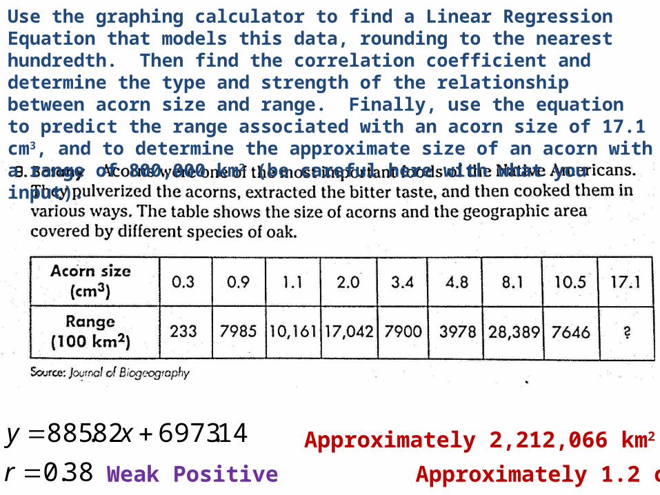
Use the graphing calculator to find a Linear Regression Equation that models this data, rounding to the nearest hundredth. Then find the correlation coefficient and determine the type and strength of the relationship between acorn size and range. Finally, use the equation to predict the range associated with an acorn size of 17.1 cm3, and to determine the approximate size of an acorn with a range of 800,000 km2 (be careful here with what you input).

38.0

14.697382.885

r

xy

Weak Positive

Approximately 2,212,066 km2

Approximately 1.2 cm3

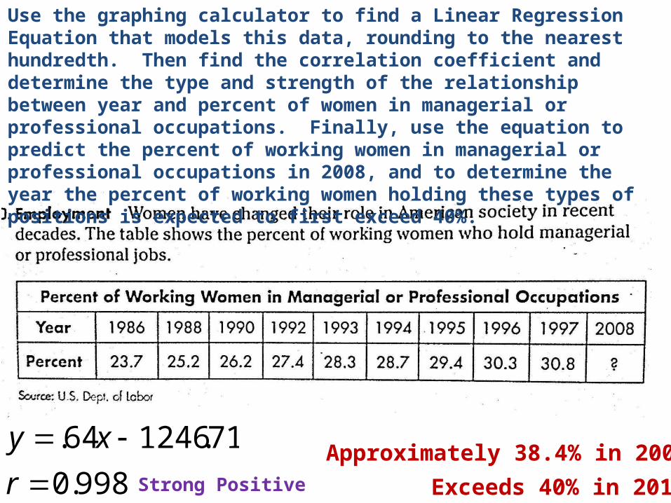
Use the graphing calculator to find a Linear Regression Equation that models this data, rounding to the nearest hundredth. Then find the correlation coefficient and determine the type and strength of the relationship between year and percent of women in managerial or professional occupations. Finally, use the equation to predict the percent of working women in managerial or professional occupations in 2008, and to determine the year the percent of working women holding these types of positions is expected to first exceed 40%.

998.0

71.124664.

r

xy Approximately 38.4% in 2008

Exceeds 40% in 2010.Strong Positive

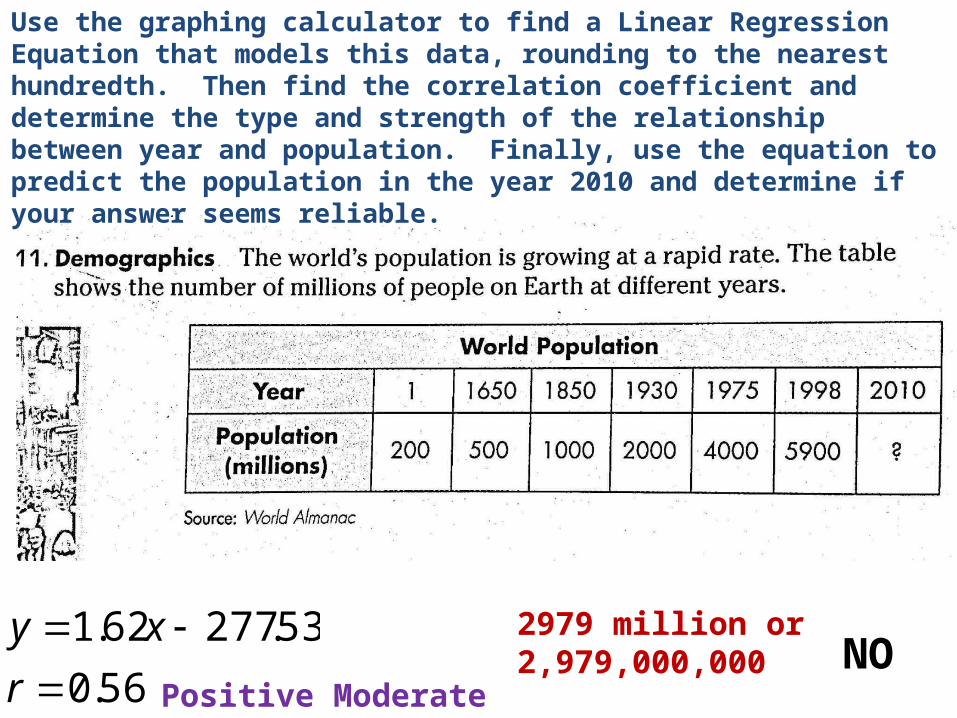
Use the graphing calculator to find a Linear Regression Equation that models this data, rounding to the nearest hundredth. Then find the correlation coefficient and determine the type and strength of the relationship between year and population. Finally, use the equation to predict the population in the year 2010 and determine if your answer seems reliable.

56.0

53.27762.1

r

xy

Positive Moderate

2979 million or2,979,000,000 NO

98.0

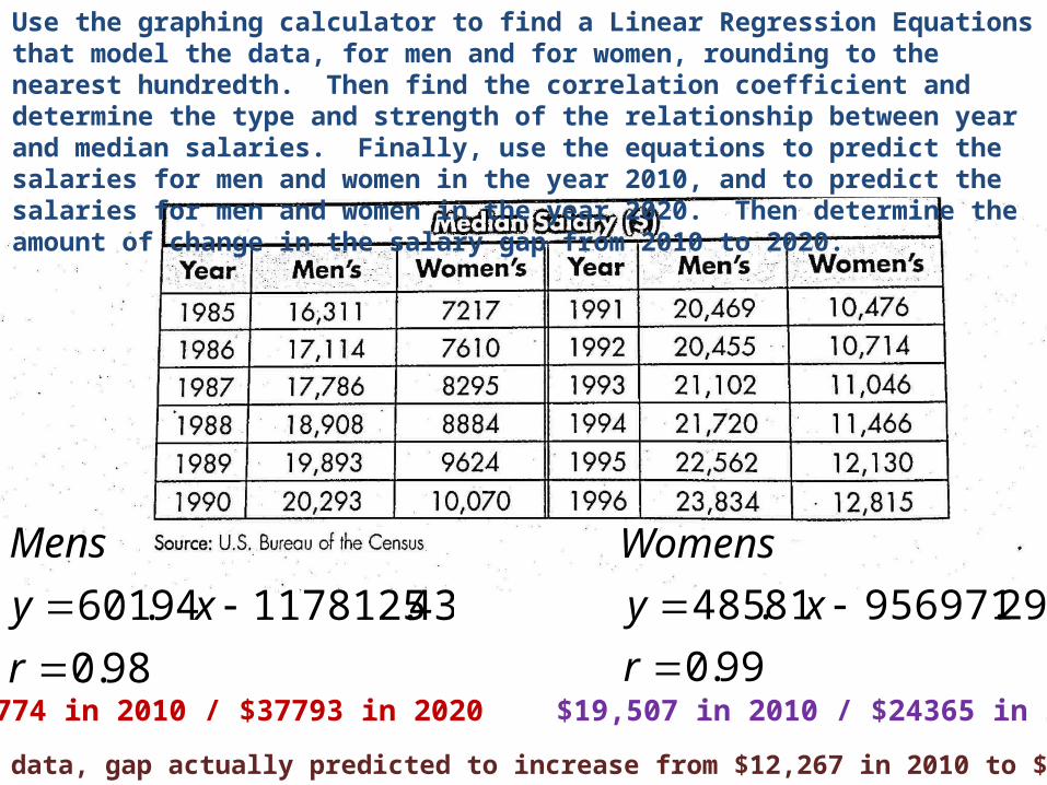
43.117812594.601

r

xy

Mens

99.0

29.95697181.485

r

xy

Womens

Use the graphing calculator to find a Linear Regression Equations that model the data, for men and for women, rounding to the nearest hundredth. Then find the correlation coefficient and determine the type and strength of the relationship between year and median salaries. Finally, use the equations to predict the salaries for men and women in the year 2010, and to predict the salaries for men and women in the year 2020. Then determine the amount of change in the salary gap from 2010 to 2020.

$31774 in 2010 / $37793 in 2020 $19,507 in 2010 / $24365 in 2020

Based on this data, gap actually predicted to increase from $12,267 in 2010 to $13,428 in 2020.