tcrreview1 - university of waterloo

p

Proceedings of HTC’03ASME Summer Heat Transfer ConferenceJuly 21-23, 2003, Las Vegas, Nevada, USA

HT2003-47051

REVIEW OF THERMAL JOINT RESISTANCE MODELS FOR NON-CONFORMINGROUGH SURFACES IN A VACUUM

Bahrami M.1, Culham J. R.2, Yovanovich M. M.3, and Schneider G. E.4

Microelectronics Heat Transfer Laboratory,Department of Mechanical Engineering,

University of Waterloo, Waterloo, Ontario, Canada

ABSTRACTThe thermal contact resistance (TCR) problem is catego-

rized into three different problems: geometrical, mechanical, andthermal. Each problem includes a macro and micro scale sub-problem; existing theories and models for each part are reviewed.

Empirical correlations for microhardness, and the equivalent(sum) rough surface approximation are discussed. Suggestedcorrelations for estimating the mean absolute surface slope aresummarized and compared with experimental data.

The classical conforming rough contact models, i.e elasticand plastic, as well as elastoplastic models are reviewed. A setof scale (dimensionless) relationships are derived for the contactparameters, i.e. the mean microcontact size, number of micro-contacts, density of microcontacts, and the external load as func-tions of dimensionless separation, for the above models. Thesescale relationships are plotted; it is graphically shown that thebehavior of these models, in terms of the contact parameters,are similar.

The most common assumptions of existing thermal analysisare summarized. As basic elements of thermal analysis, spread-ing resistance of a circular heat source on a half-space and fluxtube are reviewed, also existing flux tube correlations are com-pared.

More than 400 TCR data points collected by different re-searchers during last forty years are grouped into two limitingcases: conforming rough, and elasto-constriction. Existing TCRmodels are reviewed and compared with the experimental dataat these two limits. It is shown that the existing theoreticalmodels do not cover both of the above-mentioned limiting cases.

1Ph.D. Candidate, Department of Mechanical Engineering.2Associate Professor, Director, Microelectronics Heat Transfer Lab-

oratory. member ASME .3Distinguished Professor Emeritus, Department of Mechanical En-

gineering. Fellow ASME.4Professor, Department of Mechanical Engineering.

NOMENCLATUREA = area, m2

a = radius of contact, mb = flux tube radius, mc1, c2 = microhardness coefficients, GPa,−d = mean plane separation, GW modeldV = Vickers indentation diagonal, µmE = Young’s modulus, GPaE0 = equivalent elastic modulus, GPaF = external force, NH,HB = bulk hardness, GPaHmic = microhardness, GPaHBGM = geometric mean Brinell hardness, GPah = thermal contact conductance, W/m2Kk = thermal conductivity, W/mK

ks =harmonic mean thermalconductivity,W/mK

L = sampling length, mm = effective mean absolute surface slope, −m0 = effective RMS surface slope, −ns = number of microcontactsP = pressure, PaQ = heat flow rate, Wq = heat flux, W/m2

R = thermal contact resistance, K/WRMS = root mean squareRa = arithmetic average surface roughness, µmRq = RMS surface roughness, µmT = temperature, KY = mean surface plane separation, m

1 Copyright c° 2003 by ASME

Greekβ = summits radii of curvature, mγ = plasticity indexδ = surface max out-of-flatness, mε = flux tube relative radiusη = microcontact densityκ = HB/HBGMλ = dimensonless separationν = Poisson’s ratioφ = normal probability functionψ = dimensionless spreading resistanceρ = radius of curvature, mσ = RMS surface roughness, µmω = normal deformation, mξ = emprical correction factor

Subscripts0 = value at origin1, 2 = surface 1, 2a = apparentb = bulkc = conduction, contacte = effectiveg = gapGW = Greenwood and WilliamsonHz = Hertzj = jointL = large (macro scale)m = meanmac = macromic = micror = reals = smallV = Vickers

INTRODUCTION

Heat transfer through interfaces formed by the mechan-ical contact of two non-conforming rough solids, occurs in awide range of applications, such as: microelectronic cool-ing, spacecraft structures, satellite bolted joints, nuclearengineering, ball bearings, and heat exchangers. Analyti-cal, experimental, and numerical models have been devel-oped to predict thermal contact resistance since the 1930’s.The number of publications on thermal contact resistanceamounts to several hundred papers, which illustrates theimportance of this issue, and also indicates that the de-velopment of a general predictive model is a difficult task.Generally, contact between two surfaces occurs only overmicroscopic contacts. The real area of contact, the totalarea of all microcontacts, is typically a small fraction of

T

ZDT

T1

T2

temperature profile

microcontacts constriction

body 1

body 2

macro constriction resistance

Q

Q

F

F

aL

Qi

Q = S Qi

Figure 1. Macro and micro thermal constriction/spreading resistances

the nominal contact area [1,2]. As illustrated in Fig.1, themacroscopic contact region arises due to out-of-flatness ofbodies; and the microcontacts form due to interface be-tween contacting asperities of rough surfaces. In these sit-uations heat flow experiences two stages of resistance inseries, macroscopic and microscopic constriction resistance[3-5]. This phenomenon leads to a relatively high tempera-ture drop across the interface.

Thermal energy can be transferred between contactingbodies by three different modes, i) conduction at the mi-crocontact spot, ii) conduction through the interstitial fluidin the gap between the contacting solids, and iii) thermalradiation across the gap. The radiation heat transfer re-mains small and can be neglected for surface temperaturesup to 700 K [3,6]. Since in this study the interstitial fluidis assumed to be absent, the only remaining heat transfermode is conduction at the microcontacts.

Thermal contact resistance (TCR) problems basicallyconsist of three different problems: geometrical, mechani-cal, and thermal. Figure 2 illustrates the thermal contactresistance problem flow diagram and its components. Theheart of a TCR analysis is its mechanical part. Any solu-tion for the mechanical problem requires that the geometryof the contacting surfaces (macro and micro) be quantita-tively described. The mechanical problem also includes twoparts: macro or large-scale contact and micro or small-scalecontact. The mechanical analysis determines the macro-contact radius, aL, and the pressure distribution for thelarge-scale problem. For the microcontact problem separa-


Geometrical Analysis

Macro-Geometry Micro-Geometry

Macro-Contact(Bulk Deformations)

Mechanical Analysis

Micro-Contacts(Asperity Deformations)

Coupled

Macro-Constriction

Thermal Analysis

Micro-Constriction

Thermal Joint Resistance

Superposition

Resistance Resistance

Figure 2. Thermal contact resistance modeling flow diagram

tion between the mean contacting planes, microcontact size,density of microcontacts, and the relative microcontact ra-dius are calculated. The macro and the micro mechanicalproblems are coupled. The thermal analysis, based on theresults of the mechanical analysis, is then used to calculatethe microscopic and macroscopic thermal resistances.

GEOMETRICAL ANALYSIS

It is necessary to consider the effect of both sur-face roughness and out-of-flatness on the contact of non-conforming rough surfaces. Therefore, the geometrical anal-ysis is divided into micro and macro parts.

Micro Geometrical Analysis

All solid surfaces are rough, this roughness or surfacetexture, can be thought of as the surface deviation from thenominal topography. Surface textures can be created usingmany different processes. Most man-made surfaces, such asthose produced by grinding or machining have a pronounced“lay”. Generally, the “Gaussian surface” term is used torefer to a surface, where its asperities are isotropic and ran-domly distributed over the surface. It is not easy to producea wholly isotropic roughness. The usual procedure for ex-perimental purposes is to air-blast a metal surface with acloud of fine particles, in the manner of shot peening, whichgives rise to a randomly created surface. According to Liu,et al. [8] five types of instruments are currently availablefor measuring the surface topography, namely: stylus-type

surface profilometer, optical (white-light interference) mea-surements, Scanning Electron Microscope (SEM), AtomicForce Microscope (AFM), and Scanning Tunneling Micro-scope (STM). Among these, the first two instruments areusually used for macro-to-macro asperity measurements,whereas the others may be used for micro or nanometricmeasurements. Surface texture is most commonly measuredby a profilometer, which draws a stylus over a sample lengthof the surface. A datum or centerline is established by find-ing the straight line (or circular arc in the case of roundcomponents) from which the mean square deviation is aminimum. The arithmetic average of the absolute values ofthe measured profile height deviations, Ra, taken within asampling length from the graphical centerline [9]. The valueof Ra is

Ra =1

L

Z L

0

|z (x)|dx (1)

where, L is the sampling length in the x direction and z isthe measured value of the surface height along this length.When the surface is Gaussian, the standard deviation σ isidentical to the RMS value, Rq

σ = Rq =

s1

L

Z L

0

z2 (x) dx (2)

For a Gaussian surface, Ling [10] showed that the averageand RMS heights are related as follows

Rq ≈r

π

2Ra ≈ 1.25Ra (3)

Similarly, the absolute average and RMS asperity slopes, mand m0 respectively, can be determined across the samplinglength from the following

m =1

L

Z L

0

¯̄̄̄dz (x)

dx

¯̄̄̄dx, m0 =

s1

L

Z L

0

µdz (x)

dx

¶2dx(4)

Mikic and Rohsenow [4] showed that for Gaussian surfacesthe relationship between the average and RMS values of theasperity slopes ism0 ≈ 1.25m. Tanner and Fahoum [11] andAntonetti et al. [12], using published experimental surfacedata, suggested empirical correlations to relate RMS asper-ity slope, m0, to average roughness, Ra. Lambert [13], also


σ (µm)

m

10-1 100 10110-2

10-1

100

Tanner-Fahoum [11]Antonetti et al. [12]Lambert [13]Antonetti [59]Burde [48]Hegazy [24]McMillan- Mikic [63]Milanez et al. [60]

Figure 3. Comparison between correlations for m and experimental data

Table 1. Correlations for m, Gaussian surface

Reference Correlation

Tanner and Fahoum [11] m = 0.152 σ0.4

Antonetti et al. [12] m = 0.124 σ0.743, σ ≤ 1.6 (µm)

Lambert [13] m = 0.076 σ0.52

using the same method, correlated the absolute average as-perity slopes, m, as a function of RMS roughness (micron);correlations for m are summarized in Table 1. Figure 3illustrates the comparison between these correlations andexperimental data. As shown in Fig.3, the uncertainty ofthe above correlations is high, and use of these correlationsare justifiable only where the surface slope is not reportedand or a rough estimation of m is needed.

Equivalent (Sum) Rough Surface According to the ex-amination of the microgeometry with equivalent magnitudein the vertical direction and in the traversing direction,asperities seem to have curved shapes at their tops [14].A common assumption/methodology to model the surfaceroughness is the representation of surface asperities by sim-ple geometrical shapes with a probability distribution forthe different asperity parameters involved. One of the firstpresentations to use this asperity-based model is found inCoulomb’s work in 1782. To explain the laws of friction,he assumed that the asperities possessed a spherical shapeall of which had the same radius and the same summit al-titude. Greenwood and Williamson [1] assumed that each

asperity summit had a spherical shape whose height above areference plane had a normal (Gaussian) probability densityfunction. Williamson et al. [15] have shown experimentallythat many of the techniques used to produce engineeringsurfaces give a Gaussian distribution of surface heights.

The solution of any contact mechanics problem requiresthat the geometry of the intersection and overlap of the twoundeformed surfaces be known as a function of their relativeposition. Greenwood [16] stated that; “a genuine treatmentof two rough surfaces is complicated by the difficulty of de-scribing the unit event, the formation of a single contactspot. For example, if both surfaces are covered by spheres,it is necessary to study the contact of one sphere on theshoulder of another, and then evaluate the probabilities ofdifferent degrees of misalignment, in order to get the aver-age unit event. A non-genuine treatment is comparativelysimple: both surfaces are taken to be rough with normal dis-tributions. The statistical treatment now concerns the prob-ability of the sum of two heights (which is also normally dis-tributed) exceeding the separation, and this is exactly equiv-alent to a distribution of a single variable.” In other words,the contact between Gaussian rough surfaces can be con-sidered as the contact between a single Gaussian surface,having the effective (sum) surface characteristics, placed incontact with a perfectly smooth flat surface. Also, since theslope, m, of a profile is proportional to the difference be-tween adjacent equispaced ordinates; m is Gaussian if theprofile is Gaussian [17]. This simplification was used bymany researchers, such as: Clausing and Chao [3], Cooperet al. [18], Francis [19], and Johnson [7]. The equivalentroughness and surface slope can be calculated from

σ =qσ21 + σ22 and m =

qm21 +m

22 (5)

According to Francis [19], a contact model based on thesum (equivalent) surface circumvents the problem of mis-alignment of contacting peaks; in addition, the sum surfacesees peak to valley and peak to saddle contacts. The sumsurface of two Gaussian surfaces is itself Gaussian and ifparent surfaces are not exactly Gaussian, the sum (equiv-alent) surface will be closer to Gaussian than the parentsurfaces. Additionally, the sum surface will be in generalless anisotropic than the two contacting surfaces, thus theGaussian sum surface is a reasonable basis for a general con-tact model [19]. Figure 4 shows a normal section throughthe contact in which the surfaces are imagined to overlapwithout deforming, and the equivalent rough or sum sur-face of the contact in the same normal section. The overlapgeometry as a function of the mean separation, Y, of theundeformed surfaces is thus given directly and exactly bythe shape of the equivalent rough surface. The number of


σY

mω z

ω

Y zzmm

σσ

smooth flat

mean plane 2

mean plane 1

plane1 1 1

22 2

b) Corresponding section through equivalent rough - smooth flat

a) Section through two contacting surfaces

Figure 4. Equivalent contact of conforming rough surfaces

microcontacts, which have formed, is simply the number ofequivalent surface peaks that have; Z ≥ Y .

Macro Geometrical Analysis

Many studies on thermal contact resistance ideally as-sume a uniform distribution of micro contact spots, i.e. con-forming rough surface models. Such approaches are success-ful, where the macroscopic nonuniformity of the contact isnegligible. However, no real engineering surfaces are per-fectly flat, thus the influence of macroscopic nonuniformitycan never be ignored. Considering the waviness or out-of-flatness of contacting surfaces in a comprehensive manner isvery complex because of the case-by-case nature of the wavi-ness. Certain simplifications must be introduced to describethe macroscopic topography of surfaces by a few parame-ters. A sphere is the simplest example of a macroscopicallyhomogenous surface. Specifically, its profile is describedonly by its radius. Theoretical approaches by Clausing andChao [20], Mikic and Rohsenow [4], Yovanovich [5], Nishinoet al. [21], and Lambert and Fletcher [22] assumed that aspherical profile may approximate the shape of the macro-scopic nonuniformity. According to Lambert [13] this as-sumption is justifiable, because nominally flat engineeringsurfaces are often spherical, or crowned (convex) with amonotonic curvature in at least one direction.

According to Johnson [7], in static frictionless contactof solids, the contact stresses depend only upon the rela-tive profile of the two surfaces, i.e. upon the shape of theinterstitial gap between them before loading. The actualsystem geometry may be replaced, without loss of general-ity, by a flat surface and a profile, which results in the sameundeformed gap between the surfaces. For convenience, allelastic deformations can be considered to occur in one body,which has an effective elastic modulus and the other body

a) contact of non-conforming rough surfaces

b) contact of two rough spherical segments

c) rough sphere-flat contact, effective radius of curvature

ρ

σeffective radius and roughness

ρ

ρ

ρ

L

d1

2

σσ1

2

Lb

Figure 5. Flow diagram of geometrical modeling

is assumed to be rigid. The effective elastic modulus can befound from

1

E0=1− υ21E1

+1− υ22E2

(6)

where, E and υ are the Young’s modulus and Poisson’sratio, respectively. For the contact of two spheres, the ef-fective radius of curvature is:

1

ρ=1

ρ1+1

ρ2(7)

The relation between radius of curvature and the maximumout-of-flatness is [3]

ρ =b2L2δ

(8)

where, δ is the maximum out-of-flatness of the surface.Figure 5 details the procedure, which has been used

widely for the geometric modeling of the actual contact be-tween two curved rough bodies. As the result of the above,the complex geometry of non-conforming rough contactscan be simplified to the contact of the equivalent truncatedspherical surface with the equivalent rough flat.

Microhardness

Hardness is defined as the resistance to permanent de-formation; hardness definitions and tests can be found invarious standard textbooks e.g. Tabor [2], and Mott [23].The most common hardness testing method is the staticindentation. In a static indentation test, a steady load


** *

** *

* *

Indentation depth t (µm)

Har

dnes

sH

(GPa

)

100 101 102 1031

1.5

2

2.5

3

3.5

4

SS 304Ni 200Zr-2.5% wt NbZr-4

*

macro-hardnessVickers micro-hardness

tdV

dV / t = 7

Figure 6. Measured hardness and microhardness, Hegazy [24]

is applied to an indenter which may be a ball, cone orpyramid and the hardness is calculated from the area ordepth of indentation produced. Hegazy [24] demonstratedthrough experiments with four alloys, SS 304, nickel 200,zirconium-2.5% niobium, and Zircaloy-4, that the effectivemicrohardness is significantly greater than the bulk hard-ness. As shown in Fig.6, microhardness decreases with in-creasing depth of the indenter until bulk hardness is ob-tained. Hegazy concluded that this increase in the plasticyield stress (microhardness) of the metals near the free sur-face is a result of local extreme work hardening or some sur-face strengthening mechanism. He derived empirical corre-lations to account for the decrease in contact microhardnessof the softer surface with increasing depth of penetration ofasperities on the harder surface

Hv = c1 (d0v)c2 (9)

where, Hv is Vickers microhardness in (GPa), d0v = dv/d0

and d0 = 1 (µm), dv is Vickers indentation diagonal in(µm), and c1, c2 are correlation coefficients determined fromexperimental measurements. Table 2 shows c1 and c2 forsome materials. Relating the hardness of a microcontactto the mean size of microcontacts, Hegazy [24] suggesteda correlation for effective microhardness (conforming roughsurfaces)

Hmic = c1

µ0.95

σ0

m

¶c2(10)

where, σ0 = σ/σ0 and σ0 = 1 (µm) , σ is surface roughnessin micrometers. Microhardness depends on several parame-

Table 2. Vickers microhardness coefficients, Hegazy [24]

Material c1(GPa) c2

Zr-4 5.677 -0.278

Zr-2.5wt% Nb 5.884 -0.267

Ni 200 6.304 -0.264

SS 304 6.271 -0.229

ters: mean surface roughness, mean absolute slope of asper-ities, method of surface preparation, and applied pressure.Song and Yovanovich [25] related Hmic to the surface pa-rameters and nominal pressure (conforming rough surface)

P

Hmic=

·P

c1 (1.62σ0/m)c2

¸1/(1+0.071c2)(11)

Sridhar [26] suggested empirical relations to estimate Vick-ers microhardness coefficients, using the bulk hardness ofthe material. Two least-square-cubic fit expressions werereported

c1 = HBGM¡4.0− 5.77κ+ 4.0κ2 − 0.61κ3¢

c2 = −0.57 + 0.82κ− 0.41κ2 + 0.06κ3 (12)

where, κ = HB/HBGM , HB is the Brinell hardness of thebulk material, and HBGM = 3.178(GPa). The above cor-relations are valid for the range 1.3 ≤ HB ≤ 7.6 (GPa)with the RMS percent difference between data and calcu-lated values were reported; 5.3% and 20.8% for c1, and c2,respectively.

MECHANICAL ANALYSIS

Figure 7 illustrates the mechanical analysis overview forcontact of spherical rough surfaces, which includes; a macroand a micro part. Existing theories/models for each part(macro and micro) is categorized based on the normal de-formation mode of the bulk (substrate) and asperities into:elastic, plastic, and elastoplastic groups.

Macrocontact Problem

When two smooth solid spheres, or equivalently a flatand the effective sphere, are pressed against each other, withincrease in external load, the three ranges of loading: purelyelastic, elastic-plastic (contained) and fully plastic (uncon-tained) occur in the most engineering structures. Hertz


ρO

F

O

ρ

F

elastic half-space

Elasticity theoryElastoplastic deformationFully plastic deformation

contact plane

σ

smooth flat

m

ωY Z

plane

Plastic Elastic Elastoplastic models

a

a

P(r) σ

contact of spherical rough surfaces

smooth (Hertzian) contact (macro-scale)

contact of conforming rough surfaces (micro-scale)

contact plane elastic half-space

Hz

L

Figure 7. Mechanical problem overview for spherical rough contacts

[27] developed his elastic contact theory by introducing thesimplification that each body can be regarded as an elastichalf-space loaded over a small contact region of its planesurface. He also assumed surfaces are continuous and non-conforming, strains are small (to be in the elastic limit),surfaces are frictionless, and the pressure distribution is

P (r) = P0

q1− (r/aHz)2. The Hertz theory expressions,

can be summarized as

aHz =

µ3Fρ

4E0

¶1/3ω0 =

a2Hzρ=

µ9F 2

16ρE02

¶1/3(13)

P0 =3F

2πa2Hz=

Ã6FE0

2

π3ρ2

!1/3

where, ω0 is the maximum deformation, and P0 is the max-imum pressure (at the center of the contact).

According to Johnson [7], the load at which plastic yieldbegins in the contact of two solids, is related to the yieldpoint of the softer material. The yield point can be foundeither from Tresca’s maximum shear stress, or Von Mises’shear strain-energy criterion. When the yield point is firstexceeded the plastic zone is small and fully contained bymaterial which remains elastic so that the plastic strainsare of the same order of magnitude as the surrounding elas-tic strains. In these circumstances the material displacedby the indenter, is accommodated by an elastic expansionof the surrounding solid. As the indentation becomes more

severe, the plastic zone (core) expands, and an increasingpressure is required beneath the indenter to produce thenecessary expansion. Eventually the plastic zone breaksout to the free surface and displaced material is free to es-cape by plastic flow to the sides of the indenter. This isthe uncontained mode of deformation, which should be an-alyzed by the theory of rigid-plastic solids [7]. However,the contact load must be increased about 400 times fromthe point of initial yielding to the state of fully plastic flow,which indicates that the elastoplastic transitional region isvery long.

When the plastic deformation is severe so that the plas-tic strains are large compared with the elastic strains, theelastic deformation may be neglected. Provided the ma-terial does not strain-harden to a large extent, it may beidealized as a perfectly plastic solid, which flows plasticallyat a constant stress (roughly three times the yield stress)[7]. A loaded body of rigid-plastic material consists of re-gions in which, plastic flow takes place and regions in wherethere is no deformation due to the assumption of rigidity.Hardy et al. [28], using a numerical analysis, showed thatthe plastic flow leads to a flattening of the pressure distribu-tion and at high loads may peak slightly towards the edgeof the contact area.

Microcontact Problem

Based on the assumed deformation mode of asperities,existing microcontact mechanical models can be categorizedinto three main groups: plastic, elastic, and elastoplasticmodels. The fundamental assumptions, which are commonin most of the models can be summarized as

• contacting surfaces are rough, isotropic, with a Gaus-sian asperity distribution

• behavior of a given microcontact is independent of allother microcontacts

• interfacial force on any microcontact spot acts normally(no friction)

• the deformation mechanics (i.e. the stress and displace-ment fields) are uniquely determined by the shape of theequivalent surface.

Plastic Models Abott and Firestone [29] developed themost widely used model for a fully plastic contact. With theconcept of equivalent roughness, the model assumes that theasperities are flattened or, equivalently penetrate into thesmooth surface without any change in the shape of the partof surfaces not yet in contact. Therefore, bringing the twosurfaces together within a distance Y is equivalent to slicingoff the top of the asperities at a height Y above the meanplane. Since the true area of contact is much smaller than


the apparent contact area, the pressure at the top of the as-perities must be sufficiently large that they are comparablewith the strength of the materials of the contacting bodies.Bowden and Tabor [30], and Holm [31] suggested that thesecontact pressures are equal to the flow pressure of the softerof the two contacting materials and the normal load is thensupported by plastic flow of its asperities. Therefore, pres-sure at microcontacts will be equal to the microhardnessand effectively independent of load and the contact geom-etry. The true area of contact is then proportional to theload, Ar/Aa = Pm/Hmic, where Pm is the mean apparentcontact pressure.

Pullen and Williamson [32] experimentally investigatedplastic flow under large loads. They assumed that mate-rial displaced from the contacting regions must reappear byraising some part of the non-contacting surface. They as-sumed that the volume of material remained constant andthat the material that is plastically displaced appears as auniform rise over the entire surface. Since the uniform risewill not affect the shape of the surface outside the contactarea, they showed that the contact area due to the interac-tion of micro contacts is not proportional to the normal load(at relatively high loads); and proposed as a good approx-imation; Ar/Aa = Pp/ (1+ Pp) , where Pp = Pm/Hmic.Note that this phenomenon is important only at relativelylarge pressures.

Some authors used conical or curved shapes to de-scribe the morphology of asperities. Tsukizoe and Kisakado[33,34], assumed a conical shape for surface asperities ofequal base angle, which depends on the surface mean ab-solute slope. They proposed a statistical contact model forpredicting the contact spot size and density for an isotropicGaussian rough surface in contact with an ideal smooth flatsurface. On the basis of this assumption and neglecting theasperity interactions, they obtained the following expres-sions for microcontact size and number

as =√2π (σ/m) /λ

ns =√π8

¡mσ

¢2λ exp

¡−λ2¢Aa (14)

where, λ = Y/√2σ is the dimensionless separation.

Cooper et al.[18], based on the level-crossing theory andusing the sum surface approximation, derived relationshipsfor mean microcontact size, and number of microcontacts byassuming hemispherical asperities whose height and surfaceslopes have Gaussian distributions

as =q

8π (σ/m) exp

¡λ2¢erfc (λ)

ns =116Aa (m/σ)

2 exp¡−2λ2¢/erfc (λ) (15)

surface mean plane

mean summit height

separation

equivalent elastic rough surface

rigid smooth flat

z

β

z

d

Yβ

s

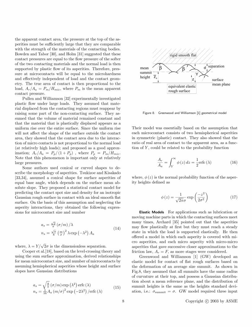
Figure 8. Greenwood and Williamson [1] geometrical model

Their model was essentially based on the assumption thateach microcontact consists of two hemispherical asperitiesin symmetric (plastic) contact. They also showed that theratio of real area of contact to the apparent area, as a func-tion of Y , could be related to the probability function

ArAa

=

Z ∞Y

φ (z) dz =1

2erfc (λ) (16)

where, φ (z) is the normal probability function of the asper-ity heights defined as

φ (z) =1√2πσ

exp

µ−z22σ2

¶(17)

Elastic Models For applications such as lubrication ormoving machine parts in which the contacting surfaces meetmany times, Archard [35] pointed out that the asperitiesmay flow plastically at first but they must reach a steadystate in which the load is supported elastically. He thenoffered a model in which each asperity is covered with mi-cro asperities, and each micro asperity with micro-microasperities that gave successive closer approximations to thefriction law, Ar = F, as more stages were considered.

Greenwood and Williamson [1] (GW) developed anelastic model for contact of flat rough surfaces based onthe deformation of an average size summit. As shown inFig.8, they assumed that all summits have the same radiusof curvature at their top, and possess a Gaussian distribu-tion about a mean reference plane, and the distribution ofsummit heights is the same as the heights standard devi-ation, i.e.: σsummit = σ. GW model required three input


parameters: the standard deviation of summit height distri-bution σsummit, the surface density of asperities ηGW , andthe radius of curvature of the summits β that was assumedto be constant. Relationships for the GW model, as re-ported, are

ns = ηGWAaI0 (d0)

Ar = πηGWAaβσI1 (d0) (18)

F =4

3ηGWAaβ

1/2σ3/2E0I3/2 (d0)

where, d0 = d/σ, and;

In (d0) =

1√2π

Z ∞d0(s− d0)n exp ¡−s2/2¢ ds

(19)

Unlike other models, the GW model is based on the con-tact of summits and separation, d, is measured from themean summit line (not the surface mean line), which is lo-cated somewhere above the mean surface plane. Since itwas assumed that the summits standard deviation is thesame as the surface roughness, the GW relationships can bere-written as functions of λ = Y/

√2σ (to make the rela-

tionships comparable with other models). After evaluatingthe integrals and simplifying, the relationships become

ns =1

2ηGWAaerfc (λ)

Ar =

√π

2ηGWAaβσ

£exp

¡−λ2¢−√πλ erfc (λ)¤ (20)F =

21/4

3√πηGWAaE

0β1/2σ3/2√λ exp

¡−λ2/ 2¢h¡1+ 2λ2

¢K 1

4

¡λ2/ 2

¢− 2λ2K 34

¡λ2/ 2

¢iwhere, Kn (.) is the modified Bessel function of the secondkind of the nth order.

The GW asperity model has been extended to includeother contact geometries, e.g. curved surfaces [36], morecomplex geometries, e.g. non-uniform radii of curvature ofasperity peaks [37], and anisotropic surfaces [38]. White-house and Archard [37] and Onions and Archard [39] fur-ther improved the statistic model by representing the fea-tures of the surface topography with two parameters: thestandard deviation, σ, and the exponent of an exponentialcorrelation function, which was named the “correlation dis-tance”. Bush et al. [40] developed an elastic contact modelfor isotropic surfaces that treated the asperities as ellipti-cal paraboloids with random principal axis orientation and

aspect ratio. O’Callaghan and Cameron [41] developed amodel for the isotropic problem addressed by Bush et al.[40]. In their model, both surfaces can be rough and as-perities need not contact at their tops. O’Callaghan andCameron [41] concluded, as did Francis [19], that the con-tact of two rough surfaces was negligibly different from thecontact of a smooth and an equivalent rough surface. Mc-Cool [42] compared the basic GW model with other moregeneral isotropic and anisotropic models and found that thesimpler GW model, despite its simplistic form, gives goodresults.

Elastoplastic Models Chang et al. [43], using GWmodel assumptions, presented a model based on volumeconservation of an asperity control volume during plasticdeformation. The deformed asperity was modeled as a trun-cated spherical segment and its radius was assumed to bethe same as that of the undeformed asperity. For all plasti-cally deformed asperities the average pressure over the con-tact area was assumed to be a factor of hardness, which wasconstant throughout the elastic-plastic deformation. Zhaoet al. [44], using the Chang et al. [43] model, developed anelastic-plastic microcontact model for nominally flat roughsurfaces. The transition from elastic deformation to fullyplastic flow of the contacting asperities was curve-fitted. Acubic polynomial, smoothly joining the expressions for elas-tic and plastic area of contacts spans the elastoplastic regionbased on two extremes of the Chang et al. [43] model.

The advantage of the GW-type models is their (rela-tive) simplicity and explicitness in expressions. However,assuming a constant summit radius is unrealistic; for a ran-dom surface, β is also a random variable [19]. In addition βand ηGW cannot be measured directly and must be calcu-lated through statistical relationships, and are sensitive tothe sampling length of the surface measurement [7].

Deformation Mode of Asperities When real surfaces arepressed together they make contact at numerous points,which deform, elastically, plastically or elastoplastically tosupport the load. According to Tabor [2] when two metalsare placed in contact “they will be supported on the tips oftheir asperities, at first the deformation is elastic, but forasperities of the order of µm radius, the minutest loads willproduce plastic deformation. Indeed full plasticity may oc-cur even for the hardest steels at a load of the order of a fewmilligrams.” Tabor showed that in most practical cases, thereal area of contact is proportional to the applied load. It isalso inversely proportional to the effective hardness of thesurface asperities. Greenwood [16] described the contact oftwo surfaces as: “surfaces touch at a large number of con-tacts, and these contacts will be in all the states from fully


elastic, to fully plastic. The fully elastic ones are a negli-gible fraction of the total; the effective flow pressure will beintermediate between plastic and elastic values.” Consider-ing the fact that the plastic flow is irreversible and cannotbe repeated on subsequent loadings, Archard [35] empha-sized the point that the normal contact must be elastic. Heshowed that any elastic model (based on simple Hertziantheory) in which the number of contacts remains constantwill give Ar ∼ F 2/3, which does not satisfy the observedproportionality Ar ∼ F reported by Tabor [2]. But, if theaverage contact size remains constant, and the number ofmicrocontact increases, the area will be proportional to theload.

Greenwood and Williamson [1] introduced a plastic-ity index as a criterion for plastic flow of microcontacts,γGW = (E0/H)

pσ/β. They reported that the load has

little effect on the deformation regime. When the indexis less than 0.6, plastic contact could be caused only if thesurfaces were forced together under very large nominal pres-sure. When γGW ≥ 1 plastic flow will occur even at smallnominal pressures. Based on the plasticity index, they con-cluded that; “most of surfaces have plasticity indices largerthan 1.0, and thus, except for especially smooth surfaces,the asperities will flow plastically under the lightest loads, ashas been frequently postulated.” Chang et al. [43] with thesame assumptions as GW, set the criteria for the deforma-tion mode based on the deformation of an average asperity.For compliances less than the critical compliance ωc, whereωc is the inception of plastic deformation based on exper-imental work of Tabor [2] and Johnson [7], the contact iselastic and Hertzian theory can be applied. For complianceshigher than ωc, a plastic model was used. Mikic [45] pro-posed an alternative plasticity index, γMikic = Hmic/E

0m.Mikic also reported that the mode of deformation, as statedby GW, depends only on material properties and the shapeof the asperities, and it is not sensitive to the pressure level.Mikic performed an analysis to determine the contact pres-sure over the contact area based on the fact that all contactspots do not have the same contact pressure, although theaverage contact pressure would remain constant. For sur-faces with γMikic ≥ 3, 90% of the actual area will havethe elastic contact pressure, therefore the contact will bepredominantly elastic, and for γMikic ≤ 0.33, 90% of theactual area will have the plastic contact pressure, thereforethe contact will be predominantly plastic. He concludedthat for most engineering surfaces the asperity deformationmode is plastic and the average asperity pressure is the ef-fective microhardness.

To compare elastic and plastic models, Greenwood andWilliamson [1] (GW) elastic, Cooper et al. [18] (CMY)plastic, and Tsukizoe and Kisakado [33, 34] (TK) plasticmodels were chosen, and their trends plotted vs. the di-

mensionless mean separation. GW requires input surfaceparameters; η, β and σ, while CMY and TK require σ, m,thus a quantitative comparison between these models re-quires detailed surface information, and would be restrictedto a particular case. However, for a contact, surface param-eters are constant and do not change as separation varies.Therefore, by considering surface parameters constant, scalerelationships derived and these models compared quantita-tively. This comparison only illustrates trend/behavior ofsurface parameters predicted by each model as the separa-tion changes.

Table 3 shows the scale relationships that were used inthe comparison. The real area of microcontacts was cal-culated from, Ar = πnsa

2s. Additionally, for CMY and TK

models, as the fully plastic deformation of asperities was as-sumed, the external force can be found from, F = HmicAr ,where microhardness (for a contact) considered a constant.

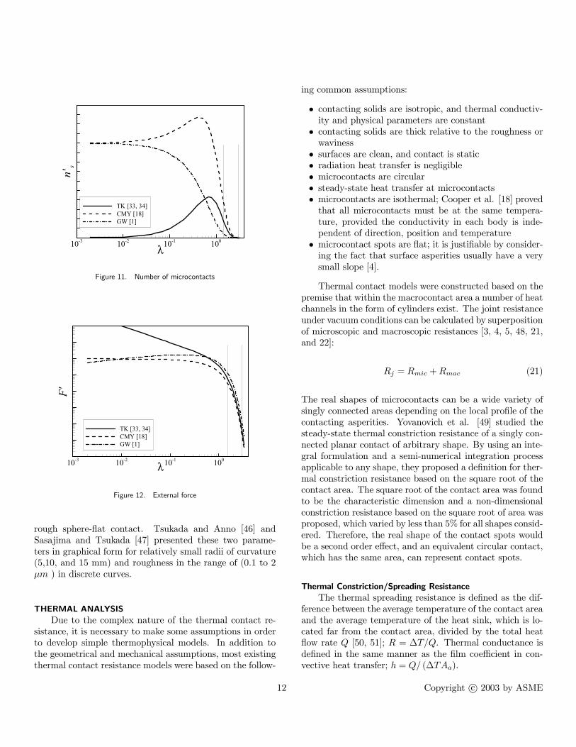
The range of separation in typical real contacts isroughly, 1.5 ≤ λ ≤ 3 . The (scale) relationships in Table3 are plotted versus the separation, λ, over a wider rangein Figs. 9 to 12. It can be observed that by decreasing theseparation;

• The mean size of microcontacts in all models increases.The size of microcontacts in the TK model increasescontinuously due to the assumed conical shape of as-perities, while the predicted mean microcontact size byGW and CMY approaches some limiting value.

• The real contact area increases and the trends predictedby the three models are very similar, in the applicablerange of the separation 1.5 ≤ λ ≤ 3.

• The external force also increases in a comparable man-ner in all three models. It is interesting to observe thatthe external force is (nearly) proportional to the realcontact area in GW model, which indicates that GW(elastic) model behaves similar to plastic models andan elastic effective microhardness can be defined.

• The number of microcontacts increases in CMY andTK to a maximum and falls by further decreasing theseparation, while the GW model does not show thisphenomena. As the separation becomes smaller, morecontacting spots form, also the mean size of the existingmicrocontact increases, until they begin to merge andcreate larger contact spots (clustering), which resultsin fewer microcontacts. Based on the microgeometrymodel, a rough surface can be imagined as a collectionof peaks and valleys. At the limit when separation ap-proaches zero, CMY and TK predict that all surfacepeaks (asperities higher than the mean line) are cutoff and only the ones under the mean line (valleys) re-main. On the other hand, the GW model predicts thatthe peaks are elastically compressed to the mean-line,


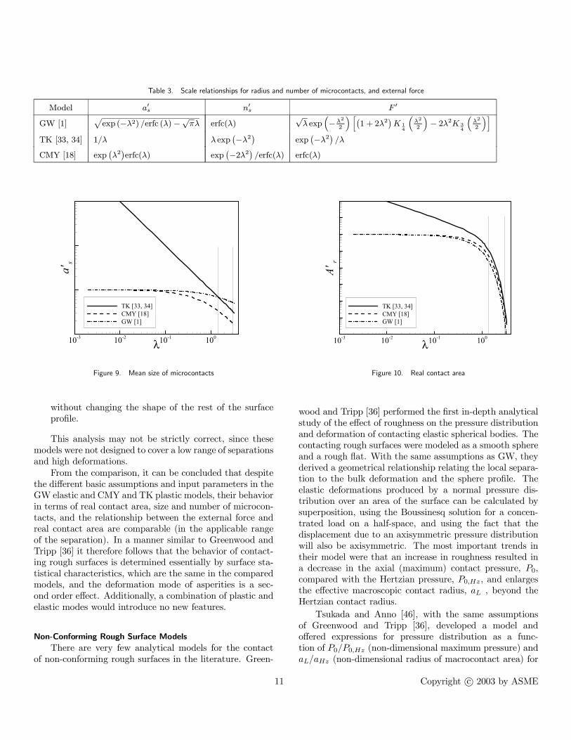
Table 3. Scale relationships for radius and number of microcontacts, and external force

Model a0s n0s F 0

GW [1]pexp (−λ2) /erfc (λ)−√πλ erfc(λ)

√λ exp

³−λ2

2

´ h¡1+ 2λ2

¢K 1

4

³λ2

2

´− 2λ2K 3

4

³λ2

2

´iTK [33, 34] 1/λ λ exp

¡−λ2¢ exp¡−λ2¢ /λ

CMY [18] exp¡λ2¢erfc(λ) exp

¡−2λ2¢ /erfc(λ) erfc(λ)

λ

a's

10-3 10-2 10-1 100

TK [33, 34]CMY [18]GW [1]

Figure 9. Mean size of microcontacts

without changing the shape of the rest of the surfaceprofile.

This analysis may not be strictly correct, since thesemodels were not designed to cover a low range of separationsand high deformations.

From the comparison, it can be concluded that despitethe different basic assumptions and input parameters in theGW elastic and CMY and TK plastic models, their behaviorin terms of real contact area, size and number of microcon-tacts, and the relationship between the external force andreal contact area are comparable (in the applicable rangeof the separation). In a manner similar to Greenwood andTripp [36] it therefore follows that the behavior of contact-ing rough surfaces is determined essentially by surface sta-tistical characteristics, which are the same in the comparedmodels, and the deformation mode of asperities is a sec-ond order effect. Additionally, a combination of plastic andelastic modes would introduce no new features.

Non-Conforming Rough Surface Models

There are very few analytical models for the contactof non-conforming rough surfaces in the literature. Green-

λA'

r10-3 10-2 10-1 100

TK [33, 34]CMY [18]GW [1]

Figure 10. Real contact area

wood and Tripp [36] performed the first in-depth analyticalstudy of the effect of roughness on the pressure distributionand deformation of contacting elastic spherical bodies. Thecontacting rough surfaces were modeled as a smooth sphereand a rough flat. With the same assumptions as GW, theyderived a geometrical relationship relating the local separa-tion to the bulk deformation and the sphere profile. Theelastic deformations produced by a normal pressure dis-tribution over an area of the surface can be calculated bysuperposition, using the Boussinesq solution for a concen-trated load on a half-space, and using the fact that thedisplacement due to an axisymmetric pressure distributionwill also be axisymmetric. The most important trends intheir model were that an increase in roughness resulted ina decrease in the axial (maximum) contact pressure, P0,compared with the Hertzian pressure, P0,Hz, and enlargesthe effective macroscopic contact radius, aL , beyond theHertzian contact radius.

Tsukada and Anno [46], with the same assumptionsof Greenwood and Tripp [36], developed a model andoffered expressions for pressure distribution as a func-tion of P0/P0,Hz (non-dimensional maximum pressure) andaL/aHz (non-dimensional radius of macrocontact area) for


λ

n's

10-3 10-2 10-1 100

TK [33, 34]CMY [18]GW [1]

Figure 11. Number of microcontacts

λ

F'

10-3 10-2 10-1 100

TK [33, 34]CMY [18]GW [1]

Figure 12. External force

rough sphere-flat contact. Tsukada and Anno [46] andSasajima and Tsukada [47] presented these two parame-ters in graphical form for relatively small radii of curvature(5,10, and 15 mm) and roughness in the range of (0.1 to 2µm ) in discrete curves.

THERMAL ANALYSIS

Due to the complex nature of the thermal contact re-sistance, it is necessary to make some assumptions in orderto develop simple thermophysical models. In addition tothe geometrical and mechanical assumptions, most existingthermal contact resistance models were based on the follow-

ing common assumptions:

• contacting solids are isotropic, and thermal conductiv-ity and physical parameters are constant

• contacting solids are thick relative to the roughness orwaviness

• surfaces are clean, and contact is static• radiation heat transfer is negligible• microcontacts are circular• steady-state heat transfer at microcontacts• microcontacts are isothermal; Cooper et al. [18] provedthat all microcontacts must be at the same tempera-ture, provided the conductivity in each body is inde-pendent of direction, position and temperature

• microcontact spots are flat; it is justifiable by consider-ing the fact that surface asperities usually have a verysmall slope [4].

Thermal contact models were constructed based on thepremise that within the macrocontact area a number of heatchannels in the form of cylinders exist. The joint resistanceunder vacuum conditions can be calculated by superpositionof microscopic and macroscopic resistances [3, 4, 5, 48, 21,and 22]:

Rj = Rmic +Rmac (21)

The real shapes of microcontacts can be a wide variety ofsingly connected areas depending on the local profile of thecontacting asperities. Yovanovich et al. [49] studied thesteady-state thermal constriction resistance of a singly con-nected planar contact of arbitrary shape. By using an inte-gral formulation and a semi-numerical integration processapplicable to any shape, they proposed a definition for ther-mal constriction resistance based on the square root of thecontact area. The square root of the contact area was foundto be the characteristic dimension and a non-dimensionalconstriction resistance based on the square root of area wasproposed, which varied by less than 5% for all shapes consid-ered. Therefore, the real shape of the contact spots wouldbe a second order effect, and an equivalent circular contact,which has the same area, can represent contact spots.

Thermal Constriction/Spreading Resistance

The thermal spreading resistance is defined as the dif-ference between the average temperature of the contact areaand the average temperature of the heat sink, which is lo-cated far from the contact area, divided by the total heatflow rate Q [50, 51]; R = ∆T/Q. Thermal conductance isdefined in the same manner as the film coefficient in con-vective heat transfer; h = Q/ (∆TAa).


flow-lines

aT

Tsink

Q

half-space

heat source

isotherms

heat sink

c

k

Figure 13. Circular heat source on a half-space

If it is assumed that the micro contacts are very smallcompared with the distance separating them from each, theheat source on a half-space solution can be used [3]. Fig-ure 13 illustrates geometry of a circular heat source on ahalf-space. Classical steady-state solutions are available forthe circular source areas of radius a on the surface of ahalf-space of thermal conductivity k, for two boundary con-ditions; isothermal and isoflux source. The spreading re-sistance for isothermal and isoflux boundary conditions areRs,isothermal = 1/ (4ka), and Rs,isoflux = 8/

¡3π2ka

¢, re-

spectively [50]. It can be seen that the difference betweenthe spreading resistance for isoflux and isothermal sourcesis only 8%, Rs,isoflux = 1.08Rs,isothermal.

As the microcontacts increase in number and grow insize, a constriction parameter, indicated by ψ (.) , must beintroduced to account for the interference between neigh-boring microcontacts. Roess [52] analytically determinedthe constriction parameter for the heat flow through a fluxtube. Figure 14 illustrates the geometry of two flux tubesin a series. An equivalent long cylinder of radius, b, isassociated with each microcontact of radius a. The totalarea of these flux tubes is equal to the interface apparentarea. Considering the geometrical symmetry, constric-tion and spreading resistance are identical and in series,ψspreading = ψconstriction = ψ, Roess [52] suggested an ex-pression in the form of

Rtwo flux tubes =ψ (ε)

4k1a+

ψ (ε)

4k2a=

ψ (ε)

2ksa(22)

where, ks = 2k1k2/ (k1 + k2) is the harmonic mean of thethermal conductivities, and ε = a/b. To overcome themixed boundary value problem, Roess replaced the temper-

a

2

k

b

Q

Qk

1

isothermalor isoflux heat contact area

adiabatic

Figure 14. Two flux tubes in series

ature boundary condition by a heat flux distribution pro-

portional toh1− (r/a)2

i−1/2over the source 0 ≤ r ≤ a, and

adiabatic outside the source a < r ≤ b. Roess presented hisresults in the form of a series. Mikic and Rohsenow [4],by using a superposition method, derived an expression forthe thermal contact resistance for half of an elemental heatchannel (semi-infinite cylinder), with isothermal boundarycondition. They found another solution for mixed bound-ary condition of the flux tube, by using a procedure similarto Roess [52]. They also studied thermal contact resistanceof the flux tube with a finite length. It was shown thatthe influence of the finite length of the elemental heat chan-nel on the contact resistance was negligible for all valuesof l ≥ b , where l is the length of the flux tube. Laterthis expression was simplified by Cooper et al. [18], see Ta-ble 4. Yovanovich [51] generalized the solution to includethe case of uniform heat flux, and arbitrary heat flux overthe microcontact. A number of correlations for isothermalspreading resistance for the flux tube are listed in Table4. Figure 15 shows the comparison between these correla-tions. It is observed that at the limit when ε→ 0, the fluxtube spreading resistance factor approaches one, which isthe case of a heat source on a half-space. Also the resultsfrom all these various correlations for spreading resistancefactor show very good agreement for the range 0 ≤ ε ≤ 0.3,which is typically the range of interest in thermal contactresistance applications.


Table 4. Thermal spreading resistance factor correlations, isothermal contact

area

Reference Correlation

Roess [52]1− 1.4093ε+ 0.2959ε3 + 0.0525ε5

+0.021041ε7 + 0.0111ε9 + 0.0063ε11

Mikic-Rohsenow [4] 1− 4ε/πCooper et al. [18] (1− ε)1.5

Gibson [61] 1− 1.4092ε+ 0.3381ε3 + 0.0679ε5

Negus-Yovanovich [62]1− 1.4098ε+ 0.3441ε3 + 0.0431ε5

+0.0227ε7

ε

ψ(ε

)

0 0.25 0.5 0.75 10

0.1

0.2

0.3

0.40.5

0.6

0.7

0.8

0.9

1Gibson [61]Negus-Yovanovich [62]Cooper et al. [18]Mikic - Rohsenow [4]Roess [52]

Gibson

Cooper et al.

Mikic - Rohsenow

Roess

Negus-Yovanovich

Figure 15. Comparison between thermal spreading resistance correlations,

isothermal contact area

TCR Models for Conforming Rough Surfaces

During the last four decades, a number of experimentalworks have been done and a number of correlations wereproposed for nominally flat rough surfaces. Madhusudanaand Fletcher [6], and Sridhar and Yovanovich [53] reviewedexisting conforming rough models. Here only a few modelswill be reviewed, in particular those that are going to becompared with experimental data.

Cooper et al. [18] developed an analytical model, withthe same assumptions that were discussed at the beginningof this section, for contact of flat rough surfaces in a vacuum.Eq.(15) shows the mean size and number of microcontactsand Eq.(16) presents the ratio of real area to the apparentarea. The remaining relations of the Cooper et al. [18]

model is

Rc =4√π

Aa√2ks

³ σm

´ h1−q12erfc (λ)

i1.5exp (−λ2) (23)

where, Rc, λ =erfc−1 (2Pm/Hmic) , and ks are thermalcontact resistance, dimensionless separation, and harmonicmean of thermal conductivities, respectively. Yovanovich[54] suggested a correlation based on the Cooper et al. [18]model, which is quite accurate for optically flat surfaces

Rc =(σ/m)

1.25Aaks (P/Hc)0.95 (24)

TCR Models for Non-Conforming Rough Surfaces

Clausing and Chao [3] were the first to experimentallystudy the contact of rough non-flat surfaces. They also de-veloped an analytical model, with the same assumptionsthat were discussed at the beginning of this section, for de-termining the thermal joint (macroscopic and microscopic)resistance for rough, spherical surfaces in contact under vac-uum conditions. Their geometrical contact model is shownin Fig.16, the effective radius of curvature of the contactingsurface was found from Eq.(8). Using Roess [52] correlation(see Table 4), the total micro thermal resistance of identi-cal, circular, isothermal contact spots in the macrocontactarea was

Rs =ψ (εs)

2ksasns(25)

The microscopic portion of the Clausing and Chao [3] modelwas based on the plastic deformation of asperities; a mea-sured diamond pyramid hardness was used to consider theasperity hardness of the contacting surfaces. However, ma-terial microhardness was multiplied by, ξ, an empirical cor-rection factor introduced by Holm [31], to account for theeffects of elastic deformation of asperities. The real contactarea Ar, then was calculated

Ar =F

ξHmic= nsπa

2s (26)

Additionally the following simplifications were made to en-able an estimation of the microscopic constriction resis-tance:

• the microscopic contact spots were assumed to be iden-tical and uniformly distributed, in a triangular array,over the macrocontact area, see Fig.16


b

ρ

δδ

ρa

F

F

2a

2b

2b

macrocontact area

contact plane

contact plane, plan view

microcontact area

1

1

2

2

2a

L

L

L

S

S

L

Figure 16. Clausing and Chao [3, 20] geometrical model

• the average size of the microcontacts as was indepen-dent of load and it was of the same order of magnitudeas the surface roughness, i.e. as ≡ σ.

They did not report the exact relationship between themicrocontact spot size and the roughness. In this study, it isassumed, as = σ. They assumed an average value of ξ = 0.3to take into account both plastic and elastic deformation ofmicrocontacts. Also, a value of ψ (εs) = 1 was assumed,which means microcontacts were considered as isothermalcircular heat sources on a half-space [3], additionally theyassumed, ξπ = 1. With the above assumptions the micro-scopic thermal resistance became:

Rs =σHmic2ksF

(27)

Neglecting the effect of roughness on the macrocontact area,the radius of macrocontact, aL, was obtained from the Hertztheory, Eq.(13), for elastic contact of spheres, reported inthe form (assuming Poisson’s ratio υ21 = υ22 = 0.1)

εL =aHzbL

= 1.285

·µP

Em

¶µbLδ

¶¸1/3(28)

where, Em = 2E1E2/ (E1 +E2) , and δ = δ1 + δ2. There-fore, the thermal joint resistance, based on the Clausing and

Chao [3] model, became

Rj =σHmic2ksF

+ψ (εL)

2ksaL(29)

where, ψ (.) is the Roess [52] spreading factor (see Table4). Clausing and Chao [3] verified their model against ex-perimental data and showed good agreement. Their modelwas suitable for situations in which the macroscopic con-striction resistance was much greater than the microscopicresistance.

Kitscha [55] and Fisher [56] developed models similarto Clausing and Chao’s [3] model and experimentally veri-fied their models for relatively small radii of curvature anddifferent levels of roughness. Burde [48] derived expressionsfor size distribution, and number of microcontacts, whichdescribed the increase in the macroscopic contact radius forincreasing roughness. His model showed good agreementwith experimental data for spherical specimens with rela-tively small radii of curvature with different levels of rough-ness. Burde did not verify his model or perform experimentsfor surfaces approaching nominally flat. Also, results of hismodel were reported in the form of many plots, which arenot convenient to use.

Mikic and Rohsenow [4] studied thermal contact resis-tance for various types of surface waviness and conditions.In particular; nominally flat rough surface in a vacuum,nominally flat rough surfaces in a fluid environment, smoothwavy surfaces in a vacuum environment (with either of thefollowing three types of waviness involved: spherical, cylin-drical in one direction, and cylindrical in two perpendiculardirection), and rough spherical wavy surfaces in a vacuum.Thermal contact resistance for two spherical wavy roughsurfaces was considered as the summation of a micro and amacro thermal constriction resistance given by

Rj =ψ (aL,eff/bL)

2ksaL,eff+

ψ (εs)

2ksasns(30)

where, ψ (.) is the Mikic and Rohsenow [4] spreading fac-tor (see Table 4). Similar to Clausing and Chao [3], theeffective radius of curvature of the contacting surface wasfound from Eq.(8). The macrocontact area (for smooth sur-faces) was determined by the Hertzian theory, Eq.(13). Mi-kic and Rohsenow [4], assuming fully plastic deformationof asperities and equivalent surface approximation, derivedexpressions for the mean size and number of microcontactsthat were used later by Cooper et al. [18]. Their modelwas based on the uniform distribution of identical micro-contacts inside the macrocontact area. In case of rough


surface contacts, knowing that the macrocontact area wouldbe larger than the one predicted by Hertz theory, they de-fined an effective macrocontact area. This area containedall the microcontact spots as if they had been uniformly dis-tributed. Using this definition and the assumption that themean surface would deform elastically, they suggested aniterative procedure for calculating the macrocontact radius.Mikic and Rohsenow verified their model against three ex-periments. Their computed ratios of macrocontact radiusto Hertzian macrocontact radius were 1.6, 1.6, and 1.77for each experiment and were considered constant through-out the tests, as the external load increased. Mikic andRohsenow did not derive the actual continuously varyingpressure distribution for the contact of spherical rough sur-faces. Additionally their expressions for effective macrocon-tact radius were very complex, and the iterative solutionwas quite tedious.

Later Mikic [57] derived expressions, based on the Mi-kic and Rohsenow [4] plastic model, for macroscopic andmicroscopic thermal resistances in a vacuum, which relatedthermal resistances (micro and macro) to arbitrary pres-sure distribution and surface properties. The derived rela-tions were general in the sense that they did not requirethe knowledge of the effective macrocontact area and theycould be applied for any symmetrical cylindrical or Carte-sian pressure distribution at an interface.

Lambert [13] studied the thermal contact resistance oftwo rough spheres in a vacuum. He started with the Green-wood and Tripp [36] elastic model for mechanical analysis,and Mikic [57] thermal model as the basis for his thermalanalysis. Lambert [13] was not able to solve the set of themechanical relationships numerically, and mentioned that“the Greenwood and Tripp [13] model is under-constrained,and convergence may be achieved for the physically impos-sible cases”. To obtain numerical convergence, Lambertimplemented results for the dimensionless axial minimummean plane, reported by Tsukada and Anno [46], in themechanical part of his model. The procedure for apply-ing the Lambert [13] model (presented in appendix-A ofhis thesis) was used to calculate thermal contact resistancein this study. He suggested two 7th order polynomial ex-pressions for pressure distribution and radius of macrocon-tact area as a function of dimensionless load. Lambert alsointroduced three dimensionless correction functions in theform of logarithmic polynomials in his thermal model, with-out specifying the origin and reasons for their presence.His approximate procedure was quite long and requiredcomputer-programming skills to apply it. Also, logarithmicexpressions for dimensionless macrocontact radius, aL/aHz, showed a discontinuity, which caused a strange behaviorin predicted thermal joint resistance (see Figs.17 and 18).Lambert collected and summarized experimental data re-

Table 5. Parameter ranges for experimental data

Parameters

57.3 ≤ E0 ≤ 114.0 (GPa)

16.6 ≤ ks ≤ 75.8 (W/mK)0.12 ≤ σ ≤ 13.94 (µm)

0.04 ≤ m ≤ 0.34 (−)0.013 ≤ ρ / 120 (m)

ported by many researchers and compared his model withexperimental data. He showed a good agreement with ex-perimental data for nominally flat rough surfaces.

Nishino et al. [21] studied the contact resistance ofspherical rough surfaces in a vacuum under low appliedload. Macroscopic and microscopic thermal contact resis-tance was calculated based on the Mikic [57] thermal model.Nishino et al. [21] used a pressure measuring colored filmthat provided information, by means of digital image pro-cessing, about the contact pressure distribution. They alsoverified their method experimentally with aluminum alloyspecimens, the experimental data showed good agreementwith their technique. They concluded that the macroscopicconstriction resistance was predominant under the condi-tion of low applied load. However, the Nishino et al. modelrequired measurements with pressure sensitive film and theydid not suggest a general relationship between contact pres-sure and surface profile and characteristics.

COMPARISON BETWEEN TCR MODELS AND EXPERI-

MENTAL DATA

The developed theoretical models by Clausing andChao [3] Eq.(29), Yovanovich [54] Eq.(24), and Lambert[13] are compared with experimental data. References, ma-terial and physical properties, and surface characteristics ofthe experimental data are summarized in Table 5. As indi-cated in Table 5, the experimental data cover a relativelywide range of the experimental parameters.

The comparison is done at two extremes; conformingrough surfaces, where the macro resistance is negligible, andelasto-constriction limit, where contacting surfaces have rel-atively small radii of curvature and the micro resistance isalmost negligible.

Thermal contact resistance for the above models wascalculated for a base typical rough surface, the physi-cal properties and surface characteristics are shown inTable 6. ρ = 14.3 (mm), and ρ = 100 (m) for elasto-constriction and conforming rough limits, respectively. Ex-perimental data collected by Kitscha [55], Fisher [56], and


* * * * *+

++

xx

x

106F/E' ρ2

R jk s

ρ

10-1 100 101

10-1

100

101

102

103

104

K, T1K, T2F, 11AF, 11BF, 13AB, A-1B, A-2B, A-3B, A-4B, A-5B, A-6Lambert [13]Yovanovich [54]ClausingandChao[3]elasto-constriction[58]

*+x

Yovanovich [54]

Lambert [13]

ClausingandChao[3]

elasto-constriction[58]

Figure 17. Comparison of models with data at the elasto-constriction limit

Table 6. Physical properties and surface characteristics of comparison base

surface

σ = 1.3 (µm) m = 0.073 Hmic = 3.92(GPa)

bL = 7.15 (mm) E0 = 114(GPa) ks = 40.7 (W/mK)

Burde [48] were compared with the theoretical models inFig.17. The elasto-constriction approximation introducedby Yovanovich [58], which accounts only for macro resis-tance predicted by Hertz theory and neglects the micro ther-mal resistance completely, was also included in the compar-ison. The elasto-constriction approximation was includedto clearly demonstrate that the macro resistance is thedominating part of thermal joint resistance in the elasto-constriction limit, and the micro thermal resistance is neg-ligible. As can be seen in Fig.17, the elasto-constriction ap-proximation and the Clausing and Chao [3] model are veryclose and show good agreement with the data. The Lam-bert [13] model, as the result of its expression for macro-

contact radius aL, showed a strange behavior. As expected,Yovanovich [54] model, which was developed for conformingrough surfaces, does not agree with the data.

Experimental data collected by Antonetti [59], Hegazy[24], and Milanez et al. [60] were compared with the the-oretical models in Fig.18. As shown, the Yovanovich [54]model showed good agreement with the data. Lambert [13]was very close to Yovanovich [54] in most of the compar-ison range, however the strange behavior in the predictedmacrocontact area showed up as can be seen in the plot.The Clausing and Chao [3] model under predicted thermalresistance in the conforming rough region.

Kitscha [55], and Fisher [56] did not report the surfaceslope, m; the Lambert [13] correlation was used to estimatethese values (see Table 1). The exact values of radii ofcurvature for conforming rough surfaces were not reported.Since, these surfaces were prepared to be optically flat, radiiof curvature in the order of ρ ≈ 100 (m) are considered forthese surfaces. Table 9 indicates the researchers and thespecimen materials used in the experiments.


• • • ••• •••••• •••••••••••

x

x

x

x

x

xx

xxxx

:

:

::: :

-

--- -

-

x

xx x x

xx

F/Hmic bL2

R jk sb L2/(

σ/m)

10-5 10-4 10-3 10-2 10-1

102

103

104

105 H, PNI0910H, PNI0708H, PNI0506H, PNI0304H, PNI0201H, PSS0708H, PSS0506H, PSS0304H, PSS0102H, PZ40102H, PZ40304H, PZ40506H, PZ40708H, PZN0102H, PZN0304H, PZN0506H, PZN0708M, T1A, P3435A, P2627A, P1011A, P0809Yovanovich [54]Lambert [13]ClausingandChao[3]

•

x:

-x

Yovanovich[54]

Lambert [13]

ClausingandChao[3]

Figure 18. Comparison of models with data at the conforming rough limit

CONCLUDING REMARKS

Thermal contact resistance modeling and its compo-nents are studied. The modeling process is divided intothree analyses: geometrical, mechanical, and thermal. Alsoeach one includes a macro and micro scale part.

Suggested empirical correlations to relate surfaceslopes, m, to surface roughness, are summarized and com-pared with experimental data. The comparison shows thatthe uncertainty of the correlations is high, and use of thesecorrelations is not recommended unless only an estimationof m is required.

GW[1] elastic, CMY [18] and TK [33, 34] plastic con-forming rough models are reviewed, and a set of scale rela-tionships for the contact parameters, i.e. the mean micro-contact size, number of microcontacts, density of microcon-tacts, and the external load as functions of dimensionlessseparation are derived. These scale relationships are com-pared and it is graphically shown that despite the differentassumptions and input parameters, their behaviors in termsof the contact parameters are similar. It can be concluded

from the comparison that the behavior of contacting roughsurfaces is determined essentially by surface statistical char-acteristics. Also a combination of plastic and elastic modeswould introduce no new features.

The common assumptions of the existing thermal anal-yses are summarized. Suggested correlations by differentresearchers for the flux tube spreading resistance are com-pared. It was observed that, at the limit, the correlationsapproach the case of a heat source on a half-space. Also allthe spreading resistance correlations show good agreementfor the applicable range.

Experimental data points obtained for five materials,namely SS 304, carbon steel, nickel 200, zirconium-2.5% nio-bium, and Zircaloy-4, are summarized and grouped into twolimiting cases: conforming rough, and elasto-constriction.These data are non-dimensionalized and compared withTCR models at the two limiting cases. It is observed thatnone of the existing theoretical models covers both of theabove-mentioned limiting cases. This clearly shows theneed to develop theoretical model(s) which can predict TCR


Table 7. Summary of physical properties and surface charactersitics, con-

forming rough limit

Ref. E0 σ m c1 -c2 ks bL

A,P3435 112.1 8.48 .34 6.3 .26 67.1 14.3

A,P2627 112.1 1.23 .14 6.3 .26 64.5 14.3

A,P1011 112.1 4.27 .24 6.3 .26 67.7 14.3

A,P0809 112.1 4.29 .24 6.3 .26 67.2 14.3

H,NI12 112.1 3.43 .11 6.3 .26 75.3 12.5

H,NI34 112.1 4.24 .19 6.3 .26 76.0 12.5

H,NI56 112.1 9.53 .19 6.3 .26 75.9 12.5

H,NI78 112.1 13.9 .23 6.3 .26 75.7 12.5

H,NI910 112.1 0.48 .23 6.3 .26 75.8 12.5

H,SS12 112.1 2.71 .07 6.3 .23 19.2 12.5

H,SS34 112.1 5.88 .12 6.3 .23 19.1 12.5

H,SS56 112.1 10.9 .15 6.3 .23 18.9 12.5

H,SS78 112.1 0.61 .19 6.3 .23 18.9 12.5

H,Z412 57.3 2.75 .05 3.3 .15 16.6 12.5

H,Z434 57.3 3.14 .15 3.3 .15 17.5 12.5

H,Z456 57.3 7.92 .13 3.3 .15 18.6 12.5

H,Z478 57.3 0.92 .21 3.3 .15 18.6 12.5

H,ZN12 57.3 2.50 .08 5.9 .27 21.3 12.5

H,ZN34 57.3 5.99 .16 5.9 .27 21.2 12.5

H,ZN56 57.3 5.99 .18 5.9 .27 21.2 12.5

H,ZN78 57.3 8.81 .20 5.9 .27 21.2 12.5

M,SS1 113.8 0.72 .04 6.3 .23 18.8 12.5

over all cases including the above mentioned limiting casesand the transition range where both roughness and out-of-flatness are present and their effects on contact resistanceare of the same order.

ACKNOWLEDGMENT

The authors gratefully acknowledge the financial sup-port of the Centre for Microelectroncis Assembly and Pack-aging, CMAP and the Natural Sciences and EngineeringResearch Council of Canada, NSERC.

REFERENCES

[1] Greenwood, J. A. and Williamson, B. P., 1966, “Con-tact of Nominally Flat Surfaces,” Proc., Roy. Soc., London

Table 8. Summary of the physical properties and surface characteristics,

elasto-constriction limit

Ref. E0 σ m ρ c1 c2 ks bL

B, A-1 114.0 0.63 .04 .0143 3.9 0 40.7 7.2

B, A-2 114.0 1.31 .07 .0143 3.9 0 40.7 7.2

B, A-3 114.0 2.44 .22 .0143 3.9 0 40.7 7.2

B, A-4 114.0 2.56 .08 .0191 4.4 0 40.7 7.2

B, A-5 114.0 2.59 .10 .0254 4.4 0 40.7 7.2

B, A-6 114.0 2.58 .10 .0381 4.4 0 40.7 7.2

F, 11A 113.1 0.12 - .0191 4.0 0 57.9 12.5

F, 11B 113.1 0.12 - .0381 4.0 0 57.9 12.5

F, 13A 113.1 0.06 - .0381 4.0 0 58.1 12.5

K, T1 113.8 0.76 - .0135 4.0 0 51.4 12.7

K, T2 113.8 0.13 - .0135 4.0 0 51.4 12.7

Table 9. Reseacher and specimen materials

Ref. Researcher Specimen Material(s)

A Antonetti [59] Ni 200

B Burde [48] SPS 245, Carbon Steel

F Fisher [56] Ni 200, Carbon Steel

H Hegazy [24]

Ni 200

SS 304

Zircaloy4

Zr-2.5%wt Nb

K Kitscha [55] Steel 1020,Carbon Steel

M Milanez et al. [60] SS 304

A295, pp. 300-319.[2] Tabor, D., 1952, The Hardness of Metals, Oxford, Lon-don.[3] Clausing, A. M. and Chao, B.T., 1963, “Thermal Con-tact Resistance in a Vacuum Environment,” University ofIllinois, Urbana, Illinois, Report ME-TN-242-1, August.[4] Mikic, B. B., Rohsenow, W. M., 1966, “Thermal Con-tact Conductance,” Technical Report No. 4542-41, Dept.of Mech. Eng. MIT, Cambridge, Massachusetts, NASAContract No. NGR 22-009-065, September.[5] Yovanovich, M. M., 1969, “Overall Constriction Resis-tance Between Contacting Rough, Wavy Surfaces,” Int. J.Heat Mass Transfer 12, pp. 1517-1520.[6] Madhusudana, C. V. and Fletcher, L. S., 1981, “Ther-


mal Contact Conductance: A Review of Recent Litera-ture,” Mech. Eng. Dept. Texas A&M University, Septem-ber.[7] Johnson, K. L., 1985, Contact Mechanics, CambridgeUniversity Press, Cambridge.[8] Liu, G., Wang, Q. and Lin, C., 1999, “A Survey of Cur-rent Models for Simulating the Contact Between RoughSurfaces,” Tribology Trans., Vol. 42, 3, pp. 581-591.[9] ANSI B46.1-1985, American National Standards Insti-tute / American Society of Mechanical Engineers, 1985,Surface Texture: Surface Roughness, Waviness and Lay,March.[10] Ling, F. F., 1958, “On Asperity Distributions of Metal-lic Surfaces,” Journal of Applied Physics, Vol. 29, No.8.[11] Tanner, L. H. and Fahoum, M., 1976, “A Study ofThe Surface Parameters of Ground and Lapped MetalSurfaces, Using Specular and Diffuse Reflection of LaserLight,” Wear, 36, pp. 299-316.[12] Antonetti, V. W., Whittle, T. D. and Simons, R. E.,1991, “An Approximate Thermal Contact ConductanceCorrelation,” ASME, The 28th National Heat TransferConference Minneapolis, Minnesota, HTD-Vol. 170, Ex-perimental/ Numerical Heat Transfer in Combustion andPhase Change, pp. 35-42.[13] Lambert, M. A., 1995, “Thermal Contact Conduc-tance of Spherical, Rough Metals,” Ph.D. Thesis, Dept. ofMech. Eng., Texas A&M University, USA.[14] Francois, R. V., 2001, “Statistical Analysis of Asperi-ties on a Rough Surface,” Wear 249, pp. 401-408.[15] Williamson, J. B. P., Pullen, J. and Hunt, R. T., 1969,“The Shape of Solid Surfaces,” Surface Mechanics, ASME,New York, pp. 24-35.[16] Greenwood, J. A., 1967, “The Area of Contact Be-tween Rough Surfaces and Flats,” Journal of LubricationTech., Jan. 1967, pp. 81- 91[17] Bendat, J. S., 1958, Principal and Applications of Ran-dom Noise Theory, Wiley, New York.[18] Cooper, M. G., Mikic, B .B. and Yovanovich, M. M.,1969, “Thermal Contact Conductance,” Int. J. Heat MassTransfer, Vol.12, pp. 279-300.[19] Francis, H. A., 1977, “Application of Spherical Inden-tation Mechanics To Reversible and Irreversible ContactBetween Rough Surfaces,” Wear, 45, pp. 221-269.[20] Clausing, A. M. and Chao, B. T., 1965, “Thermal Con-tact Resistance in a Vacuum Environment,” Paper No.64-HT-16, Transactions of ASME: Journal of Heat Transfer,Vol. 87, Nov. pp. 243-251.[21] Nishino, K., Yamashita, S. and Torii, K., 1995, “Ther-mal Contact Conductance Under Low Applied Load in aVacuum Environment,” Experimental Thermal and FluidScience, Elsevier, New York, 10, pp. 258-271.[22] Lambert, M. A. and Fletcher, L. S., (1997), “Thermal

Contact Conductance of Spherical Rough Metals,” Trans-actions of ASME, Vol.119, Nov., pp. 684-690.[23] Mott, M. A., 1956, Micro-Indentation Hardness Test-ing, Butterworths Scientific Publications, London.[24] Hegazy, A. A., 1985, “Thermal Joint Conductanceof Conforming Rough Surfaces: Effect of Surface Micro-Hardness Variation,” Ph.D. Thesis, Dept. of Mech. Eng.,University of Waterloo, Waterloo, Canada.[25] Song, S. and Yovanovich, M. M., 1988, “RelativeContact Pressure: Dependence on Surface Roughness andVickers Microhardness,” AIAA Journal of Thermophysicsand Heat Transfer, Vol. 2, No. 1, pp. 43-47.[26] Sridhar, M. R., 1994, “Elastoplastic Contact ModelsFor Sphere-Flat and Conforming Rough Surface Applica-tions,” Ph.D. Thesis, Dept. of Mech. Eng., University ofWaterloo, Waterloo, Canada.[27] Hertz, H., 1881, “On the Contact of Elastic Bodies,”Journal fur die reine und angewandie Mathematic, Vol.92,p. 156-171 (In German).[28] Hardy, C., Baronet, C. N. and Tordion, G. V., 1971,“Elastoplastic Indentation of a Half-space by a RigidSphere,” Journal of Numerical Methods in Engineering,3, 451.[29] Abott, E. J. and Firestone, F. A., 1933, “Specify-ing Surface Quality,” Mechanical Engineering (ASME), 55,569.[30] Bowden, F. P. and Tabor, D., 1951, Friction and Lu-brication of Solids, Oxford University Press, UK.[31] Holm, R., 1958, Electrical Contacts 3rd Ed, SpringerVerlag, Berlin.[32] Pullen, J. and Williamson, J. B. P., 1972, “On thePlastic Contact of Rough Surfaces,” Roy. Soc. LondonA.327, 159-173.[33] Tsukizoe, T. and Hisakado, T., 1965, “On the Mecha-nism of Contact Between Metal Surfaces- The PenetratingDepth and the Average Clearance,” Journal of Basic Eng.,Vol. 87, No. 3, pp. 666-674.[34] Tsukizoe, T. and Hisakado, T., 1968, “On the Mecha-nism of Contact Between Metal Surfaces: Part 2- The RealArea and the Number of the Contact Points,” Journal ofLubrication Tech., Vol. 40, No.1, pp. 81-88.[35] Archard, J. F., 1953, “Contact and Rubbing of FlatSurfaces,” Journal of Applied Physics, Vol. 24, pp. 981.[36] Greenwood, J. A. and Tripp, J. H., 1967, “The ElasticContact of Rough Spheres,” Transactions of the ASME:Journal of Applied Mechanics, Vol. 89, No.1, pp. 153-159.[37] Whitehouse, D. J. and Archard, J. F., 1970, “TheProperties of Random Surfaces of Significance in TheirContact,” Proc. Roy. Soc. London, A316, 97-121.[38] Bush, A. W., Gibson, R. D. and Keogh, G. P., 1979,“Strongly Anistropic Rough Surfaces,” ASME Journal ofLubrication Tech., Vol. 101, pp. 15-20.


[39] Onions, R. A. and Archard, J. F., 1973, “The Con-tact of Surfaces Having a Random Structure,” Journal ofPhysics D., 6, pp. 289-304.[40] Bush, A.W., Gibson, R. D. and Thomas, T. R., 1975,“The Elastic Contact of a Rough Surface,” Wear, 35, pp.87-111.[41] O’Callaghan, M. and Cameron, M. A., 1976, “StaticContact Under Load Between Nominal Flat Surfaces inWhich Deformation Is Purely Elastic,” Wear, Vol. 36,pp.79-97.[42] McCool, J. I., 1986, “Comparison of Models for theContact of Rough Surfaces,” Wear, Vol. 107, pp. 37-60.[43] Chang, W. R., Etsion, I. and Bogy, D. B., 1987, “AnElastic-Plastic Model for the Contact of Rough Surfaces,”J. Tribology, Vol. 109, pp. 257-253.[44] Zhao, Y., Maietta, D.M. and Chang, L., 2000, “AnAsperity Microcontact Model Incorporating the TransitionFrom Elastic Deformation to Fully Plastic Flow” Trans. ofASME, Vol.122, Jan. 2000, pp. 86-93.[45] Mikic, B. B., 1974, “Thermal Contact Conductance:Theoretical Considerations,” Int. J. of Heat and MassTransfer, Vol. 17, 205.[46] Tsukada, T. and Anno, Y., 1979, “On the ApproachBetween a Sphere and a Rough Surface (1st. Report-Analysis of Contact Radius and Interface Pressure,” (inJapanese), Journal of the Japanese Society of PrecisionEngineering, Vol. 45, No. 4, pp. 473-479.[47] Sasajima, K. and Tsukada, T., 1981, “On the Ap-proach Between a Sphere and a Rough Surface (2nd.Report- Critical Condition to Yield Plastic Deformationin Contacting Bodies,” (in Japanese), Journal of theJapanese Society of Precision Engineering, Vol. 47, No.6, pp. 694-699.[48] Burde, S. S., 1977, “Thermal Contact Resistance Be-tween Smooth Spheres and Rough Flats,” Ph.D. Thesis,Dept. of Mech. Eng., University of Waterloo, Waterloo,Canada.[49] Yovanovich M. M., Burde, S. S. and Thompson, C. C.,1976, “Thermal Constriction Resistance of Arbitrary Pla-nar Contacts With Constant Flux,” presented at AIAA11th Thermophysics Conference, San Diego, California,July 14-16, Paper No. 76-440, pp. 127-139.[50] Carslaw, H. S. and Jaeger, J. C., 1959, Conduction ofHeat in Solids, 2nd Edition. Oxford Press., London.[51] Yovanovich, M. M., 1976, “Thermal Constriction Re-sistance of Contacts on a Half-Space: Integral Formula-tion,” AIAA Progress in Astronautics and Aeronautics,Radiative Transfer and Thermal Control, Vol. 49, AIAANY, pp. 397-418.[52] Roess, L. C., 1950, “Theory of Spreading Conduc-tance,” Beacon Laboratories of Texas, Beacon, NY, Ap-pendix A (Unpublished paper).

[53] Sridhar, M. and Yovanovich, M. M., 1993, “CriticalReview of Elastic and Plastic Thermal Conductance Mod-els and Comparison With Experiment,” Paper No. AIAA93-2776, presented at the AIAA 28th Thermophysics Con-ference, Orlando, Florida, July 6-9.[54] Yovanovich, M. M., 1982, “Thermal Contact Corre-lations,” in Horton, T.E. (editor), Progress in Aeronau-tics and Aerodynamics: Spacecraft Radiative Transfer andTemperature Control, Vol. 83, pp. 83-95.[55] Kitscha, W., 1982, “Thermal Resistance of the Sphere-Flat Contact,” M.A.Sc. Thesis, Dept. of Mech. Eng., Uni-versity of Waterloo, Waterloo, Canada.[56] Fisher, N. J., 1985, “Analytical and Experi-mental Studies of the Thermal Contact Resistance ofSphere/Layered Flat Contacts,” M.A.Sc. Thesis, Dept. ofMech. Eng., University of Waterloo, Waterloo, Canada.[57] Mikic, B. B., 1970, “Thermal Constriction ResistanceDue to Non-Uniform Surface Conditions; Contact Resis-tance at Non-Uniform Interface Pressure,” Int. J. of Heatand Mass Transfer, Vol.13, pp. 1497-1500.[58] Yovanovich, M. M., 1986, “Recent Developments InThermal Contact, Gap and Joint Conductance Theoriesand Experiment,” Delivered at the Eight InternationalHeat Transfer Conference, San Francisco, CA, August 17-22, pp. 35-45.[59] Antonetti, V. W., 1983, “On the Use of Metallic Coat-ing to Enhance Thermal Contact Conductance,” Ph.D.Thesis, Dept. of Mech. Eng., University of Waterloo, Wa-terloo, Canada.[60] Milanez, F. H., Yovanovich, M. M., and Mantelli, M.B. H., 2003, “Thermal Contact Conductance at Low Con-tact Pressures,” to be presented at the 36th AIAA Ther-mophysics Conference, June 23-26, Orlando, FL.[61] Gibson, R. D., 1976, “The Contact Resistance ofa Semi-Infinite Cylinder in a Vacuum,” Applied Energy,Vol.2, pp. 57-65.[62] Negus, K. J. and Yovanovich, M. M., 1984, “Applica-tion of the Method of Optimized Images to the SteadyThree Dimensional Conduction Problems,” ASME 84-WA/HT-110.[63] McMillan, R. Jr. and Mikic, B. B., 1970, “Ther-mal Contact Resistance With Non-Uniform Interface Pres-sures,” Technical Report No. DSR 72105-70, Dept. OfMech. Eng. MIT, Cambridge, Massachusetts, NASA Con-tract No. NGR 22-009-(477), November.


tcrreview1 - university of waterloo

Documents