teaching guide : trace tables - aqa
TRANSCRIPT

Teaching guide: Trace Tables This guide explains the concepts and ideas that are important to developing trace tables for algorithms in GCSE Computer Science 8520.
Section one gives a broad overview of what trace tables are and provides a range of examples for While Loops, For Loops and Nested For Loops.
Section two takes a Linear Search and provides a guide to completing a trace table for an algorithm.
The third and final section provides guidance on developing student understanding of trace tables, with ideas to introduce them in the early stages of programming.
What are Trace tables? Trace tables are tables that consist of columns. Each column can represent a variable, a condition, or an output. Not every variable, condition or output in an algorithm needs a column in a trace table.
The purpose of the table is that we can run through an algorithm and simulate what a computer would do if the program were to execute. We complete the table to show how the variables change, what the conditions would resolve to, and/or what outputs would be displayed.
There are two main reasons that trace tables are used. The first is to determine what an algorithm does by running through it to see what happens as the algorithm runs. The second is to test the logic of an algorithm if there are errors that are not easily spotted.
The following examples show some basic algorithms and their trace tables.
Example 1
The algorithm below contains 1 variable (num), 1 condition (num < 500) and 1 output (OUTPUT num). The trace table shows how this algorithm would run if the user entered an input of 4.
num ← USERINPUT
WHILE num < 500 THEN
num ← num * 2
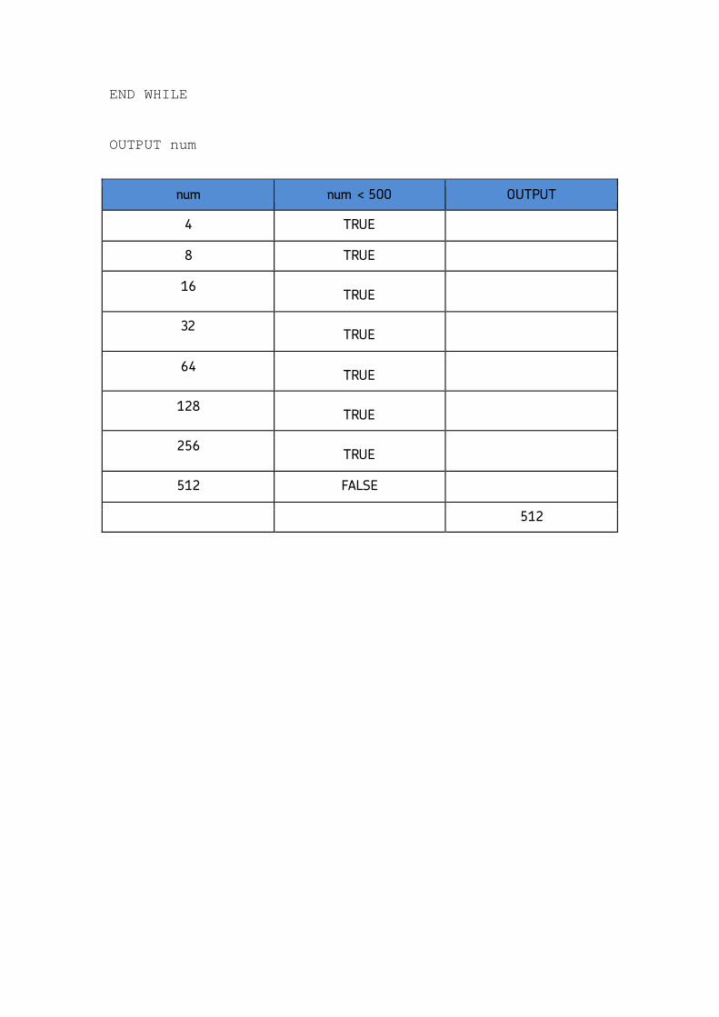
END WHILE
OUTPUT num
num num < 500 OUTPUT
4 TRUE
8 TRUE
16 TRUE
32 TRUE
64 TRUE
128 TRUE
256 TRUE
512 FALSE
512
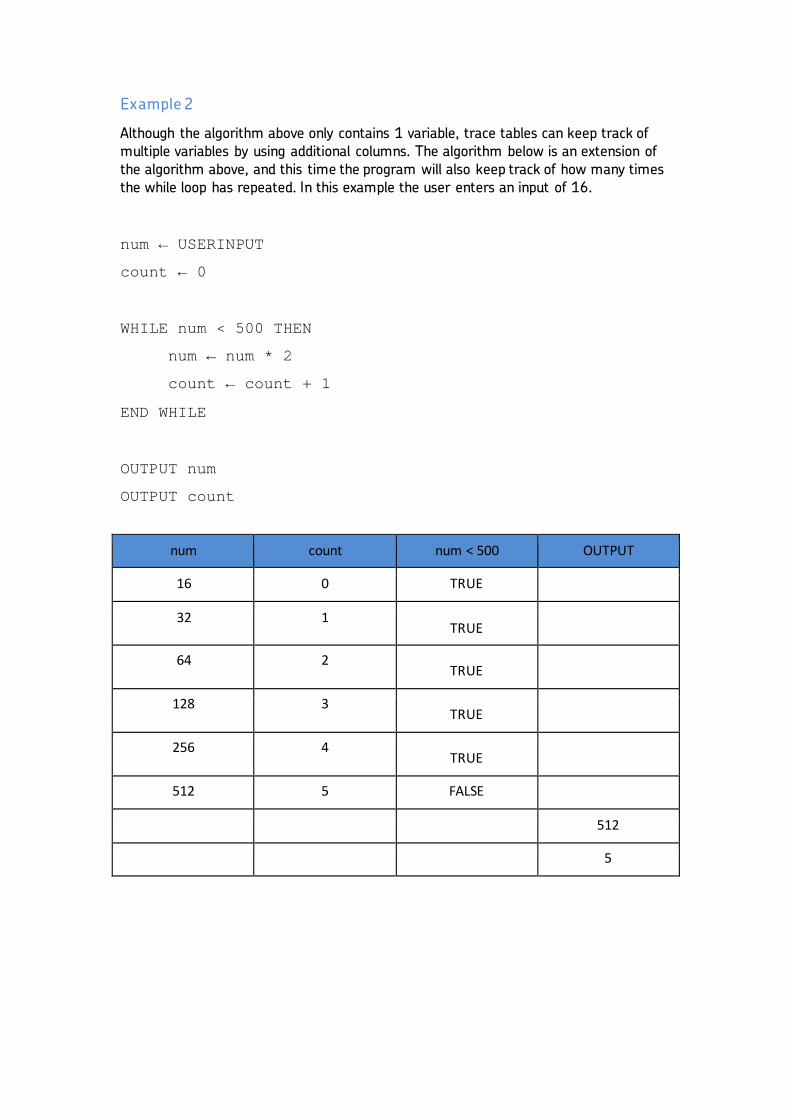
Example 2
Although the algorithm above only contains 1 variable, trace tables can keep track of multiple variables by using additional columns. The algorithm below is an extension of the algorithm above, and this time the program will also keep track of how many times the while loop has repeated. In this example the user enters an input of 16.
num ← USERINPUT
count ← 0
WHILE num < 500 THEN
num ← num * 2
count ← count + 1
END WHILE
OUTPUT num
OUTPUT count
num count num < 500 OUTPUT
16 0 TRUE
32 1 TRUE
64 2 TRUE
128 3 TRUE
256 4 TRUE
512 5 FALSE
512
5

Example 3
Trace tables help you to determine how an algorithm will run and are especially useful when you have nested structures that require you to keep track of multiple variables. The algorithm below contains a simple for loop.
FOR i ← 1 TO 4
OUTPUT i*2
ENDFOR
The trace table for this example is shown below. Although no variable is re-assigned inside the for loop, there is an output which we can keep track of with a trace table.
i Output
1 2
2 4
3 6
4 8
The algorithm below has introduced a number of additional elements which have an impact on how the algorithm runs. The best way to test this algorithm is to do a dry-run using a trace table. The trace table, with a brief explanation is shown below.
num ← 0
total ← 0
FOR i ← 1 TO 3
FOR j ← 1 TO 3
num ← j * i
total ← total + num
ENDFOR
ENDFOR
OUTPUT total
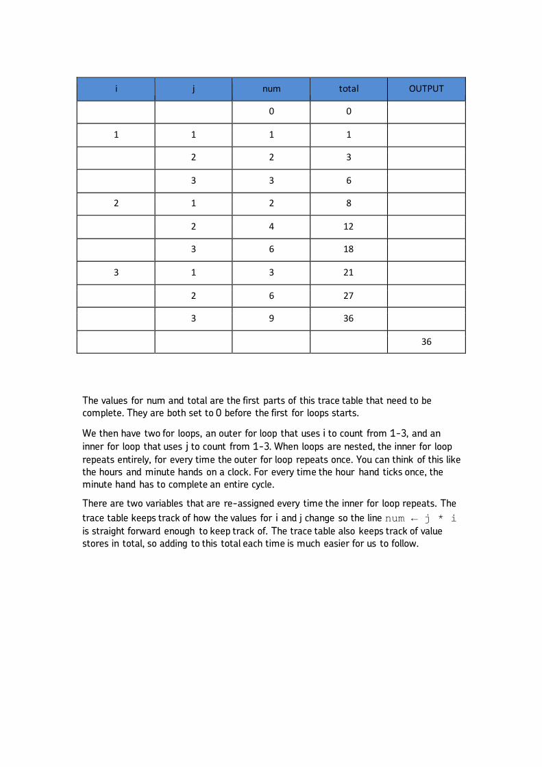
The values for num and total are the first parts of this trace table that need to be complete. They are both set to 0 before the first for loops starts.
We then have two for loops, an outer for loop that uses i to count from 1-3, and an inner for loop that uses j to count from 1-3. When loops are nested, the inner for loop repeats entirely, for every time the outer for loop repeats once. You can think of this like the hours and minute hands on a clock. For every time the hour hand ticks once, the minute hand has to complete an entire cycle.
There are two variables that are re-assigned every time the inner for loop repeats. The trace table keeps track of how the values for i and j change so the line num ← j * i is straight forward enough to keep track of. The trace table also keeps track of value stores in total, so adding to this total each time is much easier for us to follow.
i j num total OUTPUT
0 0
1 1 1 1
2 2 3
3 3 6
2 1 2 8
2 4 12
3 6 18
3 1 3 21
2 6 27
3 9 36
36

Step by step Trace Table for a Linear Search The following breaks down the process of completing a trace table for a linear search. This document is not designed to offer a full and complete explanation of how a linear search works, but focuses on the steps that are required to take a specific algorithm and complete a trace table to prove the algorithm works correctly. A linear search is an algorithm that is used to check if a specific item is present in a data structure. The algorithm loops over the data structure, comparing each item one at a time to the item that is being searched for. If the item is found the algorithm stops, but if every item in the structure is checked and no match is found, then the program will alert the user that the item is not in the structure. The pseudocode for this algorithm is shown below and the line numbers have been included so they can be referred to at different stages of the explanation in the following pages. It is advised that you continue to refer back to this page to identify specific parts of the algorithm as the trace table is gradually completed. Note: There are different ways of implementing a linear search, and while this is an accurate way of doing so, it is not the only way.
1 arrayToSearch ← [4, 8, 15, 16, 23, 42]
2
3 found ← False
4 itemToFind ← USERINPUT
5
6 FOR i ← 0 to LEN(arrayToSearch)
7 IF arrayToSearch[i] == itemToFind THEN
8 OUTPUT “Item found at index” + i
9 found ← True
10 BREAK
11 i ← i + 1
12 END FOR
13
14 IF found == False THEN
15 OUTPUT “The item is not in the list”
16 END IF
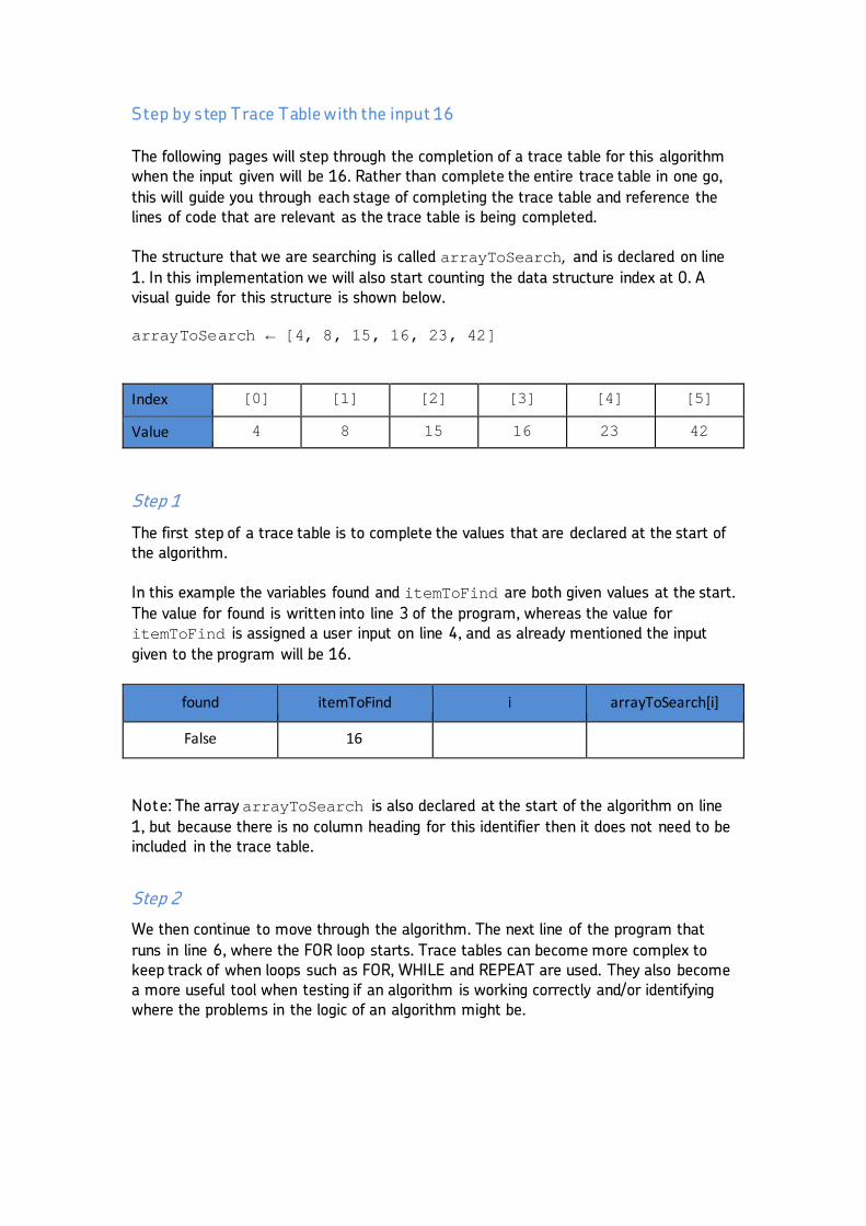
Step by step Trace Table with the input 16 The following pages will step through the completion of a trace table for this algorithm when the input given will be 16. Rather than complete the entire trace table in one go, this will guide you through each stage of completing the trace table and reference the lines of code that are relevant as the trace table is being completed. The structure that we are searching is called arrayToSearch, and is declared on line 1. In this implementation we will also start counting the data structure index at 0. A visual guide for this structure is shown below. arrayToSearch ← [4, 8, 15, 16, 23, 42]
Index [0] [1] [2] [3] [4] [5]
Value 4 8 15 16 23 42
Step 1
The first step of a trace table is to complete the values that are declared at the start of the algorithm. In this example the variables found and itemToFind are both given values at the start. The value for found is written into line 3 of the program, whereas the value for itemToFind is assigned a user input on line 4, and as already mentioned the input given to the program will be 16.
found itemToFind i arrayToSearch[i]
False 16
Note: The array arrayToSearch is also declared at the start of the algorithm on line 1, but because there is no column heading for this identifier then it does not need to be included in the trace table.
Step 2
We then continue to move through the algorithm. The next line of the program that runs in line 6, where the FOR loop starts. Trace tables can become more complex to keep track of when loops such as FOR, WHILE and REPEAT are used. They also become a more useful tool when testing if an algorithm is working correctly and/or identifying where the problems in the logic of an algorithm might be.
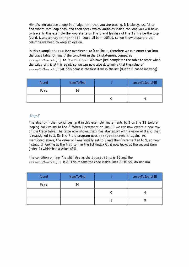
Hint: When you see a loop in an algorithm that you are tracing, it is always useful to find where that loop ends, and then check which variables inside the loop you will have to trace. In this example the loop starts on line 6 and finishes of line 12. Inside the loop found, i, and arrayToSearch[i] could all be modified, so we know those are the columns we need to keep an eye on. In this example the FOR loop initialises i to 0 on line 6, therefore we can enter that into the trace table. On line 7 the condition in the IF statement compares arrayToSearch[i] to itemToFind. We have just completed the table to state what the value of i is at this point, so we can now also determine that the value of arrayToSearch[i]at this point is the first item in the list (due to 0 based indexing).
found itemToFind i arrayToSearch[i]
False 16
0 4
Step 3
The algorithm then continues, and in this example i increments by 1 on line 11, before looping back round to line 6. When i increment on line 11 we can now create a new row on the trace table. The table now shows that i has started off with a value of 0 and then is reassigned to 1. On line 7 the program uses arrayToSearch[i]again. As mentioned above, the value of i was initially set to 0 and then incremented to 1, so now instead of looking at the first item in the list (index 0), it now looks at the second item (index 1) which has a value of 8. The condition on line 7 is still false as the itemToFind is 16 and the arrayToSearch[i] is 8. This means the code inside lines 8-10 still do not run.
found itemToFind i arrayToSearch[i]
False 16
0 4
1 8

Step 4
The next step in this example is very similar to Step 3. Line 11 increments the value of I by 1 again, which means it now has a value of 2. The loop repeats back round to line 6 and then the condition on line 7 is checked again. With the value of i now being 2, the arrayToSearch[i] is now the third item in the list, which is a value of 15. Again, this condition is false so lines 8-10 are skipped.
found itemToFind i arrayToSearch[i]
False 16
0 4
1 8
2 15
Step 5
With lines 8-10 being skipped, the program then moves onto line 11, where i increments by 1 so it has a value of 3. Just like in step 2, step 3 and step 4, i is used to look at the next item in the list, so this time around arrayToSearch[i] has a value of 16. The condition on line 7 is now comparing arrayToSearch[i] and itemToFind both of which have a value of 16. This condition is therefore TRUE and so for the first time in this program lines 8-10 are run. In the HINT for Step 2 it was mentioned that it is good practice to keep track of any variables that have the potential to be re-assigned in a loop. This loop is now in its 4th iteration, and for the first time lines 8-10 have been run. Line 8 is an output which is not asked for in the trace table, but line 9 re-assigns the value for found, so we can change the value of found in the trace table to TRUE. Line 10 then runs for the first time in this program, and this breaks the FOR loops and takes us down to line 12 for the rest of the program to be completed. At this point we can see that none of the remaining lines of code will change any of the variables or values required in our trace table, so this is now complete.
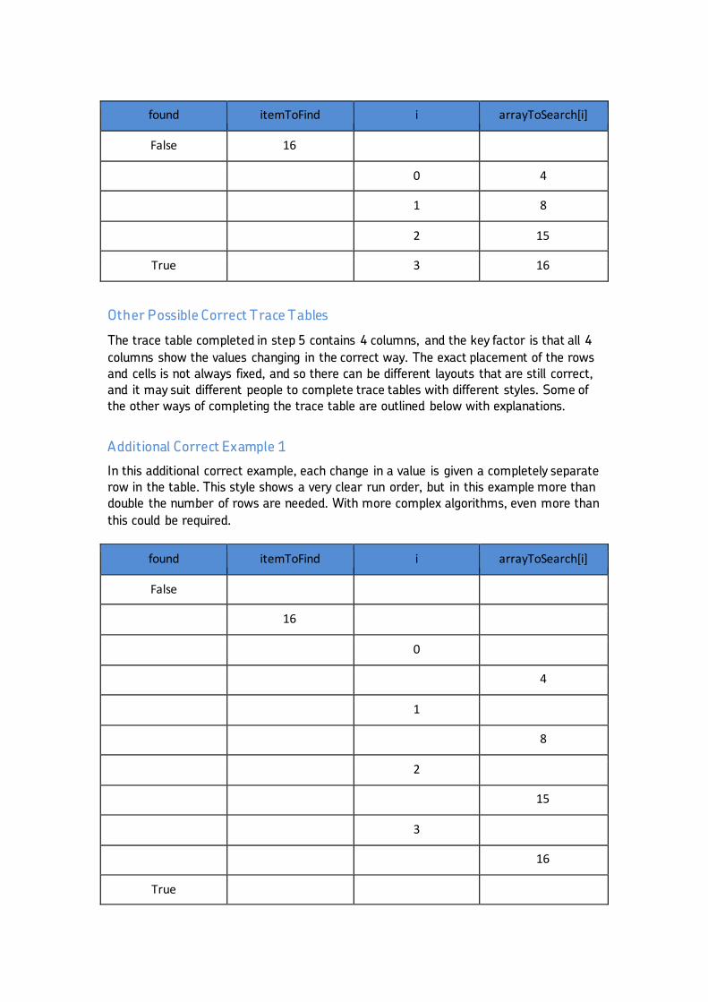
found itemToFind i arrayToSearch[i]
False 16
0 4
1 8
2 15
True 3 16
Other Possible Correct Trace Tables
The trace table completed in step 5 contains 4 columns, and the key factor is that all 4 columns show the values changing in the correct way. The exact placement of the rows and cells is not always fixed, and so there can be different layouts that are still correct, and it may suit different people to complete trace tables with different styles. Some of the other ways of completing the trace table are outlined below with explanations.
Additional Correct Example 1
In this additional correct example, each change in a value is given a completely separate row in the table. This style shows a very clear run order, but in this example more than double the number of rows are needed. With more complex algorithms, even more than this could be required.
found itemToFind i arrayToSearch[i]
False
16
0
4
1
8
2
15
3
16
True

Additional Correct Example 2
The original trace table completed in step 5 shows when the values for each column change. In this additional correct example, every cell is complete, even if the value does not change. The advantage of this method is that making comparisons is clearer, but the disadvantage is that if the algorithm hasn’t been understood properly and changes need to be made, the trace table can begin to look very messy and difficult to read.
found itemToFind i arrayToSearch[i]
False 16
False 16 0 4
False 16 1 8
False 16 2 15
True 16 3 16
The key point to both of these additional correct examples is that the values in each column change in the correct way. • The column for found starts off as False as identified in line 3, and then is changed
to True at the end when line 9 will run. • itemToFind starts off as 16 and does not change throughout the trace table. • i starts as 0 and continues to count to 3 in increments of 1, but does not go beyond 3. • arrayToSearch[i] starts off as 4 and then continues to show value for each
item one at a time until it gets to 16, but again, does not go any further.
Common Mistakes
There are some common mistakes that can occur when completing trace tables, even if the person completing the table has fully understood the algorithm. Two of these common mistakes are outlined below, and both provide examples based on an input of 16.
Auto-Completing rows and values without considering when the values should stop changing
In this example the person completing the trace table has identified that the loop could potentially count from 0-5, and that this will be used to cycle through each item in the list. Rather than tracing the values one at a time, they have assumed the program will continue and have completed the table without considering when the break may actually occur.
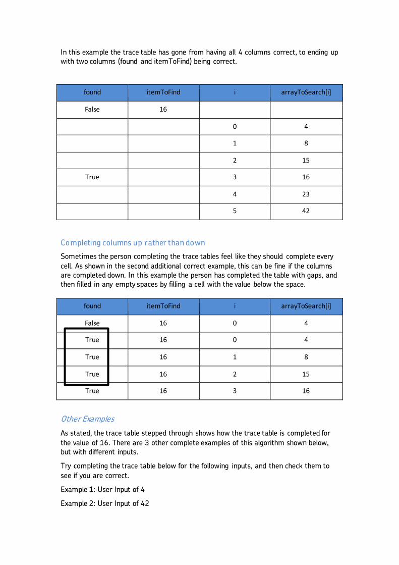
In this example the trace table has gone from having all 4 columns correct, to ending up with two columns (found and itemToFind) being correct.
found itemToFind i arrayToSearch[i]
False 16
0 4
1 8
2 15
True 3 16
4 23
5 42
Completing columns up rather than down
Sometimes the person completing the trace tables feel like they should complete every cell. As shown in the second additional correct example, this can be fine if the columns are completed down. In this example the person has completed the table with gaps, and then filled in any empty spaces by filling a cell with the value below the space.
found itemToFind i arrayToSearch[i]
False 16 0 4
True 16 0 4
True 16 1 8
True 16 2 15
True 16 3 16
Other Examples
As stated, the trace table stepped through shows how the trace table is completed for the value of 16. There are 3 other complete examples of this algorithm shown below, but with different inputs.
Try completing the trace table below for the following inputs, and then check them to see if you are correct.
Example 1: User Input of 4
Example 2: User Input of 42
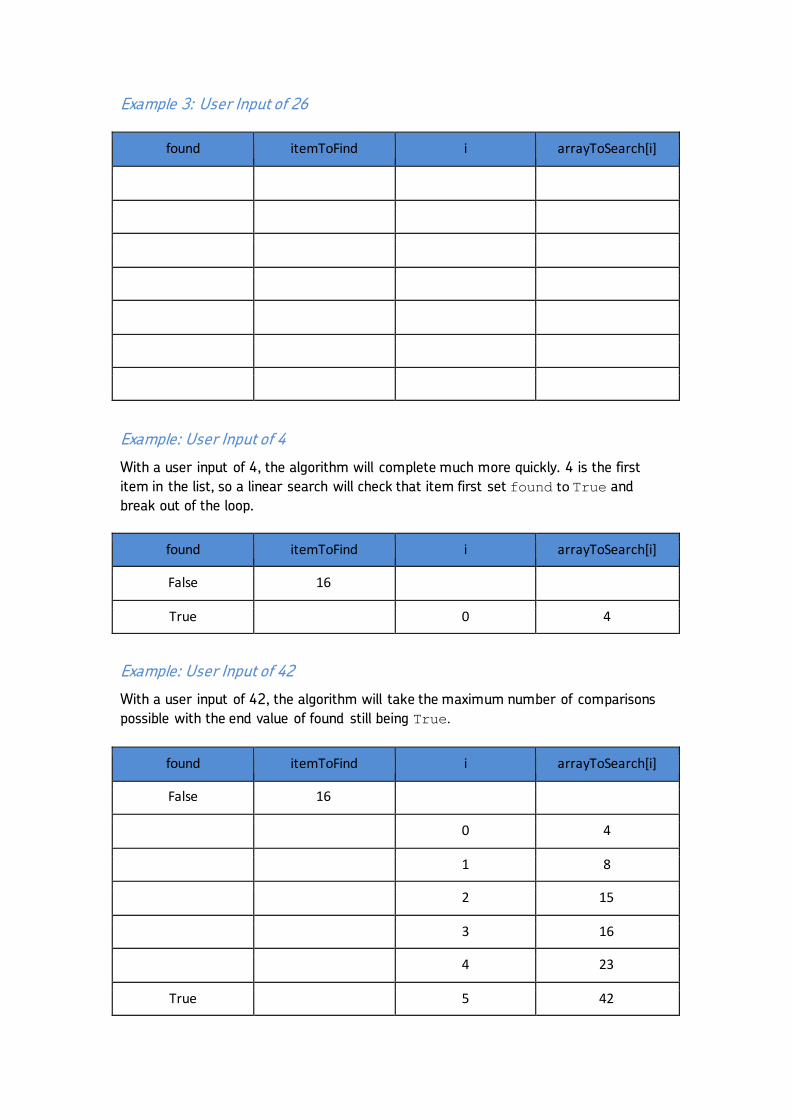
Example 3: User Input of 26
found itemToFind i arrayToSearch[i]
Example: User Input of 4
With a user input of 4, the algorithm will complete much more quickly. 4 is the first item in the list, so a linear search will check that item first set found to True and break out of the loop.
found itemToFind i arrayToSearch[i]
False 16
True 0 4
Example: User Input of 42
With a user input of 42, the algorithm will take the maximum number of comparisons possible with the end value of found still being True.
found itemToFind i arrayToSearch[i]
False 16
0 4
1 8
2 15
3 16
4 23
True 5 42

Example: User Input of 26
With a user input of 26, the algorithm will cycle through every item in the list, but because it will be unable to find it, the end value of found will remain as false.
found itemToFind i arrayToSearch[i]
False 16
0 4
1 8
2 15
3 16
4 23
False 5 42
Teaching Strategies to Introduce Trace Tables
One reason that trace tables often seem very challenging to students is that they are not introduced at an early stage of programming. Students will go through the basic skills required and won’t see trace tables until they are faced with more complex algorithms. There are many ways the concepts to build the skills to complete trace tables can be introduced earlier in a student’s programming development. This section looks at some of these using the Micro:bit block language, and Python. Note: While the following examples use the Micro:bit block language or Python, these activities could be created in other block languages such as Scratch, or programming languages such as Small Basic or VB. The key idea is finding ways to introduce the concepts of variable tracing in whatever language students are first introduced to programming with.
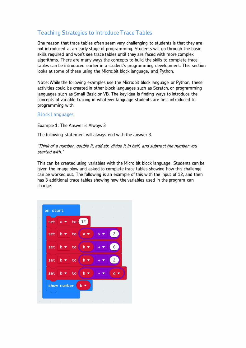
Block Languages Example 1: The Answer is Always 3
The following statement will always end with the answer 3. ‘Think of a number, double it, add six, divide it in half, and subtract the number you started with.’ This can be created using variables with the Micro:bit block language. Students can be given the image blow and asked to complete trace tables showing how this challenge can be worked out. The following is an example of this with the input of 12, and then has 3 additional trace tables showing how the variables used in the program can change.

Input: 12 Input: 4 Input: 0 Input: 3
A B A B A B A B
12 4 0 3
24 8 0 6
30 14 6 12
15 7 3 6
3 3 3 3
Other Micro:bit Trace Tables
While the programs below may not be useful in solving specific problems, they can be an effective way of showing how trace tables can be completed at an early stage of a student’s programming development. This method also has the added benefit of allowing the student to complete the trace table based on the program, and then test the program with either the online emulator or a Micro:bit to see if they have the correct end value. Example 1

A B
10
12
27
54
18
972
947
Example 2 The following example has added additional programming concepts in the form of IF statement as well as conditions that have their own column in the trace tables.
Trace table for the above algorithm with the inputs a = 6, b = 4 and c = 12

A B C A < B
6 4 12 False
2
24
26
Trace table for the above algorithm with the inputs a = 50, b = 60 and c = 70
A B C A < B
50 60 70 True
110
-40
-4,400
Example 3 This final example adds a further programming concept in the form of a repeat loop. An index is used to count inside the loop and an OUPUT is added to the trace table.
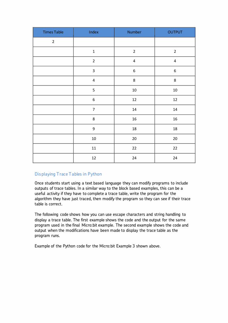
Times Table Index Number OUTPUT
2
1 2 2
2 4 4
3 6 6
4 8 8
5 10 10
6 12 12
7 14 14
8 16 16
9 18 18
10 20 20
11 22 22
12 24 24
Displaying Trace Tables in Python
Once students start using a text based language they can modify programs to include outputs of trace tables. In a similar way to the block based examples, this can be a useful activity if they have to complete a trace table, write the program for the algorithm they have just traced, then modify the program so they can see if their trace table is correct. The following code shows how you can use escape characters and string handling to display a trace table. The first example shows the code and the output for the same program used in the final Micro:bit example. The second example shows the code and output when the modifications have been made to display the trace table as the program runs. Example of the Python code for the Micro:bit Example 3 shown above.
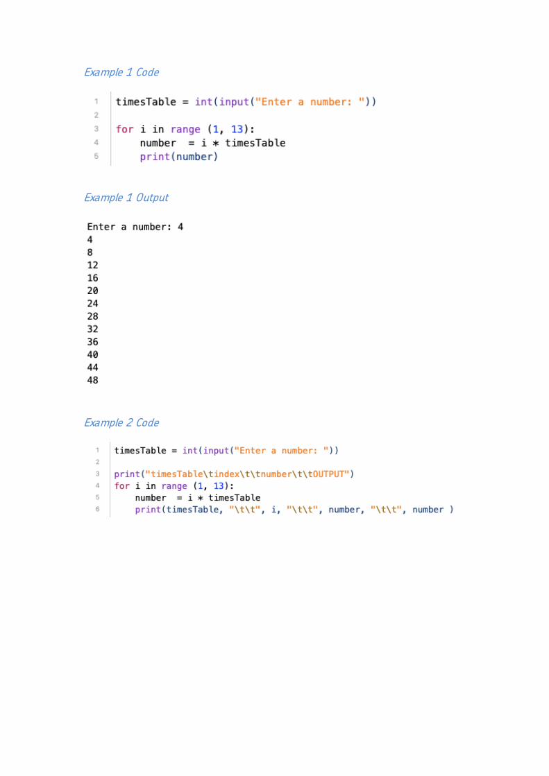
Example 1 Code
Example 1 Output
Example 2 Code

Example 2 Output
The main syntax used to create this is a TAB space that’s added to a string by using “\t” inside a string. The column headings are displayed with the TAB space before the loop starts. Inside, the loop all of the variables being traced are concatenated with the TAB spaces to line up with the headings.