technical assistance document for sampling and analysis of ... · some types of instruments...
TRANSCRIPT

TECHNICAL ASSISTANCE DOCUMENT FOR SAMPLING AND ANALYSIS OF OZONE PRECURSORS FOR THE PHOTOCHEMICAL ASSESSMENT MONITORING STATIONS PROGRAM - Revision 2 - April 2019

ii
EPA-454/B-19-004 April 2019
TECHNICAL ASSISTANCE DOCUMENT FOR SAMPLING AND ANALYSIS OF OZONE PRECURSORS FOR THE PHOTOCHEMICAL ASSESSMENT MONITORING STATIONS
PROGRAM - Revision 2 - April 2019
U.S. Environmental Protection Agency Office of Air Quality Planning and Standards
Air Quality Assessment Division Research Triangle Park, NC

PAMS Required Site Network TAD EPA-454/B-19-004 April 2019
iii
DISCLAIMER
The statements in this document, with the exception of referenced requirements, are intended solely as guidance. This document is not intended, nor can it be relied upon, to create any rights enforceable by any party in litigation with the United States. The Environmental Protection Agency (EPA) may decide to follow the guidance provided in this document, or to act at variance with the guidance based on its analysis of the specific facts presented. Mention of commercial products or trade names should not be interpreted as endorsement. Some types of instruments currently in use may be described in text or in example figures or tables. Sometimes these products are given as a typical and perhaps well-known example of the general class of instruments. Other instruments in the class are available and may be fully acceptable.

PAMS Required Site Network TAD EPA-454/B-19-004 April 2019
iv
CONTENTS 1.0 INTRODUCTION ................................................................................................................. 1
1.1 Scope and Purpose ........................................................................................................ 1 1.2 Overview of TAD Sections ........................................................................................... 2
1.2.1 Notable Changes from the 1998 TAD .............................................................. 2 1.3 Background ................................................................................................................... 3 1.4 References ..................................................................................................................... 4
2.0 UPDATED REGULATIONS ................................................................................................ 5
2.1 PAMS Required Sites – Collocation with NCore ......................................................... 5 2.2 PAMS Parameters ......................................................................................................... 6 2.3 References ..................................................................................................................... 9
3.0 DATA QUALITY PLANNING AND QUALITY ASSURANCE ..................................... 10
3.1 Data Quality Objectives .............................................................................................. 10 3.2 Data Quality Indicators ............................................................................................... 10 3.3 Measurement Quality Objectives ................................................................................ 11
3.3.1 Representativeness .......................................................................................... 12 3.3.1.1 Temporal Representativeness ............................................................. 12 3.3.1.2 Spatial Representativeness – Chemical Measurement Probe
Siting Criteria ...................................................................................... 13 3.3.1.2.1 Inlet Probe Height ............................................................. 13 3.3.1.2.2 Spacing from Obstructions ............................................... 14 3.3.1.2.3 Spacing from Trees ........................................................... 14 3.3.1.2.4 Spacing from Roadways ................................................... 14
3.3.1.3 Spatial Representativeness – Meteorological Parameters ................... 14 3.3.2 Completeness .................................................................................................. 16
3.3.2.1 Make-up Sample Policy – Carbonyls Only ........................................ 17 3.3.3 Precision .......................................................................................................... 18 3.3.4 Bias ................................................................................................................. 20
3.3.4.1 Assessing Laboratory Bias .................................................................. 21 3.3.4.2 Assessing Field Measurement Bias .................................................... 21
3.3.4.2.1 Field Site Proficiency Testing for Speciated VOCs ......... 21 3.3.4.2.2 Assessing Field Bias for Carbonyls .................................. 22 3.3.4.2.3 Ongoing Bias Assessment for Speciated VOCs and
Continuous Gas Monitors ................................................. 22 3.3.4.2.4 Through-the-Probe Auditing ............................................. 23
3.3.5 Sensitivity ....................................................................................................... 23 3.3.5.1 Method Detection Limits .................................................................... 24
3.3.5.1.1 Frequency of Method Detection Limit Determination ................................................................... 28
3.3.5.1.2 MDL Measurement Quality Objectives ............................ 29 3.3.5.1.3 Determining MDLs via 40 CFR Part 136 Appendix
B – Method Update Rule .................................................. 29 3.4 Quality Assurance Project Plan .................................................................................. 34

PAMS Required Site Network TAD EPA-454/B-19-004 April 2019
v
3.4.1 Development of the National PAMS Required Site Program QAPP ............. 35 3.4.2 PAMS Required Site QAPP Program Deviations .......................................... 36
3.5 Standard Operating Procedures ................................................................................... 36 3.6 Good Scientific Practices ............................................................................................ 38
3.6.1 Data Consistency and Traceability ................................................................. 38 3.7 References ................................................................................................................... 38
4.0 VOLATILE ORGANIC COMPOUNDS BY AUTO-GC ................................................... 40
4.1 Priority and Optional Volatile Organic Compounds .................................................. 40 4.2 Instrumentation – Measuring VOCs with an Auto Gas Chromatograph with
Flame Ionization Detection ...................................................................................... 42 4.2.1 Summary of Method ....................................................................................... 42 4.2.2 Sample Introduction and Collection ............................................................... 43
4.2.2.1 Probe Inlet ........................................................................................... 43 4.2.2.2 Sample Collection Requirements ........................................................ 45
4.2.3 Automatic Gas Chromatograph (Auto-GC) .................................................... 45 4.2.3.1 Instrument Sensitivity ......................................................................... 46 4.2.3.2 Moisture Management ........................................................................ 46 4.2.3.3 Thermal Desorption ............................................................................ 48 4.2.3.4 Separation of Compounds ................................................................... 50 4.2.3.5 Flame Ionization Detection ................................................................. 50
4.2.4 Compound Identification ................................................................................ 51 4.2.4.1 Compound Retention Time ................................................................. 51 4.2.4.2 Signal-to-Noise Ratio .......................................................................... 53
4.2.5 Auto-GC Data File Naming ............................................................................ 54 4.3 Method Detection Limits for Auto-GC ....................................................................... 55
4.3.1 MDL Blank Component, MDLb ..................................................................... 56 4.3.2 MDL Standard Spike Component, MDLsp ..................................................... 56 4.3.3 Redetermination of MDLs .............................................................................. 59
4.4 Auto-GC Interferences ................................................................................................ 59 4.4.1 Ozone Interference .......................................................................................... 59 4.4.2 Moisture .......................................................................................................... 60 4.4.3 Temperature .................................................................................................... 60 4.4.4 Source-Oriented Interferences ........................................................................ 61 4.4.5 Problematic Compounds for Auto-GC ........................................................... 62
4.5 Calibration of Auto-GCs ............................................................................................. 63 4.5.1 Standard Materials .......................................................................................... 63
4.5.1.1 Primary Calibration Standard ............................................................. 63 4.5.1.2 Secondary Source Calibration Verification Standard ......................... 63 4.5.1.3 Retention Time Standard .................................................................... 64 4.5.1.4 Zero Air ............................................................................................... 64
4.5.2 Retention Time Establishment and Calibration Convention and Procedure ........................................................................................................ 65
4.5.2.1 Static Dilution ..................................................................................... 66 4.5.2.2 Dynamic Dilution................................................................................ 68 4.5.2.3 Pulsed Standard Delivery .................................................................... 70

PAMS Required Site Network TAD EPA-454/B-19-004 April 2019
vi
4.5.2.4 Humidification .................................................................................... 71 4.5.3 Auto-GC Calibration Curves .......................................................................... 72 4.5.4 Second Source Calibration Verification ......................................................... 73
4.6 Auto-GC Operation and Quality Control .................................................................... 73 4.6.1 System Blanks ................................................................................................. 76 4.6.2 Continuing Calibration Verification (CCV) ................................................... 77 4.6.3 Precision Check .............................................................................................. 77 4.6.4 Retention Time Standard ................................................................................ 77
4.7 References ................................................................................................................... 80 5.0 CARBONYL COMPOUNDS VIA EPA COMPENDIUM METHOD TO-11A ................ 83
5.1 General Description of Sampling Method and Analytical Method ............................ 83 5.2 Minimizing Bias.......................................................................................................... 84 5.3 Carbonyls Precision .................................................................................................... 84
5.3.1 Sampling Precision ......................................................................................... 85 5.3.1.1 Collocated Sample Collection ............................................................. 85 5.3.1.2 Duplicate Sample Collection .............................................................. 86
5.3.2 Laboratory Precision ....................................................................................... 87 5.4 Managing Ozone ......................................................................................................... 87
5.4.1 Copper Tubing Denuder/Scrubber .................................................................. 88 5.4.2 Sorbent Cartridge Scrubbers ........................................................................... 89 5.4.3 Other Ozone Scrubbers ................................................................................... 89
5.5 Collection Media ......................................................................................................... 89 5.5.1 Lot Evaluation and Acceptance Criteria ......................................................... 89 5.5.2 Cartridge Handling and Storage...................................................................... 90 5.5.3 Damaged Cartridges........................................................................................ 91 5.5.4 Cartridge Shelf Life ........................................................................................ 91
5.6 Carbonyls Method Detection Limits ........................................................................... 91 5.6.1 Carbonyls MDL Procedure ............................................................................. 92
5.6.1.1 Selecting a Spiking Level ................................................................... 92 5.6.1.2 Preparing MDL Spikes and Blanks..................................................... 93 5.6.1.3 Extraction and Analysis of MDL Spikes and Blanks ......................... 93 5.6.1.4 MDL Calculation ................................................................................ 93 5.6.1.5 Ongoing Determination of MDLs ....................................................... 95
5.6.2 Example Carbonyls MDL Scenario and Calculation ...................................... 96 5.7 Carbonyls Sample Collection Equipment, Certification, and Maintenance ............... 97
5.7.1 Sampling Equipment ....................................................................................... 98 5.7.1.1 Sampling Unit Zero Check (Positive Bias Check) ............................. 98 5.7.1.2 Carbonyls Sampling Unit Flow Calibration ....................................... 99 5.7.1.3 Moisture Management ...................................................................... 100
5.7.2 Sampling Train Configuration and Presample Purge ................................... 100 5.7.3 Carbonyl Sampling Inlet Maintenance ......................................................... 101
5.8 Sample Collection Procedures and Field Quality Control Samples ......................... 101 5.8.1 Sample Collection Procedures ...................................................................... 101
5.8.1.1 Sample Setup .................................................................................... 101 5.8.1.2 Sample Retrieval ............................................................................... 102

PAMS Required Site Network TAD EPA-454/B-19-004 April 2019
vii
5.8.1.3 Sampling Schedule and Duration...................................................... 103 5.8.1.4 Carbonyls Sample Chain of Custody ................................................ 103
5.8.2 Field Quality Control Samples...................................................................... 104 5.8.2.1 Field Blanks and Exposure Blanks ................................................... 104 5.8.2.2 Trip Blanks........................................................................................ 105 5.8.2.3 Collocated Samples ........................................................................... 106 5.8.2.4 Duplicate Samples ............................................................................ 106 5.8.2.5 Field Matrix Spikes ........................................................................... 106 5.8.2.6 Breakthrough Samples ...................................................................... 107
5.9 Carbonyls Extraction and Analysis ........................................................................... 107 5.9.1 Analytical Interferences and Contamination ................................................ 107
5.9.1.1 Analytical Interferences .................................................................... 107 5.9.1.2 Labware Cleaning ............................................................................. 107 5.9.1.3 Minimizing Sources of Contamination ............................................. 108
5.9.2 Reagents and Standard Materials .................................................................. 108 5.9.2.1 Solvents ............................................................................................. 108 5.9.2.2 Calibration Stock Materials .............................................................. 108 5.9.2.3 Secondary Source Calibration Verification Stock Materials ............ 109 5.9.2.4 Holding Time and Storage Requirements ......................................... 109
5.9.3 Cartridge Holding Time and Storage Requirements ..................................... 109 5.9.4 Cartridge Extraction ...................................................................................... 109
5.9.4.1 Laboratory Extraction Batch Quality Control Samples .................... 109 5.9.4.2 Cartridge Extraction Procedures ....................................................... 110
5.9.5 Analysis by HPLC ........................................................................................ 111 5.9.5.1 Instrumentation Specifications.......................................................... 111 5.9.5.2 Initial Calibration .............................................................................. 111 5.9.5.3 Secondary Source Calibration Verification Standard ....................... 112 5.9.5.4 Continuing Calibration Verification ................................................. 112 5.9.5.5 Replicate Analysis ............................................................................ 113 5.9.5.6 Compound Identification .................................................................. 113 5.9.5.7 Data Review and Concentration Calculations .................................. 114
5.10 Summary of Quality Control Parameters .................................................................. 116 5.11 References ................................................................................................................. 119
6.0 OXIDES OF NITROGEN ................................................................................................. 120
6.1 NO/NOy..................................................................................................................... 121 6.2 True NO2 ................................................................................................................... 121
6.2.1 Photolytic Conversion Chemiluminescent Detection NO2 Instruments ....... 121 6.2.2 Cavity Attenuated Phase Shift (CAPS) Instruments ..................................... 123 6.2.3 Cavity Ring-down Spectroscopy (CRDS) Instruments ................................ 124 6.2.4 True NO2 FEM Instrument Response ........................................................... 124 6.2.5 Minimizing Bias in NO2 Measurements ....................................................... 125 6.2.6 Generation of NO2 Standards ........................................................................ 126
6.2.6.1 Gas Phase Titration ........................................................................... 126 6.2.6.2 Dilution of Standard NO2 Gas .......................................................... 127
6.2.7 Calibration of True NO2 Instruments ............................................................ 128

PAMS Required Site Network TAD EPA-454/B-19-004 April 2019
viii
6.2.8 True NO2 Sampling ....................................................................................... 128 6.2.9 Method Detection Limits for Continuous Gaseous Criteria Pollutant
Methods......................................................................................................... 128 6.2.9.1 Determining the MDLb ..................................................................... 129 6.2.9.2 Determining the MDLsp .................................................................... 130 6.2.9.3 Calculating and Verifying the Instrument MDL ............................... 131 6.2.9.4 Ongoing Determination of the Instrument MDL .............................. 132 6.2.9.5 Example MDL Calculation for Continuous Gaseous Criteria
Pollutant Monitors ............................................................................ 132 6.2.10 True NO2 Quality Control ............................................................................. 134
6.3 NOy ........................................................................................................................... 135 6.4 References ................................................................................................................. 136
7.0 OZONE .............................................................................................................................. 138
7.1 References ................................................................................................................. 139 8.0 METEOROLOGY ............................................................................................................. 140
8.1 Wind Speed and Wind Direction .............................................................................. 140 8.2 Temperature .............................................................................................................. 141 8.3 Relative Humidity ..................................................................................................... 142 8.4 Solar Radiation.......................................................................................................... 143 8.5 Ultraviolet Radiation ................................................................................................. 143 8.6 Barometric Pressure .................................................................................................. 144 8.7 Precipitation .............................................................................................................. 144 8.8 Mixing Layer Height................................................................................................. 144
8.8.1 Definition and Measurement of Mixing Layer Height ................................. 144 8.8.2 Ceilometer Theory of Operation ................................................................... 146 8.8.3 Ceilometer Siting and Installation ................................................................ 148 8.8.4 Ceilometer Operations .................................................................................. 149 8.8.5 Ceilometer Mixing Height Calculations ....................................................... 149 8.8.6 Mixing Height Data Files and Data Validation ............................................ 151
8.9 Quality Assurance/Quality Control for Meteorological Measurements ................... 152 8.10 References ................................................................................................................. 155
9.0 DATA HANDLING .......................................................................................................... 156
9.1 Data Collection ......................................................................................................... 156 9.1.1 Validation of Data Reduction and Transformation Systems and
Software ........................................................................................................ 156 9.2 Data Backup .............................................................................................................. 156 9.3 Recording of Data ..................................................................................................... 157
9.3.1 Paper Records ............................................................................................... 157 9.3.2 Electronic Data Capture ................................................................................ 157 9.3.3 Error Correction ............................................................................................ 157
9.3.3.1 Manual Integration of Chromatographic Peaks ................................ 158 9.4 Numerical Calculations ............................................................................................. 158
9.4.1 Rounding ....................................................................................................... 159

PAMS Required Site Network TAD EPA-454/B-19-004 April 2019
ix
9.4.2 Calculations Using Significant Digits ........................................................... 159 9.4.2.1 Addition and Subtraction .................................................................. 159 9.4.2.2 Multiplication and Division .............................................................. 159 9.4.2.3 Standard Deviation ............................................................................ 160 9.4.2.4 Logarithms ........................................................................................ 160
9.5 In-house Control Limits ............................................................................................ 160 9.5.1 Warning Limits ............................................................................................. 160 9.5.2 Control Limits ............................................................................................... 161
9.6 Negative Values ........................................................................................................ 161 9.6.1 Negative Concentrations ............................................................................... 161 9.6.2 Negative Physical Measurements ................................................................. 161
10.0 PAMS DATA VERIFICATION AND VALIDATION .................................................... 162
10.1 Data Verification ....................................................................................................... 164 10.1.1 Routine (Self) Review ................................................................................... 165 10.1.2 Technical Review.......................................................................................... 167
10.2 Data Validation ......................................................................................................... 168 10.2.1 Level 1 Data Validation ................................................................................ 169
10.2.1.1 Identification of Outliers ................................................................... 170 10.2.2 Level 2 Data Validation ................................................................................ 171 10.2.3 Level 3 Data Validation ................................................................................ 171
10.3 Reporting of Validated Data to AQS ........................................................................ 171 10.3.1 Reporting Values below Method Detection Limits ...................................... 171
10.4 Data Validation Tools and Methods ......................................................................... 172 10.4.1 Data Validation Visualization Methods ........................................................ 172 10.4.2 Data Validation Tools ................................................................................... 178
10.5 Data Verification and Validation Records ................................................................ 179 10.6 Data Flagging ............................................................................................................ 179 10.7 Data Verification and Validation of Speciated VOCs .............................................. 179
10.7.1 Speciated VOCs Data Sources ...................................................................... 180 10.7.1.1 Calibration Data ................................................................................ 180 10.7.1.2 Auto-GC Reports and Datafiles ........................................................ 180 10.7.1.3 Chromatographic Data File Identification ........................................ 181 10.7.1.4 Auto-GC Chromatograms ................................................................. 181 10.7.1.5 Instrument Maintenance and Site Logbooks ..................................... 183
10.7.2 Speciated VOCs Data Verification Procedures ............................................ 183 10.7.2.1 Correcting Chromatography Data ..................................................... 184 10.7.2.2 Routine Auto-GC Operator Checks .................................................. 184 10.7.2.3 Technical Review of Speciated VOCs Data ..................................... 185
10.7.3 Speciated VOCs Data Validation Procedures ............................................... 191 10.7.3.1 Level 1 Data Validation .................................................................... 192 10.7.3.2 Level 2 Data Validation - Historical Data Comparisons .................. 193 10.7.3.3 Level 3 Data Validation - Parallel Consistency Checks ................... 193
10.7.4 Speciated VOCs Visualization Methods ....................................................... 193 10.7.4.1 Time Series Graphs ........................................................................... 193 10.7.4.2 Scatter Plots ...................................................................................... 194

PAMS Required Site Network TAD EPA-454/B-19-004 April 2019
x
10.7.4.3 Fingerprint Plots................................................................................ 194 10.7.4.4 Comparison with Other Parameters .................................................. 194
10.8 Carbonyl Data Verification and Validation .............................................................. 195 10.8.1 Site Operator Verification Activities ............................................................ 196 10.8.2 ASL Verification and Validation Activities ................................................. 196
10.8.2.1 ASL Sample Receipt ......................................................................... 196 10.8.2.2 ASL Sample Extraction .................................................................... 197 10.8.2.3 ASL Sample Analysis ....................................................................... 197 10.8.2.4 ASL Overall Technical Review ........................................................ 197
10.8.3 Carbonyls SLT Monitoring Agency Data Verification and Validation ........ 200 10.8.3.1 Manual Inspection of Carbonyls Collection Data ............................. 200 10.8.3.2 Review of ASL Data ......................................................................... 201 10.8.3.3 Review of Supporting QC Data ........................................................ 201 10.8.3.4 SLT Monitoring Agency Carbonyls Data Validation ....................... 202
10.8.3.4.1 Level 1 Carbonyls Data Validation ................................. 202 10.8.3.4.2 Level 2 Carbonyls Data Validation ................................. 204 10.8.3.4.3 Level 3 Carbonyls Data Validation ................................. 204
10.9 Data Verification and Validation of Ozone and Nitrogen Oxides ............................ 210 10.9.1 Ozone ............................................................................................................ 211 10.9.2 Nitrogen Oxides, including True NO2 .......................................................... 212
10.10 Verification and Validation of Routine Meteorological Measurements ................ 212 10.10.1 Routine Meteorology Data Verification ....................................................... 212
10.10.1.1 Site Operator Routine Checks ........................................................ 213 10.10.1.2 Data Verification Performed by DAS ............................................ 215 10.10.1.3 Technical Review of Meteorology Data ........................................ 215
10.10.2 Meteorology Data Validation ....................................................................... 216 10.10.2.1 Level 1 Validation of Meteorology Data ....................................... 216 10.10.2.2 Level 2 Validation of Meteorology Data ....................................... 217 10.10.2.3 Level 3 Validation of Meteorology Data ....................................... 217 10.10.2.4 Reporting Validated Data to AQS ................................................. 218
10.11 Using Surface Meteorology Measurements for Data Validation ........................... 218 10.12 References and Further Reading ............................................................................ 218
11.0 REPORTING DATA TO AQS .......................................................................................... 220
11.1 Coding Ambient and Quality Assurance Data for AQS ........................................... 220 11.2 Reporting PAMS Parameters to AQS ....................................................................... 221 11.3 AQS Reporting Units ................................................................................................ 221 11.4 Corrections to Data Uploaded to AQS ...................................................................... 222 11.5 AQS Qualifiers.......................................................................................................... 222
11.5.1 AQS Qualification for Low Concentration Data .......................................... 225
FIGURES Figure 3-1. Graphical Representation of the MDL and Relationship to a Series of Blank
Measurements in the Absence of Background Contamination ......................................... 25

PAMS Required Site Network TAD EPA-454/B-19-004 April 2019
xi
Figure 3-2. Graphical Representation of the MDL and Relationship to a Series of Measurements at the MDL Value ............................................................................................................. 26
Figure 4-1. Determination of Chromatographic Peak Signal-to-Noise Ratio ............................... 54 Figure 4-2. Example Auto-GC Sampling Sequence for Ambient and QC Samples .................... 76 Figure 5-1. Collocated and Duplicate Carbonyls Sample Collection ........................................... 86 Figure 5-2. Qualitative Identification of Target Analytes .......................................................... 114 Figure 6-1. Schematic Diagram of Photolytic Chemiluminescence NO2/NO/NOx FEM ......... 122 Figure 6-2. Simulated Squarewave LED Light before the Cavity and Attenuated Phase Shifted
Waveform after Passing through the Cavity ................................................................... 123 Figure 6-3. Schematic Diagram of Aerodyne CAPS NO2 Monitor ........................................... 124 Figure 6-4. NO2 FRM and FEM Response Time ...................................................................... 125 Figure 6-5. Calibration of CAPS NO2 Analyzer using NO2 Dilution Method ........................... 127 Figure 6-6. Summary of Commercially-Available NOy Analyzers ............................................ 136 Figure 7-1. Simplified Representation of Tropospheric Ozone Chemistry Reactions and
Processes ......................................................................................................................... 139 Figure 8-1. Diurnal Variation of the Planetary Boundary Layer Structure ................................ 146 Figure 8-2. Vaisala CL51 Ceilometer ......................................................................................... 147 Figure 8-3. Example Vertical Backscatter Profile ...................................................................... 148 Figure 8-4. Ceilometer Configuration......................................................................................... 149 Figure 8-5. Example Graphical Display of Mixing Height using BL-View ............................... 151 Figure 10-1. Schematic of PAMS Data Generation, Verification, Validation, and Reporting... 164 Figure 10-2. Time Series Plot of Ethane ..................................................................................... 173 Figure 10-3. Scatter Plot of Propane and TNMOC..................................................................... 174 Figure 10-4. Fingerprint Plots of PAMS Target VOC Analytes ................................................ 175 Figure 10-5. Stacked Bar Chart of Ethane, Propane, n-Butane, and n-Pentane ......................... 176 Figure 10-6. Example Box Plots of Formaldehyde Concentrations at Seven Sites .................... 177 Figure 10-7. Example Meteorological Sensor Visual Checklist ................................................. 214
TABLES
Table 2-1. NCore Station Parameters ............................................................................................. 5 Table 2-2. Priority and Optional PAMS Required Site Chemical Parameters ............................... 8 Table 2-3. PAMS Required Site Meteorological Parameters ......................................................... 9 Table 3-1. Data Quality Indicators and Associated Measurement Quality Objectives ................ 11 Table 3-2. Minimum Distance for Inlet Probes to Roadways ...................................................... 15 Table 3-3. One-sided 99th Percentile Student’s t Values .............................................................. 32 Table 3-4. PAMS Required Site National QAPP Elements ......................................................... 35 Table 4-1. PAMS Priority and Optional VOCs Measured by Auto-GC ....................................... 40 Table 4-2. Example Auto-GC File Naming Convention .............................................................. 55 Table 4-3. Auto-GC Quality Control Standard Conventions ....................................................... 75 Table 4-4. Speciated VOCs Quality Control Parameters Summary ............................................. 78 Table 5-1. Carbonyl Target Compounds Measured by Method TO-11A ..................................... 84 Table 5-2. Maximum Background per Lot of DNPH Cartridge ................................................... 90 Table 5-3. Example Carbonyls MDL Determination ................................................................... 96 Table 5-4. Carbonyls Field Blank Acceptance Criteria .............................................................. 105

PAMS Required Site Network TAD EPA-454/B-19-004 April 2019
xii
Table 5-5. Summary of Quality Control Parameters for Carbonyls Analysis ............................ 117 Table 6-1. Ambient Air Intercomparison Results for NO2 FEM (photolytic conversion) versus
FRM (molybdenum bed conversion) Method Reported by Beaver et al., 2013 ............. 122 Table 6-2. Example True NO2 MDL Determination .................................................................. 133 Table 6-3. Quality Control Parameters and Acceptance Criteria for True NO2 ......................... 135 Table 8-1. Quality Control Parameters for Meteorology Measurements .................................. 154 Table 10-1. Speciated VOCs Data Screening Checks ................................................................ 186 Table 10-2. Major Sources of Carbonyls in the Atmosphere ..................................................... 195 Table 10-3. Carbonyls Data Validation Table ............................................................................ 205 Table 10-4. Example Screening Criteria for Ozone .................................................................... 211 Table 10-5. Example Screening Criteria for NO2/NO/NOx/NOy ................................................ 212 Table 11-1. AQS Parameters and Recommended Reporting Units ............................................ 222 Table 11-2. AQS Qualifiers for PAMS....................................................................................... 223 Table 11-3. AQS Quality Assurance Qualifier Flags for Various Concentrations Compared to a
Laboratory’s MDL and SQL ........................................................................................... 226
APPENDIX A: EPA ROUNDING GUIDANCE APPENDIX B: AQS CODING GUIDANCE FOR PAMS QUALITY ASSURANCE DATA

PAMS Required Site Network TAD EPA-454/B-19-004 April 2019
xiii
ACRONYMS ACN acetonitrile ADQ audit of data quality AGL above ground level AMTIC Ambient Monitoring Technology Information Center ANP annual network plan AQS Air Quality System ASL analytical support laboratory ASOS Automated Surface Observing System auto-GC automatic gas chromatograph BL-View Vaisala Boundary Layer View software BTEX benzene, toluene, ethylbenzene, and total xylenes C carbon C2 compounds containing two carbon atoms C6 compounds containing six carbon atoms C12 compounds containing twelve carbon atoms CAA Clean Air Act CAPS cavity attenuated phase shift CASAC Clean Air Scientific Advisory Committee CBSA core-based statistical area CCV continuing calibration verification standard CDS chromatography data system CFR Code of Federal Regulations cm centimeter CO carbon monoxide COA certificate of analysis COC chain of custody CRDS cavity ringdown spectrometer CSN chemical speciation network CV coefficient of variation DART Data Analysis and Reporting Tool DAS data acquisition system DDC dynamic dilution calibrator DF dilution factor DNPH 2,4-dinitrophenylhydrazine DQI data quality indicator DQO data quality objective ECN effective carbon number EMP enhanced monitoring plan EPA United States Environmental Protection Agency ESMB extraction solvent method blank

PAMS Required Site Network TAD EPA-454/B-19-004 April 2019
xiv
FB field blank FID flame ionization detector FEM federal equivalent method FEP fluorinated ethylene propylene FRM federal reference method g gram(s) GC gas chromatograph GC-FID gas chromatograph with flame ionization detection GPT gas phase titration HAP hazardous air pollutant HC hydrocarbon HCF hydrocarbon-free HPLC high performance liquid chromatograph HVAC heating ventilation and air conditioning ICAL initial calibration IDL instrument detection limit IMPROVE Interagency Monitoring of Protected Visual Environments
IPA instrument performance audit KI potassium iodide L liter(s) LCS laboratory control sample LCSD laboratory control sample duplicate LED light-emitting diode LIMS laboratory information management system LPM liters per minute M molar m meter(s) m3 cubic meter(s) MB method blank MDL method detection limit MFC mass flow controller mg milligram(s) min minute(s) mL milliliter(s) ML minimum level MLH mixing layer height mm millimeter(s) mM millimolar MPV multi-point verification

PAMS Required Site Network TAD EPA-454/B-19-004 April 2019
xv
MQO measurement quality objective MS mass spectrometer MUR method update rule µg microgram(s) µL microliter(s) µm micrometer(s) n number NAAQS National Ambient Air Quality Standards NATTS National Ambient Air Toxics Trends Stations NCore National Core ND non-detect netCDF Network Common Data Form ng nanogram(s) NIST National Institute of Standards and Technology nm nanometer(s) NO nitrogen oxide NO2 nitrogen dioxide NOx sum of nitrogen oxide and nitrogen dioxide NOy oxides of nitrogen with nitrogen atom charge ≥ +2: sum of NO + NOx + NOz NOz oxides of nitrogen excluding NOx: NOy - NOx NOAA National Oceanic and Atmospheric Administration NPAP National Performance Audit Program NPN n-propyl nitrate O2 oxygen molecule O3 ozone molecule OTR Ozone Transport Region PAMS photochemical assessment monitoring station PAMSHC PAMS hydrocarbons PAN peroxyacetyl nitrate PBL planetary boundary layer PBM propane benzene mix PDA photodiode array PFA perfluoroalkoxy PLOT porous layer open tubular PM particulate matter PM2.5 particulate matter with aerodynamic diameter ≤ 2.5 microns PM10 particulate matter with aerodynamic diameter ≤ 10 microns POC parameter occurrence code ppb part(s) per billion ppbC parts per billion carbon ppbV part(s) per billion by volume ppm part(s) per million ppt part(s) per trillion

PAMS Required Site Network TAD EPA-454/B-19-004 April 2019
xvi
PQAO primary quality assurance organization psi pound(s) per square inch psia pound(s) per square inch absolute PT proficiency test PTFE polytetrafluoroethylene QA quality assurance QAPP quality assurance project plan QC quality control QS quality system RAID redundant array of independent disks RAOB The Universal RAwinsonde OBservation program RH relative humidity RPD relative percent difference RSD relative standard deviation RF response factor RT retention time RTP Research Triangle Park RTS retention time standard SB solvent blank S:N signal to noise SLT State, Local, and Tribal SO2 sulfur dioxide SOP standard operating procedure SQL sample quantitation limit SSCV second source calibration verification STP standard conditions of temperature and pressure SYSB system blank TAD technical assistance document TD thermal desorption TNMOC total non-methane organic carbon TSA technical systems audit TTP through-the-probe UHP ultra-high purity UV ultraviolet VOC volatile organic compound ZAG zero air generator

PAMS Required Site Network TAD EPA-454/B-19-004 April 2019
1
1.0 INTRODUCTION 1.1 Scope and Purpose The Technical Assistance Document (TAD) for Sampling and Analysis of Ozone Precursors was initially published in October 1991 to aid air monitoring agencies responsible for implementing photochemical assessment monitoring stations (PAMS). Several revisions were made to the initial TAD in 1994 and 1995 and were incorporated into Appendix N of the PAMS Implementation Manual; a major revision to the TAD was published in September 1998, which included modifications necessary following advances in the methodology for measuring pollutants and meteorological parameters of interest for PAMS. The purpose of this document is to provide guidance in support of the required monitoring and associated measurements resulting from the revisions to 40 Code of Federal Regulations (CFR) Part 58 Appendix D Section 5.0 related to ozone precursor monitoring. This scope includes guidance and technical information to State, Local, and Tribal (SLT) air monitoring agencies (henceforth referred to as “monitoring agencies”) as well as to Environmental Protection Agency (EPA) Regions responsible for measuring meteorological parameters and ozone precursors in ambient air. Described herein are specific methods for the collection and analysis of speciated volatile organic compounds (VOCs), speciated carbonyl compounds, “true” nitrogen dioxide (NO2), and the local meteorology including temperature, relative humidity (RH), and wind speed, among other parameters. This TAD describes the quality system for the monitoring program, but not in detail. A separate quality assurance project plan (QAPP) is being developed for monitoring agencies to utilize as a template to develop and prescribe aspects of quality assurance/quality control (QA/QC) associated with collecting PAMS data. Technical guidance presented in this TAD is a combination of lessons learned from experienced PAMS operators and from experts responsible for assessing PAMS data over the past 15 years as well as best practices gained from instrument manufacturers in development of new and updated instruments. The technologies described are mature and have evolved since the inception of the PAMS program such that their advantages and limitations are better understood. These technologies will be under continual evaluation and improvement as data are gathered and analyzed following the implementation of the PAMS Required Monitoring program in June 2019. The updated regulations in 40 CFR Part 58 Appendix D Section 5h require that monitoring agencies in states with moderate and above ozone non-attainment and states in the Ozone Transport Region (OTR, which includes Connecticut, Delaware, the District of Columbia, Maine, Maryland, Massachusetts, New Hampshire, New Jersey, New York, Pennsylvania, Rhode Island, Vermont, and Virginia) develop enhanced monitoring plans (EMPs). While EMPs may be developed utilizing much of the guidance in this TAD, development of EMPs is outside the scope of this guidance document. EPA has provided additional guidance for monitoring agencies to prepare an EMP at the following link: https://www3.epa.gov/ttnamti1/files/ambient/pams/PAMS%20EMP%20Guidance.pdf

PAMS Required Site Network TAD EPA-454/B-19-004 April 2019
2
1.2 Overview of TAD Sections This document is organized to present guidance and information in the likely order in which they are needed when establishing a PAMS Required Site and operating an analytical support laboratory. The organization of this document follows the EPA’s plan-do-check-act feedback loop to facilitate continuous improvement to meet data quality objectives (DQOs) of the PAMS Required Site program. Aspects of the program pertaining to planning are addressed first followed by implementation and data collection, data verification, and data and program assessment.
1. Background – Brief overview of the history of the PAMS Program, PAMS measurement parameters, and noteworthy revisions from the 1998 TAD.
2. Planning – Discussion of aspects related to data quality planning and QA. 3. Chemical Parameters – Measurements of chemical constituents in ambient air –
determining method detection limits (MDLs) and measuring VOCs, carbonyls, oxides of nitrogen, and ozone.
4. Meteorological Parameters – Description of surface and upper air measurements of interest to ozone formation.
5. Data Handling – Procedures and policies for collection, manipulation, backup, archival, calculations, verification, validation, and reporting.
1.2.1 Notable Changes from the 1998 TAD This revision of the PAMS TAD incorporates many of the changes to the PAMS network since the most recent revision of the TAD in 1998. Several of the updates to the PAMS network in that time no longer apply, and are not addressed. The most important change incorporated involves the elimination of the requirement for an array of upwind and downwind sites to be operated in PAMS areas; this has been updated to instead prescribe a single urban PAMS monitoring site collocated at the national core (NCore) site within the core-based statistical area (CBSA) per the regulations promulgated in October 2015. Additionally, as better time resolution of ozone precursors is desired, this TAD eliminates the volumes of guidance on collection of precursor VOCs in canisters and the subsequent laboratory analysis. These details have been replaced by guidance targeted to the setup and operation of auto-gas chromatographs (GCs) for hourly VOC measurements. For monitoring agencies conducting canister sampling and analysis for VOCs, the previous 1998 PAMS TAD can be consulted. Characterization of instrument sensitivity is also updated, and includes determination of MDLs by the method update rule (MUR) promulgated in September 2017, which takes into account the method background and updates the MDL definition to represent the lowest concentration detectable above background. Another important update has been facilitated by new technologies that permit the specific measurement of “true” NO2 as distinguished from NOx. Molybdenum conversion instruments reduce numerous nitrogen species in addition to NO2 which results in overestimated concentrations of NO2. The new generation of NO2-specific instruments offers additional advantages in that they also operate with much faster response time, which is important in measuring atmospheric NO2 when concentrations are changing rapidly in ambient air. EPA has funded optimization of Compendium Method TO-11A

PAMS Required Site Network TAD EPA-454/B-19-004 April 2019
3
for measuring carbonyl concentrations, and this TAD includes updated guidance based on the outcomes of the optimization work. Lastly, with the development and improvement in ceilometer technology, characterization of the mixing layer height (MLH) is discussed within the meteorology guidance in Section 8.8. 1.3 Background The Clean Air Act (CAA) Amendments of 1990 required the EPA Administrator to promulgate rules for monitoring to obtain comprehensive and representative data on air pollution. One result of this was that the EPA promulgated a final rule in 40 CFR, Part 58 on February 12, 1993, which required enhanced monitoring of ozone, oxides of nitrogen, VOCs, and selected carbonyl compounds in ambient air and monitoring of meteorological parameters. The rule required states to establish PAMS as part of their existing State Implementation Plan monitoring networks in ozone non-attainment areas classified as serious, severe, or extreme. The first PAMS sites began monitoring in 1994. Since that time, the ozone national ambient air quality standards (NAAQS) shifted from a 1-hour standard to an 8-hour standard in 1997, with a form based on the 3-year average of the annual fourth-highest daily maximum 8-hour average ozone concentration. At the same time the standard shifted from a 1-hour to an 8-hour standard, (July 1997), the NAAQS concentration was reduced from 0.12 parts per million (ppm) to 0.080 ppm. This was further reduced to 0.075 ppm in March 2008 and to 0.070 ppm in December 2015. The chief objective of the PAMS program is to provide a database of information on ozone and its precursors to assist state and local air pollution control agencies in evaluating, tracking the progress of, and if necessary, refining control strategies for attaining the ozone NAAQS. A secondary objective is to utilize the PAMS data to prepare air quality trends, evaluate and refine photochemical model performance, and assist state and local agencies in implementing regulatory controls. Concurrent with the decrease of the ozone NAAQS, the national average ozone concentration has decreased by approximately 30% between 1980 and 20091. While the number of serious and above non-attainment areas has decreased, the number of non-attainment areas remained nearly the same. In April 2011, EPA published a white paper titled “White Paper on EPA’s PAMS Network Re-engineering project”, in which EPA reviewed the PAMS program, which is responsible for monitoring ambient air for chemical constituents responsible for contributing to ground-level ozone (O3).2 The Clean Air Scientific Advisory Committee (CASAC) Air Monitoring and Methods Subcommittee held public teleconferences through May and July 2011 to review the PAMS Network Re-Engineering project. The PAMS program had generated a large quantity of ozone precursor and meteorology data which the air monitoring community felt were underutilized. EPA received requests from various PAMS stakeholders, including the National Association of Clean Air Agencies and state and local monitoring agencies to review the PAMS program to identify areas of improvement to make collected data more useful to the intended users. Much of the equipment in use at PAMS sites was nearing or past the end of use cycle, and it was sensible to re-evaluate the methods and equipment prior to appropriating funds to replace equipment.

PAMS Required Site Network TAD EPA-454/B-19-004 April 2019
4
In the re-evaluation of the PAMS network begun in 2011, EPA identified the value of flexibility for state and local agencies to determine the best way to address monitoring to:
1. Minimize redundancy while providing robust information for defining ozone gradients and fluxes.
2. Better target monitoring resources tailored to each area’s ozone problem which is unique based on the mix of sources, topography, and meteorology. The one-size fits all approach is overly rigid and requires SLT agencies to expend resources that may offer little benefit to their specific problem. Allowing the local and regional air quality agencies flexibility to determine the appropriate monitoring plans for their network increases the likelihood of developing effective control strategies.3
3. Focus measurements on PAMS VOCs which impact ozone formation. Following a Northeast States for Coordinated Air Use Management review of approximately 15 years’ worth of PAMS VOCs, it became clear that target compounds were rarely measured at concentrations that would significantly impact ozone formation. As a result, EPA performed a review of the existing PAMS target compound list to potentially revise the list. This review evaluated whether compounds in the existing PAMS target compound list could be eliminated from the list or made optional, due to the overall reactivity adjusted average concentration, reactivity adjusted average concentration during 9 a.m. morning rush hour on high ozone days, reactivity adjusted average concentration based on geography, and whether the compound was a hazardous air pollutant and/or a high priority secondary organic aerosol precursor. The resulting list of target compounds was separated into priority compounds (mandatory monitoring required) and optional compounds (recommended, but monitoring not required). For optional compounds deemed to be important to the ozone precursor chemistry in a specific region, the responsible agencies should monitor for those compounds. This reduced list of priority compounds should allow agencies to reduce the costs associated with collecting, evaluating, and reporting data for compounds which may not be relevant to their specific region.
PAMS regulations in 40 CFR Part 58 Appendix D Section 5.0 were amended concurrently with the revision to the 2015 ozone NAAQS reduction to 0.070 ppm to reflect the outcomes of the 2011 re-evaluation. PAMS monitoring for the Required Site network is to begin implementation on June 1, 2019. This TAD describes the equipment, policies, and procedures to collect PAMS measurements for the PAMS Required Site network.
1.4 References 1. EPA Air Trends website, www.epa.gov/airtrends/ozone.html 2. EPA–CASAC–11–010
https://yosemite.epa.gov/sab/sabproduct.nsf/8412C8765AE2BC80852579190072D70A/$File/EPA-CASAC-11-010-unsigned-final.pdf
3. US EPA. Ambient Air Monitoring Strategy for State, Local, and Tribal Air Agencies. Office of Air Quality Planning and Standards. December 2008

PAMS Required Site Network TAD EPA-454/B-19-004 April 2019
5
2.0 UPDATED REGULATIONS The updated regulations in 40 CFR Part 58 Appendix D Section 5.01 promulgated in October 2015 prescribe the updates to the required PAMS monitoring associated with the revision to the 8-hour ozone NAAQS. These revised regulations standardize the operation of the PAMS network at approximately 43 geographically separated PAMS Required Sites and require the measurement of a common list of pollutants and meteorological parameters. These are described in Section 2.2. 2.1 PAMS Required Sites – Collocation with NCore The updated regulations require PAMS monitoring (a PAMS Required Site) at each NCore site within a CBSA having a population of 1,000,000 persons or more. To meet the requirements in the regulations promulgated in October 2015, all PAMS Required Sites are to be operational and reporting quality assured and validated data for the required parameters to EPA’s Air Quality System (AQS) by June 1, 2019. As of the publication of this TAD, there are several “early adopter” sites which have accelerated their monitoring timeline to allow them additional time for developing their PAMS Required monitoring program. Guidance in this TAD has been revised from that in the earlier draft versions and may be further revised and updated based on lessons learned and best practices identified by these early adopter programs. PAMS Required Sites are to be located at NCore Network stations within the CBSA unless a waiver is granted by the EPA Regional Administrator. The NCore Network comprises 63 urban and 17 rural sites which integrate advanced measurements for particles, pollutant gases, and meteorology. Many NCore sites are formerly National Ambient Air Monitoring Stations. Most NCore sites have been operating since the formal network start on January 1, 2011. Parameters collected at NCore stations include those listed in Table 2-1.
Table 2-1. NCore Station Parameters 2
Parameter Comments
PM2.5 speciation
organic and elemental carbon, major ions and trace metals (24-hour average; every third day); part of the Interagency Monitoring of Protected Visual Environments (IMPROVE) or Chemical Speciation Network (CSN)
PM2.5 Federal Reference Method (FRM) mass
24-hr average at least every third day
Continuous PM2.5 mass 1-hour reporting interval; federal equivalent method (FEM) or pre-FEM monitors
PM10-2.5 mass filter-based or continuousOzone (O3)
all gases through continuous FRM or FRM monitors – capable of trace levels (low ppm and below) where needed
Carbon monoxide (CO)
Sulfur dioxide (SO2)
Nitrogen oxide (NO)
Total reactive nitrogen (NOy)
Surface meteorology wind speed and direction (reported as "Resultant"), temperature, relative humidity

PAMS Required Site Network TAD EPA-454/B-19-004 April 2019
6
Collocation of PAMS Required Sites at existing NCore stations allows monitoring organizations and EPA to leverage existing infrastructure and monitoring agency policies and procedures, and provides the ability to evaluate numerous collocated chemical and meteorological parameters. Of particular importance for interpreting PAMS speciated precursor data are ozone and meteorological data collection. Addition of PAMS monitoring at NCore sites increases the value of the sites and establishes a wider national network to better characterize the ozone problem as well as provide a more complete picture of air quality in the associated urban environments. 2.2 PAMS Parameters The new regulations promulgated in October 2015 specify that the following chemical and meteorological parameters will be measured at PAMS Required Sites minimally commencing June 1 through August 31 of each year (sites are encouraged to monitor outside this period, particularly at sites where ozone season extends before or after this three-month period). Chemical measurement parameters and meteorological parameters are detailed in Table 2-2 and Table 2-3, respectively.
o Ozone – Ozone measurements are already required at NCore monitoring stations. Sites that elect to exercise the waiver option to locate the Required PAMS station at a location other than the NCore station (i.e., alternate PAMS site) will be required to monitor for ozone as prescribed for NCore monitoring stations. Each Required PAMS Site is to continuously monitor for ozone and report the hourly averaged ozone concentration.
o VOCs – All Required PAMS Sites are to measure the priority speciated VOCs (classified as olefin, aromatic, paraffin, halogenated, monoterpene olefin, alkyne, or alcohol) listed in Table 2-2 as well as the total non-methane organic carbon (TNMOC). It is strongly suggested that all Required PAMS Sites take hourly speciated VOC measurements with auto-GCs. Each Required PAMS Site is to report the hourly averaged concentration of each priority compound VOC listed in Table 2-2 and is encouraged to report the hourly averaged concentration of the optional compounds (note that carbonyls are denoted in the table and are to be measured by EPA Method TO-11A)3. There is a waiver option to allow collection of three 8-hour canister samples every third day (as an alternative to hourly speciated VOC measurements) at locations where auto-GCs may not be appropriate (e.g., where VOC concentrations are too low or where the predominant VOCs may not be measurable by the auto-GC technique) or for logistical or other programmatic constraints.
o Carbonyls – All Required PAMS Sites are to conduct carbonyl sampling with a frequency of three sequential 8-hour samples on a one-in-three-day basis (~90 samples per PAMS sampling season). The regulations permit an alternative of reporting hourly averaged formaldehyde concentrations; however, at publication of this TAD, EPA has not formally evaluated such instrumentation to provide hourly formaldehyde concentrations. Should such instruments be evaluated following finalization of this TAD, EPA plans to communicate the appropriate guidance and requirements for their operation. A complete list of the target carbonyl compounds can be found in Table 2-2. The TO-11A method, as used in the National Ambient Air Toxics Trends Stations (NATTS) program,4 will be used for PAMS Required Sites.

PAMS Required Site Network TAD EPA-454/B-19-004 April 2019
7
Sites may additionally elect to conduct episodic carbonyl measurements to provide additional insight into ozone formation at that specific site as well as inputs for ozone and air quality modelling.
o Oxides of Nitrogen – All Required PAMS Sites will monitor for NO and NOy (total oxides of nitrogen) in addition to true NO2, where the latter will be measured with a cavity attenuated phase shift (CAPS) spectroscopy direct-reading NO2 instrument, a cavity ringdown spectrometer (CRDS) instrument, or a photolytic-converter NOx
analyzer. EPA has indicated that sites will employ true NO2 instruments with FRM or FEM status. As of the time of release of this document, there are not currently CRDS instruments approved as FRM or FEM.
o Meteorology Measurements – All Required PAMS Sites will measure the meteorological parameters listed in Table 2-3. Although EPA is suggesting the use of ceilometers for mixing layer height, other types of meteorological equipment that provide for an indication of mixing layer height can be proposed in the monitoring agency PAMS Implementation Plan appended to the monitoring agency’s annual network plan (ANP). Sites may apply for a waiver to allow meteorological measurements to be obtained from other nearby sites (e.g., National Oceanic and Atmospheric Administration [NOAA] Automated Surface Observing System [ASOS] sites). Discussions with NOAA regarding ASOS site data indicate that the ceilometers in use are not sufficiently sensitive and will not readily provide the MLH, therefore monitoring agencies are encouraged to operate their own ceilometer.

PAMS Required Site Network TAD EPA-454/B-19-004 April 2019
8
Table 2-2. Priority and Optional PAMS Required Site Chemical Parameters Priority Chemical Parameters
(Required) AQS
Parameter Code
Compound Class
Optional Chemical Parameters
AQS Parameter
Code
Compound Class
1,2,3-trimethylbenzene 45225 aromatic 1,3,5-trimethylbenzene 45207 aromatic
1,2,4-trimethylbenzene 45208 aromatic 1-pentene 43224 olefin
1-butene 43280 olefin 2,2-dimethylbutane 43244 paraffin
2,2,4-trimethylpentane 43250 paraffin 2,3,4-trimethylpentane 43252 paraffin
acetaldehyde 43503 carbonyl 2,3-dimethylbutane 43284 paraffin
benzene 45201 aromatic 2,3-dimethylpentane 43291 paraffin
cis-2-butene 43217 olefin 2,4-dimethylpentane 43247 paraffin
ethane 43202 paraffin 2-methylheptane 43960 paraffin
ethylbenzene 45203 aromatic 2-methylhexane 43263 paraffin
ethylene 43203 olefin 2-methylpentane 43285 paraffin
formaldehyde 43502 carbonyl 3-methylheptane 43253 paraffin
isobutane 43214 paraffin 3-methylhexane 43249 paraffin
isopentane 43221 paraffin 3-methylpentane 43230 paraffin
isoprene 43243 olefin acetone 43551 carbonyl
m&p-xylenes 45109 aromatic acetylene 43206 alkyne
m-ethyltoluene 45212 aromatic cis-2-pentene 43227 olefin
n-butane 43212 paraffin cyclohexane 43248 paraffin
n-hexane 43231 paraffin cyclopentane 43242 paraffin
n-pentane 43220 paraffin isopropylbenzene 45210 aromatic
o-ethyltoluene 45211 aromatic m-diethlybenzene 45218 aromatic
o-xylene 45204 aromatic methylcyclohexane 43261 paraffin
p-ethyltoluene 45213 aromatic methylcyclopentane 43262 paraffin
propane 43204 paraffin n-decane 43238 paraffin
propylene 43205 olefin n-heptane 43232 paraffin
styrene 45220 aromatic n-nonane 43235 paraffin
toluene 45202 aromatic n-octane 43233 paraffin
trans-2-butene 43216 olefin n-propylbenzene 45209 aromatic
ozone 44201 criteria pollutant n-undecane 43954 paraffin
true NO2 42602 criteria pollutant p-diethylbenzene 45219 aromatic
total non-methane organic carbon 43102 total VOCs, non-
methane
trans-2-pentene 43226 olefin
α-pinene 43256 monoterpene
olefin
β-pinene 43257 monoterpene
olefin
1,3 butadiene 43218 olefin
benzaldehyde 45501 carbonyl
carbon tetrachloride 43804 halogenated
ethanol 43302 alcohol
tetrachloroethylene 43817 halogenated

PAMS Required Site Network TAD EPA-454/B-19-004 April 2019
9
Table 2-3. PAMS Required Site Meteorological Parameters
Parameter AQS Parameter Code
hourly averaged ambient temperature 62101
hourly vector-averaged wind direction 61104
hourly vector-averaged wind speed 61103
hourly averaged atmospheric pressure 64101
hourly averaged relative humidity 62201
hourly precipitation 65102
hourly averaged mixing layer height 61301
hourly averaged solar radiation 63301
hourly averaged ultraviolet radiation 63302
2.3 References 1. 40 CFR Part 58 Appendix D, available at (accessed March 2018): https://www.ecfr.gov/cgi-
bin/retrieveECFR?n=40y6.0.1.1.6#ap40.6.58_161.d
2. NCore Multipollutant Monitoring Network website on EPA AMTIC (accessed March 2018): https://www3.epa.gov/ttn/amtic/ncore.html
3. US EPA. Additional Revisions to the Photochemical Assessment Monitoring Stations Compound Target List. October 2, 2017 https://www3.epa.gov/ttnamti1/files/ambient/pams/targetlist.pdf
4. NATTS Technical Assistance Document, October 2016, Available at (accessed March 2018): https://www3.epa.gov/ttnamti1/files/ambient/airtox/NATTS%20TAD%20Revision%203_FINAL%20October%202016.pdf

PAMS Required Site Network TAD EPA-454/B-19-004 April 2019
10
3.0 DATA QUALITY PLANNING AND QUALITY ASSURANCE The purpose of the PAMS Required stations network is to measure the concentrations of ozone and its precursors (NOy and VOCs) and characterize the meteorological conditions under which ozone precursors contribute to ozone formation in CBSAs having populations greater than 1,000,000. The re-engineered PAMS network monitoring slated to begin June 1, 2019 builds on the data collected and experience gained from the PAMS network initiated in 1994 which was established to provide data to assist air monitoring agencies in evaluating, tracking the progress of, and refining control strategies for attaining the ozone NAAQS. Ambient concentrations of ozone precursors are used to track VOCs and NOx emission inventory reductions, better characterize the nature and extent of the ozone problem and prepare air quality trends. The database of PAMS data allows air quality modelers to evaluate photochemical model performance, which is integral to adjusting current control strategies and developing future effective and efficient control strategies. 3.1 Data Quality Objectives DQOs are qualitative and quantitative statements derived from the DQO Planning Process that clarify the purpose of the study, define the most appropriate type of information to collect, determine the most appropriate conditions under which to collect that information, and specify tolerable levels of potential decision errors.1 DQOs define the quality of and the acceptable levels of uncertainty in the measurements. Stated another way, DQOs are statements describing “how good” the measurements need to be to control decision risk(s) within known levels of confidence and to ensure that collected data are of sufficient quantity and quality to be fit for the stated purpose. A formal DQO process was not undertaken to determine a PAMS Required Site DQO. Rather, the measurement quality objectives (MQOs) for the various data quality indicators (DQIs) were established based on the expertise of EPA modelers and data analysts and their data quality needs for ozone and ozone precursor model evaluation and model inputs. Monitoring agencies measuring PAMS parameters and other experts in PAMS measurements reviewed the proposed MQOs to ensure they were reasonable and attainable. The MQOs prescribed herein will be reevaluated and potentially revised once EPA modelers and data analysts work with the PAMS data from the first year of the program (anticipated to be June through August 2019). Additionally, if more sensitive or accurate measurement methods become available and are deemed to be necessary to meet modelers’ needs, the MQOs may be modified and refined to accommodate the updated methods. 3.2 Data Quality Indicators In order to achieve the data quality needs identified by EPA modelers and data analysis staff, the MQOs in the next section were assigned to the following DQIs: representativeness, completeness, precision, bias, and sensitivity.

PAMS Required Site Network TAD EPA-454/B-19-004 April 2019
11
3.3 Measurement Quality Objectives DQIs of representativeness, completeness, precision, bias, and sensitivity are to meet specific MQOs, or acceptance criteria. The MQOs for each of the DQIs are shown in Table 3-1. Note that the MQOs for ozone and oxides of nitrogen (true NO2, NO, and NOy) will follow QA/QC requirements prescribed in the CFR (40 CFR Part 50 and 40 CFR Part 58) and in the QA Handbook (QA Handbook Volume II, Appendix D, January 2017).
Table 3-1. Data Quality Indicators and Associated Measurement Quality Objectives
Method or Parameter DQI
Chemical Measurements
Representativeness (Sampling
Frequency)a Bias (%)
Precision (%)
Sensitivity (Detection Limit)
Completeness (%)
Auto-GC speciated VOCs
Continuous, hourly average
≤ 25b < 25c ≤ 0.5 ppbC ≥ 75
True NO2 and NO/NOy
< ±15.1% or ± 1.5 ppbd
whichever is greater
< 15.1% or 1.5 ppbc
whichever is greater
≤ 0.001 ppm ≥ 75
Ozone
< ± 7.1% or ± 1.5 ppbd
whichever is greater
< 7.1% or 1.5 ppbc
whichever is greater
≤ 0.002 ppm
> 90% (avg) daily max available in
O3 season with min of 75% in any 1 yeari
TO-11A (carbonyls) Three sequential 8-
hour samples every 3rd daye, f
≤ 25g ≤ 15h ≤ 0.25 µg/m3 ≥ 85
Meteorology Representativeness
(Sampling Frequency)a
Bias Precision Sensitivity
(Resolution) Completeness (%)
Ambient Temperature
Continuous, hourly average
< ± 0.5 ºC
not specified
≤ 0.1 ºC
≥ 75
Relative Humidity < ± 5% RH ≤ 0.5% RH
Barometric Pressure < ± 3 hPa ≤ 0.1 hPa
Wind Speed
< ± 0.2 m/s or ± 5%,
whichever is greater
≤ 0.1 m/s
Wind Direction ≤ ± 5 degrees ≤ 1 degree
Solar Radiation ≤ ± 5% ≤ 1 Watt/m2
UV Radiation ≤ ± 5% ≤ 0.01 Watt/m2
Precipitation ≤ ± 10% ≤ 0.25 mm/hr
Mixing Layer Height
≤ ± 5 m or ± 1%,
whichever is greater
≤ 10 m
a Spatial representativeness is addressed in monitor siting as specified in Sections 3.3.1.2 and 3.3.1.3. b Assessed with twice-annual PT samples and across the entire PAMS season as the upper bound of the mean absolute value of the percent differences across all single-point QC checks. For functional form of the calculation, see 40 CFR 58 Appendix A Section 4.1.3, Equations 3, 4 and 5.

PAMS Required Site Network TAD EPA-454/B-19-004 April 2019
Table 3-1 (continued). Data Quality Indicators and Associated Measurement Quality Objectives
12
c Measured as the upper bound of the coefficient of variation (CV) across all single-point QC checks in the PAMS season. For functional form of the calculation, see 40 CFR 58 Appendix A Section 4.1.2, Equation 2. Acceptance criteria listed here for criteria pollutants duplicate those in the EPA QA Handbook validation templates. Changes to the QA Handbook requirements will supersede those criteria listed here. d Measured as the upper bound of the mean absolute value of the percent differences across all single-point QC checks in the PAMS season. For functional form of the calculation, see 40 CFR 58 Appendix A Section 4.1.3, Equations 3, 4, and 5. Acceptance criteria listed here for criteria pollutants duplicate those in the EPA QA Handbook validation templates. Changes to the QA Handbook requirements will supersede those listed here. e Carbonyls sampling by TO-11A may be substituted with continuous formaldehyde monitoring and reporting of the hourly average. MQOs for continuous formaldehyde monitors have not been established at the time this document was written. f Carbonyls sampling will follow the 1-in-3 day sampling schedule as prescribed in Table B1-2 and the national sampling calendar available at the following link on AMTIC: https://www3.epa.gov/ttn/amtic/calendar.html g Assessed with twice-annual PT samples. h Measured as the coefficient of variation of the RPDs across, as applicable, all (i) duplicate/collocated field-collected cartridges; (ii) duplicate LCSs; and (iii) replicate laboratory analyses in the entire PAMS season. See Sections 2.5.1 and 2.5.2 of the NATTS 2011-2012 Quality Assurance Annual Report available here: https://www3.epa.gov/ttnamti1/files/ambient/airtox/NATTS20112012QAARfinal.pdf i Refer to 40 CFR Part 50 Appendix U, Section 4 3.3.1 Representativeness One of the most important DQIs of any ambient air monitoring network is representativeness. This term refers to the degree to which data accurately represent the frequency distribution of a specific variable in the population (e.g., concentration of pollutants in air for the spatial scale of interest). Population uncertainty, i.e., the spatial and temporal components of error, affects representativeness, as does measurement uncertainty. The latter is controlled through the selection of appropriate instrumentation and measurement techniques and by specifying applicable MQOs for important DQIs. Population uncertainty is controlled through the selection of appropriate boundary conditions such as the monitoring area and the sampling time period/frequency of sampling. The PAMS Required Sites were selected to capture the spatiotemporal variability inherent to urban scale measurements in a specific location and, when taken together over the entire PAMS network, to regional and national scale measurements in the tropospheric boundary layer over the time period (June through August) during which ozone concentrations are expected to be greatest in most of the continental United States. 3.3.1.1 Temporal Representativeness To adequately characterize the diurnal concentrations and weekday/weekend day pattern of ozone and ozone precursors, the sampling frequency for each of the required parameters is prescribed as follows to capture the ozone precursor concentrations from June 1 to August 31 (referred to as ozone season). The sampling frequency for ozone, true NO2, NOy, speciated VOCs, and meteorological parameters is for sampling to occur continuously daily and the collected data averaged over each hour. Due to the labor-intensive aspects of manual sample collection onto cartridge media and the need to collect an air volume sufficient to enable sensitive measurements, carbonyls sampling is not required hourly. Rather, such is required on a one-in-three day schedule and consists of three sequential 8-hour samples on a given sampling day. Carbonyls samples are to be collected per the national sampling calendar: https://www3.epa.gov/ttn/amtic/calendar.html

PAMS Required Site Network TAD EPA-454/B-19-004 April 2019
13
Sites may choose to deploy instruments capable of continuous measurements of carbonyls. In such cases, PAMS Required monitoring agencies are to follow the QA/QC requirements and guidance developed by EPA (note: such requirements and guidance have not been proposed at the time of this document’s publication). Carbonyls data collected by continuous methods are to be reported as the hourly average as for the other parameters. The three sequential 8-hour sample collections every third day provide a sufficient number of data points at a sufficient time resolution to ensure that the measurements characterize the diurnal concentration pattern over the course of the PAMS season at a given PAMS Required Site. 3.3.1.2 Spatial Representativeness – Chemical Measurement Probe Siting Criteria To obtain information on ozone precursors on an urban spatial scale at locations where significant population exposure to tropospheric ozone may occur, PAMS Required Sites will be preferentially collocated with NCore stations in CBSAs having populations greater than 1,000,000. Sampling inlet probes and equipment are to be properly sited to ensure the conditions are representative of the ambient air in the tropospheric boundary layer of the geographic area intended to be represented by the site. As such, sites and inlet probes are to comply with the siting criteria in 40 CFR Part 58 Appendix E. PAMS Required Sites located at NCore sites typically already meet the siting criteria and therefore are representative of the near-surface atmospheric conditions. Some general guidelines for probe and manifold inlet placement are:1
• probes should not be placed next to air outlets such as exhaust fan openings or chimney flues
• horizontal probes are to extend beyond building overhangs
• probes should not be placed near physical obstructions such as chimneys which can affect the air flow near the probe
• probes need to be accessible for performance evaluation auditors
• height of the probe above the ground depends on the pollutant being measured
• design of the probe system should be such that both analyzer and gas calibrator exhaust are vented outside for safety reasons, and operators should periodically check the outside vent line to ensure it is not clogged or blocked. The outside vent line should be of minimal length to prevent blocking of the exhaust with debris.
The inlet probe is to be minimally 1 meter vertically or horizontally away from any supporting structure, wall, parapet, penthouse, etc., and away from dusty or dirty areas. If the inlet probe is located near the side of a building or a wall, then it should be located on the windward side of the building or wall relative to the prevailing wind direction during PAMS season. 3.3.1.2.1 Inlet Probe Height Inlet probes and equipment are to be placed at the following heights:
PAMS VOCs 2 to 15 m above ground level (AGL)

PAMS Required Site Network TAD EPA-454/B-19-004 April 2019
14
PAMS carbonyls 2 to 15 m AGL NOy ≥ 10 m AGL (sites are to be compliant for NCore measurements) Ozone 2 to 15 m AGL (sites are to be compliant for NCore measurements) NO2 2 to 15 m AGL
3.3.1.2.2 Spacing from Obstructions Inlet probes are to have unrestricted airflow in a 270-degree arc and the predominant wind direction is to be included in this arc. As much as possible, inlet probes should not be located on the side of a building, but if such is the case, must have unrestricted airflow in an arc of at least 180 degrees. This arc must include the predominant wind direction for the PAMS season. As most of the PAMS Required Sites will be located at existing NCore sites, EPA does not expect that probes will be mounted on the side of a building. The inlet probe is to be minimally twice the distance from the potential obstruction as the potential obstruction extends above the inlet probe. For example, if a wall extends 2 meters above the inlet probe, the inlet probe is to be 4 meters or more horizontally from the wall. 3.3.1.2.3 Spacing from Trees Trees can provide surfaces for O3 or NO2 adsorption or reactions and may act as obstructions to air flow when of a sufficient height and leaf canopy density. To avoid such interferences, inlet probes are to be minimally 10 meters and optimally ≥ 20 meters from the dripline of the nearest tree. 3.3.1.2.4 Spacing from Roadways Mobile sources represent a significant source of ozone precursors; therefore, it is important to ensure that monitoring sites are sufficiently displaced from roadways since the goal of PAMS monitoring is to provide urban scale measurements. Minimum separation distances from roadways assume PAMS Required Sites represent urban scale, and as such are to comply with Table E-1 of 40 CFR Part 58 Appendix E, reproduced below in Table 3-2. Note that these minimum separation distances are to also be maintained from other motor vehicle traffic areas such as parking garages and parking lots. 3.3.1.3 Spatial Representativeness – Meteorological Parameters Siting of meteorology equipment for the required measurements is specific to each instrument type. General siting criteria for the meteorology instruments follow. Wind Speed and Wind Direction: The standard height for surface layer wind measurements is 10 meters (m) AGL.2, 4, 5 The location of the site for the wind measurements should ensure that the horizontal distance to obstructions (e.g., buildings, trees) is at least 10 times the height of the obstruction.2,5 An obstruction may be man-made (e.g., a building) or natural (a tree). A wind instrument should be securely mounted on a mast that will not twist, rotate, or sway. If a wind instrument must be mounted on the roof of a building, it should be mounted high enough to be out of the wake of an obstruction. Roof mounting is not a good practice and should only be resorted to when absolutely necessary. Sensor height and its height above/below any obstructions, as well as the character of nearby obstructions, should be documented.

PAMS Required Site Network TAD EPA-454/B-19-004 April 2019
15
Table 3-2. Minimum Distance for Inlet Probes to Roadways
Roadway average daily traffic,
vehicles per day
Minimum distance a (meters)
Minimum distance a,b
(meters)
≤1,000 10 10
10,000 10 20
15,000 20 30
20,000 30 40
40,000 50 60
70,000 100 100
≥110,000 250 250 a Distance from the edge of the nearest traffic lane. The distance for intermediate traffic counts should be interpolated from the table values based on the actual traffic count. b Applicable for ozone monitors whose placement has not already been approved as of December 18, 2006.
An open lattice tower is the recommended structure for monitoring of meteorological measurements at the 10-m level. In the case of wind measurements, certain precautions are necessary to ensure that the measurements are not significantly affected by turbulence in the immediate wake of the meteorological tower. To avoid such tower effects, the wind sensor should be mounted on a mast a distance at least one tower width above the top of the tower, or if the tower is higher than 10 m, on a boom projecting horizontally from the tower. In the latter case, the boom should extend a distance at least twice the diameter/diagonal of the tower from the nearest point on the tower. The boom should project into the direction which provides the least distortion for the most important wind direction (i.e., into the prevailing wind). Ambient Temperature and Relative Humidity: The standard height for surface layer ambient temperature and RH measurements is 2 m AGL.4 If a tower is used, the temperature sensor should be mounted on a boom which extends at least one tower width/diameter from the tower. The measurement should be made over a uniform plot of open, level ground at least 9 m in diameter centered on the sensor. The surface should be covered with non-irrigated or un-watered short grass or, in areas which lack a vegetation cover, natural earth. Concrete, asphalt, and oil-soaked surfaces and other similar surfaces should be avoided to the extent possible. The sensor should be at least 30 m horizontally from any such paved area. If these siting criteria (open ground and distance from paved surfaces) cannot be achieved, it should be identified in site characterization documentation. Other areas to avoid include extraneous energy sources (subway entrances, rooftops, electrical transmission equipment), large industrial heat sources, roof tops, steep slopes, hollows, high vegetation, swamps, snow drifts, standing water, tunnels, drainage culverts, and air exhausts. The distance to obstructions for accurate temperature measurements should be at least four times the obstruction height. Solar Radiation and Ultraviolet Radiation: Solar radiation and ultraviolet radiation measurements should be taken in a location with an unrestricted view of the sky in all directions.

PAMS Required Site Network TAD EPA-454/B-19-004 April 2019
16
In general, locations should be avoided where there are obstructions that could cast a shadow or reflect light on the sensor; light colored walls or artificial sources of radiation should also be avoided. The horizon as viewed from the pyranometer should not exceed 5 degrees. Sensor height is not critical for pyranometers; consequently, tall platforms or roof tops are typical locations. Regardless of where the pyranometer is sited, it is important to ensure that the level of instrument is maintained and that the glass dome is cleaned as necessary. To facilitate leveling, pyranometers should be equipped with an attached circular spirit level. Barometric Pressure: Barometric pressure instruments should be located in a ventilated shelter about 2 m AGL. The height of the station above mean sea level and the height of the pressure sensor AGL should be documented. Precipitation: Precipitation gauges should be located on level ground in an open area. Obstructions should not be closer than two to four times their height from the instrument. The area around the precipitation gauge should be covered with natural vegetation and should not be located on a paved or hard surface (e.g., the roof of a monitoring shelter) from which splashing may occur. The mouth of the gauge should be level and should be as low as possible while still precluding in-splashing from the ground; also, to avoid becoming snow-covered, 30 centimeters [cm] AGL is the recommended minimum height). A wind shield/wind screen (such as an Alter-type wind shield consisting of a ring with approximately 32 free-swinging separate metal leaves) should be employed to minimize the effects of high wind speeds. Mixing Layer Height: The ceilometer for determining mixing layer height measurements is intended for more macro-scale application than are the surface meteorological measurements. Consequently, the ceilometer need not be located at the PAMS site, but may be placed nearby. Factors that should be considered in selecting a site for the MLH monitor include whether the upper-air measurements for the proposed location are likely to provide the necessary data to characterize the meteorological conditions associated with high ozone concentrations, and the extent to which data for the proposed location may augment an existing upper-air network. The ceilometer should be securely installed on a stable level surface such as a concrete pad or wooden platform suitably located to provide an unobstructed view of the sky. A wide-open location is recommended where there are no tall trees, overhead lines, or antennas nearby. Proximity to powerful radars should also be avoided. Any object in the cone projecting upward created by an angle of 25° from vertical will impede the ability of the ceilometer to properly measure atmospheric backscatter. Common interfering objects would include powerlines, tree branches, tower support guidewires, flagpoles, or similar features which may be permanently or transiently present above the ceilometer. 3.3.2 Completeness Generation of a dataset sufficient to characterize the diurnal concentration pattern of ozone, ozone precursors, and meteorological parameters of interest to PAMS requires that a minimum number of the intended measurements be valid. The MQOs for completeness are specified for each parameter as detailed in Table 3-1.
For hourly measurements (formaldehyde [when continuous measurement instruments are deployed and approved for use], ozone, NOy, and true NO2, and for meteorological

PAMS Required Site Network TAD EPA-454/B-19-004 April 2019
17
measurements), 45 minutes will be considered a valid hour and 18 hours a valid day (Section 6.4.1 of the Quality Assurance Handbook for Air Pollution Measurement Systems Volume II [EPA-454/B-17-001 January 2017]). Note that due to limitations with the instrument cycling for sample collection and measurement, a valid sampling hour for speciated VOCs is 40 minutes of sampling for the hour, for which 30 minutes of this 40-minute period will occur during the reported hour (air collection may commence no sooner than 10 minutes before or 30 minutes past the beginning of the hour). For an 8-hour carbonyls sample to be valid, the sample will be collected for 8 hours ± 20 minutes, and air collection will commence within 15 minutes of the scheduled collection start time, adjusted for clock discrepancy. The overall completeness listed in Table 3-1 will be based on acquiring data for the entire PAMS season determined as the total valid samples out of the samples possible. For continuous measurements, this will be based on approximately 2208 hours (24 hours for 92 days). For carbonyls samples, the total possible sampling days is 30 or 31 days, depending on the sampling calendar for the year. For carbonyls sample collection, if a sample day is missed (if one or more of the three sequential samples from the sample day is invalidated), a null code “AF” (scheduled but not collected) will be reported to AQS for the sample run date; if the sample is invalidated, an appropriate null code will also be reported to AQS for the sample run date. A valid sample is one that was collected, analyzed, and reported to AQS without null flags. If a collected data point is voided or invalidated for any reason (reported with a null flag), this data point does not count toward completeness. For continuous measurement methods whose measurements are reported as the hourly average, uncollected or invalidated sample results are lost, and cannot be made up. For carbonyls sample collection, a make-up sample collection should be attempted as soon as practical according to the make-up sampling policy below. 3.3.2.1 Make-up Sample Policy – Carbonyls Only Samples and sample results may be invalidated for a number of reasons. In all cases, the data are entered in AQS flagged with a null code indicating the data are invalid. In order to increase the likelihood of attaining the completeness MQO of ≥ 85%, make-up sampling events should be collected when a carbonyls sample or sample result is invalidated. A replacement carbonyls sample set (three 8-hour samples) should be collected as close to the original sampling date as possible, preferably before the next sampling date. Scheduling make-up sampling in this way helps to minimize potential bias introduced to the PAMS season concentration average due to differences in ambient diurnal concentration pattern from the originally scheduled sample date. The diurnal pattern is most strongly impacted by the particular day of the week (weekday versus weekend day). In order to be temporally representative of the PAMS season concentration at a given site, the carbonyls sample dates are to be as evenly distributed as possible to capture concentrations that fluctuate seasonally or according to weather patterns. It is not acceptable to delay make-up sampling until the end of the PAMS season, as this may bias the data to be more representative of the conditions during the month of August than that of the entire PAMS season. Therefore, it is important to analyze carbonyls samples as soon as possible to determine if make-up samples are needed (if samples are lost during extraction and analysis).
PAMS Required Site Network TAD EPA-454/B-19-004 April 2019
18
To summarize, carbonyls make-up samples should be collected within PAMS season:
1. Before the next scheduled sampling date
2. Within two weeks of the missed collection date, with preference given that the rescheduled date occurs on a weekday or weekend day to match that of the original schedule.
3.3.3 Precision Reproducibility is a key component of ensuring concentration results at one site are comparable to those at other sites and are comparable over time. The PAMS program only specifies precision MQOs for the chemical (non-meteorological) parameters; see Table 3-1. Collocated and/or duplicate measurements for precision assessments are only possible for carbonyls; in order to evaluate precision for the other methods, replicate analyses of a calibration verification standard, or one-point QC check, are performed. In addition, for speciated VOC measurements, a continuing calibration check (CCV) is prescribed to be analyzed twice sequentially on a weekly basis. The precision of the entire carbonyls method (collection, extraction, and analysis) is evaluated by collection of collocated and/or duplicate field samples (samples representing the same air parcel collected at the same time). The combination of laboratory handling and analytical precision may be estimated by preparing replicate laboratory control samples (LCS) taken through all laboratory procedures (extraction and analysis). Laboratory analytical precision alone is assessed by the replicate analysis of a sample extract. For sites that are not collecting field precision samples (collocated or duplicate), laboratory precision will be assessed by extraction and analysis of LCS/LCS duplicate (LCSD) pairs and replicate analysis. Precision measurement requirements for each PAMS Required Site should be detailed in each monitoring agency’s ANP or PAMS QAPP. The precision MQOs for the continuous methods (ozone, true NO2, and NOy) are based on an evaluation of each site’s PAMS season precision data and assessed as described in 40 CFR Part 58 Appendix A Sections 2.3.1, 3.1.1, 4(b), and 4.1.2 and in the validation tables in Appendix D of Quality Assurance Handbook for Air Pollution Measurement Systems Volume II (EPA-454/B-17-001 January 2017). Additional guidance on precision for NOy measurements is provided in Section 4.3.1.1 of the Technical Assistance Document (TAD) for Precursor Gas Measurements in the NCore Multi-pollutant Monitoring Network (EPA-454/R-05-003, Version 4, September 2005). Speciated VOCs precision is assessed for each individual chemical parameter by determining the absolute relative percent difference (RPD) of the pairwise (N = 2) replicate back-to-back precision checks (CCV analyses), which should not exceed 25% RPD. These individual precision pairs are evaluated as QC checks to ensure ongoing instrument performance in the same way the ongoing CCV analyses are evaluated to demonstrate instrument performance which may result in qualification of individual sampling hours until the instrument performance returns to conformance. The absolute RPD is calculated as the difference between the paired measurements divided by the mean of the pair, expressed as a percentage:

PAMS Required Site Network TAD EPA-454/B-19-004 April 2019
19
% | |
, ∙ 100%
where: Sa = first measurement in pair Sb = second measurement in pair , = population mean of measurements Sa and Sb
Precision for the PAMS season (or measurements for the calendar year) is estimated and assessed by calculating the upper bound of the coefficient of variation (CV) across all single-point CCV (daily and weekend precision CCV analyses) analyses in the PAMS season. The individual percent difference (di) for each individual check is calculated for each target compound as follows:
∙ 100%
where: Cm = measured concentration Cn = nominal concentration
For the functional form of the calculation, refer to 40 CFR Part 58 Appendix A Section 4.1.2, Equation 2, reproduced here:
where n is the number of single point checks for aggregation and . , is the 10th percentile of a chi-squared distribution with n-1 degrees of freedom. For carbonyls, the precision of the entirety of the method is evaluated by calculation of the %CV using the duplicate and/or collocated sample pairs aggregated across the PAMS season, as follows:
n
rp
rp
CV
n
i ii
ii
2
)(5.0
)(
100%1
2
where:
pi = the result of the analysis performed on the primary sample within the ith pair,
ri = the result of the analysis performed on either the collocated or duplicate sample within the ith pair, and
n = the number of primary-collocated and primary-duplicate sample pairs.
For evaluation of laboratory extraction and analysis precision only, pi and ri are the LCS/LCSD pairs. Precision of the analytical method is evaluated by calculating the %CV of replicate measurement pairs.

PAMS Required Site Network TAD EPA-454/B-19-004 April 2019
20
Attainment of the precision MQOs, as calculated using the aggregated single-point QC checks (continuous gas analyzers), ongoing CCVs (speciated VOCs), and various collocated/duplicate/replicate pairs (carbonyls) should be evaluated on a monthly basis so that preventative or corrective action(s) may be taken to avoid or recover from nonconformances, respectively. One method for accomplishing such for the continuous gas analyses is by generating the AMP600 report within AQS. 3.3.4 Bias Bias is the difference of a measurement from a true or accepted value and can be negative or positive. As much as possible, bias should be minimized as biased data input to trends analysis or to models may result in incorrect trends evaluation or inaccurate model outcomes. Bias may originate in several places within the measurement system such as sample introduction and collection, instrument calibration, and analysis steps. Sources of sample introduction and collection bias include, but are not limited to, poorly maintained (dirty) sampling inlets and flow paths, flow paths with incompatible materials, leaks within the flow path, incorrectly calibrated flows or out-of-calibration sampling instruments, elevated and unaccounted-for background within the instrument or on collection media, and poor sample handling techniques resulting in contamination or loss of analyte. Sources of instrument calibration bias include, but are not limited to, poor hygiene or technique in standards preparation, incorrectly calibrated or out of tolerance equipment used for standards preparation and use of contaminated or incompatible materials in standards preparation activities. Incorrect input of standards materials theoretical (true or certified) values when establishing calibration can likewise impart a bias to measurements. Analysis bias may result from instrument response drift or infrequent or inappropriate instrument maintenance leading to enhanced or degraded analyte responses. Attainment of acceptably low bias is verified by performing periodic calibration checks which may also include analysis of a second source standard in the case of speciated VOCs analysis and carbonyls analysis. Instruments that demonstrate bias not meeting the specified acceptance criteria are to be re-calibrated following maintenance or corrective action, as needed. Bias MQOs are detailed in Table 3-1. Independent assessment of the bias for speciated VOCs and carbonyls will be performed with proficiency test (PT) samples. EPA (or a support contractor) will provide the PTs spiked with target analytes at concentrations unknown to the site or laboratory. More information on these PTs is given in the following subsections. Independent assessment of the bias for true NO2, ozone, and NO will be conducted as part of the National Performance Audit Program (NPAP). Bias for speciated VOCs, true NO2, ozone, and NO will also be evaluated across the entire PAMS season as the upper bound of the mean absolute value of the percent differences across all CCVs and/or single-point QC checks. For functional form of the calculation, see 40 CFR 58 Appendix A Section 4.1.3, Equations 3, 4 and 5. Furthermore, bias for carbonyls is assessed by ongoing flow rate checks. Laboratories not meeting bias MQOs will take corrective action, as appropriate. Corrective action will depend on which analytes did not meet criteria, the number of analytes not meeting criteria, the magnitude of the bias, and may involve qualification or invalidation of reported

PAMS Required Site Network TAD EPA-454/B-19-004 April 2019
21
ambient results depending on the severity and scope of bias nonconformance(s). Attainment of the bias MQOs, as calculated using the aggregated single-point QC checks (continuous gas analyzers) and ongoing CCVs (speciated VOCs), should be evaluated on a monthly basis so that preventative or corrective action(s) may be taken to minimize the likelihood that data may require invalidation as a result of end-of-season data review. 3.3.4.1 Assessing Laboratory Bias Each laboratory performing analysis of carbonyls samples collected at PAMS Required Sites is to participate in the PT program for carbonyls. Minimally annually, EPA (or its support contractor) will prepare one or more 2,4-dinitrophenylhydrazine (DNPH) cartridges spiked with known amounts of target carbonyl compounds. Cartridges will be dispatched to each support laboratory to be extracted and analyzed per the laboratory’s standard procedures. The concentrations of the target compounds are blind to the laboratory. The monitoring agency then reports the measured results to the PT provider who will compile the reported concentrations for evaluation against the nominal spiked value and against the overall PAMS Required Site Network average (with outliers removed). Support laboratories that do not meet the bias criterion of ± 25% of the target value (likely the PAMS Required Site network average measured concentration) are required to take corrective action. The PT program for carbonyls is well-established for many of the laboratories that analyze carbonyls for air toxics monitoring programs. Successful participation in air toxics carbonyls PTs may satisfy the requirement for participating in the PAMS carbonyls PT at EPA’s discretion. 3.3.4.2 Assessing Field Measurement Bias 3.3.4.2.1 Field Site Proficiency Testing for Speciated VOCs Each PAMS Required Site is to participate in the PAMS PT program for speciated VOCs. EPA or and EPA support contractor (PT provider) will prepare a sample mixture with a known concentration of speciated VOCs in a stainless steel canister or aluminum cylinder and dispatch it to each PAMS Required Site to be analyzed with the site’s auto-GC. The PT will be conducted minimally annually, and likely biannually, once prior to the beginning of PAMS season and just before the end of PAMS season. The concentrations of the target compounds will be blind to the monitoring site. The PT will focus on the priority compounds and may also contain a suite of optional compounds of interest. The monitoring agency will report the measured results to the PT provider who will compile the reported concentrations for evaluation against the nominal spiked value and against the overall PAMS Required Site Network average (with outliers removed). PAMS Required Sites which do not meet the bias criterion of ± 25% of the target value (likely the PAMS Required Site network average measured concentration) for the priority compounds will take corrective action. Further information on the PAMS PT program will be available at the following link on EPA Ambient Monitoring Technology Information Center (AMTIC): https://www3.epa.gov/ttnamti1/pamsguidance.html For speciated VOCs, there are a number of variables that may impact the overall network average results; therefore, at EPA’s discretion, PT results may be further broken down by

PAMS Required Site Network TAD EPA-454/B-19-004 April 2019
22
instrument manufacturer to investigate bias or variability associated with the different instrument models. 3.3.4.2.2 Assessing Field Bias for Carbonyls The direction of the flow rate bias in carbonyls samplers is opposite that of the bias introduced in the reported concentrations. That is, flow rates that are biased low result in overestimation of in-air concentrations whereas flow rates that are biased high result in underestimation of in-air concentrations. Indicated flow rates for carbonyls are to be within ± 10% of the certified flow transfer standard. Corrective action should be taken when this criterion is not met including, but not limited to, recalibration of the sampling unit flow control device which may involve adjusting the flow linear regression response (slope and intercept). Sampling units that cannot meet these flow accuracy specifications are not to be utilized for sample collection. Additionally, following a failing calibration or calibration check, monitoring agencies are to evaluate sample data collected since the last acceptable calibration or calibration check, and such data may be subject to qualification or invalidation. Corrective action is recommended for flow calibration checks that indicate flows approaching, but not exceeding the appropriate flow acceptance criterion. EPA recommends monitoring agencies perform multipoint calibration of the flow control device(s) prior to the commencement of PAMS season, check monthly during PAMS season, and perform a final check at the conclusion of PAMS season. Since PAMS Required Sites will preferentially be collocated at NCore sites where flow rate checks of PM2.5 monitors are performed monthly, monitoring agencies can schedule carbonyls flow checks to coincide with those for PM2.5. Sampling bias for carbonyls is also characterized by challenging field collection instruments with analyte-free humidified zero air or nitrogen (zero checking) as discussed further in Section 5.7.1.1. 3.3.4.2.3 Ongoing Bias Assessment for Speciated VOCs and Continuous Gas Monitors Bias for speciated VOCs, true NO2, ozone, and NO is evaluated across the entire PAMS season as the upper bound of the mean absolute value of the percent differences across all single-point QC checks. For functional form of the calculation, see 40 CFR 58 Appendix A Section 4.1.3, Equations 3, 4 and 5, reproduced below. Acceptance criteria are given in Table 3-1. The bias estimator is an upper bound on the mean absolute value of the percent differences (di – as detailed above in Section 3.3.3):
| | . , ∙√
where n is the number of single-point QC checks being aggregated, t0.95,n-1 is the 95th quantile of a t-distribution with n-1 degrees of freedom; the quantity AB is the mean of the absolute values of the percent differences and is calculated per the following equation:

PAMS Required Site Network TAD EPA-454/B-19-004 April 2019
23
1∙ | |
and where the quantity AS is the standard deviation of the absolute value of the percent differences and is calculated using the following equation:
∙ ∑ | | ∑ | |1
3.3.4.2.4 Through-the-Probe Auditing Each PAMS Required Site will be audited for ozone and true NO2, and for NO/NOy (as practical), according to the frequency and procedures defined by the EPA NPAP by delivery of challenge gases provided through-the-probe (TTP). Independent NPAP auditors provide challenge gases of known concentration, blind to the site operator, to the monitoring station inlets. Site operators report the measured concentration of each audit concentration level and the site is evaluated on the bias of the reported measurement compared to the known concentration. Acceptance criteria are described within a February 2011 EPA memorandum: https://www.epa.gov/sites/production/files/2017-02/documents/20110217lowlevelstatmemo.pdf As of the publication of this TAD, the NPAP program prescribes that each site within a primary quality assurance organization (PQAO) is to be audited every five years, however, this frequency may be subject to change for PAMS Required Sites per EPA directive. The TTP audit is required to be performed as described in 40 CFR Part 58 Appendix A and further details and information can be found in the NPAP program documents on the EPA AMTIC site: https://www3.epa.gov/ttnamti1/npaplist.html In addition to independent audits conducted as part of NPAP, monitoring agencies are required to conduct TTP audits of the criteria gas analyzers annually as prescribed in 40 CFR Part 58 Appendix A Section 3.1.3. Monitoring agencies should evaluate the conversion efficiency of the NOy channel of the NOy instrument to ensure the conversion of n-propyl nitrate (NPN) to NO exceeds 95%.5 3.3.5 Sensitivity EPA defines sensitivity as “the capability of a method or instrument to discriminate between measurement responses representing different levels of the variable of interest.”6 An important aspect of sensitivity is the ability of the method to differentiate a signal arising from the presence of the target analyte from any combination of signal and noise that is measured in the absence of the target analyte. This lower limit (at which a measured signal is sufficiently large so as to be due to the presence of the target analyte) is established experimentally for O3, true NO2, NOy, carbonyls, and VOCs by conducting an MDL study. In order to ensure that the chemical

PAMS Required Site Network TAD EPA-454/B-19-004 April 2019
24
measurement methods are sufficiently sensitive for reported concentration values to be useful in trends evaluations and for model input, MDLs should not exceed those detailed in Table 3-1. The MDL and sample quantitation limit ([SQL], defined as 3.18 times the MDL concentration) provide information on the concentration at which both positive identification and accurate quantification are expected, respectively. That the SQL is greater than the MDL reflects the fact that as concentrations of target analytes are measured closer to the MDL or below the MDL, the resulting measurements become less accurate (decrease in precision and increase in bias). While all measured concentrations (even those less than the MDL) of positively identified target analytes are to be reported to AQS, the accuracy associated with each reported concentration is related to the corresponding MDL and SQL. The SQL is equivalent to ten-fold the standard deviation of seven MDL measurements, which was defined in draft EPA guidance in 19948 as the minimum level (ML). The factor of 3.18 was derived by dividing 10 standard deviations by 3.14 (the one-sided 99th percentile Student’s t value for seven replicates). The MDL process in 40 CFR Part 136 Appendix B is protective against reporting false positives such that 99% of the measurements made at the determined MDL value are positively detected (determined to be different from the detector’s response in the absence of the analyte) but does not attempt to characterize precision or address accuracy at the determined MDL concentration. Method accuracy and precision are expected to be attained at concentrations at and above the SQL (ML). Meteorology instruments should meet the resolution specifications listed in Table 3-1. The resolution specifications provided by the manufacturer will indicate that instruments are suitable for PAMS Required Site meteorological use. Sensitivity for meteorology instrument measurements is fundamentally different than for chemical measurement instruments for which the lowest concentration differentiable from background is useful. For ambient meteorology measurements, resolution, or the ability to differentiate between two similar measurements, is of interest, since the conditions to be quantified are not challenging to detect in the same way that low concentrations of chemical species are. For example, the ability to discern between temperatures of 24.2°C and 24.6°C is important; however, it is not important to be able to measure the lowest temperature possible since such is not a concern for ambient monitoring. 3.3.5.1 Method Detection Limits The MDL as prescribed in 40 CFR Part 136 Appendix B was initially developed and applied to wastewater analyses.9 Since then, this procedure has been applied to a variety of other matrices and analysis methods to approximate the lowest concentration (or amount) of analyte that can be reported with 99% confidence that the actual concentration (or amount) is greater than zero. As can be seen in Figure 3-1, the Gaussian curve represents analysis of contamination-free method (matrix) blanks and the distribution of their concentration values around zero. The small area of the blank values to the right of the MDL value (indicated by the vertical dashed line) represent the 1% of values that would be considered false positives (an analyte reported to be present when it in fact absent).

PAMS Required Site Network TAD EPA-454/B-19-004 April 2019
25
Figure 3-1. Graphical Representation of the MDL and Relationship to a Series of Blank Measurements in the Absence of Background Contamination
(Credit: Reference 10 as adapted from Reference 11) In practical terms, this MDL procedure provides a conservative detectability estimate and aims to ensure that there is a 1% false positive rate (incorrectly reporting the presence of an analyte when it is in fact absent) at the determined MDL concentration. In many cases, the analyte will be qualitatively identified (positively detected) at concentrations below the MDL with a signal distinguishable from instrumental noise. That is to say, the MDL procedure is not protective of false negatives, which is incorrectly concluding that the analyte is absent when it is in fact present; in fact, 50% of the time the analyte present at the MDL concentration will be measured at less than the MDL (the compound will not be reported as ‘detected’ when it is in fact found to be present).12 This can be seen in Figure 3-2; the solid Gaussian curve represents a series of measurements at the MDL concentration. The measurements in the shaded portion of the curve to the left of the MDL value are false negatives or values measured at less than the MDL despite the fact that such measurements meet qualitative identification criteria. Therefore, if an analyte is measured at the MDL concentration, the analyte is present 99% of the time; however, for analytes measured at or less than the MDL concentration, 50% of the time the analyte may also be present.

PAMS Required Site Network TAD EPA-454/B-19-004 April 2019
26
Figure 3-2. Graphical Representation of the MDL and Relationship to a Series of
Measurements at the MDL Value (Credit: Reference 10 as adapted from Reference 11)
In summary:
99% of the results measured ≥ MDL are in fact greater than zero (there is a 1% false positive rate, or chance that such measurements are not actually greater than zero)
50% of actual concentrations at the MDL will be reported as ≥ MDL
50% of actual concentrations at the MDL will be reported as < MDL (they will be false negatives) even though they may still be qualitatively identified and may still in fact be valid identifications
The MDL as described in 40 CFR Part 136 Appendix B and in Reference 9 is a statistical estimate of the lowest concentration at which there is a 99% chance that the concentration is greater than zero. The MDL procedure is not simply a characterization of the noise of the instrument nor is it meant to estimate measurement accuracy at the MDL concentration. The MDL is also not an estimate of the precision or variability of the method, although method precision is critical to a method’s sensitivity. Note that such is in accord with the definition in EPA QA/G-5 of sensitivity as the capability of a method to differentiate varying levels of analyte; higher precision methods will have greater sensitivity than lower precision methods. Emphasis is given to the overall MDL, rather than the instrument detection limit (IDL), in that the former is a characterization of the sensitivity of the entire measurement method, inclusive of the potential effects of the sampling pathway, the sample extraction and preparation process (for carbonyls), and of the sample matrix. Characterization of the analysis instrument sensitivity

PAMS Required Site Network TAD EPA-454/B-19-004 April 2019
27
exclusive of other portions of the method (e.g., extraction process, sampling matrix), as determined by the IDL, should not be substituted for the MDL. The IDL establishes the lowest concentration that may be differentiated from signal background and noise at a prescribed level of statistical confidence; knowledge of the IDL is particularly helpful when attempting to determine, for example, why MDLs may be elevated. There are known limitations to the 40 CFR Part 136 Appendix B MDL procedure, not the least of which is that it is a “compromise between statistical respectability and requirements of cost and time.”10,11 More specifically for the PAMS Required Site program, the MDL procedure prescribed in this TAD does not explicitly take into account the impact of all portions of the method from collection through analysis, and excludes the effects that the sampling pathway may impart to the MDL. To capture such effects, the MDL study would be conducted through the sampling probe and such is impractical for gases, particularly because the spiked samples are to be analyzed on three separate dates. For carbonyls and VOCs, sourcing gaseous standards is difficult and delivering low concentration gases suitable for determining MDLs requires expensive equipment. The impact of the sampling process on detectability is minimized by requiring that ozone and true NO2 be challenged TTP, by strongly recommending that continuing calibration verifications for VOCs are introduced as close to the sample inlet probe as feasible, and by strongly recommending that bias checks are performed for carbonyls field samplers. The MDL concentration, as defined in 40 CFR Part 136 Appendix B, is determined statistically by preparing and analyzing minimally seven separate aliquots of a standard spike prepared in the method matrix. For continuous gaseous analyzers, this would involve measuring standard aliquots over the course of seven separate measurement periods (each approximately 20 minutes, or a sufficient period of stable measurements). All portions of the method and matrix are to be included in the preparation and analysis, as applicable and feasible, such that as much of the variability of the method and as many of the possible matrix effects are taken into account. The MDL procedure is an iterative process and, to be meaningful, the MDL procedure is to be performed as prescribed herein. The MDL procedure adopted for the PAMS Required Site program builds upon the 40 CFR Part 136 Appendix B by adding some aspects of the promulgated MUR.13 The MUR recognizes that the CFR procedure assumes that blank values are centered around a concentration of zero and does not take into account the potential for background contamination to be present in the sample collection process or on media and does not make allowances for instrument zero drift. If there is a consistent background level of contamination on the sample collection media (as is typical for carbonyls on DNPH cartridge media) or a consistent signal in the absence of the target analyte, measured matrix blank values will not be centered around zero; rather, they will be centered on the mean blank value. In such cases the MDL is to be defined as the value that is statistically significantly greater than the blank value and the 40 CFR Part 136 Appendix B procedure will underestimate the MDL. This occurs since the resulting standard deviation of the MDL replicates (and thus the calculated MDL concentration) prepared in the presence of background contamination will not be different than if there were no discernable background (standard deviation simply evaluates the difference in the spread of the values, not the magnitude of the individual values). The MUR considers the process background and adjusts for blank levels that are not centered around zero.

PAMS Required Site Network TAD EPA-454/B-19-004 April 2019
28
Specific guidance for determining MDLs for each of the chemical analysis methods is described in each respective section of this document (Sections 4.3, 5.6, and 6.2.9, for speciated VOCs, carbonyls, and continuous gaseous monitoring for true NO2 and other criteria pollutants, respectively). The MDL MUR procedure adds few additional steps than those required in the 40 CFR Part 136 Appendix B procedure. The net effect is that if there is little or no contribution of background contamination on the sampling media or negligible zero drift, the MDL will be similar to that determined by 40 CFR Part 136 Appendix B. If the sampling media or other aspects of the preparation procedures or matrix contributes blank contamination or additional signal to the blank, the determined MDL will incorporate this average background concentration. In such cases, the MDL as determined by the modified MUR procedure will be the concentration at which there is a 99% chance that the concentrations reported at this level are in fact greater than the mean blank level. The MUR-modified 40 CFR Part 136 Appendix B protocol maintains the 50% false negative rate of the original procedure, which is generally recognized as unacceptable for the purposes of environmental monitoring.10,11 As a result, concentrations measured at less than the MDL, as long as the qualitative identification criteria have been met (analyte is positively detected), are valid and necessary for trends analysis and substituting or censoring concentrations measured at less than the MDL is not permitted. EPA recognizes that many monitoring organizations are not comfortable reporting concentrations measured less than the MDL as these concentrations are outside of the calibrated range of the instrument and are associated with an unknown and potentially large uncertainty. However, actual values reported, even when less than the MDL, are more valuable from a data analyst’s standpoint and far superior than censored or substituted values. Addition of qualifiers as prescribed in Section 11.5.1 in Table 11-3 indicates when values are near, at, and below detection limits; these qualifiers indicate when larger uncertainty should be expected with such concentrations. 3.3.5.1.1 Frequency of Method Detection Limit Determination MDLs are to be determined minimally annually prior to PAMS season or when changes to the instrument or preparation procedure result in significant changes to the sensitivity of the instrument and/or procedure. Examples of situations where MDLs should be re-determined include, but are not limited to:
Detector or lamp replacement
Replacement of the plumbing in the auto-GC leading to changes in background levels of speciated VOCs, such as changing the moisture management system component for auto-GCs (i.e., the NafionTM dryer or cryogenic water trap)
Replacement of the auto-GC preconcentrator trap(s) which directly impacts the instrument sensitivity
Changing the cleaning procedure for sample collection media or labware which results in a change in background contamination levels
It is recommended that MDLs be determined following annual maintenance of the instruments, as annual maintenance will likely include some of the items listed above.

PAMS Required Site Network TAD EPA-454/B-19-004 April 2019
29
3.3.5.1.2 MDL Measurement Quality Objectives To ensure that measurements of ozone precursors in ambient air are sufficiently sensitive to assess trends in concentrations, a minimum required method sensitivity, or MDL MQO, has been established for each of the chemical parameters. Monitoring agencies and supporting analytical support laboratories (ASLs) should meet (have MDLs equal to or less than) the applicable MDL MQOs listed in Table 3-1. The MDL MQOs are based on concentrations deemed to be reasonably achievable by the associated methods and instruments while meeting the needs of modelers for model evaluation. While analytical methods prescribed in this TAD are capable of meeting the MDL MQOs, MDLs may be elevated above the MDL MQOs due to background contamination for certain specific analytes. The convention listed in 40 CFR Part 136 Appendix B accounted for instrumental limitations during the determination of MDLs but did not consider background or interferences, which, in certain instances, may be several-fold higher than the MDL MQO. Note that this is typically an issue related to analysis of carbonyls by Method TO-11A, yet typical measured concentrations of carbonyls such as formaldehyde in ambient air (~1 ug/m3) exceed the MDL MQO (~0.25 ug/m3) where the latter was established by accounting for typical media background levels of carbonyls such as formaldehyde. 3.3.5.1.3 Determining MDLs via 40 CFR Part 136 Appendix B – Method Update Rule MDLs are determined according to the updated MDL procedure described in 40 CFR Part 136 Appendix B, the MUR.13 MDLs should be determined for each instrument employed to measure PAMS Required Site parameters. Monitoring agencies are to report the determined MDL for each parameter to AQS for each sample result reported (as part of the AQS reporting string). Specific to ASLs, those utilizing multiple instruments for carbonyls analysis should perform MDL studies for each instrument (the same samples or extracts may be used for all analysis instruments) from which PAMS carbonyls data are reported. In instances where multiple instruments are employed for reporting carbonyls for PAMS Required Sites (e.g., two or more high performance liquid chromatograph [HPLC]-ultraviolet [UV] instruments), there are two conventions for how to report the MDLs. The preferred convention is to maintain an MDL for each instrument and report the respective MDL from the instrument on which a given sample was analyzed. Alternatively, the most conservative (highest) MDL from the multiple instruments can be reported – though this may not reflect the MDL associated with the sample analysis. It is not appropriate to average the MDL values for reporting. The MDL procedure described in this section is adopted from the procedure as given in 40 CFR Part 136 Appendix B with several changes, based on those proposed in the CFR on February 19, 2015, to explicitly include in the MDL the background (i.e., contamination) contribution of the sample collection media or instrument background and to incorporate temporal variability in laboratory preparation (where applicable) and instrument performance.13 For each chemical analysis method (true NO2, ozone, NOy [as possible], speciated VOCs, and carbonyls), the MDL by MUR involves measuring a minimum of seven “spikes,” prepared at a specifically chosen low concentration, and a minimum of seven blanks. The spikes and blanks

PAMS Required Site Network TAD EPA-454/B-19-004 April 2019
30
are prepared and/or measured over the course of three different, preferably non-consecutive, calendar days to incorporate temporal variability in instrument performance. Calculations, acceptance criteria, and reporting to AQS are discussed within the individual chemical measurement methods MDL sections. After all spikes and blanks are analyzed, two MDL values are calculated: one MDL for the spiked samples according to the convention in 40 CFR Part 136 Appendix B (MDLsp) and one MDL for the method blanks which includes the media and/or matrix background contribution (MDLb). The first step is to select a spiking level for preparing the MDL spiked samples. If too low of a spiking level is chosen, the analyte may not be reliably detected by the instrument. If too high of a spiking level is chosen, the variability of the method near the actual limits of detection may not be properly characterized. An appropriate spiking level may be selected by considering the following (in order of importance):
1. The concentration at which the instrument signal-to-noise (S:N) ratio is three- to five-fold for the analyte.
2. The concentration at which qualitative identification criteria for the analyte are lost (note that this will be approximately the concentration determined from the MDL process absent of blank contamination).
3. Analysis of a suite of blank samples - calculate the standard deviation of the measured concentration and multiply by 3.
4. Previously acceptable MDL studies and related experience. Note that the MDL spiking level should not be within the calibration curve; rather, the MDL spiking level should be less than the lowest non-zero calibration standard to best approximate the instrument response at the MDL. Concentrations within the calibration curve are required to meet method precision and bias acceptance criteria and are of a high enough concentration that qualitative identification is certain. The second step is to prepare the seven or more separate spiked samples (at the level determined in the first step) and seven or more method (matrix) blank samples. In order to best mimic procedures conducted in the field, each spike and blank sample should be, to the extent feasible, subjected to the same procedures performed to process field samples, and include all portions of the sample matrix and steps in preparation for analysis. Method matrix blanks and spiked samples should be prepared and measured over the course of three different preparation batches preferably on non-consecutive days. An efficient method to determine the MDL following this convention is to prepare and analyze an MDL sample periodically over the course of several weeks or months. In this scenario, one MDL sample (or up to three) would be prepared and measured (every week, for example) and after seven or more data points have been collected for the MDL samples and for the associated method matrix blanks (which are analyzed routinely as ongoing QC), the MDL could be calculated. This would alleviate the need to dedicate a significant contiguous block of time to preparing and analyzing MDL samples and method blanks.

PAMS Required Site Network TAD EPA-454/B-19-004 April 2019
31
The following should be taken into consideration during preparation of the MDL samples for carbonyls:
1. Spiked samples are prepared in matrix (DNPH cartridge).
2. Blanks or blank media which do not meet cleanliness criteria for a given analyte should trigger root cause analysis to determine the source of the contamination and should not be used to determine the method blank portion of the MDL.
The third step is to analyze the samples against a valid calibration curve. QC criteria for the analysis should be met (blanks or zeroes, continuing calibration or span/precision checks, secondary source QC standards, LCS, calibration checks, etc.). The samples should be analyzed over the course of minimally three different dates. Note that it is expected and acceptable that one or more of the applicable qualitative identification criteria (e.g., signal-to-noise ratio or qualifier ion abundance where applicable – note that retention times for chromatographic method should remain within typical acceptable limits) will not be met for MDL spikes, but they may still be included in the MDLsp calculation.
1. Perform all MDL calculations in the final units applicable to the method (e.g., part per billion carbon [ppbC], µg/m3).
2. Calculate the MDL of the spiked samples, MDLsp:
a. Following acquisition of the concentration data for each of the seven or more spiked samples, calculate the standard deviation of the calculated concentrations for the spiked samples (ssp). Include all replicates unless a technically justified reason can be cited (faulty injection, power glitch, etc.), or if a result can be statistically excluded as an outlier.
b. Calculate the MDL for the spiked samples (MDLsp) by multiplying ssp by the one-sided 99th percentile Student’s t-statistic corresponding to the number of spikes analyzed according to Table 3-3. Other values of t for additional samples (n > 34) may be found in standard statistical tables. MDLsp = ssp·t
c. Compare the resulting calculated MDLsp value to the nominal spiked amount. The nominal spiked level will be greater than MDLsp and less than 10-fold MDLsp, otherwise the determination of MDLsp should be repeated with an adjusted spiking concentration. For MDLsp values greater than the nominal spike level, the MDL spiking level should be adjusted higher by approximately two- or three-fold. For nominal spike levels that are greater than 10-fold the MDLsp, the MDL spiking level should be adjusted lower by approximately two- or three-fold.
3. Calculate the MDL of the method matrix blanks, MDLb:
a. If none of the method matrix blanks provide a numerical result for the analyte, the MDLb does not apply. A numerical result includes both positive and negative values for positively identified analytes. Non-numeric values such as “ND” (non-detect) would result when the analyte is not positively identified. Only method

PAMS Required Site Network TAD EPA-454/B-19-004 April 2019
32
matrix blanks that meet the specified qualitative criteria for identification (S:N, etc.) are to be given a numerical result.
Table 3-3. One-sided 99th Percentile Student’s t Values
Number of MDL Samples (n)
Degrees of Freedom ν (n-1)
Student’s t Value
7 6 3.1438 7 2.9989 8 2.896
10 9 2.82111 10 2.76412 11 2.71813 12 2.68114 13 2.65015 14 2.62416 15 2.60217 16 2.58318 17 2.56719 18 2.55220 19 2.53921 20 2.52822 21 2.51823 22 2.50824 23 2.50025 24 2.48526 25 2.47927 26 2.47328 27 2.46729 28 2.46230 29 2.45731 30 2.45332 31 2.44933 32 2.44534 33 2.441
b. If the method matrix blank pool includes a combination of non-numeric (ND) and numeric values for the target analyte, set the MDLb to equal the highest of the method blank results. If more than 100 method matrix blank results are available for the analyte, set the MDLb to the level that is no less than the 99th percentile of the method matrix blanks. In other words, for n method blanks where n ≥ 100, rank order the concentrations. The value of the 99th percentile concentration (n·0.99) is the MDLb. For example, to determine MDLb from a set of 129 method blanks where the highest ranked method blank concentrations are 1.10, 1.15, 1.62, 1.63, and 2.16, the 99th percentile concentration is the 128th value (129·0.99 = 127.7, which rounds to 128), or 1.63. Alternatively, spreadsheet programs can be employed to interpolate the MDLb more precisely.
c. If all concentration values for the method matrix blank pool are numeric values (negative, zero, or positive), calculate the MDLb as follows:

PAMS Required Site Network TAD EPA-454/B-19-004 April 2019
33
i. Calculate the average concentration of the method blanks ( b). If xb < 0, let xb = 0.
ii. Calculate the standard deviation of the method blank concentrations, sb.
iii. Multiply sb by the one-sided 99th percentile Student’s t-statistic corresponding to the number of blanks analyzed according to Table 3.3. Other values of t for additional samples (n > 34) may be found in standard statistical tables.
iv. Calculate MDLb as the sum of b and the product of sb and the associated student’s T value:
MDLb = b+ sb·t
4. Compare MDLsp and MDLb. The higher of the two values is reported as the MDL for the given target analyte.
5. If the MDL is determined as the MDLsp, the determined MDL should be verified by:
a. Preparing one or more spiked samples at one- to five-fold the determined MDL and analyzing the sample per the method to ensure the determined MDL is reasonable. Recall that at the MDLsp concentration there is a 50% chance that the analyte will not be detected; however, the analyte should be detected at two- to five-fold the determined MDL.
b. Comparing the measured values to reasonable bias acceptance criteria for the measured concentration of the MDL verification samples. For example, an MDL verification that recovers 2% of the nominal amount is not realistic, nor is one that recovers 300%. Appropriate potential acceptance limits are to double the acceptance window prescribed by the method for the given analyte. For example, TO-11A normally permits formaldehyde LCS recoveries to be 80 to 120% (± 20% error), therefore the MDL verification acceptance limits would be established at 60 to 140% recovery. Note that agencies may develop alternate acceptance criteria through control charts or other similar tools. For methods with a significant background or matrix contamination, blank subtraction may be necessary to evaluate the recovery of the MDL verification sample (note this is unlikely if the MDLb is not higher than the MDLsp).
c. Examining the MDL procedure for reasonableness if the verification sample is outside of the laboratory-defined acceptance criteria. Such an examination might include investigating the signal-to-noise ratio of the analyte response in the spiked samples, comparing the MDL to existing instrument detection limits (if known), and relying on analyst experience and expertise to evaluate the MDL procedure and select a different spiking level. The MDL study should then be repeated with a different spiking level.

PAMS Required Site Network TAD EPA-454/B-19-004 April 2019
34
3.4 Quality Assurance Project Plan The monitoring agency quality system is the framework that ensures that defensible data of appropriate quality (those that meet the network MQOs for the various DQIs) are generated and reported to EPA so that the program-specific DQOs are attained. The QAPP is the roadmap for the design of each agency’s quality system (QS) for the specific monitoring program. It describes the framework of the resources, responsible individuals, and actions to be taken to attain the PAMS Required Site quality requirements. Given the importance of the QAPP, each monitoring organization operating a PAMS Required Site and/or ASL performing analysis of PAMS samples is to have an up-to-date and fully approved QAPP. All major stakeholders involved in the monitoring organization’s and/or laboratory’s PAMS Required Site Program work should provide input to and review the QAPP to ensure that aspects of the QAPP for which the stakeholders are responsible are accurately and adequately described. The QAPP should be minimally be approved and signed by the monitoring organization’s PAMS Program Manager (however named) and by the cognizant EPA Regional office staff person (or EPA Regional office delegate as defined in the grant language) in the EPA Region in which the monitoring site and/or laboratory exists. The original approved QAPP will then be kept on file with the monitoring agency. Additional approvers would include a monitoring agency QA representative and other appropriate managers, as applicable. The PAMS program QAPP is to provide an overview of the work to be conducted, describe the need for and objectives of the measurements, and define the QA/QC activities to be applied to the project such that the monitoring objectives are attained. The QAPP should detail the sites to be operated, the measurements to be made, and should include information for staff responsible for project management, instrument operation, sample collection, laboratory analysis, QA, training, safety, data review, and data reporting. Review of the QAPP on an annual basis (or as required by the Region), conduct of audits and assessments, and implementation of effective corrective action ensure that PAMS Required Sites and supporting ASLs are in fact achieving program objectives, and, if not, are implementing corrective actions, as needed. Two mechanisms will be available to the monitoring agencies for development of their QAPPs:
1. Each monitoring agency may develop its own QAPP and have it reviewed and approved. Monitoring agencies are familiar with the procedures for developing QAPPs and securing their approval by EPA Regional staff. Minimally, EPA Regions would review the QAPP to ensure the performance specifications described in the national QAPP are to be implemented, their achievement documented, and any deviations from prescribed MQOs are identified along with information supporting how such deviations will not adversely impact data quality.
2. Monitoring agencies can utilize the EPA-developed national QAPP and add specific information and details to the QAPP as described below.

PAMS Required Site Network TAD EPA-454/B-19-004 April 2019
35
The PAMS Required Site QAPP for each monitoring agency should include the DQIs and associated MQOs listed above in Section 3.3, and should include QAPP elements listed in Section 3.4.1 to ensure that data of sufficient and comparable quality and quantity are generated across the entire PAMS Required Site network and that intra- and inter-monitoring site concentration trends may be successfully detected. The PAMS Required Site Program DQO(s) [if enacted], DQIs, and MQOs take precedent over regional and SLT monitoring objectives for the associated PAMS sampling and analysis that is performed unless the SLT requirements are more stringent than those indicated for PAMS. For example, monitoring agencies are free to prescribe more conservative acceptance criteria (e.g., lower blank acceptance concentrations, more stringent recovery ranges, etc.). 3.4.1 Development of the National PAMS Required Site Program QAPP In order to ensure data quality comparability across the PAMS Required Sites, EPA detailed the main aspects of QA for the PAMS Required Site program within a National PAMS Required Site QAPP. This National QAPP followed the form described in EPA QA/R-5, EPA Requirements for Quality Assurance Project Plans14 and the related document, EPA QA/G-5, Guidance for Quality Assurance Project Plans.15 As described in the September 2016 PAMS QAIP, EPA developed the sections in black font in Table 3-4 below.
Table 3-4. PAMS Required Site National QAPP Elements
QAPP Element
A1 Title and Approval Sheet A2 Table of Contents A3 Distribution List A4 Project/Task Organization A5 Problem Definition/Background A6 Project/Task Description A7 Quality Objectives and Criteria for Measurement Data A8 Special Training Requirements/Certification A9 Documentation and Records B1 Sample Process (Network) Design B2 Sampling Methods Requirements B3 Sample Handling and Custody Requirements B4 Analytical Methods Requirements B5 Quality Control Requirements B6 Instrument/Equipment Testing, Inspection & Maintenance B7 Instrument Calibration and Frequency B8 Inspection/Acceptance Requirements for Supplies and Consumables B9 Data Acquisition Requirements for Non-direct Measurements B10 Data Management C1 Assessments and Response Actions C2 Reports to Management D1 Data Review, Validation, and Verification Requirements D2 Validation and Verification Methods D3 Reconciliation and User Requirements
Monitoring agencies are expected to complete the remaining sections (A3, A8, A9, B3, B6, B8, and B10) to describe aspects of their quality system specific to their monitoring organization and

PAMS Required Site Network TAD EPA-454/B-19-004 April 2019
36
PAMS program. Monitoring agencies operating PAMS Required Sites may adopt the National QAPP after adding these details or may modify the National QAPP to address specific portions of their PAMS monitoring QA program which differ from those in the default document. 3.4.2 PAMS Required Site QAPP Program Deviations As the PAMS Required Site program is new to many of the monitoring agencies in the network, monitoring agencies are encouraged to develop policies and procedures as closely as possible to those described in this TAD, the National QAPP, and National standard operating procedures (SOPs). Acceptance criteria specified in the QAPP and SOPs are prescribed to meet program quality objectives; however, method deviations are permitted provided the acceptance criteria for representativeness, completeness, precision, bias, and sensitivity are met and can be demonstrated to be scientifically sound and defensible. Planned method deviations are to be described in the monitoring organization’s QAPP and are to be approved by the cognizant EPA Regional office (or delegate as detailed in the grant language). Adjustments to storage conditions and holding times or deviations that permit exceedances to the prescribed method acceptance criteria or to PAMS Required Site MQOs will require technical justification for Regional approval, as such would allow data of a quality lower than, and not comparable to, that required to be generated in the PAMS Required Site network. 3.5 Standard Operating Procedures Each monitoring agency’s PAMS Required Site QAPP should list the pertinent SOPs, however named, to be followed to conduct the PAMS Required Site work. Each monitoring organization and support organization conducting PAMS Required Site work will develop and maintain SOPs, however named, which describe in detail the procedures for performing various activities needed to report ambient air concentrations to AQS, including sample collection, sample analysis, data reduction, and data review, among others. It is not acceptable to simply cite a method document (e.g., EPA Compendium Method TO-11A) or instrument manual as the SOP, although these documents may serve as the basis for an SOP and may be referenced in the SOP. EPA recommends following the G-6 SOP format described in Guidance for Preparing Standard Operating Procedures (SOPs), EPA/600/B-07/001 April 2007: https://www.epa.gov/sites/production/files/2015-06/documents/g6-final.pdf Instrument manuals and the compendium methods do not include sufficient detail on the specific procedures and/or equipment necessary to perform the procedures and generally offer several different procedures or conventions for performing activities or operating equipment. EPA is developing SOPs for several of the auto-GC instruments, true NO2 with the CAPS instrument, ceilometer, and carbonyls sample collection and analysis. Monitoring agencies may adopt these SOPs or may edit the SOPs to more accurately describe procedures specific to their monitoring site and agency as long as the MQOs for the DQIs are met. The purpose of providing national SOPs for these instruments and procedures is to reduce the work required by monitoring agencies for developing thorough SOPs and to encourage consistency across the PAMS network

PAMS Required Site Network TAD EPA-454/B-19-004 April 2019
37
such that data are collected in a similar manner irrespective of the site or monitoring organization. SOPs should reflect current practice and the work monitoring agencies or support organizations perform should be in accordance with SOPs. SOPs are to be written with sufficient detail to enable an individual with limited experience or knowledge of the procedure to successfully perform the procedure when unsupervised. Production, review, revision, distribution, and retirement of SOPs should conform to the requirements prescribed by the monitoring agency document control system such that only the current approved procedures and policies are followed. SOPs should prescribe the details of the activities applicable to operation and calibration of field instruments, field sample collection, preparation and analysis of the samples in the laboratory, and data review, reduction, and reporting. SOPs should minimally cover the following aspects of the PAMS Required Site program (note that these aspects may be arranged as desired and convenient within multiple SOPs, provided each aspect is addressed):
Calibration, operation, determination of MDLs (where applicable), and maintenance of instruments for measuring: true NO2, ozone, NOy, speciated VOCs, and meteorological parameters
Calibration, operation, and maintenance of carbonyls sampling units as well as sample collection, preservation, extraction, and analysis of carbonyls samples;
Calibration of critical support equipment; and
Data handling (calculations, transformations, etc.), verification, validation, and reporting.
Additional SOPs should be prepared as necessary to cover routine procedures and repetitive tasks which, if performed incorrectly, could affect data quality. Such routine activities include, but are not limited to, sample chain of custody (COC) and performing numerical calculations (describing rounding, significant figures, etc.). For portions of measurements, sample collection, or analysis that are contracted or otherwise performed elsewhere (not by the responsible PAMS Required Site monitoring agency), the monitoring organization will reference the SOP of the third party in its PAMS Required Site QAPP. If the support organization (ASL or other entity) is other than the national contract ASL (the contract for which is administered by EPA), the monitoring agency will maintain a current, approved copy of the third-party’s SOP(s) on file. Monitoring agencies will ensure that such third-party organization QAPPs and SOPs are available and that third-party laboratories’ quality systems and MQOs are consistent with the requirements of the National QAPP and National SOPs. The author of each SOP should be an individual knowledgeable with the activity who has the responsibility for the veracity and defensibility of the document’s technical content. A team approach may be followed to develop the SOP, especially for multi-tasked processes where experience of several individuals is critical to the procedure. SOPs should be approved by the
PAMS Required Site Network TAD EPA-454/B-19-004 April 2019
38
cognizant manager and QA representative and should be revised when they no longer reflect current practices. At a minimum, SOPs are to be reviewed by the author and a member of QA to determine if revisions are needed; these reviews and revisions are to be documented. Review is recommended to occur annually prior to PAMS season, but should not exceed three years, and the review and revision period should be prescribed in the monitoring agency’s PAMS Required Site QAPP, Quality Management Plan, or similar controlled policy document. Once a new version of the SOP is effective, the previous version is retired and made inaccessible so that it may not be referenced for conducting procedures. 3.6 Good Scientific Practices Good scientific practices, including instrument calibration and proper recording of observations, measurements, and instrument conditions, are equally important in both the field and in the laboratory. Such practices are necessary to generate data which are consistent, comparable, standardized, traceable, and defensible. Appropriate aspects of good laboratory and field practices are to be detailed in each agency’s PAMS QS. The need for such practices is given below. 3.6.1 Data Consistency and Traceability To be able to verify that the PAMS Required Site network generates data of quantity and quality sufficient to evaluate the PAMS quality objectives, data collection and generation activities are to be traceable to calibrated instruments, certified standards, and to activities conducted by individuals with the appropriate and documented training. Traceability in this case refers to ensuring the existence of a documentation trail which allows reconstruction of the activities performed to collect and analyze a sample and to the certified standards and calibrated instrumentation employed to determine target analyte concentrations. To specifically ensure attainment of overall network bias requirements, each reported concentration is to be traceable to a measurement of known accuracy, be it from an analytical balance, volumetric flask, calibrated auto-GC, mass flow controller, etc. Maintaining this traceability from sample collection to final results reporting assures that PAMS data are credible and defensible, and that the root cause of nonconformances may be found and corrected which thereby enables continuous improvement in PAMS program activities. Instrument calibration specifications and frequencies are provided within the individual methods sections in Sections 4, 5, 6, and 8. 3.7 References 1. Quality Assurance Handbook for Air Pollution Measurement Systems. Volume II – Ambient
Air Quality Monitoring Program, EPA-454/B-17-001, U. S. Environmental Protection Agency, January 2017.
2. Quality Assurance Handbook for Air Pollution Measurement Systems. Volume IV - Meteorological Measurement, EPA-454/B-08-002, U. S. Environmental Protection Agency, January 2008.
3. On-site Meteorological Program Guidance for Regulatory Modeling Applications, EPA-454/R-99-005. Research Triangle Park, NC: U. S. Environmental Protection Agency, February 2000.

PAMS Required Site Network TAD EPA-454/B-19-004 April 2019
39
4. Guide to Meteorological Instruments and Methods of Observation, WMO No. 8 Geneva, Switzerland: World Meteorological Organization, 2014.
5. Technical Assistance Document (TAD) For Precursor Gas Measurements in the NCore Multi-Pollutant Monitoring Network, Version 4, EPA-454/R-05-003, September 2005. Available at (accessible March 2018): https://www3.epa.gov/ttnamti1/ncore/guidance/tadversion4.pdf
6. Environmental Protection Agency. (December 2002). Guidance for Quality Assurance Project Plans. EPA QA/G-5 (EPA Publication No. EPA/240/R-02-009). Office of Environmental Information, Washington, DC. Available at (accessed March 2018): https://www.epa.gov/sites/production/files/2015-06/documents/g5-final.pdf
7. Standard Practice for Characterizing Surface Wind Using a Wind Vane and Rotating Cup Anemometer, ASTM Designation: D 5741-96, Annual Book of ASTM Standards, Section 11, 1996.
8. National Guidance for the Permitting, Monitoring, and Enforcement of Water Quality-based Effluent Limitations Set Below Analytical Detection/Quantitation Levels, Draft Report. United States EPA, 1994
9. Glaser, J. A., Foerst, D. L., McKee, G. D., Quave, S. A., & Budde, W. L. (1981). Trace analyses for wastewaters. Environmental Science and Technology, 15(12), 1426-1435.
10. Boyd, R. K., Basic, C., & Bethem, R. A. (2008). Trace Quantitative Analysis by Mass Spectrometry. West Sussex, England: John Wiley and Sons.
11. Childress, C. J. O., Foreman, W. T., Connor, B. F., & Maloney, T. J. (1999). New Reporting Procedures Based on Long-Term Method Detection Levels and Some Considerations for Interpretations of Water-Quality Data Provided by the U.S. Geological Survey National Water Quality Laboratory - Open-File Report 99-193. US Geological Survey. Available at (accessed March 2018): http://water.usgs.gov/owq/OFR_99-193/
12. Keith, L.H. (1992). Environmental Sampling and Analysis: A Practical Guide. Chelsea, MI: Lewis Publishers, pp. 93-119.
13. Definition and Procedure for the Determination of the Method Detection Limit, Revision. EPA Office of Water, EPA 821-R-16-006, December 2016. Available at (accessed March 2018): https://www.epa.gov/sites/production/files/2016-12/documents/mdl-procedure_rev2_12-13-2016.pdf
14. Environmental Protection Agency. (March 2001). EPA Requirements for Quality Assurance Project Plans. EPA QA/R-5 (EPA Publication No. EPA/240/B-01-003). Office of Environmental Information, Washington, DC. Available at (accessed March 2018): https://www.epa.gov/sites/production/files/2016-06/documents/r5-final_0.pdf
15. Environmental Protection Agency. (December 2002). Guidance for Quality Assurance Project Plans. EPA QA/G-5 (EPA Publication No. EPA/240/R-02-009). Office of Environmental Information, Washington, DC. Available at (accessed March 2018): https://www.epa.gov/sites/production/files/2015-06/documents/g5-final.pdf

PAMS Required Site Network TAD EPA-454/B-19-004 April 2019
40
4.0 VOLATILE ORGANIC COMPOUNDS BY AUTO-GC Each agency is to prescribe in an appropriate quality systems document, such as an SOP, or equivalent, its procedures for sampling and analysis of speciated VOCs by auto-GC. Various requirements and best practices for such are given in this section. Note that regardless of the specific procedures adopted, the MQOs in Table 3-1 and the QC specifications as given in Table 4-4 should be met. VOCs are defined as organic compounds having a vapor pressure greater than 10-1 Torr at 25°C.1 PAMS VOCs consist of hydrocarbons, compounds consisting solely of carbon and hydrogen with the exception of several optional compounds which also contain chlorine or oxygen. These compounds, containing between 2 to 12 carbon atoms, noted as C2 to C12, are listed in Table 4-1. PAMS Required Sites are to monitor for those VOCs listed in Table 4-1 as priority compounds and are encouraged to monitor the concentrations of those VOCs listed as optional compounds, particularly when they are considered to contribute to the formation of ozone in the CBSA represented by the PAMS Required Site. Concentrations of monitored VOCs are to be reported to AQS.
Table 4-1. PAMS Priority and Optional VOCs Measured by Auto-GC
Priority Compounds Optional Compounds 1,2,3-trimethylbenzene m-ethyltoluene 1,3,5-trimethylbenzene isopropylbenzene1,2,4-trimethylbenzene n-butane 1-pentene m-diethlybenzene
1-butene n-hexane 2,2-dimethylbutane methylcyclohexane2,2,4-trimethylpentane n-pentane 2,3,4-trimethylpentane methylcyclopentane
benzene o-ethyltoluene 2,3-dimethylbutane n-decanecis-2-butene o-xylene 2,3-dimethylpentane n-heptane
ethane p-ethyltoluene 2,4-dimethylpentane n-nonaneethylbenzene propane 2-methylheptane n-octane
ethylene propylene 2-methylhexane n-propylbenzeneisobutane styrene 2-methylpentane n-undecaneisopentane toluene 3-methylheptane p-diethylbenzeneisoprene trans-2-butene 3-methylhexane trans-2-pentene
m&p-xylenes total non-methane
organic carbon (TNMOC)
3-methylpentane α/β-pineneacetylene 1,3 butadiene
cis-2-pentene carbon tetrachloride
cyclohexane ethanol cyclopentane tetrachloroethylene
4.1 Priority and Optional Volatile Organic Compounds Target VOCs are emitted from a variety of sources including mobile sources, biogenic sources (pine tree forests), energy production (natural gas extraction), and industry (petroleum refineries), among others, and are typically measured in ambient air at concentrations ranging from single parts per trillion (ppt) to hundreds of parts per billion (ppb) by volume (ppbV). Their concentrations will be expressed on a carbon concentration basis as ppbC, which is the concentration in ppbV multiplied by the total number of carbon atoms in the compound. For

PAMS Required Site Network TAD EPA-454/B-19-004 April 2019
41
example, if a sample contains both propane (3 carbon) and hexane (six carbon) at 6 ppbV, the concentrations of these two compounds are 18 ppbC and 36 ppbC, respectively. Based on the evaluation EPA conducted in 2011 to determine the relative importance of the existing PAMS target compound list at that time, EPA created a two-tiered list of compounds detailed in a 2013 memo.2 Compounds were assigned to the ‘priority’ category based on having high overall reactivity-adjusted average concentrations, high reactivity-adjusted average concentrations during 9 a.m. rush hour on high ozone days, high reactivity-adjusted average concentrations based on geography, and on being as hazardous air pollutant and/or a high priority secondary organic aerosol precursor. An additional seven compounds, alpha-pinene, beta-pinene, 1,3-butadiene, benzaldehyde, carbon tetrachloride, ethanol, and tetrachloroethylene, were assigned as optional. However, none of these seven compounds were ultimately included in the final October 2, 2017 PAMS priority compound list:
https://www3.epa.gov/ttnamti1/files/ambient/pams/targetlist.pdf Although they have been identified as important precursors in ozone formation, moisture management techniques for some of the currently available auto-GC instruments do not permit accurate quantitation of the pinene isomers. This limitation also impacts the ability to analyze for ethanol, which was added as an optional compound in 2017 to provide data on the potential impact on ozone formation attributable to changes in fuel usage (e.g., biofuels). Moreover, retention time standard gas mixtures typically provided by EPA do not include the halogenated compounds, which are difficult for monitoring agencies to identify without purchasing additional standards and increasing the complexity involved in instrument calibration. Each PAMS Required Site is to measure and report TNMOC for each sampled hour. TNMOC is defined as the sum of the concentration of all identified and unidentified compounds in the auto-GC chromatograms for the hourly sample. TNMOC is different than the PAMS hydrocarbon parameter (PAMSHC), which is defined as the sum of the identified PAMS target (priority and optional) compounds for the hour and is not required to be reported to AQS. PAMSHC can readily be derived by summing the measured concentrations of the target compounds and can be easily added to data analysis routines by data users polling data from AQS. TNMOC is calculated by determining the total concentration of chromatographic peaks in the light and heavy hydrocarbon chromatograms for the hour. The concentration of light hydrocarbons in ppbC is determined by summing the total peak area in the C2 to C6 chromatogram for all peaks eluting between the first and last eluting target compounds (typically ethane and 1-hexene, respectively) and multiplying this area by the response factor for propane or butane, depending on which compound is the calibrant gas for the specific flame ionization detector (FID). The concentration of heavy hydrocarbons in ppbC is determined by summing the total peak area in the C6 to C12 chromatogram for all peaks eluting between the first and last eluting target compounds (typically hexane and dodecane, respectively) and multiplying this area by the response factor for benzene. These light and heavy concentrations are summed to determine the TNMOC for the hourly sample.

PAMS Required Site Network TAD EPA-454/B-19-004 April 2019
42
Determination of TNMOC for auto-GC systems employing Deans switching for analysis operate with one preconcentrator and chromatographically separate one gas stream. This Deans switch convention makes the TNMOC determination straightforward as the collected sample is separated and detected by one FID discretely and partway through the separation, the gas stream is rerouted to another FID such that compounds are detected on only one FID channel at a time. Auto-GCs that employ more than one preconcentration module will have target analytes detected on more than one FID channel and thus require a procedure to subtract target and unknown peaks from one of the chromatogram channels to ensure they are not counted twice in the TNMOC determination. Monitoring agencies should ensure that TNMOC determinations for such systems correctly include such peak responses only once. Monitoring agencies should periodically compare the TNMOC and PAMSHC values to determine the percentage of TNMOC consisting of unidentified compounds. If the TNMOC exceeds the total PAMSHC by more than 20%, monitoring agencies should attempt to identify the unknown hydrocarbon species. Such an investigation may identify hydrocarbons that are of importance to ozone formation at the site and monitoring agencies may consider measuring these compounds at the site on an ongoing basis. 4.2 Instrumentation – Measuring VOCs with an Auto Gas Chromatograph with Flame
Ionization Detection
4.2.1 Summary of Method
PAMS VOCs cover a wide range of volatility (vapor pressures of approximately 0.003 to 44 atm at 20°C) and molecular weight, making their collection and analysis challenging to perform with a single instrument. The auto-GC has proven effective for measuring the hydrocarbon VOCs of interest to PAMS and is specified for installation at all PAMS Required Sites. Note that while the carbonyl compounds are considered VOCs, they are measured by EPA Compendium Method TO-11A as described in Section 5.0 or by continuous formaldehyde measurement instruments (which are not covered in this TAD). The 1998 PAMS TAD described a general method for operation of auto-GCs for measurement of PAMS VOCs based on EPA Compendium Method TO-123 and elaborated on the method to perform speciated identification and quantitation. Instrument manufacturers have updated the auto-GCs and developed technologies to improve the measurement of PAMS VOCs; however, the general technique has not changed substantially from the technology available in 1998. Several auto-GCs are commercially available that were evaluated in EPA studies conducted in 20134 and 2015.5 The instruments evaluated in these studies that demonstrated meeting acceptable performance for PAMS are configured differently; however, they operate with the same basic convention. A general description of the method follows. Ambient air is drawn through the sampling inlet by a vacuum pump. Sample flow is regulated by a mass flow controller (MFC) and moisture in the sampled air stream (or a portion of the air stream) is removed. The sample stream is then drawn through a preconcentrator trap (or traps) typically cooled to -10°C or less with a Peltier cooling device (some systems trap at ambient temperature or colder than -10°C). The traps typically contain one or more sorbents targeted to efficiently retain the compounds of interest and allow nitrogen, oxygen, carbon dioxide, and argon to pass
PAMS Required Site Network TAD EPA-454/B-19-004 April 2019
43
through the trap. Once the sampling period has completed, the sample flow to the trap is stopped and the trap is isolated and typically flushed with carrier gas to remove any residual moisture (dry purge). The trap is then rapidly heated for several minutes to liberate the trapped hydrocarbons which are introduced to the GC portion of the instrument for separation and detection with an FID (or FIDs). FID response is established by analysis of known concentration standards of target hydrocarbons. Target compounds are identified by their retention time established by analysis of a known standard(s). The auto-GC employs two separate columns and two discrete FIDs to cover the molecular weight range of target compounds. Lighter hydrocarbons with lower boiling points (C2 to C6) are separated with a porous layer open tubular (PLOT) Al2O3-Na2SO4 column and detected with a dedicated FID. Heavier hydrocarbons with higher boiling points (C6 to C12) are separated with a polydimethylsiloxane (PDMS)-coated capillary column (this column is also commonly referred to as the “BP-1” channel – “BP-1” is a proprietary term) and detected with a separate dedicated FID. Quantitation of the target analytes is (typically) based on the carbon response of either propane (for compounds containing 2 to 6 carbon atoms) or benzene (for compounds containing 6 or more carbon atoms). Ongoing analysis of QC samples such as calibration check standards and blanks demonstrate the instrument calibration remains valid and the instrument is free from carryover or memory effects. The concentration of each target analyte and TNMOC is reported in units of ppbC. 4.2.2 Sample Introduction and Collection 4.2.2.1 Probe Inlet Sampling probe location and siting criteria are described in Section 3.3.1.2. The inlet probe and inlet line must consist of borosilicate glass or chromatographic-grade stainless steel. 40 CFR Part 58 Appendix E Section 9(b) allows for an equivalent to these materials; however, the use of other materials such as polytetrafluoroethylene (PTFE) or perfluoroalkoxy alkane (PFA) Teflon® have shown to be problematic for quantitative transfer (for example, due to memory effects of higher molecular weight (lower boiling point) compounds) and their use is strongly discouraged. Experience has shown that inlets constructed of borosilicate glass or chromatographic stainless steel, particularly steel with a silicon ceramic coating, provide the best performance. VOCs experience adsorption to and from fluorinated ethylene propylene (FEP) Teflon®, therefore it is not appropriate for use in sampling inlets. Heating of the glass and stainless steel inlet pathways aids in the quantitative transfer of higher boiling point VOCs, and is recommended where possible. The flow rate through the sampling inlet probe to the auto-GC inlet must be selected so that the residence time in this line is 20 seconds or less, as required by 40 CFR Part 58 Appendix E Section 9(b). Typical air sampling flow rates for auto-GCs are approximately 10 to 30 mL/minute, which are insufficient to meet the 20-second residence time unless the inlet tubing run is very short (e.g., 1 meter). At such low flow rates, the inlet tubing requires a small internal flow path volume that may be achieved by narrow bore (e.g., 1/16th inch) tubing; however, such narrow diameter tubing causes unacceptably elevated pressure drop which pumps onboard the

PAMS Required Site Network TAD EPA-454/B-19-004 April 2019
44
auto-GC may be unable to overcome. Alternatively, including an inlet manifold or single larger bore inlet tube in the flow path and utilizing a constant high flow pump or fan to move ambient air through this tubing can ensure a constant supply of fresh air closer to the auto-GC inlet where a short run of 1/8- or 1/16-inch chromatographic stainless steel can be connected. For inlet configurations requiring vacuum blowers, if the manifold blower fails, the auto-GC will sample stagnant air which is not representative of the ambient air as the residence time will exceed 20 seconds. Particular attention should be given to ensuring manifolds and wider bore inlets with higher flows are cleaned at a regular interval to avoid buildup of particulate matter that can bias VOC concentrations. Particulate matter residue can function as a sorbent and adsorb VOCs during periods of high concentration and release them during times of lower concentration. Whether employing a standalone or manifold inlet, it is recommended that the inlet be heated. In humid environments, when warm, moist air enters the inlet and is drawn into the shelter, the lower temperature inside the shelter causes the water vapor in the sampled atmosphere to condense within the inlet tubing. This liquid water can act as a sink for polar compounds and is generally problematic for sample collection and analysis as the pooled water can be drawn into analyzers. This is particularly the case when reactive gas species analyzers (such as NO2, ozone, and SO2) are attached to a manifold. Heating the inlet manifold and inlet lines reduce the likelihood of condensation and its related complications. If connected to a glass manifold, the auto-GC inlet should be connected to a manifold port corresponding to its flow demand. Instruments having lower flow demand, such as auto-GCs, should be connected to ports closer to the inlet end of the manifold. Guidance on suggested manifold inlet flows (whether one or multiple instruments are connected) cover a range of approximately three- to five-fold above the total airflow draw of the instruments connected to the manifold, or at a rate equal to the total sampling requirement plus 140 L/minute (EPA QA Handbook Volume II, Revision 1 December 2008 Section 7.3.3).6 The air flow through the manifold (or wide bore tubing inlet) should not be so great as to cause the pressure inside the manifold to be more than 1 inch of water below ambient pressure. The pressure inside the manifold can be assessed as follows. Construct the manifold and insert a pitot tube with an attached manometer into the center of the manifold where air flow is expected to be highest. Commence air flow in the manifold and measure the flow of the air inside the manifold according to the manometer measurement. The pitot tube measures air flow by measuring the pressure differential across the probe which has a dynamic port (exposed directly to the flowing air) and a static port (exposed to the air but shielded from direct pressure by flowing air). At the same time, attach a water manometer to a sampling port to measure the pressure drop in the manifold compared to the ambient pressure. Measure the flow rate with the pitot probe and measure the vacuum with the water manometer. Adjust the flow rate to be between three to five times the total instrument airflow demand while keeping the pressure inside the manifold less than 1 inch of water below ambient. If this is impossible, the diameter of the manifold or wide bore tubing is too small.6

PAMS Required Site Network TAD EPA-454/B-19-004 April 2019
45
4.2.2.2 Sample Collection Requirements Auto-GC sample collection for PAMS requires that ambient air be collected for a minimum of a 40-minute period for each hour (most systems will be configured to sample for 40 minutes – longer sampling periods are not advised as the instrument may not have sufficient time to properly cool and reset for the subsequent sampling event). Sample collection is to commence at the beginning of the hour. Due to discrepancies between the instrument computer clock and the true time or extended cooling times to ready the GC or thermal desorber to the proper temperature for the next sample, the sample start time may deviate from the beginning of the hour. In such cases, for the sample hour to be valid, the sample collection must start between 10 minutes before the beginning of the hour and 30 minutes after the top of the hour to ensure that minimally 30 minutes of the 40-minute sampling period (75%) are sampled within the hour. For example, for a sample to represent the hour between 8:00 and 9:00 a.m., sampling would begin between 7:50 a.m. and 8:30 a.m. Samples with start times outside of this window will be invalidated as “AG” when reported to AQS. Clocks controlling sampling timing for some auto-GC systems may gain (run faster) or lose (run slower) time when compared to the true time. If the amount of time gained or lost is significant such that the change is several minutes over the course of a week, it is recommended that clocks be adjusted regularly (e.g., weekly) to ensure the clock discrepancy does not result in sample collection hours where there is insufficient sample collected during the designated hour. Clocks should remain as close to the true time as practical. Clock adjustments and errors should be documented and adjustments to sample collection times made for reported data. Monitoring agencies should closely review sample hours that are invalidated for sampling start times outside the appropriate window due to clock time gain or loss. Several PAMS agencies have reported instances of instrument clock inaccuracy and instances of sampling time delay due to extended cooling or instrument readying times. The combination of these two aspects may result in sampling start times outside the prescribed acceptance window. As described in Section 3.3.1.1, sampling is to occur for the duration of PAMS season, defined as June 1 to August 31 each calendar year. Monitoring sites are encouraged to conduct sampling outside this season, as well, when peak ozone concentration “season” in the CBSA extends beyond this three-month period. Some locations that experience year-round elevated ozone concentrations may extend sample collection to occur throughout the year to capture seasonal changes in the precursor mix as such concentrations could provide additional information useful in developing mitigation strategies. 4.2.3 Automatic Gas Chromatograph (Auto-GC) PAMS VOCs are to be measured at each PAMS site via an auto-GC, the method for which is described generally in EPA Compendium Method TO-12.3 Monitoring agencies are responsible for selecting instruments and support equipment that will meet the PAMS MQOs. Due to the variety of instruments and associated support equipment, the technical information provided in subsequent sections is purposely not instrument-specific. Technical details tailored to the specific auto-GC instruments are described within the national PAMS auto-GC SOPs developed for the PAMS Required Site network.

PAMS Required Site Network TAD EPA-454/B-19-004 April 2019
46
4.2.3.1 Instrument Sensitivity Depending on the instrument configuration, the auto-GC samples ambient air for approximately 10 to 30 mL/minute for a minimum of 40 minutes for a total collected volume of approximately 400 to 1200 mL. The instrument designated flow rates and durations are suggested or set by the manufacturer to maximize the collected mass of each target compound while minimizing breakthrough. At the designated flow rates suggested by the instrument manufacturer, breakthrough should not be an issue for new, properly conditioned preconcentrator traps. In general, the greater volume of sample that can be collected onto the sorbent trap (by increasing the flow rate or duration, or both), the lower the concentration the instrument is able to measure as the mass delivered to the FID is directly proportional to the air volume collected. However, the potential of breakthrough increases with increasing flow rate and/or collection time. Breakthrough is more likely to occur for light (C2 and C3) compounds, particularly for acetylene, which requires strong sorbents to retain. The auto-GC instruments should be operated at their recommended conditions to ensure optimum performance (quantitative capture and subsequent desorption) of the target compounds. The instrument’s concentration at which it can positively detect a given target compound is established by determining the MDL, which is discussed in Section 4.3 for auto-GC. 4.2.3.2 Moisture Management Water vapor in humid ambient air samples is problematic for VOCs analysis by thermal desorption (TD) auto-GC for several reasons. Foremost among these is that preconcentrator traps are typically cooled to temperatures of -10°C or less to aid in the effective retention of low boiling point compounds on the sorbent substrate. If not removed, the water vapor would freeze in the trap, reducing and eventually halting the gas flow through the trap. Secondly, moisture, if allowed to pass through to the PLOT column used to separate light hydrocarbons, changes the characteristics of the porous layer Al2O3-Na2SO4 stationary phase, resulting in poor chromatographic peak shapes and negative bias in observed retention times for the C2 to C6 hydrocarbons. Such changes in retention times and poor chromatography can render compound identification difficult or impossible. Note that heated inlet manifolds and lines do not remove moisture from the sampled air stream but prevent condensation in the inlet flow path. Effective and reproducible moisture removal from the sample stream is important for achieving consistent chromatographic performance. Moisture management on auto-GCs is currently addressed with one of two different techniques. NafionTM Dryers: As of the time of publication of this TAD, drying of gas streams with NafionTM tubing is available for the auto-GC instruments approved for use in the EPA auto-GC evaluation studies. NafionTM, manufactured by PermaPure, is a semi-permeable fluoroelastomer polymer membrane that allows water to pass through the membrane due to a concentration gradient.7 For the PAMS auto-GC application, the humid sampled atmosphere containing water vapor enters the drying tube contained in an outer sheath. Dry sheath (purge) gas (zero air or nitrogen) with a low dewpoint is supplied to the outside of the drying tube and flows in a direction opposite that of the sample gas flow. Water molecules in the humid sample stream pass by gradient through the membrane into the dry sheath gas, drying the sample stream. Variables affecting the drying efficiency include the humidity of the sample stream, membrane surface

PAMS Required Site Network TAD EPA-454/B-19-004 April 2019
47
area, membrane temperature,7 residence time in the dryer, pressure of the sample stream, dewpoint of the purge gas, and flow of the purge gas. In general, NafionTM dryers are most effective when sample residence time, purge gas flow, and membrane surface area are maximized and membrane temperature and purge gas dewpoint are minimized. Previous studies have shown that drying efficiencies of greater than 80% 8,9,10,11 can be attained with NafionTM dryers. Users should note that if the sample stream humidity is increased (due to a rain event or similar) and the other variables are kept constant, the drying will be less effective and permit more water to be passed to the preconcentrator. While the additional water may not result in trap freezing, the additional water may interfere with chromatographic separation resulting in shortened retention times for target analytes on the light hydrocarbon channel (PLOT column analytes). Such retention time shifting may be transient and retention times will usually stabilize and revert to their means once the ambient relative humidity levels decrease. NafionTM dryers have several drawbacks when employed for drying gas streams analyzed for VOCs by auto-GC. A study performed in 199212 demonstrated that VOCs’ recoveries were lower when passed through a NafionTM dryer, collected into a canister, and analyzed by GC/FID. For example, total non-methane hydrocarbons were reduced by 9 to 23%, olefins by 6 to 19%, paraffins by 8 to 26%, and aromatics by 3 to 21% reduction when compared to the same analysis omitting a NafionTM dryer. Furthermore, the NafionTM polymer contains sulfonyl moieties that function to permit the transport of the water molecules across the polymer membrane. These sulfonyl groups act as strong acids and catalyze the conversion of ketones and aldehydes to alcohols which may then be transported through the membrane.7 Note that the membrane is not directional and that alcohols and carbonyls (once converted to alcohols) in the sample stream may be lost to the purge gas or those in the purge gas may be introduced (as alcohols) to the sample stream. These alcohols may subsequently interfere with target compound analysis or result in unidentified peaks that will be incorporated into the TNMOC result. Finally, NafionTM has been documented to interfere with the analysis of monoterpenes such as alpha-pinene and beta-pinene (two biogenic compounds of interest in ozone formation); however, NafionTM does not appear to have a similar impact on isoprene.9
After several weeks or months of use, NafionTM dryers may act as a source of small chain alkenes such as ethylene or propylene. For this reason, the dryer should be replaced at the beginning of each season, or more frequently as indicated by the changes in the recovery of the target compounds caused by carryover or memory effects in system blanks or by the loss of target compounds in the CCV checks and/or retention time standard (RTS) checks. Previous studies13 have shown that attempts to “regenerate” the NafionTM by heated purging causes loss and rearrangement of the C4-C6 alkenes. For this reason, regeneration of the drying tube by heated purging is not recommended.
Electronic Cooling to Remove Moisture: At the time of this TAD’s publication, several of the auto-GC manufacturers developed or were developing dryers that employed other drying technologies such as Peltier cooling to remove water by freezing it out of the sample stream prior to its introduction to the preconcentrator trap(s). EPA plans to evaluate available drying systems to ensure data quality is acceptable and comparable to, or better than, that obtained with auto-GCs equipped with NafionTM dryers. These evaluation studies had not been completed before
PAMS Required Site Network TAD EPA-454/B-19-004 April 2019
48
this document’s publication. When completed, a report of the evaluation study will be available on the following AMTIC webpage:
https://www3.epa.gov/ttnamti1/pamsreeng.html
Examination of auto-GC data from a PAMS monitoring agency employing an electronic cooling dryer14 demonstrated virtually no RT shifts over the course of several weeks for the C2 to C6 channel, indicating that the electronically cooled dryer sufficiently removed water from the sampling stream. 4.2.3.3 Thermal Desorption The preconcentration step involves trapping the compounds of interest from the dried sample stream within sorbent bed(s) held at ambient temperature or cooled to approximately -10°C or less. The dried sample stream is passed through the sorbent bed(s) in the preconcentrator trap(s) and the target compounds are retained within the preconcentrator trap(s) during the sample collection period. At the end of the sample collection period, the preconcentrator trap is purged with inert gas, isolated and heated rapidly to ≥ 300°C and the target compounds are liberated and sent by backflushing to the GC for separation, detection, and subsequent quantification. Auto-GC Preconcentrator Traps: Auto-GC preconcentrator traps consist of a quartz or stainless steel tube containing a sorbent or series of sorbents arranged in “beds.” These beds are maintained within the quartz or stainless steel tube, typically retained by a glass frit or glass wool plug that holds the small granules of sorbent in place. Beds are separated by these frits or plugs within the tube, and a similar plug is installed on the trap outlet and held in place with a spring to provide constant tension to the trap beds. Sorbents: Sorbents effective at trapping and releasing very volatile compounds (such as ethylene, propane, and propylene) will retain and not release less volatile compounds (such as decane, 1,2,4-trimethylbenzene). Weaker sorbents may perform well for the less volatile compounds but will not effectively retain the very volatile compounds. Due to these differences in strength, instrument manufacturers have specified combinations of sorbents to effectively trap and release (absorb and desorb) the variety of compounds of interest. Gas samples (whether ambient air, a blank, or a standard) are first introduced to the weakest sorbent bed which retains the less volatile compounds and some fraction of the highly volatile compounds. Some of the highly volatile compounds pass through the weak sorbent bed and are then retained on the stronger sorbent(s) bed(s). Upon trap desorption, the trap(s) is heated quickly to ≥ 300°C and backflushed (gas flows in the direction opposite of sampling) and the compounds of interest are desorbed from the sorbent beds. Trap Conditioning: When an auto-GC system is new or when replacing the trap, it is recommended to condition the trap prior to use to remove contaminants and interferences on the sorbent(s). This may be done by performing a prolonged baking of the trap at an elevated temperature (e.g., 200 to 300°C) while flowing dry, inert carrier gas (hydrogen or helium) through the trap. The conditioning temperature is dependent on the sorbent and is typically recommended by the sorbent or trap manufacturer. Note that preconcentrator traps with multiple sorbent beds should be conditioned at the lowest tolerated temperature of the sorbents contained

PAMS Required Site Network TAD EPA-454/B-19-004 April 2019
49
in the trap.15 For example, if a sorbent trap contains both Tenax®-TA (recommended conditioning temperature 320°C) and CarbopackTM (recommended conditioning temperature 350°C), the trap conditioning temperature should not exceed 320°C to avoid damaging the Tenax. If possible, the temperature during conditioning should be raised slowly in a stepwise manner (e.g., 20°C/hour) until the conditioning temperature is achieved. Bakeout periods of approximately 48 hours at the conditioning temperature have shown to be effective; however, manufacturer recommendations should be followed. After this 48-hour period, most of the trap contamination will have been removed; however, lower concentration (sub-ppbC) levels of target compounds may still evolve from the trap for an extended period of several weeks. Operators are encouraged to install the traps well in advance of the monitoring season and to analyze humidified blanks and ambient air for several weeks to ensure trap contaminants have been reduced to acceptable levels (this is particularly important if traps cannot be conditioned prior to use). In general, this conditioning period is essential to ensure that support equipment (e.g., zero air generators, connecting lines, and the sampling flow path) are sufficiently clean. If an extended conditioning period is infeasible or impractical, the monitoring agency should analyze humidified zero air blanks and/or ambient air for minimally 24 hours to minimize interferences and contaminants, and longer periods are recommended. Auto-GCs should be recalibrated after any trap replacement. Trap Lifespan: It is important to follow the instrument manufacturer recommendations for preconcentrator trap replacement. Unless recommended to be more frequent, preconcentrator traps should be replaced prior to each PAMS season. Sorbents can degrade over time due to the hundreds of heating and cooling cycles experienced (there are approximately 2200 cycles for the three-month PAMS season) and eventually require replacement. Decreases in the GC-FID carbon response factors for propane and/or benzene may indicate sorbents have degraded and the trap(s) is due for replacement. Likewise, decreases in recoveries of light (C2-C3) or heavy (C9-C10) hydrocarbons without concomitant decreases in C4-C7 hydrocarbons may also signal degradation of sorbents. Trap Failure: Due to manufacturer defects or prolonged use, preconcentrator traps may fail. Traps are subjected to numerous aggressive heating and cooling cycles and the sorbents experience pressure differentials (e.g., 40 pounds per square inch [psi]) when the systems switch from cooled sample adsorption to heated sample desorption. Trap housings may crack and cause a leak in the system. Glass frits or plugs retaining sorbent beds may migrate, permitting sorbent granules to leak into the other sorbent bed(s) or into the system flow path. A cracked trap or leak of sorbent into another sorbent bed may be a simple repair requiring trap replacement; however, a leak of sorbent out of the trap entirely and into the flow path may result in significant system downtime requiring cleaning and potential component replacement within portions of the auto-GC. Sudden trap failure typically causes a marked change in the response of the very light (C2-C4) or very heavy (C8-C10) hydrocarbons. Other signs of trap failure include sudden retention time shifts and poor chromatography (broad, split, and/or tailing peaks, or unresolved unknown peaks or “blobs”).

PAMS Required Site Network TAD EPA-454/B-19-004 April 2019
50
4.2.3.4 Separation of Compounds In order to effectively separate the target compounds of interest, auto-GCs employ two separate analytical columns. Auto-GC columns are narrow bore tubing with an interior coating selected to separate the compounds in the gas mixture. The polydimethylsiloxane (PDMS) column efficiently and effectively separates the heavier (C6 to C12) hydrocarbons but does not effectively separate the lighter hydrocarbons at ambient temperature. Lighter hydrocarbons (C2 to C6) are separated within a PLOT column coated with Al2O3-Na2SO4 stationary phase. This stationary phase is effective at separating compounds by their degree of hydrogen saturation (in addition to their volatility) due to the affinity compounds exhibit to the inorganic oxides. Unsaturated compounds have a higher affinity for the inorganic oxide stationary phase and will be retained in the column longer than their saturated counterparts. For example, when separating propane (C3H8) and propylene (C3H6), both C3 compounds, the more highly saturated propane has a lower affinity for the column stationary phase and will elute from the column before propylene. Manufacturers have developed instrument methods that optimize the chromatography and GC run time for separation of the PAMS target VOCs. For example, each auto-GC manufacturer has specified the carrier gas (either hydrogen or helium), column characteristics (diameter, length, and stationary phase), oven temperature program, GC injection split, and carrier gas flows. 4.2.3.5 Flame Ionization Detection The auto-GC instruments evaluated in the EPA field and laboratory studies and selected for use at PAMS Required Site employ FIDs (note that one GC with a mass spectrometer detector was approved; however, its use is outside the scope of this document). FIDs are advantageous for use in auto-GCs for PAMS as they are robust and require little maintenance, have a predictable linear and stable carbon response, and provide sufficient sensitivity to measure the target compounds at the desired concentration levels. FIDs operate by creating and measuring the ions created during the combustion of the organic molecules in the column eluent. The ions create a current within the FID and the current is measured. This measured current is approximately proportional to the number of carbon atoms in the combusted gas stream, which is compared to the FID response to a standard of known concentration to determine the concentration of the unknown sample. FIDs require a fuel (hydrogen) and an oxidizer (oxygen in zero air) to create and maintain the ionizing flame. To maintain consistency with hydrocarbon precursor data historically collected for PAMS, the concentration calculation convention for PAMS target analytes will be unchanged from the longstanding convention. That is, target compound concentrations will be reported assuming that each compound’s carbon response is the same for propane or butane (for the C2 to C6 compounds) or benzene (for the C6 to C12 VOCs). It is important to note that this is an assumption, and that FIDs respond differently to hydrocarbons based on their amount of hydrogen saturation and the presence of oxygen and/or halogen atoms.16,17 The following paragraph is informational; concentration data generated by auto-GC should not be adjusted to correct for theoretical FID responses prior to reporting to AQS. Note that one

PAMS Required Site Network TAD EPA-454/B-19-004 April 2019
51
auto-GC manufacturer has incorporated a “response factor” for target compounds other than butane and benzene based on analysis of a calibration standard containing the suite of PAMS target analytes. These “response factors” may be employed for reporting measured concentrations; however, such data should be identified according to the associated method code. Experimental studies have been performed18,19 to determine the effective carbon number (ECN) which provides a concentration correction based on the FID response of each compound and the relationship to the concentration response of a saturated hydrocarbon such as propane, butane, or benzene. For example, aliphatic compounds which substitute a chlorine atom for a hydrogen atom show a lower FID response for that carbon by approximately 12%. After data are reported to AQS, PAMS data users can apply the ECN factors to the concentrations of PAMS target compounds reported to AQS to correct for the ECN to determine more accurate in-air concentrations of target analytes. Unless data users are familiar with the impact of ECN or similar adjustments, they should utilize concentration data as reported without adjustment. While FIDs are robust and relatively maintenance-free, the flame in the detector may be extinguished (for example, due to temporary disruption in the supply of fuel, oxidizer, etc.; see below) which will result in no signal for that FID. In order to verify the FID flame is lit, a cold piece of metal or glass (chrome plated wrench or small dental/inspection mirror) can be placed by the FID outlet. If lit, water vapor from the outlet will condense on the surface. If no condensation is observed, the FID has likely been extinguished. Some auto-GC systems automatically ignite the FID when power is supplied; however, operators may still need to take action to correct problems which resulted in failure of the FID to light or the FID to be extinguished. Such problems can include:
excess moisture in the FID (can be removed by allowing dry zero air to flush the FID for several minutes before attempting to ignite the FID)
incorrect mixing ratio of hydrogen to air (which may include lack of hydrogen)
leaks or tripped leak alarms on hydrogen generators and power failures resulting in the safety shutoff of hydrogen
significant column leak or flow disruption, and leaks at the Deans switch resulting from poorly cut column ends or improperly installed columns
4.2.4 Compound Identification Identification of compounds by auto-GC with FID requires maintaining consistent chromatography. Target compounds are identified based on their retention time and the associated chromatographic peaks must meet a minimum S:N ratio to be positively identified. 4.2.4.1 Compound Retention Time Assignments of compound identity are established based on analysis of an RTS which contains the compounds of interest. Operators assign retention time (RT) windows to each target analyte peak in the auto-GC chromatography data systems (CDS) software. For analysis of ambient or unknown samples, the software identifies target compounds by “looking for” a chromatographic peak in the RT window. The target analyte peak is to show a S:N ≥ 3:1, preferably ≥ 5:1. Details regarding calculation of S:N are provided in Section 4.2.4.2. CDS algorithms generally

PAMS Required Site Network TAD EPA-454/B-19-004 April 2019
52
distinguish chromatographic peaks from baseline based on pre-programmed parameters to discern changes in baseline’s slope, inflection, or rates of change. These settings for peak identification also typically take into account the area of the peak, which can be set by the user to allow the CDS to ignore “peaks” with area response less than a specified value. This allows the user to avoid identification of instrumental noise as chromatographic peaks. Parameters and their adjustability differ widely among CDS manufacturers with some allowing a large degree of user adjustment to many variables and others only permitting adjustment of a few variables. Numerous variables impact the target compound RT. These variables include purge times, column pressures and flows, and preconcentrator and GC temperatures and timing, and are to be set identically on the auto-GC whether analyzing a calibration standard, retention time standard, blank, or ambient air. Even with the improvements in auto-GC technology since the beginning of the PAMS program, compound RTs can still shift substantially enough to fall outside assigned retention windows, leading to false negatives (missed identifications) or incorrectly identifying a different target compound or an unknown compound within the assigned window. RT shifts can occur due to a number of factors which include, but are not limited to:
‐ Insufficient moisture removal from the sampled air stream or from carrier gas. This typically impacts the C2 to C6 hydrocarbons and generally acetylene will be the most impacted of the light hydrocarbons.
o Increases in moisture in the sampled air stream or carrier gas may be due to several factors, among which include: Failure of the zero air generator to deliver sufficiently dry gas (e.g.,
dewpoint < -100°C) for dehydration of the sampled gas in the NafionTM dryer
Failure of carrier gas dryers to remove moisture (depleted desiccants, etc.) Rain events resulting in atypically moist ambient air from which the
NafionTM dryer cannot sufficiently remove water Degradation of the NafionTM dryer’s ability to sufficiently dehydrate the
sampled gas stream Insufficient purge of Peltier cooler drying systems between samples
‐ System leaks. Such leads to poor chromatography and shifting RTs o Cracked, broken, or incorrectly installed preconcentration trap o Poorly seated or incorrectly installed transfer line or column o Poorly seated connections to the Deans switch or other internal flow pathways
‐ Preconcentrator trap failure
Some CDSs permit the instrument operator to assign reference compounds that the CDS uses as anchors in a chromatogram to more reliably identify other target analytes by comparison of retention times. These reference compounds will ideally be those that:
are always present in the chromatogram (system blanks being an exception) have a relatively stable RT exhibit sharp peak shape and are chromatographically well-resolved from other target
peaks

PAMS Required Site Network TAD EPA-454/B-19-004 April 2019
53
elute in an area of the chromatogram that is relatively unaffected by typical chromatographic interferences (moisture, unknown VOCs).
The software systems automatically adjust RT windows based on observed shifts in the RTs of the reference compound(s). If the CDS permits, it is recommended that the instrument operator assign minimally one reference compound on each of the two FID channels. Pentane and toluene typically meet the above criteria for the light hydrocarbon (HC) and heavy HC channels, respectively. More information on reference peaks can be found in PAMSGRAM Volume 14 from January 1999 available at the following link on AMTIC:
https://www3.epa.gov/ttn/amtic/files/ambient/pams/gram14.pdf
4.2.4.2 Signal-to-Noise Ratio Chromatographic peaks will minimally show a S:N that is ≥ 3:1, and preferably ≥ 5:1. Determination of the S:N is somewhat subjective based on the individual analyst and his/her characterization of the noise and analyte peak. Some chromatography systems include S:N functions that require the analyst to assign the noise and target peak. For well-resolved, sharp peaks, the S:N will exceed 5:1, and does not need to be measured. For peaks with low S:N that are questionable as to whether they meet the 3:1 S:N criterion, the criterion is a guideline; it is unnecessary to measure each peak, but rather the experienced analyst’s opinion should weigh heavily on whether the peak meets the S:N criterion. Refer to Figure 4-1 for the following example for determining the S:N. To determine S:N, the characteristic height of the noise of the baseline (A) just before the peak and the height of the analyte peak (B) are measured. The ratio of the analyte peak height (B) is divided by the noise height (A) to calculate the S:N. In the example below, the peak at 17.0 minutes is discernable from the noise, but is not well differentiated from the noise and is very close to a S:N of 3. In the example, the peak heights of the noise and analyte peak are approximately 700 units and 1700 units, respectively, for a S:N of 2.4. If the 3:1 S:N criterion is not met, the compound should not be positively identified. The only exception to this is when, in the opinion of an experienced analyst, the compound is positively identified despite not having a S:N < 3. Such instances should not occur typically and the rationale for such an exception should be documented.
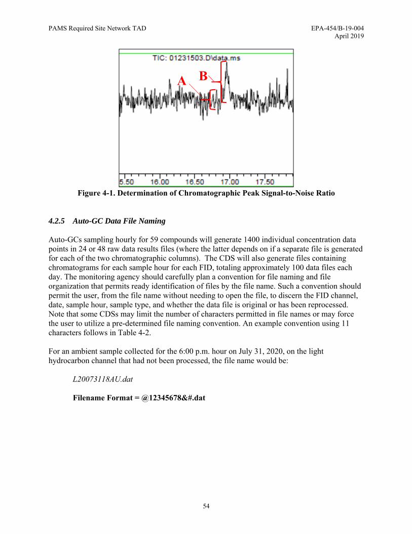
PAMS Required Site Network TAD EPA-454/B-19-004 April 2019
54
Figure 4-1. Determination of Chromatographic Peak Signal-to-Noise Ratio
4.2.5 Auto-GC Data File Naming Auto-GCs sampling hourly for 59 compounds will generate 1400 individual concentration data points in 24 or 48 raw data results files (where the latter depends on if a separate file is generated for each of the two chromatographic columns). The CDS will also generate files containing chromatograms for each sample hour for each FID, totaling approximately 100 data files each day. The monitoring agency should carefully plan a convention for file naming and file organization that permits ready identification of files by the file name. Such a convention should permit the user, from the file name without needing to open the file, to discern the FID channel, date, sample hour, sample type, and whether the data file is original or has been reprocessed. Note that some CDSs may limit the number of characters permitted in file names or may force the user to utilize a pre-determined file naming convention. An example convention using 11 characters follows in Table 4-2. For an ambient sample collected for the 6:00 p.m. hour on July 31, 2020, on the light hydrocarbon channel that had not been processed, the file name would be: L20073118AU.dat Filename Format = @12345678&#.dat
A B

PAMS Required Site Network TAD EPA-454/B-19-004 April 2019
55
Table 4-2. Example Auto-GC File Naming Convention
Position Detail Character or Character Combination @ Hydrocarbon channel L = light HC channel
H = heavy HC channel1 & 2 2-digit year (YY) 2-digit numeric3 & 4 2-digit month (MM) 00 through 125 & 6 2-digit day (DD) 00 through 317 & 8 2-digit hour from 24-
hour clock 00 through 23
& Sample type A = ambient sample B = blank sample C = continuing calibration verification (CCV) I = initial calibration standard P = precision check standard S = second source calibration verification (SSCV) X = exploratory or experimental (troubleshooting, conditioning, etc.)
# Processing status U = unprocessed R = reprocessed
4.3 Method Detection Limits for Auto-GC Annually prior to each PAMS sampling season, PAMS Required Site monitoring agencies should determine the MDL of each priority compound and optional compound. MDLs are needed to provide method sensitivity information to the data user. The EPA auto-GC studies conducted to determine instruments suitable for PAMS Required Site deployment demonstrated that an MDL of 0.5 ppbC or less could be achieved for most target compounds.4,5 Discussions with auto-GC operators have indicated that the selected auto-GC instruments are capable of detecting lower concentrations, in some cases as low as 0.1 ppbC. Briefly, MDLs are determined per the MUR of the MDL process defined in 40 CFR Part 136 Appendix B,20 which prescribes that a minimum of seven low-level standards and seven blanks be prepared in the matrix and analyzed. The average concentration and the standard deviation of the standard analyses and blank analyses are calculated separately and used to generate the MDL values. The instrument should be calibrated and pass all relevant quality control criteria before analysis of MDL samples. When conducting the MDL study, auto-GC operators are encouraged to ensure that the instrument and support equipment have been operating and stable for several weeks. This includes ensuring that the preconcentrator trap has been conditioned to ensure quantitative adsorption and desorption and to minimize and preferably eliminate interferences, and that the humidified matrix blank background levels are sufficiently low. This warm-up and conditioning period further ensures that support equipment such as zero air generators, hydrogen generators,

PAMS Required Site Network TAD EPA-454/B-19-004 April 2019
56
and gas purifiers are functioning properly and that gas delivery pathways have been flushed and properly conditioned. Once the instrument conditioning and stabilization are complete, calibration can be established for the two FIDs. Matrix blanks and spikes for determining the MDL are analyzed over the course of three or more different non-consecutive days. Distributing the blank and standard analyses over time incorporates a component of temporal variability in the MDL determination and increases the representativeness of the auto-GCs routine performance. While the conduct of the MDL itself is different, the example calculation shown in Section 5.6.2 for determining carbonyls MDLs is analogous to determination of MDLs for speciated VOCs by auto-GC. 4.3.1 MDL Blank Component, MDLb For the blank component of the MDL, operators should include in the calculation those humidified blanks analyzed with the instrument after completing shakedown and achieving stabilization. While operators should make reasonable efforts to ensure the instrument is clean and target analyte responses are as low as possible, it is normal to see some background of target analytes in chromatograms. Blanks that show typical concentrations of target compounds should not be excluded from the MDL calculation; however, if the concentrations of these compounds appear to be decreasing over time and continue to decrease, the system may not be completely stable with respect to contamination levels, and may require a longer stabilization period before generating blank data for use in the MDL determination. Inclusion of only typical blank background levels is important to determine a realistic MDL. Each auto-GC performs uniquely, and levels of background for one instrument may be different for another separate but identical auto-GC. For contamination in blanks which is excessive (~0.3 ppbC or above, analyte dependent), operators should take corrective actions to eliminate the source and root cause of the contamination where possible before analyzing blanks to include in the MDL calculation. It is acceptable to exclude blanks from the MDL calculation for technical reasons, such as blanks that are known to be problematic due to instrument issues such as uncharacteristic contamination or memory effects (e.g., blanks analyzed following a high concentration calibration standard). A minimum of seven humidified blank analyses is needed to calculate the MDLb; however, operators should include as much typical blank data as possible to provide a realistic average background concentration (and its associated variability) to generate the MDLb. 4.3.2 MDL Standard Spike Component, MDLsp To determine the standard spike component of the MDL, matrix standard concentrations of the target analytes are chosen to be analyzed minimally seven times. If too low of a spiking level is chosen, the analyte may not be reliably detected. If too high of a spiking level is chosen, the variability of the method near the actual limits of detection may not be properly characterized. An appropriate spiking level may be selected by considering the following (in order of importance):
1. The concentration at which the instrument S:N is three- to five-fold for the analyte. Auto-GC operators in November 2017 indicated that diluting the stock RTS (15 to 60 ppbC) to 100-fold (0.15 to 0.6 ppbC) and 200-fold (0.075 and 0.3 ppbC),

PAMS Required Site Network TAD EPA-454/B-19-004 April 2019
57
respectively, provided analyte responses at approximately a S:N of 5:1 for the heavy and light HCs, respectively.
2. The concentration at which qualitative identification criteria for the analyte are lost (note that this will be a S:N below approximately 5:1 and will be approximately the concentration determined from the MDL process absent of blank contamination).
3. Analysis of a suite of matrix blank samples; calculate the standard deviation of the measured concentration and multiply by 3.
4. Previously acceptable MDL studies and related experience.
Note that the MDL spiking level should not be within the calibration curve (which will typically span approximately 1 to 25 ppbC); rather, the MDL spiking level should be less than the lowest calibration standard in order to determine the most realistic MDL. Concentrations within the calibration curve are required to meet method precision and bias acceptance criteria and are of a sufficient concentration that qualitative identification is certain, which practical experience has shown to be approximately three- to five-fold the expected MDL concentration. MDL standard spikes are typically analyzed from the RTS (or a similar standard) which contains most of the target analytes. Concentrations of target analytes in the RTS typically range from tens of ppbC to approximately 50 ppbC, therefore, as described above, the RTS may require two or more different dilution ratios to achieve a concentration of 0.5 ppbC for each target analyte. Alternatively, a standard gas prepared with all target compounds at the same concentration in ppbC (e.g., 100 ppbC) can be readily diluted to approximately 0.5 ppbC for determining MDLs. Preparation of the chosen concentrations and introduction of the standards to the instrument may be performed by one of several conventions, depending on the equipment available at the site. In all cases, the standards analyzed to determine the MDL will need to be humidified to ensure proper performance of the higher molecular weight (C9 and C10) target compounds. Analysis of dry gas standards will result in MDLs that are not representative of those expected to be achieved in ambient air (which always contains some amount of moisture during the PAMS season) and may result in depressed target compound response for some analytes. To generate representative MDL standards, they should be prepared in a similar convention to the instrument calibration standards, which may include:
1. Preparation of a standard canister at the desired concentration(s): The RTS is diluted to the desired concentration with humidified zero air into a clean evacuated stainless steel canister. Dilution may be performed by static dilution (refer to Section 4.5.2.1) or dynamic dilution (refer to Section 4.5.2.2). Dilution into a canister has several drawbacks as the inclusion of the canister in the MDL process can impart bias (positive or negative) depending on the target compound under evaluation and the condition or cleanliness of the canister. Recovering target hydrocarbon analytes from canisters can be problematic, particularly C9 and C10 compounds with higher boiling points. Standards prepared in canisters should be properly humidified (~ 40 to 50 % RH) to ensure recovery of higher molecular weight compounds from the canister. Humidification is discussed further in Section 4.5.2.4.

PAMS Required Site Network TAD EPA-454/B-19-004 April 2019
58
Monitoring agencies should note that the absolute accuracy of the standard gas dilution for MDL determination is not critical, as the MDL procedure is designed to characterize the variability of replicate analysis at approximately the MDL concentration. Prior to the use of canisters, users are encouraged to verify that the canister(s) impart acceptably low bias by performing a bias check on the canister (further information on performing bias checks on canisters can be found in Revision 3 of the NATTS TAD, available at the following link on AMTIC: https://www3.epa.gov/ttnamti1/files/ambient/airtox/NATTS%20TAD%20Revision%203_FINAL%20October%202016.pdf). Note that the determination of canister bias is not critical if all MDL standards are taken from the same canister. However, if a number of canisters is employed, use of uncharacterized canisters may impart additional variability to the MDL process and result in artificially elevated determined MDLs. Active sites within canisters can result in the low recovery of labile analytes such as acetylene, olefins, and terpenes. An additional drawback to preparing standards in canisters is that there is a limited number of samples that can be drawn from the canister before the canister pressure is insufficient for the auto-GC to remove a sample aliquot. In such instances, another standard canister will need to be prepared. In general, use of canisters for preparing standards requires a support laboratory with the capability to perform heated canister cleaning and evacuation. Note: Unlike canister collection methods, preparation of MDLs for auto-GCs does not require that a minimum of seven separate canisters be prepared. The requirement for canister collection methods to include a minimum of seven separate canister samples does not apply to auto-GCs as the measurement method does not utilize a canister for sample collection and therefore does not require characterization of the variability inherent in the canister fleet.
2. Pulsed standard delivery: The RTS is connected directly to the instrument inlet and “pulsed” to deliver the standard for a known portion of the 40-minute sampling duration. Instrument operators should note that reproducible delivery is more difficult to achieve when employing short pulse times (e.g., less than 4 minutes) due to the increased variability in MFC performance during startup and shutdown, and that MDLs determined in this manner may be biased high as a result. The remaining duration of the 40-minute sampling period should consist of sampling humidified zero air to best replicate the humidity exposure to the system during routine analyses. Refer to Section 4.5.2.3 for further information and an example calculation for pulsed standard delivery.
3. Delivery of a dynamic dilution gas stream to the instrument: The RTS is diluted with humidified zero air to achieve the desired concentration and this diluted gas is delivered to the auto-GC for analysis as described in Section 4.5.2.2. The auto-GC samples the gas stream for the entire 40-minute sampling period as is done for calibration standards, ambient samples, and blanks. This convention replicates the manner in which ambient air

PAMS Required Site Network TAD EPA-454/B-19-004 April 2019
59
is introduced to the auto-GC and is likely to result in the most representative and accurate MDLs. The main drawbacks to this convention are that it requires additional equipment (a dynamic dilution gas calibrator system) and is less conservative of standard gas consumption than either delivery of MDL standard aliquots by canister or by pulsed standard delivery.
The EPA anticipates development of a subscription service through which the RTS will be available at an approximate 10-fold dilution (approximately 1.5 to 6 ppbC per target compound) with which MDL standards may be prepared. Instrument operators will analyze the standard in a pulsed fashion (as described in paragraph 2 above) to provide an effective dilution to the auto-GC and complete the sampling with humidified zero air.
4.3.3 Redetermination of MDLs
MDLs are to be determined annually prior to the beginning of each PAMS season and when there are changes to the auto-GC that would reasonably result in changes in its sensitivity. For MDL determination prior to PAMS season, it is recommended that MDLs be determined following the typical annual instrument maintenance which should include replacing the preconcentrator trap and Nafion™ dryer (if so equipped). As discussed in Section 4.2.3.3, the auto-GC should be conditioned for several weeks to ensure that the instrument is sufficiently clean and that its performance is stable. Once sufficiently conditioned, FID response is typically stable over time, and a decrease in propane, butane, or benzene response factor that exceeds 10% from the initial calibration indicates a decrease in sensitivity that may require preconcentrator trap replacement or other system maintenance. Such a decrease in response would typically occur over a longer period than the three-month PAMS season, even including the several weeks of conditioning prior to beginning monitoring for the year. If, after such trap replacement or maintenance, the response factor returns to within 5% of that level determined in the initial calibration (by analysis of a standard with a concentration in the lower third of the calibration curve), the MDL would not require redetermination. If the response factor remains depressed as compared to the initial calibration, the MDL should be determined anew following recalibration of the instrument. 4.4 Auto-GC Interferences Approved auto-GCs for use at PAMS Required Sites range from instruments specifically designed for field use to laboratory instruments configured to operate in a monitoring shelter. For any of the instrument systems, they can be subject to interferences which impact measurement quality. The most common interferences result from the presence of ozone and/or moisture and fluctuations in shelter temperature. 4.4.1 Ozone Interference During sample preconcentration, co-collected ozone may react with target analytes (particularly unsaturated hydrocarbons) within the air stream, with target analytes trapped on the sorbent beds, and with the sorbents themselves. Such reactions result in the formation of oxidized organic byproducts that may appear as unknown peaks in the chromatogram. To date, ozone scrubbers are prescribed for carbonyl sampling (as discussed in Section 5.4) but have not been formally

PAMS Required Site Network TAD EPA-454/B-19-004 April 2019
60
evaluated with the approved auto-GC systems and have not been widely adopted for removing ozone interferences from the analysis of VOCs by auto-GC. Use of an ozone denuder on auto-GC inlets is not recommended unless the monitoring agency has performed an appropriate collocation study to evaluate effects of the ozone denuder on the ambient measurements. Such a study would require passing calibration standards and QC samples through the ozone denuder. Further detail of such a collocation study is outside the scope of this TAD. 4.4.2 Moisture As discussed in Section 4.2.3.2, water vapor can adversely impact auto-GC performance. Sampled gas streams that are insufficiently dehydrated prior to reaching the preconcentrator traps can result in trap icing and/or poor chromatography and RT shifts of target analytes. Moisture from insufficiently dried carrier gases can have similar effects on chromatography and RTs. Such changes in chromatography can persist in the light hydrocarbon column for several consecutive runs. Moisture remaining on preconcentrator traps when the thermal desorption step begins can degrade sorbents and water introduced onto the separation columns can damage stationary phase linings. Preconcentration systems typically perform a purge of the preconcentrator trap with dry carrier gas at the end of the sample collection prior to trap heating for desorption. The flow rate and volume of this dry purge is selected to provide sufficient dehydration while minimizing the loss of target analytes retained on the trap. 4.4.3 Temperature Auto-GCs are sensitive to temperature fluctuations within the monitoring shelter. Monitoring shelters for auto-GCs require heating, ventilation, and air conditioning (HVAC) systems to maintain environmental conditions suitable for instrument operation. During the June 1 through August 31 PAMS season, shelters will typically require air conditioning to maintain shelter temperatures below ambient. Auto-GC moisture management systems employing NafionTM dryers are more effective at lower temperatures. Temperature fluctuations in the monitoring shelter can cause insufficient drying of the ambient air and/or humidified check standard gases and may result in excess moisture passing through to the preconcentrator trap and/or GC column(s). As PAMS Required Sites are typically located at NCore sites, PAMS instruments may be installed with criteria gas monitoring instruments in shelters that are required to be maintained at 20 to 30°C with a standard deviation of ≤ 2% over 24 hours. These conditions are sufficient for auto-GC installation; however, existing HVAC systems may be of a capacity insufficient to maintain conditions with the additional heat burden from the PAMS instruments. In such cases where criteria pollutant monitors and PAMS instruments can be installed in the same shelter, additional cooling capacity may be required or partitions can be installed either to maintain environmental conditions for the criteria pollutant monitors or to stabilize the environmental conditions for the auto-GC. The auto-GC, its support equipment, and its exhausts should be placed sufficiently away from HVAC thermostats to ensure the latter do not artificially influence HVAC operation. If auto-GCs are installed in separate shelters from the criteria pollutant monitors, recommendations in the following paragraphs should be considered. Efficient chromatographic separation is accomplished by ramping the temperature of the GC column from approximately 30°C to 200°C. Following the completion of the temperature ramp,

PAMS Required Site Network TAD EPA-454/B-19-004 April 2019
61
the oven temperature is reduced through venting to achieve the initial temperature for analysis of the next sample. Achieving reproducible and predictable compound RTs requires precise control of the oven temperature; however, shelter temperature fluctuations can result in changes in the GC oven temperature profile during analysis with consequent changes in observed RTs. It may be difficult for auto-GCs in monitoring shelters with insufficient cooling capacity to return to the starting oven temperature or for the Peltier cooler in the thermal desorber or dryer to reach its initial temperature setpoint. In such cases, the thermal desorber may not be ready to collect the sample at the proper time or the GC portion of the instrument may not be ready to begin separation of the collected sample when the thermal desorber is programmed to introduce the sample to the GC, ultimately causing a cascade of delays within the instrument and preventing sample analysis per the intended hourly schedule. Additionally, auto-GCs in shelters that experience higher temperatures may experience shortened Peltier cooler life due to the additional cooling burden required to reach its initial temperature setpoint. It is recommended that monitoring agencies consult with an HVAC professional to ensure the monitoring shelter’s cooling capacity is sufficient. Several of the auto-GC instruments incorporate connections on the GC oven vent to permit routing oven heat exhaust to the exterior of the shelter, reducing cooling demand for the HVAC system. Additionally, locating compressors for zero air generation systems outside the monitoring shelter (protected from the elements) will reduce both heat burden and noise levels inside the shelter. Installation of compressors outdoors will require more frequent maintenance due to increased humidity in the source air and the build-up of water in the compressor ballast tank(s). To reduce temperature fluctuations at the instrument to the extent possible, avoid direct impingement of conditioned air onto the auto-GC. This can be accomplished by installing baffles to diffuse flows of conditioned air and/or redistributing HVAC outlets to reduce temperature gradients within the monitoring shelter. 4.4.4 Source-Oriented Interferences Monitoring sites that are impacted by industrial sources, such as refineries, refueling stations, or other similar sources, may contribute unknown hydrocarbon artifacts to the GC chromatogram, particularly on the heavy hydrocarbon (PDMS column) channel. These additional hydrocarbons may produce interfering peaks in chromatograms that coelute with target compounds and complicate the integration and identification of target analytes. Where chromatographic resolution is inadequate, the amount of area integrated for the target peak will typically be defined by a vertical to the baseline and the resulting area will be less than that for a completely resolved peak. In such instances, the instrument operator should indicate the reported concentration is biased low and qualify the concentration as “LL” when reporting it to AQS. In some cases coeluting peaks will be larger than the target analyte peak, especially when the target peak is a small shoulder on the coeluting compound. In such cases, the instrument operator and technical reviewers should evaluate whether the value should be estimated or invalidated.

PAMS Required Site Network TAD EPA-454/B-19-004 April 2019
62
4.4.5 Problematic Compounds for Auto-GC Target compounds that are particularly problematic with respect to recovery are acetylene (C2H2), styrene (C8H8), and alpha- and beta-pinene (C10H16). Acetylene typically shows lower recovery (70% or less) when compared to the other light hydrocarbons when analyzed as part of a CCV. While the low recovery problem is well-documented for acetylene21 the reasons for this lower recovery appear to be due to a combination of instability of acetylene within the high-pressure stock standard cylinders and the inability to quantitatively trap and desorb acetylene. Styrene is suspected to be unstable in the high-pressure stock standard cylinder; however, experience has shown that trapping and desorbing styrene is not particularly problematic. Lower recoveries of styrene have been reported when establishing calibrations based on the carbon response of benzene and when analyzing CCVs. These lower recoveries are typically consistent with concentrations relative to other species in the standard mixture, even over the course of several months to a year, indicating that the concentration of styrene has decreased then stabilized within the standard cylinder. For alpha- and beta-pinene, the beta isomer is suspected to be unstable in the high-pressure stock standard cylinder, with the latter typically isomerizing to form camphene, d-limonene and/or alpha-pinene. While alpha-pinene appears to be more stable than the beta isomer, the former may also isomerize or decompose. Losses of both pinenes will manifest as changes in their response relative to the other target compounds in the standard cylinder, particularly the compounds propane and benzene employed to establish the FID carbon responses. Monitoring agencies should be aware that acetylene, styrene, alpha-pinene, and beta-pinene may not meet the established bias criteria (±30% difference from the theoretical concentration) in routine QC samples even on recently calibrated and stabilized auto-GC instruments with new preconcentrator traps. In such instances, ambient concentration data for these monoterpenes should be appropriately qualified as an estimate (refer to Table 11-2). More information on the stability of monoterpenes in cylinders may be found elsewhere.22 Monitoring agencies should also note that three compounds listed in Table 4-1 (optional compounds) are not included in the RTS typically sourced by EPA: carbon tetrachloride (halogenated), tetrachloroethylene (halogenated), and ethanol (alcohol). Each of these compounds responds differently (less intensely) to an FID than hydrocarbons and each will likely not demonstrate expected accuracy (±30% of nominal) using a carbon-based response factor. In addition to the decreased FID response relative to hydrocarbons, monitoring agencies operating auto-GCs with NafionTM sample stream drying systems will be unable to accurately determine ethanol concentration as the fluoroelastomer polymer membrane removes a fraction of ethanol from the sampled air stream.

PAMS Required Site Network TAD EPA-454/B-19-004 April 2019
63
4.5 Calibration of Auto-GCs 4.5.1 Standard Materials Stock standards for calibration of the auto-GC are commercially available. Standard gases will preferably be National Institute of Standards and Technology (NIST)-certified or NIST-traceable certified and are to be accompanied by a certificate of analysis stating the certified concentration and associated uncertainty for each component. Expiration dates are typically one year or more and several vendors offer a recertification service that verifies the component concentrations and extends the useful life of the standard cylinder beyond the original expiration date. Recertification of standard gases is often more cost effective than purchasing new standards and can be performed during the non-sampling season (as applicable to the specific PAMS Required Site). Note that manufacturers may exclude the compounds note in Section 4.4.5 from their guarantee of stability. 4.5.1.1 Primary Calibration Standard The standard chosen for calibration, the primary calibration source, is to minimally be NIST-traceably certified for propane or butane and benzene. The primary calibration source will typically be a high-pressure cylinder minimally containing two compounds, propane and benzene, but if the auto-GC permits, the source may be from NIST-traceably certified permeation tubes of target compounds (one for each FID channel), such as butane and benzene. It may be useful for troubleshooting purposes to include other target compounds in the primary calibration stock gas, such as a suite of compounds representing the C2 to C10 range, the priority compounds, or other combination of desired target compounds. Several gas vendors offer an 18-component blend, mimicking the previously available NIST 1800b standard, and containing the following analytes:
ethane n-hexanepropane n-heptanepropene benzeneiso-butane iso-octanen-butane n-octaneiso-butene tolueneiso-pentane nonanen-pentane o-xylene1-pentene decane
Selection of standard concentrations depends on the capability of the operator to dilute the standard with humidified zero air to generate concentrations in the desired range calibration range of 1 to 25 ppbC. 4.5.1.2 Secondary Source Calibration Verification Standard The calibration established by analysis of the primary calibration standard will be verified by analysis of second source calibration verification standard (SSCV). The SSCV stock standard will typically be the PAMS RTS and will contain all of the priority and many of the optional compounds (Note: The current PAMS RTS contains 59 compounds and includes all priority

PAMS Required Site Network TAD EPA-454/B-19-004 April 2019
64
speciated VOCs and most of the optional speciated VOCs with the exceptions of carbon tetrachloride, tetrachloroethylene, and ethanol; Refer to Table 4-1. The RTS is prepared to contain the target analytes at concentrations covering approximately 15 to 60 ppbC.) The SSCV stock will be sourced from a different provider than the primary calibration standard or will minimally be from a different lot of source material from the same provider, if unavailable from an independent supplier. The SSCV stock standard is to minimally be NIST-traceably certified for propane or butane and benzene to verify the calibration established with the primary standard. The recoveries of the other target VOCs will be evaluated by analysis of the SSCV. The SSCV is prepared from this standard at a concentration within the lower third of the calibration curve (approximately 5 ppbC for propane or butane and benzene). Acceptance criteria are listed in Table 4-4. 4.5.1.3 Retention Time Standard In order to establish RT windows for each of the target analytes, a known standard is to be analyzed on the auto-GC to determine the RT of the individual target compounds. The RTS described in Section 4.5.1.2 serves this purpose. Two compounds included in the RTS blend but not listed among the target analytes in Table 4-1 are 1-hexene and dodecane, which are used to set Deans switch timing and end the GC run, respectively. EPA supplies the RTS to PAMS sites and has provided for the RTS to be NIST-traceable certified for propane and benzene. As such, when certified for these two compounds, the RTS may also serve as the SSCV (see Section 4.5.1.2). If not employed as the CCV or SSCV, there are no recovery criteria associated with the RTS since its purpose is to verify and adjust target analyte RTs, and not to evaluate the calibration response. 4.5.1.4 Zero Air Zero air is not a standard gas; however, it is critical for the proper performance of the auto-GC, specifically to demonstrate lack of interferences in system blanks and to prepare non-biased and reproducible dilutions of stock standards. Zero air is also typically employed as the oxidizer for the hydrogen fuel in FIDs, as the purge gas for dehydrating sample streams with NafionTM dryers, and/or as the purge gas to prevent moisture from freezing on the Peltier coolers in electronic sample dryers and preconcentrators. The zero air should be provided by an online zero air generator (ZAG) that can generate approximately 5 L/minute flow of nominally HC-free air (total hydrocarbon concentration of ≤ 10 ppbC, and preferably less). When employed as dry gas for sample stream dehydration or Peltier purging, zero air should have a dewpoint of ≤ -100°C. Zero air employed for diluting standard gases and/or as zero air blanks should be humidified to approximately 40-50% RH. For zero air generation systems providing both gas for dry purging and for the QC sample matrix (standards dilution or blank), the humidification for QC samples should occur downstream from the dry gas split. Dry nitrogen, such as available in high-pressure cylinders, may be substituted for zero air employed as the dry purge gas. Such a substitution requires the monitoring agency to replace nitrogen cylinders routinely and does not eliminate the need for zero air for FIDs and for use as a QC sample matrix. For sites employing zero air as a purge gas, dry nitrogen or dry zero air in a high-pressure cylinder may be useful for troubleshooting a ZAG’s water removal capability.

PAMS Required Site Network TAD EPA-454/B-19-004 April 2019
65
ZAGs providing zero air for blank analysis and as a diluent should be evaluated to ensure the generated gas is sufficiently clean. ZAGs should be set up, conditioned, and operated per the manufacturer’s instructions prior to connection to the auto-GC sample inlet or to a dilution system. This permits flushing of any contaminants in the ZAG system that could otherwise contaminate the instrument(s). Once the proper conditioning has been completed, an aliquot of the zero air should be analyzed and evaluated to ensure the concentrations of target analytes and interferences are sufficiently low (minimally < 0.5 ppbC for each compound to be reported to AQS, and preferably very little chromatographic peak response on either channel – total hydrocarbons < 10 ppbC). In general, a chromatogram of zero air should show little or no response for target analytes. Where concentrations of reportable compounds exceed ≥ 0.5 ppbC, the ZAG should be disconnected from sampling inlets and dilution systems and permitted longer periods of flushing, or subjected to maintenance prior to redeployment. 4.5.2 Retention Time Establishment and Calibration Convention and Procedure Prior to attempting to calibrate the auto-GC prior to the beginning of PAMS season, the operator should first verify that instrument maintenance has been performed to replace the preconcentrator trap and the NafionTM dryer (if so equipped) and to verify the instrument is functioning properly (e.g., no error messages, the instrument progresses through a sequence normally, etc.). It is also recommended that the operator assess the need to replace carrier gas scrubbers and ZAG consumables as this ensures optimum auto-GC performance and reduces the likelihood that future troubleshooting may be required. The instrument should be powered on and analyzing ambient air or humidified zero air for minimally two weeks (preferably longer) to ensure the instrument is leak-free and operating properly and that the support equipment (compressors, zero air generator(s), hydrogen generator, etc.) is functioning properly. During this time, it is suggested that the trap conditioning described in Section 4.2.3.3 be conducted. For monitoring agencies operating year-round that cannot afford several weeks of instrument down time, the conditioning period may be shortened, as needed, so long as ongoing demonstration of instrument performance is attained. Once it is established that the instrument is operating properly, the operator should analyze a series of humidified blanks to ensure there are no chromatographic artifacts and that the instrument is sufficiently clean. If the preconcentrator trap has recently been replaced, levels of contaminant target compounds in the humidified zero air blank may still be desorbing from the trap, and the conditioning should continue until target compound concentrations are acceptably low. The instrument is sufficiently clean when there are few and very small chromatographic peaks in the blank chromatograms and the target compound responses in the humidified zero air blanks are stable and do not exceed 0.5 ppbC. Following successful demonstration that the instrument is appropriately clean, the operator should analyze the humidified RTS a minimum of five times successively to establish and assign retention windows for the target analytes. The mean, standard deviation, and percent relative standard deviation (RSD) of the RTs for each compound should be calculated for the five aliquots. If the percent RSD of the mean RT exceeds 5% for any compound, the RT may not stable for that compound and/or the peak identification may not be correct. If peak identifications are correct, the instrument operator should analyze additional RTS aliquots until the RTs stabilize (RT RSDs < 5%).

PAMS Required Site Network TAD EPA-454/B-19-004 April 2019
66
RSD is calculated by dividing the standard deviation of the population of measurements population by the arithmetic mean of the population, expressed as a percentage:
% ∙ 100%
where: σ = standard deviation of population = population arithmetic mean Once the RT windows have been established and are stable for the target analytes, a series of humidified zero air blanks is again analyzed and the operator again verifies the instrument is acceptably free of contaminants and carryover. Once the auto-GC is demonstrated to be acceptably clean, the operator can calibrate the instrument. The instrument calibration is to include a minimum of three standard levels at approximately 1, 5, and 25 ppbC for propane or butane and benzene. The propane or butane responses will be used to establish the carbon-based response calibration for the light HC “PLOT” FID channel and the benzene responses will be used to establish the carbon-based response for the heavy HC “PDMS” FID channel. As discussed above in Section 4.5.1.1, the primary calibration source gas(es) are to be NIST-traceably certified for minimally propane or butane and benzene. If the primary calibration gases are sourced from high pressure cylinders, the standards may be introduced by the following conventions (as described in Section 4.3.2):
dilution of stock standard gas into a canister or canisters for introduction to the auto-GC (Note: canisters used for this purpose will need to be appropriately qualified and cleaned for this use.)
dynamically diluting a stock gas using differential flow control to actively deliver a known concentration gas to the auto-GC
pulsing delivery of a stock standard gas to introduce known masses of standard (equivalent to that contained in the typically-collected volume of gas at the three challenge concentrations) to the preconcentrator
Auto-GC systems employing permeation tubes for generating calibration standard levels will establish calibration by delivering known masses to the preconcentrator based on the dilution of the gas evolved from the permeation tube, where the masses are determined as with the pulsed delivery method. Permeation tubes are maintained in a temperature-controlled oven and emit a known mass of the target compound at a known rate at a given constant temperature. 4.5.2.1 Static Dilution Static dilution of a gas standard can be performed by adding known amounts of a standard gas and diluent gas to a fixed volume vessel (such as a canister) and measuring their partial pressures with a calibrated pressure gauge or transducer. The technician should establish a desired final

PAMS Required Site Network TAD EPA-454/B-19-004 April 2019
67
pressure and desired final concentration of the target compounds as well as the corresponding volumes of standard and diluent gas prior to beginning the dilution process. Starting with an evacuated canister (initial vacuum of ≤ 0.5 psia), the pressure is measured with a calibrated pressure gauge or transducer and recorded. Next a standard gas is connected to the canister and the gas slowly added to the canister to the desired pressure and the pressure permitted to stabilize. This pressure is measured and recorded with a calibrated gauge. Finally, humidified diluent gas is added to the canister to the desired final pressure to complete the dilution. The following is an example for static standard preparation of a 25-ppbC propane and benzene: Example Static Dilution:
Primary Stock Gas: 507 ppbC propane and 495 ppbC benzene Desired Working Standard Concentration: 25 ppbC Fixed Vessel: 6-L stainless steel canister Final Desired Absolute Pressure: 30 psia 1. Calculate the effective dilution factor (DF) needed by dividing the stock gas
concentration by the desired working standard concentration (these concentrations can be approximate to determine the DF):
500 ppbC/25 ppbC = 20
2. For a 20-fold dilution and a final pressure of 30 psia, it is assumed the canister has been evacuated to hard vacuum of 0 psia and the required partial pressures of the stock gas can be calculated by dividing the final desired absolute pressure by the DF:
30 psia/20 = 1.5 psia
3. The evacuated canister pressure is measured to be 0.50 psia. Note that to minimize contamination from previous canister contents, the evacuated canister pressure will ideally be ≤ 0.1 psia (> 29.7 in Hg vacuum). If the intended diluent gas is not humidified, the canister can be humidified at this time. Refer to Section 4.5.2.4 for further information on humidification.
4. The stock calibration gas is connected via a regulator to the canister. The stock gas is then bled into the canister until 1.5 psia has been added to the canister. Since the canister starting pressure was 0.50 psia, the pressure gauge will read 2.0 psia. The canister pressure reading is allowed to stabilize, the pressure recorded, the valve is closed, and the calibration gas is disconnected.
5. The diluent gas (humidified zero air) is then connected to the canister and bled into the canister to the desired final pressure (30 psia) and the pressure measured once the pressure stabilizes as 30.4 psia. The canister valve is then closed and the standard

PAMS Required Site Network TAD EPA-454/B-19-004 April 2019
68
preparation is complete. The canister is then held overnight prior to use to stabilize.
6. The final nominal concentration of the diluted standard is calculated as follows:
∙
where:
Cfinal = final nominal concentration of the target compound (ppbC) Cstock = stock gas concentration of target compound from certificate of
analysis (COA) (ppbC) Pstock = pressure of stock gas added to the vessel (psia) Ptotal = final total pressure of the vessel (psia)
7. For this example:
Cstock = 507 ppbC propane and 495 ppbC benzene Pstock = 1.5 psia Ptotal = 30.4 psia
Propane Cfinal = 507 ppbC · 1.5 psia = 25.0 ppbC 30.4 psia
Benzene Cfinal = 495 ppbC · 1.5 psia = 24.4 ppbC 30.4 psia
4.5.2.2 Dynamic Dilution Dynamic dilution is a method of preparing a known standard gas by admitting known volumetric flows of stock standard gas(es) and a diluent gas into a mixing chamber. This method typically employs calibrated mass flow controllers or mechanical valves or restrictors with associated calibrated pressure transducers to control the standard and diluent gas flows. The standard and diluent gases should be flowing at the desired rates for a sufficient time to permit complete passivation of the dilution apparatus flow paths. Passivation timing is dependent on the mixing chamber volume and total gas flows, but systems should be passivated for minimally five minutes when diluting gases with lower boiling points (such as a two-component propane and benzene standard). This passivation period is of particular importance when diluting high boiling point VOCs (such as C9 and C10 compounds) and should be minimally 30 minutes in such cases. Exhausts should be directed to a fume hood or snorkel. As with static dilution, the technician should establish the desired final concentrations of the target compounds and be familiar with the flow range limitations of the flow control devices prior to beginning the dilution process. For example, most mass flow controllers operate optimally within 10 to 90% of their full-scale rating (e.g., a 1000 cc/minute MFC should be operated between 100 to 900 cc/minute) and may not control flow well outside this range. The flows of the stock standard gas and the diluent gas are set to provide the desired DF. If a

PAMS Required Site Network TAD EPA-454/B-19-004 April 2019
69
minimum flow rate is required for delivery of the diluted gas to the auto-GC inlet, this should be considered when setting the flow rates. Dynamically diluted standards may be delivered directly to the auto-GC inlet or may be delivered for capture in an evacuated canister. Diluent gases should be humidified to ensure proper quantitative transfer of all target species. Refer to Section 4.5.2.4 for information on humidification. The following is an example for dynamically preparing a 25 ppbC standard of propane and benzene: Example Dynamic Dilution:
Primary Stock Gas: 512 ppbC propane and 492 ppbC benzene Desired Working Standard Concentration: 25 ppbC Minimum Required Flow Rate: 45 mL/minute Standard Gas Flow Controller Range: 0 to 100 mL/minute Diluent Gas Flow Controller Range: 0 to 5000 mL/minute
1. Calculate the effective DF needed by dividing the stock gas concentration by the
desired working standard concentration (these concentrations can be approximate to determine the DF):
500 ppbC/25 ppbC = 20
2. For a 20-fold DF, the flow controllers will need to be within their recommended
operating ranges. To determine the total flow rate needed, multiply the standard flow controller range minimum (10% full scale, or 10 mL/min) and maximum (90% full scale, or 90 mL/min) by the dilution factor.
10 mL/minute · 20 = 200 mL/minute 90 mL/minute · 20 = 1800 mL/minute
3. Verify that the total flow exceeds the required minimum flow (preferably this
would be exceeded by a factor of 2). The minimum total flow rate of diluted gas of 200 mL/minute exceeds 45 mL/minute, so the total flow rate will be adequate for any selected rate of delivery of standard gas.
4. Calculate the flow rate range of the diluent channel by subtracting the standard flow needed at the minimum and maximum potential flow rates for the standard gas from the minimum and maximum total flows required to achieve the DF (from step 2).
200 mL/minute – 10 mL/minute = 190 mL/minute 1800 mL/minute – 90 mL/minute = 1710 mL/minute

PAMS Required Site Network TAD EPA-454/B-19-004 April 2019
70
The minimum diluent flow is 500 mL/minute (10% full scale), therefore the diluent flow must be between 500 and 1710 mL/minute. To conserve standard gas, choose a total flow close to, but above the minimum, e.g., 600 mL/minute.
5. Determine the approximate needed standard flow corresponding to a diluent flow
of 600 mL/minute, by dividing the diluent flow by the DF:
600 mL/minute /DF = 600 mL/minute /20 = 30 mL/minute
6. Determine the needed diluent flow for a standard flow of 30 mL/minute by subtracting the standard flow from the total flow:
600 mL/minute – 30 mL/minute = 570 mL/minute
7. The final nominal concentration of the diluted standard is calculated as follows:
∙
where:
Cfinal = final nominal concentration of the target compound (ppbC) Cstock = stock gas concentration of target compound from COA (ppbC) Fstock = calibrated flow of standard gas (mL/minute) Fdiluent = calibrated flow of diluent gas (mL/minute)
8. For this example:
Cstock = 512 ppbC propane and 492 ppbC benzene Fstock = 30 mL/minute Fdiluent = 570 mL/minute
Propane Cfinal = 512 ppbC · 30 mL/minute = 25.6 ppbC 570 mL/minute + 30 mL/minute
Benzene Cfinal = 492 ppbC · 30 mL/minute = 24.6 ppbC
570 mL/minute + 30 mL/minute 4.5.2.3 Pulsed Standard Delivery The humidified standard gas is connected directly to the instrument inlet and “pulsed” to deliver the standard to the instrument for a known portion of the 40-minute sampling duration for an effective dilution. This provides the instrument with the mass of target analytes desired without employing a dynamic dilution system or preparing a standard dilution in a canister. This convention can be problematic for delivering the desired mass to the instrument, particularly for heavier hydrocarbons which require passivation of flow path surfaces to facilitate complete

PAMS Required Site Network TAD EPA-454/B-19-004 April 2019
71
quantitative transfer to instrument. Note that the standard gas should be humidified to ensure proper transfer of higher molecular weight HCs.
To calculate the pulse time for the desired concentration, the following formula can be used:
∙
where: Tp = pulse time (minutes) CDC = desired diluted concentration (ppbC) Ts = typical sampling time in minutes (assumed to be 40 minutes) CSTD = concentration of stock standard gas For example, if a benzene standard is to be prepared at 1.0 ppbC from the RTS standard at 40 ppbC and the sampling period is 40 minutes (to achieve an 80-fold dilution): CDC = 1.0 ppbC Ts = 40 minutes CSTD = 40 ppbC Tp = 1.0 ppbC·40 minutes/40 ppbC = 1.0 minute
To best mimic the instrument conditions during collection of ambient air, the remaining sampling time should consist of sampling humidified zero air, where possible. Note that it may be difficult to accurately pulse the standard delivery for short durations (less than approximately 10 minutes). Instrument manuals should be consulted to determine the minimum acceptable sampling time when performing effective dilutions in this manner. 4.5.2.4 Humidification Reagent water for humidification of gases should be ASTM Type I (≥ 18 MΩ·cm). Additional purifying steps, such as sonication, sparging with helium or nitrogen, or boiling may be necessary to reduce or eliminate dissolved gases potentially present in the water. Purified water should be stored in a sealed container to reduce the dissolution of ambient gases. Boiled water should be loosely capped and not be sealed in a container during cooling, as the container may be difficult to open once cooled. Humidification of diluent gas streams is most efficiently performed by bubbling the gas to be humidified through a bubbler via a diptube submerged in the reagent water or passing the gas across the surface of the reagent water with an impinger. Analysts should be aware of the potential for water to enter the bubbler tube and be introduced into the inlet gas supply tubing if the pressure downstream of the bubbler becomes greater than the upstream pressure. Passing of the gas to be humidified through the headspace of a vessel containing water typically achieves a RH of 20 to 30%, which is lower than the desired moisture level of approximately 40 to 50% for diluting standards or for use as a humidified blank matrix. Analysts should measure the RH of the resulting humidified gas stream to ensure it reaches approximately 40 to 50%.

PAMS Required Site Network TAD EPA-454/B-19-004 April 2019
72
If this RH level cannot be achieved with an inline humidification system when employing canisters, liquid water should be added to the canister. Approximately 75 µL of deionized water can be added to an evacuated 6 L canister to increase the RH to approximately 40 to 50% at room temperature once filled to 30 psia with dry zero air. Adding water to canisters with a syringe via rubber septum is not recommended, as the syringe needle can core the septum, resulting in deposits of rubber into the canister and valve, leading to leaks in the canister valve or later bias problems with the canister. For direct injection of water into a canister with a syringe, a high-pressure Teflon® sealed septum (such as a Merlin Microseal®) should be installed on the canister. For canisters that are connected to a gas source for pressurization via a dynamic or static dilution system, the water can be added to the canister valve opening prior to connecting the gas source, after which the valve is opened and the water is pulled into the canister along with the diluted standard gas or diluent gas. 4.5.3 Auto-GC Calibration Curves This TAD focuses on auto-GC calibration by establishing the carbon-based response with a single hydrocarbon compound for each FID, propane or butane for the C2 to C6 PLOT column FID channel and benzene for the C6 to C12 PDMS FID channel. Monitoring agencies with expertise in PAMS hydrocarbon analysis may establish instrument calibration responses for each target analyte; however, users should note that such a convention involves a significant increase in analyst and reviewer time to input and verify known standard concentrations into instrument software systems. Such an approach is generally not recommended unless the monitoring agency has sufficient staff resources and experience with such methods (such as an analyst with experience operating laboratory GCs where numerous parameters are simultaneously measured) and understands the impacts and limitations of the convention. Therefore, such an approach is not covered in this TAD. Calibration standards for propane or butane and benzene should be prepared at concentrations of approximately 1, 5 and 25 ppbC. Note that 25 ppbC was selected as the recommended high concentration standard as ambient concentrations of most target compounds are typically no higher than 25 ppbC. However, operators may select a concentration greater than 25 ppbC to match the anticipated concentrations of target compounds. The three levels are analyzed on the auto-GC and the resulting area response factors (RFs) for propane or butane and benzene are fit to a linear regression equation to determine the carbon response for each FID. The regression model will not be forced through the origin (y-intercept must not be set to 0) and the quality of the curve fit will be assessed by inspection of the observed coefficient of determination (r2), |y-intercept/slope|, RF precision (as %RSD), and accuracy of each standard’s back-calculated concentration. The RF at each concentration level is calculated as:

PAMS Required Site Network TAD EPA-454/B-19-004 April 2019
73
where: As = area response of the calibration level Cs = nominal concentration of compound (in ppbC) The coefficient of determination should be ≥ 0.99. The absolute value of the y-intercept/slope should be ≤ 0.5 ppbC or the ≤ MDL, whichever is lower. The precision of each calibrant compound’s RF is determined as the RSD across the three concentrations, and should be ≤ 10%. The accuracy of each standard is evaluated as the back-calculated concentration determined from the area response of each standard level inserted into the regression equation. Concentrations so determined should be within ±20% of the nominal concentration. The acceptance criteria for these calibration parameters are also listed in Table 4-4. Attainment of these quality metrics verifies the instrument response is linear, accurate, and precise over the calibration range, and that unacceptable contamination is absent. When these criteria are met, the analyst can input the average RF into the CDS for the calibration, essentially utilizing the regression equation without the intercept. Some auto-GC CDSs do not include a linear regression function; however, this can be accomplished external to the CDS with spreadsheet programs. Failure to meet one or more of the calibration acceptance criteria suggests an inability to quantitatively deliver calibration gas or indicates the presence of contamination or carryover in the system resulting in an elevated carbon response factor for one or more calibration levels. 4.5.4 Second Source Calibration Verification Once the auto-GC calibration is established for the two FIDs, the instrument calibration is to be verified by analysis of a SSCV standard. The SSCV will minimally contain propane (or butane) and benzene for verifying the carbon-based calibration response and preferably will also contain additional compounds covering the C2-C10 range to verify acceptable recoveries across the spectrum of target compound volatilities. Such a standard should include the suite of priority compounds where possible. The SSCV concentration analyzed to verify the calibration should be in the lower third of the calibration range. Using the RTS as the source for the SSCV is highly recommended. 4.6 Auto-GC Operation and Quality Control Discussed in this section are the QC samples and auto-GC analytical sequence as well as other pertinent information for routine operation of the auto-GC for PAMS monitoring. QC samples for auto-GC are needed during routine monitoring to ensure the instrument remains within calibration, interferences and contamination remain acceptably low, and established RT windows remain stable to ensure target compound identification. The QC samples, their purpose, and their acceptance criteria are detailed in the sections below and in Table 4-4. EPA data analysts requested that daily auto-GC QC samples be analyzed such that they do not occur at the same hour each day (e.g., 10:00 p.m.), as such would eliminate all ambient concentration data for that hour. In order to accommodate ambient data acquisition for each hourly period, a schedule was developed to rotate the daily QC samples through different hours.

PAMS Required Site Network TAD EPA-454/B-19-004 April 2019
74
Note that monitoring agencies are not required to stagger the QC samples, as this may be burdensome in preparing sample sequences and in subsequent data evaluation; however, such is recommended where possible. An example analysis sequence is given in Figure 4-2 for a six-week period. This example sequence rotates the QC samples through the overnight hours of 20:00 (10:00 p.m.) through 02:00 (2:00 a.m.) local time. A CCV (the RTS serves as the CCV in this example) followed by a system blank (SYSB) is analyzed nightly during these hours and a CCV, precision check (replicate CCV), and SYSB are analyzed during the overnight hours from Saturday to Sunday weekly. This sequence provides for collection of ambient samples for each hour and day of the week, including weekend days. Analyzing the RTS as the CCV provides nightly bias check data in addition to regular (daily) RT information for the target compounds. In the example scheme shown, the auto-GC will be collecting 920 ambient hours of data for the 1008 hours during the six days, equivalent to a maximum potential completeness of 91%. Monitoring agencies have flexibility to meet the QC criteria listed in Table 4-4. For example, agencies operating historical PAMS auto-GCs may possess established QC conventions for their instruments and associated preferred standard gas mixtures specific to their network of sites. EPA and PAMS stakeholders collaborated to develop the QC paradigm presented herein to minimize the number of standard gas cylinders and sampling hours allocated to QC analysis, and to provide data of sufficient quantity and quality to meet the re-engineered PAMS network’s quality objectives. Examples of several conventions developed to satisfy the QC requirements are shown below in Table 4-3. As of the publication of this document, EPA planned to offer two separate gas standards (in high pressure cylinders) to PAMS monitoring agencies, the RTS and propane benzene mix (PBM). EPA has historically procured a 56-component, and in recent years a 59-component, VOCs RTS for PAMS monitoring agencies, which is NIST-traceably certified for propane and benzene. Additionally, EPA has arranged to provide a two-component PBM standard gas to PAMS monitoring agencies for establishing calibration for auto-GCs. With these two standard gases (the RTS and PBM) sourced by EPA, the carbon-based calibration and all positive control QC samples can be prepared. System blanks (negative controls) involve analysis of humidified zero air, and do not require a standard gas. PAMS monitoring agencies may purchase additional standard gases to satisfy in-house QC requirements and these standards may also serve to satisfy some of the QC requirements in Table 4-4. Examples of such standards include a 15- to 18-component standard containing VOCs across the molecular weight range and standards containing most of the suite of priority and optional target VOCs. EPA does not intend to provide these additional (e.g., 15-, 18-, or other) standards and are noted as “independent” below in Table 4-3. The conventions in Table 4-3 assume that all PAMS sites will be acquiring and utilizing the 59-component RTS. Generally, monitoring agencies are expected to calibrate the auto-GC with a standard other than the RTS. The primary standard employed for calibration of the auto-GC’s two FIDs may be the PBM, may be an independent standard containing minimally two compounds, or may be a combination of certified permeation tubes. Table 4-3 is generally divided between instruments with and without onboard permeation tube capabilities (permeation tube ovens and supporting valving and flow control to provide a known standard concentration).

PAMS Required Site Network TAD EPA-454/B-19-004 April 2019
75
As can be seen from Table 4-3 for Conventions A, D, and E, once the calibration is established, the remaining positive QC checks can be satisfied by analysis of the RTS. Monitoring agencies are required to verify RTs for target analytes weekly; however, nightly analysis of the RTS as the CCV provides RT information more frequently and would permit assessment of and recovery from observed RT drift. Similarly, if the RTS is the SSCV and analyzed daily as the CCV, the requirement to analyze the SSCV weekly is satisfied. Thus, the RTS for these conventions satisfies the SSCV, CCV, RTS, and precision checks.
Table 4-3. Auto-GC Quality Control Standard Conventions
Convention Auto-GC Systems Without Onboard
Gas Standards Auto-GC Systems with Onboard
Permeation Tube Standard Capability
QC Parameter
Frequency A B C D E F
Initial calibration (ICAL)
Initially and when failure of CCV necessitates recalibration
PBM Independent primary 15-component std
Independent primary 59-component std
Permeation tubes with two compounds
PBM Independent primary 15-, 18-, or 59-component std
Second Source Calibration Verification (SSCV)
Immediately after ICAL and weekly thereafter
RTS Independent secondary 18-component std
RTS RTS RTS RTS
Continuing Calibration Verification (CCV)
Nightly RTS Independent 15-component std
Independent 59-component std
RTS RTS Independent primary 15-, 18-, or 59-component std
Retention Time Standard (RTS)
Weekly RTS RTS RTS RTS RTS RTS
Precision Weekly RTS Independent 15-component std
Independent 59-component std
RTS RTS Independent primary 15-, 18-, or 59-component std

PAMS Required Site Network TAD EPA-454/B-19-004 April 2019
76
Figure 4-2. Example Auto-GC Sampling Sequence for Ambient and QC Samples
4.6.1 System Blanks SYSBs consisting of humidified zero air are to be analyzed daily to demonstrate the instrument is free of interferences, carryover, and contamination. The SYSB may be analyzed prior to or following the nightly CCV, per analyst discretion. If analyzed prior to the CCV, the blank should show the instrument is sufficiently clean after ambient analysis and prior to the CCV. If analyzed following the CCV, the blank will demonstrate the instrument is sufficiently clean prior to the next ambient sample. The response for each target analyte in the SYSB should be as low as possible, and will be less than or equal to 0.5 ppbC or the MDL, whichever is lower. TNMOC should be less than 10 ppbC.

PAMS Required Site Network TAD EPA-454/B-19-004 April 2019
77
SYSBs may also be analyzed for instrument conditioning such as for conditioning new preconcentrator traps, Nafion™ dryers, or GC columns, or for cleaning or purging the instrument following the analysis of high concentration standards or samples. In such instances, the measured concentrations do not need to meet blank acceptance criteria except for blanks that precede ambient samples measured with the intent to report to AQS. For such blanks, only the blank immediately preceding the sample to be reported will need to meet acceptance criteria. Note that SYSBs analyzed during the course of routine sample analysis will be reported to AQS as discussed in Section 11.2. It is recommended that a blank be analyzed following positive control (known standard) QC samples (such as CCV, RTS, and SSCV) to ensure the auto-GC is sufficiently clean before analyzing ambient samples. 4.6.2 Continuing Calibration Verification (CCV) Once the calibration is established and verified by the SSCV, it is verified on an ongoing basis by daily analysis of a known standard at a concentration in the lower third of the calibration curve. This is recommended to be a humidified dilution of the RTS to approximately 2 to 5 ppbC. The CCV should be analyzed during overnight hours, preferably between 22:00 and 03:00 to avoid missing sampling hours during the day when photochemistry characterization is most important. The concentrations of propane and benzene in the CCV will verify the ongoing acceptability of the initial calibration and the responses of additional compounds covering the entirety of the molecular weight range (C2 to C10) will assess that instrument performance remains stable for the suite of target compounds. Measured propane and benzene concentrations should be within ±30% of their nominal concentrations and other compounds in the CCV should also be within ±30%. Failures of the propane and/or benzene response require corrective action which may include recalibration. Failures of additional target compounds should prompt corrective action, where appropriate. For example, if compounds such as acetylene, styrene, or the pinene isomers show low recovery, the analyst may have little recourse for corrective action, particularly if other compounds are not demonstrating recovery problems. However, if several typically well-behaved compounds fail criteria, root cause analysis should be performed to investigate the problem. In all cases, ambient data for the affected compounds failing acceptance criteria should be appropriately qualified back to the most recent acceptable CCV. 4.6.3 Precision Check The precision check consists of a second consecutive (back-to-back) CCV analysis that is analyzed weekly. The precision check should meet the CCV requirements for recovery and additionally should show RPD ≤ 25% from the immediately preceding CCV. 4.6.4 Retention Time Standard The RTS is analyzed routinely (minimally weekly) to evaluate the ongoing acceptability of the RT windows established in the CDS. There are no acceptance criteria for the RTS; instrument operators will verify the target compound RT windows or may make adjustments based on shifting of RTs.

PAMS Required Site Network TAD EPA-454/B-19-004 April 2019
78
Table 4-4. Speciated VOCs Quality Control Parameters Summary
QC Parameter
Description Required Frequency
Acceptance Criteria
Recommended Corrective Action
Initial calibration (ICAL)
Multi-point calibration of the auto-GC with minimally a representative hydrocarbon for each GC column-FID combination (e.g. propane and benzene). Minimum of three concentrations covering approximately 1.0 to 25 ppbC. At their discretion, agencies may use other higher- level concentrations (e.g., 50 or 80 ppbC).
Initially at the beginning of PAMS season, after maintenance (such that response is impacted), following failing continuing calibration checks, and at the conclusion of monitoring each PAMS season. Agencies may analyze the primary calibration standard weekly as an additional check to monitor system performance – not required.
Linear regression with non-zero y-intercept should show r2 of ≥ 0.99. Also |intercept/slope| ≤ 0.5 ppbC or ≤ MDL, whichever is lower. RSD of determined RFs must be ≤10%. Each standard level evaluated against the calibration curve should be within 20% of the nominal concentration. If all of the above criteria (r2, |y-intercept/slope|, RF RSD, and standard ±20% of nominal) are met, the calibration may utilize the average RF. Measurements exceeding the calibration range will be qualified as “EH”.
Analysis cannot commence if propane (or butane) or benzene fail to demonstrate appropriate criteria for the ICAL. Investigate chromatogram for retention time shifts which may result in peak misidentification. Investigate for instrument contamination resulting in co-eluting peaks. Investigate for system leaks or trap malfunction resulting in low recovery. Investigate standard introduction system for errors or malfunction. Unless technical justification is provided to explain nonconformance, minimally qualify as “QX” and potentially invalidate as “AS” samples for which acceptable carbon-based calibration could not be established.
System blank (SYSB)
Analysis of humidified zero air to ensure the system is sufficiently clean for continued analysis.
Prior to ICAL, and every 24 ± 4 hours of operation thereafter, to follow or precede the CCV (preference is to follow the CCV to ensure absence of carryover before continuing to analyze ambient samples).
All target VOCs should be ≤ the determined MDL or 0.5 ppbC, whichever is lower.
Analyze another blank, if possible, to investigate potential carryover from high concentration sample. Investigate system for contamination. Unless technical justification is provided to explain nonconformance, qualify as “LB” in AQS all samples for affected compounds since the last passing SYSB.

PAMS Required Site Network TAD EPA-454/B-19-004 April 2019
Table 4-4 (continued). Speciated VOCs Quality Control Parameters Summary
79
QC Parameter
Description Required Frequency
Acceptance Criteria
Recommended Corrective Action
Second Source Calibration Verification (SSCV)
Analysis of a known standard prepared from a stock gas including target analytes across the molecular weight range from a supplier different from the stock gas (primary standard) for preparing the ICAL. This check independently verifies the quality of the ICAL for compounds across the molecular weight range.
Immediately following ICAL and minimally weekly thereafter – may serve as the CCV
All target VOCs should recover within ±30% of the expected nominal concentration.
Analysis cannot commence if propane (or butane) or benzene fail in the SSCV immediately following the ICAL. Investigate for discrepancy between ICAL and SSCV. Investigate chromatogram for retention time shifts which may result in peak misidentification. Investigate for instrument contamination resulting in co-eluting peaks. Investigate for system leaks or trap malfunction resulting in low recovery. Unless technical justification is provided to explain nonconformance, minimally qualify as “QX” and potentially invalidate as “AS” samples for affected compounds since the last acceptable SSCV.
Continuing Calibration Verification (CCV)
Analysis of a known standard containing compounds representing the molecular weight range prepared within the calibration curve to demonstrate the instrument calibration remains within tolerance. Concentration of CCV should be approximately 2-5 ppbC for target analytes.
Every 24 ± 4 hours of operation
All target VOCs should recover within ±30% of the expected nominal concentration.
Investigate chromatogram for retention time shifts which may result in peak misidentification. Investigate for instrument contamination resulting in co-eluting peaks. Investigate for system leaks or trap malfunction resulting in low recovery. Unless technical justification is provided to explain nonconformance, qualify as “QX” in AQS all samples for affected compounds since the most recent passing CCV. Invalidation as “AS” may be required at analyst discretion if compound recovery is exceptionally high or low.
Retention Time Standard (RTS)
Analysis of a multi-component (e.g. 59-compound blend) blend of each target VOC (minimally all priority compounds and any reported optional compounds) in the ~2 to 60 ppbC range to verify established retention time windows
Minimally weekly
All target VOCs should be within the established retention time windows.
Review previous week’s ambient and QC check sample data to evaluate events resulting in retention time shift. May require reassignment or adjustment of retention time windows and reprocessing of data collected since the most recent CCV or RTS. Unless technical justification is provided to explain nonconformance, associated

PAMS Required Site Network TAD EPA-454/B-19-004 April 2019
Table 4-4 (continued). Speciated VOCs Quality Control Parameters Summary
80
QC Parameter
Description Required Frequency
Acceptance Criteria
Recommended Corrective Action
ambient sample data will be invalidated as “BH” for compounds whose identities cannot be confirmed.
Precision check
Replicate analysis of the CCV to evaluate the reproducibility of the analysis – replicates are analyzed sequentially (back to back)
Weekly All target VOCs should recover within ±30% of the expected nominal concentration. Absolute relative percent difference of each target VOC’s concentration should be ≤ 25% on a week-to-week basis.
Investigate system for carryover, contamination, leaks, or suppression, as indicated by trends in compound behavior. Qualify ambient sample data for affected compounds since the last passing precision check as “QX” in AQS.
Clock Accuracy
Verify clock accuracy against a known accurate time standard
Weekly, recommended to check each site visit
Within ±5 minutes of the time standard
Reset clock to correct time. Adjust data timestamp accordingly where possible. Ensure adjusted sampling start times are no earlier than 10 minutes before the hour and no later than 30 minutes after the hour. Invalidate sample hours that do not conform.
4.7 References 1. Spicer, C. W., S. M. Gordon, et al. (2002). Hazardous Air Pollutants Handbook:
Measurement, Properties, and Fate in Ambient Air. Boca Raton, Lewis Publishers.
2. Cavender, Kevin A., Weinstock, Lewis; Memorandum, Revisions to the Photochemical Assessment Monitoring Stations Compound Target List, EPA Office of Air Quality Planning and Standards, November 20, 2013. Available at (accessed March 2018): https://www3.epa.gov/ttnamti1/files/ambient/pams/targetlist-112013.pdf
3. Method for the Determination of Non-methane Organic Compounds (NMOC) in Ambient Air Using Cryogenic Preconcentration and Direct Flame Ionization Detection (PDFID); EPA Compendium Method TO-12; U.S. Environmental Protection Agency: 1999. Available at (accessed March 2018): https://www3.epa.gov/ttnamti1/files/ambient/airtox/tocomp99.pdf
4. RTI International and EC/R Incorporated, Gas Chromatograph (GC) Evaluation Study, Laboratory Evaluation Phase Report. October 3, 2014. Available at (accessed March 2018): https://www3.epa.gov/ttnamti1/files/ambient/pams/labevalreport.pdf
5. EC/R Incorporated and RTI International, Gas Chromatograph (GC) Evaluation Study, Field Deployment Evaluation Report. February 28, 2017. Available at (accessed March 2018):

PAMS Required Site Network TAD EPA-454/B-19-004 April 2019
81
https://www3.epa.gov/ttnamti1/files/ambient/pams/FINAL-AutoGC-Field-Evaluation-Report.pdf
6. Quality Assurance Handbook for Air Pollution Measurement Systems. Volume II – Ambient Air Quality Monitoring Program, EPA-454/B-17-001, U. S. Environmental Protection Agency, January 2017.
7. Perma Pure® LLC, “All About Nafion” http://www.permapure.com/resources/all-about-nafion-and-faq/
8. Foulger, B. E. and P. G. Simmonds. Drier for Field Use in Determination of Trace Atmospheric Gases. Anal. Chem., 51: 1089-1090 (1979).
9. Burns, W. F., D. T. Tingey, R. C. Evans, and E. H. Bates. Problems with a Nafion®
Membrane Dryer for Drying Chromatographic Samples. J. Chromatogr. 269: 1-9 (1983).
10. Pleil, J. D., K. D. Oliver, and W. A. McClenny. Enhanced Performance of Nafion® Dryers in Removing Water from Air Samples Prior to Gas Chromatographic Analysis. J. Air Pollut. Control Assoc. 37: 244-248 (1987).
11. Leckrone, K. J. and Hayes, J. M. Efficiency and Temperature Dependence of Water Removal by Membrane Dryers. Anal. Chem. 69: 911-918 (1997).
12. Zielinska, B., Sagebiel, J. C., Harshfield, G., Gertler, A. W., Pierson, W. R. Volatile Organic Compounds up to C20 Emitted From Motor Vehicles; Measurement Methods. Atmospheric Environment, Vol. 30: No. 12. 2269-2286. 1996.
13. Gong, Qing, and K. L. Demerjian. Hydrocarbon Losses on a Regenerated Nafion® Drier. J. Air Waste Manage. Assoc. 45: 490-493 (1995).
14. Furdyna, P., Perry, J., Shipley, E., and Felton, D. NYSDEC PAMS Air Monitoring with a Markes Agilent Auto GC System. Poster presented at the National Ambient Air Monitoring Conference, Portland Oregon, August 13-16, 2018.
15. Brown, Jamie, Supelco. Choosing the Right Adsorbent for your Thermal Desorption Gas Chromatography Applications. Presented at the Separation Science Webinar, October 22, 2013. Available at (accessed March 2018): https://www.sigmaaldrich.com/content/dam/sigma-aldrich/docs/Supelco/Posters/1/Adsorbent-Selection-TD-GC-Apps.pdf
16. Dietz, W. A. (1967). Response factors for gas chromatographic analyses. Journal of Gas Chromatography, February 1967, 68-71.
17. Perkins, G., Rouayheb, G. M., Lively, L. D., & Hamilton, W. C. (1962). Response of the Gas Chromatographic Flame Ionization Detector to Different Functional Groups. In N. Brenner, J. E. Callen, & M. D. Weiss (Eds.), Gas Chromatography. New York: Academic Press.
18. Scanlon, J. T., Willis, D. E., Calculation of Flame Ionization Detector Relative Response Factors Using the Effective Carbon Number Concept. Journal of Chromatographic Science, Vol. 23, August 1985. pp 334-340.
19. Faiola, C. L., Erickson, M. H., Fricaud, V. L., Jobson, B. T., and VanReken, T. M., Quantification of Biogenic Volatile Organic Compounds with a Flame Ionization Detector

PAMS Required Site Network TAD EPA-454/B-19-004 April 2019
82
Using the Effective Carbon Number Concept. Atmospheric Measurement Techniques, Vol. 5, August 2012. pp 1911-1923.
20. Definition and Procedure for the Determination of the Method Detection Limit, Revision. EPA Office of Water, EPA 821-R-16-006, December 2016. Available at (accessed March 2018): https://www.epa.gov/sites/production/files/2016-12/documents/mdl-procedure_rev2_12-13-2016.pdf
21. U.S. EPA. Photochemical Assessment Monitoring Stations (PAMS): Data Assessment. January 23, 2001.
22. Allen, N. D. C., Worton, D. R., Brewer, P. J., Pascale, C., & Niederhauser, B. (2018). The importance of cylinder passivation chemistry for preparation and long-term stability of multicomponent monoterpene primary reference materials. Atmospheric Measurement Techniques, 2018, 1-18. doi:10.5194/amt-2018-165

PAMS Required Site Network TAD EPA-454/B-19-004 April 2019
83
5.0 CARBONYL COMPOUNDS VIA EPA COMPENDIUM METHOD TO-11A In 2006, due to concerns regarding the accuracy of method TO-11A for carbonyls measurement, EPA eliminated the requirement to measure carbonyls at PAMS sites with the exception of sites in areas designated as severe or extreme non-attainment for the 8-hour ozone standard (July 1997 standard – annual fourth highest daily maximum 8-hour concentration averaged over 3 years could not exceed 0.08 ppm). EPA’s evaluation of the target compound list identified that carbonyl compounds, specifically formaldehyde and acetaldehyde, are ubiquitous in the ambient atmosphere and have a very high maximal incremental reactivity.1 These aldehydes were added to the priority compound list. Acetone and benzaldehyde were added as optional compounds. EPA has recently evaluated method TO-11A to better characterize the performance of the collection and analysis methods. Part of this evaluation has been to quantify and characterize the limitations of the collection and analysis to determine optimized parameters. As of publication of this document, EPA has begun revision of TO-11A based on work performed to optimize and modernize the method. Guidance in this section reflects many of the outcomes of the studies performed to update the method. EPA plans to announce the revised method when published and monitoring agencies should expect communication regarding updates to method performance and acceptance criteria as they relate to the PAMS program. Each agency is to prescribe in an appropriate quality systems document, such as an SOP, or equivalent, its procedures for collection of airborne carbonyls onto cartridges, extraction of the cartridges, and analysis of the extracts. Various requirements and best practices for such are given in this section. Note that regardless of the specific procedures adopted, method performance QC criteria given in Table 5-5 are to be met. 5.1 General Description of Sampling Method and Analytical Method Carbonyl compounds such as aldehydes and ketones may be collected and analyzed via EPA Compendium Method TO-11A. As priority compounds, all PAMS sites are to measure and report acetaldehyde and formaldehyde. Sites are encouraged to additionally measure and report acetone and benzaldehyde, which are optional compounds, as well as additional carbonyls listed in Table 5-1. EPA recognizes that additional resources are required to provide quality-assured data for these additional optional analytes; however, given that this method is already conducted to measure the priority compounds, data for many of the optional PAMS compounds and additional hazardous air pollutant (HAP) analytes can be reported with modest additional resource input. The atmosphere to be characterized is drawn at a known flow rate for a known duration of time through an ozone denuder and through a sorbent cartridge coated with DNPH, where the carbonyl compounds react with the DNPH and are derivatized to form carbonyl-hydrazones. These carbonyl-hydrazones are solids at typical ambient temperatures and are retained on the cartridge sorbent bed until eluted with acetonitrile (ACN). Eluted extracts are analyzed by HPLC (or ultra-high performance liquid chromatograph [UHPLC]) with a UV detector at a wavelength of 360 nm.2

PAMS Required Site Network TAD EPA-454/B-19-004 April 2019
84
The carbonyls including, but not limited to, those in Table 5-1 may be determined by this method.
Table 5-1. Carbonyl Target Compounds Measured by Method TO-11A
Target Carbonyl CAS # AQS Parameter ID acetaldehyde a 75-07-0 43503 acetone b 67-64-1 43551 benzaldehyde b 100-52-7 45501 formaldehyde a 50-00-0 43502
Additional Carbonyls That May Be Quantitated by TO-11A and Reported to AQS butyraldehyde 123-72-8 43510 crotonaldehyde 4170-30-3 43528 2,5-dimethylbenzaldehyde 5779-94-2 45503 heptaldehyde 111-71-7 43950 hexaldehyde 66-25-1 43517 isovaleraldehyde 590-86-3 43513 m&p-tolualdehyde (m) 620-23-5/(p) 104-87-0 45506 methyl ethyl ketone 78-93-3 43552 methyl isobutyl ketone 108-10-1 43560 o-tolualdehyde 529-20-4 45505 propionaldehyde 123-38-6 43504 valeraldehyde 110-62-3 43518
a PAMS priority compound b PAMS optional compound
5.2 Minimizing Bias The sampling of airborne carbonyls onto DNPH cartridges is potentially affected by a variety of interferences. For example, nitrogen oxides react with the DNPH derivatives to form compounds which may coelute with carbonyl-hydrazone derivatives. Moreover, ozone reacts with DNPH to form possible coeluting interferences and also reacts with and causes negative bias in the measurement of various carbonyl-hydrazones. To minimize introduction of contamination and to keep bias to a minimum, manage ozone per Section 5.4 and handle cartridges as in Section 5.5.2. Clean labware and select high-purity reagents as in Section 5.9.1.2. The cartridge inlet and outlet caps are to be installed when the cartridge is not in use so as to isolate it from the ambient atmosphere where carbonyl compounds and interfering compounds may be passively sampled. Further, cartridges are to be stored sealed in the foil pouch or similar opaque container, as light may degrade the DNPH derivatives. Finally, DNPH cartridges are to be stored at ≤ 4°C after sampling to slow the reaction of contaminants. Cartridges should only be handled while wearing powder-free nitrile or vinyl gloves. 5.3 Carbonyls Precision EPA’s goal is to have minimally 10% of PAMS Required Sites conduct precision sample collection at a frequency of 10% of the primary sample collection. EPA encourages all PAMS

PAMS Required Site Network TAD EPA-454/B-19-004 April 2019
85
sites to conduct precision sampling, if possible, and report the concentration data to AQS. Monitoring agencies are to describe precision sampling in the agency ANP and/or PAMS QAPP. 5.3.1 Sampling Precision Depending on the configuration of the sampling unit or units at the monitoring site, sampling precision may be assessed by way of the collection and analysis of collocated or duplicate sample cartridges. Duplicate and collocated samples are collected over the same duration and sample the same air mass as the primary sample. Sampling precision is a measure of the reproducibility in the sampling, handling, extraction, and analysis procedures. Monitoring agencies are encouraged to collect duplicate samples, where possible, and to collect collocated samples where equipment is available to do so. For monitoring agencies collecting collocated and/or duplicate samples, it is recommended that the frequency be 10% of the primary samples. At publishing of this document, there were two commercially-available carbonyls sampling unit models capable of collecting three sequential 8-hour samples. The instrument configurations are such that one of the models can collect up to three sequential samples and does not include a separate channel for collection of duplicate samples, and the other instrument can collect up to eight sequential samples and may be purchased in configurations that include one or two separate channels for collection of duplicate samples. 5.3.1.1 Collocated Sample Collection A collocated sample is a sample for which air is drawn through a co-collected cartridge from an independent inlet probe through a separate discrete sampling unit or with a single sampling instrument configured with two separate flow paths and flow controls (at publishing of this document, no such instrument with sequential sampling capability and separate inlets for collocated sampling is commercially available). Collocated sampling typically involves a completely separate sampling unit, inlet probe, and flow path (Figure 5-1). If two cartridges are collected together with such a single sampling instrument, to be collocated the air passing onto each cartridge is to flow through wholly separate channels, where each channel is to have a discrete inlet probe, plumbing (including ozone denuder), pump, and flow controller such as an MFC or rotameter. Collocated sampling provides for an estimate of variability of the complete measurement system. More information on collocated samples is given in Section 5.8.2.3.

PAMS Required Site Network TAD EPA-454/B-19-004 April 2019
86
Figure 5-1. Collocated and Duplicate Carbonyls Sample Collection
5.3.1.2 Duplicate Sample Collection Duplicate sampling assumes that both the primary and duplicate sampling inlets are connected to the same inlet probe to the atmosphere whether connected to a manifold or a standalone inlet probe.

PAMS Required Site Network TAD EPA-454/B-19-004 April 2019
87
A duplicate sample can be collected, for example, by splitting (with a tee, or similar) the primary sample flow path onto two separate cartridges, where each cartridge has its own discrete and separate flow channel and/or flow control device (MFC, orifice, or rotameter) located within a single sampling unit. Duplicate sample collection can provide for estimates of variability of some field aspects and serves to distinguish field from laboratory variability. More information on duplicate samples is given in Section 5.8.2.4. 5.3.2 Laboratory Precision Laboratory precision for field-collected carbonyls cartridges is limited to replicate analysis of a single extract. A replicate analysis is a second discrete analysis of one sample extract. Each DNPH cartridge is extracted as a discrete sample that does not permit assessing precision through the extraction process. Replicate analysis of a given extract is required with each analysis sequence and is to show ≤ 10% RPD for concentrations ≥ 0.5 µg/cartridge. Precision incorporating both the extraction and analysis procedures may be assessed by preparation, extraction, and analysis of duplicate LCSs. An LCS and LCSD are to be prepared minimally quarterly and are recommended with each extraction batch at a concentration in the lower third of the calibration range. The LCS/LCSD pair is to show precision of ≤ 20% RPD. 5.4 Managing Ozone Ozone is present in the atmosphere at various concentrations ranging from approximately 20 ppb at non-source impacted locations to as much as 150 ppb at peak times in urban environments. Ozone is a strong oxidant and may impact the sampling and analysis in various ways. Ozone that is not removed from the sampled air stream may react directly with the DNPH reagent, thereby making the DNPH unavailable for derivatizing carbonyl compounds. Ozone may also react with carbonyl-hydrazones on the sampled cartridge to degrade these compounds, leading to underestimation of carbonyl concentrations. These degradation byproducts may also be difficult or impossible to separate chromatographically from desired target compounds, resulting in overestimation or false positive detection of target compounds. In order to mitigate the impact of ozone on carbonyl measurements, an ozone denuder/scrubber is to be installed in the sampling unit flow path upstream of the DNPH cartridge(s). Typically, the removal of ozone by potassium iodide (KI) is affected by the oxidation of the iodide ion to iodine in the presence of water, as follows:
O → O O 2KI H O O → 2KOH I
O 2KI H O → I O 2KOH
Several different KI ozone scrubbers are described in the following sections. However, to ensure comparability and consistency across the PAMS network, ozone is to be removed during the collection of carbonyls with the denuder in Section 5.4.1.

PAMS Required Site Network TAD EPA-454/B-19-004 April 2019
88
5.4.1 Copper Tubing Denuder/Scrubber Method TO-11A describes an ozone denuder/scrubber and this is the preferred ozone removal method for the PAMS program. The scrubber is made from coiled copper or stainless steel tubing where the interior has been coated with a saturated KI solution and is heated to approximately 50°C or above to eliminate condensation. Heating prevents the deposition of liquid water to the denuder walls which may both dissolve the KI coating and clog the silica gel pores in the DNPH cartridge with KI as it recrystallizes. As this type of scrubber/denuder operates via titration, its efficacy over time is related to the amount of deposited KI, the total volume of sampled air, and the average ozone concentration of the sampled air. In general, it is presumed that this type of denuder/scrubber should be effective for up to 100,000 ppb-hours at flow rates of less than 1 L/minute.2 Ongoing EPA-funded work has confirmed that such ozone scrubbers are effective for the 100,000 ppb-hours cited in TO-11A; they were able to efficiently remove 150 ppb O3 over 30 consecutive days when operated at a flow rate of 1 L/min at RHs ranging from 10 to 85% at a nominal temperature of 25°C.3 Given an average ozone concentration of approximately 70 ppb, this type of denuder/scrubber should effectively scrub ozone from the sampled air stream for roughly double the minimum 30 collection days of three consecutive 8-hour samples minimally required by the PAMS Program without depleting the KI reagent. If the average concentration of ozone is greater than 70 ppb over the course of the sampling season or the sampling frequency is increased from one in three days, or if duplicate sampling is performed more frequently than every other month such that the flow rate through the denuder is doubled during most sampling events (thereby exposing the scrubber to twice the burden of ozone), the life span of the KI denuder/scrubber will be proportionately reduced. The denuder/scrubber should be replaced or recharged with KI minimally every other PAMS season to ensure there is sufficient KI substrate to eliminate co-sampled ozone; they should also be recharged if ozone breakthrough is observed as decomposition products of O3 attacking the DNPH and the formaldehyde hydrazone derivative. Denuders are commercially available or they can be recharged by recoating the copper tubing with a saturated solution of KI in deionized water (144 grams KI in 100 mL deionized water). The solution is maintained inside the copper tubing for minimally 15 minutes (some agencies suggest 24 hours or more), then the solution drained. The emptied tubing is then dried by a gentle stream of dry ultra-high purity (UHP) nitrogen for minimally one hour. When a sampling instrument is removed from service for recharging the KI denuder/scrubber and/or for calibration/maintenance, a best practice is to challenge the denuder with ozone at 120% of the maximum site-measured ozone concentration for several hours and measure the resultant downstream ozone concentration. Such will demonstrate the ozone scrubber’s efficacy prior to removal from the field. For denuders shown to be less than fully effective upon removal from the field, defined as downstream ozone concentration > 10 ppb or a breakthrough > 5% of the challenged concentration, chromatograms from recent sampling events should be examined for indications of ozone interference. Following recharge/replacement of the KI denuder/scrubber, the 120% ozone concentration challenge should be repeated to demonstrate effective ozone removal prior to its deployment for field use. The zero challenge of the sampling unit prescribed in Section 5.7.1.1 is to be performed following recharging of the denuder/scrubber.

PAMS Required Site Network TAD EPA-454/B-19-004 April 2019
89
5.4.2 Sorbent Cartridge Scrubbers Sorbent cartridges, such as silica gel, coated with KI are commercially available, but their use is strongly advised against due to the sorbent bed becoming saturated with water, resulting in clogging of the cartridge substrate which substantially reduces or eliminates sample flow. While inexpensive and convenient for use, sorbent bed KI cartridges should not be employed for PAMS sampling. 5.4.3 Other Ozone Scrubbers Agencies may opt to develop custom-made KI ozone scrubber/denuders. The efficiency of ozone removal is to be demonstrated for such custom systems. To demonstrate efficiency of ozone removal, the homemade scrubber/denuder is to be challenged over a contiguous 24-hour period with a minimum of 100 ppb ozone at the flow rate for the carbonyl instrument sampler (typically approximately 1 L/min) and demonstrate breakthrough of < 5%. Agencies are also to quantify the capacity of such scrubbers (for example, in ppb-hours) and with such data they should determine and codify in their quality system the minimum required recharge/replacement frequency of the scrubbers. Again, to ensure comparability and consistency across the PAMS network, the ozone denuder described in Section 5.4.1 is strongly encouraged. 5.5 Collection Media EPA Compendium Method TO-11A specifies DNPH-coated silica gel sorbent cartridges for the collection of carbonyl compounds from ambient air. These DNPH cartridges may be prepared in-house or purchased from commercial suppliers. PAMS sites will typically utilize one of two commercial brands of media, specifically the Waters WAT037500 or Supelco S-10 cartridges. These cartridges are specified to meet the background criteria of TO-11A and typically exhibit proper flow characteristics. Examination of background concentrations and proficiency test data do not indicate an obvious difference in the performance between the two brands of cartridges. Laboratories may prepare DNPH cartridges in-house; however, preparation is a time- and labor-intensive process that requires meticulous detail to cleanliness to ensure the resulting media are contaminant-free. The expense and resources involved in preparation of DNPH media in-house are generally greater than the cost of purchasing commercially-available DNPH cartridge media. Regardless of the type of cartridge selected, the method performance specifications in Section 5.5.1 should be met. 5.5.1 Lot Evaluation and Acceptance Criteria For each lot or batch of purchased or prepared DNPH cartridge, a representative number of cartridges should be analyzed to demonstrate that the lot or batch is sufficiently free of contamination. Most commercially-available DNPH cartridges are accompanied by a COA indicating the lot or batch background of various carbonyls. While a COA provides a level of confidence that the lot or batch is sufficiently clean, laboratories should verify the background levels of carbonyls in each batch or lot of cartridges.

PAMS Required Site Network TAD EPA-454/B-19-004 April 2019
90
For commercially-purchased cartridges, a minimum of three cartridges, or 1% of the total lot, whichever is greater from each lot or batch, should be extracted and analyzed. For cartridges prepared in-house, a minimum of three cartridges per each preparation batch should be extracted and analyzed. Each cartridge tested in the lot or batch should meet the criteria listed in Table 5-2. Ongoing analysis of method blanks permits continual assessment of the lot’s contamination levels. Additionally, agencies may elect to perform flow evaluations of the lot(s) to ensure cartridges do not overly restrict sampling flows.
Table 5-2. Maximum Background per Lot of DNPH Cartridge
Carbonyl Compound Acceptance Limit (µg/cartridge) Acetaldehyde ≤ 0.10 Formaldehyde ≤ 0.15
Acetone ≤ 0.30 Other Individual Target Carbonyl Compounds ≤ 0.10
If any cartridge tested exceeds these criteria, an additional three cartridges, or 1% of the total lot, whichever is greater, should be tested to evaluate the lot. If the additional cartridges meet the criteria, the lot or batch is acceptable for sampling. If any of the additional cartridges fail criteria, the lot or batch should not be used for PAMS sampling and should be returned to the provider or discarded. 5.5.2 Cartridge Handling and Storage DNPH sampling cartridge media are typically shipped unrefrigerated by the supplier. DNPH cartridges should be stored refrigerated at ≤ 4°C upon receipt (note that freezing temperatures are permitted and do not affect the cartridge integrity). Users are cautioned that storage at extreme cold temperatures (e.g., -80°C as is typical for biological tissue storage) are not recommended and may cause cartridge housings to separate; however, the DNPH and sorbent beds will not be affected. Unsampled cartridges should be maintained sealed in their original packaging and protected from light (foil pouch or similar opaque container) until installed for sample collection or use as QC samples as light may degrade the DNPH derivatives. Cartridges that are not stored appropriately may suffer from degradation of the DNPH reagent and may show increased levels of contaminants from passive sampling of target compounds and interferants. DNPH cartridges should only be handled by staff wearing powder-free nitrile or vinyl gloves or equivalent. Measures are to be taken to avoid exposure of DNPH cartridges (unsampled or collected samples) to exhaust fumes, sunlight, elevated temperatures, and laboratory environments where carbonyl compounds such as acetone may contaminate sampling media. As soon as possible after sample collection, cartridges are capped (if caps are provided), sealed in the foil pouch (to protect from light and the ambient atmosphere), and transported (shipped) and stored refrigerated at ≤ 4°C. Cartridges are transported in coolers with ice, freezer packs, or an equivalent method for providing refrigeration during transport to and from the laboratory. Monitoring the shipping temperature with a calibrated min-max type thermometer is a best

PAMS Required Site Network TAD EPA-454/B-19-004 April 2019
91
practice. Sample cartridge temperature should be recorded at the laboratory upon receipt. This can be accomplished by recording the temperature from the calibrated min-max thermometer included in the shipment or measuring the temperature with a calibrated infrared thermometer. 5.5.3 Damaged Cartridges DNPH cartridges are susceptible to water damage and to physical damage. Unused or sampled cartridges, including blanks, should not indicate clumping of the silica gel sorbent which is indicative of water condensation inside the cartridge sorbent bed. Physical damage to cartridges such as cracks in the housing, broken inlet or outlet fittings, or openings into the sorbent bed are pathways for the ingress of contamination. Cartridges that indicate such damage cannot be used in the PAMS Program, or if already used for sample collection, are to be voided and a make-up sample should be collected per Section 3.3.2.1, where possible. 5.5.4 Cartridge Shelf Life DNPH cartridges that are commercially purchased typically are provided with an expiration from the manufacturer specifying storage conditions. Agencies are to comply with the manufacturer expiration, if given. Degradation of the DNPH reagent or silica gel sorbent bed which may reduce collection efficiency to unacceptable levels may occur after the assigned expiration date. Additionally, as DNPH cartridge media age, their levels of background contamination are likely to have increased, perhaps to unacceptable levels, due to passive sampling and uptake from the ambient atmosphere. For cartridges not assigned an expiration date or assigned an arbitrary expiration date (i.e., six months from time of receipt) by the manufacturer, agencies should work within this expiration period as practical. For such cartridges which have exceeded the arbitrary expiration period, they may be shown to be acceptable if, by performing another lot background assessment as described in Section 5.5.1, levels of contaminants meet the criteria in Table 5-2 and there remains sufficient DNPH to conduct sampling and ensure excess DNPH levels remain following sample collection. This level of DNPH on unsampled cartridges is recommended to be a reduction of DNPH area counts of no more than ~15% from the original lot acceptance analysis. Note that both the Supelco S10 and Waters WAT037500 cartridges are impregnated with 1 mg of DNPH per cartridge, therefore a 15% reduction would indicate that 0.85 mg of DNPH are still available for sample collection. 5.6 Carbonyls Method Detection Limits MDLs for carbonyls are to be determined prior to the use of the method for reporting PAMS Required Site data and minimally annually thereafter by following the procedures in this section. To ensure that the variability of the media and the extraction process are characterized in the MDL procedure, separate cartridges are to be spiked and extracted (it does not suffice to simply analyze a low-concentration solution of derivatized carbonyls). The following section provides specific details on selecting a spiking concentration, procedures, and calculations for determining MDLs per the MUR. 4

PAMS Required Site Network TAD EPA-454/B-19-004 April 2019
92
5.6.1 Carbonyls MDL Procedure All steps performed in the preparation and analysis of field sample cartridges (such as dilution of extracts) are to be included in the MDL procedure. Cartridges should be spiked and the solvent permitted to dry prior to extraction. The MDL process includes the following steps:
Determining the spiking concentration for each target analyte
Preparing spiking solutions and acquiring cartridge media
Preparing and extracting minimally three separate batches of spikes and blanks
Analyzing the spike and blank extracts in minimally three separate batches
Calculating a separate MDL each for the blanks and spikes
Assigning the laboratory MDL for each target analyte
5.6.1.1 Selecting a Spiking Level The first step is to select a spiking level for each target analyte for preparing the MDL spiked samples. If too low of a spiking level is chosen, the analyte may not be reliably detected by the instrument. If too high of a spiking level is chosen, the variability of the method near the actual limits of detection may not be properly characterized. An appropriate spiking level may be selected by considering the following (in order of importance):
1. The concentration at which the instrument S:N ratio is three- to five-fold for the analyte.
2. The concentration at which qualitative identification criteria for the analyte are lost (note that this will be approximately the concentration determined from the MDL process absent of blank contamination and is typically when the S:N ratio falls below 3:1).
3. Analysis of a suite of blank samples - calculate the standard deviation of the measured concentration and multiply by 3.
4. Previously acceptable MDL studies and related experience.
Note that the MDL spiking level should not be within the calibration curve; rather, the MDL spiking level should be less than the lowest calibration standard to best approximate the MDL. Concentrations within the calibration curve are required to meet method precision and bias acceptance criteria and are of a high enough concentration that qualitative identification is certain. The MDL procedure involves spiking of standards, which imparts additional variability to the MDL determination. Laboratories should be employing pipettes or syringes which have been calibrated and demonstrated to meet the accuracy and precision specifications for volumetric deliveries, which minimizes the variability in the spiking portion of the MDL determination. Prepare the analytes to be spiked at the appropriate concentration in a single cocktail in acetonitrile to target a spike volume of approximately 50 µL.

PAMS Required Site Network TAD EPA-454/B-19-004 April 2019
93
5.6.1.2 Preparing MDL Spikes and Blanks A minimum of seven separate spiked samples and seven separate method blanks are to be prepared in matrix over the course of a minimum of three different preparation batches. A batch is defined as a group of standard samples prepared on one day, therefore three different preparation batches would require preparation on three separate days. To properly characterize the variability in preparation, the dates of preparation should be spread out such that they are not consecutive. The following is to be taken into consideration during preparation of the MDL samples for carbonyls:
1. Spiked samples are to be prepared in matrix (DNPH cartridge).
2. Selection of media should include as much variety as possible (e.g., individual DNPH cartridges selected from different boxes or lots) to best characterize the variability of the method attributable to the use of media representative of field-collected samples.
3. Blanks or blank media which do not meet cleanliness criteria for a given analyte should trigger root cause analysis to determine the source of the contamination and should not be used to determine the method blank portion of the MDL. For DNPH cartridges, media background levels should meet the criteria specified in Method TO-11A (duplicated in Table 5-2).
5.6.1.3 Extraction and Analysis of MDL Spikes and Blanks Extraction of the blanks and spikes is to be similarly conducted over the course of three different extraction batches where each batch occurs on a separate day. Once extracted, each spiked and blank sample is analyzed only once over minimally three separate analytical batches, where an analytical batch is defined as a group of samples analyzed on one day. Spreading the preparation and analysis over multiple preparation batches and across analysis days is intended to incorporate the variability of both sample preparation and analytical instrumentation that occurs over time. QC criteria for the analysis are to be met (blanks, continuing calibration checks, secondary source quality control standards, LCS, calibration checks, etc.). It is preferable to determine an MDL that is representative of the laboratory’s capability than to have an unrealistically low MDL determined by selecting the best sampling media and attempting to generate the lowest MDL value possible. 5.6.1.4 MDL Calculation After all spikes and blanks are analyzed, two MDL values are calculated, one MDL for the spiked samples according to the convention in 40 CFR Part 136 Appendix B (MDLsp) and one MDL for the method blanks which includes the media background contribution (MDLb). Perform all MDL calculations in the final units applicable to the method (e.g., ppbC or µg/m3). To calculate the MDL of the spiked samples, MDLsp:
1. Following acquisition of the concentration data for each of the seven or more spiked samples, calculate the standard deviation of the calculated concentrations for the spiked samples (ssp). Include all replicates unless a technically justified reason can be cited

PAMS Required Site Network TAD EPA-454/B-19-004 April 2019
94
(faulty injection, power glitch, etc.), or if a result can be statistically excluded as an outlier.
2. Calculate the MDL for the spiked samples (MDLsp) by multiplying ssp by the one-sided 99th percentile Student’s t value corresponding to the number of spikes analyzed according to Table 3-3. Other values of the t-statistic for additional samples (n > 34) may be found in standard statistical tables.
MDLsp = ssp·t
3. Compare the resulting calculated MDLsp value to the nominal spiked amount. The nominal spiked level should be greater than MDLsp and less than 10-fold MDLsp, otherwise the determination of MDLsp should be repeated with an adjusted spiking concentration. For MDLsp values greater than the nominal spike level, the MDL spiking level should be adjusted higher by approximately two or three-fold. For nominal spike levels which are greater than 10-fold the MDLsp, the MDL spiking level should be adjusted lower by approximately two or three-fold.
To calculate the MDL of the method blanks, MDLb:
If none of the method blanks provide a numerical result for the analyte, the MDLb does not apply. A numerical result includes both positive and negative results for analytes which are positively identified. Non-numeric values such as “ND” would result when the analyte is not positively identified. Only method blanks that meet the specified qualitative criteria for identification (S:N, etc.) are to be given a numerical result.
If the method blank pool includes a combination of non-numeric (ND) and numeric values, set the MDLb to equal the highest of the method blank results. If more than 100 method blank results are available for the analyte, set the MDLb to the level that is no less than the 99th percentile of the method blanks. In other words, for n method blanks where n ≥ 100, rank order the concentrations. The value of the 99th percentile concentration (n·0.99) is the MDLb. For example, to determine MDLb from a set of 129 method blanks where the highest ranked method blank concentrations are … 1.10, 1.15, 1.62, 1.63, and 2.16, the 99th percentile concentration is the 128th value (129·0.99 = 127.7, which rounds to 128), or 1.63. Alternatively, spreadsheet programs may be employed to interpolate the MDLb more precisely.
If all concentration values for the method blank pool are numeric values, calculate the
MDLb as follows:
a. Calculate the average concentration of the method blanks ( b). If xb < 0, let xb = 0.
b. Calculate the standard deviation of the method blank concentrations, sb.
c. Multiply sb by the one-sided 99th percentile Student’s t value corresponding to the number of blanks analyzed according to Table 3-3. Other values of T for additional samples (n > 34) may be found in standard statistical tables.

PAMS Required Site Network TAD EPA-454/B-19-004 April 2019
95
d. Calculate MDLb as the sum of b and the product of sb and the associated Student’s t value:
MDLb = b + sb·t
Compare MDLsp and MDLb. The higher of the two values is reported as the MDL for the given analyte.
If the MDL is determined as the MDLsp, the determined MDL should be verified by:
a. Preparing one or more spiked samples at one- to five-fold the determined MDL and analyzing the sample per the method to ensure the determined MDL is reasonable. Recall that at the MDLsp concentration there is a 50% chance that the analyte will not be detected; however, the analyte should be detected at two- to five-fold the determined MDL.
b. Comparing the measured values to reasonable acceptance criteria for the MDL verification. For example, an MDL verification that recovers 2% of the nominal amount is not realistic, nor is one that recovers 300%. Appropriate acceptance limits are to double the acceptance window prescribed by the method for the given analyte. For example, TO-11A normally permits formaldehyde LCS recoveries to be 80 to 120% (± 20% error), therefore doubling the MDL verification acceptance limits would permit 60 to 140% recovery. Note that agencies may develop alternate acceptance criteria through control charts or other similar tools. For methods with a significant background contamination, blank subtraction may be necessary to evaluate the recovery of the MDL verification sample.
c. Examining the MDL procedure for reasonableness if the verification sample is outside of the laboratory-defined acceptance criteria. Such an examination might include investigating the S:N ratio of the analyte response in the spiked samples, comparing the MDL to existing instrument detection limits (if known – discussed below), and relying on analyst experience and expertise to evaluate the MDL procedure and select a different spiking level. The MDL study should then be repeated with a different spiking level. Note that the following instrument detection limit (IDL) procedure is not required. Troubleshooting may include determination of the IDL to evaluate whether the poor or elevated recovery is due to the instrument. The IDL is determined by analyzing seven or more aliquots of a standard, bypassing sample preparation or conditioning (such as spiking on media and subsequent extraction), calculating the standard deviation of the measurements, and multiplying the standard deviation by the appropriate student’s T value. IDL samples are to be prepared in the same matrix as calibration standards and are not processed through sample collection media as is done for MDL spiked samples.
5.6.1.5 Ongoing Determination of MDLs An efficient method to determine the MDL (once the MDL is initially established) following this convention is to measure an MDL sample on a continuous basis over the course of several weeks

PAMS Required Site Network TAD EPA-454/B-19-004 April 2019
96
or months. In this scenario, one spike (or up to three) would be measured with each extraction/analysis batch periodically and after seven or more data points have been collected for the MDL spikes and for the associated method blanks (which are analyzed routinely as ongoing QC), the MDL could be calculated. This alleviates the need to dedicate a significant contiguous block of time to preparing and analyzing MDL samples and method blanks. 5.6.2 Example Carbonyls MDL Scenario and Calculation A laboratory is determining the MDL for formaldehyde by TO-11A by spiking commercially-prepared DNPH cartridges. The analyst spiked eight cartridges with formaldehyde-DNPH at 0.030 µg/cartridge (in terms of the amount of the free formaldehyde) over three separate preparation batches. These eight spiked cartridges and eight additional method blank cartridges were extracted over three different dates. Results were analyzed over three different analysis batches per Method TO-11A yielding the results in Table 5-3.
Table 5-3. Example Carbonyls MDL Determination
Cartridge Number
Preparation Batch and Date
Analysis Batch and Date
Spikes (µg/cartridge)
Method Blanks
(µg/cartridge) 1 A - September 12, 2015 QR9 - September 13 0.1685 0.1412
2 A - September 12, 2015 QR9 - September 13 0.1651 0.1399
3 A - September 12, 2015 QR9 - September 13 0.1701 0.1402
4 B - September 19, 2015 QR12 - September 21 0.1673 0.1405
5 B - September 19, 2015 QR12 - September 21 0.1692 0.1408
6 C - September 28, 2015 QR16 - September 29 0.1686 0.1403
7 C - September 28, 2015 QR16 - September 29 0.1705 0.1402
8 C - September 28, 2015 QR16 - September 29 0.1696 0.1410
The average ( ) and standard deviation (s) of measured formaldehyde mass were determined for both the spikes and the method blanks (all in units of µg/cartridge):
sp = 0.1686 b = 0.1405
ssp = 0.0017 sb = 0.0004 To calculate the MDLsp, the standard deviation of the spiked aliquots is multiplied by the associated Student’s t-statistic. The 99th percentile Student’s t value for eight aliquots is 2.998, corresponding to seven degrees of freedom (8 - 1 = 7): MDLsp = 0.0017 µg/cartridge · 2.998
= 0.0051 µg/cartridge

PAMS Required Site Network TAD EPA-454/B-19-004 April 2019
97
The MDLsp is subsequently verified to be less than the spike level, and the spike level is confirmed to be less than 10-fold the MDLsp: MDLsp < spike level < 10-fold MDLsp 0.0051 µg/cartridge < 0.030 µg/cartridge < 0.051 µg/cartridge Observe that the determined MDLsp is less than the background level of formaldehyde ( b = 0.1405 µg/cartridge) attributed to the DNPH cartridge media; such indicates that the MDLsp is biased low and that background levels MUST be taken into account. To calculate the MDLb, the standard deviation of the blank measurements is multiplied by the associated student’s T and this product is added to the average blank value, b: MDLb = 0.0004 µg/cartridge · 2.998 + 0.1405 µg/cartridge
= 0.1417 µg/cartridge The MDLsp and MDLb are compared to determine which is greater, and the greater of the two values is reported as the laboratory MDL for the specific analyte. 0.1417 µg/cartridge > 0.0051 µg/cartridge In this case, the formaldehyde MDLb of 0.1417 µg/cartridge is greater than the MDLsp of 0.0051 µg/cartridge, and is reported as the laboratory MDL for formaldehyde as measured by Method TO-11A. This value of 0.1417 µg/cartridge is then normalized per the collected air sample volume. For sites collecting 8-hour samples at 1 L/minute, the collected sample volume is 480 L or 0.480 m3. 0.1417 µg/cartridge = 0.295 µg/m3 0.480 m3/cartridge 5.7 Carbonyls Sample Collection Equipment, Certification, and Maintenance Carbonyls are collected by drawing the ambient atmosphere through a DNPH cartridge at a known flow rate of approximately 0.25 to 1.25 L/minute over the 8-hour collection period. An ongoing EPA funded study has found that collection efficiency (= measured concentration/challenge concentration * 100%) did not appreciably vary across this flow rate range and was greater than 65% over an 8-hour collection interval at aldehyde concentrations of ~1.25 ppbv. (Carbonyls whose performance was assessed included formaldehyde, acetaldehyde, propionaldehyde, and benzaldehyde. Collection efficiencies were found to be most strongly associated with the relative humidity of the sampled atmosphere.)5 Collection of samples with flow rates of approximately 1 L/minute represents an appropriate compromise between maximizing collection efficiency and sensitivity.
PAMS Required Site Network TAD EPA-454/B-19-004 April 2019
98
5.7.1 Sampling Equipment The sampling units specified for PAMS control flow rate with an MFC. MFCs provide real-time control of a specified flow, adjusting for changes in backpressure and sampling conditions. Additionally, MFC flow data may be continuously captured and recorded so as to permit calculation of a total sampled volume. At the time of this document’s publication, there was a limited selection of carbonyls sampling units capable of collecting three sequential samples unattended. The sampling unit chosen should minimally include the following options:
Elapsed time indicator
Multi-day event control device (timer)
Sequential sampling for a minimum of three consecutive samples
MFC to control sampling flow
Ozone denuder
Each sampling unit should be flow calibrated annually bracketing the sample collection flows and shown to be free of positive bias. 5.7.1.1 Sampling Unit Zero Check (Positive Bias Check) It is strongly recommended that prior to field deployment and minimally annually thereafter each carbonyl sampling unit be certified to be free of positive bias by collection over 8 to 24 hours of a sample of humidified hydrocarbon-free (HCF) zero air (or equivalent carbonyl- and oxidant-free air) or UHP nitrogen. Each channel of each carbonyl sampling instrument employed for sample collection should be so verified. A best practice is to perform this procedure TTP where the entire in-situ sampling train is tested. As many agencies do not possess the resources to perform TTP procedures, the zero check may be performed in the laboratory where as much of the flow path as possible should be included. Minimally the portion of the flow path comprising the ozone denuder/scrubber and sampling unit into which the DNPH cartridge is installed should be verified as non-biasing. The positive bias check should be performed following the recharge or replacement of the ozone scrubber/denuder, is ideally performed following the annual recalibration of the flow control device, and ideally includes the length of tubing that connects the instrument to the manifold or the entire new or cleaned inlet probe. A recommended zero check procedure is described below. For agencies that cannot perform the annual maintenance (ozone scrubber/denuder recharge, flow control calibration) and challenge in-house, manufacturers, the national contract laboratory, or third-party laboratories can perform this service. Regardless of the exact procedure adopted, when performed, the performance specifications listed below should be met. The zero check is performed by simultaneously providing humidified (50 to 70% RH) hydrocarbon- and oxidant-free zero air or UHP nitrogen to the sampling unit for collection onto a cartridge and to a separate reference cartridge connected directly to the supplied zero gas source.

PAMS Required Site Network TAD EPA-454/B-19-004 April 2019
99
As closely as possible, sample collection parameters for the ozone scrubber/denuder, flow rate, etc., should mimic those for field sample collections. The humidified zero gas flow is provided to a challenge manifold constructed of chromatographic stainless steel (which may include portions of PTFE Teflon®). The manifold should include three additional ports for connections to the sampling unit inlet, reference sample, and a rotameter which serves as a vent to ensure that the manifold remains at ambient pressure during sample collection. The reference sampling flow is set to approximate the flow rate of the sampling unit with an MFC, mechanical flow device, or needle valve downstream from the reference cartridge. Humidified zero gas is supplied such that there is excess flow to the manifold as indicated by the rotameter on the vent port. Sampling is performed for minimally 8 hours to simulate real world sample collection conditions, into the reference cartridge and through the sampling unit and into the zero challenge cartridge. Another method to provide the sampling unit with carbonyl-free gas is to install a DNPH sampling cartridge on the inlet to the sampling unit. This cartridge traps the carbonyl compounds and effectively replaces the zero gas source. A zero challenge cartridge collected in this manner should be compared to a field blank (FB) as the reference cartridge. Analysis for target compounds in the zero challenge cartridge should show that each compound is ≤ 0.2 µg/cartridge greater than the reference cartridge. Comparison to the reference cartridge permits evaluating the contribution of the sampling unit irrespective of cartridge background contamination. Where exceedances are noted for the zero challenge cartridge, corrective action should be taken to remove the contamination attributable to the sampling unit and the sampling unit zero challenge should be repeated to ensure criteria are met before sampling may be conducted. 5.7.1.2 Carbonyls Sampling Unit Flow Calibration Prior to field deployment and whenever an independent flow verification indicates the flow tolerance has been exceeded, the MFC should be calibrated against a calibrated flow transfer standard and the flow control device adjusted to match the transfer standard (or the regression characterizing its response is to be reset to match the transfer standard). Note that manufacturer procedures for calibration may be followed if flows can be calibrated at standard conditions. A suitable calibration procedure for MFCs is as follows. The sampling unit pump(s) and MFC should be warmed up and run for approximately five minutes to ensure the MFC is stable. A blank DNPH cartridge should be installed into the air sampler to provide a pressure drop to the pump, and airflow through the cartridge commenced. The calibrated flow transfer standard should be connected at the upstream end of the sampling unit so as much of the flow path is included as possible in order to identify potential leaks in the flow path that may not otherwise be evident. MFC calibration should be performed at minimally three flow rates: the typical flow rate for sample collection, approximately 30% less than the typical flow of sample collection, and approximately 30% higher than the typical flow of sample collection. Particular attention should be paid to ensure that the correct calibration conditions are compared – that both the reading on the flow transfer standard and MFC are in standard (25°C and 760 mm Hg) conditions.

PAMS Required Site Network TAD EPA-454/B-19-004 April 2019
100
5.7.1.3 Moisture Management Humidity plays several roles with regard to sample collection. Water vapor can condense on interior portions of the sample flow path, potentially resulting in a low measurement bias due to carbonyls dissolving in the liquid water. To minimize the condensation of liquid water onto the interior surfaces of the flow path, the ozone scrubber is maintained at a minimum of 50°C. Additionally, connecting tubing comprising the flow path may be insulated to maintain the elevated temperature and discourage condensation. High humidity in sampled atmospheres may also lead to somewhat lower carbonyl collection efficiencies due to the possible back reaction of the DNPH-carbonyl derivative with water to form the free carbonyl. The reverse reaction is less likely for aldehydes due to their higher reactivity, however, can lead to lower collection efficiencies for ketones. 6 5.7.2 Sampling Train Configuration and Presample Purge The carbonyl sampling inlet probe may be standalone or connected to a manifold inlet. For either configuration, components comprising the wetted surfaces of the flow path must be constructed of borosilicate glass, PTFE Teflon®, or chromatographic grade stainless steel. Chromatographic stainless steel tubing includes that with interiors coated with a fused silica lining. Due to the reactivity of materials such as copper or adsorptive/desorptive properties of materials such as FEP Teflon®, rubber, or plastic tubing, these materials should not be utilized within the flow path. It should be noted that the ozone denuder will typically consist of copper tubing coated with KI. At the time this document was published, there has not been a definitive study to investigate whether there is a reduction in collection efficiency when sampled air contacts uncoated portions of the copper tubing. While not required, operators may consider employing chromatographic grade stainless steel, instead of copper, tubing for preparing a KI-coated denuder. For sites having a common inlet manifold shared with gaseous criteria pollutant monitors and an auto-GC, the manifold must be constructed of borosilicate glass. 40 CFR Part 58 Appendix E Section 9(a) states that inlets for these reactive gas parameters can only be Pyrex® (borosilicate glass) or Teflon®. Since Teflon® is not appropriate for VOCs, borosilicate glass is the only acceptable manifold material. A bypass pump is connected to the manifold to continuously pull ambient air though the manifold. The flow rate of the bypass pump should be minimally double the total maximum sampling load for all sampling units and instruments connected to the manifold to ensure a constant supply of fresh ambient air is available for sampling. Where the carbonyls sampling unit has its own standalone inlet probe separate from the manifold, no additional bypass pump is necessary. Regardless of how the ambient air is introduced into the sampling instrument, it is strongly recommended that the inlet line to the sampling unit be purged with ambient air such that the equivalent of a minimum of 10 air changes is completed just prior to commencing collection of the day’s first sample collection. This purge eliminates stagnant air and flushes the inlet line.

PAMS Required Site Network TAD EPA-454/B-19-004 April 2019
101
5.7.3 Carbonyl Sampling Inlet Maintenance Over time, the carbonyl inlet probe and connecting tubing will become laden with particulate residue. This particulate residue may scrub target analytes from the gas stream and may act as sites for adsorption/desorption. Wetted surfaces of inlet probes and connecting tubing are strongly recommended to be cleaned and/or replaced minimally annually (e.g., prior to PAMS season), and preferably every six months, particularly if operated in an urban environment where there is a higher concentration of particulate matter (PM). Only deionized water should be used to clean inlet lines. If the lines are short enough, a small brush can be used in concert with the deionized water to effectively clean the interior of the tubing. It may be more effective to simply replace the tubing on a prescribed basis. Many carbonyl sampling units utilize Teflon® particulate filters upstream of the denuder to alleviate particulate loading of internal parts (valves and MFCs) of sampling units. Such particulate filters are to be replaced periodically, recommended at the beginning of each PAMS season. Sites with high particulate concentrations should inspect the filter after the first month of use and replace the filter if heavy particulate loading is evident. 5.8 Sample Collection Procedures and Field Quality Control Samples 5.8.1 Sample Collection Procedures Prior to beginning sample collection, all DNPH cartridge lot characterization should have been completed as described in Section 5.5.1. The sampling unit should have passed the zero bias check in the previous 12 months, the sampling inlet line should have been cleaned or replaced in the previous 12 months, the flow control device should have been calibrated within the past 12 months, and, if so equipped, the particulate filter should have been changed prior to PAMS season. In addition to the procedures described below, all cartridges should be handled as prescribed in Section 5.5.2. 5.8.1.1 Sample Setup Blank DNPH cartridge media are transported to the site in a cooler on ice packs where they are either stored on site in a refrigerator or freezer (with calibrated temperature monitoring) or installed into the sampling unit for sample collection. Note that freezing does not affect sample integrity. Appropriate blank, non-exposed DNPH cartridge(s) are installed into the sampling unit and the sample collection program verified to comply with Section 5.8.1.3. The flow rate of collection should be set to a known calibrated flow rate of approximately 0.7 to 1.25 L/minute (at standard conditions) for a total collection volume of 0.34 to 0.6 m3. Method sensitivity is linearly proportional to the total collection volume, and the latter should be adjusted within the specified range so that MDL MQOs are attained.

PAMS Required Site Network TAD EPA-454/B-19-004 April 2019
102
For sampling units that permit a leak check function on the sample pathway, a leak check should be initiated prior to sample collection. At publishing of this document, only one of the known commercially-available sequential sampling units included a leak check function. This instrument closes the valves to the sampling port and/or channel and evacuates the flow path and senses if there is flow for 30 seconds. If the flow exceeds 0.03 L/minute the instrument logs an error flag to the sampling data. The sampling unit automatically performs a leak check on all channels or ports programmed for sampling and reports an error flag for the failing channel or port. The other commercially-available sampling instrument known at the time of publishing of this document does not include a leak check function. Leak check routines may be performed on other carbonyls sampling instruments by pressurizing or evacuating the system and observing a pressure change or flow equivalent to ≤ 0.03 L/minute. The initial flow rate, date and time of sample initiation, and cartridge identification information should be recorded on the sample collection form. 5.8.1.2 Sample Retrieval The collected cartridges are to be retrieved and placed into cold storage as soon as possible after the conclusion of sampling in order to minimize degradation of the carbonyl-DNPH derivatives. Sample retrieval should occur the next day, if possible, but should not 72 hours of the end of the third sequential daily sample (note that to have the sampling unit readied for the next sampling event, sample cartridges will need to be retrieved within 48 hours of the end of sample collection). If elevated shelter temperatures are anticipated, samples should be retrieved as soon as possible to limit the impact to collected samples. The ending flow rate, total flow (if given), and sample duration is to be documented on the sample collection form for each of the three sequential samples. The cartridges are removed from the sampling unit, the caps installed on the inlet and outlet of each cartridge, each cartridge sealed in its separate foil pouch, and the pouches immediately placed in cold storage. A best practice to minimize contamination is to transport the sealed foil pouch in an outer zip-lock bag containing activated carbon. The sample is to be kept cold during shipment such that the temperature remains ≤ 4°C, and the temperature of the shipment is to be determined upon receipt at the laboratory. Note that samples delivered directly to a laboratory within a few hours (and not shipped overnight) may not be stored refrigerated a duration sufficient to reach ≤ 4°C. Sampling units that incorporate computer control of the sampling event with associated data logging may provide the sample collection information (flow rates, elapsed sample time, total collected volume, etc.) which should be transcribed to or printed and attached to the sample collection form. Note that the sampling unit recorded data may also be downloaded and maintained; however, due to the potential loss of electronic data on a flash drive, monitoring agencies are cautioned against relying solely on the electronic data. For such sampling units, the data logged should be reviewed to ensure the sample was collected appropriately and there are no flags or other collection problems that may invalidate the collected sample. Electronic sample collection data should be downloaded and provided to the analytical laboratory, when possible. The sample custody form is to be completed and accompany the collected sample at all times until relinquished to the laboratory. COC documentation should comply with Section 5.8.1.4.

PAMS Required Site Network TAD EPA-454/B-19-004 April 2019
103
5.8.1.3 Sampling Schedule and Duration Sample collection is to occur every third day according to the national sampling calendar (https://www3.epa.gov/ttn/amtic/calendar.html). Three sequential 8-hour samples are to be collected on each sampling day, according to the following time schedule, standard local time, unadjusted for daylight savings time: 04:00 to 12:00 p.m. (noon) 12:00 p.m. (noon) to 20:00 20:00 to 04:00 Valid samples will have been collected for 8 hours ± 20 minutes and commence within 15 minutes of the scheduled start time. For missed or invalidated samples, a make-up sample set should be scheduled and collected per Section 3.3.2.1. Clock timers controlling sampling unit operation are to be adjusted so that digital timers are within ±5 minutes of the reference time (cellular phone, global positioning system, or similar accurate clock). 5.8.1.4 Carbonyls Sample Chain of Custody Sample custody procedures are required to avoid misplacement of samples or confusion of one sample with another, and to provide documentation to assist in detection and resolution of COC problems and instances where data are called into question. A sample is considered to be in custody if it is in one’s actual physical possession or stored in a secured area restricted to authorized personnel. Blank cartridge media may originate at the analysis laboratory; therefore, COC procedures may be prescribed by the analysis laboratory. Regardless of the origin of the new cartridge media, each sample cartridge, whether an ambient sample or field QC sample (such as a trip blank, field blank, or exposure blank) will be listed on a COC form documenting the transfer of the sample cartridges from their origin, through collection, and transport to and receipt by the analysis laboratory. The following information is to minimally be recorded on the COC form:
Origin of cartridges (e.g., analysis laboratory or field office)
Transfer of cartridges between individuals – dates, times, and signatures of individuals relinquishing and receiving cartridges
o Relinquishing cartridges to site operator (either by handoff or shipment with courier)
o Receipt of cartridges by site operator
o Relinquishing of sampled cartridges by site operator following retrieval (for handoff to analysis laboratory or shipment with courier)
Note: Shipping couriers are not expected to sign COC forms. The individual relinquishing the samples to the shipper/courier will indicate relinquishment to the shipper/courier on the COC form. Custody is presumed to be with the courier until received at the laboratory.
o Receipt of sampled cartridges by analysis laboratory

PAMS Required Site Network TAD EPA-454/B-19-004 April 2019
104
Unique identifier(s) for each sample, sample collection date(s), and site(s) location information
Storage of cartridges at each point during transfer between individuals, including during shipment
o Storage at the monitoring site (e.g., stored at ≤ 4°C in onsite refrigerator, etc.)
o Shipping conditions (e.g., on ice packs) and associated information for tracking or evaluating the shipping conditions – such as thermometers placed in a shipping cooler
o Upon receipt at the laboratory – document thermometer used for measuring shipment temperature
Note that the convention for recording custody information for the samples can include recording transfers and storage on the field collection data sheet; however, it may be more convenient to include a separate COC form for each shipment that encompasses all samples in the shipment. A separate dedicated COC form including all associated samples in the shipment reduces the number of instances where staff transferring cartridge custody are required to sign. Laboratory sample custodians should ensure that sample custody documentation is complete and should contact site operators, as appropriate, to complete missing information. A sample COC for PAMS carbonyls samples is included in Appendix C of the PAMS Required Site National QAPP. 5.8.2 Field Quality Control Samples QC samples co-collected with field samples include field, trip, and exposure blanks, collocated and duplicate samples, field matrix spikes, and breakthrough samples. Blank cartridges provide information on the potential for field-collected samples to be subjected to positive bias, whereas spiked cartridges assess the potential for the presence of both positive and negative bias. 5.8.2.1 Field Blanks and Exposure Blanks Field blanks should be collected twice per month. Field blanks should be handled in the same manner as all other field-collected samples, transported in the same cooler and stored in the same refrigerator/freezer storage units. Survey of monitoring agencies has shown that field blanks had previously been collected by numerous protocols, each characterizing different aspects of potential contamination. In order to standardize the characterization of associated ambient sample contamination due to installation in the sampling unit, a field blank is defined as follows:
Field blanks are installed into one of the sampling positions (in which ambient samples are installed);
Field blanks are installed in the sampling unit for approximately 5 to 10 minutes, then the cartridge is capped, sealed into the foil pouch, and stored refrigerated;
No air is drawn through the field blank cartridge;
The field blank travels with the associated ambient samples.

PAMS Required Site Network TAD EPA-454/B-19-004 April 2019
105
Collection of the field blank in this manner characterizes the handling of the blank cartridge in a sampling position in the sampling unit. An exposure blank is similar to a field blank, but is not required, and may be collected via several protocols, which may characterize contamination from numerous combinations of exposure and handling procedures. The exposure blank includes opening the cartridge pouch, removing the caps exposing the cartridge to the ambient atmosphere briefly, and exposing it to the temperature conditions of the primary sampling cartridge for the same duration as the co-collected field samples. Like a field blank, air is not drawn through the exposure blank cartridge. Some sampling units have a dedicated “field blank” channel for installation of the exposure blank through which air is not permitted to flow. For multi-channel sampling units, the exposure blank may be installed in a channel which is not activated for sample flow. For sampling units which have neither a dedicated blank channel nor unused channel available on the sampling unit, the exposure blank cartridge may be removed from the foil pouch, installed in the sampling unit for five to ten minutes, the cartridge uninstalled and the end caps reinstalled, and the cartridge placed near the sampling unit for the duration the primary sample is installed in the sampling unit. Field blanks and exposure blanks may passively sample ambient air throughout the time of exposure, and as a result may have somewhat higher background levels as compared to lot blanks, trip blanks, or laboratory method blanks. Field blanks and exposure blanks should meet the following criteria listed in Table 5-4.
Table 5-4. Carbonyls Field Blank Acceptance Criteria
Carbonyl Compound Acceptance Limit (µg/cartridge) Acetaldehyde ≤ 0.40 Formaldehyde ≤ 0.30
Acetone ≤ 0.75 Sum of Other Target Carbonyls ≤ 7.0
Failure to meet the field blank criteria indicates a source of contamination and corrective action should be taken as soon as possible. For agencies which collect associated trip blanks, comparison of the field blank to trip blank values may provide meaningful insight regarding the contamination source. Field-collected samples associated with field blanks which do not meet these criteria are to be flagged/qualified when input to AQS (refer to AQS qualifiers in Section 11). For field blanks which fail criteria and are collected with each sampling event, the co-collected field sample results are to be flagged/qualified as “FB” when input to AQS. For failing field blanks which are collected on a less frequent basis (i.e., bi-weekly basis), field collected samples since the last acceptable field blank should be flagged/qualified when input to AQS. Field samples should not be corrected for field blank values. Field blank values should be reported to AQS so that data users may estimate field and/or background contamination. 5.8.2.2 Trip Blanks Trip blanks are a useful tool to diagnose potential contamination in the sample collection and transport of carbonyl samples. Trip blanks are not required but are a best practice. A trip blank

PAMS Required Site Network TAD EPA-454/B-19-004 April 2019
106
consists of a blank unopened cartridge which accompanies field sample cartridges at all times to and from the laboratory. The trip blank cartridge is stored in the same refrigerator/freezer, transported in the same cooler to and from the site, and kept at ambient conditions during sample collection. The cartridge should remain sealed in the foil pouch and not removed from its pouch until extracted in the laboratory. Background levels on the trip blank should be comparable to the lot blank average determined as in Section 5.5.1 and should not exceed the values listed in Table 5-2. Exceedance of these thresholds should prompt corrective action and the results of the associated field-collected samples should be appropriately qualified when input to AQS. 5.8.2.3 Collocated Samples Collocated sampling is described in detail in Section 5.3.1.1. Where such is performed, it should minimally be done at a frequency of 10%, meaning approximately one collocated sample every month. Following extraction and analysis the collocated cartridge results are compared to evaluate precision. Precision should be ≤ 20% RPD for results ≥ 0.5 µg/cartridge. Root cause analysis should be performed for instances in which collocated samples fail this precision specification and the results for both the primary and collocated samples should be qualified as “QX” when entered into AQS. 5.8.2.4 Duplicate Samples Duplicate sampling is described in detail in Section 5.3.1.2. Where such is performed, it should minimally be done at a frequency of 10%, meaning approximately one duplicate sample every month. Following extraction and analysis the duplicate cartridge results are compared to evaluate precision. Precision should be ≤ 20% RPD for results ≥ 0.5 µg/cartridge. Root cause analysis should be performed for instances in which duplicate samples fail this precision specification and the primary and duplicate results should be qualified as “QX” when entered into AQS. 5.8.2.5 Field Matrix Spikes Performance of field matrix spiked sample collection is a best practice but is not required. Field matrix spikes are prepared by spiking a blank DNPH cartridge with a known amount of analyte (either derivatized or underivatized) prior to dispatching to the field for collection. The field matrix spike is handled identically to field samples; sample storage, transport, and extraction are identical. Field matrix spiked samples are collected concurrently with a non-spiked primary sample as a duplicate sample per Section 5.3.1.2 via duplicate channel or split sample flow. The primary field sample and matrix spiked sample analysis results are evaluated for spike recovery based on the amount spiked prior to shipment to the field as follows:
%
∙ 100

PAMS Required Site Network TAD EPA-454/B-19-004 April 2019
107
Spike recovery should be within ± 20% (80 to 120% recovery) of the nominal spiked amount. In the event of an exceedance, root cause analysis should be performed to determine sources of negative or positive bias, as needed, for example, sources of contamination or reasons for the loss of analyte. High recoveries may indicate contamination in the matrix spike sample collection channel or loss in the primary sample collection channel. Low recoveries may indicate a poorly functioning ozone denuder, which permits ozone to pass through the sample collection flow path and degrade the spiked analytes. 5.8.2.6 Breakthrough Samples While not required, collection of breakthrough samples may be performed. A breakthrough sample is a second DNPH cartridge connected immediately downstream of the primary sample cartridge. Periodic collection of breakthrough samples provides a level of assurance that the primary sample cartridge is efficiently trapping target carbonyls. For sites conducting breakthrough sampling the recommended frequency is once per month which should be described in the agency PAMS QAPP, SOP, or similar controlled document. Note that this breakthrough cartridge will increase the pressure drop in the sampling system and may require an adjustment in the operation of the sampling unit to achieve the desired flow rate. Breakthrough sample results should meet the field blank criteria listed in Table 5-4. 5.9 Carbonyls Extraction and Analysis Target carbonyls collected on the DNPH cartridges are extracted and analyzed per EPA Compendium Method TO-11A2 according to the following guidance. Note that use of a UHPLC is acceptable provided the performance and QC criteria listed in Table 5-5 are met. 5.9.1 Analytical Interferences and Contamination 5.9.1.1 Analytical Interferences The carbonyl-hydrazone derivatives are separated with a HPLC or UHPLC system and are typically detected at 360 nm with a photodiode array or similar detector operating at UV wavelengths. Identification is based on retention time matching with known standards. Mass spectrometer and photodiode array (PDA) detectors are also an option if more definitive identification and quantification are desired or required. Minimally, analysis by HPLC-UV is performed. Interferences from co-eluting peaks may result from hydrazones formed by co-collected compounds or reactions with co-collected compounds which form artifacts. Such co-eluting peaks may form as dimers or trimers of acrolein or be the result of chemical reactions with nitrogen oxides. Target analyte peaks which indicate shoulders, tailing, or inflection points should be investigated to ensure these chromatographic problems are not related to a co-eluting interference. 5.9.1.2 Labware Cleaning Labware is to be thoroughly cleaned prior to use to eliminate potential interferences and contamination. Regardless of the specific procedures implemented, all method performance

PAMS Required Site Network TAD EPA-454/B-19-004 April 2019
108
specifications for cleanliness are to be met. Volumetric labware used for collection of cartridge eluent can show buildup of silica gel residue over time, requiring aggressive physical cleaning methods with laboratory detergent and hot water. Clean all associated labware by rinsing with ACN, washing with laboratory detergent, rinsing with deionized water, rinsing with ACN or methanol, and air drying or drying in an oven at no more than 80 to 90°C. 8 Heated drying of volumetric labware at temperatures > 90°C is unnecessary and may void the manufacturer volumetric certification. 5.9.1.3 Minimizing Sources of Contamination Several target analytes in this method are typically present in ambient air and may contaminate solvents and the DNPH reagent if appropriate preventive measures are not in place. ACN used for sample extraction, standards preparation, and mobile phase preparation should be carbonyl-free HPLC grade or better (as indicated by the supplier or on the COA) and should be stored tightly capped away from sources of carbonyls. DNPH cartridges should be handled properly per Section 5.5.2. Laboratories that process environmental samples for organic compounds such as pesticides typically extract with acetone or other solvents which may contaminate DNPH cartridge media and carbonyl extraction solvents. Laboratory areas in which cartridges are stored, extracted, and analyzed should be free of contaminating solvent fumes. Carbonyl handling areas should have HVAC systems separate from such laboratory operations. 5.9.2 Reagents and Standard Materials 5.9.2.1 Solvents Solvents used for extraction, preparation of standards solutions, and preparation of mobile phase are to be high-purity carbonyl-free, HPLC grade, and shown by analysis to be free of contaminants and interferences. Such solvents include ACN, methanol, and deionized water. Deionized water should be ASTM Type I (18 MΩ·cm). 5.9.2.2 Calibration Stock Materials Calibration source material should be of known high purity and should be accompanied by a COA. Calibration materials should be neat high purity solids or sourced as certified single component or component mixtures of target compounds in an appropriate solvent (i.e., ACN or methanol). Neat solid material should be weighed with a calibrated analytical balance with the appropriate sensitivity for a minimum of three significant figures in the determined standard mass. The calibration of the balance should be verified on the day of use with certified weights bracketing the masses to be weighed. Calibration standards diluted from stock standards should be prepared by delivering stock volumes with mechanical pipettes or calibrated gastight syringes and the volumes dispensed into Class A volumetric labware to which the diluent (ACN) is added to establish a known final dilution volume.

PAMS Required Site Network TAD EPA-454/B-19-004 April 2019
109
5.9.2.3 Secondary Source Calibration Verification Stock Materials A secondary source standard should be prepared to verify the calibration of the HPLC or UHPLC on an ongoing basis, minimally immediately following each ICAL. The secondary source stock standard should be purchased from a different supplier than the calibration stock material or, only if unavailable from a different supplier, may be of a different lot from the same supplier as the calibration material. 5.9.2.4 Holding Time and Storage Requirements Unopened stock materials are appropriate for use until their expiration date provided they are stored per manufacturer requirements. Once opened, stock materials may not be used past the manufacturer recommended period or, if no time period is specified, not beyond six months from the opened date. To use the standard materials past this time period, standards should have been demonstrated to not be degraded or concentrated by comparison to freshly opened standards. Unopened stock materials should be stored per manufacturer recommendations. All stock and diluted working calibration standards should be stored at ≤ 4°C in a refrigeration unit separate from sample cartridges and sample extracts. 5.9.3 Cartridge Holding Time and Storage Requirements All field-collected cartridges should be stored at ≤ 4°C and extracted within 14 days of the end of collection. These conditions similarly apply to laboratory-prepared QC samples, which are to be stored at ≤ 4°C and extracted within 14 days of preparation (note that freezing does not adversely impact sample integrity). Extracts are to be analyzed within 30 days of extraction. For sample results exceeding these holding times or exceeding the storage temperature, they should be appropriately qualified when input to AQS (“HT” for failure to meet the holding time and “TT” for storage temperature exceedance). Note that the “HT” QA qualifier relates to exceeding the sample retrieval period and the “TT” QA qualifier relates to the exceedance of the sample transport temperature. The qualifier related to exceeding the holding time or transport temperature is “TS”, which is a Null qualifier that does not permit the user to enter a concentration value. At the time of publication of this TAD, additional QA qualifiers were being added to AQS to include a QA qualifier for exceeding holding time. As additional AQS qualifiers are available, these will be communicated to the PAMS workgroup. 5.9.4 Cartridge Extraction 5.9.4.1 Laboratory Extraction Batch Quality Control Samples With each extraction batch of 20 or fewer field-collected cartridges, which may include the various field QC samples such as those listed in Section 5.8.2, the following negative and positive laboratory QC samples should be prepared (except LCS/LCSD which should be prepared/analyzed minimally monthly – recommended with each batch). For batch sizes of more than 20 field-collected cartridges, n such QC samples of each type should be added to the batch, where n = batch size / 20, and where n is rounded to the next highest integer. Thus, for batch sizes of 30, two of each of the following QC samples would be included in each batch. A best practice would be to process field-collected cartridges in batches of no more than 20 at a time.
Extraction Solvent Method Blank (ESMB): An ESMB is a negative control sample prepared by transferring the extraction solvent into a flask just as an extracted sample.

PAMS Required Site Network TAD EPA-454/B-19-004 April 2019
110
The purpose of this negative control is to demonstrate that the extraction solvent is free of interferences and contamination and that the labware washing procedure is effective. Analysis should show target compound responses are less than the laboratory MDLsp.
Method Blank (MB): The MB is a negative control that may also be referred to as the cartridge blank. The MB is a blank unopened cartridge (that has not left the laboratory) which is extracted identically to field samples. Target analytes should be less than MDL.
Laboratory Control Sample (LCS): The LCS, also referred to as the laboratory fortified blank, is a positive control prepared by spiking a known amount of underivatized or derivatized DNPH-carbonyl target analyte onto a cartridge such that the expected extract concentration is in the lower third of the calibration range. The spiked cartridge is allowed to sit for minimally 30 minutes to allow the solvent to dry following addition of the DNPH-carbonyl in solution. The LCS is then extracted with the same extraction solvent and method employed for field samples to assess bias in matrix of the extraction and analysis procedures. Recovery of the LCS should be within 80 to 120% of nominal for formaldehyde and 70 to 130% of nominal for all other target carbonyls.
Laboratory Control Sample Duplicate (LCSD): The LCSD is prepared and extracted identically to the LCS. The LCSD assesses precision through extraction and analysis. Recovery of the LCSD should be within 80 to 120% of nominal for formaldehyde and 70 to 130% for all other target carbonyls. The LCS and LCSD results should show RPD of ≤ 20%.
All field-collected and laboratory QC samples in a given extraction batch should be analyzed in the same analysis batch (an analysis batch is defined as all samples analyzed together within a 24-hour period). Laboratories are to take corrective action to determine the root cause of laboratory QC exceedances. Field-collected sample results associated with failing QC results (in the same preparation batch or analysis batch) should be appropriately qualified as “QX” when input into AQS. In order to simplify troubleshooting when experiencing QC failures, QC sample cartridge media and extraction solvent lots should be the same, where possible. 5.9.4.2 Cartridge Extraction Procedures Cartridges are extracted with carbonyl-free HPLC grade ACN. Field-collected and stored QC sample cartridges should be removed from cold storage and allowed to equilibrate to room temperature, approximately 30 minutes, prior to extraction. Cartridges are removed from the foil pouch, the end caps are removed, and the cartridges are installed in a holding rack with the inlet of the cartridge pointed down to facilitate elution. Field-collected samples and associated field and laboratory QC samples discussed in Section 5.9.4.1 should be extracted in the same batch. The ACN extraction solvent is added to the cartridge so that elution occurs in the direction opposite of sample air flow (unless the laboratory can demonstrate that reverse elution is not necessary). Luer syringe barrels or other commercially-available funnels are available for use as solvent reservoirs for extraction, if needed. Elution may be performed by gravity or vacuum methods. The cartridge eluent is collected in a clean volumetric flask or other appropriate

PAMS Required Site Network TAD EPA-454/B-19-004 April 2019
111
volumetrically certified vessel. Once the eluent is collected, the extract is brought to a known final volume with ACN extraction solvent. A minimum 2-mL extraction volume is necessary to ensure complete elution of the target analytes from the sorbent bed. An extraction volume up to 5 mL may be employed; however, larger volumes do not increase the extraction efficiency and may overly dilute the extract. Once brought to volume, it is highly recommended that an aliquot of the extract is transferred to an autosampler vial for analysis and the remaining extract stored in a sealed vial protected from light at ≤ 4°C. The stored extract affords reanalysis if there are problems during analysis (up to 40 days from extraction). 5.9.5 Analysis by HPLC 5.9.5.1 Instrumentation Specifications For separation of the DNPH-carbonyls by HPLC or UHPLC, the analytical system should have the following components:
Separations module capable of precise pumping of ACN, methanol, and/or deionized water at 1 to 2 mL/min
Analytical column, C18 reversed phase, 4.6 × 50-mm, particle size 2.7-µm, pore size 90-Å, or equivalent
Guard column
Absorbance detector set to 360 nm or mass selective detector capable of scanning m/z range of 25 to 600
Column heater capable of maintaining 25 to 35 ± 1°C
Degassing unit
5.9.5.2 Initial Calibration On each day that analysis is performed, the instrument will be calibrated (meaning an ICAL should be performed) or the ICAL will be verified by analysis of a CCV according to the following guidance. ICAL of the HPLC or UHPLC is performed initially, when continuing calibration checks fail criteria, and when there are major changes to the instrument that affect the response of the instrument. Such changes include, but are not limited to: change of guard or analytical column (if analyte retention times change), backflushing of the analytical column (if analyte retention times change), replacement of pump mixing valves and/or seals (if analyte retention times change), replacement of the detector and/or lamp, and cleaning of the mass spectrometer (MS) source (if HPLC/MS). Working calibration standards are prepared in ACN at concentrations covering the desired working range of the detector, typically from 0.01 to 3.0 µg/mL of the free carbonyl. In order to avoid confusion or error in concentration calculation, it is recommended that all concentrations

PAMS Required Site Network TAD EPA-454/B-19-004 April 2019
112
be expressed as the free carbonyl and not the DNPH-carbonyl. The ICAL should consist of a minimum of five calibration standard levels which cover the entire calibration range. Prior to calibrating the HPLC, the instrument is warmed up and mobile phase should be pumped for a time sufficient to establish a stable baseline. All solutions to be analyzed are removed from cold storage and equilibrated to room temperature prior to analysis. Once a stable baseline is established, minimally one solvent blank (SB; an aliquot of extraction solvent dispensed directly into a vial suitable for the HPLC autosampler, or similar) should be analyzed to demonstrate the instrument is sufficiently clean, after which analysis of calibration standard solutions may commence. The SB should show target compound responses are less than the laboratory MDLsp. To establish the ICAL, each standard solution is injected minimally once and preferably in triplicate. The instrument response (area units) is plotted on the y-axis against the nominal concentration on the x-axis and the calibration curve generated by linear regression for each target compound. The calibration curve correlation coefficient (r) will be ≥ 0.999 for linear fit and the curve should not be forced through the origin. The calculated concentration of each calibration solution should be within 20% of its nominal concentration. The absolute value of the concentration equivalent to the intercept of the calibration curve (|intercept/slope|) converted to concentration units (by division by the slope) should not exceed the laboratory MDLsp. When this specification is not met, the source of error (likely contamination or suppression) should be corrected and the calibration curve re-established before sample analysis may commence. RT windows are calculated from the ICAL by determining the mean RT for each target compound. For positive identification the RT of a derivatized carbonyl should be within three standard deviations (3s) or ± 2%, whichever is smaller, of its mean RT from the ICAL. Note that heating the column to a constant temperature of approximately 25 to 30°C promotes consistent RT response by minimization of column temperature fluctuations. 5.9.5.3 Secondary Source Calibration Verification Standard Following each successful ICAL, a SSCV is analyzed to verify the accuracy of the ICAL. The SSCV is prepared in ACN at approximately the mid-range of the calibration curve by dilution of the secondary source stock standard. Alternatively, two or more concentrations of SSCV may be prepared covering the calibration range. All SSCVs should recover within ± 15% of nominal. 5.9.5.4 Continuing Calibration Verification Once the HPLC has met ICAL criteria and the ICAL verified by the SSCV, a CCV is to be analyzed prior to the analysis of samples on days when an ICAL is not performed, and minimally every 12 hours of analysis. The CCV is also recommended to be analyzed after every 10 sample injections and at the end of the analytical sequence. On days when an ICAL is not performed, a SB should be analyzed prior to the CCV to demonstrate the instrument is sufficiently clean to commence analysis.

PAMS Required Site Network TAD EPA-454/B-19-004 April 2019
113
At a minimum, a CCV is to be prepared at a single concentration recommended to be at approximately the mid-range or lower end of the calibration curve, should be diluted from the primary stock or secondary source stock material, and CCV recovery should be 85 to 115% for each target compound. As a best practice, two or more concentrations of CCV may be prepared and analyzed so as to better cover instrument performance across the range of the calibration curve. Corrective action should be taken to address CCV failures, including, but not limited to, preparing and analyzing a new CCV, changing the guard or analytical column, backflushing of the analytical column, replacement of the detector and/or lamp (if HPLC/UV), and cleaning of the MS source (if HPLC/MS). 5.9.5.5 Replicate Analysis For each analytical sequence of 20 or fewer field-collected samples, at least one field-collected sample extract should be selected for replicate analysis. For sequences containing more than 20 field-collected samples, n such replicates should be analyzed, where n = batch size / 20, and where n is rounded to the next highest integer. Thus, for batch sizes of 30, two replicate analyses would be performed. Replicate analysis should demonstrate precision of ≤ 10% RPD for concentrations ≥ 0.5 µg/cartridge. 5.9.5.6 Compound Identification The following criteria are to be met in order to positively identify a target compound:
1. The S:N ratio of the target compound peak is > 3:1, preferably > 5:1. Refer to Section 4.2.4.2 for more information on S:N.
2. The RT of the compound is within the acceptable RT window determined from the ICAL average (see Section 5.9.5.2).
3. **HPLC-MS only ** - The target and qualifier ion peaks are co-maximized (peak apexes within one scan of each other) – as discussed in the following paragraphs and shown in Figure 5-2.
4. **HPLC-MS only ** - The abundance ratio of the qualifier ion response to target ion response for at least one qualifier ion is within ± 30% (on a relative basis) of the average ratio from the ICAL. These are discussed in the following paragraphs and shown in Figure 5-2.
Item 1 above does not need to be evaluated closely with each identified peak. Rather the interpretation of the experienced analyst should weigh heavily on whether the peak meets the minimal S:N. Item 2 above may be automated by the analysis software such that it is automatically flagged. RT windows are updated with each new ICAL. Note that the CDS may overlook peaks outside the designated RT window and that analysts should manually examine chromatograms for RT shifts resulting in missed identifications. Refer to Figure 5-2 for an example of the qualitative identification criteria listed above and the following discussion. The RT is within the retention time window defined by the method (red box A), and the abundance ratios of the qualifier ions are within 30% of the ICAL average ratio

PAMS Required Site Network TAD EPA-454/B-19-004 April 2019
114
(red box B). The S:N of the peak is shown to be greater than 5:1 (red oval C) and the target and qualifier ion peaks are co-maximized (dashed purple line D). If any of these criteria (as applicable) are not met, the compound may not be positively identified. The only exception to this is when in the opinion of an experienced analyst the compound is positively identified. The rationale for such an exception should be documented.
Figure 5-2. Qualitative Identification of Target Analytes
5.9.5.7 Data Review and Concentration Calculations Each chromatogram is closely examined to ensure chromatographic peaks are appropriately resolved and integration does not include peak shoulders or inflections indicative of a coelution. Analysts may need to manually integrate peaks when the CDS does not properly account for such interferences or co-elutions, noting that manual integration should not be routine and the rationale for such should be documented when performed. The HPLC method may require modification to employ mobile phase gradient programming, a different (longer) column may be needed, or other methods may be required to resolve coeluting peaks. Each chromatogram of an extracted cartridge (MB, LCS, LCSD, or any field-collected sample) is examined to ensure a DNPH peak is present (this is typically the largest peak in the chromatogram and elutes before any target analytes). Chromatograms in which the DNPH peak area is less than approximately 50% of the typical peak area of the laboratory QC samples should be investigated for potential compound misidentification due to the likely appearance of

PAMS Required Site Network TAD EPA-454/B-19-004 April 2019
115
additional chromatographic peaks as a result of formation of side products from the consumption of the DNPH. This verification can be estimated and should be prescribed within the SOP or similar controlled document. Once sample identification is confirmed, field-collected samples are to be qualified as estimated concentrations (qualified as “LL” signifying a potential low bias) when entered into AQS since depletion of the DNPH to below 50% of typical levels indicates the potential for negative bias in the measured concentrations. The concentrations of target carbonyls in unknown samples are calculated by relating the area response of the target carbonyl to the relationship derived in the calibration curve generated in Section 5.9.5.2. Sample extracts with concentration results exceeding the instrument calibration range should be diluted and analyzed such that the peak responses are within the calibration range. The result corrected for dilution is then reported and the associated MDL adjusted accordingly by the dilution factor (the MDL multiplied by the dilution factor). While TO-11A allows for blank subtraction, this is not an acceptable practice and results should not be corrected for SB, MB, or FB levels. Concentrations exceeding acceptance criteria for these blanks should prompt investigation as to the source of contamination and associated field collected sample results may require qualification as estimates. For sampling units which do not provide an integrated collection volume, the beginning and ending flows are averaged to calculate the collected air volume. For computer-controlled sampling units, the integrated collected volume is typically available from the data logging system. Sampled air volumes are to be in standard conditions of temperature and pressure (STP), 25°C and 760 mm Hg. Sampling unit flows should be calibrated in flows at standard conditions so conversion from local conditions to standard flows is not necessary. The air concentration in µg/m3 of each target carbonyl is determined by multiplying the concentration in the extract by the final extract volume and dividing by the collected sample air volume at standard conditions of 25°C and 760 mm Hg:
C C ∙ VV
where: CA = concentration of the target carbonyl in air (µg/m3) Ct = concentration of the target carbonyl in the extract (µg/mL) Ve = final volume of extract (mL) VA = volume of collected air at STP (m3)
Carbonyl concentrations can also be calculated in ppbv using a conversion factor based on the molecular weight of the target carbonyl at STP:

PAMS Required Site Network TAD EPA-454/B-19-004 April 2019
116
CF MW
0.082059 ∙ 298.15
where: CF = conversion factor (µg·m-3·ppbv-1) MW = molecular weight of the target carbonyl (g/mol)
The air concentration of the target carbonyl in ppbv is then calculated as follows:
C , CCF
where: CA,ppb = concentration of the target carbonyl in air (ppbv) CA = concentration of the target carbonyl in air (µg/m3) CF = conversion factor (µg·m-3·ppbv-1)
The air concentration of the target carbonyl in ppbC is then calculated by multiplying the concentration in ppbv by the number of carbon atoms in the molecule:
C , C , ∙ where: CA,ppb = concentration of the target carbonyl in air (ppbv) NC = number of carbon atoms in the molecule
5.10 Summary of Quality Control Parameters A summary of QC parameters is shown in Table 5-5.

PAMS Required Site Network TAD EPA-454/B-19-004 April 2019
117
Table 5-5. Summary of Quality Control Parameters for Carbonyls Analysis
Parameter Description and Details Required Frequency Acceptance Criteria
Holding Times Maximum duration from end of sample collection for sample extraction Maximum duration from sample extraction to analysis
All field-collected and laboratory QC cartridges
14 days from end of sample collection to extraction 30 days from sample extraction to analysis
Solvent Blank (SB)
Aliquot of ACN analyzed to demonstrate instrument is sufficiently clean to begin analysis
Prior to ICAL and daily beginning CCV
All target carbonyls ≤ MDLsp
Initial Calibration (ICAL)
Analysis of a minimum of five calibration levels covering approximately 0.01 to 3.0 µg/mL
Initially, following failed CCV, or when changes to the instrument affect calibration response
Linear regression r ≥ 0.999, the concentration of each target carbonyl at each calibration level should be within ± 20% of nominal; |intercept/slope| ≤ MDLsp
Second Source Calibration Verification (SSCV)
Analysis of a second source standard at the mid-range of the calibration curve to verify curve accuracy
Immediately following each ICAL
Recovery of each target carbonyl within ± 15% of nominal
Continuing Calibration Verification (CCV)
Analysis of a known standard at the mid-range of the calibration curve to verify ongoing instrument calibration
Prior to sample analysis on days when an ICAL is not performed, and minimally every 12 hours of analysis. Recommended following every 10 sample injections, and at the conclusion of each analytical sequence
Recovery of each target carbonyl within ± 15% of nominal
Extraction Solvent Method Blank (ESMB)
Aliquot of extraction solvent analyzed to demonstrate extraction solvent and labware are free of interferences and contamination
One with every extraction batch of 20 or fewer samples, at a frequency of no less than 5%
All target carbonyls ≤ MDLsp
Method Blank (MB)
Unexposed DNPH cartridge extracted as a sample
One with every extraction batch of 20 or fewer samples, at a frequency of no less than 5%
All target carbonyls ≤ MDL
Laboratory Control Sample (LCS)
DNPH cartridge spiked with known amount of target analyte at approximately the lower third of the calibration curve
Minimally quarterly. Recommended: One with every extraction batch of 20 or fewer samples, at a frequency of no less than 5%
Formaldehyde recovery 80-120% of nominal spike All other target carbonyls should recover 70-130% of nominal spike
Laboratory Control Sample Duplicate (LCSD)
Duplicate LCS to evaluate precision through extraction and analysis
Minimally quarterly. Recommended: One with every extraction batch of 20 or fewer samples, at a frequency of no less than 5%
Should meet LCS recovery criteria Precision ≤ 20% RPD of LCS

PAMS Required Site Network TAD EPA-454/B-19-004 April 2019
Table 5-5 (continued). Summary of Quality Control Parameters for Carbonyls Analysis
118
Parameter Description and Details Required Frequency Acceptance Criteria
Replicate Analysis Replicate analysis of a field-collected sample
Once with every analysis sequence of 20 or fewer samples, at a frequency of no less than 5% (as required by workplan)
Precision ≤ 10% RPD for concentrations ≥ 0.5 µg/cartridge
Retention Time (RT)
RT of each target compound in each standard, QC sample, and unknown sample
All qualitatively identified compounds
Each target carbonyl within ± 3s or ± 2% of its mean ICAL RT
Lot Blank Evaluation
Determination of the background of the DNPH cartridge media
Minimum of 3 cartridges or 1% (whichever is greater) for each new lot of DNPH cartridge media
All cartridges should meet criteria in Table 5-2
Zero Certification Challenge
Clean humidified gas sample collected over 24 hours to demonstrate the sampling unit does not impart positive bias
Annually prior to PAMS season
Each target carbonyl in the zero certification ≤ 0.25 µg/m3 above reference sample
Field Blank Blank DNPH cartridge exposed to field conditions for minimally 5 minutes in the primary sampling location
Twice per month Should meet criteria in Table 5-4
Duplicate Sample Field sample collected through the same inlet probe as the primary sample
10% of primary samples for sites performing duplicate sample collection (as detailed in ANP and/or PAMS QAPP)
Precision ≤ 20% RPD of primary sample in-air concentration for concentrations ≥ 0.5 µg/cartridge
Collocated Sample Field sample collected through a separate inlet probe from the primary sample
10% of primary samples for sites performing duplicate sample collection (as detailed in ANP and/or PAMS QAPP)
Precision ≤ 20% RPD of primary sample in-air concentration for concentrations ≥ 0.5 µg/cartridge

PAMS Required Site Network TAD EPA-454/B-19-004 April 2019
119
5.11 References 1. Carter, W.P. L., Development of the SAPRC-07 Chemical Mechanism. Atmospheric
Environment 2010, 44, (40), 5324-5335.
2. Determination of Formaldehyde in Ambient Air using Adsorbent Cartridges Followed by High Performance Liquid Chromatography (HPLC) [Active Sampling Methodology]; EPA Compendium Method TO-11A; U.S. Environmental Protection Agency: January 1999. Available at (accessed March 2018): https://www3.epa.gov/ttnamti1/files/ambient/airtox/to-11ar.pdf
3. MacGregor, I. C., Hanft, E. A., and Shelow, D. M. (2015). Update on the Optimization of U.S. EPA Method TO-11A for the Measurement of Carbonyls in Ambient Air. Paper presented at the National Ambient Air Monitoring Conference, St. Louis, MO, August 10, 2016.
4. Definition and Procedure for the Determination of the Method Detection Limit, Revision. EPA Office of Water, EPA 821-R-16-006, December 2016. Available at (accessed March 2018): https://www.epa.gov/sites/production/files/2016-12/documents/mdl-procedure_rev2_12-13-2016.pdf
5. MacGregor, I.C., Seay, B.A., Skomrock, N.D., McCauley, M.W., Turner, D.J., Mullins, L.A., Tomcik, D.J., Saeger, C. “Optimization of US EPA Method TO-11A for the Measurement of Carbonyls in Ambient Air.” Presentation given at the National Ambient Air Monitoring Conference, August 15, 2018. Available at https://projects.erg.com/conferences/ambientair/conf18/MacGregor_Ian_AirToxics_8-15_800_SalonE_POST_508.pdf
6. Urone, P., & Ross, R. C. (1979). Pressure change effects on rotameter air flow rates.
Environmental Science & Technology, 13(6), 732-734. doi: 10.1021/es60154a003
7. Steven Sai Hang Ho, Ho Sai Simon Ip, Kin Fai Ho, Wen-Ting Dai, Junji Cao, Louisa Pan Ting Ng. “Technical Note: Concerns on the Use of Ozone Scrubbers for Gaseous Carbonyl Measurement by DNPH-Coated Silica Gel Cartridge.” Aerosol and Air Quality Research, 13: 1151-1160, 2013.
8. Care and Safe Handling of Laboratory Glassware. Corning Incorporated. RG-CI-101-REV2. 2011. Available at (accessed March 2018): http://csmedia2.corning.com/LifeSciences/media/pdf/Care_and_Safe_Handling_Lab_Glassware_RG-CI-101Rev2.pdf

PAMS Required Site Network TAD EPA-454/B-19-004 April 2019
120
6.0 OXIDES OF NITROGEN Each agency is to prescribe in an appropriate QS document, such as an SOP or equivalent, its procedures for measurement of true NO2. EPA has developed a national SOP for the analysis of true NO2 that monitoring agencies can adopt or use as a starting point for their approved SOP. Various requirements and best practices for true NO2 measurement are given in this section. Oxides of nitrogen are released from emission sources primarily as nitric oxide (NO) and to a lesser extent as nitrogen dioxide (NO2). The two species are collectively termed NOx (NOx = NO + NO2). Through atmospheric processes, NOx is converted to many other inorganic and organic nitrogen oxides, such as nitrous acid (HONO), nitric acid (HNO3), and peroxyacetyl nitrate (H3CC(O)OONO2, PAN), which when taken together are named NOz. The total of all reactive nitrogen species in ambient air is called NOy, which is the sum of NOx and NOz (i.e., NOy = NOx + NOz). Determining NO2, NO, and NOy concentrations in ambient air is useful in understanding nitrogen oxide emission patterns and temporal trends, and in assessing the photochemical age and reactivity of air masses. NO2 plays a critical role in the photochemical production of O3, as shown in the simplified series of reactions, below (Reactions A through E). Accurate measurement of NO2 concentrations in ambient air is necessary to support air quality modeling efforts aimed at evaluating and tracking the progress of control strategies for attaining the ozone NAAQS. NO + HO2 OH + NO2 Reaction A OH + VOCs (+O2) RO2 Reaction B RO2 + NO RO + NO2 Reaction C NO2 + hν NO + O Reaction D O + O2 O3 Reaction E It is important to note that NOx and HOx (HOx = OH + HO2) are not consumed in the process of O3 production, and are available to continue to generate ozone in the presence of VOCs and sunlight. However, other reactions that convert NOx to NOz, such as those represented by Reaction F and Reaction G, below, can remove NOx from the photochemical O3 production cycle. NO + RO2 RONO2 Reaction F NO2 + OH HNO3 Reaction G Organic nitrates, such as PAN and other peroxyacyl nitrates, are formed from the reaction of NO2 with VOCs, are important as carriers for NOy into rural regions, and cause ozone formation in the global troposphere. This is shown as the thermal equilibrium between peroxyacetyl radicals (PA) and PAN in Reaction H and Reaction I, below.
PAMS Required Site Network TAD EPA-454/B-19-004 April 2019
121
NO2 + CH3C(O)OO (PA) CH3C(O)OONO2 (PAN) Reaction H CH3C(O)OONO2 (PAN) NO2 + CH3C(O)OO (PA) Reaction I All Required PAMS Sites will monitor for true NO2 in addition to NOy using continuous monitoring equipment, as described in more detail in the following sections. Measurements will be conducted continuously and hourly averages reported for every day during the sampling period. 6.1 NO/NOy Measurements of NO/NOy are required at NCore stations and the guidance and acceptance criteria for their measurement are addressed within the NCore Precursor TAD 1 and the EPA QA Handbook 2 and are not addressed in this TAD. 6.2 True NO2 The term “true NO2” refers to a collection of measurement techniques that provide more selective detection of NO2 compared to heated bed chemiluminescent analyzers that have traditionally been used for NOx measurements. One such method is a photolytic chemiluminescent analyzer – a U.S. EPA FEM. Like the conventional chemiluminescent technique, the method can only directly measure NO. The conventional heated molybdenum converter is replaced with a more specific photolytic converter, resulting in a more selective measurement of NO2. Other commercially-available methods offer direct detection of NO2 and include CAPS and CRDS technologies. These methods employ laser light at a specific wavelength to probe NO2 absorption to determine the NO2 concentration. The CAPS instrument method is also a designated FEM. The general sampling and analytical methods of the two FEM techniques (i.e., photolytic chemiluminescence and CAPS) are described in more detail the following sections. At the time of preparation of this document, FEM CRDS technologies were not commercially available and are therefore not addressed in this document. PAMS Required Sites are expected to utilize an FEM instrument for measuring true NO2. 6.2.1 Photolytic Conversion Chemiluminescent Detection NO2 Instruments The photolytic conversion chemiluminescent detection NO2 method (refer to Figure 6-1) measures NO and NO2 using the conventional chemiluminescence signal that is produced from reaction of NO with added O3. This method employs the chemiluminescent detection of NO as in traditional NOx analyzers, which indirectly measure NO2 and NOx species by conversion to NO. However, replacing the heated molybdenum bed converter with a photolysis cell provides greater selectivity for the NO2 reaction channel such that other nitrogen containing compounds such as HNO3 and PAN are not also converted to NO. Thus, the measured NO2 value is indicative of the true concentration of NO2 in the sampled air stream and is not subject to the interferences caused by the presence of NOz. The photolysis of NO2 to NO is shown in Reaction J: NO2 + hν NO + O (~ 400 nm) Reaction J
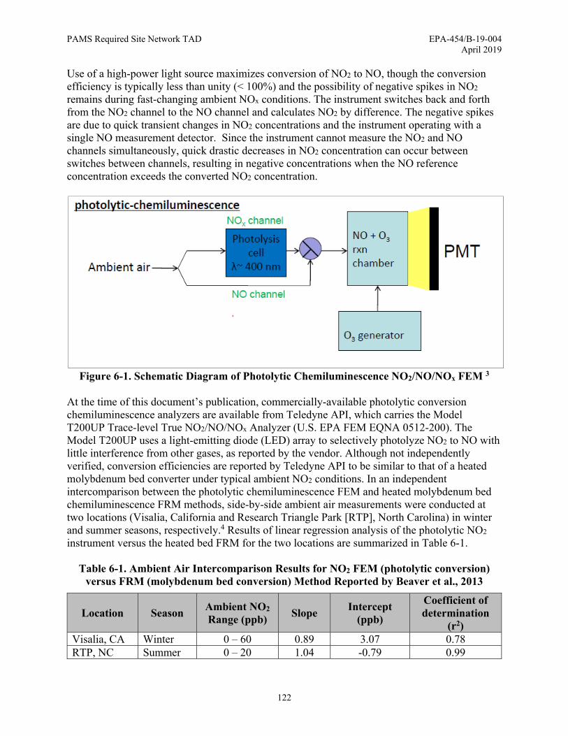
PAMS Required Site Network TAD EPA-454/B-19-004 April 2019
122
Use of a high-power light source maximizes conversion of NO2 to NO, though the conversion efficiency is typically less than unity (< 100%) and the possibility of negative spikes in NO2 remains during fast-changing ambient NOx conditions. The instrument switches back and forth from the NO2 channel to the NO channel and calculates NO2 by difference. The negative spikes are due to quick transient changes in NO2 concentrations and the instrument operating with a single NO measurement detector. Since the instrument cannot measure the NO2 and NO channels simultaneously, quick drastic decreases in NO2 concentration can occur between switches between channels, resulting in negative concentrations when the NO reference concentration exceeds the converted NO2 concentration.
Figure 6-1. Schematic Diagram of Photolytic Chemiluminescence NO2/NO/NOx FEM 3
At the time of this document’s publication, commercially-available photolytic conversion chemiluminescence analyzers are available from Teledyne API, which carries the Model T200UP Trace-level True NO2/NO/NOx Analyzer (U.S. EPA FEM EQNA 0512-200). The Model T200UP uses a light-emitting diode (LED) array to selectively photolyze NO2 to NO with little interference from other gases, as reported by the vendor. Although not independently verified, conversion efficiencies are reported by Teledyne API to be similar to that of a heated molybdenum bed converter under typical ambient NO2 conditions. In an independent intercomparison between the photolytic chemiluminescence FEM and heated molybdenum bed chemiluminescence FRM methods, side-by-side ambient air measurements were conducted at two locations (Visalia, California and Research Triangle Park [RTP], North Carolina) in winter and summer seasons, respectively.4 Results of linear regression analysis of the photolytic NO2 instrument versus the heated bed FRM for the two locations are summarized in Table 6-1.
Table 6-1. Ambient Air Intercomparison Results for NO2 FEM (photolytic conversion) versus FRM (molybdenum bed conversion) Method Reported by Beaver et al., 2013
Location Season Ambient NO2 Range (ppb)
Slope Intercept
(ppb)
Coefficient of determination
(r2) Visalia, CA Winter 0 – 60 0.89 3.07 0.78RTP, NC Summer 0 – 20 1.04 -0.79 0.99
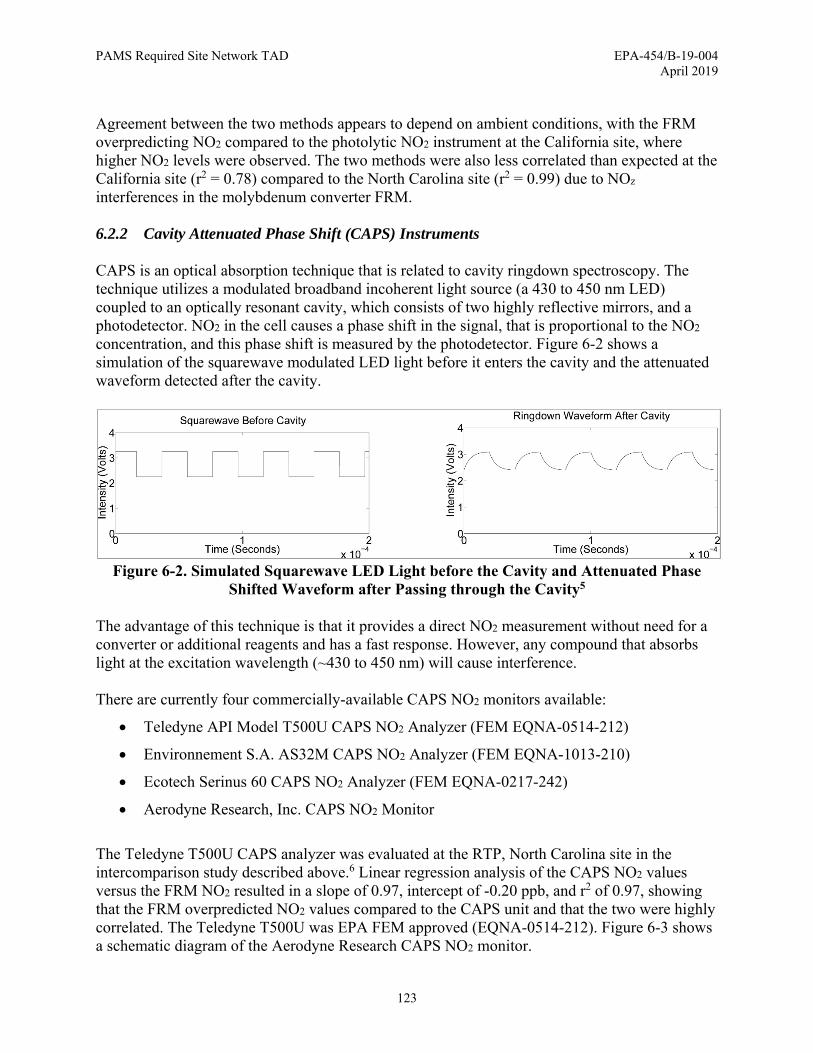
PAMS Required Site Network TAD EPA-454/B-19-004 April 2019
123
Agreement between the two methods appears to depend on ambient conditions, with the FRM overpredicting NO2 compared to the photolytic NO2 instrument at the California site, where higher NO2 levels were observed. The two methods were also less correlated than expected at the California site (r2 = 0.78) compared to the North Carolina site (r2 = 0.99) due to NOz interferences in the molybdenum converter FRM. 6.2.2 Cavity Attenuated Phase Shift (CAPS) Instruments CAPS is an optical absorption technique that is related to cavity ringdown spectroscopy. The technique utilizes a modulated broadband incoherent light source (a 430 to 450 nm LED) coupled to an optically resonant cavity, which consists of two highly reflective mirrors, and a photodetector. NO2 in the cell causes a phase shift in the signal, that is proportional to the NO2 concentration, and this phase shift is measured by the photodetector. Figure 6-2 shows a simulation of the squarewave modulated LED light before it enters the cavity and the attenuated waveform detected after the cavity.
Figure 6-2. Simulated Squarewave LED Light before the Cavity and Attenuated Phase
Shifted Waveform after Passing through the Cavity5 The advantage of this technique is that it provides a direct NO2 measurement without need for a converter or additional reagents and has a fast response. However, any compound that absorbs light at the excitation wavelength (~430 to 450 nm) will cause interference. There are currently four commercially-available CAPS NO2 monitors available:
Teledyne API Model T500U CAPS NO2 Analyzer (FEM EQNA-0514-212)
Environnement S.A. AS32M CAPS NO2 Analyzer (FEM EQNA-1013-210)
Ecotech Serinus 60 CAPS NO2 Analyzer (FEM EQNA-0217-242)
Aerodyne Research, Inc. CAPS NO2 Monitor
The Teledyne T500U CAPS analyzer was evaluated at the RTP, North Carolina site in the intercomparison study described above.6 Linear regression analysis of the CAPS NO2 values versus the FRM NO2 resulted in a slope of 0.97, intercept of -0.20 ppb, and r2 of 0.97, showing that the FRM overpredicted NO2 values compared to the CAPS unit and that the two were highly correlated. The Teledyne T500U was EPA FEM approved (EQNA-0514-212). Figure 6-3 shows a schematic diagram of the Aerodyne Research CAPS NO2 monitor.
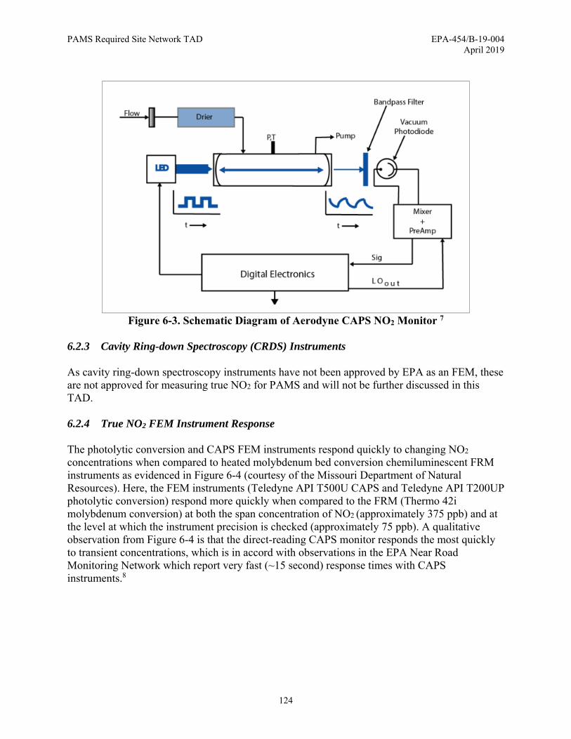
PAMS Required Site Network TAD EPA-454/B-19-004 April 2019
124
Figure 6-3. Schematic Diagram of Aerodyne CAPS NO2 Monitor 7
6.2.3 Cavity Ring-down Spectroscopy (CRDS) Instruments As cavity ring-down spectroscopy instruments have not been approved by EPA as an FEM, these are not approved for measuring true NO2 for PAMS and will not be further discussed in this TAD. 6.2.4 True NO2 FEM Instrument Response The photolytic conversion and CAPS FEM instruments respond quickly to changing NO2 concentrations when compared to heated molybdenum bed conversion chemiluminescent FRM instruments as evidenced in Figure 6-4 (courtesy of the Missouri Department of Natural Resources). Here, the FEM instruments (Teledyne API T500U CAPS and Teledyne API T200UP photolytic conversion) respond more quickly when compared to the FRM (Thermo 42i molybdenum conversion) at both the span concentration of NO2 (approximately 375 ppb) and at the level at which the instrument precision is checked (approximately 75 ppb). A qualitative observation from Figure 6-4 is that the direct-reading CAPS monitor responds the most quickly to transient concentrations, which is in accord with observations in the EPA Near Road Monitoring Network which report very fast (~15 second) response times with CAPS instruments.8

PAMS Required Site Network TAD EPA-454/B-19-004 April 2019
125
Figure 6-4. NO2 FRM and FEM Response Time 8
6.2.5 Minimizing Bias in NO2 Measurements Measurement bias can result from incorrect calibration technique, uncalibrated or poorly calibrated gas metering devices, background due to contaminants in standard gases or diluent gases, poor instrument hygiene, incompatible materials in standard or sampling flow paths, or instrument drift. It is important to minimize the influence of these sources of bias to the extent possible. Standard gases should be sourced from reputable suppliers, and the sourced standards should indicate acceptably low levels of contaminants or interferences and should comply with the EPA Traceability Protocol for Assay and Certification of Gaseous Calibration Standards.9 Several gas suppliers offer such EPA Protocol Gases for which the certified concentrations are traceable to a reference material, such as those prepared and certified by the NIST or the Van Swinden Laboratorium (VSL). COAs for such standards should indicate the traceability to a calibrated instrument and the associated certified standard employed to calibrate the instrument. In general, stock standard gases of NO or NO2 require specially-treated cylinders to ensure the standard gas concentration is stable for the indicated expiration period. For monitoring agencies performing gas phase titration (GPT) of ozone and NO to generate NO2 calibration gas, the levels of residual NO2 in the NO cylinder should not exceed 1% of the NO concentration. Such will be listed on the cylinder COA; however, proper cylinder purging and handling procedures should be practiced to ensure ambient air entrained in the regulator is purged and is not permitted to backflow into the cylinder which can result in the formation of NO2 in the cylinder when oxygen reacts with the NO standard gas. Furthermore, regulators should be purged properly before each

PAMS Required Site Network TAD EPA-454/B-19-004 April 2019
126
use, as practical, to remove contaminants such as water. Refer to the guidance beginning on page 5 of Issue 15 of The QA Eye Newsletter from December 2013, available at the following link:
https://www3.epa.gov/ttnamti1/files/ambient/qa/qanews15.pdf Cylinder regulators, tubing, connecting components, valves, and other portions of the wetted pathway for transferring stock and diluted gas standards and sampled atmosphere should be of compatible materials, namely PTFE or chromatographic-grade stainless steel. Incompatible materials include, but are not limited to: plastic, rubber, brass, and copper. As with the proper purging of cylinder regulators, gas lines should be properly purged to ensure the pathways have been properly passivated prior to utilizing measurements in generating calibration responses. This is typically accomplished by observing instrument response until a stable measurement is achieved. MFCs in dynamic dilution calibrators (DDC) used for gas-phase dilution and GPT should be calibrated at their range of use within the previous 12 months and have the flow calibration verified quarterly. Monitoring agencies should perform maintenance on the zero air generator(s) as indicated by the manufacturer recommendations and prescribed in the appropriate SOP. Instrument maintenance (mirror cleaning, UV lamp replacement, and particulate filter changes) should be conducted per the manufacturer recommendations and per the appropriate SOP. Lastly, the instrument zero drift should be monitored and adjusted per the guidance listed in validation template Appendix D of the EPA QA Handbook, Volume II, January 2017. As of the publication of this TAD, the allowable zero drift was < ± 3.1 ppb NO2 over 24 hours and < ± 5.1 ppb over 14 days. 6.2.6 Generation of NO2 Standards NO2 standards can be prepared using either GPT or dilution of a known concentration of a certified NO2 stock standard gas from a high-pressure cylinder. While both methods are discussed below, monitoring agencies have reported slow instrument responses and a negative bias (refer to Section 6.2.6.2) with dilution of NO2 from a high-pressure cylinder. 6.2.6.1 Gas Phase Titration GPT has been widely employed to generate standard concentrations of NO2 and is described in detail in the EPA Quality Assurance Handbook, Volume II, Part II, Section 2.3.1 (2002). Briefly, generation of NO2 concentrations by GPT is performed by providing a known amount of ozone and providing excess NO. The stoichiometry of the reaction of NO and ozone is such that for every mole of ozone, one mole of NO2 is produced per the following reaction: NO + O3 → NO2 + O2 The NO2 is generated in the mixing area of the DDC and assumes that all ozone is consumed to generate NO2. Advantages of this method of NO2 standards generation are:
The NO reagent is stable in high pressure cylinders

PAMS Required Site Network TAD EPA-454/B-19-004 April 2019
127
NO2 contamination in the NO standards is typically a small, negligible percentage (e.g., < 1%) and is unlikely to increase with appropriate cylinder hygiene
Passivation times of gas supply lines are minimized resulting in fast response of downstream analyzers
The disadvantages to GPT include:
Inability to generate single-digit ppb or lower concentrations as ozone generators are not typically stable at such low concentrations
NO gas cylinders can be easily contaminated
Requires frequent calibration of the DDC ozone generator
6.2.6.2 Dilution of Standard NO2 Gas Stock standard NO2 gas may be sourced from reputable gas providers and the gas diluted with zero air with a DDC to desired concentrations. A small number of monitoring agencies have reported success with directly diluting calibration-level concentrations of NO2 with a DDC from a high pressure cylinder. However, monitoring agencies have generally indicated problems with calibration with such methods. Reports indicate that the calibration appears to be biased low by several percent (approximately 7 to 13%) when compared to a calibration performed with GPT and that stabilization time at each concentration level is extensive, in some instances up to an hour or longer, with the measured concentration gradually increasing to a plateau as illustrated in Figure 6-5 (courtesy Pinellas County Air Quality Division). This method provides the ability to generate low concentration (sub-ppb) standards such as those needed for determining MDLs; however, monitoring agencies should consider the potential bias and extensive stabilization times for routine calibration use.
Figure 6-5. Calibration of CAPS NO2 Analyzer using NO2 Dilution Method 10

PAMS Required Site Network TAD EPA-454/B-19-004 April 2019
128
6.2.7 Calibration of True NO2 Instruments The calibration of the true NO2 instruments is established by introducing zero blanks and span levels of an NO2 standard to the instrument at approximately 80% of the full scale of the selected instrument reporting range. The determined instrument responses are used to set the slope and offset of the calibration. The zero calibration is performed first and the span calibration point follows. The span calibration point should be greater than approximately 80% of the expected measured concentrations. For example, if the full-scale (expected) measurement range is 200 ppb, the span concentration would be approximately 160 ppb. Once the calibration is established, the instrument operator immediately verifies the calibration with a multi-point verification (MPV) consisting of analyzing five concentration levels covering the full-scale range and including a zero (for example, a full-scale range of 0 to 200 ppb, the points could be: 0, 25, 75, 125, 175 ppb). The resulting measured concentrations are fit to a linear regression which will show:
Correlation coefficient, r2 ≥ 0.995
x-intercept within ± 0.2 ppb of origin
each concentration level is within 10% of the nominal concentration
Corrective action should be taken for failures, which may include performing instrument maintenance (cleaning mirrors, replacing particulate filters, etc.) followed by recalibrating the instrument. 6.2.8 True NO2 Sampling True NO2 measurements shall be conducted continuously every day during the PAMS sampling period; data shall be reported as hourly averages in ppb. Sampling hours for which less than 45 minutes of measurement are available are considered to be incomplete, are not valid, and are to be reported to AQS with a null qualifier. For NO2 measurements, the ambient air inlet should be positioned 2 to 15 m above the ground and at least 1 m in horizontal and vertical distance from supporting structures. The distance between the inlet and any surrounding trees shall be at least 10 m, and is recommended to be at least 20 m. 6.2.9 Method Detection Limits for Continuous Gaseous Criteria Pollutant Methods Determination of the MDLs for continuous gaseous monitors, including instruments for true NO2, ozone, and NO/NOy, is performed according to a similar convention. The MDL is determined according to the MUR as described in Section 3.3.5.1, where a series of low concentration standards and blanks is analyzed to establish the instrument variability at low concentration and the average blank background. These aspects are input into the MDL procedure to establish the lowest concentration that is distinguishable from background with 99% confidence. Experience has shown that the manufacturer published MDLs detailed in the FRM/FEM designation for the instruments typically represent an ideal instrument operation and are unrealistically low in practical terms. The monitoring agency should establish an MDL for the instruments initially, preferably prior to PAMS season. EPA has convened an MDL workgroup as part of the PAMS Required Site workgroup to develop guidance for the equipment

PAMS Required Site Network TAD EPA-454/B-19-004 April 2019
129
specifications, standard materials, and procedures for determining MDLs for the various true NO2 FEMs. Note that at the time of this document’s publication, the workgroup was in process and had not published such guidance. A brief general discussion for determining continuous gaseous monitor MDLs follows. Prior to determining the MDL, the instrument is shown to be free of interferences and contamination and an initial calibration is established. Instrument maintenance, such as lamp replacement, mirror cleaning, and particulate filter replacement should be completed prior to beginning the MDL process. The instrument operator conducts the MDL determination by measuring zero air blanks and a low concentration standard. In order to capture an aspect of temporal variability, the measurements for the zero blanks and standards should occur over the course of three different dates, preferably non-consecutive. Once calibrated, the instrument zero drift should not be adjusted throughout the course of the MDL determination. This allows any variability related to the instrument drift to be characterized in the MDL determination. Measurements, activities performed, and equipment used should be documented so that MDL determinations can be reconstructed. An example scenario for determining an MDL with calculations is shown in Section 6.2.9.5. 6.2.9.1 Determining the MDLb Once the instrument is calibrated, the instrument operator introduces zero air to the instrument and measures the zero air matrix as is done for routine zero checks. The instrument operator should review the short-term data (e.g., 5-minute or 1-minute data) to ensure the instrument background is stable and not continuing to decrease. Experienced instrument operators should use their best judgement to determine that the blank reading is stable. The instrument measurements of zero air blank data are recorded for minimally seven discrete 20- to 30-minute periods over the course of minimally three different dates, preferably non-consecutive. The average is computed for each of these seven measurement periods to generate seven concentration values. More than seven blanks can be included in the calculation, and, when included, will typically provide a better approximation of the background contribution. Zero blanks with technical problems (e.g., power surge detector spikes, missing minute data, or ambient air leaks) may be excluded from the subsequent calculations; however, a valid technical reason to exclude data should be documented and justified. The MDLb is calculated as follows:
1. Calculate the average concentration of the zero blank measurement concentrations, b. If xb < 0, let xb = 0.
2. Calculate the standard deviation of the zero blank measurement concentrations, sb.
3. Multiply sb by the one-sided 99th percentile Student’s t value corresponding to the number of blanks analyzed (refer to Table 3-3). Values of t for additional samples (n > 34) may be found in standard statistical tables.

PAMS Required Site Network TAD EPA-454/B-19-004 April 2019
130
4. Calculate MDLb as the sum of b and the product of sb and the associated Student’s t value:
MDLb = b+ sb·t
6.2.9.2 Determining the MDLsp The most difficult aspect of determining the MDLsp portion of the MDL is generating suitable low concentration standards. Modern “trace” level analyzers are capable of detecting single-ppb concentrations of gaseous criteria pollutants, and the ability to generate concentrations in this range is limited by the starting stock gas concentration and the effective DF of the gas calibrator used to generate the standards. In general, generating true NO2 concentrations in the range suitable for determining MDLs (< 1 ppb) is not possible with GPT due to the inability of onboard ozone generators to reliably produce accurate and stable ozone concentrations < 1 ppb. In such cases, it may be more practical to source NO2 from a pressurized cylinder to dilute into the proper range for delivering the standards. As discussed in Section 6.2.6.2, preparation of standard concentrations by dilution of NO2 from a high pressure cylinder can be difficult as it may require extensive times for passivating delivery lines and ensuring a stable instrument response; however, once stabilized, this method of standard gas preparation provides better control of the challenged concentration and the ability to generate low (sub-ppb) concentrations reliably. The first step in determining the MDLsp is selecting a concentration at which to perform the MDLsp procedure. To select a concentration, instrument operators should consider the following, in decreasing order of importance:
1. The concentration at which the instrument response is approximately three- to five-fold the baseline response.
2. Analysis of a suite of zero blanks, such as the measurements recorded determining MDLb - calculate the standard deviation of the measured concentration and multiply by 3.
3. Previously acceptable MDL studies and related experience.
As practical, this selected concentration would be generated to determine the MDLsp. If the standards dilution equipment cannot generate a concentration sufficiently low to achieve that selected, the instrument operator should generate as low as concentration as possible given the system limitations. This may require use of the highest diluent flow possible combined with the lowest flow available on the DDC. Recall that the absolute accuracy of the challenged concentration is not evaluated in the determination and is not as important as the ability to generate a stable concentration. Therefore, operation of the DDC channels outside the typical operating range of 10 to 90% full scale will not impact the MDL determination. Similarly to the MDLb, instrument measurements of the low level concentration standard are recorded for minimally seven discrete 20- to 30-minute measurement periods over the course of minimally three different dates, preferably non-consecutive. The instrument operator should review the short-term data (e.g., 5-minute or 1-minute data) to ensure the instrument reading is stable and not demonstrating an increasing or decreasing trend. Experienced instrument operators should use their best judgement to determine that the reading is stable. The average is computed for each of these seven measurement periods to generate seven concentration values. All

PAMS Required Site Network TAD EPA-454/B-19-004 April 2019
131
appropriate data collected should be included unless a valid technical reason exists to exclude the data. Standard measurement periods with technical problems (e.g., power surge detector spikes, missing minute data, or ambient air leaks) may be excluded; however, a valid technical reason to exclude data should be documented and justified. Calculate the MDLsp as follows:
a. Calculate the standard deviation of the calculated concentrations for the standard measurement periods (ssp).
b. Calculate the MDL for the standard measurement periods (MDLsp) by multiplying ssp by the one-sided 99thth percentile Student’s t value at 99% confidence corresponding to the number of measurement periods analyzed according to Table 3-3. Other values of t for additional samples (n > 34) may be found in standard statistical tables. MDLsp = ssp·t
Compare the resulting calculated MDLsp value to the nominal standard level. The nominal spiked level should be greater than MDLsp and less than 10-fold MDLsp. If this is not the case, the MDLsp process should be repeated with an adjusted spiking concentration, if possible. For MDLsp values greater than the nominal spike level, the MDL spiking level should be adjusted higher by approximately two or three-fold. For nominal spike levels which are greater than the 10-fold the MDLsp, the MDL spiking level should be adjusted lower by approximately two or three-fold. 6.2.9.3 Calculating and Verifying the Instrument MDL Compare MDLsp and MDLb. The higher of the two values is reported as the MDL for the given analyte.
1. If the MDL is determined as the MDLsp, the determined MDL should be verified by:
a. Analyzing one or more standard levels at one- to five-fold of the determined MDL to ensure the determined MDL is reasonable. Recall that at the MDLsp concentration there is a 50% chance that the analyte will not be detected; however, the analyte should be detected at two- to five-fold the determined MDL.
b. Comparing the measured values to reasonable acceptance criteria for the MDL verification. For example, an MDL verification that recovers 2% of the nominal amount is not realistic, nor is one that recovers 300%. Appropriate acceptance limits are to double the acceptance window prescribed by the method for the given analyte. For example, for ozone measurements, the bias specification is ±7, therefore 14% may be achievable. Note that agencies may develop alternate acceptance criteria through control charts or other similar tools. For methods with a significant background contamination, blank subtraction may be necessary to evaluate the recovery of the MDL verification standard.
c. Examining the MDL procedure for reasonableness if the verification sample is outside of the laboratory-defined acceptance criteria. Such an examination might include investigating the S:N ratio of the analyte response in the standard data and relying on instrument operator experience and expertise to evaluate the MDL

PAMS Required Site Network TAD EPA-454/B-19-004 April 2019
132
procedure and select a different spiking level. The MDL study should then be repeated with a different spiking level, if possible.
6.2.9.4 Ongoing Determination of the Instrument MDL Once the MDL has been initially established, the MDL should be re-determined when changes to the instrument would reasonably expect to affect the sensitivity (such may include replacing a detector lamp, detector, and/or flow cell mirrors, for example). MDL standards could be measured periodically to prepare a dataset for calculating MDLsp (as in Section 6.2.9.2) and the ongoing collection of routine zero blank data would provide a population of blanks to calculate MDLb (as in Section 6.2.9.1). If changes have not been made to the instrument that affect sensitivity, the MDL should be updated annually by including these ongoing collected zero blank and low level standard hourly data. Calculate the MDLb and MDLsp as described in Sections 6.2.9.2 and 6.2.9.3 and update the method MDL for the monitor. 6.2.9.5 Example MDL Calculation for Continuous Gaseous Criteria Pollutant Monitors A site is determining the MDL for a brand new true NO2 instrument. The instrument is powered on and conditioned per the manufacturer instructions and then is calibrated per the monitoring agency SOP. Over the course of a week, the instrument is challenged with zero air for several 20- to 30-minute periods every other day and the values combined to generate the MDLb. The monitoring agency also uses blank data to determine an approximate spiking level based on the variability of the zero blanks as in Section 6.2.9.2. The site determines the approximate spiking concentration by calculating the standard deviation of the suite of zero blanks and multiplying this by three. This value is approximately 0.33 ppb and is rounded up to 0.5 ppb to achieve a better instrument signal based on recording some measurements in the zero blanks at approximately 0.4 ppb. The following week, the instrument is challenged with an NO2 standard every other day by diluting a cylinder of NO2 to 0.5 ppb with zero air with a DDC. Once the true NO2 instrument response shows a stable response each day, the averages for each measurement period are computed. The average ( ) and standard deviation (s) of measured average true NO2 concentrations are determined for both the zero blanks and known standard analyses of 0.5 ppb. Refer to the collected data in Table 6-2. To calculate the MDLb, the standard deviation of the zero blank measurements (sb) is multiplied by the associated student’s T for the 27 aliquots (degrees of freedom = 26) and this product is added to the average blank value, b: MDLb = 0.110 ppb · 2.479 + 0.248 ppb
= 0.521 ppb

PAMS Required Site Network TAD EPA-454/B-19-004 April 2019
133
Table 6-2. Example True NO2 MDL Determination
Zero Blank sample date and start time
Zero Blank measurement period
average (ppb)
Standard Analysis sample date and start time
Standard Analysis measurement period
average (ppb)
3/8/18 9:00 0.247 3/15/18 10:00 0.552 3/8/18 10:00 0.323 3/15/18 11:00 0.504 3/8/18 11:00 0.178 3/15/18 12:00 0.612 3/8/18 12:00 0.371 3/15/18 13:00 0.688 3/8/18 13:00 0.098 3/15/18 14:00 0.512 3/8/18 14:00 0.212 3/15/18 15:00 0.663 3/8/18 15:00 0.090 3/15/18 16:00 0.443 3/8/18 16:00 0.112 3/15/18 17:00 0.529 3/8/18 17:00 0.265 3/15/18 18:00 0.422 3/10/18 9:00 0.400 3/17/18 10:00 0.602
3/10/18 10:00 0.146 3/17/18 11:00 0.555 3/10/18 11:00 0.220 3/17/18 12:00 0.514 3/10/18 12:00 0.441 3/17/18 13:00 0.633 3/10/18 13:00 0.356 3/17/18 14:00 0.642 3/10/18 14:00 0.214 3/17/18 15:00 0.611 3/10/18 15:00 0.141 3/17/18 16:00 0.472 3/10/18 16:00 0.443 3/17/18 17:00 0.522 3/10/18 17:00 0.312 3/17/18 18:00 0.599 3/12/18 9:00 0.167 3/19/18 10:00 0.623
3/12/18 10:00 0.224 3/19/18 11:00 0.492 3/12/18 11:00 0.163 3/19/18 12:00 0.466 3/12/18 12:00 0.089 3/19/18 13:00 0.616 3/12/18 13:00 0.311 3/19/18 14:00 0.546 3/12/18 14:00 0.254 3/19/18 15:00 0.612 3/12/18 15:00 0.443 3/19/18 16:00 0.678 3/12/18 16:00 0.267 3/19/18 17:00 0.445 3/12/18 17:00 0.222 3/19/18 18:00 0.687
total zero blanks (n) 27 total standard analyses (n) 27 degrees of freedom (n-1) 26 degrees of freedom (n-1) 26 student's T for n-1 = 26 2.479 student's T for n-1 = 26 2.479 b (ppb) 0.248 sp (ppb) 0.564
sb 0.110 ssp (ppb) 0.080 student's T 2.479 student's T 2.479 MDLb (ppb) 0.521 MDLsp (ppb) 0.197 3· sb 0.330
To calculate the MDLsp, the standard deviation of the standard analyses (ssp) is multiplied by the associated student’s T for the 27 aliquots (degrees of freedom = 26). MDLsp = 0.080 ppb · 2.479
= 0.197 ppb
The MDLsp is subsequently verified to be less than the nominal standard level, and the nominal standard level is confirmed to be less than 10-fold the MDLsp: MDLsp < nominal standard level < 10-fold MDLsp 0.197 ppb < 0.5 ppb < 1.97 ppb

PAMS Required Site Network TAD EPA-454/B-19-004 April 2019
134
The MDLsp and MDLb are compared to determine which is greater, and the greater of the two values is reported as the monitor MDL. 0.521 ppb > 0.197 ppb The monitor reported MDL is 0.521 ppb. 6.2.10 True NO2 Quality Control 40 CFR Part 58, Appendix A provides details about the number of QC samples that will be implemented for FRMs and FEMs. The QC parameters and acceptance criteria are shown in Table 6-3. For NO2, QC samples should include the following:
Zero point checks – Bi-weekly zero point checks are conducted analyzing gas provided by zero air generators. The NO2 analyzer will operate in its normal sampling mode during the QC check and the test atmosphere will pass through all filters, scrubbers, conditioners and other components used during normal ambient sampling and as much of the ambient air inlet system as is practicable. The QC check is to be conducted before any calibration or adjustment is made to the monitor. The zero will be ≤ 0.2 ppb or MDL, whichever is lower.
QC checks – A one-point QC check for NO2 will be performed at least once every 2 weeks on each automated monitor used to measure NO2; however, more frequent checking is strongly encouraged. The QC check is made by challenging the monitor with a standard gas of known concentration selected to represent the approximate mean or median concentrations at the site. If the mean or median concentrations are below the MDL of the instrument, the monitoring agency can select the lowest concentration in the prescribed range that can be practically measured. If the mean or median concentrations are above the prescribed range the agency can select the highest concentration in the prescribed range. An additional QC check point is encouraged for those organizations that may have occasional high values or would like to confirm the monitor linearity at the higher end of the operational range or around NAAQS concentrations. The NO2 analyzer will operate in its normal sampling mode during the QC check and the test atmosphere is to pass through all filters, scrubbers, conditioners and other components used during normal ambient sampling and as much of the ambient air inlet system as is practicable. The QC span check is conducted before any calibration or adjustment is made to the monitor. These one-point QC span checks should be reported to AQS. The percent differences between these concentrations are used to assess the precision and bias of the monitoring data. Measured values will be within ± 10% of the nominal concentration.
Span Point – A bi-weekly span point is performed at 80 to 90% of the analyzer full scale. The span check concentration should be above 99% of the routine data over a 3-year period. Measured values will be within ± 10% of the nominal concentration.
Precision Point – A bi-weekly standard point in the lower third of the full-scale range. Measured values will be within ± 10% of the nominal concentration.

PAMS Required Site Network TAD EPA-454/B-19-004 April 2019
135
Table 6-3. Quality Control Parameters and Acceptance Criteria for True NO2
QC Parameter Description Required Frequency
Acceptance Criteria Suggested Corrective Action
Initial calibration (ICAL)
Set ZERO and SPAN levels on the true NO2 analyzer using zero air and an NO2 standard at 80% of the full-scale measurement (e.g., 0 and 160 ppb NO2 for a full-scale range of 0 to 200 ppb)
Initially before the beginning of PAMS season, following maintenance to the instrument expected to alter the instrument response, following failing SPAN checks, and at the end of PAMS season
None. Verified by MPV.
Repeat calibration. It may be necessary to investigate for system contamination or interferences resulting in suppression or enhancement.
Multipoint Verification (MPV)
Verification performed by analyzing five concentration points including a zero and covering the calibration range. (e.g., 0, 25, 75, 125, and 175 ppb)
Immediately following establishing a new calibration
For linear regression, will show r2 of ≥ 0.995 and have an x-intercept within ± 0.2 ppb NO2 of the origin. Each standard level evaluated against the calibration curve will be within 10% of the nominal concentration.
Repeat verification. It may be necessary to investigate for system contamination or interferences resulting in suppression or enhancement of analytes. Recalibration may be necessary.
Zero/Span Verification
Analysis of zero air and mid-level NO2 standard to monitor for drift in zero and span levels
Optional, recommended daily during nighttime hours
Zero level will be less than 0.2 ppb or analyzer MDL, whichever is lower. Span level will be within 10% of the nominal concentration.
Repeat zero and span checks. Investigate system for contamination. Qualify data since the last passing zero/span check. May be necessary to repeat ICAL and MPV.
Zero/Span/Precision Verification
Verification performed by analyzing three points including a zero and two standard concentration levels. (e.g., 0, 170, 50 ppb)
Biweekly – The SPAN check is reported to AQS
Zero level will be less than 0.2 ppb or analyzer MDL, whichever is lower. Span level will be within 10% of the nominal concentration.
Repeat Zero/Span/Precision Verification. Investigate system for contamination. Qualify data since the last passing zero/span check. May be necessary to repeat ICAL and MPV.
6.3 NOy A standard reference method for total reactive gaseous nitrogen (NOy) has not been designated. However, an instrument design modification of the NOx heated bed chemiluminescence approach by moving the converter to the sample inlet avoids line loss of adsorbent NOy species, such as HNO3, is in wide use (Figure 6-6). Measurement of NOy is described in detail in the EPA Precursor Gas TAD, Section 4.1 NOy measurements conducted for NCore are acceptable for the

PAMS Required Site Network TAD EPA-454/B-19-004 April 2019
136
PAMS network. Following is a summary of commercially-available NOy measurement technologies.
Figure 6-6. Summary of Commercially-Available NOy Analyzers 11
6.4 References 1. Technical Assistance Document (TAD) For Precursor Gas Measurements in the NCore
Multi-Pollutant Monitoring Network, Version 4, EPA-454/R-05-003, September 2005. Available at (accessible March 2018): https://www3.epa.gov/ttnamti1/ncore/guidance/tadversion4.pdf
2. Quality Assurance Handbook for Air Pollution Measurement Systems. Volume II – Ambient Air Quality Monitoring Program, EPA-454/B-08-002, U. S. Environmental Protection Agency, January 2017.
3. Beaver, Long, and Kronmiller “Characterization and Development of Measurement Methods for Ambient Nitrogen Dioxide (NO2),” May 16, 2012
4. Beaver et al., Direct and Indirect Methods for the Measurement of Ambient Nitrogen Dioxide. Extended Abstract 57, Conference, 2013.
5. T. K. Boyson, T. G. Spence, M. E. Calzada, and C. C. Harb, "Frequency domain analysis for laser-locked cavity ringdown spectroscopy," Opt. Express 19, 8092-8101 (2011) [FIGURE C]

PAMS Required Site Network TAD EPA-454/B-19-004 April 2019
137
6. Beaver, M., K. Kronmiller, R. Duvall, S. Kaushik, T. Morphy, P. King, and R. Long. Direct and Indirect Methods for the Measurement of Ambient Nitrogen Dioxide. Presented at AWMA Measurement Technologies meeting, Sacramento, CA, November 19 - 21, 2013.
7. Aerodyne Research, Inc. CAPS NO2 Monitor brochure, accessed February 2018. http://www.aerodyne.com/sites/default/files/CAPS%20NO2%202015.pdf
8. Kuebler, Dustin, and Gaddie, Satchel. NO2 Measurement: A Comparison of Direct vs. Traditional Methods at a Near-Roadway Site. Missouri Dept of Natural Resources. Available at (accessed March 2018): https://dnr.mo.gov/env/apcp/docs/NO2%20Measurement%20--%20A%20Comparison%20of%20Direct%20vs.%20Traditional%20Methods%20at%20a%20Near-roadway%20Site.pdf
9. U.S. EPA EPA Traceability Protocol for Assay and Certification of Gaseous Calibration Standards. EPA/600/R-12/531. May 2012. Available at: https://cfpub.epa.gov/si/si_public_file_download.cfm?p_download_id=522029&Lab=NRMRL Accessed February 2019.
10. Taylor, Vicki. API NO2 CAPS Performance Review. Presented at the 2017 EPA Region 4 Ambient Air Monitoring Conference.
11. Russell Long. Overview of ORD NO2, NOx and NOy Measurement Research. Presented at NAAMC August 8-11, 2016.

PAMS Required Site Network TAD EPA-454/B-19-004 April 2019
138
7.0 OZONE EPA revised the primary and secondary O3 standard NAAQS to 0.070 ppm in 2015. Ambient air ozone monitoring has been a component of the State and Local Ambient Monitoring Stations since the 1970s. Ozone monitoring will take place at PAMS sites using automated FRMs or FEMs, as established in 40 CFR Appendix C to Part 58, Ambient Air Quality Monitoring Methodology. Ozone measurements will be conducted continuously on a daily basis during the PAMS monitoring period and measurements reported as hourly averages. Production of tropospheric ozone, the concentration of which is regulated under the CAA, occurs through complex reaction chemistry involving NOx and VOCs, as introduced previously in the discussion of NOx, above. The atmospheric processes involved in ozone photochemistry are complex; a simplified representation is shown in Figure 7-1. Generally, high ozone concentrations are most likely to reach unhealthy levels and exceed EPA’s ozone standards in urban areas on warm, sunny summer days. However, the lifetime of ozone in the troposphere is sufficient to cause elevated ozone concentrations in downwind rural areas. Ozone reduction programs generally target emission control strategies for VOCs and/or NOx – as ozone precursors. Since ozone production rates are not linear with respect to VOC and NOx concentrations, atmospheric modeling of ozone photochemistry and meteorology is needed to design effective control strategies. Concentration measurements from the PAMS program assists modelers in the evaluation of the accuracy of these models. Measurement of ozone is required at NCore sites, therefore the policies, procedures, and requirements for ozone measurement will be those as described within the 40 CFR Part 58 Appendix C, NCore Precursor Gas Measurements TAD,1 and in the EPA QA Handbook Volume II.2

PAMS Required Site Network TAD EPA-454/B-19-004 April 2019
139
Figure 7-1. Simplified Representation of Tropospheric Ozone Chemistry Reactions and
Processes 3 7.1 References 1. Technical Assistance Document (TAD) For Precursor Gas Measurements in the NCore
Multi-Pollutant Monitoring Network, Version 4, EPA-454/R-05-003, September 2005. Available at (accessible March 2018): https://www3.epa.gov/ttnamti1/ncore/guidance/tadversion4.pdf
2. Quality Assurance Handbook for Air Pollution Measurement Systems. Volume II – Ambient Air Quality Monitoring Program, EPA-454/B-08-002, U. S. Environmental Protection Agency, January 2017.
3. Sumner, A.L., The role of formaldehyde in tropospheric ozone chemistry, Ph.D. Thesis, Purdue Univ., West Lafayette, IN, 2001.

PAMS Required Site Network TAD EPA-454/B-19-004 April 2019
140
8.0 METEOROLOGY Information and guidance for meteorological measurements are provided in detail in the Quality Assurance Handbook for Air Pollution Measurement Systems, Volume IV - Meteorological Measurements. EPA-454/B-08-002.1 The following summarizes the guidance presented in the Handbook. However, it is recommended that monitoring personnel also read the Handbook for a more complete discussion of these measurements. MLH measurements using ceilometers are not covered in the current version of the EPA QA Handbook, and are consequently discussed in more detail in Section 8.8. The data quality indicators and associated measurement quality objectives for each of the meteorological measurements are presented in Sections 3.2 and 3.3 and in Table 3-1. A summary of meteorology quality control checks is shown in Table 8-1. 8.1 Wind Speed and Wind Direction Wind speed and direction measurements are essential to the evaluation of transport and dispersion processes of all atmospheric pollutants. Wind speed is typically measured with a cup or propeller anemometer; wind direction is typically measured with a wind vane. The use of sonic anemometers has also become more prevalent in recent years. The standard height for surface layer wind measurements is 10 m AGL.1,3,4 The location of the site for the wind measurements should ensure that the horizontal distance to obstructions (e.g., buildings, trees) is at least 10 times the height of the obstruction.1,4 An obstruction may be man-made (e.g., a building) or natural (a tree). A wind instrument should be securely mounted on a mast that will not twist, rotate, or sway. Roof mounting is not recommended and should only be resorted to when absolutely necessary. If a wind instrument must be mounted on the roof of a building, it should be mounted high enough to be out of the wake of an obstruction. Sensor height and its height above the obstructions, as well as the character of nearby obstructions, is to be documented in site planning documentation. An open lattice tower is the recommended structure for monitoring of meteorological measurements at the 10-m level. In the case of wind measurements, certain precautions are necessary to ensure that the measurements are not significantly affected by turbulence in the immediate wake of the meteorological tower. To avoid such tower effects, the wind sensor should be mounted on a mast a distance at least one tower width above the top of the tower, or if the tower is higher than 10 m, on a boom projecting horizontally from the tower. In the latter case, the boom should extend a distance at least twice the diameter/diagonal of the tower from the nearest point on the tower. The boom should project into the direction which provides the least distortion for the most important wind direction (i.e., into the prevailing wind). There are several types of open lattice towers: fixed, tilt-over, and telescopic. A fixed tower is usually assembled as a one-piece structure from several smaller sections. This type of tower must be sturdy enough so that it can be climbed safely to install and service the instruments. Tilt-over towers are also one-piece structures, but are hinged at ground level. This type of tower has the advantage of allowing the instruments to be serviced at the ground. Telescopic 10-m towers are

PAMS Required Site Network TAD EPA-454/B-19-004 April 2019
141
usually composed of three sections, each approximately 4 m in length. The top section is the smallest in diameter and fits inside the middle section which, in turn, fits inside the base section. The tower can be extended to a height of 10 m by use of a hand crank located at the lowest section. The top of the tower can be lowered to a height of about 4 m providing easy access to the wind sensors. Telescopic and tilt-over towers are not generally recommended for heights above 10 m. Regardless of which type of tower is used, the structure should be sufficiently rigid and properly guyed to ensure that the instruments maintain a fixed orientation at all times. Instrumentation for monitoring wind speed and direction should never be mounted on or near solid structures such as buildings, stacks, water storage tanks, cooling towers, etc., because such structures create significant distortions in the flow field. A sensor with a high accuracy at low wind speeds and a low starting threshold is recommended for PAMS applications. Lightweight materials (e.g., molded plastic or polystyrene foam) should be employed for cups and propeller blades to achieve a starting threshold (lowest speed at which a rotating anemometer starts and continues to turn and produce a measurable signal when mounted in its normal position) of < 0.5 m/s. Wind vanes or tail fins should also be constructed from lightweight materials. The starting threshold (lowest speed at which a vane will turn to within 5º of the true wind direction from an initial displacement of 10º) should be < 0.5 m/s. Overshoot must be < 25% and the damping ratio should lie between 0.4 and 0.7. Wind speed measurements should be accurate to within ±0.2 m/s or ±5%, whichever is greater. Wind direction measurements should be accurate to within ±5º including the combined error in the system from the alignment with true north and the error inherent in the instrument. Alignment with true north should be ≤ 1° and instrumental error should be ≤ 3° to ensure the ±5° tolerance threshold is met. 8.2 Temperature Temperature affects photochemical reaction rates and, consequently, is an essential measurement for PAMS applications. Sensors used for monitoring ambient temperature include wire bobbins, thermocouples, and thermistors. Platinum resistance temperature detectors are among the more popular sensors used in ambient monitoring; these sensors provide accurate measurements and maintain a stable calibration over a wide temperature range. The standard height for surface layer ambient temperature measurements is 2 m AGL. Higher mounting is permitted; if a tower is used, the temperature sensor should be mounted on a boom which extends at least one tower width/diameter from the tower. The measurement should be made over a uniform plot of open, level ground at least 9 m in diameter centered on the sensor. The surface should be covered with non-irrigated or un-watered short grass or, in areas which lack a vegetation cover, natural earth. Concrete, asphalt, and oil-soaked surfaces and other similar surfaces should be avoided to the extent possible. The temperature sensor should be at least 30 m horizontally from any such paved area. If these siting criteria (open ground and distance from paved surfaces) cannot be achieved, it should be identified in site characterization documentation. Other areas to avoid include extraneous energy sources (subway entrances, rooftops, electrical transmission equipment), large industrial heat sources, roof tops, steep slopes, hollows, high vegetation, swamps, snow drifts, standing water, tunnels, drainage culverts, and air

PAMS Required Site Network TAD EPA-454/B-19-004 April 2019
142
exhausts. The distance to obstructions for accurate temperature measurements should be at least four times the obstruction height.7 Temperature measurements should be accurate to ±0.5ºC over a range of -30 to +50ºC with a resolution of 0.1ºC. The thermal time constant (the time it takes the temperature sensor to reach 63.2% of the total difference between its initial and final temperature) should be 60 seconds. Solar heating is usually the greatest source of error and, consequently, adequate shielding is needed to provide a representative ambient air temperature measurement. Ideally, the radiation shield should block the sensor from view of the sun, sky, ground, and surrounding objects. The shield should reflect all incident radiation and not reradiate any of that energy towards the sensor. The best type of shield is one which provides forced aspiration at a rate of at least 3 m/s over a radiation range of -100 to +1100 W/m2. Errors in temperature should not exceed ±0.25 ºC when a sensor is placed inside a forced aspiration radiation shield. The sensor must also be protected from precipitation and condensation, otherwise evaporative effects and other forms of radiational heating or cooling will lead to a depressed temperature measurement (i.e., wet bulb temperature). Temperatures may be reported to AQS in ºF or ºC; °C is the standard default temperature unit for AQS. 8.3 Relative Humidity Measurements of atmospheric humidity are essential to understanding chemical reactions involving ozone precursors and water vapor. Measures of atmospheric humidity include vapor pressure, dew point temperature, specific humidity, absolute humidity, and RH. For the PAMS program, RH will be reported. The methods described here to measure the water vapor content of the atmosphere require measuring the ambient temperature and require similarly protecting the measuring probe from temperature influences as ambient temperature monitoring equipment. To protect from such influences, probes are typically installed within naturally or mechanically aspirated shields. Electrical hygrometers are commonly available for measuring RH and are excellent alternatives to chilled-mirror, wet-bulb thermometer, and wire-wound salt-coated bobbin sensors used historically. Modern electrical hygrometers operate by measuring the changes in voltage output of thin hygroscopic films that react to the presence of moisture by changing resistance and capacitance. The moisture changes are correlated with corresponding temperature measurements to determine the RH. The standard height for humidity measurement installation is 2 m AGL. The humidity sensor should be installed using the same siting criteria as used for temperature, noting that nearby standing water should be avoided. If possible, the humidity sensor should be housed in the same aspirated radiation shield as the temperature sensor. The humidity sensor should be protected from contaminants such as salt, hydrocarbons, and particulates. The best protection is the use of a porous membrane filter which allows the passage of ambient air and water vapor while keeping out particulate matter. Measurements should be accurate to ±5% as expressed as RH over a range of 10 to 100% RH.

PAMS Required Site Network TAD EPA-454/B-19-004 April 2019
143
8.4 Solar Radiation Solar radiation refers to the electromagnetic energy in the solar spectrum (0.10 to 4.0 µm wavelength). The solar spectrum is commonly subdivided as ultraviolet (0.10 to 0.40 µm), visible light (0.40 to 0.73 µm), and near-infrared (0.73 to 4.0 µm) radiation. About 97% of the solar radiation reaching the earth’s outer atmosphere lies between 0.29 and 3.0 µm.3 A portion of this energy penetrates through the atmosphere and is either absorbed or reflected at the earth's surface. The remaining radiation is scattered and/or absorbed in the atmosphere before reaching the surface. Solar radiation measurements are used in heat flux calculations, for estimating atmospheric stability, and in modeling photochemical reactions. Energy fluxes in the solar radiation spectrum are measured using a pyranometer. These instruments are configured to measure what is referred to as global solar radiation (i.e., direct plus diffuse [scattered] solar radiation). The sensing element of a typical pyranometer is protected by a clear glass dome to prevent entry of energy (wavelengths) outside the solar spectrum (i.e., long-wave radiation). These glass domes are transparent to wavelengths in the range of 0.28 to 2.8 µm. Solar radiation measurements should be taken in a location with an unrestricted view of the sky in all directions. In general, locations should be avoided where there are obstructions that could cast a shadow or reflect light on the sensor; light colored walls or artificial sources of radiation should be avoided. The horizon as viewed from the pyranometer should not exceed 5 degrees. Sensor height is not critical for pyranometers; consequently, tall platforms or roof tops are typical locations. Regardless of where the pyranometer is sited, it is important to ensure that the instrument is maintained level and that the glass dome is cleaned as necessary. To facilitate leveling, pyranometers should be equipped with an attached circular spirit level. Instrument manufacturer’s specifications should match the requirements of the World Meteorological Organization3 for either a secondary standard or first class pyranometer, in order to meet the performance specifications in Table 3-1. 8.5 Ultraviolet Radiation UV radiation can be divided into three sub-ranges: UV-A (0.315 to 0.400 µm), UV-B (0.280 to 0.315 µm), and UV-C (0.100 to 0.280 µm). Due to absorption by stratospheric ozone, the UV radiation reaching the surface of the earth consists primarily of wavelengths longer than 0.28 µm (UV-A and UV-B ranges). The most important photochemically active chemical species at these wavelengths are ozone, NO2, and formaldehyde; the latter two chemical species are important in the formation of ozone. Pyranometers with a spectral response covering both the UV-A and UV-B (0.280 to 0.400 m) ranges, commonly referred to as “total ultraviolet” or “broadband” radiometers, are recommended for PAMS applications. These instruments provide a relatively constant response covering the UV-A and UV-B ranges and are more suitable for measuring total UV radiation than employing multiple sensors each covering only a portion of the UV spectrum. Users are discouraged from monitoring UV radiation with two separate instruments each uniquely measuring one UV spectral range (e.g., one UV-A instrument and one UV-B

PAMS Required Site Network TAD EPA-454/B-19-004 April 2019
144
instrument), as the typical overlap in response is small and exhibits a depression in the spectral response resulting in under-reporting the total UV. Guidelines for instrument siting of UV radiation sensors are identical to those for solar radiation measurements, above. 8.6 Barometric Pressure Barometric pressure (station pressure) is used in the calculation of fundamental thermodynamic quantities (e.g., air density). The type of sensor used to measure pressure is called a pressure transducer for which there are numerous commercially-available instruments that meet the specifications in Table 3-1. Ideally, the pressure sensor should be located in a ventilated shelter about 2 m AGL. If the pressure sensor is placed indoors, accommodations should be made to vent the pressure port to the outside environment. One end of a tube should be attached to the sensor's pressure port and the other end vented to the outside of the shelter so that pressurization due to the air conditioning or heating system is avoided. The wind can often cause dynamical changes of pressure in a room where a sensor is placed. These fluctuations may be on the order of 2 to 3 hPa when strong or gusty winds prevail. The height of the station above mean sea level and the height of the pressure sensor AGL should be documented. 8.7 Precipitation Precipitation should be measured with a recording precipitation gauge such as a tipping bucket or weighing bucket. Precipitation gauges that operate using acoustic methods typically do not comply with the performance requirements in Table 3-1 and are difficult or impossible to independently audit in the field. The precipitation gauge should be located on level ground in an open area. Obstructions should not be closer than two to four times their height from the instrument. The area around the precipitation gauge should be covered with natural vegetation. The mouth of the gauge should be level and should be as low as possible while still precluding in-splashing from the ground (30 cm AGL is the recommended minimum height). For ease in user access, the gauge should not be mounted higher than 2 m AGL. A wind shield/wind screen (such as an Alter-type wind shield consisting of a ring with approximately 32 free-swinging separate metal leaves) should be employed to minimize the effects of high wind speeds. 8.8 Mixing Layer Height 8.8.1 Definition and Measurement of Mixing Layer Height The planetary boundary layer (PBL), or atmospheric boundary layer, is the lowest part of the Earth's atmosphere. It is directly influenced by its contact with the Earth’s surface. The PBL responds to heat transfer, pollutant emission, and other surface forcings in a timescale of an hour or less.

PAMS Required Site Network TAD EPA-454/B-19-004 April 2019
145
The depth of the PBL depends on the location, season, time of day, and weather. Typically, this boundary layer extends 50 to 3000 m from the Earth's surface. Fog, haze, mist, and air pollution are typical phenomena in the PBL. The PBL contains several layer types:
Convective boundary layer: Layer of air in which particles mix well due to mechanical and thermal forces.
Nocturnal boundary layer: Stable layer of air that forms around sunset. Its top is often marked by a temperature inversion. The layer usually dissolves by convection in the morning hours, but it can also stay during daytime when solar heating is not sufficient to disperse the nocturnal boundary layer.
Residual layer: Layer of air containing the particles left from the previous convective boundary layer after sunset and before the onset of convection the following morning or from long-range transport by winds.
Surface layer: Layer of air that is situated closest to the ground. Its thickness is typically 50 to 100 m, about 10% of the boundary layer height. This is the layer with the greatest wind shear.
There are a variety of different definitions that describe the mixing layer of the atmosphere. The goal for the PAMS measurements is to collect a consistent data set of hourly values describing the mixing height in the lowest atmospheric boundary layer. For the purposes of the intended PAMS measurements, the mixing height is the layer of air adjacent to the ground in which any pollutant or particle released into it will be mixed vertically. If there are multiple layers identified, then the mixing height is the lowest of those layers. The MLH is the height of the layer adjacent to the ground over which pollutants or any constituents emitted within this layer or entrained into it become vertically dispersed by convection or mechanical turbulence. During the day, diurnal variation has the following effects on the planetary boundary layer (see Figure 8-1):
The turbulence in the air is driven by solar radiation and radiative cooling, both of which occur simultaneously. At night, the radiative cooling of the surface controls the boundary layer, creating the nocturnal layer. The nocturnal layer blocks the interference between the surface layer and the residual layer. Before sunrise, the nocturnal boundary layer height is the mixing height as depicted in Figure 8-1.
After sunrise the solar radiation warming the ground destabilizes the surface layer, leading to thermals of warm air that rise upwards initiating the convective mixing process. The thermals continue to rise until their temperature has dropped to the same temperature as the surrounding air. At the same time thermals of cool air sink down from the top of the clouds. The resulting vertical turbulence transport mixes temperature, moisture, and particles uniformly within this convective boundary layer. The convective

PAMS Required Site Network TAD EPA-454/B-19-004 April 2019
146
boundary layer reaches its maximum mixing height in the late afternoon. During daylight hours the convective boundary layer height is the mixing height.
When the convective boundary layer reaches the level of the residual boundary layer, both layers merge together. This is an important process for air pollution transportation in time and space, with this horizontal dispersion and transport of pollutants and particles having a strong influence on the air quality.
When the sun sets, radiative cooling of the ground results in the collapse of the convective boundary layer. Driven by the radiative cooling process, a new nocturnal boundary layer is formed which is again replaced with a new convective boundary layer during the next day.
The entrainment zone is the interface or boundary between the convective boundary layer and free atmosphere.
Figure 8-1. Diurnal Variation of the Planetary Boundary Layer Structure 8
8.8.2 Ceilometer Theory of Operation Ground-based remote sensors such as a ceilometer are effective tools for acquiring upper-air information and have played an increasingly important role in atmospheric boundary layer studies. EPA has demonstrated successful accession of mixing layer height data with the Vaisala Ceilometer CL51. A ceilometer (Figure 8-2) employs pulsed diode laser Light Detection and Ranging technology, where short, powerful laser pulses are sent out in a vertical or near-vertical direction. The reflection of light, backscatter, caused by haze, fog, mist, virga, precipitation, and clouds, is measured as the laser pulses traverse the sky. The resulting

PAMS Required Site Network TAD EPA-454/B-19-004 April 2019
147
backscatter intensity profile, that is, the signal strength versus the height, is stored and processed, and the mixing height is measured using the characteristics of the backscattered profile. The time delay between the launch of the laser pulse and the detection of the backscatter signal provides the measure of the layer heights. The operating principle of a ceilometer is based on the measurement of the time needed for a short pulse of light to traverse the atmosphere from the transmitter emitted from the ceilometer to the top of the backscattering layer and back to the receiver of the ceilometer. The general expression connecting time delay (t) and backscattering height (h) is:
h = ct/2 where c is the speed of light (c = 2.99 × 10⁸ m/s)
A reflection from 25,000 feet can be seen by the receiver after t = 50.9 μs
Figure 8-2. Vaisala CL51 Ceilometer
Using this relationship between time and distance, a vertical backscatter profile is created (see Figure 8-3). The backscatter signal is typically stronger in the planetary boundary layer where particle concentration is higher, but weaker in the free atmosphere where the atmosphere typically has fewer particles.

PAMS Required Site Network TAD EPA-454/B-19-004 April 2019
148
Figure 8-3. Example Vertical Backscatter Profile
8.8.3 Ceilometer Siting and Installation The ceilometer measurements are intended for more macro-scale application than are the surface meteorological measurements. Consequently, the location of the ceilometer site need not be associated with any particular PAMS surface site. Factors that should be considered in selecting a site for the upper-air monitoring include whether the upper-air measurements for the proposed location are likely to provide the necessary data to characterize the meteorological conditions associated with high ozone concentrations, and the extent to which data for the proposed location may augment an existing upper-air network. The ceilometer should be securely installed on a stable level surface such as a concrete pad or wooden platform suitably located to provide an unobstructed view of the sky. A wide-open location is recommended where there are no tall trees, overhead lines, or antennas nearby. Proximity to powerful radars should also be avoided to the extent possible. Any object in the cone projecting upward created by an angle of 25° from vertical will impede the ability of the ceilometer to properly measure atmospheric backscatter. Common interfering objects would include powerlines, tree branches, tower support guidewires, flagpoles, or similar features which may be permanently or transiently present above the ceilometer. Ceilometers are commonly installed at airports, therefore there is no siting restriction with respect to air traffic. A personal computer is necessary to communicate with the ceilometer unit, collect and store the ceilometer data, and automatically estimate the mixing heights. Figure 8-4 shows a typical setup of the Ceilometer CL51 using ethernet communications and cabling.

PAMS Required Site Network TAD EPA-454/B-19-004 April 2019
149
Figure 8-4. Ceilometer Configuration 9
8.8.4 Ceilometer Operations EPA has developed an SOP specific to operation of the Ceilometer CL51 for the PAMS network to detail instrument and data handling operations. Briefly, little preventive maintenance is required beyond verifying that the aperture window is clean and that the system does not indicate warning messages or lights. The ceilometer operating system includes a number of diagnostics to evaluate the operational status of the instrument. This includes an automatic check of window contamination, resulting in a warning status if contamination is detected. The system also has an autocalibration feature that simulates a delayed return of a laser firing, testing the ranging operation critical to measuring the MLH. 8.8.5 Ceilometer Mixing Height Calculations Regardless of the instrument used for the measurement, the system will need to employ software for automatically calculating the hourly average mixing height. For the Ceilometer CL51, Vaisala Boundary Layer View (BL-View) software is available to automatically make these estimates, and is discussed below, providing an example of how these estimates are made.10 Users are encouraged to operate the instrument with the latest software version to ensure the most refined mixing layer height algorithm is employed for measurements. Mixing heights are estimated by detecting the backscatter gradient or changes between the planetary boundary layer and free atmosphere (the mixing height), as well as other atmospheric structures, such as residual boundary layers and elevated smoke or aerosol plumes that may

PAMS Required Site Network TAD EPA-454/B-19-004 April 2019
150
produce strong backscatter gradients. In addition to looking at the backscatter gradient, the mixing height algorithm also performs a “profile-fit” against common mixing height profiles for the date and time of day. The date and time of day, combined with the latitude and longitude of the site, are taken into consideration for establishing whether the measurements are occurring during nocturnal or daytime conditions. This merging of gradient and profile fit methods uses the following rules to select the mixing height from the gradient and profile-fit retrievals:
The gradient method’s lowest retrieval for cloud profiles and shallow, high quality boundary layers.
Profile-fit retrieval in all other cases. The gradient method’s lowest retrieval is not displayed unless it differs by more than 1000 m (3281 ft).
Second and third gradient retrievals are displayed in all cases, as they may indicate residual layers or other aloft aerosol layers.
The algorithm identifies the various boundary layers, such as the nocturnal, convective, marine, and residual layers, and differentiates the mixed layer from other aerosol layers detected by BL-View. It also provides an outlier removal method, cloud filter, and other changes to improve performance for evening boundary layer transitions. The algorithm determines the mixing height by fitting an idealized backscatter profile to observed range-corrected ceilometer backscatter profiles. Clouds and precipitation produce backscattering profiles that deviate substantially from an idealized profile, which results in poor mixing height estimates. The algorithm can produce valid retrievals even if the backscatter profile deviates significantly from the idealized profile. When a ceilometer detects multiple aerosol layers, the algorithm attributes one aerosol layer as the mixing height. When there are multiple aerosol layers present, the lowest layer is a reasonable first guess for attributing one of these layers as the mixing height. In general, backscatter data collected during obvious precipitation events are not applied to mixing height measurements. Figure 8-5 presents an example of mixing height data as displayed by BL-View for a typical diurnal cycle. The mixing height as defined above (using a 1-hour time period, identified by the thin black step-like lines in the figure) during the daytime is represented by the convective boundary layer, which is consistent with estimates using either the parcel method to estimate the layer mixed by thermal turbulence, or by aerosol or pollutant gradients that are mixed by the thermal and/or mechanical mixing. During these periods of thermal instability, the mixing height may grow rapidly during the morning hours reaching altitudes of several kilometers or more depending on other atmospheric phenomena such as subsidence inversions. Again, mixing to these altitudes is occurring over the defined one-hour time period. At the end of the daytime unstable period, a transition through an evening neutral period typically occurs, with the surface layer reforming that cuts off the pollutants (acts as a ceiling) at the surface from those pollutants at the higher altitudes (the residual layer). It is important to distinguish this residual layer from the mixing height as they are not the same. Furthermore, as the nighttime stable layer grows, pollutants will accumulate at a slower rate through the residual layer, much slower rate than hourly. For modeling purposes, there can be a large difference in the nighttime

PAMS Required Site Network TAD EPA-454/B-19-004 April 2019
151
mixing height (10s of meters over 1-hour) and the stable layer including the residual layer (the pollutant accumulation depth, accumulating up to hundreds of meters over multiple hours). The automated mixing height algorithms for the ceilometers address this nighttime period of mixing.
Figure 8-5. Example Graphical Display of Mixing Height using BL-View
8.8.6 Mixing Height Data Files and Data Validation Using BL-View as an example, the system should collect the backscatter and mixing height data automatically, as soon as it is connected to the ceilometer. Data are still collected even when the software is not actively used to view the data, automatically storing the data to netCDF files. Network Common Data Form (netCDF) is a set of software libraries and self-describing, machine-independent data formats that support the creation, access, and sharing of array-oriented scientific data. For BL-View, the following three file types are collected:
The netCDF L1 data file contains level 1 (L1) raw data from the ceilometer.
The netCDF L2 data file contains level 2 (L2) data that have gone through the precalculation service and averaging.
The netCDF L3 data file contains level 3 (L3) data that have gone through the calculation service and includes all the data from the algorithms, including mixing layer height values and quality index data.
Of the three file types, the calculated mixing height is contained in the L3 files. The backscatter profile is information rich, with the mixing height value comprising a small amount of the overall data output in each discrete backscatter measurement with an associated data quality indicator factor. PAMS monitoring agencies will report the hourly mixing height; however, monitoring agencies are strongly encouraged to maintain the full wealth of the

PAMS Required Site Network TAD EPA-454/B-19-004 April 2019
152
collected backscatter data which are of interest to the greater scientific community. At publication of this document, EPA, in concert with other atmospheric science organizations, was in the early stages of developing a database repository to house the full suite of additional backscatter data collected by the ceilometers. In the event the database comes to fruition, EPA intends to request monitoring agencies submit or provide access to their ceilometer backscatter data. While still aspirational, EPA may facilitate data verification and validation and coding of mixing layer data for reporting the hourly MLH to AQS. Such would eliminate the need for monitoring agencies to commit substantial resources to data handling and validation activities for MLH data. It is expected that EPA will provide updates on the database status during periodic workgroup meetings for PAMS Required Site stakeholders. In the interim period until a centralized ceilometer backscatter database is available for monitoring agency use, monitoring agencies will be responsible for collecting and storing ceilometer backscatter data. The ceilometer software provides an hourly MLH value; however, monitoring agencies will still need to visually review the backscatter data to eliminate documentable issues that affect the mixing height measurements, including:
Precipitation
Fog
Aperture window transmittance issues
Local sources (wildfires, fireworks, etc.)
Situations that may impact the ability of the MLH algorithm to properly identify the hourly MLH include instances of rapid change in the MLH (as occurs with rapid daytime temperature increases), instances when levels of aloft aerosols are particularly low resulting in a low backscatter signal, and high winds that disperse aerosol layers, among other situations. In such cases, the algorithm may report an MLH value for the hour, but the quality indicator may reflect low confidence in the value. 8.9 Quality Assurance/Quality Control for Meteorological Measurements Very little additional QC is required for the PAMS meteorological measurements beyond that specified in Section 2 and routine review of the data for signs of instrument failure. Quality control, calibration and audit methodologies are presented in the Quality Assurance Handbook for Air Pollution Measurement Systems, Volume IV - Meteorological Measurements,1 with exception of those for the ceilometer. An SOP for the Ceilometer CL51 has been developed for the PAMS network to address specific QC operations in detail. As in the audits of any of the measurement methods, the mixing height values retrieved from ceilometers will be verified for accuracy against an appropriate “standard.” As part of an audit, the accuracy of the altitude reporting of the ceilometers will be verified by aiming the ceilometer at a hard target a known distance away. This “hard target” audit should be performed by pointing the ceilometer at an object that reflects the light source a known distance at least 300 m from the ceilometer. Such a hard target could be a wall at ground level, a vehicle, or other large profile object of known distance (the ceilometer would be angled down, the beam aimed roughly parallel to the ground).

PAMS Required Site Network TAD EPA-454/B-19-004 April 2019
153
While the above audit verifies the accuracy of the ceilometer components, it does not provide any assurance that the algorithm is accurately estimating the mixing height. This can only be achieved through the comparison of measurements against an established MLH methodology. Traditionally, radiosondes have been used for measuring the temperature profile to determine the thermal stability and estimate the layer of thermal turbulence that mixes the lower atmosphere. Briefly, radiosondes are instruments (altitude, temperature, relative humidity, wind speed, wind direction, cosmic ray, and global positioning system) which are attached to helium weather balloons and are released at the surface. They report measurements at short intervals with respect to altitude (up to approximately 20,000 m) and the data are analyzed to investigate gradients in the measurements which correspond to atmospheric layers. Since the Holzworth method was first implemented, this “Parcel” method has been used in one form or another to estimate the mixing height. The method lifts the surface parcel dry adiabatically until it intersects the actual sounding profile. This marks the height of the thermal turbulent layer. While some refinements to the method will estimate slightly different altitudes to account for other factors, this height is an accepted method for daytime mixing heights. The software program RAOB (The Universal RAwinsonde OBservation program) implements this method from temperature soundings and further refines the estimate that if no intersection with the profile is found, the height is located at the top of the surface inversion, or else at the bottom of the first elevated inversion. While there are further refinements that can be made, this “Parcel” method in RAOB can be used with the radiosonde launches as the objective method for comparison with any of the instruments tested. For each of the radiosonde soundings performed, the data should be quality controlled to assure that artifacts are removed from the profiles prior to the mixing height determination. The profiles should also be reviewed for meteorological reasonableness. While currently outside the scope of the PAMS QA requirements, comparison of the ceilometer measurements to radiosonde measurements can provide agencies with verification that the ceilometer is providing representative data for their locality and environment. Such a comparison would include radiosonde measurements at three diverse conditions in order to ensure the ceilometer algorithm is properly configured to determine mixing height throughout a range of atmospheric conditions. These three conditions should ideally be during, but toward the end of the nocturnal period, during a transition period as in the early morning just following sunrise, and during the afternoon. The goal is to capture the three rather distinct periods where mixing heights would be different yet characteristic of conditions the ceilometer may encounter during routine monitoring.

PAMS Required Site Network TAD EPA-454/B-19-004 April 2019
154
Table 8-1. Quality Control Parameters for Meteorology Measurements
Meteorology Parameter
Calibration Check Standard
Frequency Acceptance Criteria
Recommended Corrective Action
Ambient Temperature
Verification in a water bath against a NIST-traceable thermistor or thermometer at three points bracketing the temperature range of use
Semi-annually
≤ ± 0.5ºC at each of the three temperatures checked
Inspect instrument for damage or worn components. Correct data where possible (e.g. wind direction). Recalibrate instrument. Qualify all collected data since the most recent calibration or acceptable calibration check as “QX” in AQS, as applicable. Potentially invalidate data since last most recent calibration or acceptable calibration check.
Relative Humidity
Compared to a NIST-traceable psychrometer or standard solutions
≤ ± 5% RH of the hourly average from the certified standard over the duration of comparison
Barometric Pressure
Compared to a NIST-traceably certified barometer or pressure transducer over the course of several consecutive hours
≤ ± 3 hPa
Wind Speed Compared to a NIST-traceable synchronous motor or CTSa method
≤ ± 0.2 m/s or ± 5%, whichever is greater
Wind Direction Compared to solar noon, GPS, magnetic compass, or CTSa method
≤ ± 5 degrees
Solar Radiation Compared to a NIST-traceable pyranometer
≤ ± 5% b
UV Radiation Compared to a NIST-traceable radiometer
≤ ± 5% b
Precipitation Add water at a constant rate such that the gauge tips every 15 seconds and measure output with a graduated cylinder
≤ ± 10% of input volume
Mixing Height Altitude determination verified against a hard target of known distance
≤ ± 5 m or ± 1%, whichever is greater
a CTS = collocated transfer standard b Comparison should be made during sunny conditions.

PAMS Required Site Network TAD EPA-454/B-19-004 April 2019
155
8.10 References 1. Quality Assurance Handbook for Air Pollution Measurement Systems. Volume IV -
Meteorological Measurement, EPA-454/B-08-002, U. S. Environmental Protection Agency, January 2008.
2. On-site Meteorological Program Guidance for Regulatory Modeling Applications, EPA-
454/R-99-005. Research Triangle Park, NC: U. S. Environmental Protection Agency, February 2000.
3. Guide to Meteorological Instruments and Methods of Observation, WMO No. 8 Geneva,
Switzerland: World Meteorological Organization, 2014.
4. Standard Practice for Characterizing Surface Wind Using a Wind Vane and Rotating Cup Anemometer, ASTM Designation: D 5741-96, Annual Book of ASTM Standards, Section 11, 1996.
5. Holzworth, G. C. Estimates of Mean Maximum Mixing Depths in the Contiguous United
States. Monthly Weather Review, 92, 235-242, 1964. 6. Holzworth, G. C. Mixing Heights, Wind Speeds, and Potential for Urban Air Pollution
Throughout the Contiguous United States, Publication No. AP-101. Research Triangle Park, NC: U. S. Environmental Protection Agency, 1972.
7. Quality Assurance Handbook for Air Pollution Measurement Systems. Volume IV -
Meteorological Measurement, EPA-454/B-08-002, U. S. Environmental Protection Agency, January 2008. Available at (accessed March 2018): https://www3.epa.gov/ttnamti1/files/ambient/met/Volume_IV_Meteorological_Measurements.pdf
8. Irwin, J. S., and J. O. Paumier. Characterizing the Dispersive State of Convective Boundary
Layers for Applied Dispersion Modeling. Boundary-Layer Meteorology, 53, 267-296, 1990.
9. Vaisala Ceilometer CL51 User’s Guide, M210801EN-A. Vaisala Oyi, 2010.
10. Vaisala Boundary Layer View (BL-View) User Guide, M211185EN-B. Vaisala Oyi, 2017.

PAMS Required Site Network TAD EPA-454/B-19-004 April 2019
156
9.0 DATA HANDLING 9.1 Data Collection All records are to be documented in detail sufficient to reconstruct the activities and transformations to generate reported concentration data. If such records are not available, validity of the data cannot be determined. Such records minimally include observations, field and laboratory measurements, and photographs as well as instrument calibration records and COAs. Records related to transformation or adjustment of data such as through data reduction spreadsheets, peak integrations, hand calculations, or calculations handled by a laboratory information management system (LIMS) or data acquisition system (DAS) are to be maintained and be transparent so the actions may be independently verified. 9.1.1 Validation of Data Reduction and Transformation Systems and Software Data reduction algorithms and software, such as electronic spreadsheets or LIMS, simplify and automate data collection and transformation actions. Prior to their implementation, data calculations and transformations should be validated to ensure their function is accurate. If updated or revised, such validation should be repeated to ensure proper function prior to use. Errors in spreadsheets can occur during spreadsheet or program development and in the continued use of the program. Implementing a verification check of the calculations in these spreadsheets and programs ensure errors do not propagate in the data generated. Verification checks are accomplished by using the spreadsheet or program to calculate results for a known data set and compared to hand calculated results or to a previously validated result. A more complete test of the user developed program would include testing at the minimum and maximum expected input values and may include testing at values below the anticipated minimum values and exceeding the maximum anticipated values where appropriate. If the expected result is not obtained the program may be in error and the appropriate corrective action should be taken. 9.2 Data Backup Electronic data acquired from laboratory instruments, field instruments, databases, and data manipulation software in support of PAMS Required Site program work should be maintained for a minimum of five years following acquisition. In order to maintain electronic records for this duration, it is necessary to prevent data loss and corruption by ensuring data redundancy. Each PAMS Required Site agency should prescribe data redundancy policies and procedures, which may be included in the program QAPP, SOP, or similar controlled document. For DAS systems such as CDSs, auto-GC control and operation software, and environmental control tracking software systems that are connected via computer network, a best practice is to enable automated nightly backups of data to a separate physical hard drive (such as is done with a redundant array of independent disks 1 [RAID1]) or server, preferably one at a different physical location. Backing up of data to a separate partition on the same physical hard drive provides little additional security if the hard drive fails. For software systems that are not networked to a server, a best practice is to manually back up the data after completion of each

PAMS Required Site Network TAD EPA-454/B-19-004 April 2019
157
day’s activities to removable media (thumb drive, external hard drive, etc.) for transfer to a networked computer or server. These daily backups should be protected from inadvertent alteration and compiled on a regular frequency, recommended weekly but not to exceed monthly, to an archival system such as a tape drive, DVD, additional external server, cloud storage, etc. This archival should be access-limited by password and/or other security means to a select few individuals as deemed responsible by cognizant management. Archived electronic data should remain accessible such that retired computer and software systems needed to read or view data should be maintained to access data, or archived data should be converted such that it remains accessible and legible, until the archival period has lapsed. Once archived, archived data should be reviewed or tested to ensure complete records are maintained and data have not been corrupted. Such a review is recommended every six months, but should not exceed annually. 9.3 Recording of Data Data generated are to be recorded so that it is clear who performed the activity, when the activity was performed, and, if applicable, who documented performance of the activity. 9.3.1 Paper Records Data entries created on paper records such as field collection forms, COC forms, or laboratory notebooks, are to be recorded in legibly in indelible ink and identify the individual creating the entry. Measurements should clearly indicate appropriate units. Individuals creating paper data records will be identified by way of signature or initials unique to the individual and in such a manner that unambiguous identification is possible. One method by which such may be accomplished is to create a cross-reference for each staff person that shows each staff person’s printed name, signature, and initials. 9.3.2 Electronic Data Capture Electronic data recording systems such as electronic logbooks, CDSs, LIMS, DAS, and instrumental data acquisition software generally require a user to log in with a username and password to utilize the system. Each action (entry, manipulation, instrument operation) recorded by such software systems should be attributable to an individual and the corresponding date and time recorded. If so equipped, audit trail functionality should be enabled on software systems in order to record changes made to electronic records. A best practice is to scan associated paper records for conversion into electronic files of these records to be stored with electronic data. 9.3.3 Error Correction Changes to recorded data or data transformation may be required due to calculation errors, incorrectly recorded measurements, or errors noted during data verification and validation. When

PAMS Required Site Network TAD EPA-454/B-19-004 April 2019
158
records are amended, whether paper or electronic, the original record is to remain legible or otherwise intact, and the following information should be recorded: the identity of the individual responsible for making the change, the date the change was made and the rationale for the change. For example, hand-written data records may be corrected by a single line through the entry with the correction, the initials of the responsible individual, the date of correction, and the rationale for change documented in close proximity to the correction or identifiable by annotated footnote. For common corrections such as those for incorrect date, illegible entry, calculation errors, etc., a list of abbreviations may be developed to document change rationale. Any such abbreviations should be defined in a quality systems document such as an SOP, or in the front of a logbook, etc. 9.3.3.1 Manual Integration of Chromatographic Peaks Automated functions for the integration of chromatographic peaks are included in the CDS that control the auto-GC and HPLC instruments. These integration functions should be configured such that little intervention or correction is needed by the analyst, so as to best ensure that peak integration is as reproducible and introduces as little human error as possible. While these functions ensure consistent integration practices, subtle differences in peak shape, coeluting peaks, and baseline noise may result in inconsistent or incorrect peak integration. Analysts are to be properly trained to review and adjust peak integration performed by CDS automated functions, and specific procedures for integration should be codified into each agency’s quality system. Manual changes to automated peak integration are to be treated as error corrections. Typical corrections to peak integration may include: adjustment of the baseline, addition or removal of a vertical drop line, or peak deletion if the requisite compound identification criteria are not met. The identification criteria for the chromatography methods are listed as follows: VOCs: Section 4.2.4 Carbonyls: Section 5.9.5.6 Manual peak deletion, that is, effectively reporting that the compound was not detected, is not permitted in instances in which the peak specified identification criteria are met. For each adjustment to chromatographic peak integration (manual integration), the record of the original automated integration should be maintained and it is strongly recommended that the adjustment be justified with the documented rationale (S:N too low, incorrect retention time, incorrectly drawn baseline, etc.), analyst initials, and date. 9.4 Numerical Calculations Numerous calculations and transformations are necessary to determine the target analyte concentration of a given field-collected sample or QC sample or to determine evaluate whether data generated during calibration verifications meet acceptance criteria.

PAMS Required Site Network TAD EPA-454/B-19-004 April 2019
159
9.4.1 Rounding Rounding of values should be avoided until the final step of a calculation. Rounding during intermediate steps risks the loss of fidelity of the calculation which may lead to significant calculation error. EPA Region IV Science and Ecosystem Support Division has developed guidance for rounding which is adopted into the revision of the Volume II of EPA’s QA Handbook. This guidance is included in Appendix A of this TAD. 9.4.2 Calculations Using Significant Digits Final reported results should be rounded to the correct number of significant digits per the rules below. To the extent feasible, carry the maximum number of digits available through all intermediate calculations and do not round until the final calculated result. Non-significant digits that are carried through calculations may be represented using subscripted numerals. (For example, 2.321 has three significant figures, with the final 1 being non-significant and carried through to avoid unnecessarily introducing additional error into the final result.) 9.4.2.1 Addition and Subtraction The number of significant digits in the final result is determined by the value with the fewest number of digits after the decimal place. For example:
A 5.6 B 63.71 C + 9.238 78.5
The final result is limited to one decimal place due to the uncertainty introduced in the tenths place by measurement A. 9.4.2.2 Multiplication and Division The number of significant digits in the final result is determined by the value with the fewest number of significant digits. For example, benzene was measured by the GC at a concentration of 2.721 ppb from a canister that was diluted with zero air resulting in a dilution factor of 1.41. The dilution factor is applied to the measured result to calculate the air concentration:
2.721 ppb · 1.41 = 3.837 ppb = 3.84 ppb
The final result is limited to three significant digits due to the dilution factor containing three significant digits.

PAMS Required Site Network TAD EPA-454/B-19-004 April 2019
160
9.4.2.3 Standard Deviation Standard deviation in a final result should not display digits in a place that the sample average does not have a significant digit. Take, for example, the following average and standard deviation of the form ± s:
107.2 ± 2.31 is reported as 107.2 ± 2.3
The standard deviation is rounded to the appropriate significant digit of the sample average. 9.4.2.4 Logarithms For converting a value to its logarithm, retain as many places in the mantissa of the logarithm (to the right of the decimal point in the logarithm) as there are significant figures in the number itself, for example (mantissa underlined):
log10 24.5 = 1.389 For converting antilogarithms to values, retain as many places in the value as there are digits in the mantissa of the logarithm, for example (mantissa underlined):
antilog (1.131) = 13.5
9.5 In-house Control Limits The analysis methods detailed in Section 4, 5 and 6 specify acceptance criteria for routine QC samples. These acceptance criteria are the maximum allowable ranges permitted, however, monitoring agencies and ASLs may find that they rarely or never exceed the acceptance criteria. As each laboratory/site and the associated instrument operator, instruments, and processes are unique, development of in-house control limits is recommended to evaluate trends and identify problem situations before exceedances to method acceptance criteria occur. In-house control limits may be generated to evaluate the bias of quality control samples such as the LCS, CCV, SSCV, and to evaluate precision of LCSD, matrix spike duplicate, etc. Warning limits and control limits are established following acquisition of sufficient data points, generally more than seven, per the guidance in the subsequent sections. Under no circumstances should data be accepted which exceed method specified acceptance criteria even if in-house warning or control limits have not been exceeded. 9.5.1 Warning Limits Warning limits are established as a window of two standard deviations surrounding the mean ( ± 2s). Exceedance of the warning limit should prompt monitoring of the parameter for values which remain outside the warning limits. For repeated values exceeding the warning limits, corrective action should be taken to address the trend.

PAMS Required Site Network TAD EPA-454/B-19-004 April 2019
161
9.5.2 Control Limits Control limits are established as a window of three standard deviations surrounding the mean ( ± 3s). Corrective action should be taken when control limits are exceeded. 9.6 Negative Values In general, negative values of small magnitude may be expected from certain analytical platforms, specifically those which do not apply calibration regressions which are forced through the origin. However, depending on the situation, negative numbers can be problematic and indicative of bias due to faulty sensors, contamination in reagents and labware, improper calibration, or calculation errors. Negative values should be evaluated to ensure that their magnitude does not significantly impact the resulting measurements. Negative values for all qualitatively identified analytes are to be reported to AQS as-is without censoring or replacing (substituting) with zero. 9.6.1 Negative Concentrations For analysis measurements, a negative concentration result generated by a positive instrument response (i.e., positive millivolt response or area count response) should be investigated to ensure that the negative concentration is of small magnitude such that the absolute value of the concentration is less than the MDLsp. Where negative concentrations fail this criterion, corrective action should be taken to determine and remediate the source of the bias. 9.6.2 Negative Physical Measurements For physical measurements such as temperature, mass, absolute pressure, and flow, negative values generated by an instrument should be evaluated to ensure they do not adversely impact future measurements. For example, a pressure gauge reads -0.4 psia upon connection to a canister at hard vacuum. The acceptable evacuated canister pressure threshold is 0.5 psia. Since negative absolute pressures are impossible, the -0.4 psia reading is significant, especially when compared to an acceptance criterion of 0.5 psia. Due to the -0.4 psia bias, the pressure in another canister at 0.8 psia would be read 0.4 psia and would incorrectly meet the acceptance criterion for sample collection due to the incorrect calibration of the pressure transducer.

PAMS Required Site Network TAD EPA-454/B-19-004 April 2019
162
10.0 PAMS DATA VERIFICATION AND VALIDATION Verification and validation of PAMS data are critical steps in ensuring that the data produced are of the type and quality needed to support environmental programs and decisions. While the purpose of QC techniques is to minimize the amount of poor quality or unusable data being collected, the data verification and validation process seeks to prevent poor quality data that may have been collected from becoming incorporated into the data storage system (e.g., AQS) and ultimately into the dataset utilized to satisfy the DQO. 1 When included in data analysis and modeling efforts, poor quality or unusable data with serious errors can cause errors in downstream data analysis and adversely impact policy decisions. It is highly recommended that PAMS monitoring agencies develop an SOP or combination of SOPs for PAMS data verification and validation. This section describes the purpose, workflow, methods, techniques, and tools to verify and validate PAMS data; however, each monitoring agency will have a unique data handling system, software tools, and set of circumstances for accomplishing the data verification and validation activities. The SOP or group of SOPs should include a detailed set of instructions for monitoring agencies to cover aspects described in this section. This section describes data verification and validation methods, tools, and techniques used to accept, reject (invalidate), or qualify (flag) PAMS network data in an objective and consistent manner. Data verification is the process for confirming that established method, procedural, or contractual specifications have been fulfilled. Data review is a component of data verification conducted during the development of the initial data set, and includes reviews performed by the data collectors and technical reviewers of collected data and QC data to ensure that records are complete, accurate, and are representative of the conditions at the time measurements were conducted. Such activities may include manual inspection of the collected data, confirming the requisite number of samples were collected, ensuring that QC activities have been conducted and meet criteria, and verifying that collection and analysis procedures comply with the program QAPP and SOP to meet the program needs. Data may be corrected as practical during the data verification process, or may be identified as problematic and qualified, or in certain instances, invalidated. Once the data verification process has been completed and the data are considered “clean”, the data undergo validation. Data validation is a process that investigates the individual data points within the context of other co-collected or historical data to determine the analytical quality and acceptability of the data relative to the intended end use. Data validation activities include, but are not limited to, examining QA reports, examining chromatographic data, calculating summary statistics, and developing plots/graphs to identify data that do not correspond to expectations and warrant further investigation. This process increases the confidence in the data collected. Additional validation activities include examining data for patterns or relationships that are expected for routine ambient air data or anomalies in such patterns or relationships that may be indicative of sampling, analytical, or data transformation issues. When used as a general term describing the complete process of data assessment, data validation can be subdivided into four levels: 2

PAMS Required Site Network TAD EPA-454/B-19-004 April 2019
163
Level 0: Comprises data verification activities, the major components of which are routine review of data for completeness, correctness, and compliance with the associated QAPP and SOP as well as technical review (peer review) by a person familiar with the data generation process. The end goal of data verification is a dataset that is “clean” where data have been verified to meet criteria and are flagged or invalidated when their quality or integrity is compromised according to established criteria.
o Routine (self) review – The individual responsible for data generation (e.g., site operator or instrument operator) performs routine checks during the initial generation and processing of data. Such checks are basic verifications that data collection records are complete and that recorded data are reasonable and accurate. Timely routine reviews permit records to be corrected or corrective action to be taken in a timely fashion to limit the impact on subsequent measurements. Data of known substandard quality can be flagged or invalidated at this point per the monitoring agency and/or program policies.
o Technical (peer) review – An individual familiar with, but not directly involved in the data generation process, such as a supervisor or other site operator or analyst, performs a higher level of review of the collected data for completeness and correctness. In such reviews, the technical reviewer assesses compliance with the governing SOPs such as verifying that all appropriate records have been generated (electronic data files, sample collection forms, checklists, logbook entries, etc.), QC activities are performed at the required frequency and have met acceptance criteria, unusual circumstances or events are properly documented and impact to the data explained, and that data transformations and calculations were performed properly.
Activities performed during routine review and technical review should be documented. Such documentation is particularly important for activities in which data are modified or manipulated during the review process. Such records are necessary for subsequent data validation activities once the data verification is complete. PAMS data should go through data verification including routine (self) review and technical review prior to release for validation.
Level 1: Identifies data that are atypical within the dataset under examination
Level 2: Comparison of the dataset with historical data to verify consistency over time
Level 3: Comparison of the dataset with a different dataset collected from the same population to investigate a systematic bias
The Level 0 activities comprise the data verification steps. Activities conducted under Levels 1, 2, and 3 comprise data validation activities, each employing different comparisons and tools but with the common goal of identifying data that do not conform to expectations and warrant further investigation.
In general, data verification and validation activities will be performed at a frequency specified in the PAMS monitoring agency QAPP and supporting SOPs. The procedures, required personnel, and frequency of the assessments should be included in the QAPP and/or supporting SOPs. Data assessment activities (verification and validation) need to be completed prior to

PAMS Required Site Network TAD EPA-454/B-19-004 April 2019
164
submitting data to AQS. Once data are submitted to AQS, the monitoring agency should query the data and ensure that the upload was error-free. A schematic of the data flow process from generation through verification of AQS upload is shown in Figure 10-1.
Figure 10-1. Schematic of PAMS Data Generation, Verification, Validation, and Reporting Data Verification and Validation Processes and Policies: Monitoring agencies should develop data flow diagrams and procedure documents to indicate the steps taken to process the data following collection, including data formatting, transmission, and processing or transformation for AQS. Performance checks of the automated data processing systems and supplemental procedures developed to handle the data, including telemetry, should be implemented. These performance checks should be carried out prior to the beginning of PAMS season and periodically during ongoing data collection to ensure data are not corrupted during collection, transmission, or reduction. Such performance checks include reviewing data for inconsistencies, missing data files, or nonsensical information such as would occur if database mapping or programming was incorrectly performed. Computerized programs utilized to transform data should be validated at a minimum using methods for checking errors such as developing a standard set of test output parameters, processing a test data set, and comparing the results to the reference. Further information on validation of software is discussed in Section 9.1.1. 10.1 Data Verification In the data verification process, PAMS measurement data are evaluated for completeness, correctness, and conformance/compliance according to the program requirements. The goal of data verification is to ensure and document that the reported results reflect the activities performed and measurements acquired. Any deficiencies in the data should be documented and, where possible, resolved by corrective action. PAMS data verification applies to activities in the

PAMS Required Site Network TAD EPA-454/B-19-004 April 2019
165
field as well as in the ASL performing carbonyl cartridge extraction and analysis. As discussed above, data verification includes routine (self) review of collected data by the instrument operator and subsequent technical (peer) review. Staff responsible for data verification activities will be familiar with the project requirements defined in the monitoring agency PAMS QAPP, SOPs, and ANPs. Individuals conducting data verification activities include site operators, laboratory analysts, and staff independent of data collection. Staff conducting data verification activities should be familiar with the software systems employed to generate, process, and transform data, the location(s) of stored data whether paper records or electronic (raw, processed, and final), measurement system data outputs; QC of the measurement systems, and typical variations in measurement values. At the completion of the data verification process, the outputs include the verified data and documentation, or data verification records, indicating which data have been verified and any technical non-compliance issues or shortcomings of the data, corrections or changes made to the data, and corrective actions that were taken to address the issues. These corrective actions are important to ensure that issues or problems with the data do not recur. Note that data which are non-compliant with technical or acceptance criteria may still be valid and appropriate for reporting, but should be coded or labeled (qualified) to indicate the nature of the issue(s) with the data. 10.1.1 Routine (Self) Review Routine (self) review involves a number of activities that include the site instrument operator, sample collector, and/or laboratory analyst reviewing the procedures they are performing and the associated documentation of those activities as they occur or shortly after they occur. At their most basic, these activities involve establishing calibration curves, verifying proper instrument operation, and ensuring that DASs are recording necessary information to generate data. Once the data collection process begins and measurements and observations are recorded, these data can be reviewed. It is preferable that data review be performed as soon as possible after data collection so questionable data can be checked by recalling information on unusual events and on meteorological conditions that can provide context for anomalous data. Also, timely corrective actions should be taken when indicated to minimize further generation of questionable data. Recorded data (measurements, observations, etc.) should be reviewed at a frequency that minimizes the loss of data should an error or condition be found that risks data loss should the condition or error go uncorrected. For example, if the site instrument operator has configured the true NO2 instrument to automatically analyze a calibration check standard every week but does not take the time to review the weekly check for several weeks, such a delay in reviewing the collected data risks losing a week or more of sampling data in the event the instrument lamp fails and the calibration check standard does not meet acceptance criteria. Ideally depending on the measurement system, the individual will conduct a cursory review daily when data are generated, preferably in the morning, to provide a status of the data and instrument performance at the monitoring site.

PAMS Required Site Network TAD EPA-454/B-19-004 April 2019
166
The site operator or analyst routine (self) review should include reviewing recorded data to ensure the records are complete and comply with the acceptance criteria in the monitoring agency SOPs. It is typically most efficient for this individual to make corrections to collected data or to situations such that the impact of any subsequent problem is minimized immediately. Such reviews typically cover 100% of the collected data to ensure completeness and that QC criteria have been satisfied and are within acceptable limits. This routine (self) review is typically limited in scope to a particular phase of the data collection activities and is a first step in the overall data verification process, which covers the generation of data from the “cradle to the grave.” The instrument operator should perform routine review of the collected data as soon as possible after generation to verify (where applicable):
Measurements did not exceed the alarm limits set in the DAS
The rate of change observed for the parameter is consistent with ambient data trends (specific to high frequency measurements – e.g., minute data)
Measurement data that exceed the instrument calibration range
Measurement data are complete (sample collection and COC forms are not missing information, expected electronic files are recorded, and logbook entries are complete)
Samples/data were collected in accordance with the sample design and approved SOP
Sample collection and handling procedures were followed correctly
Data files are properly identified
Computer file entries match data on hand-entered data sheets
Analytical procedures used to generate data were implemented as specified
Instruments were calibrated properly (i.e., before sampling began, at the specified frequency, included the proper number of points at levels that bracketed the range of reported results)
Routine QC checks met acceptance criteria
Chromatography is acceptable (stable baseline, adequate peak separation, etc.) and that analyte identification is appropriate based on the established RT windows
Carbonyls sample holding times and storage conditions were met and the ASL reviewed and validated carbonyl analysis data
Deviations from stated procedures or acceptance criteria are documented and impacted data are flagged or invalidated per monitoring agency policy
Measurements that are known to be invalid because of instrument malfunctions are invalidated as per monitoring agency policy
Data are substituted from a backup in the event of failure of the primary data acquisition system
Changes to the data records are documented

PAMS Required Site Network TAD EPA-454/B-19-004 April 2019
167
Routine (self) reviews are described in more detail within each of the individual methods sections for speciated VOCs (Section 10.7), carbonyls (Section 10.8), true NO2 and ozone (Section 10.9), and meteorology (Section 10.10). Ideally, the instrument operator performs the routine review as soon as practical after the data are generated. For continuous measurements, the instrument operator is highly encouraged to review the instrument status and recently collected data on a daily basis. 10.1.2 Technical Review Once the data have undergone routine review by the instrument operator, the data are to be comprehensively technically reviewed by an individual (a peer) not involved with the data generation. The technical review serves to verify that the routine review was completed properly and expands the routine review activities. The technical reviewer performs many of the same activities performed during routine review, but does not verify instrument operation or status in real time. The technical reviewer verifies correctness of the data generation process by ensuring that documentation is clear and traceable from the measurement back through to the certified standards and verifies the data comply with governing SOPs and QAPP. The technical reviewer will verify (where applicable):
Measurements below the MDL are flagged appropriately
Concentration measurements exceeding the instrument calibration range were calculated correctly and flagged appropriately
Measurement data are complete (sample collection and COC forms are not missing information, expected electronic files are recorded, and logbook entries are complete)
Samples/data were collected in accordance with the sample design and approved SOP
Sample collection and handling procedures were followed correctly
Data files are properly identified
Computer file entries match those on hand-entered data sheets
Analytical procedures used to generate data were implemented as specified
Instruments were calibrated properly (i.e., before measurements began, at the specified frequency, included the proper number of points at levels that bracketed the range of reported results)
Calibration standards were within expiration
Calibration standards and check standards preparation calculations are correct and that the nominal (known or theoretical) value is input into the instrument, as appropriate
Supporting equipment to make critical measurements (mass flow controllers, adjustable pipettes, pressure transducers, etc.) are within calibration and have passed calibration checks
Routine QC checks met acceptance criteria

PAMS Required Site Network TAD EPA-454/B-19-004 April 2019
168
Chromatography is acceptable (stable baseline, adequate peak separation, etc.) and that analyte identification is appropriate based on the established RT windows
Chromatographic integration is performed correctly and consistently
Carbonyls sample holding times were met and the ASL reviewed and validated carbonyl analysis data
Deviations from stated procedures or acceptance criteria are documented and impacted data are flagged or invalidated per monitoring agency policy
Measurements that are known to be invalid because of instrument malfunctions are invalidated as per monitoring agency policy
Data have been substituted from a data backup (such as the instrument) in the event of failure of the primary DAS
Changes to the data records have been documented and are attributable to the person making the change
10.2 Data Validation Data validation is a process that investigates the individual data points within the context of other co-collected data, historical data, or data collected at a similar location in proximity to the site to determine the quality of the data relative to the end use. Only after a given dataset has been verified and validated can it be fully assessed and/or used to address the specific scientific and regulatory questions embodied in the DQO. Data validation activities build on the data verification processes described in Section 10.1 and should not be conducted on data which have not gone through data verification. Data validation processes may identify data which require further investigation which may include repeating some steps of the data verification process such as reviewing QC data, calculations, or raw data. Data validation examines the data set for internal, historical, and spatial consistency:
Level 1 Data Validation – Evaluates internal consistency of the dataset to identify values that appear atypical when compared to the values of the entire dataset. Tests for internal consistency are conducted to identify measurements that do not conform to expectations - outliers and extreme differences within the dataset that warrant further investigation. After tracing the path of the measurement, if nothing unusual is found, the value can be assumed to be a valid result of an environmental cause. Unusual values are identified during the data interpretation process as extreme values or outliers. Outliers and extreme differences can be identified and confirmed by the use of statistical tests, or may be identified by graphical and visual presentation of the data. Visualization tools (plots, graphs, charts, etc.) are powerful as they allow the user to quickly identify values that are atypically higher or lower or that do not conform to a typical or expected pattern, unlike reviewing data in tabular format. Visualization tools include scatter plots, timeseries plots, or fingerprint plots, among others, such as those listed in Section 10.4.
PAMS Required Site Network TAD EPA-454/B-19-004 April 2019
169
Level 2 Data Validation – Data that have undergone Level 1 validation for internal consistency are then compared with historical data to evaluate temporal consistency of the dataset with previous datasets. The historical data may be recent (e.g., one week or one month prior) or may cover a longer period (e.g., the previous year or years). Simple statistical analysis and visualization tools are useful here, as they enable identification of values that do not conform to expectations.
Level 3 Data Validation – Data that have undergone Level 2 validation for temporal consistency may then be evaluated for spatial consistency against data collected at nearby sites, i.e., those in the same airshed, regional network, or monitoring agency, to identify systematic bias.
Note: While Level 1 data validation should be conducted on all PAMS data, Level 2 data validation may not be possible for some of the PAMS Required Sites for certain parameters during the first PAMS season following implementation in 2019, particularly speciated VOCs and carbonyls. Similarly, for Level 3 validation, some PAMS Required Sites may not share an airshed with other monitoring sites or have collocated monitors for some parameters. Monitoring agencies should perform Level 2 and Level 3 data validation where possible. EPA Regional contacts may be of assistance to identify nearby sites that can provide data for Level 3 comparisons.
10.2.1 Level 1 Data Validation Level 1 data validation requires that the dataset has undergone data verification, at which point the data are presumed to be complete and correct. Data which are believed to be suspect will have been appropriately qualified or invalidated per the monitoring agency policies and procedures and the rationale for each instance is documented. Data validation requires documentation is available for routine reviews, technical reviews, and data manipulations or changes to data. Data to be validated should be in a common format that permits the data to be combined and analyzed for graphing and statistical testing. This will typically be a database of some type or similar information structure that includes the descriptive aspects of the data including collection times and dates, standard units, qualifier codes, and identifiers of QC data (duplicates, collocated, field blanks, etc.). Audit reports from internal technical systems audits (TSAs), instrument performance audits (IPAs), audits of data quality (ADQs) and external TSAs and IPAs should be available to data validators as well as corrective action reports.
1. Data validators should begin by performing simple statistical tests on the datasets by calculating the central tendency (mean, median, mode), variability (standard deviation), maximum, and minimum for each parameter.
The central tendency may be calculated as the arithmetic mean, geometric mean, median, or mode:
a. Arithmetic mean: The sum of the measured concentration values divided by the total number of samples in the dataset.
b. Geometric mean: The nth root of the product of n concentration values.
PAMS Required Site Network TAD EPA-454/B-19-004 April 2019
170
c. Median: The concentration value represented by the midpoint of the dataset when the concentration values are placed in numerical order. Fifty percent of the resulting concentration values will be above this value and 50% will be below.
d. Mode: The concentration value with the highest frequency
2. These statistical data should be examined for unrealistic values (extremely high maxima, large standard deviations, etc.). Extreme values may be identified statistically, such as values that exceed several (e.g., three or four) standard deviations from the mean or by employing standard statistical tests designed to identify extreme values. Such extreme values may be reasonably expected or may be indicative of an underlying issue. Refer to Section 10.2.1.1 for more information on identifying outliers. Unrealistic data values should be investigated.
3. Review audit reports for nonconformances or issues that may impact data. Such findings may vary, but typically require corrective actions to address. Of particular importance are findings related to calibration acceptance criteria failures, QC check failures, or other systemic issues that may directly impact the integrity and/or acceptability of data. Audit reports should reference corrective action reports and indicate when findings have been resolved.
4. Review the corrective action reports for problems or issues that impact data. This may include corrective actions that have been addressed with demonstrated return to conformance or may be corrective actions that remain open and may be actively impacting data at the time of collection.
5. Utilize data visualization tools to examine data for expected patterns and unexpected variability. Visualization tools can highlight anomalous data which may not have been identified by examination of basic statistics or by review of data in tabular or list format. Visualization tools are discussed further in Section 10.4.1.
10.2.1.1 Identification of Outliers Outliers are measurements that are extremely large or small relative to the rest of the data and, therefore, are suspected of misrepresenting the population from which they were collected. 3 Outliers may result from transcription errors, data-coding errors, or measurement system problems such as instrument breakdown. However, outliers may also represent true extreme values of a distribution (for instance, hot spots) and indicate more variability in the population than was expected. Not removing true outliers and removing false outliers both lead to a distortion of estimates of population parameters. The overall premise of data validation is that data are presumed to be valid unless there is evidence to invalidate the data. Potential outliers may be identified by assessing data exceeding several standard deviations from the mean, conducting statistical outlier tests, graphically representing the data, or by reviewing data summarized with simple statistics (i.e., highest, lowest and average values). Such tests should be used only to identify data points that warrant further investigation. The decision whether a data point should be corrected or discarded (invalidated) should be based on expert or scientific grounds as part of the data validation process. Potential outliers should be documented in validation notes by identifying the statistical tests performed and the potential scientific

PAMS Required Site Network TAD EPA-454/B-19-004 April 2019
171
explanations that were investigated. It is important to reiterate that data should be invalidated only if there is sufficient evidence to show that the value(s) are not real/correct. If there is insufficient rationale to invalidate a data point, but in the opinion of the validator the value is suspect, the data may be appropriately qualified according to the monitoring agency policy. Monitoring agencies are encouraged to discuss such situations with their PAMS Regional contact. 10.2.2 Level 2 Data Validation Utilize simple statistical and data visualization tools to perform temporal comparisons of the data, where possible. Plotting data from the current dataset against data from a historical dataset from the same site may identify values that did not stand out as extreme values or outliers in Level 1 assessment or may identify step changes or other anomalies indicative of measurement system changes, drift, or performance degradation. 10.2.3 Level 3 Data Validation Utilize statistical tests and data visualization overlays from two different sites within the same airshed or collocated instruments to investigate significant differences between the sites for similar parameters. Examine differences for systematic bias or expected differences. Similarly impacted sites should indicate reasonably coordinated behavior. Collocated instruments should indicate similar concentrations and concentration changes within an expected tolerance. Such collocations could be two different methods that evaluate the same parameter, e.g., benzene concentrations from a 24-hour canister collection compared to the same collection period with an auto-GC. 10.3 Reporting of Validated Data to AQS After the data validation has been completed minimally through Level 1, the data may be uploaded to AQS (refer to Section 11 for data upload to AQS). Prior to upload, the data validator should verify flagged data have been qualified appropriately, which may involve performing parity checks on the data translated into AQS format and performing spot checks on the data. Monitoring agencies are encouraged to have an independent reviewer verify data have been appropriately coded for AQS submission. Such verification checks should be documented. Once reported to AQS, the monitoring agency should query AQS to verify the data were uploaded properly and perform parity checks to verify there are no discrepancies. These verifications should be documented.
Following upload of data to AQS, users may generate a report from AQS indicating the rank of reported data for specific parameters in relation to historic values at the site. Such reports may be maintained and referenced in Level 2 data validation activities.
10.3.1 Reporting Values below Method Detection Limits Instrument sensitivity for the PAMS Required Sites is characterized by determining the MDL as described in Section 3.3.5.1. The MDL for each parameter represents the lowest concentration

PAMS Required Site Network TAD EPA-454/B-19-004 April 2019
172
that can be detected above background with a 99% false positive rate. Given that the false negative rate for MDLs is 50%, concentrations measured at less than the MDL, so long as the qualitative identification criteria have been met (analyte is positively identified), are valid and are necessary for properly performing trends analysis. Substituting values (such as one-half MDL) or censoring (reporting as 0) concentrations measured below the MDL is not permitted. EPA recognizes that many monitoring organizations are not comfortable reporting concentrations measured less than the MDL as these concentrations are outside of the calibrated range of the instrument and are associated with an unknown and potentially large uncertainty. However, values as actually measured (even when below the MDL) are more valuable from a data analyst’s standpoint and far superior than censored or substituted values. Addition of qualifiers as described in Section 11.5.1 and in Table 11-3 indicates proximity of reported concentrations to the MDL and communicate the level of associated uncertainty to the data user. 10.4 Data Validation Tools and Methods The following sections describe general tools for conducting data validation for PAMS Required Site data. These tools are useful in identifying anomalous data and increasing confidence in datasets; however, validators should use a combination of such tools to validate data, and not rely on one specific tool to confirm or nullify data validity. As mentioned previously, each monitoring agency should describe the PAMS Required Site data validation process and tools in an SOP or similar controlled document. 10.4.1 Data Validation Visualization Methods Graphical techniques permit comparison of concentrations of each PAMS parameter to the expected concentrations and relative concentrations of other datasets to inspect for values which stand out. These graphical techniques can combine and contrast different parameters temporally and spatially to help accentuate data which may stand out from the dataset and warrant further investigation. Some of the simplest of these graphical tools are available in the Data Analysis and Reporting Tool (DART) and include time series plots, scatter plots, fingerprint plots, and stacked bar charts.
Time Series Plots: Concentrations are plotted on the y-axis against collection date (time) on the x-axis over extended time increments (e.g., four to 12 weeks). Extreme or anomalous values are immediately identifiable in individual plots, and may be more powerful when multiple related parameters are plotted together. Pollutants that are typically emitted from the same type of source (i.e., benzene and toluene from mobile sources) and from different sources (i.e., formaldehyde and NO2) can provide insight on whether concentration anomalies are realistic to the collected sample or may be an artifact of the collection or analysis of the sample. Related parameters can also be plotted together, for example, to allow the data validator to examine whether changing meteorological conditions (e.g., wind speed/direction, rain) could explain unusual behavior in a given PAMS parameter. Time series plots are also useful for locating unusually high changes in the data from one value to the next (peaks), long periods of constant or no change (i.e., “sticking”), and general trends. For example, a

PAMS Required Site Network TAD EPA-454/B-19-004 April 2019
173
slow increase or decrease in concentration over time in a single pollutant may indicate an instrument problem. The spike in ethane concentrations on August 3, 2015 shown in Figure 10-2 exhibits an obvious difference in the concentration of ethane for that day relative to the rest of the three-month period.
Time series plots are also useful for investigating baseline changes. Longer time-periods of data (e.g., one year) are plotted on smaller y-axis scales (e.g., 0 to 10 ppb for ozone, 0 to 15 ppb for NO2), allowing the data validator to look for step functions (abrupt shifts downward or upward – such may indicate a reset of the zero offset for an ozone analyzer) or gradual drift in the baseline resulting from improper maintenance, postprocessing of the data, etc.
Data visualized in a time series plot may also accentuate missing data points within the dataset. Validators should closely examine periods of missing data to verify the omission is intentional, such as would be the case, for example, for instrument or hardware malfunction or invalidation due to QC failures.
Figure 10-2. Time Series Plot of Ethane
Scatter Plots: Scatter plot matrices provide a convenient means of identifying relationships among variables. Concentrations of pairs of parameters are plotted such that each species (e.g., benzene and toluene) is dedicated to the y-axis or x-axis such that the coordinates of each plotted point are set by the chosen species pair concentrations measured during a given sampling event. For parameter pairs that are correlated, the resulting plots generally show points that are clumped together, showing a well-defined relationship. In Figure 10-3, propane and TNMOC are graphed together and a regression line shows the points clumped around the line, indicating a general trend that propane and TNMOC typically increase in concentration together. Points that lie outside of the well-defined area are then generally identifiable and can be further investigated.

PAMS Required Site Network TAD EPA-454/B-19-004 April 2019
174
Figure 10-3. Scatter Plot of Propane and TNMOC
Fingerprint Plots: Concentrations of all pollutants within a given class (e.g., VOCs, carbonyls, etc.) are plotted on the y-axis against the molecular weight, alphabetical order, or some other consistent order on the x-axis that enables discerning patterns or identifying anomalies. Typically, bar charts are used to produce fingerprint plots. Fingerprint plots prepared for each sampling event will typically be very similar among events. The fingerprint plots in Figure 10-4 show PAMS target VOCs organized by alphabetical order and demonstrate VOCs concentration patterns. Notice for these two samples measured at 19:00 one month apart that the general pattern and relative concentrations of measured VOCs is similar with ethane being the most abundant VOC. Plots that show markedly different patterns may indicate anomalous results. For instance, examination of the VOCs fingerprint plot during a specific sampling event may reveal that one or more VOC was observed at a concentration much higher or much lower than expected given the typical pattern; such a result would warrant further investigation of the individual chromatogram or entire sampling event. Fingerprint plots may be useful in confirming diurnal patterns such as the increase in isoprene concentrations during warm daytime periods with decreases in isoprene concentrations overnight.

PAMS Required Site Network TAD EPA-454/B-19-004 April 2019
175
Figure 10-4. Fingerprint Plots of PAMS Target VOC Analytes
Stacked Bar Charts: Stacked bar charts allow combining concentrations of target analytes. Typically, discrete samples or combinations of samples are shown on the x-axis chronologically and concentration is shown on the y-axis. The chosen target analytes are stacked on top of one another in a set configuration where the total bar height is the sum concentration of the individual analytes that are distinguished as different colors within the bar. Figure 10-5 illustrates a stacked bar chart for a two-day period for ethane, propane, n-butane, and n-pentane. This chart indicates a potential data issue for ethane on July 31, 2016; ethane is at fairly high concentrations relative to the other three compounds around sunrise for July 29, 2016 and July 30, 2016, but is missing from the 06:00 and 07:00 hours on July 31, 2016. It can be seen from the chart that the total concentrations of these target compounds exhibit a diurnal pattern with the highest concentrations occurring between the 04:00 and 08:00 hours.

PAMS Required Site Network TAD EPA-454/B-19-004 April 2019
176
Figure 10-5. Stacked Bar Chart of Ethane, Propane, n-Butane, and n-Pentane
In addition to the graphical tools mentioned above an available in DART, DAS or statistical/data analysis software packages can be configured or programmed to produce advanced graphical renderings that can be useful in observing and comparing trends and relationships. Spotting deviations from such trends and investigating potential causes is useful in the data validation process. Such visualization methods include:
Regression Analysis: Regressions can include a simple regression which presents results of linear least-squares regression for one variable, multi-variate regression which presents least-squares regression for two or more variables, and overlaid regression analysis which consists of overlaying multiple simple regression plots. Generating a regression line on a scatter plot is an example of a simple regression. Multivariate regression may examine several variables to investigate interdependency, such as the relative concentrations of benzene, toluene, ethylbenzene, and total xylenes (BTEX) compounds and time of day which would typically show a correlation between an increase in BTEX compounds on weekdays during the morning commuting period.
Side-by-side Box Plots: Side-by-side box plots (also known as box and whisker plots) are useful for comparing distributions for different data subsets. Box plots present compact summaries of the statistical distributions of variables. Common box plots display the median represented by the center horizontal line, the average value as a symbol (e.g., dot) toward the center of the box, the 25th percentile (bottom of the box), and the 75th percentile (top of the box). The vertical lines, or whiskers, are drawn from the box to the 10th and 90th percentiles or other similar extreme measure. Often, outliers are shown individually outside of the whiskers. Plotting side-by-side box plots comparing data by, for example, hour of the day, day of the week (i.e., week day versus weekend), or month can reveal trends and unusual behavior. The side-by-side box plots in Figure 10-6 show the measured concentrations of formaldehyde at seven different sites covering a two-year period. Note the inclusion

PAMS Required Site Network TAD EPA-454/B-19-004 April 2019
177
of the various statistics provides dense information graphically. It is immediately evident that concentrations measured in Chicago, Illinois during this time period are on average lower and are more tightly clumped than those at the other sites.
Figure 10-6. Example Box Plots of Formaldehyde Concentrations at Seven Sites 4
Diurnal Profiles: Many of the PAMS pollutant species have well-defined diurnal cycles that are related to source activity (e.g., traffic) and meteorological patterns (e.g., mixed layer height, solar radiation). Diurnal profiles can be used to compare the mean daily cycle of several different variables between different monitoring sites, different years, or weekend vs. weekday. Diurnal profiles are prepared by plotting the parameter concentration or other parameter magnitude against the measurement time of day.
Pollution Rose: Pollution rose plots show concentration by wind direction and can be useful in establishing trends in pollutant emissions/sources, and can also be prepared on subsets of data (e.g., daytime versus night or by season). In addition, major changes in wind rose plots (wind speed and frequency as a function of wind direction) can help explain unusual pollutant patterns.
Confidence is increased for measurement data that fit the general trend or expected pattern and do not appear anomalous when plotted using graphical tools such as those described above. Data that appear to be anomalous should be flagged for follow up investigation.
PAMS Required Site Network TAD EPA-454/B-19-004 April 2019
178
10.4.2 Data Validation Tools Tools for conducting data validation will include features included in instrument-specific software, such as the CDS Chromatotec VistaCHROM, Agilent OpenLab, and PerkinElmer TotalChrom software packages. Data acquisition systems (e.g., DR DAS and AirVision) may include features for calculating summary statistics, creating timeseries plots, scatter plots, etc. In addition, standard spreadsheet software such as Microsoft® Excel may be used for calculating summary statistics and creating basic plots, whether manually or through creating macros. Commercially-available software systems that perform data validation functions are presumed to have been validated by the vendor or manufacturer; however, custom-built validation algorithms or spreadsheet programs should be verified for accuracy prior to use and locked to prevent inadvertent corruption as described in Section 9.1.1. Such custom validation software or algorithms should be revalidated when changes are made to ensure proper function. The free DART software was developed with EPA funding and is integral for validation of measurement data for the EPA’s PM2.5 CSN. DART incorporates many of the preparation of the graphical displays mentioned above and is available at airnowtech.org at the following URL (users must have an account with username and password):
http://airnowtech.org/dart/dartwelcome.cfm Users can upload datasets to DART or may query AQS through DART to analyze and screen many types of air quality data, including criteria pollutants, VOCs, etc. DART provides tools for:
Uploading data files
Making data requests to AQS
Performing unit conversions
Aggregating data
Creating time series graphs and editing data
Creating scatter plots
Creating bar charts (fingerprint plots)
Performing screening checks
Exporting data and summary statistics
Adding qualifiers to data
Preparing data for submission to AQS (generating AQS ready transaction strings)
In addition to including specific screening checks for PAMS VOCs data (discussed in Section 10.7), five general screening options are available in DART:
Species Threshold – identify data values that exceed a user-defined threshold concentration
Species Variability – identify data within a specified variability (e.g., to identify data greater than twice the standard deviation, enter a 2 for the criterion)

PAMS Required Site Network TAD EPA-454/B-19-004 April 2019
179
Species Comparison – compare data values between parameters according to user-defined criteria
Species Fraction – identify data values that are within a user-defined specified fraction of another data parameter value
Multi-Condition – create data screening queries that meet more than one condition.
Step-by-step instructions for using DART for PAMS data validation are available at: https://vocdat.airnowtech.org/documentation/Content/UserGuide_Jan2017/PDFforDARTUG.pdf As of this document’s publication, DART did not include functions for uploading or validating meteorological data; however, such a capability may be added in the future. 10.5 Data Verification and Validation Records Observations and activities conducted during initial instrument operator routine self reviews, technical reviews, and data validation should be comprehensively recorded and maintained such that these activities can be reconstructed. Such records include site operator logs, data reviewer/validator checklists and notes, email communication between reviewing/validating staff and operators, outputs from data validation tools (such as charts, plots, and regressions), and data approvals, among others. These records should be stored for ready access. 10.6 Data Flagging Instrument operators, technical reviewers, and data validators can mark data as suspect or compromised at many points during the generation, review, and validation processes. Instrument software systems can be configured to automatically add flags to data that do not meet certain default or user-defined criteria. Instrument operators, data reviewers, and validators should review these automatically flagged data and may add additional flags as appropriate as the data move through the validation process to final reporting. As part of the completion of data validation following data verification and validation activities, the data validator should ensure that compromised or invalid data are appropriately flagged when uploaded to AQS. Data validators should reference site operator logs and notes from review, data reviewer notes, and data validation notes to verify the flags are appropriate per the defined guidelines. 10.7 Data Verification and Validation of Speciated VOCs Measuring VOCs in the atmosphere on a daily and hourly basis with auto-GC systems produces extremely large and complex datasets. Managing, processing, and validating the data requires technical expertise and intensive effort to obtain reliable and consistent data for timely input of the data into the AQS database. It is of primary importance that monitoring agencies plan and practice the data collection, manipulation, and storage processes for auto-GC data prior to beginning data collection for reporting data to AQS. During this planning stage, monitoring

PAMS Required Site Network TAD EPA-454/B-19-004 April 2019
180
agencies can make adjustments to the systems and procedures and identify problems that occur or are likely to occur. Instrument configurations which permit remote access to the instrument computer and DAS are strongly recommended as they permit instrument operators or designees the ability to review system data and status as well as control instrument function without the need to be on site. Additionally, monitoring agencies are encouraged to quarantine raw and processed data files such that they cannot be overwritten when it is necessary to reprocess the collected data. 10.7.1 Speciated VOCs Data Sources 10.7.1.1 Calibration Data Prior to examining ambient data, the auto-GC calibration will be verified to have met criteria as part of the data verification process. Records needed to verify proper calibration include the certificate of analysis for the primary calibration stock as well as documentation detailing subsequent measurements for dilutions of the primary calibration stock and the associated calibrations of instruments involved in the dilution, e.g., pressure gauges for static dilution or MFCs for dynamic dilution. Subsequent calculations to generate the calibration curves, whether hand-calculated or manipulated in an electronic spreadsheet, should be available for review. Nominal concentrations entered for generating the calibration curves, as well as the calibration linear regression, intercept, and comparison to nominal concentration; response factors, and the instrument quantitation method should be available to ensure they are correct and traceable. Chromatograms and CDS reports described in the following sections should be available for review. 10.7.1.2 Auto-GC Reports and Datafiles Auto-GC CDSs typically include the ability to generate the following data reports, and may provide for custom reports based on user-defined criteria:
Chromatogram – Graph of the instrument response per unit time during the GC run. There will be one chromatogram file per FID per sample hour. For example, for the 10:00 a.m. sample collection, there will be one chromatogram for the light HC channel FID (PLOT column) and one chromatogram for the heavy HC channel FID (PDMS column).
Result file – List of the target analytes to be analyzed included in the analytical method. Depending on the GC system, there may be two results files, one for each FID, or the two channels may be combined into a single report. Such reports typically show the following information:
o Header o Filename o Sample collection start time o GC acquisition start time o Table of results by each compound listed in retention order o Compound name o Retention time o Area response o Calculated concentration

PAMS Required Site Network TAD EPA-454/B-19-004 April 2019
181
o Data flags – may indicate missing compounds, manual integration, or concentrations greater or less than a specific user-defined threshold
Summary report – Such reports may include reports detailing the data files collected during a defined period (e.g., 24 hours), QC reports showing daily CCV, daily system blank, and weekly precision checks with associated acceptance criteria.
10.7.1.3 Chromatographic Data File Identification Chromatographic data files will be clearly and correctly identified to indicate the correct acquisition time and date, sampling location (e.g., monitor address, site name, or AQS site identification), sample name or type (e.g., ambient, CCV, calibration standard, blank, precision check, etc.), processing and calibration methods, and will conform to the established file naming convention. As discussed in Section 4.2.5, monitoring organizations should plan carefully to establish a file naming and organization convention and structure that ensures file names are unique, are indicative of the type and timing of the sample data, and indicate whether a datafile is the original file or has been reprocessed. Chromatographic files can be misidentified due to: incorrect sampling locations, especially if instrument method files are copied from one site location to another; incorrect date and time stamp due to daylight savings time change; or sample identified as an ambient sample which is a blank check or other QC sample. Site operators should perform a cursory review of file identification data during the routine checks; however, technical reviewers and data validators should also be reviewing file identification information. 10.7.1.4 Auto-GC Chromatograms Due to the large volume of data generated from PAMS monitoring, it is not practical to closely scrutinize all chromatograms and result reports for the ambient sample data. Auto-GCs making hourly measurements for 59 compounds will generate approximately 1300 concentration data points each day. While such detailed review of each measurement and associated chromatogram is not practical, review of the collected data can be performed efficiently to identify problems and provide the necessary level of confidence in the collected data. All chromatograms should go through a cursory review by the auto-GC operator to determine if the quality of the chromatography is acceptable. This includes examining the appearance of the chromatogram, peak shape, peak resolution, peak integration, retention times, and baseline. Chromatogram review will verify the GC(s) is performing properly and can be accomplished quickly by an experienced chromatographer. Preparation of overlays of chromatograms, such as overlaying ambient sample data with a nightly CCV/RTS can simplify the chromatogram review process. The cursory review of chromatograms should include verifying the following:
The signal from the FID or baseline is normal and the signal output is positive (onscale);
Chromatographic peaks are present as expected, integrated correctly, and the peak-shape is sharp and reasonably symmetric;

PAMS Required Site Network TAD EPA-454/B-19-004 April 2019
182
The peak resolution or separation is acceptable based on historical instrument performance;
The CDS has not missed known target analyte peaks - possibly due to area threshold settings or RT shifts
All components have eluted from the analytical column as indicated by a flat or normal baseline at the end of a run; and
No chromatographic abnormalities exist, such as large contamination or non-target coeluting compound peaks, electronic spikes, or atypical baseline behavior.
Once the chromatograms have been reviewed and found to be acceptable, further review of the peak identification, peak integration, and other data checks may be performed. Based on the review of the chromatograms and associated data reports for appropriate peak identification and integration, identify any necessary corrective actions, such as altering one or more RT windows in the method or updating an integration parameter. Perform manual integration as needed, noting that the need to perform numerous manual integration steps should prompt the instrument operator to adjust the automated integration parameters to minimize the need for manual integration. As needed, update the acquisition method and reprocess impacted sample chromatograms. Examination of Low Concentration Data: Many target VOCs will typically behave well chromatographically, providing good peak shape, few interferences, and sufficient peak area to be readily and reliably integrated by the CDS auto-integration parameters. For such compounds, review typically includes verifying the correct peak was identified (RT is within the assigned window), that there were no interfering coelutions included in the integrated peak area, and that peak integration was performed correctly. Conversely, for compounds which are typically at much lower concentrations (e.g., approaching the MDL) and eluting at similar times to interfering peaks, the CDS may have difficulty correctly identifying the analyte peak from baseline noise or from an interfering peak with a similar RT that falls within the assigned RT window. If instrument area reject thresholds are set too high, target peaks may not be identified and the CDS will indicate the compound was not detected. Even when identified correctly, automated integration parameters may not be optimized to properly integrate such peaks. Each monitoring agency should strive to balance the amount of time spent on low concentration data (i.e. those less than 0.5 ppbC) with the amount of resources available for technical data review and validation. CDS integration parameters should be configured to optimize the proper identification and integration of low concentration peaks, as possible. Even with optimization, integration parameters will require adjustment as the chromatography systems change with time. As a guideline, monitoring agencies should evaluate the proper identification and integration for target analyte peaks greater than 0.5 ppbC or three times the determined MDL, whichever is lower. Monitoring agencies are encouraged to review the identification and integration of target analyte peaks below this threshold, as resources permit. The approach, procedures, and details of how low concentration data are addressed should be prescribed in the agency quality system.

PAMS Required Site Network TAD EPA-454/B-19-004 April 2019
183
10.7.1.5 Instrument Maintenance and Site Logbooks Each monitoring site should operate an on-site logbook or combination of logbooks (whether hard copy or electronic log system) to record information relative to instrument repair and maintenance (e.g., replacing a preconcentrator trap, trimming or replacing a separation column) and unusual events (landscaping activities, power outages, or construction or repairs) at the site. Auto-GC operators and technical reviewers should examine the site and instrument logbooks for notes on events that may impact sample data which may explain variations or excursions in the data and are critical to addressing missing data files, high sample concentrations, or other measurement anomalies during subsequent data review and validation. 10.7.2 Speciated VOCs Data Verification Procedures Data verification consists of routine auto-GC operator checks and technical review by an individual intimately familiar with, but not responsible for, instrument operation and data collection. Procedures specific to the auto-GC operator and technical reviewer are detailed in the following sections. Aspects of data verification common to both the auto-GC operator and technical reviewer include verifying that expected data files are present, that RT windows are appropriate, that QC samples meet criteria, and that target analyte peak identification and integration are correct and appropriate. Auto-GC operators and technical reviewers should examine the collected CDS data files for each day to verify all expected files are present. Missing data files may be indicative of an instrument failure and should be investigated to discern the impact of the missing sample data on samples collected following missing sampling hour(s). For example, instrument failures commonly result in the failure to purge the preconcentrator trap and delay the instrument to be ready for the next hourly sample. Instrument failures may also be due to the inability of the instrument to complete the GC program. In both cases the auto-GC system may measure analytes collected during a previous hour’s sample and these suspected hours of data should be invalidated. Once the auto-GC operator or technical reviewer have verified all intended data files are present, they should review the data results file (the summary sample report for each hourly sample generated by the CDS – refer to the instrument SOP for further information on generating such a report) in conjunction with the associated chromatogram to ensure that key reference compounds are correctly identified and that the target analyte peak RTs have not shifted outside of the assigned windows. Summary reports listing the sample collection data with associated filenames and timestamps can serve as a starting point to verify the analytical sequence was correctly programmed and carried out. Summary reports for the daily CCV and system blank as well as the weekly precision check allow the auto-GC operator, technical reviewer, and data validator to quickly ascertain that these QC samples met acceptance criteria. The CDS may permit assignment of acceptance criteria to automatically flag results which do not meet criteria. Summary reports covering an entire day’s analysis should include the samples collected since the most recent QC samples and include those ending QC samples bracketing the sequence for the day.
Auto-GC operators and technical reviewers should review the data results file to ensure that peak assignments or identifications are correct and that the resulting concentrations are as expected. The information is also reviewed to determine whether established RT windows require

PAMS Required Site Network TAD EPA-454/B-19-004 April 2019
184
updating. Some CDS permit the assignment of reference compounds which serve as anchors to automatically adjust the RT windows for target analytes associated with the specific reference compound as described in Section 4.2.3.6. In some cases, changes in humidity in the ambient air due to rain events or other weather patterns can cause RT shifting, particularly for the light HC channel for instruments with NafionTM drying systems. These RT shifts can be transient and may only last a few hours before returning to the previous typical conditions. Reference peaks can help to maintain proper peak identification during such events. Additionally, calculating the RSD of the RTs for each compound over the course of day or several days may identify such events that are not immediately apparent. Elevated RT RSDs indicate increased variation in RTs for the affected target analytes, and in such cases the reference peak identifications should be reviewed in the chromatograms to verify they and the associated target analytes have been correctly identified. When RT shifts are transient (meaning that they return to previous conditions after an event), the RT windows should not be altered, but the identification should be manually assigned with the analyst’s judgment, where possible, in compliance with the procedures prescribed in the agency quality system. Conversely, when RTs shift and the shift is not transient, RT windows may need to be updated within the data processing method, as indicated by peak identifications missed or incorrect peak identifications. The need for updating peak identification information in the acquisition method is indicated by the frequency of missed or inaccurate peak identifications automatically made by the GC system per the discretion of the analyst. 10.7.2.1 Correcting Chromatography Data As possible, the CDS integration parameters should be optimized to properly identify and correctly integrate target analyte peaks. However, given the nature of the auto-GC systems, the number of target analytes, and the numerous combinations of interferences, corrections to chromatography data will be required. Site operators will primarily be responsible for adjusting chromatography parameters including RT windows, integration parameters (such as bunching factors, smoothing factors, slope sensitivity, tangent skimming, etc.), and reprocessing data according to an updated quantitation method. Adjusted automatic integration parameter methods may address most of the peaks in the chromatogram, but there will likely be some target analyte peaks that may not integrate properly and will require manual integration. In such cases, the integration should comply with a detailed SOP prescribing integration actions for specific situations. Most of the manual integration needed should be addressed by the site operator (analyst), although technical reviewers and data validators should be given authority to make appropriate changes when warranted. For target analyte peaks that demonstrate coelutions and are difficult to integrate properly, the target analyte concentration should be qualified as “LJ” to indicate the analyte was properly identified, but the concentration is estimated. If the bias of the estimate is known, the concentration should be qualified as “LL” or “LK,” respectively for concentrations with a low or high bias. For example, a low bias is expected when two peaks coelute and a vertical line is needed to separate the peaks. The expected peak area on the peak front or tail is eliminated in such cases and would be expected to underestimate the concentration. 10.7.2.2 Routine Auto-GC Operator Checks Auto-GC operators are strongly encouraged to check on the auto-GC operation status and review the most recent QC data each morning to verify proper instrument operation and that data were

PAMS Required Site Network TAD EPA-454/B-19-004 April 2019
185
acquired and recorded successfully. Such frequent checks on the instrument and data outputs will catch issues and allow timely corrective actions, limit the amount of data affected, and reduce the level of effort required to verify and validate speciated VOCs data. Though not a routine daily check, the auto-GC operator should be reviewing the instrument initial calibration immediately after it is established to ensure the calibration meets the acceptance criteria and that the calibration is verified with the SSCV. As part of the routine checks, the auto-GC operator should verify the instrument preconcentrator and GC statuses are correct (e.g., sampling, analyzing, or waiting for the next sample to begin) and that the clock is accurate. If the instrument status is not correct as expected, the operator should immediately investigate the root cause of the problem, which may include reviewing the most recently collected data. Causes of instrument failure are too numerous to list here, and may be of a simple nature where failures can be corrected remotely through the CDS or may require a site visit to further investigate. Please refer to the instrument SOP for further information on diagnosing and correcting auto-GC instrument problems. Once the instrument status is verified to be correct, or as part of troubleshooting a problem, the operator should examine data collected since the last routine check. Some CDS incorporate customizable summary reports to provide a snapshot for examining data files. Specific checks may include examining datafiles for abundant species - target analytes which should always be detected (such as propane, butane, benzene, etc.) - in ambient air samples, retention time precision, instrument error messages or flags, TNMOC concentrations for reasonableness, and QC data for CCV recovery and blank criteria. Monitoring agencies are strongly encouraged to develop and utilize such summary reports within the CDS to streamline routine checks. During these routine checks, operators may also choose to address issues within the data such as adjustment of retention time windows or integration parameters, as needed. All such routine checks and actions taken during these routine checks should be thoroughly documented and attributable to the individual making the change so that later validation activities can reconstruct the activities if data require further examination. Many DAS software systems and CDS incorporate electronic logbooks or audit trail capabilities that can be utilized to capture data processing and data review actions and observations. 10.7.2.3 Technical Review of Speciated VOCs Data Due to the large volume and complexity of the hourly speciated VOCs datasets, monitoring agencies are strongly encouraged to perform timely review of the data on a frequent regular basis (e.g., daily or every other day) to ensure that data review is manageable and identifies issues before they have a large impact on data completeness. Monitoring agencies are strongly encouraged to develop an SOP and a checklist for conducting technical data review to ensure review is comprehensive and to document the review process. Technical reviewers should be notating issues, anomalies, or errors in the data to verify that appropriate corrections are made when warranted and that compromised data are appropriately qualified or invalidated when reported to AQS. Technical data review should incorporate many of the aspects performed by the auto-GC operator during routine checks such as: ensuring the expected number of datafiles are present and that QC data meet criteria, ensuring instrument flags or alerts have been addressed, checking that
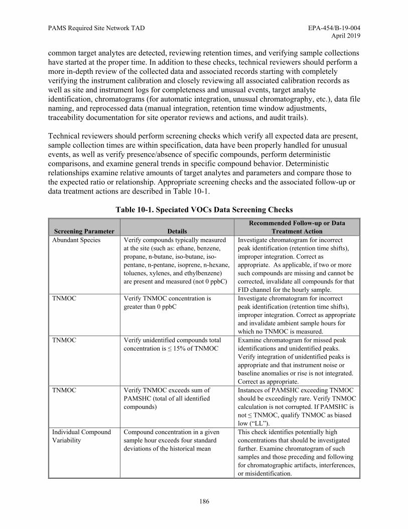
PAMS Required Site Network TAD EPA-454/B-19-004 April 2019
186
common target analytes are detected, reviewing retention times, and verifying sample collections have started at the proper time. In addition to these checks, technical reviewers should perform a more in-depth review of the collected data and associated records starting with completely verifying the instrument calibration and closely reviewing all associated calibration records as well as site and instrument logs for completeness and unusual events, target analyte identification, chromatograms (for automatic integration, unusual chromatography, etc.), data file naming, and reprocessed data (manual integration, retention time window adjustments, traceability documentation for site operator reviews and actions, and audit trails). Technical reviewers should perform screening checks which verify all expected data are present, sample collection times are within specification, data have been properly handled for unusual events, as well as verify presence/absence of specific compounds, perform deterministic comparisons, and examine general trends in specific compound behavior. Deterministic relationships examine relative amounts of target analytes and parameters and compare those to the expected ratio or relationship. Appropriate screening checks and the associated follow-up or data treatment actions are described in Table 10-1.
Table 10-1. Speciated VOCs Data Screening Checks
Screening Parameter Details Recommended Follow-up or Data
Treatment Action Abundant Species Verify compounds typically measured
at the site (such as: ethane, benzene, propane, n-butane, iso-butane, iso-pentane, n-pentane, isoprene, n-hexane, toluenes, xylenes, and ethylbenzene) are present and measured (not 0 ppbC)
Investigate chromatogram for incorrect peak identification (retention time shifts), improper integration. Correct as appropriate. As applicable, if two or more such compounds are missing and cannot be corrected, invalidate all compounds for that FID channel for the hourly sample.
TNMOC Verify TNMOC concentration is greater than 0 ppbC
Investigate chromatogram for incorrect peak identification (retention time shifts), improper integration. Correct as appropriate and invalidate ambient sample hours for which no TNMOC is measured.
TNMOC Verify unidentified compounds total concentration is ≤ 15% of TNMOC
Examine chromatogram for missed peak identifications and unidentified peaks. Verify integration of unidentified peaks is appropriate and that instrument noise or baseline anomalies or rise is not integrated. Correct as appropriate.
TNMOC Verify TNMOC exceeds sum of PAMSHC (total of all identified compounds)
Instances of PAMSHC exceeding TNMOC should be exceedingly rare. Verify TNMOC calculation is not corrupted. If PAMSHC is not ≤ TNMOC, qualify TNMOC as biased low (“LL”).
Individual Compound Variability
Compound concentration in a given sample hour exceeds four standard deviations of the historical mean
This check identifies potentially high concentrations that should be investigated further. Examine chromatogram of such samples and those preceding and following for chromatographic artifacts, interferences, or misidentification.

PAMS Required Site Network TAD EPA-454/B-19-004 April 2019
Table 10-1 (continued). Speciated VOCs Data Screening Checks
187
Screening Parameter Details Recommended Follow-up or Data
Treatment Action Sticking Species has same non-zero value for
three or more consecutive sample hours (this is unlikely to occur typically)
Review affected sample data. This condition may indicate consistent contamination within the instrument such as occurs with aging NafionTM dryers or preconcentrator trap contamination. If contamination is confirmed, invalidate affected target analytes as “SC.”
Benzene : Toluene If benzene concentration exceeds both 3x MDL and toluene concentration (toluene should have a higher concentration)
Ensure correct identification. Flag benzene and toluene as “LJ”
Benzene : Ethane If benzene concentration exceeds both 3x MDL and ethane concentration (ethane should have a higher concentration)
Ensure correct identification. Flag benzene and ethane as “LJ”
Ethylene : Ethane If ethylene concentration exceeds both 3x MDL and ethane concentration (ethane should have a higher concentration)
Ensure correct identification. Flag ethylene and ethane as “LJ”
Propylene : Propane If propylene concentration exceeds both 3x MDL and propane concentration (propane should have a higher concentration)
Ensure correct identification. Flag propylene and propane as “LJ”
o-Xylene : m/p-Xylene If o-xylene concentration exceeds both 3x MDL and m/p-xylenes concentration (m/p-xylenes should have a higher concentration)
Ensure correct identification. Flag all xylenes as “LJ”
2-Methylhexane : 2,3-Dimethylpentane
2-methylhexane concentration should exceed 2,3-dimethylpentane
Review chromatography for interference, proper identification, and integration (no qualification needed)
Methylcyclopentane : 2,4-Dimethylpentane
Methylcyclopentane concentration should exceed 2,4-diemthylpentane
Review chromatography for interference, proper identification, and integration (no qualification needed)
Pentanes Pentanes should show in the following order of decreasing concentration: isopentane, n-pentane, cyclopentane
Review chromatography for interference, proper identification, and integration (no qualification needed)
n-Butane : iso-Butane n-Butane concentration should exceed iso-butane concentration
Review chromatography for interference, proper identification, and integration (no qualification needed)

PAMS Required Site Network TAD EPA-454/B-19-004 April 2019
Table 10-1 (continued). Speciated VOCs Data Screening Checks
188
Screening Parameter Details Recommended Follow-up or Data
Treatment Action Methylpentanes If 3-methylpentane concentration
exceeds both 3x MDL and exceeds 0.6 times the 2-methylpentane concentration Note: 2-Methylpentane and 3-methylpentane elute closely with 2,3-dimethylbutane, as the “terrible trio.” In general, 2-methylpentane should have the highest concentration in ambient air followed by 3-methylpentane then 2,3-dimethylbutane.
Flag 2-methylpentane and 3-methylpentane as “LJ”
Trimethylbenzenes 1,2,3-trimethylbenzene will typically have the highest concentration of the three. 1,3,5-trimethylbenzene and/or 1,2,4-trimethylbenzene should not exceed 1,2,3-trimethylbenzene in ambient air
Review chromatography for interference, proper identification, and integration (no qualification needed)
n-Undecane : n-Decane If n-undecane concentration exceeds both 3x MDL and n-decane (n-decane concentration should be higher)
Flag n-undecane and n-decane as “LJ”
Olefins : Paraffins If sum of olefins concentrations exceeds sum of paraffins concentrations (paraffins concentration sum should be higher)
Flag all olefins and paraffins as “LJ”
Nighttime isoprene Isoprene should not increase in concentration between 8 pm and 3 am local time Isoprene should show a diurnal pattern. Decreases for hourly daytime samples can indicate integration error.
Verify instrument and/or DAS clock, datafile timestamps, and chromatography for misidentifications. If clocks and timestamps are correct and isoprene is correctly identified and integrated, flag isoprene as “LJ” in samples between 20:00 and 03:00.
Decane and undecane If decane and/or undecane are present after nightly QC checks, look for carryover effects indicated by decreasing concentrations in subsequent ambient hourly samples.
If evidence of carryover is confirmed for these compounds, invalidate as “SC.”

PAMS Required Site Network TAD EPA-454/B-19-004 April 2019
Table 10-1 (continued). Speciated VOCs Data Screening Checks
189
Screening Parameter Details Recommended Follow-up or Data
Treatment Action Missing sample data The instrument did not capture an
hourly ambient sample for one or both FID channels
Invalidate compounds from the affected channel missing concentration data as “AF.” Review data from collected sample hour immediately following sample with missing data. If problem affects more than one sample hour, review sample hours through next CCV. Invalidate analytes for sample hours which show problems with “AN” or other appropriate null code.
Sample collection time Sample collection start time began more than 10 minutes before or 30 minutes after the hour, possibly due to wandering instrument clock, DAS clock, computer clock, or problem resulting in delayed instrument “ready” condition.
Invalidate all target analyte concentration data for affected hours as “AG.”
Unusual events documented in site log
Sample collection affected by known source, interference, or event which impacts the representativeness of the sample, such as: vehicle idling near site, landscaping activities, construction equipment in close proximity, leaks in inlet where instrument samples air inside shelter, food truck parked nearby, etc.
Invalidate all target analyte concentration data for affected hours as “SC”.
Confidence is increased in data that pass screening checks, and data that do not meet the defined criteria should be qualified or invalidated as detailed in Table 10-1. For failures of checks for which data qualification or invalidation is not prescribed, these data should minimally be investigated for peak misidentifications, improper integration, or chromatographic artifacts interfering with target analyte peaks, among other problems with the data. Sample hours or lengthy periods of ambient sampling hours failing numerous screening checks may indicate malfunction of the instrument, contamination of the sample, or an error in CDS configuration.
Technical Review should include the following steps:
Examine the collected data for missing data files. Missing files likely point to an instrument failure. For instances of instrument failure, the sample immediately following a missing hour’s sample data is to be invalidated. If possible, data files that are missing due to computer drive mapping problems or inadvertent movement to another location should be recovered so they may be included in the technical review.

PAMS Required Site Network TAD EPA-454/B-19-004 April 2019
190
Review the calibration data:
o Ensure all records are available: COAs, support instrument calibrations, preparation records including dilution measurements or settings, and data files corresponding to analysis of the calibration standards
o Trace the concentrations values entered to generate the calibration curves back to the primary stock COA(s) and associated calculations
o Verify the nominal concentrations entered to generate the calibration curves are accurate to those calculated and verify the curves meet criteria for the linear regression: correlation coefficient, y-intercept, backcalculated values, and RF RSD
o Verify proper assignment of the calibration curve or average RF in the CDS
o Verify the recoveries of the target compounds in the SSCV meet acceptance criteria
Note: The calibration data need only be technically reviewed with the first batch of ambient data measurements. Subsequent ongoing analysis of QC samples will demonstrate the calibration remains valid. Technical reviewers should continue to verify that the correct calibration curve or average RF is programmed into the CDS and that options to update the RF with each CCV are disabled.
Examine summary reports for the ambient sample and QC sample target analyte concentrations and RTs in conjunction with reviewing chromatograms.
o Prepare overlays of the ambient sample data to the daily CCV/RTS to investigate suspected RT shifts
o Examine chromatograms for reference compounds to ensure proper identification
o Verify abundant species are present in ambient sample chromatograms (e.g., ethane, benzene, propane, n-butane, isoprene, n-hexane, and ethylbenzene)
o Examine the results reports for missing components and high concentrations that exceed the calibration curve or detector range
Review results reports and chromatography for the following problems:
o Sample type mismatch between columns (e.g., sample type shows blank on the PLOT FID and ambient sample on the PDMS FID)
o Insufficient collection time or incorrect sample start time (samples collected for fewer than 40 minutes or samples starting earlier than 10 minutes before the hour or later than 30 minutes after the hour)
o GC start times deviate from expectations (should be approximately 40 minutes after sample collection start)
o Sample collection volumes and flows outside of specification.

PAMS Required Site Network TAD EPA-454/B-19-004 April 2019
191
o Instrument malfunction as may be indicated by wild baseline behavior, uncharacteristically broadened peaks, atypical compound elution patterns, or absence of expected compounds
o Mismatch between sample chromatography and sample type (e.g., an ambient sample appears to be a blank or a CCV appears to be an ambient sample)
o Sample data collected as part of instrument conditioning following maintenance or troubleshooting, audit samples, etc.
o Peak responses that exceed the detector range
For samples with responses exceeding the detector range, review chromatograms from samples collected several hours before and after the sample.
o Response could be the result of electronic spiking at the detector or elsewhere in the measurement system. If electronic spiking is suspected, the target analyte concentration should be invalidated. Results may be compared to other nearby sites or other measurement methods (e.g., TO-15) conducted at the site to verify the high concentration, when possible.
o Sample data following high concentration samples can exhibit contamination from carryover and may exhibit RT shifts.
o Daily QC sample data should be reviewed to ensure the system has returned to proper calibration and lack of carryover.
o Compounds with responses exceeding the calibration or detector range will require qualification when reported to AQS (qualify as “EH”).
Review QC sample reports to ensure that daily CCVs and blanks as well as weekly precision checks meet criteria. For QC samples failing criteria, associated ambient data minimally require qualification or may require invalidation for affected compounds. Refer to Table 4-4 of this document.
Perform screening checks as listed in Table 10-1.
Follow up on data that appear to be suspect based on incorrect calculations, missing information, unusual events, acceptance criteria failures, and screening checks. Qualify or invalidate such data as appropriate.
After examining these data reports, organize review notes, pertinent communication with the instrument operator (as applicable), printouts (or saved pdfs, screen shots, or similar) of chromatograms, and any other reviewed information such that they may easily be examined by the data validator. A summary of the technical review including the scope of the data reviewed, high-level observations, and changes or adjustments made to data can streamline operations for subsequent data validation activities. 10.7.3 Speciated VOCs Data Validation Procedures Once data have gone through the data verification processes of routine auto-GC operator review and technical review, the dataset is presumed to be complete and technically correct. Data that

PAMS Required Site Network TAD EPA-454/B-19-004 April 2019
192
have been verified will have been flagged or invalidated based on their suitability and compliance with the governing SOPs. These data can then undergo validation to investigate the internal consistency of the dataset, consistency of the dataset with historical data, and consistency of the dataset with datasets from nearby monitors. 10.7.3.1 Level 1 Data Validation As described previously, tests for internal consistency identify values in the data set that appear atypical when compared to values of the whole data set. Manual data review for internal consistency is impractical for the volume of continuous GC data generated by PAMS. As mentioned previously, DART was designed to review large and complex data sets for consistency. The validator should generate a database of the measured ambient concentrations and QC concentrations over appropriate time periods (e.g., a week, a month, several days, etc.). This generated dataset can be graphed or can be examined for descriptive statistics such as maximum, minimum, median, mean, standard deviation, etc. and evaluate these statistics against expected values. The data validator should also visualize the data with the graphical methods described in Section 10.4. These tools are further described in the following sections as they relate to speciated VOCs data validation. In addition to these generating these statistical values and data visualizations, the data validator should be minimally reviewing the following:
Minimum of three ambient samples for each day
The first and last ambient sample from the time period selected (week, month, etc.)
Ambient samples with the highest TNMOC per channel per day
10% of the QC data for the chosen time period – this includes the daily CCV and system blank as well as the weekly precision check
During review of the data listed above, the validator should review both chromatograms from each channel for:
misidentified samples,
electronic spikes disrupting the chromatogram or affecting target peaks,
samples with obvious baseline abnormalities,
incorrect or inconsistent peak integration,
peak misidentification and missed peak identifications,
co-elutions with target peaks, and
samples with Dean Switch timing errors, where applicable
Validators should prepare overlays of the ambient sample chromatograms with the most recent CCV/RTS to verify that the elution pattern is consistent and that RTs are consistent and stable,

PAMS Required Site Network TAD EPA-454/B-19-004 April 2019
193
and that the auto-GC operator and/or technical reviewer have corrected the data where necessary. Data validators should additionally review site logs, instrument logs, correspondence records, and technical data reviewer notes for additional information related to anomalous sample data, instrument or site issues, or other notable events impacting data. Data validators may widen the scope of their review and select other samples to examine based on the outcome of the review of chromatograms and additional associated information. Data validators may correct data, add qualifiers, invalidate data, or may request that auto-GC operators or technical reviewers perform these actions, based on the privileges defined in the monitoring agency data validation SOP. 10.7.3.2 Level 2 Data Validation - Historical Data Comparisons Note: In the first year following implementation in 2019 many PAMS Required Sites will not have historical data from previous seasons. If possible upon completion of Level 1 validation of the dataset, the data should undergo Level 2 data validation. If monitoring agencies cannot perform Level 2 validation, the dataset should be prepared for uploading to AQS. Testing or comparing data for historical consistency uses many of the graphical techniques discussed in Section 10.4 to compare the dataset with previous data compiled from the monitoring location. The outcome of the Level 2 validation is to identify values for further inspection. Further inspection involves performing reviews of the individual chromatograms and datafiles described in the Level 1 validation for the data identified as questionable. Values representing pollutant behavior outside the determined limits should be flagged for further investigation. 10.7.3.3 Level 3 Data Validation - Parallel Consistency Checks Tests to check for consistency with parallel datasets from the same population (region, period of time, air mass, etc.) are used to identify systematic bias. Systematic bias is determined by checking for the difference in average value or overall distribution values. The sign test, Wilcoxon signed-rank test, Wilcoxon rank sum test, and inter-site correlation tests are recommended for testing two parallel data sets. The first three tests are nonparametric and consequently can be used for non-normal data sets, which frequently occur in air quality data. When comparing VOCs speciation and concentration among nearby sites, observe how well the data compare. Investigate whether differences can be explained by meteorology, photochemistry, analytical instrumentation differences, etc. 10.7.4 Speciated VOCs Visualization Methods 10.7.4.1 Time Series Graphs Time series plots can be used to inspect each target compound, groups of target compounds, and/or TNMOC. These visualizations allow the identification of outliers, increased single-hour concentrations, possible missed peak identifications, and extended periods of unusually high or low concentrations. Experienced PAMS personnel frequently look for unusual “jumps” in the

PAMS Required Site Network TAD EPA-454/B-19-004 April 2019
194
time series plot between successive hourly data or departures from expected diurnal or seasonal patterns. Validators should inspect time-series plots for:
Large “jumps” or “dips” in the concentrations
Periodicity of peaks
Evidence of calibration gas carryover into sample hours following calibration and CCV
Expected diurnal behavior (i.e., biogenic isoprene concentrations usually peak during mid-day or late afternoon)
Expected relationships among species
High single-hour concentrations of less abundant species
Data that appear different than expected should be marked for further investigation. 10.7.4.2 Scatter Plots Scatter plots can be used to compare pairs of target compounds or target groups to identify outliers and excursions in the data such as the improper inclusion of calibration data in the dataset. Prepare scatter plots of the following, at a minimum:
TNMOC versus species groups (i.e., aromatics, paraffins)
TNMOC versus individual species
Benzene versus acetylene and toluene (these species typically correlate)
Benzene versus cyclohexane (look for split in the scatter plot indicating misidentification)
Benzene versus ethane (low or missing ethane concentrations when benzene is abundant may indicate preconcentrator trap problems)
Species that elute close together, e.g., 2,3-dimethylbutane, 2-methylpentane, and 3-methylpentane – 2-methylpentane concentrations should always be the highest of these three peaks in ambient air. These three compounds are prone to misidentification.
Isomers (e.g., o-, m-, and p-xylene).
10.7.4.3 Fingerprint Plots Fingerprint plots allow further inspection of samples previously flagged for more detailed review. The fingerprint plot shows the compound concentration for each compound for a single hour. Prepare the fingerprint plots with VOCs in a consistent order on the x-axis, e.g., retention order, alphabetical order, etc.). The fingerprints can quickly be scanned, hour-by-hour, to allow observation of diurnal changes and inspection of sample hours surrounding suspect data to identify additional effects. 10.7.4.4 Comparison with Other Parameters Other data collected at PAMS sites, such as meteorology data and continuous gaseous measurements, among other sources, may be used to further investigate suspected outliers

PAMS Required Site Network TAD EPA-454/B-19-004 April 2019
195
observed in VOCs data. Following are some examples of evaluations that may clarify the cause of observed outliers:
Plot wind direction data on time series plots – Do extreme values occur from a consistent wind direction?
Produce time series plots with overlays of other criteria pollutant data, such as ozone and NO2 – are there obvious correlations which may explain the anomaly?
Review subsets of data, such as days with high ozone events versus days with lower ozone concentrations.
Investigate local industrial or agricultural operating schedules, unusual event occurrence, etc.
Determine local traffic patterns and understand when peak traffic levels occur.
10.8 Carbonyl Data Verification and Validation During the data verification and validation process for carbonyls, it is useful to consider the various sources of carbonyl compounds in the atmosphere. Aldehydes are both primary pollutants (i.e., directly emitted into the atmosphere) and produced as secondary products of atmospheric photochemistry that also result in ozone production. Because of this relationship, the determination of formaldehyde and other carbonyl compounds in the atmosphere is of interest. Natural sources of carbonyls are not typically abundant; however, aldehydes are commercially manufactured and released into the atmosphere from anthropogenic processes. Acetaldehyde is naturally released during biomass combustion (e.g., wildfires)5 and is produced in biomass decomposition.6 Motor vehicle emissions are a major contributor of atmospheric carbonyls with formaldehyde from vehicle emissions accounting for 50 to 70 percent of the total carbonyl burden to the atmosphere. Furthermore, motor vehicles emit reactive hydrocarbons that undergo photochemical oxidation to produce formaldehyde and other carbonyls in the atmosphere. Similarly, carbonyls are formed during the photo-oxidation of VOCs in the presence of nitrogen oxide. Both anthropogenic and biogenic (e.g., isoprene, pinenes) hydrocarbons result in the formation of carbonyls, especially formaldehyde. Sources of the more abundant carbonyls are listed in Table 10-2.
Table 10-2. Major Sources of Carbonyls in the Atmosphere
Carbonyl Compound Major Source(s) Comments Formaldehyde Fuel combustion key photochemical reaction product (secondary
reaction product) Acetone Surface coating most abundant VOC in landfill emissions and a
product of photochemistry Acetaldehyde Fuel combustion key photochemical reaction product (secondary
reaction product)

PAMS Required Site Network TAD EPA-454/B-19-004 April 2019
196
Carbonyls data are to be verified and validated prior to reporting to AQS. The following sections provide procedures and context for conducting these steps and the acceptance criteria for each performance parameter are listed in Table 10-3. Due to the laboratory component of extraction and analysis, carbonyls data verification and validation will follow a different workflow than the other PAMS Required Site parameters. The monitoring agency is responsible for the sample collection details and the final data validation as it pertains to the site. The ASL is responsible for technical review of the extraction and analysis data. The ASL may perform additional data verification and validation activities depending on the arrangement between the ASL and monitoring agency. Irrespective of the convention, the data verification and validation responsibilities of the ASL and the monitoring agency should be clearly defined as to ensure that all aspects of sample collection, analysis, and data reporting described in the following section are addressed. 10.8.1 Site Operator Verification Activities The site operator should ensure that the sample identifier information and field collection details are properly and completely documented on the sample collection form and/or sample COC and that they conform to the details prescribed in the sample collection SOP during sample setup and collection activities. Sample collection and handling details to document include:
collection date
start and stop times of collection
starting and ending flow rates
duration of collection
dates of sample setup and retrieval
sample shipment and storage records
sampling instrument flow calibration records
Site operators should document observations and unusual events (e.g., situations that may interfere with the sample result, procedural deviations) at the site or with the samples that may impact sample integrity or sample measurement. Prior to releasing the samples to the shipping courier or to the laboratory, the field operator should again verify the sample collection details and COC details are documented completely and accurately, particularly that sample identifier and collection information is correct for field blanks, trip blanks, and duplicate or collocated samples. Site operators are encouraged to maintain a copy of sample collection forms and COC forms for subsequent validation activities. 10.8.2 ASL Verification and Validation Activities 10.8.2.1 ASL Sample Receipt At the laboratory, the sample receipt custodian will complete the custody transfer details and review the sample collection records accompanying the samples to ensure the documentation is complete and reasonable. Inconsistencies (such as sample collection times or volumes that do not

PAMS Required Site Network TAD EPA-454/B-19-004 April 2019
197
seem reasonable) or missing information should be discussed with the field operator to complete or correct the record, as appropriate. The sample custodian should assign a unique identifier, store the samples within the laboratory, and document the sample storage details (refrigerator identifier and maintained temperature range). 10.8.2.2 ASL Sample Extraction The extraction technician will review the sample collection and custody details when preparing the extraction batch to ensure that incomplete or inconsistent information has been corrected and that sample identifiers match. The extraction chemist should document the extraction details sufficiently to ensure that materials used (e.g., extraction solvent, volumetric flasks, spiking solutions) are traceable and that activities (e.g., extract final volume, extract storage) may be reconstructed. Problems or nonconformances with established procedures are to be documented to notify the instrument analyst. 10.8.2.3 ASL Sample Analysis The analyst should review the sample collection and custody records as well as the extraction batch records for notes which may impact the analysis and to ensure records are complete and are associated with the extract sample identifiers. The analyst should document materials utilized (e.g., calibration stocks, mobile phases, volumetric delivery pipettes) and procedures followed (e.g., preparation of calibration standards, analytical methods programs, reagent preparation) to analyze the sample extracts as well as problems or nonconformances with established procedures. Once analysis is completed, the analyst should perform initial (self) review on the analytical data and document adjustments and corrections as needed. This review includes examination of the analytical data and QC sample data to ensure acceptance criteria have been met. The analyst may reanalyze extracts as needed to verify questionable results. Preparation and use of a checklist are recommended to ensure that appropriate analysis procedures and criteria have been addressed. Finally, the analyst should compile a data package which typically includes the associated sample collection and custody forms (or copies thereof), sample extraction records, analysis instrument data, and checklist detailing a summary of the data reviewed and any comments or notes. 10.8.2.4 ASL Overall Technical Review Once the analyst completes their initial review and data package assembly, the data package is then ready for technical review. To streamline the technical review and ensure aspects are not overlooked, a checklist (which can include many of the same details as the analyst checklist) is recommended. Technical review should include the following:
1. Review of the sample collection and custody records
o custody transfer records are complete and reasonable (transfers are chronological)
o sample transport, receipt, and laboratory storage temperatures were ≤ 4°C
o sample collection details are within specifications
start and stop times
beginning and ending, or average flow rates
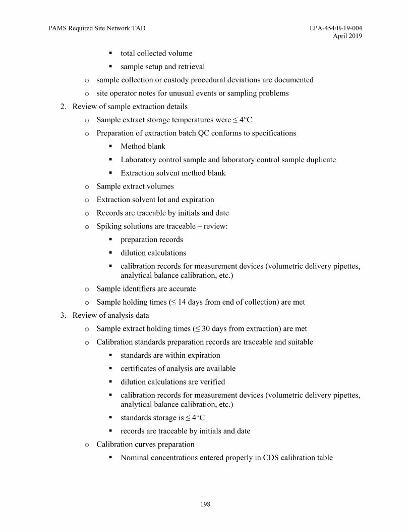
PAMS Required Site Network TAD EPA-454/B-19-004 April 2019
198
total collected volume
sample setup and retrieval
o sample collection or custody procedural deviations are documented
o site operator notes for unusual events or sampling problems
2. Review of sample extraction details
o Sample extract storage temperatures were ≤ 4°C
o Preparation of extraction batch QC conforms to specifications
Method blank
Laboratory control sample and laboratory control sample duplicate
Extraction solvent method blank
o Sample extract volumes
o Extraction solvent lot and expiration
o Records are traceable by initials and date
o Spiking solutions are traceable – review:
preparation records
dilution calculations
calibration records for measurement devices (volumetric delivery pipettes, analytical balance calibration, etc.)
o Sample identifiers are accurate
o Sample holding times (≤ 14 days from end of collection) are met
3. Review of analysis data
o Sample extract holding times (≤ 30 days from extraction) are met
o Calibration standards preparation records are traceable and suitable
standards are within expiration
certificates of analysis are available
dilution calculations are verified
calibration records for measurement devices (volumetric delivery pipettes, analytical balance calibration, etc.)
standards storage is ≤ 4°C
records are traceable by initials and date
o Calibration curves preparation
Nominal concentrations entered properly in CDS calibration table

PAMS Required Site Network TAD EPA-454/B-19-004 April 2019
199
Curves meet acceptance criteria for linearity, intercept, and evaluation against the nominal concentration (criteria listed in Table 5.5)
o Analytical sequence is appropriate
Solvent blank begins the day’s analysis
Calibration is established day of analysis or verified by CCV
Extraction batch QC samples (ESMB, MB, LCS, LCSD)
Sample replicate once per batch
CCV every 12 hours of analysis
Sample identifiers are accurate and traceable
o Compound identification is appropriate
Peak signal to noise is ≥ 3:1
RTs are within the defined RT window
o Peak integration is appropriate and consistent
Automatic integration is reasonable
Coelutions are addressed
Manual integration, where needed, is appropriate, consistent, conforms to monitoring agency procedures and policies, and justified (preferably with documented analyst rationale)
o Dilutions are calculated properly and the MDL is adjusted for (multiplied by) the dilution factor
o Field, extraction, and analysis QC samples meet criteria (listed in Table 5.5)
o Procedural or acceptance criteria failures and corrective actions are documented and justified
o Data reasonability checks performed:
DNPH is present in each cartridge extract (ambient sample, FB, TB, MB, LCS, LCSD) – typically twice the intensity of the next largest peak
Formaldehyde is detected in ambient samples (typically ≥ 0.3 ppbC)
Carbonyl concentrations in ambient samples are reasonable with those expected at the site
o Subsequent calculations for in-air concentrations are correct
o Sample results are qualified appropriately for QC failures or procedural deviations
Laboratories may have additional review requirements including additional levels of technical review, data quality review, or quality assurance assessments before the carbonyls data can be released to the monitoring agency.

PAMS Required Site Network TAD EPA-454/B-19-004 April 2019
200
10.8.3 Carbonyls SLT Monitoring Agency Data Verification and Validation Once the ASL has reported data to the SLT monitoring agency, the monitoring agency data validator can complete the data verification activities and begin validation. Sample data from the ASL may be provided in a number of different formats, depending on the arrangement between the ASL and monitoring site, which may include the following conventions:
simply a mass of target analyte per cartridge (µg/cartridge) for the submitted samples
the mass of target analyte normalized to the collected air volume (µg/m3) for the submitted samples
the mass of target analyte normalized to the collected air volume (µg/m3) in files ready for AQS upload for the submitted samples
the mass of target analyte normalized to the collected air volume in files ready for AQS upload and upload the data to AQS for the submitted samples
Irrespective of the ASL convention for reporting carbonyls field-collected sample (ambient samples and field QC samples such as field blanks and trip blanks) data, the monitoring agency will need to perform subsequent validation on the carbonyls data. The ASL will ensure that the reported values meet the acceptance criteria prescribed in the method and will flag or invalidate data that are compromised per the laboratory QAPP and appropriate SOPs. In addition to the field collected sample data, the ASL may also provide the associated extraction and analytical batch QC data. The monitoring agency data validator should examine these QC data during data validation. Data that are identified as questionable or unsuitable should be discussed with the ASL. 10.8.3.1 Manual Inspection of Carbonyls Collection Data The field operator should have performed initial review of the sample collection data as described in Section 10.8.1 prior to the sample shipment to the ASL. Even if the ASL is reviewing sample collection data, the monitoring agency should also perform technical review of the sample collection and COC forms in concert with the ASL analysis data as part of the data validation. Note that such a technical review is to be performed for each field sampling event to include:
samples collected on the proper date per the national sampling calendar (unless a make-up sample)
leak check performed and passed criteria (as applicable)
pre-sampling purge performed (as applicable)
sampling start and stop times within ±15 minutes of beginning of the scheduled hour (adjusted for clock offset error)
starting, ending, and average flow rates reasonable (e.g., ±10% of setting)
duration of collection within 460 to 500 minutes
sample shipment and storage records – samples stored refrigerated upon retrieval and shipped on ice packs

PAMS Required Site Network TAD EPA-454/B-19-004 April 2019
201
comments on collection forms and/or COC forms that may impact data
COC forms are complete
associated field QC samples meet criteria
If the data validator discovers problems or errors that impact the results, the data validator may need to contact the field operator for clarification or to rectify the problem. Depending on the severity of the issue, the ASL may need to be notified to amend reported data. The data may be corrected effectively, flagged, or invalidated. Refer to Table 10-3 for specific guidance. 10.8.3.2 Review of ASL Data As with manual inspection of the field collected data, the data validator will review the data provided by the ASL for each sampling event for:
sample holding times compliance
acceptable laboratory QC (if provided) and appropriate data flagging
MDLs reported with each sample result
comments or notes affecting data quality
If the data validator discovers problems or errors with the ASL data, the data validator should notify the ASL as soon as practical so the issue can be corrected. The ASL should then provide revised data to the monitoring agency, as appropriate. 10.8.3.3 Review of Supporting QC Data In addition to performing technical review of the routine carbonyls field sampling data, the data validator should review site logs, instrument logs, audit reports, corrective actions, and supporting documentation for the following:
instrument bias checks met criteria at the beginning of PAMS season
sampler siting verified prior to PAMS season
ozone denuder recharged/replaced at the required frequency
sampling instrument flow calibration and calibration verification records demonstrate acceptable performance (within ±10% of transfer standard)
reference transfer standards within calibration
maintenance and site logs detail unusual events
cartridge lot background determination met criteria
cartridge media are within the assigned expiration period
field QC samples collected at the proper frequency
audit findings from IPAs, TSAs, or ADQs affecting data integrity or quality
corrective actions that may impact data integrity or quality

PAMS Required Site Network TAD EPA-454/B-19-004 April 2019
202
A validation table distilling the general QC guidance and requirements for carbonyls is provided in Table 10-3. More information on each data validation parameter can be located within the text identified in the reference column. Each parameter is assigned a category of importance. The categories in order of decreasing importance are:
1. Critical – Criteria will be met for reported results to be valid
2. MQO – PAMS Measurement Quality Objective to be attained to evaluate the DQO
3. Operational – Failure to meet criteria does not invalidate reported results; the results are compromised and on a case-by-case basis may require qualification or invalidation
4. Practical – Failure to meet criteria does not invalidate reported results; results may be compromised, do not require qualification, but may be qualified based on the opinion of the data validator.
Issues or problems with the verifications above and findings or corrective actions impacting data are impetus for data flagging or qualification. Many of the common issues are listed in Table 10-3; however, for situations where a large amount of data is impacted and the guidance does not address the specific situation, monitoring agencies should confer with their Regional representative for how the data should be handled. 10.8.3.4 SLT Monitoring Agency Carbonyls Data Validation Once the carbonyls data have been verified in the above steps, the monitoring agency can conduct validation by employing the statistical and visualization tools and methods described in Section 10.4. 10.8.3.4.1 Level 1 Carbonyls Data Validation Carbonyls data that have undergone data verification will have been evaluated to have met acceptance criteria but should still be examined for suitability by a data validator. Specifically, the data validator should review approximately 5 to 10% of the sample data for transcription and calculation accuracy and verify the criteria in Table 10-3 are met for the chosen samples. Validators should review the following records to assess the impact on the data undergoing validation:
audit records
corrective action reports
monthly flow check results
DNPH cartridge lot blank determinations
sampling unit bias check results
site logbooks
instrument maintenance records

PAMS Required Site Network TAD EPA-454/B-19-004 April 2019
203
field QC sample results
laboratory QC results
These data sources should be examined as a first step in the data validation process and any issues or problems noted should confirm that associated data have been appropriately qualified or invalidated. Provided the supporting data sources discussed above do not indicate anything out of the ordinary, subsequent methods for validating carbonyls data include employing statistical tools to characterize the central tendency and variability and data visualization renderings. Time series plots for formaldehyde and acetaldehyde should be prepared and plots examined for non-detect samples. Formaldehyde should be measured for all ambient (non-field blank) samples above the 0.25 µg/m3 MDL MQO threshold, and acetaldehyde will typically be measured above this level for the two (of the three) sequential samples collected during daylight hours. Concentrations of acetone are highly variable as there are numerous sources including secondary formation (50%), biomass burning (26%), direct biogenic emissions (21%), and anthropogenic sources (3%).5 Additionally, acetone is typically present at significant background amounts on DNPH cartridge media, which complicates the ability to accurately measure the concentration of acetone attributable to ambient measurements. This complication makes it difficult to discern patterns and to assign parameters with which acetone’s behavior correlates or reasonable definitive criteria for determining outliers. Due to the significant and variable acetone background on DNPH cartridges, ambient acetone data may frequently require qualification to estimate the measured concentration, especially when measured in lot blank evaluations, trip blanks, and field blanks. Benzaldehyde may not be measured at concentrations above the MDL due to typically lower atmospheric concentrations relative to formaldehyde and acetaldehyde, therefore atypically high concentrations (e.g., > 0.5 µg/m3) should be reviewed for reasonableness. Preparing plots of the individual compounds for the three different 8-hour periods should indicate a diurnal pattern where the carbonyls concentrations measured in the overnight sample are lowest, particularly for formaldehyde and acetaldehyde. As atmospheric carbonyls burden is primarily driven by mobile sources, time series overlays should be prepared with the BTEX components from the co-collected speciated VOCs data to verify concentrations show a general correlation of increase and decrease together. Scatter plots may be likewise useful in identifying data that deviate from this expected relationship. Carbonyls sample values which deviate significantly from the BTEX trend should be investigated further. A major source of benzaldehyde is as a by-product of atmospheric toluene degradation, particularly in the presence of NO. Benzaldehyde may be compared to daily toluene and/or NO concentrations by preparation of scatter plots. Validators should keep in mind that when comparing data from different measurement systems such as speciated VOCs data, true NO2 data, and meteorological data, the data pulled in for

PAMS Required Site Network TAD EPA-454/B-19-004 April 2019
204
comparison may be in different phases of the data verification and validation process. Validators should be aware that VOCs data may not have gone through validation and may include qualifiers indicating the data quality are compromised. When questionable data are identified by comparison with data from different measurements systems, the data to which they are compared should be quickly reviewed for qualifiers to ensure the comparison is meaningful. Scatterplots and fingerprint plots of carbonyls compounds plotted against speciated VOCs or other carbonyls may be useful in identifying abnormal carbonyls data. Caution should be exercised when combining 8-hour carbonyls data with hourly measurements from continuous methods such that the validator ensures continuous data are plotted on the same time scale (i.e., averaged over the corresponding 8-hour period). Carbonyls data collected as 8-hour samples may be compared generally with 24-hour samples collected over a similar timeframe (e.g., for air toxics networks). Validators should utilize such checks for a gross error check, as the sampling period covers a different time window – 24-hour sampling typically begins and ends at midnight, whereas the 24-hour period for PAMS sampling begins and ends at 04:00 a.m. Additionally, there are known differences in the performance of the collection of carbonyls due to humidity differences. Under identical conditions over the identical time period, a collocated 24-hour sample concentration may differ significantly from the average concentration of three collocated sequential 8-hour samples. Such a gross error check may identify carbonyls compounds or samples for which there are large discrepancies that warrant further investigation. Such may be the case for carbonyls compounds that are measured on one or more of the 8-hour samples but not on the corresponding 24-hour sample. Large, e.g., several-fold, discrepancies may indicate a sample identification discrepancy or measurement error. Such a check may be used to identify data for further investigation but should not in itself be a rationale for invalidation of data. 10.8.3.4.2 Level 2 Carbonyls Data Validation Data validators should compare the current carbonyls dataset against historically collected carbonyls data from the site, if available, to identify values which stand out historically. Comparisons should involve combining the current and historic datasets as possible and generation of simple statistics to identify extreme values and longer-term variability (e.g., standard deviation) that is characteristic at the site and against which outliers may be discerned. Validators should employ the data visualization tools such as time series plots and scatter plots as recommended for the Level 1 validation (overlays with BTEX compounds, etc). Values identified to not conform to the expected pattern should be investigated to verify the values meet criteria or are qualified or invalidated, as appropriate. 10.8.3.4.3 Level 3 Carbonyls Data Validation For Level 3 data validation, carbonyls data should be compared to data generated from other nearby sites within the airshed and collocated samples. When comparing carbonyls concentrations among nearby sites or collocated monitors, observe how well the data compare. Investigate whether differences can be explained by meteorology, photochemistry, analytical instrumentation differences, etc.

PAMS Required Site Network TAD EPA-454/B-19-004 April 2019
205
Table 10-3. Carbonyls Data Validation Table
Parameter Description and Required Frequency Acceptance Criteria Reference Category Field Readiness Checks and Collection Activities
Collection Media All field-collected samples and matrix quality control samples
Cartridge containing silica gel solid sorbent coated with DNPH
Section 5.5 Critical
Media Handling All field-collected samples and all quality control samples
Sample retrieval as soon as possible, not to exceed 72 hours post-sampling. Retrieved sample transported and stored refrigerated at ≤ 4°C, protected from light until extraction. Damaged cartridges (water damage or cracked) must be voided.
Sections 5.8.1.2, 5.5.2, and 5.5.3
Operational
Cartridge Lot Blank Check
Analysis of a minimum of 3 cartridges or 1% of the total lot, whichever is greater, for each new lot
Formaldehyde ≤ 0.15 μg/cartridge, Acetaldehyde ≤ 0.10 μg/cartridge, Acetone ≤ 0.30 μg/cartridge, all others ≤ 0.10 μg/cartridge
Section 5.5.1 and Table 5-2
Critical
Sampling Unit Clock/Timer Check
Verified with each sample collection event
Clock/timer accurate to ± 5 minutes of reference, set to local standard time Sample collection program verified
Section 5.8.1.1 Operational
Sampling Unit Leak Check
Pressurization or evacuation of internal sampler flow paths to demonstrate as leak-free Prior to each sample collection
Must show no indicated flow Section 5.7.2 Operational
Sampling Frequency
Three consecutive 8-hour samples every three days according to the EPA National Monitoring Schedule
Samples in sequence will be valid or a make-up sample sequence scheduled (refer to Section 3.3.2.1)
Section 5.8.1.3 Critical and MQO
Sampling Period All ambient field-collected samples 460 - 500 minutes (8 hr ± 20 mins) starting and ending within 15 minutes of scheduled hour
Section 5.8.1.3 Critical and MQO
Pre-Sample Collection Purge
Prior to the first sequential sample of each sampling event
Minimum of ten air changes just prior to sample collection
Section 5.7.2 Practical

PAMS Required Site Network TAD EPA-454/B-19-004 April 2019
Table 10-3 (continued). Carbonyls Data Validation Table
206
Parameter Description and Required Frequency Acceptance Criteria Reference Category Sample Receipt
Chain-of-custody
All field-collected samples
Each cartridge will be uniquely identified and accompanied by a valid and legible COC with complete sample documentation
Section 5.8.1.4
Critical
Sample Holding Time
All field-collected samples, laboratory QC samples, and standards
Extraction: 14 days from sample collection (cartridge storage ≤ 4 °C) Analysis: 30 days from extraction (extract storage ≤ 4 °C)
Section 5.9.2.4
Operational
Sample Receipt Temperature Check and Subsequent Storage
All field-collected samples upon receipt at the laboratory, stored immediately in refrigerator
≤ 4°C (unless transport duration is not sufficient to sufficiently cool samples)
Section 5.5.2
Operational
HPLC Analysis Solvent Blank (SB)
Prior to ICAL and daily beginning CCV All target compounds ≤ MDLsp Section 5.9.5.2
Operational
HPLC Initial Multi-Point Calibration (ICAL)
Initially, following failed CCV, or when changes to the instrument affect calibration response Analysis of a minimum of 5 points covering approximately 0.01 to 3.0 μg/mL
Correlation coefficient (r) ≥ 0.999; relative error for each level against calibration curve ≤ 20%. Absolute value of intercept divided by slope must not exceed MDLsp
Section 5.9.5.2
Critical
Secondary Source Calibration Verification (SSCV)
Secondary source standard prepared at the mid-range of the calibration curve, analyzed immediately after each ICAL
85 to 115% recovery Section 5.9.5.3
Critical
Continuing Calibration Verification (CCV)
Prior to sample analysis on days when an ICAL is not performed, minimally every 12 hours of analysis, at the end of the analytical sequence - recommended following analysis of every 10 field-collected samples
85 to 115% recovery Section 5.9.5.4
Critical
Extraction Solvent Method Blank (ESMB)
An aliquot of extraction solvent delivered to a volumetric flask. One with each extraction batch of 20 or fewer field-collected samples.
All target compounds ≤ MDLsp Section 5.9.4.1
Operational

PAMS Required Site Network TAD EPA-454/B-19-004 April 2019
Table 10-3 (continued). Carbonyls Data Validation Table
207
Parameter Description and Required Frequency Acceptance Criteria Reference Category Method Blank (MB)
Unexposed DNPH cartridge extracted as a sample One with every extraction batch of 20 or fewer field-collected samples
All target compounds ≤ MDL Section 5.9.4.1
Operational
Laboratory Control Sample (LCS)
DNPH cartridge spiked with known amount of target analytes at approximately the lower third of the calibration curve, twice quarterly - recommended with every extraction batch of 20 or fewer field-collected samples
Formaldehyde recovery 80-120% of nominal spike All other compounds recovery 70-130% of nominal spike
Section 5.9.4.1
Operational
Laboratory Control Sample Duplicate (LCSD)
Duplicate LCS to evaluate precision through extraction and analysis, twice quarterly – recommended with every extraction batch of 20 or fewer samples
Formaldehyde recovery 80-120% of nominal spike All other compounds recovery 70-130% of nominal spike Precision ≤ 20% RPD of LCS
Section 5.9.4.1
Operational
Retention Time (RT)
Every injection Each target carbonyl’s RT within ± 3s or ± 2% of its mean ICAL RT
Section 5.9.5.6
Critical
Replicate Analysis
A single additional analysis of a field-collected sample extract Once with every analysis sequence of 20 or fewer samples
Precision ≤ 10% RPD for concentrations ≥ 0.5 µg/cartridge
Section 5.9.5.5
Operational
Field Blank Minimally twice per month, sample cartridge installed in sampling channel for approximately five minutes to expose the cartridge to the field conditions of the co-collected field sample
Formaldehyde ≤ 0.30 μg/cartridge,Acetaldehyde ≤ 0.40 μg/cartridge,Acetone ≤ 0.75 μg/cartridge, Sum of all other target compounds ≤ 7.0 μg/cartridge
Section 5.8.2.1
Operational
Collocated Sample Collection
Field sample collected through a separate inlet probe from the primary sample 10% of primary samples for sites performing collocated sample collection
Precision ≤ 20% RPD of primary sample for concentrations ≥ 0.5 µg/cartridge
Section 5.8.2.3
Operational
Duplicate Sample Collection
Field sample collected through the same inlet probe as the primary sample 10% of primary samples for sites performing collocated sample collection
Precision ≤ 20% RPD of primary sample for concentrations ≥ 0.5 µg/cartridge
Section 5.8.2.4
Operational

PAMS Required Site Network TAD EPA-454/B-19-004 April 2019
Table 10-3 (continued). Carbonyls Data Validation Table
208
Parameter Description and Required Frequency Acceptance Criteria Reference Category
DNPH Chromatography Evaluation
All cartridges DNPH peak must be presentSection 5.9.5.7
Critical
For all field-collected cartridges DNPH must be ≥ 50% of the DNPH area in the laboratory QC samples
Operational
Laboratory Readiness and Proficiency
Proficiency Testing
Blind sample submitted to each laboratory to evaluate laboratory bias Twice per calendar year, once prior to PAMS season and toward the end of PAMS season 1
Each target compound within ± 25% of the assigned target value
Section 3.3.4.1
Critical and MQO
Method Detection Limit
Determined annually prior to PAMS season and when method changes alter instrument sensitivity
MDL will be: Formaldehyde ≤ 0.25 µg/m3 Acetaldehyde ≤ 0.25 µg/m3
Section 5.6
MQO
Stock Standard Solutions
Purchased stock materials for each target carbonyl All standards
Certified and accompanied by certificate of analysis
Section 5.9.2.2
Critical
Working Standard Solutions And Sample Extracts
Storage of all working standards and extracts Stored at ≤ 4°C, protected from light
Section 5.9.2.4
Operational
Sampling Unit Testing and Maintenance Field Sampler Flow Rate Calibration
Calibration of sampling unit flow controller Minimally annually, prior to PAMS season
Flow set to match a certified flow transfer standard
Table 5.7.1.2
Critical
Ozone Scrubber Recharge
Recharge ozone scrubber with KI Minimally every other PAMS season
Scrubber capacity sufficient to be effective (ozone removal > 95%) for 6 months of 24-hour sampling every third day.
Section 5.4
Critical
Sampling Unit Non-biasing Certification
Verification with humidified zero air or nitrogen that the sampling unit does not contribute to positive bias Prior to field deployment and annually thereafter, or when flow path components are repaired or replaced
< 0.2 µg/cartridge more than the co-collected reference sample for each target carbonyl
Section 5.7.1.1
Operational
Sampling Unit Flow Calibration Check or Audit
Verification of sampling unit flow rate Immediately following calibration and minimally monthly thereafter
Flow within ± 10% of certified primary or transfer standard flow and design flow
Section 5.7.1.2
Operational

PAMS Required Site Network TAD EPA-454/B-19-004 April 2019
Table 10-3 (continued). Carbonyls Data Validation Table
209
Parameter Description and Required Frequency Acceptance Criteria Reference Category Site Specifications and Maintenance
Sampling Unit Siting
Verify conformance to requirements Annually
270° unobstructed probe inlet Inlet 2-15 meters AGL and ≥ 1 meter from any supporting structure ≥ 10 meters from drip line of nearest tree Collocated sampling inlets spaced ≤ 4 meters from primary sampling unit inlet
Section 3.3.1.2
Critical
Sample Probe and Inlet
Sample probe and inlet materials composition Annually
Chromatographic grade stainless steel, PTFE or PFA Teflon®, or borosilicate glass
Section 5.7.3
Critical
Sample Inlet Filter
Particulate filter maintenance Minimally annually prior to PAMS season, if equipped – commensurate with site particulate matter conditions
Clean or replace the inline particulate filter (if equipped)
Section 5.7.3
Operational
Sampling Inlet and Inlet Line Cleaning
Sample inlet and inlet line cleaning or replacement Minimally annually prior to PAMS season - More often in areas with high airborne particulate levels
Cleaned with distilled water or replaced
Section 5.7.3
Operational
Data Reporting
Data Reporting to AQS
Reporting of all results a given calendar quarter Quarterly, within 180 days of end of calendar quarter
All field-collected sample concentrations reported including concentrations below MDL. Field QC sample and laboratory replicates will be reported.
Section 11.2
Operational
AQS Reporting Units
Units as specified with each quarterly submission to AQS µg/m3 or ng/m3 at EPA standard conditions of 25°C and 760 mmHg
Table 11.1 Critical
Data Completeness
Valid samples compared to scheduled samples Each PAMS season
≥ 85% of scheduled samples Section 3.3.2
MQO

PAMS Required Site Network TAD EPA-454/B-19-004 April 2019
210
10.9 Data Verification and Validation of Ozone and Nitrogen Oxides EPA has established data validation guidelines and procedures for data verification and validation for continuous gaseous criteria pollutant (ozone and oxides of nitrogen) monitoring as prescribed in the validation templates in the QA Handbook Volume II, Appendix D, Revision 1, March 2017, available at the following link on AMTIC: https://www3.epa.gov/ttnamti1/files/ambient/pm25/qa/APP_D%20validation%20template%20version%2003_2017_for%20AMTIC%20Rev_1.pdf In general, monitoring agencies will have established data verification and validation procedures for these parameters as part of their criteria pollutant monitoring programs at their NCore monitoring sites. This section will briefly describe some of the aspects of data verification and validation described in Sections 10.1 and 10.2 that apply to the criteria gaseous monitoring, which include:
Timely review of data to correct problems to limit the amount of data affected
Instrument operators and technical reviewers are familiar with the instrument behavior and outputs, typical measured concentrations, typical interferences, calibration routines, and quality control checks and acceptance criteria
Instrument operators should frequently check on the instruments to ensure they are operating properly and that data are being recorded – whether by a site visit or remote login to the instrument or DAS
Data validation should involve calculating simple statistics and visualizing data
Review of the site log and/or instrument log for unusual events and maintenance
Review of independent audits and corrective actions that would indicate ongoing issues impacting data
Documentation of notes, problems, and observations by the data reviewer and validator
For the continuous gaseous criteria measurements, when a zero or span check fails criteria, the ambient measurements recorded should be invalidated back to the most recent passing valid QC check. Data following an analyzer malfunction or period of non-operation should be invalidated until the next calibration or zero and span QC checks unless the QC checks meet criteria and the instrument has not been adjusted over the time in question. For continuous analyzers with on-board or external DAS, including true NO2 and O3, the DAS may include software functions to aid in detecting changes in operating conditions (e.g., sensitivity changes, equipment degradation or malfunction, etc.). As these functions are dependent on the specific instrument model and/or DAS installed, please refer to the manufacturer manual for further information. Such automated validation programs may include the ability to flag data according to:
A user-defined maximum concentration
A user-defined minimum concentration

PAMS Required Site Network TAD EPA-454/B-19-004 April 2019
211
A maximum rate of concentration change
Quality control check failures
Communication errors
10.9.1 Ozone Monitoring agencies should have established guidelines for data review, verification, and validation of ozone. What follows is a summary discussion of ozone data review and validation information described within the EPA QA Handbook Volume II, Appendix D, Revision 1, March 2017. Ozone is a secondary pollutant produced from reactions of NOx and VOCs in the presence of sunlight. Most of the nitrogen oxides emitted into the atmosphere are emitted as NO. If O3 is present where NO is emitted, the O3 levels will be reduced due to NO scavenging (titration). However, in the presence of VOCs, ozone will form and accumulate - over a period of a few hours or over several days, depending on meteorological and other environmental conditions. Typically, a diurnal profile of ozone will show moderate levels overnight, a slight dip as NO levels increase, followed by a steady rise to the maximum ozone value, generally often observed in mid-afternoon, followed by a decay in the early evening when the lack of sunlight, NO, and VOCs limits the production of ozone. Diurnal profiles will vary greatly by site, depending on location, emission sources, and meteorological conditions; they can, however, be useful in identifying unusual/suspect values. Comparison of values to those measured at nearby sites is another useful screening approach. Note that differences observed between nearby sites may be real and should be explainable. For example, if the nearby “buddy” site is further upwind (i.e., closer to a NOx source), the ozone levels may be lower due to titration. Although the relationship between O3 and NO/NO2/NOx/NOy is not definitively predictable, it can be quite useful to plot O3 data with NO2/NOx/NOy. For example, a short-term drop in O3 that appears at the same time as a spike in NOx is likely to be real. Instrument or data transmission issues may be detected by examining the number of hours where the measured ozone concentration is zero. Similarly, instrument issues and/or titration can be indicated by the majority of non-zero values that are less than 30 ppb. Additional screening criteria for ozone are included in Table 10-4. 6
Table 10-4. Example Screening Criteria for Ozone Screening Check Criteria for Further Investigation
Maximum ≥ ~170 to 225 ppbMinimum ≤ ˗5 ppb
Check hourly O3 data for shifts in baseline concentrations Rate of change > 50 to 60 ppb/hrNearby sites Within ± 50 ppbSticking Check > 40 ppb for ≥ 4 consecutive hoursCo-pollutant Relationship with NO and NOx should be conform to expectations

PAMS Required Site Network TAD EPA-454/B-19-004 April 2019
212
10.9.2 Nitrogen Oxides, including True NO2 Monitoring agencies should have established guidelines for data verification and validation of oxides of nitrogen. What follows is a summary discussion of oxides of nitrogen data review and validation information described within the EPA QA Handbook. 7 In the atmosphere, NO2 is generally produced through the reaction of emitted NO with ozone; as such, it can be difficult to establish a relationship between the two compounds. However, it can be useful to plot collocated ozone with NO/NOx/NOy, in a time series plot. The following questions should be considered when screening NO/NOx/NOy data:
Are NO/NO2 concentrations high in the morning and evening?
Are there any negative concentrations?
Do measured values correlate with wind direction for upstream sources?
Additional screening criteria for true NO2 will vary by site; Table 10-5 presents example criteria that can be used as a starting point for developing site-specific criteria. 6
Table 10-5. Example Screening Criteria for NO2/NO/NOx/NOy
Screening Check Criteria for Further Investigation Maximum > 700 ppb urban
>300 ppb ruralMinimum < ˗1 ppbRate of change > 30 ppb/hrSticking Check Any non-zero value for ≥ 4 consecutive hours Co-pollutant NO should not exceed NOx or NOy
NO2 should not exceed NOx or NOy
10.10 Verification and Validation of Routine Meteorological Measurements Ambient air pollution data are linked to meteorological data, and it is strongly recommended that meteorology data be verified and validated at the same time as pollution data. The data verification and validation process for routine meteorological data is described in detail in the EPA QA Handbook, Volume 4, January 2008, available at the following link on AMTIC: https://www3.epa.gov/ttnamti1/files/ambient/met/Volume_IV_Meteorological_Measurements.pdf 10.10.1 Routine Meteorology Data Verification Verification of routine meteorology data includes three basic aspects:
1. routine inspection by site operators of instruments, DAS communication, and data reasonableness
2. automated checks, analysis, and verification performed by the DAS (or similar automated system)

PAMS Required Site Network TAD EPA-454/B-19-004 April 2019
213
3. technical review of data where calibration data, QC check data, and routine data are reviewed for correctness, completeness, and compliance with the established procedures
10.10.1.1 Site Operator Routine Checks Data from certain meteorological parameters can be verified visually. Site operators should check measured meteorological data against manual/visual observations daily when onsite. For example, under windy conditions, a cup anemometer and vane system at a monitoring station should move according to the conditions. Rainfall can be manually inspected using a standard residential precipitation gauge while the site operator is present. Temperature and barometric pressure readings can be checked against measurements from other instruments at the site such as PM2.5 monitors to ensure readings are reasonable. When on site, site operators should perform the following visual checks:
1. Verifying equipment is performing properly and generating reasonable measurements
a. instruments are communicating properly with the DAS
b. mechanical instruments such as wind instruments and precipitation instruments are moving according to conditions and registering reasonable data with the DAS
c. Solar radiation and UV radiation instrument measurements are reasonable for the conditions (sunny, overcast, etc.)
d. Hygrometer readings are reasonable for the conditions (rainy, drought, etc.)
2. The site operator should review the meteorological data collected since the last site visit:
a. Ensure data have been collected for all parameters for all hours
b. Perform a quick visual inspection of the data to look for anomalies from the following expectations:
i. Do higher relative humidity values correspond to relatively high temperature values?
ii. Do temperature reading changes generally transition smoothly?
iii. Are precipitation measurements indicated for recent rain or snow events?
iv. Do solar radiation, UV radiation, and mixing layer height indicate a general diurnal pattern?
Operators should notate observed meteorological conditions when on site and document the checks performed above. An example checklist for routine onsite checks of meteorological instruments is shown in Figure 10-7. This example checklist and a description of what each check entails can be found in the EPA QA Handbook for Air Pollution Measurement Systems Volume IV: Meteorological Measurements Version 2.0, Section 10. Note the form includes a signature block for a reviewer and the completed forms should be reviewed as part of technical data review. Monitoring agencies are encouraged to use this example form, or similar form tailored to the instruments at the site, to record onsite meteorological checks.

PAMS Required Site Network TAD EPA-454/B-19-004 April 2019
214
Figure 10-7. Example Meteorological Sensor Visual Checklist 8

PAMS Required Site Network TAD EPA-454/B-19-004 April 2019
215
Validators will utilize the information recorded on these forms when validating the data collected by the DAS. In addition to the above checks, site operators should review documentation of meteorology instrument calibration to ensure they have recorded calibration activities and reference standards appropriately per the monitoring agency SOP and complete any information gaps as necessary. 10.10.1.2 Data Verification Performed by DAS Monitoring agencies should be conducting data verification activities through checks facilitated through the site DAS. The DAS is configured in advance (e.g., at setup) to establish limits for each parameter to automatically flag data meeting certain criteria; typically these are alarm thresholds established to flag high values, low values, high rates of change, or when data are incomplete. The DAS should be configured such that separate alarm limits are set for instantaneous data and hourly averages. These thresholds should be updated and refined based on the season to include historical data for the season. The suggested DAS automated alarm parameters are shown below for meteorology data:
Values exceeding DAS maximum reading (hardware driven)
Values less than the DAS minimum reading (hardware driven)
Consecutive values exceeding a given maximum rate of change
Values exceeding a seasonal maximum reading (user defined)
Values exceeding a seasonal minimum reading (user defined)
Hourly averages with less than 45 minutes of collected measurements
Monitoring agencies should establish additional parameters and automated checks as appropriate that aid in identifying potential problematic data according to the individual site conditions. Site operators should be performing such checks during routine review and technical reviewers should verify these checks were performed, and if not, conduct them. The automated flags are useful in identifying data that could be problematic, but these data may still be valid for reporting. The reviewer should evaluate whether the flagged data represent meteorological conditions at the site and whether such flagged data should remain flagged. In some cases, extreme meteorological conditions can occur rapidly, and the data may reflect real conditions. For example, if a thunderstorm moves through the site, winds can transition from calm to quickly reach 20 to 30 m/s within seconds and be flagged by the DAS as exceeding a pre-defined rate of change threshold. The reviewer should document the rationale for addressing validity of automatically flagged data and alert data validators that such data were reviewed. 10.10.1.3 Technical Review of Meteorology Data Technical review of meteorology data entails verifying the traceability of the meteorology data from calibration and ensuring the data collection processes are correct and accurate according to the monitoring agency SOPs. Technical reviewers will review the calibration data prior to reviewing the collected environmental data to ensure the documentation trail is traceable, calculations and transformations are accurate, and to ensure:

PAMS Required Site Network TAD EPA-454/B-19-004 April 2019
216
Calibrations were performed at the required frequency and prior to generation of data
Calibration procedures were performed in the proper order as prescribed in the SOP
Calibrations include the proper number of calibration points
Calibration ranges bracket the expected range of reported measurements
Reference standards were within their certified calibration dates (where applicable)
Linearity checks or operational checks were performed (where applicable) to ensure that the measurement system was stable when the calibrations were established
Once the calibration data are verified, technical reviewers should review documentation of QC checks for compliance with acceptance criteria, site logs, instrument maintenance logs, and routine site visit check sheets for completeness and indications of unusual events that may impact data. Technical reviewers should also review routine meteorology data for completeness and verify that missing data or data flagged by the site operator or automatic DAS assessments are appropriately qualified or invalidated. Technical reviewers should document the scope of their review (parameters, date ranges, etc.), the materials reviewed (logs, electronic data, etc.), and activities conducted during technical review so these records are available for data validation. 10.10.2 Meteorology Data Validation Once the data verification process has been completed for meteorology data, the data are presumed to be technically correct and compliant with the established policies and procedures. Data that do not meet technical acceptance criteria will have been qualified (flagged) or invalidated, as appropriate per the monitoring agency policies and procedures. The monitoring agency can then perform Level 1 data validation steps to examine the dataset for internal consistency. 10.10.2.1 Level 1 Validation of Meteorology Data Evaluating the internal consistency of the meteorology data should involve generation of simple statistics to characterize the central tendency and the variability of the data. These statistics are useful in identifying measurement values that appear to be abnormally high or low. As previously discussed, meteorological parameters will fluctuate seasonally, and in general will demonstrate a diurnal pattern, particularly temperature, solar radiation, UV radiation, and mixing layer height. Validators should prepare visualization plots of the meteorology data to aid in identifying extreme values that warrant further investigation. Time series plots are particularly useful in verifying an expected diurnal pattern or rapid changes in values that are not expected. Instrument zero drift may be indicated when the daily minimum values deviate (increase or decrease) from the expected minimum value over a period of several days. Validators should review several consecutive days or weeks of data collected in the early morning hours (e.g., 3 a.m. to 4 a.m.) when winds are light and variable, solar radiation is minimal, and temperatures

PAMS Required Site Network TAD EPA-454/B-19-004 April 2019
217
are typically at their daily minimum. Reviewing daily minimum data over such a time period may reveal a drift in the instrument baseline. Preparing overlays of related meteorological and pollutant parameters on timeseries plots is strongly recommended, including:
Temperature and RH (direct relationship)
Precipitation and RH (direct relationship)
Ozone and ambient temperature (direct relationship)
Wind speed and wind direction
These parameter combinations should also be plotted as scatter plots to identify pairs of data that deviate from the expected relationship. In addition, validators should examine values that standout from visual screening and data flagged by automated DAS screening to confirm they are consistent with a meteorological cause. Site operator and technical reviewer notes should indicate that data flagged by automated DAS screening have been reviewed and the status of validity. Validators should review calibration data and calibration check/QC check data to ensure calibrations were conducted at the proper frequency, adjustments (recalibration) were made when instruments are out of tolerance, and data since the last passing calibration or calibration check were appropriately flagged. Suspect data values may be more closely reviewed and compared to NWS data from nearby stations. Validators should document the scope of the data validated (parameters and date ranges), record observations and actions taken to further investigate suspect data values, and document the outcomes of changes, corrections, or data status changes (such as qualification or invalidation). 10.10.2.2 Level 2 Validation of Meteorology Data For Level 2 validation of meteorological data, the data are compared to historical data at the site to investigate values that stand out historically. It is useful to compare data seasonally by generating simple statistics of historical data and verifying that current measurements are in line with the historical data for the central tendency and variability. Preparing overlays of time series plots of the parameter pairs listed in 10.10.2.1 is useful to identify values that stand out seasonally. Significant deviations from historical measurements may be explained as unusual weather events, or may indicate instrument or data processing problems requiring further investigation and potential data correction, qualification, or invalidation. 10.10.2.3 Level 3 Validation of Meteorology Data Once meteorology data have been validated for Level 1 and Level 2, they should be compared to data from nearby sites, if possible, to investigate systematic bias. While variation is expected due to the unique topographical and geographical nature of each monitoring site, known relationships between sites can be examined. Such relationships may include typical wind directions, temperature gradients, relative humidity conditions due to precipitation run off, and proximity to urban environments or other variables that influence the local microclimates.

PAMS Required Site Network TAD EPA-454/B-19-004 April 2019
218
Comparison of site meteorology data should involve evaluating simple statistics, parameter changes seasonally, and historic data at the sites. Discrepancies between sites are to be expected, but may make extreme values or trends apparent which should prompt closer examination of meteorology data. 10.10.2.4 Reporting Validated Data to AQS Once data validation activities are complete and the data have been verified to be appropriately qualified or invalidated and translated into AQS format, the data may be uploaded to AQS. Once uploaded, the uploaded data should be retrieved and parity checks should be performed to ensure the upload was accurate and complete. Monitoring agencies should maintain documentation of such verifications. 10.11 Using Surface Meteorology Measurements for Data Validation A key advantage to having meteorological data collected onsite is the ability to correlate the occurrence of peak pollutant concentrations to wind conditions. Data analysis of the collected pollutant data will be greatly enhanced by knowing whether winds are calm, parallel to a main pollutant source, or at any other angle positioning the monitoring site relatively upwind or downwind of a known source. In addition, plots of pollutants such as NO2 versus wind speed will generally reveal higher concentrations with lower wind speeds due to reduced dilution of source emissions. Similarly, preparation of pollution roses which plot pollutants as a function of wind direction can reveal patterns in pollutant concentrations from specific wind sectors due to source influences. 10.12 References and Further Reading 1. US EPA. (November 2002). Guidance on Environmental Data Verification and Validation.
EPA QA/G-8 (EPA Publication No. EPA/240/R-02/004). Office of Environmental Information, Washington, DC. Available at (accessed November 2017): https://www.epa.gov/sites/production/files/2015-06/documents/g8-final.pdf
2. http://www.ladco.org/reports/workshops/2011/data_validation/presentations/session_1_intro2011.pdf
3. Guidance for Data Quality Assessment: Practical Methods for Data Analysis: EPA QA/G9: QA00 Update: EPA/600/R-96/084. July 2000. Available at (accessed March 2018:
https://www.epa.gov/sites/production/files/2015-06/documents/g9-final.pdf
4. MacGregor, I.C., Seay, B.S., Selection of an MDL Measurement Quality Objective for Formaldehyde Monitoring in the PAMS Network Based on Historical Measurement Results. US EPA OAQPS Work Assignment 5-07, Project # 100095502, Contract EP-D-13-00510/31/2017
5. Environment Canada and Health Canada. (1999). Canadian Environmental Protection Act. Priority Substances List Assessment Report: Acetaldehyde. ISBN 0-662-28654-5. Cat. No. En40-215/50E. (accessed February 2019). http://publications.gc.ca/site/archivee-archived.html?url=http://publications.gc.ca/collections/Collection/En40-215-50E.pdf
PAMS Required Site Network TAD EPA-454/B-19-004 April 2019
219
6. Kumar, A., Alaimo, C.P., Horowitz, R., Mitloehner, F.M., Kleeman, M.J., Green, P.G. 2011. Volatile Organic Compound Emissions from Green Waste Composting: Characterization and Ozone Formation. Atmospheric Environment Vol. 45: pp 1841-1848. 2011 (accessed February 2019). https://pdfs.semanticscholar.org/1473/f7f0780c407a510a56d70bed59afcc9da402.pdf
7. Singh, H.B., O’Hara, D., Herlth, D., Sachse, W., Blake, D.R., Bradshaw, J.D., Kanakidou, M., Crutzen, P.J. 1994. Acetone in the Atmosphere - Distribution, Sources, And Sinks. J. Geophys. Res.-Atmospheres. 99(D1): 1805-1819. 1994
8. Hafner, H. R. & Cavender, K, 2006, ‘Level 2 Data Validation: Whoops! What the Grass Roots Level Missed’, Presented at The 2006 National Air Monitoring Conference, Las Vegas, NV, November 6-9, 2006 (accessed March 2018). https://www3.epa.gov/ttnamti1/files/2006conference/hafnerdat.pdf
9. US EPA. (January 2017) QA Handbook for Air Pollution Measurement Systems: "Volume II: Ambient Air Quality Monitoring Program" EPA-454/B-17-001 (accessed March 2018). https://www3.epa.gov/ttnamti1/files/ambient/pm25/qa/Final%20Handbook%20Document%201_17.pdf
10. US EPA. (March 2008). Quality Assurance Handbook for Air Pollution Measurement Systems Volume IV: Meteorological Measurements Version 2.0 (Final). EPA-454/B-08-002. Office of Air Quality Planning and Standards, Research Triangle Park, NC. Available at (accessed March 2018): https://www3.epa.gov/ttnamti1/files/ambient/met/Volume_IV_Meteorological_Measurements.pdf

PAMS Required Site Network TAD EPA-454/B-19-004 April 2019
220
11.0 REPORTING DATA TO AQS Following completion of data verification and validation activities, data are to be reported to AQS. Data are to be reported to AQS within 180 days of the end of the calendar quarter in which the measurements were made. During data verification and validation, data which are valid, but which may not have met quality control criteria or are otherwise compromised, will have appropriate qualifier codes added to the data so data users querying data in AQS are informed of any data quality issues. Monitoring agencies should have staff responsible for coding the air monitoring data for AQS and uploading the coded data. 11.1 Coding Ambient and Quality Assurance Data for AQS This section covers reporting of ambient and QA data for carbonyls, speciated VOCs, and meteorology data, as applicable. Monitoring agencies should follow the current approved procedures for the NCore program for reporting the continuous gaseous parameters (ozone, true NO2, NO, and NOy) to AQS. Monitoring agencies will need to amend or add site information and monitors at the PAMS Required Sites to AQS; however, this is a relatively routine function for monitoring agencies to perform, therefore this section will focus on coding and uploading routine ambient and QA data to AQS and will not address AQS transactions used to setup sites and input basic site information or to establish monitors. Additionally, each PAMS Required Site will have data handling practices and procedures defined (in a QAPP, SOP, or similar), which may involve alternative data coding practices for interim database submission, such as is needed for state-operated or regionally-operated databases from which data are subsequently coded for AQS submission. As such, this section describes general aspects for coding data for AQS input. Briefly, AQS accepts data transactions, or inputs, from monitoring agencies for air monitoring data in a pipe-delimited format. These transactions must be programmed in a specific way for AQS to accept the information. The information contained in each data string consist of the following types of information: codes, dates, numeric data, and alphanumeric data. Definitions of these information types are detailed in the AQS Data Coding Manual, Version 3.6, (February 2, 2018), available at the following link: https://www.epa.gov/sites/production/files/2018-02/documents/user_data_coding_manual_feb_2018_0.pdf Each data string, or transaction, consists of a series of fields, each separated by a pipe, “|” to indicate the end of a field and the start of the next field. Depending on the transaction type, some fields may be required and the information in the field must meet specific criteria as defined in the business rules defined in the AQS Data Coding Manual. The EPA has developed an AQS Transaction Generator program that will run in the Windows operating system. This tool facilitates the creation of the AQS transactions and verifies compliance with the AQS data and business rules to ensure the coded transaction will

PAMS Required Site Network TAD EPA-454/B-19-004 April 2019
221
successfully upload to AQS. Note that users will need to have administrator rights on their PC to install the program, available at the following link: https://www.epa.gov/aqs/aqs-transaction-generator Guidance for coding PAMS QA data for submission to AQS is provided in Appendix B. 11.2 Reporting PAMS Parameters to AQS PAMS Required Site monitoring agencies are required to report data for each of the priority chemical parameters listed in Table 2-2 and the meteorological parameters listed in Table 2-3. Monitoring agencies are also encouraged to report data collected for those chemical parameters listed as optional in Table 2-2. Careful attention must be paid to coding of data uploaded to AQS to ensure that the five-digit parameter code is accurate and that the associated units comply with those units AQS accepts. Monitoring agencies are highly encouraged to employ software (e.g., from a DAS, LIMS, or similar) or spreadsheet programs in which the various AQS codes and the data outputs have been validated. Prior to submission of data to AQS, the monitoring agency should have completed data validation and performed a spot check of the dataset to ensure that the parameter code, parameter occurrence code (POC), unit code, method code, and any associated qualifier or null codes are properly assigned. Data which are miscoded may not be identified properly and may result in underestimation of completeness or may be rejected by AQS. PAMS Required Sites will likely have numerous monitors collecting data for monitoring programs besides PAMS. Each individual monitor of a given type (speciated VOCs, carbonyls, true NO2, or meteorology) and duplicate samples collected from a single monitor are assigned a POC by the monitoring agency. There is no guidance on how monitoring agencies assign POCs and discussion with monitoring agencies have indicated several monitors can be assigned the same POC. Data uploaded to AQS indicate the assigned POC, but the POC does not indicate whether the associated data are from a primary monitor, duplicate sample from the primary monitor, or collocated monitor or sample. Due to the ambiguous nature of POC assignment, the monitoring agency should prescribe and maintain a legend of POCs for minimally each of the monitor types required for PAMS Required Site parameters. Monitoring agencies are encouraged to include the POC assignments in their ANP and/or program QAPP. AQS instructions for data upload are described in the AQS User Guide and additional AQS manuals and guides available at the following URL: http://www3.epa.gov/ttn/airs/airsaqs/manuals/ Additional assistance is available by calling the AQS help line at (866) 411-4372. 11.3 AQS Reporting Units Data may be coded with associated units for AQS upload for PAMS parameters in any appropriate unit accepted for that parameter by AQS. Recommended units for reporting data to

PAMS Required Site Network TAD EPA-454/B-19-004 April 2019
222
AQS for each parameter are shown in Table 11-1.
Table 11-1. AQS Parameters and Recommended Reporting Units
Parameter AQS
Parameter Code
Duration AQS
Duration Code
Recommended Reported Unit
AQS Unit Code
Speciated VOCs by Auto-GC refer to
Table 2-2hourly average 1 ppbC 78
True NO2 42602 hourly average 1 ppm 7
Ozone 44201 hourly average 1 ppb 8
Carbonyl Compounds by TO-11A refer to
Table 2-28-hour average 5 µg/m3 at 25°C 1
Ambient Temperature 62101 hourly average 1 °C 17
Relative Humidity 62201 hourly average 1 % relative humidity 19
Barometric Pressure 64101 hourly average 1 millibar (hPa) 16
Wind Speed 61103 hourly average 1 m/s 11
Wind Direction 61104 hourly average 1 degrees compass 14
Solar Radiation 63301 hourly average 1 Watt/m2 79
Ultraviolet Radiation 63302 hourly average 1 Watt/m2 79
Precipitation 65102 hourly average 1 mm 29
Mixing Layer Height 61301 hourly average 1 m 58
Once uploaded to AQS, data may be queried through established reports and different units may be specified; AQS converts to various units specified by the user, as appropriate. For example, carbonyls data may be reported to AQS in µg/m3 but may be converted when queried from AQS as ppbC, ppbV or ng/m3. 11.4 Corrections to Data Uploaded to AQS If it is discovered during data validation, as a result of corrective action, or through other means that erroneous data have been reported to AQS, the data should be corrected and the updated data uploaded to AQS. Situations where this may occur could result in previously acceptable data being invalidated as a result of an audit, or data that were initially incorrectly invalidated could be deemed valid. Monitoring agencies should notify EPA Region staff when a significant amount (as determined by the monitoring agency) of data are discovered and require updating in AQS. Monitoring agencies should coordinate with the EPA Region to correct the records in AQS, as it is important to ensure that data end users are notified of data that may have been updated due to the potential impact on decision-making. 11.5 AQS Qualifiers The monitoring agency should identify compromised data within AQS by addition of a qualifier or combination of qualifiers. Qualifiers associated with PAMS data are indicated in Table 11-2 below. Note that at the time this TAD was published, qualifiers for specific situations were not

PAMS Required Site Network TAD EPA-454/B-19-004 April 2019
223
available in AQS; however, EPA periodically updates the AQS qualifier list which is published at the following link: https://aqs.epa.gov/aqsweb/documents/codetables/qualifiers.html Compromised data should either be flagged or invalidated in AQS as described below. Flagging Data in AQS: Compromised monitoring data will be flagged in AQS only if the data are considered valid for most purposes and uses. AQS permits users to label each data point with up to 10 QA Qualifiers and/or Informational (INFORM) Qualifiers. Invalidating Data in AQS: Data of uncertain origin, data with unacceptable levels of uncertainty, or data which are known to not be an ambient measurement will not have an associated measurement value included in AQS. Such data may be the result of instrument failure, known instrument contamination, irrecoverable data corruption, or measurements associated with failed routine QC checks, calibration, or determination of MDLs or instrument troubleshooting. Invalid data are reported to AQS with a Null (NULL) Code Qualifier which eliminates the associated measurement value and indicates the reason for the invalidation. AQS accepts a single NULL qualifier and does not permit addition of other qualifiers to the transaction string. As discussed further below, data should be qualified and estimated with descriptive QA and INFORM flags where the data are compromised but remain valid. Incorrect use of null codes eliminates the measurement value in the AQS transaction string. Note: EPA intends to add functionality to AQS to automatically add QA qualifier flags to low concentration pollutant data according to their proximity to the MDL.
Table 11-2. AQS Qualifiers for PAMS
Qualifier Code
AQS Qualifier Description Qualifier Type
Comment
1 Deviation from a CFR/Critical Criteria Requirement
QA Substitute a descriptive QA qualifier where possible
2 Operational Deviation QA Substitute a descriptive QA qualifier where possible
3 Field Issue QA Substitute a descriptive QA qualifier where possible
4 Lab Issue QA Substitute a descriptive QA qualifier where possible
5 Outlier QA
7 Below Lowest Calibration Level QA
DI Sample was diluted for analysis QA Applies to carbonyls only
EH Estimated; Exceeds Upper Range QA
FB Field Blank Value Above Acceptable Limit
QA
HT Sample pick-up hold time exceeded QA Applies to carbonyls only
LB Lab blank value above acceptable limit
QA Applies to carbonyls and speciated VOCs

PAMS Required Site Network TAD EPA-454/B-19-004 April 2019
Table 11-2 (continued). AQS Qualifiers for PAMS
224
LJ Identification of Analyte is Acceptable; Reported Value is an Estimate
QA Probably the most common qualifier when an estimate is needed
LK Analyte Identified; Reported Value May Be Biased High
QA Use in place of LJ when direction of bias is known
LL Analyte Identified; Reported Value May Be Biased Low
QA Use in place of LJ when direction of bias is known
MD Value less than MDL QA
ND No Value Detected QA The analyte was not positively identified - should accompany a measurement value of 0
NS Influenced by nearby source QA Rare – in most situations such data should be invalidated
QX Does not meet QC criteria QA
SQ Values Between SQL and MDL QA The SQL is defined as 3.18-fold the MDL value
SS Value substituted from secondary monitor
QA Rare – most sites will not have collocated instruments
SX Does Not Meet Siting Criteria QA Should require invalidation, but no associated null code exists
TB Trip Blank Value Above Acceptable Limit
QA Applies to carbonyls only
TT Transport Temperature is Out of Specs.
QA Applies to carbonyls only
V Validated Value QA Data should be validated when uploaded to AQS, this code is not necessary but may identify suspect values that have gone through additional scrutiny
VB Value below normal; no reason to invalidate
QA
AC Construction/Repairs in Area NULL
AD Shelter Storm Damage NULL
AE Shelter Temperature Outside Limits NULL
AF Scheduled but not Collected NULL
AG Sample Time out of Limits NULL
AH Sample Flow Rate out of Limits NULL Would rather qualify than invalidate
AI Insufficient Data (cannot calculate) NULL Should be used in situations where data were collected for < 75% of the hour or the sampling period for VOCs is < 40 minutes
AM Miscellaneous Void NULL Substitute a more descriptive code where possible
AN Machine Malfunction NULL
AP Vandalism NULL
AQ Collection Error NULL
AR Lab Error NULL
AS Poor Quality Assurance Results NULL Would rather qualify than invalidate, severity dependent
AT Calibration NULL Applies when data represent instrument calibration
AU Monitoring Waived NULL
AV Power Failure NULL
AW Wildlife Damage NULL
AX Precision Check NULL Applies when data represent instrument precision check
AY QC Control Points (zero/span) NULL Applies when data represent instrument QC checks
AZ QC Audit NULL Used for analysis of the VOCs PT sample and TTP audits for ozone and NO2
BA Maintenance/Routine Repairs NULL

PAMS Required Site Network TAD EPA-454/B-19-004 April 2019
Table 11-2 (continued). AQS Qualifiers for PAMS
225
BB Unable to Reach Site NULL
BE Building/Site Repair NULL
BH Interference/co-elution/misidentification
NULL Applies to auto-GC parameters only
BI Lost or damaged in transit NULL Applies to carbonyls only
BJ Operator Error NULL
BK Site computer/data logger down NULL
DA Aberrant Data (Corrupt Files, Aberrant Chromatography, Spikes, Shifts)
NULL
DL Detection Limit Analyses NULL
MC Module End Cap Missing NULL Applies to carbonyls only
SC Sampler Contamination NULL
TC Component Check & Retention Time Standard
NULL
TS Holding Time or Transport Temperature is Out of Specs.
NULL Would prefer to use QA qualifier instead
XX Experimental Data NULL Used for troubleshooting, instrument conditioning, etc
IC Chem. Spills & Indust Accidents INFORM Rare
ID Cleanup After a Major Disaster INFORM Rare
IE Demolition INFORM Rare
IH Fireworks INFORM Rare
II High Pollen Count INFORM Rare
IJ High Winds INFORM Rare
IK Infrequent Large Gatherings INFORM Rare
IM Prescribed Fire INFORM Rare
IP Structural Fire INFORM Rare
IQ Terrorist Act INFORM Rare
IR Unique Traffic Disruption INFORM Rare
IS Volcanic Eruptions INFORM Rare
IT Wildfire-U. S. INFORM Rare
J Construction INFORM Rare
11.5.1 AQS Qualification for Low Concentration Data Concentration data uploaded to AQS will be qualified/flagged according to whether they are above or below the sample quantitation limit (SQL) or method detection limit (MDL) thresholds (refer to Section 3 for further information regarding MDL and SQL). Concentration data less than the determined MDL are to be flagged with the QA qualifier code MD, values greater than or equal to the MDL but less than the SQL (3.18-fold the MDL) are to be flagged using the QA qualifier code SQ. All concentration values for qualitatively (positively) identified analytes, even those less than MDL, are to be reported to AQS and should not be censored by substitution of one half the MDL, by replacement with 0, or by any other substitution method. Negative concentrations should not be translated to zero for reporting purposes. Where qualitative identification acceptance criteria are not met for a given parameter, its concentration must be

PAMS Required Site Network TAD EPA-454/B-19-004 April 2019
226
reported as zero and flagged as ND. The convention for reporting concentration data and the associated QA flags are shown below in Table 11-3.
Table 11-3. AQS Quality Assurance Qualifier Flags for Various Concentrations Compared to a Laboratory’s MDL and SQL
Concentration Level Reported Value Associated AQS QA Flag ≥ SQL measured concentration no flag
≥ MDL and < SQL measured concentration SQ < MDL measured concentration MD
Parameter not qualitatively identified 0 ND
The MDL for a given parameter is to be reported to AQS along with the measured concentration to be a valid AQS transaction string. For carbonyls parameters, the reported MDL should ideally be normalized to the collected air volume for the respective air sample. For example, the target collected air volume for carbonyls sampling at 1.0 L/min is 0.48 m3 and the formaldehyde MDL is 0.098 µg/m3 for this target volume. For a total collected sample volume of 0.42 m3, the MDL is normalized as follows (MDL increases by the ~12% to account of the reduced sample volume): 0.098 µg/m3 ∙ 0.48 m3 = 0.11 µg/m3 0.42 m3

PAMS Required Site Network TAD EPA-454/B-19-004 April 2019
APPENDIX A
EPA ROUNDING GUIDANCE
Provided by EPA Region IV

PAMS Required Site Network TAD EPA-454/B-19-004 April 2019
A-1
Rounding Policy for Evaluating NAAQS QA/QC Acceptance Criteria The following outlines EPA’s Rounding Policy for evaluating Quality Assurance / Quality Control (QA/QC) acceptance criteria. This policy is being provided to air monitoring organizations in order to ensure consistency across the country in the validation of monitoring data that is used for demonstrating compliance with the National Ambient Air Quality Standards (NAAQS). EPA’s interpretation of standard rounding conventions is that the resolution of the measurement device or instrument determines the significant figures used for rounding. The acceptance criteria promulgated in the appendices of 40 CFR Part 50, or otherwise established in EPA guidance documents, are not physical measurements. As an example, the quality control (QC) acceptance criterion of ±5% stated in the fine particulate matter regulations (40 CFR Part 50, Appendix L, Section 7.4.3.1) is not a measurement and, as such, does not directly contribute to either the significant figures or to rounding. However, the flow rate of the sampler – measured either internally by the flow rate control system or externally with a flow rate audit standard – is a measurement, and as such, will contribute to the significant figures and rounding. EPA’s position is that it is not acceptable to adjust or modify acceptance criteria through rounding or other means. Example using PM2.5 Sampler Design Flow Rate 40 CFR Part 50, Appendix L, Section 7.4.3.1 defines the 24-hour sample flow rate acceptance criterion as ±5% of the design flow rate of the sampler (16.67 liters per minute, LPM). The QC acceptance criterion of ±5% stated in regulation is not a measurement and, therefore, does not contribute towards significant figures or rounding. The measurement in this example is the flow rate of the sampler. PM2.5 samplers display flow rate measurements to the hundredths place (resolution) – e.g., 16.67 LPM, which has 4 significant figures. Multiplying the design flow rate (16.67 LPM) by the ±5% acceptance criterion defines the acceptable flow regime for the sampler. By maintaining 4 significant figures – with values greater than 5 rounding up – the computations provide the following results:
The low range is -5% of the design flow: 0.95×16.67=15.8365≈15.84
The upper range is +5% of the design flow: 1.05×16.67=17.5035≈17.50 Rounding in this manner, the lower and upper acceptance limits for the flow rate measurement are defined as 15.84 and 17.50 LPM, respectively. 40 CFR Part 58, Appendix A, Section 3.2.1 requires monthly PM2.5 flow rate verifications. The verification is completed with an independent audit standard (flow device). The monthly check includes a calculation to ensure the flow rate falls within ±5% of the design flow rate (see

PAMS Required Site Network TAD EPA-454/B-19-004 April 2019
A-2
Method 2.12, Section 7.4.7). Therefore, flow rates obtained during monthly flow rate verification checks should measure between 15.84 – 17.50 LPM, as defined above. Measurements, in general, are approximate numbers and contain some degree of error at the outset; therefore, care MUST be taken to avoid introducing additional error into the final results. With regards to the PM2.5 sampler’s design flow rate, it is not acceptable to round the ±5% acceptance criterion such that any calculated percent difference up to ±5.4% is acceptable – because rounding the acceptance criterion increases the error in the measurement. It is important to note that the PM2.5 sampler MUST maintain a volumetric flow rate of approximately 16.67 LPM in order for its inertial separators to appropriately fractionate the collected ambient air particles.
Flow rates greater than 5% of the nominal 16.67 LPM will shift the cut point of the inertial separator lower than the required aerodynamic diameter of 2.5 microns and, thus, block the larger fraction of the PM2.5 sample from being collected on the sample filter. Conversely, as the sampler’s flow rate drops below -5% of the nominal 16.67 LPM, the inertial separator will allow particulate matter with aerodynamic diameters unacceptably larger than 2.5 microns to be passed to the sample filter. Therefore, it is imperative that the flow rate of the sampler fall within the ±5% acceptance criterion. A Note on Resolution and Rounding Measurement devices will display their measurements to varying degrees of resolution. For example, some flow rate devices may show measurements to tenths place resolution, whereas others may show measurements to the hundredths place. The same holds true for thermometers, barometers, and other instruments. With this in mind, rounding should be based on the measurement having the least number of significant figures. For example, if a low-volume PM10 sampler displays flow rate measurements to the tenths place (3 significant figures), but is audited with a flow device that displays measurements to the hundredths place (4 significant figures), the rounding in this scenario will be kept to 3 significant figures. Table 1 below lists some examples of NAAQS regulatory QA/QC acceptance criteria with EPA’s interpretation of the allowable acceptance ranges, as well as a column that identifies results that exceed the stated acceptance limits. Table 1 is not a comprehensive list of ambient air monitoring QA/QC acceptance criteria. Rather, Table 1 is provided to demonstrate how EPA evaluates acceptance criteria with respect to measurement resolution. The validation templates in the QA Handbook Vol II will be revised to meet this policy. If you have any questions regarding this policy or the rounding conventions described, please contact your EPA Regional Office for assistance.

PAMS Required Site Network TAD EPA-454/B-19-004 April 2019
A-3
Table 1: Examples of Quality Control Acceptance Criteria
Regulatory Method
Requirement
Method Acceptance
Criteria
Typical Measurement
Resolution
Acceptance Range (Passing Results)
Exceeding QA/QC Check
Shelter Temperature
20 to 30°C or FEM op. range
1 Decimal, 3 SF*
20.0 to 30.0°C or FEM op. range
≤ 19.9°C ≥ 30.1°C
PM2.5 Design Flow (16.67 lpm)
±5% 2 Decimal, 4
SF 15.84 to 17.50 lpm
≤ -5.1% ≥ +5.1%
PM2.5 Transfer Standard Tolerance
±4% 2 Decimal, 4
SF
-4% Audit Std
Sampler Display
+4% Audit Std
≤ -4.1% ≥ +4.1%
15.84 16.47
16.00 16.67 17.34
16.80 17.50 PM2.5 Lab: Mean Temp 24-hr Mean
20 to 23°C 1 Decimal, 3
SF 20.0 to 23.0°C
≤ 19.9°C ≥ 23.1°C
PM2.5 Lab: Temp Control SD over 24-hr
±2°C 1 Decimal, 3
SF ±2.0°C
≤ -2.1°C ≥ +2.1°C
PM2.5 Lab: Mean RH
24-hr Mean 30% to 40%
1 Decimal, 3 SF
30.0% to 40.0% ≤ 29.9% ≥ 40.1%
PM2.5 Lab: RH Control
SD over 24-hr ±5%
1 Decimal, 3 SF
±5.0% ≤ -5.1% ≥ +5.1%
PM2.5 Lab: Difference
in 24-hr RH Means
±5% 1 Decimal, 3
SF ±5.0%
≤ -5.1% ≥ +5.1%
*SF = Significant Figures

PAMS Required Site Network TAD EPA-454/B-19-004 April 2019
APPENDIX B
AQS Coding Guidance For PAMS Quality Assurance Data

PAMS Required Site Network TAD EPA-454/B-19-004 April 2019
B-1
APPENDIX B: Reporting PAMS QA Data to AQS PAMS QA data reported to AQS includes Blanks and Precision Field QC (Collocated and Duplicate) and Laboratory Samples (Analysis Replicate).
BLANK SAMPLE REPORTING Blank samples for the PAMS program are analyzed for carbonyls by EPA Compendium Method TO-11A and speciated VOCs by auto-GC. Carbonyls Blank Sample Reporting Blank samples for carbonyls in the PAMS program consist of field blanks, trip blanks, lot blanks, laboratory method blanks, and exposure blanks. Monitoring agencies are to report field blank, trip blank, and lot blank data to AQS. Optionally, monitoring agencies may also report laboratory method blanks and exposure blanks. To report blank data, submit a raw blank (RB) transaction for each blank sample. The Blank Types for the various blanks are: Field blank: FIELD Trip blank: TRIP Lot blank: LOT Laboratory Method Blank: LAB Exposure Blank: FIELD 24HR For example, for a field blank, the Blank Type field is entered as “FIELD” (bold in example below). RB|I|11|222|3333|44444|9|7|454|888|FIELD|20150101|00:00|0.0463||||||||||||0.0001|
Speciated VOCs Blank Sample Reporting Blank samples for speciated VOCs in the PAMS program consist of daily system blanks. These blanks are reported similarly to the various blanks collected and analyzed for carbonyls, except the Blank Type is “LAB” to indicate an analysis blank.
PRECISION SAMPLE REPORTING Duplicate and replicate analyses are defined and reported in the PAMS and NATTS programs for carbonyls. Collocated data reporting is used in both the SLAMS and NATTS programs for collocated monitors. The purpose of this section is to clarify how data from these assessments should be reported to AQS using QA transaction formats. (Please note, the old AQS “RA” and “RP” transactions have been retired and can no longer be used to report data.) The goal is to provide consistent reporting terms and procedures to allow the data to be universally understood.

PAMS Required Site Network TAD EPA-454/B-19-004 April 2019
B-2
Simplified schematics are included in this article for illustrative purposes and do not address specifics related to different sampling approaches or methodologies. The AQS transaction formatting descriptions are not repeated in this document, but may be found on the AQS website:
https://aqs.epa.gov/aqsweb/documents/TransactionFormats.html
Collocated Samples Collocated samples are samples collected simultaneously at the same location using two completely separate sampling systems, each with a separate inlet probe to the ambient sampled atmosphere. The allowable distance between inlet probes is defined in regulations or program guidance. Both of the monitors (each designated by a separate AQS Parameter Occurrence Code - POC) have been established in AQS already for the site. The samples are collected and analyzed separately. Each is reported as a sample value for the appropriate monitor. Collocated Sample Schematic
Collocated Sample Reporting Instructions For AQS to automatically create the ‘precision pair’ for the primary and collocated samples, the monitors must be identified to the system as QA collocated. One monitor must be designated as the QA primary. If using transactions, the Monitor Collocation Period (MJ) transaction is used. (If using the AQS application, the “QA Collocation” tab on the Maintain Monitor form may be used to enter these data.) The collocation data must be entered for both monitors, with one indicated as the primary, and the other indicated as the collocated (not the primary). In the example below, the primary monitor is indicated by the bolded ‘Y’ (yes, this is the primary) in the Primary Sampler Indicator in the first MJ string and the collocated monitor by the bolded ‘N’ (no, this is not the primary) in the Primary Sampler Indicator in the second MJ string. Once the monitors have been identified as collocated, there are no additional reporting requirements; simply report the raw data from each monitor (From the schematic, value ‘a’ from

PAMS Required Site Network TAD EPA-454/B-19-004 April 2019
B-3
the primary monitor ‘N’ and value ‘b’ from the collocated monitor ‘C’). Once this is done, AQS will know to pair data from these two monitors for the date range specified. A set of transactions must be created for each time period the monitors are operating together. The transactions have a begin date and end date for the operational period. The end date may be left blank if the collocation period is still active (as indicated in the example below). To define a collocation, submit two MJ transactions (example below with differences bolded and where primary monitor ‘N’ is POC 5 and collocated monitor ‘C’ is POC 9): MJ|I|11|222|3333|44444|5|20150101||3|Y MJ|I|11|222|3333|44444|9|20150101||3|N
Report two Raw Data (RD) transactions for each time sample data are to be reported from both monitors; one for each monitor (POC). (In this example, sample ‘a’ is 0.0463 from monitor ‘N’ (POC 5) and sample ‘b’ from monitor ‘C’ (POC 9) is 0.0458): RD|I|11|222|3333|44444|5|7|454|888|20150101|00:00|0.0463||6||||||||||||0.0001| RD|I|11|222|3333|44444|9|7|454|888|20150101|00:00|0.0458||6||||||||||||0.0001|
Since there are two monitors involved, each sample is reported for its appropriate POC and there will be an RD transaction for every time there is a valid sample from each monitor (e.g., two per day in this scenario). If the sample value from one POC is not available, report a Null data qualifier code for that monitor (that is, do not report the sample value from the collocated monitor as being from the primary POC).
Duplicate Samples Duplicate samples are two (or more) samples collected simultaneously using one or more sampling units sharing a common inlet probe to the ambient atmosphere and the collected samples are analyzed separately. This simultaneous collection may be accomplished by “teeing” the line from the flow control device (sampling unit) to the media (e.g. DNPH cartridges), and then doubling the collection flow rate, or may be accomplished by collecting one discrete sample via two separate flow control devices (sampling units) connected to the same inlet probe, such as two sampling units connected to a common manifold inlet.

PAMS Required Site Network TAD EPA-454/B-19-004 April 2019
B-4
Duplicate Samples Schematic
Duplicate Sample Reporting Instructions In this case, there is only one inlet probe involved but with multiple samples. Since only one inlet probe is involved, all data should be reported for the same POC. First, report the raw data as you normally would via the RD transaction. Report just one value, the one for the sample obtained through the ‘primary’ hardware (the normal flow path or normal cartridge, etc. as defined by the monitoring organization convention – typically this would be sample ‘a’). In this case, if sample ‘a’ comes from the primary hardware and has a value of 54.956, you would report: RD|I|11|222|3333|44444|5|7|454|888|20150101|00:00|54.956||6||||||||||||0.0001|
If the primary value is null for some reason, the duplicate value may be reported as the sample value for this POC in the RD transaction. In this case, there is not a valid duplicate assessment to report. If all duplicates are null, an RD transaction with no sample value and a Null data qualifier code should be reported. Each of the duplicate sample values is then also reported via the QA – Duplicate transaction. This transaction has room for up to 5 duplicate sample values. Report them in any order, starting with 1 and proceeding through the number of samples. In the schematic, there are two samples (a ‘primary’ and a ‘duplicate’) so sample value ‘a’ would be reported as Duplicate Value 1 and sample value ‘b’ would be reported as Duplicate Value 2. The same value reported on the Raw Data transaction must be one of the values reported on the QA – Duplicate transaction.

PAMS Required Site Network TAD EPA-454/B-19-004 April 2019
B-5
Note that there is no sampling time reported on the QA – Duplicate transaction. Instead, there is an Assessment Date and an Assessment Number. If multiple duplicate samples are performed on the same day, label the first with Assessment Number = 1, the second with Assessment Number = 2, and so on. Also note that all values must be reported in the same units of measure. Here is an example QA – Duplicate transaction (with sample ‘a’ = 54.956 and sample ‘b’ = 51.443 – Assessment Number ‘1’ bolded): QA|I|Duplicate|999|11|222|3333|44444|5|20150101|1|454|888|54.956|51.443||||
Replicate Analysis A replicate assessment is a separate analysis or multiple separate analyses of one discrete sample (a carbonyls sample extract) to yield multiple measurements from the same sample. Replicate Analysis Schematic
Replicate Sample Reporting Instructions Again in this case, there is only one AQS monitor (POC) involved and one single sample, however multiple analyses of the sample. First, report the raw data as you normally would via an RD transaction. Report just one value, according to your laboratory’s convention for reporting replicate data (e.g. the first replicate). In this case, if you have chosen replicate ‘a’ as your raw data value and it has a value of 0.844, you would report: RD|I|11|222|3333|44444|5|7|454|888|20150101|00:00|0.844||6||||||||||||0.0001|
If the normally reported value is null for some reason, one of the other replicate values may be reported as the sample value for this POC in the RD transaction. If only one of the replicate values remains valid, there is not a valid replicate assessment to report. If all replicates are null, an RD transaction with no sample value and a Null data qualifier code should be reported. Once the RD transaction is completed, if two or more replicates are valid, these are reported via the QA – Replicate transaction. This transaction has room for up to 5 replicate sample values.

PAMS Required Site Network TAD EPA-454/B-19-004 April 2019
B-6
Report them in any order, starting with 1 and proceeding through the number of samples. In the schematic above there are three replicates ‘a’, ‘b’, and ‘c’ for monitor N, thus analytical value ‘a’ would be reported as Replicate Value 1, analytical value ‘b’ would be reported as Replicate Value 2, and analytical value ‘c’ would be reported as Replicate Value 3. Note that there is no sampling time reported on this transaction. Instead, there is an Assessment Date and an Assessment Number. If multiple replicate samples are collected on the same day, label the first with Assessment Number = 1 (indicated below in bold), the second with Assessment Number = 2, and so on. Also note that all values must be reported in the same units of measure. Here is a sample QA – Replicate transaction (if sample values ‘a’, ‘b’, and ‘c’ are 0.844, 0.843, and 0.792, respectively): QA|I|Replicate|999|11|222|333|44444|5|20210101|1|454|888|0.844|0.843|0.792|||
Combining Duplicates and Replicate Analysis It is possible to collect duplicate samples simultaneously and perform replicate analyses of these duplicate samples. This is often referred to as a duplicate/replicate sample. In this case (see schematic below), there are two duplicate samples, ‘1’ and ‘2’. Duplicate Sample ‘1’ has three replicates: ‘a’, ‘b’, and ‘c’. Duplicate Sample ‘2’ has three replicates: ‘d’, ‘e’, and ‘f’. Replicates of Duplicate Samples Schematic
Duplicate/Replicate Reporting Instructions This scenario requires the reporting of an RD transaction, a QA – Duplicate transaction, and a QA – Replicate transaction to AQS. For the RD transaction, follow the same rules to report the value from the primary (normal) hardware (this would typically be sample ‘1’, replicate ‘a’) and operations procedure path if possible; follow the convention established by the laboratory. If the normal hardware path yields sample ‘1a’ you would report (in this case the value is represented by the “a” in the appropriate place, with spaces for clarity):

PAMS Required Site Network TAD EPA-454/B-19-004 April 2019
B-7
RD|I|11|222|3333|44444|5|7|454|888|20150101|00:00| a ||6||||||||||||0.0001|
For the QA - Duplicate transaction: select one of the replicate analyses each from the primary and duplicate sample (using the convention established by the laboratory) and report those on the QA – Duplicate transaction. If the values to be reported are ‘1a’ and ‘2d’, the record would look like this (again, values are represented by ‘a’ and ‘d’, spaces added for clarity): QA|I|Duplicate|999|11|222|333|44444|5|20210101|1|454|888| a | d ||||
There are only two duplicate samples (one pair) in this case because only two paths were assessed. (That is, you are not allowed to cross-multiply the replicate analyses to create additional duplicate assessments [pairs].) For the replicate transaction: report this as two assessments. Assessment Number 1 for the day would include the values for replicates ‘a’, ‘b’, and ‘c’. Assessment Number 2 for the day would include values for replicates ‘d’, ‘e’, and ‘f’. The example transactions, using letters in place of the values: QA|I|Replicate|999|11|222|333|44444|5|20210101|1|454|888| a | b | c ||| QA|I|Replicate|999|11|222|333|44444|5|20210101|2|454|888| d | e | f |||
Combining Collocated Samples and Replicate Analysis It is also possible to make replicate analyses of collocated samples. These are sometimes referred to as collocated replicate samples. Replicates of Collocated Samples Schematic
Collocated Replicate Reporting Instructions Since collocated monitors report all data independently, report these data for each monitor (e.g., under its own POC) according to the replicate reporting instructions.

PAMS Required Site Network TAD EPA-454/B-19-004 April 2019
B-8
Reporting of Proficiency Test Sample Results Monitoring sites analyzing proficiency test (PT) samples for speciated VOCs and analytical support laboratories (ASLs) analyzing PT samples for carbonyls should report their results to AQS. Proficiency Test Sample Reporting Instructions For the QA – Lab Proficiency Test transaction: The AQS transaction string should be composed as follows: QA|I|Lab Proficiency Test|9999|8888|43502|20180101|1|077|1.21|1.17| where the items described in the sequence are defined as:
QA = quality assurance transaction I = action indicator (insert) Lab Proficiency Test = assessment type 9999 = performing agency 8888 = primary quality assurance organization (PQAO) 43502 = parameter code (formaldehyde in this example) 20180101 = assessment date in format YYYYMMDD 1 = assessment number (should be 1 unless multiple assessments for the same parameter
on the same date) 077 = units (micrograms in this example) 1.21 = laboratory response value 1.17 = assessment mass (assigned PT value)

United States Environmental Protection Agency
Office of Air Quality Planning and Standards Air Quality Assessment Division Research Triangle Park, NC
Publication No. EPA-454/B-19-004 April 2019