ORI GIN AL PA PER

Technical change in a bubble economy: Japanesemanufacturing firms in the 1990s

Takanobu Nakajima Æ Alice Nakamura Æ Emi Nakamura ÆMasao Nakamura

Published online: 17 May 2007

� Springer Science+Business Media B.V. 2007

Abstract An important economic policy issue is to ascertain when and if technical

change (TC) is driving measured growth in productivity. Was this the case for Japan

during the late 1980s when a massive financial bubble was being formed? This paper

addresses this question, after first further developing methods needed for this purpose.

The movement of firms’ TC is of particular policy interest to Japan whose economy has

been suffering from a prolonged recession for more than a decade since the burst of the

bubble in 1990. In the period of time immediately prior to the burst of the bubble, our

estimation results show a significant drop in technical progress. What we believe these

results reflect is that Japanese manufacturing firms made excessive investments in

production inputs in the years when the bubble was being formed. This excessive

investment in inputs did not contribute positively to TC and hence the measured pro-

ductivity and economic growth of the bubble period in the late 1980s was unsustainable.

Keywords Technical change � Total factor productivity � Economies of scale �Japan � Index number method

T. Nakajima

Faculty of Business and Commerce, Keio University, Tokyo, Japan

A. Nakamura

School of Business, University of Alberta, Edmonton, AB, Canada

E. Nakamura

Columbia Business School and Department of Economics, Columbia University, New York, NY,

USA

M. Nakamura (&)

Sauder School of Business, University of British Columbia, Vancouver BC, Canada

e-mail: masao.nakamura@sauder.ubc.ca

M. Nakamura

Institute of Asian Research, University of British Columbia, Vancouver BC, Canada

123

Empirica (2007) 34:247–271

DOI 10.1007/s10663-007-9040-5

JEL classification O3 � O47 � O53 � O49

1 Introduction

An important economic policy issue is to ascertain that technical change (TC) drives

growth in productivity.1 During the late 1980s, several years prior to the burst of the

bubble, the Japanese economy was thought to be enjoying healthy growth and one

of the most profitable periods in Japan’s history.2 Was this growth being driven by

positive TC? This paper addresses this question.3 This is of particular policy interest

to Japan whose economy suffered from a prolonged recession for more than a

decade since 1990.4

Prior to the burst of the bubble in 1990, our estimation results show a significant

drop in technical progress took place. This suggests that the Japanese manufacturing

firms made excessive investment in production inputs in the years prior to 1990

while the bubble was being formed. (The bubble economy may have caused firms to

make such incorrect investment decisions.) Such excessive investment in inputs did

not contribute positively to TC. The growth which was not backed by TC could not

last and the bubble burst in 1990, initiating the prolonged recession. Given the

historically low economic growth rates Japan experienced in the 1990s, such

estimates would be of considerable policy interest.5

1 TC constitutes an integral part of total factor productivity growth (TFPG) but, as discussed below, TC is

not identical to TFPG since the latter contains the effects due to economies of scale.2 A financial bubble is defined here to mean that massive increases in asset prices take place in a short

while without being accompanied by the corresponding increases in their fundamental value. In the

Japanese bubble in the late 1980s the prices of assets such as stocks, land and golf club memberships

increased by several hundred percent or more just within a few years but the Japanese CPI stayed virtually

unchanged during this period. For example, the Nikkei stock average went up from 11,543 in 1985 to

38,922 in January 1990. It collapsed following the burst of the bubble in that year and came down to as

low as 7,907 in 2003. It is still around 16,000. Land prices in Japan followed similar patterns, and they are

still below the 1985 level also. All Japanese banks provided loans using these assets with inflated prices as

collateral to finance households and firms to buy the assets. As soon as the prices of the assets collapsed,

the borrowers ended up with massive loans they could not repay and the Japanese banks ended up with

hundreds of billions of dollars worth of bad (non-performing) loans. Many banks, firms and households

went broke, and the non-performing loans are still troubling the Japanese banks and companies

(particularly in construction and real estate industries) which managed to survive. Japanese manufacturers

did their part in the formation of the bubble. They did not do so much regarding the purchase of inflated

assets but they did borrow massive amounts of funds and this helped fuel the over-expansion of

production capacity.3 This question has not been studied in the literature yet, in part because of the difficulty in estimating TC

while controlling for scale economies.4 The fear of the revival of another financial bubble prevented Japanese government policy makers

involved in both fiscal and monetary policy measures from injecting adequate amounts of cash into the

economy to cope with the serious post-bubble recession. But the lack of their decisive stimulus measures

is thought to have caused the prolonged deflationary trend and less than optimal investment in general.5 For example, the knowledge of the presence of solidly positive TC and returns to scale for the Japanese

manufacturing industries in the 1990s which we find in this paper might have led to a different (and more

stimulating) policy regime than the one that was actually implemented in Japan for coping with the post-

bubble recession.

248 Empirica (2007) 34:247–271

123

In general firms’ total factor productivity growth (TFPG) consists of TC and

economies of scale (the returns to scale), and economies of scale often

systematically vary with the firm characteristics. Our econometric specification

allows estimation of TC and economies of scale separately and hence has some

advantages in testing hypotheses about TC and economies of scale.

In estimating firms’ TC it is important to control for the effects of economies of

scale. But, as discussed below, estimating TC while controlling for scale economies

typically suffers from sample multicollinearity problems.6 In order to avoid such

multicolliarity problems in our estimation, we will use an empirical framework

which takes advantage of certain properties of index numbers.

In this paper we first estimate the TC and scale elasticity (elasticity of scale)

using data on firms in each of 18 Japanese manufacturing industries. TFPG, which is

the sum of TC and economies of scale, is also estimated.

Throughout our estimation work we assume that firms in an industry and given

2-year time period share the same TC and economies of scale parameters. We first

present some evidence that TC for Japanese manufacturing industries declined

significantly in the late 1980s, during the few years prior to the burst of a financial

bubble in 1990. This suggests the existence of massive investments in production

inputs by Japanese manufacturers, where such a capacity expansion was not

accompanied by positive TC. We interpret this to mean that Japanese manufacturers

(like Japanese households and policy makers) were misguided by a financial bubble

being formed in making their investment decisions.

The organization of the rest of the paper is as follows. In the next Sect. 2 we

present our theoretical framework based on which we obtain our econometric

specifications. In Sect. 3 we present our empirical model for estimating TC and

economies of scale using data for firms in Japanese manufacturing industries. We

discuss our data in Sect. 4. In Sect. 5 we present and discuss our estimation results.

Section 6 concludes. Limitations and further extensions of our study are also

discussed in Sect. 6.

2 Theoretical background

It is important to control for returns to scale in estimating TC. This is evidenced by

many previous studies which have reported difficulties in estimating or controlling

for returns of scale in a robust manner. Sample multicollinearity is the primary

reason for such observed difficulties. A standard method to estimate these unknown

parameters is to estimate a flexible cost function using cost share equations.

However, estimating scale economies using a translog cost function,7 for example,

requires estimation of the cost function itself as well as the share equation system.

Since output, its squares and its cross products with input prices are all in the cost

6 This is because regression equations for isolating scale economies by definition require either output or

cost variables on the right-hand side and such variables are often highly correlated with the time trend or

price variables.7 The translog functional form for a single output technology was introduced by Christensen et al. (1971,

1973). The multiple output case was defined by Burgess (1974) and Diewert (1974, p. 139).

Empirica (2007) 34:247–271 249

123

function, multicollinearity can potentially cause serious estimation problems. (For

example, Caves and Barton (1990, p. 34), Chan and Mountain (1983, p. 665) and

Banker et al. (1988, p. 40) report such estimation problems.)

In this study we use an estimating framework that can accommodate a broad

range of underlying production structures while limiting the number of unknown

parameters to be estimated. Our final estimation model contains only a few

explanatory variables which are not highly collinear in cross sections and over time.

Our method, which is parsimonious in terms of the number of unknown parameters

to be estimated, incorporates flexible production functions and provides a

statistically consistent means for estimating scale economies and TC.

We begin by considering the concept of returns to scale in a cross section, and

then go on to allow for disembodied TC over successive 2-year time periods.8

Although the forms of returns to scale and TC that we allow for are simplistic,

estimation is carried out separately at the firm level for each of the eighteen

industries and for each of the two successive years over the 1980s and 1990s. In this

way, we are able to estimate potentially time-varying TC and economies of scale for

manufacturing firms.

2.1 Modeling returns to scale

Our methodology presumes that panel data are available for one or more samples of

production units (PUs, indexed for each sample by i = 1,... ,I), where firms are the

production units in this study. The PUs in each industry are assumed to have the

same production structure for each successive pair of time periods of T years each

(years denoted within each time period as t = 1,... ,T) where T is at least 2.9 In this

study, output for each PU is measured as real sales (denoted by the scalar, yit). On

the input side, data are required for the quantities for N inputs for each PU in each

year (the column vectors xi;t ¼ ðxi;t1 ; . . . ; xi;t

N Þ), and we need unit prices for the inputs

(the column vectors wi;t ¼ ðwi;t1 ; . . . ;wi;t

N Þ). Our firm data are described more fully in

Sect. 4.

For now we ignore the time dimension (and omit the time superscript) so as to

focus on the measure of returns to scale.

To recap, we assume that the structure of production can be described by a

production function f which is homogeneous of degree k, where the constant term

and the returns to scale and technical change parameters are constant for all

individual micro units (firms) in the same industry but are allowed to vary over

industries and from one 2-year time internal to the next.

Thus, for firms in each of our industry, 2-year data samples, we assume that the

structure of production can be described by a homogeneous of degree k production

function denoted by

8 The methodology here can be easily extended to the case where more than two time periods of cross-

sectional data are available.9 In order to allow for the possibility of changing production structures over time, our panels consist of

just two years each (i.e. T = 2); ‘‘rolling’’ 2-year panels. It is not necessary to have a longer panel length.

250 Empirica (2007) 34:247–271

123

yi ¼ f ðxiÞ ð2:1Þ

It follows from the homogeneity assumption for the production function that if

the input vector for the jth PU equals k times the input vector for PU i, then the level

of output for the jth PU is given by k to the kth power times the output quantity for

the PU i; i.e.,

yj ¼ f ðxjÞ¼ f ðkxiÞ¼ kkf ðxiÞ¼ kkyi:

ð2:2Þ

Taking natural logarithms (denoted by ln), from (2.2) we have

ln yj � ln yi ¼ k ln k: ð2:3Þ

Expression (2.3) can be solved for k, yielding

k ¼ ðln yj � ln yiÞ=ln k: ð2:4Þ

This is the elasticity of returns to scale with respect to output for the degree k

homogenous production function f.

For a pair of PUs i and j that have the production structure described by (2.2), k is

the factor by which the input quantities for PU i must be inflated in order to move

from the PU i to the PU j production surface. This is the definition of a Malmquist

input quantity index10 for comparing the inputs of PU i with those of PU j using the

technology of PU i. We denote this Malmquist input quantity index by Q�i;jM ij where

the star indicates that this is an input index, the superscripts following the star

indicate which PUs are being compared, the subscript M indicates that this is a

Malmquist index (the notation M(t) will be used instead when we also wish to note

the time period for the index), and the subscript i indicates that the comparison is

based on the technology of PU i. Similarly, (1/k) is the factor by which the input

quantities for PU j must be equi-proportionately reduced in order to move from the

PU j to the PU i production surface. We also define the Malmquist input quantity

index for comparing the inputs of PU j with those of PU i using the technology of

PU j. We denote this Malmquist input quantity index by Q�j;iM jj .

There is no obvious reason for preferring either Q�i;jM ij or Q�j;iM jj . Thus it is customary

to define the geometric average of these two Malmquist input indexes to be theMalmquist index11 for comparing the inputs of firms i and j, with this Malmquist

10 Diewert and Nakamura (2007) define and discuss the Malmquist output quantity indexes.11 Diewert and Nakamura (2007) explain that the Malmquist output quantity indexes correspond to the

two output indexes defined in Caves et al. (1982, p. 1400) and referred to by them as Malmquist indexes

because Malmquist (1953) proposed indexes similar to these in concept, though his were for the consumer

rather than the producer context. They then go on in the next section to present and discuss Malmquist

input quantity indexes. For more on Malmquist indexes, see Balk (2001), Grosskopf (2003), and Fare

et al. (1994).

Empirica (2007) 34:247–271 251

123

input index denoted equivalently by Q�i;jM or Q�j;iM . Thus, what we will refer to as the

Malmquist input index is given by

Q�i;jM ¼ ðQ�i;jM ij Q

�j;iM jj Þ

ð1=2Þ

¼ Q�j;iM :ð2:5Þ

In the following we present our measurement method, using translog functions,

an important class of flexible production functions.

2.2 Application to a translog production function

In general, Malmquist indexes are theoretical constructs that cannot be evaluated

using observable price data. However, it is well known (e.g., OECD (2001)) that

under certain conditions the Malmquist input index equals the Tornqvist input

quantity index (Theil (1965), Tornqvist (1936) and Fisher (1922)) denoted by

Q�i;jT ð¼ Q�j;iT Þ .12 One of the conditions under which this will be true is when the PUs

have the same translog production function.13 Thus, if f is translog, then we have

k ¼ Q�i;jM ¼ Q�i;jT ð2:6Þ

where

ln Q�i;jT ¼ ð1=2Þðsi þ sjÞ0ðln xj � ln xiÞ ð2:7Þ

Under the additional assumption that the PUs minimize costs, then

si ¼ ðsi1; . . . ; si

NÞ and sj ¼ ðsj1; . . . ; sj

NÞ are the cost share vectors for the N input

factors for the two PUs. The input price vectors for the PUs i and j are denoted by

wi ¼ ðwi1; . . . ;wi

NÞ and wj ¼ ðwj1; . . . ;wj

NÞ, and the elements of the cost share

vectors are given by

sin ¼ ðwi

nxinÞ=ðwi0xiÞ and sj

n ¼ ðwjnxj

nÞ=ðwj0xjÞ ð2:8Þ

where a prime denotes a transpose.14, 15 The Tornqvist input quantity index defined

in (2.7) can be evaluated from the data available to us for firms.

12 Tornqvist indexes are also known as translog indexes following Jorgenson and Nishimizu (1978) who

introduced this terminology because Diewert (1976, p. 120) related the indexes to a translog production

function.13 Using the exact index number approach, Caves et al. (1982, pp. 1395–1401) give conditions under

which the Malmquist output and input volume indexes equal Tornqvist indexes, as noted also in the

OECD (2001) manual on productivity measurement authored by Paul Schreyer, and also in Diewert and

Nakamura (1993).14 Note that the PU specific price vectors are treated as being given exogenously and are assumed not to

depend on the level of production for a PU, though they can vary over the PUs.15 Yoshioka et al. (1994) and Nakajima et al. (1998) presented an alternative proof of (2.6)–(2.8). Their

proof is more indirect than the one given in this paper.

252 Empirica (2007) 34:247–271

123

Suppose that the production function is a homogeneous of degree k translog

function (Christensen, Jorgenson and Lau (1973)) given by

k�1ln f ðxiÞ ¼ b0 þ b01ln xi þ ð1=2Þln xi0R ln xi: ð2:9Þ

In our setting the unknown parameters in (2.9) are b0, a scalar, b1, a column

vector of coefficients with column sum 1, and k, which is a scalar representing the

degree of homogeneity. R is a non-positive definite matrix with column sums equal

to 0. The dimensions of b1 and R conform to that of xi .

For a given time period, if the technology of the PUs i and j can be represented by

the translog production function given in (2.9), then under the assumptions that have

been made and using (2.6), the returns to scale in the cross-section can be

represented as

k ¼ ðln yj � ln yiÞ=ln Q�i;jT

¼ ½ln f ðxjÞ � ln f ðxiÞ�=ln Q�i;jT

ð2:10Þ

where ln Q�i;jT is given by (2.7).

We have shown that when the production functions have flexible translog forms,

the returns to scale parameter k can be described simply as the difference between

the logs of output observed for two sample points divided by the log of the

Tornqvist input quantity index. We will use this fact below for devising econometric

specifications which are parsimonious in the number of unknown parameters to be

estimated.

2.3 Modeling disembodied technical change

In this study, we do not allow for within-industry cross section differences in the

rate of TC and returns to scale (k). In the time dimension, however, we allow both

TC and k to vary from one year to the next for firms in an industry. More

specifically, when modeling the production activities of firms in the same industry

over multiple time periods, we assume a production function that incorporates time

as a separable variable:

yi;t ¼ f ðxi;t; tÞ ¼ k�kf ðkxi;t; tÞ: ð2:11Þ

In this equation, yi;t and xi;t are, respectively, the scalar output quantity and the

production input vector for the ith PU in period t, and k is a positive constant as

before.

We assume that for one time period forward at a time, the technical change of the

PUs can be described, as a first order approximation, by

@ln yi;t=@t ¼ @ln f ðxi;t; tÞ=@t ¼ r ð2:12Þ

where r is a constant. With this assumption, (2.11) can be expressed as

Empirica (2007) 34:247–271 253

123

yi;t ¼ f ðxi;tÞert ð2:13Þ

so that we have

k�1ln yi;t ¼ k�1ln f ðxi;tÞ þ ðk�1Þrt: ð2:14Þ

In (2–14), k�1ln f ðxi;tÞ is assumed to obey the translog function given in (2-9).

3 Empirical methodology

3.1 A basic estimating equation

We assume in the rest of this paper that the translog homogeneous of degree kproduction function characterizes the production environment for firms in an

industry. Suppose that production for the PUs in an industry is described by (2.13),

or

ln yi;t ¼ ln f ðxi;tÞ þ rt: ð3:1Þ

For some reference PU, say A, in some given time period s (1 � s � T � 1) from

(3.1) we have

ln yA;s ¼ ln f ðxA;sÞ þ rs: ð3:2Þ

Now, consider any other PU in time period s, say i. From (3.1) we have

ln yi;s ¼ ln f ðxi;sÞ þ rs: ð3:3Þ

Subtracting (3.3) from (3.2) we have

ln yA;s � ln yi;s ¼ ln f ðxA;sÞ � ln f ðxi;sÞ: ð3:4Þ

Using (2.10), we have the result that

ln f ðxA;sÞ � ln f ðxi;sÞ ¼ k ln Q�A;iTðsÞ ð3:5Þ

where the Tornqvist index on the right compares the inputs for firm i with those for

the reference firm in period s.

For period s+1, the appropriate reference PU for our purposes is A in period s+1,

but with the same input vector as in period s; that is, we use

ln yA;sþ1 ¼ ln f ðxA;sÞ þ rðsþ 1Þ¼ ln yA;s þ r:

ð3:6Þ

Thus for any given period s (1 � s � T � 1), from (3.4) and (3.5) we see that the

period s output for the ith PU is related to the period s output of the reference PU by

254 Empirica (2007) 34:247–271

123

ln yi;s ¼ ln yA;s þ k ln Q�A;iTðsÞ: ð3:7Þ

And for period s+1 we have

ln yi;sþ1 ¼ ln yA;sþ1 þ k ln Q�A;iTðsþ1Þ

¼ ln yA;s þ r þ k ln Q�A;iTðsþ1Þð3:8Þ

where ln yA;sþ1 is the hypothetical expected output of the reference PU in period s+1given by (3-6).

Our basic estimating equation is obtained by combining (3.7) and (3.8) as

ln yi;t ¼ b0 þ b1Di;t þ b2ln Q�A;iTðtÞ þ ui;t ð3:9Þ

where b0 ¼ ln f ðxA;sÞ; b1 ¼ r;b2 ¼ k and where the time dummy is defined by

Di;t ¼ 1 if t ¼ sþ 1

¼ 0 if t ¼ s:ð3:10Þ

The error term u has been added in (3.9) because it is assumed that the derived

estimating equation holds with error for the observed data. In estimation, we treat

the error term ui;t as randomly distributed in the annual cross sections with zero

mean and constant variance r2u and over time (for t = s, s + 1) as autocorrelated with

q as the first order autocorrelation for the PUs in each of our industry and 2-year

subsamples of data for plants and for firms.

There are only three unknown parameters to estimate in our econometric

specification (3.9)16.

In general, year dummy Dit and translog input quantity chain index number Q�A;iTðsÞin (3.9) are not expected to be highly correlated.17 Thus, the proposed specification

will allow us to estimate both r(S) and k(S) with minimal problems from sample

multicollinearity. Since we allow the error term eit in (3.9) to obey a first-order

autoregressive process, we estimate b0, b1 and b2 using generalized least squares

(GLS).18, 19

16 In estimating scale economies and TC using aggregate time series, Chan and Mountain (1983), for

example, had to estimate 22 unknown parameters using 25 annual observations.17 For the particular data sets used, the correlation coefficients calculated for the 18 manufacturing

industries are quite small and range between .009 and .025.18 We carried out the estimation using both OLS and GLS. Since both estimates are similar, only GLS

estimates are presented.19 To estimate (3-9), a reference PU must be selected or created, and then the values must be calculated

for the Tornqvist index for comparing the input quantities of each of the estimation sample PUs with the

input quantities for the reference PU. In this study we have followed the standard method of using as the

reference PU a construct (a hypothetical firm) possessing sample average firm characteristics. (See

Diewert (1999) for more on this sort of approach and the alternatives.) We also used Tornqvist-type input

index values.

Empirica (2007) 34:247–271 255

123

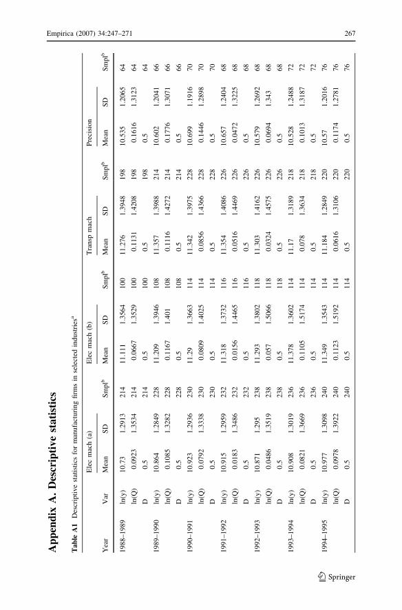
4 Our data and estimation strategy

The primary source of our firm data is the financial statements filed with the

Ministry of Finance and compiled by the Japan Development Bank for manufac-

turing firms listed in the first section of the Tokyo Stock Exchange.20 We use the

following four production inputs: the number of workers (x1) as labor, the fixed

assets at the beginning of each year (x2) as capital, raw material (x3), and other input

goods (x4),21 all measured per firm. Capital (x2) is adjusted for by the industry-

specific capital utilization rate reported by the Japanese Ministry of Economy, Trade

and Industry (METI).

The corresponding input prices used are: the average annual cash earnings per

worker (w1) for x1; the depreciation rate for fixed assets plus the average interest rate

for one-year term-deposit (w2) for x2; the Bank of Japan input price index for the

price of raw materials (w3); and the GDP deflator for the price of other inputs (w4).

Firms’ net sales is used as output (y) and Bank of Japan’s industry output price

index is used as the deflator of output (1988 = 100).

In computing the capital stock x2, new investment in fixed assets is deflated using

the investment goods deflator by industry published by the Economic Planning

Agency. The input price of capital (w2) is also adjusted by the investment goods

deflator. Estimation of (3.9) requires firm output (ln yi,t) and the Tornqvist input

quantity index (ln Q�A;iTðsÞ) which is calculated by (2.7). Descriptive statistics for these

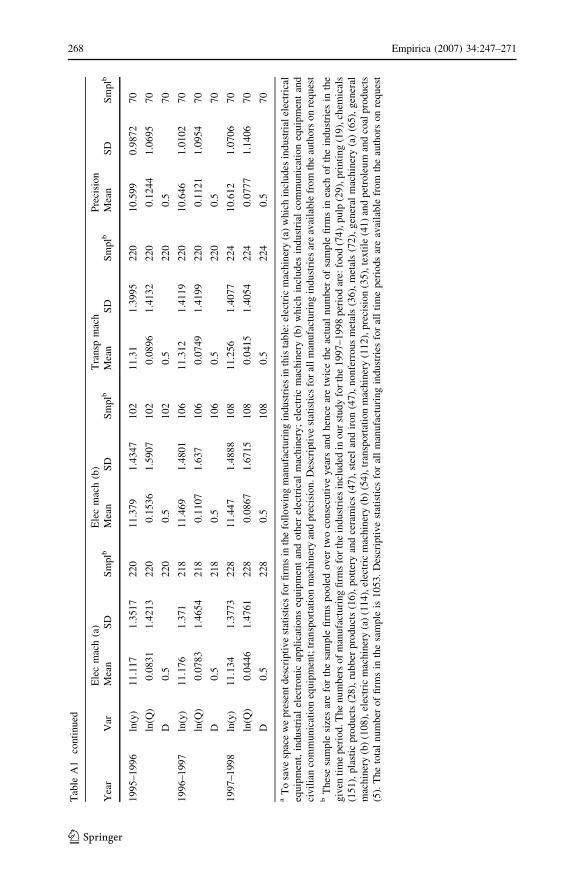
variables are presented for firms in selected industries in Table A1 in Appendix A.22

Since we are interested in the movement of TC over time it is important that our

data set does not suffer from certain sample selectivity problems which might

seriously bias estimation of TC. For example, the movement of R&D expenditures

for our sample firms over time should not be affected due to firms’ entry or exit.

Fortunately our sample consists of large established manufacturers listed in the first

section of the Tokyo Stock Exchange and these firms experienced relatively little

change (in terms of their corporate identity) over our sample time period (1988–

1998). There were only a few major mergers involving firms in this section

(particularly in the petroleum sector), and there were only a few exits of failed firms

which were bought out by other firms and counted as acquisitions. In addition all

our sample firms have positive R&D expenditures.23 For these reasons sample

20 The first section of the Tokyo Stock Exchange lists all established Japanese companies which are

generally much larger than those listed in the second section (for smaller and less established firms) or the

Jasdaq security exchange (for newly created enterprises).21 This is measured on a cost basis and includes all expenses other than the expenses for labor, raw

material and depreciation.22 The numbers of manufacturing firms in our sample for the period 1997–1998 for the industries

included in our study are: food (74), pulp (29), printing (19), chemicals (151), plastic products (28),

rubber products (16), pottery and ceramics (47), steel and iron (47), nonferrous metals (36), metals (72),

general machinery (a) (65), general machinery (b) (108), electric machinery (a) (114), electric machinery

(b) (54), transportation machinery (112), precision (35), textile (41) and petroleum and coal products (5).

The total number of firms in the sample is 1053.23 Also the database we use updates all figures at source so that it contains updated income-statement and

balance-sheet items as well as other financial information items for the firms involved in the acquisitions

that took place in this section during our sample period.

256 Empirica (2007) 34:247–271

123

selection bias does not seem to be a potentially serious problem for our sample and

hence we do not correct for possible selectivity bias in this study.24 Nevertheless we

have done some additional estimation work to verify this. (This is discussed in the

section below on sample selection bias.)

5 Estimation results

5.1 Results using data on firms

Our estimation results for TFPG, TC and the elasticity of scale were derived by the

instrumental variables (IV) method25 for firms in Japanese manufacturing industries

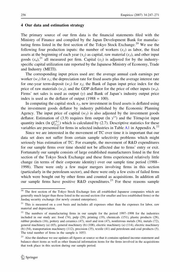
for the period 1988–1998 and are summarized in Tables 1–3, respectively. TC and

the elasticity of scale estimates are also illustrated in Fig. 1. All of the Japanese

manufacturing industries recorded significant reductions in TFP between the 1964–

1988 period and the 1988–1998 period, showing the drastic negative impact of the

burst of the financial bubble in the 1990–1991 period and the subsequent economic

problems on the Japanese manufacturing industries.26 Seven manufacturing

industries (petroleum/coal products, rubber products, steel/iron, electrical machin-

ery (a) and (b), transportation machinery and precision) registered average TFPG

rates above 4% during the 1964–1988 period, with the highest growth rate registered

by electrical machinery (Table 1). Only electrical machinery industries achieved

TFPG of above 2% (i.e., 2.9% and 2.8%) for the period 1988–1998. Of the

remaining industries only textile and plastics registered TFPG above 1% (Table 4).

This is consistent with estimates for Japanese TFP growth using macro series

(Kuroda et al. (2003)).27

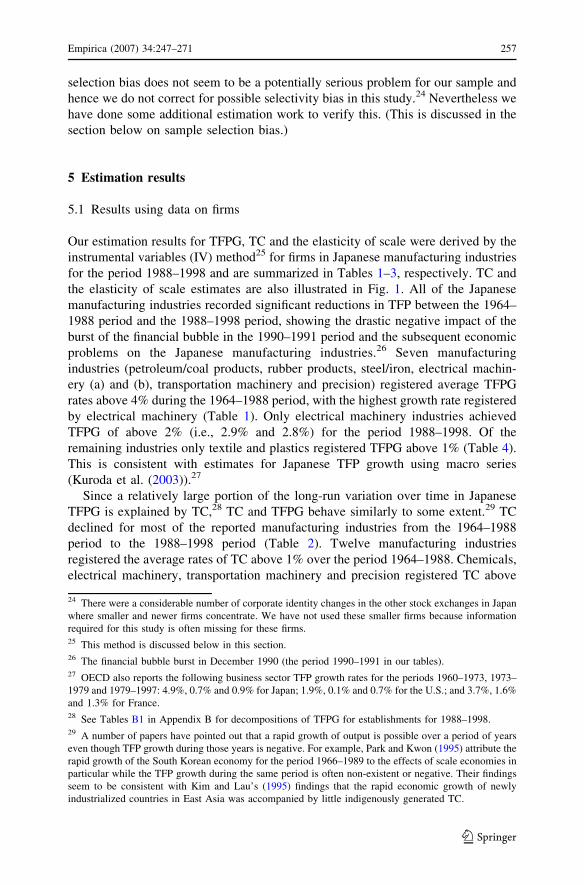
Since a relatively large portion of the long-run variation over time in Japanese

TFPG is explained by TC,28 TC and TFPG behave similarly to some extent.29 TC

declined for most of the reported manufacturing industries from the 1964–1988

period to the 1988–1998 period (Table 2). Twelve manufacturing industries

registered the average rates of TC above 1% over the period 1964–1988. Chemicals,

electrical machinery, transportation machinery and precision registered TC above

24 There were a considerable number of corporate identity changes in the other stock exchanges in Japan

where smaller and newer firms concentrate. We have not used these smaller firms because information

required for this study is often missing for these firms.25 This method is discussed below in this section.26 The financial bubble burst in December 1990 (the period 1990–1991 in our tables).27 OECD also reports the following business sector TFP growth rates for the periods 1960–1973, 1973–

1979 and 1979–1997: 4.9%, 0.7% and 0.9% for Japan; 1.9%, 0.1% and 0.7% for the U.S.; and 3.7%, 1.6%

and 1.3% for France.28 See Tables B1 in Appendix B for decompositions of TFPG for establishments for 1988–1998.29 A number of papers have pointed out that a rapid growth of output is possible over a period of years

even though TFP growth during those years is negative. For example, Park and Kwon (1995) attribute the

rapid growth of the South Korean economy for the period 1966–1989 to the effects of scale economies in

particular while the TFP growth during the same period is often non-existent or negative. Their findings

seem to be consistent with Kim and Lau’s (1995) findings that the rapid economic growth of newly

industrialized countries in East Asia was accompanied by little indigenously generated TC.

Empirica (2007) 34:247–271 257

123

2%. For the 1988–1998 period only electrical machinery achieved the average

rate of TC above 2%. We also note that 12 out of 18 industries registered higher

levels of TC than TFPG for 1988–1998 (Tables 1, 2). This suggests that Japanese

manufacturing firms’ relatively heavier reliance on TC than scale economies in

achieving their TFPG is quite robust. This behavior in TC of Japanese manufac-

turing may provide partial explanations for Japan’s continuing strengths in exports

of manufacturing goods in the 1990s and 2000s. This may deserve further

investigation.

We have also found that the null hypothesis of constant returns to scale (k = 1) is

decisively rejected for firms in most industries and many years in favor of the

alternative hypothesis of decreasing returns to scale (k < 1) for the period 1988–

1998. This is in contrast to the findings at the establishment level that factories in

Table 1 TFP growth (TFPG) for firms in manufacturing industries, 1988–1998a

1964–1988b 1988–1991 1991–1995 1995–1998 1988–1998

Food 0.02167 �0.00464 0.00876 0.00394 0.00329

Textile 0.02281 0.01259 0.03168 0.00753 0.01871

Pulp 0.02961 �0.01245 0.01307 �0.00914 �0.00125

Printing – �0.01051 �0.00802 �0.00340 �0.00738

Chemicals 0.02956 �0.00313 0.00786 0.01186 0.00576

Petroleum/coal products 0.05489 �0.02890 �0.02270 �0.01255 �0.02151

Plastic products – 0.00418 0.03010 0.00200 0.01389

Rubber products 0.04627 0.02911 0.01085 �0.01718 0.00792

Pottery 0.03192 �0.01140 0.00850 0.00345 0.00102

Steel 0.0448 �0.01210 0.00780 0.00091 �0.00024

Non-ferrous metals 0.03759 �0.00416 �0.00191 �0.00443 �0.00334

Metal products 0.03218 �0.04026 0.01868 �0.01084 �0.00786

Gen mach (a)c 0.02707 �0.01506 0.00215 0.01075 �0.00044

Gen mach (b)d 0.02707 �0.00097 �0.00097 �0.00097 �0.00097

Elec mach (a)e 0.05186 0.02690 0.04323 0.01348 0.02941

Elec mach (b)f 0.05186 0.02767 0.02767 0.02767 0.02767

Transp mach 0.04332 0.00645 0.01010 �0.01884 0.00032

Precision 0.04324 �0.00583 0.01187 �0.01053 �0.00016

a This table is based on year-by-year IV regression estimates (available from the authors on request). The

figures given here are the averages calculated for the specified periodsb See Nakajima et al. (1998) for year-by-year regression estimatesc This category includes boilers, engines, metal processing machinery and general machinery partsd This category includes general machinery groupings which are not included in General Machinery (a)e This category includes industrial electrical equipment, industrial electronic applications equipment and

other electrical machineryf This category includes industrial communication equipment and civilian communication equipment

258 Empirica (2007) 34:247–271

123

Japanese manufacturing industries exhibit increasing returns to scale for the period

1968–1998.30 Our findings that the effects of scale economies exist at the

establishment level but disappear at the aggregate level (i.e., firm and industry

levels) imply, among other things, that establishment size does not adjust rapidly

within the time period we consider.

That is, large establishments do not grow at the expense of small establishments.

It is the slowly increasing technical level that explains most of the gains in

aggregate TFP in the Japanese manufacturing sector. Our empirical results suggest

the presence of slow but steady positive TC for the Japanese manufacturing sector.31

Table 2 Technical change (TC) for firms in manufacturing industries, 1988–1998a

1964–1988b 1988–1991 1991–1995 1995–1998 1988–1998

Food �0.0001 �0.00376 0.00535 0.00376 0.00214

Textile 0.0164 0.01332 0.02542 0.00564 0.01585

Pulp 0.0118 �0.01050 0.01442 �0.00330 0.00163

Printing – �0.00902 �0.00826 �0.00255 �0.00677

Chemicals 0.0206 0.00447 0.00791 0.01038 0.00762

Petroleum/coal products 0.0088 �0.03092 �0.02805 �0.01919 �0.02625

Plastic products – 0.01146 0.02048 �0.00074 0.01141

Rubber products 0.0124 0.02949 0.01362 �0.01618 0.00944

Pottery 0.0135 �0.00801 0.00917 0.00160 0.00174

Steel 0.0036 �0.01109 0.00603 �0.00012 �0.00095

Non-ferrous metals �0.0014 �0.00984 �0.00220 �0.00389 �0.00500

Metal products 0.0147 �0.02635 0.01979 �0.01699 �0.00509

Gen mach (a)c 0.0187 �0.00734 0.00242 0.01128 0.00215

Gen mach (b)d 0.0187 0.00108 0.00108 0.00108 0.00108

Elec mach (a)e 0.026 0.03391 0.04799 0.01842 0.03489

Elec mach (b)f 0.026 0.03480 0.03480 0.03480 0.03480

Transp mach 0.0245 0.00907 0.00842 �0.01876 0.00046

Precision 0.0316 0.00159 0.01664 0.00034 0.00724

a This table is based on year-by-year IV regression estimates (available from the authors on request). The

figures given here are the averages calculated for the specified periodsb See Nakajima et al. (1998) for year-by-year regression estimatesc This category includes boilers, engines, metal processing machinery and general machinery partsd This category includes general machinery groupings which are not included in General Machinery (a)e This category includes industrial electrical equipment, industrial electronic applications equipment and

other electrical machineryf This category includes industrial communication equipment and civilian communication equipment

30 Year-by-year estimates for the elasticity of scale for establishments tend to be one (constant returns to

scale) or greater than one (i.e., increasing returns to scale) for most Japanese manufacturing industries for

the period 1963–1998 (see, for example, Nakajima et al. (1998, 2001)).31 Using aggregate time series data for the period 1961–1980 Tsurumi et al. (1986) also find that

Japanese manufacturers spend relatively long periods of time (up to ten years) to adjust their production

methods to incorporate new technological requirements. Their findings are consistent with ours.

Empirica (2007) 34:247–271 259

123

Another reason for the decreasing returns to scale at the firm level is that, while

scale production is still important at the level of individual plants for lowering

production cost, it is becoming increasingly less important in the overall operations

of typical Japanese manufacturing firms. Restructuring and internationalization of

Japanese manufacturers in the 1980s and 1990s resulted in the massive hollow out

of production facilities and their much heavier reliance on revenues from

developments of technologies and new management and manufacturing methods.

Production operations now constitute less than 70% of the total cost of many

Japanese manufacturing firms.32

5.2 Potential endogeneity and IV estimation

In our estimating Eq. (3.9) ln Q�A;iTðtÞ may be correlated with the equation error term

ui,t. To the extent that ln Q�A;iTðtÞ is an index of production inputs, it is less likely to

have such a correlation with the error term than the raw inputs themselves.

Nevertheless, if such a correlation exists and is statistically significant, our OLS

estimates of the equation parameters may be biased. OLS estimates are unbiased

and efficient only if the null hypothesis of no such correlation holds. On the other

hand, IV estimates are consistent even if the null hypothesis does not hold. For this

reason we have estimated Eq. (3.9) using both OLS and IV.33 Since IV estimates are

not efficient, it would be helpful to keep OLS estimates for those cases for which

there is no endogeneity problem. Using standard specification tests34 we have tested

0.0

0.2

0.4

0.6

0.8

1.0

1.2

-0.04 -0.02 0.00 0.02 0.04

TC

elacsf

oyticitsal

E

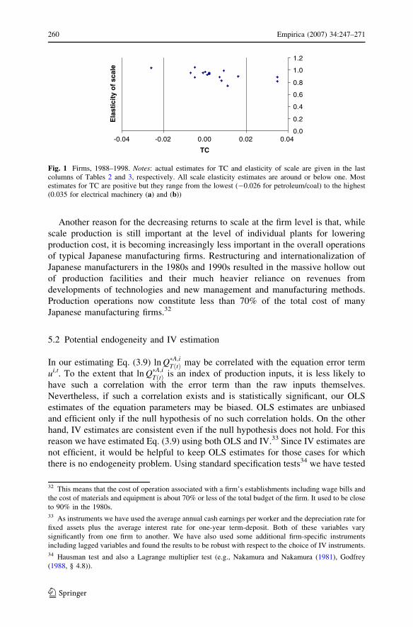
Fig. 1 Firms, 1988–1998. Notes: actual estimates for TC and elasticity of scale are given in the lastcolumns of Tables 2 and 3, respectively. All scale elasticity estimates are around or below one. Mostestimates for TC are positive but they range from the lowest (�0.026 for petroleum/coal) to the highest(0.035 for electrical machinery (a) and (b))

32 This means that the cost of operation associated with a firm’s establishments including wage bills and

the cost of materials and equipment is about 70% or less of the total budget of the firm. It used to be close

to 90% in the 1980s.33 As instruments we have used the average annual cash earnings per worker and the depreciation rate for

fixed assets plus the average interest rate for one-year term-deposit. Both of these variables vary

significantly from one firm to another. We have also used some additional firm-specific instruments

including lagged variables and found the results to be robust with respect to the choice of IV instruments.34 Hausman test and also a Lagrange multiplier test (e.g., Nakamura and Nakamura (1981), Godfrey

(1988, § 4.8)).

260 Empirica (2007) 34:247–271

123

the null hypothesis that there is no endogeneity. The Hausman test rejected the null

hypothesis 9 out of 180 cases (=18 industries · 10 time periods).35 This suggests

that endogeneity is not a serious problem in our sample. Nevertheless, all of our

estimation results for TC presented are IV estimates except for those cases for which

the specification error tests have accepted the null hypothesis of no endogeneity. IV

estimates for TC and the elasticity of scale are summarized in Figure 1.36 Summary

statistics for the decomposition of TFPG into TC and returns to scale are given in

Table B1 in Appendix B.

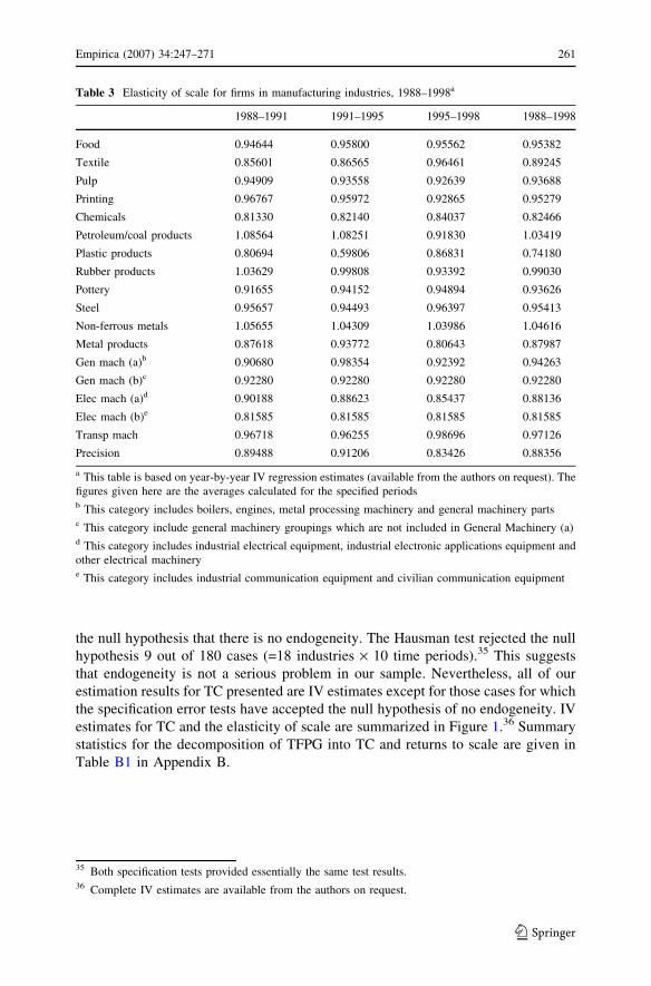
Table 3 Elasticity of scale for firms in manufacturing industries, 1988–1998a

1988–1991 1991–1995 1995–1998 1988–1998

Food 0.94644 0.95800 0.95562 0.95382

Textile 0.85601 0.86565 0.96461 0.89245

Pulp 0.94909 0.93558 0.92639 0.93688

Printing 0.96767 0.95972 0.92865 0.95279

Chemicals 0.81330 0.82140 0.84037 0.82466

Petroleum/coal products 1.08564 1.08251 0.91830 1.03419

Plastic products 0.80694 0.59806 0.86831 0.74180

Rubber products 1.03629 0.99808 0.93392 0.99030

Pottery 0.91655 0.94152 0.94894 0.93626

Steel 0.95657 0.94493 0.96397 0.95413

Non-ferrous metals 1.05655 1.04309 1.03986 1.04616

Metal products 0.87618 0.93772 0.80643 0.87987

Gen mach (a)b 0.90680 0.98354 0.92392 0.94263

Gen mach (b)c 0.92280 0.92280 0.92280 0.92280

Elec mach (a)d 0.90188 0.88623 0.85437 0.88136

Elec mach (b)e 0.81585 0.81585 0.81585 0.81585

Transp mach 0.96718 0.96255 0.98696 0.97126

Precision 0.89488 0.91206 0.83426 0.88356

a This table is based on year-by-year IV regression estimates (available from the authors on request). The

figures given here are the averages calculated for the specified periodsb This category includes boilers, engines, metal processing machinery and general machinery partsc This category include general machinery groupings which are not included in General Machinery (a)d This category includes industrial electrical equipment, industrial electronic applications equipment and

other electrical machinerye This category includes industrial communication equipment and civilian communication equipment

35 Both specification tests provided essentially the same test results.36 Complete IV estimates are available from the authors on request.

Empirica (2007) 34:247–271 261

123

5.3 Potential sample selection bias

One of the objectives of this study is to analyze the movement of TC characterizing

large Japanese manufacturers. Because of its massive influence on the growth of the

Japanese economy, the movement of TC for large manufacturers is of serious policy

concern to government policy makers.37 For this reason our sample firms consist of

generally established large manufacturing firms listed in the first section of the

Tokyo Stock Exchange. The sources of potential sample selection bias of the sorts

Heckman (1976, 1979) considers include entry and exit into the sample of interest,

corporate identity changes due to mergers and acquisitions, and a censored or

truncated R&D variable. Because our sample firms are all large and established,

they all conduct R&D and hence we have no truncation problem from this source. It

is also the case that, because of the prevalence of Japanese corporate governance

and management practices,38 very few mergers, acquisitions and takeovers (hostile

or friendly) take place between large Japanese firms.39 In addition new entries to or

exits from the first section of the Tokyo Stock Exchange have been a relatively rare

event.40 For these reasons, the composition of firms in the included industries over

our sample period (1988–1998) changed relatively little.41 The actual variation over

ten time periods in the number of firms included in our sample is reported for some

selected industries in Table B1; this information can be summarized as follows:

food (minimum size = 73, maximum size = 98); pulp (26, 31), printing (9, 19),

chemicals (144, 160), plastic (144, 160), rubber (16, 19), pottery and ceramic (48,

59), steel and iron (47, 52), non-ferrous metals (35, 39), metals (49, 72), general

machinery (a) (63, 71), general machinery (b) (96, 109), electrical machinery (a)

(107, 120), electrical machinery (b) (50, 59), transportation machinery (99, 114),

precision instruments (32, 38), textiles (38, 49) and petro and coal (5, 10).42

Our estimation method (3.9) allows us to use as many firms for each 2-year

estimating panel as we have data for. This characteristic of our estimation method is

37 Many policy makers believe, correctly or incorrectly, that these large firms drive Japan’s economic

growth.38 See, for example, Morck and Nakamura (1999) and Morck et al. (2000).39 For example, after having agreed to merge on friendly terms in order to gain international

competitiveness, the Mitsui Chemical and Sumitomo Chemical Companies (Japan’s second and third

largest chemical firms) decided not to merge last year. Their reason was the incompatibility of the firm-

specific management methods of the respective companies.40 Permission to be listed on this stock exchange requires a significant amount of accomplishment on the

part of the applicant firm. Few firms, once listed, exit from it.41 Also the sample size varies only slightly from one period to another for most industries (Table B1).42 The variation in the sample size comes primarily from the occasional lack of relevant data for a few

companies in each of the industries. The major exceptions are: the petroleum industry in which, because

of the substantial rise in oil price in recent years, major mergers took place: the printing industry in which

some large firms listed their former divisions involved in printed circuit-related business lines; and the

food industry in which some existing firms also separated and listed some of their divisions for new

products.

262 Empirica (2007) 34:247–271

123

particularly useful for one of the objectives of our study: to measure the over time

evolution of TC with reasonable efficiency. Nevertheless, in order to access the

potential impact of this variation in sample size over time on our empirical results,

we have also estimated (3.9) using a panel of firms which appear in each of the ten

time periods. (By definition the number of firms in the panel for each industry is the

minimum of the two numbers given for that industry above.) The results using this

panel data are almost identical to those we obtained earlier. This suggests that the

type of variation we have in the number of firms included in the 2-year panel is not a

serious source of sample bias.43

5.4 The bubble

In the late 1980s when a financial bubble was being formed, the Japanese economy

was thought to be enjoying the best prosperity ever in its history, with virtually no

inflation observed in the consumer price index. However, during this period the

prices of assets of all kinds (e.g., stock and land prices, and even assets like golf

club memberships) were appreciating at a rapid rate. During this pre-bubble-burst

period, Japanese households as well as businesses and government agencies

all revised upward their expected rates of return in every type of investment.

Consequently Japanese manufacturers increased their output by investing massively

in production inputs.

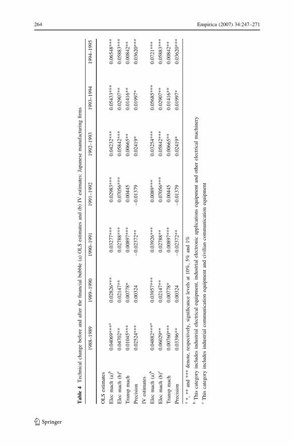
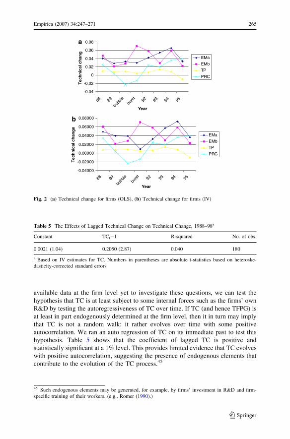
Table 4 shows, respectively, OLS and IV estimates for TC for firms in some

selected industries right before and after the burst of the Japanese financial bubble in

the late 1990. Figure 2a and b, respectively, show these OLS and IV estimates also.

We see from Table 4 and Fig. 2b that even the industries, electrical and

transportation machinery and precision industries, which are among Japan’s most

valued and highly efficient industries, experienced a significant drop in the rate of

TC in the few years prior to the bubble (1986–1989).44 The expansion of their

production facilities was not accompanied by TC. It was inevitable that these firms

were going to suffer from a significant amount of excess production capacity. This

over-investment situation was much worse in certain non-manufacturing sectors

(e.g., real estate development and construction sectors) than manufacturing sectors.

In fact the excess capacity which was caused by the excessive and misguided

investment in the late 1980s, along with the non-performing loans that financed it, is

still plaguing the Japanese economy.

One of the current policy issues of interest in Japan is to ascertain the degree to

which TC is determined by the forces exogenous to the firms. For example, how

much of firms’ TC can be created by the firms’ own efforts and how much is due to

outside factors such as the spillovers from other firms? While there are no publicly

43 This suggests that the type of variation we have is not correlated with the error terms of our estimating

equations.44 We observe essentially the same phenomena from the OLS estimates (Table 4 and Fig. 2a).

Empirica (2007) 34:247–271 263

123

Tab

le4

Tec

hn

ical

chan

ge

bef

ore

and

afte

rth

efi

nan

cial

bu

bble

(a)

OL

Ses

tim

ates

and

(b)

IVes

tim

ates

:Ja

pan

ese

man

ufa

ctu

rin

gfi

rms

19

88–

19

89

19

89–

19

90

19

90–

19

91

19

91–

19

92

19

92–

19

93

19

93–

19

94

19

94

–1

99

5

OL

Ses

tim

ates

Ele

cm

ach

(a)b

0.0

40

69

**

*a

0.0

28

26

**

*0

.032

77

**

*0

.029

83

**

*0

.042

32

**

*0

.054

33

**

*0

.06

54

8**

*

Ele

cm

ach

(b)c

0.0

47

02

**

0.0

21

47

**

0.0

27

88

**

*0

.070

56

**

*0

.058

42

**

*0

.029

07

**

0.0

58

83

**

*

Tra

nsp

mac

h0

.010

45

**

*0

.007

78

*0

.008

97

**

*0

.004

45

0.0

06

65

**

0.0

14

16

**

0.0

08

42

**

Pre

cisi

on

0.0

25

24

**

*0

.003

24

�0

.023

72

**

�0

.013

79

0.0

24

19

*0

.019

97

*0

.03

62

0**

*

IVes

tim

ates

Ele

cm

ach

(a)b

0.0

48

82

**

*a

0.0

39

57

**

*0

.039

26

**

*0

.008

9*

**

0.0

32

54

**

*0

.056

85

**

*0

.07

21

***

Ele

cm

ach

(b)c

0.0

60

29

**

0.0

21

47

**

0.0

27

88

**

0.0

70

56

**

*0

.058

42

**

*0

.029

07

**

0.0

58

83

**

*

Tra

nsp

mac

h0

.007

60

**

*0

.007

78

*0

.008

97

**

*0

.004

45

0.0

06

65

**

0.0

14

16

**

0.0

08

42

**

Pre

cisi

on

0.0

33

96

**

0.0

03

24

�0

.023

72

**

�0

.013

79

0.0

24

19

*0

.019

97

*0

.03

62

0**

*

a*

,*

*an

d*

**

den

ote

,re

spec

tiv

ely,

sig

nifi

can

cele

vel

sat

10

%,

5%

and

1%

bT

his

cate

gory

incl

udes

indust

rial

elec

tric

aleq

uip

men

t,in

dust

rial

elec

tronic

appli

cati

ons

equip

men

tan

doth

erel

ectr

ical

mac

hin

ery

cT

his

cate

gory

incl

udes

indust

rial

com

munic

atio

neq

uip

men

tan

dci

vil

ian

com

munic

atio

neq

uip

men

t

264 Empirica (2007) 34:247–271

123

available data at the firm level yet to investigate these questions, we can test the

hypothesis that TC is at least subject to some internal forces such as the firms’ own

R&D by testing the autoregressiveness of TC over time. If TC (and hence TFPG) is

at least in part endogenously determined at the firm level, then it in turn may imply

that TC is not a random walk: it rather evolves over time with some positive

autocorrelation. We ran an auto regression of TC on its immediate past to test this

hypothesis. Table 5 shows that the coefficient of lagged TC is positive and

statistically significant at a 1% level. This provides limited evidence that TC evolves

with positive autocorrelation, suggesting the presence of endogenous elements that

contribute to the evolution of the TC process.45

Table 5 The Effects of Lagged Technical Change on Technical Change, 1988–98a

Constant TCt�1 R-squared No. of obs.

0.0021 (1.04) 0.2050 (2.87) 0.040 180

a Based on IV estimates for TC. Numbers in parentheses are absolute t-statistics based on heteroske-

dasticity-corrected standard errors

-0.04

-0.02

0

0.02

0.04

0.06

0.08

88 98ubb

lb eb

tsru29 39 49 59

Year

a

gna

hclacin

h ceT

EMa

EMb

TP

PRC

-0.04000

-0.02000

0.00000

0.02000

0.04000

0.06000

0.08000

88 89

bbub el

ubrs

t92 93 94 95

Year

eg

nahclaci

nhce

T

EMa

EMb

TP

PRC

b

Fig. 2 (a) Technical change for firms (OLS), (b) Technical change for firms (IV)

45 Such endogenous elements may be generated, for example, by firms’ investment in R&D and firm-

specific training of their workers. (e.g., Romer (1990).)

Empirica (2007) 34:247–271 265

123

6 Concluding remarks

In this paper we have presented an econometric method based on index number

theory for estimating firms’ TC and returns to scale using panel data. Our paper is

a contribution to a substantial and growing literature on this methodological

problem.46 Then we have used the method to estimate TC, returns to scale and

total factor productivity growth for Japanese manufacturing firms for the period

1988–1998. We have discussed the movement of these estimated quantities over

time, particularly around the burst of the financial bubble in Japan. We have shown

that a significant decline in TC, and, to a lesser extent, a decline in total factor

productivity growth for many of the manufacturing industries was observed during

the period when the bubble was being formed but prior to the burst of the bubble.

This is consistent with the interpretation that massive investments in inputs were

made by Japanese manufacturers in the late 1980s to increase their output, while

such an expansion of the output was not accompanied by positive TC. This

resulted in the observed excess capacity for Japanese manufacturing firms. Many

Japanese manufacturers were suffering from excess capacity until recently. The

excess capacity was also the main cause of Japanese banks’ non-performing

loans.47

Another interesting finding of this paper is that the rate of TC in many Japanese

manufacturing industries did recover to the pre-bubble level in the post-bubble

period. This may explain why many parts of the Japanese manufacturing sector did

not collapse in the 1990s after the burst of the bubble, despite the negative post-

bubble circumstances and the lack of effective government and Bank of Japan

policies to move Japan’s economy out of the long-lasting recession. Some industries

have managed to maintain (or regain) a certain level of global competitiveness.48

One of the reasons for this may be the TC that continued to take place at the firm

level.

Acknowledgements Research in part supported by research grants from the Social Science andHumanities Research Council of Canada. We thank the editor and an anonymous referee for their helpfulcomments in revising the original version of the paper.

46 See, for example, Balk (1993, 1998, 2001), Diewert et al. (2006), Diewert and Fox (2004, 2005),

Diewert and Lawrence (2005), Diewert and Nakamura (2006), Grosskopf (2003), Fare et al. (1994), Hall

(1990), and Milana (2005).47 Excessive investment in other sectors such as real estate and property development during the bubble

period is another factor which has damaged the Japanese economy.48 For example, Japanese manufacturing industries ranging from what many regard as declining

industries (e.g., shipbuilding, steel) to traditionally competitive industries (e.g., auto, electronics) have

shown persistent resilience in their global competitiveness. Lau (2003), for example, cites as Japan’s

continuing comparative advantage the following: capital goods production, complex production processes

and R&D capability.

266 Empirica (2007) 34:247–271

123

Tab

leA

1D

escr

ipti

ve

stat

isti

csfo

rm

anufa

cturi

ng

firm

sin

sele

cted

indust

ries

a

Ele

cm

ach

(a)

Ele

cm

ach

(b)

Tra

nsp

mac

hP

reci

sio

n

Yea

rV

arM

ean

SD

Sm

plb

Mea

nS

DS

mp

lbM

ean

SD

Sm

plb

Mea

nS

DS

mp

lb

19

88–

19

89

ln(y

)1

0.7

31

.29

13

21

41

1.1

11

1.3

56

41

00

11

.27

61

.394

81

98

10

.53

51

.20

65

64

ln(Q

)0

.09

23

1.3

53

42

14

0.0

66

71

.352

91

00

0.1

13

11

.420

81

98

0.1

61

61

.31

23

64

D0

.52

14

0.5

10

00

.51

98

0.5

64

19

89–

19

90

ln(y

)1

0.8

64

1.2

84

92

28

11

.20

91

.394

61

08

11

.35

71

.398

82

14

10

.60

21

.20

41

66

ln(Q

)0

.10

85

1.3

28

22

28

0.1

16

71

.401

10

80

.111

61

.427

22

14

0.1

77

61

.30

71

66

D0

.52

28

0.5

10

80

.52

14

0.5

66

19

90–

19

91

ln(y

)1

0.9

23

1.2

93

62

30

11

.29

1.3

66

31

14

11

.34

21

.397

52

28

10

.69

91

.19

16

70

ln(Q

)0

.07

92

1.3

33

82

30

0.0

80

91

.402

51

14

0.0

85

61

.436

62

28

0.1

44

61

.28

98

70

D0

.52

30

0.5

11

40

.52

28

0.5

70

19

91–

19

92

ln(y

)1

0.9

15

1.2

95

92

32

11

.31

81

.373

21

16

11

.35

41

.408

62

26

10

.65

71

.24

04

68

ln(Q

)0

.01

83

1.3

48

62

32

0.0

15

61

.446

51

16

0.0

51

61

.446

92

26

0.0

47

21

.32

25

68

D0

.52

32

0.5

11

60

.52

26

0.5

68

19

92–

19

93

ln(y

)1

0.8

71

1.2

95

23

81

1.2

93

1.3

80

21

18

11

.30

31

.416

22

26

10

.57

91

.26

92

68

ln(Q

)0

.04

86

1.3

51

92

38

0.0

57

1.5

06

61

18

0.0

32

41

.457

52

26

0.0

69

41

.34

36

8

D0

.52

38

0.5

11

80

.52

26

0.5

68

19

93–

19

94

ln(y

)1

0.9

08

1.3

01

92

36

11

.37

81

.360

21

14

11

.17

1.3

18

92

18

10

.52

81

.24

88

72

ln(Q

)0

.08

21

1.3

66

92

36

0.1

10

51

.517

41

14

0.0

78

1.3

63

42

18

0.1

01

31

.31

87

72

D0

.52

36

0.5

11

40

.52

18

0.5

72

19

94–

19

95

ln(y

)1

0.9

77

1.3

09

82

40

11

.34

91

.354

31

14

11

.18

41

.284

92

20

10

.57

1.2

01

67

6

ln(Q

)0

.09

78

1.3

92

22

40

0.1

12

31

.519

21

14

0.0

61

61

.310

62

20

0.1

17

41

.27

81

76

D0

.52

40

0.5

11

40

.52

20

0.5

76

Ap

pen

dix

A.

Des

crip

tive

stati

stic

s

Empirica (2007) 34:247–271 267

123

Tab

leA

1co

nti

nu

ed

Ele

cm

ach

(a)

Ele

cm

ach

(b)

Tra

nsp

mac

hP

reci

sio

n

Yea

rV

arM

ean

SD

Sm

plb

Mea

nS

DS

mp

lbM

ean

SD

Sm

plb

Mea

nS

DS

mp

lb

19

95

–1

99

6ln

(y)

11

.11

71

.351

72

20

11

.37

91

.434

71

02

11

.31

1.3

99

52

20

10

.59

90

.987

27

0

ln(Q

)0

.083

11

.421

32

20

0.1

53

61

.590

71

02

0.0

89

61

.413

22

20

0.1

24

41

.069

57

0

D0

.52

20

0.5

10

20

.52

20

0.5

70

19

96

–1

99

7ln

(y)

11

.17

61

.371

21

81

1.4

69

1.4

80

11

06

11

.31

21

.411

92

20

10

.64

61

.010

27

0

ln(Q

)0

.078

31

.465

42

18

0.1

10

71

.637

10

60

.074

91

.419

92

20

0.1

12

11

.095

47

0

D0

.52

18

0.5

10

60

.52

20

0.5

70

19

97

–1

99

8ln

(y)

11

.13

41

.377

32

28

11

.44

71

.488

81

08

11

.25

61

.407

72

24

10

.61

21

.070

67

0

ln(Q

)0

.044

61

.476

12

28

0.0

86

71

.671

51

08

0.0

41

51

.405

42

24

0.0

77

71

.140

67

0

D0

.52

28

0.5

10

80

.52

24

0.5

70

aT

osa

ve

spac

ew

ep

rese

nt

des

crip

tiv

est

atis

tics

for

firm

sin

the

foll

ow

ing

man

ufa

ctu

rin

gin

du

stri

esin

this

tab

le:

elec

tric

mac

hin

ery

(a)

wh

ich

incl

ud

esin

du

stri

alel

ectr

ical

equip

men

t,in

dust

rial

elec

tronic

appli

cati

ons

equip

men

tan

doth

erel

ectr

ical

mac

hin

ery;

elec

tric

mac

hin

ery

(b)

whic

hin

cludes

indust

rial

com

mu

nic

atio

neq

uip

men

tan

d

civ

ilia

nco

mm

un

icat

ion

equ

ipm

ent;

tran

spo

rtat

ion

mac

hin

ery

and

pre

cisi

on

.D

escr

ipti

ve

stat

isti

csfo

ral

lm

anu

fact

uri

ng

ind

ust

ries

are

avai

lable

fro

mth

eau

tho

rso

nre

qu

est

bT

hes

esa

mp

lesi

zes

are

for

the

sam

ple

firm

sp

oo

led

ov

ertw

oco

nse

cuti

ve

yea

rsan

dh

ence

are

twic

eth

eac

tual

nu

mb

ero

fsa

mp

lefi

rms

inea

cho

fth

ein

du

stri

esin

the

giv

enti

me

per

iod.T

he

nu

mb

ers

of

man

ufa

ctu

rin

gfi

rms

for

the

ind

ust

ries

incl

ud

edin

ou

rst

ud

yfo

rth

e1

99

7–

199

8p

erio

dar

e:fo

od

(74

),p

ulp

(29

),p

rin

tin

g(1

9),

chem

ical

s

(15

1),

pla

stic

pro

du

cts

(28

),ru

bb

erp

rod

uct

s(1

6),

po

tter

yan

dce

ram

ics

(47

),st

eel

and

iro

n(4

7),

no

nfe

rro

us

met

als

(36

),m

etal

s(7

2),

gen

eral

mac

hin

ery

(a)

(65

),g

ener

al

mac

hin

ery

(b)

(10

8),

elec

tric

mac

hin

ery

(a)

(11

4),

elec

tric

mac

hin

ery

(b)

(54

),tr

ansp

ort

atio

nm

achin

ery

(11

2),

pre

cisi

on

(35

),te

xti

le(4

1)

and

pet

role

um

and

coal

pro

duct

s

(5).

Th

eto

tal

nu

mb

ero

ffi

rms

inth

esa

mp

leis

10

53.

Des

crip

tive

stat

isti

csfo

ral

lm

anu

fact

uri

ng

indu

stri

esfo

ral

lti

me

per

iods

are

avai

lab

lefr

om

the

auth

ors

on

req

ues

t

268 Empirica (2007) 34:247–271

123

7 Appendix B. Decomposition of TFP Growth

Table B1 Decomposition of average annual TFP growth at firms, 1988–1998

Industry TFP growtha Technical changeb Scale economiesb

Food 0.00329 0.00214 65 0.00115 35

Textile 0.01871 0.01585 85 0.00286 15

Pulp �0.00125 0.00163 �130 �0.00288 230

Printing �0.00738 �0.00677 92 �0.00061 8

Chemicals 0.00576 0.00762 132 �0.00186 �32

Petroleum/coal products �0.02151 �0.02625 122 0.00474 �22

Plastic products 0.01389 0.01141 82 0.00248 18

Rubber products 0.00792 0.00944 119 �0.00153 �19

Pottery 0.00102 0.00174 172 �0.00073 �71

Steel �0.00024 �0.00095 403 0.00072 �304

Non-ferrous metals �0.00334 �0.00500 150 0.00166 �50

Metal products �0.00786 �0.00509 65 �0.00278 35

General machinery(a)c �0.00044 0.00215 �494 �0.00259 594

General machinery(b)d �0.00097 0.00108 �111 �0.00205 211

Electrical machinery(a)e 0.02941 0.03489 119 �0.00549 �19

Electrical machinery (b)f 0.02767 0.03480 126 �0.00713 �26

Transportation machinery 0.00032 0.00046 144 �0.00014 �43

Precision �0.00016 0.00724 �4,522 �0.00740 4,622

a,b Numbers in the second of the two columns labeled ‘Technical change’ and ‘Scale economies,’

respectively, represent percentage contributionsc This category includes boilers, engines, metal processing machinery and general machinery partsd This category include general machinery which is not included in General Machinery (a)e This category includes industrial electrical equipment, industrial electronic applications equipment and

other electrical machineryf This category includes industrial communication equipment and civilian communication equipment

Table A2 Descriptive statistics: auto-regression of TCa

Variables sample Mean SD Min Max

TC 180 0.0027 0.0283 �0.1275 0.0811

TC(�1) 180 0.0032 0.0277 �0.1275 0.0811

Notes: IV estimates for TC which are available for firms in 18 industries were used in the auto-regression

of TC reported in Table 6. The sample used consists of 18 industries and 10 time periods

Empirica (2007) 34:247–271 269

123

References

Balk BM (1993) Malmquist productivity indexes and Fisher ideal indexes: comment. Econ J

103(418):680–682

Balk BM (1998) Industrial price, quantity, and productivity indices: the micro-economic theory and an

application. Kluwer Academic Publishers, Boston

Balk BM (2001) Scale Efficiency and Productivity Change. J Prod Anal 15:159–183

Banker RD, Charnes A, Cooper WW, Maindiratta A (1988) A comparison of DEA and translog estimates

of production frontiers using simulated observations from a known technology. In: Dogramaci A,

Fare R(eds) Applications of modern production theory: efficiency and productivity. Kluwer, New

York, pp 33–55

Burgess DF (1974) A cost minimization approach to import demand equations. Rev Econ Stat 56(2):224–

234

Caves R, Barton D (1990) Efficiency in U.S. manufacturing industries. MIT Press, MA

Caves DW, Christensen L, Diewert WE (1982) The economic theory of index numbers and the

measurement of input, output, and productivity. Econometrica 50(6):1393–1414

Chan NWL, Mountain DC (1983) Economies of Scale and the Tornqvist Discrete Measure of

Productivity Growth. Rev Econ Stat 70:663–667

Christensen LR, Jorgenson DW, Lau LJ (1971) Conjugate duality and the transcendental logarithmic

production function. Econometrica 39:255–256

Christensen LR, Jorgenson DW, Lau LJ (1973) Transcendental logarithmic production frontiers. Rev

Econ Stat 60:28–45

Diewert WE (1974) Applications of duality theory. In: Intrilligator MD, Kendrick DA (eds) Frontiers of

Quantitative Economics, vol II. North-Holland Publishing Co., Amsterdam, pp 106–171

Diewert WE (1976) Exact and superlative index numbers. J Econometrics 4(2):115–146, and reprinted as

Chapter 8 in Diewert and Nakamura (1993), 223–252

Diewert WE, Fox KJ (2004) On the estimation of returns to scale, technical progress and monopolistic

markups. Department of Economics, University of British Columbia, Discussion Paper, pp 04–09

Diewert WE, Fox KJ (2005) Malmquist and Tornqvist productivity indexes: returns to scale and technical

progress with imperfect competition. Center for Applied Economic Research Working Paper 2005/

03, University of New South Wales

Diewert WE, Lawrence D (2005) Australia’s productivity growth and the role of information and

communications technology: 1960–2004. Report prepared by Meyrick and Associates for the

Department of Communications, Information Technology and the Arts, Canberra

Diewert WE, Nakajima T, Nakamura A, Nakamura E, Nakamura M (2007) also referred to as DN4, The

Definition and estimation of returns to scale with an application to Japanese industries. In: Diewert

WE, Balk BM, Fixler D, Fox KJ, Nakamura AO (eds) Price and productivity measurement, Trafford

Press

Diewert WE, Nakamura AO (1993) Essays in index number theory, vol I. North-Holland, Amsterdam

Diewert WE, Nakamura AO (2007) The measurement of productivity for nations. In: Heckman JJ,

Leamer EE (eds) Handbook of Econometrics, vol 6. Elsevier Science (forthcoming)

Diewert WE (1999) Axiomatic and economic approaches to international comparisons. In: Heston A,

Lipsey RE (eds) International and interarea comparisons of income, output and prices. Studies in

Income and Wealth. vol 61. University of Chicago Press, Chicago, pp. 13–87

Fare R, Grosskopf S, Norris M, Zhang Z (1994) Productivity growth, technical progress, and efficiency

change in industrialized countries. Am Econ Rev 84:66–83

Fisher I (1922) The making of index numbers. Macmillan, New York

Godfrey LG (1988) Misspecification tests in econometrics: the lagrange multiplier principle and other

approaches. Econometric society monographs. Cambridge University Press, Cambridge, U.K

Grosskopf S (2003) Some remarks on productivity and its decompositions. J Prod Anal 20:459–474

Hall RE (1990) Invariance properties of Solow’s productivity residual. In: Diamond P (ed) Growth/

Productivity/Employment. MIT Press, pp. 71–112

Heckman JJ (1976) The common structure of statistical models of truncation, sample selection and

limited dependent variables. Annals of Economic and Social Measurement. December

Heckman JJ (1979) Sample selection bias as a specification error. Econometrica 47:153–161

Jorgenson DW, Nishimizu M (1978) U.S. and Japanese economic growth, 1952–1974: an international

comparison. Econ J 88: 707–726

270 Empirica (2007) 34:247–271

123

Kim JI, Lau LJ (1995) The sources of economic growth of the east Asian newly industrialized countries. J

Jpn Int Econ 8:235–271

Kuroda M, Kawai H, Shimpo K, Nomura K, Hikita K (2003) Structural change and productivity growth

in Japan: 1960–2000. Paper presented at the Rieti-Keio conference on the Japanese economy,

Tokyo, May

Lau L (2003) The impact of economic development of east Asia, including China, on Japan. Paper

presented at the Rieti-Keio conference on the Japanese Economy, Tokyo, May

Malmquist S (1953) Index numbers and indifference surfaces. Trabajos de Estadistica 4:209–242

Milana C (2005) The theory of exact and superlative index numbers revisited. EU KLEMS working paper

number 3

Morck R, Nakamura M (1999) Banks and corporate control in Japan. J Fin 54:319–339

Morck R, Nakamura M, Shivsasani A (2000) Banks, ownership structure, and firm value in Japan. J Bus

73:539–569

Nakajima T, Nakamura M, Yoshioka K (1998) An index number method for estimating scale economies

and technical change using time-series of cross-section data: sources of total factor productivity

growth for Japanese manufacturing, 1964–1988. Jpn Econ Rev 49:310–334

Nakajima T, Nakamura M, Yoshioka K (2001) Economic growth: past and present. In: Nakamura M (ed)

The Japanese business and economic system: history and prospects for the 21st century. Palgrave/

MacMillan/St.Martin’s Press, New York, pp 13–40

Nakamura A, Nakamura M (1981) On the relationships among several specification error tests presented

by Durbin, Wu and Hausman. Econometrica 49:1583–1588

Park S-R, Kwon JK (1995) Rapid economic growth with increasing returns to scale and little or no

productivity growth. Rev Econ Stat 77:332–351

OECD (2001) Measuring productivity: measurement of aggregate and industry-level productivity growth.

Organisation for Economic Co-operation and Development, Paris

Romer P (1990) Endogenous technological change. J Polit Econ 98:71–102

Theil H (1965) The information approach to demand analysis. Econometrica 33:288–293

Tornqvist L (1936) The bank of Finland’s consumption price index. Bank of Finland Monthly Bulletin

10:23–55

Tsurumi H, Wago H, Ilmakunnas P (1986) Gradual switching multivariate regression models with

stochastic cross-equational constraints and an appllication to the KLEM translog production model.

J Econ 31:235–253

Yoshioka K, Nakajima T, Nakamura M (1994) Sources of total factor productivity, Keio Economic

Observatory. Keio University, Tokyo

Empirica (2007) 34:247–271 271

123