technical efficiency in the indian textiles industry: a

University of ConnecticutOpenCommons@UConn

Economics Working Papers Department of Economics

November 2007

Technical Efficiency in the Indian Textiles Industry:A Nonparametric Analysis of Firm-Level DataAnup Kumar BhandariIndian Statistical Institute, Kolkata

Subhash C. RayUniversity of Connecticut

Follow this and additional works at: https://opencommons.uconn.edu/econ_wpapers

Recommended CitationBhandari, Anup Kumar and Ray, Subhash C., "Technical Efficiency in the Indian Textiles Industry: A Nonparametric Analysis of Firm-Level Data" (2007). Economics Working Papers. 200749.https://opencommons.uconn.edu/econ_wpapers/200749

http://lib.uconn.edu/?utm_source=opencommons.uconn.edu%2Fecon_wpapers%2F200749&utm_medium=PDF&utm_campaign=PDFCoverPages

http://lib.uconn.edu/?utm_source=opencommons.uconn.edu%2Fecon_wpapers%2F200749&utm_medium=PDF&utm_campaign=PDFCoverPages

https://opencommons.uconn.edu?utm_source=opencommons.uconn.edu%2Fecon_wpapers%2F200749&utm_medium=PDF&utm_campaign=PDFCoverPages

https://opencommons.uconn.edu/econ_wpapers?utm_source=opencommons.uconn.edu%2Fecon_wpapers%2F200749&utm_medium=PDF&utm_campaign=PDFCoverPages

https://opencommons.uconn.edu/econ?utm_source=opencommons.uconn.edu%2Fecon_wpapers%2F200749&utm_medium=PDF&utm_campaign=PDFCoverPages

https://opencommons.uconn.edu/econ_wpapers?utm_source=opencommons.uconn.edu%2Fecon_wpapers%2F200749&utm_medium=PDF&utm_campaign=PDFCoverPages

https://opencommons.uconn.edu/econ_wpapers/200749?utm_source=opencommons.uconn.edu%2Fecon_wpapers%2F200749&utm_medium=PDF&utm_campaign=PDFCoverPages

Department of Economics Working Paper Series

Technical Efficiency in the Indian Textiles Industry: A Nonpara-metric Analysis of Firm-Level Data

Anup Kumar BhandariIndian Statistical Institute, Kolkata

Subhash C. RayUniversity of Connecticut

Working Paper 2007-49

November 2007

341 Mansfield Road, Unit 1063Storrs, CT 06269–1063Phone: (860) 486–3022Fax: (860) 486–4463http://www.econ.uconn.edu/

This working paper is indexed on RePEc, http://repec.org/

AbstractThe Indian textiles industry is now at the crossroads with the phasing out of

quota regime that prevailed under the Multi-Fiber Agreement (MFA) until the endof 2004. In the face of a full integration of the textiles sector in the WTO, main-taining and enhancing productive efficiency is a precondition for competitivenessof the Indian firms in the new liberalized world market. In this paper we use dataobtained from the Annual Survey of Industries for a number ofyears to measurethe levels of technical efficiency in the Indian textiles industry at the firm level.We use both a grand frontier applicable to all firms and a groupfrontier specificto firms from any individual state, ownership, or organization type in order toevaluate their efficiencies. This permits us to separately identify how locational,proprietary, and organizational characteristics of a firm affect its performance.

Journal of Economic Literature Classification: L67, C61

Keywords: Data Envelopment Analysis; Meta-Frontier; Technology Close-ness ratio

2

TECHNICAL EFFICIENCY IN THE INDIAN TEXTILES INDUSTRY: A NONPARAMETRIC ANALYSIS OF FIRM-LEVEL DATA

Anup Kumar Bhandari Indian Statistical Institute, Kolkata, India

Subhash C. Ray University of Connecticut, Storrs, CT USA

Introduction

The Multi-Fiber Agreement (MFA) introduced in 1974 exempted international trade in

textiles and garments from the broad regulations of GATT and allowed countries to

impose bilateral quotas on import of various categories of textile products. Designed

primarily as a way to protect producers from the developed world against competition

from cheaper imports from the developing countries, the MFA has eventually been

phased out on January 1, 2005. This is a major change in the international trade scenario

for textile manufacturers across the world offering opportunities for penetration into

markets that have been off limits under the previous regime while at the same time

posing threats of market loss in the face of competition from other countries. For India, in

particular, performance of the textile industry in this new era can be of major significance

for the economy as a whole. In 2000-01 the textiles industry accounted for about 4% of

the GDP, 14% of industrial production, 18% of total industrial employment, and 27% of

export earnings1. Maintaining and enhancing productive efficiency is a precondition for

competitiveness in the new liberalized world market. India had bilateral arrangements

under MFA with the developed countries like USA, Canada, countries of the European

Union etc. Almost 70 per cent of India’s clothing exports have gone to the quota

countries of USA and the European communities. However, the Agreement on Textiles

and Clothing (ATC), 1995 of WTO envisages the dismantling of the MFA over a ten-

year period. Thus, after three decades textile industry has really been open to free

competition at the international level from 1st January 2005. The Indian textiles industry

is now at the crossroads with the phasing out of quota regime and the full integration of

the textiles sector in the WTO. Most of the studies undertaken to estimate the impact of

ATC expiry on textile trade share the finding that some Asian countries are most likely to

1 Hashim (2004)

3

benefit from the dismantling of the quotas. They predict a substantial increase in market

shares for China and India (see Government of India, 2004-05, pp. 144, for some

discussion on this issue).

India has a natural competitive advantage in terms of a strong and large multi-

fiber base and abundant cheap skilled labor. However, with prices being expected to fall

in the post-quota regime presumably owing to increased international trade and

competition, such an advantage may not be enough. Enhanced efficiency and

productivity are a must to meet this emerging challenge of global competition. It is

against this background that the performance of the Indian textile firms needs to be

examined rigorously.

In the pre-Reform decades numerous regulations enforced through rigid

bureaucratic control created a ‘permit-license Raj’ that effectively stunted productivity

growth and inhibited technical efficiency in Indian manufacturing. Various policies like

reservation of production of a large number of items for the small scale sector, high

customs tariffs distorting resource allocation and inhibiting the ability of Indian firms to

compete in the global markets, restrictions on capacity expansion restraining firms from

attaining efficient size, frictions faced in establishing and closing down of firms in

response to normal competitive market dynamics and various distortions created by the

structure of domestic trade taxes and excise duties discouraged efficiency and harmed

productivity growth. Introduction of various reforms and gradual liberalization of both

domestic and international trade marked the beginning of the end of the earlier regulatory

regime and a recognition of the urgency on the part of the Indian industries to become

efficient so as to be able to withstand successfully the pressure of foreign competition

(Government of India, 2000-01, pp. 149). Over the years several measures have been

taken by the government to help domestic industries achieve efficiency. These include

both financial measures such as rationalization of excise duties, liberalization of tax laws

and rates, reduction in interest rates and so on, as well as such physical measures as those

meant to remove infrastructural constraints in the power, transport and

telecommunications sectors.

So far as the structure of the textile industry is concerned, it continues to be

predominantly cotton-based with about 65 per cent of raw material consumed being

4

cotton. It has three sub-sectors – mills, power looms and handlooms. The latter two are

jointly considered under the heading ‘decentralized sector’. Over the years the

government has taken several steps to facilitate its growth. It has granted many

concessions and incentives to the decentralized sector with the result that the share of this

sector in total production has increased phenomenally. For example, while the share of

the mill sector in total fabric production was 76 per cent in 1950-51, it fell to 38 per cent

in 1980-81 and further to just 4 per cent in 2001-02. The share of the decentralized sector

rose correspondingly. In the decentralized sector, it is the power looms sub-sector that

has grown at a faster pace, producing as much as 76.8 per cent of the total fabric output

of this industry in 2001-02. The factors that have contributed to the fast development of

the power loom sector include government’s favorable policies on synthetic fabric

industry as well as the ability of this sub-sector to introduce flexibility in the product mix

in line with the market situation. In the mid-1980’s, a new textile policy was announced

to enable the industry to increase the supply of good quality cloth at reasonable prices for

both domestic consumption and export. In addition, a Textile Modernization Fund of INR

7.5 billion was created to meet the modernization requirements of this industry. In the

early 1990’s textile industry was de-licensed thereby abolishing the requirement of prior

government approval to set up textile units including power looms. A Technology

Upgradation Fund Scheme (TUFS) was also launched in 1999 to enable the textile units

to take up modernization projects, by providing an interest subsidy on borrowings.

The objective of this paper is to measure technical efficiency of Indian textile

firms for selected years using DEA. We also use the concept of a meta-frontier

production function introduced by Hayami (1969) and Hayami and Ruttan (1970, 1971)

to examine whether technology indeed varies among different locations, ownership

patterns, organizational patterns etc. of textile industry. Battese and Rao (2002) and

Battese, Rao and O’Donnell (2004) provide frameworks for such comparisons when

efficiency is measured using parametric stochastic frontier models. Rao, O’Donnell and

Battese (2003) provide both frameworks and an empirical application using FAO

agricultural data on 97 countries, comprise of about 99 per cent of both of global

agricultural production as well as world population. They provide framework for both

non-parametric DEA and parametric stochastic frontier methods as well. Das, Ray and

5

Nag (2007) use the concept of meta-frontier as a national or grand frontier in a

nonparametric study of branch level labor-use efficiency of a major public sector bank in

India.

In this paper we use firm level data from several different years of the Annual

Survey of Industries (ASI) for the Indian textiles industry. The annual cross section data

are used to construct a meta-frontier as well as separate group-specific frontiers for firms

classified by regional location, type of ownership and organization type. This permits us

to examine the proximity of any group frontier to the meta-frontier and measure such

proximity by what we define as the technology closeness ratio (TCR) of the group. Most

of the existing studies of productivity and efficiency in Indian manufacturing whether at

the level of total manufacturing (e.g., Ray (1997, 2002), Ray and Mukherjee (2005),

Mitra et al (2002), Krishna (2004)) or at the specific industry level (e.g., Trivedi (2004),

Hashim (2004)) use state-level data. Although Ram Mohan (2003) uses firm level data to

compare the performance of public and private sector firms, his data are constructed from

financial statements of companies and are not very accurate measures of input and output

quantities. This paper adds to the small number of studies that utilize input-output data at

the establishment level. Our approach provides a relative measure of overall efficiencies

of different groups (e.g., one state vis-à-vis another or public and private sector firms)

through a comparison of their technology closeness ratios (TCRs). At the same time, we

can evaluate the relative performance of individual firms within the constraints (like

infrastructure and work culture) faced by all firms within a group.

The paper is organized as follows. In Section 2 we describe the non-parametric

methodology of Data Envelopment Analysis (DEA) and explain the concept of a meta-

frontier as distinct from a group frontier. Section 3 gives some justification behind such

meta-frontier analysis to be considered for Indian industry and description of data and

variables considered for the production function is given in Section 4. Section 5

summarizes our empirical findings and Section 6 concludes.

2. The DEA Models

The non-parametric method of DEA introduced by Charnes, Cooper, and Rhodes

(1978) and further generalized by Banker, Charnes, and Cooper (1984) requires no

parametric specification of the production frontier. Using a sample of actually observed

6

input-output data and a number of fairly weak assumptions, it derives a benchmark output

quantity with which the actual output of a firm can be compared for (output-oriented)

efficiency measurement.

An input-output bundle (x, y) is feasible when the output bundle y (a nonnegative

vector of quantities of outputs) can be produced from the input bundle x (a nonnegative

vector of quantities of inputs). The set of all such feasible input-output bundles

constitutes the production possibility set T:

T = {(x, y): y can be produced from x; x ≥ 0; y ≥ 0} (1)

In the single output case, the frontier or the graph of the technology is defined by the

production function g(x) representing the maximum quantity of y that can be produced

using the input bundle x:

g(x) = maximum value of y, given x, where (x, y) ∈ T (2)

The corresponding production possibility set is: T = {(x, y): y ≤ g(x); x ≥ 0, y ≥ 0 }.

In the more general, multiple-output multiple-input, case, under the assumptions of

convexity of the production possibility set along with free disposability of both inputs

and outputs, the production possibility set can be empirically constructed as

( )

=∑ ∑ ≥=∑ ≤≥== ==

NjyyxxyxTN

j

N

jjj

jj

N

j

jj ...,,2,1;0;1;;:),(

11λλλλ (1a)

where ( jj yx , ) is the observed input-output bundle of an individual firm j in a sample of

N firms in the data.

The Group and Meta-Frontiers

Before one proceeds to construct the production frontier using the DEA in order

to measure the technical efficiency of a firm, it is necessary to recognize that all of the

observed firms may not have access to the same technology. Rather, different firms or

categories of firms may face different production technologies. A variety of geographical,

institutional, or other factors may give rise to such a situation. Constructing a single

production frontier based on all the data points would, in such cases, result in an

inappropriate benchmark technology. A way to measure the impact of technological

7

heterogeneity across groups is to construct a separate group frontier for each individual

group alongside a single grand or meta-frontier that applies to firms from all the groups.

In order to construct different production possibility sets for different groups, we

first group the observed input-output bundles by the locations of the corresponding firms.

Suppose N firms are observed and these firms are classified, according to some criterion,

into H number of distinct and exhaustive groups, thg group containing gN number of

firms

∑==

H

1ggNN . Define the index set of observations { }NJ ,...,2,1= and partition it

into non-overlapping subsets

{ })....,,2,1(;grouptobelongsfirm: HggjjJg == .

In this case, the production possibility set for group g will be

( )HgyyxxyxTJgj Jgj

gjgjj

gjJgj

jgj

g ...,,2,1};0;1;;:),( =

∑ ∑ ≥=∑ ≤≥=∈ ∈∈

λλλλ .

The set gT is the free disposal convex hull of the observed input-output bundles of firms

from group g. Suppose, that the observed input-output bundle of firm k in group g

is ).,( kg

kg yx A measure of the within-group (output-oriented) technical efficiency of the

firm k, is

kg

kgTE

ϕ1=

where kgϕ solves the following linear programming (LP) problem:

( )kgP =k

gϕ max ϕ

s. t. ∑ ≥∈ gJj

kg

jggj yy ;ϕλ

∑ ≤∈ gJj

kg

jggj xx ;λ ∑ =

∈ gJjgj ;1λ

ϕλ );,...,2,1(0 ggj Nj =≥ unrestricted.

The above LP problem is solved for each firm k in the thg group.

8

Next we consider the technical efficiency of the same firm k from group g

relative to a grand technological frontier, or what is called the meta-frontier. The meta-

frontier is the outer envelope of all of the group frontiers. It consists of the boundary

points of the free disposal convex hull of the input-output vector of all firms in the

sample. The (grand) technical efficiency of the firm k from group g is measured as

kG

kGTE

ϕ1=

where

=kGϕ max ϕ

s. t. ∑ ∑ ≥= ∈

H

g gJj

kg

jggj yy

1;ϕλ

∑ ∑ ≤= ∈

H

g gJj

kg

jggj xx

1;λ

∑ ∑ == ∈

H

g gJjgj

1;1λ

ϕλ );,...,2,1;,...,2,1(0 HgNj ggj ==≥ unrestricted.

In view of the fact that the grand production possibility set contains every group

production possibility set, it is obvious that kgϕ ≤ kGϕ and, hence, k

Gkg TETE ≥ , for every k

and g. In other words, firms cannot be more technically efficient when assessed against

the meta-frontier than when evaluated against a group frontier.

Technology Closeness Ratio

When, for any firm k in group g, the group efficiency and the grand efficiency measures

are close, we may argue that evaluated at the input bundle kgx , the relevant group frontier

is close to the meta-frontier. In stead of evaluating the proximity of the group frontier to

the meta-frontier at individual points, it is useful to get an overall measure of proximity

for the group as a whole. For this, we first define an average technical efficiency of the

firms in the group (i.e., relative to the group frontier) by the taking a geometric average

of such individual technical efficiencies. For the group g this will be given by

9

( ) gNgN

k

kgg TEgTE

/1

1

∏==

.

Similarly, the average technical efficiency of group g , measured from the meta-frontier,

will be

( ) ./1

1

gNgN

k

kGG TEgTE

∏==

For group g, an overall measure of proximity of the group frontier to the meta-frontier is

its technology closeness ratio

.)(

)()(

gTE

gTEgTCR

g

G=

TCR increases if the group frontier shifts towards the meta-frontier, ceteris paribus, and

is bounded above by unity which would be realized if and only if group frontier

coincides with the meta-frontier.

We illustrate these concepts in Figure 1 for the case of a single input – single

output – two groups of firms - group p and group q. Let the points P1 through P4 show

the input-output bundles of four firms from group p and Q1 through Q4 be the input-

output bundles of firms from group q. The group frontiers are shown by the broken line

AP1P3P4C for group p and by the broken line BQ1Q2Q3D for group q. By contrast, the

grand frontier is the outer envelop of the two frontiers shown by the broken line AP1P3

Q2Q3D. Note that the points within the triangle P3EQ2 lie above both the group frontiers,

but (by virtue of convexity) are within the grand frontier. While judged against their own

group frontier the technical efficiency of each of the points Q1, Q2, and Q3 equals unity

while the that of Q4 is .4 JKJQ When judged against the grand frontier or the meta-

frontier, TE of each of the points, Q2 and Q3, remains unity. However, the technical

efficiency of Q1 falls from unity to BNBQ1 , while that of the (inefficient) point Q4 is

the same as that with respect to its group frontier viz. JKJQ4 . Thus the average

technical efficiency of group q (measured from its group frontier) is given by, )(qTEq =

( ) 414 JKJQ and that (measured from the meta-frontier) is given by )(qTEG =

10

( )( )( ) ,4141 JKJQBNBQ which is obviously smaller than )(qTEq . The ratio of the two

measures the technology closeness ratio (TCR) of this group.

Figure 1. Group and Meta-Frontiers

3. Justification of Such Analysis in the Context of Indian Industry

India is a vast country with a number of states and union territories with their

distinct sociological, economic, political and infrastructural features. Easy access to

natural resources and other infrastructural facilities helpful in achieving lower cost per

unit of output is not evenly distributed all over the country. Sates differ widely in respect

of stability of government formed by different political parties, democratic nature of the

overall political environment, political and economic agenda of the political parties in

power, and the level of militancy of labor unions. Work culture of the people of the states

like Gujarat and Maharashtra is far more conducive to productive efficiency than what

one finds in states like West Bengal (Das et al, 2007). All these factors are important

determinants of the level of technical efficiency of a firm located in any particular region.

Although the core production function for different regions need not be different, these

environmental factors cause the underlying production function to shift away from the

global or meta-frontier. It is, therefore, proper to treat the production technology itself as

different for different regions of the country.

11

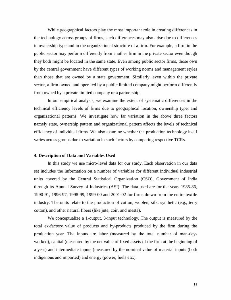
While geographical factors play the most important role in creating differences in

the technology across groups of firms, such differences may also arise due to differences

in ownership type and in the organizational structure of a firm. For example, a firm in the

public sector may perform differently from another firm in the private sector even though

they both might be located in the same state. Even among public sector firms, those own

by the central government have different types of working norms and management styles

than those that are owned by a state government. Similarly, even within the private

sector, a firm owned and operated by a public limited company might perform differently

from owned by a private limited company or a partnership.

In our empirical analysis, we examine the extent of systematic differences in the

technical efficiency levels of firms due to geographical location, ownership type, and

organizational patterns. We investigate how far variation in the above three factors

namely state, ownership pattern and organizational pattern affects the levels of technical

efficiency of individual firms. We also examine whether the production technology itself

varies across groups due to variation in such factors by comparing respective TCRs.

4. Description of Data and Variables Used

In this study we use micro-level data for our study. Each observation in our data

set includes the information on a number of variables for different individual industrial

units covered by the Central Statistical Organization (CSO), Government of India

through its Annual Survey of Industries (ASI). The data used are for the years 1985-86,

1990-91, 1996-97, 1998-99, 1999-00 and 2001-02 for firms drawn from the entire textile

industry. The units relate to the production of cotton, woolen, silk, synthetic (e.g., terry

cotton), and other natural fibers (like jute, coir, and mesta).

We conceptualize a 1-output, 3-input technology. The output is measured by the

total ex-factory value of products and by-products produced by the firm during the

production year. The inputs are labor (measured by the total number of man-days

worked), capital (measured by the net value of fixed assets of the firm at the beginning of

a year) and intermediate inputs (measured by the nominal value of material inputs (both

indigenous and imported) and energy (power, fuels etc.).

12

5. Empirical Findings

In order to perform meta-frontier analysis for studying the effects of difference in

location, we focus on six major textile-producing states namely Gujarat, Maharashtra,

Punjab, Rajasthan, Tamil Nadu and West Bengal. Observations from the rest of the

country contribute to the construction of the meta-frontier but are not analyzed as a single

group for measuring TCR. Similarly, we consider two types of ownership: private (i.e.,

wholly privately owned firms) and public (i.e., all of the remaining categories of firms

are combined into this group). Almost 90% of firms in the data set are under private

ownership in each of the years covered in the sample. Further, we consider six different

organization patterns: individual proprietorship (IP), partnership (Part), public limited

company (PULC), private limited company (PRLC), co-operative society (COOPS) and

the remaining are clubbed into ‘others’ category.

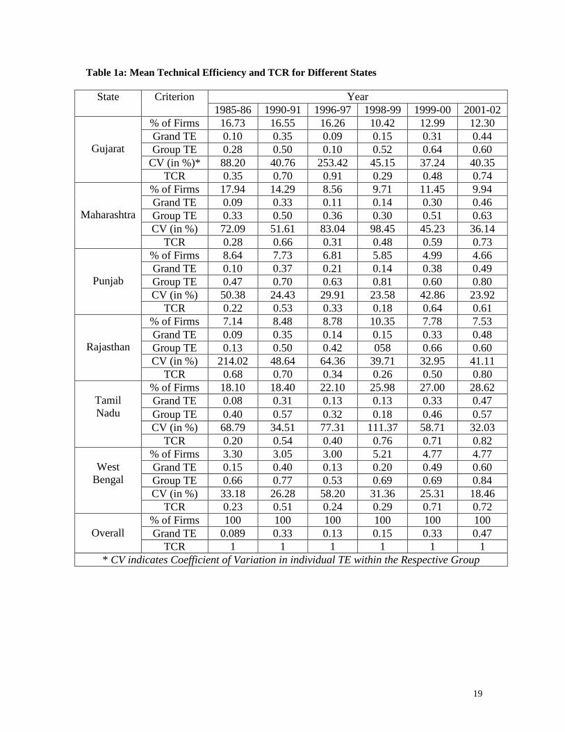
Average technical efficiency measured relative to either frontier as well as TCR

for different states are shown in Table 1a. In 5 out of the 6 years analyzed, West Bengal

had the highest level of average grand efficiency i.e., technical efficiency measured

relative to the meta-frontier. In the remaining year (1996-97) Punjab had the highest

grand efficiency. Two things need to be recognized in this context, however. First,

relatively few of the firms in the sample (between 3% and 5.21% in any given year) came

from West Bengal. Second, In 3 out of the 5 years, the average, although the highest for

the year across groups, was around 20%. Only in the last year (2001-02) did it reach a

respectable level of 60%. Hence, the West Bengal firms, although better generally than

others, are, nonetheless, quite inefficient overall.

Coming to the group efficiency i.e., technical efficiency measured against the

group frontier of each state, again West Bengal is found to be best performing with

averages ranging from 0.66 (in 1985-86) and 0.84 (in 2001-02). During the year 1996-97,

Punjab performed best relative to its state frontier with an average group efficiency score

of 0.63. Moreover, judging by the coefficient of variation (CV) in the year-wise group

efficiency levels, West Bengal (32.13%) and Punjab (32.51%) had the lowest yearly

average degrees of variability in technical efficiency across firms with the state. By

contrast, Gujarat (84.19%), Rajasthan (73.47%), Maharashtra (64.43%), and Tamilnadu

(63.79%) showed much greater variability in efficiency within the group. Thus, with

13

highest mean and lowest variability in the levels of efficiency, the West Bengal firms

appear to have performed in a superior fashion in most of the years.

A high level of TCR does not imply that firms in a specific state are, on an

average, more efficient. As explained in an earlier section, the TCR of any group is an

index of the proximity of the group frontier to the grand or meta-frontier over the

relevant range of variation in the input bundles. Bounded naturally between 0 and 1, a

high value of the TCR for any state implies that, on average, the maximum output

producible from an input bundle by a firm required to produce within the state would be

almost as high as what could be produced if the firm could choose to locate anywhere

else in the country. This, in its turn, implies only that there are no significant production

infrastructural constraints (e.g., physical, legal, cultural, etc.) that hinder productivity in

that state relative to the nation as a whole. This is best illustrated by the examples of

Gujarat in the year 1996-97 and West Bengal in 1985-86. In the case of Gujarat, in the

relevant year the TCR was as high as 91% showing that the group frontier for the state

was quite close to the grand frontier. However, relative to either frontier, the average

technical efficiency was particularly low – only 0.09 and 0.10. Thus, even though, the

state faced no particular disadvantage, the firms performed poorly. The case of West

Bengal was the opposite. The average level of group efficiency in 1985-86 was a

respectable 66%. But the grand efficiency was as low as 15%. The corresponding TCR of

0.23 shows that from an average input bundle a firm in West Bengal could at most

produce only 23% of what would be feasible elsewhere in India. The West Bengal firms

were doing reasonable well relative to a state benchmark but infrastructural constraints

hindered efficient production.

Another point to note is that for all states the TCR appears to have improved,

although not monotonically, over the years. This shows that in the post-Reform years,

market forces have been at work to remove the hurdles faced in the different states

bringing the state frontiers closer to the grand frontier.

Table 1b shows that except in the year 1985-86, levels of (grand) technical

efficiency of the private sector firms equal (in 1990-91) or exceed (in the other four

years) those of the public sector firms. In a parallel study using the stochastic frontier

approach, Bhandari and Maiti (2007) obtain similar results for the Indian textile industry.

14

Moreover, the grand frontier is supported primarily by firms from the private sector. This

is evident from the high levels of TCR for the private sector as a group and is especially

true in 1996-97 and the later years. The TCR of the public sector firms during this period,

although considerably lower than unity, has been improving. This suggests that, as group,

public sector firms have improved their productive potential in the more recent years.

As for organization type, public limited companies (identified as PULC in Table

1c) have higher (grand) technical efficiency as well as superior technology (as shown by

TCR) relative to all other organizational types of firms in our sample. This is broadly

consistent with the widely held belief that accountability of the corporate management to

the shareholders contributes to better performance.

It is evident from Tables 1a-1c that there are significant differences across groups

when firms are classified by any single criterion (region, ownership type, or organization

type) without controlling the other factors. But exclusive focus on a single criterion may

hide the consequences of variations in any other characteristic. For an example, it is not

obvious from Table 1a that the superior performance of West Bengal firms is due to their

location only. The partial effect of differences in any one category can be accurately

measured only within a multiple regression model incorporating all the relevant

explanatory variables.

Table 2 reports the estimated regressions for the different sample years using

yearly cross section data. The dependent variable is the measured level of (grand)

technical efficiency of an individual firm for the particular year. The dummy variables

Gujarat D through West Bengal D are the state dummies. The category “all other states”

is treated as the reference group. In the ownership classification, Public D is the dummy

variable for public sector firms with private ownership is the reference category. In the

organization type category, the dummy variables identify firms as individual

proprietorship (IP D), partnership (Partnership D), public limited companies (PULC D),

private limited companies (PRLC D), and cooperatives (Coops D). Firms of other

organization types constitute the reference group. Apart from the various categorical

variables, also included as regressors, are the size of a firm and its age. Size is measured

by the nominal value of its intermediate inputs. Age is measured in years. Because the

data set does not identify individual firms, it was not possible to estimate a panel

15

regression. In stead, annual cross section data were used to estimate separate regressions

for individual years. Of the 36 coefficients associated with the state dummy variables, 20

are significant at the 5% (or lower) levels. In general, their signs and magnitudes are

consistent with what one could derive from the difference of means for the individual

states in any year with the “catch all” group (identified as “all others” in Table 1a).

Nonetheless, further insights beyond what is obtained from Table 1a can be gained from

a careful perusal of the regressions reported in Table 2. For an example, consider the case

of West Bengal for the year 1990-91. In Table 1a, it has the highest average level of

(grand) technical efficiency exceeding the corresponding measure for overall by 0.07. In

the regression for the relevant year reported in Table 2, the coefficient of the West Bengal

dummy variable is only 0.016. Moreover, it is not even statistically significant! By

contrast, for the same year, the difference for Punjab is 0.04 in Table 1a and the

coefficient of the Punjab dummy variable in 1990-91 in Table 2 is a comparable 0.045.

This shows that controlling for other factors some times (though not always) could

portray a different picture about technological differences across states. As for the other

(non-categorical) variables, the coefficient of size (I), is uniformly positive and highly

significant. This implies that efficiency increases with firm size. By contrast, the

coefficient of age is significantly positive in the first two years but becomes statistically

insignificant thereafter.

The main findings of our empirical analysis can be summarized as follows.

• Firms from the state of West Bengal performed at higher average levels of technical

efficiency with respect to both their state frontier and a grand frontier applicable to

firms from all states.

• There were significant technological differences across states. However, firms from

states with more productive technologies often ended up performing at low levels of

efficiency as is evident from the case of Gujarat in the year 1990-91.

• There is some evidence that states with less productive technologies are gradually

catching up to the national benchmark.

• Private sector firms were more efficient than and also technologically superior to

firms from the public sector.

16

• Firms organized as public limited companies performed better than firms of other

organizational types.

• Technical efficiency tends to increase with firm size.

• Despite some initial evidence of positive impact, the age of a firm did not appear to

be significantly influencing technical efficiency in the later years in our sample.

6. Conclusion

In this paper we have measured the levels of technical efficiency of firms from the

Indian textiles industry in different years. Our study allows one to separately identify the

contribution of technological differences across groups of firms towards the overall

measure of technical efficiency. Superior performance of public limited companies in the

private sectors suggests that this should be encouraged as a preferred organizational form.

Also, consolidation of smaller firms into larger entities would enhance efficiency. Our

measures of technical efficiency suggest considerable room for increasing output without

requiring any additional inputs. Hence, even without an increase in allocative efficiency

through appropriately changing the input mix, average cost of production in the textiles

industry could be lowered significantly – often by 40% or more. This would greatly help

the competitive position of Indian firms in the world market.

References:

• Banker, R. D., A. Charnes, and W. W. Cooper (1984), “Some Models for Estimating

Technical and Scale Inefficiencies in Data Envelopment Analysis”, Management

Science, 30 (9), 1078-1092.

• Battese, G. E., and D. S. P. Rao (2002), “Technology Gap, Efficiency and a

Stochastic Meta-frontier Function”, International Journal of Business and

Economics, 1 (2), 87-93.

• Battese, G. E., D. S. P. Rao, and C. J. O’Donnell (2004), “A Meta-frontier Production

Function for Estimation of Technical Efficiencies and Technology Gaps for Firms

Operating Under Different Technologies”, Journal of Productivity Analysis, 21 (1),

91-103.

17

• Bhandari, A. K. and P. Maiti (2007), “Efficiency of Indian Manufacturing Firms:

Textile Industry as a Case Study”, International Journal of Business and Economics,

6 (1), 71-88.

• Charnes, A., W. W. Cooper, and E. Rhodes (1978), “Measuring the Efficiency of

Decision Making Units”, European Journal of Operational Research, 2 (6), 429-444.

• Das, A., S. C. Ray, and A. Nag (2007), “Labor-Use Efficiency in Indian Banking: A

Branch Level Analysis”, Omega, forthcoming.

• Government of India (2000-01), Economic Survey, Ministry of Finance.

• Government of India (2004-05), Economic Survey, Ministry of Finance.

• Hashim, D. A. (2004). “Cost and Productivity in Indian Textiles: Post MFA

Implications”, Working Paper No. 147, Indian Council for Research on International

Economic Relations, New Delhi.

• Hayami, Y. (1969), “Sources of Agricultural Productivity Gap among Selected

Countries”, American Journal of Agricultural Economics, 51 (3), 564-575.

• Hayami, Y., and V. W. Ruttan (1970), “Agricultural Productivity Differences among

Countries”, American Economic Review, 60 (5), 895-911.

• Hayami, Y., and V. W. Ruttan (1971), “Agricultural Development: An International

Perspective”, Johns Hopkins University Press, Baltimore, pp. 82.

• Krishna, K. L. (2004), “Patterns and Determinants of Economic Growth in Indian

States”, Working Paper No. 144, Indian Council for Research on International

Economic Relations, New Delhi.

• Mitra, A., A. Varoudakis, and M-A. Veganzones-Voroudakis (2002) “Productivity

and Technical Efficiency in Indian States’ Manufacturing: the role of Infrastructure”,

Economic Development and Cultural Change, 50 (2), 395-426.

• Ram Mohan, T. T. (2005) Privatisation in India: Challenging Economic Orthodoxy,

Taylor and Francis & Co.

• Rao, D. S. P., C. J. O'Donnell, and G. E. Battese (2003), “Meta-frontier Functions for

the Study of Inter-Regional Productivity Differences”, CEPA Working Papers Series,

WP012003, School of Economics, University of Queensland, Australia.

18

• Ray, S. C. (1997), “Regional Variation in Productivity Growth in Indian

Manufacturing: A Nonparametric Analysis”, Journal of Quantitative Economics, 13

(1), 73-94.

• Ray, S. C. (2002), “Did India’s Economic Reforms Improve Efficiency and

Productivity? A Nonparametric Analysis of the Initial Evidence from

Manufacturing”, Indian Economic Review, 37 (1), 23-57.

• Ray, S. C. (2004), “Data Envelopment Analysis: Theory and Techniques for

Economics and Operations Research”, Cambridge University Press.

• Ray, S. C., and K. Mukherjee (2005), “Does the Presence of Surplus Labor Hinder

Production in Indian Manufacturing?”, in S. Marjit and N. Banerjee (Eds.),

Development, Displacement, and Disparity: India in the Last Quarter of the Century,

Orient Longman.

• Trivedi, P. (2004), “An Inter-State Perspective on Manufacturing Productivity in

India: 1980-81 to 2000-01, Indian Economic Review, 39 (1), 203-237.

19

Table 1a: Mean Technical Efficiency and TCR for Different States

Year State Criterion 1985-86 1990-91 1996-97 1998-99 1999-00 2001-02

% of Firms 16.73 16.55 16.26 10.42 12.99 12.30 Grand TE 0.10 0.35 0.09 0.15 0.31 0.44 Group TE 0.28 0.50 0.10 0.52 0.64 0.60

CV (in %)* 88.20 40.76 253.42 45.15 37.24 40.35

Gujarat

TCR 0.35 0.70 0.91 0.29 0.48 0.74 % of Firms 17.94 14.29 8.56 9.71 11.45 9.94 Grand TE 0.09 0.33 0.11 0.14 0.30 0.46 Group TE 0.33 0.50 0.36 0.30 0.51 0.63 CV (in %) 72.09 51.61 83.04 98.45 45.23 36.14

Maharashtra


Punjab

TCR 0.22 0.53 0.33 0.18 0.64 0.61 % of Firms 7.14 8.48 8.78 10.35 7.78 7.53 Grand TE 0.09 0.35 0.14 0.15 0.33 0.48 Group TE 0.13 0.50 0.42 058 0.66 0.60 CV (in %) 214.02 48.64 64.36 39.71 32.95 41.11

Rajasthan


Tamil Nadu


West

Bengal

TCR 0.23 0.51 0.24 0.29 0.71 0.72 % of Firms 100 100 100 100 100 100 Grand TE 0.089 0.33 0.13 0.15 0.33 0.47

Overall

TCR 1 1 1 1 1 1 * CV indicates Coefficient of Variation in individual TE within the Respective Group

20

Table 1b: Mean Technical Efficiency and TCR for Ownership Variation

Year Ownership Criterion 1985-86 1990-91 1996-97 1998-99 1999-00 2001-02

% of Firms 11.67 12.19 11.26 16.20 14.89 10.93 Grand TE 0.11 0.33 0.09 0.11 0.28 0.39 Group TE 0.18 0.46 0.42 0.36 0.59 0.58 CV (in %) 133.76 62.48 70.04 69.18 41.83 39.34

Public


Private

TCR 0.79 0.921 0.993 0.996 0.999 0.998

21

Table 1c: Mean Technical Efficiency and TCR for Organizational Variation

Year Organization Criterion 1985-86 1990-91 1996-97 1998-99 1999-00 2001-02

% of Firms 14.84 15.35 10.89 7.14 6.97 5.11 Grand TE 0.06 0.26 0.18 0.15 0.22 0.47 Group TE 0.28 0.40 0.30 0.52 0.76 0.76 CV (in %) 93.50 64.35 98.06 40.34 23.21 24.26

IP


Part


PULC


PRLC


COOPS


Others

TCR 0.62 0.73 0.24 0.18 0.37 0.64

22

Table 2: Regression Results Explaining (Grand) Technical Efficiency Score using Different State, Ownership and Organization Dummies

Estimated Coefficient Independent Variable 1985-86 1990-91 1996-97 1998-99 1999-00 2001-02 Gujrat D 0.011** 0.022*** - 0.051*** - 0.002 - 0.028 - 0.035**

Maharashtra D 0.008 0.018** - 0.058*** - 0.017 - 0.007 - 0.012 Punjab D 0.015** 0.045*** 0.015 - 0.051*** 0.051** - 0.017

Rajasthan D 0.020*** 0.032*** - 0.042*** - 0.013 0.038* 0.001 Tamil Nadu D - 0.002 - 0.011* - 0.072*** - 0.033*** 0.003 - 0.022** West Bengal D 0.022** 0.016 - 0.024 0.050** 0.110*** 0.102***

Public D 0.035*** 0.015* - 0.069*** - 0.046*** - 0.035* - 0.071*** IP D - 0.033*** - 0.039*** 0.058*** 0.076*** - 0.012 0.057**

Partnership D - 0.007 - 0.007 0.033** 0.036* 0.033 0.047** PULC D 0.103*** 0.091*** - 0.029** 0.006 0.098*** 0.043** PRLC D 0.059*** 0.047*** - 0.056*** 0.014 0.050* 0.025 Coops D - 0.039*** - 0.059*** 0.010 0.008 0.012 0.028

( )810/I 0.152*** 0.071*** 0.019*** 0.022*** 0.018*** 0.014***

( )210/Age 0.058*** 0.082*** 0.007 0.008 - 0.036 0.015

Constant 0.094*** 0.320*** 0.238*** 0.155*** 0.308*** 0.465*** 2R (in %) 46.89 30.18 15.28 25.22 24.22 17.23

2R (in %) 46.75 29.97 14.95 24.46 23.44 16.55

*, ** and *** indicates significant at 10%, 5% and 1% respectively in a two-tailed test.

technical efficiency in the indian textiles industry: a

Documents