technical memorandums - nasa · technical memorandums-1 natioitaladvisory 601vu41$t!eeror...

TECHNICAL MEMORANDUMS-1

NAT IOITAL AD VIs ORy 601vu41$T!EEroR AERONAUTICS

,,. .

No. 1o58—--—— _—.—-

.

THE THIIIORY01’A FREE JET OF A COI~,PRESSIBLE GAS

T3y G. IT. Abram ovich

Central Aero–Hydrodynamical Institute

———————-—

- -. — - --- —-

V~ashingtGnMarch 1944

https://ntrs.nasa.gov/search.jsp?R=20050019538 2018-09-29T20:36:30+00:00Z

-.————

‘Illlllllllllllllmililll!mllllllllllllll~j 31176014415153 ;— _

NATIONAL ADVISORY COMMITTEE—------—

TECHNICAL MEMORANDUIVL,. .. ... ....

------- ——

THE THEORY OF A I?R~E JET OF “A

FOR AERONAUTIC S

NO. 1058---- ..- 1.

COMPRESSIBLE GAS*

By G. l?: Ab’ramovich ,.,...

SUMMARY .. .

In the present report the theory of free turbulencepropagation and the boundary layer ”theory are developedfor a plane-parallel free ‘stream of a compressible flui’doIn constructing the theory use was m’ade of the turbulencehypothesis by Taylor (transport of vorticity) which givesbest agreement with test ,results for yroblems involvingheat transfer in free jets.

The theory developed here considers two kinds of flow:. .

1. The boundary layer of a jet with temperaturedifferent from that of the surroundings and velocitiesthat are small by comparison with the veloc”ity of sound(Bairstow number Ba~ Oe5)o

2J. The boundary layer of a jet of high velocity andat a temperature equal to that of the surroundings.

The first deals with c,ompressihility effect arisingfrom the difference in temperatures inside and outside thejet; the second with the compr~ssibility effect arising fromthe high flow velocities.

The results indicated that the compressibility had”only a slight effect on the properties ?f the free jet.Furthermore it was found that a drop in,the. j-et..temperaturehad approximately the same ef’feet on the properties of thejet regardless of whether the reduc~ion was due to arti- -ficial cooling of the jet or to the conversion of thermalenergy to kinetic athigh flow velocities. -

Compressibility factors (~ and S) are introduced withthe aid of which it is possible to reduce the variations inall fundamental properties of the’ boundary lay~r ,under the

..,,_——_____— ________ ————.- .—__..-.___————————_—.— _______*Report No. 3’77, of the:Centra~ Aero_Hydrodynamical .Insti-tutel J,oscc)w, ~939e

,-. .“ ,. .

2 ,. NACA Technical M“emoratidum’No. 1058.

influence of compressibility-to sirn~le’linear relations.The results obtained are valltl ’”forflow velocities up tothe velocity of sound and for considerable temperaturedifferences (up to &100 - 150° C),

INTRODUCTION

In 1926 To~lmien$s paper was published (reference 1)in which the author, on the basis of the semi-empiricalgeneral turbulence theory of Prandtl, developed the theoryof so-called free turbulence — that is, turbulence in afree, heqted stream, In the same paper, making use of hisproposed theory, Tollmien solved three problems on thepropagation of free, heated jets:

(a) The boundary layer of an infinite plane-paralleljet:

(b) Plane-parallel jet escaping from a very narrowopening;

‘(c) ,Axially symmetric jet escaping from very narrowopening.

.

About 3 or 4 years later (1929–1930) Swainls paper(reference .2) and Schlichti’ng!s paper (reference 3) extend-ing the theory of free turbulence to the case of the wakelehind a body and developing the laws of flow in axiallysymmetric and ylane wakes appeared. These laws are appli-cable to flows not too near the body.

,.

The work’ of these authors was supplemented by experi–mental investigations of the velocity fields of flows Theuse of one empirical constant enabled the above-mentionedtheories to be brought into excellent agreement with testresults. In fact this agreement determined the succ?essof the Prandtl-Tollmien free-turbulence theory and assuredit wide theoretical and practical application. In 1935the article by Kuethe (reference 4) appeared in which anapproximate method is worked out for the computation of thevelocity profile in the initial part of a round jet.

In 1935, 1936, and 1938 four paper: by the presentauthor were published in which Tollmien!s t-heory was ex-tended to the case of plane-parallel flow and axiallysymmetric jets escaping fror, openings of finite diameter

q-— ---

NACA Technical Memorandum No- 1058 3

(an approxi~ate theory,of the initial part of the jet waspr+gpo~ed); f~rrn-ula~ were-worked out for the aerodynamiccommutation of the plane-par’til-l~”ljet’; axially symmetricjet flow in the o~en working part of a wind tunnel withround and elliptic sections, -hot and cold air jets, andmoreoverl xnethods were proposed for computing. the airresistance of railway cars (in tunnels or on the opentrack), pipe systems and heat interchangers (references~ 6, 7). These proposals and the flow theory itselfw~re satisfactorily confirmed by test results and eachyear find wide application to engineering practice.

“The rapid development of the mechanics of turbulentflow has prompted the application of the physical modelof the phenomena as conoeived by Prandtl and Tollmien tothe solution of heat problems, those of the temperaturedistribution along the jet axis and over its cross-sectionsof heat diffusion from the jet to the surrounding space,and so forth. It is interesting to note that as a directconsequence of the Prandtl theory, in the case of a freejet and the wake behind a body, complete similarity isobtained between the temperature and velocity fields. Iitorder to check this extremely important result rage andFalkner (reference 8), in 1932, made measurements of thevelocity and temperature fields in the wake behind a longcylinder of elliptic cross section, They showed that thetheoretical velocity fields of Prandtl—Schlichting werevery well confirmed by test results while there was nosimilarity of the velocity and temperature fields, andthe heat transfer from the wake to the undisturbed flowis of greater intensity than follows from the ?randtltheory, t

Taylor (reference 9) was the first to note the con-tradiction revealed in the free turbulence theory of Prandtland presented a hypothesis according to which the tangentialturbulent stresses in the flow were to be determined by thetransverse transport of vorticity and not by the momentumas proposed by Prandtla The imperfection in the Prandtltheory was also pointed out in that it took no account ofthe local pressure gradients which have an ap.preciahleeffect on the momentum interchange but not on the, vorticity,tqan.sporte The ap.oye h~.pothesis, with regard to the tur-bulence, was first proposed as far back as 1915 (referencelo)* On the basis of this hypothesis using only one em-pirical constant, as prandtl did, Taylor obtained the vel–ocity and temperature profiles in the wake behind a longcylinder as experimentally determined by rage and Falkner,

.

4., ‘-NA.CA Technical Memorandum Nb, 1058

The Taylor theory of free turbulence gave velocity pro-files accurately, the same as those given’by the Prandtltheory, and at the sa~e time removed the imperfection ofthe latter theory as regards application to heat problems.This,permits all the solutions ’of the problems in the fieldof flow meehafiics that were based on the Prandtl theory toretain their validity, It made it necessary, however, togive preference to the Taylor theory for the further devel–opment of the problems of free flow and the wake behind abody, particularly in ‘those cases when the problems areconcerned with temperature profiles and heat transfer.

In the present -peport devoted to the further develop-ment of the theory of the free jet, a theory of free turbu-lence in a compressible gas is worked out and so~utions aregiven of boundary layer problems of a free flow for thefollowing two cases;

(a) The loundary layer of a plane-parallel jet atsmall flow velocities with a temperature different fromthat of the surroundings, that is, a nonisothermal layer;

(b) Isothermal boundary layer at large (up to Bao=l)flow velocities.

It may be noted in conclusion that the free turbulenceproblems, in addition to being of interest in themselves,also possess a general interest since free turbulence repre-sents ,the simplest case of turbulence free from the effectof viscosity. The study of free turbillence is a necessarypreliminary stage in the study of turbulent flows in general.It is, therefore, hoped by the author that the solut.icn pro-posed in his present paper of the problems of free turbulencein a compressible gas possesses a certain usefulness for thest,udy of “turbulence” in other cases of compressible flow.

10 EQUATION OP NOTION FOR TREE TURBULENCE

The problem will be restricted to two-dimensional flow,In this case the differential equation of motion in the di-rection of the axis of abscissas assumes the following form:

—

NACA Technical Memorandum No.. 1058 5

where,,..>-----.“....- .

u, v instantaneous velocity components- ..

P9 PO k instantaneous values of “the density, pressure,and viscosity

For the flow of a liquid of small viscosity aboutsolid bodies the flow, as was shawn hy 2randtl as farback as 1904, may be divided into two regions; namely,a relatively thin layer of fluid lying close to the solidwalls — the boundary layer - in which .the.effect of theviscosity cannot be neglected, however small its valuemay be, and the remaining part of the flow, in which the,vi$cosity plays no part and’which is therefore su%jectto the laws of flow of ideal fluids, The boundary layer,in turn, is assumed to consist of a very thin sublayerof purely laminar flow in direct contact with the wall(no transverse turbulent fluctuations can be developedsince they are dissipated by the wall) and a remainingturbulent portion of the boundary layer in which theeffect of the viscosity may be neglected- Thus thestudy of the flow about solid bodies, the motion throughpipes and, in general, of all fluid flows in the presenceof rigid boundaries does not, in principle, permit neglect-ing entirely the effect of the viscosity This circum-stance constitutes the great obstacle in the developmentof the theory of turbulent flows,

The distinguishing property of free turbulent jetsis the absence of rigid flow boundaries and hence of alaminar suhlayer; This makes it possible to neglectentirely the effect of viscosity in all cases of freeturbulence and explains the dynamic similarity of thejet flows - the nondependence on the Reynolds number -over a very wide range of Reynolds number,

The differential equation of motion for two-dimensionalfree turbulence may thus be written in the following form:

. . . 0 . ..- ...- ... ,. i. ..., ~.

Due to the quasi–stationary state of the turbulentall its characteristics may be broken up into meanfluctuating components: \

(2)

motionand

.

6 NAOA !Cechnical-’-Memor~ndum “No”.‘-1058

‘! “~..

u= u+u~. .(.,------. . . . .... ,.&,,,.! .... .-. . .. .. ..

v= 7 +, Vf....- , ,.,. . ....-,’.1 (2a).:,:....’-

P= ~+ f)l”.-...,- ,. ,,-,,.,“. .,... -,‘.”G,

.. ,,,. P= T+P~ ,,. ..“ ,. .,,:..”:.. :’: .,.- -’1‘

On the averager’:ove~ ,8,certain finite tfm.e‘itite’rval,the

fluctuating comp.memt Ls,.evident.1$ equal..to’ zero: ‘.,,. -b.,.--- ,, t.~ -1 :,,... --.

,.-.,~.-. .....,, .’-, ,._ . -.-J‘ ,.,. >.----,.,.: .,....-. ‘:V1 =.Ul,= >~1p? ‘ ~.

..~:. ,..” .,.’. ,(2:)

,, .,!z.- ..-/. :4 .. . ,..!

. . .:- .,, .. .,.. . r..

In the-gener”al ca~e, however, this i’s not true if t.lie:,squares ‘of t-he “fluctuations and their’ products.’ - ‘..

,. ,, ,-, . .,,.+..’. . . . -’..

In equati~n (2) the mean values and fluctuations aresubstitut~d for, t-Kc instantaneous magnit-udes. To averageovz<r the ti’me, take account of. condition’s (e,quati”on(~b))and neglect mom-ents of’ th:e‘th’ird order.: , ‘

. . -., ,’-. I .,..

. .,., .there ‘i-s:?btai’ned the ‘differential equat,ion <or the a~srageturbu’leilt flow of a compressible fluid”:’ , ,.

.. ,.

‘ To estimate the order of magnitude of the individualterms that enter the above equation it is not difficult tosee that in the case of free turbulence ,all terms in thesecond bra,ck”ets (vith- ~eriv.ativ-es im.-re”s~”~ctto-x), “are’‘verysmall ‘by con-paris-on wi.t’h”the ‘~orre.sp.on~ing t-erms of thethird brackets (with derivatives ln”res~bct”to y) if the

NACA Technical Memorandum’ No’c 1058 7

~pincipal direction o.f.t&e f.l$w coincides with the axisof abscissas. Similarly one of t~~=terms of the thirdbrackets

. .

is negligibly small, By neglecting the above small termsthe following form of the differential equation of motionfor the case of two-dimensional purely turbulent flow is:

I?ree jets propagated in infinite space filled withliquid at rest, and wakes behind a body surrounded byinfinite undisturbed flow, possess such small pressuregradients that they may be neglected, With this in mindthe differential equation of motion for free turbulenceiil a compressible gas is:

-——___—__ —____—_—

--a; ––– aiipu=+pv=+v! [75*J+P’:;]=O (4)

L dy

The further steps in the solutiona

of the ’problem dependon the choice of physical model for the turbulent flow.At the present time there are two models of interest intheir application to free turbulence, namely, those ofPrandtl and Taylor. With the aid of the Prandtl modelresults agreeing with experin.ent are obtained for problemsin the field of jet mechanics (velocity fields, frictionalstress, and so forth) but strong disagreement is obtainedfor heat problem solutions, (temperature field, heat trans-”fer)s The Taylor physical model gives the same solutionsas the Prandtl model for the mechanical problems and further-more leads to solutions of the heat problems that are ingood agreement with e,xperiments,,c In what follows, there-fore, use is made of the Taylor model,- Tli’e’l’Zitt-e”ris basedon the assumption that the turbulent tangential stresses inthe flow arise from the transverse transport of vorticity,that is, from the correl~.tion between the vortex fluctuationsand the transverse velocity components. In two-dimensionalflow directed along the axis of abscissas the vorticity isgiven by

Ilm1111111-mm-

,, .,... ______ .

8 NAC~ Technical ~iemorandum No. 1058

(4a)

where the magnitude of h7/ ax in free turbulence isnegligibly small by comparison with hil/by so that

I aiiG= ---2 hy (=4b)

In its transverse transport, immediately before the lossof its individuality, the particle encounters a layer wherethe value of the vorticity differs from that in the layerfrom which it arrived by the amount

where IT is the mean free path of the fluid particlein the turbulent flows The loss of individuality of thefluid particle should be accompanied by a discontinuouschange (fluctuation) of vorticity of amount,,

BFrom equation (4b) it is clear, however, that

1 but~1.__2 by

hence

(4C)

With the loss of individuality of a given particle thereare naturally associated fluctuations of the flow velocity:

— ..

,NACA Technical Memorandum Noe 1058

and of ‘the fluid density: ‘ “ ..,. —-. ,.. ,., ;..;-?.>,, .-. s-. . ..!.... ‘- 4.,

apP’ ‘~T—

‘by ,(4e)

By making use of equations (4c) and (4e) equation (4) wasreduced to the form

,, ,. ,,,. . ,... . .,. .

——_—4’--b%p : + tiii

+ ;-7LU+‘r lT P’--–+----1

= o (5)by L bya by by

or

(6)

which is the differential equation obtained on the basis‘of the Taylor turbulence acdel. ,,

—-—.—With r~spect to the nagnitude Vt IT it is necessary

to make some assumptions by which it is associated with thevelocity of motion and with the coordinates of the systeLl_It is possible, for exanp~e, to make use of the generallyaccepted idea of Prandtl, nanely, that the transversevelocity fluctuations are of the same order of magnitudeas the longitudinal fluctuations:

. . ,,V!-’tit ,’

that ‘is,. .

(6a)

Including the proportionality constant i,n the magnitude ofthe free path of the par,ticle – the mixing, length (IT) -(equation (6)) is reduced to t,hemores imple, form*

(7)

.-———_ —_—_— ____________________ ______________________ ____*with, a view toward simplicity of notation the averaging barsovel” the letters are omitted in what follows so that p,T _and IT

2’—~ are *O stand for their mean values in time (p,u, v, and TT).

11 In ,,,.I ,,, ,, ,, ,,,,, , , ., , ,,,, I

10 NACA Technical Memorandum No. 1058

In the special case of an incompressible fluid (p =constant) the following is obtained

au+vauu—

a au a2u.~T —.=ax 7Y bY ay

(7a)

The corresponding equation derived from the turbulencemodel of Prandtl for the free turbulence in an incompress—ille fluid was obtained by Tollmien in 1926 in the follow-ing form (reference 1):

(7b)

TO take into account the fact that the constant of pr%portionality is determined from experir,ental data, it isseen that in the case of free turbulence the I?randtl andTaylor models give rise to the same equation of motionc

The value of the m~xing lengths, as given by Prandtland Taylor respectively, differ by the constant magnitude

“

-—

(7C)

For the purpose of’retaining the form of computation adoptedhy T!ollmien and others the Prandtl value of the mixinglength is assumed. The differential equation of motion forfree turbulence in a compressible gas then becomes

P“ ;;~aua [1+Pv~” = 21 — — P ~:ay ay ay i3Y

(8)

Comparison of the above equation with the generally knownequation for stationary flow

au a7xxPu=+pv:u=

bY ay(8a)

reveals the presence of “apparent” tangential stressesthe magnitude of which is given by the equation

—.—— —

‘NACA Technical Memorandum No, 1658

! aaub[]

?lU~xy = 21 —— dy

by by .P TY(8b)

In the case of an incompressible fluid equation (8b) re-duces to the, generally famili&r Prandtl law of turbulentfriction:

(8c)

.,

To solve equation (8) it is necessary to know a relationbetween the mixing length I and the coordinates of thesystem, The absence ‘in the case of free flow, of rigidboundaries that damp the fluctuating motions of the par-ticles led Prandtl to the assumption of constancy of themixing length in the transverse direction of flow:

l(Y) = constqnt (9)

It thus remains to estzblish the law of variation of themixing length along the axis of abscissas:

1 = l(x)

The available experimental investigations of free flows makeit possible without any particular difficulty to determinethe form of the fuilction 1(X)* A sufficient basis for thisis‘the experimentally established fact of similarity of theboundary layers in various cross sections of a given freeflow (jets or wakes, reference 1)- This similarity wasrevealed in a large number of experimental papers (Tollmien,l?~rthmann, Ruden, Schlichting, and others) by constructingvelocity profiles in nondimensional coordinates, for example,ii the form of the relation

. u-— = ofvUm ;

(9a)

.,

12

where

u

u=

b

NACA Technical Memorandum Noa 1058

velocity at a point with ordinate y

velocity on the axis of the jet .

width of the jet (or of its loundary layer);in thegiven cross section

The nondimensional velocity profiles (equation) werefoufld to agree for the various cross sections,

The similarity of the boundary layers at any twocross-sections of a given free flow must also be obtainedwith regard to geometric factors, In other words equalityis to be expected between the nondimensional mixing lengthsfor the various flow cross sections:

(9b)

It is thus sufficient to establish the law of increase ofwidth of jet along the axis of abscissas in order that thelaw of increase of the mixing length be known. A veryinteresting consideration of Prandtl permits the solutionof the relation b = b(x). It is shown by Prandtl (refer-ence 11) that the widening of the jet (or of the boundarylayer of the jet) arises from the transverse velocityfluctuations VI, that is,

( 10a)

Because of the similarity of the velocity profiles at tkiedifferent jet cross–sections the following equation may bewritten

au Um-..—by b

and further

(lOb)

NACA Technical Memorandum No. 1058 13

On the other handa the rate of expansion of the jet,.

.-

db db dx=—— , (1OC)z dx dt

that is,

db ~ db-— = urn-—dt dx

)

Comparison of expressions (lOb) and (1OC) leads to thesolution of the problem of the law of increase in widthof the free jet and of the mixing length in the flowdirection:

Q . constant -)dx !

The l>w oh.tained foralong the flow

1(11)

b = x constant

I=cx

the increase in the mixing length

1 =Cx (12a)

is valid for free jets of various shapes:, $or the boundarylayer of an infinite two—dimensional flows for a plane-parallel stream, axially symmetric stream and, in .genera.1,for those cases of free streams for which the flow profilesare similar. In the same manner, as previously described,the law of variation of the mixing length in a plane–parallel wake, axially symmetric wakes and so forth, maybe obtained- In the present paper$ which is devoted tothe free jet only, no consideration will be given to wakes.By making use of the relation oltained for the mixinglength along the jet the differential equation for freeturbulence in a compressible fluid is reduced to the newform

— —

14 NACA Technical Mesnorandurn No, 1058

This is the general equation satisfy~nfj anY case of afree jet of a compressible gas- The uagpitude c is

the only empirical constant in the theory of free tur-bulence, In the special case of an incompressible fluidequation (12) assumes the familiar f~rm given in Tollmienlspaper:

au aul.l—

ax+v~= 2C2X2

II* DIFFERENTIAL EQUATION OF

LAY13R IN A I?RIUIJXT Ol?A

(12b)

THE TURBULENT BOUNDARY

COMPRESSIBLE GAS

(PLANE-PARALLEL PROBLEM)

Assume a plane-parallel flow of compressible gasextending to infinity in OY direction (fig. 1) withundisturbed velocity Uo $ density Po, and startingfrom the point O, mix with the surrounding gas at rest,In accord with the law previously derived of the linearincrease in the width of the boundary layer 3 togetherwith the condition of similarity of velocity profilesthe velocity along any line C@ drawn from the originof coordinates O (the latter coincided with the pointwhere the boundary layer thickness b = O) remains con-stant as will be showna From the similarity of thevelocity profiles it follows that the velocity at corre-sponding points of the flow are equal, that is, for

there is

‘Ul ‘J2 ‘3= —— = —— = ● . ,=

~constant

‘o ‘o

But from equation (11)

3 = x constant

hence for

l?ACA Technical Memorandum Xo. 1058 15. . . .

.’

., ------ -- ...y/x ,= con~ta.nt.,. . .. . . (l$a)

there is the condition ‘

,, ‘u+= constant (13b)u’. .. 0,

f,>,

w!lich”proves what wad requlre~, s’ince equation (13a) isthe equation of a straight line through O, Thus in theturbulent boundary layer of a free flow the ,rays froma correspondingly chosen origin of coordinates areffisotachs. ”

The result obtained indicates that if the problemof the free plane boundary layer is solved in coordinatesx and q = yjx the velocity will depend cmly on m:

u= Uof(n) (14)

In order to eliminate the empirical constant from equation(12) the following equation is set

2C2 = a3 (15a)

and the following system of coordinates is chosen

Yx: Cf = --

., ax(15b)

Then

u= Uof((p) (15a)

There is introduced, as is usually done for compressibleflow cases$ the stream function for the product of themean velocity by the mean density and there is obtained

..,,

( 15d)

16 NACA Technical memorandum No. 1058

The density of the fluid in the case of free turbulence,for which the pressure gradients may be neglected, de–pends only on the temperatures

The temperature fields in free flows, as shown bythe tests of Fage and Falkner, Ruden, Olsen, and others,are similar as the velocity fieldse Otherwise expressed,the investigations of the temperatures show that in thefree boundary layer the isother~s, like the isotachs arestraight lines from the origin. Thus the temperatures,and hence also the densities, depend only on the non-dimensional coordinates (q):

t = to e(cp)~( (16)

P = Po K(V) J

On the basis of the foregoing a certain function F(cP),the first derivative of which is equal to the principalcomponent of the momentum, is introduced

Pu= p. U. 31 (17a)

where Po and Uo are the density and velocity, respec—tively, in undisturbed flow,

Hence

$= Jpudy = Po Uo ax J ~’dv

that is, the formula for the stream function is

Q= axpouoF

and for the transverse momentum:

(1’7b)

●

N.AGA Technical’ Memur’andu’m‘No. 1058 17

or

Substituting expressions (16), (1’7a), and (1’7c) inthe flifferential equation (12) and making certain elementarytransformations of the latter, using the expressions

(17d)

the ciifferential equation of the turbulent boundary layerin a plane-parallel free flow of a compressible gas inthe form is

At ail points of thz bou?:d~ry layer except its outer (6?2)anj- inner (wl) boundaries the derivative of the velocityis not equal to zero, that is,

Therefore the following is o“otained

L _!

and further

Thus the differential equation of the turbulent boundarylayer assumes the following form

.-. . .-——.


Frll = b

11

‘K’-F+-&v TF’

To solve the above equation it is necessary to know thedensity functiOn K = ~(q).

In the case of an incompressible fluid for whichK(q) = constant = 1 and K! = bK/bq = O equation (20)redu’ces to the well-known Tollmien equation:

corresponding to the case of the turbulent boundary layerin a free plane—parallel flow of an incompressible gas.

In what follows equation (20) corresponding to thecompressible gas will be solved for two cases:

1, l?ree flow at small velocities (up to Ba ~ 0-5)wit!l a temperature differing from that of the surroundingspace, that is, a nonisothermal flow,

2. Isothermal flow at large velocities (up to Ba = 1).

111. BOUNDARY LAYER OF NONISOTHERMAL PLANE-PAR.4LLEL JXT “

Ol? COMPRESSIBLE GAS AT LODERATE I’~OW Vi?LOCITIES

10 Heat Balance in the Turbulent Stream

In the present section the flow of a compressiblefluid (gas) in the boundary layer of a plane-parallelstream at moderate velocities but at temperatures differ—in: frc~, those of the surrounding fluid at rest shall beconsidered. In the later sections it will be shown thatthe effect of the compressibility of the gas arising fromthe high flow velocities is not large. Up to values ofthe llairstow number of the order Ba = 0-5 - 0.6 theeffect of the compressibility is barely appreciable. Forthis reason the equations and results which will be ob-tained in the present section devoted to the nonisothermaljet of small velocity w-ill maintain their validity up to

NACA Technical Memor-andum i~o.‘-1058 19

velocities of the order of 0.5.- 0.6 of the velocityof s@un&O ,..

..

To obtain the law of temperature distribution inthe boundary layer of a free jet use is made of thedifferential equation. of ““heatbalance, ;~herein themolecular heat conducti’on.and the coriversi”on of theenergy of the vi’scous forces into heat is neglectedwith respect to the turlmlent heat transfer in thesame manner as the frictian due to the v%scosity in thedynamic equation (2) was disregarded w.i.th respect tothe turbulent friction. Then “ . .

aT ?)T ?)T+ Pv -- = o‘X+pux ?)37

(21)

where

T temperature of the fluid

t time, seconds

It is Conveni.::n: ttj brea}: Up all the characteristicsof the turbulent fl,o-.v~.il.to their mean values and fluctu-ations about the mean values:

u= Ti+ut, v= T+vt, p =;+pt, T=~+TJ (22a)

so that on the average for a finite time interval thefluctuating components are reduced to zero:

v! = ;-7 . ;7 . ~-i= o,. . . .

Averaging with respect to time, while taking account ofequations (22a) and (22b) and neglecting moments of thethi,rd order:

(~TI

! UI _.._;~T 1 \,

P.,,- -ax ,P’v’ -;y)

equation (21) is transformed into the differential equa—tion Of heat balance for the turbulent quasi-stationary

6-? = ‘) ‘10’47: ~

20 NA(jA Technical Memorandum No. 1058

Assuming as in the case of equation” (4d.) and densityequation (4e) variations that the temperature change isthe discontinuity at the instant of loss of individualityof the fluid particle transported by the flow over a dis-tance equal to the mean value of the mixing length (IT)resulted in

(22d)

Because of the prese~ce in equation (22c) of fluctu-ations of the temperature gradients its further transform-ation %econes impossible. In order to eliminate thisdifficulty the equation of continuity of the flow is hereresorted to: ,,

+ a(F7)

[

+ a(~vl) a(p’;) a(pwq———— ----- + +—— .c--1

0 (22e)by by ay by “ =

which, after averaging, assumes the following form

Subtracting the avert.ged equation of continuity from theinstantaneous:

and multiplying by T! gives the following:

X?ACA Technical Memorandum No. 1058 21

T, y:+ T, a(pq+ T, S(PW+TI Ww.- .— +~, a(P’~) ~----— ------ =

at. ax ax ay ay

wherice

a(7p’T’)-- —--- -at bx ax ay ay

P ~ 2U + put Qx:+fipl w aTS ~p, y:= +~vl ---+at ax ax ay ay

By averaging the latter expression and taking into account

~Nirzzl = PI --- =the quasi-stationary state( )

O theat at

whence

(23)

Neglecting, in analogy to what was done with differentialequation (3), th~ s-11 terms entering the second bracketsand the term a(vpITl)/a7 in the third brackets the differ-ential equation of heat balance in the turbulent flow is

obtained in the sufficiently simple form:

(24)

22 NACA Technical kexnorandum No. 1058

For the purpose of further converting this equation therelations shall be taken into account

and the Aars dropped from the notation, that is, ~ = p,~=u, T = T, v= V shall be set. Then

(%)

ox

dT dp du dT—=[T’.—. —.-—PU=+PV dy

[

du dTdy dy 1

dy+ l’T”?”~”~” (26b)

The right hand side of the above equation gives the trans-

verse gradient of the turbulent heat transfer

Trom this the expression for the heat transfer in theturbulent flow of a compressible gas is obtained:

(27a)

(27b)

which$ in the particular caso of an inc~mpressible gap,bp/bY = o assumes the following fo.m that

du dTWT=~~’p—.—.dy dy (27c)

In the case of free turbulence in a compressible gas, accord-Ing to Taylor model, it is assumed

lT=f2.c.x, (27d)

the differential equation or heat balance 2s wrttten thus:

dTp.u.$L+Pv~=

[

dp du dT d=2c~x2 ——.— —(

du dTdy dy dv+dy . )1

—o— =0.p dy dy (28)

I?ACA Technical M-emorandum No. 1058 23

For the tur?)ulence model of Prandtl

and therefore

dT dp dU dT d “’ du dTP“ug+pv-c=c’x’

[——

( )1~“ay dy+~ p~”~ “(28a)

Comparison of equations (28) and (28a) shows that thePrandtl model gives ‘a heat transfer half as great asthat given by the Taylor model. Moreover, the Prandtl .m“odel, as shown by Taylor, leads to similarity betweenthe temperature and velocity fields; a result which isnot obtained from the Taylor model. In view of the factthat the results of Fage~s and Ruden~s tests confirm!?aylor~s free turbulence model and refute the Prandtlmodel, equation (28) is used as a basis for this discussion.

For an incompressible fluid (p = constant) the egua-tion of heat balance reduces to the following form:

dT dT d

[1

du dT~~+v~=2c’~’— ——

dy dydy (29)

20 Temperature and Density Distribution Laws

According to the results obtained in section II ofthis report

pu=pouoF’(q); pv=p,.uo.d($lf=’-q; p=p~A(y); ]

I (30)

It is assumed that the excess temperature fields (differ-ence between the temperatures of the stream and those ofthe surrounding fluid) in the various cross-sections ofthe boundary layer of the free jet are similar

‘

(31)

*

---.-,—..-, ---- .,-,,--..--,-l.! --,,--.,.,,,,.,.,,-.,.!!! ,,, ,, ,. . ,!!. !!-.!. ,,,,,. . ..!. ! - !-. ,- !- m..!. . ,,...-.! !.... .! ,-... . . . . . . . .. . . . . . .

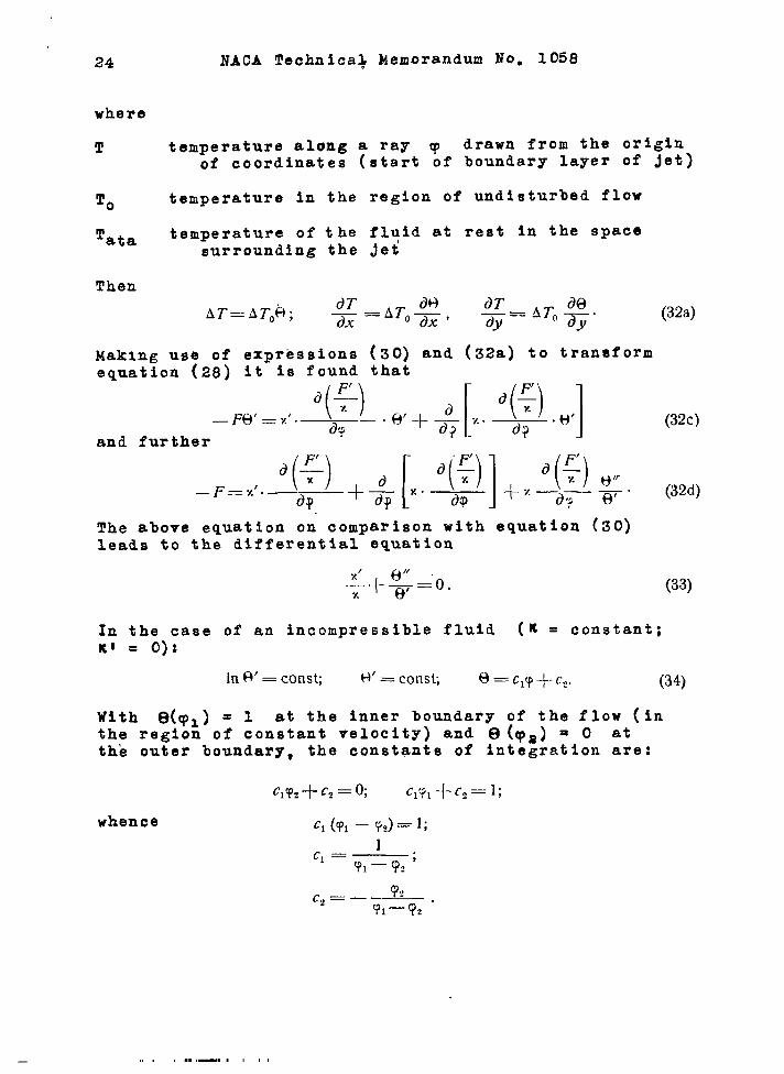
24 NACA Technics+ Memorandum No. 1058

where

T temperature along a ray qJ drawn from the originof coordinates (start of boundary layer of jet)

To temperature in the region of undisturbed flow

‘ata temperature of the fluid at rest in the spacesurrounding the jet

Then

AT=ATo~l;dT

z=ATo~, ~=ATo$. (32a)

Y

Making use of expressions (30) and (32a) to transformequation (28) it is found that

—~~’=.’. ‘\:L.e.l_+[x. ‘{f).”] (32c)

and further

The above equation on comparison with equation (30)leads to the differential equation

;+g=’o..-— (33)

In the case of an incompressible fluid (K = constant;K~ = 0):

ln~’=const; t-i’=consfi e=cly+-c,, (34)

With E3(qa) = 1 at the inner boundary of the flow (inthe region of constant velocity) and O(qa) = O atthe outer boundary, the constants of integration are:

c1y2+c2=o; c~<, +(-,=l;

whence c~(f-j — yJ=l;

c2=— %%-92 “

,, , , .. ,—,, , , , ,

NACA Technical kemorandurn Now 1058 25

Brom this the law of temperature distribution in theb.o.undar,ylayer of a..plan.e-parall.el.flow, of..ap.i,ncom-pressible fluid is found to be:

(35)

!l!heobtained linear law of temperature distributionis satisfactorily confirmed by Rudenls tests (fig. 2,reference 12)*

A certain amount of disagreement with the testsoccurs only at the boundaries where the temperatureprofile departs from a straight line and passes smoothlyover to the boundary values of the temperatures= Thethermal boundary layer is found to be somewhat thickerthan the dynamic boundary layer. This fact is explainedby the following reasoning. The linearity of the temper-ature law is obtained on the assumption of purely turbu-lent heat transfer with the molecular heat conductionneglected- This assumption was based on the analogywitil the dynamic problem where the neglecting of themolecular viscosity lei to a velocity profile which wasexcellently confirmed by tests, A specific character–istic of the veloclty profile was that near the bounda—ries of the layer the velocity gradients and also thefrictional stresses were so small that allowance for theviscosity could have no appreciable effect on the deform- .at ion of the velocity profile. In contrast to this thetemperature field was obtained with large gradients nearthe boundaries. This indicates that the molecular heatconduction at the limits of the dynamic boundary layer isof appreciable magnitude so that the temperature fielddeparts from the straight line law and the thermal bound–ary layer will be thicke’r than the dynamic. Subsequentlyit is attempted to perfect the temperature distributionlaw in the free jet by taking the molecular heat conduc-tion into account. For the computation, however, of thedensity and velocity fields in the boundary layer of afree jet such refinement of the temperature law is notaustified since the accuracy of the density field willnot thereby be appreci:.hl.y increased while+the mathemat-ical labor will be coilz.:~.er~’.ly completed.

OU the basis Of the foregoing it was preferredto investigate the laws of flow in a compressible fluidwithout allowance for the effect of the molecular heat

26 NACA Technical l!iemorandum-No- ,1058

conduction and to restrict the problem to the solution “’~of the previous differential equation: ,.. .,

K’ @n’—-i--= oK“ ~1

whence

f in (K 6!) = constant

and

K 61 = Cl (36b)

The further .solutiop of:equation (36b) is predicatedupon a relation I?etween ,the density and temperaturefunctions. With this in mirid Clapeyronls equation isused$ ,- :

P1

= ~.~ P T-

(“(“36c)

P. =.g:f?o To-J

which in the case of a free Jet with constant pressurealong and at right angles to the flow (P = P. = constant)leads to inverse proportionality between the absolutetemperature and the densities:

P T“. Tata + ATo ,-. = — = .————-Po T ‘ata + ‘T

whence

P ‘ata + ‘ToK=--= -————-.—.Po , Tata+9 ATo -

(36d)

(36e)

Nondimensional parameters. characterizing the degree ofheating (or cooling) of the jet are introduced:

NACA Technical hemoranclum No. 1058 27

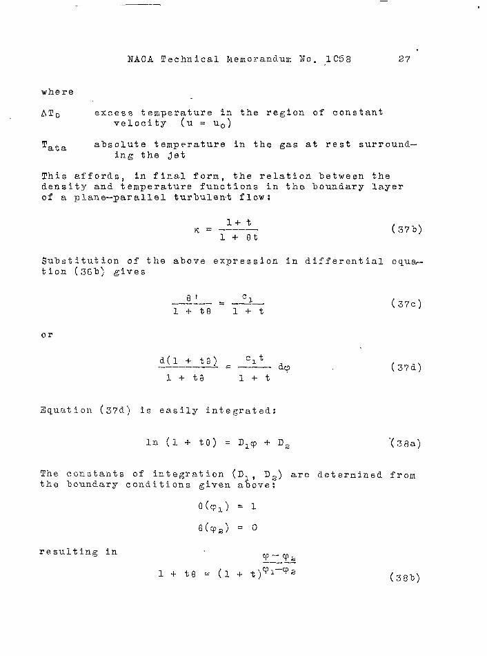
where

ATo excess temperature in the region of constantvelocity (u = uo)

‘ata absolute temperature in the gas at rest surround-ing the jet

This affords, in final form, the relation between thedensity and temperature functions in the boundary layerof a plane-parallel turbulent flaw:

l+tK = -–––––

l+flt(3’7b)

Substitution of the above expression in differential equa-tion (36%) gives

fjl c1———-— = -———l+te l+t

or

d(l + to) c~t——..— —— = ———— dpl+ta l+t

(37C)

(37d)

Equation (37d) is easily integrated:

in (1 + te) = Dlcp + Da ‘(38a)

The coristai~ts of integration (Dl, Da) are determined fromthe boundary conditions given above:

O(qlj = 1

f3(q2) = o

resulting inY–’va——___

l-1-te = (1 + t)vl–% (38b)

—— —. .——.—- .- .——_.

28 N.ACA Technical Memorandum No- 1058

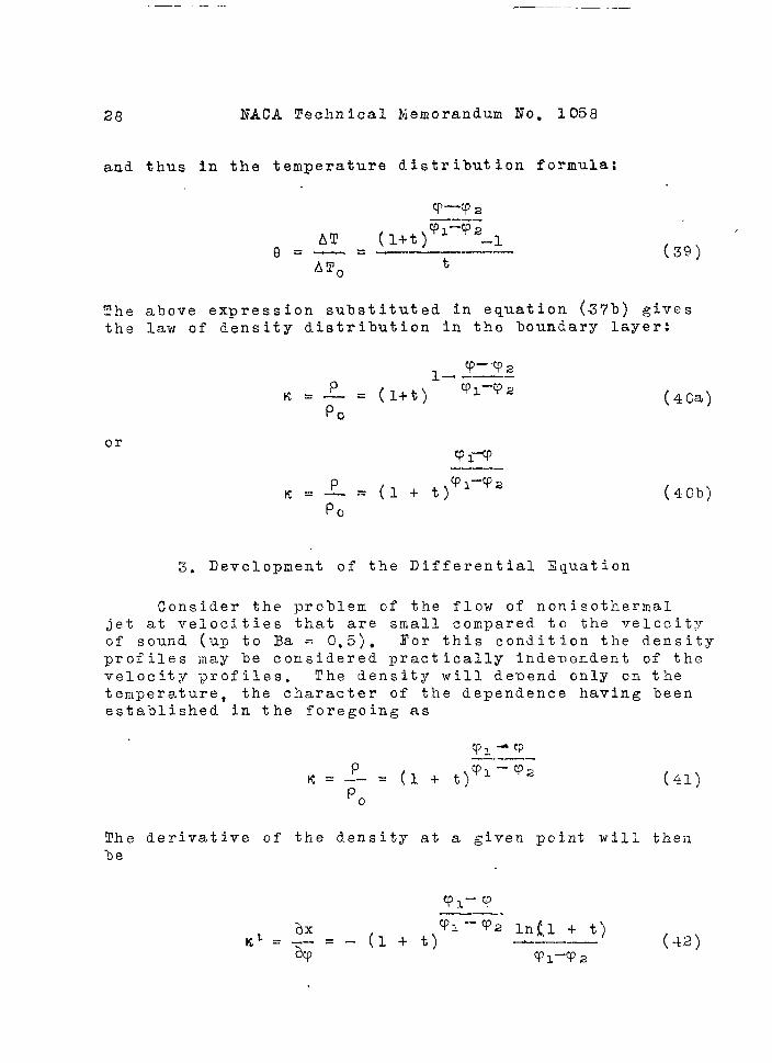
and thus in the temperature distribution formula:

T—v 2—— ___

AT(J. — = {l+t$”-%-— ——— —-—

ATO t(39)

The above expression substituted in equation (37b) givesthe law of density distribution in the boundary layer:

T–”V2. .——p

K (l+t)l Vi–v 2=—= (4ca)Po

or

KP=— = (1 + t)q’-v’

Po(40b)

3. Development of the Differential Equation

Consider the -problem of the flow of nonisothermaljet at velocities that are small compared to the velocityof sound (up to Ba = 0,5), Yor this condition the densityprofiles may be considered practically independent of thevelocity ‘profiles. The density will demend only on thetemperature, the character of the dependence having beenestablished in the foregoing as

??l-V————P

K.=–-= (~ + @l-T2 (41)P.

The derivative of the density at a given point will theilbe

91–V— —.

@=~x= V1 ‘V2 ln[l + t’)

-& - (1 + t) —---—V1-+P2

(42)

..>


!Che ratio of the derivative. ox the density .to. the -value“--. -of the latter will be constant for a given value of the

,jet-temperature..

.,.

K’ - ln(l’+ f) ‘-”-- = . ——--—K. (43)

91 -v-z” - “

Returning ‘to the’ general “diffe~ential equation (20) ofthe boundary layer in a compressible’ gas stream: .

its special form fw? a nonisothermal jet of moderatevelocities is obtainsd as:

ylll=_~_ ln(l+t) ~n

91-92

(44)

(45)

After introduction of a special notation for the parameterwhich depends only on the temperature of the stre,am:

~ = In(l+ t)———.— —— (46a)91 – V’2

The differential equation will then have the following forw

The alove equation is a common linear differential equationof the third drder whose general integral is of the form

,-where

c C2,1s C3 constants of integration

(46c)

k kz, “k~1s roots of the characteristic equation

. —

...- —---- .————. —

30 NACA T,echni.cal Memorandum No, 1058

k~+ak2+l=o (46d)

which in this instance reduces to the equation by Cardan,As is usual for jet boundary layers equation (46c) hasfive boundary conditions.

1. At the inner boundary of the layer where cp = ml

(a)

(b)

(c)

The gradient of the momentum is equal tozero;

~~=o – that is, T“(ql) = o ‘ %)ap

The momentum is equal to the momentum ofthe undisturbed flow:

Pu .= Pouo- that is, Yl(cpl) = 1 (462)

The transverse component of the velocityvanishes:

povo = o – that is, ~(ql) = V1 (463)

2. On the outer boundary of the layer where q = qz

(d) The velocity gradient is equal to zero:

(46 ~)

(e) The velocity is equal to zero:

Pu=o – that is, Fl(qa) = o (465)

The five conditions (461_5} are used to ascertain the threeconstants of integration Cl, 02, C3 and the values of the

—--—. -—-,,.,,,,,.,,,,.. , , , ,,, , ,,,,,, ,,,,,,,1, , ,, , mI . , , , ,.,,,,,.. --. —., —,-,...,,,.- ——..-,., , , ,,... ,

— — _——1~

—

NACA Technical Mernorandurn No, 1058 31

nondimensional coordinatf?s of the-outer and Inner limits

of ‘he ~-oundary layer 91 and Va. ho each value-of thecompressibility parameter S there corresponds certainvalues of the constants of integration and the nondimen-sional coordinates.

4* Integration of the Differential Equation of

the Nonisothermal Jet

According to the foregoing the boundary layer of thenonisothermal jet is characterized by the differentialequation .

.

~fll+ s~ll+)jl= () (47)

the integral of which is.

F= Clekl~ + caek~~ + G3ek3q (48)

The values of kl, ka, k~ entering this integral are theroots of the characteristic equation

k3 + Skg+ 1 = O (49a)

By means of the substitution

–sk = I-—

3(49b)

the given cubic equation is reduced to the Cardan solution:

X3 + 3PX + 2q = o (49C)

in which

P=-S2

q =s’+~ ‘“’ (49d)

The roots of this equation are determined by the Cardanformula:

-.—.. ., . ,,-

32 NACA Technical

xl = u + v, X,2 =“WIU +

the terms u amd v being

r—.—_.—..———-—-—-—U=3 - q -;+ .J?&-+.P 3;

Memorandum No, 1058

W2V3 X.3 “=-’’W2U+ Wlv ‘.-7

‘given

v=

lly ‘., ,4

#

.——-— —--- —-———-

The coefficients ‘WL an’d Wa aTe th’e conjugate irnagina.rycube roots of unity:

J.—

_~’+i 3-’ ““ ““i J 3’W1 = 2

--— ; Wz=-— — i———2 2 2

f,,’

In the present case:._. -—— ———-. _—— —.-.--. —. —_————— .

]1.—.-.——-——-——-——

3u.-

J’s’ + q + [s3”+ g’ - s’

2)

L -: .

\

(49f)

(50a)/-—- —————. ———-_—___ ——.____ —_—___—

,{ ———————_——

IL; q- /’~~+:]2-s’v=3.-. s3+—

w L JSince u and v are real numbers, Xl is the real root ofthe Cardan equation (49c) and X2 and x3 are the con,ju:;ateimasinary roots. Correspondingly kl is the real root ofthe characteristic equation (49a) and ka and k“ the con–ju~ate imaginary roots.

Setting:

\ inte~i”a,l{48) is transformed into

= Cle%~ -i-Cze (a~+~zi)v + C3e(az–@Zi)VI’(cc) (50C)

As is known a pair of conjugate imaginary solutions of alinee.r differential equation of the third order defines apair of real solutions expressed in terms of trigonometricfunctions:

—. —

. .

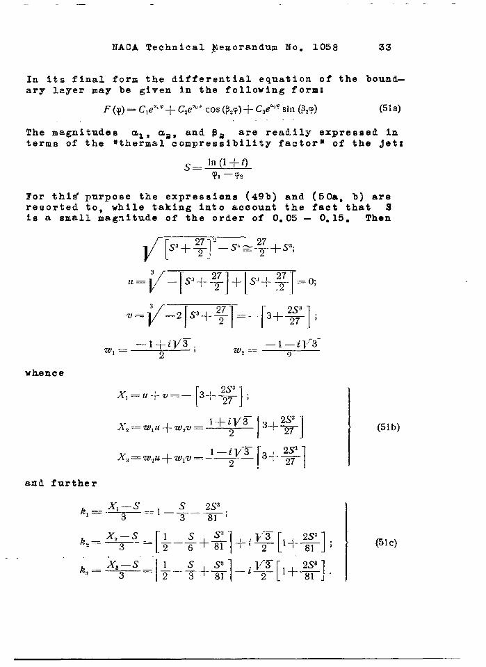
NACA Technical ~,emorandum No. 1058 33

In its final form the differential equation of the bound-ary lzyer may be given in the following form:

F(y)= C,e2’f+- C,e”’cos(p,q)+ C3e*’7sin (&) (51a)

The magnitudes % a a=, and pa are readily expressed interms of the flthermal compressibility factorn of the jet:

For this! purpose the expressions (49b) and (50a, b) areresorted to, while taking Into account the fact that Sis a small magnitude of the order of 0s05 - 0.150 Then

.=~pp+gj-=--p+%] ;

whence

[ ~1’Xl=u+’v=— 3J-

)

I

Lyz-=Wlu+W2V=“’+iv3- [3+%1

(51b)

X:,=W2U+W,V= l-% ls~”%q

and further

~_-x,—s==l s 2s’l— 3

—.

~=x,—s—. =!? 3 [ I3sl~_,iq[l,~];(51,):—~+ 81

IF--$%l-’%z[l+%

; = x,-s-=- 1:{ 3 u

—

34 l’lACATechnical Memorandum Noc 1’058

A com~arlaon of equations (51a) and (51-U) yields theformulas for computing al, Ua, and Pa from equation(50c) for given values of the compressibility factor:

In the particular case of an incompressible fluid,s-o , it is

v%al=—], %=;, ($=--?

which is in complete agreement with the correspondingTollmien solution:

(51e)

Estimating the order of magnitude of the individual termsIn equation (51d) It Is readily apparent that the termscontaining (Ss) can be neglected since S is usuallyconsiderably less than unity. Thus , for example, If thetemperature of the Jet is 100°C higher than the s~rroundingtemperature, S will have the value 0.1 and Ss = O.OO1OThus without appreciable Impairment of the accuracy

s 1s l::a.=—- —, ;j2=——U,=—l--–—, - ~

3 3 2 (52a)

The basic function of the boundary layer then assumes “the following form:

The expression in braces corresponds exactly to the Tollmiensolution for an incompressible fluid:

The first derivative .of F(cp), equal to the nondimensionalmomentum, ia given by


The second derivative of F(q), which is the nondimensionalvelocity gradient, is

For these considerations the factor $a/~ in the fore-going equation are neglected.

There remains, on the basis of the five boundaryconditions (46 ~-~), the determination of the constants

of integration Cl, Ca, C~ and the values of the non-dimensional coordinates of the outer and inner limits(VI) and (cfa) of the boundary laYer:

~(?l)=%, F’(+I)= 1, F“(~l)=o,

F’ (+)= o, f=’’(~,)==o

The problem of predicting the basic function F(cp) iSthen solved,

!Che five boundary conditions lead to five transcen-dental equations with five unknowns (Cl, Ca, C3, qi, andqa) solvable for any particular value of the compressi-bility factor. By applying the transformation of variablesproposed by Tollmien

(53a)

these equations can be considerably simplified. The sub-stitution is made so that

36 l!ACA Technical Memorandum Ho. 1058

F (~)= F(Y), F’ (~ = F’ (~), F“ (+)= F“ (?)! (53b)

Then .

and

—

s

[ II.—-

F(j)= e–Tf D,e–~‘+D,e-ices .~? +D.1e;5jn[~?l]$ (53C)

hence, while bearing .In mind that, —

five equations with five unknowns:

F,,, = Yl; s‘@’’—3F~1 = 1; FO1’’–$F’ ==0; 101

I

1

(54a)

&’_-$ j-F —().0]— ! F,,z’f–~F’ =002 9

which are simplified to

With the first three equations of the above system thecoefficients DX, Da, and Da of equation (53c) can beexpressed in terms of ql:

—D,++(D,+D3V%)=1+;; (54C)

Q++,17=D)=$. (54d)

fr?OEIwhich

Dl= %-13 +;; D,=?1+0,5 S——. .

1,5 9’D3=~_+&.

~3(54e)

With equations (54c) the five equations of (54b) (withaccount taken of equations (52) and (52e)) can be reducedto a system of two equations with two unknowns:

—Die–(y’-v’)[ 1+~(D2+D, V@ey’~v’cos ~(q, –vl) –

(Q,‘Q,)‘}[DzV~—DJe 2 sin

[

V-3—-97(?2 -%) 1=–0,13s; (54f}

——

J!IACATechnical Memorandum No. 1058 37

where DX, D~, .and-D~ are taken, from equations (54c). .’Addition and subfraction of equations (54f) and (54g)give two Eew equations of a somewhat simpler form:

,., an[

)?1- v,——-

D:,~e 21

3-(?2—%) —

[

‘ —,in ~3-% — v,—D,~r3e 2 ~($2-–%)

1=—0,13s;

!1 (55)

Rext it is attempted to determine the functional relationbetween the constants Dl, Da, Da, ql, and q= and thecompressibility factor S making use of the fact, eswill be shown later, that the compressibility of th”e airis of only slight effect on the free Jetc Putting

D,= % + AD1; D,=D2~+AD,; D,=D30+AD~\

% = %0+ %’1; ?2= f?zo+ A?2) J(56a)

where Dlo, Dao, Dso, Wos and q are known value~ao

of the constants for the incompressible Jet:

~io — 1DIO= ~ =—0,0062,

D,O ===—;T = 0,578,

. - P.-?.-4. -’=--- -=.+. ~ . * - .,. . . . .

D20=?10+0’5=~9871,5 ‘ ‘

1 (56b)

%0= 0,981;Y,O= — 2,04,I

. ..

and the smail.incr-emeats (compare equations (86a) and ‘‘86c) with (84b)):

38 NACA Technical Memorandum N.n, 1058

Reverting to equations (55) expanding into series whileneglecting all terms of higher degree than the second andthe products of the small increments and using the values

1951= 4.51

3.02e e = 20,4

sin(-2062) = – 0.5, COS(-T2.62)= – 0.865

results in

0.082S.= 0.380 Aq2 v 0,255Avl

4,634S = 0,130A(p2 - 13.60Ay1

The solution of these equations leads to a functionalrelation between the deformation of the boundary layerand the compressibility factor:

Aql ~ - 0.34S; m 2 =0 (5’7a)

which yield the corrections for the integration constants:

s $ADI : O; AD2 = -; AD3 = —

9 1,7(5’7b)

The constants of the auxiliary function 3?(;) are thenequal to

Dl = - 0,0062, Da = 0.987+ 0.11S; D3 = 0.587+ 0.59S (57c)

and the ordinates of the outer and inner limits of theboundary layer

V1 = 0.98 - 0.34S, ~z = – 2.04 (58)

—

,,

I?ACA Technical Memorandum’ No. 1058 . 39

..-. -Equations (5’7e) and (58) give the integration constantsof the fundamental function F(q). The first threeboundary conditions of the given problem are used:

After substitution of the. values’- T, l?~ and F II fromequations (52b), (52d), and (52~) the first boundarycondition gives

,,

The constants of the compressible gas are again expressedin the form

cl= Clo + ~cl, C2=C20 + AC2, C3 = C30 + AC3 (59c)

where

.

c 10 = – O“.0176, Cao” = 0-1337, C30 = 0-6876 (59d)

are the corresponding values of ‘the constants obtainedby Tollmien for the particular case of an incompressibleflow* In the same manner, according to (58) the coordinateof the inner boundary of the layer may be written:

VI = Vlo,- o~34s’ (59e)

where cplo = 0.981 is the coordinate of the inner boundary

for the incompressible fluid. ~tibstitu-tion of (59c) and “(59e) in (59b) and use of the series up to. the second powerterm (due to the smallness of, S) of the exponential andtrigonometric expressions gives

:,

40 NACA Technical Memorandum Noa 1058 ~

‘in[=,l= sin[-~’lol- ”*3’’o’[-~lol.

~ (59f)

The products and squares of small terms are disregardedand the following relation is taken from the boundaryconditions for the incompressible gas:

wheilce the equation connecting the increase in the con-stants due to the compressibility with the compressibilityfactor S:

0-375 ACl+ 1.09ACZ+ 1.225 AC3 = 0.340S (60)

The second boundary condition Fl((pl) = .1 in combinationwith equations (52d) and (593) gives

(61).,

Substitution of expressions (59c), (59e), and (59) inequation (61a), while neglecting products of smallquantities, and making use of the particular form ofthis

——, ,,..,,

equation obtained for incompressible gas yields:

,.,..,,,,.,- ,,, ,,1,,,11111 11111111111111I■ llllmllmlmm¤mfi~-m~ ■ lmlmlnIIlllllnIm Ill

.

NAGA Technical Memorandum No. “1058 4-1

a second equation for the relation between the incrementsin the constants o’f‘the function” F(q) and the compress-ibility factor: . .

-0.375ACl – 0a52AC2 + 1,55AC3 =’0.654 S (62)

The third boundary condition F1r(ql) = O, together withequations (52e) and (61), gives

BY substitution of expressions (59c), (59e), and (59f)in equation (63), while neglecting the products andsquares of small terms and taking account of the factthat in the case of incompressible gas equation (63)assumes the form:

. .. ,.

the third relation between theof the function F(q). and the

increments of ‘the constantscompressibility factor is:

,’‘,.!.

0.375 AC1 - 1-6 ACa + ().32 AC3= ().332s (64)

42 NACA. Technical hernoranduni No.’ 1058

The solution of the system of three simultaneous equa-tions:

0.375 AC I - 1.60 ACa + 0.32 AC3 = 0.372 S,)

-O-375 AC= - 0.52 AC2 + 1.,55 AC3 = .0.654 S)

(65)

0.375 ACl + 1.08 ACZ + 1.225 AC3 = 0.340 SJ.,

gives the laws of variation of the can.staits of integrationof equation (523) und’er the effect of compressibility:

ACI = O, ACZ=-0,14 S, AC-3 = 0.385 S (65a)

hence the integration constants:

cl=- 0-0176; C2 = 0-1337 - 0.140 S; - .

C3 = 0.6776 +Oa385 S (66)

Substitution of expressions (52b) and (52e) in (66) whileneglecting the products of small quantities, the function1? and its derivatives are obtained in the final form

.’

F= FO+AF; I’~=Flo+AF!; y !1= yllo + AFn (67)

. .where Fo, Foi, and Foil ‘are the -values of the functionsand its derivatives for incompressible gas’ (Tollmienlssolution):

g-.

[

4’v—

Fe(q) =– J0e0176e-V+ 0.1377e2 cos $&&p + 0m68?6eZsin ->q

1

1y

J

-

[

yFor(q)= 0e0176e–V+0. 6623e2cos f-~cp + 0.228 ez sin –2ZT

1(67

2v

[

J?w

rol~(q)= -Oe01’76e-q+be528eacosz

-2-W –“ 0.930e sin ~~2’,

and A.F,.~$’1, and AYn are the increments of the functionJand i%s derivatives under the influence of compressibilityThe increment of the function is

.... ,,

NACA Technical Memorandum Noc ..1058 43

... ,>. .,.~ .,. .

AF=–;[

; J

[1qFo+ 0.q2e cos & -1.16 e;cosr~q’ ‘(6’7b)

[ 1]J

that of the first derivative ‘

and that of the second derivative

., ,. v v,

[

AI’n.- : ~~o tl+2j70 1

[1

45 “3– 1.2eZcos –2–cp

@

[ 11+ Oe22e sin -—Zv (67d)

3

In conclusion it should be note? that the authorlscarefully conducted numerical “s.ol~tjc,n,based di:ectlyon equations (55), showed c{)),:m~e~~~:yeement” wiih thefunctional results, (F7a) aI.d”(67m\, e,pproxirnately obtained,notwithstanding the fact that for the numerical solutiona vcr’y large value vas chosen for the compressi-ojlit.yfactor (s= 0.135) corresponding to the case whsre thejet has a temperature 150°C above the surroundirig temper–atureo

It will be recalled that the first derivative of thefunction F is the momentum of the flow in the directioilof the X—axis;

.

(68a)

TO obtain the velocity u/u. it is necessary to apply tothe law of density distribution in the boundary layer:

,. .,Vi—v————

\,- ... ...-.!, ,.- ,.,

W =“;p~”=.~l+t)wvz

o(68b)

then “ ‘..

u Ft—=—‘u0 K’ (68C)

. .

44 NACA Technical .Niem.crandurnNo. 1058

The momentum velocity ratios in the direction of they-axis are

To facilitate the computation of the components ofthe velocity and other characteristic magnitudes of thenonisothermal layer, table I is appended with the computedvalues :

The tables 2, 3, and 4 contain the values:

F1 ~F~-FF, Fl, FII, K, —; –——;

% K~~t - ~ ;!, e

from which the velocity profiles, velocity heads, den-sities, and temperatures may be computed for the follow-in~ values of the cop.pressibility factor:

s =— 0.074; s = 0.0605; s = 0.1115;

the given values of S corresponding to the jet temper–atures of —60°, 60°, and 120° C, respectively, abovethe surrounding temperature,

5, Fundamental Properties of ~oundary Layer

of Nonisothermal Je’

(a) Geometry of the Je&

The nonisother~al jet, that is, having a temperatureother than the surrounding space has, as explained in theforegoing, the interesting property that. its outer bound–ary (u = O) remains constant for variation within verywide limits of the temperature increrlent (At = * 150° c):

CD2= constant = — 2.04 (69)

. ..,.

NACA Technical hernorandum No. 1058 ~ “ ’45:., .,.,’

The -inner. boundary, (u.!=}Uo) expand”s somewhat when thejet is cooled and compresses when heated:

91 =’ 0.981 - Oe34S (70). .,

where

ln(l+- t)s = -———. compressibility factor of the jet

V1 -V2

‘,t = Ato/Tata - ratio of the temperature increment (At in ‘c)

to absolute temperature (Tata = 27’3 i-t~tao C) of the surrounding fluid.

Accoi-ding to formula (70) tlie following results areobtained: At = –60°; cpl = 1.005; At = + 60°; cpl = 0.960;At = + 120°; cpl = 0-942; At = 0° —VI = 0.9816

The nondimensional width of the jet boundary layerdepends on the temperatw.re difference above the surround-ing ter,perature in kne following manner:

<=~=3.02- 0.34 sax

(71)

The boundary that se-parates the initial mass of thejet from the entrai~ed mass is deter~,inecl, as is known,from the conclitioil that at the partition surface (Cp3)the stream function ~3 = O, or, what amount”s to the samething, I?(Q ) = 0. The relationship between the boundaryof the core30f constant rna.ssflow of the jet and the com-pressibility factor was obtaineii as follovs:

In the case of incompressible fluid it is’

ro(qY30) = o

For a compressible fluid

1’= F. + AF, 93 = T30 + AT3 ‘-

then

F(q3) = Fo(q=)+ AY(y@ = Fo(q)o+A@+ AF(V30+ Aq3) ~Fo(q),)

+ Ac@ot(cpo )+ AF(V30) +ACP3AF’(V30) = O


Omission of the small magnitudes of the second order(Aq, AFT) while -bearing in mind that

Fo(cpo) = o

gives

AF(CPo) +AcP#o’(cPo) = O

hence

~ 0.52AF(v=G)_ ~ 3 “__ g 0.29 S

Aq =--–3 ~o%o) 0.59

The result is the formula for the boundary of the constant

mass flow core:

v= - 0.185 + 0.22S (72)3

The same result is obtained by direct interpolation fromtables 2, 3, and 4*

(b) Velocity, Temperature, and Density Profiles

In the representation of the velocity profiles themagnitude

q—cr~

v= —-———---Y1 - V2

serves as ordinate, the effects of heating and cooling “of the jet can be compared from the plotted velocitydistribution curves. The curves shOWn in figure 3 arefor At = + 60° C, -60° C, and + 120° Cc

On figures 4 and 5 are shown the density and temper-ature fields in the jet boundary layer for At = - 60°and + 60° Cc

NACA Technical Memorandum Xo. 1 058 47

66

gi00

ves the field ?fc:

velocity h..ead sfor

pu2---—POU02

Jjl,2-— (K

Figure 7 finallyfields for At =

giv-6

es0°

thec:

fields of transv erse velocity

v——

V. = (;)

!Cheiccto

respondingressible fluor com.paricc

fiel~s obtained by T(>llmi’:.lfor the!& (c,,,;= O) are shofi’~1in “ig~~es 3lL* (p~e tables 11, III, :Li’.d IV.)

(

?he quantityco]ll~>re~siblejet <Lof the strea,m functhe density. The

—.—ml ‘j-p udy = j’

But the stream fun

c) Rate of kass Flow

‘j.sch:,~ged p~rL.. second in the turbulent.>s not e;.~lrely correspond to the valuestj on on accl>dnt of the fluctuations inillas~flow per second is

——__ -——_fJudyi-j plllrdy =~~ Jpluldy: (73)

ction is cletermined by the expression

w axpou.oF

while

(FI

a )T!—,)—.-

?Xp,..au

-&up OUo

so that the r,ass flow per sec ond is

“)–d

[

F+a 1 constant1

(’74)m ax pOuo +

I

.!, , . . ..—— --—- ‘1

48 NACA Technical memorandum Nom 1058

or in nondimensional form:

In particular the nondimensional value of the entrainedmass of fluid sucked into the free jet from the surround-ing space is*

aFI

2

ij

()‘K-/ 1E2=— F2 + a n ~! –—–-dcp

@ J.3

The nondimensional magnitude of the retarded mass offluicl in the initial jet core is

(76)

(77)

The values of F2 and I!’lmay be obtained from tables ofintegrals and %y approximate integration (for example, bYSirnpsonis method) the values of the integrals:

(79)

for various values of the temperature of the flow. Further–more, assuming a few values of tile turbulence factor a,for example, taking a = 0.0845, according to the tests ofTollmien, it is not difficult to determine the values ofthe mass of the initial jet and of the entrained mass forvarious values of the temperature.——.———__ _——-———————————.————__——-————-——__.-_———__*The subscript 1 hereinafter refers to the boundary ofthe region of co~stant velocities; subscript 2 to theregion of fluid at rest; subscript s to the core ofconstant mass flowe

—.. ——-


The integral in expressions (76) and (77) may beintegrated by parts:

From the boundary conditions it is known that

~~oreover, according to equations (41) and (46a):

Vi-v

K = (l+t)q’-qa; ~ = ln(l+t)Cpl–Vz

hence

Omission, as in all parentheses of the preceding section,of khe terms with factor S2 leaves

whence the expression for the entrained mass:

(81)

A glance at tables II, III, afid IV correspondin~ toparticular cases of the nonisothermal jet:,,

s =- 0.074 (At. = - 60° C)

S = 0-0605 (At. = + 60° C)

s = 0.1115 (At. = + 120° C)

50 MACA Technical ljemorandum No. 105.8

shows the values of Fl(q# corresponding to the

particular values of the compressibility factor Son the assumption of a = 0.0845 for the coefficientof jet structure (turbulence) - according to the dataof Totlmien and CAHI Therefore .

., -. .

a S FI(q3) : 0.05 S (82).,-

The values of ~(va) for 92 = --.2.04 is computedaccording to formulas (67) and (67b):

~(q2) = - (0.388 - 0.27 S) (83)

Lastly equation; (82.) and (83) added together give thefinal expression “for thenondimensional value of theentrained mass of the jet:

5i2 = 0.388 + 0.22 S

The initial mass of the jet is3

~ ~J

l?li ‘J(x

=Z1=F1+(Z x’. ) .d~=axp#,, d?1

(84)

(85)

Ac-cordfng to (79)1

x “—=s’20; +==—s,

v.

hance

fil=F1+mSIF’l —F’.J,-FI- 0,034S. (86a)

~urther, equations (67) and (67c) give

F,= 0,981~ A~(Yl)~ 0,98+ 0,02S. (86b)

Substitution of (86tI) In (868) yields the final expressionfor the nondimensional mass of the initial part of the jet:

fil=Oj981-0,01.4S. , (87),,. . . .


The total (nondimensional) mass flow in the boundary layeris eaual to

The smallness of the value of S indicates that themass flow per second for the nonisothermal boundarylayer differs very little from that for the incom-pressible jet.

(d) Frictional Stress

In section I an expression was derived for thefriction~.1 stresses in the turbulent boundary layer ofa compressible gas, which according to equation (128)can be written

[au d

=2c~x~ ——OIL

7XY ()— G!y+collst,

,,dy dy ‘dy,(89)

But

The nondimensiotial value or tne frictional stress is

.= fi=,~!.g)..+[x!(:-)ld?.,corlst (,(j)

2 *.

After corresponding transformations Dartlal integrationyields

,=..~~j’+(i.[d(;)j:,+c.nst. (91)e.

~Jhe values of ~ of greatest interest &s t~at at theboundary of the core of constant flow ? = 73 since Itdetermined the energy Loss due to suction of the entrainedmass. This value of 7 Is evidently given by

, .—.,. .— . ..! ,, . . .!.--.— . . . . —....———— .


At the inner limit of the boundary layer

~ F’

(-) 7.

d+ ‘0’hence

,,=_X,[d(-$)]+JX+H].,,.d

In addition

. —— ,.’? X2

where according to (79)

~=es($l– u). s(y,-.4’=-~.e %)#

whence

Since the values of S are small

es(cl— f)—l+s(y,—~).—

it results in

~ (q)

d? =F+S(q--ql)F’’+S,’,

[( 1)=’‘)2

d—x)

d? = F’”+ 2S(Y— ~J F’” +2 SF’F”,

[ -)J‘,F -,

( xx —— =p+s(9-y,) P~+2sF’F”;

d?

HACA Technical Memorandum Ho. 1058 53

With the aid of the approximate Integration-method andtable X the integral becomes

.-. -, .(“Fo!12dq=”(j,4“

3

within the limits q) = -’ o.i85 to VI. = .0.981 (tnegiwem Taluaa of Va and VI correspond to the incom-pressible jet). 140reo~er,at the point 93 (for ~ariousvalueB. of s): .“

oF“az.O,52, ‘ f=/:,~o,6.

wheace , ...T3= 0,27— ;0,32+0,62 S+0,4.S.

The final expression for the nondimensional value of thefrictional stress at the boundary between the Initial andentrained masaes of the jet

t,7:1 = — _ :.y

U. = 0,27+ 0,7S,/.zpo——

2

(94)

(e) Hea* Transfer

In section VI fpar. 1) the differential equationwas obtained for the trans~erse heat transfer due to theturbulent fluctuations in the free jet of the compressiblegas:

1 d WT

[

dp du dT d

(

dll dT—— .—Cp.g ay ‘2C’”X’ .7j-”~”7# dy fnj- dy

-—-)1

(95)

~he heat transfer from the’ initialmass to the entrainedmaem acrose 1 ma of partitibn surface T9 Is studiednext:

From previous results

)

s.e(?–Q,)s;

Y=ax~; 2c’=u~; p=p.e(~l–v)s.ap aT *T l+t

———po. f?(y’-~)s;, ~= —“d? — “t

au—.d?

/zOO~(?–%)s lF~/+sF,],


wilence

Use is also made of the known relation

ek-92)5l+t 1—————-- -..-—---—

‘— = ;b-%)s-l = (qyw, )s

+1

t

After certain ,simplifications, while neglecting verysmall terr,s, equation (96) assumes the form:

wry s-fPl

I3

-= _--.-———— -————- -

Cp g p. U. AToa 91 -92 ~

[

1 1 .3

+ –-—–- + sJ

‘ ~tl + ~11 (o_qJs+sFt

V1 -V21

Yurther transformations give

~?T

‘[–––1––-+ s v~ -Tz-——————————-—— a- —————— 1F“(cp3)acp ~ PO ‘oATo 91 –Y2 V1 -V’2

But*

G FoU(q30)+AV3FIJ(@ I?l” (q30)= Foll(@+AFt’(q3)

-I-AF” ((030) = Fo” (m )’30

and , further,

Cpl = q?~o — 0034s

v=– 0.185 + 0.2°S3

(96)

(96b)

(97)

-——————— ———————————.—————._—————————————_——_ -_-———————*In region q the magnitudes -Jl,lland AF t1! as sumevalues of the30rder of zero.

NACA Technical, memorandum No. -,.,

,. ,. .’ --’.,-

The foregoing relations yield.-. . -—

.’. , WT”.—..-—--agcppouodqo,, . .

.’

where ‘>

,, “.

= 0.”52,ti&ip30) . , ,

,.

55

F011(v30 ) + o-34S= -——

●

+’i~’- Tio . .. . ,,

.

91 0 = 0.981,V Tao = -2.040.

Thus ,the nondimen”s~onal magnitude characterizing theheat transfer t“hrou’ghthe ~oundary of’the intial massof the noniso’thermal jet is equal to ‘ >

,,

VT . .,

iiT = -—-——— = 0.172 + 0.34S , (99a)%cpPo o*U A !l?O

The coefficient of> heat transfer from the initial massto the entrained mass equal to the amount of heat trans-ferred per hour through 1 square meter per degree differ-ence in temperature is -

;{ T

aT “~~ = 3600 a g Cp, p. U. ~0.1’72+ 0034S1–-~~A--- (99b)0 m2 hr ‘C

For a turbulence coefficient a = 0.0845 and g = 9.31,it yields

UT = 3000 Cp P’o uofo.172 + 0.34 s) (100a)

For air with a specific heat of the order of.

Cp = 0.24 .

it is

a.Tcal

= 720 PO uo (0.172 + 0.34 S) —--——. (loob)m2’ hr ‘c

The effect of the compressibility on the heat transfer inthe nonisothermal jet is appreciable, For” example, for ,atemperature difference ATO = 60° C (S g 0-07) the heattransfer in the compressible jet differs from that ,of theincompressible fluid by, about 15 percent.

.\


(e) Concluding Remarks on the Nonisothermal Jet ,

As is seen by the previous discussion the effectof the compressibility of the fluid (gas) on the funda-mental properties of the boundary layer of a nonisothermalflow is insignificant. In particular, on lowering thejet temperature 60 0 C below that of the surroundingmedium (this corresponds to an increase in the velocityto Ba = lmO in a jet of high velocities) the angle ofdivergence of the boundary layer increases by 0.7 per-ceilt; the angle of dissolution of the core of constantmass flow increases by 11 percent; the nondimensionalvalue of the entrained mass by 3,7 percent; the massof the initial jet remains practically constant; thefrictional stresses decrease by 16.8 percent; the heatdiffusion is reduced by 15 percent,

The results obtained are evidence of the mainte-nance of the dynamic similarity of the jet for appre-cia-ole changes in its temperature**been shown that if S =

It has furtherln(l + t)/(ql – qa) is taken

as the compressibility factor of the nonisothermal jet, owhere t = Ato/Tata is the ratio of the temperatureincrement of the jet to the absolute temperature ofthe surrounding medium, the change in the fundamentalproperties of the jet with S is linear except for thenondimensional coordinate giving the dissolution of theou”t.erbOUndary of the jet which remains unchanged. Itwill be shown later that the cooling of the jet at smallvelocities has the same effect on its fundamental prop—erties (velocity profile and friction) as an increase iilthe Bairstow number-

IVe BOUNDARY LAY13R OF A PLANE-PARALLEL JET

AT LARGE VELOCITIES

1. General Considerations

!l?heinvestigation so far involved the case of afree turbulent jet having a temperature different from‘that of the surroundings and a velocity small by com—parison with the velocity of sound; that is, the effect--------------------------------------------------*!The similarity of the jet for a wide. variation in theReynolds number was discussed in a previous report (ref–erence 6)0 ‘

NACA Technical hemorandurn No. 1058 57

of con,pressibility arising from the difference in tem-pei-ature alone was studied. The following deals withjets of large velocities (up to the velocity of sound)under the condition that the temperature in the reservoirfrom which the jet escap~s is equal to that of the sur—roundings, or otherwise expressed, the effect of compress-ibility due to high flow velocitia”<”-will be investigated:

‘ 2. Derivation of the Density I?unction

Th? air temperature ahead of the nozzle (in theregion of small velocities) is equal to the temperatureof the surrounding medium. In this case there will beno heat transfer between the jet and the surroundingspace so that the heat content of the air will be uniquelyassociated with the flow velocities (the energies of thepulsating and transverse motions are neglected):

:g (U02 _ U2)CP(T - To) = —- (101)

where

cp specific heat at constant pressure

~heat equivalent of mechanical workA = Z5T

g acceleration of gravity

The relation (101) expressed in nondimensional formgives

(lOla)

The velocity of sound in the region of undisturbed flowreads the value

,—-. —

co = / :2 g R ToJ Cv

(lOlb)


where

Cv specific heat at constant volume

c13/cv = ~ adiabatic coefficient

R gas constant

The Bairstow number in the undisturbed region is

Bao = uo/co and AR = CP- Cv

hence

(102)

The foregoing expression gives the relation between thetez,perature of the flow and the velocity- Particularlyin tile outer boundary of the flow (region of air at rest)where u = O:

At the inner boundary of the boundary layer (undisturbedflow with velocity %):

A thermometer, however, mounted at any stationary pointof the flow will show the same temperature To — thetemperature of the air at rest - since the velocity ofthe flow drops to zero directly at the wall of the ther-mometer. Thus a stationary thermometer in the flow snows—-—-——— ..————-— ——not the actual temperature of tlie Tl=ti-but the temperatureof the retarded air, the stagnation temperature,

The above flow considered from the point of view ofthe stagnation temperature is isothermal as a result ofwhich it was possible to assume that no heat transferexists and to apply the heat equation in form (101)-

NACA Technical I?emorandum -No.’lO58 59

The foregoing problems of free turbulence involveisobars (the pressure gradients are negligible and nottaken into account);.hence the density is inversely pro-portional to the absolute temperature:

o[’-(~;)’l ‘102’)

Po=_T_=l+k–,l Ba 2——

PT0

2

T!lerefore the density function is:

K (q) = -—---- -—-— .—--——.. (102-D)

1+%“; [q, f;jyl

The solution of the above equation for K gives thedensity function in the form

~

.— _———

1+ 1+ ~(k_ 1) Bao ~ (1+ ~;_~B20J’F ,2

K = ( )--——.———__—.— __________________ (103), 2

(

l+k=~ Bao.z2 )

and the ir:troduction of the special function o; theBairstow number:

r[

= 2(k-1) Bao2 1 + ~~-~ Bao21

(103a)

whence the calculation of the derivative of the densityfunction affords

K’ r~?~!l-- =K -—-=====——-——————-G—

J’l+rl?la rl+Jl+r?l’r2J(104)

3= Derivation of the Fundamental Differential Equation

With equation (104) the general differential equation(20) is reduced to the following special form which satisfiesthe problem in question.

60 NA~4 Technical Memorandum No. 1058

?3 ‘p

1r~ 12~11

F!n . . F+.- —-—— ——--—-—1

(105)

J

----— .—--———.av +rFt2, [l +Jl+ rFta]-’ .

whence

and

(105a)

~l~rther transformations yield a differential equationof the form

(106)

In the special case of incompressible flow when r = O(equaticn (106)) reduces, as expected, to the knownTol.lmien equation:

FIll=_F (106a)

Differential equation (106) as well as the Tollmien equa-tion (106a) contains the five boundary conditions (461_5)

which are applied to obtain the three constants of inte—gration and the values of the nondimensional coordinatesof the outer and inner limits cpl and of the boundarylayer. TO each vaiue of the compressibi~?ty parameter (r)there corresponds the values of the integration constantsand nondimensional coordinates.

Since the functional solution of equation (106) isimpossible, it is necessary to apply the method ofnumerical integration to each particular value of theco-repressibility parameter (r) or what amounts to thesame thingl the Ilairstow number {13a). The most suitablemethod for solving” the given equation appears to be theAdams method which gives good agreement for the given case.


4. Numerical Integration of Differential

Equations by the Adams Method

If the values of a function and its derivativesat a certain point are known, the values at a neighbor-ing point (a + .h) can be obtained with the aid of the!laylor series. After the values of the functions andits derivatives at the point (a + h) are determined, thevalues at other neighboring points (a + 2h), and so forth,can then be found, In general’if yk = Y(a + kh) is knowil,then

‘k+l = yk + hY~k +2: h=yftk + ~~ ylllk+ ...

21

Thus , passing successively from point to point, it ispossible to compute a table of values-of the requiredintegral, that is, of the required function Y(x) overthe entire integration range. The smaller the size ofthe interval h the mere accurately are the values ykdetermined although, on account of the large number ofintervals, the accumulation of errors may become con–siderable unless a sufficient number of terms of theTaylor series ‘is employed- The fundamental disadvantageof Lhis method, which wa”s proposed by Euler, is that itis necessary to ccmpute the h“igher derivatives which,for arbitrary form of the function Y may y’ield verycomplicated expressions. In such cases CL considerablyless complicated method is that by Adams in which theincrement in function at a certain interval is expressedby the first differences in the so-called lf.near incre—ments of the function, the second differences, in theneighboring intervals, and so forth. The Adams methoddoes not require the higher derivatives and gives goodaccuracy even for large integration ranges. Particularly,as will be shown later, in solving the differential equa-tion of motion for the compressible gas jet (equation(106)) - the Adams method gives very good agreement..

. . . .The linear increment in a certain interval (a, a+h)

is given by the product,. .

. . .

.. .

..

.. :.,’.-.,: .-. ; .- -

. . .., ‘

62 NACA” Technical Memorandum No.’ 1058. .>

The first difference of .thq linear increments of thefunction in neighboring interva-ls. is given by

... .

The~second difference by

the third difference by

A3qn_3 = A%n_m – A%qn_36

and so forth.

In general if there, is a table of values of therequired function at n+l points it is possible todraw up a table of linear increments at n+l points,first differences at n points, second differences at(n - 1) points, third i$ifferences at (n - 2) points,and so forth. The Adams method makes it possible tocompute the value of the f~n~tion> at the (n + 2)thpoint, the value of the linear increment at the (n+ l)thpoint, the value of the first difference at the ntn point,the value of the second difference at the (n - l)th point,and so forth. By the same method it is possible to proceedto the (n + 3)th point, and so on up to the end of theentire integration range,

The extension of the integration table from oneinterval to the next by the Adams method i.s effected onthe basis of the following considerations:

1. The Taylor series affords the increment in thefunction: ~

ha hs

AYn = Yn+= -Yn= hYln+YY ln+—-Ylrln+c .,6

2. According to the definition of the linearincrements

NACA l?echnical M:em,~randum No. 1058 63

3.valu

Appes o

licqtion of the Taf the derivatives

orth

series results in,e foregoing intervals:the

yll +n

.h=_,-—6

IVYn Yv-y!n - h y 1 Ilnt

n-i+ ‘.**

2hYltnIV 16

+: ha,”yllln_ & h3yn +_ h46 24

Yv– .Y 1n— 2 . .

h2yll!n

IV.i13Yn + h4 Yv– .yl

n3h y II

.n + . .

.

ous values”ts gives

ion ‘of thlinear i

epncr

reviemen

in the ex—Substits for t

UtheP

?on

h=.-2 Y

h?

-E-YIVn

hsZZ

*V

n=h yin_ Illn + .**n—l

Iv v.$ h3y:ll - : h4Yn + = h5Yn. 24 —...

5. definition of the first and hi gher differences

nn – 1

An- nn- 211n + mn— 22 n- 2

A3q L’Aln_2 Az~n_3

,’

11n– + 3nn_-3 21

60 Substitution of. the expressions obtainedthe linear increments in the differences yields

for

64 NACA Technical hemoranduin No. 1058

7. Next it is shown that the true increment in thefunction may be expressed i% )erms of its linear incrementsand differences:

.

For this purpose the coefficients a, ~, and Y are com-puted by comparison of the Adams series (107’) with theTaylor series:

>.-

1- 3 4 IV 5

AYn= qn + a ~h2 Y!In-> 1Ytlln++y ~_;zyv .+nJ

r+$

1

hs~f Iln’41V

-h Y &:h5 Yvn1

’41V 5V1+y~h.Y n-~hYA L n]

This may be done by equating the coefficients in the twoseries of terms of the same degree in h, which thenyields the following system of equations:

To defermine the coeffac~e.n.ts-.,the--firsthreeee quationsns!..%..“./dm.+-.4...,..--&-are er,ployed; then

..) .,

2 12 8

From the fourth equation the order of the computationerror may be ascertained. In the given case the errorwill be of the order

●

BY taking, in order to increase the integration accuracy,a term with fourth order difference 6A4~n_a, the Adams

equation, after the corresponding computations are carriedout , takes the following form:

With the aid of the Adams series in the previous form theincrement in the function (increment of the required in-tegi”al) from point to point can be accurately computed upto the terms of the fifth order. Trial computation tableshave shown that t-he Adams series in form (108) is suffi–ciently accurate #’or integrating the differential equationof motion in the “boundary layer of the free compressible jets

It is seen, from series (108), that before startingthe computations it is necessary to have prepared a tableof values of the function, its first derivative, linearincrement of the function and firs’tj second, third, andfourth differences, respectively, at the fifth, fourth,third, second, and first points. In other words, inorder to start the numerical integration of differentialequation (lO&) by%he Ada-m&-method,(108),

with t“he aid of seriesit is first necessary to compute the integral for

the above five points- This initial computation is thencarried out with the aid of the Taylor series on the basisof the fact that at the initial point the values of thefunction and its derivatives are known from the boundaryconditions.

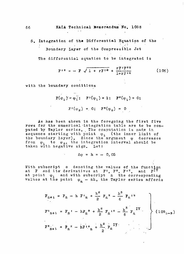
66 NACA Technical Mem~randurn’Nb’, 1058..

50 integration of tha Differential Equation of the,3’

Boundary Layer of the Compressible Jet,-

The differential equation to be integrated is

(106)

with the boundary conditions

I?I((C2)= o; F“(q2) = 0

As has been shown in the foregoing the first fiverows for the numerical “integration table are to be com-puted by Taylor series. The computation is made insequence starting with p“oint cpl (the inner limit ofthe %oundary layer). Since the argument q decreases

from 91 to ~2~ the integration interval should betaken with negative sign. Let :

Aq=h=– O.05

.With subscript o denoting the values of the functionat F and its derivatives at F~, I?ll,Fill, and ~IVat point VI and with subscript n the correspondingvalues at the point q -- nh, the Taylor series affords

n

1? =l’n-hrln+$h~

n+ IFrill_ _ Fnl!l

6‘.

~“1 = ~nl~2 IV

n+ 1 -hFnn +77n111–$Fn ~

1

(lo91_3)

2-~11.’ = an n - hy”lll

Iy” ’”’

n+ 1 ~+~.rn . . .,2 ,. ..

——.

. . NACA Technical ~~em.oqandurnNo.;,1058. .

Moreover. the differential -equation gi-v.es .., ..-

.-itnn+l = -’ ~n+lJ 1 + rF~an+l

ancl by further differentiating,

# rl?fl~+l+2YFIn+l F11n+lF111n+1= ———.-—— ——..— ------

n+l —1 -i-.rF!an+l “

,,-.

67

rF I

+ .—Q+l~’’2Q*&(1094)

l+rl?la n+ 1

2r2Jj’12 n+lF113n+l

- —--— .—.——- ——

(l+ Y?Yr2n+i)2

rF ~! Fllf

——-_—_ ---n+~ n+1 n+l. —— ——- ————— — F1

Jn+l 1 + rF12—————.———— n+ 1 (1095)

1 + rl?12 ..n-t-1

The .differentiation “is limited to the fourth derivative‘.In order to avoid the very complicated expression forthe fifth derivative. Computations show that the accuracythus obtained is entirely satisfactory-

The procedure of the preliminary computations isas follows. The boundary conditions give:

With a given value of VI for given value of the param–eter r

yt”n(vl) and F lV (q.)

are computed, Then by means of (1071_3) and (109/_5)

the values of F, F!, Fn, Ftn, and FIV at a neighbor-ing (second) point (ql - h) are obtained by (107) and(109). The same procedure is. follow&d for all fiv

& arein.itial’’points up to (CPl- 4h). The values ofrequired onlF~vuP to point 30 In the remaining rows ofthe table is not required (for the Adams method).BY denoting the linear increment of the function 1? and

I I1111111111111111111111111111II

68 NACA Tec-linfcal &,emor”andum’No. 1058

its first two derivatives Fl, S?ir”by T =’ hF~n;

Cn = hFlln; Vn = hFnln tables are constructed of

the linear increments of the functions and theirdifferences for the computed five points, The. tablesof tiifferences” a-re computed %y the fornulas given insection 4:

A4nn_4 = qn–4qn_l+6~n a-41’)n_3+ nn_4

These formulas are also used for the differences t, ~,whei-e, however

from the Adams series furthermore:

follow the increments in the function and its derivativesat the sixth, seventh, and so forth, points:

.. .

I

“NAC.A Technical J’iernorandum-No.j’.1058 69

each time increasing the computation table by one row.T~le calculation is .brok.en.oflf..”whenfor a given initial

:a;:;n;f 91 there is obtained at the-end of the table

V2 satisfying simultaneously the two boundaryconditions at the outer limit of the boundary layer:

FI(CP2,) = 0; l?ll(cp2)= o

If one of the derivatives becomes zero ahead of theother it indicates that the initial val,ue of. ql ,.was.not we’ll chosen.’ ‘.in this case it is necessary to- ‘ “recompute the table, ass,uming a new value of cpl, andso forth, until a successful result is obtained. Thecomputations carried out show that usually three tofour, approximations are sufficient to obtain an accurateintegral table for a given value of Bac

In the present paper the computations were carriedout for air (K = 1.41) first for Ba = 1, Subsequently,for the other values of Ba, it was possible to obtaina good result in a smaller number of trials by interpo-lation between the known resul’ts for Ba = 1 and Ba - 0(the latter corresponds to the solution of Tollmien whichgives the extreme values 91 = 0.981 and 92 = –2.04).

By this method of integration the final tables V,VI, and VTI were obtained for the values of the functionF and its derivatives Fl, Ffl, and F1!!, correspondingto various values of the argument Table V was obtaii~edfor Bao = 1.0 (VI = 0*923;:v2 = –9;.04); tabl’e VI forBao = 0.9 (V1 = 0.935; 02 = -2.04); table VII for Bao= 0-5(ql = 0.968; cpa = -2.04), l~Joreover,for comparison thereis presented table VIII in which the same magnitudes aregiven for Bao - 0 (Tollmien solution), that is, for thecase of an incompressible fluid.

Tables V to VIII include also a number of auxiliarymagnitudes

(CpTl - r F12

?:; cfF f _ y; __-___-; —-.U K ) ,.

by which the longitudinal and transverse velocity com-jjonents, velocity heads, and so forth, can be computed:

,., , . -. ., , .,


.,

6. Fundamental ,Properties of the Turbulent Boundary Layer,.

in the Plane—Parallel I?low of a Compressible Gas.-,-

The foregoing solution of the differential equationof the boundary. layer of a compressible gas jet makes itpossible to estimate the effect of the compressibility ona turbulent jet of high velocity

.,

(a) Geometry of the High-Velocity Jet

As is seen from the tables of numerical integrationthe effect of the compressibility is first of all todecrease the thickness of the boundary layer (region ofmixing of the jet with the surrounding fluid) with in—creasing flow velocity: that is; the coordinate 91of the boundary of the constant velocity core-(u = U6)decreases with increase in 3A, In particular for air(K = 1s41) the following values of ql for variousvalues of Ba are obtained: .

.Bao = 1 V1

= ,09923

Bao.~ (),9 . “

Bao = 0.5 cpl =0.966

Ba - 0 (incompress– 91 = 0.981ible fluid)

The relation between cpl and 3a in terms of thefactor of compressibility:

= 2(K-[

K-1r 1) Bao2 1 + ~ Bao2

1(110)

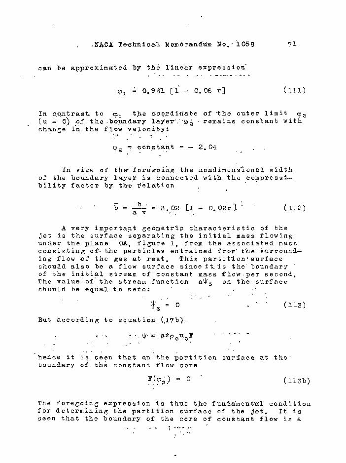
.NA.CA Technical Membranifum No. .‘1058 71

can be approximated by the linear expression”..- .----- -.,. . ------------

Vi = 0.981 [“i- 0.06 r] (111)

In cQnYrast ‘0 ‘% tthe ooo.rditiate of “the’outer limit qz,(U= O) of the .ho,undary layer’.”q~ J remains constant with

change i-nthe flow velocity:,,A>. .: .!.-

= constant = - 2.04Va - .. ,.’.“

In view of tlie’’’for~goingthe nondimensional widthof the boundary layer is connected wit,h the compressi—bility factor by the iblation , ‘ .

,.’ ~ = ~b:” = 3.02 [1 - 0.02r ].’”.,

(112)

A very important .geometr”i~ characteristic of thejet is the surface separating the initial mass flowingunder the plane OA, figure 1, from the associated massconsisting of. the particles entrained from” the ‘s’tiiround—ing flow of the gas at rest. This par.tit’ion:surfaceshould also be a flow surface since it,’is the” boundary ‘of the in;tial stream of constant mass flow.per second,The valuq o; the ~tream function a$~ on the surfaceshou~d be equal to zero:

.,,. .

. (113)

But according to equation (,17h)

“.$’= axpouoy ‘ . “‘ “.:. .,

.!,. .’

,..,-.

hence it is seen that o,n:the partition surface at the’boundary of the constant flow core

mp3) = o - (l13b),-,

The foregoing expression is thus t,he f.unda’mental conditionfor determining the partition surface of the jet, It isseen that the boundary o,f.the core of constant flow is a

. . .. ., i ‘-”- “’J’j -“

.

72 . NAC.A Technical Memorandum No? 1058

plane the position of which is determined by the valueof the nondirnensiona~ coo~d~nate

93 [~] ‘Q(o) (113C)

The integration tables in which the values of -F(@ aregiven afford, by inter~olati~ , the correspond&~ ~ues;

Ba=l V3 = - oo~os

Ba = 0,9 93 = - 0.200

Ba = 0,5 ~ = - 0,192.3

Ban+ O (incompress- cp = - 0,185ible fluid) -3

It is interesting ’to note that the relation between

Y3 and r is also linear.:

V3=-. 0.185 [1- 0,11 r~ (114)

Moreoveri. it has been show: that in contrast to theboundary- layer width which -decreases with increase inthe flow velocity, the widt,h of the core of c~nst’antmass flow increases with increase in velocity, Thelatter effect is explained by the deformation of theprofile of velocity heads in the boundary layer due tothe effect of the compressibility of the gtis at high flowvelocities,

(b) Vel~city Profiles

Tor greater clearfiess in comparing the velocityfields obtained for various values of Ba it is necessaryto choose an absolute (independent of Ba) system of co-ordinates. Lay off on the axis of ordinates:

and on the axis of abscissas!.,.

~?FI ~ -~:=; ~ = ~

Pouo Uo

.

.

. ..,. .. ..-

‘NACA Technical Memokandurn No. 1058 - 73

Then for’ all values o’f “Ba the’ values of ‘the coordinateson the inner (~1 = 1) and outer (?2 = O) ‘limits of theboundary layer are the ,same, regardless of the fact thatthe true coordinate of the inner limit cpl changes withchange in Ba,

Figure ~ gives the curves’ F!, I’f/K for Ba = 1along with the curve FI corresponding to the incompress-ible fluid (K = 1) forcomparison. As,rnay.le seen thevelocity- profile of the boundary layer becomes fullerwith increase” in the velocity in the undisturbed region(Ba = 1) while the’ PI profile becomes less full. Ingeneral, however, a weak effect of the compressibilityon the velocity profile of the jet is observed up toBa = 10

Figure 9 shows the same curves for Ba = 0.5, Thecharacter of the curves is the same but the effect ofthe compressibility is now so,weak that it may be practi–tally neglected.

I?igure 10 gives the densi’ty curves in the boundarylayer for Ba = 0@5 and Ba = 1.

Yigure 11 gives the velocity heads 1212/K for3a=l and Ba - 00

I’igure 12 shows a comparison of the transversevelocity component distribution:

.

for air at Ba = 1 ““‘ and for the incompressible fluid(!Collmien result),

(c) Rate of-l’low Discharge

As established in,,a previous “part of this paper thenondimensional rates of gas flow are subject to formula(75) which, applied to the entrained mass, gives ,

(115)

74 WACA Technical Memorandum No*- 1058

The nondimensional’magnitpde of the ini$ialmass in thejet is ..

Iiia =F1-t-a {116)

3

The integral tables ”give the values ‘F2(3ao) and Fl (Bao)and approximate integration of the values of the integrals

AZ =

2

fK’

()~FI--

-—~--dq)?Cp

3

1

for various values of Bao, Turther, assuming with Tollmiena= 0.C845 ; it is necessary to determine the magnitudesaAa, aAl and find the values of the entrained and initialmasses. (Computation shows that the values of aA2 andaA ~ are relatively very small.)

It is interesting to note that initial mass, entraiileclmass, and total mass flow through the boundary in theboundary layer of the plane-parallel flow of the high–velocity jet are linear functions of the compressibilityfactor:

(a) Initial mass:

G1 = 0.981 [1 - 0.06r]

(b) Entrained mass:

%2 = 0.389 [1 - O,lOr]

(117)

(118)

(c) Total mass rate of flow;

NA,CA Technical l~ie,morandurnNo. ‘1058 75

..? ,.

ml + mz = 1-!369C1– 0.07 r] - (li9)

., ..:- .,

In the particular case of an inc”ompressi’ble gas the con-ventional Tollmien values’ are:

FI1 =.0.981, ;2 = 0.388, ;1 + ;2 = 1.369

(d) Tractional Stresses

According to formula (93) the nondimensional ‘frictionalstresses at the boundary of the core of -constant mass flowis:

(1?f)bm, ‘7.--K3

3b—-——— +

ap !K’

3

() 12

t?;

——— d~ (120)&Q

With the use of the available integral tables the magnitudescorresponding to the various values of the compressibilityfactor r are obtained by the trapezoidal method. It isinteresting to note that for the stresses also a linearrelation, obtains:

T3- = y--——- --

2 3 = 0.27 [1 – 0i167 rJ “ (121)Uo

apo -T

where * 0.27 = ~~o is the nondimensional value of thefrictional stress in the incompressible .fluido

(e) Conclusions with Regard to the High Velocity Jet

The laws of variation of th,e fundamental propertiesof the turbulent boundary ‘layer of aplane-parallel streamof compressible gas (air) at high flow velocities havebeen obtained in the foreg~inga As in the case of the‘Iheatedlljet’ the most” int’kresting result obtained wasthat the effect of the compressibility on the fundamentalproperties of the high-velocity jet is negligible, This

.—

76 NACA !llechmical 1~,emorandtim. No, 1058

conclusion is valid UP to flow velocities attainingthe velocity of sound. (Y3a = 1)0 , .

In particular, on passing from small values of theBairstow number (B,a - 0) to Ba = 1, the angl”e of di- ‘vergence of the boundary la~yer riecreases by ‘2 percent;the angle of dissolution of the core of constant massflow increases by 11 percent; the nondimensional magni-tude of the entrained. mass ,de.cr.easesby 10 percent; thenondimensional magnitude of the initial mass decreasesby 6 percent; and lastly the nondimension.al value of thefrictional stress at the bcundary of the core of constantmass flow decreases by 1647 percent. The effect of thecompressibility onthe properties of the jet is ‘so smallthat at Fa = 0.5 it may be entirely neglected withoutimpairment of the results, hence that dynamic similarityof tile stream prevails over a very wide range of variationof the Reynolds num’her, the temperature above the s-arround-ings and of Ba. The second result in order Of ifiaoTtanceis that the variation of the fundamental properties witilr is linear. where r is assumed as the compressibilityfactor

[

k-lr.= 4 ~--—~ ;aoz 1 + — $ao2

2 2 1(122)

and only the outer boundary of the jet remains unchanged.

V, POSSIBILITY 03’DIRECT APPLICATION 03’THE

PRAYDTL LAW OF TURBULENT FRICTION T’O

THE CASE OF COIV,PRESSIBLE JET

. .In sect’ion I of the present investigation there was

obtained, for the free jet of compressible gas, the fric-tion law

~123)

which ’in those cases” whe”r~ the compressibility-may beneglected (p = constant) reduces to the known ~randtllaw Obtaified f~r incompressible gas:

.

N.AC6A..Technical Memorandum l~o.”ilU058 77

L,.“_, . . . . .

. .

. . (124)

.In comparing equations (123) and (124) t-he ~uestionnaturally ar~ises’“as,to what extent t-he ackyiracy. of thecompressible flow investigation is improved by introducingthe new friction law and whether this does not lead toa considerable complication of the problem. Since thesolption of the problem of the boundary layer of a high .velocity jet was obtained by the new friction law (123,)it remains to be explained whether it is possible with-out introducing large errors to simplify the given problemby direct application of the Prandtl friction law (124).BY the latter the differential equation of notion in the caseof free turbulence is written as follows:

(125)

.,

Setting, as previouslytassumed:

the differential equation is transformed to

...

.... . , . . .. , .’

3’

(126)

The differential equation in final form for boundary layerof a two-dimensional free jet then is:

II

78 NACA ?eclinical Memorandum Nop 1058

(127)

As may he -seen, the previous equation obtained by theapplication of the pran~tl friction law is considerably,more complicated than equation (20) which was obtainedon the basis of friction law (123) derived specially forfree jets of a compressible gas. In the case of largevelocities, as shown in section 111, a density distri-bution is obtained for which

Kt.- =K

K “=

-i-

( 128a)

(12ab)

Substitution of the foregoing equations in equation(127) leads to the following f~rm of differential equa-tioil of tke ~ouniiary layer of a free high-velocity jet:

,--—---- --

Oorfi.parisvnof the foregoing equation with the correspond-ing equation (105) gives

obtained with the improved friction law (123) shows con-elusively that the direct extension of the Prandtl fric-tion law to the compressible case not only fails to sim-plify the study of the latter but on the contrary givesa solution considerably more cumbersome than the ohe ob-tained by the more accurate friction law. In view of the -fact, however! that for a number of aerodynamic problemsof a compressible gas it may be more convenient to use

. IUCA Technical Memorandum Noo’ 1058.,... -..

79

the .f.r.i-ct=i-o-nclaw -i-nt:he-Prarrdt1--form,it wa-s-c-ensider eduseful for. solving equation (’129),by the Adams methodand compar-ing the results with “the solution of equation(106). - ,’

-i.The follawing results were obtained:

8(a) The qualitative ’results of the two soiutions -

of the problem are the same (with increasing velocitythe nondimensional values of the frictional” stressesdecrease, the width of the boundary layer decreases,the ve,locity field is slightly de$ormed, and the widthof the core of con’stant mass flow increases.

(b) The quantitative results of the two solutionsdiffer negligibly, Particular’lyby the use of thePra.ndtl frict’ion law (equation 129) it is found thatwith increase in the Bairstow number from Bao A O toBa=i ,the nondimensional frictional stresses decreaseby015 percent; the boundary layer thickness decreases by1.3 percent; the divergence angle of the core of constantmass flow increases 3Y 16 percent. Correspondingly with\he improved friction law (equation (106)) the nondimen-sional friction force decreased by 17 percent, the bound—ary layer thickness &ecr.sased by 2 percent, and. the di-vergence angle of the constant mass flow core increasedby 9 percents

The application “‘of t!le friction law of the incom-pressible fluid to the compressible flow thus .lea-ds toresults that differ s-lightly from the results ,obtainedwith the use of the corrected friction law, In the caseof the free jet, however, it is of advantage to, applythe corrected friction law since it leads to less cumber–some . and more readily solvable equations,

GENERAL CONCLUSIONS

./In the present paper. the-theory of free, turbulence

and the two-dimensional free jet was extended to a com-.press-ib,~efluid. In constructing the theory the tur-bulence hypothesis of Taylor (vorti.city interchange) wasused in -preference to the Prandtl hypothesis (pomentuminterchange). ‘ This was done because the former w,as con-firmed by test results on the velocity and temperature

80 .NACA T,echn.ical memorandum Xa. 3.058

fislds whereas. the second, while lead$ng to the samevelocity fields as the first, strongly deviated fromthe experimentally obtained temperature fields.

The differential equation of motion (12) for thet,.~o-dimen~i~nal..free compressible jet leads, in theparticular case of an incompressible fluid, to the well- ~known equation of Pra.ndtl~Tollmien-Schlicht ing.

The boundary layer considered was that of an infi-nite. plane-parallel flow, An infinite flow of thiskind assures constancy of the bouadary conditions in ‘the flow dir~ction: (1) at the outer limit of theboundary layer the flow velocity is equal to zero(u = 0),,<2) at the inner limit the undisturbed flowis of constant velocity u = uo, The constancy of thebo~ilda~y conditions (of the velocities temperatures,densities) at the edges of the boundary layer justifiesthe assumption of aerodynamic similarity (similarity ofvzlocitya temperature-fields, etc.) at the various cross-sections of the flow, that is, the existence of absolutedistribution laws of temperatures, velocities, densities,frictional stresses, and so forth, as was the case withincampressitle fluids. The absolute differential equa-tion o.fmotion (20) obtained for the boundary layer ofan infinite stream is solved for the two cases;

(1) Jet whose ten,perature differs from that of thesurroundings and whose velocities are small in ctimparisonwith the velocity of sound (Ilas 0.5),

(2) Jet o,f high velocities (up to 3A = 1) the tem-perature of which is equal to that of the surroundings.

The first pase involved the effect of compressibilitydue to the difference in the temperatures inside and out-side the jet; the second case the effect of the compress–ibility due to the high flow velocities.

The fundamental conclusion derived from the resultsof the present investigation is that the effect of thecompressibility of the fluid on the laws of flow in thefree jet is sma3L, It is also of interest that a lower-ing in the temperature of the moving fluid bel’ow that ofthe surrounding medium produces fundamentally the sameeffect on the properties of the flpw independent ofwhether the lowering was brought about by a cooling of

NAC.A”Technical. heno~andurn No. 1058 81

the jet or by the conversion of the heat “into’kineticenergy associated with the large f=l:ow~’,%elocit-ie-s:

In particular: I

(a) The nondimensional stres-ses’obtai,ned in the airjet at moderate velocities and at a temperature belowthat of the surroundings by 60° C were the same as forthe jet with large velocit-ies at : Bao = 1.0 and havea stagnation temperature equal to that of the surround-ings, (At Ba = 1.0 the local temperature was lowerthan the stagnation temperature by about 60°.G;) “

,!., .’,(3) The-nondimensional vel~city fields in both’ cases

practically agree (fig- 13)s.,

(c) The angle?f divergence of the core of constantmass flow in both jets increases by the same amount ofapproximately lU percent as conpared with the “incompress-ible jste

:. .. .

Special .ccmpre=sibility factors are introduced forthe nonisothermal jet (S) and for “the ‘jet wit’h highvelocities (r) and all fundamental properties of theboundary layer were ex~ressed as linear functions of “ .th-ese factors-

The small effect of the compressibility of the fluidpermits the conclusion that the free j’et maintains its ‘dynaiflic similarity over a wide variation of Bairstownumber and temperature differences as well as for a widerange of values of the Reynolds number: I

The author has not undertaken the investigation ofjets esca~ing from openings cf finite diameter and ofwakes behind bodies in a compressible fluid. ‘In these “cases the construction of a theory is effective only atgreat distances from the nozzle (or body) where the vel:’oc~ty and temperature difference are relatively smallancl hence the effect of .compressibility practically,inappreciable though the study of this effect, involvesgreat difficulty. . . . ,.

---- .

In concluding, the author wishes to express histhanks to V. K. Soladkin for his practical a-ssistancein “the mathematical part of thils paper and’ to A. T.Cherniavsky, K. L. Kozlovsky, and L. 1. Orlov, who,

....,.! -------—.

83 NACA Technical Memorandum No. io5q

under the supervision of Solcdkin, car~i’ed out all thenumerical computations.

$Translation by S. Reiss,National Advisory Committeefor Aeron-autics.

REFERENCES

1.

2.

30

4.

5.

6.

m1.

8.

9.

10.

11.

12.

Tollnien, Walter: Berechnung turbulenter Aus3reitungs-vorg!inge. Z.f.a.k.k., Bd. 6, Heft 6, 1926, pp. 1–11.

Swain: On the Turbulent Wake behind a 3ody of Revolution.Proc. Roy. SOC. of London, 125 A, 1929, p. 64’7.

Schlichting, H.: ~ber das el)ene [email protected]. , Id. I, Heft 5, 1930. .

Kuethe, Arnold iu.: 19v2stigations of the Turbulentkixing Regions Yorned by Jets. Jour. of Applov~cch., 1935, Pp. 8’7-95.

Abramovich, G.: Investigation of the Flow in the OpeilJet of a Wind Tunnel. Pts. I and 11, CAHI Reps.223 and 236, 1935,

Abra~ovich, G.: On the Theory of a Free Air Jst andIts Application. CAHI Rep. 293, 1936.

Abramovich, Go: Computation of the Air Resistance ofa Train on the Open Track and in the Tunnel. CAHI1938.

1

I’age, A. , and Talkn-er, V. : Proc. Roye SOC. (A), 1~32, P.7C2:

Taylor$ ‘G. 1.: The Transport of Vorticity an?. Heatthrough a Fluid in Turbulent Motionm Proc. RoyeSot. o’f London, vol. 135 A, 1932, ppo 685–702.

Taylor, G. 1.: Phil. Trans. Roy. Sot. of Londcn, ser.A, Vol, 215, 1915.

Durand, W, F. : Aerodynamic Theory, Julius springer,(Berlin), 1935, vol. III, p. 163.

Ruden, p, : Turbulence Ausbreitungsvorg5nge in ~reistrchloDie Naturwissenshafto i~o. 21/23, 1933.

TABLE1.- AUXILIARYFUNGZIONSOF NONISOTHERM@JET. TABLEII.- JET FUNCTIONSFOR Ato = -60UC.

Q

0,99

0,90

0,80

0,70

O,tw

0,50

0,40

0,30

0,20

0,10

0

–0,10

–0,20

–0,30

–0,40

–0,50

–0,60

-0,70

–0,80

-0,90

–1,00

–1,10

–1,20

-1,20

–1,40

—1,E43

–},&

–1 ,70

–1,30

—1,S4)

–2SXI

–2,04

FO

0!9810

0,8933

0,3019

0,7021

0$080

0,5152

0,4271

0,3430

0,2619

0,1M8

0,1161

0,0508

–0,0099

–0,0647

–0,1145

-0,15W

–0,1995

4,2326

—0,2653

–0,’2912

–0,3134

-0,3322

–0,3468

–0,3535

-0,3631

–0,3750

–0,3797

–0,33?3

–0,3853

-0,3870

–0,3874

–Oi?w

FO’

1,CQCO

0,9977

0,9358

0,S57

0,9383

0,9054

0,8675

0,8261

0,7789

0,7316

0,6799

0,6297

0,5760

0,5252

0,4728

0,4235

0,3731

0,3280

0,2833

0,2421

0,2035

0,1664

0,1345

0,1062

o,ol?05

0,0587

0,0412

0,0270

0,0165

0,0104

0,C078

o

F<

o

0,0746

O,lm

0,2370

OJO1O

0,3580

0,4050

0,4430

0,47?XI

0,4770

0,5110

0,5190

0,5200

0,5120

0,4980

0,4800

0,4390

0,4340

0,4070

0,3770

0,34541

0,3120

0,2770

0,2370

0,2040

0,1670

0,1300

0,0X40

o,a557

0,0177

0,0043

0

3CiFs

–0,C08

–O,(MI2

0,019

0,044

0,079

07122

0,173

0,228

0,287

0,265

0,420

0,437

0,556

0,627

0,693

0,757

0,818

0,924

0,924

0,973

1,014

1,0-50

1,083

1,108

1,132

1J44

1,155

1,I61

1,163

1,171

, 1,178

1,181

3 ws

-0,037

–0,118

–0,213

4,204

–0,391

–0,466

+L531

–0,684

–0,629

–0,634

-0,684

-0,694

-0,693

–0,682

–O,txiz

+633

-0,595

–0,505

-0,5Q5

-0,450

-0,401

–0,345

+,291

-0,238

-0,196

-O,MO

–o,102

-0,068

–0,040

–0,024

-0,016

-0003

3w’T

0,977

0,%9

0,933

0,878

0,799

0,711

o,&!3

0,504

0,389

0,316

0,16

0,053

O,col

-0,C50

—0,174

-0,246

-0,313

–0,402

–0,402

-0,428

–0,442

-0,448

—0,437

—0,405

–0,376

–0,329

–0,269

–0,193

–0,117

-0,021

0

0

.

?

——

1,SY35

0,9

0,8

0,7

o,&

0,5

0,4

0,3

(J,?

0,1

0

-0,1

4,2

-0,3

-0,4

-0,5

-0,6

-0,7

-0,8

–0,9

–1,0

–1,1

–1,2

–1,3

–1,4

–1,5

–1,6

–1,7

–1,8

–1,9

–2,0

‘—2,0

F

1!035

0,8989

0,8025

0,7031

0,MKJ9

0,5180

0,4313

0,3486

0,2691

O,lwl

0,1264

0,0629

0LM39

—0,0496

–0,0979

–0,1403

–0,1788

–0,2125

—0,2422

–0,2670

-0,28@0

–0,3961

–0,3203

–0,3317

–0,3401

—0,3468

–0,3515

–0,3544

–0,3558

–0,3581

-0,3581

–0,3681

F

1,0

3,s951

3,9307

D,9595

D,9294

0,8945

D,8549

),81645

0,7635

0,7164

O,&xl

0,6129

0,5539

0,5082

0,4567

0,4034

0,3583

0,3143

0,2705

0,2308

0,1941

0,1575

0,1268

0,1001

0,0757

0,0552

0,0387

0,0254

0,0155

0,0081

0,C020

o

F“

o

W!?8s

),M36

1,2536

3,3207

0,3755

D,321XI

1,4554

0,4826

),4848

0,5149

),5203

D,5200

0,5098

D,4937

D,4739

D,4513

D,4251

D,3971

D,3664

D,3341

D,3il19

0,2662

0,2270

0,1947

0,1589

0,1234

0,0881

0,0528

0,0172

0

n

7.

1,0

),S939

),9866

),9793

),9721

),%50

),9579

),9W?I

),9439

),9369

),93

),9232

),9164

),9095

D,9030

D,8%3

),8898

),8832

D,8767

D,8702

D,2639

D,8575

D,8S12

0,8449

D,8387

0,8326

0,8264

0,8203

0,8143

0,8083

0,8024

O,wo

F’Y

1,0

1,0012

1,s%41

0,9793

0,9560

0,9270

0,8925

0,3535

0,8089

0,7646

0,7132

0,6639

0,6699

0,5587

0,5058

0,4557

0,4028

0,3559

0,3036

0,2653

0,2247

0,1837

0,14s0

0,1185

0,0902

O,ofw

0,0463

0,0310

O,olw

O,olcm

0,0025

0

o

–0,0040

-0,0179

-0,0315

–0,0523

–0,0708

–0,0892

-0,1051

-0,1164

–0,1244

–0,1264

–0,1242

–0,1156

–0,1028

–0,0848

–0,0639

-0,0362

–0,0075

0,0258

0,0593

0,0939

0,1329

0,16$1

0,2015

0,2349

0,2639

0,28%

0,3112

0,3279

0,3427

0,3341

0,3S31

———

pF’— F F,z

% T

— —

o 1,0

–0,W40 0,9s63

-0,0181 0,9750

-0,0322 0,9401

-0,0538 0,8885

-0,07340,8291

.-0,09320,7630

-0,11050,6927

-0,12330,6176

-0,13280,5478

–0,13590,4728

-0,13450,4C68

-0,12620,3410

-0,11300,2840

-0,03390,2310

-0,07130,1361

-0,04070,1443

-O,(H)850,1108

0,02940,0835

0,06810,0012

0,10870,0436

0J552 0,0289

0,19750,0169

0,23350,0118

0,26910,0068

0,31700,0037

0,%04 0,CK118

0,37940,CQ08

-0,40270,0003

0,42490,ooo1

0,44140,ooo1

0,44751 0

e

I

0,9754

0,9453

0,9153

0,8853

D,8549

D,8242

0,7934

D,7622

),724)5

1,6989

),6674

),6351

),6026

),5704

),5371

),5042

),4711

9,4375

),4035

0,3698

3,3353

D,W38

0,2657

D,2303

0,1958

D,1597

0,1237

0,0878

0,0513

0,0150

0

~.

Po(n0)

TABLE IV.- JET FUNCTIONS FOR At(j= 120°CTABLE III.- JET FUNCTIONS FOR At = 60°C.—-

F’

1,0

1,0

D,9903

0,9731

0,9469

0,9154

0,8787

0,8378

0,7917

0,7448

0,6938

0,6440

0,5900

0,5387

0,4864

0,4368

0,3850

0,3-392

0,2932

0,2512

0,2121

0,I730

0,1399

0,1108

0,0844

0,0615

0,0433

0,0285

0,0173

0,0109

0,0081

0

r’

o

0,0537

0,1398

0,2180

0,2837

0,3426

0,3918

0,432

0,4646

0,4702

0,5075

0,5179

0,52@3

0,5139

0,5018

0,4853

0,4662

0,4418

0,41,57

0,3863

0,354b

0,3217

0,2676

0,2283

0,1959

0,1741

0,1358

0,0973

0,0582

0,0182

0

0

7.

1,0

1,CYX37

1,0038

1,0159

1,0221

1,0284

1,0340

1,0409

1,C500

1,0537

1,0Lw3

1,0660

1,C730

1,0796

1,0861

1,C928

1,0994

1,1061

1,1130

1,1197

1,1265

1,1334

1,1403

1,1472

I,IM2

1,1613

1,1683

1,1755

1,1826

1,1892

1,1971

1,2000

‘x

—.

F’T

,0

),9952

),9781

),9524

),9174

),8784

),3351

),7835

),7330

),6872

0,6343

),5830

D,5291

D,4784

D,4277

0,3803

D,3320

0,2897

0,2480

o,2m3

0,1758

0,1419

0,1137

0,0891

0,C674

0,0480

0,0334

0,0217

0,0131

0,0081

fi.—

0,s$

0,9

0,8

0,7

0,6

0,6

0,4

0,3

0,2

0,1

0

-0,1

0,2

0,3

.0,4

.0,5

0,6

F

0,96

0,89WI

0,8016

0,7011

0,6064

0,5125

0,4235

0,W4

0,2562

0,I7s6

0,1075

0S!41I

-0,0212

–0,0776

–0,1290

-0,1743

–0,2155

–0,2516

–0,2836

-0,3106

–0,3334

–0.3532

–0,3688

0,3813

0,3W3

0,3981

0,4033

0,4064

0,4089

0,4106

0,41lx

0,4106

F.— p

x

o

0,0010

-0,0093

-0,0196

-0,375

-0,0533

-0,0696

-0,0837

-0,0932

–0,GS97

-0,1014

-0,0s$0

–0,0W2

–0,0778

–o,otwl

–0,0404

–0,0141

+0,0128

0,0440

0,0755

0,1077

0,1437

0,1762

0,2039

0,2362

0,2633

0,2860

0,3045

0,3193

0,3279

0,3294

0,34.2(

——~,z-

1,0

W964

),9712

D,9321

9,8772

3,8149

3,7467

0,6743

0,5970

0,52M

0,4542

0,3392

0,3244

0,2688

0,2178

0,1746

0,1348

0,1041

0,0773

0,0564

0,0399

0,0264

0,0172

0,0107

0,0062

0,0333

0,0016

0,01Y27

0,CQ03

:’w ‘0,0001

0

e

—

,,0

),9781

),9416

),sOm

),8703

),832

),84)27

),7642

),7143

),6944

),6604

),6285

),5918

),5577

1,5244

3,4904

3,4573

9,4245

0,3908

D,3586

0,326?

0,2937

0,2617

0,2302

0,I934

0,1666

0,1356

0,1M2

0,0736

0,0449

0,0121

0

—

T

—

),942

0,9

0,8

0,7

0,6

0,5

0,4

0,3

0,2

0,1

0

-0,1

-0,2

–0,3

–0,4

–0,5

-0,6

-0,7

–0,8

–0,9

–1,0

–1,1

–1,2

–1,3

-1,4

-1,5

-1,6

-1,7

-1,8

-1,9

-2,0

-2,0

F F’F’——x

1,0

0,9963

0,93Q7

0,9579

0,9264

0,8901

0,8498

o,&K149

0,7540

0,7068

0,6545

0,6041

0,5499

0,49s0

0,4478

0,3997

0,3502

0,3067

0,2634

0,2244

0,1883

0,1526

0,1227

0,0966

0,0732

0,0530

0,0370

0,0242

0,0146

F’-F

0,942

0,8991

0,3013

0,7034

0,6051

0,6105

0,4206

0,3345

0,2513

0,1734,

0,1004

0,0328

–0,0306

– 0,0883

–0,1408

–0,1871,

1,0

1,0

D,9939

0,9783

0,9535

I

o 0 1,0

0,0009 0,0009 0,9952

-0,W62 –O,cw 0,9721

-0,0156–0,0162 0,9318

-0,0330-0,0318 0,8748

-0,0489–0,046s 0,8111

-0,0655–0,0616 0,7413

-0,0302–0,0746 0,6634

-0,0908–0,0835 0,5921

-0,0978–0,0889 0,5192

--0,1004—0,0903 0,4474

-0,G984–0,0375 0,3824

-0,0898–0,0789 0,3140

–O,0767 –0,0367 0,2632

I,0

D,9334

D,9442

0,9073

0,6677

0

0,0336

0,1253

0,2044

0,2713

0,3316

0,3824

0,4243

0,4586

0,4652

0,5051

0,5170

o,5m

0,5153

0,5645

0,i891

0,4707

0,4474

o,42m

,0

,0043

,0162

1,0272

0

0,001

-o,o#4

0,019s

-0,0333

-0,0548

-0,072C

-0,0871

–0,097!

-0,1051

–0,107:

–0,1055

–0,096[

–0,084(

-0,065(

–0,0441

–0,015:

0,0142

O,ow

0,034:

0,121:

1,0393

0,9233 1,0511

0,7926

o,755t

0,7190

0,6631

0,M73

0,6117

0,577C

0,5424

0,5032

o,474~

0,44I:

0,408:

0,37s

0,343:

0,311:

0,2771

0,247;

,0,217

0,187

0,157

0,127

0,097

O,O&l

0,039

0,011

0

0,84377

0,8477

0,8024

0,7556

0,7054

0,6358

0,6018

0,5503

0,4976

0,4475

I,0630

[,0751

1,0873

I,0996

1,1121

1,1248

1,1375

1,1504

1,1635

1,1767

l,lW

l,m35

1,2172

1,2310

1,2450

1,2600

1,2740

–0,0582~–O,OW~ 0,2128

–0,0367

–0,0377

0,0224

0,0579

0,0242

0,1318

0,1743

0,2134

0,25,10

0,2872

0;3217

o,351E

0,375[

0,3964

0,40M

0,413

0,430:

–0,0312 0,1702

–0,0065 0,1312

0,0186 0,1010

0,0476 0,0748

0,0765 0,0544

0,1059 0,0385

0,1383 0,0254

0,1675 0,0165

0,1949 0,0102

0,2205 0,0059

0,2415 0,0031

0,2604 0,0015

0,2758 0,W07

0,2878 00002

0,2933 O,wol

0,2955 0,0301

0,32800

–0,229410,3951

- 0,7

0,8

1–0,9

:–1,0

L,,,

–1,2

–1,3”

—1,4

—1,5

—1,6

–1,7

—1,8

I–1,9

--2,0

–2,04

–0,2664

-0,2993

-0,3272

–0,3507

–0,371C

–0,3372

–0,4002

–0,4101

– 0,4175

–0,4229

–0,4261

–0,4290

-0,4305

–0,4305

–0,4305

0,3486

0,3018

0,2539

0,2189

0,1733

,0,]446

0,1148

0,0878

0,0639

0,0450

0,029s

0,0180

0,0113

0,0084

0

D,3614

0,3287

0,2932

O,25XI

D,2180

0,1792

0,1400

0,1C04

0,0601

0,0185

0

0.

0,162!

0,200!

0,237[

0,272(

0,30s

0,3341

0,3W

0,377(

0,389!

0,394;

0,410(

1,2830

1,3320

1,3474

1,3627

1,3782

1,3938

1,4000

1.4003

0,0Q92

0,0068

0

0,0C60

o

}

iTABIIE*.- BABICFUNCTIONSFOR B% = 1.0.

—Mnln ‘? F P F’ F,,,

—

o 0,223 o,2x4000 1,OolxMo o —1,2922061 0,873 0,873027 0,993414 0,032W3 —1,2193542 0,823 0,823210 0,993778 0,121!341 —l,1417a53 0,773 0,773697 0,93W78 0,1770264 0,723

—1,C605300,724626 0,976143 0,228006 –0,977252

5 0,673 0,676124 0,963557 0,274762 –0,89’29156 0,623 0,628308 0,948737 0,317299- –0,8086507 0,573 o,5612e5 0,931895 0,35M43 –0,7254338 0,623 0,535149 0,913241 0,339675 —0,6440999 0,473 0,489937 0,892973 0,42W6 -0,5W36510 0,423 0,445873 0,871294 0,44646311 0,373 0,402878

–0,4897970,84838 0,4691S8 4,417885

12 0,323 0,361055 0,824433 0,488317 –0,34993113 0,273 o,3m447 0,799612 0,504203 –0,28615814 0,223 0,281103 0,774070 o,517a)415 0,173

–0,2267100,243049 o,747mo

160,526947

0,123-4,171613

o,m631317

0,721421 0,5342?70,073

—0,1203420,170912 0,694578 0,539099

18—0,074289

0,023 0,136659 0,667548 0,54173419 –0,027

–0,0318100,1041600,840437 0,542346

20 –0,077+o,om7@3

0,0728130,61334621 –0,127

0,5411150,042824

0,0417210,58~ 0,5W226

22 –0,1770,073216

0,0141730,55954923 –0,227

o,533a45 0,101545–0,0131369,532m3 0,528120 0,126950

24 -0,2774,039131 0,50675625 -0,327

0,521191 0,149703–0,~817 0,4@I1891 0,513191 0,170042

26 –0,377–0,0372270,455451 0,504225 0,1882m27 --0,427–0,1093730,430182 0,494401 0,20446228 –0,477–0,130284o,4mo’m 0}483803 0,2189852Y –0,527–0,1499850,382111 0,472528 0,23198930 –0,577-o,lMW 0,358778 0,460632 0,24365731” –0,677–0,2021220,313971 0,435229 0,26362932 —0,777—0,2313860,271793. 0,40802433

0,28CN)12–0,877—0,2565720,23?417 0,379320

34 –0,9370,293660

–0,2779700,195973 0,349363 0,3)519435 —1,077–0,2956720,1625E12 0,318342 0,315029w —1,177–0,3105930,132336 0.2&%07 0,32344237 —1,277 —0,3224470,105324 0,253693* –1,377

0,3M596-0,3317640,081618 0,220329

wo#336m3

—1,477-0,3338840,031276 0,18641740 –1,577

0,341531–0,8441350,044348 o,15m59 0,345442

41 —],677–0,3476680,030877 0,11736il42 –1,777

0,848~—0,3504280,0208W 0,0823% 0,30637

43 —1,877–0,3521590,014402 0,04725444 –1,977–0,3534360,011440

0,3522250,011970 —

45 –2,04 –O,wmo o 0 —

—N

nli

—

(

(

[

{

1(

II

12

13

14

15

16

17

18

19

20

21

22

23

24

25

26

27

28

29

TABLE.V(-a).-‘~ILIARf ltJliOTIONSFOR Bao= 1.0.

?

0,s23

0,823

0,723

0,623

0,523

0,423

0,323

0,223

0,123

0,023

–0,077

–0,177

—0,277

–0,377

—0,477

–0,577

–0,677

—0,777

–0,877

–0,977

–1,077

–1,177

–1,’277

—1 ,377

—1,477

–1 ,577

—1,677

— 1,777

–1,877

– 1,977

–2,04

%

1,Cm

0,9932

0,W32

0,9836

0,9758

0,%45

0,9523

0,9396

0,9?69

0,9145

0,9028

0,8918

0,3619

0,8729

0,2651

0,8567

0,8526

0,8479

0,6440

0,E409

0,8386

0,8368

0,8355

0,8347

0,8341

0,8337

0,8334

0,8334

0,8334

0,6340

0,8340

I

1,00

0,9@J38

0,9358

O,W-4

0,7783

0,7299

0,6793

0,6274

0,5747

0,5217

0,46’33

0,4188

0,3682

0,3205

0,2754

0,2331

0,1939

0,1581

0,1260

0,09778

0,07346

0,025M

0,01728

0,01370

0

@-F

o

-0,C05881

–0,018375

–0,037245

-0,077316

–0,094762

–0,108485

–0,117578

—0,121505

–0,HO041

–0,113213

—0,101240

–0,084478

–0,063388

–0,010436

+0,020203

0,052742

0,086504

0,[20771

0,154834

0,187948

0,219376

0,248379

0,274198

0,2S6087

0,313315

0,325126

0,826030

0,321YX?3

o

-0,C4)5341

–0,012W4

–0,037789

–0,058951

–0,030162

–0,115459

-0,126851

–O,132865

–0,132965

—0,126949

–O,114796

–0,096779

–0,073272

–0,044950

--0,012240

+0,023827

0,CW49I

0,102871

0,144015

0,1854)31

0,224953

0,262820

0,297781

0,328893

0,355276

0,375948

0,3W134

0,39201XI

0,392000.

—_F,:

z-——

0,9s5317

0,946376

0,887141

0,913826

0,732153

0,647276

0,562993

0,482403

0,33S627

0,279218

0,226474

0,181071

0,142613

0,110276

0,062635

0,045591

0,032?95

0,022167

0,014655

0,CQ9268

0,005560

0,003132

0,031640

0,060172

O,ml M

o

M[,II

o1234567PI9101112131415161718192021222324252627282930313233343536373839404142434445

TABLE VI.- BASIC FUNCTIONS FOR B% = 0.9._——

?.—

0,9340,8840,8340,7840,7340,6840,6340,5840,5340,4340,4340,3840,3340,2840,2340,1840,1340,0340,034

–0,016–’0,066–0,116–0,166–0,216–0,266--0,316–0,24%–0,416–0,466–0,516–0,566–0,666–0,766–0,866–0,966–1,066–1,166–1,266—1,366— 1,466—1S66– 1,666—l,76b—1 ,866—1,966–2,04

F

0,9340000,8340260,8342010,72466s0,7335580,6869960,6390900,5919500,5456640,5003220,4559930,4127510,3706470,3297320,2900480,2516320,2I45040,1786950,1442120,1107200.0792710,0438230,019703

–0,033067–0,034525–0,059671–0,083531—0,106113–0,127454—0,147566-0,166480–0,203330—0,230735–0,256465–0,278298–0,296528–0,311461–0,3234184,332721– 0,339710–0,344717–0,348088–0,350173—0,351319–0,351876–o,3520fM

F’

1,000,S934820,9940420,9363620,9771300,9650370,9507300,9345500,9165380,8969330,8759190,8526630,8203440,3061120,7811220,7294180,7294130,7029590,6762490,6493930,6224830,5956160,5638560,5422960,5159820,48S$920,4643670,4391620,4144220,39018s0,3664890,3203460,2777330,2372310,1998090,1652980,1339150,1057500,0808920,0593980,0-413210,0267050,0155680,0079350,CK13220

o

F’‘

o0,0601760,1168180,1697620,2188950,2641520,3065260,3430440,37677I0,4068010,4332550,4562830,4760380,4926950,5064430,5259380,5259380,5320530,5360070,5379570,538C690,5365100,5334260,528951o,5~3218

0,5163430,5084330,4996910,4899030,47944I0,4882860,4441280,4178720,3898620,3603750,3296490,2978760,2652320,2318610,1979180,1635240,1288020,0938590,0587650,023606

0

F,,,

— 1,236624—1,168140– 1,095812— I,0207I1– 0,943871–0,866263–0,788765–0,712178–0,637192– 0,56440I–o,494mo–0,427252–0,363573–0,303458–0,247031–0,1463W–0,145390–0,100106–0,058384_13,0q@331j

+0,0149580,0469220,0760260,1024540,1264300,1431490,1678230,1856270,2017640,2163850,2296550,2526950,27!8540,287%40,3014200,3128160,3223350,3303320,2367990,341!X180,3457690,3485950,3303030,3513480,351830

—

o

1

2

3

4

5

6

7

8

9

10

11

12

13

14

15

16

17

18

19

20

21

22

23

24

25

26

27

28

29

30

TABLE VI(a).- AUXILIARY FUNCTIONS FOR B% = 0.9.—..

‘?

.—

0,934

0,834

0,734

0,634

0,534

0,434

0,334

0,234

0,134

0,034

—0,CH36

–0,166

–0,266

–0,366

–0,466

–0,566

–0,666

–0,766

– 0,866

–0,966

— 1,066

–1,166

—1,266

– 1,366

—1 ,466

–1,566

– 1,666

--1,766

—1,866

—1,966

-2,040

%

1,00

0,9385

0,9944

o,9a31

0,9801

0,9708

0,9606

0,9501

0,9395

0,9292

0,9193

0,9102

0,9017

0,8942

0,3376

0,3318

0,8770

0,8789

0,3696

0,8670

0,3650

0,8635

0,8624

0,8616

0,3612

0,8609

0,3607

0,8606

0,8606

0,8MM

0,8606

i-T

.—

I ,00

0,9355

0,9826

0,9622

0,9351

0,9)23

0,8644

0,8221

0,7764

0,7278

0,6771

0,6250

0,5722

0,5193

0,4669

0,41s6

0,3658

0,3182

0,2729

0,2305

0,1911

0,1551

0,1226

0,09339

0,06897

0,04806

0,03103

0,01809

0,03922

0,00443

0

o

–0,005170

–0,018345

–0,026295

– 0,056233

–0,075344

–0,C93312

–0,107265

–0,116762

–0,121220

–0,120355

—0,114138

—0,102726

~—0,036427

–0,065667

–0,040953

–0,012853

+ 0,017992

0,050936

0,085283

0,120320

0,155316

0,189539

0,222223

0,252633

0,28CQ08

0,303598

0,322630

0,336512

0,34601XI

0,352000

0

—0,005178

–0,013448

–0,036732

–0,057375

-0,078125

–0,097139

–0,112899

–0,124231

– 0,130456

–0,130920

–O,125399

–O,113925

–0,096653

– 0,073933

–0,046443

–0,014656

+0,020621

0,058574

0,098366

0,139099

0,179868

0,219781

0,257919

0,293350

0,325250

0,352734

0,374943

o,39]om

0,4020LM

0,409000

F?T

1,Cmoo

0,9896

0,9602

0,9149

0,8571

0,7W3

0,7178

0,6422

0,5663

0,4922

0,4215

0,3555

0,2953

0,2412

0,1935

0,1523

0,1174

0,08837

0,06477

0,M605

0,03159

0,02077

0,01297

0,00759

0,00409

0,0)193

0,@3082

0,0C028

0,KKI07

o

0

-J

—Nn/n

—

o12345678910II12131415161718192021222324252627282930313233343336373839404142

4344

1TABLE vlI.- BASICFUNCTIONSFOR B% = 0.5.

‘f

0,%60,9160,3M0,8160,7660,7160,6660,6160,5660,5160,4660,4160,3660,3160,2660,2160,1660,1160,(%40,016

–0,034–0,034--0,134--0,184–(),234–0,284–0,334–0,384–0,434– 0,484–0,534– 0,634–0,734-0,834–0,934—1,034—1,134—1,234–1,334–1,4M–1,534—1,734—1,834—1 ,934–2.04

F

0,9660,9160220,8661730,8165750,7673430,7185360,6704030,6228890,5761290,5302050,4851880,4411430,3981320,3562020,3154090,2757840,2373710,2001950,1642770,1296460,0%3060,C642800,0335620.0041580,0239260,0507100,0761860,1003780,1232940,1449540,1653750,2025950,2351690,2633190,2873160,3274390,3239970,3373060,3477050,3555340,3611520,3671780,363320

O%K-QO

i-

1,00,9986950,9948710,9886720,9802410,9597220,9572600,9429950,9270770,9096340,8938160,8707410,8495510,8273600,W43LM0,780477O,756IM70,7310000,7055430,6?975I0,6537020,6274890,6011920,5748890,5486530,6225530,4965540,4710150,4456960,4207450,3962140,3486030,3231910,2622760,2201020,1828770,1487910,1179760,03CL5620,WW370,0462750,0164300,007CW0,001261

0

o0,051755o,m36950,1467760,1899730,2302820,2677100,3022390,3340590,363C640,3893LuI0,4130650,4342130,4528970,4692210,48327?0,495143“0,5049520,5127760,5127760,5223460,5253620,5262450,5256230,5235850,5202100,5155350,5097860,S28820,4949520,4850540,4656270,&20780,4158340,3873010,356818O,3247XI0,2313070,2368310,2215310,1Wi180,11%400,0753540,038998

0

—1,062600—1,006931–0,950190–0,892768–0,835025–0,777326–0,71W89—0,663311– 0,607562–0,552974–0,309746–0,448052–0,398029–0,349786–0,303412–0,258955—0,216460– 0,175936–0,137379–0,137379–0,066092–0,033293–0,0023160,0268390,0543790,08023)o,I044940,1272520,1485600,1684930,1371090,22%410,2496350,2745030,2956370,3133720,3280290,3398950,3492560,3563860,3615630,3672320,3683300,363702

—

—h!!

nr

—

(

1

2

~

4

5

6

7

8

9

10

11

12

13

14

15

16

17

18

19

20

21

22

23

24

25

?b

?7

28

29

30

TABLEVII(a).-AIJXILIARY~CTIONS’FOR BI——

?

——

0,966

0,366

0,766

0,666

0,566

0,466

0,366

0,266

0,166

0,066

–0,034

–0,134

–0,234

– 0,334

—0,434

–0,534

–0,634

4,734

–0,334

– 0,934

– 1,034

– 1,134

1,234

— I,334

– I,434

– 1,534

— 1,634

— I,734

– 1,834

— 1,934

–2,040

%

I,00

0,9996

0,9983

0,9363

0,9W

0,9903

0,9372

0,9838

0,9302

0,9767

0,9733

0,9702

0,9672

0,9642

0,s622

0,W13

0,9584

0,9570

0,9557

0,9549

0,954I

0,9535

0,9532

0,9528

0,9527

0,9525

0,9525

0,9524

0,9524

0,9524

0,9524

-

F’T

1,00

0,?954

0,9819

0,96C9

0,9331

0,8993

0.8607

0,8176

0,7713

0,7223

0,6717

0,6197

0,5672

0,5148

0,4632

0,4127

0,3637

0,3168

0,2724

0,2305

0,1917

0,1552

0,1238

0,0951

0,0659

0,0487

o,wm93

0,01720

0,00740

0,00140

0

o

-0,(04573.

-0,016643

-0,CL326W3

–0,051429

–0,07CX188

–0,037132

–0,101509

-–0,111871

—0,117677

-0,1W06

–0,114162

–0,104474

–0,089714

–0,070106

–0,046225

4,013405

-’-0,012669

0,046219

0,081716

0,113338

0,155297

0,191703

0,2.268115

0,21XI&34

0,2W52

0,316710

0&M778

0,3555’20

o,3w02

0,36$3

—

qP— Fz

o

-0,016571

–0,032925

--0,051760

-0,070775

–0,103181

–0,114131

–0,120434

–0,121757

–0,117668

–0,108017

4,072W

—0,048135

–0,019202

+0,013238

0,048361

0,035575

0,124031

(),162870

0,2011I8

0,238041

0,272944

0,304621

0,332504

0,355710

0,373289

0,334504

0,38750

=0.5.

l,OWO

0,9902

0,SR525

0,9197

0,3650

0,3013

0,7311

0,6575

0,5831

0,5097

0,43S0

0,3725

0,3112

0,2558

0,2064

0,1635

0,1268

O,OWJ

0,0706

0,0507

0,03542

0,0232

0,0146

0,CQ36

0,0046

0,CQ22

0,0303

0,0002

0,0000

0,0000

0

oPI-J

. .. —.—. — —

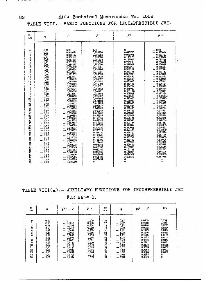
88 NACA Technical No. 1058

TABLE VII I.- BASIC FUNCTIONS FOR INCOMPRESSIBLE JET.

iNn,n

—.

o1

:45676

1:111213

;;161718

;;2122232425

%’28

%31323334353637383940414243 “444546

?

0,980,930,880,830,780,730,680,630,58(3,530,480,430,380,330,280,230,180,130,08

— 8:Y2— 0,07— 0,12- 0,17— 0,22--0,27— 0,32— 0,37— 0,42— 0,47

0,52— 0,62— 0,72— 0,82— 0,92– 1,02- 1,12— 1,22— 1,32— 1,42- 1,52— 1,62— 1,72-- 1,82— 1,92— 2,02— 2,04

—

F F’ Ff’

np47i&0;1357700,17E43620,2i38W0.2493090,2820190,2.129570,3412710,3672SU0,3910690,4126450,4320790,449414$::;;;

O:48942O0,4989480,S3M780,5126M0,5169890,5196660,5206440,520423g,:;:;:;

0:5113280,54)573Io,4989&l0,491134g,:wx~

0:4$44330,3961020,36$4260,3327890,332769O,26293I30,2264170,1890760,1511710,1128730,0743070,03557so0 —

TABLE VIII(a) .- AUXILIARY FUNCTIONS FOR INCOMPRESSIBLE JET

FOR Ba=O.

T’

0,920,680,780,680,5s0,480,380,280,18

— %%– 0,12— 0,22— 0,32— 0,42— 0,52

I

yF’ — F

- ICHM2— 0,0155— 0,0310— 0,0486— 0,0667— o,cEi35— 0.0378—o;lo&— 0,114/— 0,1162— 0,1126- 0,1037— 0,0898— 0,0708– 0,0474

J’&n,n ~ f’

;;18

u2122232A25262728

331

— 0,62– 0,72— 0,82— 0,92— 1,02– 1,12— 1,22– 1,32— 1,42— 132— 1,62— 1,72— 1,82- 1,92— 2,02— 2,04

yF’ — F

— 0,0203– O,o11o

0,04460,06030,11730,15460,19150,22720,26060,28110,31780,33980,33640,36660,36970,3690

F’2

o

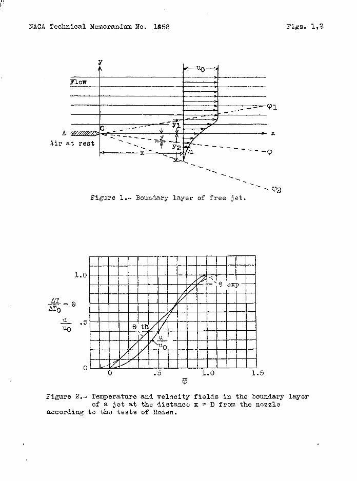
NACA Technical Memorandum No. 1058 Figs. 1,2

Flow‘ *-

——---t--+ --- V1---

0A~ *-_-.-’----

Air at rest =:’

F

-..‘\\

‘\‘.+

. C42

Figure 1.- Boundary layer of free jet.

1

AT=eATo

.0

.5

no

Figure 2.- Temperatureof a jet at

according to the tests

.5 1.0 1.5

@

and velocity fields in the boundarythe distance x = D from the nozzleof Rude~.

layer

,

IT “- -

NACA Technical

-.-. .-— ---- —

Memorandm No. 1058

1.0

Fr UK_= _-o

4

.5

0 .5

G1.0

Figure 3.. Velocity fields in theboundary layer of a

jet at various temperatures.

.

1*O

e .S

o ●5 1.0

Figure 5.- Temperature fields inths boundary layer

of a jet.

Figure 7.- Fields oftransverse

velocities in theboundary laysr of a jetat Pt = -60°c.

Pigs. 3,4,5,6,7

1.0

K.5

u .5 1.0@

Ff~re 4.- Density fields in thefree jet at At = +60°C

ani At = -600c.

.0

.5

lV..—a vo

o .5 1.0@

Figure 6.- Field.of velocity headsin the free jet at At=-GO°C.

.5

0

0 .5 1.0c?

..., . ,. , , ,,., , .. ..... . . .. ... .-.. ...-.-—-. —-—... -—..-. —.—.--——-— -——

,.

NACA Tecmlical Memorandum No. 1058 Figs. 8,9,10,11,12,13

0 .5 1.0Figure S.; Velocity fialds in

boundary layer of ahigh velocity jet (Bao = 1).

the

1.0

~1 .5

0 .5 1.0 ~FiLmre 9.- Velocity fields in the

boundary layer of ahigh velocity jet (Bao = 0.5).

1.0 I t 1

I 1.0

‘~ Ba.1

1?— -.-?.F _ ~l,_—-

K.5

R

.5

0 .5 1.0Figure 10.-

0 .5 1.0 F‘ensity ‘ie13s ‘n ‘~l” Figure 11.-%oundary laysr of a

Fields of velocity headsa high velocity jet.

high velocity jet.1.0

.5

I?I=L17-*— TUoa V. .5

0

0 .5 + 1*O o .5 @ 1“0I’iugre12.- Transverse velocity I’igure13.- Coi.lparisonof velocity

field in a high fields of I cooled d~$ ,vciocity jet. (At = 60°) and II jet with high

vdoc~tj,es (Bao = 1).

I ——. .,. ,. , , .,.-..!. -- . ..—— -------

technical memorandums - nasa · technical memorandums-1 natioitaladvisory 601vu41$t!eeror...

Documents