technical r eport treewidth-preserving modeling in asp

Technical

R e p o r t

Institut fur Informationssys-

teme

Abteilung Datenbanken und

Artificial Intelligence

Technische Universitat Wien

Favoritenstr. 9

A-1040 Vienna, Austria

Tel: +43-1-58801-18403

Fax: +43-1-58801-18493

[email protected]

www.dbai.tuwien.ac.at

Institut fur Informationssysteme

Abteilung Datenbanken und Artificial Intelligence

Treewidth-Preserving Modeling inASP

DBAI-TR-2016-97

Manuel Bichler Bernhard BliemMarius Moldovan Michael Morak

Stefan Woltran

DBAI Technical Report

2016

DBAI Technical Report

DBAI Technical Report DBAI-TR-2016-97, 2016

Treewidth-Preserving Modeling in ASP

Manuel Bichler 1 Bernhard Bliem 1

Marius Moldovan 1 Michael Morak 1

Stefan Woltran 1

Abstract. For ground ASP programs where an appropriate graph representationhas bounded treewidth, algorithms that exploit this bound on the treewidth theo-retically only require linear time for checking existence of an answer set. However,in practice such algorithms are hardly competitive against state-of-the-art CDCL-based solvers, which do not explicitly rely on bounded treewidth. In this work weinvestigate the hypothesis that CDCL-based solvers leverage small treewidth im-plicitly. We identify modeling constructs in non-ground ASP that significantly blowup the treewidth in the grounding and we give guidelines for modeling problems innon-ground ASP such that grounding preserves small treewidth of the input. Wealso experimentally show that a non-ground rule decomposition technique can de-crease the treewidth of the grounding substantially. Finally, we identify a class ofnon-ground ASP programs that preserves bounded treewidth in the sense that thetreewidth of the grounding only depends on the treewidth and the degree of theinput graph instead of its size.

1Institute for Information Systems 184/2, Technische Universitat Wien, Favoritenstrasse 9-11,1040 Vienna, Austria. E-mail: [bichler,bliem,moldovan,morak,woltran]@dbai.tuwien.ac.at

Acknowledgements: This work has been supported by the Austrian Science Fund(FWF): Y698, P25607.

Copyright c© 2016 by the authors

Technical Report DBAI-TR-2016-97 2

Contents

1 Introduction 3

2 Preliminaries 5

3 Empirical Investigation of Modeling Techniques 103.1 Encodings . . . . . . . . . . . . . . . . . . . . . . . . . . . . . . . . . . . . . 11

3.1.1 Hamiltonian Cycle . . . . . . . . . . . . . . . . . . . . . . . . . . . . 113.1.2 Secure Set . . . . . . . . . . . . . . . . . . . . . . . . . . . . . . . . . 133.1.3 Minimum Weighted Dominating Set . . . . . . . . . . . . . . . . . . . 14

3.2 Experiments . . . . . . . . . . . . . . . . . . . . . . . . . . . . . . . . . . . . 163.2.1 Hamiltonian Cycle . . . . . . . . . . . . . . . . . . . . . . . . . . . . 193.2.2 Secure Set . . . . . . . . . . . . . . . . . . . . . . . . . . . . . . . . . 223.2.3 Minimum Weighted Dominating Set . . . . . . . . . . . . . . . . . . . 22

3.3 Impact of Rule Decomposition . . . . . . . . . . . . . . . . . . . . . . . . . . 223.3.1 Experiment Setup . . . . . . . . . . . . . . . . . . . . . . . . . . . . . 233.3.2 Results . . . . . . . . . . . . . . . . . . . . . . . . . . . . . . . . . . . 243.3.3 Discussion . . . . . . . . . . . . . . . . . . . . . . . . . . . . . . . . . 26

4 Theoretical Investigation of Modeling Techniques 264.1 Modeling Techniques That Destroy Bounded Treewidth . . . . . . . . . . . . 264.2 A Treewidth-Preserving Class of Non-Ground ASP . . . . . . . . . . . . . . 28

5 Conclusion 33


1 Introduction

Answer Set Programming (ASP) [10, 20, 25, 28] is a well-established logic programmingparadigm based on the stable model semantics of logic programs. Its main strength is afully declarative language and the fact that, generally, each answer set of a given logic pro-gram directly describes a valid answer to the original question. Moreover, ASP solvers—see,e.g., [2, 3, 15, 24]—have made huge strides in efficiency and are increasingly used for indus-trial applications like planning or scheduling. A logic program usually consists of a set oflogical implications (called rules) and a set of facts. Deciding the consistency problem, thatis, whether a given disjunctive logic program has an answer set, is NExpTimeNP-completein the combined complexity, where both the rules and facts are treated as input, and Σ2

P-complete in the data complexity, where the set of rules is fixed; cf. [14].

In practice, when problems are modeled using the ASP logic programming language, theusual goal is to write a fixed program (i.e., set of rules) that solves the general problem. Theconcrete input is then supplied as a set of (ground) facts. The answer set solver takes the fixedprogram, plus the ground facts, and computes the answer sets, that is, the solutions to theoriginal problem, as described earlier. Logic programming in general, and ASP in particular,have gained popularity because of this intuitive, declarative way to solve problems and thestraightforward syntax. The following example illustrates this:

Example 1. For an input graph specified as vertex(.) and edge(.,.) facts, the followingprogram solves the three-colorability problem:

1 { col(V,red), col(V,blue), col(V,green) } 1 :- vertex(V).

:- edge(X,Y), col(X,C), col(Y,C).

The first rule guesses exactly one of three colors for each vertex, while the second rule makessure that no neighboring vertices have the same color.

Evaluating an ASP program is usually a two-step approach (all current state-of-the-artsolvers work in this way): First, the input program is grounded, that is, the variables in theprogram are replaced (in the worst case) by all possible, valid combinations of constants fromthe input domain. Secondly, a solver evaluates the (now) ground program, and computesthe answer sets. Note that the grounding step is exponential in general. The difficultyof solving ASP programs is then often determined by certain parameters of this groundinput program. Straightforward parameters include the size of the grounding, or the ratiobetween rules and atoms in the program. However, there are also more evolved, structuralparameters. One such parameter is the treewidth of the ground program. The groundprogram is converted to a graph representation, and, intuitively, the treewidth then measureshow close this graph is to a tree. It turns out that favorable theoretical runtime results canbe established if the treewidth is small. Several algorithms have been proposed [26, 31]and implemented [29], but, despite linear runtime in theory, they have generally turned outto be hardly competitive when compared to state-of-the-art answer set solvers like clasp for


consistency checking1. Furthermore, these algorithms are not designed to be general-purposesolvers, since they can only perform well on low-treewidth input programs. However, othersolvers, like clasp, perform well consistently on such low-treewidth inputs, but also performwell on other instances. This begs the question whether existing CDCL-based solvers areinherently sensitive to low treewidth ASP programs.

It is the aim of this report to investigate the impact of the treewidth of ground programson the runtime of existing state-of-the-art CDCL-based solvers. Our working hypothesis isthat the answer to this question is affirmative. However, ASP problem encodings are usuallywritten in non-ground form, in order to make use of the full, intuitive, and expressive ASPlanguage. The actual input instance, consisting of ground facts, is then combined withthe encoding, grounded, and then finally passed to the solver. Therefore, another interestingquestion arises: Assuming that the ground facts of the input instance, represented as a graph,already have low treewidth, which ASP language constructs may be used when writing theencoding, such that the low treewidth of the input instance is preserved in the groundedprogram? Furthermore, does the recently proposed approach of rule decomposition on thenon-ground program [5, 7, 30] have an influence on the treewidth of the ground programobtained from it? Having these questions in mind, our main contributions can be stated asfollows:

1. We perform an in-depth experimental investigation of different encodings for the samegraph problems in order to identify those encodings that best preserve the low treewidthof the input graph (represented as ground facts) in the ground program obtained fromcombining the input graph with the respective encoding. We show that constructslike transitivity lead to a dramatic increase in the treewidth, while constructs likereachability do not, and identify the reasons for this, formulating several overarchingguidelines for encoding problems in ASP in such a way that the treewidth of the inputinstance is preserved.

2. We investigate, via an experimental evaluation, the impact of a certain rewriting tech-nique (viz. rule decomposition of non-ground programs, cf. [6]) on the treewidth ofthe corresponding ground program, that is, we compare the original encoding with thedecomposed encoding for the same input graph. We show that this impact can besubstantial and often reduces the treewidth by a large amount.

3. We isolate a class of ASP programs with restricted syntax that guarantees that forany encoding in the class and for any input graph of bounded treewidth and boundeddegree, the treewidth of the corresponding ground program remains bounded as well.To be more precise, we showed that the treewidth and the degree of the groundedprogram only depends on the clique-width (a parameter more general than treewidth)and degree of the input graph. That is, for any non-ground ASP programs in this

1This, however, is another story for answer set counting, where these approaches prove to be highlycompetitive in some settings [17].


class, the treewidth of the grounded program does not depend on the size of the inputgraph.

The remainder of the paper is structured as follows. In the next section, we will intro-duce relevant background information regarding the ASP language and tree decompositions.Then, we report on our experimental evaluation regarding the impact of different encodingsand rewriting strategies on the treewidth of the grounding. Section 4 provides our theoreticalresults on classes of programs which show robust treewidth with respect to the groundingstep. In the final section, we conclude the paper with some observations and ideas for futurework.

2 Preliminaries

General Definitions. We define two pairwise disjoint countably infinite sets of symbols:a set C of constants and a set V of variables. Different constants represent different values(unique name assumption). By X we denote sequences (or, with slight notational abuse,sets) of variables X1, . . . , Xk with k > 0. For brevity, let [n] = {1, . . . , n}, for any integern > 1.

A (relational) schema S is a (finite) set of relational symbols (or predicates). We writep/n for the fact that p is an n-ary predicate. A term is a constant or variable. An atomicformula a over S (called S-atom) has the form p(t), where p ∈ S and t is a sequence ofterms. An S-literal is either an S-atom (i.e. a positive literal), or an S-atom preceded bythe negation symbol “¬” (i.e. a negative literal). For a literal `, we write dom(`) for the setof its terms, and var(`) for its variables. This notation naturally extends to sets of literals.For brevity, we will treat conjunctions of literals as sets. For a domain C ⊆ C, a (total ortwo-valued) S-interpretation I is a set of S-atoms containing only constants from C suchthat, for every S-atom p(a) ∈ I, p(a) is true, and otherwise false. When obvious from thecontext, we will omit the schema-prefix.

A substitution from a set of literals L to a set of literals L′ is a mapping s : C∪V→ C∪Vthat is defined on dom(L), is the identity on C, and p(t1, . . . , tn) ∈ L (resp. ¬p(t1, . . . , tn) ∈L) implies p(s(t1), . . . , s(tn)) ∈ L′ (resp., ¬p(s(t1), . . . , s(tn)) ∈ L′).

Answer Set Programming (ASP). A logic programming rule is a universally quantifiedreverse first-order implication of the form

H(X,Y)← B+(X,Y,Z,W) ∧ B−(X,Z),

where H (the head), resp. B+ (the positive body), is a disjunction, resp. conjunction, ofatoms, and B− (the negative body) is a conjunction of negative literals, each over terms fromC ∪V. For a rule π, let H (π), B+(π), and B−(π) denote the set of atoms occurring in thehead, the positive, and the negative body, respectively. Let B(π) = B+(π) ∪ B−(π). A ruleπ where H (π) = ∅ is called a constraint. Substitutions naturally extend to rules. We focus


on safe rules where every variable in the rule occurs in the positive body. A rule is calledground if all its terms are constants. The grounding of a rule π w.r.t. a domain C ⊆ C is theset of rules groundC(π) = {s(π) | s is a substitution, mapping var(π) to elements from C}.

A logic program Π is a finite set of logic programming rules. The schema of a programΠ, denoted sch(Π), is the set of predicates appearing in Π. We call a predicate intensionalin Π if it occurs in the head of a rule of Π, and we call it extensional otherwise. An atomis intensional or extensional whenever the involved predicate is. The active domain of Π,denoted adom(Π), with adom(Π) ⊆ C, is the set of constants appearing in Π. A program Πis ground if all its rules are ground. The grounding of a program Π is the ground programground(Π) =

⋃π∈Π groundadom(Π)(π). The (Gelfond-Lifschitz) reduct of a ground program Π

w.r.t. an interpretation I is the ground program ΠI = {H (π)← B+(π) | π ∈ Π,B−(π)∩ I =∅}.

A sch(Π)-interpretation I is a (classical) model of a ground program Π, denoted I � Πif, for every ground rule π ∈ Π, it holds that I ∩ B+(π) = ∅ or I ∩ (H (π) ∪ B−(π)) 6= ∅,that is, I satisfies π. I is a stable model (or answer set) of Π, denoted I �s Π if, inaddition, there is no J ⊂ I such that J � ΠI , that is, I is a subset-minimal model ofthe reduct ΠI . The set of answer sets of Π, denoted AS (Π), are defined as AS (Π) ={I | I is a sch(Π)-interpretation, and I �s Π}. For a non-ground program Π, we defineAS (Π) = AS (ground(Π)). When referring to the fact that a logic program is intended to beinterpreted under the answer set semantics, we often refer to it as an ASP program.

ASP Language Extensions. The ASP-Core-2 language specification for the standardizedASP language [11] defines several additional constructs to those discussed above, whichwe will briefly introduce here. Please see [11] for precise formal definitions of syntax andsemantics. We will call rules that do not contain any such extensions simple.

Arithmetic expressions are atoms of the form

X 4 ϕ(Y),

where 4∈ {<,6,=, 6=,>, >} is a built-in relation, and ϕ is a mathematical expressionbuilt from constant numbers, variables from Y, and the arithmetic connectives “+,” “−,”“×,” and “÷,” with the obvious intuitive meaning. A (non-ground) rule π may containsuch expressions in its body. Such a rule is safe, if (i) every variable in the arithmeticexpression is safe, or (ii) 4 is the equality relation ”=” and all variables in ϕ are safe,in which case also X is safe. The notion of grounding extends naturally to arithmeticexpressions. Note, however, that ground arithmetic expressions can be directly evaluated.Thus, after grounding, rules with unsatisfied arithmetic expressions in the body are removed,and otherwise, the arithmetic expression is removed. Without loss of generality, we thereforeassume that ground rules do not contain arithmetic expressions.

A weak constraint of the formπ[k, t]

is a constraint π annotated with a term k representing a weight and a sequence of terms toccurring in π. The notion of grounding extends naturally to arithmetic expressions. Each


answer set M is annotated by a total weight w(M), which is the sum over all constants kfor each tuple of constants t, where the body of a corresponding weak constraint is satisfiedin M . Note that k and t consist of constants after grounding.

An aggregate atom is an atom of the form

t 4 #agg{t : ϕ(X)},

where t is a term; 4∈ {<,6,=, 6=,>, >} is a built-in relation; agg is one of sum, count ,max , and min; t = 〈t1, . . . , tn〉 is a sequence of terms; and ϕ(X) is a set of literals andarithmetic expressions, called the aggregate body. Aggregates may appear in rule bodies,with the following semantic meaning: Given an interpretation I, for each valid substitutions such that s(ϕ(X)) ⊆ I, take the tuple of constants s(t). Let us denote this set with T .Now, execute the aggregate function on T as follows: for #count , calculate |T |; for #sum,calculate Σt∈T t1, where t1 is the first term in t; for #max and #min, take the maximum andminimum term appearing in the first position of each tuple in T , respectively. Finally, anaggregate expression is true if the relation 4 between term t and the result of the aggregatefunction is fulfilled. Grounding of aggregates is done by rewriting aggregates into simpleground rules; see [22] for details.

A choice rule π is a rule

l{H(X,Y)}u← B+(X,Y,Z,W) ∧ B−(X,Z),

where B+ and B− are as before, l and u are terms (the upper and lower bound), and H isa set of choice elements of the form a(V) : ϕ(V,V′), where ϕ is a set of literals over thevariables V and V′, and V ⊆ (X ∪Y). Such a choice rule is a form of syntactic sugar, andstands for the rule

a(V) ∨ a(V)← B+(X,Y,Z,W),B−(X,Z), ϕ(V,V′),

where a is an fresh relation, along with the two constraints of the form

⊥ ← B+(X,Y,Z,W),B−(X,Z), k 4 #count{V : a(V), ϕ(V,V′)},

where k and 4 are l and >, or u and <, respectively.An optimization statement is a statement of the form

#opt{k, t : ϕ(X)},

which is another form to write a weak constraint of the form

⊥ ← ϕ(X)[k′, t],

where k′ = k if opt = maximize, or k′ = −k if opt = minimize.


a

b

c

d e

{a, b, c} {d, e}

{b, c, d}

Figure 1: A graph with treewidth 2 and an (optimal) tree decomposition for it

Graph Representations. A ground ASP program can be represented as a graph struc-ture. Two graph representations are often used in the literature. Firstly, the primal graphof a ground program Π is a graph G = (V,E), where the set of vertices V contains a vertexva for every atom a appearing in Π. There is an edge (va, vb) ∈ E, if atoms a and b appeartogether in some rule π in Π.

Secondly, the incidence graph of a ground program Π is a graph G = (V,E), where theset of vertices V contains a vertex va (called atom vertex ) for every atom a appearing inΠ, and a vertex vπ (called rule vertex ) for every rule π appearing in Π. There is an edge(va, vπ) ∈ E, if atom a appears in rule π.

Tree Decompositions. A tree decomposition of a graph G = (V,E) is a pair T = (T, χ),where T is a rooted tree and χ is a labeling function over nodes t of T , with χ(t) ⊆ V calledthe bag of t, such that the following holds: (i) for each v ∈ V , there exists a node t in T , suchthat v ∈ χ(t); (ii) for each {v, w} ∈ E, there exists a node t in T , such that {v, w} ⊆ χ(t);and (iii) for all nodes r, s, and t in T , such that s lies on the path from r to t, we haveχ(r) ∩ χ(t) ⊆ χ(s). The width of a tree decomposition is defined as the cardinality of itslargest bag minus one. The treewidth of a graph G, denoted by tw(G), is the minimum widthover all tree decompositions of G.

Figure 1 shows a graph together with a tree decomposition of it that has width 2. Thisdecomposition is optimal because the graph contains a cycle and thus its treewidth is atleast 2.

To decide whether a graph has treewidth at most k is NP-complete [4]. For an arbitrarybut fixed k however, this problem can be solved (and a tree decomposition constructed) inlinear time [9].

The primal (resp. incidence) treewidth of a ground ASP program Π is the treewidth ofits primal (resp. incidence) graph.

Clique-width. Clique-width is a more general parameter than treewidth in the sense thatgraphs of bounded treewidth also have bounded clique-width, but there are classes of graphsthat have bounded clique-width and unbounded treewidth.

A k-graph, for k > 0, is a graph whose vertices are labeled by integers from {1, . . . , k} =:[k]. We call the k-graph consisting of exactly one vertex v (say, labeled by i ∈ [k]) an initialk-graph and denote it by i(v). Graphs can be constructed from initial k-graphs by means ofrepeated application of the following three operations:


• Disjoint union (denoted by ⊕);

• Relabeling : changing all labels i to j (denoted by ρi→j);

• Edge insertion: connecting all vertices labeled by i with all vertices labeled by j viaan edge (denoted by ηi,j); i 6= j; already existing edges are not doubled.

A construction of a k-graph G using the above operations can be represented by an algebraicterm composed of i(v), ⊕, ρi→j, and ηi,j (i, j ∈ [k], and v a vertex). Such a term is thencalled a cwd-expression defining G. A k-expression is a cwd-expression in which at most kdifferent labels occur.

As an example consider the complete bipartite graph Kn,n with bipartition A ={a1, . . . , an} and B = {b1, . . . , bn}. A cwd-expression of Kn,n using at most two labels isgiven by the following steps: (1) introduce all vertices in A using label 1, (2) introduce allvertices in B using label 2, (3) take the disjoint union of all these vertices, and (4) add alledges between vertices with label 1 and vertices with label 2, i.e., such a cwd-expression isgiven by η1,2(1(a1) ⊕ · · · ⊕ 1(an) ⊕ 2(b1) ⊕ · · · ⊕ 2(bn)). As a second example consider thecomplete graph Kn on n vertices. A cwd-expression for Kn using at most two labels can beobtained by the following iterative process: Given a cwd-expression σn−1 for Kn−1, whereevery vertex is labeled with label 1, one takes the disjoint union of σn−1 and 2(v) (where v isthe vertex only contained in Kn but not in Kn−1), adds all edges between vertices with label1 and vertices with label 2, and then relabels label 2 to label 1. Formally, the cwd-expressionσn for Kn is given by (ρ2→1(η1,2(σn−1 ⊕ 2(v2))).

The clique-width of a graph G is the smallest integer k such that G can be defined bya k-expression. Our discussion above thus witnesses that complete (bipartite) graphs haveclique-width 2. Furthermore, co-graphs also have clique-width 2 (co-graphs are exactly givenby the graphs which do not contain an induced P4 ,i.e., whenever there is a path (a, b, c, d)in the graph then {a, c}, {a, d} or {b, d} is also an edge of the graph) and trees have clique-width 3.

Monadic Second-Order Transductions. A monadic second-order (MSO) transduc-tion [13] defines a function that maps “input graphs” to “output graphs”, and this function isdefined in terms of MSO logic.2 To this end, an MSO transduction consists of MSO formulasχ, δ1, . . . , δc, θ1,1, θ1,2, . . . , θc,c, where c is a positive integer, each δi has one free variable x,and each θi,j has two free variables x, y.

The purpose of the formula χ is to characterize the class of graphs for which the trans-duction is defined, namely those graphs G such that G � χ holds.3 We call a graph G aninput graph if G � χ.

2In fact, MSO transductions apply not only to graphs but to relational structures in general. However,we only describe the special case of graphs for simplicity; it can be generalized in a straightforward way.

3To be more precise, χ is an MSO formula over the signature consisting of just the binary edge predicate,and G � χ denotes that χ is satisfied by the relational structure that has V (G) as its domain and thatinterprets the edge predicate as E(G).


1 1 { p(X,Y) : edge(X,Y) } 1 :- vertex(X).

2 1 { p(X,Y) : edge(X,Y) } 1 :- vertex(Y).

3 pTrans(X,Y) :- p(X,Y).

4 pTrans(X,Z) :- pTrans(X,Y), pTrans(Y,Z).

5 :- vertex(X), vertex(Y), not pTrans(X,Y).

6 #show p/2.

Listing 1: ASP Hamiltonian Cycle encoding that uses transitivity.

We now explain the intended meaning of the δi formulas. Let G be an input graph. Wedenote the corresponding output graph (i.e., the result of the transformation on G) by H.The δi formulas define which vertices exist in H. For each v ∈ V (G), there can be up toc copies of v in H. In fact, there is a copy vi in H iff (G, v) � δi (i.e., δi evaluates to trueunder G when the free variable x is interpreted as v).

Finally, the edges in H are specified using the θi,j formulas. For each pair of vertices(v, w) ∈ V (G)2, there is an edge (vi, wj) ∈ E(H) iff (G, v, w) � θi,j in addition to (G, v) � δiand (G,w) � δj.

It makes a difference whether an MSO transduction transforms an input graph into anoutput graph directly, or whether it transforms the incidence structure of an input graph intothe incidence structure of an output graph.4 MSO transductions that process graphs directlyare useful because they allow us to conclude that the transformations they describe preservebounded clique-width (i.e., the output graph’s clique-width is bounded whenever the inputgraph’s clique-width is bounded). On the other hand, MSO transductions that deal withthe incidence structures of the input and output graphs guarantee that the correspondingtransformations preserve bounded treewidth [13, Corollary 1.53].

3 Empirical Investigation of Modeling Techniques

In this section, we first show and describe different encodings for the graph problems Hamil-tonian Cycle, Secure Set and Minimum Weighted Dominating Set. Next, we describe ourexperiments on finding the treewidths of the grounded encodings using traffic networks asinput. We then show a correlation between the treewidth of the grounded program and alower clingo running time for solving these problems. Finally, we investigate the impactof splitting non-ground rules up into smaller rules and find that this not only reduces thegrounding size and primal treewidth but also the incidence treewidth of the ground program.

4An incidence structure of a graph is the structure whose domain consists not only of vertices but also ofedges, and whose signature consists of the incidence relation.




3 pTrans(X,Y) :- p(X,Y).

4 pTrans(X,Z) :- pTrans(X,Y), p(Y,Z).

5

6 :- vertex(X), vertex(Y), not pTrans(X,Y).

7 #show p/2.

Listing 2: Refined ASP Hamiltonian Cycle encoding that uses transitivity.

3.1 Encodings

3.1.1 Hamiltonian Cycle

We define the Hamiltonian Cycle problem as follows: Given a simple undirected graphG = (V,E), with V = {1,2,...,n}, and a weight function w: E → R+, we seek a cyclicpermutation σ = (1, σ(1), σ2(1), ..., σn−1(1)) of V , σi(1) denoting the ith successor of vertex1 (with σ0(1) = σn(1) = 1), such that

w(σ) =n−1∑i=0

w({σi(1), σi+1(1)})

is minimal. To this end, we will present several encodings, with transitivity, reachability andsaturation approaches, respectively.

Listing 1 uses transitivity to find directed Hamiltonian cycles in a graph. In Lines 1and 2 we guess for each vertex exactly one outgoing and one ingoing edge to be part of thepath which turns into one cycle in actual solutions. Next, in Lines 3 and 4 we define thetransitivity relation for edges that are selected to be part of the path. Finally, we check forconnectivity, namely that we have exactly one cycle. As we stated in Line 3 that each edgein the guessed path is part of the transitivity relation, we know that a pair (a, b) of verticesis not in the transitivity relation if the guessed path does not connect a with b. We throwaway solution candidates that contain such a pair in Line 5. Line 6 only filters what is beingprinted as the solution, namely the edges that are part of the cycle.

In Listing 2, we show a refined version of our ASP encoding for finding directed Hamil-tonian cycles in a graph, using transitivity. The difference to the encoding in Listing 1 liesin Line 4. Given that the predicate pTrans/2 can be inferred only in Lines 3 and 4, we nowdefine the transitivity relation using predicate p/2 instead of pTrans/2 in the body of therule in Line 4 once.

The encoding in Listing 3 replaces Lines 3 to 5 from the encodings in Listings 1 and 2 andensures the connectedness of the solutions by means of reachability instead of transitivity.In Lines 3 and 4 of Listing 3 we first pick a starting vertex and then state that it is reachablefrom itself. In Line 5 we state that, if a vertex is reached and one of its outgoing edges isselected for the path, also the other endpoint is reached. Finally, in Line 6 we throw awayall solution candidates in which there exist vertices that are not reached.




3 start(X) :- X = #min{ Y : vertex(Y) }.

4 reach(X) :- start(X).

5 reach(Y) :- reach(X), p(X,Y).

6 :- vertex(X), not reach(X).

7 #show p/2.

Listing 3: ASP Hamiltonian Cycle encoding that uses reachability.



3 s1(X) | s2(X) :- vertex(X).

4 s1(X) :- saturate , vertex(X).


6 :- not saturate.

7 saturate :- p(X,Y), s1(X), s2(Y).

8 numVertices(N) :- N = #count{ X : vertex(X) }.

9 saturate :- N #count{ X : s1(X) }, numVertices(N).

10 saturate :- N #count{ X : s2(X) }, numVertices(N).

11 #show p/2.

Listing 4: ASP Hamiltonian Cycle encoding that uses saturation.

Next, we present an encoding, in Listing 4, that finds again directed Hamiltonian cycles,now ensuring connectedness by means of saturation. The key idea here is that the guessededges are connected iff for each partition of the vertices into two nonempty sets, there is aguessed edge between the two sets. Guessing edges in Lines 1 and 2 works like in the firstthree encodings. Next, in Line 3 we (tentatively) partition the vertex set into two sets, inLine 7 we derive saturate if there exists a guessed edge that connects the two partitions, andin Line 6 we say that saturate must be derived. Lines 4 and 5 then cause us to “saturate”the predicates that identify the partitions, hence the answer sets themselves do not encodepartitions. However, the predicates that identify partitions play a crucial role in the subset-minimality check, which is done implicitly due to the ASP semantics: In order for a model tobe an answer set, we go through all proper subsets and make sure none of them satisfies thereduct. In this particular case, if we have a model M containing some guessed set of edgesthat is not connected, then the reduct will have a model N that does not contain saturate

and encodes a partition of the vertices such that no guessed edge connects the two parts.Because of the latter, N satisfies Line 7, and it trivially satisfies Line 6 because this rule isnot present in the reduct. Hence N witnesses that M is no answer set because N ⊂M . Thismeans that every answer set encodes a set of guessed edges such that for every partition ofthe vertices into two parts there is a crossing edge. Lines 8 to 10 are merely used to makesure that we only check partitions where both parts are nonempty.




3 s1(X) | s2(X) :- vertex(X).



6 :- not saturate.

7 saturate :- p(X,Y), s1(X), s2(Y).

8 all1 :- all1_upto(X), sup(X).

9 all1_upto(X) :- inf(X), s1(X).

10 all1_upto(Y) :- all1_upto(X), succ(X,Y), s1(Y).

11 all2 :- all2_upto(X), sup(X).

12 all2_upto(X) :- inf(X), s2(X).

13 all2_upto(Y) :- all2_upto(X), succ(X,Y), s2(Y).

14 saturate :- all1.

15 saturate :- all2.

16 notSucc(X,Z) :- vertex(X), vertex(Y), vertex(Z), X < Y, Y < Z.

17 succ(X,Y) :- vertex(X), vertex(Y), X < Y, not notSucc(X,Y).

18 notInf(X) :- succ(_,X).

19 inf(X) :- vertex(X), not notInf(X).

20 notSup(X) :- succ(X,_).

21 sup(X) :- vertex(X), not notSup(X).

22 #show p/2.

Listing 5: ASP Hamiltonian Cycle saturation encoding with loops.

The encoding in Listing 5 also uses saturation to establish connectedness. We use thisencoding to check how avoiding aggregates can influence the treewidth. The approach is thesame as in Listing 4 but replaces Lines 8 to 10, which use aggregates, by Lines 8 to 21 inwhich we check if for the current partition all vertices are contained in one set by means ofcreating a succession for the vertices and checking for each of them if they belong to s1/1

and s2/1, respectively.

3.1.2 Secure Set

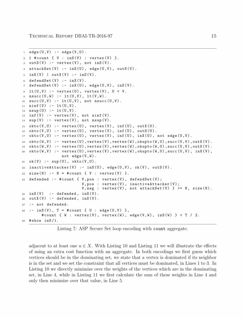
The Secure Set problem asks for a set of vertices S in a graph G such that for each subsetX ⊆ S, |N [X] ∩ S| ≥ |N [X] \ S| holds, where N [X] is the closed neighborhood of X in G,i.e., the set X together with all vertices adjacent to some vertex in X. For this problem weused the encodings in Listing 6 to Listing 9, which have been introduced and thoroughlyexplained in [1]. The first three encodings use the concept of loops, the difference betweenthe ones in Listing 6 and Listing 7 lying in the formula we use for determining if a set issecure or not, using either a sum or a count aggregate. The encoding in Listing 8 uses bordervertices to define secure sets, besides the concept of loops. In Listing 9 we have an encodingthat uses a different approach.

In order to avoid using loops we guess a partition of the attack set into active and inactive


1 edge(U,V) :- edge(V,U).

2 1 #count { V : inS(V) : vertex(V) }.

3 outS(V) :- vertex(V), not inS(V).

4 attackSet(V) :- inS(U), edge(U,V), outS(V).

5 inX(V) | outX(V) :- inS(V).

6 defendSet(V) :- inX(V).

7 defendSet(V) :- inX(U), edge(U,V), inS(V).

8 lt(U,V) :- vertex(U), vertex(V), U < V.

9 nsucc(U,W) :- lt(U,V), lt(V,W).

10 succ(U,V) :- lt(U,V), not nsucc(U,V).

11 ninf(V) :- lt(U,V).

12 nsup(U) :- lt(U,V).

13 inf(V) :- vertex(V), not ninf(V).

14 sup(V) :- vertex(V), not nsup(V).

15 okto(V,U) :- vertex(U), vertex(V), inf(U), outX(U).

16 okto(V,U) :- vertex(U), vertex(V), inf(U), outS(U).

17 okto(V,U) :- vertex(U), vertex(V), inf(U), inX(U), not edge(U,V).

18 okto(W,V) :- vertex(U),vertex(V),vertex(W),okto(W,U),succ(U,V),outX(V).

19 okto(W,V) :- vertex(U),vertex(V),vertex(W),okto(W,U),succ(U,V),outS(V).

20 okto(W,V) :- vertex(U),vertex(V),vertex(W),okto(W,U),succ(U,V), inX(V),

not edge(V,W).

21 ok(V) :- sup(U), okto(V,U).

22 inactiveAttacker(V) :- inS(U), edge(U,V), ok(V), outS(V).

23 defended :- #sum { 1,V,pos : vertex(V), defendSet(V);

1,V,pos : vertex(V), inactiveAttacker(V);-1,V,neg : vertex(V), attackSet(V) } >= 0.

24 inX(V) :- defended , inS(V).

25 outX(V) :- defended , inS(V).

26 :- not defended.

27 :- inS(V), T = #count { U : edge(U,V) },

#count { W : vertex(V), vertex(W), edge(V,W), inS(W) } < T / 2.

28 #show inS/1.

Listing 6: ASP Secure Set loop encoding.

attackers instead of a subset X of S. Further, for performance reasons all encodings for SecureSet we use in this technical report have an extra last constraint, compared to those in [1],that throws away all answer set candidates that contain vertices in S with less neighbors inS than outside of it.

3.1.3 Minimum Weighted Dominating Set

Finally, we will present two encodings for Minimum Weighted Dominating set. The task isto compute all vertex-weight-minimal dominating sets of an undirected graph G = (V,E).A subset X of V is a dominating set of G if for each v ∈ V the vertex is part of X or v is






5 inX(V) | outX(V) :- inS(V).













18 okto(W,V) :- vertex(U),vertex(V),vertex(W),okupto(W,U),succ(U,V),outX(V).

19 okto(W,V) :- vertex(U),vertex(V),vertex(W),okupto(W,U),succ(U,V),outS(V).

20 okto(W,V) :- vertex(U),vertex(V),vertex(W),okupto(W,U),succ(U,V), inX(V),

not edge(V,W).



23 size(N) :- N = #count { V : vertex(V) }.

24 defended :- #count { V,pos : vertex(V), defendSet(V);

V,pos : vertex(V), inactiveAttacker(V);V,neg : vertex(V), not attackSet(V) } >= N, size(N).



27 :- not defended.



29 #show inS/1.

Listing 7: ASP Secure Set loop encoding with count aggregate.

adjacent to at least one u ∈ X. With Listing 10 and Listing 11 we will illustrate the effectsof using an extra cost function with an aggregate. In both encodings we first guess whichvertices should be in the dominating set, we state that a vertex is dominated if its neighboris in the set and we set the constraint that all vertices must be dominated, in Lines 1 to 3. InListing 10 we directly minimize over the weights of the vertices which are in the dominatingset, in Line 4, while in Listing 11 we first calculate the sum of these weights in Line 4 andonly then minimize over that value, in Line 5.






5 border(U) :- inS(U), outS(V), edge(U,V).

6 inX(V) | outX(V) :- border(V).

7 outX(V) :- inS(V), not border(V).













20 okto(W,V) :- vertex(U),vertex(V),vertex(W),okto(W,U),succ(U,V),outX(V).

21 okto(W,V) :- vertex(U),vertex(V),vertex(W),okto(W,U),succ(U,V),outS(V).

22 okto(W,V) :- vertex(U),vertex(V),vertex(W),okto(W,U),succ(U,V), inX(V),

not edge(V,W).







28 :- not defended.



30 #show inS/1.

Listing 8: ASP Secure Set border loop encoding.

3.2 Experiments

In order to find out the treewidths of the groundings of the encodings when applied to trafficnetwork instances, we first fed each combination of an encoding and an instance to gringo4.5.0 [19,21] and then ran DynASP 2.0 [18] five times with options -d -c1, -d -c4 and -d -c5each to determine the primal, incidence and incidence-weighted-primal treewidth, respec-tively and always took into consideration the smallest among the five resulting treewidthsprovided by DynASP. The incidence-weighted-primal treewidth is the treewidth of a modi-





4 border(U,V):- inS(U), outS(V), edge(U,V).

5 attackSet(V) :- border(U,V).

6 activeAttacker(V) | inactiveAttacker(V) :- attackSet(V).

7 inX(U) : border(U,V) :- activeAttacker(V), outS(V).

8 defended :- inactiveAttacker(U), inX(V), edge(U,V).






13 activeAttacker(V) :- defended , attackSet(V).

14 inactiveAttacker(V) :- defended , attackSet(V).

15 :- not defended.



17 #show inS/1.

Listing 9: Alternative ASP Secure Set encoding.

1 { in(X) : vertex(X) }.

2 dominated(Y) :- in(X), edge(X,Y).

3 :- vertex(X), not in(X), not dominated(X).

4 #minimize { W,X: in(X), weight(X,W) }.

Listing 10: ASP Minimum Weighted Dominating Set encoding.

fication of the incidence graph, such that the literals of all choice heads and weighted bodies(for details please see [32]) each form a clique. Weighted bodies appear in the groundingwhen using aggregate functions. The used instances represent rail traffic networks, such asmetro, tram and train networks, of cities, metropolitan areas or states, having treewidthsof 2, 3 and 4 and at most 70 vertices. The graphs were extracted from mass transit datafeedsthat are publicly available using gtfs2graphs [16] and split by transportation type, such

1 { in(X) : vertex(X) }.

2 dominated(Y) :- in(X), edge(X,Y).

3 :- vertex(X), not in(X), not dominated(X).

4 cost(C) :- C = #sum { W,X: in(X), weight(X,W) }.

5 #minimize { C : cost(C) }.

Listing 11: ASP Minimum Weighted Dominating Set encoding with aggregate.


Primal Treewidth

Tree

wid

th o

f Gro

unde

d P

rogr

am

050

100

150

# 1

● ● ● ● ● ● ● ● ● ● ● ● ● ● ● ● ● ● ● ● ● ● ● ● ● ●●

● ● ●●

● ●

● ●

●

● ●

●

●

●

●● ●

●

●●

●● ● ● ●

●●

●

●

●●

● ●

●

Listing 2Listing 3Listing 4

Incidence Treewidth

Tree

wid

th o

f Gro

unde

d P

rogr

am

050

100

150

# 1

●● ● ● ● ● ● ● ● ● ● ● ● ● ● ● ● ● ● ● ● ● ● ● ● ●

●● ● ●

●

● ●

● ●

●

● ●

●

● ● ● ● ●

●

●●

● ● ●●

●●

● ●

●

●●

●

●

●


Incidence−Weighted−Primal Treewidth

Tree

wid

th o

f Gro

unde

d P

rogr

am

050

100

150

# 1

●● ● ● ● ● ● ● ● ● ● ●

●

● ● ● ● ● ● ● ● ● ● ●● ● ●

●● ● ●

● ●

● ●

●

● ●

●

● ● ● ● ●

●

●●

●● ● ● ●

●●

●

●

●●

●

●

●


0.00 0.02 0.04 0.06 0.08 0.10

0.5

0.6

0.7

0.8

0.9

1.0

Runtime

Time (s)

Qua

ntum

of I

nsta

nces

Sol

ved


Figure 2: Treewidths of groundings of Hamiltonian Cycle encodings and quantum of in-stances per time, solved by the latter with clingo.

as tram, metro, train and combinations thereof. For Minimum Weighted dominating set weused the same instances to create three test sets. For the first we inserted for each vertex aweight of 1, for the second we inserted random weights between 1 and 10 and for the thirdrandom weights between 1 and 100. Further, to determine the running time for the encod-ings on our set of traffic networks, we used clingo 4.5.4 [23] on a machine with an AMDOpteron [email protected] GHz processor operated with Debian 8 (jessie, kernel 3.16.0-4-amd64).


Incidence Treewidth

Tree

wid

th o

f Gro

unde

d P

rogr

am

050

010

0015

0020

0025

0030

00

● ● ●

●

●●

●

●●

●

●● ●

● ●

●

●

●

●

●●

●

●

●

●

● ● ●●

●

●

●

● ●

●

●

●

●

●

●

●

●

●●

●

●

●

●

●

●

●

●

●

●

●

●

●

●

●

●

# 1

● Listing 1Listing 2

0.0 0.5 1.0 1.5 2.0

0.4

0.5

0.6

0.7

0.8

0.9

1.0

Runtime

Time (s)

Qua

ntum

of I

nsta

nces

Sol

ved

Listing 1Listing 2

Figure 3: Treewidths of groundings of Hamiltonian Cycle encodings using transitivity andquantum of instances per time, solved by the latter with clingo.

3.2.1 Hamiltonian Cycle

In Figure 2 we present the primal, incidence and incidence-weighted-primal treewidths of thegroundings of four Hamiltonian Cycle encodings, one using transitivity, one using reachabilityand one using saturation, all applied to each of the traffic networks. In each of the first threegraphs, each vertical line stands for a traffic network instance. Further, we show the relationbetween the consumed time for solving and the quantum of instances solved. What leaps tothe eye first is the fact that for all different types of graphs of the groundings, the encodingin Listing 2, that uses transitivity, is the one producing the highest treewidths. At the sametime, the latter encoding is the slowest among the four compared in Figure 2. This can beexplained by the fact that the number of pTrans/2 instantiations can be quadratic in thenumber of vertices, leading to complex grounding graphs. This is why we dissuade fromusing such constructions that lead to the formation of a transitive closure. In addition, werecommend using encodings ensuring connectivity using the reachability approach. For thelatter, materialized in the encoding in Listing 3, the structure of the grounding graphs issimpler due to the fact that instead of pTrans/2 we have reach/1 in Line 5 and the numberof the latter are is linear in the number of vertices in the graph. This is why the groundingtreewidths all remain linear or even constant in the treewidths of the original graphs. Theincidence and incidence-weighted-primal treewidths for the groundings of the encoding basedon saturation from Listing 4 also remain linear in dependence of the original treewidth of theinstances, yet the primal treewidth also correlates with the size of the instance, in numbersof vertices, which can be explained by the presence of the rule in Line 7. Nevertheless, inmatters of running time the encoding using saturation was only slightly slower than the oneusing reachability.

Looking at the charts in Figure 3 we can see that among the encodings using transitivity,


Primal Treewidth

Tree

wid

th o

f Gro

unde

d P

rogr

am

020

4060

8010

0

# 1

Listing 4Listing 5

Incidence Treewidth

Tree

wid

th o

f Gro

unde

d P

rogr

am

2040

60# 1

Listing 4Listing 5


Tree

wid

th o

f Gro

unde

d P

rogr

am

020

4060

8010

0

# 1

Listing 4Listing 5

0.00 0.02 0.04 0.06 0.08 0.10

0.75

0.80

0.85

0.90

0.95

1.00

Runtime

Time (2)

Qua

ntum

of I

nsta

nces

Sol

ved

Listing 4Listing 5

Figure 4: Treewidths of groundings of Hamiltonian Cycle encodings using saturation andquantum of instances per time, solved by the latter with clingo.

the one in Listing 2 performs better than the one in Listing 1 both in terms of treewidth andrunning time, although the difference lies solely in replacing one occurrence of pTrans/2 withp/2 in Line 4. This can be explained by the fact that the number of pTrans/2 instantiationsis quadratic in the number of vertices when the graph is connected while the number ofp/2 instantiations corresponds to the number of edges which is quadratic in the number ofvertices only in case of a clique which is rather uncommon in traffic networks.

In Figure 4 we show how the two encodings for Hamiltonian Cycle using saturation behavew.r.t. running time and treewidth. The primal treewidth is correlated with the size of theinput graph for both encodings rises dramatically with the former. However, incidence andincidence-weighted-primal treewidth grow with the size of the input graph for the encoding


Primal Treewidth

Tree

wid

th o

f Gro

unde

d P

rogr

am

050

100

150

200

250

# 1

●●

●

●

●

●

●

●

●

●

●

●

●

●

●

●

●

●

●

● ●

●

●

●

●

● ●●

●

●

●

●

● ●

●

●

●

●

●

●

●

●

●

●

●

●●

●

●

●

●

●

●

●

●

●

●

●

●

●●

Listing 6Listing 7Listing 8Listing 9

Incidence Treewidth

Tree

wid

th o

f Gro

unde

d P

rogr

am

050

100

150

200

250

# 1

●●

●

●

●

●

●

●

●

●

●

●

●

●

●

●

●

●

●

●

● ●

●

●

●

●

●●

●

●

●

●

●●

●

●

●

●

●

●

●

● ●●

●

●

●

●

●

● ●●

●

●●

●

●

●

●●●



Tree

wid

th o

f Gro

unde

d P

rogr

am

050

100

150

200

250

300

# 1

●●

●

●

●

●

●

●

●

●

●

●

●

●

●

●

●

●

●

● ●

●

●

●

●

● ●●

●

●

●

●

●●

●

●

●

●

●

●

●

●

●●

●

●

●

●

●

●

●

●

●

●

●

●

●

●

●

●

●


0 1 2 3 4 5 6 7

0.10

0.15

0.20

0.25

0.30

0.35

Runtime

Time (s)

Qua

ntum

of I

nsta

nces

Sol

ved


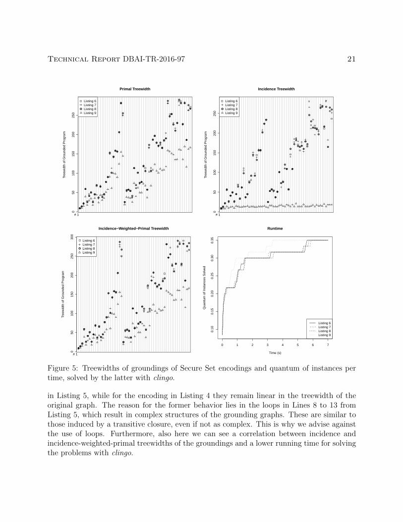
Figure 5: Treewidths of groundings of Secure Set encodings and quantum of instances pertime, solved by the latter with clingo.

in Listing 5, while for the encoding in Listing 4 they remain linear in the treewidth of theoriginal graph. The reason for the former behavior lies in the loops in Lines 8 to 13 fromListing 5, which result in complex structures of the grounding graphs. These are similar tothose induced by a transitive closure, even if not as complex. This is why we advise againstthe use of loops. Furthermore, also here we can see a correlation between incidence andincidence-weighted-primal treewidths of the groundings and a lower running time for solvingthe problems with clingo.


3.2.2 Secure Set

Another example where loops have a negative impact on running time and treewidth is oneof the Secure Set encodings, as we can see in Figure 5. The encodings that make use of aloop, namely those in Listings 6, 7 and 8, all have similar treewidths that depend on the sizesof the input instances, and are slower than the encoding in Listing 9, which avoids loops.The primal and incidence-weighted-primal treewidths for the groundings of the latter arelower than those for the groundings of the encodings with loops, yet they increase with thesize of the input graph. Similarly to the behavior of the treewidths of grounded HamiltonianCycle encodings using saturation, also here, it is the incidence treewidth that remains linearor even constant in the treewidth of the original program. Unlike in the latter case, now theincidence-weighted-primal treewidth increases due to the restriction on the count aggregate.

3.2.3 Minimum Weighted Dominating Set

Let us look at the treewidths of Minimum Weighted Dominating Set groundings and theruntime performance for the two encodings on instances which contain vertices with weightsof up to 10, in Figure 6. Primal and incidence-weighted-primal treewidths are only slightlylower for the encoding in Listing 10 than for the one in Listing 11. Incidence treewidth stayslinear or even constant in the treewidth of the input instances for the latter, while for theformer it increases with the number of vertices of the input instance. At the same time,the encoding in Listing 11 is much faster than the one in Listing 10, which leads to morecomplex incidence graphs as minimizing over a predicate that contains the sum of weightsof vertices in the dominating set instead of directly minimizing on the latter weights. Pleasenote that the treewidths are the same regardless of the values the weights of the vertices.

3.3 Impact of Rule Decomposition

As discussed earlier, when dealing with ASP programs, evaluation is usually a 2-step process.First, the program is grounded, that is, variables are replaced by all possible, valid combina-tions of symbols. Then, the solver is called on the ground program. The grounding processis exponential in the size of the rules of the program in general, but a recent rule decompo-sition tool named lpopt, presented in [6, 7] and originally based on an idea from [30], is ableto reduce this exponentiality to the treewidth of the rules. Roughly, this rule decompositiontool works by representing non-ground rules as graphs, constructing a tree decompositionof these graphs, and then splitting the rules up into multiple smaller rules based on thisdecomposition. Interestingly, it seems that, apart from decreasing the grounding size, in cer-tain instances also the treewidth of the ground program is reduced. Since the rules becomesmaller, the tool clearly reduces the primal graph treewidth of the ground program obtainedfrom the original program after applying the rule decomposition. However, as the followingexperimental tests show, interestingly, also the incidence treewidth is reduced.


Primal Treewidth

Tree

wid

th o

f Gro

unde

d P

rogr

am

010

2030

4050

6070

# 1

●●

●

●

●

●

●

●

●

●

●

●

●

●

●

●

●

●

●

●●

●

●

●

●

●●

●

●

●

●

●

●●

●

●

●

●

●

●

●

●

●●

●

●

●

●

●

●

●

●

●

●

●

●

●

●

●●

●

Listing 10Listing 11

Incidence Treewidth

Tree

wid

th o

f Gro

unde

d P

rogr

am

1020

3040

5060

70

●●

●

●

●

●

●

●

●

●

●

●

●

●

●

●

●

●

●

●●

●

●

●

●

●●

●

●

●

●

●

●●

●

●

●

●

●

●

●

●

●●

●

●

●

●

●

●

●

●

●

●

●

●

●

●

●●

# 1

●



Tree

wid

th o

f Gro

unde

d P

rogr

am

1020

3040

5060

70

●●

●

●

●

●

●

●

●

●

●

●

●

●

●

●

●

●

●

●

●●

●

●

●

●

●●

●

●

●

●

●●

●

●

●

●

●

●

●

●

●●

●

●

●

●

●

●

●

●

●

●

●

●

●

●

●●

# 1

●


0 20 40 60 80 100

0.50

0.55

0.60

0.65

0.70

0.75

0.80

Runtime

Time (s)

Qua

ntum

of I

nsta

nces

Sol

ved


Figure 6: Treewidths of groundings of Minimum Weighted Dominating Set encodings andquantum of instances per time, solved by the latter with clingo.

3.3.1 Experiment Setup

For evaluating lpopt ’s impact on ground incidence treewidth, we have considered threesources of problem instances:

1. The 200 2-QBF instances evaluated in [7], encoded in the new paradigm presentedthere, once before and once after being preprocessed by DepQBF [27]. For each in-stance, this paradigm yields a program with a long rule which makes it an archetypeapplication for lpopt.


2. 20 different voting problem encodings taken from the Democratix project5 [12] togetherwith 315 instances from the PrefLib project6.

3. Instances from the Fifth Answer Set Programming Competition 20147, providing twoencodings for most of the 25 problems: one from 2013 and one from 2014, each with 20instances. The impact of lpopt on grounding sizes and running times of these instanceshas already been investigated in [6].

Note that evaluation requires a logic program to be decomposable by lpopt at all, otherwise“common” groundings would be the same as lpopt-assisted ones. Due to not being lpopt-decomposable, the following instances could not be evaluated: “classic” 2-QBF encodingsfrom [7], secure set encodings from [1] and Steiner tree problems taken from the D-FLATproject8 [8].

For each instance, evaluation has been performed in the following manner:

1. (optional) Decompose the instance with lpopt in order to split up rules

2. Ground the instance using gringo 4.5.4 [23]

3. Run DynASP 2.0 [18] with options -d -c4 on the grounding to determine its incidencetreewidth

If, for any given instance, either the plain program or the lpopt-decomposed version ran intoa timeout or a memory overflow in any of these steps, then this instance was consideredincomparable.

For the 2-QBF instance set, evaluation was performed on an Intel Xeon E5345 2.33 GHzmachine with gringo limits set to 10 minutes and 6 GB and DynASP limits set to 15 minutesand 48 GB. The voting instances were evaluated on the same machine with limits set to 10minutes and 6 GB for both gringo and DynASP. The ASP competition instance sets wereevaluated on an AMD Opteron 6308 3.5 GHz machine with the only limit being 5 minutesfor DynASP.

3.3.2 Results

In the 2-QBF case, due to the very big rules, only few instances could have been groundedin the non-lpopt-assisted case within the time and memory limits. Additionally, DepQBF -preprocessed instances that have already been solved by the preprocessing were considereduninteresting and thus omitted from graphical representation. Therefore, as can be seen inFigure 7, out of the 400 instances (200 plain, 200 DepQBF -preprocessed), only 8 have beenconsidered comparable (four plain, the same four DepQBF -preprocessed). Nevertheless, the

5http://democratix.dbai.tuwien.ac.at/6http://www.preflib.org/data/packs/soc.zip7https://www.mat.unical.it/aspcomp2014/8http://dbai.tuwien.ac.at/research/project/dflat/system/

http://democratix.dbai.tuwien.ac.at/

http://www.preflib.org/data/packs/soc.zip

https://www.mat.unical.it/aspcomp2014/

http://dbai.tuwien.ac.at/research/project/dflat/system/


Figure 7: Incidence treewidths of groundings of comparable instances, with lpopt and withoutit (“native”). Instances are sorted by native treewidth. The left plot shows the results forthe 8 comparable 2-QBF instances in the paradigm used in [7]. The right plot shows theresults for the 6 comparable instances of the valves location problem in ASP competition’s2013 encoding.

2-QBF evaluation and Figure 7 suggest that the method of rule decomposition stronglyreduces the ground incidence treewidths of these programs.

For voting, ground incidence treewidth was found to be de facto independent of whetherlpopt was applied: 11 out of 20 problems have been found comparable (that is, contain com-parable instances), each of which only shows in exceptional cases an lpopt-induced minimalchange in ground incidence treewidth (both up and down).

The 187 comparable instances of the ASP competition show lpopt impact only in threeproblems:

The ground treewidth of the valves location problem of 2013, depicted right in Figure 7,benefits from the decomposition, although grounding size and solving time evaluation in [5]shows no significant impact. Here, lpopt is able to split up one rule without having tointroduce auxiliary domain rules.

The ground treewidth of the weighted sequence problem of 2014 quite heavily suffers fromthe decomposition, though evaluation in [5] only shows a slight increase in grounding size(about 5 %). Here, lpopt introduced an auxiliary domain rule using an intensional predicate,which causes the observed deterioration. For a discussion on auxiliary domain rules andwhy they are needed, we refer to [6]. At this point, it suffices to mention that non-groundauxiliary domain rules potentially introduce cycles, which do not manifest themselves in theprogram’s ground incidence graph if they only use extensional predicates (as then the bodyis grounded away).

The crossing minimization problem in the 2013 encoding also has its ground incidencetreewidth increased when being treated by lpopt, though evaluation in [5] depicted a ground-ing size reduction by about 50% (again, with no significant runtime changes). Also here, anauxiliary domain rule is introduced using a guessed (and therefore intensional) predicate.


3.3.3 Discussion

The question of which predicates to select for auxiliary domain rules has already been posedin [5,6]. As of the current version of lpopt, this selection is being computed by a simple greedyalgorithm that does not take into account whether predicates are extensional or intensional.The paper [6] raised awareness that the number of ground rules, and therefore the groundingsize, depends on this selection. The work [5] suggested that the selection algorithm alsorespect whether candidate predicates are intensional or extensional, and avoid intensionalones. This would best be accomplished by incorporating rule decomposition into a grounder,since grounders like gringo are already aware of which predicates are intensional and whichare extensional.

As the results show, rule decomposition is able to reduce the ground incidence treewidthof answer set programs. In a few cases, the treewidth deteriorated by rule decomposition,which may be avoided by including decomposition into the grounding process and prevent-ing intensional predicates from being selected for auxiliary domain rules. If done so, ourexperiments show no reason for rule decomposition to increase ground incidence treewidth.

4 Theoretical Investigation of Modeling Techniques

Our observations from Section 3 suggest that a problem can often be modeled in multi-ple ways that lead to quite different relationships between the “input treewidth” (i.e., thetreewidth of the input graph) and the “output treewidth” (i.e., the primal or incidencetreewidth of the grounding). In particular, some encodings are “well-behaved” in the sensethat they preserve bounded treewidth. By this we mean that the output treewidth can bebounded from above by a function that depends only on the input treewidth. Other en-codings, however, may destroy bounded treewidth in the sense that the output treewidthcannot be bounded by the input treewidth alone but depends on the input size. We wouldlike to identify which modeling techniques are responsible for this. In this section we firstgive some examples of such “ill-behaved” modeling techniques. We then characterize a classof non-ground ASP programs that excludes those techniques, and we prove that encodingsfrom this class preserve bounded treewidth.

4.1 Modeling Techniques That Destroy Bounded Treewidth

In this section, we give a small selection of modeling techniques that have to be avoided ifbounded treewidth is to be preserved. Note, however, that this is not a complete list andthat other techniques may also destroy bounded treewidth. In the following, we assume thatthe input graph is directed and given by the unary vertex predicate v and the binary edgepredicate e.

ASP grounders do not blindly instantiate the variables with all possible constants. In-stead, they try to minimize the number of produced rules by suppressing ground rules whosebody can never be satisfied by any model of the program. This property is also crucial for


the treewidth of the resulting program, since blindly instantiating each variable with everyconstant almost always leads to unbounded output treewidth.

For our investigation, we therefore assume that a ground rule is suppressed from thegrounding if it contains an extensional literal that is not a consequence of the input facts.This is the only assumption that we make on grounders in this work. For instance, thisexcludes that a grounding contains a rule p(x,y):- e(x,y) if (x, y) is no edge in the inputgraph.

As a first example, consider the rule p(X,Y):- v(X), v(Y). This destroys boundedtreewidth even for graphs without any edges: The output graph (i.e., the primal or inci-dence graph of the grounding) contains the complete graph Kn as a minor, where n is thenumber of input vertices. The problem here is that this rule allows for a too liberal instan-tiation of the variables in the sense that the edges in the output graph are not restricted byedges in the input graph.

As an attempt to remedy this, we may impose the restriction on each rule r that allvariables of r must be “chained together” by edge predicates in the positive body of r.Unfortunately this is not enough: Already a simple rule like p(X,Z):- e(X,Y), e(Y,Z) destroysbounded treewidth. To see this, consider the class of all stars, i.e., undirected graphs whereone vertex is adjacent to all other vertices, and let the class of input graphs be its directedversion, where we have the directed edges (a, b) and (b, a) instead of an undirected edge{a, b}. Clearly this class has bounded treewidth because stars are trees. However, whengiven a star with n vertices, the output graph has linear treewidth because it contains thecomplete bipartite graph Kn−1,n−1 as a minor. Instead of further restricting the syntax ofthe rules, in this work we impose a restriction on the input graphs, namely that they havebounded degree.

Even for input graphs of bounded degree, it is crucial that the atoms that connect thevariables in each rule appear in the positive body. Otherwise we could construct a programlike the following.

p(X,Y) :- v(X), v(Y), not e(X,Y).

p(X,Y) :- v(X), v(Y), e(X,Y).

Here, for any input graph having n vertices, the output graph contains Kn as a minor.Another observation is that it is important that the atoms that connect the variables of a

rule are extensional. Otherwise the following program would be allowed, which materializesthe transitive closure of the edge relation.

t(X,Y) :- e(X,Y).

t(X,Z) :- t(X,Y), e(Y,Z).

For any connected input graph, the output graph would again contain Kn as a minor. Inthe restriction that we explore in this work, we exclude this because in the second rule X isnot part of an extensional atom. An alternative approach could be to avoid the constructionof transitivity by disallowing a certain kind of cycles in a dependency graph of the program,similar to the concept of tightness in ASP. We will not pursue that approach in this work,however, and leave it for future work.


In fact, real-world grounders perform certain optimizations, which we ignore in this work,that would not lead to the treewidth being destroyed by some of our examples. For instance,if we have the rule p(X,Y):- v(X), v(Y), then Kn would not be a minor of the output graphof real-world grounders. The reason is that they may simplify every ground instantiationof this rule by removing both extensional atoms from the body because these atoms followfrom the input facts and are thus true in every model. In our conception of a grounder,such simplifications are not performed. However, this is not a huge restriction because wecould easily adapt this example to again destroy bounded treewidth even for grounders thatperform such simplifications: We could replace both occurrences of the predicate v in thebody by a new predicate w and add a rule like {w(X) : v(X)}, which guesses for each vertex xwhether w(x) is true. A grounder would not be able to simplify the resulting rule p(x,y):-

w(x), w(y) because the body atoms are not deterministic consequences of the input.

4.2 A Treewidth-Preserving Class of Non-Ground ASP

The “ill-behaved” modeling techniques from Section 4.1 destroy bounded treewidth, butthey are not necessary conditions. We still lack a positive result that indicates under whichcircumstances bounded treewidth is preserved. As we have seen, bounded treewidth is arelatively fragile property, meaning that already quite simple ASP programs destroy it.Hence we focus on preserving bounded treewidth together with bounded degree instead,which is more robust.

In this section, we present a class of ASP programs that preserves bounded treewidth forgraphs of bounded degree. In fact, we even show that bounded clique-width together withbounded degree leads to groundings of bounded treewidth because bounded clique-widthand bounded treewidth coincide on graphs of bounded degree [13, Corollary 1.53]. Beforewe define our class, we first need to formalize the notion of “chaining variables together”from Section 4.1. The idea is to restrict the structure of the output graph in a certain wayby the structure of the input graph.

Definition 2. Let r be a (non-ground) ASP rule. The join graph of r is the graph whosevertices are the variables in r and where there is an edge between two variables if thesevariables occur together in some positive body atom in r. The variables of r are connectedif they occur in a positive extensional body atom in r and the join graph of r is connected.

This allows us to define the class of programs that is of interest for this work.

Definition 3. We call a (non-ground) ASP program Π structure-restricted if, for each ruler in Π, the variables of r are connected.

We use this class to state the main theorem of this work.

Theorem 4. Let Π be a structure-restricted ASP program and G be a graph. The primaland incidence graph of the grounding of Π together with G (as a set of facts) have boundedtreewidth and bounded degree if G has bounded clique-width and bounded degree.


We prove Theorem 4 using the framework of MSO transductions. First we discuss howwe can turn a structure-restricted ASP program Π into a certain normal form to simplifythe proof. Then we state the formulas that define our transduction, which formalizes howthe incidence graph of the grounding of Π together with facts describing a graph G can beconstructed from G. Finally, we discuss why this constitutes a proof of Theorem 4.

Simplifying the ASP program. Let Π be a structure-restricted ASP program. In thefollowing, we use Π to construct a simplified program Γ together with a set of facts F suchthat, for every set of facts G that describe an input graph, Π∪G is equivalent to Γ∪F ∪G.

To obtain Γ from Π, we first eliminate constants by the following rewriting: We introducea new unary predicate Ca for each constant a. Then, for each constant a and each rule rcontaining a, we replace each occurrence of a by a new variable Xa and we add Ca(Xa) tothe positive body of r. Finally, for each such new predicate Ca, we put a fact Ca(a) into F .

We call variables that we added to replace constants constant variables and all othervariables proper variables. We denote the set of all new predicates Ca that we added to replaceconstants a by CV(Γ). Since Π is structure-restricted and thus has connected variables ineach rule, Γ has connected proper variables in each rule, but the constant variables need notbe connected. However, these will only be instantiated in a controlled way due to the factswe added to F .

Next, we eliminate propositional atoms and enforce that each rule in Γ contains at leastone proper variable: We add an atom dummy(X) to the positive body of each rule in Γ, whereX is a new proper variable and dummy is a new predicate, then replace each propositionalatom q with q(X) and put a fact dummy(a) into F , where a is an arbitrary new constant.

In the following, we consider Π (and thus Γ and F ) to be fixed and write n to denote themaximum number of distinct variables that occur in a rule of Γ.

Specifying the input graphs. Input graphs are simple, ordered and directed graphswhose maximum degree is bounded by some constant d. The input structures of our MSOformulas encode such graphs as well as the facts in F , which we obtained from Π. Hencethe domain of an input structure not only contains vertices of the input graph but alsoobjects that correspond to constants in F . The signature of input structures contains aunary “vertex” relation and binary “edge” relation, which are used for specifying the inputgraph, as well as the unary relations in CV(Γ) ∪ {dummy} for encoding F .

Even though the MSO transduction that we present in this work operates on graphsdirectly instead of their incidence structures, it not only preserves bounded clique-width butalso bounded treewidth. This is because (a) we restrict ourselves to simple input graphs ofbounded degree, (b) our transformation preserves bounded degree, and (c) it is known thatbounded clique-width and bounded treewidth coincide on simple graphs of bounded degree.

The following formula states which structures our transformation is defined for, by ex-pressing that the maximum degree is at most d and each predicate in the set CV(Γ) ∪


{dummy} has exactly one domain element in its extension.

χ ≡ ∀x¬∃y1 · · · ∃yd+1

( ∧1≤i<j≤d+1

yi 6= yj ∧d+1∧i=1

(edge(x, yi) ∨ edge(yi, x)

))∧

∧P∈CV(Γ)∪{dummy}

∃x(P (x) ∧ ¬∃y

(x 6= y ∧ P (y)

))

Auxiliary formulas. We will use the following auxiliary formulas to express that a vertexy is the i-th direct successor of a vertex x, for 1 ≤ i ≤ d:

edgei(x, y) ≡ edge(x, y) ∧ ¬∃z

(z < y ∧ edge(x, z) ∧

i−1∧j=1

¬ edgej(x, z)

)

The proper variables of each rule r must be connected in the join graph. Hence, for anypair of proper variables x, y that occur together in r, we can observe that the body of everyground instantiation of r that substitutes x and y with vertices that are “too far apart” willalways be false under any interpretation that encodes the input graph, since we cannot inferextensional atoms. Such instantiations will not be produced by a reasonable grounder. Tobe precise, two vertices are “too far apart” from another if the distance between them is atleast n: There are at most n distinct variables in a rule, so we can only make at most n− 1steps from any vertex. Since the program is fixed and d is a constant, for each vertex v thereis a constant number of vertices that we can reach from v in n steps. With this in mind, wedefine the formula reach(i1,...,ik)(x, y), for 0 ≤ k ≤ n, to express that y is reachable from xvia a sequence of vertices (x0, x1, . . . , xk) such that x0 = x, xk = y, and xj is the ij-th directsuccessor of xj−1, for 1 ≤ j ≤ k. We write ε to denote the empty tuple.

reachε(x, y) ≡ x = y

reach(i1,...,ik)(x, y) ≡ ∃z(reach(i1,...,ik−1)(x, z) ∧ edgeik(z, y)

)for 1 ≤ k ≤ n

Since the maximum degree is at most d, we can uniquely identify each path of lengthat most n by the starting vertex and a number in {0, . . . ,

∑ni=1 d

i}. We call every elementof {0, . . . ,

∑ni=1 d

i} a path number. For every path number p, we write p to denote the edgesequence of p, i.e., the sequence of direct successor indices that is uniquely identified by p.(For our purposes it does not matter which edge sequence gets which path number, but werequire that different edge sequences have different path numbers.)

There can be multiple paths from x to y. We will need to single out one of them for ourtransduction. For each path number p, we therefore define the formula fpp(x, y), which istrue iff p is the smallest path number that encodes an actual path from x to y.

fpp(x, y) ≡ reachp(x, y) ∧p−1∧q=0

¬ reachq(x, y)


We call a path number p valid from an input vertex a if there is an input vertex b suchthat fpp(x, y) evaluates to true under x 7→ a, y 7→ b.

For each path number or constant p, we define an auxiliary formula correctp(x, y) thatis true iff y is interpreted by the domain element denoted by p (where the value of x is usedas the starting vertex if p is a path number).

correctp(x, y) ≡

{fpp(x, y) if p is a path number

Cp(y) if p is a constant

Constructing the output graph. Using these auxiliary formulas, we define the remain-ing formulas of our MSO transduction.9 The class of input graphs is characterized by theformula χ from above. Our transduction formalizes how we can turn an input graph repre-sented as a set of facts G into the incidence graph of the program obtained by groundingΓ ∪ F together with G.

To make things easier to read, we do not use integers as the indices i, j of δi and θi,j, butobjects that make the intended meaning of the respective formulas clearer. For instance,for every propositional atom q, we will define a formula δq(x) that will evaluate to true forexactly one domain element that we use to interpret the free variable x; the intended purposeof the corresponding output vertex is to represent the atom q in the incidence graph of thegrounding. Using objects such as q as an index obviously does not change the nature of theapproach but can be seen as “syntactic sugar” since there is a constant number of objectsthat we use as indices in this way.

For every predicate P of (positive) arity k and for each sequence p1, . . . , pk−1 of pathnumbers or constants, we define a formula δP [p1,...,pk−1](x) that is true iff we interpret x by aninput vertex a such that each pi that is a path number is valid from a. The idea is that foreach sequence b1, . . . , bk−1 such that bi is a constant or reachable from a in at most n stepswe put a copy of a into the output graph to represent the ground atom P (a, b1, . . . , bk−1).

δP [p1,...,pk−1](x) ≡k−1∧i=1

∃y correctpi(x, y)

We proceed in a similar way with rules. In contrast to before, we only make copiesfor each possible value of the proper variables and we ignore the constant variables, sincea reasonable grounder will only instantiate these by the constants they actually stand for.For each rule r in Γ with k proper variables (k > 0) and each sequence of path numbersp1, . . . , pk−1, we define the following formula.

δr[p1,...,pk−1](x) ≡ vertex(x) ∧k−1∧i=1

∃y correctpi(x, y)

Here the conjunct vertex(x) makes sure that we only make copies of actual input vertices,but not of domain elements that only stand for constants.

9In fact our MSO transduction happens to be a first-order transduction.


We now define the formulas that specify the edges of the output graph. Let r be arule with (a positive number of) proper variables X1, . . . , Xk and (a non-negative numberof) constant variables Xk+1, . . . , Xk+m that stand for constants we denote by c1, . . . , cm,respectively, and let p1, . . . , pk−1 be a sequence of path numbers. Let P be a predicateof (positive) arity l and let AP (r) be the set of tuples (i1, . . . , il) of integers such thatP (Xi1 , . . . , Xil) occurs in r. We first define the following auxiliary formula:

compatr,P (x1, . . . , xk+m, y1, . . . , yl) ≡∨

(i1,...,il)∈AP (r)

l∧j=1

yi = xij

The intuition is that a structure satisfies compatr,P (x1, . . . , xk+m, y1, . . . , yl) iff it inter-prets the variables of r in such a way that the ground instantiation of r according to thevalues of x1, . . . , xk+m contains an atom P (a1, . . . , al) such that a1, . . . , al are exactly thevalues of y1, . . . , yl. We use this to make sure that whenever we instantiate the variables ofr in such a way that the resulting ground rule r′ contains P (a1, . . . , al), the incidence graphof the output program contains an edge between P (a1, . . . , al) and r′. For each sequence ofpath numbers or constants q1, . . . , ql−1, we therefore define the following formula:

θr[p1,...,pk−1],P [q1,...,ql−1](x, y) ≡ ∃x1 · · · ∃xk+m∃y1 · · · ∃yl(x = x1 ∧ y = y1

∧ correctp1(x, x2) ∧ · · · ∧ correctpk−1(x, xk)

∧ Cc1(xk+1) ∧ · · · ∧ Ccm(xk+m)

∧ correctq1(y, y2) ∧ · · · ∧ correctql−1(y, yl)

∧ compatr,P (x1, . . . , xk+m, y1, . . . , yl))

Obtaining the actual incidence graph from the result. This MSO transductiondefines a graph that differs in the following ways from the incidence graph of the grounding ofΠ together the facts describing the input graph: First, the output graph may contain severalisolated vertices that are not in the incidence graph of the grounding. For instance, theformula δedge[p](x), where p is some path number, evaluates to true under every interpretationof x even if this vertex has no neighbors at all. This causes that the output graph may containa vertex that corresponds to an atom edge(a, b) while there is no such edge in the input graph.However, this does not matter because we can just delete such vertices without destroyingbounded treewidth or clique-width.10

The second difference between the output graph and the incidence graph of the groundingis that our MSO transduction does not take care of the facts encoding the input graph,whereas for every such fact the grounding contains a rule vertex that is connected to therespective atom vertex. It is easy to see that adding the missing rule vertices and connectingthem with the respective atom vertices increases the treewidth or clique-width by at most 1.

10The class of graphs of bounded treewidth and the class of graphs of bounded clique-width are bothhereditary (i.e., closed under taking subgraphs).


Finally, the output graph contains atom vertices involving the predicates from CV(Γ) ∪{dummy}, which are not present in the incidence graph of the grounding. Again, we canjust delete these vertices and their incident edges without increasing the treewidth or clique-width.

Discussion. Recall that Π is fixed, d is bounded and the grounder does not instantiate twovariables in a rule with vertices whose distance from each other is more than n − 1. Hencethe number of produced instantiations of a rule r depends only on n and d. This impliesthat the incidence graph of the grounding also has bounded degree. As we have just seen, wecan easily obtain this graph from the output graph of the transduction without significantlyincreasing the clique-width. Furthermore, as we have already mentioned, our transductionpreserves bounded clique-width, and bounded clique-width coincides with bounded treewidthon graphs of bounded degree. It follows that grounding Π together with a set of factsdescribing an input graph of degree d leads to a program whose incidence treewidth dependsonly on d and the clique-width of the input graph. To prove Theorem 4 it remains to showthat also the primal graph has both bounded degree and bounded treewidth. The factthat the incidence graph has bounded degree clearly implies that the primal graph also hasbounded degree. It also implies that the primal graph has bounded treewidth because we canturn a tree decomposition of the incidence graph into one of the primal graph by replacingthe rule vertices in the bags with all adjacent atom vertices, which increases the treewidthonly by a constant.

5 Conclusion

In this work we investigated how the treewidth of grounded ASP programs is affected bydifferent modeling constructs in the non-ground program. We first performed experimentswith several problems and, for each problem, various modeling alternatives. As expected,certain language constructs lead to a significant increase in the treewidth of the grounding,when compared to the treewidth of the input graph. Interestingly, we observed that lowtreewidth of the grounding often correlates with low running time of state-of-the-art ASPsolvers. We then showed that splitting non-ground rules up using a recently proposed ruledecomposition technique may reduce not only the size of the groundings but also theirtreewidth.

Next, we turned to a theoretical analysis. As our experiments showed, different non-ground modeling variants lead to groundings of quite different treewidths and subsequentsolver running times. It is therefore interesting which features of non-ground ASP encodingsguarantee that the treewidth of the groundings is not significantly higher than the treewidthof the input. To clarify this, we introduced a syntactically restricted class of non-ground ASPcalled structure-restricted programs, and we showed that the treewidth of the grounding ofa structure-restricted program together with some input depends only on the degree andtreewidth (in fact even clique-width) of the input but not on its size.


Further research on the effect of the treewidth of a ground program on ASP solver runningtime is still needed to obtain a clear picture. Besides more experiments in this direction,a theoretical analysis of the solving process of CDCL-based solvers should be performed.Our experiments suggest that CDCL-based solving often implicitly takes advantage of lowtreewidth of the program. Another subject of future work is the incorporation of rule de-composition into ASP grounders. This allows us to avoid those auxiliary domain rules whichincrease the treewidth. Finally, we plan to study restrictions on non-ground programs otherthan structure-restrictedness to find other program classes that preserve bounded treewidthas well but may be employed in different situations.

References

[1] Michael Abseher, Bernhard Bliem, Gunther Charwat, Frederico Dusberger, and StefanWoltran. Computing secure sets in graphs using answer set programming. Journal ofLogic and Computation, 2015.

[2] Mario Alviano, Carmine Dodaro, Wolfgang Faber, Nicola Leone, and Francesco Ricca.WASP: A native ASP solver based on constraint learning. In Proc. LPNMR, pages54–66, 2013.

[3] Mario Alviano, Wolfgang Faber, Nicola Leone, Simona Perri, Gerald Pfeifer, and GiorgioTerracina. The disjunctive datalog system DLV. In Datalog Reloaded. Revised SelectedPapers, pages 282–301, 2010.

[4] Stefan Arnborg, Derek G. Corneil, and Andrzej Proskurowski. Complexity of findingembeddings in a k-tree. SIAM J. Algeb. Discr. Meth., 8(2):277–284, 1987.

[5] Manuel Bichler. Optimizing non-ground answer set programs via rule decomposition.BSc Thesis, TU Wien. http://dbai.tuwien.ac.at/proj/lpopt, November 2015.

[6] Manuel Bichler, Michael Morak, and Stefan Woltran. lpopt: A rule optimization toolfor answer set programming. In Proc. LOPSTR 2016. To appear. See also CoRRabs/1608.05675, 2016.

[7] Manuel Bichler, Michael Morak, and Stefan Woltran. The power of non-ground rules inanswer set programming. In Proc. ICLP. To appear. See also CoRR abs/1608.01856,2016.

[8] Bernhard Bliem, Michael Morak, and Stefan Woltran. D-FLAT: declarative problemsolving using tree decompositions and answer-set programming. TPLP, 12(4-5):445–464,2012.

[9] Hans L. Bodlaender. A linear-time algorithm for finding tree-decompositions of smalltreewidth. SIAM J. Comput., 25(6):1305–1317, 1996.

http://dbai.tuwien.ac.at/proj/lpopt


[10] Gerhard Brewka, Thomas Eiter, and Miroslaw Truszczynski. Answer set programmingat a glance. Commun. ACM, 54(12):92–103, 2011.

[11] Francesco Calimeri, Wolfgang Faber, Martin Gebser, Giomvambattista Ianni, RolandKaminski, Thomas Krennwallner, Nicola Leone, Francesco Ricca, and Torsten Schaub.ASP-Core-2 Input Language Format v2.03c, 2015. Accessed: 2016-06-27.

[12] Gunther Charwat and Andreas Pfandler. Democratix: A declarative approach to winnerdetermination. In Proc. ADT 2015, volume 9346 of LNCS, pages 253–269. Springer,2015.

[13] Bruno Courcelle and Joost Engelfriet. Graph Structure and Monadic Second-Order Logic- A Language-Theoretic Approach, volume 138 of Encyclopedia of mathematics and itsapplications. Cambridge University Press, 2012.

[14] Evgeny Dantsin, Thomas Eiter, Georg Gottlob, and Andrei Voronkov. Complexity andexpressive power of logic programming. ACM Comput. Surv., 33(3):374–425, 2001.

[15] Islam Elkabani, Enrico Pontelli, and Tran Cao Son. SmodelsA - A system for computinganswer sets of logic programs with aggregates. In Proc. LPNMR, pages 427–431, 2005.

[16] Johannes K. Fichte. daajoe/gtfs2graphs – a GTFS transit feed to graph format con-verter. https://github.com/daajoe/gtfs2graphs, 2016.

[17] Johannes K. Fichte, Markus Hecher, Michael Morak, and Stefan Woltran. Answer setsolving using tree decompositions and dynamic programming — the dynASP2 system—. Technical Report DBAI-TR-2016-101, DBAI, Fakultat fur Informatik an der Tech-nischen Universitat Wien, 2016.

[18] Johannes Klaus Fichte, Markus Hecher, Michael Morak, and Stefan Woltran. Countinganswer sets via dynamic programming. In Trends and Applications of Answer SetProgramming (KI 2016), 2016.

[19] Martin Gebser, Roland Kaminski, Benjamin Kaufmann, Marius Lindauer, Max Os-trowski, Javier Romero, Torsten Schaub, and Sven Thiele. Potassco User Guide2.0. Available at https://sourceforge.net/projects/potassco/files/guide/2.0/guide-2.0.pdf, 2015.

[20] Martin Gebser, Roland Kaminski, Benjamin Kaufmann, and Torsten Schaub. AnswerSet Solving in Practice. Synthesis Lectures on Artificial Intelligence and Machine Learn-ing. Morgan & Claypool Publishers, 2012.

[21] Martin Gebser, Roland Kaminski, Benjamin Kaufmann, and Torsten Schaub. AnswerSet Solving in Practice. Synthesis Lectures on Artificial Intelligence and Machine Learn-ing. Morgan & Claypool Publishers, 2012.

https://github.com/daajoe/gtfs2graphs

https://sourceforge.net/projects/potassco/files/guide/2.0/guide-2.0.pdf

https://sourceforge.net/projects/potassco/files/guide/2.0/guide-2.0.pdf


[22] Martin Gebser, Roland Kaminski, and Torsten Schaub. Grounding recursive aggregates:Preliminary report. CoRR, abs/1603.03884, 2016.

[23] Martin Gebser, Benjamin Kaufmann, Roland Kaminski, Max Ostrowski, TorstenSchaub, and Marius Thomas Schneider. Potassco: The Potsdam Answer Set SolvingCollection. AI Commun., 24(2):107–124, 2011.

[24] Martin Gebser, Benjamin Kaufmann, and Torsten Schaub. Conflict-driven answer setsolving: From theory to practice. Artif. Intell., 187:52–89, 2012.

[25] Michael Gelfond and Vladimir Lifschitz. The stable model semantics for logic program-ming. In Proc. ICLP/SLP, pages 1070–1080, 1988.

[26] Michael Jakl, Reinhard Pichler, and Stefan Woltran. Answer-set programming withbounded treewidth. In Proc. IJCAI’09, 2009.

[27] Florian Lonsing and Uwe Egly. Depqbf: An incremental QBF solver based on clausegroups. CoRR, abs/1502.02484, 2015.

[28] Victor W. Marek and Miros law Truszczynski. Stable Models and an Alternative LogicProgramming Paradigm. In The Logic Programming Paradigm – A 25-Year Perspective,pages 375–398. Springer, 1999.

[29] Michael Morak, Reinhard Pichler, Stefan Rummele, and Stefan Woltran. A dynamic-programming based ASP-solver. In Proc. JELIA’10, pages 369–372, 2010.

[30] Michael Morak and Stefan Woltran. Preprocessing of complex non-ground rules inanswer set programming. In Proc. ICLP, pages 247–258, 2012.

[31] Reinhard Pichler, Stefan Rummele, Stefan Szeider, and Stefan Woltran. Tractableanswer-set programming with weight constraints: bounded treewidth is not enough.Theory and Practice of Logic Programming, TPLP, 14:141–164, 3 2014.

[32] Tommi Syrjanen. Lparse 1.0 user’s manual. http://www.tcs.hut.fi/smodels/

lparse.ps.gz, 2000.

http://www.tcs.hut.fi/smodels/lparse.ps.gz

http://www.tcs.hut.fi/smodels/lparse.ps.gz

technical r eport treewidth-preserving modeling in asp

Documents