techniques for increasing the capacity of wireless broadband
TRANSCRIPT
Real Wireless Ltd
PO Box 2218
Pulborough t +44 207 117 8514
West Sussex f +44 808 280 0142
RH20 4XB e [email protected]
United Kingdom www.realwireless.biz
Techniques for increasing the
capacity of wireless broadband
networks: UK, 2012-2030
Annexes A1 - A6 Produced by Real Wireless on behalf of Ofcom
Issued to: Ofcom
Issue date: March 2012
Version: 1.15

Techniques for increasing the capacity of wireless broadband networks: UK, 2012-2030 Issue date: March 2012
Version: 1.15
Version Control
Item Description
Source Real Wireless
Client Ofcom
Report title Techniques for increasing the capacity of wireless broadband networks:
UK, 2012-2030
Sub title Annexes A1 - A6 Produced by Real Wireless on
behalf of Ofcom
Issue date March 2012
Document number
Document status
Comments
Version Date Comment
1.15 26/03/2012 Issued to Ofcom for publication

Copyright ©2012 Real Wireless Limited. All rights reserved.
Registered in England & Wales No. 6016945
About Real Wireless
Real Wireless is a leading independent wireless consultancy, based in the U.K. and
working internationally for enterprises, vendors, operators and regulators –
indeed any organization which is serious about getting the best from wireless to
the benefit of their business.
We seek to demystify wireless and help our customers get the best from it, by
understanding their business needs and using our deep knowledge of wireless to
create an effective wireless strategy, implementation plan and management
process.
We are experts in radio propagation, international spectrum regulation, wireless
infrastructures, and much more besides. We have experience working at senior
levels in vendors, operators, regulators and academia.
We have specific experience in LTE, UMTS, HSPA, Wi-Fi, WiMAX, DAB, DTT, GSM,
TETRA – and many more.
For details contact us at: [email protected]
Tap into our news and views at: realwireless.wordpress.com
Stay in touch via our tweets at twitter.com/real_wireless

Techniques for increasing the capacity of wireless broadband networks: UK, 2012-2030 Issue date: March 2012
Version: 1.15
Techniques for increasing the capacity of wireless broadband networks: UK, 2012-2030 Issue date: March 2012
Version: 1.15
Contents
A1. Site Costs ............................................................................................... 1
1.1. Introduction and overall approach ................................................................ 1
1.2. Framework and general cost modelling assumptions .................................. 1
1.3. Costs of capacity enhancing techniques ....................................................... 4
1.4. High level assessment of benefits and affordability ................................... 17
A2. Technology Considerations and Spectral Efficiency ............................... 20
2.1. Overview of Technology Characterisation by Spectral Efficiency ............... 20
2.2. Capacity Enhancing Techniques .................................................................. 20
2.3. Overview of numerical model for spectral efficiency ................................. 41
2.4. Technology Evolution from 2012-2030 ....................................................... 42
2.5. Impact of Traffic Mix and Network Utilisation ............................................ 45
2.6. Technology Evolution Scenarios Low, Mid, High:........................................ 46
2.7. Cell Spectral Efficiency Per Generation, Per Antenna Configuration .......... 47
2.8. Sectorisation Gains ...................................................................................... 51
2.9. Adjustments for Outdoor Small Cells .......................................................... 52
2.10. Site Spectral Efficiency ................................................................................. 54
2.11. Environmental Scaling for Geotypes, Carrier Frequency and Indoor Users 56
2.12. Indoor Small cells (Femtocells) .................................................................... 59
A3. Spectrum scenarios .............................................................................. 61
3.1. Introduction ................................................................................................. 61
3.2. Spectrum as a source of supply for mobile capacity ................................... 62
3.3. Quantity and timing assumptions for frequency bands .............................. 62
3.4. Spectrum scenarios ..................................................................................... 73
3.5. Modelling spectrum bands as a choice for supply ...................................... 80
A4. Site Ranges .......................................................................................... 81
4.1 Requirements .............................................................................................. 82
4.2 Modelling methodology .............................................................................. 82
4.3 Site Ranges ................................................................................................... 97
4.4 Technology Considerations ....................................................................... 101
A5. Demand assessment ...........................................................................105
5.1 Introduction ............................................................................................... 105
5.2 General approach ...................................................................................... 106
5.3 Demand methodology and detailed assumptions .................................... 111
A6. Technical model description ................................................................152
6.1 Introduction ............................................................................................... 152
6.2 Brief description ........................................................................................ 152

Techniques for increasing the capacity of wireless broadband networks: UK, 2012-2030 Issue date: March 2012
Version: 1.15
6.3 Overview of the model between 2012 and 2030 ...................................... 154
6.4 Flowchart ................................................................................................... 155
6.5 Model calibration in year 2012 ................................................................. 157
6.6 Pre-processing of data ............................................................................... 157
6.7 New sites and site upgrades ...................................................................... 162
6.8 Modelling of spectrum .............................................................................. 166
Techniques for increasing the capacity of wireless broadband networks: UK, 2012-2030 Issue date: March 2012
Version: 1.15 1
A1. Site Costs
1.1. Introduction and overall approach
This annex sets out the approach, assumptions and sources of data we use in our cost
model to estimate the costs that feed into our evaluation of the capacity enhancing
techniques studied in this project. It covers both our approach to calculating the cost inputs
used by the technical or study area models and the assumptions we use in our overall cost
benefit assessment.
First we set out the overall framework for the cost modelling, explaining the type of costs
we modelled. Then, we explain how we derived the costs for each of the capacity
enhancing techniques.
1.2. Framework and general cost modelling assumptions
1.2.1. Outline of the costs estimated
We look at network costs only and do not cover retail costs. This is because retail costs are
unlikely to vary significantly with the choices for increasing network capacity that are the
main focus of this study.
The costs we estimate comprise:
• Annual operating costs
• Capital expenditure for new equipment
• Capital expenditure for replacement investment.
We estimate current costs1 and project forward in subsequent years by applying annual
cost trends for broad equipment categories. We set out our assumptions below when we
discuss the specific capacity enhancing techniques.
For replacement investment, we model a replacement cycle – for example, a unit of
equipment deployed in year Y, will reach the end of its economic lifetime (and therefore is
likely to need to be replaced) in each year Y + L, Y + 2L, … until the end of the model period,
where L is the economic lifetime of the equipment. Each replacement will incur a cost
which will be the capital expenditure cost of a new unit of equipment in the year of
replacement.
1.2.2. Modelling timeframe
Our modelling runs over the period 2012-2030. As a result, the model may not fully capture
the cost impact of capacity enhancing techniques that are introduced towards the end of
this period. This is because capital expenditure costs are incurred up front and the lifetime
of some elements of expenditure may be long, e.g. 30 years for some civil works.
1 Most of the starting cost data are estimated for 2011 and then converted to 2012, the start of the model
period, by applying a cost trend, some costs are estimated for 2012.
Techniques for increasing the capacity of wireless broadband networks: UK, 2012-2030 Issue date: March 2012
Version: 1.15 2
Therefore, in terms of the cost modelling, we “extend” the cost model for an additional 10
years to counter this bias against techniques introduced late in the model period. This
means that we keep demand constant beyond 2030 so no completely new equipment is
installed, and we measure the operating costs plus the costs of any replacement
investment for existing equipment in that period.
1.2.3. Equipment costs are modelled explicitly, software upgrades implicitly
Many of the capacity enhancing techniques we study require changes in the network and
hence additional equipment and potentially site related build works. Some techniques are
explicitly modelled as operator choices, hence we explicitly estimate costs for the following:
• Macrocell densification
• Increased sectorisation (from 3 to 6 sectors per cell)
• Deployment of higher order MIMO (from 2 transmitters (Tx) to 4Tx and from 4Tx
to 8Tx)
• Outdoor small cell deployment
We have assessed a number of other capacity enhancing techniques (listed below) which,
unlike those mentioned above, largely require upgrades to software rather than additional
equipment.
• LTE Advanced
• Carrier Aggregation
• Co-ordinated Multipoint (CoMP)
• A range of future, as yet unspecified, technologies as notionally standardised in
3GPP Releases 12 to 20, for which we model increases in spectral efficiency.
We model these techniques “implicitly”– i.e. we assume that they will be introduced
automatically and do not model them as an operator choice in the technical model. So, we
specify technology evolution scenarios which detail when these techniques are introduced
and how spectral efficiency increases as a result. We assume that these technologies
diffuse into the network as equipment is replaced and the costs are included within
equipment costs as they evolve over time.
We specify three technology evolution scenarios with varying rates of new technology
deployment, but we assume that costs trends are the same in each scenario. Hence in the
faster innovation scenarios can be read as representing a scenario where operators (and
consumers) get greater functionality for the same expenditure. There is a number of factors
that may affect how technological progress impacts on the unit costs of equipment and it is
uncertain what the overall effect might be. For example, higher research expenditure (and
higher equipment costs) could lead to faster innovation, but not necessarily so.
1.2.4. Cost inputs for the technical model
The main capacity enhancing techniques that we explicitly model comprise a number of
macrocell related costs, including upgrades to macrocell technology, the deployment of
outdoor small cells and the deployment of additional spectrum bands.
For macrocells and outdoor small cells, the input for the technical model we estimate is the
total cost per site. We identify the type and number of equipment components necessary

Techniques for increasing the capacity of wireless broadband networks: UK, 2012-2030 Issue date: March 2012
Version: 1.15 3
to implement that technique at each site. When we discuss the individual techniques
below, we set out the breakdown of our total cost estimates.
The total cost per site feeds into the technical model, which calculates the number of new
sites and/or upgrades to existing sites required to implement a particular technique. This
enables the technical model to calculate the optimal technology to deploy in each
modelling period, i.e. the lowest cost way of meeting capacity demand.
There are two exceptions to this:
• First, indoor smaller cells (femtocells, picocells, Wi-Fi access points) are modelled
through their impact on demand – i.e. demand is off-loaded from the public
mobile network and the demand needed to be met by macrocells and outdoor
small cells is correspondingly reduced. However, there is still a cost to deploying
indoor small cells, hence we calculate this separately from the cost of the public
network.
• Second, spectrum related costs are treated differently. We input the cost of
upgrading existing macrocell sites to carry new spectrum bands to the technical
model, however we do not input the cost of acquiring new spectrum. Hence, we
add back in the spectrum costs once we have run the technical model in order to
assess whether adding a new spectrum band would be cost efficient.
We treat spectrum costs in this way because operators base their decisions to buy
spectrum over a long time period, say 15 to 20 years. This does not fit well with the much
shorter decision period, 12 months, which we use in the technical model.
1.2.5. We estimate the costs to society
Our default position is to assess costs to society. This means that we use a social rather
than an operator discount rate when calculating the present value of costs (and benefits) in
our scenarios. Further, we include any costs that consumers may incur from self-provision
of equipment as well as those operators incur. This fits in with a regulatory perspective
which is interested in the costs (and benefits) to society of decisions that could impact on
wireless broadband capacity.
However, we also recognise that operator decisions on equipment and technology
deployment do not take into account the wider costs to society. So, we carry out limited
sensitivity checking by using a commercial rather than a social discount rate.
In theory, the treatment of indoor small cells and spectrum could be different. However, for
femtocells, we assume that operators will take into account the cost of the femtocells or
Wi-Fi access points in their decisions – we see today operators who supply femtocells to the
user who pays for the femtocell directly, or indirectly through increased monthly charges.
Further, we assume that the extent to which users will need to upgrade their fixed
broadband connection as a result of deploying a femtocell, is likely to be limited. So, a
difference does not arise between the operator view and the base assumptions for the
societal view.
On spectrum costs, we have taken a relatively simple approach to estimating the cost of
spectrum –benchmarking on relevant auction prices. We consider that this is a reasonable
estimate for the value of the spectrum both to society and to an operator. We believe this
Techniques for increasing the capacity of wireless broadband networks: UK, 2012-2030 Issue date: March 2012
Version: 1.15 4
apparently simple approach is appropriate given that estimating the value of spectrum is
not the main focus of this study.
1.3. Costs of capacity enhancing techniques
This section sets out our modelling of the costs of each capacity enhancing technique that
we explicitly model, detailing our approach and sources, and summarising our estimates.
1.3.1. Techniques relating to macrocells
This section discusses macrocell densification, higher order MIMO and increased macrocell
sectorisation. We have estimated the costs as far as possible on a common basis, since the
type of equipment upgrades, if not the number of units required, will be similar.
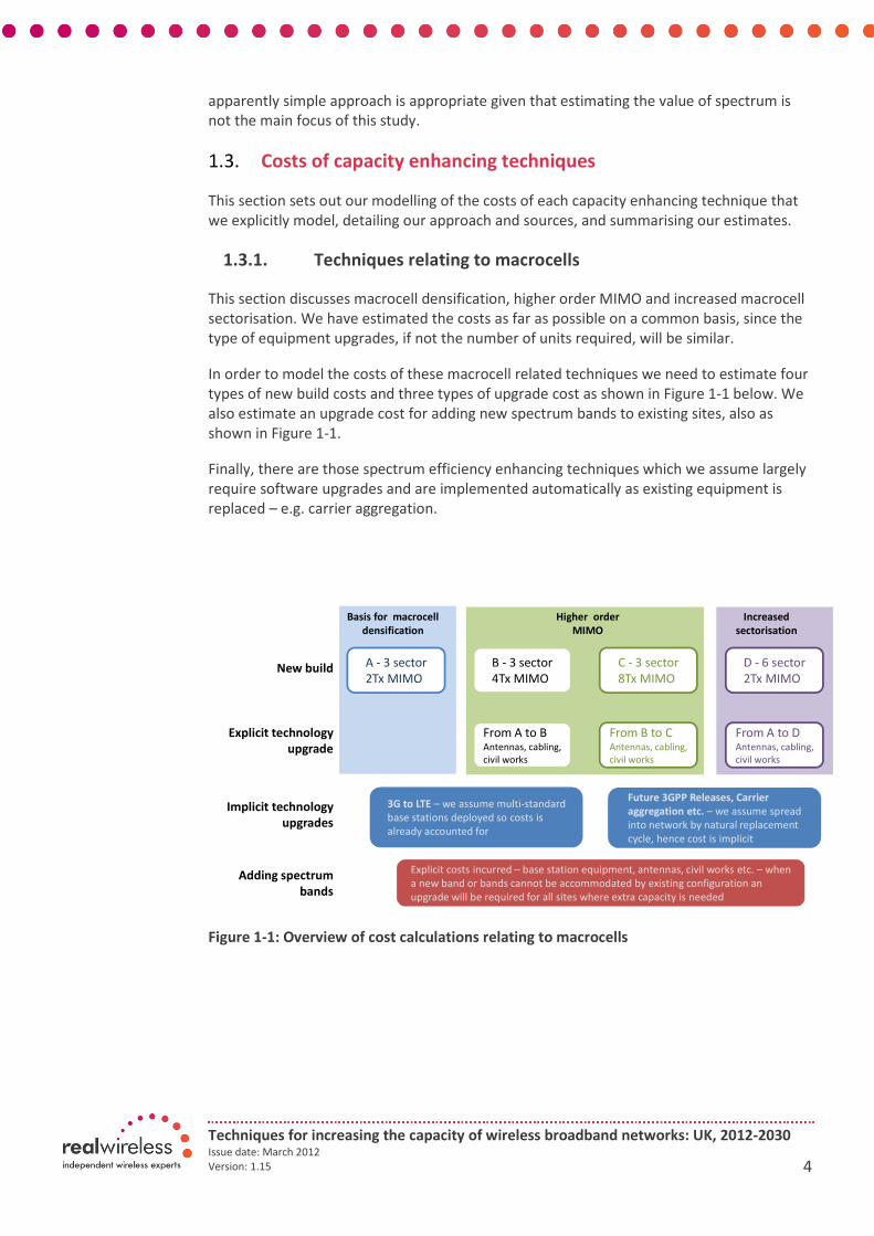
In order to model the costs of these macrocell related techniques we need to estimate four
types of new build costs and three types of upgrade cost as shown in Figure 1-1 below. We
also estimate an upgrade cost for adding new spectrum bands to existing sites, also as
shown in Figure 1-1.
Finally, there are those spectrum efficiency enhancing techniques which we assume largely
require software upgrades and are implemented automatically as existing equipment is
replaced – e.g. carrier aggregation.
Figure 1-1: Overview of cost calculations relating to macrocells
New build
Explicit technology
upgrade
Adding spectrum
bands
Implicit technology
upgrades
A - 3 sector
2Tx MIMO
Basis for macrocell
densification
B - 3 sector
4Tx MIMO
C - 3 sector
8Tx MIMO
D - 6 sector
2Tx MIMO
From A to BAntennas, cabling,
civil works
From B to CAntennas, cabling,
civil works
From A to DAntennas, cabling,
civil works
3G to LTE – we assume multi-standard
base stations deployed so costs is
already accounted for
Future 3GPP Releases, Carrier
aggregation etc. – we assume spread
into network by natural replacement
cycle, hence cost is implicit
Explicit costs incurred – base station equipment, antennas, civil works etc. – when
a new band or bands cannot be accommodated by existing configuration an
upgrade will be required for all sites where extra capacity is needed
Higher order
MIMO
Increased
sectorisation

Techniques for increasing the capacity of wireless broadband networks: UK, 2012-2030 Issue date: March 2012
Version: 1.15 5
1.3.2. Macrocell densification
We model rising unit macrocell costs with site density
The cost of deploying macrocells typically rises as the density of sites in an area increases –
for example, it may be harder to find suitable new sites because more easily accessible
(hence lower cost) sites may be acquired and built first. Also, getting planning approval may
become more difficult over time, particularly in sensitive areas in both cities and the
countryside.
We model a linear relationship between site cost and density (sites per km2). We estimate
low and high unit costs for macrocells based on our practical experience in macrocell
deployment and relate them to site density as shown in Figure 1-2 below. We assume that
the low cost estimate relates to a site density of zero for simplicity and that the high cost
estimate relates to a site density of 10 sites per km2. We derived this site density from
examining actual site densities in areas such as London where operators already face
problems in deploying more macrocell sites to cope with current congestion on existing
sites and we discussed this assumption with industry sources.
Figure 1-2: Illustration of modelling of the relationship of site costs and density
Figure 1-2 also shows a “hard limit” or maximum density of macrocells that can be
effectively deployed before radio interference becomes a significant challenge. We
assumed that this is effectively the same as the intercept on the x-axis for the high-density
cost.
Average local macro site density (sites/km2)
Co
st
Low dens High dens
Low
de
ns
cost
Hig
h d
en
s co
st
Hard limit: radio problems

Techniques for increasing the capacity of wireless broadband networks: UK, 2012-2030 Issue date: March 2012
Version: 1.15 6
Costs vary by geotype
We used our practical experience of macrocell deployment and discussion with vendors &
industry to derive representative cost estimates for three types of macrocell installation:
greenfield, rooftop and street furniture2. The cost estimates relate to a tri-sector macrocell
with a MIMO technology site configuration of 2 downlink transmit antennas (2Tx MIMO).
However, the cost efficient deployment model works at the level of study areas. Although
these areas comprise several geotypes, they can each be linked to one principal geotype –
urban, sub-urban or rural – for the purpose of cost modelling. We produce cost estimates
per geotype by taking a weighted average of the greenfield, rooftop and street furniture
costs according to the proportion of each site installation type by geotype. We estimate the
distribution of site installation types across geotypes from our practical experience of
macrocell network deployments, and the distribution is shown below in Table 1.
Urban Sub-urban Rural
Greenfield 0% 30% 80%
Rooftop 95% 60% 10%
Street
furniture
5% 10% 10%
Table 1: Assumed distribution of site installation type by geotype
The cost data
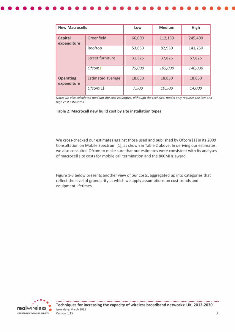
Table 2 below presents a summarised view of our macrocell cost data on operating and
capital expenditure.
For capital expenditure, we specified some 25 separate cost items such as towers, site
electrical installations, backhaul and antenna rigging for our site installation types. The
more site specific costs, such as site acquisition and design, varied by installation type
whereas others, such as antenna costs, did not. Similarly, we broke operating expenses
down into 5 constituent classes: rent; backhaul; rates; utilities costs and maintenance.
Although operating costs do vary with each specific installation, we do not believe the
variation by site installation type is consistent and significant enough that it would add
value to model it.
2 This is a macrocell as opposed to a smaller cell and we have evidence that some operators have deployed
these types of macrocell in urban locations
Techniques for increasing the capacity of wireless broadband networks: UK, 2012-2030 Issue date: March 2012
Version: 1.15 7
New Macrocells Low Medium High
Capital
expenditure
Greenfield 66,000 112,150 245,400
Rooftop 53,850 82,950 141,250
Street furniture 31,325 37,825 57,825
Ofcom1 75,000 105,000 140,000
Operating
expenditure
Estimated average 18,850 18,850 18,850
Ofcom[1] 7,500 10,500 14,000
Note: we also calculated medium site cost estimates, although the technical model only requires the low and
high cost estimates
Table 2: Macrocell new build cost by site installation types
We cross-checked our estimates against those used and published by Ofcom [1] in its 2009
Consultation on Mobile Spectrum [1], as shown in Table 2 above. In deriving our estimates,
we also consulted Ofcom to make sure that our estimates were consistent with its analyses
of macrocell site costs for mobile call termination and the 800MHz award.
Figure 1-3 below presents another view of our costs, aggregated up into categories that
reflect the level of granularity at which we apply assumptions on cost trends and
equipment lifetimes.

Techniques for increasing the capacity of wireless broadband networks: UK, 2012-2030 Issue date: March 2012
Version: 1.15 8
Figure 1-3: Breakdown of macrocell costs by broad equipment categories
We estimate current costs, i.e. for 2011, and project them forward for the period of the
model run by applying a set of cost trends to the broad equipment categories shown above.
We use the same assumptions used by Ofcom [1] in its Mobile Spectrum Liberalisation
work. Backhaul was not specified separately, so we use our own industry sources to provide
this assumption. Our assumptions on the evolution of costs are:
• Site civil works: +2.5% per annum
• Towers: +2.5% per annum
• Antennas: –7.5% per annum
• Other site equipment: –7.5% per annum
• Backhaul: –2% per annum.
1.3.3. Macrocell densification – modelling of the number of
networks
The technical model assumes that there is one network across all study areas service all
demand in order to manage modelling complexity. However, in reality there are several
mobile networks. When we amalgamate our study area results to the UK as a whole, we
want to measure the cost on a more realistic basis.
We assume that, over the course of the model, mobile broadband will be delivered over
two shared networks with traffic equally split between them. There are currently two pairs
of mobile network infrastructure providers each with network sharing agreements – MBNL
(EE-H3G) and Cornerstone (O2-Vodafone) – although not all sites are shared and each
mobile operator can elect to have a site built just to serve their needs. Further, there is a
clear trend in many countries towards greater network sharing. Hence, we believe that it is
reasonable to apply this assumption to the period we are modelling.
All Equipment
43%
Backhaul - 11%
Other
site equipment
12%
Antennas - 6%
Towers - 17%
Site civil works
& acquisition
55%
Site civil works
& acquisition
57%
£0
£10,000
£20,000
£30,000
£40,000
£50,000
£60,000
£70,000
£80,000
£90,000
£100,000
£110,000
Greenfield: medium (2011) Ofcom (2009)
Site civil works & acquisition
Towers
Antennas
Other site equipment
Backhaul
All Equipment
Techniques for increasing the capacity of wireless broadband networks: UK, 2012-2030 Issue date: March 2012
Version: 1.15 9
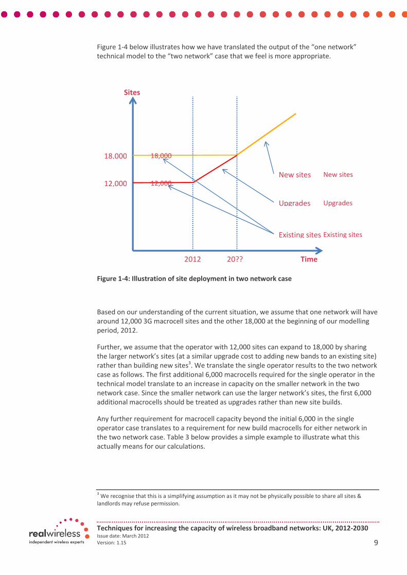
Figure 1-4 below illustrates how we have translated the output of the “one network”
technical model to the “two network” case that we feel is more appropriate.
Figure 1-4: Illustration of site deployment in two network case
Based on our understanding of the current situation, we assume that one network will have
around 12,000 3G macrocell sites and the other 18,000 at the beginning of our modelling
period, 2012.
Further, we assume that the operator with 12,000 sites can expand to 18,000 by sharing
the larger network’s sites (at a similar upgrade cost to adding new bands to an existing site)
rather than building new sites3. We translate the single operator results to the two network
case as follows. The first additional 6,000 macrocells required for the single operator in the
technical model translate to an increase in capacity on the smaller network in the two
network case. Since the smaller network can use the larger network’s sites, the first 6,000
additional macrocells should be treated as upgrades rather than new site builds.
Any further requirement for macrocell capacity beyond the initial 6,000 in the single
operator case translates to a requirement for new build macrocells for either network in
the two network case. Table 3 below provides a simple example to illustrate what this
actually means for our calculations.
3 We recognise that this is a simplifying assumption as it may not be physically possible to share all sites &
landlords may refuse permission.
Sites
Time 2012 20??
12,000
18,000
New sites
Upgrades
Existing sites
12,000
18,000
New sites
Upgrades
Existing sites

Techniques for increasing the capacity of wireless broadband networks: UK, 2012-2030 Issue date: March 2012
Version: 1.15 10
Demand 1 network 2 networks
Sites Capacity Sites Capacity
>100 1 100 2 200
101-200 2 200 2 200
201-300 3 300 4 400
301-400 4 400 4 400
Table 3: Comparison of the profile of capacity deployment in the one and two network
cases
We assume (for this illustrative example only) that the capacity of a macrocell is 100 Busy Hour
Mbit/s and that traffic is equally split in the two network case.
It might seem that twice as many macrocells would be required in the two network case as
in the one network case. However, this is only true for small increases in demand up to the
capacity of a macrocell (100 BH Mbit/s in the example) – one is required in the 1 network
case and two in the 2 network case.
For any larger increase in capacity, the number of sites needed to meet incremental
increases in demand tends toward the same number in either the one or two network case.
The difference, as shown in Table 3, is in the phasing of the increase in capacity. As demand
increases, more macrocells are needed at first in the two network case, but subsequently
the number catches up in the one network case.
As a result, we assume that the number of additional macrocells required (in the form of
new builds) once the initial threshold of 6,000 has been reached is the same in the two
network case as in the single operator case.
Techniques for increasing the capacity of wireless broadband networks: UK, 2012-2030 Issue date: March 2012
Version: 1.15 11
1.3.4. Deploying new spectrum bands
In addition to deploying more macrocells and improving their capabilities through higher
order MIMO and higher sectorisation, capacity can also be improved by deploying more
spectrum bands. In this section, we set out how we estimate the costs associated with this
for macrocells4 which can be divided as follows:
• Additional base station equipment
• Spectrum costs.
Additional base station equipment
When an operator decides to use a new band, it impacts both new builds and upgrades of
existing macrocells. For new builds, we make the simplifying assumption that if an operator
decides to deploy new spectrum bands over time, this is implicitly included in the evolution
of the capabilities and cost of new build macrocells as we are beginning to see with the
deployment of multi frequency base stations today.
When a new band is added to an existing macrocell, we assume that operators will incur
both a software upgrade cost and the costs of deploying a new antenna, which may well be
a multi-frequency antenna. Our estimate of the capital cost for this type of upgrade in 2012
is about £13,000.
By adding a new band we mean either adding a band whose frequency is different to an
existing band (i.e. using another part of an existing band does not require an upgrade) or a
band with the same frequency but a different technology such as adding 2.1GHz TDD
spectrum to a site already equipped for 2.1GHz FDD.
We also assume that operators have already planned for the upgrade of sites to 3G/LTE
over the existing mobile spectrum bands of 900MHz, 1800MHz and 2100MHz (FDD) and
3.4GHz (UK Broadband’s assignment), therefore we do not model the cost of adding these
bands to existing sites in our model.
Spectrum
As explained above, the spectrum costs associated with acquiring and using new bands are
dealt with separately to the efficient cost deployment model.
We have estimated spectrum costs on the basis of the best current indicators of how much
it would cost to acquire spectrum in a reasonably competitive market, which anchors our
estimates in reality. However, we acknowledge that this does not take into account how
spectrum prices might change either in relation to changes in the scarcity of mobile
spectrum (with more harmonised spectrum becoming available over time scarcity may
reduce, depending on demand, and spectrum costs fall) or changes in the cost of
alternatives to deploying more spectrum (e.g. we might expect that use of spectral
efficiency improving technologies would reduce the value of spectrum, everything else
being equal). We did not attempt to estimate these effects, because we felt it would have
4 We describe how we model an increase in the spectrum bands supported by outdoor small cells separately
below

Techniques for increasing the capacity of wireless broadband networks: UK, 2012-2030 Issue date: March 2012
Version: 1.15 12
been circular to model these effects as assumptions when they are to some extent outputs
or conclusions that can be drawn from the whole modelling process.
As a result, our findings on spectrum costs should be viewed as indicative. They can also
illustrate how current market-based spectrum costs compare with the network based
alternatives to increasing capacity and give a high level indication of how the value of
spectrum may change in the future.
We calculate one cost per MHz for spectrum below 1GHz and another for spectrum above
1GHz. This reflects the difference in outdoor and indoor propagation characteristics which
has formed the basis of much of Ofcom’s analyses of mobile spectrum issues5. Differences
are also apparent in recent auctions for mobile spectrum above and below this threshold.
We believe actual spectrum transactions are likely to provide the best source of
information on the value of spectrum, if those transactions have taken place in reasonably
competitive conditions. Hence, we use recent auction fees for 800MHz, 1800MHz and
2.6GHz spectrum as benchmarks for spectrum costs. Auction fees may reflect other factors
in addition to the underlying economic value of the spectrum, such as the prevailing
sentiment in financial markets and any specific restrictions placed on the use of spectrum.
However, in our view, most recent mobile spectrum auctions have been sufficiently well
designed and competitive that they do provide a good indication of the economic value of
the spectrum.
We apply the UK exchange rate prevailing at the time of each auction and adjust for
differences in population to derive a cost per MHz for above and below 1GHz spectrum. We
take simple averages of the auction data we collected and this is shown in Table 4 below.
Date £/MHz/Pop Band UK £/MHz
Germany May 10 0.62 800
Spain Jul 11 0.42 800
Italy Sep 11 0.71 800
Sweden Mar 11 0.35 800
Average n/a 0.52 Below 1 GHz 32,578,920
Table 4: Mobile spectrum auction fees and our estimates of spectrum costs (2012)
Upgrading from 3G to LTE
We currently see in the market a trend to deploying multi-standard base stations2 ahead of
the commercial provision of services over LTE. Hence we assume that, where necessary,
operators will deploy or will have deployed LTE-ready multi-standard base stations.
5 e.g. Ofcom [1]
Techniques for increasing the capacity of wireless broadband networks: UK, 2012-2030 Issue date: March 2012
Version: 1.15 13
1.3.5. Increased sectorisation
We model the expansion of capacity by increasing sectorisation from 3 to 6 sectors. We
model two types of cost: the cost of new build 6 sector (2Tx MIMO) macrocells and the cost
of upgrading 3 sector (2Tx MIMO) macrocells to 6 sector (2Tx MIMO) macrocells.
We do not vary these costs with density as for 3 sector (2Tx MIMO) macrocells, because the
variation of these costs with site density is more unpredictable, especially for upgrades.
Hence we base the costs on our “medium” cost estimates for the various cost components.
For new build 6-sector sites, most of the component costs are the same as for a 3-sector
site, except for antenna related costs which are nearly twice as much for a 6-sector
macrocell.
For upgrades to 6-sector sites, costs are significantly lower than for new build sites because
much less equipment and civil works costs are required. For example, existing towers are
likely to be able to support the additional antennas. There are exceptions to this,
particularly where the type of tower deployed has been selected to minimise the visual
impact in a sensitive location, but we have assumed these sites are unlikely or unable to
require large capacity upgrades. We also assume that no significant changes are necessary
to equipment cabinets. As a result, the additional cost components that we estimate are as
follows:
• Replacing existing 3 antennas with 6 new antennas
• Additional equipment e.g. rigging and cabling for the antennas
• Commissioning and testing costs
• Landlord costs for additional rights to deploy further antennas
• Other site civil works costs
Where the cost element is the same as for the 3 sector, 2Tx MIMO macrocell, such as the
additional antennas, we use the same costs. However, for some cost elements we estimate
lower costs – for example civil works and landlord related costs – because for the amount
of work required for an upgrade will be lower than for a full new site build.
1.3.6. Higher order MIMO
• We model two types of higher order MIMO implementation:
• 4 Tx MIMO(3 sector macrocell) – i.e. twice the current number of antennas
would be deployed
• 8 Tx order DL MIMO (3 sector macrocell) – i.e. 4 times the current number of
antennas would be deployed
We do not model higher order MIMO together with 6 sector cells because we believe that
operators are unlikely to pursue these combinations because of practical limitations,
particularly with the number of separate antennas that would be required.
As for increased sectorisation, we model both the cost of new build higher order MIMO
macrocells and the cost of upgrading 2Tx MIMO (3 sector) macrocells to both 4Tx MIMO (3
sector) and 8Tx MIMO (3 sector) macrocells.
Techniques for increasing the capacity of wireless broadband networks: UK, 2012-2030 Issue date: March 2012
Version: 1.15 14
Similar to 6 sector cells, we do not vary these site costs with density because the variation
of these costs with site density is more unpredictable, especially for upgrades. So, we use
our “medium” estimates for the cost components of our higher order MIMO deployments.
For new build 4Tx and 8Tx MIMO, most of the component costs are the same as for a 2Tx
MIMO site, except for antenna related costs that are nearly twice or three times as much
for a 2Tx MIMO macrocell because they reflect the greater number of antennas required.
For upgrades to higher order MIMO macrocells, costs are significantly lower because much
less equipment and civil works costs are required. Again we make similar assumptions as
for increased sectorisation and the additional cost components that we estimate are:
• Replacing existing 3 antennas with 6 (or 12) new antennas
• Additional equipment e.g. rigging and cabling for the antennas
• Commissioning and testing costs
• Landlord costs for additional rights to deploy further antennas
• Other site civil works costs
Where a cost element is the same as for a 3 sector, 2Tx MIMO site, e.g. additional
antennas, we use the same costs per antenna. For other cost elements, we make
adjustments based on the differences in the level of provisioning required for an upgrade
compared to a new site build.
1.3.7. Outdoor small cells
We use this one term to cover microcells, picocells, and metrocells. We used our practical
experience of metro and picocell deployments and cross-checked them with several
manufacturers in order to derive our cost estimates.
We model outdoor small cell costs in a similar way to macrocell costs – i.e. we model
operating expenditure, capital expenditure and a replacement investment cycle. However,
we do not model variations in cost by geotype or site density. We consider that variations
are likely to be lower than for macrocells and that it is a reasonable assumption on average
to use just one central cost estimate for outdoor small cells.
We estimate operating expenditure as a proportion – 10% – of capital expenditure, based
on our practical experience and discussions with vendors. We note that Ofcom has also
used a figure of 10% to estimate operating costs for macrocells in cost analyses done in
support of its Consultation on the Award of 800MHz spectrum3.
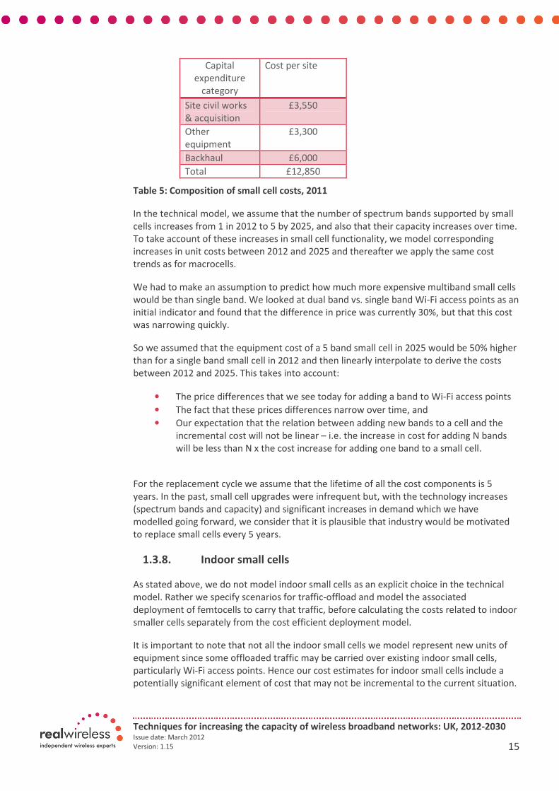
We estimated capital expenditure similarly to macrocells, i.e. we identified 12 separate cost
elements which we grouped into the following categories below and as shown in Table 5:
• Site acquisition and civil works
• Antennas
• Other base station equipment
• Backhaul
Techniques for increasing the capacity of wireless broadband networks: UK, 2012-2030 Issue date: March 2012
Version: 1.15 15
Capital
expenditure
category
Cost per site
Site civil works
& acquisition
£3,550
Other
equipment
£3,300
Backhaul £6,000
Total £12,850
Table 5: Composition of small cell costs, 2011
In the technical model, we assume that the number of spectrum bands supported by small
cells increases from 1 in 2012 to 5 by 2025, and also that their capacity increases over time.
To take account of these increases in small cell functionality, we model corresponding
increases in unit costs between 2012 and 2025 and thereafter we apply the same cost
trends as for macrocells.
We had to make an assumption to predict how much more expensive multiband small cells
would be than single band. We looked at dual band vs. single band Wi-Fi access points as an
initial indicator and found that the difference in price was currently 30%, but that this cost
was narrowing quickly.
So we assumed that the equipment cost of a 5 band small cell in 2025 would be 50% higher
than for a single band small cell in 2012 and then linearly interpolate to derive the costs
between 2012 and 2025. This takes into account:
• The price differences that we see today for adding a band to Wi-Fi access points
• The fact that these prices differences narrow over time, and
• Our expectation that the relation between adding new bands to a cell and the
incremental cost will not be linear – i.e. the increase in cost for adding N bands
will be less than N x the cost increase for adding one band to a small cell.
For the replacement cycle we assume that the lifetime of all the cost components is 5
years. In the past, small cell upgrades were infrequent but, with the technology increases
(spectrum bands and capacity) and significant increases in demand which we have
modelled going forward, we consider that it is plausible that industry would be motivated
to replace small cells every 5 years.
1.3.8. Indoor small cells
As stated above, we do not model indoor small cells as an explicit choice in the technical
model. Rather we specify scenarios for traffic-offload and model the associated
deployment of femtocells to carry that traffic, before calculating the costs related to indoor
smaller cells separately from the cost efficient deployment model.
It is important to note that not all the indoor small cells we model represent new units of
equipment since some offloaded traffic may be carried over existing indoor small cells,
particularly Wi-Fi access points. Hence our cost estimates for indoor small cells include a
potentially significant element of cost that may not be incremental to the current situation.

Techniques for increasing the capacity of wireless broadband networks: UK, 2012-2030 Issue date: March 2012
Version: 1.15 16
We produce separate estimates for enterprise and residential indoor smaller cells, however
we first set out some common assumptions before detailing those specific to enterprise or
residential femtocells.
We model the capital cost of the indoor smalls, but we assume operating expenses are
bundled up into capital costs so we do not calculate them explicitly.
We assume that the extent to which users need to upgrade their fixed broadband
connection is likely to be limited. In particular, mobile broadband use is likely to substitute
for fixed broadband use and may even require less capacity, e.g. video will be scaled down
for viewing on a smart phone screen as opposed to a laptop or PC screen. Hence, we
decided not to attribute broadband costs to femtocell usage.
The final common assumption concerns the equipment lifetime. We assume this is 3 years
on the basis that 3 years appears to be a reasonable average for Wi-Fi access points and
mobile devices, experience of which is likely to condition consumers’ expectations in terms
of the upgrade of femtocells. Further, Signals Research Group4 assume a lifetime of three
years in their femtocell business case study of 2010.
Residential
Currently only HSPA femtocells can be used in the UK, however from 2014, it is reasonable
to assume that operators will want to make available dual mode HSPA/LTE femtocells. We
put together a simple forecast of HSPA only and HSPA/LTE femtocells to examine the
impact on prices.
• HSPA only – Over the past 3 years we have seen HSPA femtocell costs have fallen
by a factor of 3 to below £100 in volume today6. After discussions with industry
sources, we concluded that it was reasonable to assume that the cost could fall
to around 150% of a Wi-Fi access point (today around £50) in another 3 years to
2014 and then at the same annual rate as our standard assumption for radio
equipment. We think that femtocells will not reach quite the same level as Wi-Fi
access points over the course of the model because they are unlikely to achieve
the same production volumes and scale economies and because of additional IPR
costs.
• HSPA/LTE – We reviewed a number of sources7 and concluded that £250 is a
reasonable estimate of the current cost. However, after discussion with industry
sources, we concluded that HSPA/LTE femtocells are not likely to have a
significant impact on the average cost of residential femtocells. This assumes that
production volumes will be low, hence the cost will remain significantly higher
than for HSPA femtocells for some time. If our assumption is wrong and there is
substantial take up dual mode femtocells in the residential market, then costs are
likely to converge to the HSPA only level, hence using the HSPA only cost is still
likely to be a reasonable proxy for the whole market.
6 Signals Research Group [4]
7 e.g. Signals Research Group [4]
Techniques for increasing the capacity of wireless broadband networks: UK, 2012-2030 Issue date: March 2012
Version: 1.15 17
Enterprise smaller cells
There is a wide diversity of systems that could be deployed indoors. We distinguish
between special cases such as airports and stadiums which have very particular
requirements that vary greatly and buildings where capacity demand is much more
homogenous and can be modelled more easily.
We assume that the special sites would be served by indoor cells regardless of the demand
or technical scenario, so we model this as offloaded traffic from the public network.
For more standard deployments of enterprise smaller cells, we model a high level
relationship between demand per building and the number of smaller cells needed to serve
that traffic. This takes into account the likelihood that not all building tenants will deploy
femtocells.
We based our estimate of the cost of an enterprise smaller cell on industry research8. This
indicated a figure of £420 in 2012 and we assume that the cost changes at the same rate as
for macrocell equipment in subsequent years.
1.4. High level assessment of benefits and affordability
In order to place our cost results into some context, we want to give a high level indication
of the benefits and the affordability of the networks that may result from our capacity
scenarios.
We decided to assess the potential benefits on two levels, the overall benefit to UK wireless
broadband consumers and the average revenue per consumer which could be used to
check the affordability by comparing against the average cost per consumer. We would like
to emphasise that this analysis should be regarded as indicative. We have taken a high level
approach partly because the main focus of the study was the costs of meeting wireless
broadband capacity demand and partly because of the inherent difficulties in measuring
the future consumer benefits and revenues for wireless broadband services which are
typically very difficult to predict over the long term that is the focus of this study.
8 Signals Research Group [4]

Techniques for increasing the capacity of wireless broadband networks: UK, 2012-2030 Issue date: March 2012
Version: 1.15 18
1.4.1. Methodology for affordability
Figure 1-5 below gives an overview of the approach we take to examine the affordability of
our scenarios.
Figure 1-5: Approach to assessing affordability
The key to devising the check on costs was to find a total cost per unit measure (over a
relevant period) that could provide a useful comparison with current average revenues per
residential subscriber for mobile services today. Similarly to the assessment of the scenario
costs, we consider only those costs incremental to the existing network.
We decided to calculate the total cost per relevant user within each study area. We take
the sum of the “mobile active” and “working” populations, as defined in our demand model
because these are the users who generate the traffic to which network capacity is
dimensioned.
We estimate the average cost per user over the full period of the model from 2012 to 2030
to produce an average monthly cost. Our costs in in present value terms, so the
affordability comparator (average monthly revenue per user or willingness to pay) needs to
be converted to the same basis, i.e. an average of the present value from 2012 to 2030.
Since access network costs are a fraction of total revenues (between 50-60%), the measure
we use to judge affordability, e.g. the average monthly revenue per user is currently
between £10-15 per month5 depending on how it is measured needs to be scaled by the
same amount. The affordability threshold also needs to be adjusted by a factor to cover the
discounting of the network costs. We discount costs using a social discount rate of 3.5%6.
Over the course of 18 years, a fixed annual amount ‘X’ discounted at this rate and then
averaged over this period would be 25% lower. Applying both these factors to the £10-15
monthly revenue gives a comparative range of about £4-6 which can be compared with the
average monthly cost estimated from the model.
Mobile active +
working population
= Number of relevant
users in each study
area
Total Costs Total Cost per
relevant user
Residential ARPU*
mobile
Residential ARPU
broadband
Mobile broadband
WTP*
(Scaled by ratio of
network costs to
revenues)
*Average revenue per user
**Willingness to pay
Affordability test

Techniques for increasing the capacity of wireless broadband networks: UK, 2012-2030 Issue date: March 2012
Version: 1.15 19
1.4.2. Benefits to consumers
Economists measure consumer benefits by consumer surplus, however it is usually not
straightforward to estimate because it depends on data such as willingness to pay for
wireless broadband services which are not easy to gather or to forecast future levels.
As a result, we have decided to produce a high level estimate the potential benefits to UK
consumers in our analysis through an indirect assessment of consumer surplus for wireless
broadband services.
Our approach is to use existing figures for mobile broadband consumer surplus per
subscriber and apply that to the number of main handset subscriptions that we derive as
explained above in the assessment of affordability. This allows us to estimate a total UK
consumer surplus for wireless broadband use. We estimate this for each year in the model
and calculate the present value of the total in 2012 terms.
Our source for mobile consumer surplus is the Europe Economics study7 for Ofcom. They
estimated consumer surplus from cellular mobile usage at £18 billion for 2006. We divided
this by the number of active mobile subscriptions in 2006 [Ofcom, 5] to get an estimate of
£272 (£23/month) for consumer surplus per mobile subscription.
We assumed that consumer surplus would increase by 2% p.a. due the impact of increased
functionality and falls in the price per unit of demand. Average spending on a basket of
mobile services fell 2.2% p.a. from 2005 to 2010 [Ofcom, 5]. Hence, we conservatively
assumed a similarly sized increase of 2% p.a. in the average consumer surplus per
subscription. This gave a figure of £306 (£25.5/month) for 2012 which we continued to
project forward at a 2% p.a.
We then applied this adjusted consumer surplus figure to the forecast number of main
handset subscriptions and calculated the present value using a social discount rate of 3.5% ,
see HM Treasury [6], from 2012 to 2030 of consumer surplus at £340 billion.

Techniques for increasing the capacity of wireless broadband networks: UK, 2012-2030 Issue date: March 2012
Version: 1.15 20
A2. Technology Considerations and Spectral Efficiency
2.1. Overview of Technology Characterisation by Spectral Efficiency
In this annex we describe the techniques that can be used to increase the efficiency of
mobile broadband delivery, and the method and assumptions used to combine the wide
range of surveyed results into a numerical model for use in this study.
Spectral efficiency is a measure of how well mobile broadband infrastructure technology
exploits each hertz of spectral resource to deliver bits per second of capacity. The units of
our spectral efficiency metric are bits per second of capacity, per hertz of spectrum, per
operator ‘site’. This differs from the more normally used capacity metric of cell spectral
efficiency, since we incorporate the number of cells (or sectors) at the site.
2.2. Capacity Enhancing Techniques
In this section we describe the following capacity enhancing techniques to be included in
the numerical model for spectral efficiency evolution
• Additional Antennas: Sectorisation and MIMO
• MIMO Algorithm Evolution
• Co-ordinated Multipoint
• Small Cells and Offload
• Relays
2.2.1. Additional Antennas: Sectorisation and MIMO
Along with sectorisation, MIMO is one of the main techniques for significantly increasing
spectral efficiency. As a general rule network capacity is proportional to the number of
transmitters. Multiple antennas can be used to create multiple cells or sectors, and they
can also be used to create multiple ‘MIMO layers’. Whether sectors or MIMO layers, the
idea is re-use the spectral resource multiple times from the same cell site. Provided these
are orthogonal and do not interfere with each other, capacity will increase linearly. In
practice, sector overlap and real world channel conditions and antenna designs do result in
adjacent sector or cross layer interference, and the returns for increasing numbers of
antennas are diminishing.
We explicitly model the operator’s decision for the number of downlink transmit antennas
at the macrocell site, either 2, 4 or 8.
• More antennas gives higher spectral efficiency, but incurs higher site costs
• Doubling the number of antennas does not quite double the spectral efficiency,
since the principle of diminishing returns applies.
• Higher order MIMO modes are not supported by the standards until later
generations
• Number of cell site antennas is also taken into account for uplink range
calculations

Techniques for increasing the capacity of wireless broadband networks: UK, 2012-2030 Issue date: March 2012
Version: 1.15 21
The number of UE antennas varies over time according to the device mix. We consider an
evolving mix of 2, 4, and 8 antenna elements in the device. Whilst 8 antenna sites and
devices results in the highest spectral efficiency, deployment will be constrained in practice
by both cost and available space at the site or device
2.2.2. MIMO Algorithm Evolution
LTE-Advanced (i.e. 3GPP Release 10 and beyond) and later generations introduce the
following MIMO enhancements over LTE release 8:
Downlink:
• Up to 8 layer transmission enables the use of up to 8 antennas at the eNodeB,
which can increase peak rates and/or spectral efficiency given suitable antennas
and propagation conditions. Higher numbers of layers are aimed for use in array
antennas, possibly with cross polar elements. E.g. a four beam per sector dual
polar antenna would require 8 layers.
• Multi User MIMO, with fixed or adaptive beams. MU-MIMO enables
transmission for multiple UEs in the same spectral resource at the same time.
This is akin to SDMA (Space Division Multiple Access) where a sector is further
divided into beams, in which the spectral resource can be reused for several
users. MU-MIMO was possible in the Rel8-uplink, and is being added to the
release 10 downlink. MU-MIMO can work with fixed or adaptive beams, where
the latter requires UE specific reference signals that undergo the same pre-
coding as the user traffic. UE specific Reference signals enables correct evaluation
of channel state information at the UE. It is expected that adaptive beam MU
MIMO will bring higher capacity.
• Network MIMO: another name for CoMP. CoMP and MIMO are closely related
as both involve processing of transmissions and/or reception over multiple
antennas. CoMP can be distinguished by the fact that the multiple antennas are
located at different eNodeBs. MIMO implies multiple antennas at a single
eNodeB, but potentially multiple UEs, as in the case of MU MIMO.
Uplink:
• Single User MIMO. Enables a UE to transmit on multiple layers. Release 8 only
supported a single layer per UE on the uplink (but did support MU-MIMO). This
increases the peak rate that can be achieved at high SINRs
• Up to 4 layers
• MU-MIMO Enhanced with CoMP. CoMP and MIMO are closely related as both
involve
• Single User MIMO up to 4 layers (rel-8 only supported Multi-User MIMO on UL)
• Multi User MIMO enhanced by joint transmission (see CoMP)
Figure 2-1 illustrates the relative benefit of transmit and receive antennas in MIMO
configurations. Doubling the number transmit antennas (1x2 vs. 2x2, or 2x4 vs 4x4)
improves throughput at higher SINRs only, and so spectral efficiency will only occur in
environments with a prevalence of higher SINR conditions, such as small cells. Increasing

Techniques for increasing the capacity of wireless broadband networks: UK, 2012-2030 Issue date: March 2012
Version: 1.15 22
the number of receive antennas (2x2 vs 2x4) improves throughput across the whole range
of SINR, and should therefore provide capacity gains in any environment.
Figure 2-1: Single User MIMO Benefits. Source 3G Americas8, Real Wireless graph
In addition to SINR, suitable combinations of multipath conditions and antennas are also
required to ensure that the channel can be ‘decomposed’ into orthogonal propagation
modes. This generally requires rich multipath scattering, although it should be noted that
dual polar MIMO can provide orthogonal propagation modes without the need for
scattering. MIMO channel and antenna combinations can be characterised by matrix
parameters such as ‘rank’ which indicates the number of layers that can be supported and
‘condition number’, which indicates how reliably multilayer transmission can be
achieved[9]]. Figure 2-2 illustrates the prevalence of multilayer transmission (ranks higher
than 1) in field trials of 2x2 and 4x4 MIMO with various cross polar antenna configurations.
The impact on the user throughput distribution is also shown. The figure shows the
importance of the UE antenna configuration, with the dual polar UE (labelled |-) achieving
rank 2 significantly more than the single polar UE (||). Similar trends can be seen with the
4x4 configuration. Of note also is that the prevalence of rank 4 transmission is very low,
occurring in only 1 or 2% of locations in the cell. This does not mean that 4x4
configurations are of no value, as significant throughput benefits can still be observed over
2x2. The 4x4 configurations have a higher prevalence of multi layer transmission (rank>1)
than 2x2 configurations. Other trials results in an Ericsson paper[10
] showed that 4x4
increased average user throughput by 50% compared to 2x2. This is indicative of the gains
in cell spectral efficiency that could be achieved, and aligns well with simulation results
shown later in Figure 2-4.
0
1
2
3
4
5
6
7
8
-20 -10 0 10 20 30
Lin
k L
ev
el
Pe
rfo
rma
nce
,
bp
s/H
z/u
ser
SINR, dB
4x4
2x4
2x2
1x2

Techniques for increasing the capacity of wireless broadband networks: UK, 2012-2030 Issue date: March 2012
Version: 1.15 23
Figure 2-2: Prevalence of Multilayer Transmission in MIMO Propagation Trials. Copied
from Ericsson Review11. Note that x indicates a cross polar eNodeB antenna, and | and –
indicate vertical and horizontal UE antennas.
Figure 2-3: Benefit of LTE-Advanced DL MIMO Schemes over LTE Rel. 8 4x2. Source:
3GPP[12
], Real Wireless analysis. Assumes eNodeB antenna configurations of |||| and
XXXX for 4 and 8 way tx, respectively.
Figure 2-3 summarises the benefits of the LTE-Advanced MIMO schemes over a baseline
Release 8 SU-MIMO 4x2 scheme, in both Macrocell and Microcell environments. The 4x2
configurations show the benefit of the enhanced MIMO processing is around 30-50%.
Doubling the number of transmit antennas to 8 brings further gains, especially in the
macrocell environment. This is the reverse of the mechanism seen in Figure 2-1, where Tx
antennas provided more gain in higher SINR environments. This may be because in this
case, the number of Tx antennas (8) greatly exceeds the Rx (2).
0
43
% 51
%
47
%
68
%
92
%
12
0%
0
32
%
43
% 52
% 60
% 64
% 75
%
0%
20%
40%
60%
80%
100%
120%
140%
R8 SU-
MIMO
MU-MIMO CS/CB
CoMP
JP-CoMP MU-MIMO CS/CB
CoMP
SU-MIMO
4x2 8x2
Be
ne
fit
to C
ell
SE
ov
er
R8
SU
MIM
O 4
x2
ITU Macrocell
ITU Microcell

Techniques for increasing the capacity of wireless broadband networks: UK, 2012-2030 Issue date: March 2012
Version: 1.15 24
Figure 2-4 illustrates the benefits of higher order MIMO configurations with Rel 8 SU
MIMO, as well as LTE-Advanced MU-MIMO and CoMP schemes. As before, we see that LTE-
Advanced schemes are able to extract more benefit from the higher order schemes, with
4x4 JP CoMP achieving almost 2x the spectral efficiency as the 2x2 equivalent. The same
antenna upgrade with Rel8 MIMO would only have brought 1.5x benefit.
Figure 2-4: Benefit of higher order MIMO schemes over 2x2, 3GPP Macrocells. Source
3GPP[13
], Real Wireless analysis.
Enhanced MIMO processing in LTE-Advanced can enhance the performance of a given
MIMO configuration by 20-50%, with greater benefits for 4tx configurations than for 2tx.
Increasing the number of antennas generally improves spectral efficiency. Both Trials and
simulations of Rel 8 LTE indicate a 50% increase in cell spectrum efficiency is achieved with
4x4 compared to 2x2. With LTE Advanced schemes, up to 2x benefit could be achieved by
doubling the number of antennas at both ends of the link. Upgrading the eNodeB to 8
antennas can bring further gains. 8x2 SU-MIMO gave over 2x the cell SE compared to the
same scheme with 4x2 configurations.
Challenges
• It is difficult to design multiple diverse antennas on small form factor terminals,
especially at low frequencies, see Varall 14
• MIMO cell site antennas may need to be larger, increasing site leasing costs
• MIMO requires high SINR and rich scattering. If this combination of conditions
does not occur very often in the target environment, then benefits will be low.
0%
10%
20%
30%
40%
50%
60%
70%
80%
90%
100%
2x2 4x2 4x4
Ce
ll S
E b
en
efi
t o
ve
r 2
x2
Rel 8 SU MIMO
MU MIMO
JP CoMP

Techniques for increasing the capacity of wireless broadband networks: UK, 2012-2030 Issue date: March 2012
Version: 1.15 25
Capacity Gains from MIMO
• Increasing the number of receive antennas in a MIMO configuration increases
spectral efficiency
• Increasing the number of transmit antennas increases peak rates at high SINR,
but will only increase spectral efficiency if higher SINRs are prevalent in the
environment. Small cell environments tend to have higher SINRs, hence greater
MIMO benefits.
• MIMO Gains may be greater at higher carrier frequencies, where the smaller
wavelength facilitates better antenna design for a given form factor.
Numerical Model for MIMO
Our site spectral efficiency figures represent an evolving mix of practical MIMO technology:
• HSPA+ provides MIMO, but the challenges of channel estimation for CDMA limit
its efficacy.
• Release 8 LTE provides up to 4 layer single user MIMO on the downlink
• Release 10 increases to 8 layer, and support of Multi-User MIMO.
• MU-MIMO in release 10 combined with a closely spaced array antenna is akin to
beamforming
• In practice, MIMO gains are limited by antenna correlation and presence of
suitable scattering in the propagation environment.
• Our prediction for releases 12 and beyond considers further potential for
algorithm enhancement depending on the technology scenario.
2.2.3. Co-ordinated Multi Point (CoMP)
In a cellular network, most UEs can hear (or be heard) by more than one cell. In a basic
system, we consider the strongest signal to be the serving cell, and all others to be
interferers. The premise of CoMP (Co-ordinated MultiPoint) is that cells share information
to either reduce other cell interference or harness it to improve network capacity. Figure
2-5 illustrates the key concepts of CoMP. In LTE, the X2 is an optional interface between
eNodeBs which can be used for co-ordination.
Figure 2-5: Co-ordinated Multipoint Transmission Concepts

Techniques for increasing the capacity of wireless broadband networks: UK, 2012-2030 Issue date: March 2012
Version: 1.15 26
We can imagine that the highest uplink theoretical capacity could be achieved by sending
all the complex voltage waveforms received on each antenna element of all base stations to
a massive central processing unit. This could extract and combine signals from each UE as
well as cancelling known interference from other UEs. Similarly on the downlink, signals for
all UEs could be optimally transmitted from all eNodes taking into account all complex
channel responses of all UEs. In practice this approach would not be viable as the backhaul,
synchronisation and processing requirements would be prohibitive. However, schemes
have and are being specified for LTE and LTE-Advanced which can achieve some of the
benefits with practical levels of information exchange and processing. These largely fall
into two groups as follows:
1) Joint Processing (JP): A UE can have multiple serving cells, requiring user data to be
transmitted (or received) in multiple locations. This requires sharing of both scheduling
information and the users’ data between neighbour cells.
2) Co-ordinated Scheduling (CS): A UE only has one serving cell, so no sharing of user
data is required. Scheduling information is shared between neighbour cells in order to
avoid or reduce interference. Scheduling information could be power levels per resource
block, load levels, beamforming weights, etc. CS schemes require less information sharing
and processing than JP, but do not in general achieve such high potential capacity gains.
Figure 2-6 Intra and Inter eNodeB CoMP
The benefits of CoMP come at the expense of information sharing between cells. Such
sharing is not always a problem as illustrated by the three scenarios in Figure 2-6.
1) UE1 sits near the edge of two cells around the same eNodeB so information
exchange will be internal and thus can more easily be high bandwidth and synchronised.
2) CoMP for UE2 would be inter eNodeB, requiring the use of backhaul bandwidth on
the X2 interface for information sharing. Latency on this interface impacts performance as
described later.
3) UE 3 uses intra eNodeB CoMP between different Remote Radio heads. Since these
are linked to their controlling eNodeB with the OBRI interface (a digitised baseband
waveform), CoMP does not impact the bandwidth requirement.
UE2UE1
UE3
b) Distributed eNodeB
X2 interface
Remote
Radio Heads
a) Tri-sector eNodeB
CoMP scenarios
UE1 Intra eNodeB
UE2 Inter eNodeB over X2
UE3 Intra eNodeB over OBRI
OBRI interface
(fibre)
Techniques for increasing the capacity of wireless broadband networks: UK, 2012-2030 Issue date: March 2012
Version: 1.15 27
Furthermore it should be noted that intra eNodeB CoMP can use proprietary algorithms,
whereas inter-eNodeB needs to be standardised to work in a multi-vendor environment.
The following sections outline the downlink and uplink schemes being standardised for LTE.

Techniques for increasing the capacity of wireless broadband networks: UK, 2012-2030 Issue date: March 2012
Version: 1.15 28
2.2.3.1. Downlink CoMP
Inter-Cell Interference Co-ordination (ICIC)
ICIC is a simple CoMP scheme that was standardised in rel-8 LTE. This falls under the co-
ordinated scheduling category, as each UE has one serving cell. Figure 2-7 illustrates a
scenario where co-ordination improves capacity. The diagrams show two cells each serving
one user. In a) both UEs are near to their cells, so the wanted signal is much stronger than
the interfering signal. Maximum capacity is achieved by both cells transmitting maximum
power. In scenario b), the UEs are near the cell edge, so the wanted and interfering signals
are at similar levels. Working individually, each cell could maximise its UE throughput by
transmitting more power. However the combined capacity will be higher if they co-
ordinate so that only one of the cells transmits at a time (on a given frequency) and the
other transmits nothing[15
].
Figure 2-7: Scenarios to illustrate benefit of Inter cell Co-ordination
In practice this can be achieved by categorising UEs as either cell-centre or cell-edge, and
schedulers in adjacent cells co-ordinating to ensure no two adjacent cell edge UEs transmit
on the same frequency resource as illustrated in Figure 2-8. In this example, cell centre UEs
have N=1 reuse (all cells reuse the same frequency resource), whereas the cell edge is
effectively N=3 reuse, where each cell edge region can only use a third of the spectrum.
This is similar to the frequency reuse patterns used in early 2G networks (before frequency
hopping), where the reuse factor allows a trade between cell capacity and cell edge
performance.
The reader should be aware that in a real world propagation environment with terrain and
clutter, the division between cell edge and centre would not be as neat as that shown in
Figure 2-8. The criteron for deciding whether a UE is cell edge or centre would be based on
signal strength/quality rather than its geographical location relative to the cell sites.
Techniques for increasing the capacity of wireless broadband networks: UK, 2012-2030 Issue date: March 2012
Version: 1.15 29
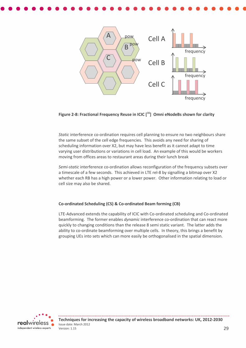
Figure 2-8: Fractional Frequency Reuse in ICIC [16
] Omni eNodeBs shown for clarity
Static interference co-ordination requires cell planning to ensure no two neighbours share
the same subset of the cell edge frequencies. This avoids any need for sharing of
scheduling information over X2, but may have less benefit as it cannot adapt to time
varying user distributions or variations in cell load. An example of this would be workers
moving from offices areas to restaurant areas during their lunch break
Semi-static interference co-ordination allows reconfiguration of the frequency subsets over
a timescale of a few seconds. This achieved in LTE rel-8 by signalling a bitmap over X2
whether each RB has a high power or a lower power. Other information relating to load or
cell size may also be shared.
Co-ordinated Scheduling (CS) & Co-ordinated Beam forming (CB)
LTE-Advanced extends the capability of ICIC with Co-ordinated scheduling and Co-ordinated
beamforming. The former enables dynamic interference co-ordination that can react more
quickly to changing conditions than the release 8 semi static variant. The latter adds the
ability to co-ordinate beamforming over multiple cells. In theory, this brings a benefit by
grouping UEs into sets which can more easily be orthogonalised in the spatial dimension.
Cell A
B
C
frequency
pow
Cell B
frequency
pow
Cell C
frequency
pow
A
Techniques for increasing the capacity of wireless broadband networks: UK, 2012-2030 Issue date: March 2012
Version: 1.15 30
Joint Processing Techniques
Joint Processing category requires the user’s data to be present at multiple cells in the
‘CoMP Cooperation Set’. There are two JP variants proposed for LTE-A: Dynamic Cell
Selection and Joint Transmission.
i) Dynamic Cell Selection is akin to fast macro diversity: User data is present in all
cells in the Coordination set, but is only transmitted from one cell at a time. The
transmission cell can be rapidly changed on a per 1ms subframe basis, depending on
channel conditions, cell load, etc. This is like a very fast handover
ii) Joint Transmission is where multiple cells simultaneously transmit data to the user.
The multiple signals are co-ordinated such that they arrive at the UE to improve the
strength of the wanted signal, or actively cancel interference from other UEs.
Transmissions can be coherent or non-coherent. Coherent transmissions can improve the
signal quality more, but require very tight synchronisation which is difficult to achieve for
cells at different sites
Joint transmission is a type of network MIMO, where the multiple transmit antennas can be
located at different cell sites, rather than an array antenna at a single cell site. The network
uses the multiple cell sites to form ‘beams’ to particular UEs, whilst nulling out others. JT
can also be used in conjunction with Multi-User MIMO, where the multiple receive
antennas can be located on different UEs. This allows the network to reuse the same
(frequency, time) resource to send different information to multiple users.
Further details of the CoMP schemes and the signalling to support them can be found in TR
36.813 [17
]
2.2.3.2. Uplink CoMP
Both Joint Processing and Co-ordinated Scheduling schemes are possible on the uplink.
Co-ordinated Scheduling and Beamforming
Since the scheduler for both uplink and downlink resides in the eNodeB, co-ordination
mechanisms are similar for both. In LTE rel-8, eNodeBs can share information on which
resources they have scheduled high power uplink transmissions. They can also share
reports of strong uplink interference which helps eNodeBs work out which UEs have strong
signal paths to their neighbour cells, and thus need to be co-ordinated. LTE-Advanced
extends the capabilities to include co-ordination over shorter timescales and over UE
beamforming.
Joint Reception
The UE signal may be received at multiple cells and then recombined to reduce errors or
packet loss. The degree of coherency depends on whether the cells are controlled by the
same eNodeB, or whether user data must be sent over the backhaul between different
eNodeBs.
Uplink CoMP is predominantly a function of the eNodeB scheduler and so little
standardisation is needed as this can be left to vendor implementation. Specifications will
however be needed for measurements and signalling needed to support UL CoMP.

Techniques for increasing the capacity of wireless broadband networks: UK, 2012-2030 Issue date: March 2012
Version: 1.15 31
2.1.1.1 Benefits of CoMP
Various different opinions exist on the extent of the benefits of CoMP.
Results of the 3GPP feasibility study show clear benefits to downlink cell spectrum
efficiency. With 4 tx antennas at the eNodeB, gains of over 30% are achieved with for Co-
ordinated Scheduling and beamforming, and over 50% for Joint Processing CoMP, as shown
in Figure 2-9. Figure 2-10 shows more simulation results with more modest gains in Cell SE
for all but the most sophisticated of schemes. None of the Single User schemes achieve
more than 11% benefit to SE compared to Rel8 LTE. Note that the antenna configuration
has not been stated and a 2x2 configuration would result in lower gains, as shown by the
3GPP results in Figure 2-9
Figure 2-9: Benefit of LTE-Adv DL CoMP Schemes over Rel8 LTE: Source 3GPP Feasibility
Study18, Real Wireless Analysis
Figure 2-10: 3G Americas DL CoMP Simulation Results9 (Source: 3G Americas19
)
9 Coordinated Beam Switching (CBS), Non-Coherent Joint Processing (JP-Nco), Coherent Joint
Processing (JP-Co), Co-ordinated Beamforming (CBF) Intra-Site Coherent JP
0%
10%
20%
30%
40%
50%
60%
2x2 4x2 4x4
Ce
ll S
E b
en
efi
t o
ve
r
Re
l8 S
U M
IMO
CS/CB CoMP
JP CoMP

Techniques for increasing the capacity of wireless broadband networks: UK, 2012-2030 Issue date: March 2012
Version: 1.15 32
Figure 2-10 also shows benefits of CoMP for Cell edge User throughput of around 10-20%
for the single user cases. It is these users with high interference levels that should get the
most benefits of CoMP, and the result should be a fairer network able to guarantee a
higher minimum throughput. Qualcomm results for CoMP shown in Figure 2-11 support
this view, but show that the benefit to cell edge UEs comes at the cost of the 50% and 95%-
ile with median and peak UE throughputs, respectively. These results suggest that CoMP
can alter the shape of the UE Tput distribution, but do not bring a net improvement. The
lack of benefit to the median (50%ile) UE Tput implies that cell spectral efficiency would not
improve. The simulations assumed a 1x2 antenna configuration, which suggests that CoMP
needs to be deployed in combination with MIMO to provide benefits. Figure 2-9 above
showed that higher gains are achieved with the higher order antenna configurations.
Figure 2-11: Qualcomm Paper on Joint Transmission 20 in 1x2 configuration shows that
whilst the proposed schemes improve 5%-ile UE Tputs, they actually degrade median and
95%ile throughput.
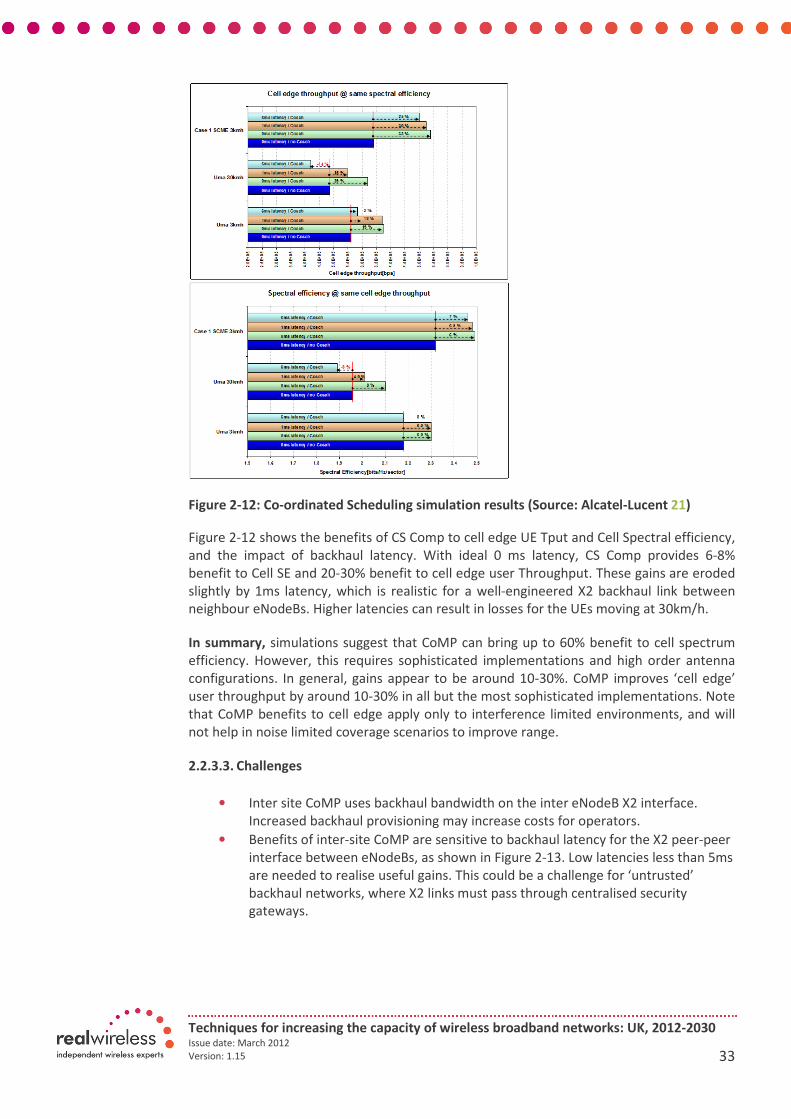
Techniques for increasing the capacity of wireless broadband networks: UK, 2012-2030 Issue date: March 2012
Version: 1.15 33
Figure 2-12: Co-ordinated Scheduling simulation results (Source: Alcatel-Lucent 21)
Figure 2-12 shows the benefits of CS Comp to cell edge UE Tput and Cell Spectral efficiency,
and the impact of backhaul latency. With ideal 0 ms latency, CS Comp provides 6-8%
benefit to Cell SE and 20-30% benefit to cell edge user Throughput. These gains are eroded
slightly by 1ms latency, which is realistic for a well-engineered X2 backhaul link between
neighbour eNodeBs. Higher latencies can result in losses for the UEs moving at 30km/h.
In summary, simulations suggest that CoMP can bring up to 60% benefit to cell spectrum
efficiency. However, this requires sophisticated implementations and high order antenna
configurations. In general, gains appear to be around 10-30%. CoMP improves ‘cell edge’
user throughput by around 10-30% in all but the most sophisticated implementations. Note
that CoMP benefits to cell edge apply only to interference limited environments, and will
not help in noise limited coverage scenarios to improve range.
2.2.3.3. Challenges
• Inter site CoMP uses backhaul bandwidth on the inter eNodeB X2 interface.
Increased backhaul provisioning may increase costs for operators.
• Benefits of inter-site CoMP are sensitive to backhaul latency for the X2 peer-peer
interface between eNodeBs, as shown in Figure 2-13. Low latencies less than 5ms
are needed to realise useful gains. This could be a challenge for ‘untrusted’
backhaul networks, where X2 links must pass through centralised security
gateways.
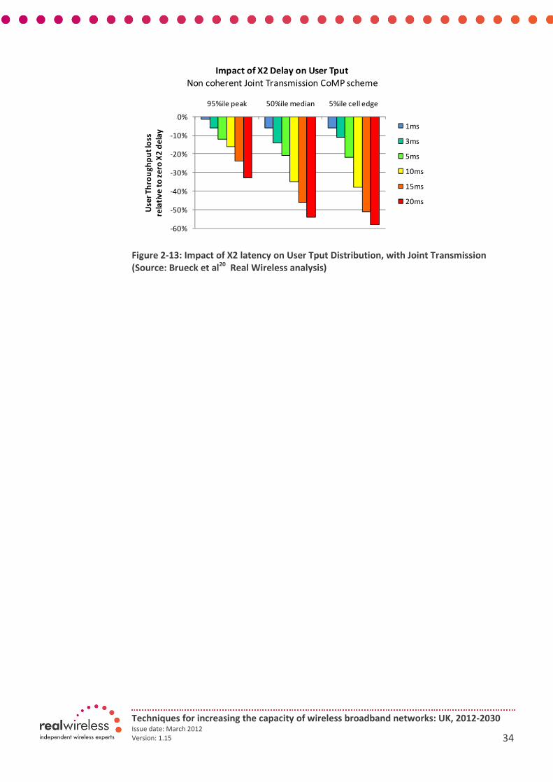
Techniques for increasing the capacity of wireless broadband networks: UK, 2012-2030 Issue date: March 2012
Version: 1.15 34
Figure 2-13: Impact of X2 latency on User Tput Distribution, with Joint Transmission
(Source: Brueck et al20
Real Wireless analysis)
-60%
-50%
-40%
-30%
-20%
-10%
0%
95%ile peak 50%ile median 5%ile cell edge
Use
r T
hro
ug
hp
ut
loss
rela
tiv
e t
o z
ero
X2
de
lay
Impact of X2 Delay on User Tput
Non coherent Joint Transmission CoMP scheme
1ms
3ms
5ms
10ms
15ms
20ms

Techniques for increasing the capacity of wireless broadband networks: UK, 2012-2030 Issue date: March 2012
Version: 1.15 35
2.2.4. Small cells
Two types of small cell are emerging: consumer and enterprise deployed femtocells, and
operator deployed and managed small cells, also referred to as ‘metrocells’ or ‘picocells’.
In this study we refer to these different types of small cells as follows:
Indoor small cells
• Deployment and backhaul managed by consumer or enterprise customer.
• Treated as ‘offload’ by the capacity techniques study, by removing (or reducing)
certain demand points representing indoor demand
Outdoor small cells
• Deployment and backhaul managed by operators.
• Explicitly modelled as a site type with shorter range and generally lower capacity
than macrosites.
The concept behind femtocells is the ability to deploy/extend cellular coverage and capacity
within a residential or small office environment. Femtocells enable consumers to effectively
deploy mobile coverage within their home using the consumers’ broadband connectivity as
the backhaul to the network. Femtocell technology is also being applied to public
environments, overlapping with the traditional application areas of picocells, microcells and
distributed antennas systems.
Coverage normally extends between 10 – 30m from the femtocell access point unit and
typically supports 4- 8 handsets when deployed in a residential environment and 10 -15
handsets within an enterprise environment.
There are some clear advantages and disadvantages for deploying femtocells that support
enhancement for capacity in 4G networks and this is addressed in more detail in the
sections below.
Femtocells in the standards
Femtocells have been added to 3GPP specifications from release 8 and 9 with use of the
terms HNB (for UMTS/HSPA) and HeNB (for LTE). Standardising femtocell technology
creates an enabler for the wide scale deployment and interoperability between global
vendors and operators. For example, GSM, UMTS, HSPA and LTE cellular standards are all
supported on femtocell networks.
The WiMAX Forum is also building femtocells into their standards (see WiMAX Forum
website) and further supports interoperability between different cellular technologies.

Techniques for increasing the capacity of wireless broadband networks: UK, 2012-2030 Issue date: March 2012
Version: 1.15 36
Differences between home and enterprise femtocells
Initially femtocells started off being for coverage in the home but have evolved into
enterprise femtocells to cover larger office areas
Motivation for enterprise femtocells is to:
• Provide coverage more easily in indoor environments
• Offload capacity from the macro layer to small cell architectures
• Improve user experience by providing a better SINR so data rates are better
• Reduce the cost of delivering high quality service to subscribers – papers from
Signals Research Group (SRG) and Small Cell Forum (formerly Femto Forum)
indicate a 4-100 times cost reduction per GB with femtocells compared to
macrocells, depending on the architecture, backhaul and traffic routing adopted
in both the macrocell and femtocell layers [22].
A high level femtocell network architecture is shown in Figure 2-14 which highlights where
the femtocell is situated in the wider (macro layer) network context. The capacity
enhancement takes place due to the dedicated network resource provision with little or no
contention to access the radio network, combined with a typically higher SINR across most
of the cell.
Figure 2-14 High level femtocell network structure Source: Femto Forum 23
2.2.4.1. Benefits
• Enables order of magnitude increase in cell density at realistic costs
• Users self deploy capacity and coverage where they need it
• Reduces load on macro layer, improving service for outdoor high mobility users

Techniques for increasing the capacity of wireless broadband networks: UK, 2012-2030 Issue date: March 2012
Version: 1.15 37
Femtocells bring benefits to both users and operators.
The benefits to users include:
• Enhanced coverage indoors in areas where there may otherwise be poor cellular
coverage
• Enhanced capacity to mobile broadband users, small lightly loaded cells offers
higher data rates (this is dependent on the quality of the broadband connection)
• Attractive tariffs and bundles offered by operators when under femtocell
coverage
The benefits to operators include:
• Offload traffic from macro layer to femtocells reduces the load thus freeing up
capacity to the public network
• Reduced network roll out costs of network including capital and operational
expenditure
The two main benefits of deploying femtocells in relation to capacity enhancements
include:
• Femtocells provide enhancement to capacity
a) Fundamentally femtocells enable spectrum to be reused at a higher density, delivering and increased capacity density which can be matched to hotspots of demand, provided interference between cells can be properly managed.
b) The resulting capacity gains for the network as whole can be large, with for example a gain of around 100 times for a given user throughput indicated in [24
] for 3G.
c) Real-world deployments have now demonstrated femtocells working on the same carrier as macros without interference issues. For example, AT&T have indicated that they are successfully operating femtocells co-channel with both GSM and UMTS macrocells [
25].
• Spectrum efficiency improvements
a) Smaller cells give a better SINR distribution and result in improved spectral efficiency (see chapter 4)
b) Higher channel rank should mean MIMO works better
2.2.4.2. Challenges
Many of the early challenges in femtocell deployment have been overcome. For example
the interference issues that have been highlighted from early deployments have now been
resolved by introducing interference mitigation techniques which enables co-channel
operation between the femtocell and macrocell.[24]. Furthermore, the regulatory
implications for unregulated use of spectrum by a consumer (that does not hold a licence)
has been resolved in many territories, on the basis that the operator retains control of the
femtocell transmission via the authenticated secure tunnel created between the femtocell
and the operator’s core network.
Other challenges of deploying femtocells which can impact upon their use are mainly found
in the use of consumer backhaul. There is a dependence on the consumer/user to have a

Techniques for increasing the capacity of wireless broadband networks: UK, 2012-2030 Issue date: March 2012
Version: 1.15 38
good quality broadband connection in their home or office to realise the key benefits of
femtocells. Other challenges include:
• Ensuring self-deployment and optimisation work on a large scale
• Managing interference between femtocell and macrocell layers
• Ensuring sufficient QoS over DSL backhaul
• Ensuring femtocells are available cost-effectively so as to be attractive to
sufficient numbers of consumers
2.2.4.3. Numerical Model
Indoor small cells are modelled as offload, utilising a network architecture of the form
shown in Figure 2-15: Range is not modelled, rather an indoor small cell reduces or
removes an amount of indoor demand at a single demand point (i.e. postal address). Small
cell spectral efficiency is slightly higher than that of macrocells due to the improved
isolation from neighbour cell interference. The number of bands and bandwidths per band
supported is limited given the constraints of the small form factors required. Details and
assumptions are described later
Outdoor small cells are modelled explicitly in much the same way as macrocell sites, albeit
with reduced range and site spectral efficiency. The number of bands supported is also
limited, given form factor constraints.
Figure 2-15: Offload for the Access and Core Networks (offload can occur at the access
point or at the gateway depending on the configuration).
2.2.5. Relaying
Relays can be deployed in a number of scenarios to improve performance. They can be
used to extend coverage and/or improve data rates in areas which would otherwise low
signal quality. Other applications are temporary sites (at events, or in emergency
scenarios), or on a moving vehicle such as train, to improve link stability and handle ‘group
handover’. Relays might also be used during initial roll out to reduce costs of installing
dedicate bandwidth to each eNodeB. A relay can be ‘upgraded ‘ to a eNodeB when justified
by capacity demand .
Radio Access Network Core Internet
Access Offload:
Femtocells, WiFi, etc
Gateway
Core Offload
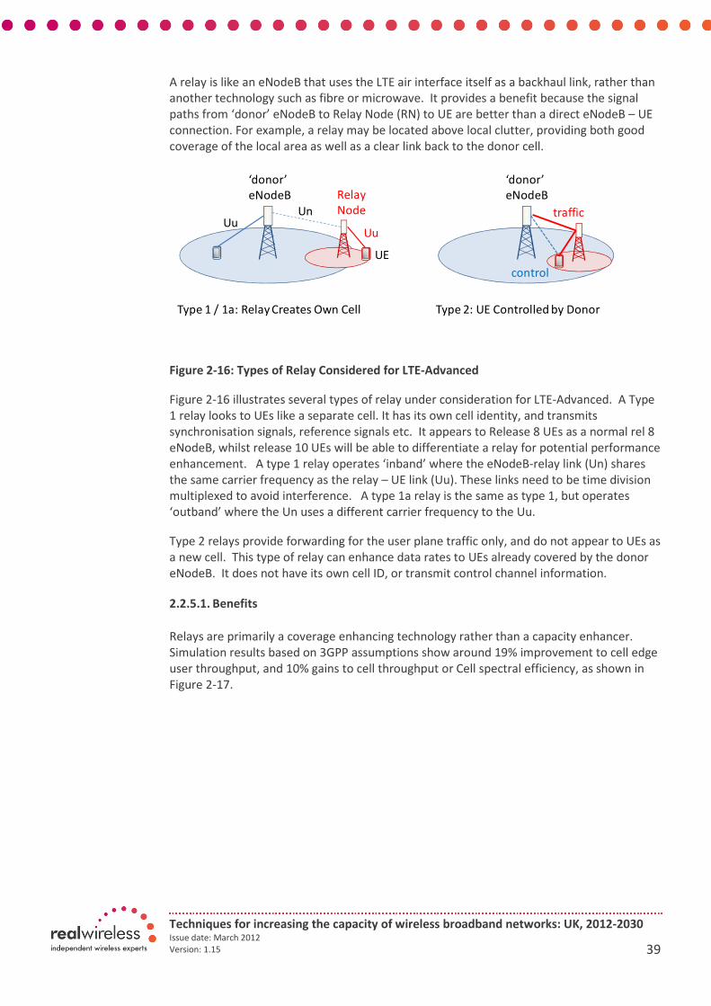
Techniques for increasing the capacity of wireless broadband networks: UK, 2012-2030 Issue date: March 2012
Version: 1.15 39
A relay is like an eNodeB that uses the LTE air interface itself as a backhaul link, rather than
another technology such as fibre or microwave. It provides a benefit because the signal
paths from ‘donor’ eNodeB to Relay Node (RN) to UE are better than a direct eNodeB – UE
connection. For example, a relay may be located above local clutter, providing both good
coverage of the local area as well as a clear link back to the donor cell.
Figure 2-16: Types of Relay Considered for LTE-Advanced
Figure 2-16 illustrates several types of relay under consideration for LTE-Advanced. A Type
1 relay looks to UEs like a separate cell. It has its own cell identity, and transmits
synchronisation signals, reference signals etc. It appears to Release 8 UEs as a normal rel 8
eNodeB, whilst release 10 UEs will be able to differentiate a relay for potential performance
enhancement. A type 1 relay operates ‘inband’ where the eNodeB-relay link (Un) shares
the same carrier frequency as the relay – UE link (Uu). These links need to be time division
multiplexed to avoid interference. A type 1a relay is the same as type 1, but operates
‘outband’ where the Un uses a different carrier frequency to the Uu.
Type 2 relays provide forwarding for the user plane traffic only, and do not appear to UEs as
a new cell. This type of relay can enhance data rates to UEs already covered by the donor
eNodeB. It does not have its own cell ID, or transmit control channel information.
2.2.5.1. Benefits
Relays are primarily a coverage enhancing technology rather than a capacity enhancer.
Simulation results based on 3GPP assumptions show around 19% improvement to cell edge
user throughput, and 10% gains to cell throughput or Cell spectral efficiency, as shown in
Figure 2-17.
Type 1 / 1a: Relay Creates Own Cell
UuUn
‘donor’
eNodeB Relay
Node
Uu
UE
Type 2: UE Controlled by Donor
traffic
control
‘donor’
eNodeB
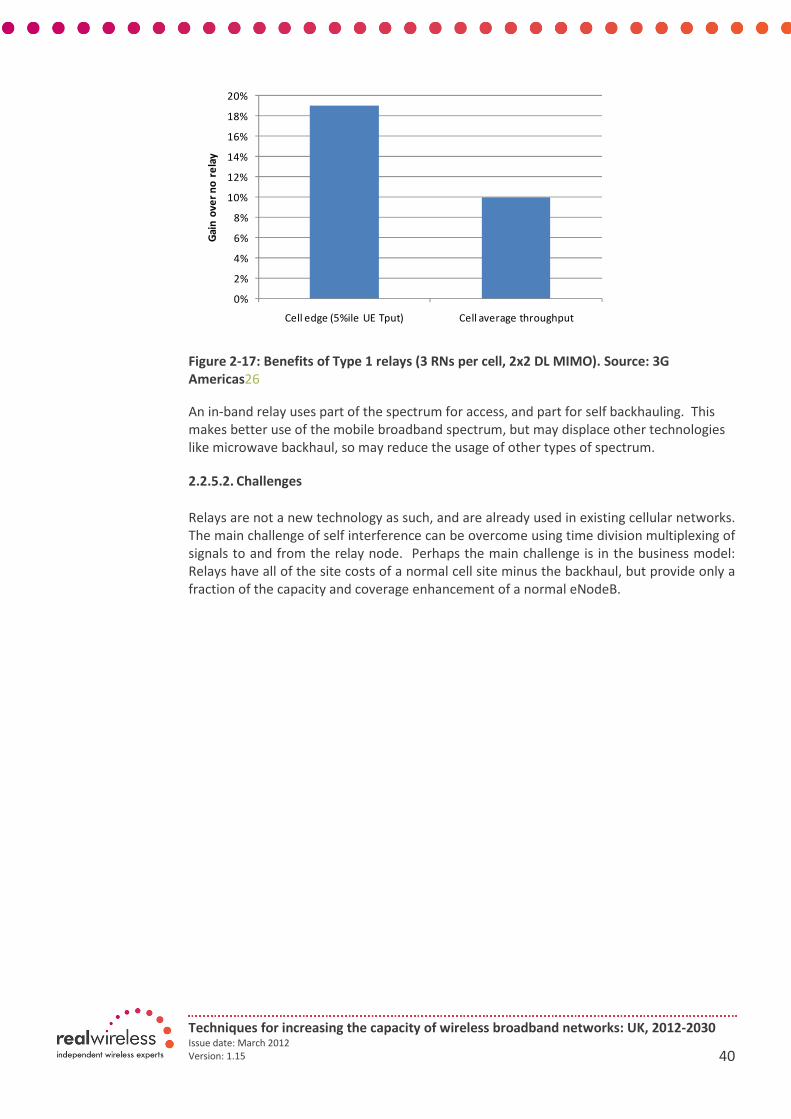
Techniques for increasing the capacity of wireless broadband networks: UK, 2012-2030 Issue date: March 2012
Version: 1.15 40
Figure 2-17: Benefits of Type 1 relays (3 RNs per cell, 2x2 DL MIMO). Source: 3G
Americas26
An in-band relay uses part of the spectrum for access, and part for self backhauling. This
makes better use of the mobile broadband spectrum, but may displace other technologies
like microwave backhaul, so may reduce the usage of other types of spectrum.
2.2.5.2. Challenges
Relays are not a new technology as such, and are already used in existing cellular networks.
The main challenge of self interference can be overcome using time division multiplexing of
signals to and from the relay node. Perhaps the main challenge is in the business model:
Relays have all of the site costs of a normal cell site minus the backhaul, but provide only a
fraction of the capacity and coverage enhancement of a normal eNodeB.
0%
2%
4%
6%
8%
10%
12%
14%
16%
18%
20%
Cell edge (5%ile UE Tput) Cell average throughput
Ga
in o
ve
r n
o r
ela
y
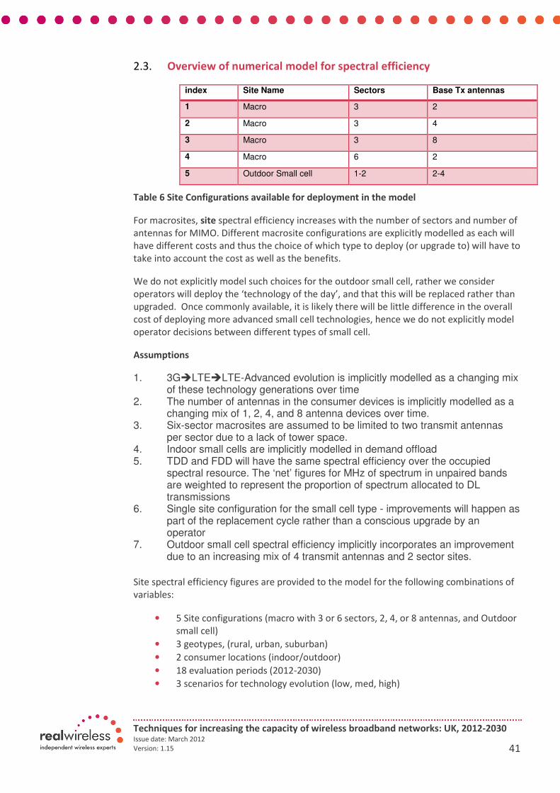
Techniques for increasing the capacity of wireless broadband networks: UK, 2012-2030 Issue date: March 2012
Version: 1.15 41
2.3. Overview of numerical model for spectral efficiency
index Site Name Sectors Base Tx antennas
1 Macro 3 2
2 Macro 3 4
3 Macro 3 8
4 Macro 6 2
5 Outdoor Small cell 1-2 2-4
Table 6 Site Configurations available for deployment in the model
For macrosites, site spectral efficiency increases with the number of sectors and number of
antennas for MIMO. Different macrosite configurations are explicitly modelled as each will
have different costs and thus the choice of which type to deploy (or upgrade to) will have to
take into account the cost as well as the benefits.
We do not explicitly model such choices for the outdoor small cell, rather we consider
operators will deploy the ‘technology of the day’, and that this will be replaced rather than
upgraded. Once commonly available, it is likely there will be little difference in the overall
cost of deploying more advanced small cell technologies, hence we do not explicitly model
operator decisions between different types of small cell.
Assumptions
1. 3G�LTE�LTE-Advanced evolution is implicitly modelled as a changing mix of these technology generations over time
2. The number of antennas in the consumer devices is implicitly modelled as a changing mix of 1, 2, 4, and 8 antenna devices over time.
3. Six-sector macrosites are assumed to be limited to two transmit antennas per sector due to a lack of tower space.
4. Indoor small cells are implicitly modelled in demand offload 5. TDD and FDD will have the same spectral efficiency over the occupied
spectral resource. The ‘net’ figures for MHz of spectrum in unpaired bands are weighted to represent the proportion of spectrum allocated to DL transmissions
6. Single site configuration for the small cell type - improvements will happen as part of the replacement cycle rather than a conscious upgrade by an operator
7. Outdoor small cell spectral efficiency implicitly incorporates an improvement due to an increasing mix of 4 transmit antennas and 2 sector sites.
Site spectral efficiency figures are provided to the model for the following combinations of
variables:
• 5 Site configurations (macro with 3 or 6 sectors, 2, 4, or 8 antennas, and Outdoor
small cell)
• 3 geotypes, (rural, urban, suburban)
• 2 consumer locations (indoor/outdoor)
• 18 evaluation periods (2012-2030)
• 3 scenarios for technology evolution (low, med, high)
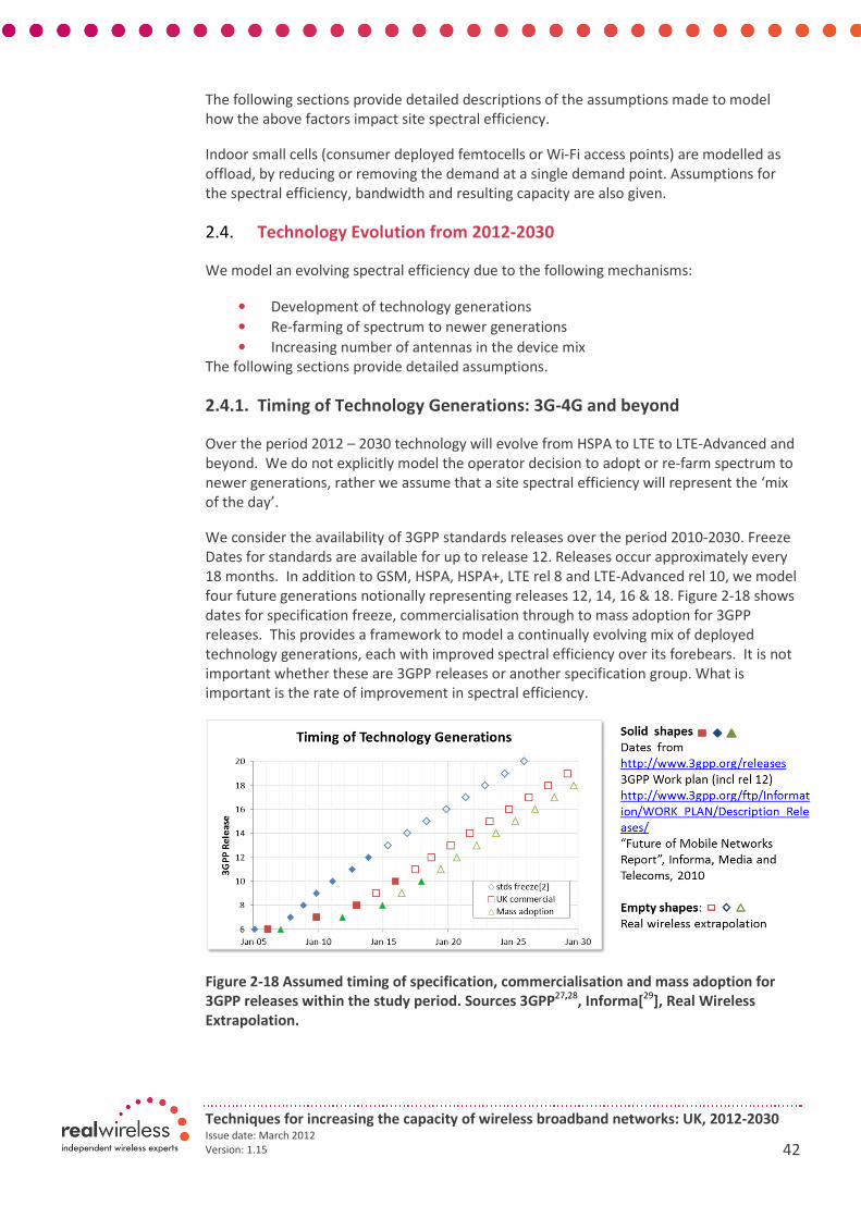
Techniques for increasing the capacity of wireless broadband networks: UK, 2012-2030 Issue date: March 2012
Version: 1.15 42
The following sections provide detailed descriptions of the assumptions made to model
how the above factors impact site spectral efficiency.
Indoor small cells (consumer deployed femtocells or Wi-Fi access points) are modelled as
offload, by reducing or removing the demand at a single demand point. Assumptions for
the spectral efficiency, bandwidth and resulting capacity are also given.
2.4. Technology Evolution from 2012-2030
We model an evolving spectral efficiency due to the following mechanisms:
• Development of technology generations
• Re-farming of spectrum to newer generations
• Increasing number of antennas in the device mix
The following sections provide detailed assumptions.
2.4.1. Timing of Technology Generations: 3G-4G and beyond
Over the period 2012 – 2030 technology will evolve from HSPA to LTE to LTE-Advanced and
beyond. We do not explicitly model the operator decision to adopt or re-farm spectrum to
newer generations, rather we assume that a site spectral efficiency will represent the ‘mix
of the day’.
We consider the availability of 3GPP standards releases over the period 2010-2030. Freeze
Dates for standards are available for up to release 12. Releases occur approximately every
18 months. In addition to GSM, HSPA, HSPA+, LTE rel 8 and LTE-Advanced rel 10, we model
four future generations notionally representing releases 12, 14, 16 & 18. Figure 2-18 shows
dates for specification freeze, commercialisation through to mass adoption for 3GPP
releases. This provides a framework to model a continually evolving mix of deployed
technology generations, each with improved spectral efficiency over its forebears. It is not
important whether these are 3GPP releases or another specification group. What is
important is the rate of improvement in spectral efficiency.
Figure 2-18 Assumed timing of specification, commercialisation and mass adoption for
3GPP releases within the study period. Sources 3GPP27,28
, Informa[29
], Real Wireless
Extrapolation.

Techniques for increasing the capacity of wireless broadband networks: UK, 2012-2030 Issue date: March 2012
Version: 1.15 43
2.4.2. Spectrum Usage per Technology Generation and Re-farming
Based on the findings of lead times from standards freeze to commercial availability and
mass adoption presented in our study of 4G Capacity Gains [30
], we model each technology
generation’s spectral occupancy building and falling over time as shown Figure 2-19. The
lower plot is a cumulative version of the upper plot, presenting the same information in a
different format. Generations beyond release 10 are assumed to follow similar trends to
earlier releases. GSM is treated a special case, and is gradually replaced or re-farmed over
time until 2020.
Spectral efficiency for a given year is computed as a sum of that of each generation,
weighted according the proportion of spectrum deployed with that generation. We note
that the total quantity of spectrum increases significantly during the study period, as
described in the section on spectrum scenarios.
Figure 2-19 Assumed evolution of spectrum usage by different technology generations
0%
10%
20%
30%
40%
50%
60%
70%
80%
20
10
20
15
20
20
20
25
20
30
% Spectrum Deployed per Tech Generation
GSM
HSPA R6
HSPA+
LTE r8
LTE-A r10
LTE-A r12
LTE-A r14
LTE-A r16
LTE-A r18
0%
20%
40%
60%
80%
100%
20
10
20
11
20
12
20
13
20
14
20
15
20
16
20
17
20
18
20
19
20
20
20
21
20
22
20
23
20
24
20
25
20
26
20
27
20
28
20
29
20
30
% Spectrum Deployed per Tech Generation
LTE-A r18
LTE-A r16
LTE-A r14
LTE-A r12
LTE-A r10
LTE r8
HSPA+
HSPA R6
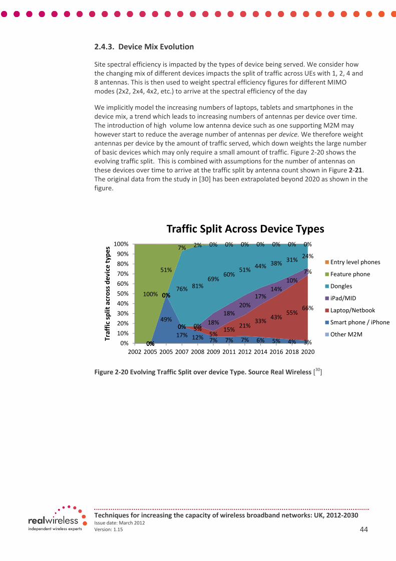
Techniques for increasing the capacity of wireless broadband networks: UK, 2012-2030 Issue date: March 2012
Version: 1.15 44
2.4.3. Device Mix Evolution
Site spectral efficiency is impacted by the types of device being served. We consider how
the changing mix of different devices impacts the split of traffic across UEs with 1, 2, 4 and
8 antennas. This is then used to weight spectral efficiency figures for different MIMO
modes (2x2, 2x4, 4x2, etc.) to arrive at the spectral efficiency of the day
We implicitly model the increasing numbers of laptops, tablets and smartphones in the
device mix, a trend which leads to increasing numbers of antennas per device over time.
The introduction of high volume low antenna device such as one supporting M2M may
however start to reduce the average number of antennas per device. We therefore weight
antennas per device by the amount of traffic served, which down weights the large number
of basic devices which may only require a small amount of traffic. Figure 2-20 shows the
evolving traffic split. This is combined with assumptions for the number of antennas on
these devices over time to arrive at the traffic split by antenna count shown in Figure 2-21.
The original data from the study in [30] has been extrapolated beyond 2020 as shown in the
figure.
Figure 2-20 Evolving Traffic Split over device Type. Source Real Wireless [30
]
0%
49%
17% 12% 7% 7% 7% 6% 5% 4% 3%0%
0%
0% 5%5%
15%21%
33%43%
55%66%
0%
0%
0% 0%18%
18%
20%
17%14%
10%
7%
0%
0%76% 81%
69%60%
51%44% 38%
31%24%
100%
51%
7% 2% 0% 0% 0% 0% 0% 0% 0%
0%
10%
20%
30%
40%
50%
60%
70%
80%
90%
100%
2002 2005 2005 2007 2008 2009 2011 2012 2014 2016 2018 2020
Tra
ffic
sp
lit
acr
oss
de
vic
e t
yp
es
Traffic Split Across Device Types
Entry level phones
Feature phone
Dongles
iPad/MID
Laptop/Netbook
Smart phone / iPhone
Other M2M
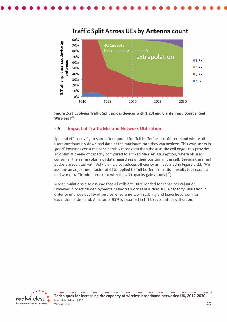
Techniques for increasing the capacity of wireless broadband networks: UK, 2012-2030 Issue date: March 2012
Version: 1.15 45
Figure 2-21 Evolving Traffic Split across devices with 1,2,4 and 8 antennas. Source Real
Wireless [30
]
2.5. Impact of Traffic Mix and Network Utilisation
Spectral efficiency figures are often quoted for ‘full buffer’ user traffic demand where all
users continuously download data at the maximum rate they can achieve. This way, users in
‘good’ locations consume considerably more data than those at the cell edge. This provides
an optimistic view of capacity compared to a ‘fixed file size’ assumption, where all users
consumer the same volume of data regardless of their position in the cell. Serving the small
packets associated with VoIP traffic also reduces efficiency as illustrated in Figure 2-22. We
assume an adjustment factor of 65% applied to ‘full buffer’ simulation results to account a
real world traffic mix, consistent with the 4G capacity gains study [30
].
Most simulations also assume that all cells are 100% loaded for capacity evaluation.
However in practical deployments networks work at less than 100% capacity utilisation in
order to improve quality of service, ensure network stability and leave headroom for
expansion of demand. A factor of 85% is assumed in [30
] to account for utilisation.

Techniques for increasing the capacity of wireless broadband networks: UK, 2012-2030 Issue date: March 2012
Version: 1.15 46
Figure 2-22 Impact of Traffic Type on Cell Spectral Efficiency, Source Real Wireless [30
]
2.6. Technology Evolution Scenarios Low, Mid, High:
In order to represent a range of possible evolution scenarios for standardised mobile
broadband technology, we consider three possibilities (low, mid, high).
• Little further growth (low): This assumes that the current day mobile broadband
technology is already approaching the limits of what is achievable in terms of site
spectral efficiency. It assumes that no significant benefits will be achieved in
practice with advanced techniques such as CoMP or enhanced MIMO due to
limitations of backhaul quality or space for more MIMO antennas
• Steady Growth (mid): The mid scenario represents a steady improvement in site
spectral efficiency, as algorithms improve and new techniques are introduced to
co-ordinate and reduce the interference which ultimately limits cell throughput.
Furthermore, we can assume Self Optimising Network technology automatically
adapts network configurations to optimally match the changing conditions in
which they operate.
• Innovation dividend (high): This ‘high’ scenario represents continued strong
growth in the spectral efficiency of mobile broadband technologies. Although we
cannot specify exactly how this will come about, the actual efficiency figures will
be based on a significant improvement over the ‘steady growth case’
The purpose of the scenarios is to model a spread of technology improvement which can
help us understand the sensitivity of our findings to our assumptions in this area. This also
enables us to ‘bound’ the plausible rates of technology improvement.
The scenarios impact the choice of spectral efficiency figures and growth beyond release 10
(LTE-Advanced) for which industry wide simulation results are available.
Techniques for increasing the capacity of wireless broadband networks: UK, 2012-2030 Issue date: March 2012
Version: 1.15 47
2.7. Cell Spectral Efficiency Per Generation, Per Antenna Configuration
2.7.1. GSM and HSPA
Assumptions for GSM and HSPA(+) technologies are based on the extensive analysis of 4G
capacity gains which provides figures for low, mid and high end deployments, shown in
Figure 2-23. The low, mid, high scenarios all start off the same in 2012, but diverge for later
years.
GSM is assumed to have a spectral efficiency of 0.09 bps/Hz/cell for all antenna
configurations, consistent with the 4G capacity gains report [30] and a previous PA
Consulting study [31
].
HSPA release 6 and 7 are based on [30
], which gives figures for low-end, med and high-end
device modems as shown in Figure 2-23. These device types are mapped onto this study’s
technology evolution scenarios as follows:
• HSPA Rel 6:
• Low scenario: low end, no evolution
• Mid scenario: Low end evolving to mid
• High scenario: low evolving to mid and high
• HSPA Rel 7:
• Low scenario: mid, no evolution
• Mid & High scenario: mid evolving to high end
‘Evolution’ is achieved by using the device antenna mix mechanism, where the device mix
starts with predominantly 1 and 2 antenna devices with increasingly more 4 and 8 antenna
devices. In the case of HSPA where 4 and 8 layer MIMO are not supported, these are
replaced with mid and the high-end device types.

Techniques for increasing the capacity of wireless broadband networks: UK, 2012-2030 Issue date: March 2012
Version: 1.15 48
Figure 2-23 Cell Spectral Efficiency figures used for GSM and HSPA release 6 and 7, Source
Real Wireless [30
]
2.7.2. LTE Release 8 and LTE-Advanced Release 10
The source data for LTE and LTE-Advanced are the industry-wide evaluations performed by
the 3GPP for their application of LTE-Advanced as an IMT-Advanced technology [32, 33
].
These sources provide a wide range of comparable results for LTE release 8 and 10 with
different antenna configurations algorithms and CoMP schemes and in both ‘3GPP case 1’
macrocell conditions and ITU-R ‘Urban Macrocell’ environment with a 2GHz carrier
frequency, described in detail in [34
]. In general the Urban Macrocell environment results
are used, but where results are missing, relationships between comparable results from
3GPP case 1 are scaled to the ITU environment. These results are applicable to an urban
macrocell with outdoor only demand at a mid carrier frequency. We show later how these
results are scaled to other environments.
These 3GPP simulation results represent ‘full buffer’ traffic models and 100% network
utilisation. They are scaled according to a ‘real world’ traffic mix and utilisation given
earlier. This is broadly the approach used by the 4G capacity gains study30 and was found
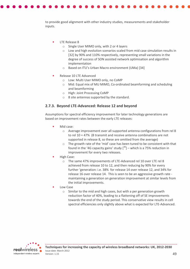
Techniques for increasing the capacity of wireless broadband networks: UK, 2012-2030 Issue date: March 2012
Version: 1.15 49
to provide good alignment with other industry studies, measurements and stakeholder
inputs.
• LTE Release 8
o Single User MIMO only, with 2 or 4 layers
o Low and high evolution scenarios scaled from mid case simulation results in
[32] by 90% and 110% respectively, representing small variations in the
degree of success of SON assisted network optimisation and algorithm
implementation
o Based on ITU’s Urban Macro environment (UMa) [34]
• Release 10 LTE Advanced
o Low: Multi User MIMO only, no CoMP
o Mid: Equal mix of MU MIMO, Co-ordinated beamforming and scheduling
and beamforming
o High: Joint Processing CoMP
o 8 site antennas supported by the standard.
2.7.3. Beyond LTE-Advanced: Release 12 and beyond
Assumptions for spectral efficiency improvement for later technology generations are
based on improvement rates between the early LTE releases:
• Mid case:
o Average improvement over all supported antenna configurations from rel 8
to rel 10 = 47% (8 transmit and receive antenna combinations are not
supported in release 8, so these are omitted from the average)
o The growth rate of the ‘mid’ case has been tuned to be consistent with that
found in the ‘4G capacity gains’ study [30
] – which is a 75% reduction in
improvement for every two releases.
• High Case:
o The same 47% improvements of LTE-Advanced rel 10 over LTE rel 8
achieved from release 10 to 12, and then reducing by 90% for every
further ‘generation: i.e. 38% for release 14 over release 12, and 34% for
release 16 over release 14. This is seen to be an aggressive growth rate -
maintaining a generation on generation improvement at similar levels from
the initial improvements.
• Low Case
o Similar to the mid and high cases, but with a per generation growth
reduction factor of 40%, leading to a flattening off of SE improvements
towards the end of the study period. This conservative view results in cell
spectral efficiencies only slightly above what is expected for LTE-Advanced.
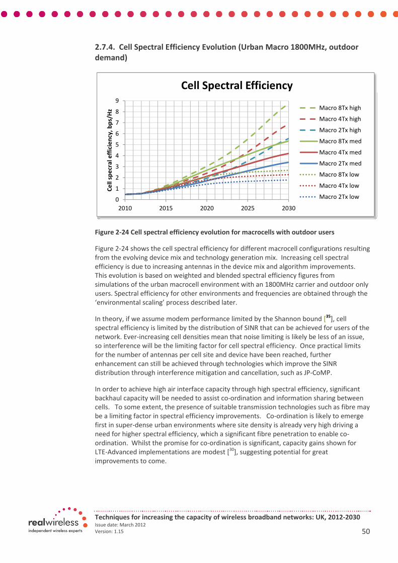
Techniques for increasing the capacity of wireless broadband networks: UK, 2012-2030 Issue date: March 2012
Version: 1.15 50
2.7.4. Cell Spectral Efficiency Evolution (Urban Macro 1800MHz, outdoor
demand)
Figure 2-24 Cell spectral efficiency evolution for macrocells with outdoor users
Figure 2-24 shows the cell spectral efficiency for different macrocell configurations resulting
from the evolving device mix and technology generation mix. Increasing cell spectral
efficiency is due to increasing antennas in the device mix and algorithm improvements.
This evolution is based on weighted and blended spectral efficiency figures from
simulations of the urban macrocell environment with an 1800MHz carrier and outdoor only
users. Spectral efficiency for other environments and frequencies are obtained through the
‘environmental scaling’ process described later.
In theory, if we assume modem performance limited by the Shannon bound [35
], cell
spectral efficiency is limited by the distribution of SINR that can be achieved for users of the
network. Ever-increasing cell densities mean that noise limiting is likely be less of an issue,
so interference will be the limiting factor for cell spectral efficiency. Once practical limits
for the number of antennas per cell site and device have been reached, further
enhancement can still be achieved through technologies which improve the SINR
distribution through interference mitigation and cancellation, such as JP-CoMP.
In order to achieve high air interface capacity through high spectral efficiency, significant
backhaul capacity will be needed to assist co-ordination and information sharing between
cells. To some extent, the presence of suitable transmission technologies such as fibre may
be a limiting factor in spectral efficiency improvements. Co-ordination is likely to emerge
first in super-dense urban environments where site density is already very high driving a
need for higher spectral efficiency, which a significant fibre penetration to enable co-
ordination. Whilst the promise for co-ordination is significant, capacity gains shown for
LTE-Advanced implementations are modest [30
], suggesting potential for great
improvements to come.
0
1
2
3
4
5
6
7
8
9
2010 2015 2020 2025 2030
Ce
ll s
pe
cra
l e
ffic
ien
cy,
bp
s/H
z
Cell Spectral Efficiency
Macro 8Tx high
Macro 4Tx high
Macro 2Tx high
Macro 8Tx med
Macro 4Tx med
Macro 2Tx med
Macro 8Tx low
Macro 4Tx low
Macro 2Tx low

Techniques for increasing the capacity of wireless broadband networks: UK, 2012-2030 Issue date: March 2012
Version: 1.15 51
2.8. Sectorisation Gains
Cell spectral efficiencies are converted to site spectral efficiencies through multiplication by
the sectorisation gain.
Figure 2-25 Sectorisation Gains for Different Sector Antenna Beamwidths, Source Jaiho et
al[36
]
Each sector antenna provides a ‘cell’ of coverage in which the spectral resource is re-used.
More sectors means higher site spectral efficiency. There are diminishing returns for
sectorisation gain where pattern roll-off causes adjacent sector interference. Larger
apertures are needed for the tighter roll-off needed for higher order sectorisation. Softer
handoff in 3G can exploit adjacent sector interference to increase site capacity. Although
early HSPA and LTE only support hard handover, techniques like intra-site CoMP work in
much the same way as soft(er) handoff. Scattering around the site can also increase
adjacent sector interference- an issue for microcells in the clutter. The operators’ choice
between 3 and 6 sector macro sites (combined with 2,4,8 Tx antennas) is explicitly
modelled.
Source data for macro site cell spectral efficiency is based on trisector sites, so a straight
forward multiple of 3x is needed here. For 6 sector sites, a sectorisation gain of 5.6x is used
based on [36
] (see above graph, assuming the 33 degree antenna.
Initially outdoor small cell sites are assumed to have a single sector, with 2 sector small cell
sites increasing in the mix towards 2030 (details are provided later).

Techniques for increasing the capacity of wireless broadband networks: UK, 2012-2030 Issue date: March 2012
Version: 1.15 52
2.9. Adjustments for Outdoor Small Cells
Operators are now looking to deploy small cell technology themselves to meet capacity
needs in hot spot areas, where there is no remaining places for macrosites. It is anticipated
that site acquisition can be simplified through single landlord deals such as on authority
managed street furniture, or shop facades for chain stores. Benefits over femtocells are
managed deployment and backhaul leading to improved QoS, including handover, latency
and throughput.
Spectral efficiency for small cells is based on a blend of macrocell spectral efficiency for 2
and 4 tx antennas and 1 and two sectors, scaled to represent the increase from the
environment.
Small cells have smaller form factors to enable them to be deployed in wider variety of
locations than macro-sites, which typically require space for outdoor and indoor
equipment. The smaller size does limit the RF power and hence range that small cells
provide, so they needed to be deployed close to the users, down at street level.
Deployment ‘down in the clutter’ results in a different propagation environment to rooftop
macrocells, and it is believed the resulting isolation between cells reduces interference and
results in higher spectral efficiency, as summarised in Table 7. The 3GPP and Deutsche
Telekom sources are the most credible here, since they are based on an analysis of the
small cell environment. The ITU-R is a requirement rather than the result of analysis, and so
is indicative of an expectation that small cell spectral efficiency should be higher. Picochip
and Huawei sources made no allowance for any difference between macro and small cell
efficiency, and these are more likely to be the result of simplification rather than a
considered analysis. We believe a scaling figure of 1.24 represents the most credible of
these sources.
Source Scaling factor: SEsmallcell: SEmacro (DL)
3GPP simulations33
1.24x
Deutsche Telekom37
1.25x (0.5-2x)
ITU-R38
(requirements) 1.18x
Picochip39
~1x but inconclusive
Huawei (2 sources)40, 41
1x assumed
Proposed scaling factor: 1.24x
Table 7 Scaling macrocell spectral efficiencies to small cells due to the different
propagation environment
Unlike macrosites, where sectorisation and number of transmit antennas will be explicitly
modelled as an upgrade option, it is assumed that small cells will be replaced rather than

Techniques for increasing the capacity of wireless broadband networks: UK, 2012-2030 Issue date: March 2012
Version: 1.15 53
upgraded, and that the site spectral efficiency will represent the ‘mix of the day’. We expect
to see an evolution of small cell technology from single sector only towards two sectors
(which may for example point in opposite directions down a street) and from 2 antennas to
4 antennas, enabling the higher order MIMO modes. Figure 2-26 shows the assumed mix
over the study period. By 2024 we expect all outdoor small cells to support 4 transmit
antenna MIMO. At the device end, we assume the same mix of 2,4 and 8 antenna devices
as used for macrocells.
Figure 2-26 Assumption for evolving mix of 2 and 4 transmit antenna outdoor small cells
Initially outdoor small cells are all single sector devices; however, we anticipate that 2
sector devices will be introduced, for example with different sectors in opposite directions
up and down a street. Figure 2-27 shows the assumed mix of 1 and 2 sector small cell sites.
By 2030 50% of small cell sites are assumed to support two cells per site.
Figure 2-27 Assumption for the evolving mix of small cells sites with 1 and 2 cells per site
0%
20%
40%
60%
80%
100%
2010 2012 2014 2016 2018 2020 2022 2024 2026 2028 2030
Evolving Transmit Antenna Mix
4 Antennas
2 Antennas
0%
20%
40%
60%
80%
100%
2010 2012 2014 2016 2018 2020 2022 2024 2026 2028 2030
Evolving Cells per site mix
2 cells / site
1 cell / site

Techniques for increasing the capacity of wireless broadband networks: UK, 2012-2030 Issue date: March 2012
Version: 1.15 54
2.10. Site Spectral Efficiency
Figure 2-28 Site spectral Efficiency Evolution for Mid Case Macro and Outdoor small cells
with outdoor consumers
Figure 2-28 shows site spectral efficiency resulting from the combination of cell spectral
efficiency with sectorisation gain, and in the case of outdoor small cells, the sectorisation
and transmit antenna mix. This represents spectral efficiency with outdoor only consumers
in an urban environment with an 1800MHz carrier frequency. Scaling factors applied to
represent other environments are described later. The slight undulations in the curves are
the result of moving between the technology generations, which is largely averaged out by
the overlap between generations shown earlier.
Figure 2-29 compares the low, mid and high technology evolution scenarios for an example
site configuration. Other configurations have broadly the same relationship. Spectral
efficiency for all scenarios is similar at the beginning of the study period, where we have a
confident view of what is achieved in practice today. The lines diverge in the latter part of
the study period as predictions are increasingly speculative. Relative to the mid case in
2030, the low and high cases are 54% lower and 64% higher respectively. The low to high
represents a range of 3.0x.
0
2
4
6
8
10
12
14
16
18
20
20
10
20
11
20
12
20
13
20
14
20
15
20
16
20
17
20
18
20
19
20
20
20
21
20
22
20
23
20
24
20
25
20
26
20
27
20
28
20
29
20
30
bp
s/H
z/si
te
Site Spectral Efficiency Evolution for Various Configurations
Mid - Steady Technology Improvement
Macro 6sec, 2tx
Macro 3sec, 8tx
Macro 3sec, 4tx
Macro 3sec, 2tx
Outdoor Sm Cell
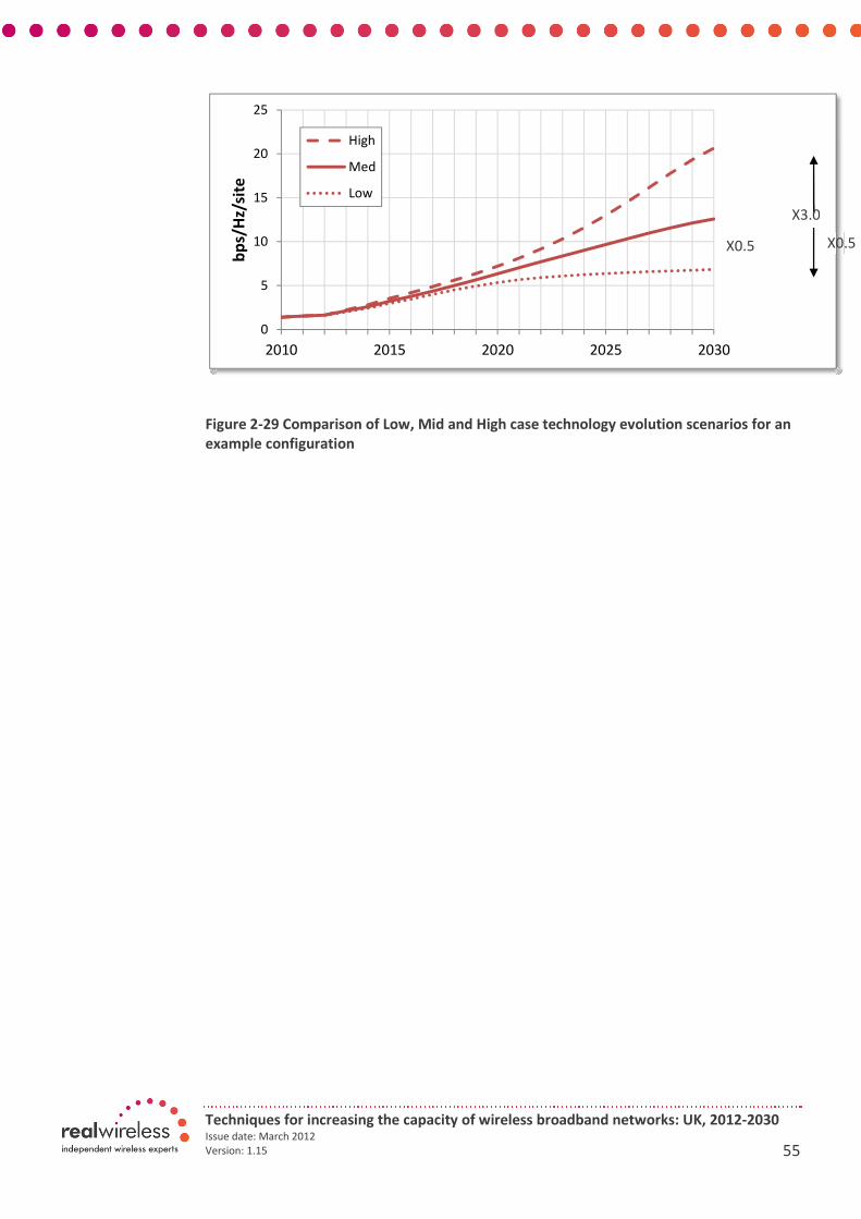
Techniques for increasing the capacity of wireless broadband networks: UK, 2012-2030 Issue date: March 2012
Version: 1.15 55
Figure 2-29 Comparison of Low, Mid and High case technology evolution scenarios for an
example configuration
0
5
10
15
20
25
2010 2015 2020 2025 2030
bp
s/H
z/si
te
High
Med
Low
X0.5
X3.0
X0.5

Techniques for increasing the capacity of wireless broadband networks: UK, 2012-2030 Issue date: March 2012
Version: 1.15 56
2.11. Environmental Scaling for Geotypes, Carrier Frequency and Indoor
Users
Site spectral efficiencies for outdoor only consumers are adjusted by a range of scaling
factors to represent indoor only users for different clutter types and carrier frequencies.
The model itself then combines the outdoor only and indoor only figures to represent the
actual mix.
Scaling factors are obtained from an analysis of SINR distributions generated by a model
designed for coverage and capacity analysis by Ofcom[42
]. This uses site and demand point
data as defined under study areas, which are based on site counts equivalent to 13k sites
UK wide. SINR CDFs are obtained for outdoor-only UEs and indoor-only UEs (10m depth
“Depth1+”). Indoor penetration losses vary with frequency consistent with the link budgets
used in this study for site range calculations. Figure 2-30 shows SINR distributions for the
rural Lincolnshire study area. Similar results were obtained for the other study areas.
Note that this SINR analysis is based on an 800MHz spot frequency, whereas our site ranges
assume 700MHz. In both cases we are applying the findings to represent all bands in the
<1GHz group, so it not critical that they are the same. We expect that any differences in the
performance at these spot frequencies can be assumed to be negligible.
Figure 2-30 Example SINR distributions from a coverage analysis, used to determine ratio
of spectral efficiency between outdoor and indoor
The resulting SINR distributions are combined with link level performance for 2x2, 4x2 and
4x4 configurations from a 3G Americas report [43
] to yield cell spectral efficiencies.
Differences in SE for 2x2, 2x4 and 4x4 MIMO antenna configurations were all less than
0.5%, so environmental scaling is considered to be independent of antenna configuration.
0%
10%
20%
30%
40%
50%
60%
70%
80%
90%
100%
-30 -25 -20 -15 -10 -5 0 5 10 15 20 25
CD
F
SINR, dB
SINR CDFs for Indoor and Outdoor Users, 3 frequencies
Rur Lincs Out 800
Rur Lincs Out 1800
Rur Lincs Out 2600
Rur Lincs In 800
Rur Lincs In 1800
Rur Lincs In 2600
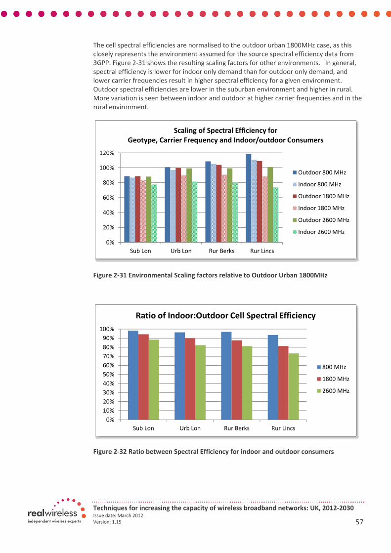
Techniques for increasing the capacity of wireless broadband networks: UK, 2012-2030 Issue date: March 2012
Version: 1.15 57
The cell spectral efficiencies are normalised to the outdoor urban 1800MHz case, as this
closely represents the environment assumed for the source spectral efficiency data from
3GPP. Figure 2-31 shows the resulting scaling factors for other environments. In general,
spectral efficiency is lower for indoor only demand than for outdoor only demand, and
lower carrier frequencies result in higher spectral efficiency for a given environment.
Outdoor spectral efficiencies are lower in the suburban environment and higher in rural.
More variation is seen between indoor and outdoor at higher carrier frequencies and in the
rural environment.
Figure 2-31 Environmental Scaling factors relative to Outdoor Urban 1800MHz
Figure 2-32 Ratio between Spectral Efficiency for indoor and outdoor consumers
0%
20%
40%
60%
80%
100%
120%
Sub Lon Urb Lon Rur Berks Rur Lincs
Scaling of Spectral Efficiency for
Geotype, Carrier Frequency and Indoor/outdoor Consumers
Outdoor 800 MHz
Indoor 800 MHz
Outdoor 1800 MHz
Indoor 1800 MHz
Outdoor 2600 MHz
Indoor 2600 MHz
0%
10%
20%
30%
40%
50%
60%
70%
80%
90%
100%
Sub Lon Urb Lon Rur Berks Rur Lincs
Ratio of Indoor:Outdoor Cell Spectral Efficiency
800 MHz
1800 MHz
2600 MHz
Techniques for increasing the capacity of wireless broadband networks: UK, 2012-2030 Issue date: March 2012
Version: 1.15 58
Figure 2-32 shows the indoor:outdoor ratio of cell spectral efficiencies at different carrier
frequencies for each study area. This reveals on of the key benefits of sub 1GHz spectrum –
that it can serve indoor users with high spectral efficiency even in rural environments. Using
higher carrier frequencies for indoor coverage results in moderate reductions of cell
spectral efficiency (almost 30% for 2600MHz in the Rural Lincolnshire study area).
Note that this may appear to contradict some views that lower frequencies are poor for
capacity and are better suited for coverage applications. These views arise from two
sources:
1. The quantity of spectrum available in lower frequency bands is usually more limited;
2. That the lower propagation losses at lower frequencies may cause excessive interference between sites in high capacity density areas.
Our modelling explicitly incorporates the available spectrum quantities at each band,
addressing (1) above. Regarding (2), while indeed frequency reuse requires greater care in
order to contain interference at lower frequencies, this can be achieved via a variety of
techniques including antenna tilts, beamforming, power control and smart scheduling.
Once these are included, the improved propagation is an advantage for spectrum
efficiency, as demonstrated in the modelling results above.
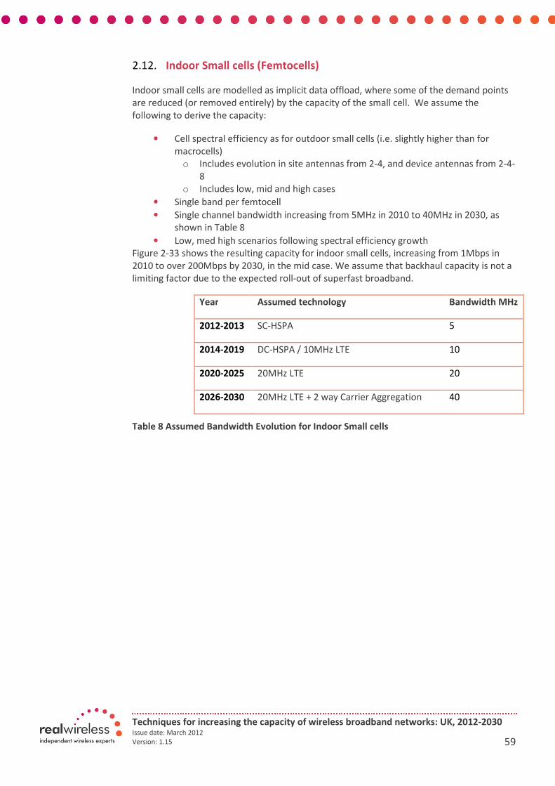
Techniques for increasing the capacity of wireless broadband networks: UK, 2012-2030 Issue date: March 2012
Version: 1.15 59
2.12. Indoor Small cells (Femtocells)
Indoor small cells are modelled as implicit data offload, where some of the demand points
are reduced (or removed entirely) by the capacity of the small cell. We assume the
following to derive the capacity:
• Cell spectral efficiency as for outdoor small cells (i.e. slightly higher than for
macrocells)
o Includes evolution in site antennas from 2-4, and device antennas from 2-4-
8
o Includes low, mid and high cases
• Single band per femtocell
• Single channel bandwidth increasing from 5MHz in 2010 to 40MHz in 2030, as
shown in Table 8
• Low, med high scenarios following spectral efficiency growth
Figure 2-33 shows the resulting capacity for indoor small cells, increasing from 1Mbps in
2010 to over 200Mbps by 2030, in the mid case. We assume that backhaul capacity is not a
limiting factor due to the expected roll-out of superfast broadband.
Year Assumed technology Bandwidth MHz
2012-2013 SC-HSPA 5
2014-2019 DC-HSPA / 10MHz LTE 10
2020-2025 20MHz LTE 20
2026-2030 20MHz LTE + 2 way Carrier Aggregation 40
Table 8 Assumed Bandwidth Evolution for Indoor Small cells

Techniques for increasing the capacity of wireless broadband networks: UK, 2012-2030 Issue date: March 2012
Version: 1.15 60
Figure 2-33 Indoor Small Cell Capacity Evolution over the Study Period
1
10
100
1000
20
10
20
11
20
12
20
13
20
14
20
15
20
16
20
17
20
18
20
19
20
20
20
21
20
22
20
23
20
24
20
25
20
26
20
27
20
28
20
29
20
30
Mb
ps
pe
r S
ma
ll C
ell
Site Capacity For Indoor Small Cell
High
Mid
Low

Techniques for increasing the capacity of wireless broadband networks: UK, 2012-2030 Issue date: March 2012
Version: 1.15 61
A3. Spectrum scenarios
3.1. Introduction
This annex explains the sources of the spectrum scenarios used in our modelling, which
have been developed in close discussion with Ofcom.
We considered individual mobile spectrum bands that could become available for use in the
UK based on a set of selection criteria. The criteria helped to identify those spectrum bands
that are available today or could become available in the future for mobile use. The criteria
used to select the spectrum bands are given below:
• Will the spectrum be allocated for mobile / harmonised use?
• Will the band be cleared/available for use in the UK?
• Will the band be used at scale (standardised) internationally
• Will the band be attractive (i.e. given factors like adjacent use interference etc.)?
If a band is selected, then the relevant quantity is determined by considering the following:
• How much spectrum is there in the band?
• Are there adjustments to make to the amount that is actually available (e.g.
guard bands etc.)?
• Is there sufficient to be attractive for deployment in practice
The format for modelling the spectrum input required the net spectrum bandwidth for the
downlink portion only since the study was interested in delivering capacity to users, as this
is limiting factor within current mobile broadband networks. It is accepted that the
symmetry of networks may shift over time but we assume the majority of traffic provision
and associated limits on capacity will be predominantly in the downlink (Note however that
in some cases the uplink may limit range and we have incorporated this in our site range
calculations). Furthermore, the spectrum was to be available across the UK in the time
frame between 2012 and 2030.
Paired and unpaired spectrum were both under consideration and we factored in the
proportion of time that TDD systems allocate to the downlink.
The gross spectrum quantities were identified to give the total spectrum for each band.
However, in order to determine the precise amount of net spectrum available for use in the
model we had to take into account various factors such as future availability, re-farming
etc. Other specific considerations for deriving net spectrum also included the use of guard
bands, duplex spacing etc.
The assumptions we made to determine the quantity and timing of introducing each of the
frequency bands were based on the best available information and confirmatory
discussions with Ofcom. The current status of spectrum bands in the UK was derived
according to the Frequency Allocations Table[44
] and the UK Interface Requirements (See
Table 12, Table 13 and Table 15 for specific reference) , or from public sector spectrum
announcements for the release of MOD spectrum or other public sector spectrum under
the spectrum release programme[45
].
We identified 17 (2 in the high case only) distinct frequency bands that will be made
available for capacity purposes over the whole timeframe. The quantity and timing of each
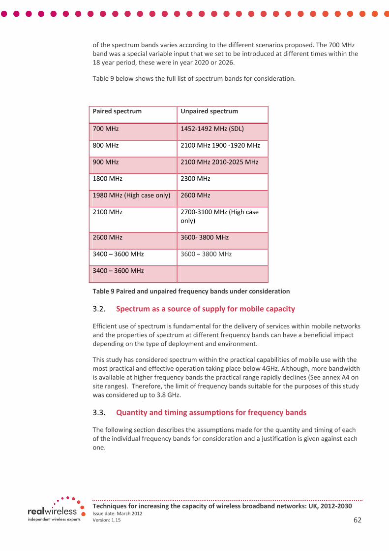
Techniques for increasing the capacity of wireless broadband networks: UK, 2012-2030 Issue date: March 2012
Version: 1.15 62
of the spectrum bands varies according to the different scenarios proposed. The 700 MHz
band was a special variable input that we set to be introduced at different times within the
18 year period, these were in year 2020 or 2026.
Table 9 below shows the full list of spectrum bands for consideration.
Paired spectrum Unpaired spectrum
700 MHz 1452-1492 MHz (SDL)
800 MHz 2100 MHz 1900 -1920 MHz
900 MHz 2100 MHz 2010-2025 MHz
1800 MHz 2300 MHz
1980 MHz (High case only) 2600 MHz
2100 MHz 2700-3100 MHz (High case
only)
2600 MHz 3600- 3800 MHz
3400 – 3600 MHz 3600 – 3800 MHz
3400 – 3600 MHz
Table 9 Paired and unpaired frequency bands under consideration
3.2. Spectrum as a source of supply for mobile capacity
Efficient use of spectrum is fundamental for the delivery of services within mobile networks
and the properties of spectrum at different frequency bands can have a beneficial impact
depending on the type of deployment and environment.
This study has considered spectrum within the practical capabilities of mobile use with the
most practical and effective operation taking place below 4GHz. Although, more bandwidth
is available at higher frequency bands the practical range rapidly declines (See annex A4 on
site ranges). Therefore, the limit of frequency bands suitable for the purposes of this study
was considered up to 3.8 GHz.
3.3. Quantity and timing assumptions for frequency bands
The following section describes the assumptions made for the quantity and timing of each
of the individual frequency bands for consideration and a justification is given against each
one.
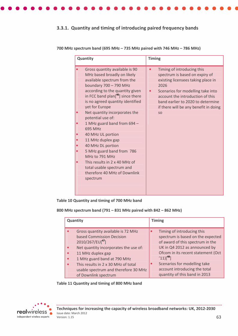
Techniques for increasing the capacity of wireless broadband networks: UK, 2012-2030 Issue date: March 2012
Version: 1.15 63
3.3.1. Quantity and timing of introducing paired frequency bands
700 MHz spectrum band (695 MHz – 735 MHz paired with 746 MHz – 786 MHz)
Quantity Timing
• Gross quantity available is 90
MHz based broadly on likely
available spectrum from the
boundary 700 – 790 MHz
according to the quantity given
in FCC band plan[46
] since there
is no agreed quantity identified
yet for Europe
• Net quantity incorporates the
potential use of:
• 1 MHz guard band from 694 –
695 MHz
• 40 MHz UL portion
• 11 MHz duplex gap
• 40 MHz DL portion
• 5 MHz guard band from 786
MHz to 791 MHz
• This results in 2 x 40 MHz of
total usable spectrum and
therefore 40 MHz of Downlink
spectrum
• Timing of introducing this
spectrum is based on expiry of
existing licensees taking place in
2026
• Scenarios for modelling take into
account the introduction of this
band earlier to 2020 to determine
if there will be any benefit in doing
so
Table 10 Quantity and timing of 700 MHz band
800 MHz spectrum band (791 – 831 MHz paired with 842 – 862 MHz)
Quantity Timing
• Gross quantity available is 72 MHz
based Commission Decision
2010/267/EU[47
]
• Net quantity incorporates the use of:
• 11 MHz duplex gap
• 1 MHz guard band at 790 MHz
• This results in 2 x 30 MHz of total
usable spectrum and therefore 30 MHz
of Downlink spectrum
• Timing of introducing this
spectrum is based on the expected
of award of this spectrum in the
UK in Q4 2012 as announced by
Ofcom in its recent statement (Oct
’11)[48
]
• Scenarios for modelling take
account introducing the total
quantity of this band in 2013
Table 11 Quantity and timing of 800 MHz band

Techniques for increasing the capacity of wireless broadband networks: UK, 2012-2030 Issue date: March 2012
Version: 1.15 64
900 MHz frequency band (880 MHz – 915 MHz paired with 925 MHz – 960 MHz)
Quantity Timing
• Gross quantity available is 70
MHz based on Ofcom Interface
Requirement IR 2014 Public
Wireless[49
] Networks (Aug
2005)
• Net quantity is equal to gross
quantity with all duplex gaps
and guard bands already taken
into account with 2 x 35 MHz
available in total
• This results in 35 MHz of
Downlink spectrum
• This band is already available for
HSPA with at least one 5 MHz
carrier used in London by O2
• We assume HSPA is being used
today (2011) 5 MHz carrier used
for London for mobile broadband
and increases to 10 MHz in 2013
through to 2016, then increases
linearly to 35 MHz to 2021. This is
based on the majority of the
spectrum still being used for GSM
across the period
• After this point (2021) the band is
assumed to be fully refarmed
• This assumption is supported by
the increasing availability of HSPA
devices at 900 MHz according to
the Global Mobile Suppliers
Association[50
]
Table 12 Quantity and timing of 900 MHz band
1800 MHz frequency band (1710 MHz – 1785 MHz paired with 1805 MHz – 1880 MHz)
Quantity Timing
• Gross quantity available is 150
MHz based Interface
Requirement IR2014[49
] Public
Wireless Networks (Aug 2005)
• Net quantity will be 144 MHz
including the 2 x 15 MHz
released to the market. All
duplex gaps and guard bands
already taken into account
with 2 x 72 MHz available in
total
• This results in 72 MHz of
Downlink spectrum
• This band is currently (2011) used
for GSM.
• The 1800 MHz band is liberalised
for HSPA (2013). We have assumed
therefore only 22 MHz available
(DL) for HSPA/LTE over a 3 year
period to 2016. This is based on the
majority of the spectrum still being
used for GSM
• After this point (2016) the quantity
linearly increases over a five year
period until it fully refarmed by
2020.
• This assumption is supported by the
increasing availability of devices at
1800 MHz predominantly for LTE
according to the GSA[51
]
Table 13 Quantity and timing of 1800 MHz band

Techniques for increasing the capacity of wireless broadband networks: UK, 2012-2030 Issue date: March 2012
Version: 1.15 65
1980 MHz (High case only) frequency band (Frequency separation not yet defined for
terrestrial mobile use)
Quantity Timing
• Gross quantity available is 60
MHz based on globally
harmonised allocation[44
] for
Mobile satellite. The band is
adjacent to the IMT bands
• Net quantity assumes the use of
similar guard bands and duplex
gaps currently in place resulting
in 2 x 30 MHz available in total
• This results in 30 MHz of
Downlink spectrum
• This band is currently used for Mobile
satellite use and is only considered in
the high spectrum case scenario. MSS
is likely to remain until re-allocation
takes place no earlier than 2020
• We assume full availability of the
band from 2020 onwards for mobile
broadband services
Table 14 Quantity and timing of 1980 MHz band
2100 MHz frequency band (1920 MHz – 1980 MHz paired with 2110 MHz – 2170 MHz)
Quantity Timing
• Gross quantity available is 120
MHz based on IR 2019 Third
Generation Mobile[52
]
• Net quantity incorporates the use
of guard bands and duplex gaps
resulting in 2 x 60 MHz available in
total
• This results in 60 MHz of Downlink
spectrum
• This band is currently used for HSPA
and likely to continue to be used
predominantly for evolutions of HSPA
up to 2020
• We assume full use of the band from
2010 onwards for mobile broadband
services
Table 15 Quantity and timing of 2100 MHz band

Techniques for increasing the capacity of wireless broadband networks: UK, 2012-2030 Issue date: March 2012
Version: 1.15 66
2600 MHz frequency band (2500 MHz – 2570 MHz paired with 2620 MHz – 2690 MHz)
Quantity Timing
• Gross quantity available is 140 MHz
based on ECC Decision (05)05[53
]
• Net quantity includes a total of 2 x 70
MHz of usable spectrum which takes
into account duplex gap and guard
bands
• This results in 70 MHz of Downlink
spectrum
• Timing of introducing this
spectrum is based on the
expected of award of this
spectrum in the UK in Q4 2012 as
announced by Ofcom in its
recent statement[48
] (Oct ’11)
• Scenarios for modelling take
account introducing this band in
2013
Table 16 Quantity and timing of 2600 MHz band

Techniques for increasing the capacity of wireless broadband networks: UK, 2012-2030 Issue date: March 2012
Version: 1.15 67
3500 MHz frequency band (3480 – 3500 MHz paired with 3580 – 3600 MHz UK Broadband
spectrum and 3410 MHz – 3480 MHz paired with 3510 MHz – 3580 MHz)
Quantity Timing
• 3480 – 3500 MHz paired with
3580 – 3600 MHz Gross
quantity available is 40 MHz
based on Interface
Requirement IR2015[54
] (2011)
noting amendment of licence
to mobile
• Net quantity will be 20 MHz
based on 3GPP 36.101[55
]
Release 10 September 2011
resulting in 2 x 10 MHz and
therefore 10 MHz of Downlink
spectrum
• This band is currently used by UK
Broadband for mobile Wireless
Broadband services
• We assume this band will be used
for a future LTE network which is
likely to be available as early as
2012 as announced by UK
Broadband[56
]
• 3410 MHz – 3480 MHz paired
with 3510 MHz – 3580 MHz
• Gross quantity available is 140
MHz (excl UKB spectrum) as
stated in DCMS Enabling UK
growth – Releasing public
spectrum Making 500 MHz of
spectrum available by 2020[45]
• Net quantity will be 140 MHz (2 x
70 MHz) based on 3GPP 36.101
Release 10 September 2011[55]
which identifies 2 x 80 MHz in
this whole spectrum band. This
also assumes partial release to
market and the need for the
MOD to retain spectrum for
defence purposes
• This results in 70 MHz of
Downlink spectrum
• This band is currently used for
defence purposes but is a high
priority for release by the MOD
under its release programme
• The DCMS reports that the release
of this spectrum is likely to be
within current Government
spending round i.e. March 2015
• We have assumed some
approximate quantities to be made
available over the time frame:
• Less than 1/3 of this spectrum to
be made available in the low
quantity scenario over the whole
time frame
• ½ of the spectrum to be made
available in the baseline case up to
2025 from 2026 all spectrum is
made available
• Over 2/3 of this spectrum will be
made available in the high quantity
scenario over first five years of
release from 2016 to 2020 and from
2021 all spectrum is made available
• This is due to the various licensing
and sharing arrangements likely to
be put in place by the MOD
resulting in a phased approach to
release.
Table 17 Quantity and timing of 3500 MHz band

Techniques for increasing the capacity of wireless broadband networks: UK, 2012-2030 Issue date: March 2012
Version: 1.15 68
3.3.2. Quantity and timing of introducing unpaired frequency bands
The downlink portion for TDD systems differs to that of FDD due to sharing of spectrum
resources between the uplink and downlink. Therefore, we have assumed a proportion of
traffic generated by the downlink based on a set of TD-LTE frame configurations developed
by 3GPP57. The chart in Figure 3-1 shows the ranges of percentage of DL for TD-LTE and we
have assumed 89% in the downlink based on the majority of time spent in the downlink to
support growing demands for mobile traffic. All downlink spectrum in the following tables
have been adjusted by 89% from the total net quantity.
Figure 3-1 TD-LTE frame configurations and % resource allocated to DL. Source: 3GPP[57
]
1452 -1492 MHz frequency band
Quantity Timing
• Gross quantity available is 40
MHz based on ECC DEC 03(02)58
• Net quantity incorporates all 40
MHz use for TDD operation as a
supplemental downlink. Plum
conducted a study[59
] which
investigated the economic
benefits from use of 1452-1492
MHz for a supplemental mobile
downlink for enhanced
multimedia and broadband
services
• Timing of introducing this spectrum is
based on Plum’s report which takes
into account conclusion of ECC
decision end of 2012, inclusion of the
band by 3GPP and availability of
devices
• We assume the availability of all 40
MHz will be from 2014 to create a
supplemental downlink band for
mobile broadband use
Table 18 Quantity and timing of 1452 - 1492 MHz band
Uplink-
downlink%DL
configuration 0 1 2 3 4 5 6 7 8 9 U D
0 D S U U U D S U U U 6 2 25%
1 D S U U D D S U U D 4 4 50%
2 D S U D D D S U D D 2 6 75%
3 D S U U U D D D D D 3 6 67%
4 D S U U D D D D D D 2 7 78%
5 D S U D D D D D D D 1 8 89%
6 D S U U U D S U U D 5 3 38%
Subframe number totals
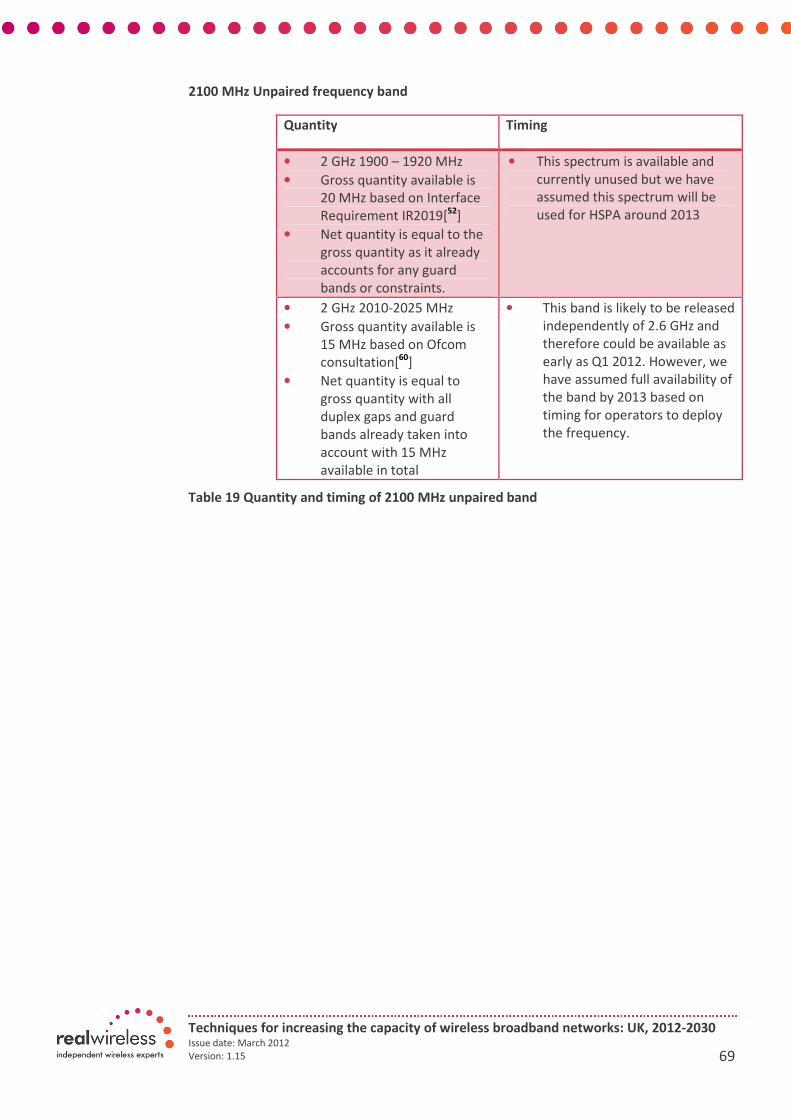
Techniques for increasing the capacity of wireless broadband networks: UK, 2012-2030 Issue date: March 2012
Version: 1.15 69
2100 MHz Unpaired frequency band
Quantity Timing
• 2 GHz 1900 – 1920 MHz
• Gross quantity available is
20 MHz based on Interface
Requirement IR2019[52
]
• Net quantity is equal to the
gross quantity as it already
accounts for any guard
bands or constraints.
• This spectrum is available and
currently unused but we have
assumed this spectrum will be
used for HSPA around 2013
• 2 GHz 2010-2025 MHz
• Gross quantity available is
15 MHz based on Ofcom
consultation[60
]
• Net quantity is equal to
gross quantity with all
duplex gaps and guard
bands already taken into
account with 15 MHz
available in total
• This band is likely to be released
independently of 2.6 GHz and
therefore could be available as
early as Q1 2012. However, we
have assumed full availability of
the band by 2013 based on
timing for operators to deploy
the frequency.
Table 19 Quantity and timing of 2100 MHz unpaired band
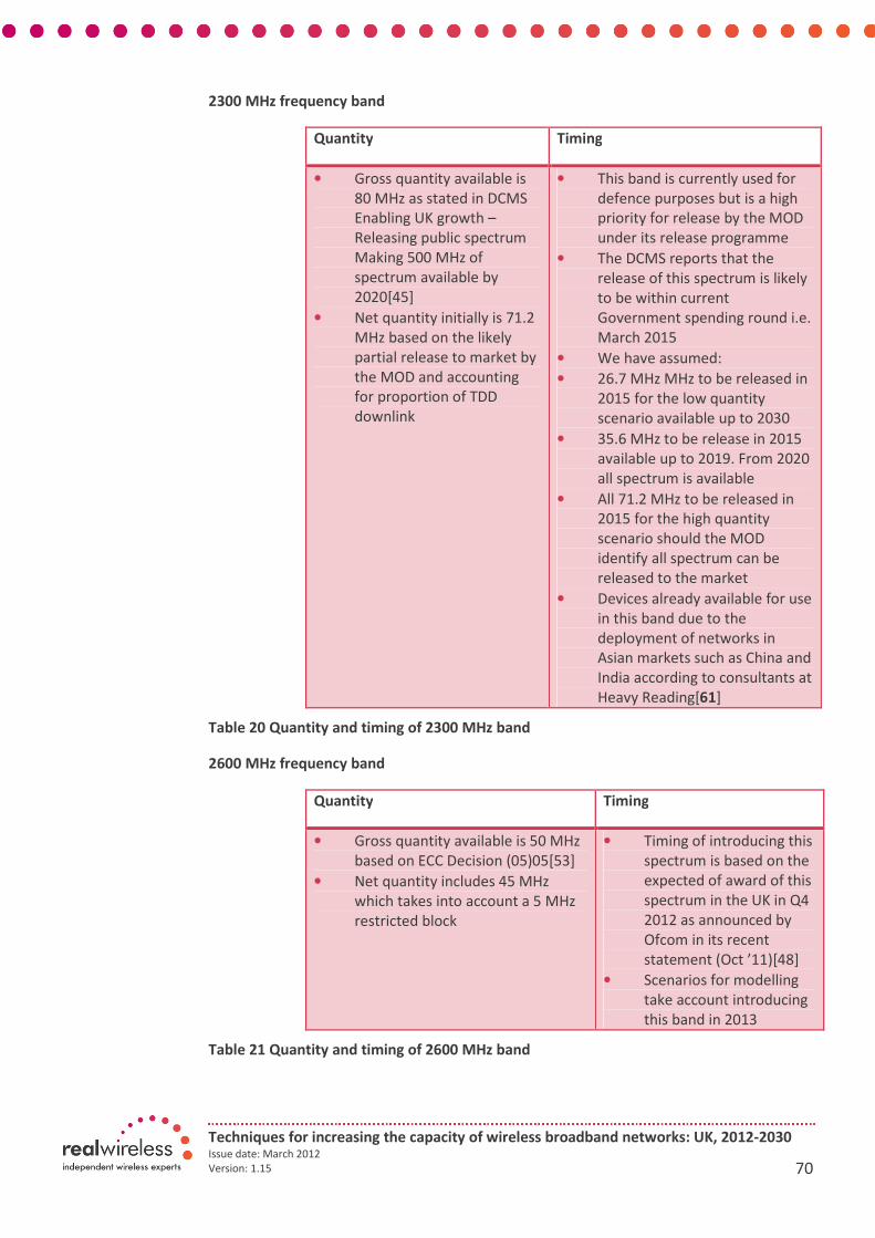
Techniques for increasing the capacity of wireless broadband networks: UK, 2012-2030 Issue date: March 2012
Version: 1.15 70
2300 MHz frequency band
Quantity Timing
• Gross quantity available is
80 MHz as stated in DCMS
Enabling UK growth –
Releasing public spectrum
Making 500 MHz of
spectrum available by
2020[45]
• Net quantity initially is 71.2
MHz based on the likely
partial release to market by
the MOD and accounting
for proportion of TDD
downlink
• This band is currently used for
defence purposes but is a high
priority for release by the MOD
under its release programme
• The DCMS reports that the
release of this spectrum is likely
to be within current
Government spending round i.e.
March 2015
• We have assumed:
• 26.7 MHz MHz to be released in
2015 for the low quantity
scenario available up to 2030
• 35.6 MHz to be release in 2015
available up to 2019. From 2020
all spectrum is available
• All 71.2 MHz to be released in
2015 for the high quantity
scenario should the MOD
identify all spectrum can be
released to the market
• Devices already available for use
in this band due to the
deployment of networks in
Asian markets such as China and
India according to consultants at
Heavy Reading[61]
Table 20 Quantity and timing of 2300 MHz band
2600 MHz frequency band
Quantity Timing
• Gross quantity available is 50 MHz
based on ECC Decision (05)05[53]
• Net quantity includes 45 MHz
which takes into account a 5 MHz
restricted block
• Timing of introducing this
spectrum is based on the
expected of award of this
spectrum in the UK in Q4
2012 as announced by
Ofcom in its recent
statement (Oct ’11)[48]
• Scenarios for modelling
take account introducing
this band in 2013
Table 21 Quantity and timing of 2600 MHz band

Techniques for increasing the capacity of wireless broadband networks: UK, 2012-2030 Issue date: March 2012
Version: 1.15 71
2700 -3100 MHz frequency band (High case only)
Quantity Timing
• Gross quantity available is
400 MHz based on globally
harmonised allocation for
radionavigation services for
both civil military. The band
is adjacent to the top of the
2.6 GHz IMT band
• Net quantity assumes the
use of 50 MHz of spectrum
out of the total for mobile
spectrum bands
• This band is currently used for
primary radar both aeronautical
and maritime. Radio navigation
is likely to remain in place for at
least 15 years, therefore re-
allocation will take place no
earlier than 2025
• We assume partial availability of
the band from 2025 onwards
for mobile broadband services
based on reallocation and re-
planning of radionavigation
services in the bottom portion
of the band thus creating a 50
MHz dividend
Table 22 Quantity and timing of 2700 MHz band
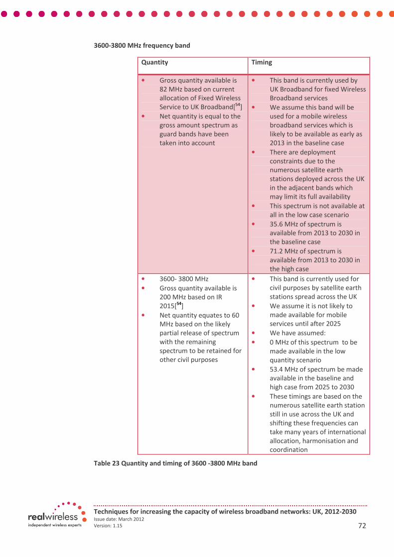
Techniques for increasing the capacity of wireless broadband networks: UK, 2012-2030 Issue date: March 2012
Version: 1.15 72
3600-3800 MHz frequency band
Quantity Timing
• Gross quantity available is
82 MHz based on current
allocation of Fixed Wireless
Service to UK Broadband[54
]
• Net quantity is equal to the
gross amount spectrum as
guard bands have been
taken into account
• This band is currently used by
UK Broadband for fixed Wireless
Broadband services
• We assume this band will be
used for a mobile wireless
broadband services which is
likely to be available as early as
2013 in the baseline case
• There are deployment
constraints due to the
numerous satellite earth
stations deployed across the UK
in the adjacent bands which
may limit its full availability
• This spectrum is not available at
all in the low case scenario
• 35.6 MHz of spectrum is
available from 2013 to 2030 in
the baseline case
• 71.2 MHz of spectrum is
available from 2013 to 2030 in
the high case
• 3600- 3800 MHz
• Gross quantity available is
200 MHz based on IR
2015[54
]
• Net quantity equates to 60
MHz based on the likely
partial release of spectrum
with the remaining
spectrum to be retained for
other civil purposes
• This band is currently used for
civil purposes by satellite earth
stations spread across the UK
• We assume it is not likely to
made available for mobile
services until after 2025
• We have assumed:
• 0 MHz of this spectrum to be
made available in the low
quantity scenario
• 53.4 MHz of spectrum be made
available in the baseline and
high case from 2025 to 2030
• These timings are based on the
numerous satellite earth station
still in use across the UK and
shifting these frequencies can
take many years of international
allocation, harmonisation and
coordination
Table 23 Quantity and timing of 3600 -3800 MHz band
Techniques for increasing the capacity of wireless broadband networks: UK, 2012-2030 Issue date: March 2012
Version: 1.15 73
3.4. Spectrum scenarios
The spectrum scenarios were derived so that a distinct spread of different quantities and
timings could be analysed to determine the impact of introducing new bands and
specifically the timing of introducing 700 MHz.
We proposed three scenarios which were based on the following factors:
• ‘Less’ Spectrum scenario: Represent existing incumbent mobile spectrum with
the quantity and timing as outlined in Table 12, Table 13 and Table 15 in the
section above. However, other more speculative spectrum bands such as 1452
MHz to 1492 MHz, 2.3 GHz, 3400 – 3600 MHz and 3600-3800 MHz each having
reduced spectrum quantities or no spectrum at all across the time frame
• Baseline case scenario: Representing existing incumbent mobile spectrum with
the quantity and timing as outlined in Table 12, Table 13 and Table 15 in the
section above. However, other more speculative spectrum bands such as 1452
MHz to 1492 MHz, 2.3 GHz, 3400 – 3600 MHz and 3600-3800 MHz each having
half or a third of the total spectrum quantities available across the time frame to
represent a more plausible representation of available spectrum
• ‘More’ Spectrum scenario: Representing existing incumbent mobile spectrum
with the quantity and timing as outlined in Table 12, Table 13 and Table 15 in the
section above. However, other more speculative spectrum bands such as 1452
MHz to 1492 MHz, 2.3 GHz, 3400 – 3600 MHz and 3600-3800 MHz each having
total spectrum quantities available from the point of release and available across
the time frame to represent a plausible yet more aggressive approach to
spectrum availability
• ‘Late public sector (PS)’ scenario: Representing existing incumbent mobile
spectrum where the 3.4 GHz and the 2.3 GHz bands are delayed relative to the
‘low’ case by a further 7 years and where the 2010-2025 MHz band is not
available. The proportion of spectrum which comes from public spectrum sources
varies amongst these scenarios from 11% (‘low PS’) via 22% (medium) to 24%
(high).
A summary chart of the spectrum scenarios can be seen in Figure 3-2 which shows the
spectrum quantities in each case evolving over time based on our assumptions. The total
quantity at the end of the period varies by as much as 340 MHz between the high case and
the low case. There is a smaller variation between the baseline (mid) case and the high case
due to increased proportion of spectrum becoming available in the middle and the end of
the time frame.
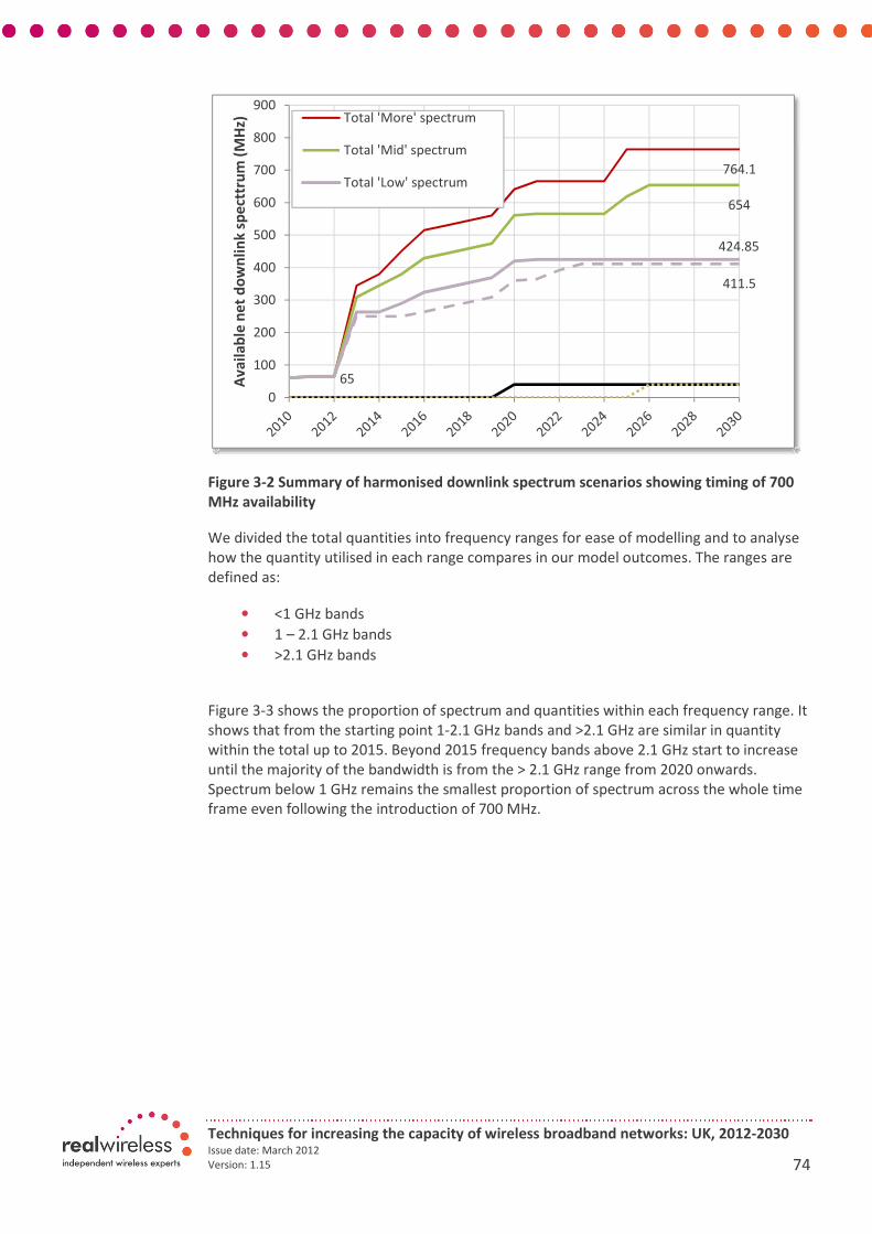
Techniques for increasing the capacity of wireless broadband networks: UK, 2012-2030 Issue date: March 2012
Version: 1.15 74
Figure 3-2 Summary of harmonised downlink spectrum scenarios showing timing of 700
MHz availability
We divided the total quantities into frequency ranges for ease of modelling and to analyse
how the quantity utilised in each range compares in our model outcomes. The ranges are
defined as:
• <1 GHz bands
• 1 – 2.1 GHz bands
• >2.1 GHz bands
Figure 3-3 shows the proportion of spectrum and quantities within each frequency range. It
shows that from the starting point 1-2.1 GHz bands and >2.1 GHz are similar in quantity
within the total up to 2015. Beyond 2015 frequency bands above 2.1 GHz start to increase
until the majority of the bandwidth is from the > 2.1 GHz range from 2020 onwards.
Spectrum below 1 GHz remains the smallest proportion of spectrum across the whole time
frame even following the introduction of 700 MHz.
764.1
654
424.85
65
411.5
0
100
200
300
400
500
600
700
800
900
Av
ail
ab
le n
et
do
wn
lin
k s
pe
cttr
um
(M
Hz) Total 'More' spectrum
Total 'Mid' spectrum
Total 'Low' spectrum

Techniques for increasing the capacity of wireless broadband networks: UK, 2012-2030 Issue date: March 2012
Version: 1.15 75
Figure 3-3 Total quantity of spectrum over time divided by frequency grouping - Baseline
scenario
Figure 3-4 shows the total quantity of spectrum over time with the frequency bands
grouped into paired and unpaired bands. The quantity of paired bands is greater across the
whole time frame compared to the unpaired bands. This suggests that in our baseline
scenario paired spectrum will continue to play a key role in delivery of mobile broadband
services with growing support from unpaired spectrum over time.
Figure 3-4 Total quantity of spectrum over time divided by paired and unpaired grouping
– Baseline scenario
Techniques for increasing the capacity of wireless broadband networks: UK, 2012-2030 Issue date: March 2012
Version: 1.15 76
The following set of tables outline the specific detail of the quantities and timing of each of
the frequency bands identified for use in the model. Each table shows the frequency band,
its respective frequency range (<1 GHz, 1-2.1 GHz, >2GHz), quantity or downlink, uplink and
total spectrum and the available bandwidth for each year.
It is noted that in 2012 2 x 5 MHz of the 900 MHz spectrum is available in London only and
not in the other study areas. This is based on the recent deployment of a UMTS900 network
by O2[62
] in London and we therefore assume data traffic will be deployed in one carrier in
this band initially.
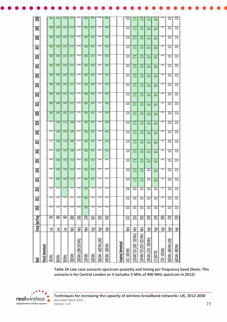
Techniques for increasing the capacity of wireless broadband networks: UK, 2012-2030 Issue date: March 2012
Version: 1.15 77
Table 24 Low case scenario spectrum quantity and timing per frequency band (Note: This
scenario is for Central London as it includes 5 MHz of 900 MHz spectrum in 2012)
Band
Group
Spot fr
equenc
y2010
2011
2012
2013
2014
2015
2016
2017
2018
2019
2020
2021
2022
2023
2024
2025
2026
2027
2028
2029
2030
Paired
, harm
onised
700 MH
zLow
7000
00
00
00
00
040
4040
4040
4040
4040
4040
800 MH
zLow
8000
00
3030
3030
3030
3030
3030
3030
3030
3030
3030
900 MH
zLow
9000
05
1010
1010
1520
2530
3535
3535
3535
3535
3535
1800 M
HzMe
d180
00
00
2222
2236
4656
6672
7272
7272
7272
7272
7272
1900 M
Hz (19
80-201
0 MHz)
Med
1900
00
00
00
00
00
00
00
00
00
00
0
2100 M
HzMe
d214
060
6060
6060
6060
6060
6060
6060
6060
6060
6060
6060
2600 M
HzHig
h265
50
00
7070
7070
7070
7070
7070
7070
7070
7070
7070
3400 M
Hz - 36
00 MH
z (UKB
)Hig
h350
00
00
00
00
00
00
00
00
00
00
00
3400 M
Hz - 36
00 MH
zHig
h350
00
00
00
020
2020
2020
2020
2020
2020
2020
2020
Unpai
red, H
armon
ised
1452 -1
492 MH
zMe
d147
20.0
0.00.0
0.00.0
0.00.0
0.00.0
0.00.0
0.00.0
0.00.0
0.00.0
0.00.0
0.00.0
2100 M
HZ TD
D (190
0 - 192
0 MHz)
Med
1910
0.00.0
0.017.
817.
817.
817.
817.
817.
817.
817.
817.
817.
817.
817.
817.
817.
817.
817.
817.
817.
8
2100 M
Hz TD
D (201
0 -2025
MHz)
Med
2018
0.00.0
0.013.
413.
413.
413.
413.
413.
413.
413.
413.
413.
413.
413.
413.
413.
413.
413.
413.
413.
4
2300 M
Hz (23
10 - 23
90 MH
z)Hig
h230
00.0
0.00.0
0.00.0
26.7
26.7
26.7
26.7
26.7
26.7
26.7
26.7
26.7
26.7
26.7
26.7
26.7
26.7
26.7
26.7
LTE 26
00 TD
DHig
h259
50.0
0.00.0
40.1
40.1
40.1
40.1
40.1
40.1
40.1
40.1
40.1
40.1
40.1
40.1
40.1
40.1
40.1
40.1
40.1
40.1
2700 -
3100 M
HzHig
h290
00
00
00
00
00
00
00
00
00
00
00
3600 M
Hz -38
00 MH
z (UKB)
High
3700
0.00.0
0.00.0
0.00.0
0.00.0
0.00.0
0.00.0
0.00.0
0.00.0
0.00.0
0.00.0
0.0
3600 M
Hz -38
00 MH
zHig
h370
00.0
0.00.0
0.00.0
0.00.0
0.00.0
0.00.0
0.00.0
0.00.0
0.00.0
0.00.0
0.00.0

Techniques for increasing the capacity of wireless broadband networks: UK, 2012-2030 Issue date: March 2012
Version: 1.15 78
Table 25 Baseline case scenario spectrum quantity and timing per frequency band (Note:
This scenario is for Central London as it includes 5 MHz of 900 MHz spectrum in 2012)
Band
Group
Spot fr
equenc
y2010
2011
2012
2013
2014
2015
2016
2017
2018
2019
2020
2021
2022
2023
2024
2025
2026
2027
2028
2029
2030
Paired
, harm
onised
700 MH
zLow
7000
00
00
00
00
040
4040
4040
4040
4040
4040
800 MH
zLow
8000
00
3030
3030
3030
3030
3030
3030
3030
3030
3030
900 MH
zLow
9000
05
1010
1010
1520
2530
3535
3535
3535
3535
3535
1800 M
HzMe
d180
00
00
2222
2236
4656
6672
7272
7272
7272
7272
7272
1900 M
Hz (19
80-201
0 MHz)
Med
1900
00
00
00
00
00
00
00
00
00
00
0
2100 M
HzMe
d214
060
6060
6060
6060
6060
6060
6060
6060
6060
6060
6060
2600 M
HzHig
h265
50
00
7070
7070
7070
7070
7070
7070
7070
7070
7070
3400 M
Hz - 36
00 MH
z (UKB)
High
3500
00
010
1010
1010
1010
1010
1010
1010
1010
1010
10
3400 M
Hz - 36
00 MH
zHig
h350
00
00
00
035
3535
3535
3535
3535
3570
7070
7070
Unpai
red, Ha
rmoni
sed
1452 -1
492 MH
zMe
d147
20
00
035.
635.
635.
635.
635.
635.
635.
635.
635.
635.
635.
635.
635.
635.
635.
635.
635.
6
2100 M
HZ TDD
(1900
- 1920
MHz)
Med
1910
00
017.
817.
817.
817.
817.
817.
817.
817.
817.
817.
817.
817.
817.
817.
817.
817.
817.
817.
8
2100 M
Hz TDD
(2010
-2025
MHz)
Med
2018
00
0.013.
413.
413.
413.
413.
413.
413.
413.
413.
413.
413.
413.
413.
413.
413.
413.
413.
413.
4
2300 M
Hz (23
10 - 23
90 MH
z)Hig
h230
00
00
00
35.6
35.6
35.6
35.6
35.6
71.2
71.2
71.2
71.2
71.2
71.2
71.2
71.2
71.2
71.2
71.2
2600M
Hz (un
paired
)Hig
h259
50
00
40.1
40.1
40.1
40.1
40.1
40.1
40.1
40.1
40.1
40.1
40.1
40.1
40.1
40.1
40.1
40.1
40.1
40.1
2700 -
3100 M
HzHig
h290
00
00
00
00
00
00
00
00
44.5
44.5
44.5
44.5
44.5
44.5
3600 M
Hz -38
00 MH
z (UKB)
High
3700
00
035.
635.
635.
635.
635.
635.
635.
635.
635.
635.
635.
635.
635.
635.
635.
635.
635.
635.
6
3600 M
Hz -38
00 MH
zHig
h370
00
00
00
00
00
00
00
00
53.4
53.4
53.4
53.4
53.4
53.4
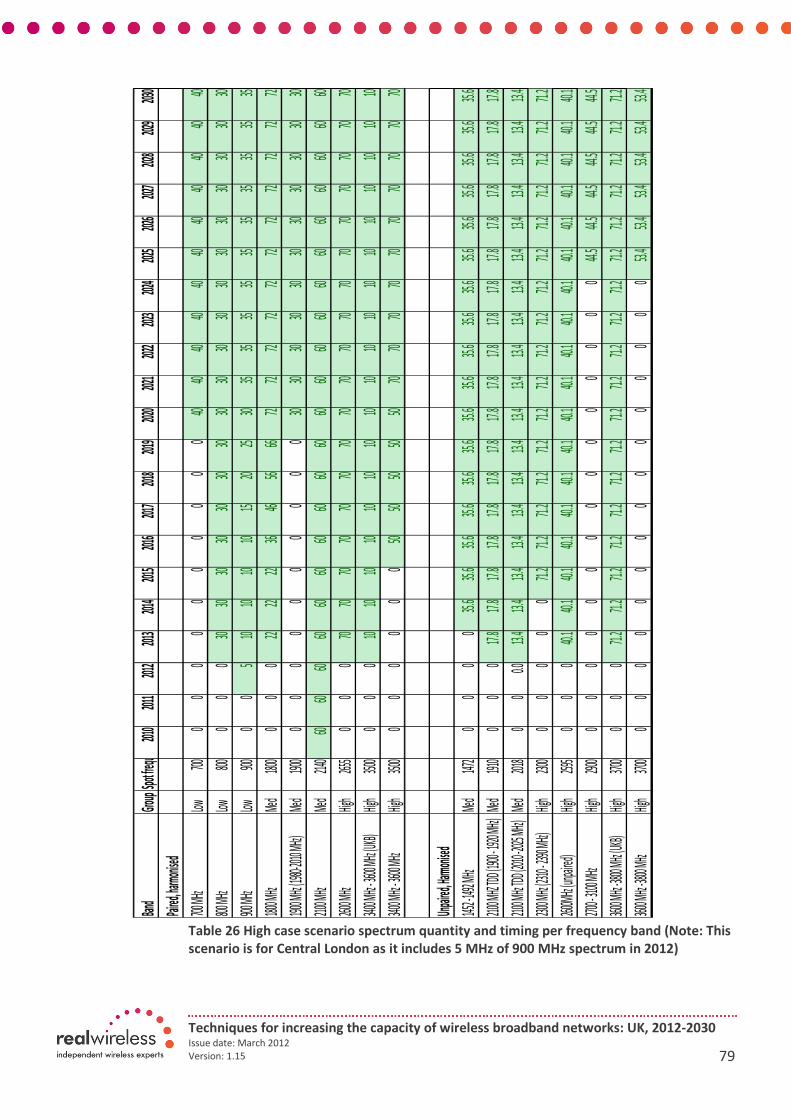
Techniques for increasing the capacity of wireless broadband networks: UK, 2012-2030 Issue date: March 2012
Version: 1.15 79
Table 26 High case scenario spectrum quantity and timing per frequency band (Note: This
scenario is for Central London as it includes 5 MHz of 900 MHz spectrum in 2012)
Band
Group
Spot fr
equenc
y2010
2011
2012
2013
2014
2015
2016
2017
2018
2019
2020
2021
2022
2023
2024
2025
2026
2027
2028
2029
2030
Paired
, harm
onised
700 MH
zLow
7000
00
00
00
00
040
4040
4040
4040
4040
4040
800 MH
zLow
8000
00
3030
3030
3030
3030
3030
3030
3030
3030
3030
900 MH
zLow
9000
05
1010
1010
1520
2530
3535
3535
3535
3535
3535
1800 M
HzMe
d180
00
00
2222
2236
4656
6672
7272
7272
7272
7272
7272
1900 M
Hz (19
80-201
0 MHz)
Med
1900
00
00
00
00
00
3030
3030
3030
3030
3030
30
2100 M
HzMe
d214
060
6060
6060
6060
6060
6060
6060
6060
6060
6060
6060
2600 M
HzHig
h265
50
00
7070
7070
7070
7070
7070
7070
7070
7070
7070
3400 M
Hz - 36
00 MH
z (UKB)
High
3500
00
010
1010
1010
1010
1010
1010
1010
1010
1010
10
3400 M
Hz - 36
00 MH
zHig
h350
00
00
00
050
5050
5050
7070
7070
7070
7070
7070
Unpai
red, Ha
rmoni
sed
1452 -1
492 MH
zMe
d147
20
00
035.
635.
635.
635.
635.
635.
635.
635.
635.
635.
635.
635.
635.
635.
635.
635.
635.
6
2100 M
HZ TDD
(1900
- 1920
MHz)
Med
1910
00
017.
817.
817.
817.
817.
817.
817.
817.
817.
817.
817.
817.
817.
817.
817.
817.
817.
817.
8
2100 M
Hz TDD
(2010
-2025
MHz)
Med
2018
00
0.013.
413.
413.
413.
413.
413.
413.
413.
413.
413.
413.
413.
413.
413.
413.
413.
413.
413.
4
2300 M
Hz (23
10 - 23
90 MH
z)Hig
h230
00
00
00
71.2
71.2
71.2
71.2
71.2
71.2
71.2
71.2
71.2
71.2
71.2
71.2
71.2
71.2
71.2
71.2
2600M
Hz (un
paired
)Hig
h259
50
00
40.1
40.1
40.1
40.1
40.1
40.1
40.1
40.1
40.1
40.1
40.1
40.1
40.1
40.1
40.1
40.1
40.1
40.1
2700 -
3100 M
HzHig
h290
00
00
00
00
00
00
00
00
44.5
44.5
44.5
44.5
44.5
44.5
3600 M
Hz -38
00 MH
z (UKB)
High
3700
00
071.
271.
271.
271.
271.
271.
271.
271.
271.
271.
271.
271.
271.
271.
271.
271.
271.
271.
2
3600 M
Hz -38
00 MH
zHig
h370
00
00
00
00
00
00
00
00
53.4
53.4
53.4
53.4
53.4
53.4
Techniques for increasing the capacity of wireless broadband networks: UK, 2012-2030 Issue date: March 2012
Version: 1.15 80
3.5. Modelling spectrum bands as a choice for supply
This section notes some assumptions made when considering the use of certain spectrum
bands in the model. The software model takes the spectrum as an input by way of total
quantity available in each year and by the end of the study period 17 frequency bands
(max) are available for use.
We have assumed a mix of devices that can support a sub set of the available frequency
bands in any one year thus making full use of the available bandwidth amongst the
population of mobiles. This does not require that individual mobiles can support all of the
bands, only that there is ultimately a reasonable match between capacity requirements and
frequency bands supported. We also assume the same mix of device types is used across all
bands.
Spectrum is made available as total bandwidth per year, however, the order of the choice
of spectrum bands is ranked based on the frequency band with highest maximum total
available bandwidth deployed first.

Techniques for increasing the capacity of wireless broadband networks: UK, 2012-2030 Issue date: March 2012
Version: 1.15 81
A4. Site Ranges
This annex explains the calculation of maximum site ranges for different combinations of
site types, technologies, clutter types and frequencies.
Figure 4-1: Illustration of site ranges for 1800 MHz
Figure 4-1 illustrates key concepts for site ranges: each site type has a different maximum
range for indoor and outdoor consumers. Macro sites have larger maximum ranges than
small cells. Other aspects such as the geotype of the study area and the carrier frequency
also impact the ranges as detailed in later sections. It can also be seen from the figure how
the site range reduces when serving indoor demand. This is mainly due to the building
penetration loss and location variability of user devices in the indoor environments.
Outdoor small cells with lower power transceivers have less site ranges compared with that
of macro cells as shown in Figure 4-1. In addition to site types, the maximum range of a site
is also dependent on other factors such as the bandwidth available to user devices and
minimum required cell edge throughput. Note however that the actual range of a site will
also be influenced by its capacity and by the interference scenario, so the calculations in
this section relate only to the maximum range of each site.
Macro cells with 3 sectors and 2 antennas
Small cells with 2 sectors and 2 antennas
Range indoor demands: 0.9
km
Range outdoor demands:
2.3 km
Range outdoor demands: 0.2 km Range indoor demands: 0.1 km
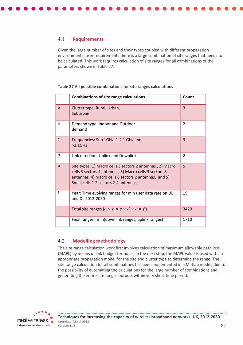
Techniques for increasing the capacity of wireless broadband networks: UK, 2012-2030 Issue date: March 2012
Version: 1.15 82
4.1 Requirements
Given the large number of sites and their types coupled with different propagation
environments, user requirements there is a large combination of site ranges that needs to
be calculated. This work requires calculation of site ranges for all combinations of the
parameters shown in Table 27.
Table 27 All possible combinations for site ranges calculations
Combinations of site range calculations Count
a Clutter type: Rural, Urban,
Suburban
3
b Demand type: Indoor and Outdoor
demand
2
c Frequencies: Sub 1GHz, 1-2.1 GHz and
>2.1GHz
3
d Link direction: Uplink and Downlink 2
e Site types: 1) Macro cells 3 sectors 2 antennas , 2) Macro
cells 3 sectors 4 antennas, 3) Macro cells 3 sectors 8
antennas, 4) Macro cells 6 sectors 2 antennas, and 5)
Small cells 1-2 sectors 2-4 antennas
5
f Year: Time evolving ranges for min user data rate on UL
and DL 2012-2030
19
Total site ranges (� × � × � × � × � × �) 3420
Final ranges= min(downlink ranges, uplink ranges) 1710
4.2 Modelling methodology
The site range calculation work first involves calculation of maximum allowable path loss
(MAPL) by means of link budget formulas. In the next step, the MAPL value is used with an
appropriate propagation model for the site and clutter type to determine the range. The
site range calculation for all combinations has been implemented in a Matlab model, due to
the possibility of automating the calculations for the large number of combinations and
generating the entire site ranges outputs within very short time period.

Techniques for increasing the capacity of wireless broadband networks: UK, 2012-2030 Issue date: March 2012
Version: 1.15 83
The whole site range calculations work can also be summarised in the steps as follows:
1. Select a year from the range 2012-2030
2. For the selected year:
2.1. Obtain the cell edge throughput requirements in Mbps, minimum
user device bandwidth, SINR cut off values
2.2. Select a combination of parameters
2.3. Calculate maximum allowable path loss (MAPL) for the selected
combination
2.4. Using the MAPL and selected combination calculate maximum
range as minimum of the associated uplink and downlink ranges
2.5. Repeat for all parameter combinations
3. While year<2031, run steps 1 and 2
The above steps give a total of 3420 site ranges as shown in Table 27 where 1710 ranges
are for the downlink transmissions and the other 1710 ranges are for the uplink
transmissions. The final site ranges are obtained from the minimum of the downlink and
uplink site ranges.
4.2.1 Flow charts
Flow charts of steps involved in the calculation are shown in Figure 4-2 and Figure 4-3 for
the MAPL and site range calculations, respectively.
4.2.1.1 Link Budget
Figure 4-2 shows the flow diagram of link budget calculation algorithm that runs the steps
to give MAPL value for each combination shown in Table 28 at each run. For example, when
site type is macro cells of 3 sectors 2 antennas, frequency is 1-2.1GHz, demand is indoor
and link direction is downlink, the algorithm uses these inputs to selection list of
parameters and assumptions in the link budget formulas to give the MAPL value for that
scenario.
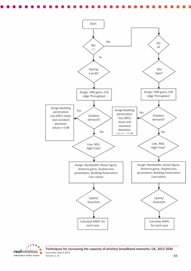
Techniques for increasing the capacity of wireless broadband networks: UK, 2012-2030 Issue date: March 2012
Version: 1.15 84
Start
Ma
cro
Sm
all
Outdoor
demand?
Assign:Building
penetration
loss (BPL) mean
and standard
deviation
values = 0 dB
Low, Mid,
High Freq?
Assign: Bandwidth, Noise Figure,
Antenna gains, shadow loss
parameters, Building Penetration
Loss values
Uplink/
Downlink
?
Calculate MAPL for
each case
SiteTyp
e (a-d)?
Assign: SNR gains, Cell
edge Throughput
Outdoor
demand?
Low, Mid,
High Freq?
Uplink/
Downlink
Calculate MAPL
for each case
Site
type?
Assign: SNR gains, Cell
edge Throughput
No
Ye
Yes
No
Assign:Building
penetration
loss (BPL)
mean and
standard
deviation
values = 0 dB
Assign: Bandwidth, Noise Figure,
Antenna gains, shadow loss
parameters, Building Penetration
Loss values
Yes
No
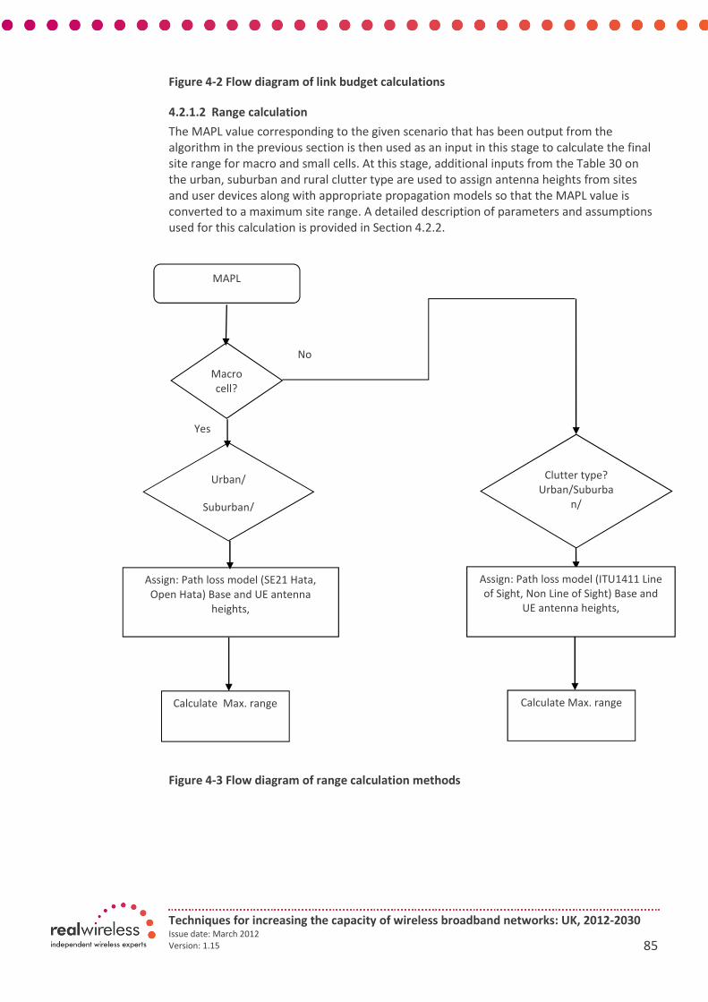
Techniques for increasing the capacity of wireless broadband networks: UK, 2012-2030 Issue date: March 2012
Version: 1.15 85
Figure 4-2 Flow diagram of link budget calculations
4.2.1.2 Range calculation
The MAPL value corresponding to the given scenario that has been output from the
algorithm in the previous section is then used as an input in this stage to calculate the final
site range for macro and small cells. At this stage, additional inputs from the Table 30 on
the urban, suburban and rural clutter type are used to assign antenna heights from sites
and user devices along with appropriate propagation models so that the MAPL value is
converted to a maximum site range. A detailed description of parameters and assumptions
used for this calculation is provided in Section 4.2.2.
Figure 4-3 Flow diagram of range calculation methods
Yes
No
MAPL
Macro
cell?
Calculate Max. range
Urban/
Suburban/
Assign: Path loss model (SE21 Hata,
Open Hata) Base and UE antenna
heights,
Calculate Max. range
Clutter type?
Urban/Suburba
n/
Assign: Path loss model (ITU1411 Line
of Sight, Non Line of Sight) Base and
UE antenna heights,
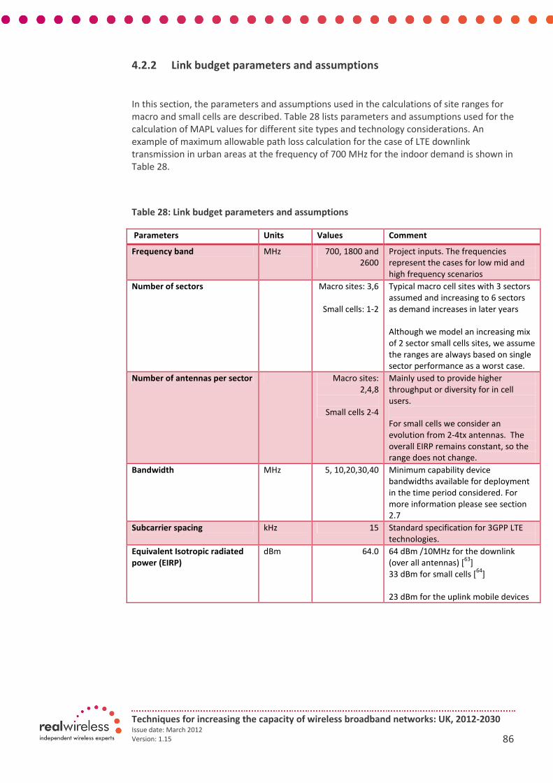
Techniques for increasing the capacity of wireless broadband networks: UK, 2012-2030 Issue date: March 2012
Version: 1.15 86
4.2.2 Link budget parameters and assumptions
In this section, the parameters and assumptions used in the calculations of site ranges for
macro and small cells are described. Table 28 lists parameters and assumptions used for the
calculation of MAPL values for different site types and technology considerations. An
example of maximum allowable path loss calculation for the case of LTE downlink
transmission in urban areas at the frequency of 700 MHz for the indoor demand is shown in
Table 28.
Table 28: Link budget parameters and assumptions
Parameters Units Values Comment
Frequency band MHz 700, 1800 and
2600
Project inputs. The frequencies
represent the cases for low mid and
high frequency scenarios
Number of sectors Macro sites: 3,6
Small cells: 1-2
Typical macro cell sites with 3 sectors
assumed and increasing to 6 sectors
as demand increases in later years
Although we model an increasing mix
of 2 sector small cells sites, we assume
the ranges are always based on single
sector performance as a worst case.
Number of antennas per sector Macro sites:
2,4,8
Small cells 2-4
Mainly used to provide higher
throughput or diversity for in cell
users.
For small cells we consider an
evolution from 2-4tx antennas. The
overall EIRP remains constant, so the
range does not change.
Bandwidth MHz 5, 10,20,30,40 Minimum capability device
bandwidths available for deployment
in the time period considered. For
more information please see section
2.7
Subcarrier spacing kHz 15 Standard specification for 3GPP LTE
technologies.
Equivalent Isotropic radiated
power (EIRP)
dBm 64.0 64 dBm /10MHz for the downlink
(over all antennas) [63
]
33 dBm for small cells [64
]
23 dBm for the uplink mobile devices

Techniques for increasing the capacity of wireless broadband networks: UK, 2012-2030 Issue date: March 2012
Version: 1.15 87
Transmit antenna gain dBi 15 for 700 MHz,
18 for 1800
MHz,
19.1 for 2600
MHz
Assumption, Kathrein 742 265 65
antenna specifications [65
]. For 700,
2600 MHz extrapolated from Kathrein
742 265 65 antenna specifications
6 dB for small cells [66
]
In the reverse link the transmit gain
also corresponds to receive antenna
gains.
Transmit cable, combiner and
connector losses
dB 0.0 Assumption, no loss due to cables,
combiners and connector consistent
with [66
]
This losses also correspond to receive
cable, combiner and connector losses
for the uplink
Receiver antenna gain dB 0 Assumption, no receive antenna gain
for user devices [67
]
This also corresponds to transmit
antenna gain for the user devices in
the uplink
Body loss (relative to free
space)
dB 0 Assumption, typical data connection
for laptops, tablets
Noise figure (NF) dB NF of user
devices
10 for 700 MHz,
9 for 1800 MHz,
9 for 2600 MHz
NF of cell sites
5
Noise of receivers affected by
frequency, allocated bandwidth,
duplex gap. Consistent with Ofcom
study in [68
]
Thermal noise density dBm/Hz -174 Constant
Thermal noise dBm -132 Noise power over the bandwidth of a
subcarrier
Background RSSI dBm -122 Thermal noise power added with
noise figure of the receiver
Interference degradation
margin
dB 4
1
Accounts for inter cell interference
with frequency reuse ratio of 1.
4.0 dB for the downlink [69
]
1 dB for the uplink [70
]
Cell edge throughput
requirement
Mbps 2
0.064
Cell edge throughput expected.
2Mbps the downlink and 64 kbps in
year 2012 [71
] and the requirement
increasing at 10% CAGR each year. See
Section 4.4.3
Cell loading factor % 85% Assumption, The loading is defined
here as the percentage of available
resources (frequency and time) used
to deliver download service to users
as in [67,68
]
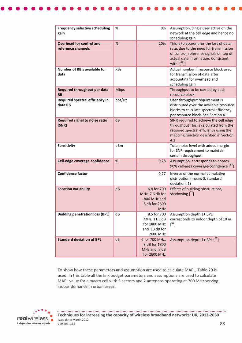
Techniques for increasing the capacity of wireless broadband networks: UK, 2012-2030 Issue date: March 2012
Version: 1.15 88
Frequency selective scheduling
gain
% 0% Assumption, Single user active on the
network at the cell edge and hence no
scheduling gain
Overhead for control and
reference channels
% 20% This is to account for the loss of data
rate, due to the need for transmission
of control, reference signals on top of
actual data information. Consistent
with [67
,]
Number of RB's available for
data
RBs Actual number if resource block used
for transmission of data after
accounting for overhead and
scheduling gain
Required throughput per data
RB
Mbps Throughput to be carried by each
resource block
Required spectral efficiency in
data RB
bps/Hz User throughput requirement is
distributed over the available resource
blocks to calculate spectral efficiency
per resource block. See Section 4.1
Required signal to noise ratio
(SNR)
dB SINR required to achieve the cell edge
throughput This is calculated from the
required spectral efficiency using the
mapping function described in Section
4.1
Sensitivity dBm Total noise level with added margin
for SNR requirement to maintain
certain throughput.
Cell-edge coverage-confidence % 0.78 Assumption, corresponds to approx.
90% cell-area coverage-confidence [67
]
Confidence factor 0.77 Inverse of the normal cumulative
distribution (mean: 0, standard
deviation: 1)
Location variability dB 6.8 for 700
MHz, 7.6 dB for
1800 MHz and
8 dB for 2600
MHz
Effects of building obstructions,
shadowing [72
]
Building penetration loss (BPL) dB 8.5 for 700
MHz, 11.3 dB
for 1800 MHz
and 13 dB for
2600 MHz
Assumption depth 1+ BPL,
corresponds to indoor depth of 10 m
[67
]
Standard deviation of BPL dB 6 for 700 MHz,
8 dB for 1800
MHz and 9 dB
for 2600 MHz
Assumption depth 1+ BPL [67
]
To show how these parameters and assumption are used to calculate MAPL, Table 29 is
used. In this table all the link budget parameters and assumptions are used to calculate
MAPL value for a macro cell with 3 sectors and 2 antennas operating at 700 MHz serving
indoor demands in urban areas.

Techniques for increasing the capacity of wireless broadband networks: UK, 2012-2030 Issue date: March 2012
Version: 1.15 89
Table 29: Link budget calculation example for a macro cell site with 3 sectors 2 transmit
antennas on the downlink of 700MHz serving indoor demands in urban areas
Parameter Symbol Units Values
Frequency band MHz 700
Receiver type Laptop/
Dongle
Number of antennas per sector AntCnt 2
Bandwidth BW MHz 20
Subcarrier Spacing, Receiver
filter BW
subBW kHz 15
EIRP/10MHz (over all antennas) EIRP10 dBm 64.0
Tx antenna gain TxGain dBi 15.0
Transmit Cable, Combiner and
Connector Losses
TxCCCL dB 0.0
No of occupied Subcarriers subCnt subcarriers ��� = (��/5) × 300 1200
No of occupied Resource Blocks RBcnt RBs ���� = ��� /12 100
EIRP in channel EIRPch dBm/15
kHz/ant
(DL)
�����ℎ= ����− 10�� 10(��� )
36.2
Receiver Antenna Gain RxGain dB 0
Receive Cable, Combiner and
Connector Losses
RxCCCL dB 0.0
Body Loss (relative to free space) BL dB 0.0
Noise figure NF dB 10.0
Thermal Noise Density thNsDns dBm/Hz -174
Thermal Noise thNs dBm ℎ!= ℎ!"�+ 10�� 10(���× 1000)
-132
Background RSSI RSSI dBm �$$� = !% + ℎ! -122
Interference Degradation Margin IM dB 4.0
Coverage obligation covObl Mbps 2.0
Network loading Loading % 85%
Frequency selective scheduling
gain
schGain % 0%
Overhead OHpc % 20%
Number of RB's available for
data
RBcntData RBs ���� "� � =
����&(���� × '���(� ×
(1 − )*+�))
68
Required throughput per data
RB
reqThPerDatRB Mbps &�,-ℎ��&"� ��= ��.)��/���� "� �
0.03
SINR cutoff SINRct dB -5
Required spectral efficiency in
data RB
reqSE bps/Hz &�,$�= &�,-ℎ��&"� �� × 1000
(��� ×
0.16

Techniques for increasing the capacity of wireless broadband networks: UK, 2012-2030 Issue date: March 2012
Version: 1.15 90
Required SNR reqSNR dB &�,$!�= max(10�� 10 32456789.;
− 1< , $�!�� )
-5
Sensitivity RxSens dBm �>$��= �$$� + &�,$!�
-127
Cell-edge coverage-confidence CellConf % 0.78
Confidence factor cf �� =��&?(�.(CellConf,0,1)
Normal inverse cumulative
distribution function,
mean=0, standard
deviation=1
0.77
Location variability (outdoor) Lv_sd dB 6.8
BPL BPL_mn dB 8.5
BPL SD BPL_sd dB 6
Fade margin (indoor) FM_in dB %@AB= ��'CB+ D'._�F + ��'_�F
15
Maximum path loss (indoor) MAPL dB @G�'= �����ℎ+ (�>H�(� − �>��'− �') − �@ − %@− �>$��
144
In Figure 4-5 and Figure 4-6 MAPL values for all the sites types for the case of downlink and
uplink, respectively for year 2012 are plotted. It can be seen from the figures that the MAPL
values for macrocell sites are higher than that of small cells. This is due mainly due to
higher EIRP and antenna gains of the macro cells sites. Comparing the MAPL values in
Figure 4-5 and Figure 4-6, it can be observed that MAPL does not increase for the downlink
of macro cells for additional antennas. Although techniques such as transmit diversity,
beamforming etc. can be used to improve the downlink performances, the gain in practice
from such techniques are still limited due to difficulties in accurate channel and direction of
arrival estimation and hence has not been considered in the link budget. In the uplink of
macro cell sites with more sectors e.g. from 3 to 6, improvement in the link is achieved due
to reduced impact of interference from other cells. Similarly having more antennas i.e. from
N = 2 to 4 and 8, improve the SNR gain of uplink transmission by 10 log 10 (!) dB even
without antenna diversity gain as signal energies from different can be coherently
combined [73
].
Figure 4-7 shows the evolution of minimum MAPL values from the both downlink and
uplink of cell sites.
Note that MAPL values generally reduce with time as the minimum throughput expectation
at the cell edge increases as discussed in Section 2.10. The periodic rise in MAPL values
corresponds to the years when the minimum bandwidth for user devices increases from 5
MHz in 2012 to 40 MHz in 2030 as discussed in Section 2.7. This leads to improved spectral
efficiency so that lower SINR is required to achieve the same throughput requirement. This,
in turn leads to increase in MAPL values as can also be seen from the calculations shown in
Table 29.

Techniques for increasing the capacity of wireless broadband networks: UK, 2012-2030 Issue date: March 2012
Version: 1.15 91
Figure 4-5 Maximum allowable path losses for downlink transmissions for different site
types in year 2012

Techniques for increasing the capacity of wireless broadband networks: UK, 2012-2030 Issue date: March 2012
Version: 1.15 92
Figure 4-6: Maximum allowable path losses for uplink transmissions for different site
types in year 2012
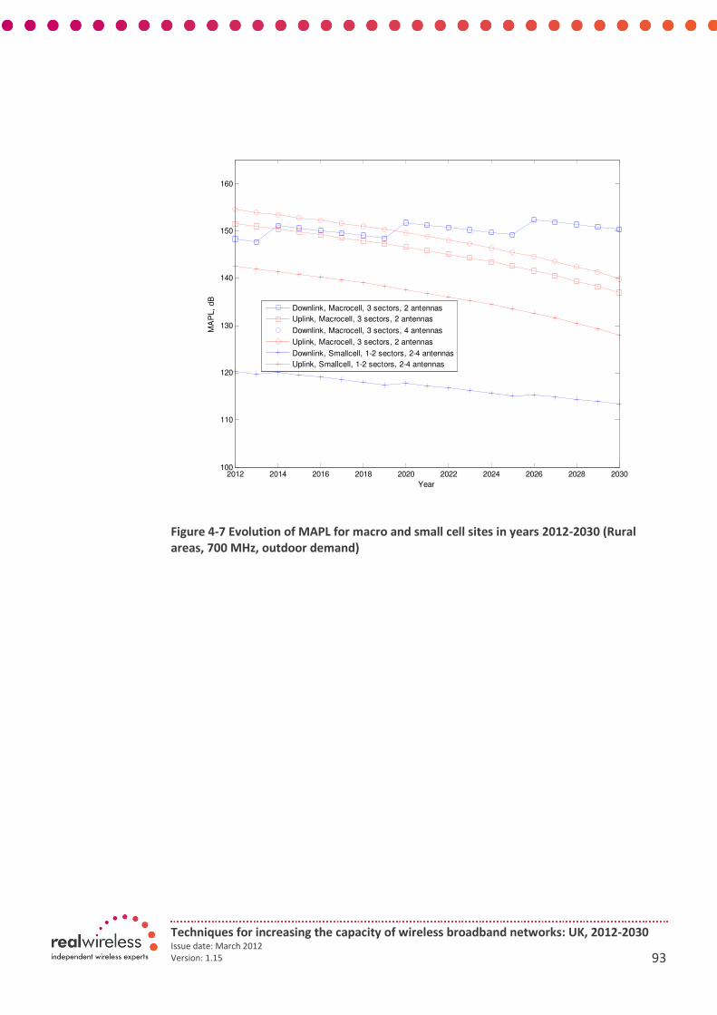
Techniques for increasing the capacity of wireless broadband networks: UK, 2012-2030 Issue date: March 2012
Version: 1.15 93
Figure 4-7 Evolution of MAPL for macro and small cell sites in years 2012-2030 (Rural
areas, 700 MHz, outdoor demand)
2012 2014 2016 2018 2020 2022 2024 2026 2028 2030100
110
120
130
140
150
160
Year
MA
PL,
dB
Downlink, Macrocell, 3 sectors, 2 antennas
Uplink, Macrocell, 3 sectors, 2 antennas
Downlink, Macrocell, 3 sectors, 4 antennas
Uplink, Macrocell, 3 sectors, 2 antennas
Downlink, Smallcell, 1-2 sectors, 2-4 antennas
Uplink, Smallcell, 1-2 sectors, 2-4 antennas
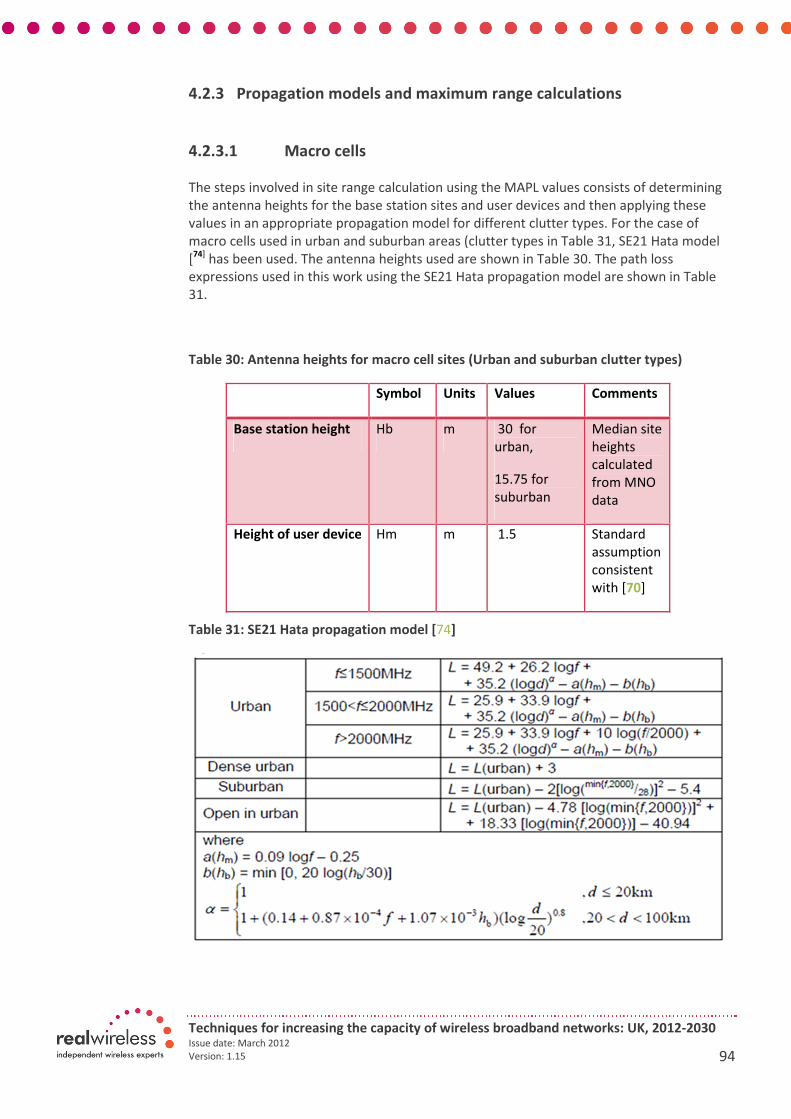
Techniques for increasing the capacity of wireless broadband networks: UK, 2012-2030 Issue date: March 2012
Version: 1.15 94
4.2.3 Propagation models and maximum range calculations
4.2.3.1 Macro cells
The steps involved in site range calculation using the MAPL values consists of determining
the antenna heights for the base station sites and user devices and then applying these
values in an appropriate propagation model for different clutter types. For the case of
macro cells used in urban and suburban areas (clutter types in Table 31, SE21 Hata model
[74]
has been used. The antenna heights used are shown in Table 30. The path loss
expressions used in this work using the SE21 Hata propagation model are shown in Table
31.
Table 30: Antenna heights for macro cell sites (Urban and suburban clutter types)
Symbol Units Values Comments
Base station height Hb m 30 for
urban,
15.75 for
suburban
Median site
heights
calculated
from MNO
data
Height of user device Hm m 1.5 Standard
assumption
consistent
with [70]
Table 31: SE21 Hata propagation model [74]

Techniques for increasing the capacity of wireless broadband networks: UK, 2012-2030 Issue date: March 2012
Version: 1.15 95
For the case of macro cells used in rural areas (clutter types in Table 31), the extended Hata
model for open areas as given in [74] has been used. The antenna heights used are shown
in Table 32.
Table 32: Antenna heights for macro cell sites (Rural clutter types)
Symbol Units Values Comments
Base station height Hb m 16.5 Median site heights
calculated from MNO
data
Height of user
device
Hm m 1.5 Standard assumption
consistent with [70]
4.2.3.2 Small cells
The site range calculation methodology for small cells is as follows. The antenna heights for
both cell sites and user devices are obtained as shown in Table 33. Next, using the MAPL
values the small cell sites, two sets of ranges corresponding to the scenarios of line of sight
(LOS) and non line of sight (NLOS) are calculated using the models in [75
].
Table 33: ITU 1411 outdoor LOS or NLOS model based on WINNER model for LOS
probability
Symbol Unit Values Comments
Base station height Hb M 5 for urban,
5 for suburban,
4 for rural
Median site heights
calculated from MNO
data
Height of user
device
Hm M 1.5 Standard assumption
consistent with [71]
To account for both LOS and NLOS propagation conditions in the final range calculation, the
models of LOS probabilities for different site types are given in the WINNER project [76] .
The following expressions from the models are used to calculate the LOS probabilities
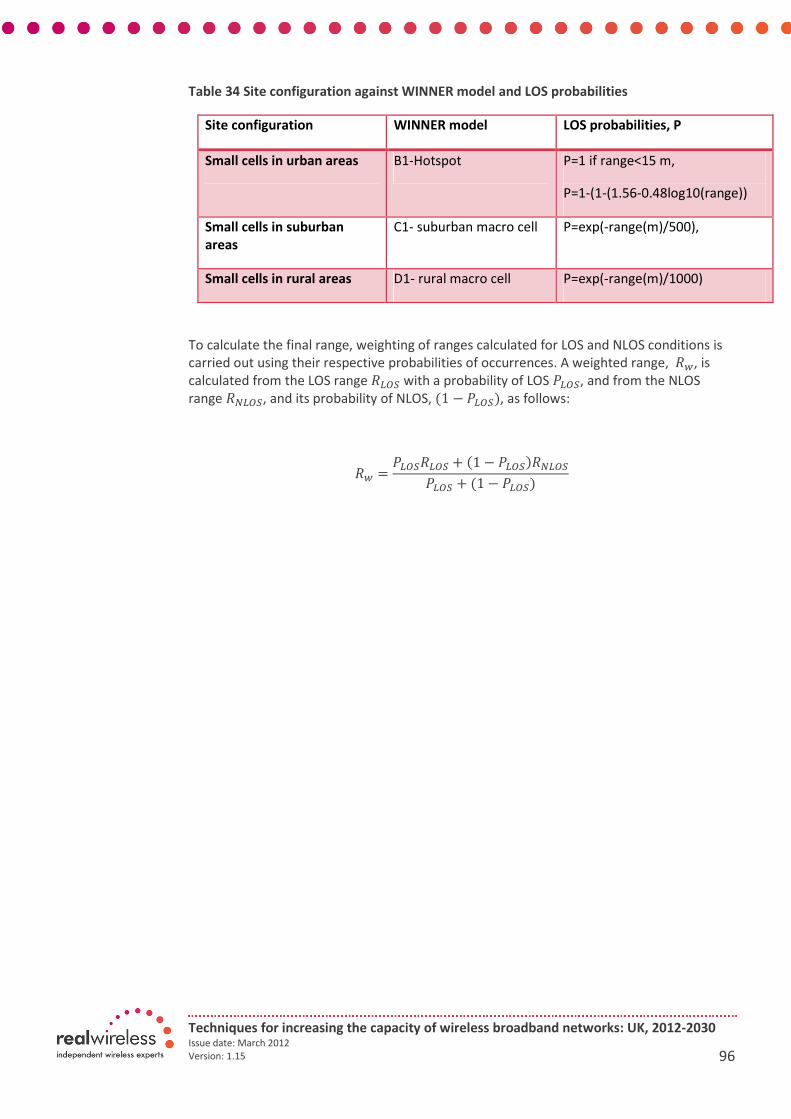
Techniques for increasing the capacity of wireless broadband networks: UK, 2012-2030 Issue date: March 2012
Version: 1.15 96
Table 34 Site configuration against WINNER model and LOS probabilities
Site configuration WINNER model LOS probabilities, P
Small cells in urban areas B1-Hotspot P=1 if range<15 m,
P=1-(1-(1.56-0.48log10(range))
Small cells in suburban
areas
C1- suburban macro cell P=exp(-range(m)/500),
Small cells in rural areas D1- rural macro cell P=exp(-range(m)/1000)
To calculate the final range, weighting of ranges calculated for LOS and NLOS conditions is
carried out using their respective probabilities of occurrences. A weighted range, �L, is
calculated from the LOS range �MN7 with a probability of LOS �MN7, and from the NLOS
range �OMN7, and its probability of NLOS, (1 − �MN7), as follows:
�L = �MN7�MN7 + (1 − �MN7)�OMN7�MN7 + (1 − �MN7)

Techniques for increasing the capacity of wireless broadband networks: UK, 2012-2030 Issue date: March 2012
Version: 1.15 97
4.3 Site Ranges
The final site ranges for the different site types for the year 2012 is plotted in Figure 4-8.
These results are obtained from the MAPL values as calculated in Table 29 and then
applying the propagation models according to the clutter types. It can be seen from the
figure that the macro cell sites offer significantly higher site ranges compared with small
cell sites. The low frequency sites provide higher ranges compared with higher frequency
sites for all cases. It is also clear from the figure that site ranges are significantly reduced
when serving the indoor demands. This is mainly due the building penetration loss as
discussed in Section 4.2.1.1.

Techniques for increasing the capacity of wireless broadband networks: UK, 2012-2030 Issue date: March 2012
Version: 1.15 98
Figure 4-8 Site ranges for minimum of uplink/downlink transmissions for different site
types in year 2012

Techniques for increasing the capacity of wireless broadband networks: UK, 2012-2030 Issue date: March 2012
Version: 1.15 99
Figure 4-9 shows the final site ranges for different site types operating in 700 MHz in rural
areas serving outdoor demands. Site ranges for other frequencies and propagation
scenarios also follow similar trends and hence are not shown here. The final site ranges are
obtained from both the downlink and uplink by selecting the one with minimum range for
each year. In has been discussed earlier that in the downlink, minimum bandwidth of user
devices increases over time from 5 MHz in 2012 to 40 MHz in 2030 (See Section 2.7). This
increase of bandwidth in different years leads to improvement in downlink site ranges. It
can be seen from Figure 4-9 that in 2012, site ranges for all macrocells are equal. In this
year, the limiting case from the downlink and uplink ranges has been the downlink ranges
since only 5 MHz of bandwidth is available for user devices. Hence, even if the uplink ranges
for macro cells 3 sectors and 8 antennas are much higher, the downlink ranges are selected
are final ranges. In year 2014, the device bandwidth increases to 10 MHz; this leads to
increase in ranges for all macro cell sites.
For macro cell sites with 3 sectors and 2 antennas, from 2014 the uplink ranges become
limiting cases and hence the ranges decrease each year till 2030. For macro cells with 3
sectors and 4 antennas and 6 sectors and 2 antennas have almost the same ranges. The
macro cell sites with 3 sectors and 8 antennas have the highest ranges, this is mainly due to
combination of the two factors: a) minimum user device bandwidth increasing in different
year till 2030 and hence increasing the downlink ranges, b) use of 8 antennas for the uplink
also leads to significant gain in the link budget and hence the high site ranges. Ultimately,
the uplink ranges become the limiting cases and the site ranges drop from year 2020
onwards.
Figure 4-9: Evolution of maximum site ranges for macro and small cell sites (Rural areas,
700 MHz, outdoor demands) in years 2012-2030
2012 2014 2016 2018 2020 2022 2024 2026 2028 20300
5
10
15
20
25
30
Year
Maxim
um
ran
ge,
km
Macrocell, 3 sectors, 2 antennas
Macrocell, 3 sectors, 4 antennas
Macrocell, 3 sectors, 8 antennas
Macrocell, 6 sectors, 2 antennas
Smallcell, 1-2 sectors, 2-4 antennas

Techniques for increasing the capacity of wireless broadband networks: UK, 2012-2030 Issue date: March 2012
Version: 1.15 100
The effects of varying site ranges over time can potentially introduce randomness into the
deployment of sites. For example if one particular site does not get upgraded early in the
timeframe and another one does, then the upgraded site has an advantage in terms of
range from that point in time and can create an imbalance later in the timeframe.
Therefore, in order to minimise potentially misleading effects in the results we decided to
set all site ranges across types to the same level. Figure 4-10 shows the site ranges across
all the environments that remain static over time from 2012 through to 2030.
Figure 4-10 Site range variation between environments (Demand, geotype and frequency
group)
In Out In Out In Out In Out In Out In Out In Out In Out In Out
Urb Urb Sub Sub Rur Rur Urb Urb Sub Sub Rur Rur Urb Urb Sub Sub Rur Rur
High High High High High High Med Med Med Med Med Med Low Low Low Low Low Low
Macro3sec2tx 0.69 1.98 1.17 2.86 3.44 8.43 0.91 2.26 1.66 3.55 5.61 12.01 2.72 5.31 3.77 6.37 12.68 21.46
Macro3sec4tx 0.69 1.98 1.17 2.86 3.44 8.43 0.91 2.26 1.66 3.55 5.61 12.01 2.72 5.31 3.77 6.37 12.68 21.46
Macro3sec6tx 0.69 1.98 1.17 2.86 3.44 8.43 0.91 2.26 1.66 3.55 5.61 12.01 2.72 5.31 3.77 6.37 12.68 21.46
Macro6sec2tx 0.69 1.98 1.17 2.86 3.44 8.43 0.91 2.26 1.66 3.55 5.61 12.01 2.72 5.31 3.77 6.37 12.68 21.46
Small Cell 0.09 0.20 0.35 0.41 0.45 0.79 0.10 0.23 0.41 0.42 0.48 0.76 0.20 0.38 0.43 0.48 0.57 0.75
0
5
10
15
20
25
Range Variation over Environment and Frequency in 2012
Macro3sec2tx
Macro3sec4tx
Macro3sec6tx
Macro6sec2tx
Small CellFrequency
Demand location
Geotype
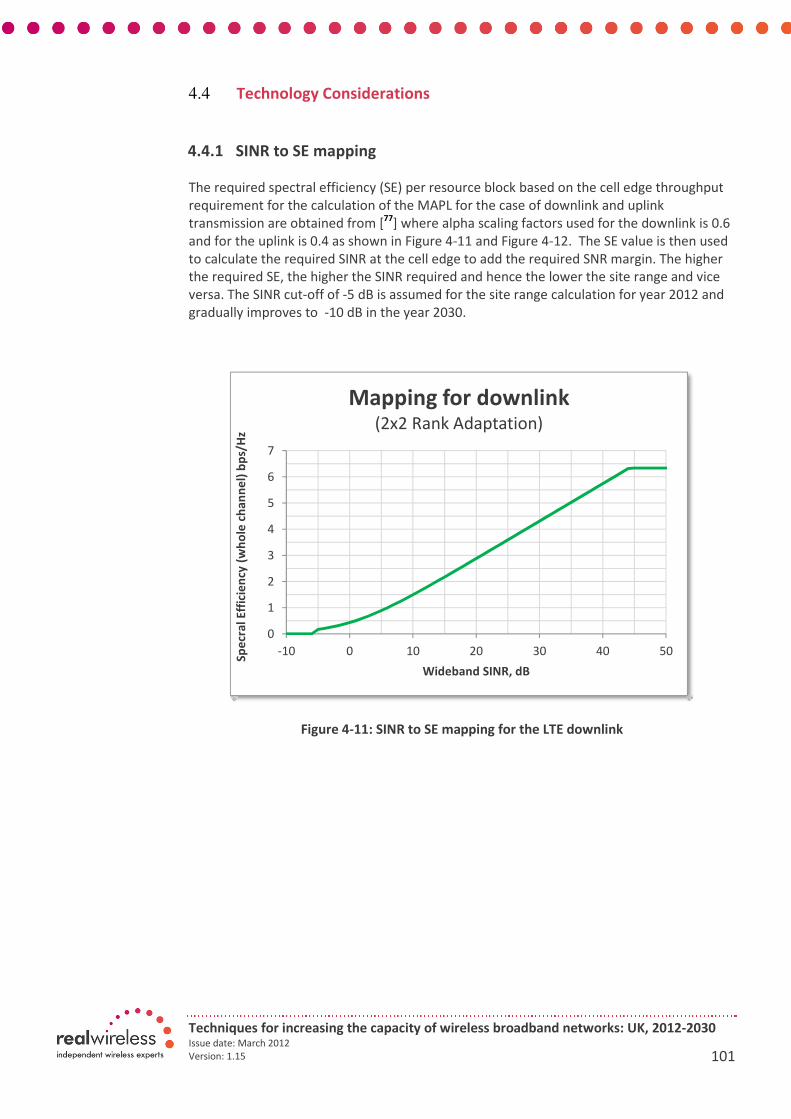
Techniques for increasing the capacity of wireless broadband networks: UK, 2012-2030 Issue date: March 2012
Version: 1.15 101
4.4 Technology Considerations
4.4.1 SINR to SE mapping
The required spectral efficiency (SE) per resource block based on the cell edge throughput
requirement for the calculation of the MAPL for the case of downlink and uplink
transmission are obtained from [77
] where alpha scaling factors used for the downlink is 0.6
and for the uplink is 0.4 as shown in Figure 4-11 and Figure 4-12. The SE value is then used
to calculate the required SINR at the cell edge to add the required SNR margin. The higher
the required SE, the higher the SINR required and hence the lower the site range and vice
versa. The SINR cut-off of -5 dB is assumed for the site range calculation for year 2012 and
gradually improves to -10 dB in the year 2030.
Figure 4-11: SINR to SE mapping for the LTE downlink
0
1
2
3
4
5
6
7
-10 0 10 20 30 40 50
Sp
ecr
al
Eff
icie
ncy
(w
ho
le c
ha
nn
el)
bp
s/H
z
Wideband SINR, dB
Mapping for downlink (2x2 Rank Adaptation)
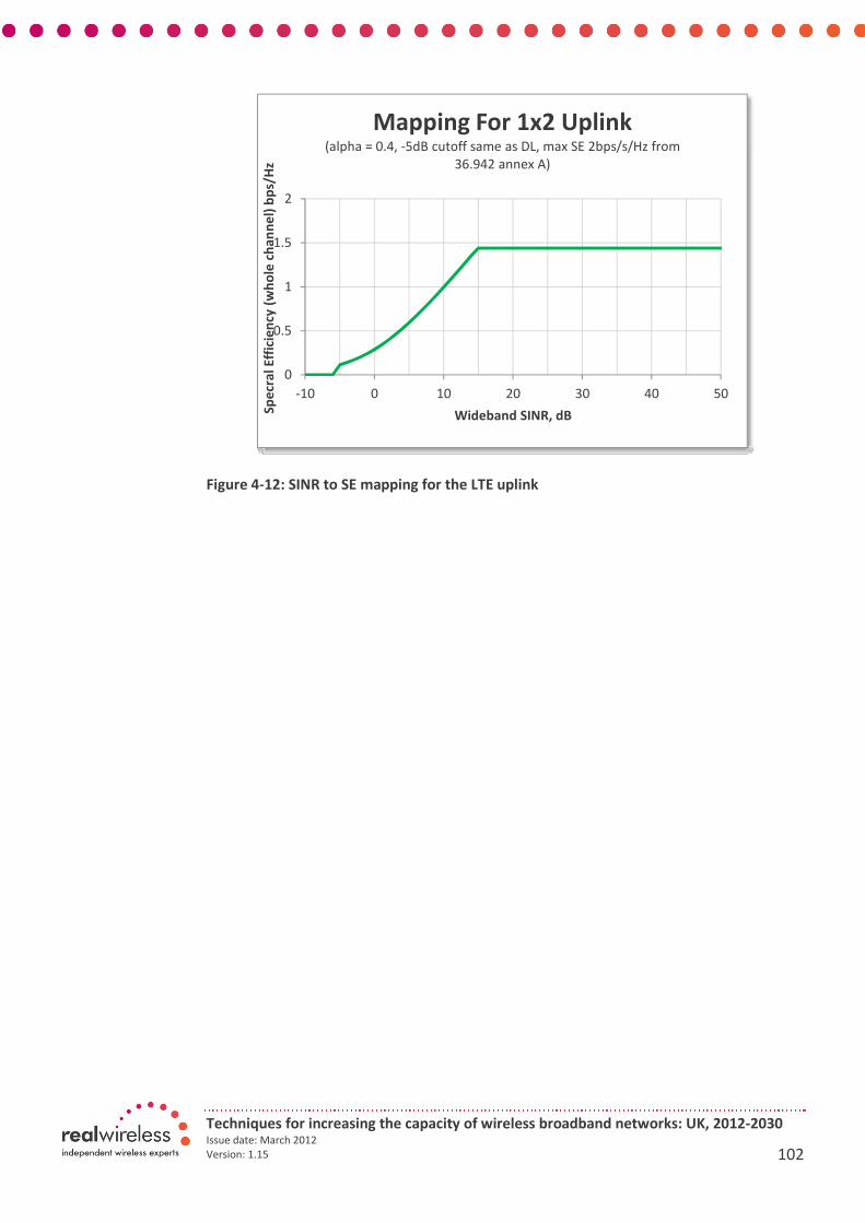
Techniques for increasing the capacity of wireless broadband networks: UK, 2012-2030 Issue date: March 2012
Version: 1.15 102
Figure 4-12: SINR to SE mapping for the LTE uplink
0
0.5
1
1.5
2
-10 0 10 20 30 40 50
Sp
ecr
al
Eff
icie
ncy
(w
ho
le c
ha
nn
el)
bp
s/H
z
Wideband SINR, dB
Mapping For 1x2 Uplink (alpha = 0.4, -5dB cutoff same as DL, max SE 2bps/s/Hz from
36.942 annex A)
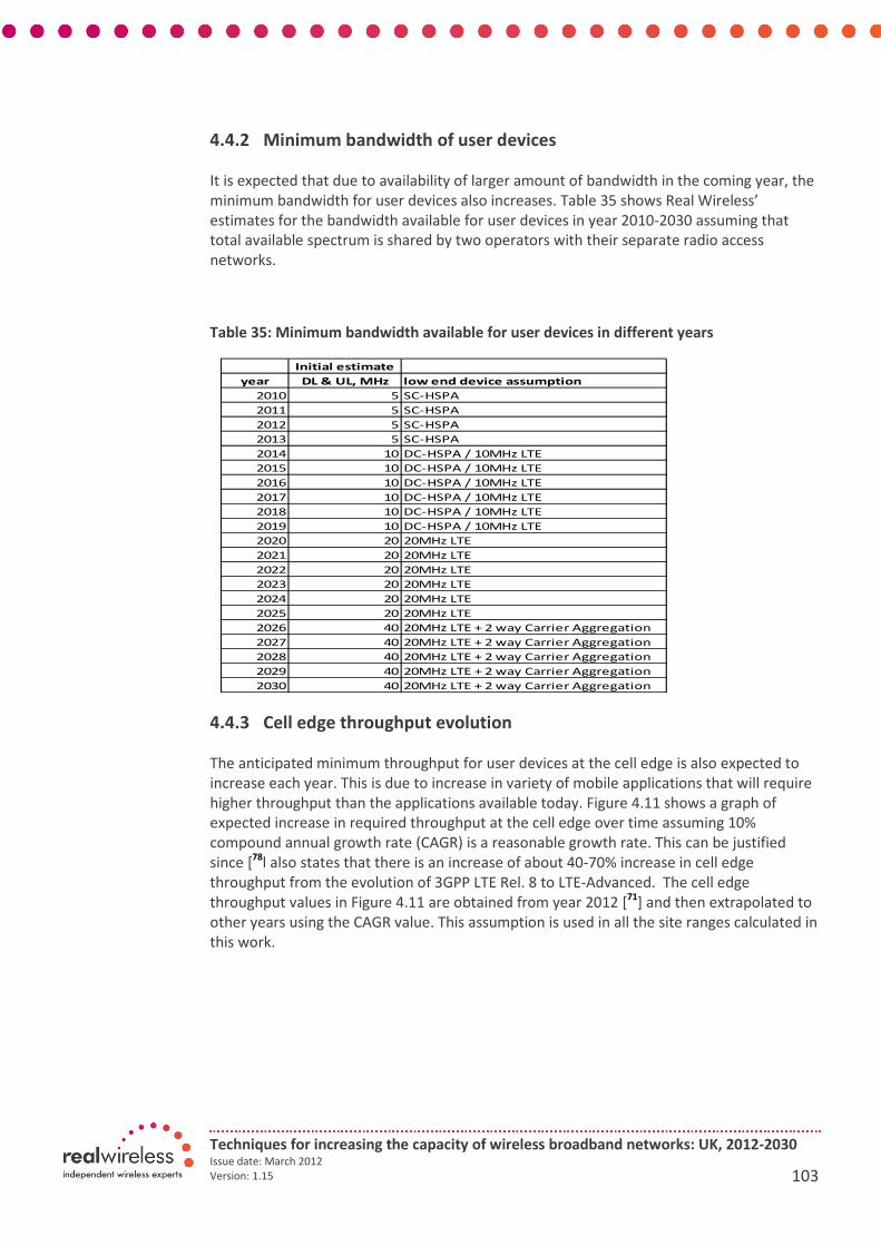
Techniques for increasing the capacity of wireless broadband networks: UK, 2012-2030 Issue date: March 2012
Version: 1.15 103
4.4.2 Minimum bandwidth of user devices
It is expected that due to availability of larger amount of bandwidth in the coming year, the
minimum bandwidth for user devices also increases. Table 35 shows Real Wireless’
estimates for the bandwidth available for user devices in year 2010-2030 assuming that
total available spectrum is shared by two operators with their separate radio access
networks.
Table 35: Minimum bandwidth available for user devices in different years
4.4.3 Cell edge throughput evolution
The anticipated minimum throughput for user devices at the cell edge is also expected to
increase each year. This is due to increase in variety of mobile applications that will require
higher throughput than the applications available today. Figure 4.11 shows a graph of
expected increase in required throughput at the cell edge over time assuming 10%
compound annual growth rate (CAGR) is a reasonable growth rate. This can be justified
since [78
l also states that there is an increase of about 40-70% increase in cell edge
throughput from the evolution of 3GPP LTE Rel. 8 to LTE-Advanced. The cell edge
throughput values in Figure 4.11 are obtained from year 2012 [71
] and then extrapolated to
other years using the CAGR value. This assumption is used in all the site ranges calculated in
this work.
Initial estimate
year DL & UL, MHz low end device assumption
2010 5 SC-HSPA
2011 5 SC-HSPA
2012 5 SC-HSPA
2013 5 SC-HSPA
2014 10 DC-HSPA / 10MHz LTE
2015 10 DC-HSPA / 10MHz LTE
2016 10 DC-HSPA / 10MHz LTE
2017 10 DC-HSPA / 10MHz LTE
2018 10 DC-HSPA / 10MHz LTE
2019 10 DC-HSPA / 10MHz LTE
2020 20 20MHz LTE
2021 20 20MHz LTE
2022 20 20MHz LTE
2023 20 20MHz LTE
2024 20 20MHz LTE
2025 20 20MHz LTE
2026 40 20MHz LTE + 2 way Carrier Aggregation
2027 40 20MHz LTE + 2 way Carrier Aggregation
2028 40 20MHz LTE + 2 way Carrier Aggregation
2029 40 20MHz LTE + 2 way Carrier Aggregation
2030 40 20MHz LTE + 2 way Carrier Aggregation

Techniques for increasing the capacity of wireless broadband networks: UK, 2012-2030 Issue date: March 2012
Version: 1.15 104
Figure 4-13: Cell edge minimum throughput evolution over time per user device

Techniques for increasing the capacity of wireless broadband networks: UK, 2012-2030 Issue date: March 2012
Version: 1.15 105
A5. Demand assessment
5.1 Introduction
The demand assessment has drawn upon a wide range of published data and forecasts to
build up a model of demand growth extended over the 18 year study timeframe that could
be mapped on to regional study areas. Population, postcode and route (road and rail) data
inputs were used for the demand points to produce representative spatial forecasts in each
case. Figure 5-1 presents an example demand map for rural Lincolnshire which was
produced using the software model that incorporates the demand distribution data
mapped across a set of geographical demand points.
Figure 5-1 Demand map in 2012 for rural Lincolnshire across population, postcodes and
road/rail
As explained in section 3.4 the input data and approach used to determine the demand was
built up from a set of required distributions using independent analyst, vendor and
operator demand forecasts. This data was gathered according to each distribution and
analysed to produce a set of plausible growth assumptions for the demand inputs.
Techniques for increasing the capacity of wireless broadband networks: UK, 2012-2030 Issue date: March 2012
Version: 1.15 106
The following set of distributions were individually analysed to build up the demand data
into a growth chart for the low, mid and high cases:
• Volume of traffic generated by device types
• Penetration of devices amongst the general population
• Distribution of traffic amongst individual users
• Location of traffic generated such indoors at home or on the move
• Variation of traffic generated at particular times of day
The blend of each of the above attributes forms the input data used to generate the
demand spread across each of the geographical locations.
This annex outlines the general approach, methodology and assumptions used to derive a
set of demand growth scenarios which in turn provide the demand challenges for the
mobile network deployment (supply) modelling and capacity dimensioning. Ultimately it is
the magnitude of demand that dictates the capacity that is required to satisfy it, therefore
it was essential to ensure credible and plausible demand scenarios were produced for
modelling.
In this study we have used the updated forecasts such as the widely quoted forecasts by
Cisco[79
] and the recent (Nov 2011) published forecast by Ericsson[80
] which now includes
data on the impact of tablet devices such as the iPad and embedded modules which are
now becoming a feature of more recent analyses.
5.2 General approach
Our general approach is outlined in Figure 5-2, showing the high level flowchart and inputs
required to build up the demand distribution. The inputs in the blue boxes represent the
geographical data which includes the delivery addresses of both residential locations and
businesses according to postcode, road and rail routes, special locations such as airports,
shopping centres and stadia and geotype (Urban, Suburban and Rural).
The inputs in the orange boxes represent the various distributions that make up the
attributes of demand as listed in section 5.1. Combining these attributes provides a total
volume of traffic that can be defined by the population of the study areas and quantified
based on three separate busy hours which we determine in our analysis (described in more
detail in section 5.3).
The processing stage is where we combine the distributions and the geographical data to
produce a set of aggregated demand values that can be mapped on to the study area
demand points by weighting the proportion of traffic according to the time of day across
the different locations.
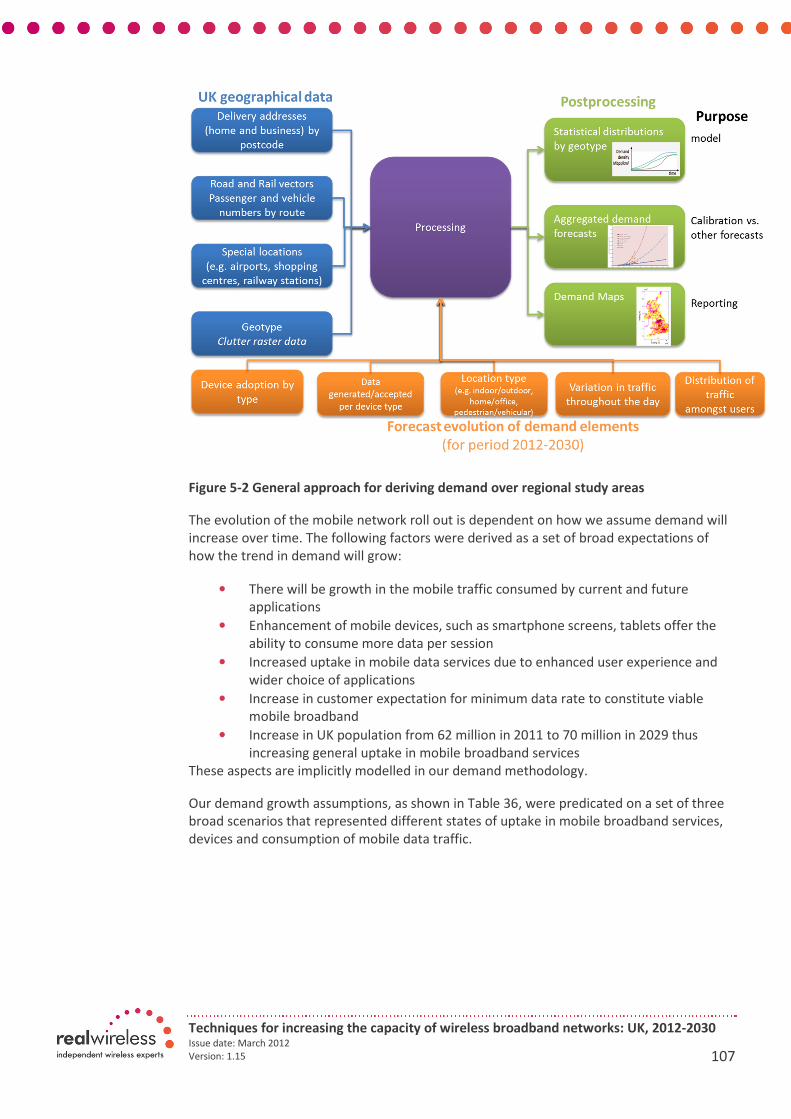
Techniques for increasing the capacity of wireless broadband networks: UK, 2012-2030 Issue date: March 2012
Version: 1.15 107
Figure 5-2 General approach for deriving demand over regional study areas
The evolution of the mobile network roll out is dependent on how we assume demand will
increase over time. The following factors were derived as a set of broad expectations of
how the trend in demand will grow:
• There will be growth in the mobile traffic consumed by current and future
applications
• Enhancement of mobile devices, such as smartphone screens, tablets offer the
ability to consume more data per session
• Increased uptake in mobile data services due to enhanced user experience and
wider choice of applications
• Increase in customer expectation for minimum data rate to constitute viable
mobile broadband
• Increase in UK population from 62 million in 2011 to 70 million in 2029 thus
increasing general uptake in mobile broadband services
These aspects are implicitly modelled in our demand methodology.
Our demand growth assumptions, as shown in Table 36, were predicated on a set of three
broad scenarios that represented different states of uptake in mobile broadband services,
devices and consumption of mobile data traffic.
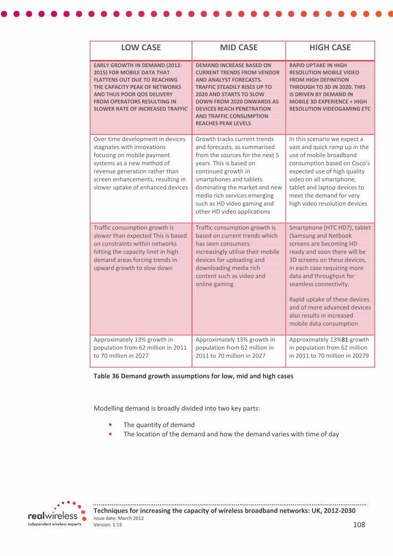
Techniques for increasing the capacity of wireless broadband networks: UK, 2012-2030 Issue date: March 2012
Version: 1.15 108
LOW CASE MID CASE HIGH CASE
EARLY GROWTH IN DEMAND (2012-
2015) FOR MOBILE DATA THAT
FLATTENS OUT DUE TO REACHING
THE CAPACITY PEAK OF NETWORKS
AND THUS POOR QOS DELIVERY
FROM OPERATORS RESULTING IN
SLOWER RATE OF INCREASED TRAFFIC
DEMAND INCREASE BASED ON
CURRENT TRENDS FROM VENDOR
AND ANALYST FORECASTS.
TRAFFIC STEADILY RISES UP TO
2020 AND STARTS TO SLOW
DOWN FROM 2020 ONWARDS AS
DEVICES REACH PENETRATION
AND TRAFFIC CONSUMPTION
REACHES PEAK LEVELS
RAPID UPTAKE IN HIGH
RESOLUTION MOBILE VIDEO
FROM HIGH DEFINITION
THROUGH TO 3D IN 2020. THIS
IS DRIVEN BY DEMAND IN
MOBILE 3D EXPERIENCE + HIGH
RESOLUTION VIDEOGAMING ETC
Over time development in devices
stagnates with innovations
focusing on mobile payment
systems as a new method of
revenue generation rather than
screen enhancements, resulting in
slower uptake of enhanced devices
Growth tracks current trends
and forecasts, as summarised
from the sources for the next 5
years. This is based on
continued growth in
smartphones and tablets
dominating the market and new
media rich services emerging
such as HD video gaming and
other HD video applications
In this scenario we expect a
vast and quick ramp up in the
use of mobile broadband
consumption based on Cisco’s
expected use of high quality
video on all smartphone,
tablet and laptop devices to
meet the demand for very
high video resolution devices
Traffic consumption growth is
slower than expected This is based
on constraints within networks
hitting the capacity limit in high
demand areas forcing trends in
upward growth to slow down
Traffic consumption growth is
based on current trends which
has seen consumers
increasingly utilise their mobile
devices for uploading and
downloading media rich
content such as video and
online gaming
Smartphone (HTC HD7), tablet
(Samsung and Netbook
screens are becoming HD
ready and soon there will be
3D screens on these devices,
in each case requiring more
data and throughput for
seamless connectivity.
Rapid uptake of these devices
and of more advanced devices
also results in increased
mobile data consumption
Approximately 13% growth in
population from 62 million in 2011
to 70 million in 2027
Approximately 13% growth in
population from 62 million in
2011 to 70 million in 2027
Approximately 13%81 growth
in population from 62 million
in 2011 to 70 million in 20279
Table 36 Demand growth assumptions for low, mid and high cases
Modelling demand is broadly divided into two key parts:
• The quantity of demand
• The location of the demand and how the demand varies with time of day

Techniques for increasing the capacity of wireless broadband networks: UK, 2012-2030 Issue date: March 2012
Version: 1.15 109
The amount of demand generated depends on a number of independent elements:
• Penetration of different devices types within the population such as:
• Smartphones, Tablets, Dongles etc.
• Multiple devices per user will result in >>100% penetration overall
• Traffic generated per device type (MB/month)
• E.g. laptops generate more traffic than smartphones per session
In this study we consider demand is generated by the following device types:
• Smartphones - These devices are considered to be high end handsets that utilise
both touchscreen and non-touchscreen interface and used for mobile data such
as video, audio, email etc. amongst other applications such as voice calls. Types
of Operating System found in these devices include Android, iOS, Symbian and
Windows etc. The volume of traffic generated by these devices is expected to be
a third of that generated by tablets.
• Tablets – These are considered mobile PC’s with large high resolution
touchscreens with the ability to surf the web, stream video, audio, basic editing
of documents, email etc. The volume of traffic generated by these devices is
expected to be a quarter that of embedded laptops
• Embedded laptops – Laptop PC’s with embedded cellular modules to connect via
3G (4G in future) to the internet. These devices are expected to generate the
largest amount of traffic out of all the devices
• USB modems – USB modems are very basic devices that are plugged into Laptops
or tablets whenever necessary to connect to the 3G(4G in future) network. The
volume of traffic generated by these devices is expected to be a less than half of
that generated by laptops.
• 3G phones – These handsets have some data capabilities such as send email,
browse the internet but not good for high resolution video, predominantly used
for voice. The volume of traffic generated by these devices is expected to be a
more than a twentieth of that generated by smartphones.
• M2M10 (machine to machine) – These devices are basic modules embedded in
another machine or device that consumes very little data at frequent intervals.
(Early devices consume 10’s of kbps)
Our study investigates how the location of demand varies according to certain times of day.
We have chosen three key times to investigate based on source data (described later in
section 5.3):
• Work time 9-10: When users are mostly indoors at business addresses
• Rush hour 5-6pm: When users are mostly outdoors on the move along road and
rail routes
• Evening 8-9pm: When users are mostly indoors at residential addresses
Figure 5-3 outlines the processes involved in profiling demand in this way.
10
M2M was considered a special case for demand and did not feature as part of the core modelled devices

Techniques for increasing the capacity of wireless broadband networks: UK, 2012-2030 Issue date: March 2012
Version: 1.15 110
Figure 5-3 High level demand profiling
Section 3.3 discussed the choice of study areas to be modelled to determine the quantity of
capacity required in each area based on the demand for that area. Figure 5-4 illustrates, at
a high level, how the demand points are mapped on to the study areas, in this case Central
London (Urban). Each demand point is represented by either a residential delivery address,
a business delivery address or a road/rail point in kilometres. The data is based on postcode
database which provides the total number of delivery addresses for the study area and the
Ordnance Survey provides the length of road and rail data for the study area.
Figure 5-4 Demand points mapped on to the Central London study area

Techniques for increasing the capacity of wireless broadband networks: UK, 2012-2030 Issue date: March 2012
Version: 1.15 111
5.3 Demand methodology and detailed assumptions
The following methodology presents a step by step process of how mobile traffic demand
has been derived according to the source data and implemented into the model based on
our assumptions.
The methodology used was a bottom-up approach using the required set of distributions to
calculate the average demand generated by devices according to the level of penetration of
each device within the UK population. The process set out below illustrates the logical
sequence of calculations undertaken to derive the average demand in Megabits per second
(Mbps) for each of the demand points in the study area. Table 37 below provides the
demand points by type according to each of the study areas and their locations, and what
each location represents.

Techniques for increasing the capacity of wireless broadband networks: UK, 2012-2030 Issue date: March 2012
Version: 1.15 112
Demand in Mbps per demand point
Demand
type
Study area Indoor Outdoor
per
residential
delivery
address
Urban London Home Outside home e.g. Garden,
balcony, street
Suburban London Home Outside home e.g. Garden,
balcony, street
Lincolnshire and
Berkshire
Home Outside home e.g. Garden,
balcony, street
per
business
delivery
address
Urban London Offices, shops etc. Outside business e.g. Street,
car park, site
Suburban London Offices, shops etc. Outside business e.g. Street,
car park, site
Lincolnshire and
Berkshire
Industry, small
shops/offices
Outside business e.g. Street,
car park, site
per km of
road/rail
Motorway Cars/buses Pedestrians (Set to 0 as no
pedestrians along motorway)
A road Cars/buses Pedestrians (Set to 0 as
pedestrians located outdoors
business and residential)
B road Cars/buses Pedestrians (Set to 0 as
pedestrians located outdoors
business and residential)
Railway Trains Pedestrians (Set to 0 as no
pedestrians along rail track)
Table 37 Types of demand and the locations where it is generated within the study area

Techniques for increasing the capacity of wireless broadband networks: UK, 2012-2030 Issue date: March 2012
Version: 1.15 113
5.3.1 Process for deriving demand per study area
We adopted the following process to determine the average demand per demand type
(residential/business delivery address and road/rail route)
1. Evaluate penetration of each device type (devices per pop) from 2012-2030
2. Calculate number of each device type in the study area = penetration (step
1) x population in the study area, for each study area.
3. Evaluate average demand (Bytes/month) per device type from 2012-2030
4. Calculate total traffic (Bytes/month) in study area by device type = number of devices
of each type (step 2) x traffic per device (step 3)
a) Validate total traffic in the study area (summed across all device types)
against UK wide forecast (e.g. PA) scaled to population of study area
5. Calculate traffic rate (bits/second) for the three different times of day, by device type =
Total Traffic (step 4) / proportion monthly traffic during the hour
a) Convert Bytes/month into Bytes/day
b) Scale by proportion of daily traffic in the hour for: rush hour, work time, evening
(Mbps)
6. Split the total traffic (by device) across different locations for the three times of day =
total traffic in the hour for that device (step 5) x proportion of traffic across locations
(for each device type)
a) Traffic will move from business addresses, to on the roads/rail, to at home.
Resulting in a work time, rush hour and evening time, respectively
b) This step inherently gives you the traffic split by device type at each location
7. Sum traffic across device types for each location and time of day (step 6)
8. Evaluate traffic per address or km of road/rail = total traffic by location (step 7) /
number of addresses or km per study area
9. Traffic split by clutter type = Traffic per address or km x percent of rural, suburban or
urban clutter type
10. Split traffic by location according to indoor and outdoor components = proportion of
indoor /outdoor traffic per location x total traffic per location (step 9)
11. Distribution of data amongst individuals = Plot distribution of users (%) against
distribution traffic (%) for each year to 2030
In each step we present the data used to derive the growth assumptions and traffic values
which in some cases used various analyst and vendor forecasts or reports. In other steps,
basic calculations were conducted in order to divide or multiply the traffic according to that
step in the process. The example output plots have used the Central London study area
under the mid case scenario.
Techniques for increasing the capacity of wireless broadband networks: UK, 2012-2030 Issue date: March 2012
Version: 1.15 114
5.3.2 Practical implementation of demand points (Peak-to-mean ratio)
The average demand is represented as Mbps across three busy hours which means the user
experience is spread evenly across a whole hour for access to the network. In practice
demand is not spread evenly over the period, so we introduced a peak to mean ratio for
each of the demand points to represent a more practical level of service for each user.
The peak to mean ratio was calculated as 1:20 by using the Urban London study area as a
calibration area (since it has the highest demand density) and ensuring that the model
results lead to networks which were close in scale to today’s mobile operator networks.
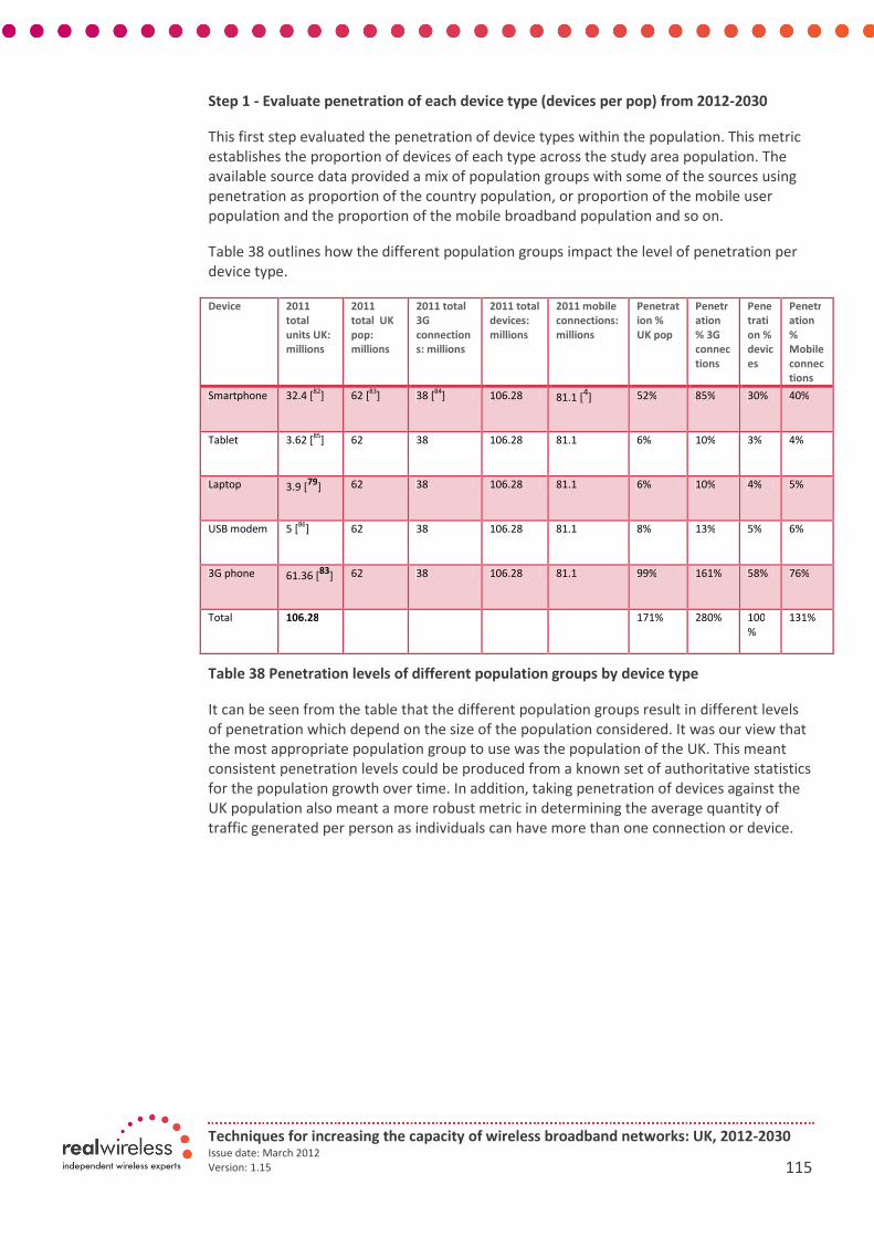
Techniques for increasing the capacity of wireless broadband networks: UK, 2012-2030 Issue date: March 2012
Version: 1.15 115
Step 1 - Evaluate penetration of each device type (devices per pop) from 2012-2030
This first step evaluated the penetration of device types within the population. This metric
establishes the proportion of devices of each type across the study area population. The
available source data provided a mix of population groups with some of the sources using
penetration as proportion of the country population, or proportion of the mobile user
population and the proportion of the mobile broadband population and so on.
Table 38 outlines how the different population groups impact the level of penetration per
device type.
Device 2011
total
units UK:
millions
2011
total UK
pop:
millions
2011 total
3G
connection
s: millions
2011 total
devices:
millions
2011 mobile
connections:
millions
Penetrat
ion %
UK pop
Penetr
ation
% 3G
connec
tions
Pene
trati
on %
devic
es
Penetr
ation
%
Mobile
connec
tions
Smartphone 32.4 [82
] 62 [83
] 38 [84
] 106.28 81.1 [4] 52% 85% 30% 40%
Tablet 3.62 [85
] 62 38 106.28 81.1 6% 10% 3% 4%
Laptop 3.9 [79
] 62 38 106.28 81.1 6% 10% 4% 5%
USB modem 5 [86
] 62 38 106.28 81.1 8% 13% 5% 6%
3G phone 61.36 [83
] 62 38 106.28 81.1 99% 161% 58% 76%
Total 106.28 171% 280% 100
%
131%
Table 38 Penetration levels of different population groups by device type
It can be seen from the table that the different population groups result in different levels
of penetration which depend on the size of the population considered. It was our view that
the most appropriate population group to use was the population of the UK. This meant
consistent penetration levels could be produced from a known set of authoritative statistics
for the population growth over time. In addition, taking penetration of devices against the
UK population also meant a more robust metric in determining the average quantity of
traffic generated per person as individuals can have more than one connection or device.
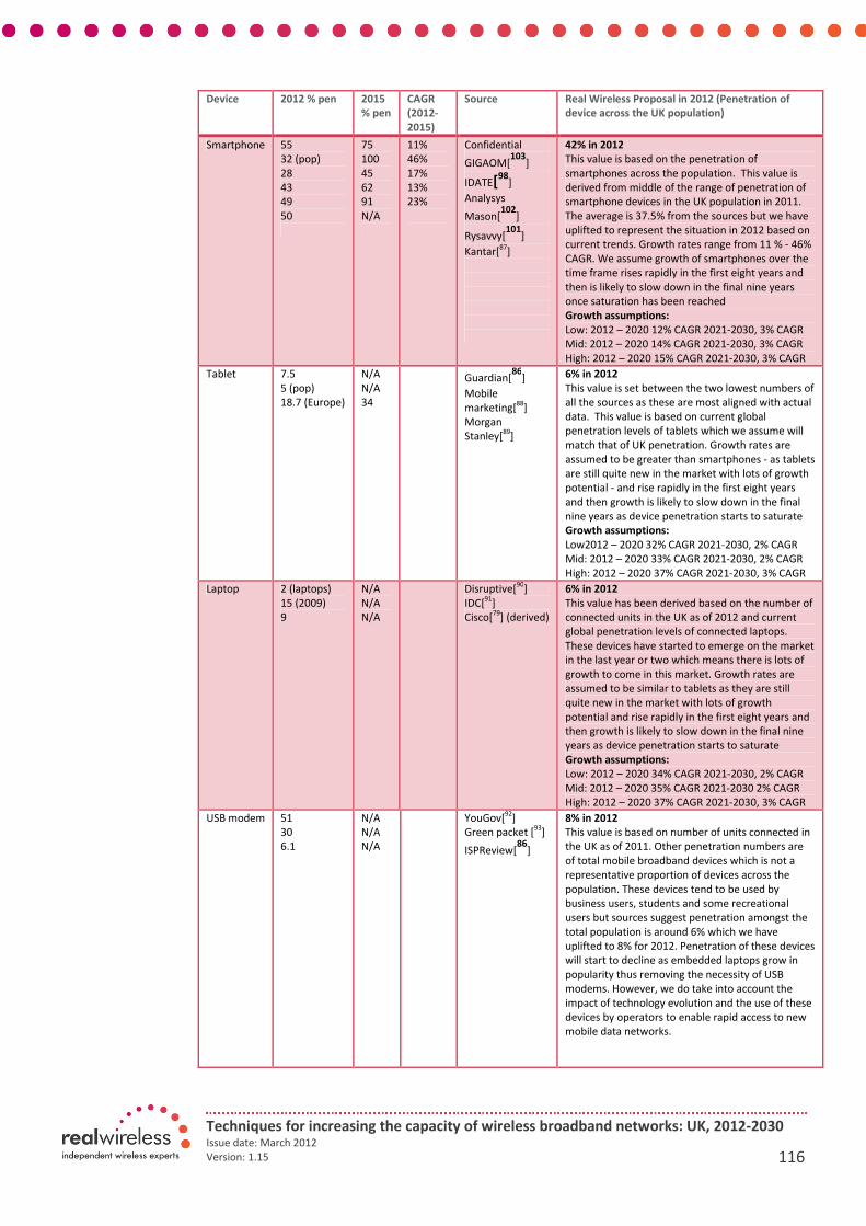
Techniques for increasing the capacity of wireless broadband networks: UK, 2012-2030 Issue date: March 2012
Version: 1.15 116
Device 2012 % pen 2015
% pen
CAGR
(2012-
2015)
Source Real Wireless Proposal in 2012 (Penetration of
device across the UK population)
Smartphone 55
32 (pop)
28
43
49
50
75
100
45
62
91
N/A
11%
46%
17%
13%
23%
Confidential
GIGAOM[103
]
IDATE[98
]
Analysys
Mason[102
]
Rysavvy[101
]
Kantar[87
]
42% in 2012
This value is based on the penetration of
smartphones across the population. This value is
derived from middle of the range of penetration of
smartphone devices in the UK population in 2011.
The average is 37.5% from the sources but we have
uplifted to represent the situation in 2012 based on
current trends. Growth rates range from 11 % - 46%
CAGR. We assume growth of smartphones over the
time frame rises rapidly in the first eight years and
then is likely to slow down in the final nine years
once saturation has been reached
Growth assumptions:
Low: 2012 – 2020 12% CAGR 2021-2030, 3% CAGR
Mid: 2012 – 2020 14% CAGR 2021-2030, 3% CAGR
High: 2012 – 2020 15% CAGR 2021-2030, 3% CAGR
Tablet 7.5
5 (pop)
18.7 (Europe)
N/A
N/A
34
Guardian[86
]
Mobile
marketing[88
]
Morgan
Stanley[89
]
6% in 2012
This value is set between the two lowest numbers of
all the sources as these are most aligned with actual
data. This value is based on current global
penetration levels of tablets which we assume will
match that of UK penetration. Growth rates are
assumed to be greater than smartphones - as tablets
are still quite new in the market with lots of growth
potential - and rise rapidly in the first eight years
and then growth is likely to slow down in the final
nine years as device penetration starts to saturate
Growth assumptions:
Low2012 – 2020 32% CAGR 2021-2030, 2% CAGR
Mid: 2012 – 2020 33% CAGR 2021-2030, 2% CAGR
High: 2012 – 2020 37% CAGR 2021-2030, 3% CAGR
Laptop 2 (laptops)
15 (2009)
9
N/A
N/A
N/A
Disruptive[90
]
IDC[91
]
Cisco[79
] (derived)
6% in 2012
This value has been derived based on the number of
connected units in the UK as of 2012 and current
global penetration levels of connected laptops.
These devices have started to emerge on the market
in the last year or two which means there is lots of
growth to come in this market. Growth rates are
assumed to be similar to tablets as they are still
quite new in the market with lots of growth
potential and rise rapidly in the first eight years and
then growth is likely to slow down in the final nine
years as device penetration starts to saturate
Growth assumptions:
Low: 2012 – 2020 34% CAGR 2021-2030, 2% CAGR
Mid: 2012 – 2020 35% CAGR 2021-2030 2% CAGR
High: 2012 – 2020 37% CAGR 2021-2030, 3% CAGR
USB modem 51
30
6.1
N/A
N/A
N/A
YouGov[92
]
Green packet [93
]
ISPReview[86
]
8% in 2012
This value is based on number of units connected in
the UK as of 2011. Other penetration numbers are
of total mobile broadband devices which is not a
representative proportion of devices across the
population. These devices tend to be used by
business users, students and some recreational
users but sources suggest penetration amongst the
total population is around 6% which we have
uplifted to 8% for 2012. Penetration of these devices
will start to decline as embedded laptops grow in
popularity thus removing the necessity of USB
modems. However, we do take into account the
impact of technology evolution and the use of these
devices by operators to enable rapid access to new
mobile data networks.

Techniques for increasing the capacity of wireless broadband networks: UK, 2012-2030 Issue date: March 2012
Version: 1.15 117
Growth assumptions:
Low: 2012 – 2020 2% CAGR 2021-2030, -14% CAGR
Mid: 2012 – 2020 1% CAGR 2021-2030, -12% CAGR
High: 2012 – 2020 5% CAGR 2021-2030, -2% CAGR
3G phone
77% (2010)
99%
64%
N/A
N/A
N/A
Incentivated[94
]
Mobile sqrd[82
]
Analysys
Mason[102
]
99% in 2012
This value is based on the number of expected early
3G type phones across the population in 2012.
Sources suggest there is almost 1 3G phone per pop.
These devices are likely to be replaced by
smartphones as new devices come on to the market.
In addition, vendors are now focusing produces on
smartphone technology and new sales of 3G phones
likely to decline
Growth assumptions:
Low: 2012 – 2020 -49% CAGR 2021-2030, -100%
CAGR
Mid: 2012 – 2020 -49% CAGR 2021-2030, -100%
CAGR
High: 2012 – 2020 -49% CAGR 2021-2030, -100%
CAGR
Table 39 Penetration of devices across the across various populations
Figure 5-5 Penetration of smartphones across mix of sources and Real Wireless proposal
Figure 5-5 compares the main sources for smartphones, since there were more sources for
this device compared to the other devices, against the Real Wireless proposal which is
within the middle of the range compared to the sources. The Real Wireless proposal sits
between the Analysys Mason forecast and the GIGAOM forecast which suggests a mid-
range between the relevant population forecasts.
0
20
40
60
80
100
120
2011 2012 2013 2014 2015 2016
% p
en
etr
ati
on
of
mix
po
pu
lati
on
gro
up
s
Penetration of smartphones across
different sources
confidential (Users)
GIGAOM (Pop)
IDATE (shipments)
Analysys Mason (Pop)
Rysavvy
Real Wireless

Techniques for increasing the capacity of wireless broadband networks: UK, 2012-2030 Issue date: March 2012
Version: 1.15 118
The following growth assumptions have been made for device penetration:
• Growth assumptions have been based on the sources for each of the device types
as closely aligned with public market data for 2011 and used for the starting point
in 2012
• Extending growth over a longer period but keeping the rate the same depending
on the high medium and low scenario
• The growth rates for smartphones are based on sources up to 2015
• The growth for tablets has been assumed to be slightly lower than smartphones
based on the higher tier consumer growth market for tablets
• The growth rates for laptops and USB dongles is based on sources which suggest
there will be parity between devices by 2015
• Growth in traffic for early 3G phones is based on source data with a steady
declining rate to 0% by 2025
The plots in Figure 5-6, Figure 5-7 and Figure 5-8 show the different rates of penetration
per device across the study time frame. The trend in each scenario is consistent in that:
• Smartphone penetration takes the highest proportion out of all devices
• Tablet and laptop penetration are the next two devices with the highest
penetration after smartphones
• USB modem (i.e. dongle) penetration does not grow but remains consistent over
much of the timeframe up to 2025 when the penetration begins to decrease
• 3G phones are already in decline from 2012 and continue to decline in
penetration until 2020 when they are no longer available

Techniques for increasing the capacity of wireless broadband networks: UK, 2012-2030 Issue date: March 2012
Version: 1.15 119
Figure 5-6 Device penetration for the low case scenario
Figure 5-7 Device penetration for the mid case scenario
Figure 5-8 Device penetration high case scenario
0%
50%
100%
150%
200%
250%
300%
350%
% d
ev
ice
pe
ne
tra
tio
n (
po
p)
Device penetration - Low case
3G phone
Dongles
Tablet
Laptop/Netbook
Smartphone
0%
50%
100%
150%
200%
250%
300%
350%
% d
ev
ice
pe
ne
tra
tio
n (
po
p)
Device penetration - Mid case
3G phone
Dongles
Tablet
Laptop/Netbook
Smartphone
0%
50%
100%
150%
200%
250%
300%
350%
400%
450%
% d
ev
ice
pe
ne
tra
tio
n (
po
p)
Device penetration - High case
3G phone
Dongles
Tablet
Laptop/Netbook
Smartphone
Low case:
• Decline in total
penetration owing
to 3G phone
decline with slow
growth of
smartphones,
tablets and
laptops
Mid case:
• Gradual growth
with devices
reaching 250% of
the population
across the device
mix
High case:
• Fast growth with
devices reaching
380% of the
population across
the device mix
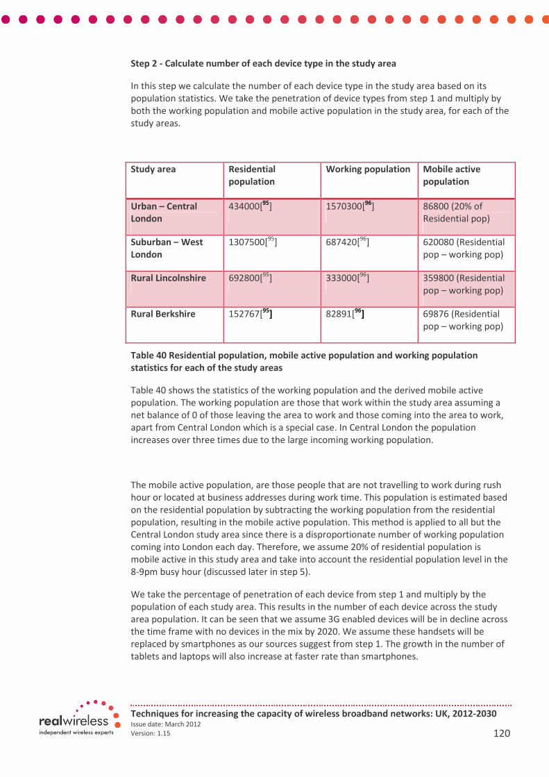
Techniques for increasing the capacity of wireless broadband networks: UK, 2012-2030 Issue date: March 2012
Version: 1.15 120
Step 2 - Calculate number of each device type in the study area
In this step we calculate the number of each device type in the study area based on its
population statistics. We take the penetration of device types from step 1 and multiply by
both the working population and mobile active population in the study area, for each of the
study areas.
Study area Residential
population
Working population Mobile active
population
Urban – Central
London
434000[95
] 1570300[96
] 86800 (20% of
Residential pop)
Suburban – West
London
1307500[95
] 687420[96
] 620080 (Residential
pop – working pop)
Rural Lincolnshire 692800[95
] 333000[96
] 359800 (Residential
pop – working pop)
Rural Berkshire 152767[95
] 82891[96
] 69876 (Residential
pop – working pop)
Table 40 Residential population, mobile active population and working population
statistics for each of the study areas
Table 40 shows the statistics of the working population and the derived mobile active
population. The working population are those that work within the study area assuming a
net balance of 0 of those leaving the area to work and those coming into the area to work,
apart from Central London which is a special case. In Central London the population
increases over three times due to the large incoming working population.
The mobile active population, are those people that are not travelling to work during rush
hour or located at business addresses during work time. This population is estimated based
on the residential population by subtracting the working population from the residential
population, resulting in the mobile active population. This method is applied to all but the
Central London study area since there is a disproportionate number of working population
coming into London each day. Therefore, we assume 20% of residential population is
mobile active in this study area and take into account the residential population level in the
8-9pm busy hour (discussed later in step 5).
We take the percentage of penetration of each device from step 1 and multiply by the
population of each study area. This results in the number of each device across the study
area population. It can be seen that we assume 3G enabled devices will be in decline across
the time frame with no devices in the mix by 2020. We assume these handsets will be
replaced by smartphones as our sources suggest from step 1. The growth in the number of
tablets and laptops will also increase at faster rate than smartphones.
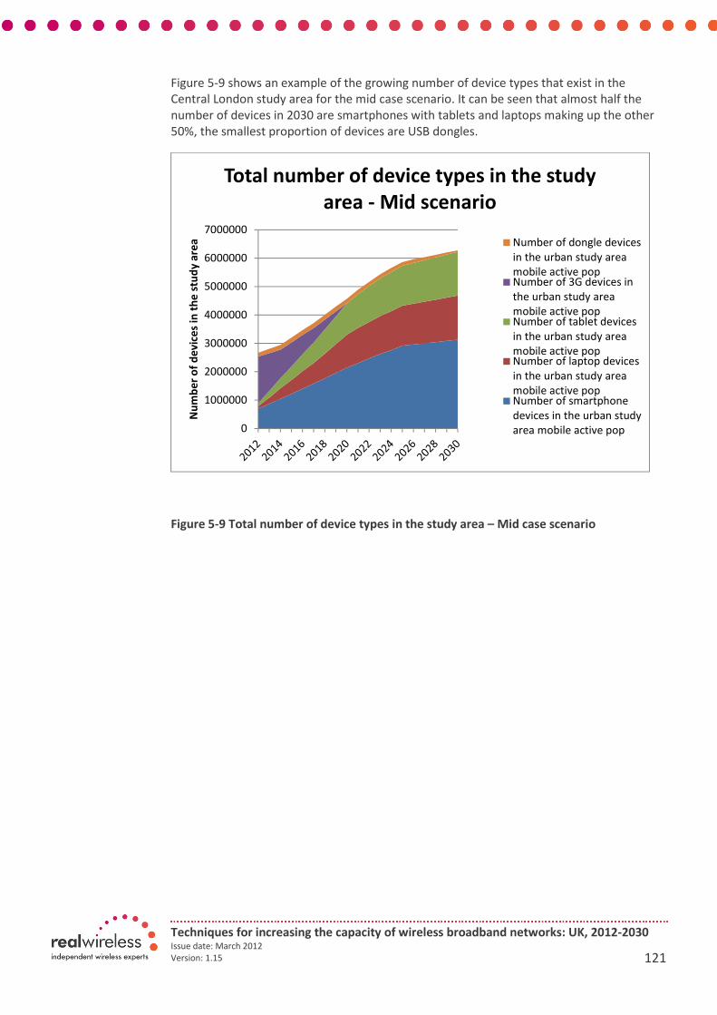
Techniques for increasing the capacity of wireless broadband networks: UK, 2012-2030 Issue date: March 2012
Version: 1.15 121
Figure 5-9 shows an example of the growing number of device types that exist in the
Central London study area for the mid case scenario. It can be seen that almost half the
number of devices in 2030 are smartphones with tablets and laptops making up the other
50%, the smallest proportion of devices are USB dongles.
Figure 5-9 Total number of device types in the study area – Mid case scenario
0
1000000
2000000
3000000
4000000
5000000
6000000
7000000
Nu
mb
er
of
de
vic
es
in t
he
stu
dy
are
a
Total number of device types in the study
area - Mid scenario
Number of dongle devices
in the urban study area
mobile active popNumber of 3G devices in
the urban study area
mobile active popNumber of tablet devices
in the urban study area
mobile active popNumber of laptop devices
in the urban study area
mobile active popNumber of smartphone
devices in the urban study
area mobile active pop
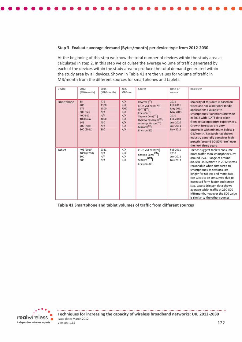
Techniques for increasing the capacity of wireless broadband networks: UK, 2012-2030 Issue date: March 2012
Version: 1.15 122
Step 3- Evaluate average demand (Bytes/month) per device type from 2012-2030
At the beginning of this step we know the total number of devices within the study area as
calculated in step 2. In this step we calculate the average volume of traffic generated by
each of the devices within the study area to produce the total demand generated within
the study area by all devices. Shown in Table 41 are the values for volume of traffic in
MB/month from the different sources for smartphones and tablets.
Device 2012
(MB/month)
2015
(MB/month)
2020
MB/mon
Source Date of
source
Real view
Smartphone 85
200
375
500 max
400-500
1000 max
146
600 (max)
300 (2011)
776
1300
1500
N/A
N/A
4000
450
N/A
800
N/A
N/A
7000
N/A
N/A
N/A
N/A
N/A
N/A
Informa [97
]
Cisco VNI 2011[79] IDATE[
98]
Ericsson[99
]
Sharma Cons[100
]
Rysavvy research[101
]
Analysys Mason[102
]
Gigaom[103
]
Ericsson[80]
2011
Feb 2011
May 2011
May 2011
2010
Feb 2010
July 2010
July 2011
Nov 2011
Majority of this data is based on
video and social network media
applications available to
smartphones. Variations are wide
in 2012 with IDATE data taken
from actual operators experiences.
Growth forecasts are very
uncertain with minimum below 1
GB/month. Research has shown
industry generally perceives high
growth (around 50-80% -YoY) over
the next three years
Tablet 405 (2010)
1000 (2010)
800
800
2311
N/A
N/A
N/A
N/A
N/A
N/A
N/A
Cisco VNI 2011[79]
Sharma Cons[100
]
Gigaom[103
]
Ericsson[80]
Feb 2011
2010
July 2011
Nov 2011
Trends suggest tablets consume
more traffic than smartphones, by
around 25%. Range of around
800MB -1GB/month in 2012 seems
reasonable when compared to
smartphones as sessions last
longer for tablets and more data
can Wireless be consumed due to
increased form factor and screen
size. Latest Ericsson data shows
average tablet traffic at 250-800
MB/month, however the 800 value
is similar to the other sources
Table 41 Smartphone and tablet volumes of traffic from different sources
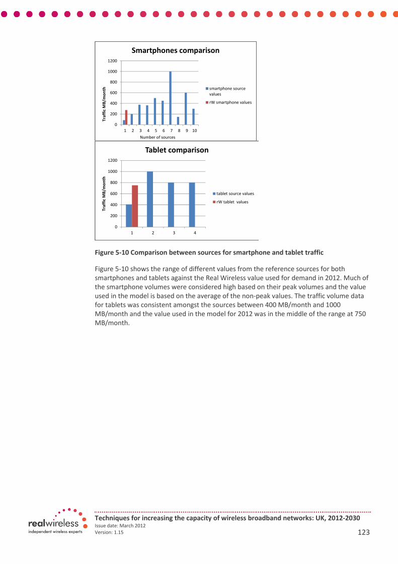
Techniques for increasing the capacity of wireless broadband networks: UK, 2012-2030 Issue date: March 2012
Version: 1.15 123
Figure 5-10 Comparison between sources for smartphone and tablet traffic
Figure 5-10 shows the range of different values from the reference sources for both
smartphones and tablets against the Real Wireless value used for demand in 2012. Much of
the smartphone volumes were considered high based on their peak volumes and the value
used in the model is based on the average of the non-peak values. The traffic volume data
for tablets was consistent amongst the sources between 400 MB/month and 1000
MB/month and the value used in the model for 2012 was in the middle of the range at 750
MB/month.
0
200
400
600
800
1000
1200
1 2 3 4 5 6 7 8 9 10
Tra
ffic
MB
/mo
nth
Smartphones comparison
smartphone source
values
rW smartphone values
Number of sources
0
200
400
600
800
1000
1200
1 2 3 4
Tra
ffic
MB
/mo
nth
Tablet comparison
tablet source values
rW tablet values
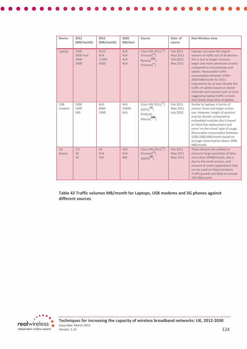
Techniques for increasing the capacity of wireless broadband networks: UK, 2012-2030 Issue date: March 2012
Version: 1.15 124
Device 2012
(MB/month)
2015
(MB/month)
2020
MB/mon
Source Date of
source
Real Wireless view
Laptop 2500
5000 max
3500
1900
6522
N/A
11200
6500
N/A
N/A
N/A
N/A
Cisco VNI 2011[79
]
Ericsson[80
]
Rysavy[101
]
Ericsson[80
]
Feb 2011
May 2011
Feb 2010
Nov 2011
Laptops consume the largest
volume of traffic out of all devices -
this is due to longer sessions,
larger and more advanced screens
compared to smartphones and
tablets. Reasonable traffic
consumption between 2500 –
3000 MB/month for 2012.
Expected to be at least double the
traffic of tablets based on above
rationale and sources such as Cisco
suggesting laptop traffic is more
than three times that of tablets.
USB
modem
2000
1000
500
N/A
8000
1969
N/A
15000
N/A
Cisco VNI 2011[79
]
IDATE[98
]
Analysys
Mason[102
]
Feb 2011
May 2011
July 2010
Similar to laptops in terms of
session times and larger screen
use. However, length of sessions
may be shorter compared to
embedded modules this is based
on fixed line replacement and
more ‘on the move’ type of usage.
Reasonable consumption between
1500-2000 MB/month based on
average consumption above 1000
MB/month
3G
phone
3.3
50
50
54
N/A
500
N/A
N/A
800
Cisco VNI 2011[79
]
Ericsson[80
]
IDATE[98
]
Feb 2011
May 2011
May 2011
These devices are unlikely to
consume large quantities of data
more than 50MB/month, this is
due to the small screens, and
amount of useful applications that
can be used on these handsets.
Traffic growth not likely to exceed
100 MB/month
Table 42 Traffic volumes MB/month for Laptops, USB modems and 3G phones against
different sources

Techniques for increasing the capacity of wireless broadband networks: UK, 2012-2030 Issue date: March 2012
Version: 1.15 125
Figure 5-11 Comparison between sources for smartphone and tablet traffic
Figure 5-11 shows the range of different values from the reference sources for both laptops
and USB modems against the Real Wireless value used for demand in 2012. Laptop traffic
varied quite widely amongst the sources and we took the average of the non-peak traffic
data as the level in 2012. The Real Wireless value for USB modems was based on the
average of all the source numbers, as data available for mobile broadband traffic across
modems is aligned with traffic volumes measured in practice around 1100 MB/month on
average.
Traffic demand of devices
• The multiple sources as shown in Table 41 and Table 42 provide a wide range of
traffic values per device. We used the average excluding the maximum of those
numbers as the value in 2012
Growth assumptions:
• Growth assumptions have been broadly based on the sources for each of the
device types aligned with public market data for 2011 and the average used for
the starting point in 2012 for each device (except 3G phones)
• We have assumed extended growth trends over a longer period (8-10 years)
keeping the rate the same depending on the high medium and low scenarios
• We assumed the rate of growth in the latter part of the time frame would fall
based on the maturity of the market and that consumption of applications will
reach a certain limit based on patterns of mobile use over time[104].
• The growth rates for tablets and laptops are considered to be similar owing to
similar trends in data consumption across those devices. This includes, video
streaming, audio streaming, email and download of high resolution content
0
2000
4000
6000
1 2 3 4
Tra
ffic
MB
/mo
nth
Laptop comparison
laptop source
values
rW laptop values
Number of sources
0
1000
2000
3000
1 2 3 4
Tra
ffic
MB
/mo
nth
USB comparison
USB source
values
rW USB values
Number of sources

Techniques for increasing the capacity of wireless broadband networks: UK, 2012-2030 Issue date: March 2012
Version: 1.15 126
• The growth rates for USB dongles begin to decline in the latter years of the
timeframe due to the uptake of embedded laptops. We expect laptops to start
taking the share of the dongle traffic as more embedded laptops become
available on the market.
• Growth in traffic for 3G phones is based on the IDATE source which provides data
up to 2020. This shows that in 2020 there will still be 3G enabled handsets in
2020. Our assumption suggests these handsets will be superseded by
smartphones and future generations of smartphones, although we assume the
traffic will grow on the 3G handsets until they are phased out.
Device Traffic in 2012 Year Low CAGR Mid CAGR High
CAGR
Smartphone 270 MB/month 2012-2020 4% 10% 20%
2021-2030 4% 8% 12%
Tablet 751 MB/month 2012-2020 6% 15% 25%
2021-2030 6% 13% 17%
Laptop 2633 MB/month 2012-2020 6% 15% 25%
2021-2030 6% 12% 17%
USB 1125 MB/month 2012-2020 5% 13% 18%
2021-2030 1% 4% 8%
3G phone 10 MB/month 2012-2020 5% 11% 14%
2021-2030 0% 0% 0%
Table 43 Mobile traffic growth assumptions
Table 43 shows the traffic growth rates we have assumed across each of the devices for the
low, mid and high scenarios. The figures suggest the highest rate of growth will come from
tablets and laptops which aligns with sources such as Cisco[79
] and Ericsson[80
]. However,
smartphone traffic will also continue to rapidly grow over the next five years which is
considered under our mid/high scenarios whose range is closest to Analysys Mason[102
] of

Techniques for increasing the capacity of wireless broadband networks: UK, 2012-2030 Issue date: March 2012
Version: 1.15 127
48% CAGR rather than higher estimates from Cisco[79] 119% CAGR Rysavy Research[101
]
and Ericsson[80
] 60% CAGR.
USB modem traffic is still likely to grow over the study timeframe as mobile broadband
evolves into new technologies and dongles offer a ‘quick to market’ solution for operators
to switch users on to new networks. However, growth will likely be lower than tablet and
laptop traffic and more than smartphone traffic based on the ‘shorter session’ use of USB
modems compared to tablets and embedded laptops.
Figure 5-12 shows the growth of traffic in GB/month per device over time according to the
mid-scenario. Laptop traffic is clearly the device which is likely to consume the most traffic
in future, followed by tablets, then USB modems and then smartphones.
The output suggests that laptop traffic will generate almost traffic, almost 25 GB/month by
2030 with tablets the next highest traffic consuming device at 8 GB/month on average and
UB dongles on 5 GB/month. We estimate smartphones, in this case, will generate around
1.3 GB/month on average by 2030.
Figure 5-12 Mobile traffic growth across devices – Mid scenario
Step 4 - Calculate total traffic (Bytes/month) in study area by device type
In this step we calculate total traffic in the study area by device type. This means the ‘total
quantity’ of traffic for the study area, which has been based on the population (working and
0.00
5.00
10.00
15.00
20.00
25.00
2010 2015 2020 2025 2030
Tra
ffic
GB
/mo
nth
Year
Mobile traffic growth across devices -
Mid scenarioAvg amount of demand
from an urban suburban
user laptop (GB/month)
Avg amount of demand
from an urban and
suburban user tablet
(GB/month)
Avg amount of demand
from an urban suburban
user dongle (GB/month)
Avg amount of demand
from an urban and
suburban user
smartphone (GB/month)
Avg amount of demand
from an urban suburban
user 3G phone
(GB/month)

Techniques for increasing the capacity of wireless broadband networks: UK, 2012-2030 Issue date: March 2012
Version: 1.15 128
mobile active) of the study area and penetration of devices, can be distributed across the
study area locations and times of day to calculate the average demand per demand point.
In this step we take the number of devices of each type from step 2 and multiply the traffic
per device from step 3.
Figure 5-13 shows an example of the total mobile traffic generated in the Central London
study area for the mid scenario across device types. The largest proportion of traffic
generated is from laptops taking over 60% of the total traffic followed by tablets and then
smartphones. USB dongles and 3G phones become a very low proportion of the total traffic
in this case.
Figure 5-13 Total mobile traffic in the Central London urban study area by device type –
Mid scenario
We expect the Central London study area to generate the highest amount of traffic across
all the study areas due to having the largest population and we can compare the total
mobile traffic in 2030 in Figure 5-13 against the total mobile traffic in Figure 5-14 which is
the Lincolnshire rural study area which shows a factor of 6 difference between the two
study areas.
0
500000
1000000
1500000
2000000
2500000
3000000
Tra
ffic
GB
/mo
nth
Total traffic in the study area by device type
- Mid scenario
Amount of total traffic from
dongle users in the study area
total pop(GB/month)
Amount of total traffic from 3G
users users in the study area
total pop(GB/month)
Amount of total traffic from
tablet users in the study area
total(GB/month)
Amount of total traffic from
laptop users in the study area
total pop (GB/month)
Amount of avg traffic from
smartphone users in the study
area total pop (GB/month)
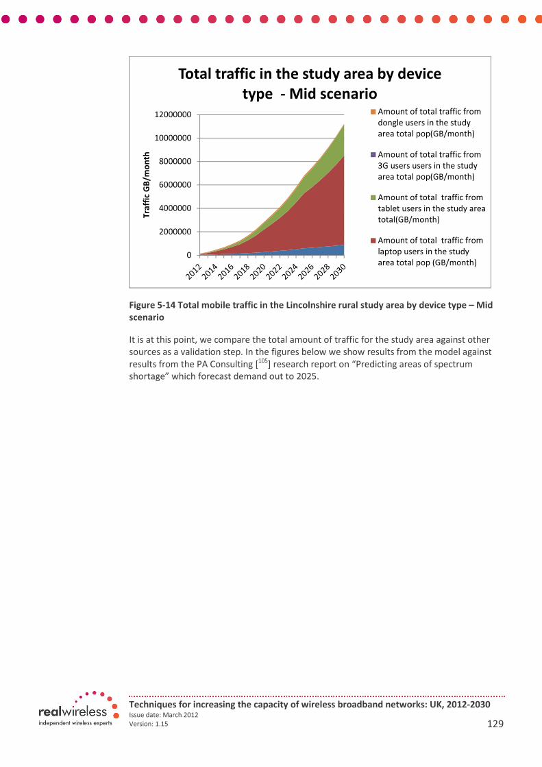
Techniques for increasing the capacity of wireless broadband networks: UK, 2012-2030 Issue date: March 2012
Version: 1.15 129
Figure 5-14 Total mobile traffic in the Lincolnshire rural study area by device type – Mid
scenario
It is at this point, we compare the total amount of traffic for the study area against other
sources as a validation step. In the figures below we show results from the model against
results from the PA Consulting [105
] research report on “Predicting areas of spectrum
shortage” which forecast demand out to 2025.
0
2000000
4000000
6000000
8000000
10000000
12000000
Tra
ffic
GB
/mo
nth
Total traffic in the study area by device
type - Mid scenarioAmount of total traffic from
dongle users in the study
area total pop(GB/month)
Amount of total traffic from
3G users users in the study
area total pop(GB/month)
Amount of total traffic from
tablet users in the study area
total(GB/month)
Amount of total traffic from
laptop users in the study
area total pop (GB/month)
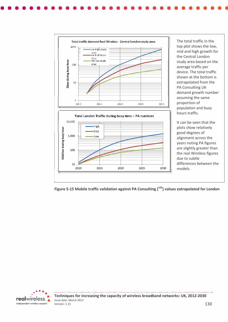
Techniques for increasing the capacity of wireless broadband networks: UK, 2012-2030 Issue date: March 2012
Version: 1.15 130
Figure 5-15 Mobile traffic validation against PA Consulting [105
] values extrapolated for London
The total traffic in the
top plot shows the low,
mid and high growth for
the Central London
study area based on the
average traffic per
device. The total traffic
shown at the bottom is
extrapolated from the
PA Consulting UK
demand growth number
assuming the same
proportion of
population and busy
hours traffic.
It can be seen that the
plots show relatively
good degrees of
alignment across the
years noting PA figures
are slightly greater than
the real Wireless figures
due to subtle
differences between the
models.

Techniques for increasing the capacity of wireless broadband networks: UK, 2012-2030 Issue date: March 2012
Version: 1.15 131
Figure 5-16 Traffic validation against PA Consulting forecast for all of UK
Figure 5-16 shows another comparison chart between Real Wireless growth estimates
against PA Consulting forecasts for demand growth for the whole UK. The Real Wireless
figures used the latest UK population estimates for 2011[83
] and the penetration values and
traffic volume per device estimates to produce the Real Wireless curves in the plot above. It
can be seen that the starting point in 2012 is just below the PA mid curve for 2012 which
suggests good correlation between the data. The growth curves differ in that our estimates,
based on average traffic volume per device, show a rapid increase in the early years in all
scenarios which means our low case scenario closely follows the PA-mid case, however the
rate of growth shows good correlation.
All our scenario cases lie between PA mid and high cases with our high case starting to
increase above the PA high around 2015. This suggests that our estimates are within
plausible ranges of independent forecasts.
1
10
100
1000
10000
2010 2015 2020 2025 2030
PB
/mo
nth
Real Wireless UK demand vs. PA forecast UK
rW high
PA High
rW mid
PA Mid
rW low
PA Low
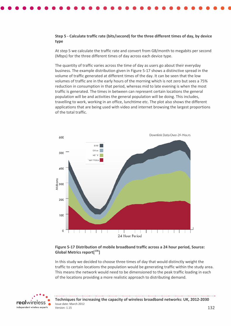
Techniques for increasing the capacity of wireless broadband networks: UK, 2012-2030 Issue date: March 2012
Version: 1.15 132
Step 5 - Calculate traffic rate (bits/second) for the three different times of day, by device
type
At step 5 we calculate the traffic rate and convert from GB/month to megabits per second
(Mbps) for the three different times of day across each device type.
The quantity of traffic varies across the time of day as users go about their everyday
business. The example distribution given in Figure 5-17 shows a distinctive spread in the
volume of traffic generated at different times of the day. It can be seen that the low
volumes of traffic are in the early hours of the morning which is not zero but sees a 75%
reduction in consumption in that period, whereas mid to late evening is when the most
traffic is generated. The times in between can represent certain locations the general
population will be and activities the general population will be doing. This includes,
travelling to work, working in an office, lunchtime etc. The plot also shows the different
applications that are being used with video and internet browsing the largest proportions
of the total traffic.
Figure 5-17 Distribution of mobile broadband traffic across a 24 hour period, Source:
Global Metrics report[106
]
In this study we decided to choose three times of day that would distinctly weight the
traffic to certain locations the population would be generating traffic within the study area.
This means the network would need to be dimensioned to the peak traffic loading in each
of the locations providing a more realistic approach to distributing demand.

Techniques for increasing the capacity of wireless broadband networks: UK, 2012-2030 Issue date: March 2012
Version: 1.15 133
Figure 5-18 relative traffic volume according to locations across a 24 hour period, Source:
Nokia Siemens[107
]
Figure 5-18 shows the relative traffic for the various locations across a 24 hour period which
we based our assumptions for dividing traffic across the three times of day. The plot in the
figure shows the mix of City, suburban and residential area traffic, varying according to the
time of day. Traffic progressively grows in the suburbs throughout the day, however this is
exceeded by traffic in the City location as the population arrives at work. The residential
traffic matches the suburbs from around 6pm onwards to 12am and City traffic is in decline
from 3pm onwards.
Similar to the plot in Figure 5-17 the period of lowest consumption occurs in the late
evening and early morning hours across all locations types.
Figure 5-19 Real Wireless proposal for traffic across three different times of day, Source:
Elisa[108]
and Nokia-Siemens[107
]

Techniques for increasing the capacity of wireless broadband networks: UK, 2012-2030 Issue date: March 2012
Version: 1.15 134
Our proposal for the three different busy hours per day is as follows:
a) 9-10am: At this hour of day we assume the majority of the traffic in each study area
will be generated from business locations
b) 5-6pm: At this hour of day we assume the majority of the traffic in each study area
will be generated by commuters either on the road (in-vehicle) or on trains along rail
lines
c) 8-9pm: At this hour of the day we assume the majority of the traffic in each study
area will be generated at residential locations
Figure 5-19 describes how we derived the proportion of traffic in each busy hour across the
total traffic in a 24 hour period from the distribution in the Elisa chart. This chart provides
the total quantity of traffic in each hour with details of the particular application. It also
broadly supports the trend found from the other distributions of how much traffic is
consumed at specific times of day.
Figure 5-20 Total mobile traffic across devices for three busy times of day
Figure 5-20 shows the output from the demand model of the total mobile traffic across
each of the three busy hours in the Central London study area.
0
100000
200000
300000
400000
500000
600000
700000
2012 2014 2016 2018 2020 2022 2024 2026 2028 2030
Mo
bil
e t
raff
ic (
Mb
ps)
Mobile traffic divided into three times of
day across devices
Total traffic across
devices 8-9pm
Total traffic across
devices 5-6pm
Total traffic across
devices 9-10am

Techniques for increasing the capacity of wireless broadband networks: UK, 2012-2030 Issue date: March 2012
Version: 1.15 135
Step 6 - Split the total traffic (by device) across different locations for the three times of
day
In this step we split the total traffic by device type for the three times of day calculated
from step 5 across the different locations within the study area. It is at this point we
determine the proportion of traffic across locations for each time of day and assume:
• Traffic will move from business addresses, to on the roads to at home. Resulting
in a work time, rush hour and evening time, respectively
• This step inherently gives you the traffic split by device type at each location
Figure 5-21 shows how the mobile active population and the working population are
distributed across locations for the different times of day. We have assumed that the
largest proportion of traffic should be distributed according to where largest proportion of
the population will be located. For example, the majority of the working population will be
at business locations between 9-10am; we assumed this to be 78% of the working
population and hence traffic. The other 22% of the traffic is ranked and distributed amongst
the other locations according to the next likely highest location which in this case is rail
(7%), residential (5%), Motorway (4%), A-road (4%), B-road (2%). The equivalent process is
done for the mobile active population, however, this population are more likely to be at
residential locations or road and rail locations and not business locations.
Figure 5-21 Traffic split by population both for mobile active and working populations

Techniques for increasing the capacity of wireless broadband networks: UK, 2012-2030 Issue date: March 2012
Version: 1.15 136
The following sets of figures provide extracts from the demand model of how the traffic is
split by device type for each of the locations for each time of day. The example shown in
the figures is for the Central London urban study area mid case scenario. Note the values of
mobile traffic at each of the locations for the different times which will impact the level of
capacity required.
Figure 5-22 Traffic at residential locations by device type for each of three busy hours
Figure 5-23 Traffic at business locations by device type for each of three busy hours
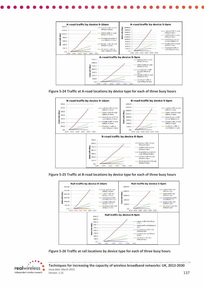
Techniques for increasing the capacity of wireless broadband networks: UK, 2012-2030 Issue date: March 2012
Version: 1.15 137
Figure 5-24 Traffic at A-road locations by device type for each of three busy hours
Figure 5-25 Traffic at B-road locations by device type for each of three busy hours
Figure 5-26 Traffic at rail locations by device type for each of three busy hours
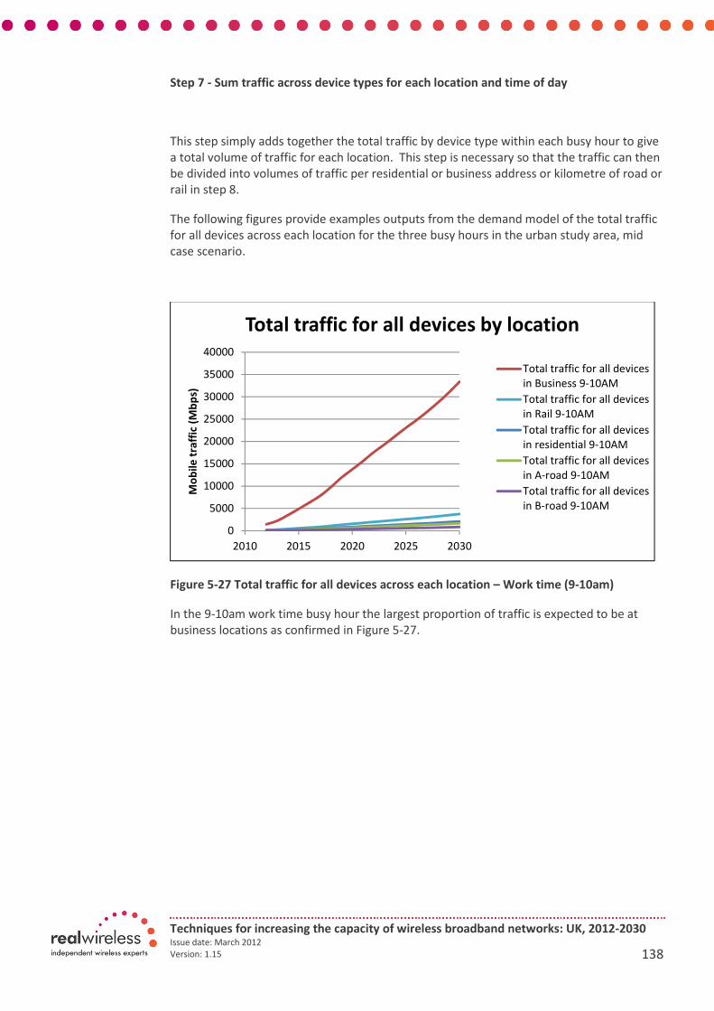
Techniques for increasing the capacity of wireless broadband networks: UK, 2012-2030 Issue date: March 2012
Version: 1.15 138
Step 7 - Sum traffic across device types for each location and time of day
This step simply adds together the total traffic by device type within each busy hour to give
a total volume of traffic for each location. This step is necessary so that the traffic can then
be divided into volumes of traffic per residential or business address or kilometre of road or
rail in step 8.
The following figures provide examples outputs from the demand model of the total traffic
for all devices across each location for the three busy hours in the urban study area, mid
case scenario.
Figure 5-27 Total traffic for all devices across each location – Work time (9-10am)
In the 9-10am work time busy hour the largest proportion of traffic is expected to be at
business locations as confirmed in Figure 5-27.
0
5000
10000
15000
20000
25000
30000
35000
40000
2010 2015 2020 2025 2030
Mo
bil
e t
raff
ic (
Mb
ps)
Total traffic for all devices by location
Total traffic for all devices
in Business 9-10AM
Total traffic for all devices
in Rail 9-10AM
Total traffic for all devices
in residential 9-10AM
Total traffic for all devices
in A-road 9-10AM
Total traffic for all devices
in B-road 9-10AM

Techniques for increasing the capacity of wireless broadband networks: UK, 2012-2030 Issue date: March 2012
Version: 1.15 139
Figure 5-28 Total traffic for all devices across each location – Rush hour time (5-6pm)
In the 5-6pm rush hour busy time the largest proportion of traffic is expected to be at the
road and rail locations as confirmed in Figure 5-28.
Figure 5-29 Total traffic for all devices across each location – Evening time (8-9pm)
In the 8-9pm rush hour busy time the largest proportion of traffic is expected to be at
residential locations as confirmed in Figure 5-29.
0
5000
10000
15000
20000
25000
30000
35000
2010 2015 2020 2025 2030
Mo
bil
e t
raff
ic (
Mb
ps)
Total traffic for all devices by location
Total traffic for all devices
in Rail 5-6PM
Total traffic for all devices
in A-road 5-6PM
Total traffic for all devices
in B-road 5-6PM
Total traffic for all devices
in residential 5-6PM
Total traffic for all devices
in Business 5-6PM
0
10000
20000
30000
40000
50000
60000
70000
80000
2010 2015 2020 2025 2030
Mo
bil
e t
raff
ic (
Mb
ps)
Total traffic for all devices by location
Total traffic for all devices
in residential 8-9PM
Total traffic for all devices
in Rail 8-9PM
Total traffic for all devices
in A-road 8-9PM
Total traffic for all devices
in Business 8-9PM
Total traffic for all devices
in B-road 8-9PM

Techniques for increasing the capacity of wireless broadband networks: UK, 2012-2030 Issue date: March 2012
Version: 1.15 140
Step 8 - Evaluate traffic per address or km of road/rail
This step takes the statistics for each of the study areas to calculate the average traffic in
Mbps per address of kilometre of road or rail. This step is necessary so that the traffic can
then be split according to its indoor or outdoor locations in the next step.
The statistics for each study can be seen in the tables below. The delivery address data has
been sourced from the UK postcode database and the road and rail data has been sourced
from the Ordnance Survey database.
Total delivery
addresses
Study area
Urban Suburban Rural Urban Suburban Rural
RESIDENTIAL BUSINESS
273,723 21,085 8,356 31,794 4,420 1,204 Urban Central
London Total 303,164 Total 37,418
Suburban
West London
40,090 395,298 38,877 3,212 18,600 2,104
Total 474,265 Total 23,916
Rural
Lincolnshire
22,484 192,163 114,964 806 9,097 6,196
Total 329,611 Total 16,099
Rural
Berkshire
643 46,585 23,704 15 2,654 1,259
Total 70,932 Total 3,928
Table 44 Absolute number of residential and business delivery addresses for each study
area
Study area Road/Rail (km)
Motorway A road B road Railway
Urban Central
London - 108 29 10
Suburban West
London 22 298 73 134
Rural Lincolnshire - 1,104 782 337
Rural Berkshire 45 128 74 56
Table 45 Absolute number of road and rail kilometres for each study area
The total number of delivery addresses for residential and business in each study area is
used to calculate total traffic per address for the study area. Similarly, the sum total of
kilometres for Motorway, A-road, B-road and rail in each study area is used to calculate
total traffic per address for the study area. Note there is 0 km of motorway in the urban
Central London and rural Lincolnshire study areas.

Techniques for increasing the capacity of wireless broadband networks: UK, 2012-2030 Issue date: March 2012
Version: 1.15 141
The following figures give examples of the quantity of demand for each busy hour at each
location within the Central London study area. The charts show the proportion of traffic per
delivery address, or per kilometre of road/rail according to the busy hour. It can be seen
that the mobile traffic generated on the road and rail is significant due to the smaller
quantities of kilometres compared to the much larger quantities of delivery addresses. This
means there is more traffic per kilometre for road/rail than for per residential or business
delivery addresses.
Figure 5-30 Total traffic per address or km by location in the 9-10am busy hour for Central London
Figure 5-31 Total traffic per address or km by location in the 5-6pm busy hour for Central
London
0
5
10
15
20
25
30
35
20
12
20
13
20
14
20
15
20
16
20
17
20
18
20
19
20
20
20
21
20
22
20
23
20
24
20
25
20
26
20
27
20
28
20
29
20
30
Mo
bil
e t
raff
ic (
Mb
ps)
Total traffic per address or km by location 9-10am
Total amount of traffic for rail per km
(Mbps)
Total amount of traffic for B-road per
km (Mbps)
Total amount of traffic for A-road per
km (Mbps)
Total amount of traffic for all devices
residential per address (Mbps)
Total amount of traffic for all devices
business per address (Mbps)
0
50
100
150
200
250
300
350
400
20
12
20
13
20
14
20
15
20
16
20
17
20
18
20
19
20
20
20
21
20
22
20
23
20
24
20
25
20
26
20
27
20
28
20
29
20
30
Mo
bil
e t
raff
ic (
Mb
ps)
Total traffic per address or km by location 5-6pm
Total amount of traffic for rail per km
(Mbps)
Total amount of traffic for B-road per
km (Mbps)
Total amount of traffic for A-road per
km (Mbps)
Total amount of traffic for all devices
residential per address (Mbps)
Total amount of traffic for all devices
business per address (Mbps)
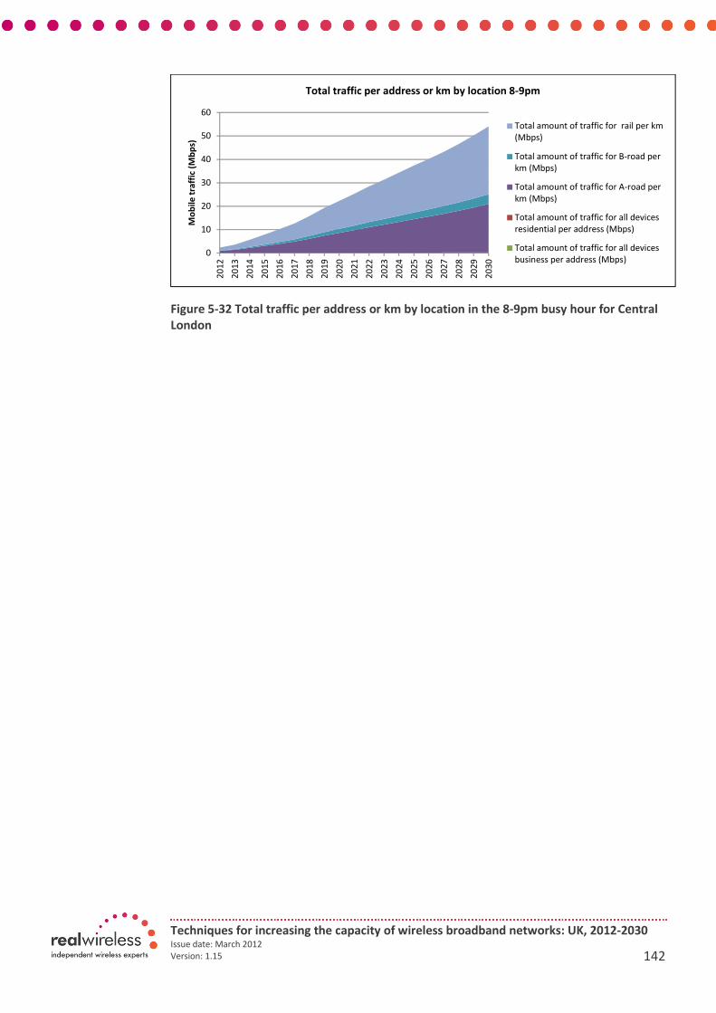
Techniques for increasing the capacity of wireless broadband networks: UK, 2012-2030 Issue date: March 2012
Version: 1.15 142
Figure 5-32 Total traffic per address or km by location in the 8-9pm busy hour for Central
London
0
10
20
30
40
50
60
20
12
20
13
20
14
20
15
20
16
20
17
20
18
20
19
20
20
20
21
20
22
20
23
20
24
20
25
20
26
20
27
20
28
20
29
20
30
Mo
bil
e t
raff
ic (
Mb
ps)
Total traffic per address or km by location 8-9pm
Total amount of traffic for rail per km
(Mbps)
Total amount of traffic for B-road per
km (Mbps)
Total amount of traffic for A-road per
km (Mbps)
Total amount of traffic for all devices
residential per address (Mbps)
Total amount of traffic for all devices
business per address (Mbps)
Techniques for increasing the capacity of wireless broadband networks: UK, 2012-2030 Issue date: March 2012
Version: 1.15 143
Step 9 – Traffic split by clutter type
In this step we split the traffic in the study area by clutter type. This has the impact of
distributing the traffic to the areas in which our demand points are located. The set of
assumptions made for this step are based on the location of devices expected in certain
clutter types taking into consideration our interpretation of clutter type.
An example definition of clutter types is given below extracted from “Antennas and
Propagation for Wireless communications Systems” [109, pp 167]:
• Open area: Open space, no tall trees or buildings in path, plot of land
cleared for 300–400 m ahead, e.g. farmland, rice fields, open fields.
• Suburban area: Village or highway scattered with trees and houses,
some obstacles near the mobile but not very congested.
• Urban area: Built up city or large town with large buildings and
houses with two or more storeys, or larger villages with close houses
and tall, thickly grown trees.
Assumptions:
We assume the average traffic per address and per km are equal for urban and suburban
clutter types, this is based on:
• We assume the total traffic generated by individuals within residential and
business locations for urban and suburban clutter types to be equal due to similar
proportions of devices within homes and offices and usage of devices is unlikely
to change
We assume the average traffic per address and per km for rural clutter type will be reduced
compared to urban and suburban clutter types, this is based on:
• We expect in rural clutter such as parks and open spaces the traffic will be greatly
reduced by a factor of almost 100 compared to urban and suburban clutter types
• We note these values will vary according to the study areas
Values:
• Urban and Suburban - 99% of total devices located in urban and suburban clutter
types
• Rural - 1% of devices located in urban and suburban clutter types
The above values are based on Ericsson’s traffic forecast[80
] for traffic generation reducing
across different clutter types which shows a declining proportion of traffic for rural areas
>30% in 2011 reducing to 16% in 2016. The value has then been adjusted according to the
expected quantity of devices found in rural clutter types such as open spaces, farm land etc,
which is assumed to be nearer 1% of devices in the study areas.

Techniques for increasing the capacity of wireless broadband networks: UK, 2012-2030 Issue date: March 2012
Version: 1.15 144
Calculation:
• Total traffic for residential/business address urban/suburban clutter type = 0.99 x
Total traffic per residential/business address (Mbps) (Step 8)
• Total traffic for residential/business address rural clutter type = 0.01 x Total
traffic per residential/business address (Mbps) (Step 8)

Techniques for increasing the capacity of wireless broadband networks: UK, 2012-2030 Issue date: March 2012
Version: 1.15 145
Step 10 - Split traffic by location according to indoor and outdoor components
It is in this step that traffic generated per address or kilometre is split according to the
indoor and outdoor components. This is an important step when dimensioning for traffic
since a lot of mobile traffic is offloaded when indoors and therefore the proportion of
traffic generated indoors can have an overall impact on the demand of cellular networks.
We gathered source data from independent analysts, vendors and operators on the
proportional split in traffic between indoors (home or office) and outdoors/on the move.
We researched usage of device types by environment to understand usage behaviour
amongst individual devices. However, all the sources consistently state that the majority (of
which the quantity varies) of traffic is generated indoors regardless of the device. Below we
summarise the findings from a selection of the sources which suggest more than 70% of
traffic is generated indoors.
• Analysys Mason[110
] forecast 84% of traffic generated indoors (2010) growing to
87.9% of total traffic (voice and data) from cellular devices generated indoors by
2015.
• Jaime Lluch Ladron of Telefonica[111
] expects that 95% of data traffic will come
from indoor locations in a few years’ time.
• Upwards of 70 percent of 3G data traffic originates indoors, IDC[112]
• 42% of US mobile data is consumed at home according to Gordon Mansfield of
AT&T[113
]
• 60% of mobile data traffic will be generated in the home by 2013 according to
Informa Telecoms and Media[114
]
• 75% of mobile traffic will be generated indoors by 2015, and 95% of that traffic
will be data suggested by Analysys Mason[115
]
The following chart from Informa Telecoms and Media shows there will be growth in the
consumption of traffic indoors over the next few years as traffic generated outdoors and on
the move declines.

Techniques for increasing the capacity of wireless broadband networks: UK, 2012-2030 Issue date: March 2012
Version: 1.15 146
Figure 5-33 Growth in mobile data traffic indoors at home and in the office, Source:
Informa Telecoms and Media[114
]
We assume that the number of indoor users will steadily increase over time as more traffic
is generated from indoor locations and will peak at around 90 - 95%. The remaining balance
(5-10%) if traffic is generated from outdoor locations as there is likely to be a small
proportion of usage outdoors.

Techniques for increasing the capacity of wireless broadband networks: UK, 2012-2030 Issue date: March 2012
Version: 1.15 147
Source %indoor
(home)
%
indoor
(office)
% indoor
not
location
specific
%
outdoor
% on
the
move
Real Wireless summary
Analysys Mason 84%
(2010) to
87.9%
(2015)
Growth forecast based on
convenience of smartphones and
tablets utilised heavily indoors. Mid
level compared to other source data
www.mobilecommercedaily.com 93% This data is based on indoor usage
within a shopping centre so
although indoors it could be
considered part of on the move
Cisco 95%
(laptops)
This data is based on laptop usage
indoors and not representative of
all mobile devices
Telefonica 95% This data is from an operator’s
expectations on the growth of
mobile traffic being consumed
indoors. Highest proportion out of
all sources
ADC 70% White paper on in-building wireless
providing a statistic for indoor 3G
data traffic as a dominant location
Guardian 90% of
tablet
owners
41% of
tablet
owners
This is more to do with offloading
but suggests where tablet owners
are typically located when using
their devices
Informa 54% 28% 13% 5% Helpful split of traffic share across
locations based on current trends of
usage of mobile data devices
predominantly driven by
smartphones
Ofcom report, Aug 08 75%
(dongles)
Slightly out of date source but
helpful comparison against current
sources and specific for home
Gordon Mansfield, AT&T, Jun 08 42% Mobile video consumption at home
based on operator experiences
slightly out of date and lowest level
compared to others
Market Tools, May 08 46%
mobile TV
Survey data of 18-34 year olds.
Helpful source but uncertain of
what device types, but useful metric
for in home use
Gordon Mansfield, AT&T, Jun 08 50%
mobile TV
Mobile video consumption at home
based on operator experienced for
watching mobile TV. An addition
metric to compare with the other
home based use
Informa Telecoms & Media,, Aug
08
60% Growth forecast of mobile traffic
generated indoors by 2013. Useful
for comparison against current
sources for home based use
Mobile marketing magazine Feb
11
20% Article highlighting the growing use
of smartphones at work, based on
the added functionality and reliance
of smartphones to get work done
Statica 2011 82% 8% 10% This source is based on tablet usage
of a survey of users in the US
Table 46 Sources of information for traffic generated indoors and outdoors

Techniques for increasing the capacity of wireless broadband networks: UK, 2012-2030 Issue date: March 2012
Version: 1.15 148
Based on the majority of source data our starting point for indoor percentage of traffic was
80% in 2012 which is a relatively conservative estimate compared to the majority of the
source data. The split between the amount of indoor traffic at home and office is biased to
the home environment with more than 50% of indoor traffic generated at home. This
means the remaining 20%-30% of indoor traffic is generated at office/business locations
and therefore the balance of traffic is generated outdoors or on the move (20%)
The sources that present growth assumptions (Informa[114], AM[115]) suggest there will
be continued growth in the near term for indoor traffic for both home and office locations.
This is compared to traffic generated outdoors/on the move which is in decline across the
same time frame.
Our assumption beyond 2015 is based on continued growth with indoor home and office
reaching a peak of 95% by 2024 and continues at this level until 2030 for all devices. This is
based on continued growing trends of traffic generated indoors. In turn there is a
proportion of traffic consumed outdoors or on the move resulting in a balance of 5% in
2030.
Figure 5-34 Real Wireless indoor traffic component against study area locations
residential and business
We assume that all traffic is consumed indoors along road and rail routes since the traffic
will either be ‘in-vehicle’ or ‘on-train’ at these locations. The traffic generated at outdoor
locations along road and rail routes is covered by outdoor residential and business
locations.
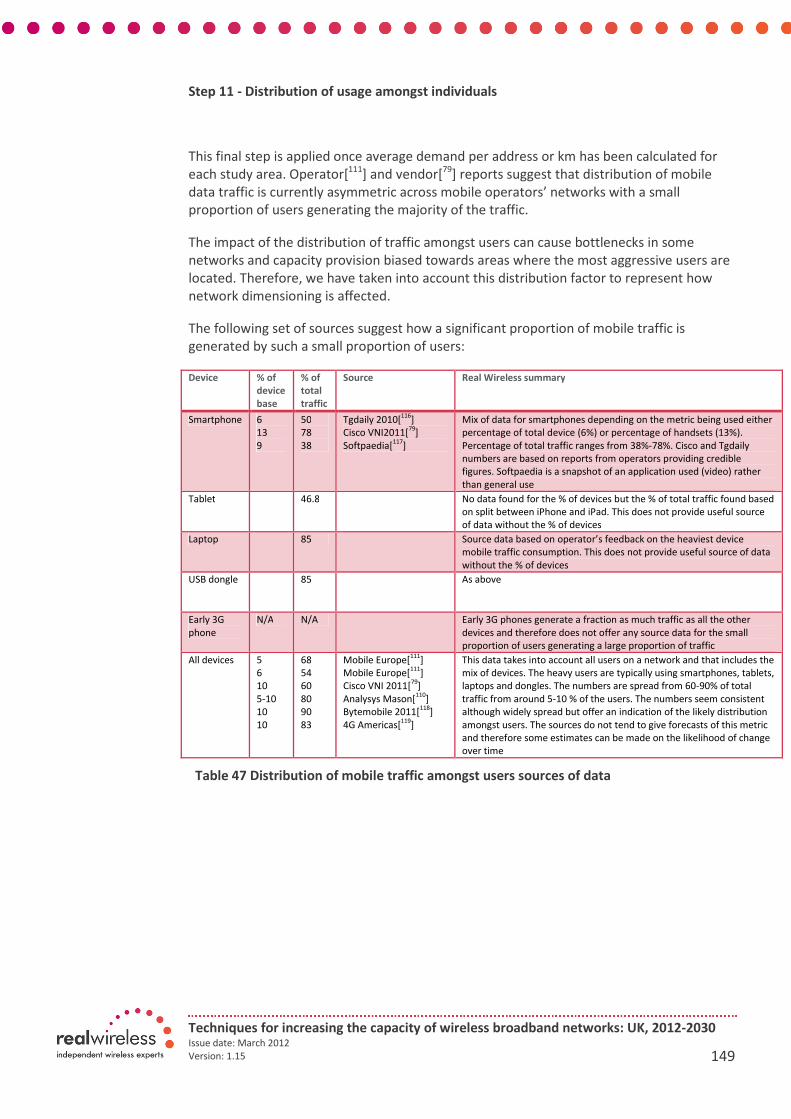
Techniques for increasing the capacity of wireless broadband networks: UK, 2012-2030 Issue date: March 2012
Version: 1.15 149
Step 11 - Distribution of usage amongst individuals
This final step is applied once average demand per address or km has been calculated for
each study area. Operator[111
] and vendor[79
] reports suggest that distribution of mobile
data traffic is currently asymmetric across mobile operators’ networks with a small
proportion of users generating the majority of the traffic.
The impact of the distribution of traffic amongst users can cause bottlenecks in some
networks and capacity provision biased towards areas where the most aggressive users are
located. Therefore, we have taken into account this distribution factor to represent how
network dimensioning is affected.
The following set of sources suggest how a significant proportion of mobile traffic is
generated by such a small proportion of users:
Device % of
device
base
% of
total
traffic
Source Real Wireless summary
Smartphone 6
13
9
50
78
38
Tgdaily 2010[116
]
Cisco VNI2011[79
]
Softpaedia[117
]
Mix of data for smartphones depending on the metric being used either
percentage of total device (6%) or percentage of handsets (13%).
Percentage of total traffic ranges from 38%-78%. Cisco and Tgdaily
numbers are based on reports from operators providing credible
figures. Softpaedia is a snapshot of an application used (video) rather
than general use
Tablet 46.8 No data found for the % of devices but the % of total traffic found based
on split between iPhone and iPad. This does not provide useful source
of data without the % of devices
Laptop 85 Source data based on operator’s feedback on the heaviest device
mobile traffic consumption. This does not provide useful source of data
without the % of devices
USB dongle 85 As above
Early 3G
phone
N/A N/A Early 3G phones generate a fraction as much traffic as all the other
devices and therefore does not offer any source data for the small
proportion of users generating a large proportion of traffic
All devices 5
6
10
5-10
10
10
68
54
60
80
90
83
Mobile Europe[111
]
Mobile Europe[111
]
Cisco VNI 2011[79
]
Analysys Mason[110
]
Bytemobile 2011[118
]
4G Americas[119
]
This data takes into account all users on a network and that includes the
mix of devices. The heavy users are typically using smartphones, tablets,
laptops and dongles. The numbers are spread from 60-90% of total
traffic from around 5-10 % of the users. The numbers seem consistent
although widely spread but offer an indication of the likely distribution
amongst users. The sources do not tend to give forecasts of this metric
and therefore some estimates can be made on the likelihood of change
over time
Table 47 Distribution of mobile traffic amongst users sources of data

Techniques for increasing the capacity of wireless broadband networks: UK, 2012-2030 Issue date: March 2012
Version: 1.15 150
Table 47 shows the data of distribution of traffic amongst users from the various sources
which include a mix of independent analysts, industry web sites and equipment vendors.
There was little specific data across the different devices, apart from smartphones where
three particular sources provided an inconsistent mix of data. The data that was most
consistent in terms of similar distribution values was that for all mobile traffic irrespective
of device. Therefore, it was this data that was used to determine the distribution of mobile
traffic amongst users.
• Starting point in 2012 is 10% of users consume 80% of the traffic
• In terms of variation of this metric over time Cisco VNI 2011[79
] found that
distribution of traffic amongst users is becoming more uniform over time. The
table extracted below shows the top 1% of users generating 29% of traffic in
month 1 and declining over time to 22% of traffic by month 9.
Therefore, we propose to base our variation over time assumptions on a similar decline in
non-uniform distribution of mobile traffic amongst users. We expect the rate of change to
start at similar rate to that of the Cisco numbers for the first five years and then to slow
down to a constant rate from 2017 to 2030 as traffic becomes more uniform.
Device % of
user
base
(2012)
% of total traffic
(2012)
Growth assumptions
Across
all
devices
10 80 10% of users use 80 traffic in 2012
• This is based on sources shown in Table 47
10% of users use 45% traffic by 2017
• This is based on growth rate similar to that of the Cisco VNI findings for
increased uniformity of traffic
10% of users use 38% traffic by 2020
• This is based on a slight slow down in growing uniformity as a wider
proportion of users are already generating a higher proportion of
the traffic
10% of device base 28% traffic by 2030
• The trend from 2020 to 2030 slows pace as traffic saturates in some
hot spot areas
Table 48 Real Wireless proposal for growth of distribution of traffic amongst individuals

Techniques for increasing the capacity of wireless broadband networks: UK, 2012-2030 Issue date: March 2012
Version: 1.15 151
Figure 5-35 Evolution of distribution of traffic amongst individuals over time
0%
10%
20%
30%
40%
50%
60%
70%
80%
90%
100%
0% 10% 20% 30% 40% 50% 60% 70% 80% 90% 100%
% traffic (cumulative)
% Users
% traffic (published) 4GAmericas
rW equation against published 2012
rW equation against Cisco
Cisco month 1
Cisco Month 9
rW equation 2017
rW equation 2020
rW equation 2030
Techniques for increasing the capacity of wireless broadband networks: UK, 2012-2030 Issue date: March 2012
Version: 1.15 152
A6. Technical model description
6.1 Introduction
This section describes the modelling framework that was set up in order to estimate the
cost of upgrading a mobile network in the period of interest 2020 to 2030. The inputs to
this model are listed and explained. Several algorithms are discussed and the form of
output is presented. The model combines together several pieces of previous modelling
work by Real Wireless into a comprehensive overall framework for network capacity
evolution, sensitive to both technical characteristics and financial metrics of benefit.
6.2 Brief description
The model accepts several inputs, such as the spectrum scenarios or the expected spectral
efficiency, performs a series of decisions to upgrade the 2012’s network to 2030 based on
cost effectiveness, and outputs the cost of performing these decisions. Three study areas
were identified to run the model, each with distinct propagation characteristics.
6.2.1 Prior to first modelled year
In each run, the model reads the following inputs which are varied across scenario runs
• Spectral efficiency
• Available spectrum quantities from all modelled bands (17 bands in total)
• Average demand (Mbps/demand point) in three hours of a busy day
• Offloaded demand
The model begins by plotting a map of the study area and populating this map with demand
points, which are locations where traffic demand is requested. A buffer area is added
externally around the study are to mitigate edge effects. Results are reported for the study
area.
The demand locations are real geographical locations of postcodes and locations along real
roads and railways that run through the study area. Each demand point corresponds to a
number of domestic and business delivery addresses, if the demand point is a postcode, or
to a transport type, see Table 49. Although the demand points do not have clutter
information assigned to them, a clutter database is used to determine the geotype where
the demand point lies on. Three geotypes are considered in this model, namely urban,
suburban and rural.
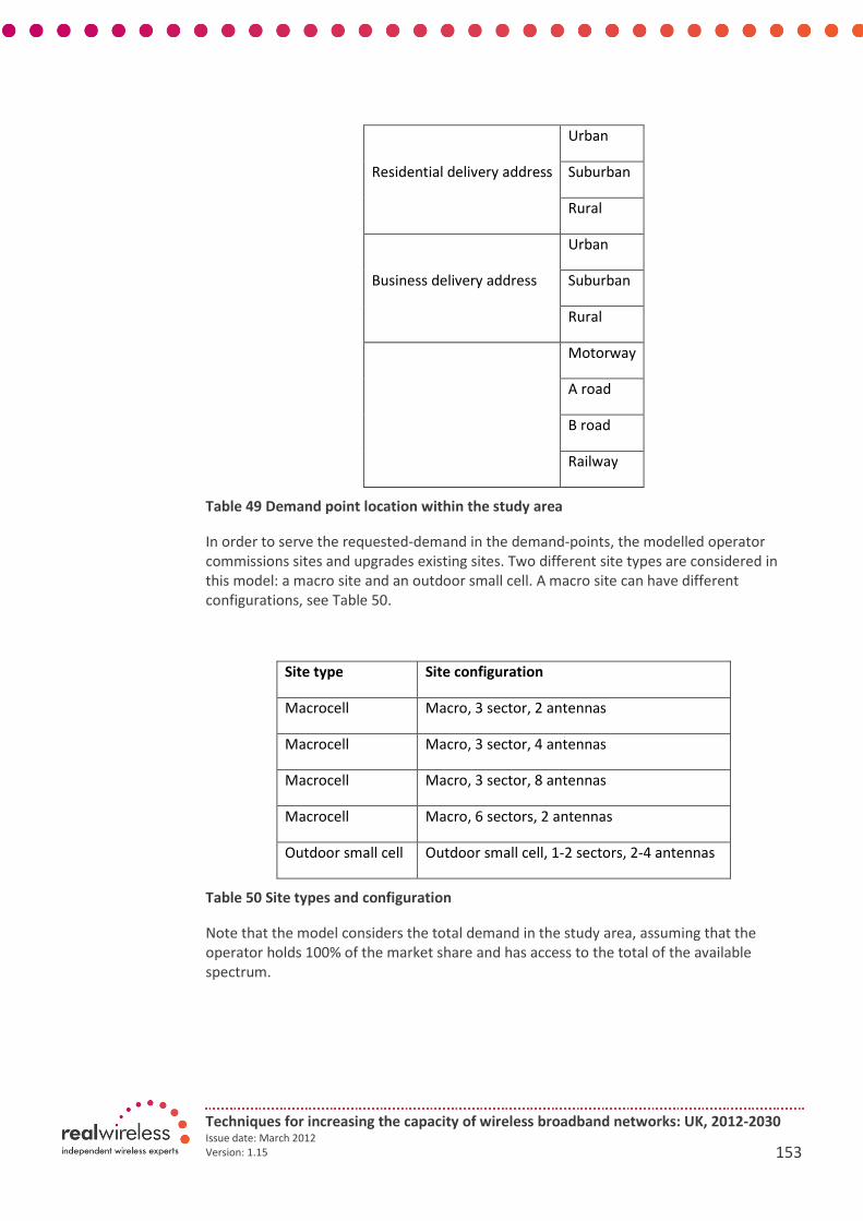
Techniques for increasing the capacity of wireless broadband networks: UK, 2012-2030 Issue date: March 2012
Version: 1.15 153
Residential delivery address
Urban
Suburban
Rural
Business delivery address
Urban
Suburban
Rural
Motorway
A road
B road
Railway
Table 49 Demand point location within the study area
In order to serve the requested-demand in the demand-points, the modelled operator
commissions sites and upgrades existing sites. Two different site types are considered in
this model: a macro site and an outdoor small cell. A macro site can have different
configurations, see Table 50.
Site type Site configuration
Macrocell Macro, 3 sector, 2 antennas
Macrocell Macro, 3 sector, 4 antennas
Macrocell Macro, 3 sector, 8 antennas
Macrocell Macro, 6 sectors, 2 antennas
Outdoor small cell Outdoor small cell, 1-2 sectors, 2-4 antennas
Table 50 Site types and configuration
Note that the model considers the total demand in the study area, assuming that the
operator holds 100% of the market share and has access to the total of the available
spectrum.
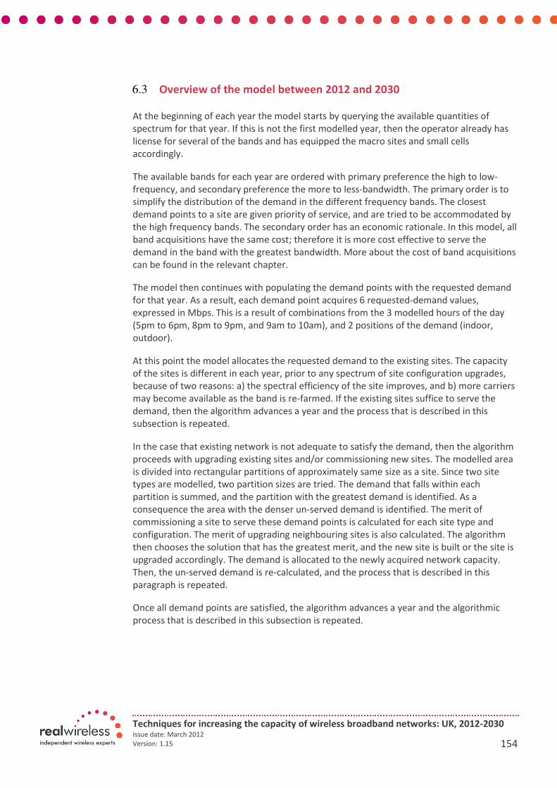
Techniques for increasing the capacity of wireless broadband networks: UK, 2012-2030 Issue date: March 2012
Version: 1.15 154
6.3 Overview of the model between 2012 and 2030
At the beginning of each year the model starts by querying the available quantities of
spectrum for that year. If this is not the first modelled year, then the operator already has
license for several of the bands and has equipped the macro sites and small cells
accordingly.
The available bands for each year are ordered with primary preference the high to low-
frequency, and secondary preference the more to less-bandwidth. The primary order is to
simplify the distribution of the demand in the different frequency bands. The closest
demand points to a site are given priority of service, and are tried to be accommodated by
the high frequency bands. The secondary order has an economic rationale. In this model, all
band acquisitions have the same cost; therefore it is more cost effective to serve the
demand in the band with the greatest bandwidth. More about the cost of band acquisitions
can be found in the relevant chapter.
The model then continues with populating the demand points with the requested demand
for that year. As a result, each demand point acquires 6 requested-demand values,
expressed in Mbps. This is a result of combinations from the 3 modelled hours of the day
(5pm to 6pm, 8pm to 9pm, and 9am to 10am), and 2 positions of the demand (indoor,
outdoor).
At this point the model allocates the requested demand to the existing sites. The capacity
of the sites is different in each year, prior to any spectrum of site configuration upgrades,
because of two reasons: a) the spectral efficiency of the site improves, and b) more carriers
may become available as the band is re-farmed. If the existing sites suffice to serve the
demand, then the algorithm advances a year and the process that is described in this
subsection is repeated.
In the case that existing network is not adequate to satisfy the demand, then the algorithm
proceeds with upgrading existing sites and/or commissioning new sites. The modelled area
is divided into rectangular partitions of approximately same size as a site. Since two site
types are modelled, two partition sizes are tried. The demand that falls within each
partition is summed, and the partition with the greatest demand is identified. As a
consequence the area with the denser un-served demand is identified. The merit of
commissioning a site to serve these demand points is calculated for each site type and
configuration. The merit of upgrading neighbouring sites is also calculated. The algorithm
then chooses the solution that has the greatest merit, and the new site is built or the site is
upgraded accordingly. The demand is allocated to the newly acquired network capacity.
Then, the un-served demand is re-calculated, and the process that is described in this
paragraph is repeated.
Once all demand points are satisfied, the algorithm advances a year and the algorithmic
process that is described in this subsection is repeated.
Techniques for increasing the capacity of wireless broadband networks: UK, 2012-2030 Issue date: March 2012
Version: 1.15 155
6.4 Flowchart
6.4.1 Flowchart overview
The model that calculates the cost of upgrading a mobile network in the period of interest
2020 to 2030 comprises of a sequence of algorithmic steps. These can be captured in a
flowchart. In this subsection a series of flowcharts is presented.
The model’s algorithm starts with the main flowchart of Figure 6-1. The model starts with a
pre-processing step. In this step the necessary variable are constructed so as to prepare the
inputs to the code. Then, these inputs are inserted in the next algorithmic block, where the
network is built from 0 macro and 0 small cells to several macros and small cells. The site
commissioning represents the mobile network in year 2012, which is the starting year in
this model.
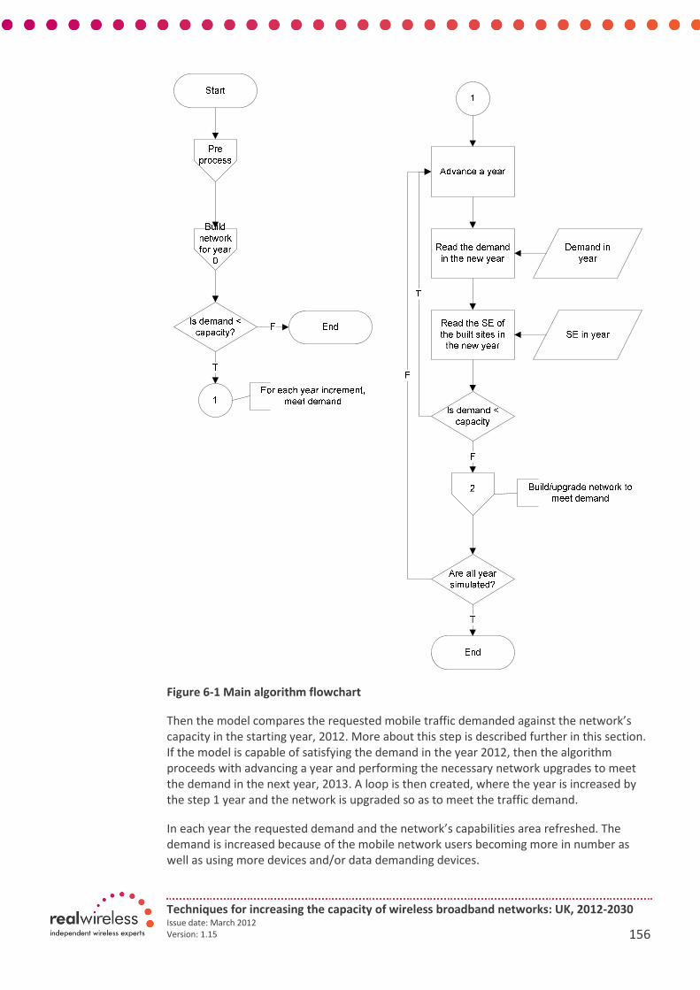
Techniques for increasing the capacity of wireless broadband networks: UK, 2012-2030 Issue date: March 2012
Version: 1.15 156
Figure 6-1 Main algorithm flowchart
Then the model compares the requested mobile traffic demanded against the network’s
capacity in the starting year, 2012. More about this step is described further in this section.
If the model is capable of satisfying the demand in the year 2012, then the algorithm
proceeds with advancing a year and performing the necessary network upgrades to meet
the demand in the next year, 2013. A loop is then created, where the year is increased by
the step 1 year and the network is upgraded so as to meet the traffic demand.
In each year the requested demand and the network’s capabilities area refreshed. The
demand is increased because of the mobile network users becoming more in number as
well as using more devices and/or data demanding devices.

Techniques for increasing the capacity of wireless broadband networks: UK, 2012-2030 Issue date: March 2012
Version: 1.15 157
The network’s capabilities also change each year. For example the user’s expectations
dictate the site ranges, so that the network’s coverage area shrinks. The spectral efficiency
increases as a result of improved network interfaces and hardware implementations. More
bandwidth also may become available in bands that the operator has already license for.
More information on the technical capabilities of the network and the increase of the
demand is provided in the chapter 3 of the main report.
6.5 Model calibration in year 2012
The requested demand is a model’s input. In the year 2012, we have a more informative
insight about the traffic demand and the network’s capabilities to serve it, compared to
future years. We know for example the number of 3G carriers that will be switched on in
several parts of the UK. Thus we are able to perform a model’s calibration with respect to
our expectations in 2012. The number of sites that are built by the model for the year 2012
was calibrated so that in the Central London study area it is roughly the same as existing
operator networks.
The model’s calibration was conducted against the Central London study area, and thus
other study areas’ network’s size is expected to deviate from real mobile network
deployments. Since modelling the coverage of notspots is not within the scopes of this
study, in all study areas we consider that coverage is provided in all demand locations,
regardless of today’s networks coverage maps. Therefore, after having calibrated the
network’s size, macros and outdoor small cells, in the Central London study area, the
network’s size in other study areas is expected to be higher than what the operators have
deployed. This is because we expect the operator’s coverage extent to be less than that of
the Central London study area.
6.6 Pre-processing of data
The model performs site building and upgrading based on the demand in the study area,
the network’s capabilities and the cost of new sites or site upgrades. In order to perform
the above actions, the model uses data from several files, e.g. demand, spectral efficiency,
offload, etc. The model also loads up several decision making constants that affect the
model’s performance. In this subsection the input files that are loaded for the model to
work are listed out and discussed.
In each run, the model reads the following inputs which are required for the scenario runs
• Grouping of the bands into three broad frequency categories (sub-1GHz, 1 to 2.1
GHz, and above-2.1 GHz)
• Spot frequency of each modelled band
• Distribution of the demand amongst stationary users (domestic and business)
• Split of the traffic between indoor and outdoor
• Cost of new sites (macro sites and outdoor small cells) and cost of upgrades of
macro sites. Outdoor small cells are assumed to be upgraded on their 5th
birthday, and this cost is included in their commissioning PV.
• Site ranges
• Capacity of offload devices, e.g. femtocells and Wi-Fi

Techniques for increasing the capacity of wireless broadband networks: UK, 2012-2030 Issue date: March 2012
Version: 1.15 158
Table 51 below provides a list of the model’s constants. Figure 6-2 shows a schematic of the
algorithmic steps in the pre-processing step of the model.
Name Description Value
Random seed A random seed is used for distributing the
demand amongst users, in domestic and
business addresses
Random seed for
the distribution
Buffer zone about
the focus area
A buffer zone is included in each study area
to build sites that could serve demand in the
focus area. Site in the focus area can also
serve demand in the buffer area. For time
saving purposes, we assumed that the
demand does not grow in the buffer zone as
time advances.
14km rural
2.5km suburban
1.5km urban
Minimum inter site
distance
A minimum separation distance between
macro sites, and a minimum distance
between small cells is applied to avoid the
algorithm placing sites too close together.
This is based on technical challenges of
increased interference when sites are
positioned very close.
340m macro,
corresponding to 10
sites/km2
18m outdoor small
cell, corresponding
to similar LOS
probability as 340m
for macros
Macro site
commissioning cost,
as a function of the
local average site
density
The commissioning of a new macro site is a
function of the local average macro site
density. For each new site, the neighbouring
macro sites are identified and the local site
density is calculated.
0sites/km2 for the
low cost site
10sites/km2 for the
high cost site
Weighting function
for the
determination of
the neighbouring
sites
0.2*σ leads to
approximately 8
neighbouring sites
Replacement cycle
of outdoor small
cells
Outdoor small cells area replaced on their 5th
birthday
5 years
Maximum number
of neighbours for
upgrade trial
Having identified the area where the demand
is not satisfied, the algorithm examines the
merit of upgrading a number of sites in the
area. The closest sites to the centroid of the
local under-served demand are listed. This
list is chopped at the 6 closest sites, however
it is provisioned that 1 macro is always
6 sites

Techniques for increasing the capacity of wireless broadband networks: UK, 2012-2030 Issue date: March 2012
Version: 1.15 159
existent in the list of potential site upgrades.
Demand peak to
mean ratio
The demand is calculated initially as an
average value in three modelled hours of a
busy day. In order to capture the effect of
the demand fluctuation within the busy hour,
the demand is multiplied with a peak to
mean ratio. This was selected 1:20, so that
the user expectation is 20 times larger than
the hourly average, e.g. a user is expected to
download a 6 MB email in 3 sec instead of 1
min, if the hourly speed is 0.8 Mbps and the
peak speed is 20 times the hourly speed. This
peak to mean ratio was calibrated in the
Central London study area so that the
requested demand populates the network
sites and carriers with roughly the same
network size as that expected by 2012
existing operators.
1:20
Road and rail
database
The Meridian 2 DXF data base is loaded. The
demand points in the model include locations
along the length of this database’s transport
lines. The transport lines were converted into
a matrix of equidistant demand locations,
with a different separation distance in each
study area, so that the resulting number of
demand points is manageable. As a result of
this conversion, the traffic junctions have a
higher demand than the length of the
transport lines. Several simplifications were
required in this conversion, so as to treat
transport lines that either run parallel to
boundary lines, penetrate transport lines
multiple times, or have a small length.
Motorway, A road, B
road, Railway
Focus area
boundary lines
database
The Ordnance Survey’s Boundary Line is
loaded
Addresses database The Geopoint database was loaded. The
demand points in the model include locations
of domestic and business addresses from this
database. PO boxes were not included in the
demand locations.
Clutter database The InfoTerra UK Sea data base is loaded.
This database determines 10 types in a
50x50m grid. For the purpose of this exercise
these types were reduced to 3 broader
clutter types, namely urban, suburban and

Techniques for increasing the capacity of wireless broadband networks: UK, 2012-2030 Issue date: March 2012
Version: 1.15 160
rural/open. These should not be confused
with the naming of the study areas. For
example the Rural Lincolnshire study area
includes urban, suburban and rural clutter
pixels.
Each demand point acquires the clutter type
of the 50x50m pixel where it lies. This affects
its ‘visibility’ by the network sites. For
example, an indoor urban address that is
1km from a site is not ‘visible’ from the site if
the urban site range < 1km, whereas an
indoor suburban address that is 1km from a
site is ‘visible’ if the suburban address > 1km.
Optimisation
reduction factor
The merit maximisation algorithm reduces
the size of the search area (i.e. the rectangle
with the greatest demand density) by this
factor, with the aim to find the most cost
effective site location.
Golden ratio
Table 51 Model constants list

Techniques for increasing the capacity of wireless broadband networks: UK, 2012-2030 Issue date: March 2012
Version: 1.15 161
Figure 6-2 Pre-process flowchart of algorithmic steps
Output
from
demand
model
Techniques for increasing the capacity of wireless broadband networks: UK, 2012-2030 Issue date: March 2012
Version: 1.15 162
6.7 New sites and site upgrades
This subsection provides information about the algorithmic processes that take place when
the model pursues to match the requested demand by building new sites or upgrading
existing sites. The algorithmic steps are similar, regardless of whether the network is built
for the first modelled year, 2012, or for future years. The exception is that in the starting
year, 2012, the network is built up from 0 macro sites and 0 small cells, towards satisfying
all the demand in the focus of the study area, without any upgrade options.
At the start of each modelled year the model updates the indices to the input entries. Table
52 summarises the input entries that are loaded from the input files.
Input Varies with
Cost of macro site commissioning (low
density)
Cost of macro site commissioning (high
density)
Range of macros and small cells Clutter type and frequency group
Spectral efficiency Frequency group
Spectrum quantity Spectrum band
Offload for stationary indoor demand
points
Clutter type and demand address type
(domestic/business)
Distribution of traffic amongst
stationary users
Offload device capacity
Table 52 Input entries for the model
After preparing the input data, the model sorts the available bands on the modelled year
with a preference order for serving the demand. The order is from high to low frequency-
group, and from high to low bandwidth. The model continues with creating a map of the
demand points in the modelled area, and calculating the rectangle dimensions where the
demand density is found. More details about these algorithmic processes are provided in
the previous section.

Techniques for increasing the capacity of wireless broadband networks: UK, 2012-2030 Issue date: March 2012
Version: 1.15 163
For each site configuration and site type, the site-location search algorithm identifies the
position of the site that leads to the greatest merit. During this part of the location search,
the merit is calculated using the maximum captured demand within the site’s range,
ignoring any capacity limitations. This is done because the operator would choose the best
locations for serving the demand, knowing in advance that several technical advances and
spectrum acquisitions will eventually increase the served demand that can be satisfied by a
capacity-constrained site. At the end of this algorithmic process, the site location and site
type & configuration that lead to the greatest merit have been calculated.
The algorithm then calculates the merit of upgrading sites. With respect to the identified
site location with the greatest merit, the model calculates the distance to all existing sites.
The merit of the site commissioning, for the identified location and site configuration, is
calculated, this time by taking into account the site’s capacity. For each of the closest
neighbours, the merit of an upgrade is also calculated. Outdoor small cells that have a life
duration of more than 5 years are replaced with new cells, without inducing a spectrum
upgrade cost, since the replacement cost has been included in the installation cost. If there
are no small cells within the neighbours, which can be upgraded for zero cost, spectrum
and configuration upgrade options are tried for macro sites within the neighbour list.
In all tried spectrum and configuration upgrade options, the merit is calculated for
comparison amongst the different options to provide coverage to the un-served demand.
The merit is defined as the amount of captured un-served demand, expressed in Mbps,
over the cost of the upgrade or commissioning.
The upgrade, or the commissioning, that has the greatest merit is identified and takes
place. The un-served demand is allocated to the newly acquired capacity, and the demand
map is refreshed to take into account the network upgrade.
The following flowchart presents the algorithmic steps for building the network for year
2012.

Techniques for increasing the capacity of wireless broadband networks: UK, 2012-2030 Issue date: March 2012
Version: 1.15 164
X
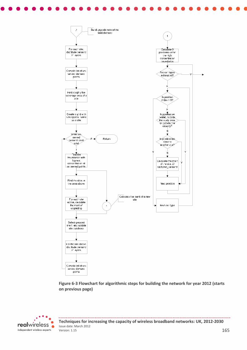
Techniques for increasing the capacity of wireless broadband networks: UK, 2012-2030 Issue date: March 2012
Version: 1.15 165
Figure 6-3 Flowchart for algorithmic steps for building the network for year 2012 (starts
on previous page)

Techniques for increasing the capacity of wireless broadband networks: UK, 2012-2030 Issue date: March 2012
Version: 1.15 166
6.8 Modelling of spectrum
The available quantity of spectrum in each year is an input to the model. The model reads
the available spectrum quantities and converts it to network capacity. This section
discusses how the spectrum is used by the model in order to satisfy the requested demand
in each year.
The spectrum input consists of a table of values, one row for each modelled band and one
column for each modelled year. See Table 53. The values of this table are expressed in MHz.
In each year the model reads the available bandwidth for each band. If the bandwidth is 0,
then the band is assumed not be available. For example, there is 0MHz in 900MHz in 2012
in the rural Lincolnshire study area, whereas there is 5MHz in the same band and year in
the Central London study area
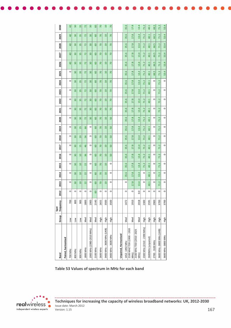
Techniques for increasing the capacity of wireless broadband networks: UK, 2012-2030 Issue date: March 2012
Version: 1.15 167
Table 53 Values of spectrum in MHz for each band
Ba
nd
G
rou
p
Sp
ot
fre
qu
en
cy
20
12
2
01
3
20
14
2
01
5
20
16
2
01
7
20
18
2
01
9
20
20
2
02
1
20
22
2
02
3
20
24
2
02
5
20
26
2
02
7
20
28
2
02
9
20
30
Pa
ire
d,
ha
rmo
nis
ed
70
0 M
Hz
Low
7
00
0
0
0
0
0
0
0
0
0
0
0
0
0
0
4
0
40
4
0
40
4
0
80
0 M
Hz
Low
8
00
0
3
0
30
3
0
30
3
0
30
3
0
30
3
0
30
3
0
30
3
0
30
3
0
30
3
0
30
90
0 M
Hz
Low
9
00
0
1
0
10
1
0
10
1
5
20
2
5
30
3
5
35
3
5
35
3
5
35
3
5
35
3
5
35
18
00
MH
z M
ed
1
80
0
0
22
2
2
22
3
6
46
5
6
66
7
2
72
7
2
72
7
2
72
7
2
72
7
2
72
7
2
19
00
MH
z (1
98
0-2
01
0 M
Hz)
M
ed
1
90
0
0
0
0
0
0
0
0
0
30
3
0
30
3
0
30
3
0
30
3
0
30
3
0
30
21
00
MH
z M
ed
2
14
0
60
6
0
60
6
0
60
6
0
60
6
0
60
6
0
60
6
0
60
6
0
60
6
0
60
6
0
60
26
00
MH
z H
igh
2
65
5
0
70
7
0
70
7
0
70
7
0
70
7
0
70
7
0
70
7
0
70
7
0
70
7
0
70
7
0
34
00
MH
z -
36
00
MH
z (U
KB
) H
igh
3
50
0
0
10
1
0
10
1
0
10
1
0
10
1
0
10
1
0
10
1
0
10
1
0
10
1
0
10
1
0
34
00
MH
z -
36
00
MH
z H
igh
3
50
0
0
0
0
0
50
5
0
50
5
0
50
7
0
70
7
0
70
7
0
70
7
0
70
7
0
70
Un
pa
ire
d,
Ha
rmo
nis
ed
14
52
-1
49
2 M
Hz
Me
d
14
72
0
0
3
5.6
3
5.6
3
5.6
3
5.6
3
5.6
3
5.6
3
5.6
3
5.6
3
5.6
3
5.6
3
5.6
3
5.6
3
5.6
3
5.6
3
5.6
3
5.6
3
5.6
21
00
MH
Z T
DD
(1
90
0 -
19
20
MH
z)
Me
d
19
10
0
1
7.8
1
7.8
1
7.8
1
7.8
1
7.8
1
7.8
1
7.8
1
7.8
1
7.8
1
7.8
1
7.8
1
7.8
1
7.8
1
7.8
1
7.8
1
7.8
1
7.8
1
7.8
21
00
MH
z T
DD
(2
01
0 -
20
25
MH
z)
Me
d
20
18
0
.0
13
.4
13
.4
13
.4
13
.4
13
.4
13
.4
13
.4
13
.4
13
.4
13
.4
13
.4
13
.4
13
.4
13
.4
13
.4
13
.4
13
.4
13
.4
23
00
MH
z (2
31
0 -
23
90
MH
z)
Hig
h
23
00
0
0
0
7
1.2
7
1.2
7
1.2
7
1.2
7
1.2
7
1.2
7
1.2
7
1.2
7
1.2
7
1.2
7
1.2
7
1.2
7
1.2
7
1.2
7
1.2
7
1.2
26
00
MH
z (u
np
air
ed
) H
igh
2
59
5
0
40
.1
40
.1
40
.1
40
.1
40
.1
40
.1
40
.1
40
.1
40
.1
40
.1
40
.1
40
.1
40
.1
40
.1
40
.1
40
.1
40
.1
40
.1
27
00
- 3
10
0 M
Hz
Hig
h
29
00
0
0
0
0
0
0
0
0
0
0
0
0
0
4
4.5
4
4.5
4
4.5
4
4.5
4
4.5
4
4.5
36
00
MH
z -3
80
0 M
Hz
(UK
B)
Hig
h
37
00
0
7
1.2
7
1.2
7
1.2
7
1.2
7
1.2
7
1.2
7
1.2
7
1.2
7
1.2
7
1.2
7
1.2
7
1.2
7
1.2
7
1.2
7
1.2
7
1.2
7
1.2
7
1.2
36
00
MH
z -3
80
0 M
Hz
Hig
h
37
00
0
0
0
0
0
0
0
0
0
0
0
0
0
5
3.4
5
3.4
5
3.4
5
3.4
5
3.4
5
3.4
Techniques for increasing the capacity of wireless broadband networks: UK, 2012-2030 Issue date: March 2012
Version: 1.15 168
It is noted that, the band availability in a year does not force the operator to use the
available band, i.e. the modelled operator can choose from the available bands. If the
model finds that is cost effective for the operator to upgrade the technology of a macro site
to support a band that the macro did not previously support, then this incurs a spectrum
upgrade cost. All new commissioning of macro sites are assumed to support all bands that
the operator has licence for, i.e. the union of supported bands across all macro sites in the
commissioning year.
It is assumed in this model that all macro spectrum upgrades have the same cost. This is
because the cost is closer related to the upgrade requirement, rather than the amount of
additional bands that need to be supported. It is assumed that it is more cost effective for
the modelled operator to acquire the band with the largest bandwidth first, so as to
maximise the increase of the site’s capacity. In order to refrain the operator from upgrading
to support all the available bands at once, the model assumes that the modelled operator
will upgrade to that many additional bands so that the demand is satisfied. This means that
the operator can upgrade a macro site to support e.g. 9 additional bands, see Table 53, if
the demand is large enough, however it will upgrade to support a smaller number of bands,
if the demand is lower.
Small cells can only be upgraded on their fifth birthday, or later. Depending on the year a
different number of bands is supported.
Based on the above, the order of preference in filling-in the bands with demand is from
bands of larger- to smaller-bandwidth. This is the secondary order of preference, whereas
the primary order is from bands with a higher- to lower-frequency. For the primary order of
preference the frequency group is used, rather than the spot frequency, see Table 53. The
primary order is required because the demand points are accommodated in the bands
starting from the closest- to the furthest-point. Thus the closest points will be sought to be
accommodated by the high frequency bands, whereas further points by the low frequency.
The primary and secondary order of preference are also discussed below in an example.
Figure 6-4plot the band utilisation output from Scenario 18, Rural Lincolnshire, introduction
of the 700MHz band in 2026, low demand, high offload of demand, high spectrum
availability. This scenario corresponds to the spectrum input of Table 53. The utilisation of
each band is plotted for each year and band. The utilisation is defined as the ratio of the
demand that is accommodated in a band over the total demand (capacity) that the band
can accommodate. Each site has a different utilisation of its spectrum resources. The
plotted curves correspond to the average across all macro sites.

Techniques for increasing the capacity of wireless broadband networks: UK, 2012-2030 Issue date: March 2012
Version: 1.15 169
Figure 6-4 Frequency band utilisation output from scenario 18 rural Lincolnshire low
demand/high capacity 2026
In 2012, only the 2100MHz is available, and this band about 50% utilised. This means that
there are several sites that are fully utilising this band; however there are a large number of
sites that provide coverage. The reader is advised to compare this figure against a similar
one for the Central London study area, where the band utilisation is close to 100%. In 2013,
a large number of bands become available to the modelled operator. Out of the 9 new
bands, the operator chooses the low frequency band that offers the greatest capacity, i.e.
the 800MHz band. This is because the un-served demand-points in 2013 are at the outskirts
of several sites, and a low frequency band is able to reach and serve them. The demand
also increases closer to the sites, thus the 2100 MHz band utilisation increases.
In 2014, one or more macro sites run out of capacity, and they are upgraded to support two
new bands, namely the TDD 1452 -1492 MHz and the TDD 3600 MHz -3800 MHz. The
former band is used as an alternative to the fully utilised – in that site –2100 MHz, since it
boasts the greatest bandwidth amongst the medium frequency bands. The latter band is
used for even more capacity close to the site, since it boasts the greatest bandwidth
amongst the high frequency bands. However, since most sites have not run out of capacity
and therefore have not been upgraded to support these two bands, the band utilisation of
these bands is quite low. In the same year, several sites are upgraded to support the
800MHz band to provide coverage to demand-points that were left outside the shrinking
site ranges. Further, the 2100 MHz band utilisation continues to rise, because of the
increasing demand in all sites.
In 2015, more sites require spectrum upgrade as a consequence of the increased demand
filling-up their capacity. The bands that are best candidates to accommodate the demand
are: the 800MHz for far points, the TDD 1452 -1492 MHz for medium distance points, and
700 MHz
800 MHz1800 MHz
2100 MHz
0%
10%
20%
30%
40%
50%
60%
70%
80%
90%
100%
20
12
20
13
20
14
20
15
20
16
20
17
20
18
20
19
20
20
20
21
20
22
20
23
20
24
20
25
20
26
20
27
20
28
20
29
20
30
Ba
nd
uti
lisa
tio
n
700 MHz
800 MHz
900 MHz
1800 MHz
1900 MHz (1980-2010 MHz)
2100 MHz
2600 MHz
3400 MHz - 3600 MHz (UKB)
3400 MHz - 3600 MHz
1452 -1492 MHz
2100 MHZ TDD (1900 - 1920 MHz)
2100 MHz TDD (2010 -2025 MHz)
2300 MHz (2310 - 2390 MHz)
2600MHz
2700 - 3100 MHz
3600 MHz -3800 MHz (UKB)
3600 MHz -3800 MHz

Techniques for increasing the capacity of wireless broadband networks: UK, 2012-2030 Issue date: March 2012
Version: 1.15 170
the TDD 2300 MHz (2310 - 2390 MHz) for close points. The latter offers the same capacity
as the favourite high-frequency band of the previous year, TDD 3600 MHz -3800 MHz, but is
further up in the rows of the spectrum table.
The demand continues to be accommodated in each band, in each site independently,
according to the needs for each site and the available spectrum in each year. There is an
interesting shift in the order of preference between years 2018 and 2019 in the medium-
frequency bands. In 2019, the 1800MHz band becomes more attractive than the 2100MHz.
This is reflected by the decline of the 2100 MHz band utilisation, and the sharp rise of the
1800 MHz band. Note that although the 2100 MHz utilisation declining trend is continuing
in the next years, the 1800 MHz band utilisation-curve does not rise as fast. This is because
the 1800 MHz bandwidth continues to increase in 2020. A similar shift in preference is
noticeable between the low frequency curves of 700 and 800 MHz.
As the total available bandwidth across all bands increases, through re-farming, without
need of further spectrum upgrades, the bandwidth utilisation curves are dragged
downwards, i.e. the bands are less utilised because of the total increase in spectrum.

Techniques for increasing the capacity of wireless broadband networks: UK, 2012-2030 Issue date: March 2012
Version: 1.15 171
References
1 Ofcom, “Application of spectrum liberalisation and trading to the mobile sector”
http://stakeholders.ofcom.org.uk/consultations/spectrumlib/, February 2009
2 ABI Research, “Multistandard base stations to reach 93% of total shipments by 2015”,
http://www.totaltele.com/view.aspx?ID=457030, July, 2010.
3 Ofcom, “Assessment of future mobile competition and proposals for the award of 800
MHz and 2.6 GHz spectrum and related issues”
http://stakeholders.ofcom.org.uk/consultations/combined-award/, March 2011.
4 Signals Research Group, “The Business Case for Femtocells in the Mobile Broadband Era”,
http://www.femtoforum.org/femto/pdfs01.php, March 2010
5 Ofcom, “The Communications Market, 2011”
http://stakeholders.ofcom.org.uk/binaries/research/cmr/cmr11/UK_Doc_Section_5.pdf
6 HMT, Supplementary Guidance on The Green Book – Appraisal and Evaluation in Central
Government, 2011, http://www.hm-treasury.gov.uk/data_greenbook_supguidance.htm
7 Europe Economics ”Economic impact of the use of radio spectrum in the UK”,
http://stakeholders.ofcom.org.uk/market-data-research/spectrum-
research/economic_spectrum_use/, 2006.
8 “Transition to 4G, 3GPP Broadband Evolution to IMT-Advanced (4G)”, Rysavvy Research &
3G Americas, September 2010
9 “MIMO Performance and Condition Number in LTE Test”, Agilent Application Note,
October 2009, http://cp.literature.agilent.com/litweb/pdf/5990-4759EN.pdf
10 “Field Trials of LTE with 4x4 MIMO”, Ericsson review, no. 1 2010,
http://www.ericsson.com/res/thecompany/docs/publications/ericsson_review/2010/ericss
onreview_issue1_2010.pdf
11 “Field Trials of LTE with 4x4 MIMO”, Ericsson review, no. 1 2010,
http://www.ericsson.com/res/thecompany/docs/publications/ericsson_review/2010/ericss
onreview_issue1_2010.pdf
12 “Further advancements for E-UTRA physical layer”, 3GPP TR 36.814, March 2010,
http://ftp.3gpp.org/specs/html-info/36814.htm
13 “Further advancements for E-UTRA physical layer”, 3GPP TR 36.814, March 2010,
http://ftp.3gpp.org/specs/html-info/36814.htm
14 “LTE User Equipment, network efficiency and value Mobile broadband radio access
economics - pre requisites for profitability”, G.Varrall, 2/9/2010
15 “Binary Power Control for Sum Rate Maximisation over Multiple Interfering Links”, A.
Gjendemsjoe et al, IEEE Trans. Wireless Communications, August 2008
16 “LTE The UMTS Long Term Evolution” S.Sesia et al, [Publisher and date to be inserted in
final report]
17 “Further advancements for E-UTRA physical layer aspects”, 3GPP TR 36.814
http://ftp.3gpp.org/specs/html-info/36814.htm
18 3GPP TR 36.912 v9.0.0, 3rd Generation Partnership Project; Technical Specification
Group Radio Access Network; Feasibility study for Further Advancements for EUTRA(LTE-
Advanced) (Release 9)
Techniques for increasing the capacity of wireless broadband networks: UK, 2012-2030 Issue date: March 2012
Version: 1.15 172
19 “3GPP Mobile Broadband Innovation Path to 4G: Release 9, Release 10 and Beyond:
HSPA+, SAE/LTE and LTE-Advanced”, 3G Americas. Feb 2010
http://www.3gamericas.org/index.cfm?fuseaction=register&goto=http://www.3gamer
icas.org/documents/3GPP_Rel-9_Beyond%20Feb%202010.pdf
20 “Centralized Scheduling for Joint Transmission Coordinated Multipoint in LTE-
Advanced”, St. Brueck, L. Zhao, J. Giese, and M. Awais Amin. International ITG/IEE
Workshop on Smart Antennas (WSA'10), Bremen, Germany, 23. - 24. February 2010.
21 “Downlink Coordinated Scheduling Simulation Results”, Ralph Ballentin, Mark Doll, VDE
ITG 5.2.4 Workshop Heidelberg 8. July 2010
22 “Femtocells – natural solution for offload”, Small Cell Forum white paper 016, June
2010, from http://www.smallcellforum.org/resources-white-papers
23 www.smallcellforum.org
24 “Interference management in UMTS femtocells”, Small Cell Forum white paper 009,
February 2010, http://www.smallcellforum.org/resources-white-papers
25 “Femto plugfest”, Light Reading, March 2010,
http://www.lightreading.com/blog.asp?blog_sectionid=414&doc_id=189942
26 “3GPP Mobile Broadband Innovation Path to 4G: Release 9, Release 10 and Beyond:
HSPA+, SAE/LTE and LTE-Advanced”, 3G Americas. Feb 2010
27 3GPP Release dates: http://www.3gpp.org/releases
28 3GPP Work plan (incl rel 12)
http://www.3gpp.org/ftp/Information/WORK_PLAN/Description_Releases/
29 “Future of Mobile Networks Report”, Informa, Media and Telecoms, 2010
30 "4G Capacity Gains", Real Wireless, January 2011,
http://stakeholders.ofcom.org.uk/market-data-research/technology-research/2011/4G-
Capacity-Gains/
31 PA Consulting Group, “Predicting Areas of Spectrum Shortages”, 7th April 2009,
http://stakeholders.ofcom.org.uk/binaries/research/technology-research/shortage.pdf
32 "Feasibility study for Further Advancements for E-UTRA (LTE-Advanced)" 3GPP TR
36.912 V9.3.0 (2010-06)
33 Further advancements for E-UTRA physical layer aspects, 3GPP TR 36.814 V9.0.0 (2010-
03)
34 “System Performance Challenges of IMT-Advanced Test Environments”, Per Burström et
al, Ericsson, PIMRC 2009, http://goo.gl/ObAqd
35 C. E. Shannon. The Mathematical Theory of Communication. Urbana, IL:University of
Illinois Press, (1949)
36 “Radio network planning and optimisation for UMTS”, Jaana Laiho et al, 2nd ed, Wiley
2006
37 “Small cell deployment strategy and challenges”, 8th Annual Base Station Conference,
27-29 September 2011
Peter Stevens / Zhongrong Liu, Deutsche Telekom, http://db.tt/E4bfYaPL
38 “Guidelines for evaluation of radio interface technologies for IMT-Advanced”, REPORT
ITU-R M.2135, 2008
39 “ESTIMATION OF THE POTENTIAL DEPLOYMENT OF SMALL CELL BASESTATIONS IN 2015”,
Picochip, 8th Annual Base Station Conference, 27 September 2011
40 Huawei HetNet Overview, Dr. Peter (Yuefeng) Zhou, Avren Base Station Conference,
Sept 2011, http://db.tt/WOZqtwZn
41 “Huawei Small Cell” , Michael Lemke, Informa Small Cell Forum, Berlin, Oct 11th 2011,
http://db.tt/9VfluWqB

Techniques for increasing the capacity of wireless broadband networks: UK, 2012-2030 Issue date: March 2012
Version: 1.15 173
42 Further consultation on the 800 MHz and 2.6 GHz competition assessment and award
proposals, to be published end of December 2011
43 “Transition to 4G, 3GPP Broadband Evolution to IMT-Advanced (4G)”, Rysavvy Research
& 3G Americas, September 2010
44 United Kingdom Frequency Allocation Table, UKSSC, 2010,
http://stakeholders.ofcom.org.uk/binaries/spectrum/spectrum-policy-area/spectrum-
management/ukfat2010.pdf
45 “Enabling UK growth – Releasing public spectrum Making 500 MHz of spectrum available
by 2020”, Department for Culture Media, March 2011,
http://www.culture.gov.uk/publications/7994.aspx
46 “Revised 700 MHz Band Plan for Commercial Services”, FCC, 2007
http://wireless.fcc.gov/auctions/data/bandplans/700MHzBandPlan.pdf
47 “Commission Decision 2010/267/EU” European Commission, 2010
http://www.erodocdb.dk/docs/doc98/official/pdf/2010267EU.pdf
48 “Update on plans for award of 800MHz and 2.6GHz spectrum”, Ofcom, October 2011,
http://stakeholders.ofcom.org.uk/consultations/combined-
award/update?utm_source=updates&utm_medium=email&utm_campaign=combined-
award-update
49 “UK Interface Requirement 2014 Public Wireless Networks”, Ofcom, Aug 2005,
http://stakeholders.ofcom.org.uk/binaries/spectrum/spectrum-policy-area/spectrum-
management/research-guidelines-tech-info/interface-requirements/ir2014.pdf
50 “Mobile Broadband Global Update and evolution”, GSA, June 2011
http://www.gsacom.com/downloads/pdf/GSA_MBB_Global_Update_June_2011.php4
51 “GSA Report status of the LTE ecosystem”, GSA, June 2011,
http://www.gsacom.com/downloads/pdf/GSA_LTE_ecosystem_report_June_2011_130611.
php4
52 “UK Interface Requirement 2019 Third Generation Mobile”, Ofcom, Aug 2005,
http://stakeholders.ofcom.org.uk/binaries/spectrum/spectrum-policy-area/spectrum-
management/research-guidelines-tech-info/interface-requirements/3gm.pdf
53 “ECC Decision of 18 March 2005 on harmonised utilisation of spectrum for IMT-
2000/UMTS systems operating within the band 2500 – 2690 MHz”, ECC Decision (05)05,
March 2005, http://www.erodocdb.dk/docs/doc98/official/pdf/ECCDec0505.pdf
54 54 “UK Interface Requirements 2015.1 to IR 2015.3 Spectrum Access in the 3400 to 4009
MHz band”, Ofcom, 2011, http://stakeholders.ofcom.org.uk/binaries/spectrum/spectrum-
policy-area/spectrum-management/research-guidelines-tech-info/interface-
requirements/Draft_IR_2015.pdf
55 3rd Generation Partnership Project; Technical Specification Group Radio Access
Network;
Evolved Universal Terrestrial Radio Access (E-UTRA); User Equipment (UE) radio
transmission and reception
(Release 9), 3GPP TS 36.101 v10.1.0, September 2011, http://www.3gpp.org/specifications
56 Benny Har-Even, “PCCW looking to build UK’s first LTE network”,
http://www.telecoms.com/29272/pccw-looking-to-build-uks-first-lte-network/, 16 June
2011
57 “E-UTRA Physical Channels and Modulation”, 3GPP TS 26.211 V10.3.0 (2011-09),
http://www.3gpp.org/ftp/Specs/html-info/36211.htm
58 ECC DEC 03(02) ECC Decision of 17 October 2003 on the designation of the frequency
band 1479.5 – 1492 MHz
Techniques for increasing the capacity of wireless broadband networks: UK, 2012-2030 Issue date: March 2012
Version: 1.15 174
for use by Satellite Digital Audio Broadcasting systems, European Commission, 2003,
http://www.erodocdb.dk/docs/doc98/official/pdf/ECCDec0302.pdf
59 “Economic study of the benefits from use of 1452-1492 MHz for a supplemental mobile
downlink for enhanced multimedia and broadband services “, Plum consulting, June 2011,
http://www.plumconsulting.co.uk/pdfs/Plum_June2011_Benefits_of_1.4GHz_spectrum_fo
r_multimedia_services.pdf
60 “Consultation on assessment of future mobile competition and proposals for the award
of 800 MHz and 2.6 GHz spectrum and related issues”, Ofcom, March 2011,
http://stakeholders.ofcom.org.uk/binaries/consultations/combined-
award/summary/combined-award.pdf
61 “White Paper LTE TDD Operator Business Case and Adoption Forecast”, Berge Ayvazian,
Heavy Reading, March 2011,
62 “O2 first to switch on new superfast 3G 900 MHz network”,
http://mediacentre.o2.co.uk/Press-Releases/O2-first-to-switch-on-new-superfast-3G-
900MHz-network-2f8.aspx
63 “Consultation and information on technical licence conditions for 800 MHz and 2.6 GHz
spectrum and related matters”, Ofcom, June 2011
64 “Low Power Shared Access to Mobile Broadband Spectrum”, Final Report to Ofcom by
Real Wireless, March 2011
65 Kathrein 742 265 Antenna specifications, http://www.kathrein-
scala.com/catalog/742265V02.pdf
66 Assessment of future mobile competition and proposals for the award of 800 MHz and
2.6 GHz spectrum and related issues, Ofcom, March 2011
67 Annexes 7-13, Consultation on assessment of future mobile competition and proposals
for the award of 800 MHz and 2.6 GHz spectrum and related issues, Ofcom, March 2011
68 3GPP Technical Specifications, TS 36.101 v 8.15.0, Evolved Universal Terrestrial Radio
Access (E-UTRA); User Equipment (UE) radio transmission and reception, October 2011
69 Harri Holma, Antti Toskala, LTE for UMTS: Evolution to LTE Advanced, 2nd ed.,
Chichester: John Wiley and Sons, 2010
70 Harri Holma and Antti Toskala, LTE for UMTS- OFDMA and SC-FDMA Based Radio Access.
Chichester: John Wiley and Sons, 2009.
71 Further consultation on the assessment of future mobile competition and proposals for
the award of 800 MHz and 2.6 GHz spectrum and related issues, Ofcom, (To be published in
22 Dec 2011)
72 S. Saunders, A. Aragon, Antennas and Propagation for Wireless Communications,
Chichester: John Wiley and Sons, 2007
73 A. Goldsmith, Wireless Communications, Cambridge University Press, 2006
74 SEAMCAT implementation of Extended Hata and Extended Hata-SRD model,
http://tractool.seamcat.org/raw-attachment/wiki/Manual/PropagationModels/ExtendedHata/Hata-
and-HataSRD-implementation_v1.pdfs
75 RECOMMENDATION ITU-R P.1411-1, Propagation data and prediction methods for the planning of
short-range outdoor radio communication systems and radio local area networks in the frequency
range 300 MHz to 100 GHz, 1999-2001
76 IST-2003-507581 WINNER. Final report on link level and system level channel models.
Technical report, November 2005
77 3GPP Technical Specifications, TR 36.942, Evolved Universal Terrestrial Radio Access (E-
UTRA); Radio Frequency (RF) system scenarios
Techniques for increasing the capacity of wireless broadband networks: UK, 2012-2030 Issue date: March 2012
Version: 1.15 175
78 “3GPP Radio Access Networks: LTE-Advanced Status”, A presentation by Takehiro
Nakamura
3GPP TSG-RAN Chairman, available at
http://www.3gpp.org/ftp/Information/presentations/presentations_2011/2011_09_LTE_A
sia/2011_LTEAsia_3GPP%20RAN.pdf
79 “Cisco Visual Networking Index: Global Mobile Data Traffic Forecast Update, 2010–
2015”, February 2011, Cisco,
http://www.cisco.com/en/US/solutions/collateral/ns341/ns525/ns537/ns705/ns827/white
_paper_c11-520862.html
80 “Traffic and Market data report ON THE PULSE OF THE NETWORKED SOCIETY”, Ericsson,
November 2011, http://hugin.info/1061/R/1561267/483187.pdf
81 UK population projected to reach 70 million by mid- 2027
http://www.ons.gov.uk/ons/taxonomy/index.html?nscl=Population+Projections
82 Smartphones to cover entire population by 2015, 2011
http://mobilesquared.co.uk/news/Smartphones%20to%20cover%20entire%20population%
20by%202015_105
83 “Annual Mid-year Population Estimates, 2010, June 2011,
http://www.statistics.gov.uk/hub/population/population-change/population-
estimates/index.html
84 Infrastructure Report The first Communications Infrastructure Report, Ofcom, November
2011, http://stakeholders.ofcom.org.uk/binaries/research/telecoms-
research/bbspeeds2011/infrastructure-report.pdf
85 “Apple's 73% UK tablet market share 'set to fall”, September 2011
http://www.guardian.co.uk/technology/2011/sep/12/apple-tablet-market-share-set-to-fall
86 “UK Home and Business Broadband ISP Connections Top 19.9 Million in Q1 2011,
September 2011, http://www.ispreview.co.uk/story/2011/09/06/uk-home-and-business-
broadband-isp-connections-top-19-9-million-in-q1-2011.html
87 “Smartphone Adoption in UK Rising at 2.5 Percent per Week”, ITProportal, Ravi
Mandalia, July 2011 http://www.itproportal.com/2011/07/13/smartphone-adoption-uk-
rising-25-percent-per-week/
88 “Tablets To Surpass Laptop Sales In 2015, One Third Of US Consumers Will Own One”,
Jan 2011 http://www.mobilemarketingwatch.com/tablets-to-surpass-laptop-sales-in-2015-
one-third-of-us-consumers-will-own-one-12356
89 Tablet Demand and Disruption Mobile Users Come of Age, Morgan Stanley, Feb 2011,
http://www.morganstanley.com/views/perspectives/tablets_demand.pdf
90 www.laptopsdirect.co.uk
91 Mobile Broadband: The shift from Detachable to Embedded Solutions, IDC, Bakhshi, Shiv
K, David Daoud, July 2007
http://www.dell.com/downloads/global/products/latit/en/IDC_EmbeddedWhitepaper.pdf
92 Dongle Track, YouGov July 2011
93 “Re-Initiating Coverage Green Packet Returning to The Black”, OSK, April 2010
http://www.greenpacket.com/gpinternal_enews/invester_news5/images/Green_Pkt_Reini
tiation_Returning_to_the_Black_OSK.pdf
94 “UK Mobile Market Overview”, Incentivated, March 2010
http://www.slideshare.net/Incentivated/uk-mobile-market-overview-0310

Techniques for increasing the capacity of wireless broadband networks: UK, 2012-2030 Issue date: March 2012
Version: 1.15 176
95 Office of National Statistics population count for Kensington and Chelsea, City of
Westminster, City of London, http://www.statistics.gov.uk/hub/population/population-
change/population-estimates/index.html
96 Office of National Statistics employment count for Kensington and Chelsea, City of
Westminster, City of London, http://www.statistics.gov.uk/hub/labour-market/people-in-
work/employment/index.html
97 “Smartphones generate 65 per cent of all mobile traffic - congestion remedies urgently
needed”, Informa Telecoms and Media, Alan Weissberger, March 2011
http://community.comsoc.org/blogs/ajwdct/informa-smartphones-generate-65-cent-all-
mobile-traffic-congestion-remedies-urgently-ne
98 IDATE, “Mobile traffic forecasts 2010-2020 and offloading solutions”, Frederic Pujol,
May 2011, http://www.ict-
befemto.eu/fileadmin/documents/publications/workshop_2011/F._PUJOL_IDATE_15_05_2
011.pdf
99 “LTE and emerging technologies”, Ericsson presentation, May 2011
100 “Managing growth and profits in the yottabyte era – 2nd edition” Chetan Sharma
Consulting, June 2010
http://www.chetansharma.com/Managing_Growth_and_Profits_in_the_Yottabyte_Era_Se
cond_Edition.pdf
101 “Mobile Broadband Capacity Constraints And the Need for Optimization”, Rysavy
Research, Feb 2010,
http://www.rysavy.com/Articles/2010_02_Rysavy_Mobile_Broadband_Capacity_Constrain
ts.pdf
102 “Worldwide mobile broadband connections to hit 445 million by 2015”, Analysys Mason
, July 2010
103 “Smartphones, iPads & the state of the mobile Internet”, Om Malik, July 2011
http://gigaom.com/broadband/smartphones-ipads-the-state-of-the-mobile-internet
104 Working Overtime: Patterns of Smartphone and PC Usage in the Day of an Information
Worker, Amy K. Karlson
Brian R. Meyers, Andy Jacobs, Paul Johns, Shaun K. Kane, Microsoft Research, May 2009
105 “Predicting Areas of Spectrum Shortage”, PA Consulting, April 2009,
http://stakeholders.ofcom.org.uk/binaries/research/technology-research/shortage.pdf
106 “Global Metrics Report”, Bytemobile, 2010,
http://www.bytemobile.com/blog/2010/02/bytemobile-releases-1q-2010-global-metrics-
report/
107 Avren Base Station Conference 2011, Nokia-Siemens, 2011
108 Downlink traffic distribution during 27 hours in one GGSN, Elisa, 2011,
www.3g4gblogspot.com
109 Simon R Saunders and Alejandro Aragon-Zavala, Antennas and Propagation for
Wireless Communications systems 2nd
Ed, Chapter 8 pp 167
110 “Wireless network traffic 2010–2015: forecasts and analysis”, Analysys Mason, 2010
111 “Mobile data moves indoors”, SenzaFili Consulting, September 2011,
http://www.senzafiliconsulting.com/Blog/tabid/64/articleType/ArticleView/articleId/59/M
obile-data-move-indoors.aspx
112 “In-building Wireless, A Deployment Guide for Wireless Service Providers”, ADC,
http://www.adc.com/Attachment/1270711836462/105493AE.pdf )
113 Gordon Mansfield, Director of RAN planning at AT&T, Jun 08
114 “Mobile Broadband Access at Home“, Informa Telecoms & Media, Aug 08
Techniques for increasing the capacity of wireless broadband networks: UK, 2012-2030 Issue date: March 2012
Version: 1.15 177
115 Analysys Mason, Apr 09
116 “50% of all mobile data is consumed by 6% of users”, TGDaily, July 2010,
http://www.tgdaily.com/mobility-br2ief/50469-50-of-all-mobile-data-is-consumed-by-6-of-
users
117 “9% Users Consume Videos on Phones, Account for 38% of Eaten Data”, March 2011,
http://news.softpedia.com/news/9-Users-Consume-Videos-on-Phones-Account-for-38-of-
Eaten-Data-191058.shtml
118 10% of subscribers will generate 90% of total network traffic, Bytemobile, Feb 2011
http://www.bytemobile.com/blog/category/video-optimization
119 “Femtocells – Natural Solution for Offload”, Femto Forum, June 2010,
http://www.4gamericas.org/documents/016+Femtocells+Natural+Solution+for+Offload%5
B1%5D.pdf

Copyright ©2012 Real Wireless Limited. All rights reserved.
Real Wireless Ltd
PO Box 2218
Pulborough t +44 207 117 8514
West Sussex f +44 808 280 0142
RH20 4XB e [email protected]
United Kingdom www.realwireless.biz