Graduate Theses and Dissertations Iowa State University Capstones, Theses andDissertations

2009

Techno-economic analysis of biomass-to-liquidsproduction based on gasificationRyan Michael SwansonIowa State University

Follow this and additional works at: https://lib.dr.iastate.edu/etd

Part of the Mechanical Engineering Commons

This Thesis is brought to you for free and open access by the Iowa State University Capstones, Theses and Dissertations at Iowa State University DigitalRepository. It has been accepted for inclusion in Graduate Theses and Dissertations by an authorized administrator of Iowa State University DigitalRepository. For more information, please contact digirep@iastate.edu.

Recommended CitationSwanson, Ryan Michael, "Techno-economic analysis of biomass-to-liquids production based on gasification" (2009). Graduate Thesesand Dissertations. 10753.https://lib.dr.iastate.edu/etd/10753

Techno-economic analysis of biomass-to-liquids production based on gasification

by

Ryan Michael Swanson

A thesis submitted to the graduate faculty

In partial fulfillment of the requirements for the degree of

MASTER OF SCIENCE

Co-majors: Mechanical Engineering; Biorenewable Resources and Technology

Program of Study Committee: Robert C. Brown, Major Professor

Robert P. Anex Terrence R. Meyer

Iowa State University

Ames, Iowa

2009

ii

TABLE OF CONTENTS

List of Acronyms ............................................................................................................... iv

List of Figures ......................................................................................................................v

List of Tables ..................................................................................................................... vi

Acknowledgements ........................................................................................................... vii

Abstract ............................................................................................................................ viii

2. Introduction ......................................................................................................................1

3. Background ......................................................................................................................2

3.1 Biorenewable Resources ............................................................................................2

3.2 Gasification ................................................................................................................4

3.3 Biomass Preprocessing ..............................................................................................9

3.4 Syngas Cleaning ......................................................................................................10

3.5 End Use Product ......................................................................................................12

3.6 Techno-economic Analysis ......................................................................................17

4. Methodology ..................................................................................................................20

4.1 Down Selection Process ...........................................................................................20

4.2 Process Description ..................................................................................................23

4.3 Methodology for Economic Analysis ......................................................................36

4.3.1 Methodology for Major Equipment Costs ........................................................41

4.3.2 Methodology for Sensitivity Analysis ..............................................................43

4.3.3 Methodology for Pioneer Plant Analysis ..........................................................43

5. Results and Discussion ..................................................................................................46

5.1 Process Results ........................................................................................................46

5.2 Cost Estimating Results ...........................................................................................49

5.2.1 Capital and Operating Costs for nth Plant .........................................................49

5.2.2 Sensitivity Results for nth Plant .........................................................................51

5.2.3 Pioneer Plant Analysis Results .........................................................................54

5.3 Comparison with Previous Techno-economic Studies ............................................54

iii

5.4 Summary of nth plant scenarios ................................................................................56

6. Conclusions ....................................................................................................................58

References ..........................................................................................................................59

Appendix A. Assumptions .................................................................................................64

Appendix B. Detailed Costs ...............................................................................................67

B.1 Cost Summary .........................................................................................................67

B.2 High Temperature Equipment List ..........................................................................69

B.3 Low Temperature Equipment List ..........................................................................72

B.4 Discounted Cash Flow ............................................................................................75

B.5 Pioneer Plant Analysis Details ................................................................................79

Appendix C. Scenario Modeling Details ...........................................................................81

C.1 Property Method ......................................................................................................81

C.2 Stream/Block Nomenclature ...................................................................................81

C.3 Aspen Plus™ Calculator Block Descriptions .........................................................83

C.4 Aspen Plus™ Design Specifications .......................................................................91

C.5 Detailed Calculations ..............................................................................................94

Appendix D. Process Flow Diagrams ..............................................................................125

Appendix E. Stream Data ................................................................................................148

iv

LIST OF ACRONYMS

AGR: Acid Gas Removal ASU: air separation unit BTL: biomass to liquids DCFROR: discounted cash flow rate of return DME: dimethyl-ether FCI: fixed capital investment FT: Fischer-Tropsh GGE: gallon of gasoline equivalent HRSG: heat recovery steam generator HT: high temperature IC: indirect costs IRR: internal rate of return ISU: Iowa State University LT: low temperature MJ: megajoule MM: million MTG: methanol to gasoline MW: megawatt Nm3: normal cubic meter NREL: National Renewable Energy Laboratory PSA: pressure swing adsorption PV: product value SMR: steam methane reforming SWGS: sour water-gas-shift TDIC: total direct and indirect cost TIC: total installed cost TPEC: total purchased equipment cost TCI: total capital investment WGS: water-gas-shift

v

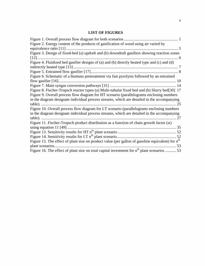
LIST OF FIGURES

Figure 1. Overall process flow diagram for both scenarios ...................................................... 1

Figure 2. Energy content of the products of gasification of wood using air varied by equivalence ratio [11] ............................................................................................................... 5

Figure 3. Design of fixed-bed (a) updraft and (b) downdraft gasifiers showing reaction zones [12] ............................................................................................................................................ 6

Figure 4. Fluidized bed gasifier designs of (a) and (b) directly heated type and (c) and (d) indirectly heated type [15] ........................................................................................................ 7

Figure 5. Entrained flow gasifier [17] ....................................................................................... 8

Figure 6. Schematic of a biomass pretreatment via fast pyrolysis followed by an entrained flow gasifier [16]..................................................................................................................... 10

Figure 7. Main syngas conversion pathways [31] .................................................................. 14

Figure 8. Fischer-Tropsch reactor types (a) Multi-tubular fixed bed and (b) Slurry bed[30] 17 Figure 9. Overall process flow diagram for HT scenario (parallelograms enclosing numbers in the diagram designate individual process streams, which are detailed in the accompanying table). ...................................................................................................................................... 25

Figure 10. Overall process flow diagram for LT scenario (parallelograms enclosing numbers in the diagram designate individual process streams, which are detailed in the accompanying table). ...................................................................................................................................... 27

Figure 11. Fischer-Tropsch product distribution as a function of chain growth factor (�) using equation 11 [49] ............................................................................................................ 35

Figure 13. Sensitivity results for HT nth plant scenario .......................................................... 52

Figure 14. Sensitivity results for LT nth plant scenario ........................................................... 52

Figure 15. The effect of plant size on product value (per gallon of gasoline equivalent) for nth plant scenarios ......................................................................................................................... 53

Figure 16. The effect of plant size on total capital investment for nth plant scenarios ........... 53

vi

LIST OF TABLES

Table 1. Reactions occurring within the reduction stage of gasification .................................. 5

Table 2. Previous techno-economic studies of biofuel production plants .............................. 19

Table 3. Process configurations considered in down selection process .................................. 20

Table 4. Main assumptions used in nth plant scenarios .......................................................... 23

Table 5. Stover and char elemental composition (wt%) ......................................................... 28

Table 6. Syngas composition (mole basis) for gasification scenarios evaluated .................... 30

Table 7. Fischer-Tropsch gas cleanliness requirements[30] ................................................... 33

Table 8. Hydroprocessing product distribution [50] ............................................................... 36

Table 9. Main economic assumptions for nth plant scenarios ................................................. 37

Table 10. Methodology for capital cost estimation for nth plant scenarios ............................. 39

Table 11. Variable operating cost parameters adjusted to 2007$ ........................................... 40

Table 12. Sensitivity parameters for nth plant scenarios ......................................................... 43

Table 13. Pioneer plant analysis parameters and factors ........................................................ 45

Table 14. Power generation and usage ................................................................................... 46

Table 15. Overall energy balance on LHV basis .................................................................... 47

Table 16. Overall carbon balance ........................................................................................... 48

Table 17. Capital investment breakdown for nth plant scenarios ........................................... 50

Table 18. Annual operating cost breakdown for nth plant scenarios ....................................... 51

Table 19. Catalyst replacement costs for both scenarios (3 year replacement period) ........... 51 Table 20. Pioneer Plant Analysis Results ............................................................................... 54

Table 21. Comparison of nth plant LT scenario to Tijmensen et al. study [41] ...................... 55

Table 22. Comparison of nth plant LT scenario to Larson et al. study [39] ............................ 56

Table 23. Main scenario nth plant results (TCI=total capital investment; TPEC=total purchased equipment cost; MM=million; GGE=gallon of gasoline equivalent) .................... 57

vii

ACKNOWLEDGEMENTS

Many of my friends and colleagues have helped and supported me along during my

research. I thank Dr. Brown for giving me the opportunity to join the Center for Sustainable

Environment Technologies (CSET) and perform this research. This opportunity allowed me

to discover and explore the exciting area of biorenewable resources. I would also like to

thank Dr. Anex in Agriculture and Biosystems Engineering and Dr. Meyer in Mechanical

Engineering for serving on my committee and providing guidance.

Moreover, I thank ConocoPhillips Company for the financial support of this research

and for providing the opportunity to further my learning during a summer visit to the

National Renewable Energy Laboratory. I thank Alex Platon of ConocoPhillips company for

imparting his expertise in support of this study.

I thank the National Renewable Energy Laboratory for allowing me the opportunity

to spend time at its laboratory where I was able to receive knowledge and expertise in

support of this study.

Behind the scenes, the administrative staffs of the Mechanical Engineering

department and CSET have supported me immensely by keeping things running smoothly. I

especially thank Diane Love, Becky Staedtler, and MaryAnn Sherman for frequent

assistance.

The talented scientists and fellow graduate students of CSET have provided much

guidance and feedback during meetings and presentations. I thank Justinus Satrio for his

frequent guidance throughout my research.

Finally, I thank my parents, Robert and Barbara Swanson for continual interest and

encouragement in my endeavors. Special thanks go to my good friends Cody Ellens and

Andy Herringshaw and my girlfriend Sara Hanenburg. Most of all, I thank God for the

talents he has bestowed upon me.

viii

ABSTRACT

This study compares capital and production costs of two biomass-to-liquid production

plants based on gasification. The goal is to produce liquid transportation fuels via Fischer-

Tropsch synthesis with electricity as co-product. The biorefineries are fed by 2000 metric

tons per day of corn stover. The first biorefinery scenario is an oxygen-fed, low temperature

(870°C), non-slagging, fluidized bed gasifier and the second scenario an oxygen-fed, high

temperature (1300°C), slagging, entrained flow gasifier. Both are followed by catalytic

Fischer-Tropsch synthesis and hydroprocessing to naphtha and distillate liquid fractions.

Process modeling software is utilized to organize the mass and energy streams and

cost estimation software is used to generate equipment costs. Economic analysis is

performed to estimate the capital investment and operating costs. A 20 year discounted cash

flow rate of return (DCFROR) analysis is developed to estimate a fuel product value (PV) at

a net present value of zero with 10% internal rate of return. All costs are adjusted to the year

2007.

Results show that the total capital investment required for nth plant scenarios are $610

million and $500 million, for high temperature and low temperature scenarios, respectively.

PV for the high temperature and low temperature scenarios are estimated to be $4.30 and

$4.80 per gallon of gasoline equivalent (GGE), respectively. The main reason for a

difference in PV between the scenarios is because of a higher carbon efficiency and

subsequent higher fuel yield for the high temperature scenario. Sensitivity analysis is also

performed on process and economic parameters which shows that total capital investment

and feedstock cost are among the most influential parameters affecting the PV while least

influential parameters include per pass Fischer-Tropsch reaction conversion extent, inlet

feedstock moisture, and catalyst cost.

In order to estimate the cost of a pioneer plant (1st of its kind) an analysis is

performed which inflates total capital investment and deflates the plant output for the first

several years of operation. Base case results of this analysis estimate a pioneer plant

investment to be $1.3 billion and $1.0 billion for high temperature and low temperature

scenarios, respectively. Resulting respective PV are estimated to be $7.40 and $7.70 per

GGE for pioneer plant.

1

1. INTRODUCTION

This study investigates economic feasibility of the thermochemical pathway of

gasification to renewable transportation fuels. The objective is to compare capital investment

costs and production costs for nth plant biorefinery scenarios based on gasification. The

selected scenarios are high temperature (slagging) gasification and low temperature (dry-ash)

gasification both followed by Fischer-Tropsch synthesis and hydroprocessing. They are

designed to produce liquid hydrocarbon fuels from 2000 dry metric ton (2205 dry short ton)

per day of agricultural residue, namely, corn stover.

The two scenarios were chosen from many options according to the following

criteria. The technology under consideration should be commercially ready in the next 5-8

years. The size of biorefinery should be feasible with current agricultural productivity and

within realistic feedstock collection area. In addition, the desired end product should be

compatible with the present fuel infrastructure, i.e. gasoline and/or diesel.

The high temperature gasification scenario is based on a steam/oxygen-fed entrained

flow, slagging gasifier similar to that described in Frey and Akunuri [1]. The low

temperature gasification scenario is based on a pressurized, steam/oxygen-fed fluidized bed

gasifier developed by Gas Technology Institute and reported by Bain [2]. The main areas of

operation are feedstock preprocessing, gasification, syngas cleaning, syngas

conditioning/upgrading, fuel synthesis, power generation, and air separation (for oxygen

production) as shown in Figure 1. Process modeling software is utilized to organize the mass

and energy streams and cost estimation software is used to generate equipment costs.

Economic analysis is performed to estimate the capital investment and operating costs. A 20

year discounted cash flow rate of return (DCFROR) analysis is developed to estimate a fuel

product value (PV) at a net present value of zero with 10% internal rate of return. All costs

are adjusted to the year 2007.

Figure 1. Overall process flow diagram for both scenarios

Dried

Biomass

Wet

Biomass

Raw

Syngas

Clean

Syngas

Raw

Fuel Fuel

SyngasOxygen

Power

Area 100:

Preprocessing

Area 200:

Gasification

Area 300:

Syngas

Cleaning

Area 400:

Fuel Synthesis

Area 700: Air Separation Unit Area 600: Power Generation

Area 500:

Hydroprocessing

2

2. BACKGROUND

The word economy is defined in the American Heritage Dictionary as “careful, thrifty

management of resources, such as money, material, or labor” and also as “an orderly,

functional arrangement of parts; an organized system.”[3] The origin of economy comes

from the Greek word oikonomiā meaning “the management of a household.”[3] Expanding

the word, it can be defined as the careful management of the all of the earth’s resources

including human beings, monetary systems, and, in regards to this study, energy.

Natural ecosystems are good examples of the earth’s economy in action. The earth’s

economy is evident in the aftermath of forest fires when new growth of forest rises from the

ashes. Certain species of conifers flourish the most after a fire because of the heat release of

seedlings. Another example is of the annual cycle of plant growth that humans use for

sustenance. Year after year the cycle continues as plants utilize the sun’s energy and the

soil’s nutrients to produce new crops. Continued energy from the sun and recycled nutrients

from decomposed plants keep the cycle moving. Observation of the earth’s cycles lead

humans to gain much knowledge of how to practice appropriate oikonomiā.

Over the past few decades it has become evident that the appropriate economy of the

earth’s carbon is important for the direction of human life. A study of history leads to the

realization that misuse of resources has serious consequences. During the middle of the last

millennium, European misuse of forests led to a near destruction of the forests and demanded

better resource management. The United States’ misuse of petroleum during the last century

led to the high point, or peak usage, of inexpensive, close-to-the-surface domestic petroleum.

The balance of energy dependence has now shifted to a high degree of instability. With

respect to appropriate oikonomiā, usage of carbonaceous energy resources requires careful

planning.

2.1 Biorenewable Resources

The world population has long utilized materials that are in close proximity. The

nearest resource available to the human population is the organic matter in the environment

around them. This organic matter is present for a limited amount of time due to its

decomposable nature. Brown [4] defines this material, or biorenewable resources, as organic

material of recent biological origin. It is a renewable resource if the rate of consumption is

3

equal to the regeneration or growth and therefore must be used only if preserving biodiversity

[5]. As a result, these resources have been important contributors to the world economy

serving as foodstuffs, transportation, energy, and construction materials, as well as many

other functions.

Biorenewable resources for generating energy can be classified as woody biomass,

energy crops, residues, and municipal waste [5]. The first two are primary resources while

the remaining are secondary resources meaning their primary use has already occurred.

Woody biomass includes logging products and energy crops include short rotation trees (e.g.

poplar) and switchgrass. Residues can come from logging processing or agricultural

processing (e.g. corn stover). According to Perlack et al. [6], the energy crop and agricultural

residue potential in the United States is 1.4 billion annual tons. According to Department of

Energy’s “Roadmap for Agriculture Biomass Feedstock Supply in the US,” there is potential

for 2 billion annual tons including municipal waste and biosolids (e.g. manure).

Many end products can be produced from these resources. Aside from the

conventional use of biomass for human food consumption, livestock feed, and building

materials, there are many new pathways to provide renewable alternatives to our

transportation, infrastructure, and energy. Combustion of biomass offers a way to provide

heat and power to displace coal and fuel oil. Liquefaction of biomass through fast pyrolysis

yields liquid products with the potential to displace petrochemicals. Additionally,

gasification of biomass allows for chemical and liquid fuel synthesis, which is the focus of

this study.

Developing an economy that involves biorenewable resources, especially biofuels,

has many benefits. According to Greene et al. [7], biofuel production has the potential to

provide a new source of revenue for farmers by generating $5 billion per year. Additionally,

air quality can be improved through the use of biofuels. In the same study Green et al.

reports that 22% of our total greenhouse gas emissions could be reduced if biofuels were

developed to replace half of our petroleum consumption. Arguably, the most important

benefit of biofuel production, when performed intelligently, is the potential for closing the

carbon cycle.

4

2.2 Gasification

Gasification is a high temperature and catalytic pathway to biofuels. It is defined as

the partial oxidation of solid, carbonaceous material with air, steam, or oxygen into a

flammable gas mixture called producer gas or synthesis gas [4]. The synthesis gas contains

mostly carbon monoxide and hydrogen with various amounts of carbon dioxide, water vapor,

and methane. Typical volumetric energy content of synthesis gas is between 4-18 MJ/Nm3

[8]. Comparatively, natural gas (comprised of mostly methane) energy content is 36 MJ/Nm3

[8]. Much of the energy content of the biomass is retained in the gas mixture by partial

oxidation rather than fully oxidizing the biomass which would result in the release of mostly

thermal energy. Historically, gasification of coal and wood produced “town gas” where it

was subsequently used to burn in street lamps [9]. Additionally, during the World Wars,

vehicles were adapted to operate with gasification reactors [9]. During this same time period

Germany developed the catalytic synthesis of transportation fuels from synthesis gas [10].

The same concept is still in use today by the South African Coal, Oil, and Gas Corporation

(SASOL) to produce motor fuels and liquid byproducts using coal [10].

2.2.1 Reaction

There are four stages that occur during gasification of carbonaceous material: drying,

devolatilization, combustion, and reduction [8]. First, the moisture within is heated and

removed through a drying process. Second, continued heating devolatilizes the material

where volatile matter exits the particle and comes into contact with the oxygen. Third,

combustion occurs where carbon dioxide and carbon monoxide are formed from carbon and

oxygen. The combustion stage is very exothermic and provides enough heat for the last stage,

the reduction reactions, to occur. The last stage includes water gas reaction, Boudouard

reaction, water-gas-shift reaction, and methanation reaction (Table 1). As all these stages

progress, solid fixed carbon remains present. Fixed carbon amount varies depending on the

equivalence ratio.

5

Table 1. Reactions occurring within the reduction stage of gasification

Name Reaction

Water gas � � ��� � �� � ��

Boudouard � � ��� � 2��

Water-gas-shift �� � ��� � ��� � ��

Methanation �� � 3�� � �� � ���

When equivalence ratio (defined as the actual air/fuel ratio all over the stoichiometric

air/fuel ratio) increases, solid fixed carbon (i.e. char) decreases until enough oxidizer is

available for complete conversion (Figure 2). This point of complete conversion occurs at

approximately 0.25 equivalence ratio. At nearly the same point, the maximum synthesis gas

energy content (without accounting for sensible energy) is reached.

Figure 2. Energy content of the products of gasification of wood using air varied by equivalence ratio

[11]

2.2.2 Gasifier Types

Gasification occurs in reactors of three types: fixed bed, fluidized bed, and entrained

flow [12]. Fixed beds are fed with biomass from the top of the reactor and form a bed which

0

5

10

15

20

25

0 0.1 0.2 0.3 0.4 0.5 0.6 0.7 0.8 0.9 1

enth

alp

y (M

J/kg

bio

mas

s, m

ois

ture

&as

h-f

ree)

equivalence ratio (mol/mol)

total

gas, total

gas, sensible heatgas, heating value

char, total

char, sensible heat

char, heating

value

6

gasifies as air moves through the bed (Figure 3). As the material releases volatile

components, the char and ash exit through a grate at the bottom. Typical operating

temperature range is 750-900°C. The two main types of fixed bed gasifiers are updraft and

downdraft. The advantage of fixed bed is simplicity, but is limited in scale up and has low

heat mixing due to high channeling potential within the reactor [13].

(a) (b)

Figure 3. Design of fixed-bed (a) updraft and (b) downdraft gasifiers showing reaction zones [12]

When the volumetric gas flow is increased through the grate the fixed bed becomes a

fluidized bed. Fluidized bed gasifiers are named because of the inert bed material that is

fluidized by oxidizing gas creating turbulence through the bed material (Figure 4). Biomass

enters just above top of the bed and mixes with hot, inert material creating very high heat and

mass transfer. Operating temperature range is the same as for the fixed bed. Advantages of

the fluidized bed include flexible feeds, uniform temperature distribution across bed, and

large volumetric flow capability [14]. The main types of fluidized bed gasifiers are

circulating fluidized bed (CFB) and bubbling fluidized bed, which are directly heated from

the combustion reactions occurring in the bed. A bubbling bed produces gas and the ash and

char falls out the bottom or the side. The CFB recycles the char through a cyclone while the

Biomass

Tars and

syngas

Ash

Air

Drying

Devolatilization

Reduction

Combustion

Biomass

Syngas

Ash

Air

Drying

Devolatilization

Reduction

Combustion

7

product leaves out the top of the cyclone. Indirectly heated fluidized beds use a hot material

such as sand to provide the heat needed for gasification as shown in Figure 4. Fluidized beds

have high carbon conversion efficiencies and can scale up easily [13].

(a) Bubbling fluidized-bed gasifier (b) Circulating fluidized-bed gasifier

(c) indirectly heated gasifier via combustor

(d) indirectly heated gasifier via heat exchange tubes

Figure 4. Fluidized bed gasifier designs of (a) and (b) directly heated type and (c) and (d) indirectly heated type [15]

Fluidized Bed

Steam/

Oxygen

BiomassAsh

Gasifie

r

Combustor

8

Another type of gasifier is the entrained flow gasifier (Figure 5). Normally operated

at elevated pressures (up to 50 bar) it requires very fine fuel particles gasified at high

temperatures to ensure complete gasification during the short residence times in the reactor.

The Energy Research Centre group of the Netherlands has investigated this gasification type

and have reported promise with biomass as long as the biomass is pretreated to certain

requirements [16]. To keep the residence time at approximately the time for a particle to fall

the length of the reaction zone, small fuel particles below 1 mm and high temperatures

(1100-1500°C) are necessary for successful operation.

Figure 5. Entrained flow gasifier [17]

Entrained flow gasification mixes the fuel with a steam/oxygen stream and forms into

a turbulent flow within the gasifier. Ash forming components melt in the gasifier and form a

liquid slag on the inside wall of the gasifier effectively protecting the wall itself. The liquid

flows down and is collected at the bottom. To form the slag, limestone can be added as a

fluxing material. For herbaceous biomass, such as switchgrass or corn stover, which is high

in alkali content, there may be sufficient inherent fluxing material present [17]. Advantages

9

of entrained flow gasification are that tar and methane content are negligible and high carbon

conversion occurs due to more complete gasification of the char. Syngas clean up is

simplified because slag is removed at the bottom of the gasifier negating the need for

cyclones and tar removal [18]. The disadvantages are that very high temperatures need to be

maintained and the design and operation is more complex. An entrained flow gasifier co-

firing up to 25% biomass with coal has been developed by Shell in Buggenum, Netherlands.

Another gasifier developed by Future Energy in Freiburg, Germany uses waste oil and

sludges. Both are operating at commercial scale [16].

2.3 Biomass Preprocessing

A degree of processing is required before gasification can occur. Most gasifiers

require smaller size feedstock than is typically collected during harvest. Therefore, a

significant degree of size reduction needs to be performed. A typical setup for size reduction

is using a two-step process where a chipper accomplishes the primary reduction followed by

a hammer mill for the secondary reduction [19]. In addition, a maximum moisture content for

gasification is between 20-30% (wet basis) and normal operation is less than 15% (wet basis)

[8]. Therefore, a drying process is required to prepare the feedstock for gasification.

The main benefit of drying biomass is to avoid using energy within the gasifier to

heat and dry the feedstock [20]. Drier biomass makes for more stable temperature control

within the gasifier. Rotary dryers typically operate utilizing hot flue gas from a downstream

process as the drying medium. They have high capacity, but require high residence times. In

addition, rotary dryers have a high fire hazard when using flue gas [20]. To avoid using flue

gas, rotary dryers can use superheated steam, essentially an inert gas, when a combined cycle

heat and power system is used downstream. That system has significant steam available for

use because of the steam produced in the steam cycle. An advantage of using steam for

drying is better heat transfer and therefore shorter residence time.

Pretreatment options for entrained flow gasification include torrefaction followed by

grinding to 0.1 mm particles, grinding to 1 mm particles, pyrolysis to produce bio-oil/char

slurry (bioslurry), or initial fluidized bed gasification of larger particles coupled to an

entrained flow gasifier. Torrefaction, essentially an oxygen-free roasting process, causes the

biomass particles to be brittle for easy grinding, but releases up to 15% of the energy in the

biomass via volatile compounds

energy efficiency of 80-85%, but is expensive due to the

bio-slurry option is illustrated

and char followed by a slagging, entrained flow gasifier.

entrained flow gasifier, the feed must be press

already in an emulsified liquid state, can be pressurized

feeding is state of the art due to experience with coal slurries

contains 90% of the energy contained in the

no inert gas is needed for solids pressurization,

dilute the syngas. In the search for cost effective methods for production of syngas, this

option has potential, but isn’t as developed as technologies such as fluidized bed gas

The biggest challenge is constructing and operating a large

large-scale systems have not been demonstrated

Figure 6. Schematic of a biomass pretreatment via fast pyrolysis followed by an entrained flow

2.4 Syngas Cleaning

Since the raw syngas leaving the gasifier cont

sulfur compounds, nitrogen compounds, and other contaminants, those components must be

removed or reduced significantly. Particulate and tars have the potential for clogging

downstream processes. Sulfur and nitroge

processes especially catalysts used in fuel synthesis applications. Moreover, another

motivation to clean syngas is meeting environmental emissions limits.

biomass via volatile compounds [16]. The coupled option is attractive because of an overall

85%, but is expensive due to the two gasifiers used in series.

option is illustrated in Figure 6. Basically, a flash pyrolysis process yields bio

and char followed by a slagging, entrained flow gasifier. Since this process utilizes an

feed must be pressurized. Fortunately, the pyrolysis slurry,

liquid state, can be pressurized easily. Technology for slurry

due to experience with coal slurries [16]. The bioslurry still

contains 90% of the energy contained in the original biomass [21]. Another advantage is that

for solids pressurization, which would dilute the feed and therefore

In the search for cost effective methods for production of syngas, this

option has potential, but isn’t as developed as technologies such as fluidized bed gas

The biggest challenge is constructing and operating a large-scale pyrolysis process

scale systems have not been demonstrated [16].

. Schematic of a biomass pretreatment via fast pyrolysis followed by an entrained flow gasifier [16].

Since the raw syngas leaving the gasifier contains particulate, tars, alkali compounds,

sulfur compounds, nitrogen compounds, and other contaminants, those components must be

removed or reduced significantly. Particulate and tars have the potential for clogging

downstream processes. Sulfur and nitrogen have the potential to poison downstream

processes especially catalysts used in fuel synthesis applications. Moreover, another

motivation to clean syngas is meeting environmental emissions limits.

10

. The coupled option is attractive because of an overall

two gasifiers used in series. The

. Basically, a flash pyrolysis process yields bio-oil

Since this process utilizes an

urized. Fortunately, the pyrolysis slurry,

echnology for slurry

lurry still

. Another advantage is that

which would dilute the feed and therefore

In the search for cost effective methods for production of syngas, this

option has potential, but isn’t as developed as technologies such as fluidized bed gasification.

scale pyrolysis process since

. Schematic of a biomass pretreatment via fast pyrolysis followed by an entrained flow

ains particulate, tars, alkali compounds,

sulfur compounds, nitrogen compounds, and other contaminants, those components must be

removed or reduced significantly. Particulate and tars have the potential for clogging

n have the potential to poison downstream

processes especially catalysts used in fuel synthesis applications. Moreover, another

11

Cooling of the syngas must occur before conventional gas clean up is to be utilized.

This can happen two ways: direct quench by injection of water and indirect quench via a heat

exchanger. Direct quench is less expensive, but dilutes the syngas. The direct quenching also

can be used to clean up the gas by removing alkali species, particulate, and tars [22].

Particulate is defined as inorganic mineral material, ash, and unconverted biomass, or

char [23]. In addition, bed material from the gasifier is included in the particulate. For

feedstock such as switchgrass typically has 10% inorganic material in the form of minerals.

Many gasifiers operate with a 98-99% carbon conversion efficiency where 1-2% of the solid

carbon is in the form of char [23].

Removal of particulate primarily occurs through physical methods like cyclones

where the heavy particles fall down the center while the gases rise up and out of the cyclone.

The initial step for particulate removal is usually a cyclone. Important in particulate removal

is that they should be removed before the gas is cooled down for cold gas cleaning. If

removed after gas cooling, then tars can condense onto particulate and potentially plug

equipment. Barrier filters, which operate above tar condensation temperatures use metal or

ceramic screens or filters to remove particulate allow the gas to remain hot, but have

presented problems in sintering and breaking [23].

Even more critical to downstream syngas applications is tar removal. Tars are

defined as higher weight organics, oxygenated aromatics, heavier than benzene 78 and are

produced from volatized material after polymerization [23]. A review by Milne et al. [24] of

tars produced during gasification covers different removal methods. Physical removal via wet

gas scrubbing of tars is accomplished by a scrubbing tower for the “heavy tars” followed by a

venturi scrubber for lighter tars. This setup is similar to the direct quench cooling as

mentioned previously since cooling occurs as well. Tar concentration is reported to be lower

than 10 ppm by volume at the exit of this setup. The disadvantage of this setup is that waste

water treatment is required and can be expensive. The other method for tar removal is

catalytic or thermal conversion to non-condensable gas. This is also known as hot gas

cleaning since it occurs at temperatures at or above gasification temperatures. Catalytic

conversion can occur as low as 800 °C and thermal conversion occur up to 1200 C. The

12

energy required for thermal tar cracking may not be cost competitive because of the

temperature rise from the gasification temperature to crack the high refractory tars [23].

Alkali compounds such as calcium oxide and potassium oxide are present in biomass

and when gasified either become vaporized or concentrated in the ash. Condensation of

these compounds begins at 650°C and can deposit on cool surfaces causing equipment

clogging, equipment corrosion, and catalyst deactivation [25]. According to Stevens [25],

research on alkali adsorption filters using bauxite has been promising, but not demonstrated

on a large scale. Stevens concludes that the best current method for alkali removal is using

proven syngas cooling followed by wet scrubbing, where the addition of water cools the

syngas and physically removes small particles and liquid droplets.

Wet scrubbing also removes ammonia which forms during gasification from the

nitrogen in the biomass. Without proper removal, ammonia can deactivate catalysts as well.

Complete ammonia removal can be accomplished through wet scrubbing [26]. For gasifiers

coupled to a catalytic or thermal tar reformer, most of the ammonia can be reformed to

hydrogen and nitrogen [26]. Sulfur in the biomass mostly forms into hydrogen sulfide (H2S)

with small amounts of carbonyl sulfide (COS). Hydrogen sulfide removal occurs by three

main ways: chemical solvents, physical solvents, and catalytic sorbents. For chemical

removal, amine-based solvents are typically utilized. Chemical removal occurs by the

solvent chemically bonding with H2S. Physical removal takes advantage of the high

solubility of H2S using an organic solvent. Typical setups of both chemical and physical

removal involve an absorber unit followed by a solvent regenerator unit, known as a stripper.

Operation usually occurs at temperatures lower than 100°C and medium to high pressures

(150-500 psi) [26]. Sulfur leaving these two systems is around 1-4 ppm and can require

further removal, especially for fuel synthesis. In that case, a syngas polishing step using a

fixed bed zinc oxide activated carbon catalyst removes H2S and COS to parts per billion

levels necessary for fuel synthesis. Halides, present in trace amounts in the biomass, can also

be removed with the zinc oxide catalyst [26].

2.5 End Use Product

After syngas has been cleaned from particulates, impurities, and contaminants there is

sufficient energy content for producing a higher valued product. There are three main large-

13

scale biomass gasification pathways that have been researched and suggested for higher

valued product: power generation, liquid fuel synthesis, and chemical synthesis. According

to Wender [27], the three largest commercial uses for syngas are ammonia production from

hydrogen, methanol synthesis, and hydrocarbon synthesis via Fischer-Tropsch process.

2.5.1 Power Generation

Power generation using gasification occurs by combusting the syngas in a gas turbine

to provide mechanical work for a generator. Steam is generated by recovering heat from the

hot syngas and the steam in turn provides the means for mechanical work via a steam turbine.

This gasifier plus gas and steam turbine setup is known as integrated gasification combined

cycle (IGCC) power generation. The level of particulates, alkali metals, and tar can decrease

the performance of the gas turbine. Consonni and Larson [28] found that particulate can

cause turbine blade erosion and 99% of 10 micron size particles or less should be removed.

In addition, they also report that alkali metals corrode the turbine blades and tars condense on

the turbine blades both hindering operation and escalating turbine failure. Fortunately, nearly

all alkali and tars can be removed using proven wet scrubbing techniques.

Using the IGCC approach to generate power, Bridgwater et al. [29] and Craig and

Mann [22] expect biomass to power efficiencies in the range of 35-40% with large scale

systems (greater than 100 MW net output) at the high end of the range. Moreover, Craig and

Mann suggest that future advanced turbine systems could reach 50% biomass to power

efficiency.

2.5.2 Synthetic Fuels and Chemicals

Instead of converting the energy content of the syngas to power, the energy content

can be condensed into a liquid energy carrier, or fuel. The conversion of syngas to fuels can

only occur in the presence of proper catalysts [30]. The catalytic reactions basically build up

the small molecules in the syngas (i.e. carbon monoxide and hydrogen) into larger

compounds that are more easily stored and transported. A summary of many catalytic

pathways to fuels and chemicals is shown in Figure 7. In most catalytic synthesis reactions,

syngas cleanliness requirements are very high. Most impurities and contaminants are

removed to low parts per million and even parts per billion. This means that significant cost

must be directed towards syngas cleaning.

Figure

2.5.2.1 Methanol to Gasoline Methanol is one of the top chemicals produced in the world

produced methanol is synthesized via steam methane reforming and autothermal reforming.

The synthesis of methanol from syngas is highly exothermic (equation 1). The reaction

occurs over a Cu/ZnO/Al2O3

50-100 bar and have lifetime of 2

conversion efficiency can reach 99% with recycle, but per pass efficiency is about 25%.

Although methanol can be used directly as a liquid fuel, it can

the conventional transportation fuel range. This process is known as the methanol

gasoline (MTG) process and

removed to low parts per million and even parts per billion. This means that significant cost

must be directed towards syngas cleaning.

gure 7. Main syngas conversion pathways [31]

hanol to Gasoline Methanol is one of the top chemicals produced in the world [31]. Most commercially

produced methanol is synthesized via steam methane reforming and autothermal reforming.

The synthesis of methanol from syngas is highly exothermic (equation 1). The reaction

catalyst between temperatures of 220-275°C and pressures of

100 bar and have lifetime of 2-5 years [30]. Wender [27] reports syngas to methanol

each 99% with recycle, but per pass efficiency is about 25%.

methanol can be used directly as a liquid fuel, it can also be converted into

the conventional transportation fuel range. This process is known as the methanol

nd was developed by the Mobil Oil Corporation [30]

14

removed to low parts per million and even parts per billion. This means that significant cost

. Most commercially

produced methanol is synthesized via steam methane reforming and autothermal reforming.

The synthesis of methanol from syngas is highly exothermic (equation 1). The reaction

275°C and pressures of

syngas to methanol

each 99% with recycle, but per pass efficiency is about 25%.

(eqn. 1)

be converted into

the conventional transportation fuel range. This process is known as the methanol to

[30]. In that

15

process, methanol is heated to 300°C and dehydrated over alumina catalyst at 27 atm

yielding methanol, dimethyl ether (DME), and water. The exiting mixture reacts with a

zeolite catalyst at 350°C and 20 atm to produce 56% water and 44% hydrocarbons by weight.

Of the hydrocarbon product, 85% is in the gasoline range and 40% of the gasoline range is

aromatic. However, limitations on the aromatic content of gasoline have been proposed in

legislation [30]. Thermal efficiency of methanol to gasoline range hydrocarbons is 70% [10].

The overall MTG process usually contains multiple MTG reactors in parallel in order to

perform periodic catalyst regeneration by burning off coke deposits [10]. A commercial

plant producing 14,500 barrels per day operated in New Zealand during the 1980s by Mobil

[31]. The reaction process could stop directly after the methanol synthesis and focus on

producing DME because it can be used as a diesel fuel as it has a high cetane number. It is

formed from the dehydration reaction of methanol over an acid catalyst γ-alumina. Per pass

can be as high at 50%. Overall syngas to DME is higher than syngas to methanol [30].

However, DME is in gaseous form at atmospheric conditions and needs to be pressurized for

use in diesel engine [32]. Therefore, engine modification is required and is the main

disadvantage for DME use as transportation fuel.

2.5.2.2 Fischer-Tropsch Fischer-Tropsch catalytic synthesis is a highly exothermic reaction producing wide

variety of alkanes (equation 2).

�� � 2.1�� � ������ � � ��� (eqn. 2)

For gasoline range products, higher temperatures (300-350°C) and iron catalysts are

typically used. For diesel range and wax products, lower temperatures (200-240°C) and

cobalt catalysts are typically used [33]. Operating pressures are in the range of 10-40 bar.

Product distribution can be estimated using the Anderson-Schulz-Flory chain growth

probability model where longer hydrocarbon chains form as the temperature decreases. At

high temperatures, selectivity favors methane and light gases. This is a disadvantage if liquid

fuel production is the focus. At low temperatures, selectivity favors long carbon chain wax

products requiring further hydrocracking to the diesel range in a separate unit adding more

construction cost, but necessary for liquid fuel production.

16

Because of the highly exothermic reaction, the heat must be removed or the catalyst

can be deactivated. Two main types of reactors have been designed: a fixed bed tubular

reactor and slurry phase reactor (Figure 8). Heat removal is crucial to the process and has

been the focus of reactor design development [30]. The fixed bed reactor has many catalyst

tubes where heat removal is achieved by steam generation on the outside of the tubes [34].

The fixed bed reactor is simple to operate and is well suited for wax production due to simple

liquid/wax removal. However, it is more expensive to build because of the many tubes and

has a high pressure drop across the reactor [35]. The slurry phase reactor (SPR) operates by

suspending catalyst in a liquid and the syngas is bubbled through from the bottom. A

disadvantage of a SPR is a more complex operation and difficult wax removal. However, the

SPR requires approximately 40% less construction cost [35].

FT diesel is very low in sulfur, low in aromatic content, and has high cetane number,

making it very attractive as conventional fuel alternative. Emissions across the board

decrease when using FT diesel. A South African based company, Sasol, has been producing

transportation fuel since 1955 using the FT process and supplies 41% of South Africa’s

transportation fuel requirements [30].

17

(a) (b)

Figure 8. Fischer-Tropsch reactor types (a) Multi-tubular fixed bed and (b) Slurry bed[30]

2.6 Techno-economic Analysis

In order for biofuels technologies to be utilized in commercial applications, the

economic feasibility must be determined. A feasibility analysis is also called a techno-

economic analysis where the technical aspects of a project are coupled to the economic

aspects. First, the basic theoretical configuration is developed and a mass and energy balance

is performed. Second, cost estimation allows the investment and production cost of a

biorefinery to be determined. With rising interest in biorenewable resources, many techno-

economic studies have been performed on power generation and biofuel scenarios. These

studies assist in understanding how the physical process relates to cost of producing

renewable alternatives. Accuracy of results from these studies is usually ±30% of the actual

cost [4].

2.6.1 Economics of Biomass Power

A study by Bridgwater in 1994 [36] demonstrated that an IGCC power generation

plant using biomass at 100 MW electric output could produce power for 6 ¢ per kWh and

18

would require $2000 per kW (i.e. $200 million total) in capital investment. That study also

compared between various power generation pathways showing that an IGCC could produce

power for less compared to combustion and gas engine scenarios. Another study by Craig

and Mann [22] using 1990$ compares varying IGCC scenarios with power output between

56-132 MW. Capital investment for these scenarios range between $1100 to 1700 per kW

and production cost of power range between 6.5 and 8.2 ¢ per kWh. A study by Larson et al.

[37] increases the power generation to 440 MW and shows that the increased size benefits

from economies of scale. Capital investment is $1000 per kW and production cost of power

is just above 5¢ per kWh.

2.6.2 Economics of Biofuels

Previous studies of gasification based, biomass-to-liquid production plants have

estimated the cost of transportation fuels to range from $12-16/GJ ($1.60-2.00 per gallon of

gasoline equivalent) [15,38-41]. The same studies have estimated total capital investment in

the range of $191 million for 2000 dry metric ton per day input [40] to $541 million for 4500

dry metric ton per day input [39].

A 1650 dry metric ton per day biomass to methanol plant based on gasification,

production cost of $15/GJ ($0.90 per gallon of methanol) is reported by Williams et al. [15]

in 1991$ for $45 per dry metric ton of biomass. Williams et al. also shows production cost of

methanol derived natural gas to be $10/GJ ($0.60 per gallon of methanol). However, that

study concludes that if a carbon tax system was developed for lifecycle carbon emissions,

then renewable methanol could become competitive to natural gas derived methanol at a tax

of approximately $90 per metric ton of carbon. A more recent study by Larson et al. of

switchgrass to hydrocarbons production in 2009 reports a production cost of $15.3/GJ ($1.90

per gallon of gasoline) in 2003$ for a 4540 dry metric ton per day (5000 dry short ton per

day) plant based on gasification [39].

Table 2 shows a comparison between four biofuel production studies based on

gasification. A range of cost year, plant size, and feedstock cost show the diversity of

characteristics and assumptions that techno-economic studies use. In addition, resulting

capital investment costs of the studies have a large range. For example, the capital

investment of the Phillips et al. and Tijmensen et al. studies are $191 million and $387

19

million, respectively, at similar plant sizes. Reasons for such a significant difference are

choice of technologies and level of technology development. The Phillips et al. study is a

target study meaning that it estimates future technology improvement and results in lower

costs. Direct comparison is difficult because of the varying assumptions used by each study.

Table 2. Previous techno-economic studies of biofuel production plants

Williams et al. [15]

Phillips et al. [40]

Tijmensen et al. [41]

Larson et al. [39]

Cost Year 1991 2005 2000 2003

Plant Size (dry metric tonne per day)

1650 2000 1741 4540

Feedstock generic biomass

poplar poplar switchgrass

Fuel Output methanol ethanol FT liquids diesel, gasoline

Feedstock Cost ($/dry short ton)

41 35 33 46

Capital Investment ($MM)

N/A 191 387 541

Product Value ($/GJ) 15 12 16 15

Product Value ($/GGE) 1.90 1.60 2.00 1.85

20

3. METHODOLOGY

The following steps are undertaken to perform the analysis in this study:

• Collect performance information on relevant technologies for systems under evaluation.

• Perform down selection process with developed criteria to identify most appropriate scenarios

• Design process models using Aspen PLUSTM process engineering software • Size and cost equipment using Aspen Icarus Process Evaluator®, literature

references, and experimental data • Determine capital investments and perform discounted cash flow analysis • Perform sensitivity analysis on process and economic parameters • Perform pioneer plant cost growth and performance analysis

3.1 Down Selection Process

A number of process configurations for the gasification-based, biomass to liquids

(BTL) route are initially considered as listed in Table 3 and discussed in the following

sections.

Table 3. Process configurations considered in down selection process

Gasifier block

Entrained flow, slagging gasifier

Fluid bed, dry ash gasifier

Transport gasifier, dry ash (e.g. Kellog, Brown, and Root)

Indirect gasifier, dry ash (e.g. Battelle-Columbus Labs)

Syngas cleaning

Water scrubbing

Catalytic tar conversion/reduction

Thermal tar conversion/reduction

Amine-based acid gas removal

Physical sorbent-based acid gas removal (e.g. Sorbitol, Rectisol)

Fuel synthesis

Fischer-Tropsch

Mixed alcohols

Methanol to gasoline (MTG)

Dimethyl ether

Syngas fermentation

21

3.1.1 Preliminary Criteria

The initial technology configuration options are reviewed and screened in accordance

with the following criteria. The technology under consideration should be commercially

ready in the next 5-8 years and preferably with high technology development. High

technology development increases the likelihood of a configuration to perform at the scale in

this study. For example, coal gasification has been demonstrated commercially at large-

scales [10]. While similar scale biomass gasifiers have not been proven commercially, the

technology development on coal is assumed to apply for biomass in 5-8 years. Secondly, the

size of biorefinery should be feasible with typical agricultural productivity and within a

realistic collection area. For example, if one third of total land use surrounding the

biorefinery is for stover collection and each acre provides conservatively one short dry ton

per year, then the required collection radius is 35 miles and amount of biomass transported to

the biofinery is approximately 2300 short tons (2090 metric tons) per day. The collection

area with a 35 mile radius is assumed to be realistic. In addition, previous studies by

Tijmensen et al., Phillips et al., and Lau et al. have used a similar plant sizes [40-42]. Thirdly,

the desired product should be compatible with the present transportation fuel infrastructure,

i.e. gasoline and diesel range hydrocarbons.

3.1.2 Scenarios selection

For the gasification area, two gasifiers were selected for modeling. First, an entrained

flow, slagging gasifier is chosen due to its commercial application with coal (GE, Siemens,

Shell, and ConocoPhillips) and its potential for use with biomass. Moreover, process

modeling of this gasifier is simple since it can be closely approximated at thermodynamic

equilibrium [1]. Second, a fluidized bed, dry ash gasifier is chosen due to experience at Gas

Technology Institute and because of data availability. A report by Bain [2] at the National

Renewable Energy Laboratory contains collected and analyzed data for fluidized bed

gasification. In addition, Iowa State University is currently operating an atmospheric

pressure, fluidized bed gasifier as either air or oxygen/steam fed.

The syngas cleaning area is chosen to include configurations that have less

technological complexity than previous studies. Phillips et al. [40] and Larson et al. [39]

both employ an external catalytic tar reforming process for dry-ash gasification. Because of

22

low technological development in tar conversion and its inherent complexity, a direct-contact

syngas quenching and scrubbing are chosen for this study. In the case of the slagging

gasifier, high temperatures inhibit tar formation, yet still require quenching and particulate

and ammonia removal. An amine-based, chemical absorber/stripper configuration is chosen

for removal of hydrogen sulfide and carbon dioxide. This configuration is chosen due to data

availability as compared to proprietary physical gas cleaning process such as Rectisol® and

Selexol®.

Two fuel synthesis configurations under consideration produce liquid hydrocarbons:

Fischer-Tropsch (FT) synthesis and MTG. FT synthesis has been proven in operation at

commercial scale for many years by Sasol [10]. Due to more accessible data and long

industrial experience, FT synthesis is the only fuel synthesis option chosen. A consequence

of this selection is a post-synthesis fuel upgrading area since FT products need to be

separated and hydroprocessed.

3.1.3 Scenarios not selected

The indirect, dry-ash gasifier and the mixed alcohol synthesis configurations is not

considered due to previous work by Phillips et al. [40] The transport gasifier design, though

a promising technology, is not considered due to reactor complexity, unproven commercial-

scale operation and lack of public domain data. Tar conversion via external thermal or

catalytic cracking is not considered due to lack of public domain data and commercial scale

experience. Acid gas removal using proprietary technology (e.g. Rectisol™ or Selexol™) is

not considered because of a lack of public operational data. MTG, including methanol

synthesis, is not considered because of time constraints and limited operational data. DME

and syngas fermentation is not considered due to the limited commercial scale experience

and because of incompatibility with present fuel infrastructure.

3.1.4 Project Assumptions

Main project assumptions for process and economic analysis are listed in Table 4. A

more extensive list can be found in Appendix A.

23

Table 4. Main assumptions used in nth plant scenarios

Main assumptions

The plant is modeled as nth plant

Plant capacity is 2000 dry metric ton/day

Feedstock is corn stover at 25% moisture

Feedstock ash content at 6%

Feedstock is purchased at plant gate for $75/dry short ton

All financial values are adjusted to 2007 cost year

Plant is 100% equity financed

Fuel PV is evaluated at 10% internal rate of return

Plant initiates operation in 5-8 year time frame

Plant life is 20 years

Plant availability is 310 days per year (85%)

3.2 Process Description

3.2.1 High Temperature Scenario Overview

The high temperature scenario is a 2000 dry metric ton (2205 dry short ton) per day

corn stover-fed gasification biorefinery that produces naphtha and distillate to be used as

blendstock as well as electricity for export. It is based on pressurized, oxygen blown,

entrained flow gasification. The HT scenario is an nth plant design meaning significant

design, engineering, and operating experience has been achieved.

The main areas of operation as shown in Figure 9 include feedstock preprocessing

(Area 100) where the stover is chopped, dried, and ground to 1-mm, 10% moisture.

Gasification (Area 200) contains the stover pressurization for solids feeding, gasification, and

slag removal. Synthesis gas cleaning (Area 300) contains cold gas cleaning technologies

where the syngas is quenched and scrubbed from particulate, ammonia, hydrogen sulfide,

and carbon dioxide. Area 300 also contains the water-gas-shift reaction which occurs before

the hydrogen sulfide and carbon dioxide removal in order to adjust the ratio of hydrogen to

carbon monoxide for optimal fuel synthesis. Fuel synthesis section (Area 400) contains

syngas boost pressurization, contaminant polishing via zinc oxide guard beds, Fischer-

Tropsch reactor, and hydrocarbon gas/liquid separation. Hydroprocessing (Area 500)

produces the final fuel blend and is treated as a black box utilizing published data. Power

generation (Area 600) contains gas and steam turbines along with a heat recovery steam

generator. Area 700 contains the Air Separation Unit (ASU) where oxygen is separated from

24

air and pressurized for use in the gasifier. For cost analysis uses only, a balance of plant

(BOP) area accounts for cooling tower area, cooling water system, waste solids and liquids

handling area, and feed water system. Detailed process flow diagrams can be found in

Appendix E and detailed stream data can be found in Appendix F.

Recycle streams are utilized to provide better syngas to FT products conversion.

Unconverted syngas in the fuel synthesis area is recycled to the syngas cleaning area to

remove carbon dioxide and allows for further conversion in the Fischer-Tropsch reactor. A

small portion of unconverted syngas is sent to a steam boiler to raise steam required for

drying the biomass. The balance of unconverted syngas is combusted in a gas turbine and

waste heat is recovered in a steam generator for steam turbine power. Power generated is

used throughout the plant and excess is sold.

Some of the largest consumers of power are the ASU and hydroprocessing area at

11.6 MW and 2.2 MW, respectively. Another consumer of power is the hammermill for

grinding the dried biomass in Area 100 requiring 3.0 MW. The amine/water solution

recirculation pump in Area 300 requires approximately 0.9 MW. Syngas compressors

throughout the plant require significant amount of power as well. Gross plant power

production is 48.6 MW and net electricity for export is 13.8 MW.

25

Figure 9. Overall process flow diagram for HT scenario (parallelograms enclosing numbers in the

diagram designate individual process streams, which are detailed in the accompanying table).

3.2.2 Low Temperature Scenario Overview

The low temperature scenario is a 2000 dry metric ton (2205 dry short ton) per day

corn stover-fed gasification biorefinery that produces naphtha and distillate to be used as

blendstock as well as electricity for export. It is based on a pressurized, oxygen/steam blown

fluidized bed gasifier developed by Gas Technology Institute. The HT scenario is an nth

plant design meaning significant design, engineering, and operating experience has been

achieved.

The main areas of operation as shown in Figure 10 include feedstock preprocessing

(Area 100) where the stover is chopped, dried, and ground to 6-mm, 10% moisture.

Gasification (Area 200) contains the stover pressurization for solids feeding, gasification, and

char and ash removal. Synthesis gas cleaning (Area 300) contains cold gas cleaning

technologies where the syngas is quenched and scrubbed from particulate, ammonia,

hydrogen sulfide, and carbon dioxide. Fuel synthesis section (Area 400) contains syngas

Dryer

Acid Gas

Removal

Water,

Solids

Fischer

TropschHydroprocessing

Naphtha, Distillate

to storage

Fuel Gas

to A600

Slag

Grinder Entrained

Flow

Gasifier

Lockhopper

Water

Sour Water

Gas Shift

LO-CAT

Sulfur

Cake

Compressor

Pressure Swing

Adsorption

Hydrogen

Power

Combustion

Flue Gas

Steam

Syngas

A700

A100

A200 A300 A400 A500

A600Chopper

Power Generation

SteamStover

Air

Condensate

Nitrogen

Oxygen

Dry Stover

Syngas

Carbon Dioxide

1

2

3

4

5

6

7

8

9

10

11

12

13

14

15

16

17

18

19

20

21

22

24

23

25

2627

28

29

33

Oil/Water

Separation

Water34

31

32

30

Direct Quench

Stream 1 2 3 4 5 6 7 8 9 10 11 12 13 14 15 16 17T (°C) 25 25 90 90 16 32 149 120 200 120 220 249 1300 50 203 203 190P (bar) 1.01 1.01 1.01 1.01 1.1 1.01 28 1.98 1.98 1.98 1.03 28 26.62 26.62 26.62 25.93 10m (Mg/day) 2667 2667 2222 2222 2189 2903 744 444 4000 4000 271 180 3823 114 4000 3867 550Stream 18 19 20 21 22 23 24 25 26 27 28 29 30 31 32 33 34T (°C) 240 40 40 50 50 62 76 30 200 42 45 45 45 35 35 35 37P (bar) 24.8 24.82 24.82 3.45 1.93 22.75 26 1.01 24.96 23.6 23.58 23.58 23.58 22.2 22.2 22.2 1.03m (Mg/day) 4417 1502 2965 1755 3.1 3570 3570 4.38 1404 1068 2308 156 33 427 641 52 378

26

boost pressurization, contaminant polishing via zinc oxide beds, Fischer-Tropsch reactor, and

hydrocarbon gas/liquid separation. Also included within area 400 is the steam methane

reformer (SMR) to reduce methane content and water-gas-shift (WGS) to adjust ratio of

hydrogen and carbon monoxide. Hydroprocessing (Area 500) produces the final fuel blend

and is treated as a black box utilizing published data. Power generation (Area 600) contains

gas and steam turbines along with a heat recovery steam generator. Area 700 contains the

Air Separation Unit (ASU) whereby oxygen is separated from air and pressurized for use in

the gasifier. Detailed process flow diagrams can be found in Appendix E and detailed stream

data can be found in Appendix F.

Recycle streams are utilized to provide better FT products conversion. Unconverted

syngas in the fuel synthesis area is recycled to the syngas cleaning area to remove carbon

dioxide and allows for further conversion in the Fischer-Tropsch reactor. The balance of

unconverted syngas is combusted in a gas turbine and waste heat is recovered in a steam

generator for steam turbine power. Power generated is used throughout the plant and excess

is sold. Unconverted carbon within the gasifier in the form of char is collected and

combusted in a furnace to produce heat thereby generating steam for the drying of the

biomass.

Some of the largest consumers of power are the ASU and hydroprocessing area at 9.1

MW and 1.7 MW, respectively. Another consumer of power is the hammermill for grinding

the dried biomass in Area 100 requiring 1.1 MW. The amine/water solution recirculation

pump in Area 300 requires approximately 0.7 MW. Syngas compressors throughout the

plant require a significant amount of power as well. Gross plant power production is 40.7

MW and net electricity for export is 16.3 MW.

27

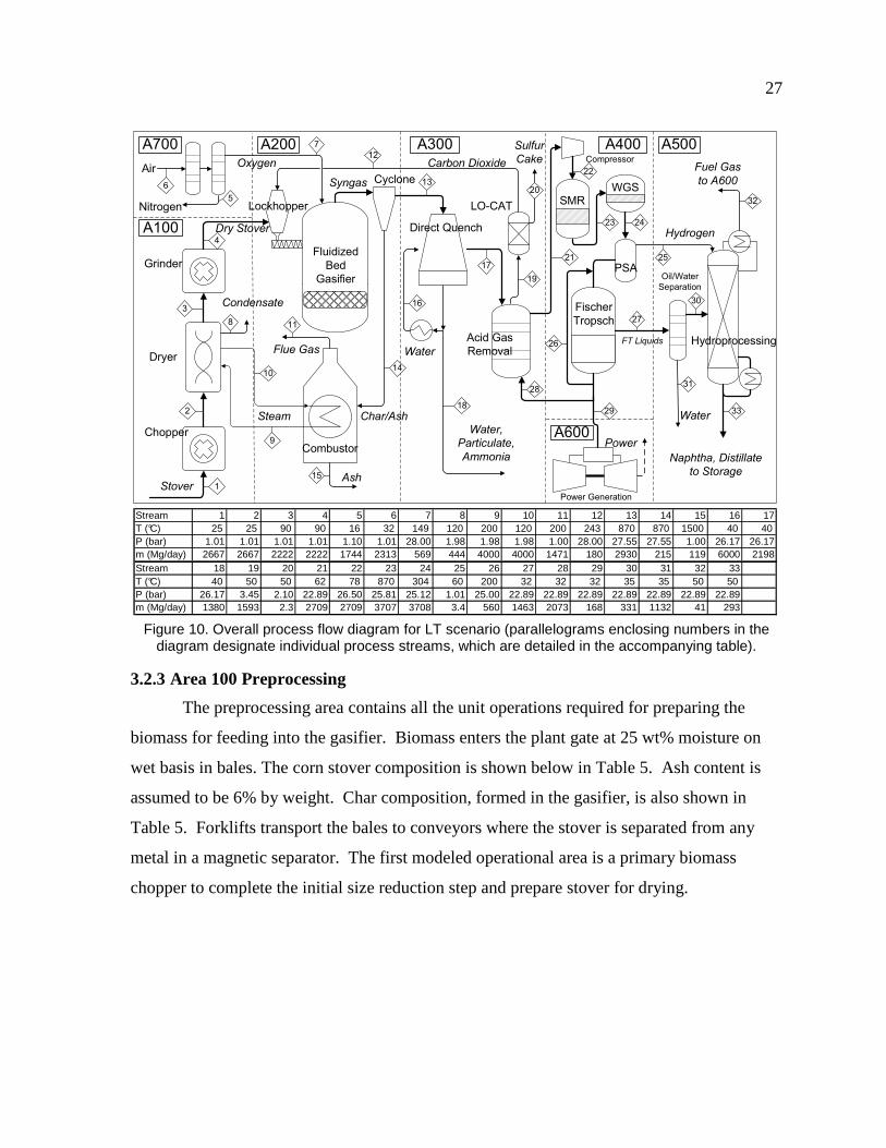
Figure 10. Overall process flow diagram for LT scenario (parallelograms enclosing numbers in the

diagram designate individual process streams, which are detailed in the accompanying table).

3.2.3 Area 100 Preprocessing

The preprocessing area contains all the unit operations required for preparing the

biomass for feeding into the gasifier. Biomass enters the plant gate at 25 wt% moisture on

wet basis in bales. The corn stover composition is shown below in Table 5. Ash content is

assumed to be 6% by weight. Char composition, formed in the gasifier, is also shown in

Table 5. Forklifts transport the bales to conveyors where the stover is separated from any

metal in a magnetic separator. The first modeled operational area is a primary biomass

chopper to complete the initial size reduction step and prepare stover for drying.

Dryer

Acid Gas

Removal

Fischer

Tropsch

FT Liquids Hydroprocessing

Naphtha, Distillate

to Storage

Fuel Gas

to A600

GrinderFluidized

Bed

Gasifier

Lockhopper

Water

LO-CAT

Sulfur

Cake Compressor

PSA

Hydrogen

PowerCombustor

Flue Gas

Steam

A700

A100

A200 A300 A400 A500

A600Chopper

Power GenerationStover

Air

Condensate

Nitrogen

Oxygen

Dry Stover

Carbon Dioxide

1

2

3

4

5

6

7

8

9

10

11

12

13

16

17

18

19

20

22

21 25

26

27

28

29

32

Oil/Water

Separation

Water33

30

31

CycloneSyngas

Char/Ash

WGSSMR

Ash15

23 24

14

Direct Quench

Water,

Particulate,

Ammonia

Stream 1 2 3 4 5 6 7 8 9 10 11 12 13 14 15 16 17T (°C) 25 25 90 90 16 32 149 120 200 120 200 243 870 870 1500 40 40P (bar) 1.01 1.01 1.01 1.01 1.10 1.01 28.00 1.98 1.98 1.98 1.00 28.00 27.55 27.55 1.00 26.17 26.17m (Mg/day) 2667 2667 2222 2222 1744 2313 569 444 4000 4000 1471 180 2930 215 119 6000 2198Stream 18 19 20 21 22 23 24 25 26 27 28 29 30 31 32 33T (°C) 40 50 50 62 78 870 304 60 200 32 32 32 35 35 50 50P (bar) 26.17 3.45 2.10 22.89 26.50 25.81 25.12 1.01 25.00 22.89 22.89 22.89 22.89 22.89 22.89 22.89m (Mg/day) 1380 1593 2.3 2709 2709 3707 3708 3.4 560 1463 2073 168 331 1132 41 293

28

Table 5. Stover and char elemental composition (wt%)

The next area of operation is the direct contact steam drying which is modeled as a

rotary steam dryer with exiting biomass moisture of 10% on wet basis. For steam dryers

Amos [20] suggests 9:1 steam to evaporated moisture ratio. Therefore, 4000 metric tons per

day steam is utilized in a loop and heated to 200°C from the hot combustion flue gases

exiting the syngas or char fired combustor in Area 200. Steam mixes with 25°C biomass and

enters the drier. At the exit, steam at 120°C returns to the combustor for reheating and dried

biomass exits at 90°C and is conveyed to the grinding area.

The grinding area is the same configuration as the chopping area except the grinder

requires significantly more power due to the larger size reduction. The grinder reduces the

size of the biomass to 1-mm and 6-mm for the HT and LT scenarios, respectively. The

power requirement of the grinder for the HT and LT scenarios are 3000 kW and 1100 kW,

respectively. Energy requirements for grinding are determined using the correlations for

specific energy (kWh per short ton) which has been adapted from Mani et al.[43]

3.2.4 Area 200 Gasification

The gasification area of the plant produces synthesis gas using pressurized gasifiers.

Also in this area slag, char, and ash are removed. This area also includes lock hoppers for

biomass pressurization and a fired combustor which provides heat to raise steam for drying

the stover.

Dried and ground stover enters the area and is immediately conveyed to a lock hopper

system for pressurized feeding. Carbon dioxide is used as pressurization gas and arrives

from the syngas cleaning area. According to Lau et al. [42] a lock hopper system is the best

setup for pressurized feeding of solids, despite higher operating costs due to high inert gas

Element Stover Char

Ash 6.00 0

Carbon 47.28 68.05

Hydrogen 5.06 3.16

Nitrogen 0.80 0.29

Chlorine 0 0

Sulfur 0.22 0.15

Oxygen 40.63 28.34

29

usage. A proven track record with biomass is the main reason for their recommendation.

The power requirement of a lock hopper system using biomass is 0.082 kW/metric ton/day

resulting in a 180 kW system. Higman and van der Burgt [44] report inert gas usage as 0.09

kg/kg for 25 bar applications. This results in a 180 MT/day carbon dioxide addition into the

hopper. It is assumed that only 5% of the inert gas leaks into the gasifier while the rest is

vented by the lock hopper.

Pressurized biomass is then conveyed into the gasifier. Oxygen at 95% purity is

produced from the Air Separation Unit. A fixed 0.35 mass ratio of oxygen to biomass is used

for the entrained flow gasifier as reported by Henrich [17]. Steam addition to the gasifier is

set at 0.48 mass ratio of steam to biomass in accordance with Probstein and Hicks [10] and

explained further in appendix C.5. This gasifier operates at a temperature of 1300°C

meaning that equilibrium can be modeled according to Frey and Akunuri [1]. The reactions

shown in equations 3-9 are modeled using equilibrium constants.

� � 2�� � �� (eqn. 3)

2� � 1.5�� � �� � ��� (eqn. 4)

�� � ��� � ��� � �� (eqn. 5)

2�� � �� � 2��� (eqn. 6)

� � �� � ��� (eqn. 7)

0.5�� � 1.5�� � ��� (eqn. 8)

�� � ��� � ��� � �� (eqn. 9)

The LT scenario gasifier uses a 0.26 mass ratio of oxygen to biomass at a gasification

temperature of 870°C. This ratio is developed from the data found in an IGT gasifier study

by Bain [2]. In that study, Bain develops mass balances for an IGT gasifier operating with

woody biomass. Steam addition to the gasifier is calculated using a 40/60 steam to oxygen

mass ratio consistent with experiments performed at Iowa State University using corn stover

feedstock and a steam/oxygen blown, fluidized bed gasifier. Low temperature gasification

cannot be modeled at equilibrium with or without approach temperatures for reactions.

Instead an elemental mass balance calculation and adjustment is performed to ensure all inlet

30

and outlet streams are accounted for across the gasifier. For details on the LT gasifier mass

balance calculation see appendix C.5.

Yield from each gasifier is different. As Table 6 shows, hydrocarbons and tars are

not produced in the high temperature gasifier because of near equilibrium conditions. Also,

more hydrogen formation occurs in the high temperature gasifier caused by the water-gas-

shift reaction (equation 5) and since thermodynamically nearly no methane, ethane, and

ethylene are produced. The low temperature gasifier, on the other hand, produces a

significant amount of methane, ethane, and ethylene in the syngas requiring downstream

reforming. Slag in the HT scenario is formed from the ash when the ash melts and flows on

the inside walls, collected at the bottom and removed for storage and subsequent waste

removal. In accordance with Frey and Akunuri [1], it is assumed that 95% of the ash in the

stover becomes slag while the rest becomes fly ash.

Table 6. Syngas composition (mole basis) leaving gasifier for gasification scenarios evaluated

Component High temperature (mole fraction)

Low temperature (mole fraction)

Carbon Monoxide 0.264 0.240

Hydrogen 0.310 0.200

Carbon Dioxide 0.137 0.274

Water 0.280 0.194

Nitrogen 0.002 0

Methane 6 ppm 0.055

Ethane 0 6100 ppm

Ethylene 0 0.013

Ammonia 31 ppm 9400 ppm

Hydrogen Sulfide 672 ppm 1120 ppm

Carbonyl sulfide 26 ppm 0

Tar (Anthracene) 0 500 ppm

Oxygen 0 0

Argon 0.006 0.006

Directly after the low temperature gasifier initial syngas cleaning occurs whereby

cyclones capture char and ash. The cyclones are split into two trains because of high

volumetric gas flow. Each train contains a medium efficiency followed by high efficiency

cyclones particulate capture. Overall particulate removal efficiency for cyclone area is 99%.

Nearly particulate-free syngas travels to the more rigorous syngas cleaning area. Captured

31

char in the LT scenario is collected and combusted in a fluidized bed combustor providing

energy for heating low pressure steam used for drying the stover. Syngas produced in the HT

scenario contains fly ash which is subsequently removed in a direct water quench unit. The

combustion area in the HT scenario receives unconverted syngas from the fuel synthesis area,

since char is not produced. For both scenarios the combustor is assumed to operate

adiabatically resulting in an exit flue gas temperature of approximately 1800 °C. Hot flue

gas heats 120°C steam to 200°C and loops to the stover drying area.

3.2.5 Area 300 Syngas Cleaning

After the initial particulate removal accomplished by the cyclones, the syngas still

contains some particulate and all of the ammonia, hydrogen sulfide, and other contaminants.

Area 300 contains the removal of these species using a cold gas cleaning approach, which is

presently proven in many commercial configurations. Hydrogen sulfide and carbon dioxide,

collectively known as acid gas, is absorbed via amine scrubbing. Separation of carbon

dioxide from hydrogen sulfide with subsequent recovery of solid sulfur occurs via the LO-

CAT® hydrogen sulfide oxidation process. In addition, the HT scenario contains a sour

water-gas-shift process (sour because of the presence of sulfur), whereas the LT scenario

situates the water-gas-shift directly upstream from the Fischer-Tropsch reactor.

Due to less than optimal hydrogen to carbon monoxide ratio from the gasifier, a

water-gas-shift (WGS) reaction is necessary at some point in the process to adjust to

optimum Fischer-Tropsch ratio of 2.1. Therefore, a significant WGS activity is required

meaning a sizable amount of carbon dioxide is produced. To keep that carbon dioxide from

building up in downstream processes, the sour water-gas-shift (SWGS) reactor is located

before the acid gas removal area. This SWGS unit operation is the most significant

difference between the HT and LT scenarios in this area.

In the HT scenario, the syngas arriving from the gasifier is cooled by direct contact

water quench to the operating temperature of the SWGS unit. In addition to cooling, the

direct water quench removes all of the fly ash, sludge, and black water in order to prevent

downstream plugging. At this point a portion of the syngas is diverted to the SWGS unit

which is modeled at equilibrium conditions and has an exit gas temperature of 300°C. A

ratio of 3:1 water to carbon monoxide is reached by addition of steam to the SWGS reactor.

32

After the syngas is combined, the gas is further cooled to prepare for the acid gas removal.

In the LT scenario, the direct quench unit condenses the syngas removing approximately

90% of ammonia and 99% of solids. Tar is condensed in this unit and can be recycled back

into the gasifier using a slurry pump, but this configuration is not modeled. A water

treatment facility for the direct quench effluent is not modeled, but is accounted for in a

balance of plant (BOP) cost.

The next step for cleanup is the removal of acid gas (carbon dioxide and hydrogen

sulfide) through the use of an amine-based solvent in a chemical gas absorption system. At

this point in the cleaning process, hydrogen sulfide and carbon dioxide content is

approximately 900 ppm and 30% on molar basis, respectively. Sulfur must be removed to at

least 0.2 ppm for Fischer-Tropsch synthesis [30]. According to the GPSA Engineering Data

book [45], amine-based systems are capable of removing sulfur down to 4 ppm. Therefore, a

zinc oxide guard bed is required to remove the difference. In this study, 20% concentrated

monoethanolamine (MEA), capable of absorbing 0.4 mol acid gas per mole amine, is used as

the absorbent. The process setup is based on report by Nexant Inc.[26] Hydrogen sulfide

leaves the top of the absorber at 4 ppm and CO2 at 2%, which is 99% and 90% removal,

respectively. The clean syngas is now ready for polishing to final cleanliness requirements.

A stripper is utilized to desorb the acid gas and regenerate the amine solution. Before the

acid gas and amine solution enter the stripper a heat exchanger raises the temperature to

90°C.

Acid gas is brought to the LO-CAT sulfur recovery system to isolate hydrogen sulfide

and convert it to solid sulfur. The LO-CAT system sold and owned by Gas Technology

Products uses oxygen and a liquid solution of ferric iron to oxidize hydrogen sulfide to

elemental solid sulfur [46]. This system is suitable for a range of 150 lbs to 20 ton per day

sulfur recovery and also 100 ppm to 10% H2S concentration in sour gas as reported by

Nexant Inc.[26] The sulfur production in this model is approximately 3 metric ton per day

and H2S concentration approximately 150 ppm which is within the reported ranges. First, the

H2S is absorbed/oxidized forming solid sulfur and water while the ferric iron converts to

ferrous iron. The second vessel oxidizes the ferrous iron back to ferric iron and the sulfur

cake is removed while the iron solution is recycled back into the absorber [47]. The carbon

33

dioxide gas stream from the absorber is split where a portion is compressed and used in

biomass pressurization while the rest is vented to the atmosphere.

3.2.6 Area 400 Fuel Synthesis

Conversion from syngas to liquid fuel occurs in the Area 400 Fuel Synthesis area.

The major operations in this area are zinc oxide/activated carbon gas polishing, steam

methane reforming (only in the LT scenario), water-gas-shift (only in the LT scenario),

Fischer-Tropsch (FT) synthesis, hydrogen separation via pressure swing absorption (PSA),

FT products separation and unconverted syngas distribution. Another major difference

between the LT and HT scenarios is in this area. Area 400 in the LT scenario contains the

water-gas-shift reaction and steam methane reformer since recycle streams contain high

enough content of methane and ethylene to significantly accumulate and cause dilution.

A compressor is the first operation in Area 400 boosting the pressure to 25 bar for FT

synthesis. Then the syngas is heated to 200°C and passes through zinc oxide/activated

carbon fixed bed sorbent. This polishing guard bed acts as a barrier to any upstream non-

normal contaminant concentrations as well as sulfur removal down to synthesis requirements.

To limit downstream catalyst poisoning, the syngas steam must be cleaned of these

components. Removal to 50 ppb sulfur is possible with zinc oxide sorbent [26]. To comply

with reported requirements the sorbent removes sulfur to approximately 200 ppb. In addition

to sulfur, halides are removed by the sorbent. Syngas contaminant level requirements for

Fischer-Tropsch synthesis are shown in Table 7.

Table 7. Fischer-Tropsch gas cleanliness requirements[30] Contaminant Tolerance Level

Sulfur 0.2 ppm (200 ppb)

Ammonia 10 ppm

HCN 10 ppb

Halides 10 ppb

Methane, nitrogen and carbon dioxide act as inerts in the FT synthesis. At this point

in the LT scenario, a steam methane reforming (SMR) step is utilized. Syngas is heated to

870°C through a fired heater and passed through a reformer nickel-based catalyst to reduce

methane, ethylene, and ethane content. It is assumed that the SMR can be modeled to

operate at equilibrium. Steam is added to bring the steam to methane ratio to approximately

34

6.0 which at 870°C and 26 bar results in about 1.5% equilibrium methane content in exit

stream [48]. For the HT scenario, the SMR step is not necessary. The WGS reaction is now

employed for the LT scenario to increase the H2:CO ratio. A portion of the gas is diverted

through the fixed catalyst bed while the rest bypasses the reactor similarly to the SWGS unit

in the HT scenario.

The exiting H2/CO ratio after WGS is slightly above 2.1 in order for the excess

hydrogen to be separated and used in the hydroprocessing area. A pressure swing adsorption

(PSA) process is employed to isolate a stream of hydrogen. Since only a small amount of

hydrogen needs to be separated from the syngas stream for downstream use, a small

percentage of the syngas is directed to the PSA unit. Hydrogen removal efficiency within the

PSA unit is assumed to be 85% and produces pure hydrogen [42]. After the PSA, the syngas

rejoins the main gas line and enters the FT reactor.

The Fischer-Tropsch synthesis reactor operates at 200°C and 25 bar using a cobalt

catalyst according to equation 10. Per pass carbon monoxide conversion in the reactor is set

at 40%. The product distribution follows the Anderson-Schulz-Flory alpha distribution

where chain growth factor, α, depends on partial pressures of H2 and CO and the temperature

of the reactor reported by Song et al. [49] for cobalt catalyst and shown in equation 11 where

� is the molar fraction of carbon monoxide or hydrogen and ���� is the reactor operating

temperature in kelvin. The reactor is based on a fixed bed type reactor and that choice is

reflected by the low per pass CO conversion.

�� � 2.1�� � ������ � � ��� (eqn. 10)

� � �0.2332 · �� �� � �!�

� 0.6330# · $1 � 0.0039����� � 533�& (eqn. 11)

To ensure the hydrocarbon product distribution to lean towards the production of

diesel fuel the value of alpha should be at least 0.85 and preferably greater than 0.9 as shown

in Figure 11. Reactor operating temperature to achieve chain growth value of 0.9 is

approximately 200°C. This produces 30 wt% wax in the FT products requiring

35

hydrocracking before addition to final fuel blend. All exiting effluent is cooled to 35°C and

the liquid water and hydrocarbons are separated in a gas/liquid knock-out separator.

Unconverted syngas is split into four streams: direct recycle to FT reactor, recycle to acid gas

removal area, purge to combustor in area 200, and a stream to the gas turbine in the power

generation area. The LT scenario does not contain a syngas stream to combustor in area 200

because char is used. Overall CO conversion is 66% due to recycling syngas. Recycle ratio

is approximately 1.95 for both scenarios.

Figure 11. Fischer-Tropsch product distribution as a function of chain growth factor (�) using

equation 11 [49]

3.2.7 Area 500 Hydroprocessing

FT products from the fuel synthesis area contain significant amounts of high

molecular weight wax which requires hydrogen in order to crack high molecular weight

parrafins to low molecular weight hydrocarbons. A product distribution is specified in Table

8 as detailed in Shah et al.[50] It is assumed that the hydroprocessing area contains a

hydrocracker for converting the wax fraction and a distillation section for separating naphtha,

diesel, and lighter molecular weight hydrocarbon. Also, hydrogen is assumed to be recycled

0.00

0.20

0.40

0.60

0.80

1.00

0.00 0.20 0.40 0.60 0.80 1.00

Wei

gh

t fra

ctio

n

Chain Growth Factor, α

Weight Fraction of Alkanes across chain growth factor rangeC1 = methane, C2 = ethane, C3 = propane, etc.

C1-C4

C5-C11

C12-C19

C20-C120

36

within this area as needed. Methane and LPG are separated and used to fuel the gas turbine

in the power generation area. The hydroprocessing area is modeled as a “black box.”

Table 8. Hydroprocessing product distribution [50]

Component Mass Fraction

Methane 0.0346

LPG (propane) 0.0877

Gasoline (octane) 0.2610

Diesel (hexadecane) 0.6167

3.2.8 Area 600 Power Generation

A gas turbine and steam turbine provide the means to producing power that is

required throughout the plant and also generate excess power for export. Unconverted

syngas from Fisher-Tropsch synthesis and fuel gas from hydroprocessing are combusted in a

gas turbine producing hot flue gas and shaft work. The flue gas exchanges heat with water in

a heat recovery steam generator to produce steam for the steam turbines which subsequently

produce more shaft work. Electric generators attached to both the gas turbine and steam

turbine produce electricity from the shaft work.

3.2.9 Area 700 Air Separation

Since 95% purity oxygen is used for both scenarios, a cryogenic air separation unit

(ASU) is employed rather than purchasing oxygen. A two-column cryogenic

oxygen/nitrogen separation system is employed with subsequent oxygen compression and

nitrogen vent. Air pre-cooling is accomplished by exchanging heat with exiting nitrogen.

This area requires a significant amount of power, as explained in the results section, which is

provided by the power generation area.

3.3 Methodology for Economic Analysis

Capital investment and PV of each scenario is determined by finding all equipment

costs and operating costs for the construction and operation a plant for 20 years. Total

capital investment is based on the total equipment cost with the additional installation costs

and indirect costs (such as engineering, construction, and contingency costs). Annual

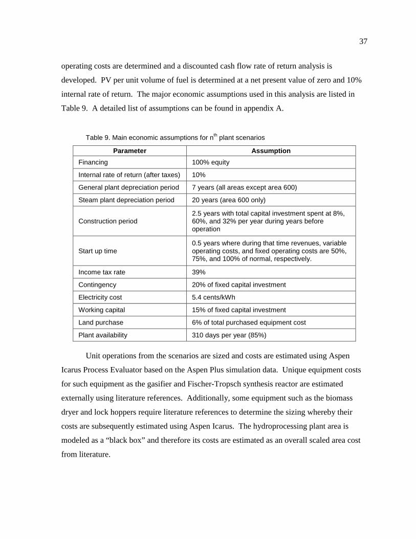
37

operating costs are determined and a discounted cash flow rate of return analysis is

developed. PV per unit volume of fuel is determined at a net present value of zero and 10%

internal rate of return. The major economic assumptions used in this analysis are listed in

Table 9. A detailed list of assumptions can be found in appendix A.

Table 9. Main economic assumptions for nth plant scenarios

Parameter Assumption

Financing 100% equity

Internal rate of return (after taxes) 10%

General plant depreciation period 7 years (all areas except area 600)

Steam plant depreciation period 20 years (area 600 only)

Construction period 2.5 years with total capital investment spent at 8%, 60%, and 32% per year during years before operation

Start up time 0.5 years where during that time revenues, variable operating costs, and fixed operating costs are 50%, 75%, and 100% of normal, respectively.

Income tax rate 39%

Contingency 20% of fixed capital investment

Electricity cost 5.4 cents/kWh

Working capital 15% of fixed capital investment

Land purchase 6% of total purchased equipment cost

Plant availability 310 days per year (85%)

Unit operations from the scenarios are sized and costs are estimated using Aspen

Icarus Process Evaluator based on the Aspen Plus simulation data. Unique equipment costs

for such equipment as the gasifier and Fischer-Tropsch synthesis reactor are estimated

externally using literature references. Additionally, some equipment such as the biomass

dryer and lock hoppers require literature references to determine the sizing whereby their

costs are subsequently estimated using Aspen Icarus. The hydroprocessing plant area is

modeled as a “black box” and therefore its costs are estimated as an overall scaled area cost

from literature.

38

The costs of each equipment or area are scaled based on a scaling stream and scaling

size factor (') according to equation 12 where the size factor is between 0.6-1.0 depending

on the equipment type.

�()*+,- � �()*. / ��*0�1� �23�+,-�*0�1� �23�.

#+ (eqn. 12)

All purchased equipment costs determined via Aspen Icarus contain an installation

factor that accounts for piping, electrical, and other costs required for installation. However,

this installation factor tends to be significantly lower than metrics suggested by Peters et

al.[51] Therefore, rather than using the software-derived installation factors, an overall

installation factor is applied to most equipment. A 3.02 overall installation factor is used as

suggested by Peters et al. for solid-liquid plants. Basically, the purchased equipment cost of

a piece of equipment is multiplied by the installation cost to determine its installed cost. For

the gasification unit, a 2.35 installation factor is used according to a National Energy

Technology Laboratory study by Reed et al.[52] It is assumed that all gas compressors

receive a 1.2 installation factor which is consistent with Aspen Icarus. The Chemical

Engineering Plant Cost Index is used to bring the cost to $2007 wherever a source for an

estimated cost is from a previous year [53]. For multiple unit operations that operate in

parallel or in trains, a train cost factor is applied. The reason for the factor, as reported by

Larson et al. [39], is because those units share some of piping, electrical, and other

installation costs. It is applied as shown in equation 13 where ' is the number of units in the

train and � is the train factor with value of 0.9.

�()*4567+ � �()*8+74 / '9 (eqn. 13)

Table 10 explains the methodology undertaken to estimate capital investment. After

total purchased equipment cost (TPEC) and total installed cost (TIC) are determined, indirect

costs are applied. Indirect costs (IC) include engineering and supervision, construction

expenses, and legal and contractor’s fees at 32%, 34%, and 23% of TPEC, respectively [51].

Project contingency is added as 20% of total direct and indirect cost (TDIC). TDIC is set as

the sum of TIC and total installed costs (TIC). With project contingency added the Fixed

39

Capital Investment is determined. Total Capital Investment (TCI) is determined by adding

working capital to Fixed Capital Investment and thereby represents the overall investment

required for each scenario.

Table 10. Methodology for capital cost estimation for nth plant scenarios

Parameter Method

Total Purchased Equipment Cost (TPEC) Aspen Icarus Process Evaluator®, references

Total Installed Cost (TIC) TPEC * Installation Factor

Indirect Cost (IC) 89% of TPECa

Total Direct and Indirect Costs (TDIC) TIC + IC

Contingency 20% of TDIC

Fixed Capital Investment (FCI) TDIC + Contingency

Working Capital (WC) 15% of FCI

Total Capital Investment FCI + WC

(a) indirect costs are broken down into engineering and supervision, construction expenses,

and legal and contractor’s fees at 32%, 34%, and 23%, respectively, for a total of 89% of

TPEC.

Raw material costs are inflated to 2007$ using the Industrial Inorganic Chemical

Index also used by Phillips et al. Annual variable operating costs are determine from material

stream flows. Variable operating costs and respective cost method is shown in Table 11.

Natural gas for use in the gas turbine to produce power during startup and backup periods is

assumed to be employed 5% of the annual operating time. Solids disposal costs are for the

handling and removal of ash in the LT scenario and slag in the HT scenario. Wastewater

disposal cost is applied to the sludge and black water produced during direct syngas quench.

Catalyst costs are not calculated on an annual basis since the catalysts for all reactors are

assumed to be replaced every 3 years. Instead they are accounted for in the discounted cash

flow analysis.

40

Table 11. Variable operating cost parameters adjusted to 2007$

Variable Operating Costs Cost information

Feedstock $75/dry short ton

LO-CAT Chemicals $176/metric ton of sulfur produced as reported in Peters et al. [40]

Amine make-up $1.09/lb as reported in Phillips et al. and set as 0.01% of the circulating rate [40]

Process Steam $8.20/ton (Peters et al.) [51]

Cooling water $0.31/ton (Peters et al.)

Hydroprocessing $4.00/barrel produced as reported by Robinson and Dolbear [54]

Natural gas (for backup) $6.40/thousand standard cubic feet as the average wellhead price for 2007 [55]

Ash/Char disposal $23.52/ton[40]

Wastewater disposal $3.30/hundred cubic feet [40]

Electricity $0.054/kWha

Sulfur $40.00/ton [40]

Fischer-Tropsch catalyst (cobalt)

$15/lb and 64lb/ft3 density; applied on first operation year and then every three yearsa

Water-gas-shift catalyst (copper-zinc)

$8/lb and 900kg/m3; applied on first operation year and then every three years. Sour shift and normal WGS are assumed to operate with same catalysta

Steam methane reforming catalyst (nickel-aluminum)

$15/lb and 70lb/ft3; applied on first operation year and then every three yearsa

Pressure swing adsorption $2/lba

(a) assumed

Fixed operating costs include employee salaries, overhead, and maintenance, and

insurance and taxes. Salaries are calculated similarly to Phillips et al. [40] where employees

include a plant manager, shift supervisors, lab technician, maintenance technician, shift

operators, yard workers, and office clerks. The labor index developed by the Bureau of

Labor Statistics [56] is used to adjust the labor cost to 2007$. Overhead is calculated as 60%

of total salaries; maintenance cost and taxes/insurance cost are both 2% of total installed

equipment cost as in accordance with Aden et al.[57]

For the DCFROR analysis, the capital investment is spent over a 2.5 year

construction period, with 8% in the first half year, followed by 60% and 32% for the next

two years. Working capital is applied in the year before operation and recovered at the end of

the plant life. A standard modified accelerated cost recovery system (MACRS) is used, with

41

the steam plant depreciating over 20 years and the rest of the plant over a 7 year period

consistent with IRS allowances. The project life is 20 years. Plant availability of 310 days

per year (85%) is assumed and affects raw materials purchase as well as fuel production.

The PV per gallon of gasoline equivalent is calculated for a set net present value of zero

including a 10% internal rate of return.

3.3.1 Methodology for Major Equipment Costs

The software used for determining equipment costs is not capable of estimating every

unit in this study. Some units such as the gasifiers and Fischer-Tropsch reactors are unique

pieces of equipment that are underestimated if estimated as a simple vertical pressure vessel.

Therefore, literature sources have been used to help estimate sizes and costs of many units.

The following section details a few of the more important units.

The biomass dryer costs are estimated by determining the drying contact area.

According to Couper [58], typical rotary dryers have a diameter of 6 feet and solids holdup

of 8%. Assuming a bulk density of 100 kg/m3 for ground stover and 1000 kg/m3 for moisture

in the stover, the resulting total surface area required for drying is 1880 m2. The surface area

provides enough information for estimating the costs since rotary dryer costs are estimated

based on surface area in Aspen Icarus. Details on dryer sizing can be found in section 5 of

appendix C.

The lock hopper system sizes are estimated by referring to a Department of Energy

report completed by Combustion Engineering, Inc. [59] where residence times and operating

pressures are given. The biomass receiving bin, lock hopper, and feed bin costs are then

estimated with Aspen Icarus. Details on lock hopper sizing can be found in section 5 of

appendix C.

The high temperature gasifier cost is estimated from Reed et al. [52] The total bare

erected cost (installed cost) of a train of 8 high temperature E-Gas™ gasifiers (2500 metric

ton per day coal) including syngas cooling costs is $638 million (2006$). It is assumed that

the syngas cooling accounts for 20% of that cost and therefore the estimated installed cost in

millions of 2006$ for a 2000 metric ton per day high temperature gasifier follows the formula

in equation 14 resulting in $57 million installed.

42

�()*!:;6<7=7,5 � �638 · 80%�8 · �2000@�

2500@�#..A

(eqn. 14)

A fluidized bed gasifier installed cost is described in Larson et al. [39] and is

calculated as shown in equation 15 where �()*._;6<7=7,5 is $6.41 million ($2003),

�*0�1� �23�. is 41.7 metric ton per hour, and ' is 0.7. The gasifier is evaluated at 300 short

tons per day because that appears to be the highest proven capacity for GTI gasifier.

Therefore, seven fluidized bed gasifiers are used in parallel. It is assumed that the gasifier

train follows the train cost formula (equation 13) resulting in $19 million installed.

�()*C:;6<7=7,5 � �()*._;6<7=7,5 / � �*0�1� �23��*0�1� �23�.

#+ (eqn. 15)

In a similar manner the FT reactor is estimated as described in Larson et al. [39]

where base installed cost is $10.5 million ($2003), base sizing value is 2.52 million standard

cubic feet per hour of synthesis gas flow, and sizing exponent of 0.72. A installation factor

of 3.6 is assumed for the FT reactor as found in Peters et al. [51] for liquid production plants.

This allows the purchased cost of the unit to be back calculated.

The acid gas removal (AGR) area cost is evaluated using information from Phillips et

al. [40] following equation 12 where the base stream size is 4000 short tons per day and base

cost is $5.45 million. The stream size is the mass flow of the synthesis gas entering the AGR

as the sum of fresh syngas from gas scrubbing and unconverted syngas from fuel synthesis

area.

Capital investment for the hydroprocessing area is found in Robinson et al.[54] That

study reports a volumetric unit cost of $4,000 per barrel per standard day. Assuming the

typical hydroprocessing refinery produces 25,000 barrels per day the base cost, C0, is $100

million. Assuming a scaling exponent of 0.65, the cost of area 500 is found using equation

12. The cost details of both gasifiers, AGR area, FT reactor, and hydroprocessing area can

be found in section 5 of appendix C.

43

3.3.2 Methodology for Sensitivity Analysis

Sensitivity parameters are chosen to reflect the change in PV. The parameters are

either economic or process parameters. The sensitivity bounds are chosen as what is

expected to be observed in the construction and operation of a biomass-to-liquids production

plant. The chosen favorable, baseline, and unfavorable sensitivity variables are shown in

Table 12.

Table 12. Sensitivity parameters for nth plant scenarios

Parameter Favorable Baseline Unfavorable

Availability (hours/year) 8000 7446 7000

Balance of Plant (% of TPEC)a 8 12 16

Catalyst cost (%)b 50 100 200

Catalyst lifetime (year) 5 3 1

CO conversion in FT reactor (%) 30 40 50

Compressor Install factor 1.0 1.2 3.0

Contingency (% of TDIC)c 10 20 30

Feedstock Cost ($/dry short ton) 50 75 100

Feedstock Moisture (%wet) 20 25 30

Price of Electricity (¢/kWh) 7.0 5.4 3.0

Total Capital Investment (% of baseline) 70 100 130

(a) TPEC=total purchased equipment cost (b) All catalyst costs are varied over this range (c) TDIC=total direct and indirect cost

3.3.3 Methodology for Pioneer Plant Analysis

Economic analysis is based on an nth plant design and before a project is undertaken

the pioneer (1st) plant cost is important to estimate. This method begun by the RAND

Corporation estimates pioneer plant costs and plant performance. Using this methodology,

two main areas of the nth plant economic analysis are adjusted: capital investment and plant

performance. Through a series of parameters, a cost inflation factor is generated to inflate

the capital investment. In addition, a plant performance factor is calculated which reduces

the fuel sales, feedstock purchase, and variable operating costs for first several years that the

plant is in operation. Each year the plant performance factor is increased until full

performance is attained. For the purpose of determining a range of pioneer plant costs

44

baseline, optimistic, and pessimistic values are chosen. The details of the RAND

methodology can be found in Merrow et al.[60] The following section explains the

reasoning behind the parameters chosen for the scenarios.

Cost growth and plant performance factors are calculated as shown in equations 16

and 17 in accordance with Merrow et al. [60] The

�()* D0(E*F � 1.1219 � 0.00297 / H���IJ � 0.02125/ K@HLMK�KI� � 0.01137 / ��@HNIOK�P � 0.00111/ K��NL�KQI�I�� � 0.06351/ HM�RI�� SITK�K�K��

(eqn. 16)

HU1'* H�0V. � 85.77 � 9.69 / �IJ��IH� � 0.33 / WXNIY� � 4.12/ JX��I � 17.91 / ��NKS�

(eqn. 17)

The factors are applied to the capital investment and plant performance as shown in

equations 18 and 19. Expenses and revenues affected by the plant performance factor are

fuel sales, feedstock purchase, co-product credits, and variable operating costs.

��K[7\+,,5 � ��K+4]�()* D0(E*F (eqn. 18)

The �()* D0(E*F factor causes the TCI of the pioneer plant to increase from nth plant.

�()*[7\+,,5�*� � �()*+4]�*� / �HU1'* H�0V. � 20 / �* � 1��100 (eqn. 19)

�()*+4]�*� is the nth plant expense or revenue at year *. The plant performance factor

is applied at year 1 and increases by 20% each year until 100% performance is reached. The

chosen parameters and calculated factors for baseline, optimistic, and pessimistic are shown

in Table 13. Details of variables found in equation 16 and 17 and the chosen values are

explained in section 5 of appendix B.

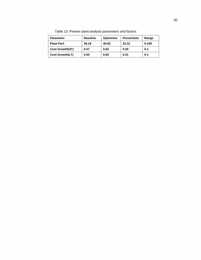
45

Table 13. Pioneer plant analysis parameters and factors

Parameter Baseline Optimistic Pessimistic Range

Plant Perf. 38.18 49.93 22.31 0-100

Cost Growth(HT) 0.47 0.63 0.30 0-1

Cost Growth(LT) 0.50 0.65 0.31 0-1

46

4. RESULTS AND DISCUSSION

4.1 Process Results

Along with lower fuel yield, the LT scenario consumes less power (Table 14). The

LT scenario and HT scenario total power usage is 15 and 22 MW, respectively. Major

contributions to this result are a lower grinder power due to less strict biomass size

requirement, lower pressurized oxygen consumption in gasifier, and generally lower

downstream mass flow rates throughout the plant for the LT scenario. A lower syngas yield

also means that there is less unconverted syngas and fuel gas from the hydroprocessing area

available for the gas turbine. Therefore, the LT scenario generates 31 MW compared to 36

MW as generated by the HT scenario. Due to unoptimized flow rates of the recycle streams,

the LT scenario actually generates a net 16 MW of power, which is more than the 14 MW

produced in the HT scenario. Reducing the net power generation is achievable by increasing

the recycle ratio and thereby increasing conversion, but a consequence is higher flow rates

and therefore larger and more expensive equipment. The focus of this study is to produce

liquid fuels. However, procedures to optimize recycle ratios, equipment sizes, and fuel

production rates are not within the scope of this study and are not undertaken.

Table 14. Power generation and usage

Power (MW) HT Scenario LT Scenario USAGE

Chopper 0.50 0.50

Grinder 2.96 1.10

Lock hopper system 0.18 0.18

Lean Amine Solution Pump 0.86 0.69

Syngas Booster Compressor 1.25 0.96

PSA Compressor 0.15 0.11

Recycle Compressor 0.39 0.29

Hydroprocessing Area 2.24 1.73

Oxygen compressor (ASU) 3.61 2.80

Air Compressor (ASU) 7.94 6.31 Sour Gas Shift Steam Compressor 1.59 0

CO2 Compressor 0.39 0.39 Total Usage 22.06 15.06 GENERATION

Gas Turbine 26.25 21.02

Steam Turbine 9.63 10.40

Total Generated 35.88 31.42 Net Export 13.82 16.36

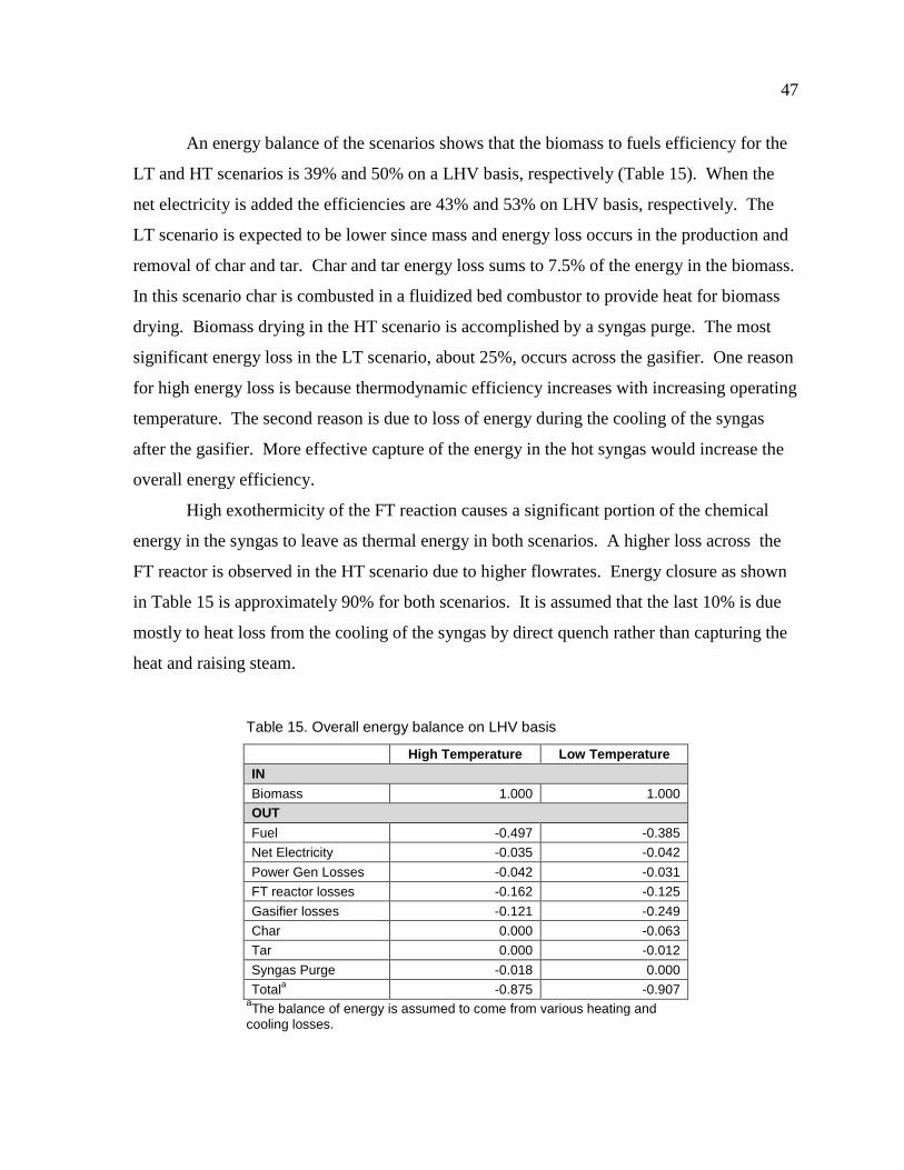
47

An energy balance of the scenarios shows that the biomass to fuels efficiency for the

LT and HT scenarios is 39% and 50% on a LHV basis, respectively (Table 15). When the

net electricity is added the efficiencies are 43% and 53% on LHV basis, respectively. The

LT scenario is expected to be lower since mass and energy loss occurs in the production and

removal of char and tar. Char and tar energy loss sums to 7.5% of the energy in the biomass.

In this scenario char is combusted in a fluidized bed combustor to provide heat for biomass

drying. Biomass drying in the HT scenario is accomplished by a syngas purge. The most

significant energy loss in the LT scenario, about 25%, occurs across the gasifier. One reason

for high energy loss is because thermodynamic efficiency increases with increasing operating

temperature. The second reason is due to loss of energy during the cooling of the syngas

after the gasifier. More effective capture of the energy in the hot syngas would increase the

overall energy efficiency.

High exothermicity of the FT reaction causes a significant portion of the chemical

energy in the syngas to leave as thermal energy in both scenarios. A higher loss across the

FT reactor is observed in the HT scenario due to higher flowrates. Energy closure as shown

in Table 15 is approximately 90% for both scenarios. It is assumed that the last 10% is due

mostly to heat loss from the cooling of the syngas by direct quench rather than capturing the

heat and raising steam.

Table 15. Overall energy balance on LHV basis

High Temperature Low Temperature IN

Biomass 1.000 1.000 OUT

Fuel -0.497 -0.385

Net Electricity -0.035 -0.042

Power Gen Losses -0.042 -0.031

FT reactor losses -0.162 -0.125

Gasifier losses -0.121 -0.249

Char 0.000 -0.063

Tar 0.000 -0.012

Syngas Purge -0.018 0.000

Totala -0.875 -0.907 aThe balance of energy is assumed to come from various heating and cooling losses.

48

A carbon balance analysis shows that 26 and 34 percent of the carbon in the biomass

is passed on to the fuels for the LT and HT scenarios, respectively (Table 16).

Approximately 99% of the carbon is accounted for. Major carbon losses include carbon

dioxide flue gases, LO-CAT venting and lock hopper venting. Char leaving the LT scenario

is accounted for in the A200 flue gas since the char is combusted for process heat. Also

since the LT scenario produces low molecular weight hydrocarbons in the gasification

process, a small fraction become dissolved in the liquid effluent of the wet scrubber. Carbon

dioxide also dissolves in wet scrubber effluent stream. Another carbon loss comes from the

hydrocarbons that dissolve in the acid gas removal area.

Table 16. Overall carbon balance

HT scenario LT scenario

kmol/hr % kmol/hr %

IN

Biomass 3280.60 1.000 3280.60 1.000

OUT

Fuel 1111.28 0.339 861.60 0.263

A300 CO2 Vent 1458.41 0.445 1293.87 0.394

A600 Flue Gas 334.13 0.102 301.92 0.092

A200 Flue Gas 39.35 0.012 226.77 0.069

Lock hopper Vent 159.14 0.049 161.89 0.049

Wet Scrubber Effluent 154.38 0.047 318.30 0.097

Tar 0.00 0.000 34.58 0.011

Dissolved Hydrocarbons 0.00 0.000 45.90 0.014

Total 3256.69 0.993 3244.83 0.989

Throughout the scenarios steam and cooling water are required as utilities. Since a

pinch analysis (a method to optimize heat exchange) is not undertaken for this study,

integration of the heat streams is not optimized. Therefore, it is assumed that the resulting

heating and cooling requirements within the model represent steam and cooling water

utilities whereby they are recycled at a ratio of 9:1. In other words, fresh steam and cooling

49

water utility input to the scenarios are assumed to be calculated at 10% of the required

circulating rate.

4.2 Cost Estimating Results

4.2.1 Capital and Operating Costs for nth Plant

The breakdown of costs by area and resulting total capital investment is shown in

Table 17. Total capital investment for the HT and LT scenarios are $606 million and $498

million, respectively. Major areas of investment are the gasification area in the HT scenario

and the fuel synthesis area in the LT scenario. Moreover, these two areas contain significant

differences in capital investment between the scenarios. The installed cost of the entrained

flow gasifier is significantly higher than the fluidized bed gasifiers even when seven are used

in parallel. Area 400 costs of the LT scenario are higher than the HT scenario due to steam

methane reformer and additional heat exchange equipment required for the high operational

temperature. A significant portion of the capital cost is due to gas compression such as the

air compressor in the air separation unit and syngas booster compressor. Due to high

purchase costs, compressors make up approximately 18% of the TPEC for each scenario.

Detailed accounting of equipment found in each process area can be found in section 2 and 3

of appendix B.

50

Table 17. Capital investment breakdown for nth plant scenarios

High Temperature Low Temperature

Area Installed Cost Installed Cost

($MM) % ($MM) %

A100: Preprocessing 22.7 7 22.7 9

A200: Gasification 67.8 22 28.2 11

A300: Syngas Cleaning 33.5 11 29.3 12

A400: Fuel Synthesis 49.4 16 58.7 23

A500: Hydroprocessing 33.0 11 29.5 12

A600: Power Generation 45.6 15 38.9 15

A700: Air Separation Unit 24.3 8 19.5 8

Balance of Plant 33.1 11 27.2 11

Total Installed Cost 309.4 253.9

Indirect Cost 129.7 107.2

Total Direct and Indirect Cost 439.1 361.1

Contingency 87.8 72.2

Fixed Capital Investment 526.9 433.3

Working Capital 79.0 65.0

Total Capital Investment 605.9 498.3

Annualized costs for operation of the plant are shown in Table 18. The percentage

displayed also represents percentage of PV. The largest annual incurred costs for both

scenarios are the average return on investment and feedstock purchase. Utilities such as

steam and cooling water are higher for the LT scenario due to heating and cooling of the

syngas before and after the SMR and steam input to the SMR. Waste disposal costs are equal

since equal amount of ash or slag are by-products of the plants. Annual hydroprocessing area

costs and income taxes are higher for HT scenario because of higher fuel production rate.

Fixed costs and capital depreciation are higher due to higher TCI.

Catalyst costs are not determined on an annual basis since they are assumed to be

replaced every three years. Table 19 contains catalyst replacement costs. The catalyst cost

the ZnO guard bed and PSA unit are equal across the scenarios because the volumes of the

units are assumed to be the same. FT catalyst for the HT scenario is significantly more

expensive because of a higher gas flow rate and hence more catalyst. Using a DCFROR

analysis, the PV at a net present value of zero for the LT and HT scenarios are $4.83 and

51

$4.27 per gallon of gasoline equivalent, respectively. Further detail of the yearly cash flow

of the life of the plant can be found in section 4 of appendix B.

Table 18. Annual operating cost breakdown for nth plant scenarios

High Temperature Low Temperature

Annual cost (2007$) % Annual cost (2007$) %

Average Return on Investment $58,200,000 32.7% $48,300,000 31.0%

Feedstock $51,300,000 28.9% $51,300,000 32.9%

Capital Depreciation $26,300,000 14.8% $21,700,000 13.9%

Average Income Tax $21,900,000 12.3% $18,000,000 11.6%

Fixed Costs $14,300,000 8.1% $12,400,000 8.0%

Hydroprocessing $4,400,000 2.5% $3,000,000 2.0%

Steam $2,700,000 1.5% $3,500,000 2.2%

Cooling Water $2,300,000 1.3% $3,500,000 1.6%

Waste Disposal $1,500,000 0.3% $1,500,000 0.3%

Other Raw Matl. Costs $1,400,000 0.8% $1,300,000 0.8%

Co-product credits -$5,600,000 -3.1% -$6,600,000 -4.2%

Table 19. Catalyst replacement costs for both scenarios (3 year replacement period)

Catalyst HT scenario LT scenario

Water-gas-shift (copper-zinc) $114,621 $104,732

Steam reforming (nickel-aluminum) N/A $103,412

ZnO guard bed $424,410 $424,410

PSA packing $497,135 $497,135 Fischer-Tropsch (cobalt) $7,686,720 $6,127,680

4.2.2 Sensitivity Results for nth Plant

The results of sensitivity analysis are summarized in Figures 13 and 14 for the HT

and LT scenarios, respectively. Total capital investment and feedstock purchase cost have

the highest effect on the PV at approximately ±$0.80 and ±$0.40 per GGE, respectively, for

both scenarios. Due to the high percentage of equipment cost for compressors, the

compressor installation factor has a very high effect on PV as well. When the compressor

installation factor is increased to 3.0, which is the usual installation factor for most of the

equipment, the PV increases by $0.71 and $0.78 per GGE for the LT and HT scenarios,

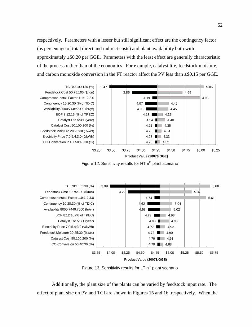
52

respectively. Parameters with a lesser but still significant effect are the contingency factor

(as percentage of total direct and indirect costs) and plant availability both with

approximately ±$0.20 per GGE. Parameters with the least effect are generally characteristic

of the process rather than of the economics. For example, catalyst life, feedstock moisture,

and carbon monoxide conversion in the FT reactor affect the PV less than ±$0.15 per GGE.

Figure 12. Sensitivity results for HT nth plant scenario

Figure 13. Sensitivity results for LT nth plant scenario

Additionally, the plant size of the plants can be varied by feedstock input rate. The

effect of plant size on PV and TCI are shown in Figures 15 and 16, respectively. When the

4.23

4.23

4.23

4.23

4.24

4.18

4.08

4.07

4.19

3.85

3.47

4.32

4.33

4.34

4.35

4.40

4.36

4.45

4.46

4.98

4.69

5.05

$3.25 $3.50 $3.75 $4.00 $4.25 $4.50 $4.75 $5.00 $5.25

CO Conversion in FT 50:40:30 (%)

Electricity Price 7.0:5.4:3.0 (¢/kWh)

Feedstock Moisture 20:25:30 (%wet)

Catalyst Cost 50:100:200 (%)

Catalyst Life 5:3:1 (year)

BOP 8:12:16 (% of TPEC)

Availability 8000:7446:7000 (hr/yr)

Contingency 10:20:30 (% of TDIC)

Compressor Install Factor 1.1:1.2:3.0

Feedstock Cost 50:75:100 ($/ton)

TCI 70:100:130 (%)

Product Value (2007$/GGE)

4.79

4.79

4.78

4.77

4.80

4.73

4.63

4.62

4.74

4.29

3.99

4.88

4.91

4.90

4.92

4.98

4.93

5.02

5.04

5.61

5.37

5.68

$3.75 $4.00 $4.25 $4.50 $4.75 $5.00 $5.25 $5.50 $5.75

CO Conversion 50:40:30 (%)

Catalyst Cost 50:100:200 (%)

Feedstock Moisture 20:25:30 (%wet)

Electricity Price 7.0:5.4:3.0 (¢/kWh)

Catalyst Life 5:3:1 (year)

BOP 8:12:16 (% of TPEC)

Availability 8000:7446:7000 (hr/yr)

Contingency 10:20:30 (% of TDIC)

Compressor Install Factor 1.0:1.2:3.0

Feedstock Cost 50:75:100 ($/ton)

TCI 70:100:130 (%)

Product Value (2007$/GGE)

53

plant size is reduced to 500 MT/day the two scenarios approach equal PV. Also, as the plant

size is reduced from the baseline, the difference in capital investment decreases. As the plant

size increases past the baseline the slope of PV levels out suggesting that the benefits of

lower PV may not be worth the significant increase in capital cost (Figure 14).

Figure 14. The effect of plant size on product value (per gallon of gasoline equivalent) for nth plant scenarios

Figure 15. The effect of plant size on total capital investment for nth plant scenarios

0.00

1.00

2.00

3.00

4.00

5.00

6.00

7.00

0 500 1000 1500 2000 2500 3000 3500 4000 4500 5000 5500

Pro

du

ct v

alu

e (

$/G

GE

)

Plant Size (metric ton/day)

HT Scenario

LT Scenario

0

200

400

600

800

1000

1200

0 500 1000 1500 2000 2500 3000 3500 4000 4500 5000 5500

To

tal c

apit

al in

vest

men

t ($

MM

)

Plant Size (metric ton/day)

HT Scenario

LT Scenario

base

base

54

4.2.3 Pioneer Plant Analysis Results

The total capital investment for a base case pioneer plant is expected to double from

the nth plant scenarios as detailed in Table 20. PV for a base case pioneer plant of the LT and

HT scenario are estimated to increase to $7.20 and 7.70 per GGE, respectively. Table 20

presents further shows estimates of the optimistic and pessimistic cases. An important

observation is that the PV for the LT scenario is actually lower than the HT scenario. The

reason behind this inverted result is because of the higher capital cost inflation (cost growth

factor) in the HT scenario due to higher gasification area capital costs.

Table 20. Pioneer Plant Analysis Results

Analysis HT Scenario LT Scenario

TCI ($MM) PV ($/GGE) TCI ($MM) PV ($/GGE)

nth Plant 606 4.27 498 4.83

1st Plant Base 1290 7.70 997 7.20

1st Plant Optimistic 960 6.00 768 6.00

1st Plant Pessimistic 2050 11.80 1602 10.80

4.3 Comparison with Previous Techno-economic Studies

Two previous BTL studies that specifically use biomass feedstock, low temperature

gasification, and Fischer-Tropsch synthesis technology are Tijmensen et al [41]. and Larson

et al. [39] In order to compare, major economic and process parameters from the present nth

plant LT scenario are adjusted to reflect similar values to the previous studies. First, the

plant size of the present study is adjusted to increase equipment costs and raw materials

purchases. As a result the annual biomass input and TCI is affected. Second, availability in

hours per year, rate of return, cost year, and feedstock cost is adjusted. The combined effect

of all adjusted parameters causes the present study’s product value to reflect the comparison

study.

A comparison to the IGT-R scenario (which employs a low temperature, IGT gasifier

and a steam methane reformer) in Tijmensen et al. shows that fuel product value is higher in

the present study as summarized in Table 21. Of all the scenarios developed by Tijmensen et

al, the IGT-R scenario is most similar to the present study because of the reformer. The IGT-

55

R scenario has a TCI of $387 million, feedstock cost of $33 per short ton, and a product

value of $1.90/GGE. An important characteristic of the Tijmensen et al. study is that it does

not include a hydroprocessing area. Therefore, it is expected that the TCI would be higher

for the present study since hydroprocessing is included. However, that is not the case since

the TCI of the present study using Tijmensen et al. parameters is $339 million which is lower

than the reported $387 million. Another important observation is that the annual fuel

production for the present study with adjusted parameters is 30.2 million gallons per year

compared to 39.8 million gallons per year of FT products reported by Tijmensen et al. One

reason for lower annual fuel production in the present study is because of a loss during

hydroprocessing. Therefore, due to lower annual fuel production and hence lower fuel

revenue, the present study has higher product value compared to Tijmensen et al.

Table 21. Comparison of nth plant LT scenario to Tijmensen et al. study [41]

Parameter Tijmensen et al.

study (IGT-R scenario)

Present study nth plant LT scenario

Present study w/ Tijmensen et al.

parameters

Plant Size (dry tons / day) 1920 2205 1920

Annual Biomass Input (tons) 640000 684100 640000

Total Capital Investment ($MM) 387 498 339

Availability (hour/year) 8000 7446 8000

Rate of Return (%) 10 10 10

Cost Year 2000 2007 2000

Feedstock Cost ($/short ton) 33.00 75.00 33.00

Efficiency (%, LHV, incl. elec.) 50.1 42.7 42.7

Fuel Yield (MMGGE/yr) 39.8 32.3 30.2

Product Value ($/GJ) 16.50 39.80 25.17

Product Value ($/GGE) 2.00 4.83 3.05

A comparison to the FT-OT-VENT scenario (which is low temperature gasification

with carbon dioxide vent and once through FT synthesis) reported by Larson et al. is

summarized in Table 22. In a similar fashion to the previous comparison the parameters

were adjusted to approximate the comparison study. Some important observations are made

from this comparison. First, the TCI of the present study with adjusted parameters is

significantly higher. Second, the net electricity is significantly lower for the present study.

56

Third, the PV is significantly higher for the present study. Essentially, the Larson et al. study

generates more revenue from selling electricity and recovers the capital investment in less

time. In addition, annual operating costs for the Larson et al. study are lower than the present

study. Therefore, the present study has a higher fuel product value when compared on a

similar basis to Larson et al.

Table 22. Comparison of nth plant LT scenario to Larson et al. study [39]

Parameter Larson et al.

study (FT-OT-VENT scenario)

Present study nth plant LT scenario

Present study with Larson et al. parameters

Plant Size (dry tons / day) 5000 2205 5001

Annual Biomass Input (tons) 1458000 684000 1459000

Total Capital Investment ($MM) 541 498 678

Availability (hour/year) 7000 7446 7000

Debt/Equity (% Equity) 60 100 60

Rate of Return (%) 12 10 12

Cost Year 2003 2007 2003

Electricity Price (cents/kWh) 4.0 5.4 4.0

Net Electricity (MW) 207 16.3 37.1

Feedstock Cost ($/short ton) 46.00 75.00 46.00

Plant Yield (MMGGE/yr) 63.3 32.3 68.9

Product Value ($/GJ) 15.25 39.80 26.80

Product Value ($/GGE) 1.85 4.83 3.25

4.4 Summary of nth plant scenarios

The HT scenario requires more power and capital investment, yields more fuel per

ton of feedstock, and subsequently produces more fuel per year compared to the LT scenario.

The total capital investment for the LT and HT scenarios are $498 million and $606 million,

respectively. Despite higher capital investment for the HT scenario, the product value (PV)

is lower. PV for the LT and HT scenarios are $4.83 and $4.27 per gallon of gasoline

equivalent, respectively. The main reason for a lower PV is because of increased fuel

revenue. The main nth plant scenario results are shown in Table 23. A detailed summary of

costs can be found in section 1 of appendix B.

57

Table 23. Main scenario nth plant results (TCI=total capital investment; TPEC=total purchased equipment cost; MM=million; GGE=gallon of gasoline equivalent)

Scenario TCI ($MM)

TPEC ($MM)

Fuel Yield (GGE/metric ton)

Annual Fuel Output

(MMGGE/yr)

Net Electricity

Export (MW)

PV ($/GGE)

High Temperature 605.9 145.7 61.0 41.7 13.8 4.27

Low Temperature 498.3 120.4 47.2 32.3 16.4 4.83

58

5. CONCLUSIONS

This analysis compares capital and operating cost for two biomass-to-liquids

scenarios: high temperature (HT) gasification and low temperature (LT) gasification. The

selection of these scenarios allow for direct comparison between two modes of gasification:

slagging and non-slagging. The slagging, entrained flow gasifier employed for the HT

scenario results in higher plant costs (about 20%) than the LT scenario, which employs a

fluidized bed gasifier. The higher carbon conversions for the HT gasifier, on the other hand,

results in a lower PV compared to the LT scenario. Biomass-to-liquids is expected to

produce fuels costing in the range of $4-$5 per gallon gasoline equivalent using present

gasification and Fischer-Tropsch synthesis technology. The factors chiefly responsible for

this relatively high PV is feedstock costs and investment return on the capital to build a $500

million to $650 million plant to process 2000 metric tons per day. A pioneer plant analysis

estimates that the total capital investment for a pioneer plant would double and PV would

increase by approximately 60% from the nth plant scale. This uncertainty suggests that

economics are yet to be a major challenge for biomass-to-liquids production plants.

The most sensitive effects on PV are total capital cost, feedstock purchase cost, and

compressor installation factor affecting the PV between ±$0.40-0.80 per gallon. Less

expensive biomass feedstock that is lower in ash content than used in the present study will

have higher fuel yield and have the potential to significantly decrease PV. Gas compression

is a major portion of capital investment and sensitivity analysis shows installation costs of

compressors have a high effect on PV. Factors with little effect on the PV are mostly related

to the process such as carbon monoxide conversion in the FT reactor, feedstock inlet

moisture, and catalyst lifetime.

Due to time and resource constraints, the technoeconomic study presented includes a

few shortcomings. The process configuration is not fully optimized by means of heat

integration. While some recycle streams are included, a complete heat exchange network for

heat recovery is not conceptualized. In addition, some areas such as FT product separation

and hydroprocessing are not modeled rigorously and can be improved with detailed mass and

energy flows.

59

REFERENCES

1. Frey HC. Akunuri N. Probabilistic Modeling and Evaluation of the Performance,

Emissions, and Cost of Texaco Gasifier-based Integrated Gasification Combined Cycle Systems using ASPEN. North Carolina State University: Raleigh, January, 2001.

2. Bain RL. Material and Energy Balances for Methanol from Biomass Using Biomass Gasifiers. NREL/TP-510-17098; National Renewable Energy Laboratory: January, 1992.

3. "economy." In The American Heritage® Dictionary of the English Language, Fourth ed.; Houghton Mifflin Company 2004.

4. Brown RC, Biorenewable resources : engineering new products from agriculture. Iowa State Press: Ames, Iowa, 2003.

5. de Swaan Arons J, van der Kooi H. Sankaranarayanan K, Biomass Production and Conversion. In Efficiency and Sustainability in the Energy and Chemical Industries, Marcel Dekker, Inc.: New York, 2004.

6. Cushman JH, et al. Roadmap for Agriculture Biomass Feedstock Supply in the United States. DOE/NE-ID-11129; Department of Energy: 2003.

7. Greene N, et al. Growing energy: How biofuels can help end America's oil dependence. National Resources Defense Council: December, 2004.

8. Knoef H, Practical Aspects of Biomass Gasification. In Handbook Biomass Gasification, Knoef, H., Ed. BTG Biomass Technology Group: Enschede, Netherlands, 2005.

9. Knoef H, History of Biomass Gasification. In Handbook Biomass Gasification, Knoef, H., Ed. BTG biomass technology group: Enschede, Netherlands, 2005.

10. Probstein RF. Hicks RE, Synthetic Fuels. Dover Publications: Mineola, NY, 2006.

11. Prins MJ. Thermodynamic analysis of biomass gasification and torrefaction. Technische Universiteit Eindhoven, Eindhoven, 2005.

12. McKendry P. Energy production from biomass (part 3): gasification technologies. Bioresource Technology 2002, 83, (1), 55-63.

13. Warnecke R. Gasification of biomass: comparison of fixed bed and fluidized bed gasifier. Biomass and Bioenergy 2000, 18, (6), 489-497.

60

14. Ciferno JP. Marano JJ. Benchmarking Biomass Gasification Technologies for Fuels, Chemicals, and Hydrogen Production. National Energy Technology Laboratory: June, 2002.

15. Williams RH, et al. Methanol and Hydrogen from Biomass for Transportation. Energy for Sustainable Development 1995, 1, (5), 18-34.

16. van der Drift H, et al. Entrained Flow Gasification of Biomass: Ash Behavior, Feeding Issues, and System Analyses. ECN-C--04-039; Energy Research Center of the Netherlands: April, 2004.

17. Henrich E. Weirich F, Pressurised Entrained Flow Gasifiers for Biomass. In Annual International Conference on Thermal Treatment Technologies, New Orleans, Louisiana, 2002.

18. Henrich E, et al., Clean Syngas from Bio-oil/Char Slurries. In Science in Thermal and Chemical Biomass Conversion, Bridgwater, A. V.; Boocock, D. G. B., Eds. CPL Press: Newbury, UK, 2006; Vol. 2, pp 1565-1579.

19. Naimi LJ, et al., Cost and Performance of Woody Biomass Size Reduction for Energy Production. In CSBE/SCGAB 2006 Annual Conference, American Society of Agricultural and Biological Engineers: Edmonton, Alberta, 2006.

20. Amos WA. Report on Biomass Drying Technology. NREL/TP-570-25885; November, 1998.

21. Zwart RWR, Boerrigter H. vanderDrift A. The Impact of Biomass Pretreatment on the Feasibility of Overseas Biomass Conversion to Fischer-Tropsch Products. Energy & Fuels 2006, 20, (5), 2192-2197.

22. Craig KR. Mann MK. Cost and performance analysis of biomass-based integrated gasification combined-cycle (BIGCC) power systems. NREL/TP--430-21657; 1996.

23. Stevens DJ. Hot Gas Conditioning: Recent Progress with Larger-scale Biomass Gasification Systems. NREL/SR-510-29952; National Renewable Energy Laboratory: Golden, CO, August, 2001.

24. Milne TA, Evans RJ. Abatzoglou N. Biomass Gasifier "Tars": Their Nature, Formation, and Conversion. NREL/TP-570-25357; National Renewable Energy Laboratory: Golden, CO, November, 1998.

25. Stevens DJ. Review and Analysis of the 1980-1989 Biomass Thermochemical Conversion Program. NREL/TP-421-7501; National Renewable Energy Laboratory: September, 1994.

61

26. Nexant Inc. Equipment Design and Cost Estimation for Small Modular Biomass Systems, Synthesis Gas Cleanup, and Oxygen Separation Equipment. NREL/SR-510-39945; National Renewable Energy Laboratory: May, 2006.

27. Wender I. Reactions of synthesis gas. Fuel Processing Technology 1996, 48, (3), 189-297.

28. Consonni S. Larson ED. Biomass-Gasifier/Aeroderivative Gas Turbine Combined Cycles: Part A - Technologies and Performance Modeling. Journal of Engineering of Gas Turbines and Power 1996, 118, (3), 507-515.

29. Bridgwater AV, Toft AJ. Brammer JG. A techno-economic comparison of power production by biomass fast pyrolysis with gasification and combustion. Renewable & Sustainable Energy Reviews 2002, 6, (3), 181-246.

30. Spath PL. Dayton DC. Preliminary Screening -- Technical and Economic Assessment of Synthesis Gas to Fuels and Chemicals with Emphasis on the Potential for Biomass-Derived Syngas. NREL/TP-510-34929; December, 2003.

31. Huber GW, Iborra S. Corma A. Synthesis of transportation fuels from biomass: Chemistry, catalysts, and engineering. Chemical Reviews 2006, 106, (9), 4044-4098.

32. Cocco D, Pettinau A. Cau G. Energy and economic assessment of IGCC power plants integrated with DME synthesis process. Proceedings of the Institution of Mechanical Engineers - Part A - Power & Energy 2006, 220, (2), 95-102.

33. Dry ME. The Fischer-Tropsch process: 1950-2000. Catalysis Today 2002, 71, (3-4).

34. Espinoza R, et al. Low temperature Fischer-Tropsch synthesis from a Sasol perspective. Applied Catalysis A: General 1999, 186, (1), 13-26.

35. Dry ME. Practical and theoretical aspects of the catalytic Fischer-Tropsch process. Applied Catalysis A: General 1996, 138, (2), 319-344.

36. Bridgwater AV. The technical and economic feasibility of biomass gasification for power generation. Fuel 1995, 74, (5), 631-653.

37. Larson ED, Jin H. Celik FE. Gasification-based Fuels and Electricity Production from Biomass, without and with Carbon Capture and Storage. Princeton University: Princeton, NJ, October, 2005.

38. Hamelinck CN, et al. Production of FT transportation fuels from biomass; technical options, process analysis and optimisation, and development potential. Energy 2004, 29, (11), 1743-1771.

62

39. Larson ED, Jin H. Celik FE. Large-scale gasification-based coproduction of fuels and electricity from switchgrass. Biofuels, Bioproducts, and Biorefining 2009, 3, (2), 174-194.

40. Phillips S, et al. Thermochemical Ethanol via Indirect Gasification and Mixed Alcohol Synthesis of Lignocellulosic Biomass. NREL/TP-510-41168; National Renewable Energy Laboratory: April, 2007.

41. Tijmensen MJA, et al. Exploration of the possibilities for production of Fischer Tropsch liquids and power via biomass gasification. Biomass and Bioenergy 2002, 23, (2), 129-152.

42. Lau FS, et al. Techno-Economic Analysis of Hydrogen Production by Gasification of Biomass. DE-FC36-01GO11089; Gas Technology Institute: December, 2002.

43. Mani S, Tabil LG. Sokhansanj S. Grinding performance and physical properties of wheat and barley straws, corn stover and switchgrass. Biomass and Bioenergy 2004, 27, (4), 339-352.

44. Higman C. van der Burgt MJ, Gasification. Elsevier/Gulf Professional Publishing: Boston, 2003.

45. Engineering Data Book. 12th, FPS. ed.; Gas Processors Suppliers Association: Tulsa, Oklahoma, 2004.

46. Merichem Company, LO-CAT H2S Removal. http://www.gtp-merichem.com/products/lo-cat/process.php (June 20, 2008)

47. Kohl AL. Nelson RB, Gas Purification. 5th ed.; Gulf Professional Publishing: Houston, 1997.

48. Imperial Chemical Industries, ltd., Agricultural Division, Catalyst handbook: with special reference to unit processes in ammonia and hydrogen manufacture. Wolfe: London, 1970.

49. Song H, et al. Operating strategies for Fischer-Tropsch reactors: A model-directed study. Korean Journal of Chemical Engineering 2004, 21, (2), 308-317.

50. Shah PP, et al. Fischer-Tropsch Wax Characterization and Upgrading. DOE/PC/80017-T1; UOP, Inc.: Des Plaines, IL, June 6, 1998.

51. Peters MS, Timmerhaus KD. West RE, Plant design and economics for chemical engineers. McGraw-Hill: New York, 2003.

52. Reed ME, et al. Baseline Technical and Economic Assessment of a Commercial Scale Fischer-Tropsch Liquids Facility. DOE/NETL-2007/1260; National Energy Technology Laboratory: 2007.

63

53. Chemical Engineering Plant Cost Index. In Chemical Engineering: 2008.

54. Robinson PR. Dolbear GE, Commercial Hydrotreating and Hydrocracking. In Hydroprocessing of Heavy Oils and Residua, Ancheyta, J.; Speight, J. G., Eds. CRC Press: Boca Raton, FL, 2007.

55. Energy Information Administration, U.S. Natural Gas Wellhead Price. http://tonto.eia.doe.gov/dnav/ng/hist/n9190us3m.htm (March 1 2009)

56. United States Bureau of Labor Statistics. Labor Index. 2008.

57. Aden A, et al. Lignocellulosic Biomass to Ethanol Process Design and Economics Utilizing Co-current Dilute Acid Prehydrolysis and Enzymatic Hydrolysis for Corn Stover. National Renewable Energy Laboratory: Golden, CO, June, 2002.

58. Couper JR, Process engineering economics. Marcel Dekker: New York, 2003.

59. CE IGCC Repowering Project Bins and Lockhoppers: Topical Report. Under contract DE-FC21-90MC26308; Combustion Engineering, Inc.: 1993.

60. Merrow EW, Phillips KE. Myers CW. Understanding Cost Growth and Performance Shortfalls in Pioneer Process Plants. Contract no. DE-AC01-79PE70078; Rand Corporation: 1981.

64

APPENDIX A. ASSUMPTIONS

A.1 Technoeconomic Model Assumptions

A.1.1 Financial Assumptions

• Capital Investment o Equity: 100% o Working Capital (% of FCI): 15%

• Depreciation Model o Zero Salvage Value for both general plant and steam/ power plant o Type of Depreciation: Double-Declining-Balance Depreciation Method (DDB) as per

IRS Modified Accelerated Cost Recovery System (MARCS) guidelines � Depreciation Period (Years):

• General Plant: 7 • Steam/Power System: 20

• Construction & Start-up: o Construction Period (Years): 2.5

� % Spent in Year “-3”: 8% � % Spent in Year “-2”: 60% � % Spent in Year “-1”: 32%

o Start-up Time (Years): 0.5 � Revenues (% of Normal): 50% � Variable Costs (% of Normal): 75% � Fixed Cost (% of Normal): 100%

• Other o Internal Rate of Return: 10% o Income Tax Rate: 39% o Operating Hours per Year: 8,406

A.1.2 Capital Costs

• Cost Year for Analysis: 2007; cost escalation is applied using the Chemical Engineering Plant Cost Index

• The plant is designed based on the State of the Technology, at the nth plant level of experience

• Most equipment installation factors are applied using Peters et al. for solid-fluid plants (i.e. 3.02 installation factor);

• Materials of construction are carbon steel, stainless steel, alloys and refractory where necessary

• Sensitivity parameter involving changes in equipment size or capacity are use scaling exponents available in literature.

A.1.3 Operating Costs

• Working capital is assumed to be 15% of the total capital investment • Annual maintenance materials are 2% of the total installed equipment cost • Boiler feedwater and wastewater treatment costs are derived from prior NREL work.

65

• Fresh cooling water and steam costs are calculated at 10% of the required circulation rate meaning a 9:1 ratio of water recycling.

• Employee salary estimation is same as that chosen by Phillips, et al. • Employee salaries are indexed to the year of 2007 following the data of the Bureau of Labor

Statistics

A.1.4 Feedstock, Products and By-Products

• Feedstock is corn stover (comprising stalks, leaves, cobs and husks) o Moisture content in the feedstock is 25%

• Feed rate is 2000 dry metric ton per day o The feedstock delivery logistics are not considered o The feedstock is delivered to the feed handling area of the plant

• Feed cost is assumed to be $75/dry short ton at the gate • Gasoline and diesel products are sold for over the fence • Gasoline energy content is 115000 BTU/gallon • Fly ash and slag incur a solids waste disposal cost • Solid sulfur and electricity are sold as by-product

A.1.5 Process Assumptions

For both scenarios, most of the process was modeled with the aid of Aspen Plus™ software. The process was divided by logical process areas which are named below: Area 100 - Preprocessing

• Biomass is dried down to 10% o Steam raised from hot flue gas is used to dry the feedstock o Steam to moisture removal ratio is set at 9:1 in accordance with Amos. o Heat is provided by combusting char and unreacted syngas

• Grinder reduces biomass to 6-mm or less o The energy required for grinding is calculated separately using literature correlations

by Mani et al. Area 200 - Gasification

• Scenario 1: Entrained flow gasifier is modeled using thermodynamic equilibrium • Scenario 2: Fluidized bed gasifier is modeled using a mass balance calculation • 95% purity oxygen produced from Air Separation Unit provides oxidizer • Carbon dioxide is used as solids pressurization gas • All char produced in LT scenario is combusted for process heat

Area 300 - Syngas Cleaning

• Particulates, tar and partial ammonia removal via wet scrubbing o Scrubbing water is recycled at 90% rate o Particulate handling (not modeled)

� High temperature gasifier: particulate decant slurry is sent back into slagging gasifier

� Low temperature gasifier: particulate decant slurry is piled and landfilled; excess water is sent to aerobic water treatment (not modeled)

o Makeup water compensates for water lost via particulate slurry

66

� Process water condensate is used as makeup water • Sour water-gas-shift occurs at equilibrium and is modeled as such. • Carbon dioxide, hydrogen sulfide and excess ammonia removal via amine scrubbing acid gas

removal (AGR) at pressure: o 99% of sulfur is removed and 90% of carbon dioxide o Monoethanolamine (MEA) is the scrubbing solvent o Carbon dioxide is vented following LO-CAT™ removal of H2S.

• Hydrogen Sulfide is converted to solid sulfur via LO-CAT™ oxidation (99% conversion) • Ammonia can be disposed of by decomposition (not modeled) in

o Gasifier burner (slagging gasifier) o Char and syngas combustor (fluidized bed gasifier)

• Zinc oxide and activated carbon guard bed polishing assumed (not modeled in detail) Area 400 - Fuel Synthesis

• Water-gas-shift occurs at equilibrium and is modeled as such. • Pressure swing adsorption (PSA) is employed to remove excess H2 at an efficiency of 85%

and 99% purity. o The PSA system employs two trains with 6 reactors each to account for all stages of

pressurization, depressurization, purging etc.; o PSA adsorbers are filled 2/3 with activated carbon and 1/3 with molecular sieve

• Syngas is catalytically converted to fuels by one step Fischer-Tropsch synthesis followed by wax hydrocracking and fuel separation

o FT synthesis employs cobalt catalyst o 40% syngas conversion to fuels o Part of the unconverted syngas is recycled

� A fraction of the recycle is sent to the AGR to prevent CO2 buildup. � The overall recycle ratio is about 1.9

• A syngas purge is used as fuel in the combustor side of the biomass dryer (only in HT scenario)

• Excess syngas is sent to a gas turbine for power production Area 500, 600, 700

• Hydroprocessing and product distillation costs are estimated as a “black box” based on literature capital cost and operating cost information from Robinson et al.

o Literature yield data is used for estimating the relative yields of gasoline and diesel

A.1.6 Miscellaneous

• Combustion occurs with 120% excess oxygen

67

APPENDIX B. DETAILED COSTS

B.1 Cost Summary

B.1.1 High Temperature Scenario Summary

Figure 16. Economic Analysis Summary for HT Scenario

Product Value ($/ gal) $4.26Total Product ion at Operat ing Capacity (MM gal / year) 41.7

Product Yield (gal / Dry US Ton Feedstock) 61.0Delivered Feedstock Cost $/ Dry US Ton $75

Internal Rate of Return (After-Tax) 10%Equity Percent of Total Investment 100%

Capital Costs Operat ing Costs (cents/ gal product ) Area 100: Pret reatment $22,700,000 7% Feedstock 123.0 28.9% Area 200: Gasificat ion $67,800,000 22% Steam 6.4 1.5% Area 300: Syngas Cleaning $33,500,000 11% Cooling Water 5.5 1.3% Area 400: Fuel Synthesis $49,400,000 16% Other Raw Materials 3.4 0.8% Area 500: Hydrocracking/ Hydrot reat ing $33,000,000 11% Waste Disposal 1.3 0.3% Area 600: Power Generat ion $45,600,000 15% Hydroprocessing 10.6 2.5% Area 700: Air Separat ion $24,300,000 8% Fixed Costs 34.4 8.1% Balance of Plant $33,100,000 11% Co-product credits -13.3 -3.1%

Capital Depreciat ion 63.0 14.8%Total Installed Equipment Cost $309,400,000 Average Income Tax 52.4 12.3%

Average Return on Investment 139.5 32.7%Indirect Costs 129,700,000 (% of TPI) 21.4% Operat ing Costs ($/ yr) Project Cont ingency 79,000,000 Feedstock $51,300,000

Steam $2,700,000Total Project Investment (TPI) $605,900,000 Cooling Water $2,300,000

Other Raw Mat l. Costs $1,400,000Installed Equipment Cost per Annual Gallon $7.42 Waste Disposal $1,500,000Total Project Investment per Annual Gallon $14.52 Hydroprocessing $4,400,000

Fixed Costs $14,300,000Loan Rate N/ A Co-product credits -$5,600,000Term (years) N/ A Capital Depreciat ion $26,300,000Capital Charge Factor 0.176 Average Income Tax $21,900,000

Average Return on Investment $58,200,000Gasifier Efficiency - HHV % 82.1Gasifier Efficiency - LHV % 87.9 Total Plant Elect ricity Usage (KW) 22,065Overall Plant Efficiency (incl. elect ricity) - HHV % 52.7 Elect ricity Produced Onsite (KW) 35,880Overall Plant Efficiency - LHV % 53.0 Elect ricity Purchased from Grid (KW) 0

Elect ricity Sold to Grid (KW) 13,815Availability (%) 85.0%Plant Hours per year 7446 Plant Electricity Use (KWh/ gal product ) 6.1

HT Biomass-to-Liquids Scenario Summary2,000 Dry Metric Tonnes Biomass per Day

All Currency in 2007$ and Volume in Gallons Gasoline Equivalent (GGE)High Temperature Entrained Flow Gasifier, Sulfur Removal, Fischer-Tropsch Synthesis, Hydroprocessing, Combined Cycle Power

68

B.1.2 Low Temperature Scenario Summary

Figure 17. Economic analysis summary for LT scenario

Product Value ($/ gal) $4.83Total Product ion at Operat ing Capacit y (MM gal / year) 32.3

Product Yield (gal / Dry US Ton Feedstock) 47.2Delivered Feedstock Cost $/ Dry US Ton $75

Internal Rate of Return (After-Tax) 10%Equity Percent of Total Investment 100%

Capital Costs Operat ing Costs (cents/ gal product) Area 100: Pret reatment $22,700,000 9% Feedstock 158.9 32.9% Area 200: Gasificat ion $28,200,000 11% Steam 10.9 2.2% Area 300: Syngas Cleaning $29,300,000 12% Cooling Water 7.8 1.6% Area 400: Fuel Synthesis $58,700,000 23% Other Raw Materials 4.1 0.8% Area 500: Hydrocracking/ Hydrotreat ing $29,500,000 12% Waste Disposal 1.5 0.3% Area 600: Power Generat ion $38,900,000 15% Hydroprocessing 9.4 2.0% Area 700: Air Separat ion $19,500,000 8% Fixed Costs 38.4 8.0% Balance of Plant $27,200,000 11% Co-product credits -20.4 -4.2%

Capital Depreciat ion 67.2 13.9%Total Installed Equipment Cost $253,900,000 Average Income Tax 55.9 11.6%

Average Return on Investment 149.5 31.0%Indirect Costs 107,200,000 (% of TPI) 21.5% Operat ing Costs ($/ yr) Project Cont ingency 65,000,000 Feedstock $51,300,000

Steam $3,500,000Total Project Investment (TPI) $498,300,000 Cooling Water $3,500,000

Other Raw Mat l. Costs $1,300,000Installed Equipment Cost per Annual Gallon $7.86 Waste Disposal $1,500,000Total Project Investment per Annual Gallon $15.43 Hydroprocessing $3,000,000

Fixed Costs $12,400,000Loan Rate N/ A Co-product credits -$6,600,000Term (years) N/ A Capital Depreciat ion $21,700,000Capital Charge Factor 0.177 Average Income Tax $18,000,000

Average Return on Investment $48,300,000Gasifier Efficiency - HHV % 64.3Gasifier Efficiency - LHV % 68.8 Total Plant Elect ricity Usage (KW) 15,044Overall Plant Efficiency - HHV % 43.0 Elect r icity Produced Onsite (KW) 31,420Overall Plant Efficiency - LHV % 43.3 Elect r icity Purchased from Grid (KW) 0

Elect r icity Sold to Grid (KW) 16,376Availability (%) 85.0%Plant Hours per year 7446 Plant Elect ricity Use (KWh/ gal product) 5.4

LT Biomass-to-Liquids Process Engineering Analysis

2,000 Dry Metric Tonnes Biomass per Day

All Currency in 2007$ and Volume in Gallons Gasoline Equivalent (GGE)Low Temperature Fluidized Gasifier, Sulfur Removal, Fischer-Tropsch Synthesis, Hydroprocessing, Combined Cycle Power

69

B.2 High Temperature Equipment List

Table 24. Detailed equipment list for Areas 100 and 200 of HT scenario

Equipment Number

Number

Required

Number

Spares Equipment Name

Original Equip Cost

(per unit) Base Year

Total Original Equip Cost

(Req'd & Spare) in Base

Year

Scaled Uninstalled

Cost in 2007$ Installed Cost Base Year Installed Cost in 2007$ Cost Source

A100.CONV1 2 Bale Transport Conveyor $400,000 2000 $800,000 $1,066,531 $1,296,000 $1,727,781 Aden et al. 2002

A100.CONV2 2 Bale Unwrapping Conveyor $150,000 2000 $300,000 $399,949 $357,000 $475,940 Aden et al. 2002

A100.CONV3 1 Belt Press Discharge Conveyor $50,000 2000 $50,000 $66,658 $94,500 $125,984 Aden et al. 2002

A100.SCALE 2 Truck Scales $34,000 2000 $68,000 $90,655 $167,960 $223,918 Aden et al. 2002

A100.FORK1 4 1 Truck Unloading Forklift $18,000 2000 $90,000 $119,985 $90,000 $119,985 Aden et al. 2002

A100.FORK2 4 Bale Moving Forklift $18,000 2000 $72,000 $95,988 $72,000 $95,988 Aden et al. 2002

A100.SLAB 1 Concrete Feedstock-Storage Slab $450,655 2000 $450,655 $600,797 $991,441 $1,321,754 Aden et al. 2002

A100.MAGSEP 1 Magnetic Separator $13,863 1998 $13,863 $18,700 $18,022 $24,310 Aden et al. 2002

A100.A100CHOP.CHGRIN01 4 Chopper $105,100 2007 $420,400 $420,400 $1,105,258 $1,105,258 Aspen Icarus

A100.A100CHOP.CHMIX01 1 Chopper Conveyor $61,400 2007 $61,400 $61,400 $185,428 $185,428 Aspen Icarus

A100.A100CHOP.CHSEP01 1 Chopper Screen with Recycle Conveyor $20,800 2007 $20,800 $20,800 $62,816 $62,816 Aspen Icarus

A100.A100DRY.DRDRY01 10 Dryer $633,700 2007 $6,337,000 $6,337,000 $15,201,647 $15,201,647 Aspen Icarus

A100.A100GRIN.GRGRIN01 4 Grinder $167,100 2007 $668,400 $668,400 $1,757,266 $1,757,266 Aspen Icarus

A100.A100GRIN.GRMIX01 1 Grinder Conveyor $61,400 2007 $61,400 $61,400 $185,428 $185,428 Aspen Icarus

A100.A100GRIN.GRSEP01 1 Grinder Screen with Recycle Conveyor $20,800 2007 $20,800 $20,800 $62,816 $62,816 Aspen Icarus

A100 Subtotal $9,434,718 $10,049,464 $21,647,582 $22,676,317

A200.A200COMB.CBREAC01 1 Combustor - Steam Boiler $1,450,500 2007 $1,450,500 $1,450,500 $4,380,510 $4,380,510 Aspen Icarus

A200.A200SLAG.SLREAC01 1 Entrained Flow, Slagging Gasifier $23,234,043 2006 $23,234,043 $24,433,879 $54,600,000 $57,419,616 Reed et al. 2007

A200.A200SLAG.SLSEP01 1 Slag collector/separator $35,100 2007 $35,100 $35,100 $106,002 $106,002 Aspen Icarus

A200.A200SLAG.SLSEP03 3 Direct Quench Syngas Cooler $396,200 2007 $1,188,600 $1,188,600 $3,589,572 $3,589,572 Aspen Icarus

A200.GSHOP01 1 Biomass Receiving Hopper $151,400 2007 $297,900 $297,900 $899,658 $899,658 Aspen Icarus

A200.GSTANK01 1 Lockhopper $229,100 2007 $229,100 $229,100 $691,882 $691,882 Aspen Icarus

A200.GSTANK02 1 Biomass Feeding Bin $228,900 2007 $228,900 $228,900 $691,278 $691,278 Aspen Icarus

A200 Subtotal $26,664,143 $27,863,979 $64,958,902 $67,778,518

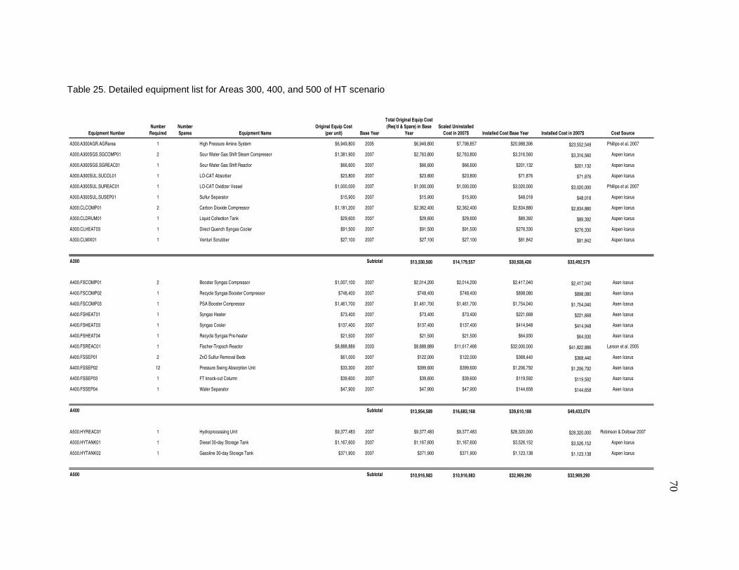
70

Table 25. Detailed equipment list for Areas 300, 400, and 500 of HT scenario

Equipment Number

Number

Required

Number

Spares Equipment Name

Original Equip Cost

(per unit) Base Year

Total Original Equip Cost

(Req'd & Spare) in Base

Year

Scaled Uninstalled

Cost in 2007$ Installed Cost Base Year Installed Cost in 2007$ Cost Source

A300.A300AGR.AGRarea 1 High Pressure Amine System $6,949,800 2005 $6,949,800 $7,798,857 $20,988,396 $23,552,549 Phillips et al. 2007

A300.A300SGS.SGCOMP01 2 Sour Water Gas Shift Steam Compressor $1,381,900 2007 $2,763,800 $2,763,800 $3,316,560 $3,316,560 Aspen Icarus

A300.A300SGS.SGREAC01 1 Sour Water Gas Shift Reactor $66,600 2007 $66,600 $66,600 $201,132 $201,132 Aspen Icarus

A300.A300SUL.SUCOL01 1 LO-CAT Absorber $23,800 2007 $23,800 $23,800 $71,876 $71,876 Aspen Icarus

A300.A300SUL.SUREAC01 1 LO-CAT Oxidizer Vessel $1,000,000 2007 $1,000,000 $1,000,000 $3,020,000 $3,020,000 Phillips et al. 2007

A300.A300SUL.SUSEP01 1 Sulfur Separator $15,900 2007 $15,900 $15,900 $48,018 $48,018 Aspen Icarus

A300.CLCOMP01 2 Carbon Dioxide Compressor $1,181,200 2007 $2,362,400 $2,362,400 $2,834,880 $2,834,880 Aspen Icarus

A300.CLDRUM01 1 Liquid Collection Tank $29,600 2007 $29,600 $29,600 $89,392 $89,392 Aspen Icarus

A300.CLHEAT03 1 Direct Quench Syngas Cooler $91,500 2007 $91,500 $91,500 $276,330 $276,330 Aspen Icarus

A300.CLMIX01 1 Venturi Scrubber $27,100 2007 $27,100 $27,100 $81,842 $81,842 Aspen Icarus

A300 Subtotal $13,330,500 $14,179,557 $30,928,426 $33,492,579

A400.FSCOMP01 2 Booster Syngas Compressor $1,007,100 2007 $2,014,200 $2,014,200 $2,417,040 $2,417,040 Asen Icarus

A400.FSCOMP02 1 Recycle Syngas Booster Compressor $748,400 2007 $748,400 $748,400 $898,080 $898,080 Asen Icarus

A400.FSCOMP03 1 PSA Booster Compressor $1,461,700 2007 $1,461,700 $1,461,700 $1,754,040 $1,754,040 Asen Icarus

A400.FSHEAT01 1 Syngas Heater $73,400 2007 $73,400 $73,400 $221,668 $221,668 Asen Icarus

A400.FSHEAT03 1 Syngas Cooler $137,400 2007 $137,400 $137,400 $414,948 $414,948 Asen Icarus

A400.FSHEAT04 1 Recycle Syngas Pre-heater $21,500 2007 $21,500 $21,500 $64,930 $64,930 Asen Icarus

A400.FSREAC01 1 Fischer-Tropsch Reactor $8,888,889 2003 $8,888,889 $11,617,468 $32,000,000 $41,822,886 Larson et al. 2005

A400.FSSEP01 2 ZnO Sulfur Removal Beds $61,000 2007 $122,000 $122,000 $368,440 $368,440 Asen Icarus

A400.FSSEP02 12 Pressure Swing Absorption Unit $33,300 2007 $399,600 $399,600 $1,206,792 $1,206,792 Asen Icarus

A400.FSSEP03 1 FT knock-out Column $39,600 2007 $39,600 $39,600 $119,592 $119,592 Asen Icarus

A400.FSSEP04 1 Water Separator $47,900 2007 $47,900 $47,900 $144,658 $144,658 Asen Icarus

A400 Subtotal $13,954,589 $16,683,168 $39,610,188 $49,433,074

A500.HYREAC01 1 Hydroprocessing Unit $9,377,483 2007 $9,377,483 $9,377,483 $28,320,000 $28,320,000 Robinson & Dolbear 2007

A500.HYTANK01 1 Diesel 30-day Storage Tank $1,167,600 2007 $1,167,600 $1,167,600 $3,526,152 $3,526,152 Aspen Icarus

A500.HYTANK02 1 Gasoline 30-day Storage Tank $371,900 2007 $371,900 $371,900 $1,123,138 $1,123,138 Aspen Icarus

A500 Subtotal $10,916,983 $10,916,983 $32,969,290 $32,969,290

71

Table 26. Detailed equipment list for Areas 600 and 700 of HT scenario

Equipment Number

Number

Required

Number

Spares Equipment Name

Original Equip Cost

(per unit) Base Year

Total Original Equip Cost

(Req'd & Spare) in Base

Year

Scaled Uninstalled

Cost in 2007$ Installed Cost Base Year Installed Cost in 2007$ Cost Source

A600.COMBB 1 Combustion Turbine - Electric Generator $22,404,000 2007 $22,404,000 $22,404,000 $26,884,800 $26,884,800 Aspen Icarus

A600.CWPUMP 1 1 Cooling Water Pump $5,900 2007 $11,800 $11,800 $35,636 $35,636 Aspen Icarus

A600.ECON1_HRSG 1 Heat Recovery Steam Generator $202,200 2007 $202,200 $202,200 $610,644 $610,644 Aspen Icarus

A600.HPPUMP 1 1 High Pressure Steam Pump $266,700 2007 $533,400 $533,400 $1,610,868 $1,610,868 Aspen Icarus

A600.HPSEP 1 High Pressure Steam/Water Separation $107,400 2007 $107,400 $107,400 $324,348 $324,348 Aspen Icarus

A600.LPEXP_ELECGEN 1 Combined Steam Turbine - Electric Gen. $4,709,600 2007 $4,709,600 $4,709,600 $5,651,520 $5,651,520 Aspen Icarus

A600.LPSEP 1 Low Pressure Water/Steam Separation $108,800 2007 $108,800 $108,800 $328,576 $328,576 Aspen Icarus

A600.O2COMP 1 Air Compressor $8,431,900 2007 $8,431,900 $8,431,900 $10,118,280 $10,118,280 Aspen Icarus

A600 Subtotal $36,509,100 $36,509,100 $45,564,672 $45,564,672

A700.COMP1 2 Air Compressor $3,346,500 2007 $6,693,000 $6,693,000 $8,031,600 $8,031,600 Aspen Icarus

A700.COOLER 1 Air Cooler $27,200 2007 $27,200 $27,200 $82,144 $82,144 Aspen Icarus

A700.GOXCLR-1 1 Oxygen Compressor Cooler $23,300 2007 $23,300 $23,300 $70,366 $70,366 Aspen Icarus

A700.GOXCLR-2 1 Oxygen Compressor Cooler $23,000 2007 $23,000 $23,000 $69,460 $69,460 Aspen Icarus

A700.GOXCMP-1 2 Oxygen Compressor $1,489,600 2007 $2,979,200 $2,979,200 $3,575,040 $3,575,040 Aspen Icarus

A700.HIGH-P.cond 1 High Pressure Column Condenser $20,300 2007 $20,300 $20,300 $61,306 $61,306 Aspen Icarus

A700.HIGH-P.cond acc 1 High Pressure Column Condenser Accumulator $40,500 2007 $40,500 $40,500 $122,310 $122,310 Aspen Icarus

A700.HIGH-P.reflux pump 1 1 High Pressure Column Reflux Pump $14,300 2007 $28,600 $28,600 $86,372 $86,372 Aspen Icarus

A700.HIGH-P.tower 1 High Pressure Column Tower $314,300 2007 $314,300 $314,300 $949,186 $949,186 Aspen Icarus

A700.INTRC1 1 Air Compressor Intercooler $338,300 2007 $338,300 $338,300 $1,021,666 $1,021,666 Aspen Icarus

A700.INTRC2 1 Air Compressor Intercooler $304,500 2007 $304,500 $304,500 $919,590 $919,590 Aspen Icarus

A700.INTRC3 1 Air Compressor Intercooler $222,500 2007 $222,500 $222,500 $671,950 $671,950 Aspen Icarus

A700.LOW-P.reb 1 Low Pressure Column Reboiler $19,600 2007 $19,600 $19,600 $59,192 $59,192 Aspen Icarus

A700.LOW-P.tower 1 Low Pressure Column Tower $2,581,600 2007 $2,581,600 $2,581,600 $7,796,432 $7,796,432 Aspen Icarus

A700.TSA 1 Water Knock-out Drum $35,900 2007 $35,900 $35,900 $108,418 $108,418 Aspen Icarus

A700.TURB-1 2 Gas Expander $86,100 2007 $172,200 $172,200 $520,044 $520,044 Aspen Icarus

A700.WK01 1 Water Knock-out Drum $57,700 2007 $57,700 $57,700 $174,254 $174,254 Aspen Icarus

A700 Subtotal $13,881,700 $13,881,700 $24,319,330 $24,319,330

$124,691,733 $130,083,951 $259,998,390 $276,233,779

$139,654,741 $145,694,026 $291,198,196 $309,381,833

Total

Total (with BOP)

72

B.3 Low Temperature Equipment List

Table 27. Detailed equipment list for Areas 100 and 200 of LT scenario

Equipment Number

Number

Required

Number

Spares Equipment Name

Original Equip Cost

(per unit) in Base Year Base Year

Total Original Equip Cost

(Req'd & Spare) in Base

Year

Scaled Uninstalled

Cost in 2007$ Installed Cost Base Year Installed Cost in 2007$ Cost Source

A100.CONV1 2 Bale Transport Conveyor $400,000 2000 $800,000 $1,066,531 $1,296,000 $1,727,781 Aden et al. 2002

A100.CONV2 2 Bale Unwrapping Conveyor $150,000 2000 $300,000 $399,949 $357,000 $475,940 Aden et al. 2002

A100.CONV3 1 Belt Press Discharge Conveyor $50,000 2000 $50,000 $66,658 $94,500 $125,984 Aden et al. 2002

A100.SCALE 2 Truck Scales $34,000 2000 $68,000 $90,655 $167,960 $223,918 Aden et al. 2002

A100.FORK1 4 1 Truck Unloading Forklift $18,000 2000 $90,000 $119,985 $90,000 $119,985 Aden et al. 2002

A100.FORK2 4 Bale Moving Forklift $18,000 2000 $72,000 $95,988 $72,000 $95,988 Aden et al. 2002

A100.SLAB 1 Concrete Feedstock-Storage Slab $450,655 2000 $450,655 $600,797 $991,441 $1,321,754 Aden et al. 2002

A100.MAGSEP 1 Magnetic Separator $13,863 1998 $13,863 $18,700 $18,022 $24,310 Aden et al. 2002

A100.A100CHOP.CHGRIN01 4 Chopper $105,100 2007 $420,400 $420,400 $1,105,258 $1,105,258 Aspen Icarus

A100.A100CHOP.CHMIX01 1 Chopper Conveyor $61,400 2007 $61,400 $61,400 $185,428 $185,428 Aspen Icarus

A100.A100CHOP.CHSEP01 1 Chopper Screen with Recycle Conveyor $20,800 2007 $20,800 $20,800 $62,816 $62,816 Aspen Icarus

A100.A100DRY.DRDRY01 10 Dryer $633,700 2007 $6,337,000 $6,337,000 $15,201,647 $15,201,647 Aspen Icarus

A100.A100GRIN.GRGRIN01 4 Grinder $167,100 2007 $668,400 $668,400 $1,757,266 $1,757,266 Aspen Icarus

A100.A100GRIN.GRMIX01 1 Grinder Conveyor $61,400 2007 $61,400 $61,400 $185,428 $185,428 Aspen Icarus

A100.A100GRIN.GRSEP01 1 Grinder Screen with Recycle Conveyor $20,800 2007 $20,800 $20,800 $62,816 $62,816 Aspen Icarus

A100 Subtotal $9,434,718 $10,049,464 $21,647,582 $22,676,317

A200.A200COMB.CBCYC01 3 Combustor Cyclone (medium efficiency) $35,400 2007 $106,200 $106,200 $320,724 $320,724 Aspen Icarus

A200.A200COMB.CBCYC02 3 Combustor Cyclone (high efficiency) $6,700 2007 $20,100 $20,100 $60,702 $60,702 Aspen Icarus

A200.A200COMB.CBMIX01 1 Ash Storage Vessel $142,800 2007 $142,800 $142,800 $431,256 $431,256 Aspen Icarus

A200.A200COMB.CBREAC01 1 Combustor - Steam Boiler $1,450,500 2007 $1,450,500 $1,450,500 $4,380,510 $4,380,510 Aspen Icarus

A200.A200CYC.CYCYC01 2 1st train, medium efficiency cyclone $20,300 2007 $40,600 $40,600 $122,612 $122,612 Aspen Icarus

A200.A200CYC.CYCYC02 4 1st train, high efficiency cyclone $24,900 2007 $99,600 $99,600 $300,792 $300,792 Aspen Icarus

A200.A200CYC.CYMIX02 1 Char Collector and conveyor $84,400 2007 $84,400 $84,400 $254,888 $254,888 Aspen Icarus

A200.GSREAC01 7 Fluidized Bed Gasifier (Pressurized) $1,096,170 2003 $7,673,191 $10,028,594 $14,843,424 $19,399,838 Larson et al. 2005

A200.GSTANK01 7 Biomass Receiving Hopper $71,700 2007 $501,900 $501,900 $1,247,712 $1,247,712 Aspen Icarus

A200.GSTANK02 7 Lockhopper $47,700 2007 $333,900 $333,900 $830,068 $830,068 Aspen Icarus

A200.GSTANK03 7 Biomass Feeding Bin $47,700 2007 $333,900 $333,900 $830,068 $830,068 Aspen Icarus

A200 Subtotal $10,787,091 $13,142,494 $23,622,756 $28,179,170

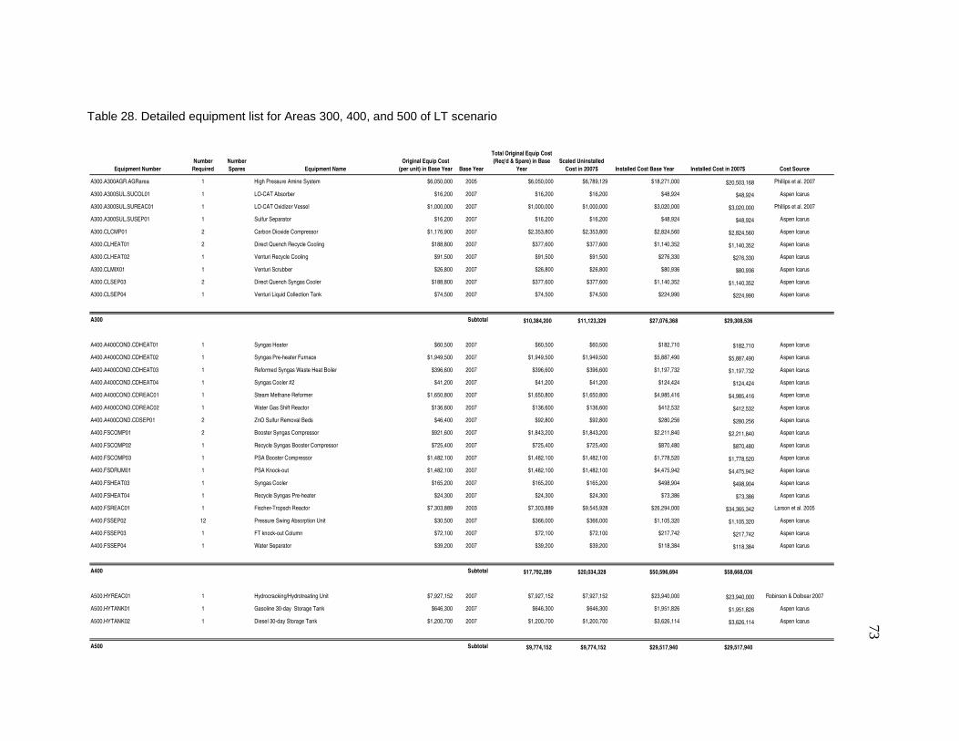
73

Table 28. Detailed equipment list for Areas 300, 400, and 500 of LT scenario

Equipment Number

Number

Required

Number

Spares Equipment Name

Original Equip Cost

(per unit) in Base Year Base Year

Total Original Equip Cost

(Req'd & Spare) in Base

Year

Scaled Uninstalled

Cost in 2007$ Installed Cost Base Year Installed Cost in 2007$ Cost Source

A300.A300AGR.AGRarea 1 High Pressure Amine System $6,050,000 2005 $6,050,000 $6,789,129 $18,271,000 $20,503,168 Phillips et al. 2007

A300.A300SUL.SUCOL01 1 LO-CAT Absorber $16,200 2007 $16,200 $16,200 $48,924 $48,924 Aspen Icarus

A300.A300SUL.SUREAC01 1 LO-CAT Oxidizer Vessel $1,000,000 2007 $1,000,000 $1,000,000 $3,020,000 $3,020,000 Phillips et al. 2007

A300.A300SUL.SUSEP01 1 Sulfur Separator $16,200 2007 $16,200 $16,200 $48,924 $48,924 Aspen Icarus

A300.CLCMP01 2 Carbon Dioxide Compressor $1,176,900 2007 $2,353,800 $2,353,800 $2,824,560 $2,824,560 Aspen Icarus

A300.CLHEAT01 2 Direct Quench Recycle Cooling $188,800 2007 $377,600 $377,600 $1,140,352 $1,140,352 Aspen Icarus

A300.CLHEAT02 1 Venturi Recycle Cooling $91,500 2007 $91,500 $91,500 $276,330 $276,330 Aspen Icarus

A300.CLMIX01 1 Venturi Scrubber $26,800 2007 $26,800 $26,800 $80,936 $80,936 Aspen Icarus

A300.CLSEP03 2 Direct Quench Syngas Cooler $188,800 2007 $377,600 $377,600 $1,140,352 $1,140,352 Aspen Icarus

A300.CLSEP04 1 Venturi Liquid Collection Tank $74,500 2007 $74,500 $74,500 $224,990 $224,990 Aspen Icarus

A300 Subtotal $10,384,200 $11,123,329 $27,076,368 $29,308,536

A400.A400COND.CDHEAT01 1 Syngas Heater $60,500 2007 $60,500 $60,500 $182,710 $182,710 Aspen Icarus

A400.A400COND.CDHEAT02 1 Syngas Pre-heater Furnace $1,949,500 2007 $1,949,500 $1,949,500 $5,887,490 $5,887,490 Aspen Icarus

A400.A400COND.CDHEAT03 1 Reformed Syngas Waste Heat Boiler $396,600 2007 $396,600 $396,600 $1,197,732 $1,197,732 Aspen Icarus

A400.A400COND.CDHEAT04 1 Syngas Cooler #2 $41,200 2007 $41,200 $41,200 $124,424 $124,424 Aspen Icarus

A400.A400COND.CDREAC01 1 Steam Methane Reformer $1,650,800 2007 $1,650,800 $1,650,800 $4,985,416 $4,985,416 Aspen Icarus

A400.A400COND.CDREAC02 1 Water Gas Shift Reactor $136,600 2007 $136,600 $136,600 $412,532 $412,532 Aspen Icarus

A400.A400COND.CDSEP01 2 ZnO Sulfur Removal Beds $46,400 2007 $92,800 $92,800 $280,256 $280,256 Aspen Icarus

A400.FSCOMP01 2 Booster Syngas Compressor $921,600 2007 $1,843,200 $1,843,200 $2,211,840 $2,211,840 Aspen Icarus

A400.FSCOMP02 1 Recycle Syngas Booster Compressor $725,400 2007 $725,400 $725,400 $870,480 $870,480 Aspen Icarus

A400.FSCOMP03 1 PSA Booster Compressor $1,482,100 2007 $1,482,100 $1,482,100 $1,778,520 $1,778,520 Aspen Icarus

A400.FSDRUM01 1 PSA Knock-out $1,482,100 2007 $1,482,100 $1,482,100 $4,475,942 $4,475,942 Aspen Icarus

A400.FSHEAT03 1 Syngas Cooler $165,200 2007 $165,200 $165,200 $498,904 $498,904 Aspen Icarus

A400.FSHEAT04 1 Recycle Syngas Pre-heater $24,300 2007 $24,300 $24,300 $73,386 $73,386 Aspen Icarus

A400.FSREAC01 1 Fischer-Tropsch Reactor $7,303,889 2003 $7,303,889 $9,545,928 $26,294,000 $34,365,342 Larson et al. 2005

A400.FSSEP02 12 Pressure Swing Absorption Unit $30,500 2007 $366,000 $366,000 $1,105,320 $1,105,320 Aspen Icarus

A400.FSSEP03 1 FT knock-out Column $72,100 2007 $72,100 $72,100 $217,742 $217,742 Aspen Icarus

A400.FSSEP04 1 Water Separator $39,200 2007 $39,200 $39,200 $118,384 $118,384 Aspen Icarus

A400 Subtotal $17,792,289 $20,034,328 $50,596,694 $58,668,036

A500.HYREAC01 1 Hydrocracking/Hydrotreating Unit $7,927,152 2007 $7,927,152 $7,927,152 $23,940,000 $23,940,000 Robinson & Dolbear 2007

A500.HYTANK01 1 Gasoline 30-day Storage Tank $646,300 2007 $646,300 $646,300 $1,951,826 $1,951,826 Aspen Icarus

A500.HYTANK02 1 Diesel 30-day Storage Tank $1,200,700 2007 $1,200,700 $1,200,700 $3,626,114 $3,626,114 Aspen Icarus

A500 Subtotal $9,774,152 $9,774,152 $29,517,940 $29,517,940

74

Table 29. Detailed equipment list for Areas 600 and 700 of LT scenario

Equipment Number

Number

Required

Number

Spares Equipment Name

Original Equip Cost

(per unit) in Base Year Base Year

Total Original Equip Cost

(Req'd & Spare) in Base

Year

Scaled Uninstalled

Cost in 2007$ Installed Cost Base Year Installed Cost in 2007$ Cost Source

A600.COMBB 1 Combustion Turbine - Electric Generator $18,607,700 2007 $18,607,700 $18,607,700 $22,329,240 $22,329,240 Aspen Icarus

A600.CWPUMP 1 1 Cooling Water Pump $5,900 2007 $11,800 $11,800 $35,636 $35,636 Aspen Icarus

A600.ECON1_HRSG 1 Heat Recovery Steam Generator $202,200 2007 $202,200 $202,200 $610,644 $610,644 Aspen Icarus

A600.HPPUMP 1 1 High Pressure Steam Pump $266,700 2007 $533,400 $533,400 $1,610,868 $1,610,868 Aspen Icarus

A600.HPSEP 1 High Pressure Steam/Water Separation $107,400 2007 $107,400 $107,400 $324,348 $324,348 Aspen Icarus

A600.LPEXP_ELECGEN 1 Combined Steam Turbine - Electric Gen. $5,056,300 2007 $5,056,300 $5,056,300 $6,067,560 $6,067,560 Aspen Icarus

A600.LPSEP 1 Low Pressure Water/Steam Separation $108,800 2007 $108,800 $108,800 $328,576 $328,576 Aspen Icarus

A600.O2COMP 1 Air Compressor $6,331,200 2007 $6,331,200 $6,331,200 $7,597,440 $7,597,440 Aspen Icarus

A600 Subtotal $30,958,800 $30,958,800 $38,904,312 $38,904,312

A700.COMP1 2 Air Compressor $3,119,600 2007 $6,239,200 $6,239,200 $7,487,040 $7,487,040 Aspen Icarus

A700.COOLER 1 Air Cooler $24,300 2007 $24,300 $24,300 $73,386 $73,386 Aspen Icarus

A700.GOXCLR-1 1 Oxygen Compressor Cooler $23,300 2007 $23,300 $23,300 $70,366 $70,366 Aspen Icarus

A700.GOXCLR-2 1 Oxygen Compressor Cooler $23,000 2007 $23,000 $23,000 $69,460 $69,460 Aspen Icarus

A700.GOXCMP-1 2 Oxygen Compressor $1,514,700 2007 $3,029,400 $3,029,400 $3,635,280 $3,635,280 Aspen Icarus

A700.HIGH-P.cond 1 High Pressure Column Condenser $20,300 2007 $20,300 $20,300 $61,306 $61,306 Aspen Icarus

A700.HIGH-P.cond acc 1 High Pressure Column Condenser Accumulator $36,300 2007 $36,300 $36,300 $109,626 $109,626 Aspen Icarus

A700.HIGH-P.reflux pump 1 1 High Pressure Column Reflux Pump $14,300 2007 $28,600 $28,600 $34,320 $34,320 Aspen Icarus

A700.HIGH-P.tower 1 High Pressure Column Tower $279,900 2007 $279,900 $279,900 $335,880 $335,880 Aspen Icarus

A700.INTRC1 1 Air Compressor Intercooler $338,300 2007 $338,300 $338,300 $405,960 $405,960 Aspen Icarus

A700.INTRC2 1 Air Compressor Intercooler $304,500 2007 $304,500 $304,500 $919,590 $919,590 Aspen Icarus

A700.INTRC3 1 Air Compressor Intercooler $222,500 2007 $222,500 $222,500 $671,950 $671,950 Aspen Icarus

A700.LOW-P.reb 2 Low Pressure Column Reboiler $19,600 2007 $39,200 $39,200 $118,384 $118,384 Aspen Icarus

A700.LOW-P.tower 1 Low Pressure Column Tower $1,538,900 2007 $1,538,900 $1,538,900 $4,647,478 $4,647,478 Aspen Icarus

A700.TSA 1 Water Knock-out Drum $30,100 2007 $30,100 $30,100 $90,902 $90,902 Aspen Icarus

A700.TURB-1 2 Gas Expander $89,200 2007 $178,400 $178,400 $538,768 $538,768 Aspen Icarus

A700.WK01 1 Water Knock-out Drum $64,800 2007 $64,800 $64,800 $195,696 $195,696 Aspen Icarus

A700 Subtotal $12,421,000 $12,421,000 $19,465,392 $19,465,392

Total $101,552,251 $107,503,567 $210,831,043 $226,719,704

Total (with BOP) $113,738,521 $120,403,995 $236,130,768 $253,926,068

75

B.4 Discounted Cash Flow

B.4.1 High Temperature Scenario

Table 30. Discounted cash flow sheet for construction period and years 1-8 of HT scenario

DCFROR WorksheetDCFROR WorksheetDCFROR WorksheetDCFROR Worksheet

Year -2 -1 0 1 2 3 4 5 6 7 8

Fixed Capital Investment $50,890,395 $316,115,651 $168,595,014

Working Capital $79,028,913

Loan Payment $0 $0 $0 $0 $0 $0 $0 $0

Loan Interest Payment $0 $0 $0 $0 $0 $0 $0 $0 $0 $0 $0

Loan Principal $0 $0 $0 $0 $0 $0 $0 $0 $0 $0 $0

GGE (Gallon of Gasoline Equiv.) Sales $133,364,635 $177,819,513 $177,819,513 $177,819,513 $177,819,513 $177,819,513 $177,819,513 $177,819,513

Diesel Sales $0 $0 $0 $0 $0 $0 $0 $0 By-Product Credit $4,173,208 $5,564,277 $5,564,277 $5,564,277 $5,564,277 $5,564,277 $5,564,277 $5,564,277Plant Performance 1.00 1.00 1.00 1.00 1.00 1.00 1.00 1.00

Total Annual Sales $137,537,843 $183,383,791 $183,383,791 $183,383,791 $183,383,791 $183,383,791 $183,383,791 $183,383,791

Annual Manufacturing Cost

Raw Materials $44,894,145 $51,307,594 $51,307,594 $51,307,594 $51,307,594 $51,307,594 $51,307,594 $51,307,594

SWGS catalysts $114,621 $0 $0 $114,621 $0 $0 $114,621 $0

Steam reforming catalysts $0 $0 $0 $0 $0 $0 $0 $0

ZnO $424,410 $0 $0 $424,410 $0 $0 $424,410 $0

Pressure Swing Adsorption Packing $497,135 $0 $0 $497,135 $0 $0 $497,135 $0

FT catalysts $7,686,720 $0 $0 $7,686,720 $0 $0 $7,686,720 $0

Other Variable Costs $11,727,856 $13,403,264 $13,403,264 $13,403,264 $13,403,264 $13,403,264 $13,403,264 $13,403,264

Fixed Operating Costs $14,345,785 $14,345,785 $14,345,785 $14,345,785 $14,345,785 $14,345,785 $14,345,785 $14,345,785

Total Product Cost $79,690,672 $79,056,643 $79,056,643 $87,779,529 $79,056,643 $79,056,643 $87,779,529 $79,056,643

Annual Depreciation

General Plant

DDB $128,361,546 $91,686,818 $65,490,585 $46,778,989 $33,413,564 $23,866,831 $17,047,737

SL $64,180,773 $53,483,977 $45,843,409 $40,931,615 $38,982,491 $38,982,491 $38,982,491

Remaining Value $320,903,864 $229,217,046 $163,726,461 $116,947,472 $83,533,909 $59,667,078 $42,619,341

Actual $128,361,546 $91,686,818 $65,490,585 $46,778,989 $38,982,491 $38,982,491 $38,982,491

Steam Plant

DDB $5,819,551 $5,383,084 $4,979,353 $4,605,902 $4,260,459 $3,940,925 $3,645,355 $3,371,954

SL $3,879,700 $3,777,603 $3,688,410 $3,612,472 $3,550,382 $3,503,044 $3,471,767 $3,458,414

Remaining Value $71,774,458 $66,391,374 $61,412,021 $56,806,119 $52,545,660 $48,604,736 $44,959,380 $41,587,427

Actual $5,819,551 $5,383,084 $4,979,353 $4,605,902 $4,260,459 $3,940,925 $3,645,355 $3,458,414

Net Revenue ($76,333,925) $7,257,245 $33,857,210 $44,219,371 $61,084,198 $61,403,732 $52,976,416 $100,868,733

Losses Forward ($76,333,925) ($69,076,681) ($35,219,471) $0 $0 $0 $0

Taxable Income ($76,333,925) ($69,076,681) ($35,219,471) $8,999,900 $61,084,198 $61,403,732 $52,976,416 $100,868,733

Income Tax $0 $0 $0 $3,509,961 $23,822,837 $23,947,455 $20,660,802 $39,338,806

Annual Cash Income $57,847,171 $104,327,147 $104,327,147 $92,094,301 $80,504,310 $80,379,692 $74,943,459 $64,988,341

Discount Factor 1.21 1.1 1 0.909090909 0.826446281 0.751314801 0.683013455 0.620921323 0.56447393 0.513158118 0.46650738

Annual Present Value $645,181,377 $52,588,337 $86,220,783 $78,382,530 $62,901,646 $49,986,843 $45,372,241 $38,457,845 $30,317,541

Total Capital Investment + Interest $61,577,378 $347,727,216 $247,623,927

Net Present Worth $0

76

Table 31. Discounted cash flow sheet for years 9-20 of HT scenario

DCFROR WorksheetDCFROR WorksheetDCFROR WorksheetDCFROR Worksheet

Year 9 10 11 12 13 14 15 16 17 18 19 20

Fixed Capital Investment

Working Capital ($79,028,913)

Loan Payment $0 $0 $0 $0 $0 $0 $0 $0 $0 $0 $0 $0

Loan Interest Payment $0 $0 $0 $0 $0 $0 $0 $0 $0 $0 $0 $0

Loan Principal $0 $0 $0 $0 $0 $0 $0 $0 $0 $0 $0 $0

GGE (Gallon of Gasoline Equiv.) Sales $177,819,513 $177,819,513 $177,819,513 $177,819,513 $177,819,513 $177,819,513 $177,819,513 $177,819,513 $177,819,513 $177,819,513 $177,819,513 $177,819,513

Diesel Sales $0 $0 $0 $0 $0 $0 $0 $0 $0 $0 $0 $0 By-Product Credit $5,564,277 $5,564,277 $5,564,277 $5,564,277 $5,564,277 $5,564,277 $5,564,277 $5,564,277 $5,564,277 $5,564,277 $5,564,277 $5,564,277Plant Performance 1.00 1.00 1.00 1.00 1.00 1.00 1.00 1.00 1.00 1.00 1.00 1.00

Total Annual Sales $183,383,791 $183,383,791 $183,383,791 $183,383,791 $183,383,791 $183,383,791 $183,383,791 $183,383,791 $183,383,791 $183,383,791 $183,383,791 $183,383,791

Annual Manufacturing Cost

Raw Materials $51,307,594 $51,307,594 $51,307,594 $51,307,594 $51,307,594 $51,307,594 $51,307,594 $51,307,594 $51,307,594 $51,307,594 $51,307,594 $51,307,594

SWGS catalysts $0 $114,621 $0 $0 $114,621 $0 $0 $114,621 $0 $0 $114,621 $0

Steam reforming catalysts $0 $0 $0 $0 $0 $0 $0 $0 $0 $0 $0 $0

ZnO $0 $424,410 $0 $0 $424,410 $0 $0 $424,410 $0 $0 $424,410 $0

Pressure Swing Adsorption Packing $0 $497,135 $0 $0 $497,135 $0 $0 $497,135 $0 $0 $497,135 $0

FT catalysts $0 $7,686,720 $0 $0 $7,686,720 $0 $0 $7,686,720 $0 $0 $7,686,720 $0

Other Variable Costs $13,403,264 $13,403,264 $13,403,264 $13,403,264 $13,403,264 $13,403,264 $13,403,264 $13,403,264 $13,403,264 $13,403,264 $13,403,264 $13,403,264

Fixed Operating Costs $14,345,785 $14,345,785 $14,345,785 $14,345,785 $14,345,785 $14,345,785 $14,345,785 $14,345,785 $14,345,785 $14,345,785 $14,345,785 $14,345,785

Total Product Cost $79,056,643 $87,779,529 $79,056,643 $79,056,643 $87,779,529 $79,056,643 $79,056,643 $87,779,529 $79,056,643 $79,056,643 $87,779,529 $79,056,643

Annual Depreciation

General Plant

DDB

SL

Remaining Value

Actual

Steam Plant

DDB $3,119,057 $2,885,128 $2,668,743 $2,468,587 $2,283,443 $2,112,185 $1,953,771 $1,807,238 $1,671,696 $1,546,318 $1,430,344 $1,323,069

SL $3,458,414 $3,458,414 $3,458,414 $3,458,414 $3,458,414 $3,458,414 $3,458,414 $3,458,414 $3,458,414 $3,458,414 $3,458,414 $3,458,414

Remaining Value $38,468,370 $35,583,242 $32,914,499 $30,445,912 $28,162,468 $26,050,283 $24,096,512 $22,289,273 $20,617,578 $19,071,260 $17,640,915 $16,317,847

Actual $3,458,414 $3,458,414 $3,458,414 $3,458,414 $3,458,414 $3,458,414 $3,458,414 $3,458,414 $3,458,414 $3,458,414 $3,458,414 $3,458,414

Net Revenue $100,868,733 $92,145,848 $100,868,733 $100,868,733 $92,145,848 $100,868,733 $100,868,733 $92,145,848 $100,868,733 $100,868,733 $92,145,848 $100,868,733

Losses Forward $0 $0 $0 $0 $0 $0 $0 $0 $0 $0 $0 $0

Taxable Income $100,868,733 $92,145,848 $100,868,733 $100,868,733 $92,145,848 $100,868,733 $100,868,733 $92,145,848 $100,868,733 $100,868,733 $92,145,848 $100,868,733

Income Tax $39,338,806 $35,936,881 $39,338,806 $39,338,806 $35,936,881 $39,338,806 $39,338,806 $35,936,881 $39,338,806 $39,338,806 $35,936,881 $39,338,806

Annual Cash Income $64,988,341 $59,667,381 $64,988,341 $64,988,341 $59,667,381 $64,988,341 $64,988,341 $59,667,381 $64,988,341 $64,988,341 $59,667,381 $64,988,341

Discount Factor 0.424097618 0.385543289 0.350493899 0.318630818 0.28966438 0.263331254 0.239392049 0.217629136 0.197844669 0.17985879 0.163507991 0.148643628

Annual Present Value $27,561,401 $23,004,358 $22,778,017 $20,707,288 $17,283,515 $17,113,461 $15,557,692 $12,985,361 $12,857,597 $11,688,724 $9,756,094 $9,660,103

Total Capital Investment + Interest ($11,747,144.32)

Net Present Worth

77

B.4.2 Low Temperature Scenario

Table 32. Discounted cash flow sheet for construction period and years 1-8 of LT scenario

DCFROR WorksheetDCFROR WorksheetDCFROR WorksheetDCFROR Worksheet

Year -2 -1 0 1 2 3 4 5 6 7 8

Fixed Capital Investment $41,888,460 $259,981,649 $138,656,880

Working Capital $64,995,412

Loan Payment $0 $0 $0 $0 $0 $0 $0 $0

Loan Interest Payment $0 $0 $0 $0 $0 $0 $0 $0 $0 $0 $0

Loan Principal $0 $0 $0 $0 $0 $0 $0 $0 $0 $0 $0

GGE (Gallon of Gasoline Equiv.) Sales $117,025,289 $156,033,719 $156,033,719 $156,033,719 $156,033,719 $156,033,719 $156,033,719 $156,033,719

Diesel Sales $0 $0 $0 $0 $0 $0 $0 $0 By-Product Credit $4,945,498 $6,593,998 $6,593,998 $6,593,998 $6,593,998 $6,593,998 $6,593,998 $6,593,998Plant Performance 1.00 1.00 1.00 1.00 1.00 1.00 1.00 1.00

Total Annual Sales $121,970,788 $162,627,717 $162,627,717 $162,627,717 $162,627,717 $162,627,717 $162,627,717 $162,627,717

Annual Manufacturing Cost

Raw Materials $44,894,145 $51,307,594 $51,307,594 $51,307,594 $51,307,594 $51,307,594 $51,307,594 $51,307,594

WGS catalysts $104,732 $0 $0 $104,732 $0 $0 $104,732 $0

Steam reforming catalysts $103,412 $0 $0 $103,412 $0 $0 $103,412 $0

ZnO $424,410 $0 $0 $424,410 $0 $0 $424,410 $0

Pressure Swing Adsorption Packing $497,135 $0 $0 $497,135 $0 $0 $497,135 $0

FT catalysts $6,127,680 $0 $0 $6,127,680 $0 $0 $6,127,680 $0

Other Variable Costs $11,238,097 $12,843,539 $12,843,539 $12,843,539 $12,843,539 $12,843,539 $12,843,539 $12,843,539

Fixed Operating Costs $12,404,834 $12,404,834 $12,404,834 $12,404,834 $12,404,834 $12,404,834 $12,404,834 $12,404,834

Total Product Cost $75,794,444 $76,555,967 $76,555,967 $83,813,336 $76,555,967 $76,555,967 $83,813,336 $76,555,967

Annual Depreciation

General Plant

DDB $104,833,121 $74,880,801 $53,486,286 $38,204,490 $27,288,922 $19,492,087 $13,922,919

SL $52,416,561 $43,680,467 $37,440,400 $33,428,929 $31,837,075 $31,837,075 $31,837,075

Remaining Value $262,082,803 $187,202,002 $133,715,716 $95,511,226 $68,222,304 $48,730,217 $34,807,298

Actual $104,833,121 $74,880,801 $53,486,286 $38,204,490 $31,837,075 $31,837,075 $31,837,075

Steam Plant

DDB $4,979,012 $4,605,586 $4,260,167 $3,940,654 $3,645,105 $3,371,722 $3,118,843 $2,884,930

SL $3,319,341 $3,231,990 $3,155,679 $3,090,709 $3,037,588 $2,997,087 $2,970,327 $2,958,903

Remaining Value $61,407,813 $56,802,227 $52,542,060 $48,601,405 $44,956,300 $41,584,577 $38,465,734 $35,580,804

Actual $4,979,012 $4,605,586 $4,260,167 $3,940,654 $3,645,105 $3,371,722 $3,118,843 $2,958,903

Net Revenue ($63,635,790) $6,585,363 $28,325,297 $36,669,236 $50,589,570 $50,862,953 $43,858,462 $83,112,848

Losses Forward ($63,635,790) ($57,050,426) ($28,725,129) $0 $0 $0 $0

Taxable Income ($63,635,790) ($57,050,426) ($28,725,129) $7,944,107 $50,589,570 $50,862,953 $43,858,462 $83,112,848

Income Tax $0 $0 $0 $3,098,202 $19,729,932 $19,836,551 $17,104,800 $32,414,011

Annual Cash Income $46,176,343 $86,071,750 $86,071,750 $75,716,179 $66,341,818 $66,235,199 $61,709,581 $53,657,740

Discount Factor 1.21 1.1 1 0.909090909 0.826446281 0.751314801 0.683013455 0.620921323 0.56447393 0.513158118 0.46650738

Annual Present Value $530,655,988 $41,978,494 $71,133,678 $64,666,980 $51,715,169 $41,193,049 $37,388,043 $31,666,772 $25,031,732

Total Capital Investment + Interest $50,685,036 $285,979,814 $203,652,292

Net Present Worth $0

78

Table 33. Discounted cash flow sheet for years 9-20 of LT scenario

DCFROR WorksheetDCFROR WorksheetDCFROR WorksheetDCFROR Worksheet

Year 9 10 11 12 13 14 15 16 17 18 19 20

Fixed Capital Investment

Working Capital ($64,995,412)

Loan Payment $0 $0 $0 $0 $0 $0 $0 $0 $0 $0 $0 $0

Loan Interest Payment $0 $0 $0 $0 $0 $0 $0 $0 $0 $0 $0 $0

Loan Principal $0 $0 $0 $0 $0 $0 $0 $0 $0 $0 $0 $0

GGE (Gallon of Gasoline Equiv.) Sales $156,033,719 $156,033,719 $156,033,719 $156,033,719 $156,033,719 $156,033,719 $156,033,719 $156,033,719 $156,033,719 $156,033,719 $156,033,719 $156,033,719

Diesel Sales $0 $0 $0 $0 $0 $0 $0 $0 $0 $0 $0 $0 By-Product Credit $6,593,998 $6,593,998 $6,593,998 $6,593,998 $6,593,998 $6,593,998 $6,593,998 $6,593,998 $6,593,998 $6,593,998 $6,593,998 $6,593,998Plant Performance 1.00 1.00 1.00 1.00 1.00 1.00 1.00 1.00 1.00 1.00 1.00 1.00

Total Annual Sales $162,627,717 $162,627,717 $162,627,717 $162,627,717 $162,627,717 $162,627,717 $162,627,717 $162,627,717 $162,627,717 $162,627,717 $162,627,717 $162,627,717

Annual Manufacturing Cost

Raw Materials $51,307,594 $51,307,594 $51,307,594 $51,307,594 $51,307,594 $51,307,594 $51,307,594 $51,307,594 $51,307,594 $51,307,594 $51,307,594 $51,307,594

WGS catalysts $0 $104,732 $0 $0 $104,732 $0 $0 $104,732 $0 $0 $104,732 $0

Steam reforming catalysts $0 $103,412 $0 $0 $103,412 $0 $0 $103,412 $0 $0 $103,412 $0

ZnO $0 $424,410 $0 $0 $424,410 $0 $0 $424,410 $0 $0 $424,410 $0

Pressure Swing Adsorption Packing $0 $497,135 $0 $0 $497,135 $0 $0 $497,135 $0 $0 $497,135 $0

FT catalysts $0 $6,127,680 $0 $0 $6,127,680 $0 $0 $6,127,680 $0 $0 $6,127,680 $0

Other Variable Costs $12,843,539 $12,843,539 $12,843,539 $12,843,539 $12,843,539 $12,843,539 $12,843,539 $12,843,539 $12,843,539 $12,843,539 $12,843,539 $12,843,539

Fixed Operating Costs $12,404,834 $12,404,834 $12,404,834 $12,404,834 $12,404,834 $12,404,834 $12,404,834 $12,404,834 $12,404,834 $12,404,834 $12,404,834 $12,404,834

Total Product Cost $76,555,967 $83,813,336 $76,555,967 $76,555,967 $83,813,336 $76,555,967 $76,555,967 $83,813,336 $76,555,967 $76,555,967 $83,813,336 $76,555,967

Annual Depreciation

General Plant

DDB

SL

Remaining Value

Actual

Steam Plant

DDB $2,668,560 $2,468,418 $2,283,287 $2,112,040 $1,953,637 $1,807,115 $1,671,581 $1,546,212 $1,430,246 $1,322,978 $1,223,755 $1,131,973

SL $2,958,903 $2,958,903 $2,958,903 $2,958,903 $2,958,903 $2,958,903 $2,958,903 $2,958,903 $2,958,903 $2,958,903 $2,958,903 $2,958,903

Remaining Value $32,912,244 $30,443,825 $28,160,538 $26,048,498 $24,094,861 $22,287,746 $20,616,165 $19,069,953 $17,639,706 $16,316,728 $15,092,974 $13,961,001

Actual $2,958,903 $2,958,903 $2,958,903 $2,958,903 $2,958,903 $2,958,903 $2,958,903 $2,958,903 $2,958,903 $2,958,903 $2,958,903 $2,958,903

Net Revenue $83,112,848 $75,855,478 $83,112,848 $83,112,848 $75,855,478 $83,112,848 $83,112,848 $75,855,478 $83,112,848 $83,112,848 $75,855,478 $83,112,848

Losses Forward $0 $0 $0 $0 $0 $0 $0 $0 $0 $0 $0 $0

Taxable Income $83,112,848 $75,855,478 $83,112,848 $83,112,848 $75,855,478 $83,112,848 $83,112,848 $75,855,478 $83,112,848 $83,112,848 $75,855,478 $83,112,848

Income Tax $32,414,011 $29,583,637 $32,414,011 $32,414,011 $29,583,637 $32,414,011 $32,414,011 $29,583,637 $32,414,011 $32,414,011 $29,583,637 $32,414,011

Annual Cash Income $53,657,740 $49,230,744 $53,657,740 $53,657,740 $49,230,744 $53,657,740 $53,657,740 $49,230,744 $53,657,740 $53,657,740 $49,230,744 $53,657,740

Discount Factor 0.424097618 0.385543289 0.350493899 0.318630818 0.28966438 0.263331254 0.239392049 0.217629136 0.197844669 0.17985879 0.163507991 0.148643628

Annual Present Value $22,756,120 $18,980,583 $18,806,710 $17,097,009 $14,260,393 $14,129,760 $12,845,236 $10,714,044 $10,615,898 $9,650,816 $8,049,620 $7,975,881

Total Capital Investment + Interest ($9,661,153.89)

Net Present Worth

79

B.5 Pioneer Plant Analysis Details

Variables used in determining pioneer plant performance (equation 17).

NEWSTEPS (0+): The feedstock handling area was chosen as a new step because of the large scale which has not been demonstrated with biomass. The gasifier and solids feeding are also included as a new step because a pressurized biomass feeding system has not been demonstrated at a commercial scale except for limited campaigns.

BALEQS (0 to 100): The mass and energy balances cannot be validated with current plant data, so a value of zero is chosen.

WASTE (0 to 5): Waste streams for gasification include scrubber sludge, black water, gasifier slag, fly ash, and sulfur. The scrubber sludge and black water requires chemical treatment and the sulfur requires special handling. A mid-range value of is 2.5 chosen.

SOLIDS (0 or 1): Solids are present, therefore a value of 1 is used.

Variables used in determining pioneer plant cost growth (equation 16).

PCTNEW (0 to 100%): The percentage cost of the gasifier, solids pressurizing, and solids feeding out of the total purchased equipment cost.

IMPURITIES (0 to 5): There are two major recycle streams in the gasification process, and there is the possibility of inert component buildup. There is also a potential for equipment corrosion due to sulfur components, hydrogen chloride, and hydrogen, so a value of 4 is assigned.

COMPLEXITY (0+): There are 9 continuously linked steps in the gasification process. These include feedstock handling, solids feeding, gasification, amine scrubbing, sour water-gas-shift, pressure swing adsorption, Fischer-Tropsch synthesis, hydroprocessing, and air separation.

INCLUSIVENESS (0 to 100): Land costs and startup costs are considered in the TCI, however, they have not been rigorously investigated. A value of 33% is used.

PROJECT DEFINITION (2 to 8): The gasification platform is considered to be in the study

design stage so a value of 7 was assigned.

80

Table 34. Pioneer plant analysis parameters and factors

Parameter Baseline Optimistic Pessimistic Range

NEWSTEPS 2 1 3 0+

BALEQS 0 0 0 0-100

WASTE 4 3 5 0-5

SOLIDS 1 1 1 0 or 1

Plant Perf. 38.18 49.93 22.31 0-100

PCTNEW 19 (9)a 10 (5)a 25 (20)a 0-100

IMPURITIES 4 3 5 0-5

COMPLEX 9 6 12 0+

INCLUSIV. 33 50 0 0-100

PROJ. DEF. 7 6 8 2-8

Cost Growth(HT) 0.47 0.63 0.30 0-1

Cost Growth(LT) 0.50 0.65 0.31 0-1

(a) value in parentheses is value chosen for LT scenario

81

APPENDIX C. SCENARIO MODELING DETAILS

C.1 Property Method

The model setup includes a particle size distribution in order to better estimate the solids simulation in the grinding and cyclone operations. It operates globally with the Redlich-Kwong-Soave with Boston-Mathias modification (RKS-BM) property method which is recommended for medium temperature refining and gas processing operations including combustion and gasification. During acid gas absorption and stripping another property method, ELECNRTL, is used for more accurate simulation. The solids handling such as in the pretreatment area and cyclones, the SOLIDS property method is used.

C.2 Stream/Block Nomenclature

All streams and blocks within the model follow a specific alphanumeric notation with the purpose of clarity and consistency across scenarios and across platforms. Each area within the model (e.g. Area 200 gasification) has a two letter abbreviation (e.g. gasification is GS). These abbreviations are used for naming both streams as well as blocks. In addition to purposes mentioned above the notation is descriptive (e.g. the notation REAC describes a block as a reactor). Another example is SGAS which describes a stream that contains syngas. ASPEN Plus limits block and stream names to be eight characters. Figure 18 shows the pattern of notation for a syngas stream in the gasification area:

Area Number Description

G S 0 1 S G A S Figure 18. Stream nomenclature used in model

Similarly, the notation for the first reactor block in the gasification area is shown in Figure 19.

Area Description Number

G S R E A C 0 1 Figure 19. Block nomenclature used in model

Table 35 contains the abbreviations for areas, unit operation block descriptions, and stream descriptions.

82

Table 35. Detailed description of stream and block nomenclature

Area Description Name Block Name Stream Name Plant All Areas PL Reactor REAC Biomass BMAS A100 Pretreatment PR Mixer MIX Steam STM A100CHOP Chopping CH Heat Mixer QMX Flue gas FLUE A100DRY Drying DR Work Mixer WMX Syngas SGAS A100GRIN Grinding GR Splitter SPL Ash ASH A200 Gasification GS Separator SEP Carbon dioxide CO2 A200CYC Cyclones CY Cyclones CYC Air AIR A200COMB Combustion CB Flash Drum DRUM Hydrogen HYD A300 Syngas Cleaning CL Column COL FT products FT A300AGR Acid Gas Removal AG Distillation DIST Water WAT A300SUL Sulfur Recovery SU Grinder GRIN Oxygen OX A400 Fuel Synthesis FS Dryer DRY Sulfur SUL

A400COND Syngas Conditioning

CD Heater HEAT Fuel FUEL

A400MTG Methanol to Gasoline

MG Heat Exchanger HX Tar TAR

A500 Hydrocracking HY Tank/Hopper TANK Char CHAR A500 Fuel Separation SE Pump PMP Acid Gas AG A600 Power Generation PG Compressor COMP Lean MEA soln. MEAL A700 Air Separation Unit Turbine TURB Rich MEA soln. MEAR Light gases LGAS Nitrogen NTGN

A special notation is used for heat and work streams. In the case that the first reactor in the gasification area includes a heat stream leaving the unit, it follows the nomenclature shown in Figure 20.

Q or W Area Block Description Number

Q - G S R E A 1 Figure 20. Heat and work stream nomenclature used in model

The Q or W sets the stream apart as a heat or work stream. The block description is limited to three characters and number is limited to one character.

83

C.3 Aspen Plus™ Calculator Block Descriptions

C.3.1 High Temperature scenario

AIRCOMB This block calculates the nitrogen that accompanies the oxygen in the air inlet for the combustion of unconverted syngas. Molar nitrogen flow (in kmol/hr) is calculated as follows:

@̂_� � `0.790.21a · @̂ � (eqn. 20)

where @̂ � is molar flow of oxygen in kmol/hr. AMINE This block calculates the mole flow of monoethanolamine (MEA) needed for the required acid gas removal (CO2 and H2S) arriving from syngas quench and FT unconverted syngas recycle stream. The MEA is able to capture 0.35 moles acid gas per mole MEA. Additionally, the MEA is diluted as explained in DILUTH2O. Molar MEA flow (in kmol/hr) is calculated by

@̂bcd � �@̂� �,<f+ � @̂� �,5,g � @̂!�h,<f+�/0.35 (eqn. 21)

where @̂� �,<f+ is molar flow of CO2 from the syngas after the syngas quench, @̂� �,5,g is the molar flow of CO2 from the unconverted syngas recycle after the FT synthesis, and @̂!�h,<f+ is the molar flow rate of H2S from the syngas quench. Since the MEA solution in the amine absorption unit is to be 20 wt% concentrated with water, the flow of water must be calculated. Mole flow of water is calculated as

@̂!� � @̂bcd / @Jbcd/0.20@J!�

(eqn. 22)

BIOELEM Because the high temperature gasifier is modeled at equilibrium, the simulation software requires that all components in the input are located in the conventional stream. Therefore, this block splits the biomass into the following compounds based on its ultimate analysis: carbon, hydrogen, oxygen, sulfur, nitrogen, and ash. Water in the biomass is not affected because it is already a conventional component. Biomass in the exit stream is set to zero. FTDISTR

84

This calculator block calculates an alpha chain growth parameter using the equation by Song et al. (2004) for cobalt catalyst. Inlet and outlet streams are defined and calculated. FT products include paraffins from C1 through C20. FT waxes are paraffins at C30. FT reaction is as follows:

CO � 2.1 / H� � �m ���H�� � � H�O (eqn. 23)

Section 100 sets the CO conversion Section 200 calculates the reaction extent (in lbmol) based on an alpha value of 0.9 -------------Section 100------------------------ Percent conversion of CO is calculated as follows below and then the molar amount of converted CO (COCONV) is calculated knowing the molar amount of CO entering (COIN). PERCEN = 40 CONV=PERCEN/100.0 COCONV=COIN*CONV ------------Section 200-------------------------- R1, R2, R3, etc. represent the molar reaction extent (lbmol/hr) that is utilized in the FT reactor for each reaction (i.e. CO + 3*H2 � CH4 + H2O, 2*CO + 5*H2 � C2H6 + 2*H2O, etc.). The coefficients of each reaction extent are calculated by solving a set of 21 equations shown below and as described in section 5 of this appendix

Table 36. Reaction extent equations for each alkane hydrocarbon

Alkane Component

Equation

C1 M1 � �����Q / 0.01 C2 M2 � �����Q / 0.018/2 C3 M3 � �����Q / 0.0243/3 C4 M4 � �����Q / 0.02916/4 C5 M5 � �����Q / 0.0328/5 C6 M6 � �����Q / 0.03543/6 C7 M7 � �����Q / 0.0372/7 C8 M8 � �����Q / 0.03826/8 C9 M9 � �����Q / 0.03874/9 C10 M10 � �����Q / 0.03874/10 C11 M11 � �����Q / 0.03835/11 C12 M12 � �����Q / 0.03766/12 C13 M13 � �����Q / 0.03672/13 C14 M14 � �����Q / 0.03559/14 C15 M15 � �����Q / 0.03432/15 C16 M16 � �����Q / 0.03294/16 C17 M17 � �����Q / 0.0315/17 C18 M18 � �����Q / 0.03002/18 C19 M19 � �����Q / 0.02852/19 C20 M20 � �����Q / 0.02702/20

85

C30 M21 � �����Q / 0.36473/30 GRIND This block calculates the power requirement (in kW) for grinding the biomass from the chop size of 15 mm to final size of 1 mm. This power requirement data is found in Mani, et al. and for 12% exiting moisture. The correlation was changed from a polynomial (quadratic) regression, which Mani, et al. used, to a power regression because the power regression more accurately matched the data. �g84 is the final grind size in the units of millimeters.

H;57+n � o28.76 p �g84q..rst p �̂u7\96<< (eqn. 24)

HRSG This calc block totals the heat transfer areas of all the heat exchangers in A600 Power Generation for use in Aspen ICARUS costing of a heat recovery steam generator which is estimated as a waste heat boiler. HUMIDITY This block sets humidity of the air entering the Air Separation Unit. HV-101, HV-203, HV-445 This block calculates the lower and higher heating values of the following streams: biomass, syngas, and FT products. LOCKHOP This block calculates the CO2 required for pressurizing the lock hopper. Higman et al. reports 0.09 kg of pressurization gas is required per kg of biomass.

O��2 � 0.09 / WK�@X� (eqn. 25)

MEATEMP This block sets the temperature of the incoming monoethanolamine solution entering the absorber column in the AGR area. MOISTURE This block sets the moisture content of the entering biomass to the preprocessing area and sets the biomass moisture content exiting the biomass dryer. Also, the steam loop flow rate for drying the biomass is set at 9 times the amount of moisture removed during the drying process. Moisture content (% wet basis) of entering biomass feed, O@�K�1 � 25. Inlet mass flow of moisture, JX�IMK, is computed.

86

JX�IMK � TIIS / O@�K�1/100/�1 � O@�K�1/100� (eqn. 26)

Moisture content (% wet basis) of biomass exiting the dryer, XMOIS2 � 10. Mass flow of moisture, WATERO, is computed.

WATERO � FEED / XMOIS2/100/�1 � XMOIS2/100� (eqn. 27)

Specify steam required to remove moisture, STEAMI.

STEAMI � 9 / �WATERI � WATERO� (eqn. 28)

O2COMB Oxygen is required to combust the char and syngas that provides the energy necessary for drying the biomass. A system of stoichiometric combustion reactions are setup to sum all the oxygen required to fully combust the unconverted syngas purge from the FT synthesis outlet. The reactions are as follows in Table 37:

Table 37. Combustion reactions to determine required oxygen

Component Reaction CO �� � 0.5 · �2 � ��2 H2 �2 � 0.5 · �2 � �2�

CH4 ��4 � 2�2 � 2�2� � ��2 C2H6 �2�6 � 3.5 · �2 � 3�2� � 2��2 C2H4 �2�4 � 3�2 � 2�2� � 2��2 C2H2 �2�2 � 2.5�2 � �2� � ��2 C3H8 �3�8 � 5�2 � 4�2� � 3��2 C4H10 �4�10 � 6.5�2 � 5�2� � 4��2 C5H12 �5�12 � 8�2 � 6�2� � 5��2 C6H14 �6�14 � 9.5�2 � 7�2� � 6��2 C7H16 �7�16 � 11�2 � 8�2� � 7��2 C8H18 �8�18 � 12.5�2 � 9�2� � 8��2 C9H20 �9�20 � 14�2 � 10�2� � 9��2

Tar �14�10�*10� � 16.5�2 � 5�2� � 14��2 H2S �2� � 1.5�2 � �2� � ��2 NH3 ��3 � 1.75�2 � 1.5�2� � ��2

The molar flow rate of oxygen entering the combustor is summed and multiplied by factor of 1.25 in order to combust with 25% excess air as shown in equation below. @̂ �,7+ � 1.25 · �@̂�!d�,7+ � 0.5@̂� ,7++ 0.5@̂!�,7+ � 2@̂�!,7+ � 3.5@̂��!�,7+ �

3@̂��!,7+ � 2.5@̂��!�,7+ � 5@̂��!r,7+ � 6.5@̂�!s.,7+ � 8@̂��!s�,7+ �9.5@̂��!s,7+ � 11@̂�A!s�,7+ � 12.5@̂�r!sr,7+ � 14@̂��!�.,7+ �

16.5@̂:d�,7++ 1.5@̂!�h,7+ � 1.75@̂_!�,7+�

(eqn. 29)

O2TURB

87

This block calculates the molar flow rate of air (oxygen and nitrogen) required to combust syngas obtained from FT synthesis and the fuel gas obtained from Area 500 in the gas turbine of Area 600. A excess 25% air is assumed. The calculations are similar to the methodology in O2COMB. OXYSET This block sets the entering oxygen at 0.35 lb oxygen per lb dry biomass into the gasifier.

�̂ �,;6< � 0.35/100 · �̂u7\96<< (eqn. 30)

SWGSSTM This block sets the steam flow into the sour water-gas-shift reactor to be at a ratio of 3:1 water to carbon monoxide. This ratio ensures enough water-gas-shift activity occurs within the reactor.

�̂h:b,6nn747\+ � 3.0 · �̂� � �̂!� (eqn. 31)

C.3.2 Low Temperature scenario

AMINE This block calculates the mole flow of monoethanolamine (MEA) needed for the required acid gas removal (CO2 and H2S) arriving from syngas quench and FT unconverted syngas recycle stream. The MEA is able to capture 0.35 moles acid gas per mole MEA. Additionally, the MEA is diluted as explained in DILUTH2O. Molar MEA flow (in kmol/hr) is calculated by

@̂bcd � �@̂� �,<f+ � @̂� �,5,g � @̂!�h,<f+�/0.35 (eqn. 32)

where @̂� �,<f+ is molar flow of CO2 from the syngas after the syngas quench, @̂� �,5,g is the molar flow of CO2 from the unconverted syngas recycle after the FT synthesis, and @̂!�h,<f+ is the molar flow rate of H2S from the syngas quench. Since the MEA solution in the amine absorption unit is to be 20 wt% concentrated with water, the flow of water must be calculated. Mole flow of water is calculated as

@̂!� � @̂bcd / @Jbcd/0.20@J!�

(eqn. 33)

BIOELEM Same as for the HT scenario

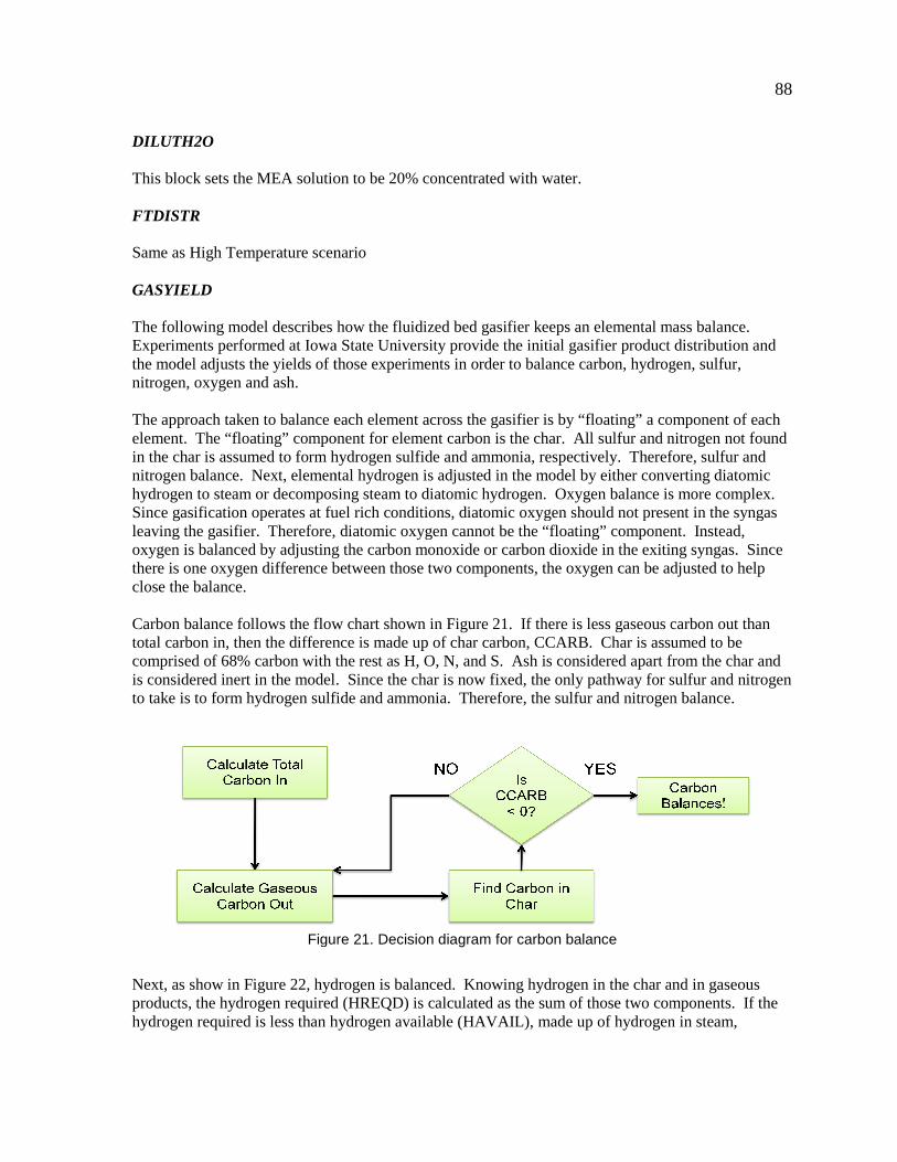
DILUTH2O This block sets the MEA solution to be 20% concentrated with water. FTDISTR Same as High Temperature scenario GASYIELD The following model describes how the fluidized bed gasifier keeps an elemental mass balance. Experiments performed at Iowa State University provide the initial gasifier product distribution and the model adjusts the yields of those experiments in order to balance carbon, hydrogen, sulfur, nitrogen, oxygen and ash. The approach taken to balance each element across the gasifier is by “floating” a component of each element. The “floating” component for element carbon is the char. All sulfur and nitrogen not found in the char is assumed to form hydrogen sulfide and amnitrogen balance. Next, elemental hydrogen is adjusted in the model by either converting diatomic hydrogen to steam or decomposing steam to diatomic hydrogen. Oxygen balance is more complex. Since gasification operates at fuel rich conditions, diatomic oxygen should not present in the syngas leaving the gasifier. Therefore, diatomic oxygen cannot be the “floating” component. Instead, oxygen is balanced by adjusting the carbon monoxide or carbon dioxide in thethere is one oxygen difference between those two components, the oxygen can be adjusted to help close the balance. Carbon balance follows the flow chart shown in total carbon in, then the difference is made up of char carbon, CCARB. Char is assumed to be comprised of 68% carbon with the rest as H, O, N, and S. Ash is consiis considered inert in the model. Since the char is now fixed, the only pathway for sulfur and nitrogen to take is to form hydrogen sulfide and ammonia. Therefore, the sulfur and nitrogen balance.

Figure

Next, as show in Figure 22, hydrogen is balanced. Knowing hydrogen in the char and in gaseous products, the hydrogen required (HREQD) is calculated as the sum of those two components. If the hydrogen required is less than hydrogen available (HAVAIL), made up of hydrogen in steam,

This block sets the MEA solution to be 20% concentrated with water.

Same as High Temperature scenario

The following model describes how the fluidized bed gasifier keeps an elemental mass balance. Experiments performed at Iowa State University provide the initial gasifier product distribution and

ts the yields of those experiments in order to balance carbon, hydrogen, sulfur,

The approach taken to balance each element across the gasifier is by “floating” a component of each element. The “floating” component for element carbon is the char. All sulfur and nitrogen not found in the char is assumed to form hydrogen sulfide and ammonia, respectively. Therefore, sulfur and nitrogen balance. Next, elemental hydrogen is adjusted in the model by either converting diatomic hydrogen to steam or decomposing steam to diatomic hydrogen. Oxygen balance is more complex.

operates at fuel rich conditions, diatomic oxygen should not present in the syngas leaving the gasifier. Therefore, diatomic oxygen cannot be the “floating” component. Instead, oxygen is balanced by adjusting the carbon monoxide or carbon dioxide in the exiting syngas. Since there is one oxygen difference between those two components, the oxygen can be adjusted to help

Carbon balance follows the flow chart shown in Figure 21. If there is less gaseous carbon out than total carbon in, then the difference is made up of char carbon, CCARB. Char is assumed to be comprised of 68% carbon with the rest as H, O, N, and S. Ash is considered apart from the char and is considered inert in the model. Since the char is now fixed, the only pathway for sulfur and nitrogen to take is to form hydrogen sulfide and ammonia. Therefore, the sulfur and nitrogen balance.

Figure 21. Decision diagram for carbon balance

, hydrogen is balanced. Knowing hydrogen in the char and in gaseous products, the hydrogen required (HREQD) is calculated as the sum of those two components. If the hydrogen required is less than hydrogen available (HAVAIL), made up of hydrogen in steam,

88

The following model describes how the fluidized bed gasifier keeps an elemental mass balance. Experiments performed at Iowa State University provide the initial gasifier product distribution and

ts the yields of those experiments in order to balance carbon, hydrogen, sulfur,

The approach taken to balance each element across the gasifier is by “floating” a component of each element. The “floating” component for element carbon is the char. All sulfur and nitrogen not found

monia, respectively. Therefore, sulfur and nitrogen balance. Next, elemental hydrogen is adjusted in the model by either converting diatomic hydrogen to steam or decomposing steam to diatomic hydrogen. Oxygen balance is more complex.

operates at fuel rich conditions, diatomic oxygen should not present in the syngas leaving the gasifier. Therefore, diatomic oxygen cannot be the “floating” component. Instead,

exiting syngas. Since there is one oxygen difference between those two components, the oxygen can be adjusted to help

. If there is less gaseous carbon out than total carbon in, then the difference is made up of char carbon, CCARB. Char is assumed to be

dered apart from the char and is considered inert in the model. Since the char is now fixed, the only pathway for sulfur and nitrogen to take is to form hydrogen sulfide and ammonia. Therefore, the sulfur and nitrogen balance.

, hydrogen is balanced. Knowing hydrogen in the char and in gaseous products, the hydrogen required (HREQD) is calculated as the sum of those two components. If the hydrogen required is less than hydrogen available (HAVAIL), made up of hydrogen in steam,

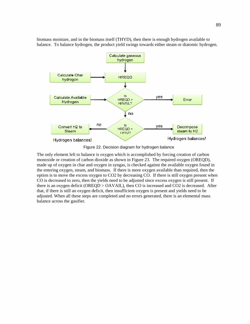
biomass moisture, and in the biomass itself (THYD), then there is enough hydrogen available to balance. To balance hydrogen, the product yield swings towards either steam or diatomic hydrogen.

Figure

The only element left to balance is oxygen which is accomplished by forcing creation of carbon monoxide or creation of carbon dioxide as shown in made up of oxygen in char and oxygen in syngas, is checked against the available oxygen found in the entering oxygen, steam, and biomass. If there is more oxygen available than required, then the option is to move the excess oxygen to CO2 by decreasing CO. If there is still oxygen present when CO is decreased to zero, then the yields need to be adjusted since excess oxygen is still present. If there is an oxygen deficit (OREQD > OAVAIL), then CO is increased and CO2 isthat, if there is still an oxygen deficit, then insufficient oxygen is present and yields need to be adjusted. When all these steps are completed and no errors generated, there is an elemental mass balance across the gasifier.

biomass moisture, and in the biomass itself (THYD), then there is enough hydrogen available to balance. To balance hydrogen, the product yield swings towards either steam or diatomic hydrogen.

Figure 22. Decision diagram for hydrogen balance

The only element left to balance is oxygen which is accomplished by forcing creation of carbon monoxide or creation of carbon dioxide as shown in Figure 23. The required oxygen (OREQD), made up of oxygen in char and oxygen in syngas, is checked against the available oxygen found in the entering oxygen, steam, and biomass. If there is more oxygen available than required, then the

xcess oxygen to CO2 by decreasing CO. If there is still oxygen present when CO is decreased to zero, then the yields need to be adjusted since excess oxygen is still present. If there is an oxygen deficit (OREQD > OAVAIL), then CO is increased and CO2 is decreased. After that, if there is still an oxygen deficit, then insufficient oxygen is present and yields need to be

all these steps are completed and no errors generated, there is an elemental mass

89

biomass moisture, and in the biomass itself (THYD), then there is enough hydrogen available to balance. To balance hydrogen, the product yield swings towards either steam or diatomic hydrogen.

The only element left to balance is oxygen which is accomplished by forcing creation of carbon . The required oxygen (OREQD),

made up of oxygen in char and oxygen in syngas, is checked against the available oxygen found in the entering oxygen, steam, and biomass. If there is more oxygen available than required, then the

xcess oxygen to CO2 by decreasing CO. If there is still oxygen present when CO is decreased to zero, then the yields need to be adjusted since excess oxygen is still present. If

decreased. After that, if there is still an oxygen deficit, then insufficient oxygen is present and yields need to be

all these steps are completed and no errors generated, there is an elemental mass

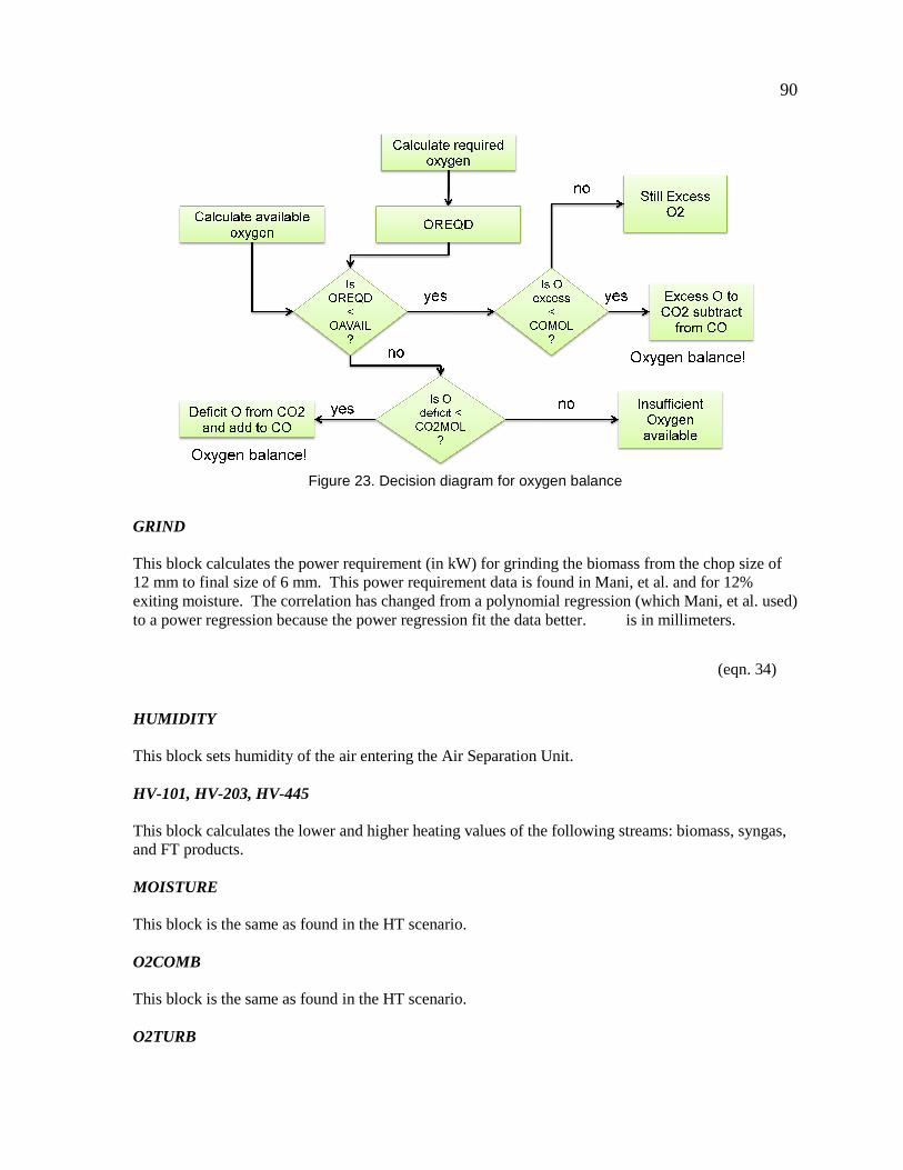
Figur

GRIND This block calculates the power requirement (in kW) for grinding the biomass from the chop size of 12 mm to final size of 6 mm. This power requirement data is found in Mani, et al.exiting moisture. The correlation has changed from a polynomial regression (which Mani, et al. used) to a power regression because the power regression fit the data better.

HUMIDITY This block sets humidity of the air entering the Air Separation Unit. HV-101, HV-203, HV-445 This block calculates the lower and higher heating values of the following streams: biomass, syngas, and FT products. MOISTURE This block is the same as found in the HT scenario. O2COMB This block is the same as found in the HT scenario. O2TURB

Figure 23. Decision diagram for oxygen balance

This block calculates the power requirement (in kW) for grinding the biomass from the chop size of 12 mm to final size of 6 mm. This power requirement data is found in Mani, et al. and for 12% exiting moisture. The correlation has changed from a polynomial regression (which Mani, et al. used) to a power regression because the power regression fit the data better. is in millimeters.

This block sets humidity of the air entering the Air Separation Unit.

This block calculates the lower and higher heating values of the following streams: biomass, syngas,

block is the same as found in the HT scenario.

This block is the same as found in the HT scenario.

90

This block calculates the power requirement (in kW) for grinding the biomass from the chop size of and for 12%

exiting moisture. The correlation has changed from a polynomial regression (which Mani, et al. used) is in millimeters.

(eqn. 34)

This block calculates the lower and higher heating values of the following streams: biomass, syngas,

91

This block is the same as found in the HT scenario. OXYSET This block sets the entering oxidizing agents, oxygen and steam, into the gasifier. A linear correlation with temperature, �;6< (in Fahrenheit), adapted from Bain for oxygen is used because as oxygen increases in the gasifier the temperature increases. Mass flow of oxygen, �̂ �,;6< , is in percentage of dry feedstock.

�̂ �,;6< � ��11.567 � 0.02375 · �;6<�/100 · �̂u7\96<< (eqn. 35)

The steam feed rate is set at 0.66 lb steam per lb oxygen.

�̂<4,69,;6< � 0.66 · �̂ �,;6< (eqn. 36)

Since 95% purity oxygen is produced in the Air Separation Unit, argon mass flow is set at 5% of molar oxygen flow.

�̂65;\+ � 0.05 · `�̂ �,;6<@J �

a / @Jd5 (eqn. 1)

C.4 Aspen Plus™ Design Specifications

C.4.1 High Temperature Scenario

DS-1 The exiting temperature of air in the heat exchanger used to pre-cool the air entering the cryogenic distillation column is varied until a net duty of zero is observed. FSSPL02 This design specification varies the fraction of unconverted syngas that is piped to area 200 for the combustion of syngas. The syngas, in turn, provides the heat required to dry the biomass. H2SPLIT This design spec calculates the required hydrogen that needs to be reserved by the PSA unit for use in Area 500: Hydrocracking. A typical yield from hydrocracking is shown in the table below. Since the FT products are be hydrogen deficient relative to the final blend, then make-up hydrogen is required. The syngas purge amount going to the pressure swing adsorption (PSA) unit is varied so that the calculated delivered hydrogen matches the required hydrogen to Area 500. Without showing the detailed calculations, the basic steps are first calculating the carbon and hydrogen content in the FT product stream. The carbon mass flow is the same as that of the final blend stream flow. Using the blend fractions in Table 38, the amount of hydrogen is calculated in the final blend and the difference

92

in hydrogen is determined. The difference is multiplied by 1.1 to obtain the delivered hydrogen mass flow rate to hydrocracking area.

Table 38. Hydroprocessing product blend

Component Mass Fraction Fuel Gas (methane) 0.034 LPG (propane) 0.088 Gasoline (n-octane) 0.261 Diesel (n-hexadecane) 0.617

O2-101, O2-203, O2-445 These design specifications vary the amount of oxygen inlet to the Heating Value blocks (HV-101, HV-203, HV-445) so as to be stoichiometric in the combustion of the duplicate stream. O2-SULF This design specification varies the amount of oxygen into the LO-CAT oxidizer unit to fully oxidize the H2S into solid sulfur. SGSTEMP The temperature of operation in the sour water-gas-shift reactor is varied until the exiting equilibrium molar ratio of H2/CO is just above the optimal FT ratio (2.1). A small amount of hydrogen is captured in the PSA unit bringing that ratio down to the optimum for FT synthesis.

C.4.2 Low Temperature scenario

DS-1 This design specification is the same as HT scenario. H2SPLIT This design specification is the same as HT scenario. O2-101, O2-203, O2-445 These design specifications are the same as in the HT scenario. O2-SULF This design specification is the same as HT scenario. STMRECOV Heat can be recovered from the combustion of syngas and char. This specification varies the steam flow rate (stream 280) to bring the combustion flue gas (stream 252) down to 200 C via heat exchanging.

93

WGSTEMP The temperature of operation in the water-gas-shift reactor is varied until the exiting equilibrium molar ratio of H2/CO is just above the optimal FT ratio (2.1). A small amount of hydrogen is captured in the PSA unit bringing that ratio down to the optimum for FT synthesis.

94

C.5 Detailed Calculations

ASPEN Model Calculations and Notes

Outline Defining Units

Plant Input Plant Output

Carbon Efficiency to Fuels

Energy Content

FT Reaction Conversion Solver

Equipment Sizing

Dryer

Lock hoppers

Slag/Char Collection

PSA Unit

Fuel Storage

LT Gasifier Cost

FT Reactor Cost

Acid Gas Removal Area Cost A500 Hydroprocessing Area Cost

Reactors and Catalysts

Natural Gas Utility Usage

MJ 106J:= MMcf 10

6ft

3:=

kPa 103

Pa⋅:= Cp 100poise:=

ρwater 1000kg

m3

:=MW H2O 18.02

gm

mol:=

kmol 1000mol:= MMBTU 106BTU:=

lbmolkmol

2.2:=

bbl 42gal:=

ρgas 737.22kg

m3

:= 100kg

m3

6.243lb

ft3

=

ρdiesel 840kg

m3

:= therm 100000BTU:=

MMgal 106gal:= dekatherm 10therm:=

kJ 1000J:= Pref 1atm≡

Tref 298K≡bpsd

42gal

day:=

PJ 1015

J:= GJ 109J:=

HHVstover 7.588 103

×BTU

lb=

HHVstover 17.65MJ

kg:=

95

Plant Input

Biomass

Elemental Composition

Carbon

Oxygen

Hydrogen

Sulfur

Nitrogen

Ash

Elemental Mass Flow

mdot_biomass 2000tonne

day:= Availability 310day:= Load 7446hr:=

FracC_biomass 0.4728≡ MW C 12.01gm

mol:=

FracO_biomass 0.4063≡ MW O 16.gm

mol:=

FracH_biomass 0.0506≡ MW H 1.01gm

mol:=

FracS_biomass 0.0022≡ MW S 32.07gm

mol:=

FracN_biomass 0.008≡ MW N 14.01gm

mol:=

FracA_biomass 0.0600≡

mdot_C_in mdot_biomassFracC_biomass⋅:= mdot_C_in 945.6tonne

day=

mdot_O_in mdot_biomassFracO_biomass⋅:= mdot_O_in 812.6tonne

day=

mdot_H_in mdot_biomassFracH_biomass⋅:= mdot_H_in 101.2tonne

day=

mdot_S_in mdot_biomassFracS_biomass⋅:= mdot_S_in 4.4tonne

day=

mdot_N_in mdot_biomassFracN_biomass⋅:= mdot_N_in 16tonne

day=

mdot_A_in mdot_biomassFracA_biomass⋅:= mdot_A_in 120tonne

day=

96

Elemental Mole Flow

Biomass Moisture

Source: Kaliyan and Morey, 2005 for 0.66-0.8 mm sized particles

ndot_C_in

mdot_C_in

MW C:= ndot_C_in 911.278

mol

s=

ndot_O_in

mdot_O_in

MW O:= ndot_O_in 587.818

mol

s=

ndot_H_in

mdot_H_in

MW H:= ndot_H_in 1160

mol

s=

ndot_S_in

mdot_S_in

MW S:= ndot_S_in 1.588

mol

s=

ndot_N_in

mdot_N_in

MW N:= ndot_N_in 13.218

mol

s=

moistin 0.25:= moistdried 0.10:=

mdot_moist_in

moistin mdot_biomass⋅

1 moistin−:= mdot_moist_in 666.667

tonne

day=

mdot_moist_dried

moistdried mdot_biomass⋅

1 moistdried−:= mdot_moist_dried 222.222

tonne

day=

ρbulk_stover 100kg

m3

:=

97

HT Gasifier Steam/Oxygen addition Source: Probstein and Hicks, 2006

Stoichiometric/thermoneutral requirement for synthesis gas according to following equation: 1.34C + 0.34 O2 + H2O --> 0.34CO2 + CO + H2 Oxygen to Carbon: 0.25 Steam to Carbon : 0.75

Steam addition ratio is then three times that of Oxygen minus the moisture in the biomass

mdot_O2_in 0.35 mdot_biomass⋅:= mdot_O2_in 700tonne

day=

ndot_O2_in

mdot_O2_in

2 MWO⋅:= ndot_O2_in 253.183

mol

s=

RatioO2_to_C

ndot_O2_in

ndot_C_in:= RatioO2_to_C 0.278=

ndot_H2O_in 3 RatioO2_to_C⋅ ndot_C_in⋅mdot_moist_dried

MW H2O−:=

mdot_H2O_in ndot_H2O_inMW H2O⋅:=

ndot_H2O_in 616.817mol

s=

mdot_H2O_in 960tonne

day=

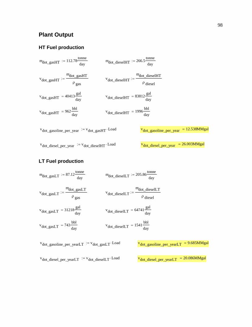
98

Plant Output

HT Fuel production

LT Fuel production

mdot_gasHT 112.78tonne

day:= mdot_dieselHT 266.5

tonne

day:=

vdot_gasHT

mdot_gasHT

ρgas:= vdot_dieselHT

mdot_dieselHT

ρdiesel:=

vdot_gasHT 40413gal

day= vdot_dieselHT 83812

gal

day=

vdot_gasHT 962bbl

day= vdot_dieselHT 1996

bbl

day=

vdot_gasoline_per_year vdot_gasHTLoad⋅:=

vdot_diesel_per_year vdot_dieselHTLoad⋅:=

mdot_gasLT 87.12tonne

day:= mdot_dieselLT 205.86

tonne

day:=

vdot_gasLT

mdot_gasLT

ρgas:= vdot_dieselLT

mdot_dieselLT

ρdiesel:=

vdot_gasLT 31218gal

day= vdot_dieselLT 64741

gal

day=

vdot_gasLT 743bbl

day= vdot_dieselLT 1541

bbl

day=

vdot_gasoline_per_yearLT vdot_gasLTLoad⋅:= vdot_gasoline_per_yearLT 9.685MMgal=

vdot_diesel_per_yearLT vdot_dieselLT Load⋅:= vdot_diesel_per_yearLT 20.086MMgal=

vdot_gasoline_per_year 12.538MMgal=

vdot_diesel_per_year 26.003MMgal=

99

Carbon Efficiency to Fuels

HT scenario

Gasoline Carbon

Diesel Carbon

mdot_gasHT 112.78tonne

day=

mdot_C_gasHT FracC_gasolinemdot_gasHT⋅:= mdot_C_gasHT 94.835tonne

day=

mdot_dieselHT 266.5tonne

day=

FracC_diesel16 12.01⋅

16 12.01⋅ 34 1.01⋅+:= FracC_diesel 0.848=

mdot_C_dieselHT FracC_dieselmdot_dieselHT⋅:= mdot_C_dieselHT 226.096tonne

day=

mdot_C_outHT mdot_C_gasHT mdot_C_dieselHT+:=

mdot_C_outHT 320.931tonne

day= C_effHT

mdot_C_outHT

mdot_C_in:=

FracC_gasoline8 12.01⋅

8 12.01⋅ 181.01⋅+:= FracC_gasoline 0.841=

C_effHT 0.339=

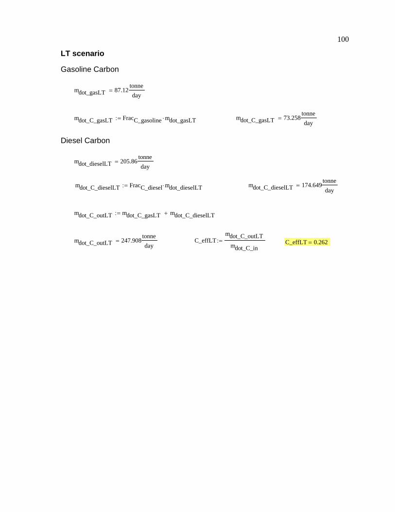
100

LT scenario

Gasoline Carbon

Diesel Carbon

mdot_gasLT 87.12tonne

day=

mdot_C_gasLT FracC_gasolinemdot_gasLT⋅:= mdot_C_gasLT 73.258tonne

day=

mdot_dieselLT 205.86tonne

day=

mdot_C_dieselLT FracC_dieselmdot_dieselLT⋅:= mdot_C_dieselLT 174.649tonne

day=

mdot_C_outLT mdot_C_gasLT mdot_C_dieselLT+:=

mdot_C_outLT 247.908tonne

day= C_effLT

mdot_C_outLT

mdot_C_in:= C_effLT 0.262=

101

Energy Content This section aquires the energy content (on a LHV basis) from the Aspen data and converts to megawatts for use in developing an energy balance

Biomass

Fuel

Char/Tar

Raw Syngas

Energy loss across the gasifier Energy lost across the gasifier is calculated as difference in energy in the biomass and energy in the raw syngas and char (only in LT scenario)

Ebiomass 1400313MJ

hr:= Ebiomass 388.976MW=

EfuelHT 695598MJ

hr:= EfuelHT 193.222MW=

EfuelLT 539292MJ

hr:= EfuelLT 149.803MW=

Echar_LT 87792MJ

hr:= Echar_LT 24.387MW=

Etar_LT 16980MJ

hr:= Etar_LT 4.717MW=

Erawsyngas_HT 1230712MJ

hr:= Erawsyngas_HT 341.864MW=

Erawsyngas_LT 964054MJ

hr:= Erawsyngas_LT 267.793MW=

Egasifierloss_HT Ebiomass Erawsyngas_HT−:=

Egasifierloss_LT Ebiomass Erawsyngas_LT− Echar_LT−:=

Egasifierloss_HT 47.111MW=

Egasifierloss_LT 96.796MW=

102

Unconverted Syngas used in A600 Power Generation

Fuel Gas from A500 used in A600 Power Generation

Fischer-Tropsch product

Electricity Generated

Net Electricity (exported)

Power Generation loss

The loss is the difference between electric generation out and the gas energy in

EsyngasA600_HT 129332MJ

hr:= EsyngasA600_HT 35.926MW=

EsyngasA600_LT 109708MJ

hr:= EsyngasA600_LT 30.474MW=

Efuelgas_HT 104114MJ

hr:= Efuelgas_HT 28.921MW=

Efuelgas_LT 80718MJ

hr:= Efuelgas_LT 22.422MW=

EFTliquids_HT 782894MJ

hr:= EFTliquids_HT 217.471MW=

EFTliquids_LT 606801MJ

hr:= EFTliquids_LT 168.556MW=

EelecgenOUT_HT 48.55MW:= EelecgenOUT_LT 40.73MW:=

Eelecnet_HT 13.8MW:= Eelecnet_LT 16.3MW:=

EA600losses_HT EsyngasA600_HT Efuelgas_HT+ EelecgenOUT_HT−:=

EA600losses_HT 16.296MW=

EA600losses_LT EsyngasA600_LT Efuelgas_LT+ EelecgenOUT_LT−:=

EA600losses_LT 12.166MW=

103

Loss across FT reactor

Unconverted Syngas used for biomass drying

Only in HT scenario

EFTreactorlosses_HT 226737MJ

hr:= EFTreactorlosses_HT 62.983MW=

EFTreactorlosses_LT 175128MJ

hr:= EFTreactorlosses_LT 48.647MW=

Ebiomass_drying_HT 24663MJ

hr:= Ebiomass_drying_HT 6.851MW=

104

Fischer-Tropsch Reaction Conversion Solver

This section solves for the reaction fractional conversion for each reaction in the Fischer-Tropsch reactor. A set of equations is developed and solved. The resulting ε values (ε1 - ε30) are used directly in the Aspen Plus conversion reactor block. The reactions in the reactor block are defined as molar extent.

Depending on the alpha chain growth probability, the reactor forms different product composition.

Step 1: choose the expected alpha chain growth value

Step 2: using the αFT chain growth, the mole fraction of each hydrocarbon in the FT product is calculated.

All hydrocarbons greater than C20 make up the balance and modeled using C30.

αFT 0.9:=

M1 αFT1 1−

1 αFT−( )⋅:= M1 0.1= M11 αFT11 1−

1 αFT−( )⋅:=

M2 αFT2 1−

1 αFT−( )⋅:= M2 0.09= M12 αFT12 1−

1 αFT−( )⋅:=

M3 αFT3 1−

1 αFT−( )⋅:= M3 0.081= M13 αFT13 1−

1 αFT−( )⋅:=

M4 αFT4 1−

1 αFT−( )⋅:= M4 0.073= M14 αFT14 1−

1 αFT−( )⋅:=

M5 αFT5 1−

1 αFT−( )⋅:= M5 0.066= M15 αFT15 1−

1 αFT−( )⋅:=

M6 αFT6 1−

1 αFT−( )⋅:= M6 0.059= M16 αFT16 1−

1 αFT−( )⋅:=

M7 αFT7 1−

1 αFT−( )⋅:= M7 0.053= M17 αFT17 1−

1 αFT−( )⋅:=

M8 αFT8 1−

1 αFT−( )⋅:= M8 0.048= M18 αFT18 1−

1 αFT−( )⋅:=

M9 αFT9 1−

1 αFT−( )⋅:= M9 0.043= M19 αFT19 1−

1 αFT−( )⋅:=

M10 αFT10 1−

1 αFT−( )⋅:= M10 0.039= M20 αFT20 1−

1 αFT−( )⋅:=

M30 1 M1 M2+ M3+ M4+ M5+ M6+ M7+ M8+ M9+ M10+M11 M12+ M13+ M14+ M15+ M16+ M17+ M18+ M19+ M20++

...

−:=

M30 0.122=

M11 0.035=

M12 0.031=

M13 0.028=

M14 0.025=

M15 0.023=

M16 0.021=

M17 0.019=

M18 0.017=

M19 0.015=

M20 0.014=

105

Step 3: Setup a series of equations to solve along with guess values (required for Mathcad)

For a nominal 1000 moles of CO input, the expected CO output is 600 moles since 40% is converted.

<----------------- 40% conversion of CO

<----- This value to be varied until COconv is equal to desired.

A nominal 400 moles of CO are converted in the FT reactor. The sum of the exiting amount of moles in the FT product distribution will not be 400, since moles are not conserved. Mass is conserved, however. Therefore, the variable "D" represents a factor that adjusts all the conversions (ε1, ε2, etc.). The resulting value of D is 0.1 meaning that 40 moles of FT products exit the reactor.

Known COout 600:= COin 1000:=

Guess ε1 20:= ε2 20:= ε3 20:= ε4 20:= ε5 20:=

ε6 20:= ε7 20:= ε8 20:= ε9 20:= ε10 20:=

ε11 20:= ε12 20:= ε13 20:= ε14 20:= ε15 20:=

ε16 20:= ε17 20:= ε18 20:= ε19 20:= ε20 20:=

ε30 20:= D 0.1:=

Given

D ε11

2ε2+

1

3ε3+

1

4ε4+

1

5ε5+

1

6ε6+

1

7ε7+

1

8ε8+

1

9ε9+

1

10ε10+

1

11ε11+

1

12ε12+

1

13ε13

1

14ε14+

1

15ε15+

1

16ε16+

1

17ε17+

1

18ε18+

1

19ε19+

1

20ε20+

1

30ε30++

...

M1ε1

DM2

1

2ε2

DM3

1

3ε3

DM4

1

4ε4

DM5

1

5ε5

DM6

1

6ε6

D

M7

1

7ε7

DM8

1

8ε8

DM9

1

9ε9

DM10

1

10ε10

DM11

1

11ε11

DM12

1

12ε12

D

M13

1

13ε13

DM14

1

14ε14

DM15

1

15ε15

DM16

1

16ε16

DM17

1

17ε17

DM18

1

18ε18

D

M19

1

19ε19

DM20

1

20ε20

DM30

1

30ε30

D

Solve Findε1 ε2, ε3, ε4, ε5, ε6, ε7, ε8, ε9, ε10, ε11, ε12, ε13, ε14, ε15, ε16, ε17, ε18, ε19, ε20, ε30,( ):=

Solve0

0

1

0.01

0.018

=

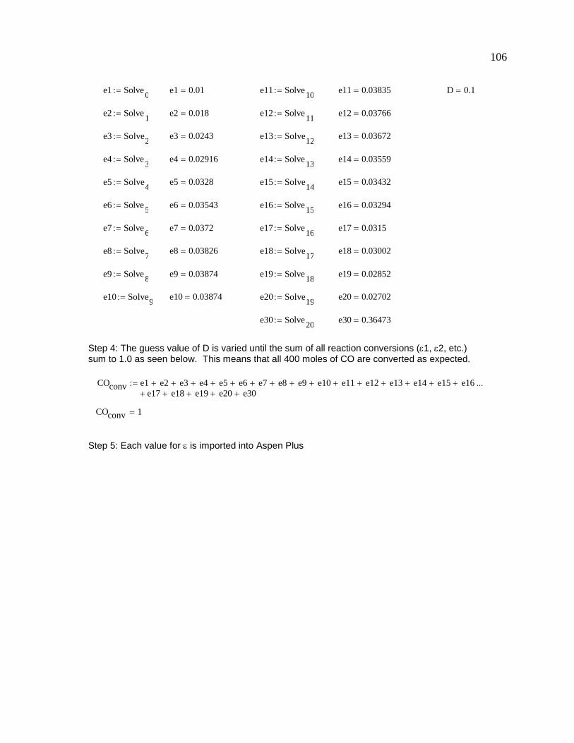
106

Step 4: The guess value of D is varied until the sum of all reaction conversions (ε1, ε2, etc.) sum to 1.0 as seen below. This means that all 400 moles of CO are converted as expected.

Step 5: Each value for ε is imported into Aspen Plus

e1 Solve0

:= e1 0.01= e11 Solve10

:= e11 0.03835= D 0.1=

e2 Solve1

:= e2 0.018= e12 Solve11

:= e12 0.03766=

e3 Solve2

:= e3 0.0243= e13 Solve12

:= e13 0.03672=

e4 Solve3

:= e4 0.02916= e14 Solve13

:= e14 0.03559=

e5 Solve4

:= e5 0.0328= e15 Solve14

:= e15 0.03432=

e6 Solve5

:= e6 0.03543= e16 Solve15

:= e16 0.03294=

e7 Solve6

:= e7 0.0372= e17 Solve16

:= e17 0.0315=

e8 Solve7

:= e8 0.03826= e18 Solve17

:= e18 0.03002=

e9 Solve8

:= e9 0.03874= e19 Solve18

:= e19 0.02852=

e10 Solve9

:= e10 0.03874= e20 Solve19

:= e20 0.02702=

e30 Solve20

:= e30 0.36473=

COconv e1 e2+ e3+ e4+ e5+ e6+ e7+ e8+ e9+ e10+ e11+ e12+ e13+ e14+ e15+ e16+e17 e18+ e19+ e20+ e30++

...:=

COconv 1=

107

Equipment Sizing

Rotary Dryer Source: Process Engineering Economics by James Couper, 2003

Typical rpm of rotary dryers

Typical product of equals 15-25. Assume value of 25 for larger end

Typical residence times are 5-90 minutes and holdup of solids is 7-8%. Assume 5 minutes and 8%.

Typical exit gas temperature is 10-20°C above the e ntering solids.

Feed rate into plant is 2000 ton/day with bulk density of stover equal to 100kg/m^3. Water density is accounted for as well.

Volume of solids in dryer

Volume of solids and steam

Length of theoretical dryer

Surface area of theoretical dryer

Max surface area as reported by Aspen Icarus is 185 m2, therefore approximately 10 dryers are required.

Feed throughput in each dryer (used for Icarus input)

rpmdryer 4:=

rpm diameter feet( )⋅

Ddryer25ft

rpmdryer:= Ddryer 6.25ft=

tres 5min:= holdup 0.08:=

mdot_feed 2000tonne

day:= mdot_moist_in 666.667

tonne

day=

ρbulk_stover 100kg

m3

= ρwater 1000kg

m3

=

Vsolids

mdot_feed

ρbulk_stover

mdot_moist_in

ρwater+

tres⋅:=

Vdryer_total

Vsolids

holdup:=

lengthdryer

Vdryer_total

Ddryer2 π

4⋅

:=

Asurf_dryer lengthdryer π⋅ Ddryer⋅:=

mdot_feed mdot_moist_in+

1024495.8

lb

hr=

Vsolids 71.759m3

=

Vdryer_total 896.991m3

=

lengthdryer 314.708m=

Asurf_dryer 1883.4m2

=

108

Lock hopper System

Source: CE IGCC Repowering Project Bins and Lockhoppers, Combustion Eng. 1993

note: this report's feedstock is coal

Assumptions from report -A receiving bin is situated before the lockhopper with a 40 minute residence time -design pressure is for 50 psia. -Cycle time for lockhopper system is designed for 10 minutes resulting in approximately 50,000 cycles per year -Storage volume for lockhopper and feed bin is assumed to be 10 minutes -Approximate lockhopper and feed bin vessel thickness is 1.5 inches and design pressure is for 450 psia -Volume is theoretical + 33%

Residence Time

biomass receiving bin

biomass lockhopper

biomass feed bin

Density of feed

HT Scenario Lockhopper system (1 train)

Volume of biomass receiving bin

Volume of biomass lockhopper

Volume of biomass feed bin

tres_rbin 40min:= εvoid 25%:=

tres_lock 10min:=

tres_fbin 10min:=

mdot_feed_lock mdot_feed mdot_moist_dried+:=

mdot_feed_lock 2222tonne

day=

ρstover_10%moist

ρbulk_stover 2000⋅ ρwater222⋅+

2222:=

ρstover_10%moist 189.919kg

m3

=

Vr_bin

tres_rbinmdot_feed_lock⋅

ρstover_10%moist

1

1 εvoid−⋅:=

Vlock

tres_lockmdot_feed_lock⋅

ρstover_10%moist

1

1 εvoid−⋅:=

Vf_bin

tres_fbinmdot_feed_lock⋅

ρstover_10%moist

1

1 εvoid−⋅:=

Vr_bin 433m3

=

Vlock 108m3

=

Vf_bin 108m3

=

109

Low Temperature Lockhopper System (7 trains)

Volume of biomass receiving bin

Volume of biomass lockhopper

Volume of biomass feed bin

Source: Combustion Engineering 1993

Vr_binLT

Vr_bin

7:=

VlockLT

Vlock

7:=

Vf_binLT

Vf_bin

7:=

Vr_binLT 61.909m3

=

VlockLT 15.477m3

=

Vf_binLT 15.477m3

=

110

Lockhopper Power Consumption

Source: Techno-Economic Analysis of Hydrogen Production by Gasification of Biomass by Lau et al. [2002]

Specific Power of lockhopper, kW/tonne/day

Biomass inlet to gasifier

SPlock 0.082kW

tonne

day

:=

mdot_gasifier mdot_biomass mdot_moist_dried+:=

Powerlock SPlock mdot_gasifier⋅:= Powerlock 182.222kW=

111

Fly Ash Collection Storage Tank (assume 7 days storage)

(assumed)

Slag Separation drum (5 minute residence time, 20% volume)

Slag collection Storage tank (7 days storage)

Char collection storage bin (1-day residence time, 80% volume)

Note: the resulting volumes are used to assist in costing using Aspen Icarus

assume 20% voidage

ρash 700kg

m3

:= mdot_ash 5.88tonne

day:=

Vtank

mdot_ash

ρash7⋅ day:= Vtank 58.8m

3= Vtank 2.077 10

3× ft

3=

ρslag 2700kg

m3

:= mdot_slag 114tonne

day:= εvoid_slag 0.8:=

Vdrum

mdot_slag

ρslag5⋅ min

1

1 εvoid_slag−⋅:= Vdrum 0.733m

3=

Vslag_storage

mdot_slag

ρslag7⋅ day:=

ρchar 2700kg

m3

:= mdot_char 214tonne

day:=

Vchardrum

mdot_char

ρchar1⋅ day

1

1 εvoid_char−⋅:=

Vslag_storage 295.6m3

=

εvoid_char 0.2:=

Vchardrum 99.074m3

=

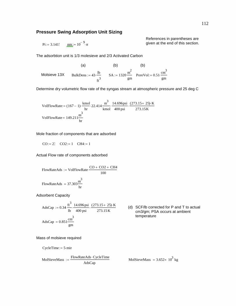
112

Pressure Swing Adsorption Unit Sizing

The adsorbtion unit is 1/3 molesieve and 2/3 Activated Carbon

(a) (b) (b)

Molsieve 13X

Determine dry volumetric flow rate of the syngas stream at atmospheric pressure and 25 deg C

Mole fraction of components that are adsorbed

Actual Flow rate of components adsorbed

Adsorbent Capacity

(d) SCF/lb corrected for P and T to actual cm3/gm; PSA occurs at ambient temperature

Mass of molsieve required

References in parentheses are given at the end of this section. Pi 3.1415:= nm 10

9−m⋅:=

BulkDens 43lb

ft3

⋅:= SA 1320m

2

gm⋅:= PoreVol 0.51

cm3

gm⋅:=

VolFlowRate 167 1−( )kmol

hr⋅ 22.414⋅

m3

kmol⋅

14.696psi⋅

400 psi⋅⋅

273.15 25+( ) K⋅

273.15K⋅⋅:=

VolFlowRate 149.211m

3

hr=

CO 23:= CO2 1:= CH4 1:=

FlowRateAds VolFlowRateCO CO2+ CH4+

100⋅:=

FlowRateAds 37.303m

3

hr=

AdsCap 0.34ft

3

lb⋅

14.696psi⋅

400 psi⋅⋅

273.15 25+( ) K⋅

273.15 K⋅⋅:=

AdsCap 0.851cm

3

gm=

CycleTime 5min⋅:=

MolSieveMassFlowRateAds CycleTime⋅

AdsCap:= MolSieveMass 3.652 10

3× kg=

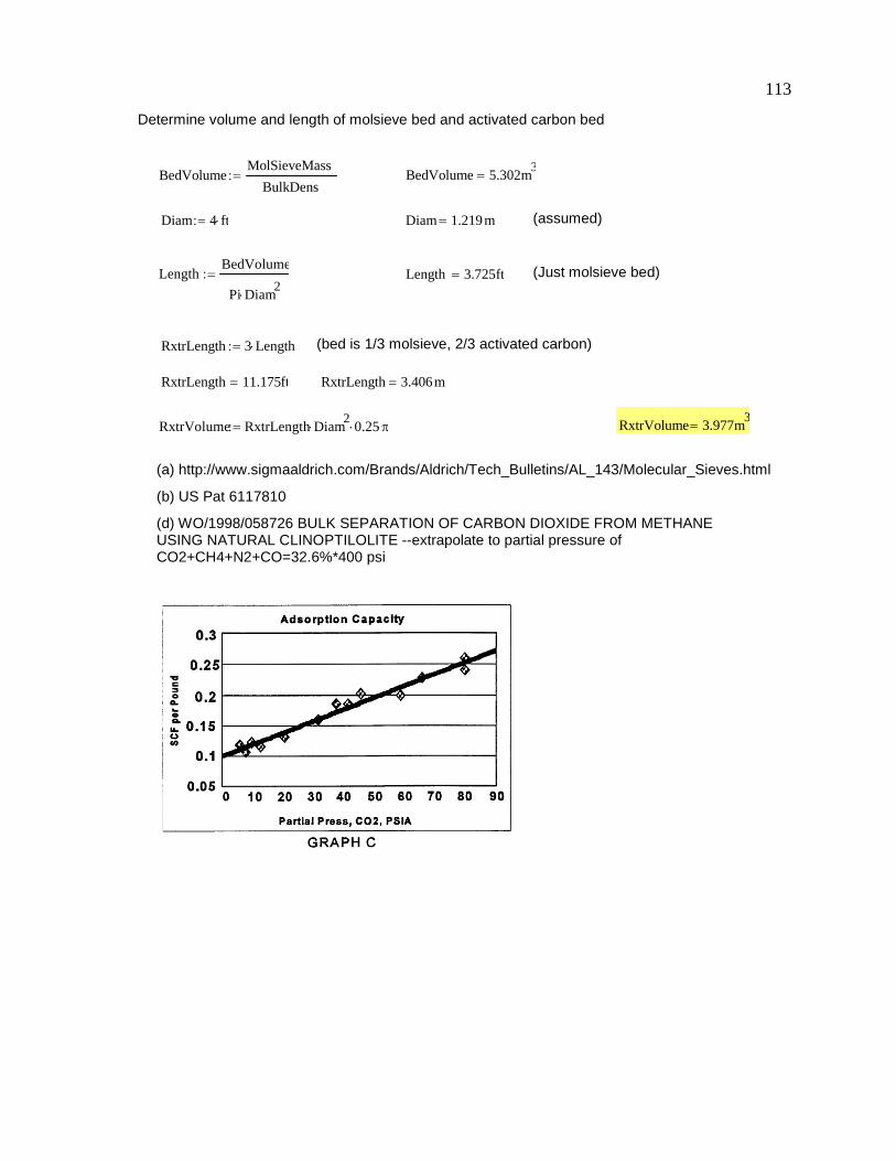
113

Determine volume and length of molsieve bed and activated carbon bed

(assumed)

(Just molsieve bed)

(bed is 1/3 molsieve, 2/3 activated carbon)

(a) http://www.sigmaaldrich.com/Brands/Aldrich/Tech_Bulletins/AL_143/Molecular_Sieves.html

(b) US Pat 6117810

(d) WO/1998/058726 BULK SEPARATION OF CARBON DIOXIDE FROM METHANE USING NATURAL CLINOPTILOLITE --extrapolate to partial pressure of CO2+CH4+N2+CO=32.6%*400 psi

BedVolumeMolSieveMass

BulkDens:= BedVolume 5.302m

3=

Diam 4ft⋅:= Diam 1.219m=

LengthBedVolume

Pi Diam2

⋅

:= Length 3.725ft=

RxtrLength 3 Length⋅:=

RxtrLength 11.175ft= RxtrLength 3.406m=

RxtrVolume RxtrLength Diam2

⋅ 0.25⋅ π⋅:= RxtrVolume 3.977m3

=

114

HT Scenario Fuel Storage

Gasoline Storage Tank (30 days storage)

Diesel Storage Tank (30 days storage)

Note: the resulting volumes are used to assist in costing using Aspen Icarus

mdot_gasHT 112.78tonne

day=

vdot_gasHT 4.041 104

×gal

day=

Vgas_tankHT vdot_gasHT 30⋅ day:=

Vgas_tankHT 4589m3

=

mdot_dieselHT 266.5tonne

day=

vdot_dieselHT 8.381 104

×gal

day=

Vdiesel_tankHT vdot_dieselHT30⋅ day:=

Vdiesel_tankHT 9518m3

=

115

LT Scenario Fuel Storage

Gasoline Storage Tank (30 days storage)

Diesel Storage Tank (30 days storage)

Note: the resulting volumes are used to assist in costing using Aspen Icarus

mdot_gasLT 87.12tonne

day=

vdot_gasLT 3.122 104

×gal

day=

Vgas_tankLT vdot_gasLT30⋅ day:=

Vgas_tankLT 3545m3

=

mdot_dieselLT 205.86tonne

day=

vdot_dieselLT 6.474 104

×gal

day=

Vdiesel_tankLT vdot_dieselLT30⋅ day:=

Vdiesel_tankLT 7352m3

=

116

LT Gasifier Cost

Source: Larson et al. 2005 in 2003$

$MM

Biomass throughput of 300 tpd

The cost ($MM) of one train at 300 ton per day

$MM

Since 2205 ton /day we need 7 gasifiers but we can apply the multiple train scaling exponent

$MM

C0_gasifier 6.41 106

⋅:= S0_gasifier 41.7tonne

hr:= Smax 120

tonne

hr:=

SgasifierLT 300ton

day:= SgasifierLT 11.34

tonne

hr=

CgasifierLT C0_gasifier

SgasifierLT

tonne

hr

1

S0_gasifier

tonne

hr

⋅

f

⋅:=

CgasifierLT 2.576 106

×=

mtrain 0.9:=

CgasifierLTtrain CgasifierLT 7mtrain

⋅:= CgasifierLTtrain 1.484 107

×=

f 0.7:=

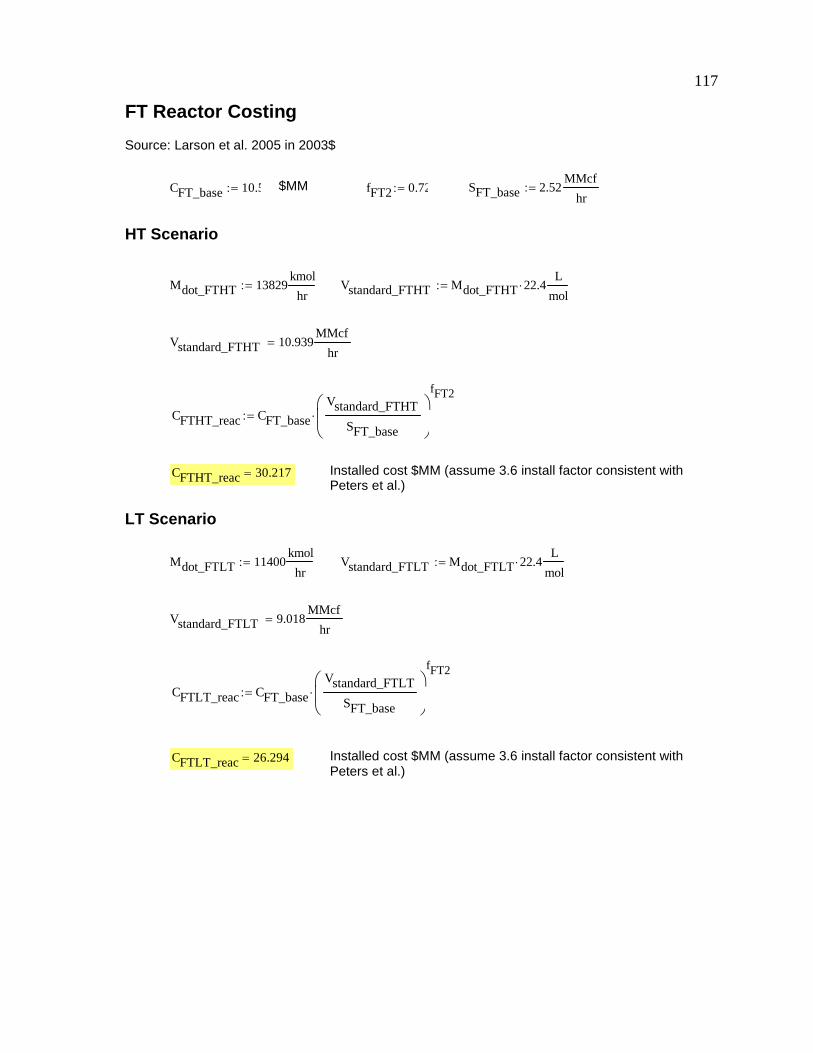
117

FT Reactor Costing

Source: Larson et al. 2005 in 2003$

$MM

HT Scenario

Installed cost $MM (assume 3.6 install factor consistent with Peters et al.)

LT Scenario

Installed cost $MM (assume 3.6 install factor consistent with Peters et al.)

CFT_base 10.5:= fFT2 0.72:= SFT_base 2.52MMcf

hr:=

Mdot_FTHT 13829kmol

hr:= Vstandard_FTHT Mdot_FTHT 22.4⋅

L

mol:=

Vstandard_FTHT 10.939MMcf

hr=

CFTHT_reac CFT_base

Vstandard_FTHT

SFT_base

fFT2

⋅:=

CFTHT_reac 30.217=

Mdot_FTLT 11400kmol

hr:= Vstandard_FTLT Mdot_FTLT 22.4⋅

L

mol:=

Vstandard_FTLT 9.018MMcf

hr=

CFTLT_reac CFT_base

Vstandard_FTLT

SFT_base

fFT2

⋅:=

CFTLT_reac 26.294=

118

Acid Gas Removal Area Cost

Source: Phillips et al. 2007 in 2005$

Calculated by adding the input syngas streams to the absorber column

HT scenario

LT scenario

SAGR_base 332910lb

hr:= fAGR 0.65:= CAGR_base 5446503:=

SAGR_HT 2965 2308+( )tonne

day⋅:= SAGR_HT 484374

lb

hr=

CAGR_HT CAGR_base

SAGR_HT

lb

hr

1

SAGR_base

lb

hr

⋅

fAGR

⋅:= CAGR_HT 6949808=

SAGR_LT 2070 2190+( )tonne

day:= SAGR_LT 391321

lb

hr=

CAGR_LT CAGR_base

SAGR_LT

lb

hr

1

SAGR_base

lb

hr

⋅

fAGR

⋅:= CAGR_LT 6049946=

119

A500 Hydroprocessing area cost

Source: Robinson et al. 2007 in 2007$

Note: "bpsd" is barrels per standard day

HT scenario

(from ASPEN model)

Power required for A500

LT Scenario

(from ASPEN model)

Power required for A500

(assumed) AreaCost04000

bpsd:= S0_HY 25000bpsd:=

C0_HY AreaCost0 S0_HY⋅:= C0_HY 100000000=

mdot_FTL_HT 428tonne

day:= ρFTL 750

kg

m3

:=

vdot_FTL_HT

mdot_FTL_HT

ρFTL:= vdot_FTL_HT 3.589 10

3× bpsd=

CHY_HT C0_HY

vdot_FTL_HT

bpsd

1

S0_HY

bpsd

⋅

fHY

⋅:= CHY_HT 2.832 107

×=

Powerper_bpsd15kW hr⋅

bpsd day⋅:=

PowerareaHT Powerper_bpsdvdot_FTL_HT⋅:= PowerareaHT 2.243MW=

mdot_FTL_LT 330.42tonne

day:=

vdot_FTL_LT

mdot_FTL_LT

ρFTL:= vdot_FTL_LT 2.771 10

3× bpsd=

CHY_LT C0_HY

vdot_FTL_LT

bpsd

1

S0_HY

bpsd

⋅

fHY

⋅:= CHY_LT 2.394 107

×=

PowerareaLT Powerper_bpsdvdot_FTL_LT⋅:= PowerareaLT 1.732MW=

fHY 0.65:=

120

Reactors and Catalysts

Fischer-Tropsch reactor and cobalt catalyst

FT reactor volume

Using gas hourly space velocity and actual volumetric flow rate, the volume of the reactor is determined

(assumed)

(from ASPEN model)

FT catalyst cost

(assumed) (assumed)

Replacement cost of cobalt catalyst

GHSVν0

V

GHSVFT 100 hr1−

⋅:=

ν rate_actHT 6.298m

3

s:=

VFTHT

νrate_actHT

GHSVFT:= VFTHT 226.728m

3= VFTHT 8.007 10

3× ft

3=

νrate_actLT 5.021m

3

s:=

VFTLT

νrate_actLT

GHSVFT:= VFTLT 180.756m

3= VFTLT 6.383 10

3× ft

3=

Cocost15

lb:= ρCo 64

lb

ft3

:=

Covol_cost Cocost ρCo⋅:= Covol_cost 9601

ft3

=

Cototal_costHT Covol_cost VFTHT⋅:= Cototal_costHT 7.687 106

×=

Cototal_costLT Covol_cost VFTLT⋅:= Cototal_costLT 6.128 106

×=

121

Water Gas Shift reactor and catalyst

Sour WGS reactor volume (HT scenario)

Using gas hourly space velocity and actual volumetric flow rate, the volume of the reactor is determined

(assumed)

(from ASPEN)

WGS reactor volume (LT scenario)

(from ASPEN)

WGS and SWGS Catalyst Cost

Replacement cost of WGS catalyst

GHSVν0

V

GHSVWGS 1000 hr1−

⋅:=

ν rate_actSWGS 2.008m

3

s:=

VSWGS

νrate_actSWGS

GHSVWGS:= VSWGS 7.229m

3= VSWGS 255.283ft

3=

ν rate_actWGS 1.834m

3

s:=

VWGS

νrate_actWGS

GHSVWGS:= VWGS 6.602m

3= VWGS 233.162ft

3=

CatCostWGS8

lb:= ρcat_WGS 56

lb

ft3

:= ρcat_WGS 897.034kg

m3

=

CatCostvol_WGS CatCostWGSρcat_WGS⋅:= CatCostvol_WGS 4481

ft3

=

TotalCatCostSWGS CatCostvol_WGS VSWGS⋅:= TotalCatCostSWGS 114367=

TotalCatCostWGS CatCostvol_WGS VWGS⋅:= TotalCatCostWGS 104456=

122

Steam Methane Reformer reactor and catalyst (LT scenario)

(assumed)

(from Aspen model)

SMR Catalyst Cost

Replacement cost of SMR catalyst

GHSVSMR 2600hr1−

:=

ν rate_actSMR 7.082m

3

s:=

VSMR

νrate_actSMR

GHSVSMR:= VSMR 9.806m

3= VSMR 346.29ft

3=

CatCostSMR4.67

lb:= ρcat_SMR 64

lb

ft3

:= ρcat_SMR 1.025 103

×kg

m3

=

CatCostvol_SMR CatCostSMR ρcat_SMR⋅:= CatCostvol_SMR 298.881

ft3

=

TotalCatCostSMR CatCostvol_SMR VSMR⋅:= TotalCatCostSMR 103499=

123

Natural Gas utility consumption

Annual natural gas requirement at 5% of yearly operating hours

Natural gas properties

HT scenario

(from Aspen model, includes power required for gas turbine air compressor)

(assumed)

Annual natural gas requirement

Average flowrate of natural gas

Price (Source: Energy Information Administration)

Costng6.4

1000ft3

:=HHVng 54

MJ

kg:= MW ng 16.04

gm

mol:= ρng 22.4

L

mol:=

Costng

ρng

MWng⋅ 286.335

1

ton=

Prequired_plantHT 32.813MW:=

Effng_to_power 0.35:=

mdot_ngHT

Prequired_plantHT

Effng_to_power

HHVng:= mdot_ngHT 1.378 10

4×

lb

hr=

MngHT mdot_ngHT Availability⋅ 0.05⋅:= MngHT 2563ton=

mdot_ng_5%HT

MngHT

8760hr:= mdot_ng_5%HT 585.14

lb

hr=

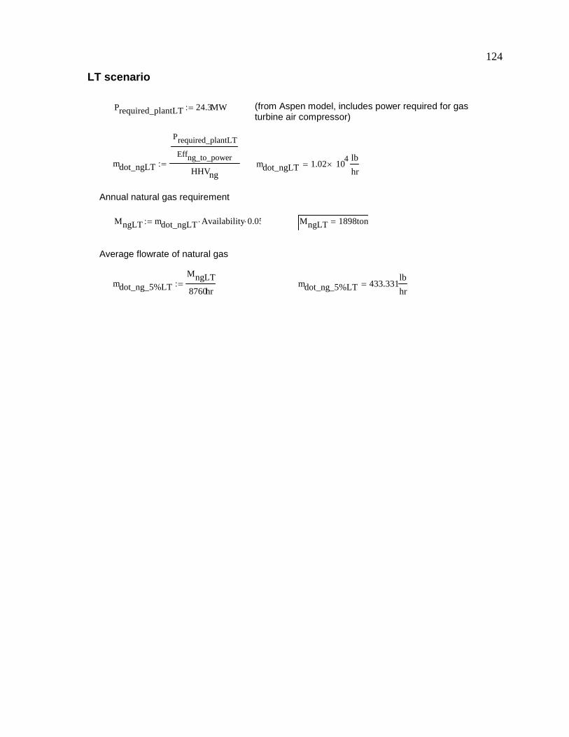
124

LT scenario

(from Aspen model, includes power required for gas turbine air compressor)

Annual natural gas requirement

Average flowrate of natural gas

Prequired_plantLT 24.3MW:=

mdot_ngLT

Prequired_plantLT

Effng_to_power

HHVng:= mdot_ngLT 1.02 10

4×

lb

hr=

MngLT mdot_ngLT Availability⋅ 0.05⋅:= MngLT 1898ton=

mdot_ng_5%LT

MngLT

8760hr:= mdot_ng_5%LT 433.331

lb

hr=

125

APPENDIX D. PROCESS FLOW DIAGRAMS

D.1 High Temperature Scenario

126

Figure 24. Overall plant area process flow diagram for HT scenario

5/22/2009Ryan Swanson HT Scenario

Overall Plant

Key

Mass Flow (tonne/day)

Temperature (°C)

Pressure (bar)

A100:

Preprocessing

A200:

Gasification

A300: Syngas

Cleaning

A400: Fuel

Synthesis

A500:

Hydroprocessing

A600: Power

Generation

A700: Air

Separation Unit

PL00BMAS

PL08BMAS PL21SGAS

PL90OX

PL34SGAS

PL50FT

PL49SGAS

PL88FLUE

PL81DIES

PL42CO2

PL89AIR PL92NTGN

PL84STM

PL81STM

PL52FLUE

PL17SLAG

PL47SGAS

PL09AIRPL43CO2

PL83SUL

PL81WAT

PL48SGASPL90HYD

25

1.01

2667

PL92WAT

200

1.98

4000 220

1.03

267

50

26.62

114

50

1.93

7.2

40

24.82

1501

273

1.00

243945

23.58

144

45

23.58

29

120

1.98

4000

90

1.01

2222

120

1.98

444

25

1.01

238

25

1.01

2924

250

28.00

180

149

28.00

735

53

3.45

1585

16

1.1

2189

45

23.58

2130

62

22.75

3377

35

22.20

427

30

1.00

4.3

37

1.03

266

1300

26.60

3825

PL90STM

190

10.00

550

PL99AIR

30

1.01

2242

High Temperature Scenario

Air

Air

Steam

Moisture

Biomass

Flue Gas

Sulfur

Scrubber Water

Flue Gas

Air

Diesel

Carbon Dioxide

Nitrogen

Water to Quench

PL80WAT

30

24.82

50

Slag

Steam

PL98STM

200

28.00

960

PL65FGAS 35

22.2

53

PL71GASO

37

1.03

113

Gasoline

127

Figure 25. Preprocessing area process flow diagram for HT scenario

CHMIX01

Chopper Feed

Bin

CHGRIN01

First-Pass

Chopper

CHSEP01

6-mm Screen

DRDRY01

Rotary

Steam Dryer

GRMIX01

Grinder

Feed Bin

GRGRIN01

Second-Pass

Grinder

GRSEP01

1-mm Screen

5/22/2009Ryan Swanson HT Scenario

Area 100: Preprocessing

Key

Mass Flow (tonne/day)

Temperature (°C)

Pressure (bar)

GR08BMAS

CH00BMAS

90

1.01

2222

25

1.01

2667

High Temperature Scenario: Area 100

CHGRIN01

CHMIX01

GRGRIN01

GRMIX01

DRDRY01

CH90BMAS

CH03BMAS

DR05BMAS

GR06BMAS

GR90BMAS

DR81STM

DR84STM

120

1.98

4000

90

1.01

18

90

1.01

2240

90

1.01

2222

25

1.01

42

200

1.98

4000

25

1.01

2667

CHSEP01

GRSEP01

DR92WAT

PL08BMAS

PL00BMAS

PL81STM

PL84STM

PL92WAT

120

1.98

444

CH02BMAS25

1.01

2709

Steam

Wet Biomass

Dry Biomass

Steam Recycle

Reject Moisture

128

Figure 26. Gasification area process flow diagram for HT scenario

5/22/2009Ryan Swanson HT Scenario

Area 200: Gasification

Key

Mass Flow (tonne/day)

Temperature (°C)

Pressure (bar)

GSTANK01

Biomass

Receiving Bin

SLREAC01

High Temp

Slagging Gasifier

SLSEP01

Slag Removal and

Cooling

CYCYC01

Primary

Cyclone Train

CYMIX02

Soot Collection

Tank

CBREAC01

Combustor

GS08BMAS 90

1.01

2222

High Temperature Scenario: Area 200

GS90OX 149

28.00

744

PL21SGAS

PL08BMAS

PL90OX

PL84STM

PL81STM

Oxygen

Dry Biomass

Syngas

Steam

Steam

SLREAC01

GSTANK02/03

CL42CO2

CBREAC01

PL09AIR

PL47SGAS

PL52FLUE

SLSEP01

PL17SLAG

Carbon Dioxide

Combustor Flue Gas

Air

Unconverted Syngas

Slag

SL02SGAS

GS52FLUE

GS09AIR

GS54SGAS

SL01SLAG

GS17SLAG

GS42CO2

GS81STM

GS84STM

GS92CO2

92

28.00

167

250

28.00

180

1300

26.62

114

50

26.62

114

200

1.98

4000

120

1.98

4000

45

23.58

29

25

1.01

238

220

1.03

267

1300

26.61

3825

GS11BMAS

92

28.00

2235

GSTANK01

PL90OX

Oxygen

GS98STM200

28.00

960

GSTANK02/03

Biomass

Lockhopper

129

Figure 27. Syngas cleaning area process flow diagram for HT scenario

Key

Mass Flow (tonne/day)

Temperature (°C)

Pressure (bar)5/22/2009Ryan Swanson HT Scenario

Area 300: Syngas Cleaning

CLHEAT01

Syngas Cooler

SGCOMP01

Steam

Compressor

SGREAC01

Sour Water Gas

Shift Reactor

CLHEAT03

Secondary

Syngas Cooler

CLMIX01

Wet Scrubber

CLDRUM01

Gas/Liquid

Separation drum

High Temperature Scenario: Area 300

Air Flue Gas

PL40SGAS

PL81WAT

Clean Syngas

Dirty Water

CL34SGAS

62

22.75

3377

SGREAC01

CLHEAT03

CLMIX01

A300AGR:

Acid Gas Removal

A300SUL:

LO-CAT Sulfur Recovery

PL21SGAS

Syngas

CLHEAT01

CL82WAT

CL32SGAS

CL29SGAS

CL25ACG

CL95AIRCL92AIR

SL02SGAS

CL28SGAS

CL25SGAS

CL26SGAS

CL90STM

CL21SGAS

40

24.82

2967

40

24.82

1501

50

1.93

2.3

50

3.45

1773

60

24.82

4418

PL80WAT

Water

CL81WAT

25

1.01

1.630

24.82

50

240

24.82

4418

203

25.93

3869

291

24.82

1749

190

10.00

550

203

25.93

1199

1300

26.62

3825

SGCOMP01

CLDRUM01

SG91STM

250

25.86

550

PL55SGAS

Unconverted Syngas

Recycle

CL49SGAS

45

23.58

2130CLDRUM01

Water

SL80H2O 30

26.62

50

SL01H2O

203

26.62

4000

PL90STM

Steam

CL83WAT

60

24.82

1000

PL40CO2

Carbon Dioxide Vent

CL40CO2

53

3.45

1765PL43CO2

CO2 to lockhopperCLCOMP01

CL41CO2

50

3.45

1585

CL42CO2

250

28.00

180

PL83SUL

Sulfur Cake

CL83SUL

50

1.93

7.2

SL03H2O 1300

25.93

6

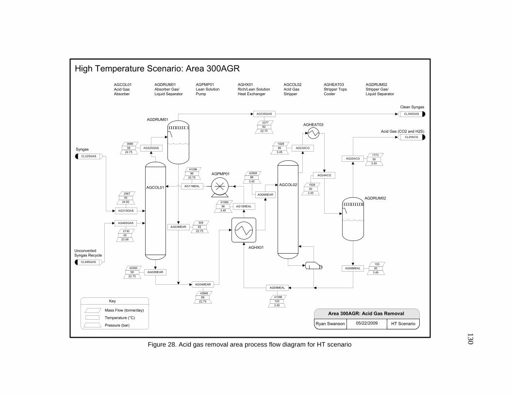
130

Figure 28. Acid gas removal area process flow diagram for HT scenario

Key

Mass Flow (tonne/day)

Temperature (°C)

Pressure (bar)05/22/2009Ryan Swanson HT Scenario

Area 300AGR: Acid Gas Removal

AGCOL01

Acid Gas

Absorber

AGDRUM01

Absorber Gas/

Liquid Separator

AGPMP01

Lean Solution

Pump

AGHX01

Rich/Lean Solution

Heat Exchanger

AGCOL02

Acid Gas

Stripper

AGHEAT03

Stripper Tops

Cooler

High Temperature Scenario: Area 300AGR

CL49SGAS

Unconverted

Syngas Recycle

Clean Syngas

CL25ACG

Acid Gas (CO2 and H2S)

CL32SGAS

Syngas 58

22.75

3685

AGCOL01AGCOL02

AGPMP01

AGHX01

AGHEAT03

CL34SGASAG33SGAS

AG23ACG

AG24ACG

AG25ACG

AG08MEAL

AG09MEALAG04MEAR

AG03MEAR

AG02MEAR

AG49SGAS

AG31SGAS

AG10MEAL

AG11MEAL

50

3.45

1773

86

3.45

1928

62

22.75

3377

50

3.45

1928

50

3.45

155

123

3.45

4109658

22.75

42868

58

22.75

42560

62

22.75

308

96

22.75

41096

40

24.82

2967

45

23.58

2130

96

3.45

41096

AG32SGAS

AG06MEAR

86

3.45

42868

AGDRUM01

AGDRUM02

Stripper Gas/

Liquid Separator

AGDRUM02

131

Figure 29. Sulfur recovery area process flow diagram for HT scenario

Key

Mass Flow (tonne/day)

Temperature (°C)

Pressure (bar)05/22/2009Ryan Swanson HT Scenario

Area 300SUL: LO-CAT Sulfur Recovery

SUCOL01

LO-CAT Absorber

Vessel

SUCOMP01

Air Compressor

SUHEAT01

Air Cooler

SUREAC01

LO-CAT Oxidizer

Vessel

High Temperature Scenario: Area 300SUL

Flue Gas

CL83SUL

Sulfur Cake

CL25ACG

CL95AIR

SUCOL01

SUREAC01

SUCOMP01

Acid Gas (CO2 and H2S)

CL92AIR

Oxygen

CL40CO2

Carbon Dioxide

SU83SUL

SU95AIR

SU26SULSU25ACG

SU40C02

SU92AIR SUHEAT01

SU94AIR

SU93AIR

53

3.45

8

50

3.45

1773

50

7.2

0.2

53

3.45

1765

25

1.01

1.6

100

2.07

7

50

1.93

1.6

50

3.45

2.3

132

Figure 30. Fuel synthesis area process flow diagram for HT scenario

Key

Mass Flow (tonne/day)

Temperature (°C)

Pressure (bar)05/22/2009Ryan Swanson HT Scenario

Area 400: Fuel Synthesis

FSCOMP01

Syngas Booster

Compressor

FSCOMP02

Syngas Recycle

Compressor

FSSEP03

FT Liquids

Absorber

FSREAC01

Fischer-Tropsch

Reactor

High Temperature Scenario: Area 400

Hydrogen

PL50FT

Fischer-Tropsch Liquids

PL48SGAS

PL34SGAS

Syngas

FSSEP02

Pressure Swing

Adsorption Unit

FSHEAT01

Syngas Heater

FSCOMP01

FSHEAT01

FSSEP01

FSSEP02

FSREAC01

FSHEAT03

FSSEP03

FSCOMP02

FSHEAT04

FSDRUM01

PL49SGAS

PL47SGAS

FS37SGAS FS44SGAS

PL90HYD

FS50FT

FS60WAT

FS44FT

FS45FT

FS46SGAS

FS50SGAS

FS51SGAS

FS48SGAS

FS49SGAS

FS47SGAS

FS99CONT

FS36SGAS

FS35SGAS

FS34SGAS

FS90HYD

FS42SGAS

FS40SGAS

FS52SGAS

Water

35

22.20

641

35

22.20

427

35

23.58

4970

200

23.58

4970

42

23.58

3902

42

23.58

1405

50

24.96

1405

45

23.58

156

45

23.58

32.64

45

23.58

2308

200

24.97

0.05

200

26.00

3570

76

26.00

3570

62

22.75

3570

200

1.00

63

200

24.97

67

200

24.97

4

200

24.97

3566

200

24.96

1405

200

24.97

3570

FSSEP01

ZnO/Act. Carbon

Guard Bed

FSHEAT04

Syngas Recycle

Preheater

FSDRUM01

Hydrocarbon/

Oil Separator

FSCOMP03

FS43SGAS237

25.00

63

133

Figure 31. Hydroprocessing area process flow diagram for HT scenario

Key

Mass Flow (tonne/day)

Temperature (°C)

Pressure (bar)05/22/2009Ryan Swanson HT Scenario

Area 500: Hydroprocessing

HYREAC01

Hydroprocessing Unit

High Temperature Scenario: Area 500

Gasoline Fuel

PL81DIES

Diesel Fuel

PL63FT

PL71GASO

HYREAC01

FT Liquids

PL90HYD

Hydrogen

HY81DIES

HY71GASO

HY50FT

HY90HYD

35

22.20

427

50

22.20

267

30

1.00

4.4

50

22.20

112

Fuel Gas

PL65FGASHY65FGAS

50

22.20

53

HYTANK01

HY80DIES

50

22.20

267

HY70GASO

50

22.20

112

HYTANK02

HYTANK01

Diesel Tank

HYTANK02

Gasoline Tank

134

Figure 32. Power generation area process flow diagram for HT scenario

Key

Mass Flow (tonne/day)

Temperature (°C)

Pressure (bar)05/22/2009Ryan Swanson HT Scenario

Area 600: Power Generation

O2COMP

Air Compressor

for Gas Turbine

HPPUMP

High Pressure

Steam pump

High Temperature Scenario: Area 600

PL88FLUE

Flue Gas

PL49SGAS

Unconverted Syngas

CWPUMP

Cool Water PumpCOMBB

Gas Turbine w/

Generator

680

421

25

1.01

2205

45

23.58

144

STMTURB

Steam Turbine w/

Generator

HRSG

Heat Recovery

Steam Generator

O2COMP COMBB

CWPUMP

602

1136

1.00

2414

CW2 85

7.91

838

CWREC

73

0.30

838

615 252

1.00

2414

HRSG

HPSTM2565

173.38

838

STMTURB

HPPUMP

HPSTM1

400

7.91

838

Air

PL65FGAS

Fuel Gas

HY65SGAS

40

22.2

53

135

Figure 33. Air separation unit process flow diagram for HT scenario

Key

Mass Flow (tonne/day)

Temperature (°C)

Pressure (bar)05/22/2009Ryan Swanson HT Scenario

Area 700: Air Separation Unit

COMP1

Air Compressor

w/ intercoolers

GOXCMP

Oxygen

Compressor

High Temperature Scenario: Area 700

Nitrogen

HX-2

Cryogenic Heat

Exchanger System

HIGH-P

High Pressure N2/O2

Separation Column

AIR-1A-170

6.20

2903

LOW-P

Low Pressure N2/O2

Separation Column

GOXCMP

O2LPC

-181

1.2

714

AIR-L20

6.30

2903

COMP1

HIGH-P

AIR-A

32

1.01

2903

Air

LOW-P

HX-2

O2-OUT 16

1.1

714

N2-OUT

16

1.1

2189

PL90OX

Oxygen

O2-OUT2

68

28.00

714

HX-2

136

D.2 Low Temperature Scenario

137

Figure 34. Overall plant area process flow diagram for LT scenario

05/22/2009Ryan Swanson LT Scenario

Overall Plant

Key

Mass Flow (tonne/day)

Temperature (°C)

Pressure (bar)

A100:

Preprocessing

A200:

Gasification

A300: Syngas

Cleaning

A400: Fuel

Synthesis

A500:

Hydroprocessing

A600: Power

Generation

A700: Air

Separation Unit

PL00BMAS

PL08BMAS PL21SGAS

PL90OX

PL34SGAS

PL56FT

PL56SGAS

PL88FLUE

PL71GASO

PL43CO2

PL89AIR PL92NTGN

PL84STM

PL81STM

PL52FLUE

PL60ASH

PL09AIR

PL41CO2

PL83SUL

PL81WAT

PL55SGAS

PL90HYD

25

1.01

2667

PL92WAT

200

1.98

4000

200

1.01

1471

1200

1.01

119

50

1.93

0.7

40

26.17

1380

210

1.00

195831

22.89

169

120

1.98

4000

90

1.01

2222120

1.98

444

100

1.01

1375

25

1.01

2313

243

28.00

180

149

28.00

561

50

3.45

1387

16

1.1

1744

31

22.89

2080

62

22.89

2716

35

21.17

331

60

1.01

3.4

50

22.89

87

870

27.55

2930

PL99AIR

30

1.01

1749

Low Temperature Scenario

Air

Air

Moisture

Biomass

Flue Gas

Sulfur

Scrubber Waste Water

Flue Gas

Air

Gasoline

Carbon Dioxide

Nitrogen

Water to Scrubber

PL80WAT

30

27.57

500

Ash

Steam

PL98STM

204

28.00

352

PL81DIES

50

22.89

206

Diesel

Steam

PL90STM

300

25

1000

PL65FGAS 50

22.89

41

138

Figure 35. Preprocessing area process flow diagram for LT scenario

CHMIX01

Chopper Feed

Bin

CHGRIN01

First-Pass

Chopper

CHSEP01

12-mm Screen

DRDRY01

Rotary

Steam Dryer

GRMIX01

Grinder

Feed Bin

GRGRIN01

Second-Pass

Grinder

GRSEP01

6-mm Screen

05/22/2009Ryan Swanson LT Scenario

Area 100: Preprocessing

Key

Mass Flow (tonne/day)

Temperature (°C)

Pressure (bar)

GR08BMAS

CH00BMAS

90

1.01

2222

25

1.01

2667

Low Temperature Scenario: Area 100

CHGRIN01

CHMIX01

GRGRIN01

GRMIX01

DRDRY01

CH90BMAS

CH03BMAS

DR05BMAS

GR06BMAS

GR90BMAS

DR81STM

DR84STM

120

1.98

4000

90

1.01

797

90

1.01

3019

90

1.01

2222

25

1.01

514

200

1.98

4000

25

1.01

2667

CHSEP01

GRSEP01

DR92WAT

PL08BMAS

PL00BMAS

PL81STM

PL84STM

PL92WAT

120

1.98

444

CH02BMAS25

1.01

3181

Steam

Wet Biomass

Dry Biomass

Steam Recycle

Reject Moisture

139

Figure 36. Gasification area process flow diagram for LT scenario

05/22/2009Ryan Swanson LT Scenario

Area 200: Gasification

Key

Mass Flow (tonne/day)

Temperature (°C)

Pressure (bar)

GSTANK01

Biomass

Receiving Bin

GSREAC01

Low Temp Fluidized

Bed Gasifier

CYCYC01

Primary

Cyclone Train

CYCYC02

Secondary

Cyclone Train

CYMIX02

Char Collection

Hopper

CBREAC01

Combustor

GS07BMAS 90

1.01

2016

Low Temperature Scenario: Area 200

GS90OX 149

28.00

562PL21SGAS

PL07BMAS

PL90OX

PL84STM

PL81STM

Oxygen

Dry Biomass

Syngas

Steam

Steam

GSREAC01

GSTANK02/03

PL43CO2

CYCYC01

CYCYC02

CBREAC01

PL09AIR

PL52FLUE

CYMIX02

PL60ASH

PL46CO2

Carbon Dioxide

Combustor Flue Gas

Air

Ash

GS05SGAS

CY15CHAR

CY16CHAR

CY14SGAS

GS20SGAS

GS52FLUE

GS09AIR

GS43CO2

GS81STM

GS84STM

GS46CO2

91

28.00

171

100

28.00

180

200

1.98

4000

120

1.98

4000

100

1.01

1375

1500

1.01

1471

1300

26.60

2930

1300

26.61

191

1300

26.62

2566

1300

26.60

24

1300

26.61

2954

GS11BMAS

91

28.00

2033

PL98STM

Steam

GS91STM

149

28.00

352

GSTANK01

GS19CHAR 870

1.98

215

CBCYC01/02

CBMIX01

CB61ASH

CB50FLUE

CB62ASH

1500

1.01

1590

1500

1.01

119

1500

1.01

119

GSTANK02/03

Biomass

Lockhopper

CBCYC01/02

Combustor

Cyclone Train

CBMIX02

Ash Collection

Hopper

140

Figure 37. Syngas cleaning area process flow diagram for LT scenario

Key

Mass Flow (tonne/day)

Temperature (°C)

Pressure (bar)05/22/2009Ryan Swanson LT Scenario

Area 300: Syngas Cleaning

CLSEP03

Direct Quench

Syngas Cooler

CLDRUM02

Surge Drum and

Settling Tank

CLMIX01

Wet Gas

Scrubber

CLDRUM01

Tar Settling

Tank

Low Temperature Scenario: Area 300

Water

AirFlue Gas

PL83SUL

PL40SGAS

PL40CO2

PL81WAT

Carbon Dioxide Vent

Sulfur Cake

Clean Syngas

Dirty Water

CL40CO2

CL40SGAS

62

22.89

2716

50

3.45

1567

CLMIX01

A300AGR:

Acid Gas Removal

A300SUL:

LO-CAT Sulfur Recovery

PL12SGAS

Syngas CLHEAT01

CL81WAT

CL29SGAS

CL25ACG

CL95AIRCL92AIR

CL21SGAS

CL25WAT

CL83WAT

CL80H2O

CL25SGAS

CL83SUL

50

2.1

5.6

40

26.17

2198

40

26.17

1380

50

1.93

21

50

3.45

1593

Water

CL80WAT

25

1.01

1

30

27.57

500194

26.86

3078

98

26.86

6000

30

27.55

150

194

26.86

1.8

870

26.60

2930

CLDRUM01

PL55SGAS

Unconverted Syngas

Recycle

CL49SGAS

31

22.89

2080

CLDRUM02

CL01H2O194

27.55

6000

CLHEAT01

CL02H2O150

27.55

6000

Wet Ash/Char

CLHEAT02

CL84WAT

40

26.86

6000

PL43CO2

CO2 to lockhopperCLCOMP01

CL41CO2

50

3.45

1387

CL43CO2

243

28.00

180

CLHEAT01

Quench Water

Cooler

CLHEAT02

Scrubbing Water

Cooler

141

Figure 38. Acid gas removal area process flow diagram for LT scenario

Key

Mass Flow (tonne/day)

Temperature (°C)

Pressure (bar)04/22/2009Ryan Swanson LT Scenario

Area 300AGR: Acid Gas Removal

AGCOL01

Acid Gas

Absorber Column

AGDRUM01

Absorber Knock-

out Drum

AGPMP01

Lean Solution

Pump

AGHX01

Rich/Lean Solution

Heat Exchanger

AGCOL02

Acid Gas Stripper

Column

AGHEAT03

Stripper

Condenser

Low Temperature Scenario: Area 300AGR

CL49SGAS

Unconverted

Syngas Recycle

Clean Syngas

CL25ACG

Acid Gas (CO2 and H2S)

CL29SGAS

Syngas 50

22.89

2925

AGCOL01AGCOL02

AGPMP01

AGHX01

AGHEAT03

CL40SGASAG33SGAS

AG23ACG

AG24ACG

AG25ACG

AG08MEAL

AG09MEALAG04MEAR

AG03MEAR

AG02MEAR

AG49SGAS

AG26SGAS

AG10MEAL

AG11MEAL

50

3.45

1593

93

3.45

1694

62

22.75

1834

50

3.45

1693

50

3.45

101

123

3.45

2728550

22.89

28891

50

22.89

28682

62

22.89

209

96

22.75

33682

40

26.17

2198

31

22.89

2080

96

3.45

33682

AG32SGAS

AG06MEAR

93

3.45

28891

AGDRUM01

AGDRUM02

Stripper Knock-

out drum

AGDRUM02

142

Figure 39. Sulfur recovery process flow diagram for LT scenario

Key

Mass Flow (tonne/day)

Temperature (°C)

Pressure (bar)05/22/2009Ryan Swanson LT Scenario

Area 300SUL: LO-CAT Sulfur Recovery

SUCOL01

LO-CAT Absorber

Vessel

SUREAC01

LO-CAT Oxidizer

Vessel

Low Temperature Scenario: Area 300SUL

Flue Gas

CL83SUL

Sulfur Cake

CL25ACG

CL95AIR

SUCOL01

SUREAC01

Acid Gas (CO2 and H2S)

CL92AIR

Air

CL40CO2

Carbon Dioxide

SU83SUL

SU95AIR

SU26SULSU25ACG

SU40C02

SU92AIR

50

3.45

26

50

3.45

1593

50

3.45

5.6

50

3.45

1567

25

1.01

1.2

50

3.45

21

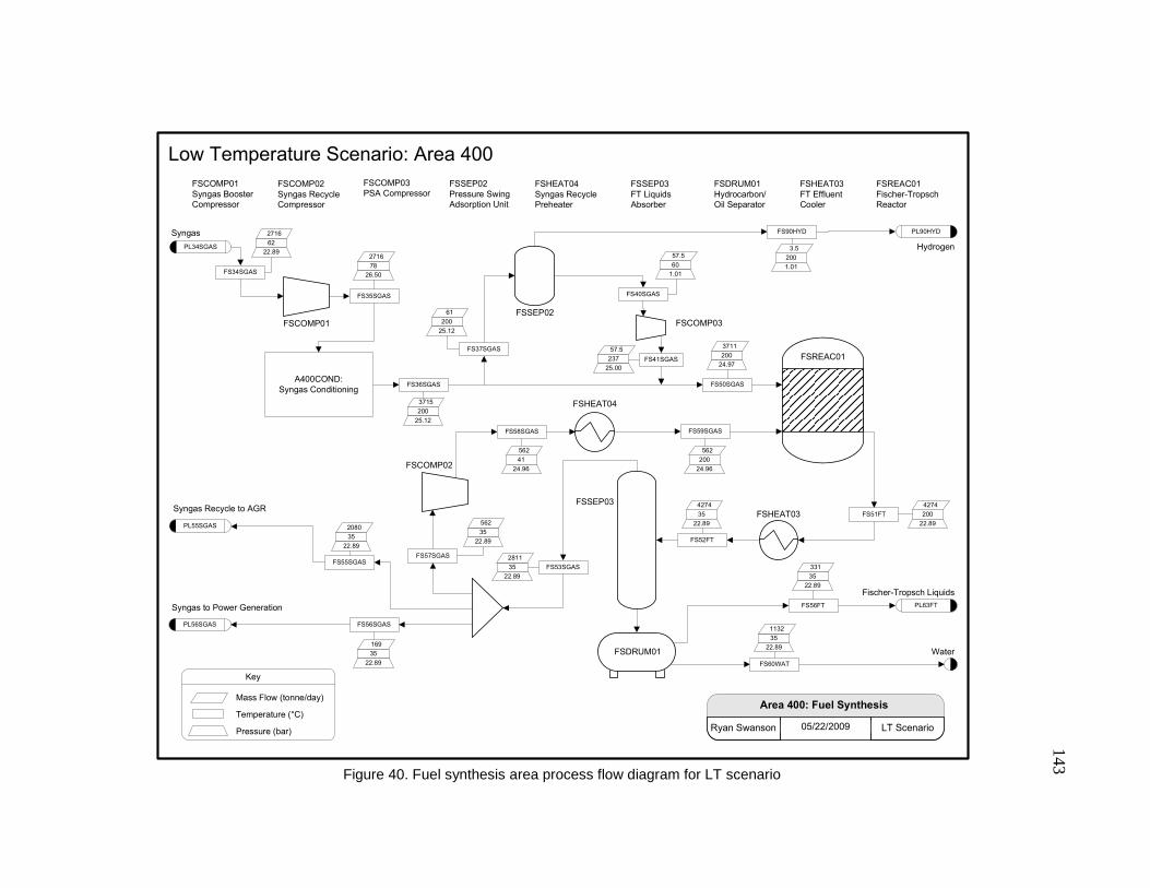
143

Figure 40. Fuel synthesis area process flow diagram for LT scenario

Key

Mass Flow (tonne/day)

Temperature (°C)

Pressure (bar)05/22/2009Ryan Swanson LT Scenario

Area 400: Fuel Synthesis

FSCOMP01

Syngas Booster

Compressor

FSCOMP02

Syngas Recycle

Compressor

FSSEP03

FT Liquids

Absorber

FSREAC01

Fischer-Tropsch

Reactor

Low Temperature Scenario: Area 400

Hydrogen

PL63FT

Fischer-Tropsch Liquids

PL55SGAS

PL34SGAS

Syngas

FSSEP02

Pressure Swing

Adsorption Unit

FSCOMP01

FSSEP02

FSREAC01

FSHEAT03

FSSEP03

FSCOMP02

FSHEAT04

FSDRUM01

PL56SGAS

FS36SGAS FS50SGAS

PL90HYD

FS56FT

FS60WAT

FS51FT

FS52FT

FS53SGAS

FS57SGAS

FS58SGAS

FS55SGAS

FS56SGAS

FS35SGAS

FS34SGAS

FS90HYD

FS40SGAS

FS37SGAS

FS59SGAS

Water

35

22.89

1132

35

22.89

331

35

22.89

4274

200

22.89

4274

35

22.89

2811

35

22.89

562

41

24.96

562

35

22.89

169

35

22.89

2080

78

26.50

2716

62

22.89

2716

60

1.01

57.5

200

25.12

61

200

1.01

3.5

200

24.97

3711

200

24.96

562

200

25.12

3715

FSHEAT04

Syngas Recycle

Preheater

FSDRUM01

Hydrocarbon/

Oil Separator

A400COND:

Syngas Conditioning

FSCOMP03

FS41SGAS237

25.00

57.5

Syngas Recycle to AGR

Syngas to Power Generation

FSCOMP03

PSA CompressorFSHEAT03

FT Effluent

Cooler

144

Figure 41. Syngas conditioning area process flow diagram for LT scenario

Key

Mass Flow (tonne/day)

Temperature (°C)

Pressure (bar)05/22/2009Ryan Swanson LT Scenario

Area 400COND: Syngas Conditioning

CDREAC01

Steam Methane

Reforming Reactor

CDHEAT04

Syngas Cooler

Low Temperature Scenario: Area 400COND

FS36SGAS

Clean Syngas

FS35SGAS

Syngas

CDHEAT03

Syngas Cooler

CDHEAT01

Syngas Heater

CDHEAT01

CDSEP01

CDREAC01

CD38SGAS

CD40SGAS

CD39SGAS

CD44SGAS

CD99CONT

CD36SGAS

CD35SGAS

300

25.81

3715

304

25.12

3715

870

25.81

3715

150

26.50

1.4

150

26.50

2716

62

26.50

2716

870

26.50

2715

CDSEP01

ZnO/Act. Carbon

Guard Bed

CDREAC02

Water Gas Shift

Reactor

CDREAC02

CL42SGAS 315

25.12

927

Steam

CD80STM

200

25.00

1000

CDHEAT02

CD37SGAS

150

26.50

2715

CLHEAT03

CD41SGAS

300

25.81

927

CDHEAT04

CD45SGAS

200

25.12

3715

CDHEAT02

Fired Syngas

Pre-heater

Gas Contaminants

145

Figure 42. Hydroprocessing area process diagram for LT scenario

Key

Mass Flow (tonne/day)

Temperature (°C)

Pressure (bar)05/22/2009Ryan Swanson LT Scenario

Area 500: Hydroprocessing

HYREAC01

Whole

Hydroprocessing Unit

Low Temperature Scenario: Area 500

Gasoline Fuel

PL65DSL

Diesel Fuel

PL56FT

PL64GASO

HYREAC01

FT Liquids

PL90HYD

Hydrogen

HY81DIES

HY71GASO

HY56FT

HY90HYD

35

22.89

331

50

22.89

206

60

24.97

3.4

50

22.89

87

Fuel Gas

PL65FGASHY65FGAS

50

22.89

41

HYTANK02

HY80DIES

50

22.89

206

HY70GASO

50

22.89

87

HYTANK01

HYTANK01

Gasoline Tank

HYTANK02

Diesel Tank

146

Figure 43. Power generation area process flow diagram for LT scenario

Key

Mass Flow (tonne/day)

Temperature (°C)

Pressure (bar)05/22/2009Ryan Swanson LT Scenario

Area 600: Power Generation

O2COMP

Air Compressor

for Gas Turbine

HPPUMP

High Pressure

Steam pump

High Temperature Scenario: Area 600

PL88FLUE

Flue Gas

PL40SGAS

Unconverted Syngas

CWPUMP

Cool Water PumpCOMBB

Gas Turbine w/

Generator

680

421

25

1.01

1749

40

22.2

209

STMTURB

Steam Turbine w/

Generator

HRSG

Heat Recovery

Steam Generator

O2COMP COMBB

CWPUMP

602

1161

1.00

1958

CW2 85

7.91

740

CWREC

73

1.01

740

615 210

1.00

1958

HRSG

HPSTM394

173.38

740

STMTURB

HPPUMP

HPW1

174

7.91

740

Air

PL88FLUE

Fuel Gas

HY65FGAS

50

22.89

41

147

Figure 44. Air separation unit process flow diagram for LT scenario

Key

Mass Flow (tonne/day)

Temperature (°C)

Pressure (bar)05/22/2009Ryan Swanson LT Scenario

Area 700: Air Separation Unit

COMP1

Air Compressor

w/ intercoolers

GOXCMP

Oxygen

Compressor

High Temperature Scenario: Area 700

Nitrogen

HX-2

Cryogenic Heat

Exchanger System

HIGH-P

High Pressure N2/O2

Separation Column

AIR-1A-170

6.20

2313

LOW-P

Low Pressure N2/O2

Separation Column

GOXCMP

O2LPC

-181

1.2

569

AIR-L20

6.30

2313

COMP1

HIGH-P

AIR-A

32

1.01

2313

Air

LOW-P

HX-2

O2-OUT 16

1.1

569

N2-OUT

16

1.1

1744

PL90OX

Oxygen

O2-OUT2

55

28.00

569

HX-2

148

APPENDIX E. STREAM DATA

E.1 High Temperature Scenario

149

Table 39. Overall plant stream data for HT scenario

HT Overall Plant

PL00BMAS

PL08BMAS

PL09CAIRPL17SLAGPL21SGASPL34SGAS

PL42CO2PL43CO2

PL47SGASPL48SGASPL49SGAS

PL50FTPL52FLUEPL65FGASPL71GASOPL81DIESPL81STM

PL81WAT

PL83SULPL84STM

PL88FLUE

PL89AIR

PL90HYD

PL90OXPL90STM

PL92NTGNPL92W

ATPL98STM

PL99AIR

Temperature (C) 25 90 25 50 1300 62 250 53 45 45 45 35 220 35 36 37 200 40 50 120 273 32 30 149 190 -179 120 200 30

Pressure (bar) 1.01 1.01 1.01 26.62 26.62 22.75 28.00 3.45 23.58 23.58 23.58 22.20 1.03 22.20 1.03 1.03 1.98 24.82 1.93 1.98 1.00 1.01 1.00 28.00 10.00 1.20 1.98 28.00 1.01

Vapor Fraction 0.00 0.00 1.00 0.00 1.00 1.00 1.00 1.00 1.00 1.00 1.00 0.00 1.00 1.00 0.00 0.00 1.00 0.00 0.00 1.00 1.00 1.00 1.00 1.00 1.00 1.00 1.00 0.00 1.00

Volume Flow** (m3/sec) 0.43 0.14 2.33 0 11.23 3.45 0.07 3.32 0.02 1.64 0.11 0.01 4.33 0.02 0 0.01 50.53 0.02 0 42.34 45.37 29.07 0.63 0.34 1.30 5.76 4.70 0.02 22.37

Mole Flow** (kmol/hr) 1542 513.97 343.36 0 8192 10089 175.05 1541 71.82 5260 355.46 89.49 393.42 74.55 41.08 48.97 9251 3276 13.46 9251 3595 4177 90.27 957.07 1271 3255 1028 2220 3237

Mass Flow (tonnes/day) 2667 2222 237.82 114.00 3825 3377 180.00 1585 29.08 2130 143.95 427.14 266.91 52.77 112.62 266.11 4000 1501 7.20 4000 2439 2903 4.37 743.70 549.62 2189 444.44 960.00 2242

H2O 666.67 222.22 0 0 988.43 45.53 2.50 21.97 0 0 0 0 27.89 0 0 0 0 1348 4.04 0 233.43 0 0 0 549.62 0 444.44 960.00 0

CO 0 0 0 0 1457 1818 0.47 4.15 11.24 823.54 55.65 0 0 0 0 0 0 22.10 0 0 0 0 0 0 0 0 0 0 0

H2 0 0 0 0 122.88 288.34 0 0 1.83 134.08 9.06 0 0 0 0 0 0 0 0 0 0 0 4.37 0 0 0 0 0 0

CO2 0 0 0 0 1184 190.01 175.21 1543 2.40 175.74 11.88 0 40.00 0 0 0 0 128.26 0 0 352.24 0 0 0 0 0 0 0 0

O2 0 0 55.97 0 0 0 0 0 0 0 0 0 10.28 0 0 0 0 0 0 0 104.25 672.19 0 700.00 0 0 0 0 527.27

N2 0 0 181.85 0 17.68 0 1.78 15.63 0 0 0 0 181.85 0 0 0 0 0.26 0 0 1715 2194 0 0 0 2189 0 0 1715

CH4 0 0 0 0 0.02 63.41 0.01 0.07 0.87 63.47 4.29 0 0 14.94 0 0 0 0 0 0 0 0 0 0 0 0 0 0 0

C2H6 0 0 0 0 0 106.90 0.01 0.10 1.46 107.01 7.23 0 0 0 0 0 0 0 0 0 0 0 0 0 0 0 0 0 0

C2H4 0 0 0 0 0 0 0 0 0 0 0 0 0 0 0 0 0 0 0 0 0 0 0 0 0 0 0 0 0

C2H2 0 0 0 0 0 0 0 0 0 0 0 0 0 0 0 0 0 0 0 0 0 0 0 0 0 0 0 0 0

C3 0 0 0 0 0 141.45 0.01 0.10 1.93 141.56 9.57 0 0 37.83 0 0 0 0 0 0 0 0 0 0 0 0 0 0 0

C4 0 0 0 0 0 167.38 0.02 0.15 2.29 167.55 11.32 0 0 0 0 0 0 0 0 0 0 0 0 0 0 0 0 0 0

H2S 0 0 0 0 4.50 0.03 0 0 0 0 0 0 0 0 0 0 0 1.02 0 0 0 0 0 0 0 0 0 0 0

NH3 0 0 0 0 0.11 0 0 0 0 0 0 0 0 0 0 0 0 0.10 0 0 0 0 0 0 0 0 0 0 0

TAR 0 0 0 0 0 0 0 0 0 0 0 0 0 0 0 0 0 0 0 0 0 0 0 0 0 0 0 0 0

SULFUR 0 0 0 0 0 0 0 0 0 0 0 0 0 0 0 0 0 0 3.16 0 0 0 0 0 0 0 0 0 0

CARBON 0 0 0 0 0 0 0 0 0 0 0 0 0 0 0 0 0 0 0 0 0 0 0 0 0 0 0 0 0

CHAR 0 0 0 0 0 0 0 0 0 0 0 0 0 0 0 0 0 0 0 0 0 0 0 0 0 0 0 0 0

STEAM 0 0 0 0 0 0 0 0 0 0 0 0 0 0 0 0 4000 0 0 4000 0 0 0 0 0 0 0 0 0

SO2 0 0 0 0 0 0 0 0 0 0 0 0 0.02 0 0 0 0 0 0 0 0.08 0 0 0 0 0 0 0 0

NO2 0 0 0 0 0 0 0 0 0 0 0 0 0 0 0 0 0 0 0 0 0 0 0 0 0 0 0 0 0

MEA 0 0 0 0 0 0 0 0 0 0 0 0 0 0 0 0 0 0 0 0 0 0 0 0 0 0 0 0 0

AIR 0 0 0 0 0 0 0 0 0 0 0 0 0 0 0 0 0 0 0 0 0 0 0 0 0 0 0 0 0

WAXES 0 0 0 0 0 0 0 0 0 0 0 170.22 0 0 0 0 0 0 0 0 0 0 0 0 0 0 0 0 0

C5 0 0 0 0 0 2.29 0 0 0.03 2.29 0.15 15.49 0 0 0 0 0 0 0 0 0 0 0 0 0 0 0 0 0

C6 0 0 0 0 0 2.46 0 0 0.03 2.46 0.17 16.65 0 0 0 0 0 0 0 0 0 0 0 0 0 0 0 0 0

C7 0 0 0 0 0 1.15 0 0 0.02 1.15 0.08 17.54 0 0 0 0 0 0 0 0 0 0 0 0 0 0 0 0 0

C8 0 0 0 0 0 1.18 0 0 0.02 1.18 0.08 17.99 0 0 112.62 0 0 0 0 0 0 0 0 0 0 0 0 0 0

C9 0 0 0 0 0 1.11 0 0 0.02 1.19 0.08 18.10 0 0 0 0 0 0 0 0 0 0 0 0 0 0 0 0 0

C10 0 0 0 0 0 1.16 0 0 0.02 1.19 0.08 18.12 0 0 0 0 0 0 0 0 0 0 0 0 0 0 0 0 0

C11 0 0 0 0 0 0.83 0 0 0.02 1.16 0.08 17.62 0 0 0 0 0 0 0 0 0 0 0 0 0 0 0 0 0

C12 0 0 0 0 0 0.13 0 0 0.01 0.54 0.04 17.25 0 0 0 0 0 0 0 0 0 0 0 0 0 0 0 0 0

C13 0 0 0 0 0 0.02 0 0 0.01 0.52 0.04 16.70 0 0 0 0 0 0 0 0 0 0 0 0 0 0 0 0 0

C14 0 0 0 0 0 0 0 0 0.01 0.50 0.03 16.16 0 0 0 0 0 0 0 0 0 0 0 0 0 0 0 0 0

C15 0 0 0 0 0 0 0 0 0.01 0.49 0.03 15.57 0 0 0 0 0 0 0 0 0 0 0 0 0 0 0 0 0

C16 0 0 0 0 0 0 0 0 0.01 0.47 0.03 14.93 0 0 0 266.11 0 0 0 0 0 0 0 0 0 0 0 0 0

C17 0 0 0 0 0 0 0 0 0 0 0 14.75 0 0 0 0 0 0 0 0 0 0 0 0 0 0 0 0 0

C18 0 0 0 0 0 0 0 0 0 0 0 14.05 0 0 0 0 0 0 0 0 0 0 0 0 0 0 0 0 0

C19 0 0 0 0 0 0 0 0 0 0 0 13.35 0 0 0 0 0 0 0 0 0 0 0 0 0 0 0 0 0

C20 0 0 0 0 0 0 0 0 0 0 0 12.64 0 0 0 0 0 0 0 0 0 0 0 0 0 0 0 0 0

COS 0 0 0 0 0.30 1.20 0 0 0.02 1.12 0.08 0 0 0 0 0 0 0.13 0 0 0 0 0 0 0 0 0 0 0

AR 0 0 0 0 43.70 544.37 0 0 6.87 502.93 33.99 0 6.87 0 0 0 0 1.03 0 0 33.99 37.28 0 43.70 0 0.12 0 0 0

BIOMASS 2000 2000 0 0 0 0 0 0 0 0 0 0 0 0 0 0 0 0 0 0 0 0 0 0 0 0 0 0 0

ASH 0 0 0 0 0 0 0 0 0 0 0 0 0 0 0 0 0 0 0 0 0 0 0 0 0 0 0 0 0

SOOT 0 0 0 0 6.00 0 0 0 0 0 0 0 0 0 0 0 0 0 0 0 0 0 0 0 0 0 0 0 0

SLAG 0 0 0 114.00 0 0 0 0 0 0 0 0 0 0 0 0 0 0 0 0 0 0 0 0 0 0 0 0 0

**Volumetric and Mole flow values do not include biomass, ash, soot, or slag

150

Table 40. Preprocessing area stream data for HT scenario

HT A100

CH00BMAS

CH02BMAS

CH03BMAS

CH90BMAS

DR05BMAS

DR81STM

DR84STM

DR92WAT

GR06BMAS

GR08BMAS

GR90BMAS

Temperature (C) 25 25 25 25 90 200 120 120 90 90 90

Pressure (bar) 1.01 1.01 1.01 1.01 1.01 1.98 1.98 1.98 1.01 1.01 1.01

Vapor Fraction 0.00 0.00 0.00 0.00 0.00 1.00 1.00 1.00 0.00 0.00 0.00

Volume Flow** (m3/sec) 0.43 0.43 0.43 0 0.14 50.53 42.34 4.70 0.14 0.14 0

Mole Flow** (kmol/hr) 1542 1542 1542 0 513.97 9251 9251 1028 513.97 513.97 0

Mass Flow (tonnes/day) 2667 2709 2667 42.20 2222 4000 4000 444.44 2240 2222 17.60

H2O 666.67 666.67 666.67 0 222.22 0 0 444.44 222.22 222.22 0

CO 0 0 0 0 0 0 0 0 0 0 0

H2 0 0 0 0 0 0 0 0 0 0 0

CO2 0 0 0 0 0 0 0 0 0 0 0

O2 0 0 0 0 0 0 0 0 0 0 0

N2 0 0 0 0 0 0 0 0 0 0 0

CH4 0 0 0 0 0 0 0 0 0 0 0

C2H6 0 0 0 0 0 0 0 0 0 0 0

C2H4 0 0 0 0 0 0 0 0 0 0 0

C2H2 0 0 0 0 0 0 0 0 0 0 0

C3 0 0 0 0 0 0 0 0 0 0 0

C4 0 0 0 0 0 0 0 0 0 0 0

H2S 0 0 0 0 0 0 0 0 0 0 0

NH3 0 0 0 0 0 0 0 0 0 0 0

TAR 0 0 0 0 0 0 0 0 0 0 0

SULFUR 0 0 0 0 0 0 0 0 0 0 0

CARBON 0 0 0 0 0 0 0 0 0 0 0

CHAR 0 0 0 0 0 0 0 0 0 0 0

STEAM 0 0 0 0 0 4000 4000 0 0 0 0

SO2 0 0 0 0 0 0 0 0 0 0 0

NO2 0 0 0 0 0 0 0 0 0 0 0

MEA 0 0 0 0 0 0 0 0 0 0 0

AIR 0 0 0 0 0 0 0 0 0 0 0

WAXES 0 0 0 0 0 0 0 0 0 0 0

C5 0 0 0 0 0 0 0 0 0 0 0

C6 0 0 0 0 0 0 0 0 0 0 0

C7 0 0 0 0 0 0 0 0 0 0 0

C8 0 0 0 0 0 0 0 0 0 0 0

C9 0 0 0 0 0 0 0 0 0 0 0

C10 0 0 0 0 0 0 0 0 0 0 0

C11 0 0 0 0 0 0 0 0 0 0 0

C12 0 0 0 0 0 0 0 0 0 0 0

C13 0 0 0 0 0 0 0 0 0 0 0

C14 0 0 0 0 0 0 0 0 0 0 0

C15 0 0 0 0 0 0 0 0 0 0 0

C16 0 0 0 0 0 0 0 0 0 0 0

C17 0 0 0 0 0 0 0 0 0 0 0

C18 0 0 0 0 0 0 0 0 0 0 0

C19 0 0 0 0 0 0 0 0 0 0 0

C20 0 0 0 0 0 0 0 0 0 0 0

COS 0 0 0 0 0 0 0 0 0 0 0

AR 0 0 0 0 0 0 0 0 0 0 0

BIOMASS 2000 2042 2000 42.20 2000 0 0 0 2018 2000 17.60

ASH 0 0 0 0 0 0 0 0 0 0 0

SOOT 0 0 0 0 0 0 0 0 0 0 0

SLAG 0 0 0 0 0 0 0 0 0 0 0

**Volumetric and Mole flow values do not include biomass, ash, soot, or slag

151

Table 41. Gasification area stream data for HT scenario

HT A200

GS02SLAG

GS08BMAS

GS09CAIR

GS11BMAS

GS42CO2

GS52FLUE

GS54SGAS

GS81STM

GS84STM

GS90OX

GS92CO2

GS98STM

S06SGAS

SL01SLAG

SL02SGAS

Temperature (C) 50 90 25 90 250 220 45 200 120 149 92 200 203 1300 1300

Pressure (bar) 26.62 1.01 1.01 1.01 28.00 1.03 23.58 1.98 1.98 28.00 28.00 28.00 25.93 26.62 26.62

Vapor Fraction 0.00 0.00 1.00 0.53 1.00 1.00 1.00 1.00 1.00 1.00 1.00 0.00 1.00 0.00 1.00

Volume Flow** (m3/sec) 0 0.14 2.33 30.59 0.07 4.33 0.02 50.53 42.34 0.34 0.04 0.02 3.50 0 11.23

Mole Flow** (kmol/hr) 0 513.97 343.36 6974 175.05 393.42 71.82 9251 9251 957.07 158.25 2220 8308 0 8192

Mass Flow (tonnes/day) 114.00 2222 237.82 2222 180.00 266.91 29.08 4000 4000 743.70 166.90 960.00 3869 114.00 3825

H2O 0 222.22 0 222.22 2.50 27.89 0 0 0 0 0 960.00 1038 0 988.43

CO 0 0 0 0 0.47 0 11.24 0 0 0 0.45 0 1457 0 1457

H2 0 0 0 101.20 0 0 1.83 0 0 0 0 0 122.88 0 122.88

CO2 0 0 0 0 175.21 40.00 2.40 0 0 0 166.45 0 1184 0 1184

O2 0 0 55.97 812.60 0 10.28 0 0 0 700.00 0 0 0 0 0

N2 0 0 181.85 16.00 1.78 181.85 0 0 0 0 0 0 17.68 0 17.68

CH4 0 0 0 0 0.01 0 0.87 0 0 0 0 0 0.02 0 0.02

C2H6 0 0 0 0 0.01 0 1.46 0 0 0 0 0 0 0 0

C2H4 0 0 0 0 0 0 0 0 0 0 0 0 0 0 0

C2H2 0 0 0 0 0 0 0 0 0 0 0 0 0 0 0

C3 0 0 0 0 0.01 0 1.93 0 0 0 0 0 0 0 0

C4 0 0 0 0 0.02 0 2.29 0 0 0 0 0 0 0 0

H2S 0 0 0 0 0 0 0 0 0 0 0 0 4.50 0 4.50

NH3 0 0 0 0 0 0 0 0 0 0 0 0 0.11 0 0.11

TAR 0 0 0 0 0 0 0 0 0 0 0 0 0 0 0

SULFUR 0 0 0 4.40 0 0 0 0 0 0 0 0 0 0 0

CARBON 0 0 0 945.60 0 0 0 0 0 0 0 0 0 0 0

CHAR 0 0 0 0 0 0 0 0 0 0 0 0 0 0 0

STEAM 0 0 0 0 0 0 0 4000 4000 0 0 0 0 0 0

SO2 0 0 0 0 0 0.02 0 0 0 0 0 0 0 0 0

NO2 0 0 0 0 0 0 0 0 0 0 0 0 0 0 0

MEA 0 0 0 0 0 0 0 0 0 0 0 0 0 0 0

AIR 0 0 0 0 0 0 0 0 0 0 0 0 0 0 0

WAXES 0 0 0 0 0 0 0 0 0 0 0 0 0 0 0

C5 0 0 0 0 0 0 0.03 0 0 0 0 0 0 0 0

C6 0 0 0 0 0 0 0.03 0 0 0 0 0 0 0 0

C7 0 0 0 0 0 0 0.02 0 0 0 0 0 0 0 0

C8 0 0 0 0 0 0 0.02 0 0 0 0 0 0 0 0

C9 0 0 0 0 0 0 0.02 0 0 0 0 0 0 0 0

C10 0 0 0 0 0 0 0.02 0 0 0 0 0 0 0 0

C11 0 0 0 0 0 0 0.02 0 0 0 0 0 0 0 0

C12 0 0 0 0 0 0 0.01 0 0 0 0 0 0 0 0

C13 0 0 0 0 0 0 0.01 0 0 0 0 0 0 0 0

C14 0 0 0 0 0 0 0.01 0 0 0 0 0 0 0 0

C15 0 0 0 0 0 0 0.01 0 0 0 0 0 0 0 0

C16 0 0 0 0 0 0 0.01 0 0 0 0 0 0 0 0

C17 0 0 0 0 0 0 0 0 0 0 0 0 0 0 0

C18 0 0 0 0 0 0 0 0 0 0 0 0 0 0 0

C19 0 0 0 0 0 0 0 0 0 0 0 0 0 0 0

C20 0 0 0 0 0 0 0 0 0 0 0 0 0 0 0

COS 0 0 0 0 0 0 0.02 0 0 0 0 0 0.30 0 0.30

AR 0 0 0 0 0 6.87 6.87 0 0 43.70 0 0 43.70 0 43.70

BIOMASS 0 2000 0 0 0 0 0 0 0 0 0 0 0 0 0

ASH 0 0 0 120.00 0 0 0 0 0 0 0 0 0 0 0

SOOT 0 0 0 0 0 0 0 0 0 0 0 0 0 0 6.00

SLAG 114.00 0 0 0 0 0 0 0 0 0 0 0 0 114.00 0

**Volumetric and Mole flow values do not include biomass, ash, soot, or slag

152

Table 42. Syngas cleaning area stream data for HT scenario

HT A300

CL25ACGCL25SGASCL26SGASCL28SGASCL29SGASCL32SGAS

CL40CO2CL41CO2CL42CO2

CL49SGASCL81W

ATCL82W

AT

CL83SULCL83W

ATCL90STM

CL92AIR

CL95AIRGS84STMSG91STM

SL01H2OSL02SGAS

SL03H2O

SL80H2O

Temperature (C) 50 203 291 240 60 40 53 53 250 45 30 40 50 60 190 25 50 62 250 203 1300 203 30

Pressure (bar) 3.45 25.93 24.82 24.82 24.82 24.82 3.45 3.45 28.00 23.58 24.82 24.82 1.93 24.82 10.00 1.01 1.93 22.75 25.86 26.62 26.62 25.93 26.62

Vapor Fraction 1.00 1.00 1.00 1.00 0.69 1.00 1.00 1.00 1.00 1.00 0.00 0.00 0.00 0.00 1.00 1.00 0.93 1.00 1.00 0.00 1.00 0.00 0.00

Volume Flow** (m3/sec) 3.69 1.08 2.01 4.54 2.07 1.86 3.70 0.38 0.07 1.64 0 0.02 0 0.02 1.30 0.01 0.01 3.45 0.54 0.07 11.23 0 0

Mole Flow** (kmol/hr) 1728 2576 3847 9579 9579 6419 1716 175.05 175.05 5260 115.64 3276 13.46 2313 1271 2.07 2.58 10089 1271 9251 8192 0 115.64

Mass Flow (tonnes/day) 1773 1199 1749 4418 4418 2967 1765 180.00 180.00 2130 50.00 1501 7.20 1000 549.62 1.59 2.32 3377 549.62 4000 3825 6.00 50.00

H2O 27.18 321.91 591.14 1308 1308 9.19 24.46 2.50 2.50 0 50.00 1348 4.04 1000 549.62 0 0.45 45.53 549.62 4000 988.43 0 50.00

CO 4.62 451.69 15.74 1021 1021 999.01 4.62 0.47 0.47 823.54 0 22.10 0 0 0 0 0 1818 0 0 1457 0 0

H2 0 38.09 69.47 154.26 154.26 154.26 0 0 0 134.08 0 0 0 0 0 0 0 288.34 0 0 122.88 0 0

CO2 1718 367.08 1052 1869 1869 1741 1718 175.21 175.21 175.74 0 128.26 0 0 0 0 0 190.01 0 0 1184 0 0

O2 0 0 0 0 0 0 0 0 0 0 0 0 0 0 0 1.59 0.02 0 0 0 0 0 0

N2 17.41 5.48 5.48 17.68 17.68 17.43 17.41 1.78 1.78 0 0 0.26 0 0 0 0 0 0 0 0 17.68 0 0

CH4 0.08 0.01 0.01 0.02 0.02 0.02 0.08 0.01 0.01 63.47 0 0 0 0 0 0 0 63.41 0 0 0.02 0 0

C2H6 0.11 0 0 0 0 0 0.11 0.01 0.01 107.01 0 0 0 0 0 0 0 106.90 0 0 0 0 0

C2H4 0 0 0 0 0 0 0 0 0 0 0 0 0 0 0 0 0 0 0 0 0 0 0

C2H2 0 0 0 0 0 0 0 0 0 0 0 0 0 0 0 0 0 0 0 0 0 0 0

C3 0.11 0 0 0 0 0 0.11 0.01 0.01 141.56 0 0 0 0 0 0 0 141.45 0 0 0 0 0

C4 0.17 0 0 0 0 0 0.17 0.02 0.02 167.55 0 0 0 0 0 0 0 167.38 0 0 0 0 0

H2S 3.39 1.40 1.40 4.50 4.50 3.48 0 0 0 0 0 1.02 0 0 0 0 0.03 0.03 0 0 4.50 0 0

NH3 0 0.03 0.03 0.11 0.11 0.01 0 0 0 0 0 0.10 0 0 0 0 0 0 0 0 0.11 0 0

TAR 0 0 0 0 0 0 0 0 0 0 0 0 0 0 0 0 0 0 0 0 0 0 0

SULFUR 0 0 0 0 0 0 0 0 0 0 0 0 3.16 0 0 0 0 0 0 0 0 0 0

CARBON 0 0 0 0 0 0 0 0 0 0 0 0 0 0 0 0 0 0 0 0 0 0 0

CHAR 0 0 0 0 0 0 0 0 0 0 0 0 0 0 0 0 0 0 0 0 0 0 0

STEAM 0 0 0 0 0 0 0 0 0 0 0 0 0 0 0 0 0 0 0 0 0 0 0

SO2 0 0 0 0 0 0 0 0 0 0 0 0 0 0 0 0 0 0 0 0 0 0 0

NO2 0 0 0 0 0 0 0 0 0 0 0 0 0 0 0 0 0 0 0 0 0 0 0

MEA 0 0 0 0 0 0 0 0 0 0 0 0 0 0 0 0 0 0 0 0 0 0 0

AIR 0 0 0 0 0 0 0 0 0 0 0 0 0 0 0 0 0 0 0 0 0 0 0

WAXES 0 0 0 0 0 0 0 0 0 0 0 0 0 0 0 0 0 0 0 0 0 0 0

C5 0 0 0 0 0 0 0 0 0 2.29 0 0 0 0 0 0 0 2.29 0 0 0 0 0

C6 0 0 0 0 0 0 0 0 0 2.46 0 0 0 0 0 0 0 2.46 0 0 0 0 0

C7 0 0 0 0 0 0 0 0 0 1.15 0 0 0 0 0 0 0 1.15 0 0 0 0 0

C8 0 0 0 0 0 0 0 0 0 1.18 0 0 0 0 0 0 0 1.18 0 0 0 0 0

C9 0.08 0 0 0 0 0 0 0 0 1.19 0 0 0 0 0 0 0.08 1.11 0 0 0 0 0

C10 0.03 0 0 0 0 0 0 0 0 1.19 0 0 0 0 0 0 0.03 1.16 0 0 0 0 0

C11 0.23 0 0 0 0 0 0 0 0 1.16 0 0 0 0 0 0 0.23 0.83 0 0 0 0 0

C12 0.13 0 0 0 0 0 0 0 0 0.54 0 0 0 0 0 0 0.13 0.13 0 0 0 0 0

C13 0.04 0 0 0 0 0 0 0 0 0.52 0 0 0 0 0 0 0.04 0.02 0 0 0 0 0

C14 0.01 0 0 0 0 0 0 0 0 0.50 0 0 0 0 0 0 0.01 0 0 0 0 0 0

C15 0 0 0 0 0 0 0 0 0 0.49 0 0 0 0 0 0 0 0 0 0 0 0 0

C16 0 0 0 0 0 0 0 0 0 0.47 0 0 0 0 0 0 0 0 0 0 0 0 0

C17 0 0 0 0 0 0 0 0 0 0 0 0 0 0 0 0 0 0 0 0 0 0 0

C18 0 0 0 0 0 0 0 0 0 0 0 0 0 0 0 0 0 0 0 0 0 0 0

C19 0 0 0 0 0 0 0 0 0 0 0 0 0 0 0 0 0 0 0 0 0 0 0

C20 0 0 0 0 0 0 0 0 0 0 0 0 0 0 0 0 0 0 0 0 0 0 0

COS 0.08 0.09 0.09 0.30 0.30 0.17 0 0 0 1.12 0 0.13 0 0 0 0 0.08 1.20 0 0 0.30 0 0

AR 1.22 13.55 13.55 43.70 43.70 42.66 0 0 0 502.93 0 1.03 0 0 0 0 1.22 544.37 0 0 43.70 0 0

BIOMASS 0 0 0 0 0 0 0 0 0 0 0 0 0 0 0 0 0 0 0 0 0 0 0

ASH 0 0 0 0 0 0 0 0 0 0 0 0 0 0 0 0 0 0 0 0 0 0 0

SOOT 0 0 0 0 0 0 0 0 0 0 0 0 0 0 0 0 0 0 0 0 6.00 6.00 0

SLAG 0 0 0 0 0 0 0 0 0 0 0 0 0 0 0 0 0 0 0 0 0 0 0

**Volumetric and Mole flow values do not include biomass, ash, soot, or slag

153

Table 43. Acid gas removal and sulfur recovery areas stream data for HT scenario

HT A300AGR

AG02MEARAG03MEARAG04MEARAG06MEARAG08MEALAG09MEALAG10MEALAG11MEALAG23ACG

AG24ACG

AG25ACGAG31SGASAG32SGASAG33SGASAG49SGAS A300SUL

SU25ACG

SU26SUL

SU40CO2

SU83SUL

SU92AIR

SU93AIR

SU94AIR

SU95AIR

Temperature (C) 58 62 58 86 50 123 96 96 86 50 50 40 58 62 45 50 53 53 50 25 100 50 50

Pressure (bar) 22.75 22.75 22.75 3.45 3.45 3.45 3.45 20.68 3.45 3.45 3.45 24.82 22.75 22.75 23.58 3.45 3.45 3.45 1.93 1.01 2.07 1.93 1.93

Vapor Fraction 0.00 0.00 0.00 0.01 0.00 0.00 0.00 0.00 0.98 0.83 1.00 1.00 0.93 1.00 1.00 1.00 0.49 1.00 0.00 1.00 1.00 1.00 0.93

Volume Flow** (m3/sec) 0.480 0 0.480 1.590 0 0.480 0.470 0.470 4.820 3.690 3.690 1.860 3.410 3.450 1.640 3.690 0.010 3.700 0 0.010 0.010 0.010 0.010

Mole Flow** (kmol/hr) 84877 699.000 85576 85576 342.110 83848 83848 83848 2070 2070 1728 6419 10788 10089 5260 1728 11.910 1716 13.460 2.070 2.070 2.070 2.580

Mass Flow (tonnes/day) 42560 308.340 42868 42868 155.170 41096 41096 41096 1928 1928 1773 2967 3685 3377 2130 1773 7.930 1765 7.200 1.590 1.590 1.590 2.320

H2O 33956 297.460 34254 34254 144.090 34226 34226 34226 171.270 171.270 27.180 9.190 342.990 45.530 0 27.180 2.720 24.460 4.040 0 0 0 0.450

CO 0 4.640 4.640 4.640 0.010 0.010 0.010 0.010 4.630 4.630 4.620 999.010 1823 1818 823.540 4.620 0 4.620 0 0 0 0 0

H2 0 0 0 0 0 0 0 0 0 0 0 154.260 288.340 288.340 134.080 0 0 0 0 0 0 0 0

CO2 1725 1.650 1727 1727 8.690 8.690 8.690 8.690 1727 1727 1718 1741 191.660 190.010 175.740 1718 0 1718 0 0 0 0 0

O2 0 0 0 0 0 0 0 0 0 0 0 0 0 0 0 0 0 0 0 1.590 1.590 1.590 0.020

N2 17.430 0 17.430 17.430 0.020 0.020 0.020 0.020 17.430 17.430 17.410 17.430 0 0 0 17.410 0 17.410 0 0 0 0 0

CH4 0 0.080 0.080 0.080 0 0 0 0 0.080 0.080 0.080 0.020 63.490 63.410 63.470 0.080 0 0.080 0 0 0 0 0

C2H6 0 0.110 0.110 0.110 0 0 0 0 0.110 0.110 0.110 0 107.010 106.900 107.010 0.110 0 0.110 0 0 0 0 0

C2H4 0 0 0 0 0 0 0 0 0 0 0 0 0 0 0 0 0 0 0 0 0 0 0

C2H2 0 0 0 0 0 0 0 0 0 0 0 0 0 0 0 0 0 0 0 0 0 0 0

C3 0 0.110 0.110 0.110 0 0 0 0 0.110 0.110 0.110 0 141.560 141.450 141.560 0.110 0 0.110 0 0 0 0 0

C4 0 0.170 0.170 0.170 0 0 0 0 0.170 0.170 0.170 0 167.550 167.380 167.550 0.170 0 0.170 0 0 0 0 0

H2S 3.450 0 3.450 3.450 0.060 0.060 0.060 0.060 3.450 3.450 3.390 3.480 0.030 0.030 0 3.390 3.390 0 0 0 0 0 0.030

NH3 0.010 0 0.010 0.010 0.010 0.010 0.010 0.010 0.010 0.010 0 0.010 0 0 0 0 0 0 0 0 0 0 0

TAR 0 0 0 0 0 0 0 0 0 0 0 0 0 0 0 0 0 0 0 0 0 0 0

SULFUR 0 0 0 0 0 0 0 0 0 0 0 0 0 0 0 0 0 0 3.160 0 0 0 0

CARBON 0 0 0 0 0 0 0 0 0 0 0 0 0 0 0 0 0 0 0 0 0 0 0

CHAR 0 0 0 0 0 0 0 0 0 0 0 0 0 0 0 0 0 0 0 0 0 0 0

STEAM 0 0 0 0 0 0 0 0 0 0 0 0 0 0 0 0 0 0 0 0 0 0 0

SO2 0 0 0 0 0 0 0 0 0 0 0 0 0 0 0 0 0 0 0 0 0 0 0

NO2 0 0 0 0 0 0 0 0 0 0 0 0 0 0 0 0 0 0 0 0 0 0 0

MEA 6858 0 6858 6858 0 6858 6858 6858 0 0 0 0 0 0 0 0 0 0 0 0 0 0 0

AIR 0 0 0 0 0 0 0 0 0 0 0 0 0 0 0 0 0 0 0 0 0 0 0

WAXES 0 0 0 0 0 0 0 0 0 0 0 0 0 0 0 0 0 0 0 0 0 0 0

C5 0 0 0 0 0 0 0 0 0 0 0 0 2.290 2.290 2.290 0 0 0 0 0 0 0 0

C6 0 0 0 0 0 0 0 0 0 0 0 0 2.460 2.460 2.460 0 0 0 0 0 0 0 0

C7 0 0 0 0 0 0 0 0 0 0 0 0 1.150 1.150 1.150 0 0 0 0 0 0 0 0

C8 0 0 0 0 0 0 0 0 0 0 0 0 1.180 1.180 1.180 0 0 0 0 0 0 0 0

C9 0 0.080 0.080 0.080 0.010 0.010 0.010 0.010 0.080 0.080 0.080 0 1.190 1.110 1.190 0.080 0.080 0 0 0 0 0 0.080

C10 0 0.030 0.030 0.030 0 0 0 0 0.030 0.030 0.030 0 1.190 1.160 1.190 0.030 0.030 0 0 0 0 0 0.030

C11 0 0.330 0.330 0.330 0.100 0.100 0.100 0.100 0.320 0.320 0.230 0 1.160 0.830 1.160 0.230 0.230 0 0 0 0 0 0.230

C12 0 0.410 0.410 0.410 0.280 0.280 0.280 0.280 0.410 0.410 0.130 0 0.540 0.130 0.540 0.130 0.130 0 0 0 0 0 0.130

C13 0 0.500 0.500 0.500 0.460 0.460 0.460 0.460 0.500 0.500 0.040 0 0.520 0.020 0.520 0.040 0.040 0 0 0 0 0 0.040

C14 0 0.500 0.500 0.500 0.490 0.490 0.490 0.490 0.500 0.500 0.010 0 0.500 0 0.500 0.010 0.010 0 0 0 0 0 0.010

C15 0 0.490 0.490 0.490 0.490 0.490 0.490 0.490 0.490 0.490 0 0 0.490 0 0.490 0 0 0 0 0 0 0 0

C16 0 0.470 0.470 0.470 0.470 0.470 0.470 0.470 0.470 0.470 0 0 0.470 0 0.470 0 0 0 0 0 0 0 0

C17 0 0 0 0 0 0 0 0 0 0 0 0 0 0 0 0 0 0 0 0 0 0 0

C18 0 0 0 0 0 0 0 0 0 0 0 0 0 0 0 0 0 0 0 0 0 0 0

C19 0 0 0 0 0 0 0 0 0 0 0 0 0 0 0 0 0 0 0 0 0 0 0

C20 0 0 0 0 0 0 0 0 0 0 0 0 0 0 0 0 0 0 0 0 0 0 0

COS 0 0.080 0.080 0.080 0 0 0 0 0.080 0.080 0.080 0.170 1.290 1.200 1.120 0.080 0.080 0 0 0 0 0 0.080

AR 0 1.220 1.220 1.220 0 0 0 0 1.220 1.220 1.220 42.660 545.590 544.370 502.930 1.220 1.220 0 0 0 0 0 1.220

BIOMASS 0 0 0 0 0 0 0 0 0 0 0 0 0 0 0 0 0 0 0 0 0 0 0

ASH 0 0 0 0 0 0 0 0 0 0 0 0 0 0 0 0 0 0 0 0 0 0 0

SOOT 0 0 0 0 0 0 0 0 0 0 0 0 0 0 0 0 0 0 0 0 0 0 0

SLAG 0 0 0 0 0 0 0 0 0 0 0 0 0 0 0 0 0 0 0 0 0 0 0

**Volumetric and Mole flow values do not include biomass, ash, soot, or slag

154

Table 44. Fuel synthesis area stream data for HT scenario

HT A400

FS34SGASFS35SGASFS36SGASFS37SGASFS40SGASFS42SGASFS43SGAS

FS44FTFS44SGAS

FS45FTFS45SGAS

FS46FTFS46SGASFS47SGASFS48SGASFS49SGAS

FS50FTFS50SGASFS51SGASFS52SGASFS60W

AT

FS89HYD

FS90HYDFS99CONT

Temperature (C) 62 76 200 200 30 30 417 200 202 35 202 43 0 45 45 45 35 45 50 200 35 30 30 200

Pressure (bar) 22.75 26.00 26.00 24.97 1.00 1.00 24.97 23.58 24.97 23.58 24.96 23.58 0.00 23.58 23.58 23.58 22.20 23.58 24.96 24.96 22.20 1.00 1.00 24.97

Vapor Fraction 1.00 1.00 1.00 1.00 1.00 1.00 1.00 1.00 1.00 0.86 1.00 0.00 1.00 1.00 1.00 1.00 0.00 1.00 1.00 1.00 0.00 1.00 1.00 1.00

Volume Flow** (m3/sec) 3.45 3.16 4.29 4.47 1.26 0.63 0.06 4.84 4.45 2.71 5.86 0.02 2.74 0.02 1.64 0.11 0.01 1.00 0.96 1.42 0.01 0.63 0.63 0

Mole Flow** (kmol/hr) 10089 10089 10089 10089 179.78 89.51 89.51 10438 9998 10438 13198 1575 8887 71.82 5260 355.46 89.49 3199 3199 3199 1483 90.27 90.27 0.04

Mass Flow (tonnes/day) 3377 3377 3377 3377 60.18 55.81 55.81 4668 3372 4668 4668 1069 3599 29.08 2130 143.95 427.14 1296 1296 1296 641.34 4.37 4.37 0.03

H2O 45.53 45.53 45.53 45.53 0.81 0.81 0.81 642.07 45.53 642.07 45.53 642.07 0 0 0 0 0 0 0 0 641.34 0 0 0

CO 1818 1818 1818 1818 32.40 32.40 32.40 1391 1818 1391 2319 0 1391 11.24 823.54 55.65 0 500.87 500.87 500.87 0 0 0 0

H2 288.34 288.34 288.34 288.34 5.14 0.77 0.77 225.34 283.97 225.34 365.52 0 226.52 1.83 134.08 9.06 0 81.55 81.55 81.55 0 4.37 4.37 0

CO2 190.01 190.01 190.01 190.01 3.39 3.39 3.39 296.89 190.01 296.89 296.89 0 296.90 2.40 175.74 11.88 0 106.88 106.88 106.88 0 0 0 0

O2 0 0 0 0 0 0 0 0 0 0 0 0 0 0 0 0 0 0 0 0 0 0 0 0

N2 0 0 0 0 0 0 0 0 0 0 0 0 0 0 0 0 0 0 0 0 0 0 0 0

CH4 63.41 63.41 63.41 63.41 1.13 1.13 1.13 107.33 63.41 107.33 102.02 0 107.23 0.87 63.47 4.29 0 38.60 38.60 38.60 0 0 0 0

C2H6 106.90 106.90 106.90 106.90 1.91 1.91 1.91 180.95 106.90 180.95 171.99 0 180.79 1.46 107.01 7.23 0 65.08 65.08 65.08 0 0 0 0

C2H4 0 0 0 0 0 0 0 0 0 0 0 0 0 0 0 0 0 0 0 0 0 0 0 0

C2H2 0 0 0 0 0 0 0 0 0 0 0 0 0 0 0 0 0 0 0 0 0 0 0 0

C3 141.45 141.45 141.45 141.45 2.52 2.52 2.52 239.37 141.45 239.37 227.54 0 239.16 1.93 141.56 9.57 0 86.10 86.10 86.10 0 0 0 0

C4 167.38 167.38 167.38 167.38 2.98 2.98 2.98 283.31 167.38 283.31 269.28 0 283.06 2.29 167.55 11.32 0 101.90 101.90 101.90 0 0 0 0

H2S 0.03 0.03 0.03 0 0 0 0 0 0 0 0 0 0.00 0 0 0 0 0 0 0 0 0 0 0.03

NH3 0 0 0 0 0 0 0 0 0 0 0 0 0.00 0 0 0 0 0 0 0 0 0 0 0

TAR 0 0 0 0 0 0 0 0 0 0 0 0 0 0 0 0 0 0 0 0 0 0 0 0

SULFUR 0 0 0 0 0 0 0 0 0 0 0 0 0 0 0 0 0 0 0 0 0 0 0 0

CARBON 0 0 0 0 0 0 0 0 0 0 0 0 0 0 0 0 0 0 0 0 0 0 0 0

CHAR 0 0 0 0 0 0 0 0 0 0 0 0 0 0 0 0 0 0 0 0 0 0 0 0

STEAM 0 0 0 0 0 0 0 0 0 0 0 0 0 0 0 0 0 0 0 0 0 0 0 0

SO2 0 0 0 0 0 0 0 0 0 0 0 0 0 0 0 0 0 0 0 0 0 0 0 0

NO2 0 0 0 0 0 0 0 0 0 0 0 0 0 0 0 0 0 0 0 0 0 0 0 0

MEA 0 0 0 0 0 0 0 0 0 0 0 0 0 0 0 0 0 0 0 0 0 0 0 0

AIR 0 0 0 0 0 0 0 0 0 0 0 0 0 0 0 0 0 0 0 0 0 0 0 0

WAXES 0 0 0 0 0 0 0 170.22 0 170.22 0 170.22 0 0 0 0 170.22 0 0 0 0 0 0 0

C5 2.29 2.29 2.29 2.29 0.04 0.04 0.04 19.36 2.29 19.36 3.69 15.49 3.87 0.03 2.29 0.15 15.49 1.39 1.39 1.39 0 0 0 0

C6 2.46 2.46 2.46 2.46 0.04 0.04 0.04 20.81 2.46 20.81 3.96 16.65 4.16 0.03 2.46 0.17 16.65 1.50 1.50 1.50 0 0 0 0

C7 1.15 1.15 1.15 1.15 0.02 0.02 0.02 19.49 1.15 19.49 1.85 17.54 1.95 0.02 1.15 0.08 17.54 0.70 0.70 0.70 0 0 0 0

C8 1.18 1.18 1.18 1.18 0.02 0.02 0.02 19.99 1.18 19.99 1.90 17.99 2.00 0.02 1.18 0.08 17.99 0.72 0.72 0.72 0 0 0 0

C9 1.11 1.11 1.11 1.11 0.02 0.02 0.02 20.11 1.11 20.11 1.83 18.10 2.01 0.02 1.19 0.08 18.10 0.72 0.72 0.72 0 0 0 0

C10 1.16 1.16 1.16 1.16 0.02 0.02 0.02 20.13 1.16 20.13 1.88 18.12 2.01 0.02 1.19 0.08 18.12 0.72 0.72 0.72 0 0 0 0

C11 0.83 0.83 0.83 0.83 0.01 0.01 0.01 19.58 0.83 19.58 1.54 17.62 1.96 0.02 1.16 0.08 17.62 0.71 0.71 0.71 0 0 0 0

C12 0.13 0.13 0.13 0.13 0 0 0 18.16 0.13 18.16 0.45 17.25 0.91 0.01 0.54 0.04 17.25 0.33 0.33 0.33 0 0 0 0

C13 0.02 0.02 0.02 0.02 0 0 0 17.58 0.02 17.58 0.33 16.70 0.88 0.01 0.52 0.04 16.70 0.32 0.32 0.32 0 0 0 0

C14 0 0 0 0 0 0 0 17.01 0 17.01 0.31 16.16 0.85 0.01 0.50 0.03 16.16 0.31 0.31 0.31 0 0 0 0

C15 0 0 0 0 0 0 0 16.39 0 16.39 0.30 15.57 0.82 0.01 0.49 0.03 15.57 0.29 0.29 0.29 0 0 0 0

C16 0 0 0 0 0 0 0 15.72 0 15.72 0.28 14.93 0.79 0.01 0.47 0.03 14.93 0.28 0.28 0.28 0 0 0 0

C17 0 0 0 0 0 0 0 14.75 0 14.75 0 14.75 0 0 0 0 14.75 0 0 0 0 0 0 0

C18 0 0 0 0 0 0 0 14.05 0 14.05 0 14.05 0 0 0 0 14.05 0 0 0 0 0 0 0

C19 0 0 0 0 0 0 0 13.35 0 13.35 0 13.35 0 0 0 0 13.35 0 0 0 0 0 0 0

C20 0 0 0 0 0 0 0 12.64 0 12.64 0 12.64 0 0 0 0 12.64 0 0 0 0 0 0 0

COS 1.20 1.20 1.20 1.20 0.02 0.02 0.02 1.88 1.20 1.88 1.88 0 1.88 0.02 1.12 0.08 0 0.68 0.68 0.68 0 0 0 0

AR 544.37 544.37 544.37 544.37 9.70 9.70 9.70 850.25 544.37 850.25 850.25 0 849.66 6.87 502.93 33.99 0 305.88 305.88 305.88 0 0 0 0

BIOMASS 0 0 0 0 0 0 0 0 0 0 0 0 0 0 0 0 0 0 0 0 0 0 0 0

ASH 0 0 0 0 0 0 0 0 0 0 0 0 0 0 0 0 0 0 0 0 0 0 0 0

SOOT 0 0 0 0 0 0 0 0 0 0 0 0 0 0 0 0 0 0 0 0 0 0 0 0

SLAG 0 0 0 0 0 0 0 0 0 0 0 0 0 0 0 0 0 0 0 0 0 0 0 0

**Volumetric and Mole flow values do not include biomass, ash, soot, or slag

155

Table 45. Hydroprocessing, power generation, and air separation areas stream data for HT scenario

HT A500

HY50FTHY65FGASHY70GASOHY71GASOHY80DIESHY81DIESHY90HYD HT A600

421

602

615

680

CW2

CWREC

HPSTM1

HPSTM2 HT A700

AIR-1A

AIR-A

AIR-L

N2-OUT

O2LPC

O2-OUT

O2-OUT2

Temperature (C) 35 35 35 36 35 37 30 45 1144 273 30 85 73 170 565 -170 32 20 16 -177 16 68

Pressure (bar) 22.20 22.20 22.20 1.03 22.20 1.03 1.00 23.58 1.00 1.00 1.01 7.91 0.30 7.91 173.38 6.20 1.01 6.30 1.10 1.88 1.10 29.97

Vapor Fraction 0.00 1.00 0.00 0.00 0.00 0.00 1.00 1.00 1.00 1.00 1.00 0.00 0.97 0.00 0.00 1.00 1.00 1.00 1.00 1.00 0.98 1.00

Volume Flow** (m3/sec) 0.01 0.02 0 0 0.01 0.01 0.63 0.11 117.68 45.37 22.37 0.01 49.13 0.01 0.01 1.33 29.07 4.49 19.73 1.04 5.58 0.24

Mole Flow** (kmol/hr) 89.49 74.55 41.08 41.08 48.97 48.97 90.27 355.46 3595 3595 3237 1939 1939 1939 1939 3968 4177 4177 3255 921.35 921.35 921.35

Mass Flow (tonnes/day) 427.14 52.77 112.62 112.62 266.11 266.11 4.37 143.95 2439 2439 2242 838.24 838.23 838.23 838.23 2758 2903 2903 2189 714.26 714.26 714.26

H2O 0 0 0 0 0 0 0 0 233.43 233.43 0 838.24 838.23 838.23 838.23 0 0 0 0 0 0 0

CO 0 0 0 0 0 0 0 55.65 0 0 0 0 0 0 0 0 0 0 0 0 0 0

H2 0 0 0 0 0 0 4.37 9.06 0 0 0 0 0 0 0 0 0 0 0 0 0 0

CO2 0 0 0 0 0 0 0 11.88 352.24 352.24 0 0 0 0 0 0 0 0 0 0 0 0

O2 0 0 0 0 0 0 0 0 104.25 104.25 527.27 0 0 0 0 638.58 672.19 672.19 0 672.19 672.19 672.19

N2 0 0 0 0 0 0 0 0 1715 1715 1715 0 0 0 0 2084 2194 2194 2189 4.91 4.91 4.91

CH4 0 14.94 0 0 0 0 0 4.29 0 0 0 0 0 0 0 0 0 0 0 0 0 0

C2H6 0 0 0 0 0 0 0 7.23 0 0 0 0 0 0 0 0 0 0 0 0 0 0

C2H4 0 0 0 0 0 0 0 0 0 0 0 0 0 0 0 0 0 0 0 0 0 0

C2H2 0 0 0 0 0 0 0 0 0 0 0 0 0 0 0 0 0 0 0 0 0 0

C3 0 37.83 0 0 0 0 0 9.57 0 0 0 0 0 0 0 0 0 0 0 0 0 0

C4 0 0 0 0 0 0 0 11.32 0 0 0 0 0 0 0 0 0 0 0 0 0 0

H2S 0 0 0 0 0 0 0 0 0 0 0 0 0 0 0 0 0 0 0 0 0 0

NH3 0 0 0 0 0 0 0 0 0 0 0 0 0 0 0 0 0 0 0 0 0 0

TAR 0 0 0 0 0 0 0 0 0 0 0 0 0 0 0 0 0 0 0 0 0 0

SULFUR 0 0 0 0 0 0 0 0 0 0 0 0 0 0 0 0 0 0 0 0 0 0

CARBON 0 0 0 0 0 0 0 0 0 0 0 0 0 0 0 0 0 0 0 0 0 0

CHAR 0 0 0 0 0 0 0 0 0 0 0 0 0 0 0 0 0 0 0 0 0 0

STEAM 0 0 0 0 0 0 0 0 0 0 0 0 0 0 0 0 0 0 0 0 0 0

SO2 0 0 0 0 0 0 0 0 0.08 0.08 0 0 0 0 0 0 0 0 0 0 0 0

NO2 0 0 0 0 0 0 0 0 0 0 0 0 0 0 0 0 0 0 0 0 0 0

MEA 0 0 0 0 0 0 0 0 0 0 0 0 0 0 0 0 0 0 0 0 0 0

AIR 0 0 0 0 0 0 0 0 0 0 0 0 0 0 0 0 0 0 0 0 0 0

WAXES 170.22 0 0 0 0 0 0 0 0 0 0 0 0 0 0 0 0 0 0 0 0 0

C5 15.49 0 0 0 0 0 0 0.15 0 0 0 0 0 0 0 0 0 0 0 0 0 0

C6 16.65 0 0 0 0 0 0 0.17 0 0 0 0 0 0 0 0 0 0 0 0 0 0

C7 17.54 0 0 0 0 0 0 0.08 0 0 0 0 0 0 0 0 0 0 0 0 0 0

C8 17.99 0 112.62 112.62 0 0 0 0.08 0 0 0 0 0 0 0 0 0 0 0 0 0 0

C9 18.10 0 0 0 0 0 0 0.08 0 0 0 0 0 0 0 0 0 0 0 0 0 0

C10 18.12 0 0 0 0 0 0 0.08 0 0 0 0 0 0 0 0 0 0 0 0 0 0

C11 17.62 0 0 0 0 0 0 0.08 0 0 0 0 0 0 0 0 0 0 0 0 0 0

C12 17.25 0 0 0 0 0 0 0.04 0 0 0 0 0 0 0 0 0 0 0 0 0 0

C13 16.70 0 0 0 0 0 0 0.04 0 0 0 0 0 0 0 0 0 0 0 0 0 0

C14 16.16 0 0 0 0 0 0 0.03 0 0 0 0 0 0 0 0 0 0 0 0 0 0

C15 15.57 0 0 0 0 0 0 0.03 0 0 0 0 0 0 0 0 0 0 0 0 0 0

C16 14.93 0 0 0 266.11 266.11 0 0.03 0 0 0 0 0 0 0 0 0 0 0 0 0 0

C17 14.75 0 0 0 0 0 0 0 0 0 0 0 0 0 0 0 0 0 0 0 0 0

C18 14.05 0 0 0 0 0 0 0 0 0 0 0 0 0 0 0 0 0 0 0 0 0

C19 13.35 0 0 0 0 0 0 0 0 0 0 0 0 0 0 0 0 0 0 0 0 0

C20 12.64 0 0 0 0 0 0 0 0 0 0 0 0 0 0 0 0 0 0 0 0 0

COS 0 0 0 0 0 0 0 0.08 0 0 0 0 0 0 0 0 0 0 0 0 0 0

AR 0 0 0 0 0 0 0 33.99 33.99 33.99 0 0 0 0 0 35.42 37.28 37.28 0.12 37.16 37.16 37.16

BIOMASS 0 0 0 0 0 0 0 0 0 0 0 0 0 0 0 0 0 0 0 0 0 0

ASH 0 0 0 0 0 0 0 0 0 0 0 0 0 0 0 0 0 0 0 0 0 0

SOOT 0 0 0 0 0 0 0 0 0 0 0 0 0 0 0 0 0 0 0 0 0 0

SLAG 0 0 0 0 0 0 0 0 0 0 0 0 0 0 0 0 0 0 0 0 0 0

**Volumetric and Mole flow values do not include biomass, ash, soot, or slag

156

E.2 Low Temperature Scenario

157

Table 46. Overall area stream data for LT scenario

HT Overall Plant

PL00BMASPL08BMASPL09CAIRPL21SGASPL34SGAS

PL41CO2PL43CO2

PL52FLUEPL55SGAS

PL56FTPL56SGAS

PL60ASHPL65FGASPL71GASOPL81DIES

PL81STM

PL81WAT

PL83SULPL84STM

PL88FLUE

PL90HYD

PL90OXPL90STM

PL92WAT

PL98STM

PL89AIRPL92NTGN

PL99AIR

Temperature (C) 25 90 100 870 62 50 243 200 32 35 32 0 50 50 50 200 40 50 120 344 60 149 300 120 204 32 16 30

Pressure (bar) 1.01 1.01 1.01 27.55 22.89 3.45 28.00 1.00 22.89 22.89 22.89 1.00 22.89 22.89 22.89 1.98 26.86 2.07 1.98 1.00 1.01 22.00 25.00 1.98 22.00 1.01 1.10 1.01

Vapor Fraction 0.00 0.00 1.00 1.00 1.00 1.00 1.00 1.00 1.00 0.00 1.00 0.00 1.00 0.00 0.00 1.00 0.00 0.00 1.00 1.00 1.00 1.00 1.00 1.00 0.00 1.00 1.00 1.00

Volume Flow** (m3/sec) 0.43 0.14 16.89 4.76 2.40 2.84 0.07 22.48 1.50 0.01 0.12 0 0.02 0 0 50.53 0.02 0 42.34 40.84 0.53 0.32 1.15 4.70 0.01 23.17 15.73 17.42

Mole Flow** (kmol/hr) 1542 513.97 1985 4939 7066 1334 170.42 2053 4869 69.40 394.75 0 57.67 31.78 37.88 9251 2804 5.56 9251 2863 69.96 722.81 2313 1028 814.33 3328 2594 2522

Mass Flow (tonnes/day) 2667 2222 1375 2930 2706 1380 180.00 1471 2071 330.42 167.90 118.88 40.83 87.12 205.86 4000 1388 3.10 4000 1955 3.38 561.66 1000 444.44 352.09 2313 1744 1746

H2O 666.67 222.22 0 413.42 30.18 20.50 0 27.16 0 0.09 0 0 0 0 0 0 1060 2.40 0 189.23 0 0 1000 444.44 352.09 0 0 0

CO 0 0 0 797.86 1575 0 0 0 795.10 0 64.47 0 0 0 0 0 15.27 0 0 0 0 0 0 0 0 0 0 0

H2 0 0 0 47.75 168.38 0 0 0 120.71 0 9.79 0 0 0 0 0 0.07 0 0 0 3.38 0 0 0 0 0 0 0

CO2 0 0 0 1427 167.80 1359 180.00 239.52 559.11 0 45.33 0 0 0 0 0 263.09 0 0 318.35 0 0 0 0 0 0 0 0

O2 0 0 320.19 0 0 0 0 148.99 0 0 0 0 0 0 0 0 0 0 0 80.99 0 528.66 0 0 0 535.65 0 410.78

N2 0 0 1055 0 0 0 0 1055 0 0 0 0 0 0 0 0 0 0 0 1336 0 0 0 0 0 1748 1744 1336

AR 0 0 0 33.00 411.50 0 0 0 380.61 0 30.86 0 0 0 0 0 0.69 0 0 30.86 0 33.00 0 0 0 29.71 0.10 0

CH4 0 0 0 103.81 149.06 0 0 0 52.01 0 4.22 0 11.56 0 0 0 4.58 0 0 0 0 0 0 0 0 0 0 0

C2H6 0 0 0 21.82 28.49 0 0 0 13.55 0 1.10 0 0 0 0 0 5.75 0 0 0 0 0 0 0 0 0 0 0

C2H4 0 0 0 44.96 36.05 0 0 0 0.36 0 0.03 0 0 0 0 0 8.11 0 0 0 0 0 0 0 0 0 0 0

C6H6 0 0 0 4.10 39.50 0 0 0 36.54 0 2.96 0 0 0 0 0 0.98 0 0 0 0 0 0 0 0 0 0 0

C3 0 0 0 0 54.18 0 0 0 58.62 0 4.75 0 29.27 0 0 0 0 0 0 0 0 0 0 0 0 0 0 0

C4 0 0 0 0 34.31 0 0 0 41.73 0 3.38 0 0 0 0 0 0 0 0 0 0 0 0 0 0 0 0 0

H2S 0 0 0 4.51 0.13 0 0 0 0 0 0 0 0 0 0 0 1.87 0 0 0 0 0 0 0 0 0 0 0

NH3 0 0 0 19.09 1.52 0 0 0 0.28 0 0.02 0 0 0 0 0 17.36 0 0 0 0 0 0 0 0 0 0 0

TAR 0 0 0 10.57 0 0 0 0 0 0 0 0 0 0 0 0 10.57 0 0 0 0 0 0 0 0 0 0 0

SULFUR 0 0 0 0 0 0 0 0 0 0 0 0 0 0 0 0 0 0 0 0 0 0 0 0 0 0 0 0

CARBON 0 0 0 0 0 0 0 0 0 0 0 0 0 0 0 0 0 0 0 0 0 0 0 0 0 0 0 0

STEAM 0 0 0 0 0 0 0 0 0 0 0 0 0 0 0 4000 0 0 4000 0 0 0 0 0 0 0 0 0

SO2 0 0 0 0 0 0 0 0.30 0 0 0 0 0 0 0 0 0 0 0 0 0 0 0 0 0 0 0 0

NO2 0 0 0 0 0 0 0 0 0 0 0 0 0 0 0 0 0 0 0 0.06 0 0 0 0 0 0 0 0

MEA 0 0 0 0 0 0 0 0 0 0 0 0 0 0 0 0 0 0 0 0 0 0 0 0 0 0 0 0

AIR 0 0 0 0 0 0 0 0 0 0 0 0 0 0 0 0 0 0 0 0 0 0 0 0 0 0 0 0

WAXES 0 0 0 0 0 0 0 0 0 131.46 0 0 0 0 0 0 0 0 0 0 0 0 0 0 0 0 0 0

C5 0 0 0 0 2.21 0 0 0 2.21 11.92 0.18 0 0 0 0 0 0 0 0 0 0 0 0 0 0 0 0 0

C6 0 0 0 0 2.37 0 0 0 2.37 12.82 0.19 0 0 0 0 0 0 0 0 0 0 0 0 0 0 0 0 0

C7 0 0 0 0 1.11 0 0 0 1.11 13.53 0.09 0 0 0 0 0 0 0 0 0 0 0 0 0 0 0 0 0

C8 0 0 0 0 1.14 0 0 0 1.14 13.88 0.09 0 0 87.12 0 0 0 0 0 0 0 0 0 0 0 0 0 0

C9 0 0 0 0 1.08 0 0 0 1.15 13.95 0.09 0 0 0 0 0 0 0 0 0 0 0 0 0 0 0 0 0

C10 0 0 0 0 1.13 0 0 0 1.15 13.98 0.09 0 0 0 0 0 0 0 0 0 0 0 0 0 0 0 0 0

C11 0 0 0 0 0.50 0 0 0 0.54 13.86 0.04 0 0 0 0 0 0 0 0 0 0 0 0 0 0 0 0 0

C12 0 0 0 0 0.44 0 0 0 0.53 13.54 0.04 0 0 0 0 0 0 0 0 0 0 0 0 0 0 0 0 0

C13 0 0 0 0 0.34 0 0 0 0.51 13.10 0.04 0 0 0 0 0 0 0 0 0 0 0 0 0 0 0 0 0

C14 0 0 0 0 0.20 0 0 0 0.49 12.57 0.04 0 0 0 0 0 0 0 0 0 0 0 0 0 0 0 0 0

C15 0 0 0 0 0 0 0 0 0.46 11.93 0.04 0 0 0 0 0 0 0 0 0 0 0 0 0 0 0 0 0

C16 0 0 0 0 0.04 0 0 0 0.45 11.48 0.04 0 0 0 205.86 0 0 0 0 0 0 0 0 0 0 0 0 0

C17 0 0 0 0 0 0 0 0 0 11.39 0 0 0 0 0 0 0 0 0 0 0 0 0 0 0 0 0 0

C18 0 0 0 0 0 0 0 0 0 10.85 0 0 0 0 0 0 0 0 0 0 0 0 0 0 0 0 0 0

C19 0 0 0 0 0 0 0 0 0 10.31 0 0 0 0 0 0 0 0 0 0 0 0 0 0 0 0 0 0

C20 0 0 0 0 0 0 0 0 0 9.76 0 0 0 0 0 0 0 0 0 0 0 0 0 0 0 0 0 0

BIOMASS 2000 2000 0 0 0 0 0 0 0 0 0 0 0 0 0 0 0 0 0 0 0 0 0 0 0 0 0 0

ASH 0 0 0 1.01 0 0 0 0.01 0 0 0 118.88 0 0 0 0 0 0 0 0 0 0 0 0 0 0 0 0

CHAR 0 0 0 0.81 0 0 0 0 0 0 0 0 0 0 0 0 0 0 0 0 0 0 0 0 0 0 0 0

**Volumetric and Mole flow values do not include biomass, ash, or char

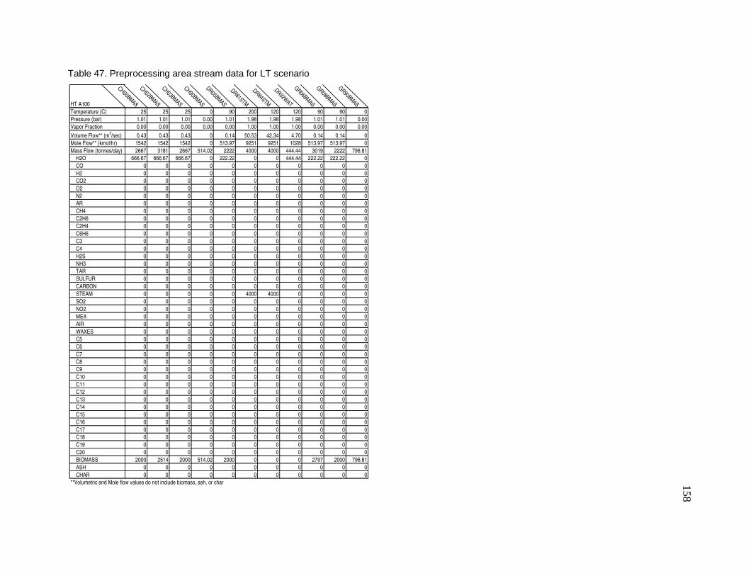
158 Table 47. Preprocessing area stream data for LT scenario

HT A100

CH00BMASCH02BMASCH03BMASCH90BMASDR05BMAS

.DR81STM

.DR84STM

.DR92WAT

GR06BMASGR08BMASGR90BMAS

Temperature (C) 25 25 25 0 90 200 120 120 90 90 0

Pressure (bar) 1.01 1.01 1.01 0.00 1.01 1.98 1.98 1.98 1.01 1.01 0.00

Vapor Fraction 0.00 0.00 0.00 0.00 0.00 1.00 1.00 1.00 0.00 0.00 0.00

Volume Flow** (m3/sec) 0.43 0.43 0.43 0 0.14 50.53 42.34 4.70 0.14 0.14 0

Mole Flow** (kmol/hr) 1542 1542 1542 0 513.97 9251 9251 1028 513.97 513.97 0

Mass Flow (tonnes/day) 2667 3181 2667 514.02 2222 4000 4000 444.44 3019 2222 796.81

H2O 666.67 666.67 666.67 0 222.22 0 0 444.44 222.22 222.22 0

CO 0 0 0 0 0 0 0 0 0 0 0

H2 0 0 0 0 0 0 0 0 0 0 0

CO2 0 0 0 0 0 0 0 0 0 0 0

O2 0 0 0 0 0 0 0 0 0 0 0

N2 0 0 0 0 0 0 0 0 0 0 0

AR 0 0 0 0 0 0 0 0 0 0 0

CH4 0 0 0 0 0 0 0 0 0 0 0

C2H6 0 0 0 0 0 0 0 0 0 0 0

C2H4 0 0 0 0 0 0 0 0 0 0 0

C6H6 0 0 0 0 0 0 0 0 0 0 0

C3 0 0 0 0 0 0 0 0 0 0 0

C4 0 0 0 0 0 0 0 0 0 0 0

H2S 0 0 0 0 0 0 0 0 0 0 0

NH3 0 0 0 0 0 0 0 0 0 0 0

TAR 0 0 0 0 0 0 0 0 0 0 0

SULFUR 0 0 0 0 0 0 0 0 0 0 0

CARBON 0 0 0 0 0 0 0 0 0 0 0

STEAM 0 0 0 0 0 4000 4000 0 0 0 0

SO2 0 0 0 0 0 0 0 0 0 0 0

NO2 0 0 0 0 0 0 0 0 0 0 0

MEA 0 0 0 0 0 0 0 0 0 0 0

AIR 0 0 0 0 0 0 0 0 0 0 0

WAXES 0 0 0 0 0 0 0 0 0 0 0

C5 0 0 0 0 0 0 0 0 0 0 0

C6 0 0 0 0 0 0 0 0 0 0 0

C7 0 0 0 0 0 0 0 0 0 0 0

C8 0 0 0 0 0 0 0 0 0 0 0

C9 0 0 0 0 0 0 0 0 0 0 0

C10 0 0 0 0 0 0 0 0 0 0 0

C11 0 0 0 0 0 0 0 0 0 0 0

C12 0 0 0 0 0 0 0 0 0 0 0

C13 0 0 0 0 0 0 0 0 0 0 0

C14 0 0 0 0 0 0 0 0 0 0 0

C15 0 0 0 0 0 0 0 0 0 0 0

C16 0 0 0 0 0 0 0 0 0 0 0

C17 0 0 0 0 0 0 0 0 0 0 0

C18 0 0 0 0 0 0 0 0 0 0 0

C19 0 0 0 0 0 0 0 0 0 0 0

C20 0 0 0 0 0 0 0 0 0 0 0

BIOMASS 2000 2514 2000 514.02 2000 0 0 0 2797 2000 796.81

ASH 0 0 0 0 0 0 0 0 0 0 0

CHAR 0 0 0 0 0 0 0 0 0 0 0

**Volumetric and Mole flow values do not include biomass, ash, or char

159 Table 48. Gasification area stream data for LT scenario

HT A200

CB52FLUE

CB61ASH

CB62ASHCY14SGASCY15CHARCY16CHARGS05SGASGS07SGASGS09CAIR

GS11BMASGS19CHARGS20SGAS

GS43CO2

GS46CO2GS52FLUE

GS81STM

GS84STM

GS90OX

GS91STM

Temperature (C) 1200 0 0 870 0 0 871 870 100 96 0 870 243 100 200 200 120 149 204

Pressure (bar) 1.00 1.00 1.00 27.57 27.57 27.55 28.00 27.58 1.01 1.01 27.55 27.55 28.00 27.58 1.00 1.98 1.98 22.00 22.00

Vapor Fraction 1.00 0.00 0.00 1.00 0.00 0.00 1.00 1.00 1.00 0.00 0.00 1.00 1.00 1.00 1.00 1.00 1.00 1.00 0.00

Volume Flow** (m3/sec) 69.99 0 0 2.38 0 0 4.69 4.76 16.89 0 0 4.76 0.07 0.05 22.48 50.53 42.34 0.32 0.01

Mole Flow** (kmol/hr) 2053 0 0 2470 0 0 4931 4939 1985 513.97 0 4939 170.42 161.90 2053 9251 9251 722.81 814.33

Mass Flow (tonnes/day) 1471 17.82 118.88 1477 95.38 12.09 3136 3145 1375 2222 214.95 2930 180.00 171.00 1471 4000 4000 561.66 352.09

H2O 27.16 0 0 206.71 0 0 413.42 413.42 0 222.22 0 413.42 0 0 27.16 0 0 0 352.09

CO 0 0 0 398.93 0 0 797.86 797.86 0 0 0 797.86 0 0 0 0 0 0 0

H2 0 0 0 23.87 0 0 47.75 47.75 0 0 0 47.75 0 0 0 0 0 0 0

CO2 239.52 0 0 713.66 0 0 1418 1427 0 0 0 1427 180.00 171.00 239.52 0 0 0 0

O2 148.99 0 0 0 0 0 0 0 320.19 0 0 0 0 0 148.99 0 0 528.66 0

N2 1055 0 0 0 0 0 0 0 1055 0 0 0 0 0 1055 0 0 0 0

AR 0 0 0 16.50 0 0 33.00 33.00 0 0 0 33.00 0 0 0 0 0 33.00 0

CH4 0 0 0 51.90 0 0 103.81 103.81 0 0 0 103.81 0 0 0 0 0 0 0

C2H6 0 0 0 10.91 0 0 21.82 21.82 0 0 0 21.82 0 0 0 0 0 0 0

C2H4 0 0 0 22.48 0 0 44.96 44.96 0 0 0 44.96 0 0 0 0 0 0 0

C6H6 0 0 0 2.05 0 0 4.10 4.10 0 0 0 4.10 0 0 0 0 0 0 0

C3 0 0 0 0 0 0 0 0 0 0 0 0 0 0 0 0 0 0 0

C4 0 0 0 0 0 0 0 0 0 0 0 0 0 0 0 0 0 0 0

H2S 0 0 0 2.25 0 0 4.51 4.51 0 0 0 4.51 0 0 0 0 0 0 0

NH3 0 0 0 9.54 0 0 19.09 19.09 0 0 0 19.09 0 0 0 0 0 0 0

TAR 0 0 0 5.29 0 0 10.57 10.57 0 0 0 10.57 0 0 0 0 0 0 0

SULFUR 0 0 0 0 0 0 0 0 0 0 0 0 0 0 0 0 0 0 0

CARBON 0 0 0 0 0 0 0 0 0 0 0 0 0 0 0 0 0 0 0

STEAM 0 0 0 0 0 0 0 0 0 0 0 0 0 0 0 4000 4000 0 0

SO2 0.30 0 0 0 0 0 0 0 0 0 0 0 0 0 0.30 0 0 0 0

NO2 0 0 0 0 0 0 0 0 0 0 0 0 0 0 0 0 0 0 0

MEA 0 0 0 0 0 0 0 0 0 0 0 0 0 0 0 0 0 0 0

AIR 0 0 0 0 0 0 0 0 0 0 0 0 0 0 0 0 0 0 0

WAXES 0 0 0 0 0 0 0 0 0 0 0 0 0 0 0 0 0 0 0

C5 0 0 0 0 0 0 0 0 0 0 0 0 0 0 0 0 0 0 0

C6 0 0 0 0 0 0 0 0 0 0 0 0 0 0 0 0 0 0 0

C7 0 0 0 0 0 0 0 0 0 0 0 0 0 0 0 0 0 0 0

C8 0 0 0 0 0 0 0 0 0 0 0 0 0 0 0 0 0 0 0

C9 0 0 0 0 0 0 0 0 0 0 0 0 0 0 0 0 0 0 0

C10 0 0 0 0 0 0 0 0 0 0 0 0 0 0 0 0 0 0 0

C11 0 0 0 0 0 0 0 0 0 0 0 0 0 0 0 0 0 0 0

C12 0 0 0 0 0 0 0 0 0 0 0 0 0 0 0 0 0 0 0

C13 0 0 0 0 0 0 0 0 0 0 0 0 0 0 0 0 0 0 0

C14 0 0 0 0 0 0 0 0 0 0 0 0 0 0 0 0 0 0 0

C15 0 0 0 0 0 0 0 0 0 0 0 0 0 0 0 0 0 0 0

C16 0 0 0 0 0 0 0 0 0 0 0 0 0 0 0 0 0 0 0

C17 0 0 0 0 0 0 0 0 0 0 0 0 0 0 0 0 0 0 0

C18 0 0 0 0 0 0 0 0 0 0 0 0 0 0 0 0 0 0 0

C19 0 0 0 0 0 0 0 0 0 0 0 0 0 0 0 0 0 0 0

C20 0 0 0 0 0 0 0 0 0 0 0 0 0 0 0 0 0 0 0

BIOMASS 0 0 0 0 0 0 0 0 0 2000 0 0 0 0 0 0 0 0 0

ASH 0.01 17.82 118.88 7.19 52.75 6.69 119.90 119.90 0 0 118.89 1.01 0 0 0.01 0 0 0 0

CHAR 0 0 0 5.81 42.63 5.40 96.87 96.87 0 0 96.06 0.81 0 0 0 0 0 0 0

**Volumetric and Mole flow values do not include biomass, ash, or char

160 Table 49. Syngas cleaning area stream data for LT scenario

HT A300

CL01H2O

CL02H2O

CL21SGAS

CL25ACG

CL25SGAS

CL25WAT

CL29SGAS

CL40CO2CL40SGAS

CL41CO2

CL43CO2

CL49SGAS

CL80H2O

CL80WAT

CL81WAT

CL83SUL

CL83WAT

CL84WAT

CL92AIR

CL95AIR

Temperature (C) 194 150 870 50 194 0 40 50 62 50 243 32 30 30 40 50 98 40 50 50

Pressure (bar) 27.55 27.55 27.55 3.45 27.55 27.55 26.86 3.45 22.89 3.45 28.00 22.89 27.57 27.57 26.86 2.07 27.55 27.55 2.07 2.07

Vapor Fraction 0.00 0.00 1.00 1.00 1.00 0.00 1.00 1.00 1.00 1.00 1.00 1.00 0.00 0.00 0.00 0.00 0.00 0.00 1.00 1.00

Volume Flow** (m3/sec) 0.08 0.08 4.76 3.28 2.03 0 0.98 3.21 2.40 2.84 0.07 1.50 0 0.01 0.02 0 0.07 0.07 0 0.10

Mole Flow** (kmol/hr) 13877 13877 4939 1538 5286 0 3638 1505 7066 1334 170.42 4869 346.93 1156 2804 5.56 13877 13877 0.45 27.74

Mass Flow (tonnes/day) 6000 6000 2930 1586 3078 1.82 2190 1560 2706 1380 180.00 2071 150.00 500.00 1388 3.10 6000 6000 0.35 22.89

H2O 6000 6000 413.42 22.78 563.42 0 3.78 20.50 30.18 20.50 0 0 150.00 500.00 1060 2.40 6000 6000 0 0.27

CO 0 0 797.86 3.07 797.86 0 782.59 0 1575 0 0 795.10 0 0 15.27 0 0 0 0 3.07

H2 0 0 47.75 0 47.75 0 47.68 0 168.38 0 0 120.71 0 0 0.07 0 0 0 0 0

CO2 0 0 1427 1539 1427 0 1164 1539 167.80 1359 180.00 559.11 0 0 263.09 0 0 0 0 0

O2 0 0 0 0 0 0 0 0 0 0 0 0 0 0 0 0 0 0 0.35 0

N2 0 0 0 0 0 0 0 0 0 0 0 0 0 0 0 0 0 0 0 0

AR 0 0 33.00 1.42 33.00 0 32.31 0 411.50 0 0 380.61 0 0 0.69 0 0 0 0 1.42

CH4 0 0 103.81 2.18 103.81 0 99.23 0 149.06 0 0 52.01 0 0 4.58 0 0 0 0 2.18

C2H6 0 0 21.82 1.11 21.82 0 16.07 0 28.49 0 0 13.55 0 0 5.75 0 0 0 0 1.11

C2H4 0 0 44.96 1.14 44.96 0 36.85 0 36.05 0 0 0.36 0 0 8.11 0 0 0 0 1.14

C6H6 0 0 4.10 0.15 4.10 0 3.11 0 39.50 0 0 36.54 0 0 0.98 0 0 0 0 0.15

C3 0 0 0 4.29 0 0 0 0 54.18 0 0 58.62 0 0 0 0 0 0 0 4.29

C4 0 0 0 6.73 0 0 0 0 34.31 0 0 41.73 0 0 0 0 0 0 0 6.73

H2S 0 0 4.51 2.48 4.51 0 2.64 0 0.13 0 0 0 0 0 1.87 0 0 0 0 1.73

NH3 0 0 19.09 0.42 19.09 0 1.73 0 1.52 0 0 0.28 0 0 17.36 0 0 0 0 0.42

TAR 0 0 10.57 0 10.57 0 0 0 0 0 0 0 0 0 10.57 0 0 0 0 0

SULFUR 0 0 0 0 0 0 0 0 0 0 0 0 0 0 0 0 0 0 0 0

CARBON 0 0 0 0 0 0 0 0 0 0 0 0 0 0 0 0 0 0 0 0

STEAM 0 0 0 0 0 0 0 0 0 0 0 0 0 0 0 0 0 0 0 0

SO2 0 0 0 0 0 0 0 0 0 0 0 0 0 0 0 0 0 0 0 0

NO2 0 0 0 0 0 0 0 0 0 0 0 0 0 0 0 0 0 0 0 0

MEA 0 0 0 0 0 0 0 0 0 0 0 0 0 0 0 0 0 0 0 0

AIR 0 0 0 0 0 0 0 0 0 0 0 0 0 0 0 0 0 0 0 0

WAXES 0 0 0 0 0 0 0 0 0 0 0 0 0 0 0 0 0 0 0 0

C5 0 0 0 0 0 0 0 0 2.21 0 0 2.21 0 0 0 0 0 0 0 0

C6 0 0 0 0 0 0 0 0 2.37 0 0 2.37 0 0 0 0 0 0 0 0

C7 0 0 0 0 0 0 0 0 1.11 0 0 1.11 0 0 0 0 0 0 0 0

C8 0 0 0 0 0 0 0 0 1.14 0 0 1.14 0 0 0 0 0 0 0 0

C9 0 0 0 0.07 0 0 0 0 1.08 0 0 1.15 0 0 0 0 0 0 0 0.07

C10 0 0 0 0.02 0 0 0 0 1.13 0 0 1.15 0 0 0 0 0 0 0 0.02

C11 0 0 0 0.03 0 0 0 0 0.50 0 0 0.54 0 0 0 0 0 0 0 0.03

C12 0 0 0 0.07 0 0 0 0 0.44 0 0 0.53 0 0 0 0 0 0 0 0.07

C13 0 0 0 0.10 0 0 0 0 0.34 0 0 0.51 0 0 0 0 0 0 0 0.10

C14 0 0 0 0.09 0 0 0 0 0.20 0 0 0.49 0 0 0 0 0 0 0 0.09

C15 0 0 0 0 0 0 0 0 0 0 0 0.46 0 0 0 0 0 0 0 0

C16 0 0 0 0.02 0 0 0 0 0.04 0 0 0.45 0 0 0 0 0 0 0 0.02

C17 0 0 0 0 0 0 0 0 0 0 0 0 0 0 0 0 0 0 0 0

C18 0 0 0 0 0 0 0 0 0 0 0 0 0 0 0 0 0 0 0 0

C19 0 0 0 0 0 0 0 0 0 0 0 0 0 0 0 0 0 0 0 0

C20 0 0 0 0 0 0 0 0 0 0 0 0 0 0 0 0 0 0 0 0

BIOMASS 0 0 0 0 0 0 0 0 0 0 0 0 0 0 0 0 0 0 0 0

ASH 0 0 1.01 0 0 1.01 0 0 0 0 0 0 0 0 0 0 0 0 0 0

CHAR 0 0 0.81 0 0 0.81 0 0 0 0 0 0 0 0 0 0 0 0 0 0

**Volumetric and Mole flow values do not include biomass, ash, or char

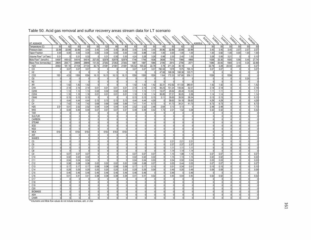
161 Table 50. Acid gas removal and sulfur recovery areas stream data for LT scenario

HT A300AGR

AG02MEARAG03MEARAG04MEARAG06MEARAG08MEALAG09MEALAG10MEALAG11MEAL

AG23ACG

AG24ACG

AG25ACGAG26SGASAG32SGASAG33SGASAG49SGAS A300SUL

SU25ACG

SU26SUL

SU40CO2

SU83SUL

SU92AIR

SU95AIR

Temperature (C) 50 62 50 93 50 123 80 80 93 50 50 40 50 62 32 50 50 50 50 50 50

Pressure (bar) 22.89 22.89 22.89 3.45 3.45 3.45 3.45 26.00 3.45 3.45 3.45 26.86 22.89 22.89 22.89 3.45 3.45 3.45 2.07 2.07 2.07

Vapor Fraction 0.00 0.00 0.00 0.00 0.00 0.00 0.00 0.00 1.00 0.88 1.00 1.00 0.93 1.00 1.00 1.00 0.82 1.00 0.00 1.00 1.00

Volume Flow** (m3/sec) 0.31 0 0.31 0.33 0 0.31 0.30 0.30 4.24 3.28 3.28 0.98 2.30 2.40 1.50 3.28 0.06 3.21 0 0 0.10

Mole Flow** (kmol/hr) 54067 449.42 54516 54516 207.83 52978 52978 52978 1746 1746 1538 3638 7515 7066 4869 1538 33.30 1505 5.56 0.45 27.74

Mass Flow (tonnes/day) 28640 208.71 28848 28848 101.05 27263 27263 27263 1687 1687 1586 2190 2915 2706 2071 1586 25.65 1560 3.10 0.35 22.89

H2O 20923 181.16 21104 21104 82.74 21081 21081 21081 105.52 105.52 22.78 3.78 211.34 30.18 0 22.78 2.28 20.50 2.40 0 0.27

CO 0 3.07 3.07 3.07 0 0 0 0 3.07 3.07 3.07 782.59 1578 1575 795.10 3.07 3.07 0 0 0 3.07

H2 0 0 0 0 0 0 0 0 0 0 0 47.68 168.38 168.38 120.71 0 0 0 0 0 0

CO2 1551 4.53 1556 1556 16.15 16.15 16.15 16.15 1556 1556 1539 1164 172.33 167.80 559.11 1539 0 1539 0 0 0

O2 0 0 0 0 0 0 0 0 0 0 0 0 0 0 0 0 0 0 0 0.35 0

N2 0 0 0 0 0 0 0 0 0 0 0 0 0 0 0 0 0 0 0 0 0

AR 0 1.42 1.42 1.42 0 0 0 0 1.42 1.42 1.42 32.31 412.92 411.50 380.61 1.42 1.42 0 0 0 1.42

CH4 0 2.19 2.19 2.19 0.01 0.01 0.01 0.01 2.19 2.19 2.18 99.23 151.24 149.06 52.01 2.18 2.18 0 0 0 2.18

C2H6 0 1.13 1.13 1.13 0.02 0.02 0.02 0.02 1.13 1.13 1.11 16.07 29.62 28.49 13.55 1.11 1.11 0 0 0 1.11

C2H4 0 1.16 1.16 1.16 0.01 0.01 0.01 0.01 1.16 1.16 1.14 36.85 37.21 36.05 0.36 1.14 1.14 0 0 0 1.14

C6H6 0 0.15 0.15 0.15 0 0 0 0 0.15 0.15 0.15 3.11 39.65 39.50 36.54 0.15 0.15 0 0 0 0.15

C3 0 4.44 4.44 4.44 0.15 0.15 0.15 0.15 4.44 4.44 4.29 0 58.62 54.18 58.62 4.29 4.29 0 0 0 4.29

C4 0 7.42 7.42 7.42 0.69 0.69 0.69 0.69 7.41 7.41 6.73 0 41.73 34.31 41.73 6.73 6.73 0 0 0 6.73

H2S 2.51 0.01 2.52 2.52 0.04 0.04 0.04 0.04 2.52 2.52 2.48 2.64 0.13 0.13 0 2.48 2.48 0 0 0 1.73

NH3 0 0.49 0.49 0.49 0.07 0.07 0.07 0.07 0.49 0.49 0.42 1.73 2.01 1.52 0.28 0.42 0.42 0 0 0 0.42

TAR 0 0 0 0 0 0 0 0 0 0 0 0 0 0 0 0 0 0 0 0 0

SULFUR 0 0 0 0 0 0 0 0 0 0 0 0 0 0 0 0 0 0 0 0 0

CARBON 0 0 0 0 0 0 0 0 0 0 0 0 0 0 0 0 0 0 0 0 0

STEAM 0 0 0 0 0 0 0 0 0 0 0 0 0 0 0 0 0 0 0 0 0

SO2 0 0 0 0 0 0 0 0 0 0 0 0 0 0 0 0 0 0 0 0 0

NO2 0 0 0 0 0 0 0 0 0 0 0 0 0 0 0 0 0 0 0 0 0

MEA 6163 0 6163 6163 0 6163 6163 6163 0 0 0 0 0 0 0 0 0 0 0 0 0

AIR 0 0 0 0 0 0 0 0 0 0 0 0 0 0 0 0 0 0 0 0 0

WAXES 0 0 0 0 0 0 0 0 0 0 0 0 0 0 0 0 0 0 0 0 0

C5 0 0 0 0 0 0 0 0 0 0 0 0 2.21 2.21 2.21 0 0 0 0 0 0

C6 0 0 0 0 0 0 0 0 0 0 0 0 2.37 2.37 2.37 0 0 0 0 0 0

C7 0 0 0 0 0 0 0 0 0 0 0 0 1.11 1.11 1.11 0 0 0 0 0 0

C8 0 0 0 0 0 0 0 0 0 0 0 0 1.14 1.14 1.14 0 0 0 0 0 0

C9 0 0.07 0.07 0.07 0 0 0 0 0.07 0.07 0.07 0 1.15 1.08 1.15 0.07 0.07 0 0 0 0.07

C10 0 0.02 0.02 0.02 0 0 0 0 0.02 0.02 0.02 0 1.15 1.13 1.15 0.02 0.02 0 0 0 0.02

C11 0 0.04 0.04 0.04 0 0 0 0 0.04 0.04 0.03 0 0.54 0.50 0.54 0.03 0.03 0 0 0 0.03

C12 0 0.08 0.08 0.08 0.02 0.02 0.02 0.02 0.08 0.08 0.07 0 0.53 0.44 0.53 0.07 0.07 0 0 0 0.07

C13 0 0.17 0.17 0.17 0.08 0.08 0.08 0.08 0.17 0.17 0.10 0 0.51 0.34 0.51 0.10 0.10 0 0 0 0.10

C14 0 0.29 0.29 0.29 0.20 0.20 0.20 0.20 0.29 0.29 0.09 0 0.49 0.20 0.49 0.09 0.09 0 0 0 0.09

C15 0 0.46 0.46 0.46 0.46 0.46 0.46 0.46 0.46 0.46 0 0 0.46 0 0.46 0 0 0 0 0 0

C16 0 0.41 0.41 0.41 0.38 0.38 0.38 0.38 0.41 0.41 0.02 0 0.45 0.04 0.45 0.02 0.02 0 0 0 0.02

C17 0 0 0 0 0 0 0 0 0 0 0 0 0 0 0 0 0 0 0 0 0

C18 0 0 0 0 0 0 0 0 0 0 0 0 0 0 0 0 0 0 0 0 0

C19 0 0 0 0 0 0 0 0 0 0 0 0 0 0 0 0 0 0 0 0 0

C20 0 0 0 0 0 0 0 0 0 0 0 0 0 0 0 0 0 0 0 0 0

BIOMASS 0 0 0 0 0 0 0 0 0 0 0 0 0 0 0 0 0 0 0 0 0

ASH 0 0 0 0 0 0 0 0 0 0 0 0 0 0 0 0 0 0 0 0 0

CHAR 0 0 0 0 0 0 0 0 0 0 0 0 0 0 0 0 0 0 0 0 0

**Volumetric and Mole flow values do not include biomass, ash, or char

162 Table 51. Fuel synthesis area stream data for LT scenario

HT A400

FS34SGAS

FS35SGAS

FS36SGAS

FS37SGAS

FS40SGAS

FS41GAS

FS50SGAS

FS51FT

FS52FT

FS53SGAS

FS54FT

FS55SGAS

FS56FT

FS56SGAS

FS57SGAS

FS58SGAS

FS59SGAS

FS60WAT

FS90HYD

Temperature (C) 62 78 200 200 60 235 200 200 35 32 35 32 35 32 32 41 200 35 60

Pressure (bar) 22.89 26.50 25.12 25.12 1.01 25.00 24.96 22.89 22.89 22.89 22.89 22.89 22.89 22.89 22.89 25.30 24.96 22.89 1.01

Vapor Fraction 1.00 1.00 1.00 1.00 0.88 1.00 1.00 1.00 0.72 1.00 0.00 1.00 0.00 1.00 1.00 1.00 1.00 0.00 1.00

Volume Flow** (m3/sec) 2.40 2.18 4.44 0.07 0.65 0.05 5.02 4.39 2.08 2.02 0.01 1.50 0.01 0.12 0.41 0.38 0.58 0.01 0.53

Mole Flow** (kmol/hr) 7066 7066 10153 166.97 97.01 97.01 11399 9268 9268 6579 70.21 4869 69.40 394.75 1316 1316 1316 2619 69.96

Mass Flow (tonnes/day) 2706 2706 3705 60.93 57.55 57.55 4261 4261 4261 2798 330.77 2071 330.42 167.90 559.66 559.66 559.66 1132 3.38

H2O 30.18 30.18 671.91 11.05 11.05 11.05 671.91 1133 1133 0 0.43 0 0.09 0 0 0 0 1132 0

CO 1575 1575 1576 25.92 25.92 25.92 1791 1074 1074 1074 0 795.10 0 64.47 214.89 214.89 214.89 0 0

H2 168.38 168.38 242.13 3.98 0.60 0.60 271.37 163.12 163.12 163.12 0 120.71 0 9.79 32.62 32.62 32.62 0 3.38

CO2 167.80 167.80 604.44 9.94 9.94 9.94 755.55 755.55 755.55 755.55 0 559.11 0 45.33 151.11 151.11 151.11 0 0

O2 0 0 0 0 0 0 0 0 0 0 0 0 0 0 0 0 0 0 0

N2 0 0 0 0 0 0 0 0 0 0 0 0 0 0 0 0 0 0 0

AR 411.50 411.50 411.50 6.77 6.77 6.77 514.36 514.36 514.36 514.34 0 380.61 0 30.86 102.87 102.87 102.87 0 0

CH4 149.06 149.06 52.13 0.86 0.86 0.86 66.19 70.29 70.29 70.29 0 52.01 0 4.22 14.06 14.06 14.06 0 0

C2H6 28.49 28.49 7.72 0.13 0.13 0.13 11.38 18.30 18.30 18.30 0 13.55 0 1.10 3.66 3.66 3.66 0 0

C2H4 36.05 36.05 0.39 0.01 0.01 0.01 0.49 0.49 0.49 0.49 0 0.36 0 0.03 0.10 0.10 0.10 0 0

C6H6 39.50 39.50 39.50 0.65 0.65 0.65 49.38 49.38 49.38 49.38 0 36.54 0 2.96 9.88 9.88 9.88 0 0

C3 54.18 54.18 54.18 0.89 0.89 0.89 70.02 79.16 79.16 79.22 0 58.62 0 4.75 15.84 15.84 15.84 0 0

C4 34.31 34.31 34.31 0.56 0.56 0.56 45.59 56.43 56.43 56.40 0 41.73 0 3.38 11.28 11.28 11.28 0 0

H2S 0.13 0.13 0.01 0 0 0 0.01 0.01 0.01 0.01 0 0 0 0 0 0 0 0 0

NH3 1.52 1.52 0.30 0 0 0 0.38 0.38 0.38 0.38 0 0.28 0 0.02 0.08 0.08 0.08 0 0

TAR 0 0 0 0 0 0 0 0 0 0 0 0 0 0 0 0 0 0 0

SULFUR 0 0 0 0 0 0 0 0 0 0 0 0 0 0 0 0 0 0 0

CARBON 0 0 0 0 0 0 0 0 0 0 0 0 0 0 0 0 0 0 0

STEAM 0 0 0 0 0 0 0 0 0 0 0 0 0 0 0 0 0 0 0

SO2 0 0 0 0 0 0 0 0 0 0 0 0 0 0 0 0 0 0 0

NO2 0 0 0 0 0 0 0 0 0 0 0 0 0 0 0 0 0 0 0

MEA 0 0 0 0 0 0 0 0 0 0 0 0 0 0 0 0 0 0 0

AIR 0 0 0 0 0 0 0 0 0 0 0 0 0 0 0 0 0 0 0

WAXES 0 0 0 0 0 0 0 131.46 131.46 0 131.46 0 131.46 0 0 0 0 0 0

C5 2.21 2.21 2.21 0.04 0.04 0.04 2.80 14.91 14.91 2.98 11.92 2.21 11.92 0.18 0.60 0.60 0.60 0 0

C6 2.37 2.37 2.37 0.04 0.04 0.04 3.01 16.02 16.02 3.20 12.82 2.37 12.82 0.19 0.64 0.64 0.64 0 0

C7 1.11 1.11 1.11 0.02 0.02 0.02 1.41 15.03 15.03 1.50 13.53 1.11 13.53 0.09 0.30 0.30 0.30 0 0

C8 1.14 1.14 1.14 0.02 0.02 0.02 1.45 15.42 15.42 1.54 13.88 1.14 13.88 0.09 0.31 0.31 0.31 0 0

C9 1.08 1.08 1.08 0.02 0.02 0.02 1.39 15.50 15.50 1.55 13.95 1.15 13.95 0.09 0.31 0.31 0.31 0 0

C10 1.13 1.13 1.13 0.02 0.02 0.02 1.44 15.54 15.54 1.55 13.98 1.15 13.98 0.09 0.31 0.31 0.31 0 0

C11 0.50 0.50 0.50 0.01 0.01 0.01 0.65 14.59 14.59 0.73 13.86 0.54 13.86 0.04 0.15 0.15 0.15 0 0

C12 0.44 0.44 0.44 0.01 0.01 0.01 0.59 14.26 14.26 0.71 13.54 0.53 13.54 0.04 0.14 0.14 0.14 0 0

C13 0.34 0.34 0.34 0.01 0.01 0.01 0.47 13.79 13.79 0.69 13.10 0.51 13.10 0.04 0.14 0.14 0.14 0 0

C14 0.20 0.20 0.20 0 0 0 0.34 13.23 13.23 0.66 12.57 0.49 12.57 0.04 0.13 0.13 0.13 0 0

C15 0 0 0 0 0 0 0.13 12.55 12.55 0.63 11.93 0.46 11.93 0.04 0.13 0.13 0.13 0 0

C16 0.04 0.04 0.04 0 0 0 0.16 12.08 12.08 0.60 11.48 0.45 11.48 0.04 0.12 0.12 0.12 0 0

C17 0 0 0 0 0 0 0 11.39 11.39 0 11.39 0 11.39 0 0 0 0 0 0

C18 0 0 0 0 0 0 0 10.85 10.85 0 10.85 0 10.85 0 0 0 0 0 0

C19 0 0 0 0 0 0 0 10.31 10.31 0 10.31 0 10.31 0 0 0 0 0 0

C20 0 0 0 0 0 0 0 9.76 9.76 0 9.76 0 9.76 0 0 0 0 0 0

BIOMASS 0 0 0 0 0 0 0 0 0 0 0 0 0 0 0 0 0 0 0

ASH 0 0 0 0 0 0 0 0 0 0 0 0 0 0 0 0 0 0 0

CHAR 0 0 0 0 0 0 0 0 0 0 0 0 0 0 0 0 0 0 0

**Volumetric and Mole flow values do not include biomass, ash, or char

163 Table 52. Syngas conditioning area stream data for LT scenario

HT A400COND

CD35SGAS

CD36SGAS

CD37SGAS

CD38SGAS

CD39SGAS

CD40SGAS

CD41SGAS

CD42SGAS

CD44SGAS

CD45SGAS

CD80STM

CD81STM

CD99CONT

Temperature (C) 78 150 150 870 870 300 300 474 363 200 300 870 150

Pressure (bar) 26.50 26.50 26.50 26.50 25.81 25.81 25.81 25.12 25.12 25.12 25.00 27.00 26.50

Vapor Fraction 1.00 1.00 1.00 1.00 1.00 1.00 1.00 1.00 1.00 1.00 1.00 1.00 1.00

Volume Flow** (m3/sec) 2.18 2.64 2.64 7.08 10.44 5.24 1.83 2.46 5.98 4.44 1.15 2.26 0

Mole Flow** (kmol/hr) 7066 7066 7063 7063 10153 10153 3554 3554 10153 10153 2313 2313 3.12

Mass Flow (tonnes/day) 2706 2706 2705 2705 3705 3705 1297 1297 3705 3705 1000 1000 1.34

H2O 30.18 30.18 30.18 30.18 850.65 850.65 297.73 118.99 671.91 671.91 1000 1000 0

CO 1575 1575 1575 1575 1854 1854 648.81 370.91 1576 1576 0 0 0

H2 168.38 168.38 168.38 168.38 222.13 222.13 77.75 97.75 242.13 242.13 0 0 0

CO2 167.80 167.80 167.80 167.80 167.80 167.80 58.73 495.37 604.44 604.44 0 0 0

O2 0 0 0 0 0 0 0 0 0 0 0 0 0

N2 0 0 0 0 0 0 0 0 0 0 0 0 0

AR 411.50 411.50 411.50 411.50 411.50 411.50 144.02 144.02 411.50 411.50 0 0 0

CH4 149.06 149.06 149.06 149.06 52.13 52.13 18.25 18.25 52.13 52.13 0 0 0

C2H6 28.49 28.49 28.49 28.49 7.72 7.72 2.70 2.70 7.72 7.72 0 0 0

C2H4 36.05 36.05 36.05 36.05 0.39 0.39 0.14 0.14 0.39 0.39 0 0 0

C6H6 39.50 39.50 39.50 39.50 39.50 39.50 13.83 13.83 39.50 39.50 0 0 0

C3 54.18 54.18 54.18 54.18 54.18 54.18 18.96 18.96 54.18 54.18 0 0 0

C4 34.31 34.31 34.31 34.31 34.31 34.31 12.01 12.01 34.31 34.31 0 0 0

H2S 0.13 0.13 0.01 0.01 0.01 0.01 0 0 0.01 0.01 0 0 0.12

NH3 1.52 1.52 0.30 0.30 0.30 0.30 0.11 0.11 0.30 0.30 0 0 1.21

TAR 0 0 0 0 0 0 0 0 0 0 0 0 0

SULFUR 0 0 0 0 0 0 0 0 0 0 0 0 0

CARBON 0 0 0 0 0 0 0 0 0 0 0 0 0

STEAM 0 0 0 0 0 0 0 0 0 0 0 0 0

SO2 0 0 0 0 0 0 0 0 0 0 0 0 0

NO2 0 0 0 0 0 0 0 0 0 0 0 0 0

MEA 0 0 0 0 0 0 0 0 0 0 0 0 0

AIR 0 0 0 0 0 0 0 0 0 0 0 0 0

WAXES 0 0 0 0 0 0 0 0 0 0 0 0 0

C5 2.21 2.21 2.21 2.21 2.21 2.21 0.77 0.77 2.21 2.21 0 0 0

C6 2.37 2.37 2.37 2.37 2.37 2.37 0.83 0.83 2.37 2.37 0 0 0

C7 1.11 1.11 1.11 1.11 1.11 1.11 0.39 0.39 1.11 1.11 0 0 0

C8 1.14 1.14 1.14 1.14 1.14 1.14 0.40 0.40 1.14 1.14 0 0 0

C9 1.08 1.08 1.08 1.08 1.08 1.08 0.38 0.38 1.08 1.08 0 0 0

C10 1.13 1.13 1.13 1.13 1.13 1.13 0.40 0.40 1.13 1.13 0 0 0

C11 0.50 0.50 0.50 0.50 0.50 0.50 0.18 0.18 0.50 0.50 0 0 0

C12 0.44 0.44 0.44 0.44 0.44 0.44 0.16 0.16 0.44 0.44 0 0 0

C13 0.34 0.34 0.34 0.34 0.34 0.34 0.12 0.12 0.34 0.34 0 0 0

C14 0.20 0.20 0.20 0.20 0.20 0.20 0.07 0.07 0.20 0.20 0 0 0

C15 0 0 0 0 0 0 0 0 0 0 0 0 0

C16 0.04 0.04 0.04 0.04 0.04 0.04 0.01 0.01 0.04 0.04 0 0 0

C17 0 0 0 0 0 0 0 0 0 0 0 0 0

C18 0 0 0 0 0 0 0 0 0 0 0 0 0

C19 0 0 0 0 0 0 0 0 0 0 0 0 0

C20 0 0 0 0 0 0 0 0 0 0 0 0 0

BIOMASS 0 0 0 0 0 0 0 0 0 0 0 0 0

ASH 0 0 0 0 0 0 0 0 0 0 0 0 0

CHAR 0 0 0 0 0 0 0 0 0 0 0 0 0

**Volumetric and Mole flow values do not include biomass, ash, or char

164 Table 53. Hydroprocessing, power generation, and air separation areas stream data for LT scenario

HT A500

HY56FTHY65FGASHY70GASOHY71GASO

HY80DIESHY81DIES

HY90HYD A600

421

602

615

680

CW2

CWREC

HPW1

HPSTM A700

AIR-1A

AIR-A

AIR-L

N2-OUT

O2LPC

O2-OUT

O2-OUT2

Temperature (C) 35 50 50 50 50 50 60 32 1161 344 30 85 23 170 393 -170 32 20 16 35 16 55

Pressure (bar) 22.89 22.89 22.89 22.89 22.89 22.89 1.01 22.89 1.00 1.00 1.01 7.91 0.02 7.91 173.38 6.20 1.01 6.30 1.10 23.08 1.10 27.00

Vapor Fraction 0.00 1.00 0.00 0.00 0.00 0.00 1.00 1.00 1.00 1.00 1.00 0.00 0.89 0.00 1.00 1.00 1.00 1.00 1.00 1.00 1.00 1.00

Volume Flow** (m3/sec) 0.01 0.02 0 0 0 0 0.53 0.12 94.88 40.84 17.42 0.01 442.16 0 0.03 1.06 23.17 3.58 15.73 0.22 4.45 0.21

Mole Flow** (kmol/hr) 69.40 57.67 31.78 31.78 37.88 37.88 69.96 394.75 2863 2863 2522 1709 1709 1709 1709 3162 3328 3328 2594 734.20 734.20 734.20

Mass Flow (tonnes/day) 330.42 40.83 87.12 87.12 205.86 205.86 3.38 167.90 1955 1955 1746 740.10 740.10 740.10 740.10 2198 2313 2313 1744 569.18 569.18 569.18

H2O 0.09 0 0 0 0 0 0 0 189.23 189.23 0 740.10 740.10 740.10 740.10 0 0 0 0 0 0 0

CO 0 0 0 0 0 0 0 64.47 0 0 0 0 0 0 0 0 0 0 0 0 0 0

H2 0 0 0 0 0 0 3.38 9.79 0 0 0 0 0 0 0 0 0 0 0 0 0 0

CO2 0 0 0 0 0 0 0 45.33 318.35 318.35 0 0 0 0 0 0 0 0 0 0 0 0

O2 0 0 0 0 0 0 0 0 80.99 80.99 410.78 0 0 0 0 508.87 535.65 535.65 0 535.65 535.65 535.65

N2 0 0 0 0 0 0 0 0 1336 1336 1336 0 0 0 0 1661 1748 1748 1744 3.91 3.91 3.91

AR 0 0 0 0 0 0 0 30.86 30.86 30.86 0 0 0 0 0 28.22 29.71 29.71 0.10 29.61 29.61 29.61

CH4 0 11.56 0 0 0 0 0 4.22 0 0 0 0 0 0 0 0 0 0 0 0 0 0

C2H6 0 0 0 0 0 0 0 1.10 0 0 0 0 0 0 0 0 0 0 0 0 0 0

C2H4 0 0 0 0 0 0 0 0.03 0 0 0 0 0 0 0 0 0 0 0 0 0 0

C6H6 0 0 0 0 0 0 0 2.96 0 0 0 0 0 0 0 0 0 0 0 0 0 0

C3 0 29.27 0 0 0 0 0 4.75 0 0 0 0 0 0 0 0 0 0 0 0 0 0

C4 0 0 0 0 0 0 0 3.38 0 0 0 0 0 0 0 0 0 0 0 0 0 0

H2S 0 0 0 0 0 0 0 0 0 0 0 0 0 0 0 0 0 0 0 0 0 0

NH3 0 0 0 0 0 0 0 0.02 0 0 0 0 0 0 0 0 0 0 0 0 0 0

TAR 0 0 0 0 0 0 0 0 0 0 0 0 0 0 0 0 0 0 0 0 0 0

SULFUR 0 0 0 0 0 0 0 0 0 0 0 0 0 0 0 0 0 0 0 0 0 0

CARBON 0 0 0 0 0 0 0 0 0 0 0 0 0 0 0 0 0 0 0 0 0 0

STEAM 0 0 0 0 0 0 0 0 0 0 0 0 0 0 0 0 0 0 0 0 0 0

SO2 0 0 0 0 0 0 0 0 0 0 0 0 0 0 0 0 0 0 0 0 0 0

NO2 0 0 0 0 0 0 0 0 0.06 0.06 0 0 0 0 0 0 0 0 0 0 0 0

MEA 0 0 0 0 0 0 0 0 0 0 0 0 0 0 0 0 0 0 0 0 0 0

AIR 0 0 0 0 0 0 0 0 0 0 0 0 0 0 0 0 0 0 0 0 0 0

WAXES 131.46 0 0 0 0 0 0 0 0 0 0 0 0 0 0 0 0 0 0 0 0 0

C5 11.92 0 0 0 0 0 0 0.18 0 0 0 0 0 0 0 0 0 0 0 0 0 0

C6 12.82 0 0 0 0 0 0 0.19 0 0 0 0 0 0 0 0 0 0 0 0 0 0

C7 13.53 0 0 0 0 0 0 0.09 0 0 0 0 0 0 0 0 0 0 0 0 0 0

C8 13.88 0 87.12 87.12 0 0 0 0.09 0 0 0 0 0 0 0 0 0 0 0 0 0 0

C9 13.95 0 0 0 0 0 0 0.09 0 0 0 0 0 0 0 0 0 0 0 0 0 0

C10 13.98 0 0 0 0 0 0 0.09 0 0 0 0 0 0 0 0 0 0 0 0 0 0

C11 13.86 0 0 0 0 0 0 0.04 0 0 0 0 0 0 0 0 0 0 0 0 0 0

C12 13.54 0 0 0 0 0 0 0.04 0 0 0 0 0 0 0 0 0 0 0 0 0 0

C13 13.10 0 0 0 0 0 0 0.04 0 0 0 0 0 0 0 0 0 0 0 0 0 0

C14 12.57 0 0 0 0 0 0 0.04 0 0 0 0 0 0 0 0 0 0 0 0 0 0

C15 11.93 0 0 0 0 0 0 0.04 0 0 0 0 0 0 0 0 0 0 0 0 0 0

C16 11.48 0 0 0 205.86 205.86 0 0.04 0 0 0 0 0 0 0 0 0 0 0 0 0 0

C17 11.39 0 0 0 0 0 0 0 0 0 0 0 0 0 0 0 0 0 0 0 0 0

C18 10.85 0 0 0 0 0 0 0 0 0 0 0 0 0 0 0 0 0 0 0 0 0

C19 10.31 0 0 0 0 0 0 0 0 0 0 0 0 0 0 0 0 0 0 0 0 0

C20 9.76 0 0 0 0 0 0 0 0 0 0 0 0 0 0 0 0 0 0 0 0 0

BIOMASS 0 0 0 0 0 0 0 0 0 0 0 0 0 0 0 0 0 0 0 0 0 0

ASH 0 0 0 0 0 0 0 0 0 0 0 0 0 0 0 0 0 0 0 0 0 0

CHAR 0 0 0 0 0 0 0 0 0 0 0 0 0 0 0 0 0 0 0 0 0 0

**Volumetric and Mole flow values do not include biomass, ash, or char