No 233 – April 2016

Technology Adoption and Risk Exposure among Smallholder Farmers: Panel Data Evidence from Tanzania

and Uganda

Adamon N. Mukasa

Editorial Committee

Shimeles, Abebe (Chair) Anyanwu, John C. Faye, Issa Ngaruko, Floribert Simpasa, Anthony Salami, Adeleke O. Verdier-Chouchane, Audrey

Coordinator

Salami, Adeleke O.

Rights and Permissions

All rights reserved.

The text and data in this publication may be

reproduced as long as the source is cited.

Reproduction for commercial purposes is

forbidden.

The Working Paper Series (WPS) is produced by the

Development Research Department of the African

Development Bank. The WPS disseminates the

findings of work in progress, preliminary research

results, and development experience and lessons,

to encourage the exchange of ideas and innovative

thinking among researchers, development

practitioners, policy makers, and donors. The

findings, interpretations, and conclusions

expressed in the Bank’s WPS are entirely those of

the author(s) and do not necessarily represent the

view of the African Development Bank, its Board of

Directors, or the countries they represent.

Copyright © 2016

African Development Bank

Immeuble du Centre de Commerce International d'

Abidjan (CCIA)

01 BP 1387, Abidjan 01

Côte d'Ivoire

E-mail: afdb@afdb.org

Working Papers are available online at

http:/www.afdb.org/

Correct citation: Mukasa, Adamon N. (2016), Technology Adoption and Risk Exposure among Smallholder Farmers: Panel Data Evidence from Tanzania and Uganda, Working Paper Series N° 233 African Development Bank, Abidjan, Côte d’Ivoire.

Technology Adoption and Risk Exposure among Smallholder Farmers: Panel Data Evidence from Tanzania

and Uganda

Adamon N. Mukasa1

1 Adamon N. Mukasa is a consultant at the African Development Bank, Abidjan, Côte d’Ivoire

(a.ndungu@afdb.org). This paper was conceptualized and finalized while the author was a consultant

under the “Structural Transformation of African Agriculture and Rural Spaces – STAARS” project. The author also acknowledges funding support from the African Development Bank Group under the STAARS project. The author would like to thank all participants to the STAARS inaugural conference held on December 4-5, 2015 in Addis Ababa, Ethiopia for their helpful comments. Special thanks to colleagues at the Development Research Department of the African Development Bank for their comments and suggestions that substantially improved the paper quality. The usual disclaimer applies.

AFRICAN DEVELOPMENT BANK GROUP

Working Paper No. 233

April 2016

Office of the Chief Economist

Abstract

This paper investigates the empirical

linkages between production risk and

technology adoption decisions among

agricultural farmers in Tanzania and

Uganda using a balanced household

panel dataset from the World Bank’s

LSMS-ISA project. Applying a moment-

based approach and a Mundlak-

Chamberlain IV fixed effects model to

control for endogeneity and unobserved

heterogeneity, I find that the first four

moments of production significantly

explain changes in the probability of

adopting chemical fertilizer, improved

seeds, and pesticides. While the use of

these modern inputs is found to be risk-

decreasing, estimates suggest that the

higher their purchasing costs, the greater

the cost of farmers’ private risk bearing.

Under the assumption of a moderate risk

aversion, the risk premium amounts to

12.7% and 30.5% of the expected

production revenues respectively in

Tanzania and Uganda, largely explained

by production volatility and downside

risk aversion. This underscores the need

to account for farmers’ preferences

towards higher order moments when

designing technology adoption policies.

Key words: Production risk, technology adoption, LSMS, Tanzania, Uganda

5

1. INTRODUCTION

In most developing countries, increasing agricultural productivity is the overarching goal of

policy makers and their development partners. Especially for sub-Saharan African (SSA)

countries where half of the population lives in poverty, technological changes in the

agricultural sector are often considered as one of the key pathways for fighting food insecurity,

spurring economic growth, overcoming extreme poverty, and improving populations’

wellbeing. Indeed, in many of these countries, the majority of households still live in rural areas

and depend on agricultural activities as their main employment and earning sources. In

Tanzania and Uganda for example where around 80% of the population lives in rural areas, the

agricultural sector contributes at least 25% of the Gross Domestic Product, provides about 45%

of earning sources, and employs over 65% of the total labor force of the country (World Bank,

2015).

Notwithstanding the acclaimed contribution of agriculture to economic growth, land

productivity remains distressfully low in the majority, if not all, SSA countries, thereby

jeopardizing the food security of their population and increasing the risks of poverty traps of

the most vulnerable, particularly women and children. Among the culprits, we often find land

degradation due to nutrient depletion and soil erosion (Juma et al, 2009), population pressure,

extreme temperature, inadequate rainfall, and inappropriately applied agricultural technologies

or mismatched agricultural policies (Duflo et al,2008).

As a result, SSA governments and their development partners dedicated considerable resources

to enhance environmental conditions, stimulate economic growth, and increase agricultural

productivity. Various agricultural extension services such as the National Agricultural

Advisory Services (NAADS) in Uganda, soil and water conservation programs in Kenya, or

agricultural marketing and irrigation programs in Tanzania have thus been geared towards

improving agricultural production and productivity and sustaining farmers’ wellbeing and

livelihoods. In those programs, a clear emphasis has been put on the adoption of modern

agricultural technologies such as high-yielding varieties (HYV), improved seeds, inorganic

fertilizer, or other agro-chemicals which are expected to increase agricultural productivity,

stimulate the transition from subsistence farming to agro-industry, lower per unit production

costs, increase incomes of technology adopters, and subsequently enhance farmers’ wellbeing

(de Janvry and Sadoulet, 2001; Mendola, 2007; Kijima et al, 2008; Kassie et al, 2011).

Although the adoption of these modern technologies is considered as an important tool to fight

poverty in many developing countries (Bandiera and Rasul, 2006; Croppenstedt et al, 2003),

its impact is however hampered in many SSA countries by low adoption rates. For example, in

2012, SSA farmers applied on average only 12.3kg per hectare of arable land compared to the

world average of 141.3kg (World Bank, 2015). There are various theoretical and empirical

explanations for these paltry application rates. They include lack of sufficient resources to

purchase modern inputs, and their relatively low profitability (Duflo et al, 2008), limited access

to credit and labor constraints (Croppenstedt et al, 2003; Ndjeunga and Bantilan, 2005; Moser

6

and Barrett, 2006; Langyintuo et al, 2010), high transaction and transportation costs (Minten

et al, 2013); insufficient knowledge about new agricultural technologies or their availability

(Conley and Udry, 2010; Krishnan and Patnam, 2014), and high production, climatic, or price

risks (Koundouri et al, 2006; Juma et al, 2009; Giné and Yang, 2009; Dercon and

Christiaensen, 2011).

In this paper, I analyze the role of risk exposure in farm production decisions, especially in the

uptake of new and/or modern technologies. Interest in risks stems from the empirical evidence

that most farmers are risk averse (Binswanger, 1981; Antle, 1983, 1987; Saha et al, 1994; Kim

and Chavas, 2003). Risk-averse farmers will often be reluctant to adopt new technologies and

may consistently apply low productive technologies with low profitability which may therefore

thrust them into permanent food insecurity conditions (Rosenzweig and Binswanger 1993;

Dercon and Christiaensen, 2011). Furthermore, the extra caution due to risk aversion attitude

and the lack of both ex ante and ex post coping mechanisms such as formal and informal credit

and insurance schemes may prevent farmers from undertaking profitable capital investments

and earning sufficient revenues to move permanently out of poverty.

A number of authors have documented the role of production risks in agriculture and their

effects on adoption of modern technologies (Lamb, 2003; Koundouri et al, 2006; Groom et al,

2008; Juma et al, 2009; Kassie et al, 2011; Holden, 2015). However, despite the profusion of

studies, there are often mixed conclusions regarding the identification and relative importance

of risk factors in driving technology adoption decisions. This may be attributed not only to

structural differences of agriculture across various regions of the world, but also to the complex

dynamics of the technology adoption process (Moser and Barrett, 2006) and to important

shortcomings in the methodological approaches of prior studies. First, with notable exceptions

of Lamb (2003) and Dercon and Christiaensen (2011), previous studies used cross-sectional

data and econometric methods that do not account for farmers’ unobserved heterogeneity

which, if not controlled for, may lead to potentially inconsistent and biased parameter

estimates. Also, existing adoption studies have focused on either a single new technology

(improved water and irrigation system, modern fertilizer, or improved seeds) or a set of modern

technologies treated as a unique bundle (Dorfman, 1996). However, farmers often combine

different new technologies in order to maximize the potential benefits of each of them. In other

words, the adoption decision may be described more like a multivariate adoption than a

univariate process.

In this paper, I address these issues by using farm- and plot-level panel datasets and extend the

moment-based approach of Antle (1983, 1987), derive production risk variables and control

for unobserved heterogeneity. Moreover, to address potential endogeneity problems during the

estimation, a two-stage Instrument Variables (IV) approach is employed. Accordingly, the

possibility of interdependent and simultaneous technology adoption decisions is also accounted

for by applying a multivariate approach to the modelling of adoption decisions (Dorfman,

1996; Teklewold et al, 2013). The empirical approach is applied to smallholder farmers in

Tanzania and Uganda, two SSA countries where panel household datasets from the Living

Standards Measurement Study – Integrated Surveys on Agriculture (LSMS-ISA) are currently

7

the longest. Findings from these countries may also provide useful insights to the understanding

of technology adoption in other SSA countries with relatively similar technology adoption

profiles.

The remainder of the paper is organized as follows. Section 2 presents the conceptual

framework used to analyze farmers’ adoption decisions in the presence of production risks.

Section 3 details the empirical approach and discusses the main econometric issues. Data

sources and descriptive statistics of key variables of interest are presented in section 4.

Empirical results and their analysis are presented in section 5. Main findings and their policy

implications are summarized in section 6.

2. CONCEPTUAL FRAMEWORK

Consider a risk-averse farm household utilizing m inputs mj xxxxx ,...,...,, 21 to produce n

outputs ni yyyyy ,...,...,, 21 through a production technology described by a continuous, at

least twice differentiable, and concave production function xefy , . In making production

decisions, the quantity of output to be harvested cannot be perfectly predicted because of

various factors beyond farmer’s control (such as rainfall variability, extreme temperatures, and

loss of all or part of production due to pest infestations or diseases). Therefore, the farmer is

assumed to incur a production risk represented by a random variable e whose distribution .G

is exogenous to the farmer’s actions (Koundouri et al, 2006). The random variable e captures

the vector of all stochastic factors affecting production levels. For simplicity, e represents the

only source of risk for the farmers as output prices ni ppppp ,...,,...,, 21 and input prices

nj wwwww ,...,,..,, 21 are assumed to be non-random and known to the farmer when

production decisions are made. The farmer consumes a quantity ic of commodity i, either

market-purchased at price ip or produced on the farm. He also receives his income from both

farming and non-farming activities. Therefore, his budget constraint is given as follows:

m

j

n

i

iiiijj Ncexypxw

1 1

, , (1)

where N stands for non-agricultural income (such as incomes from wage employment,

transfers, and remittances). From equation (1), the total profit associated with farming

activities is therefore:

n

i

m

j

jjiii xwexyp

1 1

, (2)

Assume that inputs mj xxxxx ,...,...,, 21 are chosen to maximize the expected utility of profit

EU , where E is the expectation operator and .U is the von Neumann-Morgenstern utility

8

function representing the risk preferences of the farmer, with .U >0. The farmer’s

problem is therefore to solve the following optimization problem:

n

i

m

j

jjiiixxx

xwexypEUMaxmj

,,...,,...,1

(3)

The first order conditions (FOCs) from the optimization problem in (3) constitute the m

equations (where the output and input subscripts i and j have been suppressed for notational

convenience):

.

.;.cov.

...

UE

Uxy

x

yE

p

w

UwE

x

yUpE

Under risk-neutrality, 0.;.cov Uxy and the ratio p

w

simply equals the expected

marginal product of input j. Thus, the second term in the right-hand side of (4) captures

deviations from the neutrality case (Koundouri et al, 2009).

The maximization problem in (3) can also be written in terms of the cost of private risk bearing

using the certainty equivalent CE of profit. Following Pratt (1964), the expected utility of profit

EU is given by:

CE

REUEU , (5)

where R is a risk premium variable measuring the largest amount of money the farmer is willing

to pay to avoid the risky profit and replace it by its expected value E . Under risk aversion,

R > 0 or 22 . U < 0, i.e. the farmer will always prefer a non-random profit.

Following Di Falco and Chavas (2009) and extending Pratt’s (1964) approach to higher

moments, the risk premium in (5) can be approximated by taking a Taylor series approximation

on both sides of (5), evaluated at E :

ss

s

s

EU

sU

EUEUEUUEU

2

444333222

!

1

...24

1

6

1

2

1

If we only look at the first three central moments (variance, skewness, and kurtosis), the

approximated risk premium R~

will therefore be expressed as follows:

(4)

(6)

9

44

33

22

444

333

222

24

1

6

1

2

1

24

1

6

1

2

1~

rrr

EU

UE

U

UE

U

UR

where

U

Ur

22

2 is the Arrow-Pratt coefficient of absolute risk aversion with 2r > 0 under

risk aversion.

U

Ur

33

3

is a measure of downside risk aversion so that when 33 U >

0 and 3r > 0, the risk premium is decreasing with increases in the skewness of farm profits.

U

Ur

44

4 is a coefficient of kurtosis aversion (Jurczenko and Maillet, 2006) and

measures farmer’s aversion to extreme outcomes (Antle, 2010). kk EE , for

4,3,2k is the kth central moment of farm profits, with 22 EE , the variance ;

33 EE , the skewness; and 44 EE , the kurtosis of profit. Equation (7)

therefore shows how high-order moments of profit are likely to affect farmer’s private cost of

risk bearing. For instance, it reveals that increases in the profit variance also increase the risk

premium while reductions in the probability of crop failure are expected to decrease the cost

of risk bearing.

From (5) and (7), it is straightforward to see that the certainty equivalent of profit can be

approximated as:

4

2!

1~

k

kkr

kEEC (8)

Let us now include into the above analysis a farmer’s decision to either adopt or not a modern

input such as such chemical fertilizer, improved seeds, or pesticides. The adoption decision can

be modelled using an indicator function based on the expected profit E :

EEI a , (9)

where I is an unobservable latent function with its observed counterpart binary variable I

taking 1 for I > 0 and 0 for I ≤ 0 (Croppenstedt et al, 2003); the superscript a refers to the

adoption of a modern input. We can then decompose inputs into two distinct groups:

conventional inputs x (such as land and farm labor) and modern inputs ax with unit costs w

and aw , respectively. The farmer will apply the modern input if its expected profit is greater

than the expected profit under non-adoption, in other words if EE a ≥0, where the farm

profit under a modern technology aE is given by:

(7)

10

m

pj

aj

aj

n

i

p

j

jjia

iia xwxwexxyEpE

11 1

,, , (10)

with the farmer combining p conventional inputs and pm modern inputs. The adoption

condition can also be written as follows, using equations (5) and (10):

0,,,

1111

m

pj

aj

aj

m

j

jj

p

j

jj

n

i

iiia

iia xwxwxwexyexxyEpEE (11)

The above adoption condition can be disentangled into three components: the differential

marketed values of the expected productions between adopters and non-adopters (the first term

in the right-hand side of (11)), the cost differential due to the use of conventional inputs (second

term of (11)), and the absolute cost of modern inputs’ use (last term of (11)). By rearranging

equation (11), it is straightforward to see that 0 EE a if the marketed value of the

expected production gains due to technology adoption covers at least the cost differential of

conventional inputs’ use and the extra costs due to the application of modern technologies:

n

i

iiia

ii exyexxyEp

1

,,, ≥

m

pj

aj

aj

m

j

jj

p

j

jj xwxwxw

111

(12)

3. ESTIMATION STRATEGY

This section discusses the empirical methodology used to compute moments of production

function and analyze the drivers of farmers’ technology adoption behavior.

From the optimality condition in (4) and the adoption condition in (12), it is apparent that we

need to choose the technology specification xefy , and specify the distribution of both the

stochastic factors related to production risk, .G , and farmers’ risk preferences. To avoid this

undesirable feature, I follow Koundouri et al (2009), Di Falco and Chavas (2009), and Kim

and Chavas (2003) and apply a moment-based approach to represent production risks (Antle,

1983; Antle and Goodger, 1984). Indeed, according to Antle (1983), maximizing the expected

utility of profit in equation (3) is equivalent to maximizing a function of relevant moments of

distribution of e, conditional on input uses.

The estimation procedure thus proceeds in two steps. First, the four sample moments, namely

mean, variance, skewness, and kurtosis, are estimated for each farmer. The mean equation or

first moment of production is estimated using the following econometric specification:

hthtaa

ht ;β,z,xxfe,xxy 111111111 , ,

(13)

11

where e,xxyE;β,z,xxf ahtht

a ,11111111 is the mean production of farmer h at time t; htz1 is a

vector of production shifters; 1β is a vector of unknown parameters to be estimated; ht1 is an

error term distributed with mean zero 01 htE ; and ax1 and 1x have been previously

defined. Under the exogeneity assumption of the independent variables in (13), the parameters

1β can be consistently estimated through OLS to give 1β and the estimated mean production

11111 β;,z,xxf hta

.

From this first step, it is clearly intuitive that a good estimation of the first moment is

particularly crucial since specification errors in its approximation will be reverberated across

the whole model, thereby biasing the estimation of higher-order moments. Therefore, I used

different alternative functional specifications of the mean function .1f such as quadratic,

translog, and log-log specifications. To ascertain the econometric performance of each

specification, I relied on both Akaike Information Criterion (AIC) and Bayesian Information

Criterion (BIC).

The estimation of equation (13) poses at least three econometric challenges. First, by

construction, the error terms in the mean equation exhibit heteroscedasticity since they are

correlated with higher-order moments of .y . This invalidates the application of OLS as it

would lead to inconsistent estimates and thereby to biased inference and hypothesis testing. To

deal with heteroscedasticity, I used White’s robust standard errors.

Second, it is possible that technology adoption may be correlated with farmers’ unobserved

heterogeneity such as their ability and inner skills to gather relevant information on new

technologies, which are unknown to the econometrician. They may thus have developed better

cultivation practices that directly affect yield levels and influence their choice of modern

inputs. In a panel data setting, the error term in (13) can be decomposed into two components

hthht 11 , where h captures time-invariant unobserved characteristics of farmer h and

ht1 is the error term assumed independently and identically distributed. To control for a

potential correlation between h and some of the farmer’s observable characteristics, I follow

Chavas and Di Falco (2012) and apply a pseudo-fixed effects model using the approach

proposed by Mundlak (1978) and Chamberlain (1980). It consists in writing the unobserved

heterogeneity h as a linear function of time-varying covariates in (13) with hh hV ,

where hV is the mean of the subset of explanatory variables in (13) varying over time for farmer

h; stands for a vector of parameters capturing a potential correlation between h and the

explanatory variables; and h is an error term assumed uncorrelated with hV and h ~

2;0 iid . The statistical significance of the parameter estimates will imply that the

unobserved heterogeneity not only was an issue for the econometric estimation but also has

been taken care of through the Mundlak-Chamberlain’s approach. Substituting hh hV

into hthht 11 and then hthht 11 hV into (13), we get the empirical

specification used for the estimation of the mean equation or first moment of production:

12

hthtaa

ht ;β,z,xxfe,xxy 111111111 ),( hV (14)

with hthht 11

The residuals from (14), 1111ˆ..ˆ β;fy htht , can thus be used to compute higher-order

moments of production as follows:

4,3,2,ˆ..ˆ 1111 jβ;fyE jht

j

htj

ht (15)

Similarly to the mean equation, the Mundlak-Chamberlain’s approach was applied to equation

(15) to compute the estimated values of variance, skewness, and kurtosis of production.

Third, to investigate endogeneity issues of input uses, the Durbin-Wu-Hausman tests were

performed during the estimation of first four moments of production. The endogeneity problem

was then addressed through a two-stage Instrumental Variables’ procedure.

Given the estimation of the mean production function and its central moments, the second step

involves modeling the probability of adopting a modern input under production risk. To that

end, the estimated four moments derived from the first step are incorporated into the technology

adoption model as additional explanatory variables. As previously outlined, farmers are not

restricted into adopting exclusively one modern technology in the expense of others. In many

cases, they generally apply a mix of different modern inputs such as chemical or organic

fertilizer, improved seeds, pesticides, and water irrigation (see appendices A.1 and A.2). To

allow for the possibility of a multiple technology adoption strategy by Tanzanian and Ugandan

farmers, a multi-adoption model is specified as follows using a multivariate probit regression:

TtKkNhI hktkhkt ,...,1;...,1;,...,1, khkk υXλm'βZ' (16)

where hktI is a binary variable taking 1 if the farmer h in year t applied the modern input k (

k = fertilizer, improved seeds, and pesticides) and 0 otherwise. Z is a vector of all observable

characteristics likely to influence the adoption decision. m is a vector of estimated conditional

moments (mean, variance, skewness, and kurtosis) from the first estimation stage. hX is a

vector of mean values of time-varying covariates used to address the potential correlation

between farmer h’s unobserved heterogeneity and a subset X of explanatory variables Z . hkt

are error terms assumed to follow a trivariate normal distribution with zero conditional mean

and variance 1, and with a symmetric 3 x 3 covariance matrix . The estimation of the trivariate

probit model was done using the Simulated Maximum Likelihood (SML) method with GHK

simulator. A bootstrapping approach was then applied to correct for second-stage standard

errors.

4. DATA DESCRIPTION

13

I study modern inputs’ adoption and risk exposure among smallholder farmers in Tanzania and

Uganda. The datasets used in this study are drawn from the last three waves of the Tanzania

National Panel Surveys (2008/9, 2010/11, and 2012/13) and the Uganda National Panel

Surveys (2009/10, 2010/11, and 2011/12). Implemented by each country’s national statistics,

these panel datasets were designed along the lines of the multi-topic, nationally representative,

and country-comparative World Bank’s Living Standard Measurement Study- Integrated

Surveys on Agriculture (LSMS-ISA). All the surveys were based on a two-stage stratified

random sampling design and therefore allowed for comparisons across surveys and countries,

and aggregation over time.

The surveys provide detailed information on household demographics, consumption, land

holdings, type and quality of soils used for cultivation, investments on land, types of crops

produced, output quantity harvested and sold by crop; use and costs of modern inputs

(improved seeds chemical fertilizers, pesticides,…); agricultural labor inputs; and access to

extension services. Given the nature of my econometric approach, I confine the samples to a

balanced panel of agricultural households successively interviewed during each of the three

survey rounds. I systematically applied in all the analyses sampling weights provided in the

first survey waves. My final samples consist of 2,158 and 1,598 agricultural households

surveyed in Tanzania and Uganda during each panel wave, giving a total of 6,474 and 4,794

observations, respectively. Tables 1 (for Tanzania) and 2 (for Uganda) provide descriptive

statistics related to key socio-economic characteristics of surveyed farmers. The information is

reported for adopters and non-adopters of chemical fertilizer, improved seeds, and pesticides,

as well as for joint adoption and non-adoption. For ease of country comparison, all monetary

values are expressed in US dollars (USD) using official annual exchanges rates2. Tables 1 and

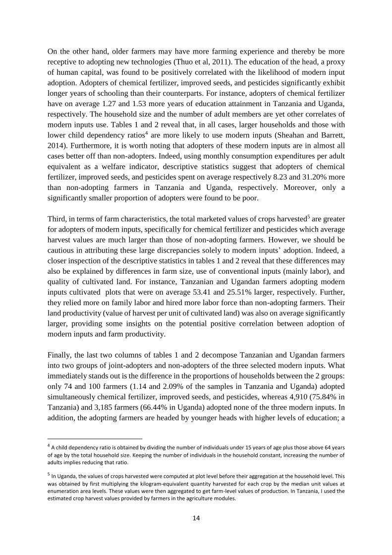
2 depict significant differences between sub-groups of adopters and non-adopters3.

First and unsurprisingly, the rates of modern inputs’ adoption are distressingly low in both

countries. Among all the three selected modern inputs, chemical fertilizer was scarcely applied

(only 7.52 and 4.82% of observations in Tanzania and Uganda, respectively, compared to 11.31

and 13.81% for pesticides or 12.34 and 25.26% for improved seeds), thereby reinforcing the

commonly-held view of low rates of modern input uses in these and other developing countries.

Second, in terms of household characteristics, we note that adopters of either selected modern

input are consistently and significantly younger than non-adopters across both countries.

Theoretically, farmers’ willingness to adopt new technologies might change with age either

positively or negatively. Indeed, as farmers are getting older, they may be more reluctant to

modify their farming habit and take up new agricultural practices or technologies (Simtowe et

al, 2006).

2 1USD 1,654 Tanzanian shillings; 1USD 2,600 Ugandan shillings.

3 It should be borne in mind that these different groups of agricultural households are not mutually exclusive. For instance,

among non-adopters of chemical fertilizer, we also find some adopters of improved seeds and/or pesticides. As shown in the methodological section, this feature justified the use of a multivariate technology adoption model.

14

On the other hand, older farmers may have more farming experience and thereby be more

receptive to adopting new technologies (Thuo et al, 2011). The education of the head, a proxy

of human capital, was found to be positively correlated with the likelihood of modern input

adoption. Adopters of chemical fertilizer, improved seeds, and pesticides significantly exhibit

longer years of schooling than their counterparts. For instance, adopters of chemical fertilizer

have on average 1.27 and 1.53 more years of education attainment in Tanzania and Uganda,

respectively. The household size and the number of adult members are yet other correlates of

modern inputs use. Tables 1 and 2 reveal that, in all cases, larger households and those with

lower child dependency ratios4 are more likely to use modern inputs (Sheahan and Barrett,

2014). Furthermore, it is worth noting that adopters of these modern inputs are in almost all

cases better off than non-adopters. Indeed, using monthly consumption expenditures per adult

equivalent as a welfare indicator, descriptive statistics suggest that adopters of chemical

fertilizer, improved seeds, and pesticides spent on average respectively 8.23 and 31.20% more

than non-adopting farmers in Tanzania and Uganda, respectively. Moreover, only a

significantly smaller proportion of adopters were found to be poor.

Third, in terms of farm characteristics, the total marketed values of crops harvested5 are greater

for adopters of modern inputs, specifically for chemical fertilizer and pesticides which average

harvest values are much larger than those of non-adopting farmers. However, we should be

cautious in attributing these large discrepancies solely to modern inputs’ adoption. Indeed, a

closer inspection of the descriptive statistics in tables 1 and 2 reveal that these differences may

also be explained by differences in farm size, use of conventional inputs (mainly labor), and

quality of cultivated land. For instance, Tanzanian and Ugandan farmers adopting modern

inputs cultivated plots that were on average 53.41 and 25.51% larger, respectively. Further,

they relied more on family labor and hired more labor force than non-adopting farmers. Their

land productivity (value of harvest per unit of cultivated land) was also on average significantly

larger, providing some insights on the potential positive correlation between adoption of

modern inputs and farm productivity.

Finally, the last two columns of tables 1 and 2 decompose Tanzanian and Ugandan farmers

into two groups of joint-adopters and non-adopters of the three selected modern inputs. What

immediately stands out is the difference in the proportions of households between the 2 groups:

only 74 and 100 farmers (1.14 and 2.09% of the samples in Tanzania and Uganda) adopted

simultaneously chemical fertilizer, improved seeds, and pesticides, whereas 4,910 (75.84% in

Tanzania) and 3,185 farmers (66.44% in Uganda) adopted none of the three modern inputs. In

addition, the adopting farmers are headed by younger heads with higher levels of education; a

4 A child dependency ratio is obtained by dividing the number of individuals under 15 years of age plus those above 64 years

of age by the total household size. Keeping the number of individuals in the household constant, increasing the number of adults implies reducing that ratio.

5 In Uganda, the values of crops harvested were computed at plot level before their aggregation at the household level. This

was obtained by first multiplying the kilogram-equivalent quantity harvested for each crop by the median unit values at enumeration area levels. These values were then aggregated to get farm-level values of production. In Tanzania, I used the estimated crop harvest values provided by farmers in the agriculture modules.

15

larger proportion of these joint-adopters are male-headed, with larger household and adult

members.

Table 1. Some descriptive statistics by technology adoption’s status - Tanzania

Variable Description All panel

households

Chemical fertilizer Improved seeds Pesticides Joint

adoption

Non-adoption

Adopters Non-adopters Adopters Non-adopters Adopters Non-adopters

Household characteristics

AGE Age of the head (in years) 47.23

(15.85)

47.13

(15.22)

47.23 (15.89) 46.59

(13.91)

47.32 (16.01) 47.28

(14.75)

47.22 (15.98) 46.42

(15.29)

47.21 (16.24)

EDUC Education of the head (in years) 5.05 (4.05) 6.22 (3.71) 4.95 (4.07)*** 5.74 (3.93) 4.95 (4.06)*** 5.75 (3.69) 4.96 (4.09)*** 6.99 (3.46) 4.86 (4.11)***

GENDER Female-headed household (in %) 0.24 0.18 0.25*** 0.21 0.25** 0.16 0.25*** 0.15 0.26**

HHSIZE Household size (number) 5.32 (2.93) 5.50 (2.43) 5.31 (2.97) 6.18 (3.69) 5.20 (2.79)*** 5.77 (3.65) 5.26 (2.82)*** 5.72 (2.58) 5.16 (2.82)*

NADULT Number of adults 2.80 (1.50) 2.85 (1.28) 2.80 (1.51) 3.15 (1.88) 2.75 (1.43)*** 3.03 (1.79) 2.77 (1.45)*** 3.16 (1.53) 2.76 (1.43)***

ECONS Consumption per adult

equivalent (in USD)

36.139

(29.082)

35.398

(25.306)

36.199

(29.369)

41.654

(30.449)

35.362

(28.803)

39.083

(28.418)

35.763

(29.147)

44.715

(37.485)

35.436

(28.809)

POV Poverty status ( % of poor) 0.07 0.02 0.08*** 0.05 0.08*** 0.03 0.08*** 0.01 0.08**

Farm characteristics

OUTPUT Crop output (in USD) 461.636

(3,679.485)

745.648

(2,043.485)

438.482

(3,780.953)*

703.414

(4,067.932)

427.595

(3,620.545)**

1293.537

(7,315.599)

355.584

(2,890.101)***

839.397

(1,139.268)

457.268

(3,698.472)*

LAND Land size (in acres) 3.89 (10.96) 5.71 (8.78) 3.74 (11.11)*** 5.53 (23.45) 3.66 (7.71)*** 5.71 (8.41) 3.65 (11.22)*** 5.46 (7.98) 3.36 (7.65)**

LPRODV Land productivity (USD/acre) 429.026

(7,738.815)

498.458

(3,082.573)

423.365

(7,980.653)

1,000.729

(16,747.279)

348.534

(5,357.431)**

808.340

(6,408.706)

380.670

(7,859.734)*

727.678

(2,814.137)

291.702

(5,164.640)*

FLABOR Family labor (in person-days) 134.74

(176.57)

186.09

(173.60)

130.55

(176.16)***

143.50

(182.05)

133.51

(175.76)*

213.86

(223.73)

124.65

(166.96)***

188.51

(205.05)

121.73

(167.65)***

HLABOR Hired labor (in person-days) 9.98 (31.82) 19.62

(41.34)

9.19 (30.79)*** 20.24

(54.91)

8.53 (26.72)*** 26.31

(65.72)

7.89 (23.52)*** 33.30

(62.60)

6.84

(11.66)***

EFERT Chemical fertilizer (in USD) 8.087

(69.708)

107.162

(232.254)

- 22.501

(141.693)

6.047

(51.827)***

43.590

(188.412)

3.551 (27.875)*** 189.841

(423.568)

-

ESEEDS Improved seeds (in USD) 3.092

(48.928)

7.206

(34.537)

2.755

(49.9.6)*

25.050

(137.361)

- 13.141

(128.170)

1.811 (24.351)*** 37.635

(81.005)

-

EPEST Pesticides (in USD) 4.688

(69.295)

9.577

(78.480)

4.289

(68.484)*

9.316

(71.928)

4.036

(68.898)**

41.459

(202.489)

- 37.297

(195.507)

-

LDQ Land quality (% with good quality) 0.36 (0.42) 0.43 (0.41) 0.35 (0.43)*** 0.39 (0.42) 0.35 (0.43)** 0.47 (0.16) 0.34 (0.42)*** 0.45 (0.39) 0.34 (0.42)**

LDSP Land slope (% of flatted plots) 0.90 (0.28) 0.97 (0.13) 0.90 (0.28)*** 0.97 (0.14) 0.90 (0.29)*** 0.97 (0.13) 0.89 (0.28)*** 0.98 (0.11) 0.89 (0.30)**

Obs Observations 6,474 488 5,986 799 5,675 732 5,742 74 4,910

Note: ***, **, and * indicate statistically significant differences between the subgroups of adopters and non-adopters of modern inputs using a simple t-test with unequal variances. Standard

deviations into brackets.

17

Table 2. Some descriptive statistics by technology adoption’s status – Uganda

Variable Description All panel

households

Chemical fertilizer Improved seeds Pesticides Joint

adoption

Non-adoption

Adopters Non-adopters Adopters Non-adopters Adopters Non-adopters

Household characteristics

AGE Age of the head (in years) 47.50

(15.01)

46.09

(12.94)

47.57

(15.11)*

46.79

(13.30)

47.72

(15.43)***

46.46

(13.77)

47.66

(15.20)**

46.03

(12.29)

47.78

(15.54)*

EDUC Education of the head (in years) 4.79 (3.79) 6.25 (3.90) 4.72 (3.78)*** 5.46 (3.92) 4.58 (3.73)*** 6.04 (3.79) 4.59 (3.76)*** 6.41 (4.08) 4.45 (3.72)***

GENDER Female-headed household (in

%)

0.29 0.15 0.33*** 0.22 0.31*** 0.18 0.301*** 0.09 0.33***

HHSIZE Household size (number) 7.21 (3.45) 8.30 (3.95) 7.15 (3.41)*** 7.64 (3.47) 7.07 (3.43)*** 8.36 (3.98) 7.02 (3.32)*** 9.17 (4.29) 6.92 (3.33)***

NADULT Number of adults 3.67 (2.29) 4.28 (3.01) 3.64 (2.24)*** 3.91 (2.41) 3.59 (2.24)*** 4.27 (2.77) 3.57 (2.18)*** 4.88 (3.39) 3.52 (2.17)***

ECONS Consumption per adult

equivalent (in USD)

19.85

(48.88)

26.71

(33.59)

19.50

(49.51)***

22.57

(45.49)

18.93

(49.95)

27.63

(80.40)

18.56

(41.23)***

28.16

(36.28)

17.86

(39.26)***

POV Poverty status ( % of poor) 0.33 0.17 0.33*** 0.26 0.34*** 0.19 0.34*** 0.13 0.35***

Farm characteristics

OUTPUT Crop output (in USD) 143.63

(289.06)

333.56

(445.59)

134.01

(275.42)***

193.75

(346.53)

126.69

(264.77)***

302.44

(442.85)

117.15

(244.79)***

437.22

(555.68)

191.40

(332.56)***

LAND Land size (in acres) 3.99 (26.11) 4.14 (8.44) 3.99 (26.69) 5.25 (42.42) 3.60 (17.65)** 4.90

(15.94)

3.86 (27.39) 5.36 (8.84) 3.43 (17.37)*

LPRODV Land productivity (USD/acre) 126.98

(398.92)

214.47

(427.35)

122.55

(396.96)***

153.41

(435.47)

118.05

(385.43)***

193.33

(539.81)

115.92

(369.16)***

201.05

(292.10)

112.19

(364.13)**

FLABOR Family labor (in person-days) 298.78

(296.85)

485.67

(513.43)

289.48

(278.58)***

342.30

(343.80)

284.81

(278.71)***

443.99

(417.26)

275.51

(265.42)***

575.10

(599.52)

268.87

(260.30)***

HLABOR Hired labor (in person-days) 25.80

(74.95)

41.92

(113.75)

25.05

(72.62)*

41.96

(113.16)

21.39 (59.76)* 52.50

(120.31)

22.05

(65.32)***

77.31

(187.89)

19.61

(57.85)***

EFERT Chemical fertilizer (in USD) 1.14

(12.23)

23.59

(50.86)

- 3.52

(23.19)

0.33

(4.00)***

5.38

(22.73)

0.42

(9.23)***

28.69

(49.34)

-

ESEEDS Improved seeds (in USD) 3.12

(16.34)

14.79

(41.57)

2.52

(13.64)***

12.34

(30.72)

- 8.38

(30.07)

2.24

(12.47)***

21.12

(30.57)

-

EPEST Pesticides (in USD) 1.56 (9.67) 10.93

(30.59)

1.08

(6.81)***

3.35 (15.47) 0.95

(6.55)***

10.93

(23.52)

- 19.68

(41.99)

-

LDQ Land quality (% with good

quality)

0.55 (0.43) 0.57 (0.41) 0.55 (0.43) 0.57 (0.42) 0.55 (0.44)* 0.60 (0.41) 0.54 (0.44)*** 0.56 (0.40) 0.54 (0.44)

LDSP Land slope (% of flatted plots) 0.86 (0.30) 0.86 (0.27) 0.86 (0.30) 0.90 (0.24) 0.84 (0.31)*** 0.88 (0.27) 0.85 (0.30)* 0.87 (0.24) 0.84 (0.32)

Obs Observations 4,794 231 4,563 1,211 3,583 685 4,109 100 3,185

Note: ***, **, and * indicate statistically significant differences between the subgroups of adopters and non-adopters of modern inputs using a simple t-test with unequal variances. Standard

deviations into brackets.

Economically, they are better-off than their non-adopter counterparts with larger monthly

consumption per adult equivalent and greater crop production values. On average, they

cultivate significantly larger portions of land and spend more time on farming activities than

non-adopters.

5. RESULTS AND ANALYSIS

This section first presents estimation results of moments of production function a la Antle as

outlined earlier. Then, I present econometric results from the multivariable probit model that

allows for the possibility of simultaneous or multiple technology adoption behavior and

incorporate farmers’ exposure to production risks. Finally, I present the estimated farmers’ risk

premium and certainty equivalent and test for the relationship between the cost of private risk

bearing and technology adoption.

5.1. Moments of the production function

I estimate factors affecting the first four moments (mean, variance, skewness, and kurtosis) of

smallholder farmers’ production levels. The econometric results of the mean equation (14) are

reported in table 3 using the Mundlak-Chamberlain Instrumental variables (IV) fixed effects

model6. In this model specification, both unobserved heterogeneity and endogeneity issues are

treated. Indeed, it is likely that the adoption of modern inputs (chemical fertilizer, improved

seeds, and pesticides) and use of conventional inputs (labor, for example) are endogenous. I

investigated the endogeneity problems using the Durbin-Wu-Hausman test (Davidson and

Mackinnon, 1993; Wooldridge, 2002). Referring to both theory and existing literature

(Koundouri et al, 2005; Di Falco and Chavas, 2009; Juma et al, 2009; Chavas and Di Falco,

2012), I instrumented for endogenous inputs using the age, gender, and education of the

household’s head, distances from homestead to nearest major road, market and population

centers, regional dummies as well as lagged values of endogenous variables.

The relevance of these instruments was assessed by applying an F-test of joint significance of

the excluded instruments. I also performed the Hansen J test to test the overidentification

restrictions. The Durbin-Wu-Hausman F-test was 1.86 (p-value=0.298) and 1.51 (p-value:

0.362) for Tanzania and Uganda, respectively. Contrarily to the standard fixed effects

estimators (see Appendix A.3), Mundlak-Chamberlain IV specifications do not show evidence

of endogeneity bias after controlling for potential correlation between unobserved

heterogeneity h and farmers’ characteristics. Furthermore, the Hansen J test results indicate

that the instruments are uncorrelated with the error term and are thus valid instruments. Table

6 I also used two other alternative specifications (See appendix A.3). A standard fixed-effects model which relies on data

transformation that removes both individual fixed effects and time-invariant covariates and a standard Mundlak-

Chamberlain fixed effects approach which controls for unobserved heterogeneity h but leaves aside the potential

endogeneity of some explanatory variables.

19

3 reports the econometric estimates of the mean equation of the stochastic production function

using a flexible quadratic specification7 in productive inputs:

hthjhtiht

I

i

I

j

ij

I

i

ihtiht XXXy 1

1 11

01 lnln2

1lnln

γΨ'β'Ωht (17)

where hty1 is the total production (in values)8 by farmer h in year t; ihtX is a productive input

i used by farmer h at time t (such as land size, farm labor, improved seeds, chemical fertilizer,

and pesticides); htΩ is a vector of environmental and climatic factors (labor quality, land slope,

average annual temperature in °C, precipitation and rainfall in cm); Ψ denotes a vector of time

dummies; 0 , i , ij , , and are unknown parameter to be estimated; h and ht1 have

been previously defined.

Across the two countries, the econometric estimates appear robust and relatively similar.

Globally, the estimated coefficients are statistically significant and display the expected signs.

Both conventional and modern productive inputs are found statistically significant and

production-increasing. In particular, land characteristics influenced the values of outputs

harvested, which were increasing with land size and proportion of land of good quality. Hence,

a one percent increase of the area cultivated is expected to lead to a 0.37 and 0.53% increase

in the values of crop harvested in Tanzania and Uganda, respectively. In both countries, the use

of modern inputs statistically and positively impact on the output values, suggesting the

potential benefits smallholder Tanzanian and Ugandan farmers could get by increasing their

adoption rates. In addition, output values and expenditures on modern inputs positively

correlate, but only up to a certain level of input costs. However, in both countries, the impact

of chemical fertilizer expenditures is statistically insignificant. This might be imputable to its

limited usage by Tanzanian and Ugandan farmers during the sample period, compared for

instance with the proportions applying improved seeds and pesticide (see tables 1 and 2).

In terms of environmental or climatic variables, results in table 3 reveal an inverted U-shaped

relationship between on the one hand average temperature, precipitation, and rainfall, and on

the other marketed values of crops harvested. Thus, while an increase in the average value of

climatic variables is expected to improve crop production levels, climate effects become

negative after reaching a certain threshold. In Tanzania, these turning points are evaluated at

39.95°C, 167.2 cm and 282.36 cm for average annual temperature, precipitation, and rainfall,

respectively. In Uganda, these threshold values become 33.29°C, 150 cm and 180.37 cm,

respectively. This result underscores the importance of addressing the adverse effects of

climate volatility in developing countries where smallholder farmers are often uninsured

against climatic vagaries (Kassie et al, 2008; Seo and Mendelsohn, 2008; Deressa and Hassan;

7 To include explanatory variables displaying zero values (mainly modern input variables) in the quadratic model

specification, I follow Battese (1997) and Di Falco and Chavas (2009) by applying DXD ln10 , where 1D if

0X , and 0D if X > 0 , with X, the explanatory variables with zero values; and 0 and 1 are unknown parameters

to be estimated.

8 Using values of production instead of physical quantities aims at reflecting the multi-cropping nature of most farmers in

Tanzania and Uganda and enables the aggregation of different crop productions into a single monetary unit.

20

2010: Arslan et al, 2014). Finally, once I control for endogeneity and unobserved heterogeneity,

output values are found less responsive to variations in farm labor than in cultivated land, with

a land production elasticity of 0.73 and 0.53% in Tanzania and Uganda, respectively, against

0.37 and 0.30% for labor elasticity, suggesting that output increases in Tanzania and Uganda’s

agricultural sectors tend to be at the extensive margin (Sherlund et al, 2002).

Table 3. Estimation of the flexible quadratic production function – Mundlak-Chamberlain IV fixed effects model

Variables Tanzania Uganda

Coeffs Std errors Coeffs Std errors

LAND 0.732*** 0.084 0.0534** 0.29

LAND2 0.058 0.097 0.047* 0.014

LABOR 0.37 0.208 0.299** 0.123

LABOR2 -0.033*** 0.008 0.09 0.088

DFERT 0.475*** 0.089 0.211 0.544

EFERT 0.74 0.834 0.358 0.459

EFERT2 -0.069 0.186 -0.296 0.534

DSEEDS 0.116* 0.065 0.988*** 0.06

ESEEDS 0.05 ***0.009 0.978*** 0.299

ESEEDS2 -0.004 0.094 -0.097 0.171

DPEST 0.278* 0.145 0.162** 0.089

EPEST 0.699* 0.353 1.199*** 0.048

EPEST2 -0.026* 0.016 -0.086 0.626

LAND × LABOR 0.037 0.05 0.096* 0.046

LAND×EFERT 0.039 0.055 0.019 0.041

LAND×ESEEDS -0.008 0.026 -0.008 0.051

LAND×EPEST -0.111* 0.062 -0.001 0.028

LABOR ×EFERT 0.048 0.14 -0.013 0.189

LABOR×ESEEDS -0.071*** 0.023 -0.127 0.18

LABOR×EPEST 0.084 0.115 -0.118 0.142

LDQ 0.432* 0.254 0.292* 0.18

LDSP -0.26 0.451 -0.238 0.644

LDSP2 -0.141 0.233 0.184 0.331

LTEMP 51.372* 30.007 23.041** 9.751

LTEMP2 -0.643*** 0.028 -0.346* 0.184

LPREC 5.016 12.816 25.801*** 8.713

LPREC2 -0.015 1.579 -0.086*** 0.019

LRAIN 11.859** 4.69 26.334*** 8.293

LRAIN2 0.021 0.063 -0.073*** 0.019

YR(a) 0.326 0.233 0.421** 0.18

Cons -75.651 63.867 -14.096*** 2.665

Observations 4,316 3,196

Note: (a): YR stands for a dummy variable taking 1 if it is the last survey (2012/13 in Tanzania and 2011/12 in Uganda) and 0

otherwise. Predicted mean production values: 483.87 USD in Tanzania and 165.29 USD in Uganda. Hansen J-test statistic

for Tanzania: 3.630; 62 ; p-value: 0.511; and for Uganda: respectively: 3.515; 62 ; p-value: 0.742. Durbin-Wu-

Hausman endogeneity test for Tanzania: F-test= 1.86 (p-value=0.298); and for Uganda: F-test= 1.51 (p-value=0.362). ***, **,

and * denote significance levels at 1%, 5%, and 10%, respectively. Whilte’s robust standard errors were used.

The regression results for higher-order moments (variance, skewness, and kurtosis) are

reported in tables 4 and 5 respectively for Tanzania and Uganda using equation (15) and

applying the Mundlak-Chamberlain IV Fixed effects model. The same set of explanatory

variables used in the estimation of the mean equation is also included here. First, in terms of

variance of the production function, most inputs are still statistically significant. However, the

nature of their impact on the production variance appears to be input-specific. Indeed, the

results reveal that, while the use of modern inputs are risk-reducing in both countries (negative

21

coefficients of DFERT, DSEED, and DPEST), their costs are instead risk-increasing, results in

line with other empirical findings by Just and Pope (1979), Rosegrant and Roumasset (1985),

Abedullah and Pandey (2004), and Di Falco and Chavas (2012), among others. Other variables,

such as land size, farm labor, and the proportion of plots of good quality are risk-decreasing.

Intuitively, the risk-reducing effect of farm labor may be explained by the fact that more labor

can help farmers monitor more meticulously crop planting and harvesting processes and

subsequently reduce production variability (Groom et al, 2008). The estimates in tables 4 and

5 also show that all climatic variables increase production variance, highlighting the negative

impact of exposure to climate shocks on production uncertainty. However, since the variance

estimation equation fails to distinguish between upside and downside risks, it is also worth

investigating the effects of different covariates on the skewness function. These effects are

displayed in the third columns of tables 4 and 5.

Table 4. Estimation results of the variance, skewness, and kurtosis functions – Tanzania

Variables Variance function Skewness function Kurtosis function

Coeffs Std errors Coeffs Std errors Coeffs Std errors

LAND -3.940*** 0.979 -0.446*** 0.195 -0.139*** 0.002

LAND2 -0.684 0.882 0.822** 0.403 0.179** 0.083

LABOR -29.851 29.084 -212.004 2,818.257 2.435*** 0.421

LABOR2 6.93 6.103 97.078 591.353 -0.455*** 0.090

DFERT -17.794*** 1.803 3.031*** 0.175 -96.803** 39.799

EFERT 2.757*** 0.466 -514.083*** 45.194 21.315* 10.899

EFERT2 354.083*** 84.451 43.940*** 4.948 2.024* 1.203

DSEEDS 9.185 8.164 2.985*** 0.791 -255.164*** 87.339

ESEEDS -1.884 1.675 -0.616*** 0.162 50.621*** 8.279

ESEEDS2 316.324 280.328 103.698*** 27.165 5.035 3.851

DPEST -7.965* 3.890 582.121 817.213 -9.621*** 0.823

EPEST 1.766* 0.987 -117.132 177.540 1.587*** 0.422

EPEST2 -303.901* 187.174 11.52 18.137 -0.176 2.567

LAND×LABOR -4.147 3.547 77.426 343.276 0.099** 0.040

LAND×EFERT 6.277* 3.504 332.056 378.278 0.000 0.046

LAND×ESEEDS 2.159 1.821 144.571 176.462 0.022 0.019

LAND×EPEST 9.392*** 4.448 -265.515 431.040 -0.047 0.055

LABOR ×EFERT -8.137 9.970 -0.853 0.584 0.302** 0.149

LABOR×ESEEDS -0.568 1.633 304.873* 158.287 -0.015 0.017

LABOR×EPEST -12.808 7.156 125.902 790.303 0.066 0.121

LDQ 7.096 18.807 2.259* 1.102 0.175 0.209

LDSP 20.419 32.113 1.838 1.881 -0.731* 0.377

LDSP2 -8.185 16.615 86.786 415.891 0.116 0.214

LTEMP -1,308.53 2,421.256 11.677*** 4.185 -167.589*** 28.934

LTEMP2 207.539*** 29.189 -5.052 25.145 26.827*** 5.115

LPREC 267.765*** 12.459 50.060*** 5.458 -18.332* 10.919

LPREC2 -17.461 12.442 -5.052 25.145 2.248* 1.339

LRAIN 313.222*** 44.389 -55.833*** 9.470 -20.962** 10.052

LRAIN2 -56.184*** 16.501 -7.59 6.825 2.173 1.379

YR2011 15.83 16.589 -205.356 1,607.509 0.242 0.171

Cons 883.664 4,547.211 -46.407 266.404 346.571*** 55.334

Note: ***, **, and * denote significance levels at 1%, 5%, and 10%, respectively. Whilte’s robust standard errors were used.

Table 5. Estimation results of the variance, skewness, and kurtosis functions – Uganda

Variables Variance function Skewness function Kurtosis function

Coeffs Std errors Coeffs Std errors Coeffs Std errors

22

LAND -540.890** 246.342 117.878*** 41.233 -47.639** 22.013

LAND2 7.684 38.921 -5.431* 2.878 2.853* 1.531

LABOR -1,308.735* 689.258 -54.965 59.911 46.751 31.885

LABOR2 0.048* 0.029 9.287 7.342 -5.811 3.920

DFERT -47.432* 27.239 0.089*** 0.008 -15.260* 6.550

EFERT 9.923* 6.149 0.190* 0.096 32.006*** 12.550

EFERT2 -1311.160 1804.970 -24.368 21.703 -1.805 1.003

DSEEDS -691.771*** 259.751 85.803*** 26.558 -27.124* 14.374

ESEEDS 1,101.909*** 264.342 33.421* 15.214 6.639** 3.612

ESEEDS2 -54.849 152.985 -2.408 14.601 -0.296 7.842

DPEST -43.041*** 18.793 0.302*** 0.045 -613.314*** 62.889

EPEST 9.458* 5.779 0.067* 0.024 136.085*** 13.046

EPEST2 -4.964 0.343 -0.004** 0.002 70.883 72.563

LAND×LABOR 87.882*** 22.898 -17.351*** 7.219 -7.207* 3.853

LAND×EFERT -25.996* 12.249 2.479 3.416 -1.177 1.820

LAND×ESEEDS -15.265 52.517 2.520 4.374 -1.798 2.349

LAND×EPEST -15.589 40.676 -2.114 2.354 1.438 1.255

LABOR ×EFERT 13.933* 6.391 -15.437 15.964 10.308 8.518

LABOR×ESEEDS 71.327 158.994 -1.111 15.485 -0.519 8.316

LABOR×EPEST 43.630 70.748 6.424 12.202 -6.127 6.526

LDQ -330.321* 153.481 36.233** 15.115 14.552* 8.038

LDSP 3.729* 2.228 0.000 0.021 -1.289 28.900

LDSP2 -0.974 0.631 0.005 0.011 -6.200 14.821

LTEMP 1.909*** 0.323 0.088** 0.034 -105.360** 48.454

LTEMP2 -81.590*** 14.851 -3.582** 1.834 2.615* 1.642

LPREC 1.772*** 0.246 0.083*** 0.028 -98.069** 40.886

LPREC2 -478.268*** 66.380 -0.696*** 0.086 1.354** .340

LRAIN -1.165*** 0.154 0.074*** 0.028 -68.925* 37.02

LRAIN2 320.400*** 46.566 -0.576** 0.262 0.029* 0.011

YR2011 -40.852 150.642 -21.991 14.807 17.492** 7.859

Cons 527.286*** 178.759 -112.199 78.516 104.569 36.575

Note: ***, **, and * denote significance levels at 1%, 5%, and 10%, respectively. Whilte’s robust standard errors were used.

All modern inputs are positively and strongly correlated with the skewness of the crop outputs.

This implies that both the use of and the expenditures on these inputs hedged against the risk

of crop failure. The application of chemical fertilizer, improved seeds, and pesticides in the

Tanzanian and Ugandan agricultural sectors is therefore associated with the reduction in

farmers’ exposure to downside risk and acts as an insurance against production fall. In regards

to conventional inputs, only land size and cultivated soil of good quality significantly decrease

the exposure to downside risk. Labor use and land slope are not statistically significantly. The

estimates also indicate that the production skewness has an inverted U-shaped curve in relation

with climatic variables. These variables are expected to protect farmers from downside risk but

only up to a certain threshold beyond which exposure to climate disruptions has detrimental

production effects.

Finally, the reported coefficients for the kurtosis estimation give the impact of covariates on

the peakedness and tailedness of the production distribution. The econometric estimates

suggest that the use of modern inputs statistically influence the kurtosis of crop production

values. More specifically, the estimates indicate that the adoption of chemical fertilizer,

improved seeds, and pesticides are kurtosis decreasing, contrarily to expenditures on these

inputs. Farm size and climatic variables also significantly reduce the degree of production

kurtosis in both countries though at different rates.

23

5.2. Multiple adoption estimation results

The econometric results of the multivariate adoption model using the multivariate probit model

are reported in tables 6 and 7. The model analyzes factors that simultaneously affect the

probability of adopting each of the three modern inputs. The model was estimated using the

Simulated Maximum Likelihood and the GHK simulator, with unobserved heterogeneity

controlled for a la Mundlak-Chamberlain (Mundlak, 1978; Chamberlain, 1980). As suggested

by Cappellari and Jenkins (2003), I chose the number of draws (150)9 greater than the squared

root of the sample sizes to reduce the simulation bias. I also derived starting values from

univariate probit regressions (Cappellari and Jenkins, 2006; Fezzi and Bateman, 2011).

First, all the coefficients of pairwise correlations between error terms ( ij ) are statistically

significant, suggesting a statistical and significant interdependence of adoption decisions. This

result is also confirmed by the significance of the LR test which rejects the null hypothesis that

ij are jointly insignificant. A single equation approach would therefore be restrictive and yield

unreliable results insofar as the likelihood of applying one modern input is conditional on the

adoption or not of other inputs (Zepeda, 1994; Dorfman, 1996).

The econometric estimates shown in tables 6 and 7 highlight the central role played by expected

outputs and production risk variables (variance, skewness, and kurtosis) in shaping farmers’

decisions to using modern inputs. The results indicate that the first moment of production is

positive and strongly significant across all the individual adoption models and across countries:

the higher the expected production levels, the greater the likelihood of technology adoption.

This implies that Tanzanian and Ugandan farmers tend to develop a profit/production-

maximizing behavior when deciding whether to adopt or not modern inputs. As smallholder

and subsistence farmers, they would be persuaded to apply modern inputs and bear their

purchasing costs if their usage could make any significant and positive dent in the increase of

the expected end-of-season output values.

Additionally, production volatility, captured here by the estimated second moment, is found to

negatively impact the probability of applying each selected modern input. This finding

indicates that these smallholder farmers are risk averse inasmuch as the propensity to use

modern inputs is decreasing as the uncertainty about production levels increases. These farmers

would therefore choose less risky activities at the expense of higher investment returns. Similar

results were found by Koundouri et al (2006), Simtowe et al (2006), and Ogada et al (2014).

The statistical significance of the predicted skewness implies that Tanzanian and Ugandan

farmers are also examining the possibility of crop failure when making input adoption

decisions.

9 A sensitive analysis was performed using different number of draws (200, 300, and 500). Although the parameter estimated

quantitatively changed across the number of draws, they remained qualitatively similar.

24

Table 6. Estimation results for the probability of multiple technology adoption – Trivariate probit model - Tanzania

Variables Chemical fertilizer Improved seeds Pesticides

Coeffs Std errors Coeffs Std errors Coeffs Std errors

Production risks

PMEAN 0.053*** 0.012 0.037** 0.013 0.082* 0.035

PVARIANCE -0.009*** 0.001 -0.003*** 0.000 -0.026*** 0.006

PSKEWNESS 0.002*** 0.000 0.001*** 0.000 0.004** 0.002

PKURTOSIS -0.000*** 0.000 -0.000*** 0.000 -0.001*** 0.000

Household characteristics

AGE 0.053*** 0.012 0.037** 0.013 0.082* 0.035

AGE2 -0.009*** 0.001 -0.003*** 0.000 -0.026*** 0.006

HHSIZE 0.002 0.002 0.001 0.000 0.004 0.003

NADULT -0.000*** 0.000 -0.000*** 0.000 -0.001*** 0.000

EDUC 0.053*** 0.012 0.037** 0.013 0.082* 0.035

GENDER -0.009*** 0.001 -0.003*** 0.000 -0.026*** 0.006

Land characteristics

LAND 0.154*** 0.039 0.058* 0.031 0.185*** 0.030

LDQ 0.199** 0.082 0.142* 0.075 0.323*** 0.072

LDSP 0.150*** 0.051 0.527*** 0.118 0.717*** 0.115

LDIR 1.344*** 0.246 0.603*** 0.217 1.471*** 0.206

Climatic characteristics

LTEMP -3.569*** 0.285 -1.578*** 0.262 -1.754*** 0.283

LPREC 0.236 0.153 -0.804*** 0.12 -0.145 0.115

LRAIN 0.614*** 0.147 0.092 0.022*** 0.639*** 0.094

Distance variables

DROAD -0.004*** 0.002 -0.003*** 0.001 -0.001 0.001

DCENTER -0.003** 0.001 -0.001* 0.001 -0.002*** 0.001

DMARKET -0.001* 0.001 0.000 0.000 -0.001** 0.000

Regional and time fixed effects

Dar-es-salam -0.459-** 0.252 0.117 0.183 -0.169 0.243

Arusha -1.450*** 0.492 -0.055 0.15 -0.176 0.219

YR2011 -0.139 0.089 -0.641*** 0.078 0.042 0.072

YR2013 -0.094 0.111 0.554*** 0.076 0.216*** 0.08

Cons 4.026*** 1.091 6.249*** 1.028 0.664 1.147

ij

j1 1 -0.042 0.051 0.112** 0.051

j2

1 0.337*** 0.041

j3

1

1Pr ky

0.838 0.65 0.521

Note: Bootstrapped standard errors are reported. ***, **, and * indicate statistical significance at the 1, 5, and 10% levels,

respectively. ij stands for the coefficient of the correlation between error terms of modern inputs i and j. Likelihood of all

000.04.858,7:,0 23 valuepjiij

Table 7. Estimation results for the probability of multiple technology adoption – Trivariate probit model - Uganda

Variables Chemical fertilizer Improved seeds Pesticides

25

Coeffs Std errors Coeffs Std errors Coeffs Std errors

Production risks

PMEAN 0.278*** 0.013 0.221*** 0.067 0.706*** 0.091

PVARIANCE -0.053* 0.028 -0.042* 0.004 -0.015*** 0.001

PSKEWNESS 0.008*** 0.001 0.013*** 0.009 0.001*** 0.000

PKURTOSIS -0.035 0.053 -0.006* 0.003 -0.001* 0.000

Household characteristics

AGE 0.092*** 0.021 0.105*** 0.016 -0.004 0.017

AGE2 -0.001*** 0.000 -0.001*** 0.000 0.000 0.000

HHSIZE -0.004 0.020 -0.088*** 0.239 -0.053*** 0.021

NADULT -0.027 0.032 -0.075** 0.0329 -0.047 0.031

EDUC 0.028 0.020 0.003 0.017 0.011* 0.006

GENDER -0.409*** 0.125 -0.305*** 0.085 -0.230** 0.102

Land characteristics

LAND 0.089*** 0.053 0.012*** 0.004 0.122*** 0.042

LDQ 0.056 0.103 0.004 0.078 0.197* 0.104

LDSP 0.392*** 0.154 0.430*** 0.197 -0.602** 0.236

LDIR 0.305 0.277 -0.188 0.158 -0.391 0.249

Climatic characteristics

LTEMP -0.770 0.782 -0.411*** 0.058 -0.594*** 0.374

LPREC 0.181*** 0.012 -0.713 0.829 0.468*** 0.063

LRAIN 0.845* 0.439 0.414*** 0.077 0.233*** 0.064

Distance variables

DROAD -0.029*** 0.008 -0.008 0.006 -0.015** 0.006

DCENTER -0.006* -0.003 -0.007*** 0.002 -0.011*** 0.004

DMARKET -0.003 0.003 -0.001 0.002 -0.005 0.003

Regional and time fixed effects

CENTR 0.428*** 0.024 0.632*** 0.151 0.403*** 0.193

EAST 0.033*** 0.002 0.957*** 0.152 0.894*** 0.191

NORTH 0.419*** 0.197 0.274*** 0.014 0.647*** 0.191

YR2010 -0.471** 0.186 -0.507*** 0.134 -0.153 0.122

YR2011 -0.099 0.169 -0.144 0.129 -0.739 0.137

Cons -0.932* 0.552 0.744 0.923 -0.249 0.998

ij

j1 1 0.433*** 0.088 0.308*** 0.083

j2

1 0.058*** 0.007

j3

1

1Pr ky

0.521 0.530 0.618

Note: Bootstrapped standard errors are reported. ***, **, and * indicate statistical significance at the 1, 5, and 10% levels,

respectively. ij stands for the coefficient of the correlation between error terms of modern inputs i and j. Likelihood of all

000.0,02.144,1:,0 23 valuepjiij

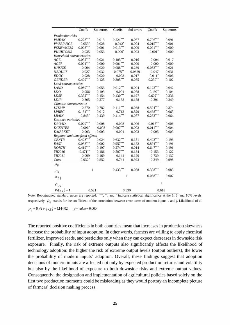
The reported positive coefficients in both countries mean that increases in production skewness

increase the probability of input adoption. In other words, farmers are willing to apply chemical

fertilizer, improved seeds, and pesticides only when they can expect decreases in downside risk

exposure. Finally, the risk of extreme outputs also significantly affects the likelihood of

technology adoption: the higher the risk of extreme output levels (output outliers), the lower

the probability of modern inputs’ adoption. Overall, these findings suggest that adoption

decisions of modern inputs are affected not only by expected production returns and volatility

but also by the likelihood of exposure to both downside risks and extreme output values.

Consequently, the designation and implementation of agricultural policies based solely on the

first two production moments could be misleading as they would portray an incomplete picture

of farmers’ decision making process.

26

Besides production risk variables, other covariates are also of particular interest in explaining

adoption decisions of Tanzanian and Ugandan farmers. However, in contrast to production risk

measures, the effects of household characteristics are heterogeneous and depend on the type of

modern inputs and variables considered. Hence, household size and the number of adults

negatively influenced the probability of using each selected modern input. However, the effect

of household size is not statistically significant for all modern inputs in Tanzania while in

Uganda, only improved seeds and pesticides are significantly affected. These negative

coefficients may be rather explained by the capital intensive nature of modern inputs. Indeed,

as labor-saving techniques, these inputs are more attractive for small-sized households or

farmers with little number of adult members (Asfaw et al, 2014). On the other hand, increases

in the household size and number of adults may encourage farmers to rely mainly on available

family force, which is generally cheaper and sometimes freely accessible. Years of education

attained by the household’s head are associated with increases in the probability of technology

adoption.

This finding is consistent with many other existing studies which have pointed out the positive

and significant correlation between the level of education and technology adoption (Koundouri

et al, 2006; Juma et al, 2009; Kassie et al, 2011; Teklewold, 2013). The econometric results

also indicate life-cycle effects in the adoption of modern inputs: in Uganda, for instance, the

propensity of adoption tends to increase with the age of the head but up to a certain point – at

46 and 52.5 years of age in the case of chemical fertilizer and improved seeds - before

eventually starting to decline. Tables 6 and 7 also highlight the existence of gender disparity in

modern inputs’ adoption. Female-headed households are less likely to use chemical fertilizer,

improved seeds, and pesticides. However, in Tanzania, the gender coefficient is only

statistically significant in the pesticides’ equation. Similar to other developing countries,

Tanzanian and Ugandan female farmers are handicapped by lower access to sufficient

resources and information on modern inputs than their male counterparts.

Farm characteristics also play a significant role in affecting technology’s adoption behavior. In

all cases, the propensity to adopt modern inputs is increasing with land size: the larger the

surface of plots to be cultivated, the more likely the utilization of modern inputs by farmers. In

this context, the adoption of modern inputs may be an efficient means of achieving higher

productivity while reducing the need for labor force. The use of modern inputs is also higher

on flatted and gentile slopes. Contrary to Tanzania, application of modern inputs by Ugandan

farmers was insensitive to whether agricultural plots are irrigated or not.

The analysis also reveals that the usage of the three selected inputs is positively correlated with

soil quality, result in line with findings by Freeman and Omiti (2003) who showed that in semi-

arid areas of Kenya, regions with better soil quality are likely to adopt chemical fertilizer.

Consistent with previous studies (Pender and Gebremedhin, 2007; Teklewold et al, 2013;

Asfaw et al, 2014), inputs’ adoption is further linked to climatic variables. The estimates first

underscore the importance of rainfall availability in explaining adoption behavior of Tanzanian

and Ugandan farmers. I found that the application of modern inputs is of a positive occurrence

in regions where average annual rainfall levels are higher. Similarly, annual precipitation levels

27

also positively affected the propensity of utilization of modern inputs, especially for improved

seeds in Tanzania; and chemical fertilizer and pesticides in Uganda. On the other hand, results

revealed that in regions with higher temperatures, the likelihood of modern inputs adoption

was lower, though insignificant for chemical fertilizer in Uganda. These results are consistent

with findings by Kassie et al (2010), Thuo et al (2011), Teklewold et al (2013), and Asfaw et

al (2014) who obtained a significant relationship between yield enhancing inputs and climatic

variability.

Distance variables also influence farmers’ attitude towards adoption of modern inputs.

Estimates indicate that the greater the distance of the dwelling to either the nearest major road,

population center, or market, the higher the disincentive to use modern inputs. Indeed, longer

distances are associated with higher transportation costs, especially in developing countries

such as Tanzania and Uganda where rural transport infrastructures are poorly developed.

However, similarly to other discrete choice models, the parameter estimates reported in tables

6 and 7 are not per se informative of the marginal effects of the covariates on the adoption

probabilities. To analyze these marginal effects and therefore be able to identify which

independent variables explain the most the observed changes in the probability of modern input

uses, I display in tables 8 and 9 the marginal effects defined as the impact of changes in the

exogenous variables on the changes in the probability of adoption. To evaluate the marginal

effect of a covariate jz on each of the three modern inputs, I followed Greene (2002, p. 668)

and calculated a linear prediction on each technology adoption and, using

ijiji ZzZyE ˆˆ'/ , I averaged out the marginal effects for each observation, where ij

is the estimated coefficient of jz in the ith adoption model , and i = chemical fertilizer,

improved seeds, and pesticides; . is the density function of the standard normal distribution

with mean 0 and variance 1.

The reported marginal effects suggest that the expected mean and variance of production levels

are among the most important factors driving changes in the probabilities of adoption.

However, these marginal effects are heterogeneous across technology adoption equations and

countries. More specifically, a 1% increase in the expected production levels in Uganda is

likely to increase the probability of adopting chemical fertilizer by 0.05% against 0.10% for

improved seeds and 0.09% for pesticides. These marginal effects drop respectively to 0.03,

0.03, and 0.01% in Tanzania. Furthermore, though smaller compared to the impact of changes

in expected production returns, a 10% change in the volatility of production levels is expected

to discourage modern inputs’ application by 0.04 (0.17), 0.06 (0.09), and 0.03% (0.82%) in

Tanzania (Uganda) for chemical fertilizer, improved seeds, and pesticides, respectively. The

marginal effects of production risk variables are then decreasing, in absolute values, as we go

further with higher-order central moments. Table 8. Marginal effects of explanatory variables – Trivariate probit model – Tanzania

Variables Chemical fertilizer Improved seeds Pesticides

Coeffs Std errors Coeffs Std errors Coeffs Std errors

Production risks

PMEAN 0.032 0.019 0.034 0.042 0.014** 0.006

28

PVARIANCE -0.004*** 0.001 -0.006*** 0.000 -0.003*** 0.000

PSKEWNESS 0.001*** 0.000 0.002*** 0.000 0.001** 0.000

PKURTOSIS -0.001 0.001 -0.002*** 0.001 -0.000*** 0.000

Household characteristics

AGE 0.032 0.019 0.034 0.042 0.014** 0.006

AGE2 0.004*** 0.001 0.006*** 0.000 0.003*** 0.000

HHSIZE -0.001*** 0.000 -0.002*** 0.000 -0.001** 0.000

NADULT -0.001 0.001 -0.002*** 0.001 -0.000*** 0.000

EDUC 0.032 0.019 0.034 0.042 0.014** 0.006

GENDER -0.004*** 0.001 -0.006*** 0.000 -0.003*** 0.000

Land characteristics

LAND 0.009*** 0.002 0.006* 0.003 0.017*** 0.004

LDQ 0.005 0.003 0.012 0.008 0.034*** 0.007

LDSP 0.015** 0.008 0.047** 0.019 0.058*** 0.014

LDIR 0.052*** 0.011 0.091*** 0.025 0.163*** 0.024

Climatic variables

LTEMP -0.188*** 0.026 -0.185*** 0.038 -0.298*** 0.04

LPREC 0.011 0.008 -0.065*** 0.017 -0.031** 0.015

LRAIN 0.017** 0.007 0.047*** 0.015 0.031** 0.013

Distance variables

DROAD -0.000** 0.000 -0.000*** 0.000 -0.000 0.000

DCENTER -0.000 0.000 -0.000** 0.000 0.000*** 0.000

DMARKET 0.000 0.000 0.000 0.000 0.000 0.000

Regional and time fixed effects

Dar-es-Salam -0.009 0.016 -0.032 0.023 -0.083** 0.037

Arusha -0.040*** 0.014 -0.007 0.02 -0.018 0.022

YR2011 -0.013*** 0.003 -0.103*** 0.011 -0.002 0.006

YR2013 -0.012*** 0.004 0.070*** 0.009 0.012 0.008

Note: Bootstrapped standard errors are reported. ***, **, and * indicate statistical significance at the 1, 5, and 10% levels,

respectively.

In terms of household characteristics, the estimated marginal effects, evaluated at the sample

means, show that a 10% increase in the number of household members would significantly

decrease the propensity of adoption in Tanzania by 0.02% for improved seeds, while in

Uganda, the likelihood of applying chemical fertilizer and pesticides would decline by 0.01%

and by 0.05% for improved seeds. Among the selected household characteristics, gender of the

household head explained the most the dis-adoption propensity of chemical fertilizer (-0.004%)

and pesticides (-0.003%) among small-scale Tanzanian farmers. In Uganda, years of education

of the head were instead the most contributing factor (0.08%) to the application of chemical

fertilizer, while gender of the head reduced the most the likelihood of using improved seeds (-

0.064%) and pesticides (-0.013%).

With regards to land characteristics, a percent increase in land size increase the probability of

using chemical fertilizer, improved seeds, and pesticides by respectively 0.009, 0.006 and

0.017% in Tanzania and by 0.10, 0.004, and 0.011% in Uganda. These results, in line with

other previous empirical studies (Isham, 2002; Thuo et al, 2011; Dercon and Christiaensen,

2011), also suggest that demand and access to modern agricultural inputs would be easier as

farms get larger inasmuch as their holders can afford the high costs of input purchases or

provide credible collateral to financial institutions. Dercon and Christiaensen (2011) found for

example that the majority of Ethiopian farmers mentioned high purchasing costs as the most

important raisons for not applying modern inputs. As per climatic factors, changes in average

rainfall, precipitation, and temperature had, in absolute values, the highest impacts on

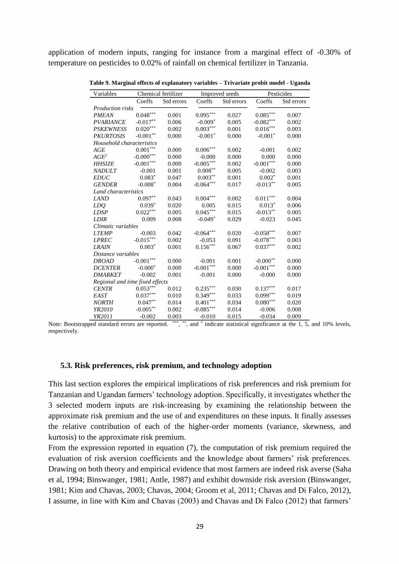
29

application of modern inputs, ranging for instance from a marginal effect of -0.30% of

temperature on pesticides to 0.02% of rainfall on chemical fertilizer in Tanzania.

Table 9. Marginal effects of explanatory variables – Trivariate probit model - Uganda

Variables Chemical fertilizer Improved seeds Pesticides

Coeffs Std errors Coeffs Std errors Coeffs Std errors

Production risks

PMEAN 0.048*** 0.001 0.095*** 0.027 0.085*** 0.007

PVARIANCE -0.017** 0.006 -0.009* 0.005 -0.082*** 0.002

PSKEWNESS 0.020*** 0.002 0.003*** 0.001 0.016*** 0.003

PKURTOSIS -0.001** 0.000 -0.001* 0.000 -0.001* 0.000

Household characteristics

AGE 0.001*** 0.000 0.006*** 0.002 -0.001 0.002

AGE2 -0.000*** 0.000 -0.000 0.000 0.000 0.000

HHSIZE -0.001*** 0.000 -0.005*** 0.002 -0.001*** 0.000

NADULT -0.001 0.001 0.008** 0.005 -0.002 0.003

EDUC 0.083* 0.047 0.003** 0.001 0.002* 0.001

GENDER -0.008* 0.004 -0.064*** 0.017 -0.013** 0.005

Land characteristics

LAND 0.097** 0.043 0.004*** 0.002 0.011*** 0.004

LDQ 0.039* 0.020 0.005 0.015 0.013* 0.006

LDSP 0.022*** 0.005 0.045*** 0.015 -0.013** 0.005

LDIR 0.009 0.008 -0.049* 0.029 -0.023 0.045

Climatic variables

LTEMP -0.003 0.042 -0.064*** 0.020 -0.058*** 0.007

LPREC -0.015*** 0.002 -0.053 0.091 -0.078*** 0.003

LRAIN 0.003* 0.001 0.156*** 0.067 0.037*** 0.002

Distance variables

DROAD -0.001*** 0.000 -0.001 0.001 -0.000** 0.000

DCENTER -0.000* 0.000 -0.001*** 0.000 -0.001*** 0.000

DMARKET -0.002 0.001 -0.001 0.000 -0.000 0.000

Regional and time fixed effects

CENTR 0.053*** 0.012 0.235*** 0.030 0.137*** 0.017

EAST 0.037*** 0.010 0.349*** 0.033 0.099*** 0.019

NORTH 0.047** 0.014 0.401*** 0.034 0.080*** 0.020

YR2010 -0.005** 0.002 -0.085*** 0.014 -0.006 0.008

YR2011 -0.002 0.003 -0.010 0.015 -0.034 0.009

Note: Bootstrapped standard errors are reported. ***, **, and * indicate statistical significance at the 1, 5, and 10% levels,

respectively.

5.3. Risk preferences, risk premium, and technology adoption

This last section explores the empirical implications of risk preferences and risk premium for

Tanzanian and Ugandan farmers’ technology adoption. Specifically, it investigates whether the

3 selected modern inputs are risk-increasing by examining the relationship between the

approximate risk premium and the use of and expenditures on these inputs. It finally assesses

the relative contribution of each of the higher-order moments (variance, skewness, and

kurtosis) to the approximate risk premium.

From the expression reported in equation (7), the computation of risk premium required the

evaluation of risk aversion coefficients and the knowledge about farmers’ risk preferences.

Drawing on both theory and empirical evidence that most farmers are indeed risk averse (Saha

et al, 1994; Binswanger, 1981; Antle, 1987) and exhibit downside risk aversion (Binswanger,

1981; Kim and Chavas, 2003; Chavas, 2004; Groom et al, 2011; Chavas and Di Falco, 2012),

I assume, in line with Kim and Chavas (2003) and Chavas and Di Falco (2012) that farmers’

30

risk preferences can be defined by a utility function exhibiting a constant relative risk aversion

(CRRA) of the form of 1/1U , where is the Arrow-Pratt coefficient of relative

risk aversion. Using equation (7), this means that:

/

22

2

U

Ur ; 2

33

3 /1

U

Ur , and 3

44

4 /21

U

Ur (18)

In this case, the approximate risk premium can be written as:

432 ˆ2124

1ˆ1

6

1ˆ

2

1~ R (19)

where j , with j =2, 3, 4 are the estimated central moments.

The empirical evidence has shown that while it is reasonable that risk preferences substantially

differ across individuals, the coefficient of relative risk aversion is typically found within

the range 1 to 4 (Gollier, 2001). Table 10 reports summary statistics of the approximate risk

premium R~

derived from equation (19) using alternative values of the coefficient ( = 1;

1.5; 2; 2.5; 3; 3.5; and 4). As expected, the risk premium are increasing with the Arrow-Pratt

coefficient of relative risk aversion, ranging from 19.61 USD (15.31 USD) when 1 to

224.05 USD (85.07 USD) when 4 in Tanzania (Uganda). In addition, expressed in terms

of expected production revenues, estimates show that moderate risk-averse Tanzanian and

Ugandan farmers (with 2 ) are willing to give up respectively 12.7% and 30.5% of their

expected revenues to get a certain production revenue in the future. Similar results have been

reported by Groom et al (2008) who found that risk-averse Cypriot farmers had an estimated

risk premium of 17.1 and 22.2% for cereals and vegetables, respectively. Using equation (19),

it is also possible to determine which proportion of the estimated risk premium is attributed to

the different central moments of production. Results reported in table 10 indicate that the

largest part of the estimated risk premium is attributed to production variance (69.3% in

Tanzania and 60.9% in Uganda), followed by production skewness (27% in Tanzania and

36.9% Uganda) while the contribution of kurtosis is very marginal (3.2 and 2.2% in Tanzania

and Uganda, respectively). Finally, in terms of certainty equivalent ( EC~

), table 10 shows that,

as expected, its values are decreasing as farmers become more risk averse.

Given the approximate risk premium, it is possible to examine the relationship between the

cost of private risk bearing and technology adoption. To that end, I regressed the risk premium

(with = 2) on modern inputs’ use and purchasing costs using an Instrumental Variables – 2

Stage Least Square (IV-2SLS) estimation method to deal with the endogeneity of these

covariates. The econometric estimates, reported in appendix A.4, are in accordance with the

previous findings that, while the use of chemical fertilizer, improved seeds, and pesticides is

risk-decreasing, their purchasing costs are instead risk-increasing: the more Tanzanian and

Ugandan farmers have to spend on modern inputs, the higher the cost of private risk bearing

(i.e. the higher the risk premium). For instance, appendix A.4 indicates that a one percent

increase in the purchasing costs of chemical fertilizer is likely to raise farmers’ risk premium

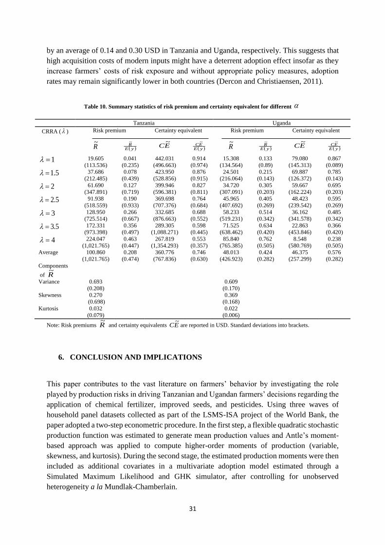
31

by an average of 0.14 and 0.30 USD in Tanzania and Uganda, respectively. This suggests that

high acquisition costs of modern inputs might have a deterrent adoption effect insofar as they

increase farmers’ costs of risk exposure and without appropriate policy measures, adoption

rates may remain significantly lower in both countries (Dercon and Christiaensen, 2011).

Table 10. Summary statistics of risk premium and certainty equivalent for different

Tanzania Uganda

CRRA ( ) Risk premium Certainty equivalent

Risk premium Certainty equivalent

R~

yER~

EC~

yEEC~

R~

yER~

EC~

yEEC~

1 19.605

(113.536)

0.041

(0.235)

442.031

(496.663)

0.914

(0.974)

15.308

(134.564)

0.133

(0.89)

79.080

(145.313)

0.867

(0.089)

5.1 37.686

(212.485)

0.078

(0.439)

423.950

(528.856)

0.876

(0.915)

24.501

(216.064)

0.215

(0.143)

69.887

(126.372)

0.785

(0.143)

2 61.690

(347.891)

0.127

(0.719)

399.946

(596.381)

0.827

(0.811)

34.720

(307.091)

0.305

(0.203)

59.667

(162.224)

0.695

(0.203)

5.2 91.938

(518.559)

0.190

(0.933)

369.698

(707.376)

0.764

(0.684)

45.965

(407.692)

0.405

(0.269)

48.423

(239.542)

0.595

(0.269)

3 128.950

(725.514)

0.266

(0.667)

332.685

(876.663)

0.688

(0.552)

58.233

(519.231)

0.514

(0.342)

36.162

(341.578)

0.485

(0.342)

5.3 172.331

(973.398)

0.356

(0.497)

289.305

(1,088.271)

0.598

(0.445)

71.525

(638.462)

0.634

(0.420)

22.863

(453.846)

0.366

(0.420)

4 224.047

(1,021.765)

0.463

(0.447)

267.819

(1,354.293)

0.553

(0.357)

85.840

(765.385)

0.762

(0.505)

8.548

(580.769)

0.238

(0.505)

Average 100.860

(1,021.765)

0.208

(0.474)

360.776

(767.836)

0.746

(0.630)

48.013

(426.923)

0.424

(0.282)

46.375

(257.299)

0.576

(0.282)

Components

of R~

Variance 0.693

(0.208)

0.609

(0.170)

Skewness 0.270

(0.698)

0.369

(0.168)

Kurtosis 0.032

(0.079)

0.022

(0.006)

Note: Risk premiums R~

and certainty equivalents EC~

are reported in USD. Standard deviations into brackets.

6. CONCLUSION AND IMPLICATIONS

This paper contributes to the vast literature on farmers’ behavior by investigating the role

played by production risks in driving Tanzanian and Ugandan farmers’ decisions regarding the

application of chemical fertilizer, improved seeds, and pesticides. Using three waves of

household panel datasets collected as part of the LSMS-ISA project of the World Bank, the

paper adopted a two-step econometric procedure. In the first step, a flexible quadratic stochastic

production function was estimated to generate mean production values and Antle’s moment-

based approach was applied to compute higher-order moments of production (variable,

skewness, and kurtosis). During the second stage, the estimated production moments were then

included as additional covariates in a multivariate adoption model estimated through a

Simulated Maximum Likelihood and GHK simulator, after controlling for unobserved

heterogeneity a la Mundlak-Chamberlain.

32

The empirical analysis revealed that smallholder farmers developed a production-maximizing

behavior and exhibited both risk aversion, downside risk aversion, and kurtosis aversion. This

finding has two implications: first, ignoring farmers’ preferences over higher-order moments

of production or assuming a risk-neutral attitude may potentially lead a policy-maker to

implement inappropriate policy interventions or wrongly predict farmers’ input responses to

his policies; second, a researcher who restricts his econometric analysis to the only first 2

moments (mean and variance) may end up with biased parameter estimates which might

ultimately invalidate his policy recommendations.

Moreover, the study showed that, while the use of chemical fertilizer, improved seeds, and

pesticides appears risk-decreasing (as their application reduces the level of risk premium), the

purchasing costs are instead risk- increasing. This suggests that when encouraging farmers to

adopt different modern inputs, the role of risks ought to be borne in mind and risk hedging

mechanisms should also be considered. This is particularly germane in Tanzania and Uganda

inasmuch as econometric results revealed that a moderate risk-averse farmer (with , the

coefficient of relative risk aversion, equals 2) is willing to give up around 12.7% and 30.5% of

his expected production to avoid uncertainty in Tanzania and Uganda, respectively. Therefore,

subsidizing the purchase of these modern inputs or setting up appealing credit schemes may be

a promising way to increase the low adoption rates of small-scale farmers. The findings also

underscore the need to insure farmers by developing for instance index-based crop or livestock

insurance schemes inasmuch as empirical estimates indicated that the selected modern inputs

were associated with high risks that may lead to extreme production fluctuations.

REFERENCES

Abedullah, A. and S. Pandey (2004), “Risk and fertilizer use in the rain-fed rice ecosystems of

Tarlac, Philippines”, Journal of Agricultural and Applied Economics, 36 (1): 241–250.

Antle, J. M. (1983), “Testing the stochastic structure of production: A flexible moment-based

approach”, Journal of Business and Economic Statistics, 1: 192-201.

33

Antle, J. M. and W.J. Goodger (1984), “Measuring stochastic technology: The case of Tulare milk

approach”, American Journal of Agricultural Economics, 66 (3): 342–350.

Antle, J.M. (1987), “Econometric estimation of producers' risk attitudes”, American Journal of

Agricultural Economics, 69 (3): 509-522.

Antle, J.M. (2010), “Asymmetry, partial moments, and production risk”, American Journal of

Agricultural Economics, 92 (5): 1294-1309.

Arslan, A., N. McCarthy, L. Lipper, S. Asfaw, and A. Cattaneo (2014), “Adoption and intensity of

adoption of conservation farming practices in Zambia”, Agriculture, Ecosystems & Environment,

187: 72-86.

Asfaw, S., F. Di Battista, and L. Lipper (2014), “Food security impact of agricultural technology under

climate change: Micro-evidence from Niger”, ESA Working Paper, No. 14-12. Rome, FAO

Battese, G. E. (1997), “A note on the estimation of Cobb–Douglas production functions when some

explanatory variables have zero values”, Journal of Agricultural Economics, 48 (1-3): 250–252.

Bandiera, O. and I. Rasul (2006), “Social networks and technology adoption in Northern Mozambique”,

The Economic Journal, 116 (514): 869-902.

Binswanger, H.P. (1981), “Attitudes towards risk: Theoretical implications of an experiment in rural

India”, Economic Journal, 91 (364): 867-890.

Cappellari, L., and S. P. Jenkins (2003), “Multivariate probit regression using simulated maximum

likelihood”, The Stata Journal, 3 (3): 278–294.

Cappellari, L., and S. P. Jenkins (2006), “Calculation of multivariate normal probabilities by simulation,

with applications to maximum simulated likelihood estimation,” The Stata Journal, 6 (2): 156–

189.

Chamberlain, G. (1984), “Panel data” in: Griliches Z. and M.D. Intriligator (eds), Handbook of

Econometrics, 2nd edition, Elsevier, North Holland, Amsterdam, pp. 1247–1318.

Chavas, J.P., and S. Di Falco (2012), “On the role of risk versus economies of scope in farm

diversification with an application to Ethiopian farms”, Journal of Agricultural Economics, 63

(1): 25-55.

Chavas, J. P. (2004), Risk Analysis in Theory and Practice, London: Elsevier Academic Press, 2004.

Conley, T. G. and C.R. Udry (2010), “Learning about a new technology: Pineapple in Ghana”,

American Economic Review, 100 (1): 35–69.

Croppenstedt, A., M. Demeke, and M. M. Meschi (2003), “Technology adoption in the presence of

constraints: the case of fertilizer demand in Ethiopia”, Review of Development Economics, 7 (1):

58-70.

Davidson, R. and J.G. MacKinnon (1993), Estimation and Inference in Econometrics, New York:

Oxford University Press.

de Janvry, A. and E. Sadoulet (2001), “World poverty and the role of agricultural technology: Direct

and indirect effects”, Journal of Development Studies, 38 (4): 1–26.

Dercon, S., and L. Christiaensen (2011), “Consumption risk, technology adoption and poverty traps:

Evidence from Ethiopia”, Journal of Development Economics, 96 (2): 159–173.

Deressa, T.T. and R.H. Hassan (2010), “Economic impact of climate change on crop production in

Ethiopia: Evidence from cross-section measures”, Journal of African Economies, 18 (4): 529-

554.

Di Falco, S. and J.P. Chavas (2009), “On crop biodiversity, risk exposure and food security in the

highlands of Ethiopia”’, American Journal of Agricultural Economics, 91 (3): 599–611.

Dorfman, J.H. (1996), “Modeling multiple adoption decisions in a joint framework”, American Journal

of Agricultural Economics, 78 (3): 547-557.

Duflo, E., M. Kremer and J. Robinson (2008), “How high are rates of return to fertilizer? Evidence

from field experiments in Kenya”, American Economics Review, 98 (2): 482-488.

34

Fezzi, C. and I. Bateman (2011), “Structural agricultural land use modeling for spatial agro-

environmental policy analysis”, American Journal of Agricultural Economics, 93 (4): 1168–

1188.

Freeman, H. A. and J. M. Omiti (2003), “Fertilizer use in semi-arid areas of Kenya: analysis of

smallholder farmers' adoption behavior under liberalized markets”, Nutrient Cycling in

Agroecosystems, 66 (1): 23-31.

Giné, X. and D. Yang (2009), “Insurance, credit, and technology adoption: Field experimental

evidence from Malawi”, Journal of Development Economics, 89 (1): 1–11.

Gollier, C. (2001), The Economics of Risk and Time, Boston: The MIT Press.

Greene, W. (2002), Econometric Analysis, fifth edition, Prentice Hall.

Groom, B., P. Koundouri, C. Nauges, and A. Thomas (2008), “The Story of the Moment: Risk-averse

Cypriot farmers respond to drought management”, Applied Economics, 40 (3): 315–326.

Holden, S.T. (2015), “Risk preferences, shocks, and technology adoption: Farmers’ responses to

drought risk”, Centre for Land Tenure Studies, Working Paper, 3/15.

Isham, J. (2002), “The effects of social capital on fertilizer adoption: Evidence from rural Tanzania”,

Journal of African Economies, 11(1): 39–60.

Juma, M., W. Nyangena, and M. Yesuf (2009), “Production risk and farm technology adoption in rain-

fed, semi-arid lands of Kenya”, Environment for Development, Discussion Papers Series, 09-22.

Jurczenko and B. Maillet (2006), Multi-moment asset allocation and pricing models, John Wiley &

Sons.

Just, R. E. and R.D. Pope (1979), “Production functions estimation and related risk considerations”,

American Journal of Agricultural Economics, 61 (2): 276–284.

Kassie, M., B. Shiferaw, and G. Muricho (2011), “Agricultural technology, crop income, and poverty

alleviation in Uganda”, World Development, 39 (10): 1784-1795.

Kijima, Y., K. Otsuka, and D. Sserunkuuma (2008), “Assessing the impact of NERICA on income and

poverty in central and western Uganda”, Agricultural Economics, 38 (3): 327–337.

Kim, K. and J.P. Chavas (2003), “Technological change and risk management: An application to the

economics of corn production”, Agricultural Economics, 29 (2): 125-142.

Koundouri, P., C. Nauges, and V. Tzouvelekas (2006), “Technology adoption under production

uncertainty: Theory and application to irrigation technology”, American Journal of Agricultural

Economics, 8 (3): 657–670.

Krishnan, P. and M. Patnam (2014), “Neighbors and extension agents in Ethiopia: Who matters more

for technology adoption?”, American Journal of Agricultural Economics, 96 (1): 308–327.

Lamb, R.L. (2003), “Fertilizer use, risk, and off-farm labor markets in the semi-arid tropics of India”,

American Journal of Agricultural Economics, 85 (2): 173-184.

Langyintuo, A.S., W. Mwangi, A. O. Diallo, J. MacRobert, J. Dixon, and M. Bänziger (2010),

“Challenges of the maize seed industry in Eastern and Southern Africa: A compelling case for

private–public intervention to promote growth”, Food Policy, 35 (4): 323–333.

Mendola, M. (2007), “Agricultural technology adoption and poverty reduction: A propensity-score

matching analysis for rural Bangladesh”, Food Policy, 32 (3): 372–393.

Minten, B., B. Koru, and D. Stifel (2013), “The last mile(s) in modern input distribution: Pricing,

profitability, and adoption”, Agricultural Economics, 44 (6): 629–646.

Moser, C. M. and C. B. Barrett (2006), “The complex dynamics of smallholder technology adoption:

The case of SRI in Madagascar”, Agricultural Economics, 35 (3): 373-388.

Mundlak, Y. (1978), “On the pooling of time series and cross-section data”, Econometrica, 64 (1):

69–85.

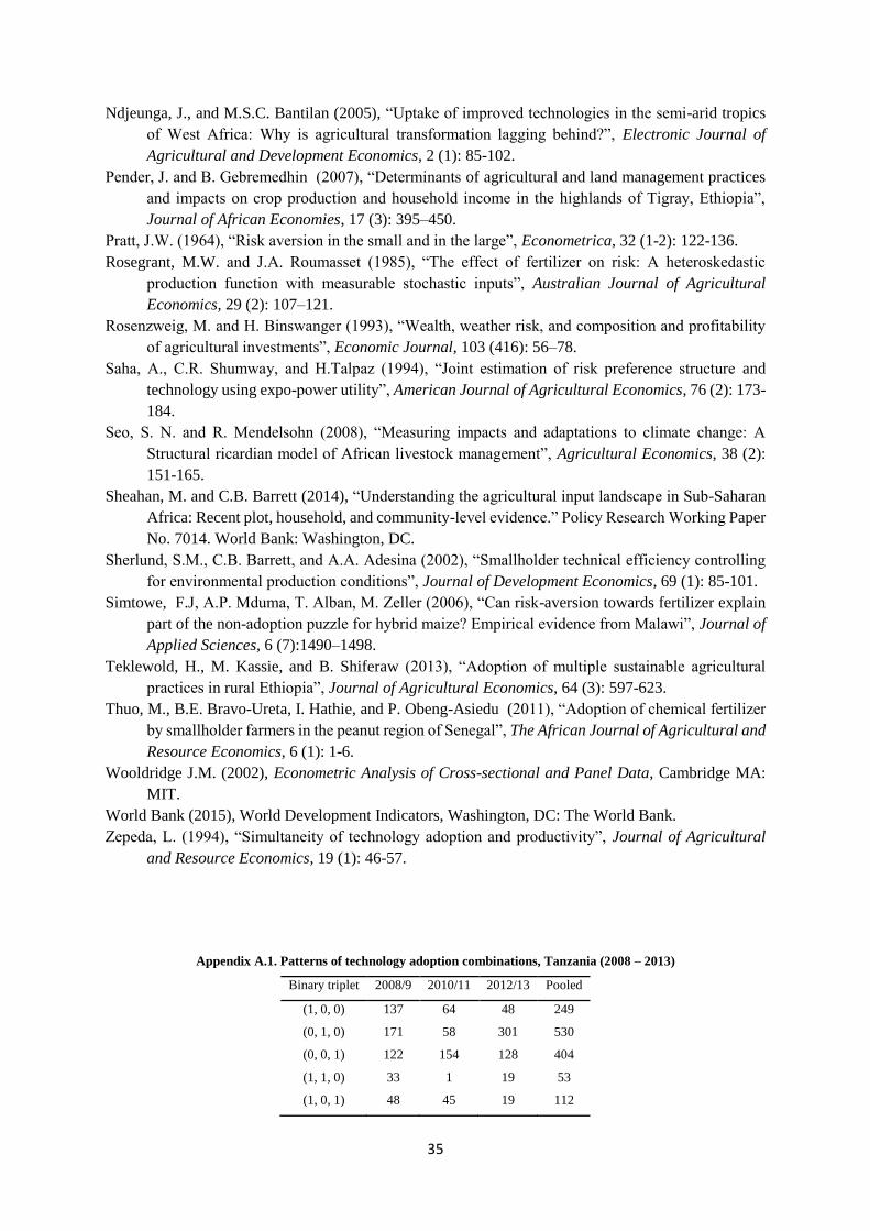
35

Ndjeunga, J., and M.S.C. Bantilan (2005), “Uptake of improved technologies in the semi-arid tropics

of West Africa: Why is agricultural transformation lagging behind?”, Electronic Journal of

Agricultural and Development Economics, 2 (1): 85-102.

Pender, J. and B. Gebremedhin (2007), “Determinants of agricultural and land management practices

and impacts on crop production and household income in the highlands of Tigray, Ethiopia”,

Journal of African Economies, 17 (3): 395–450.

Pratt, J.W. (1964), “Risk aversion in the small and in the large”, Econometrica, 32 (1-2): 122-136.

Rosegrant, M.W. and J.A. Roumasset (1985), “The effect of fertilizer on risk: A heteroskedastic

production function with measurable stochastic inputs”, Australian Journal of Agricultural

Economics, 29 (2): 107–121.

Rosenzweig, M. and H. Binswanger (1993), “Wealth, weather risk, and composition and profitability

of agricultural investments”, Economic Journal, 103 (416): 56–78.

Saha, A., C.R. Shumway, and H.Talpaz (1994), “Joint estimation of risk preference structure and

technology using expo-power utility”, American Journal of Agricultural Economics, 76 (2): 173-

184.

Seo, S. N. and R. Mendelsohn (2008), “Measuring impacts and adaptations to climate change: A

Structural ricardian model of African livestock management”, Agricultural Economics, 38 (2):

151-165.

Sheahan, M. and C.B. Barrett (2014), “Understanding the agricultural input landscape in Sub-Saharan

Africa: Recent plot, household, and community-level evidence.” Policy Research Working Paper

No. 7014. World Bank: Washington, DC.

Sherlund, S.M., C.B. Barrett, and A.A. Adesina (2002), “Smallholder technical efficiency controlling

for environmental production conditions”, Journal of Development Economics, 69 (1): 85-101.

Simtowe, F.J, A.P. Mduma, T. Alban, M. Zeller (2006), “Can risk-aversion towards fertilizer explain

part of the non-adoption puzzle for hybrid maize? Empirical evidence from Malawi”, Journal of

Applied Sciences, 6 (7):1490–1498.

Teklewold, H., M. Kassie, and B. Shiferaw (2013), “Adoption of multiple sustainable agricultural

practices in rural Ethiopia”, Journal of Agricultural Economics, 64 (3): 597-623.

Thuo, M., B.E. Bravo-Ureta, I. Hathie, and P. Obeng-Asiedu (2011), “Adoption of chemical fertilizer

by smallholder farmers in the peanut region of Senegal”, The African Journal of Agricultural and

Resource Economics, 6 (1): 1-6.

Wooldridge J.M. (2002), Econometric Analysis of Cross-sectional and Panel Data, Cambridge MA:

MIT.

World Bank (2015), World Development Indicators, Washington, DC: The World Bank.

Zepeda, L. (1994), “Simultaneity of technology adoption and productivity”, Journal of Agricultural

and Resource Economics, 19 (1): 46-57.

Appendix A.1. Patterns of technology adoption combinations, Tanzania (2008 – 2013)

Binary triplet 2008/9 2010/11 2012/13 Pooled

(1, 0, 0) 137 64 48 249

(0, 1, 0) 171 58 301 530

(0, 0, 1) 122 154 128 404

(1, 1, 0) 33 1 19 53

(1, 0, 1) 48 45 19 112

36

(0, 1, 1) 50 8 84 142

(1, 1, 1) 49 4 21 74

Total 610 334 620 1,564

Note: Each element in the triplet is a binary variable for the technology adoption combination Chemical fertilizer – Improved

seeds – Pesticide, having 1 if the specific input was applied by the farmer and 0 otherwise. The last row (“total”) gives

the total number of farmers that applied at least one of the three selected inputs. The number of farmers that did not

apply any of the selected modern inputs (the omitted category (0, 0, 0) can be obtained by the difference between the

sample size (2,158 per wave) and the above “total” row.

Appendix A.2. Patterns of technology adoption combinations, Uganda (2005 – 2012)

Binary triplet 2009/10 2010/11 2011/12 Pooled

(1, 0, 0) 7 10 20 37

(0, 1, 0) 314 211 312 837

(0, 0, 1) 98 120 99 317

(1, 1, 0) 24 8 18 50

(1, 0, 1) 13 13 18 44

37

(0, 1, 1) 82 65 77 224

(1, 1, 1) 33 32 35 100

Total 571 459 579 1,609

Note: Each element in the triplet is a binary variable for the technology adoption combination Chemical fertilizer – Improved

seeds – Pesticide, having 1 if the specific input was applied by the farmer and 0 otherwise. The last row (“total”) gives

the total number of farmers that applied at least one of the three selected inputs. The number of farmers that did not

apply any of the selected modern inputs (the omitted category (0, 0, 0) can be obtained by the difference between the

sample size (1,598 per wave) and the above “total” row.

Appendix A.3. Estimation of the flexible quadratic production function – Alternative specifications

Fixed effects models Mundlak-Chamberlain Fixed effects model

Variables Tanzania Uganda Tanzania Uganda

Coeffs Std errors Coeffs Std errors Coeffs Std errors Std errors Std errors

LAND 0.189 0.161 0.254*** 0.054 0.408*** 0.117 0.631** 0.315

LAND2 -0.045 0.061 0.154** 0.068 0.025 0.037 0.091*** 0.032

LABOR 2.250*** 0.188 0.119** 0.047 2.944*** 0.096 0.282** 0.051

LABOR2 -0.104*** 0.031 0.103** 0.048 -0.204*** 0.018 0.016 0.049

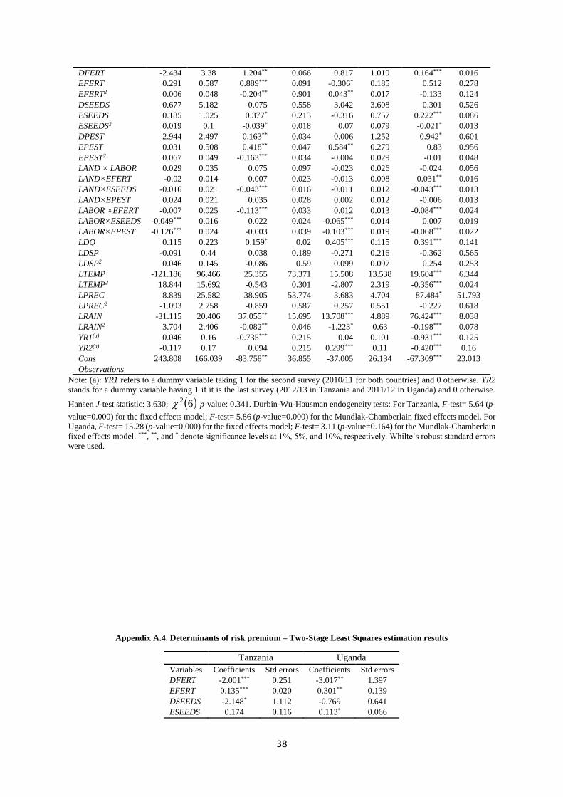
38

DFERT -2.434 3.38 1.204** 0.066 0.817 1.019 0.164*** 0.016

EFERT 0.291 0.587 0.889*** 0.091 -0.306* 0.185 0.512 0.278

EFERT2 0.006 0.048 -0.204** 0.901 0.043** 0.017 -0.133 0.124

DSEEDS 0.677 5.182 0.075 0.558 3.042 3.608 0.301 0.526

ESEEDS 0.185 1.025 0.377* 0.213 -0.316 0.757 0.222*** 0.086

ESEEDS2 0.019 0.1 -0.039* 0.018 0.07 0.079 -0.021* 0.013

DPEST 2.944 2.497 0.163** 0.034 0.006 1.252 0.942* 0.601

EPEST 0.031 0.508 0.418** 0.047 0.584** 0.279 0.83 0.956

EPEST2 0.067 0.049 -0.163*** 0.034 -0.004 0.029 -0.01 0.048

LAND × LABOR 0.029 0.035 0.075 0.097 -0.023 0.026 -0.024 0.056

LAND×EFERT -0.02 0.014 0.007 0.023 -0.013 0.008 0.031** 0.016

LAND×ESEEDS -0.016 0.021 -0.043*** 0.016 -0.011 0.012 -0.043*** 0.013

LAND×EPEST 0.024 0.021 0.035 0.028 0.002 0.012 -0.006 0.013

LABOR ×EFERT -0.007 0.025 -0.113*** 0.033 0.012 0.013 -0.084*** 0.024

LABOR×ESEEDS -0.049*** 0.016 0.022 0.024 -0.065*** 0.014 0.007 0.019

LABOR×EPEST -0.126*** 0.024 -0.003 0.039 -0.103*** 0.019 -0.068*** 0.022

LDQ 0.115 0.223 0.159* 0.02 0.405*** 0.115 0.391*** 0.141

LDSP -0.091 0.44 0.038 0.189 -0.271 0.216 -0.362 0.565

LDSP2 0.046 0.145 -0.086 0.59 0.099 0.097 0.254 0.253

LTEMP -121.186 96.466 25.355 73.371 15.508 13.538 19.604*** 6.344

LTEMP2 18.844 15.692 -0.543 0.301 -2.807 2.319 -0.356*** 0.024

LPREC 8.839 25.582 38.905 53.774 -3.683 4.704 87.484* 51.793

LPREC2 -1.093 2.758 -0.859 0.587 0.257 0.551 -0.227 0.618

LRAIN -31.115 20.406 37.055** 15.695 13.708*** 4.889 76.424*** 8.038

LRAIN2 3.704 2.406 -0.082** 0.046 -1.223* 0.63 -0.198*** 0.078

YR1(a) 0.046 0.16 -0.735*** 0.215 0.04 0.101 -0.931*** 0.125

YR2(a) -0.117 0.17 0.094 0.215 0.299*** 0.11 -0.420*** 0.16

Cons 243.808 166.039 -83.758** 36.855 -37.005 26.134 -67.309*** 23.013

Observations

Note: (a): YR1 refers to a dummy variable taking 1 for the second survey (2010/11 for both countries) and 0 otherwise. YR2

stands for a dummy variable having 1 if it is the last survey (2012/13 in Tanzania and 2011/12 in Uganda) and 0 otherwise.

Hansen J-test statistic: 3.630; 62 p-value: 0.341. Durbin-Wu-Hausman endogeneity tests: For Tanzania, F-test= 5.64 (p-

value=0.000) for the fixed effects model; F-test= 5.86 (p-value=0.000) for the Mundlak-Chamberlain fixed effects model. For

Uganda, F-test= 15.28 (p-value=0.000) for the fixed effects model; F-test= 3.11 (p-value=0.164) for the Mundlak-Chamberlain

fixed effects model. ***, **, and * denote significance levels at 1%, 5%, and 10%, respectively. Whilte’s robust standard errors

were used.

Appendix A.4. Determinants of risk premium – Two-Stage Least Squares estimation results

Tanzania Uganda

Variables Coefficients Std errors Coefficients Std errors

DFERT -2.001*** 0.251 -3.017** 1.397

EFERT 0.135*** 0.020 0.301** 0.139

DSEEDS -2.148* 1.112 -0.769 0.641

ESEEDS 0.174 0.116 0.113* 0.066

39

DPEST -0.147** 0.073 -4.785*** 0.602

EPEST 0.010** 0.004 0.554*** 0.070

LAND -0.038*** 0.003 -0.024** 0.010

LABOR -0.094*** 0.011 -0.257*** 0.023

LDQ 0.071 0.055 0.047 0.033

LDIR 0.136 0.115 0.095 0.087

LDSP 0.000 0.077 -0.126** 0.059

AGE -0.003*** 0.000 -0.002 0.004

GENDER 0.127*** 0.012 0.015 0.099

HHSIZE 0.028 0.022 -0.076*** 0.018

EDUC -0.004** 0.002 -0.003 0.008

Obs. 4,316 3,196

Note: Robust standard errors are reported. ***, **, and * indicate statistical significance at the 1, 5, and 10% levels, respectively.

Recent Publications in the Series

nº Year Author(s) Title

232 2015 Linguère Mously Mbaye Remittances and Access to Rural Credit Markets: Evidence from

Senegal

231 2015 Adamon N. Mukasa and Adeleke O.

Salami

Gender productivity differentials among smallholder farmers in

Africa: A cross-country comparison

230 2015 Valérie Bérenger and Audrey Verdier-

Chouchane

Child Labour and Schooling in South Sudan and Sudan:

Is There a Gender Preference?

229 2015 Luc Christiaensen and Jonathan Kaminski Structural change, economic growth and poverty reduction –

Micro-evidence from Uganda

228 2015 Mouhamadou Sy Overborrowing and Balance of Payments Imbalances in a

Monetary Union

227 2015 Mthuli Ncube and Zuzana Brixiová Public Debt Sustainability in Africa: Building Resilience and

Challenges Ahead

226 2015 Elphas Ojiambo, Jacob Oduor, Tom

Mburu and Nelson Wawire Aid Unpredictability and Economic Growth in Kenya

225 2015 Andinet Woldemichael and Abebe

Shimeles

Measuring the Impact of Micro-Health Insurance on Healthcare

Utilization: A Bayesian Potential Outcomes Approach

224 2015 Gibert Galibaka Sophistication of Fruits, Vegetables and Derivatives Exports in

the WAEMU space

223 2015 Zorobabel Bicaba, Zuzana Brixiová and

Mthuli Ncube

Extreme Poverty in Africa: Trends, Policies and the Role of

International Organizations