tecnología y estructura de costos
DESCRIPTION
Tecnología y Estructura de Costos. Technologies. A technology is a process by which inputs are converted to an output. E.g. labor, a computer, a projector, electricity, and software are being combined to produce this lecture. Technologies. - PowerPoint PPT PresentationTRANSCRIPT
Tecnología y Estructura de Costos
Technologies
A technology is a process by which inputs are converted to an output.
E.g. labor, a computer, a projector, electricity, and software are being combined to produce this lecture.

Technologies
Usually several technologies will produce the same product -- a blackboard and chalk can be used instead of a computer and a projector.
Which technology is “best”? How do we compare technologies?
Input Bundles
xi denotes the amount used of input i; i.e. the level of input i.
An input bundle is a vector of the input levels; (x1, x2, … , xn).
E.g. (x1, x2, x3) = (6, 0, 93).
Production Functions
y denotes the output level. The technology’s production
function states the maximum amount of output possible from an input bundle.
y f x xn ( , , )1
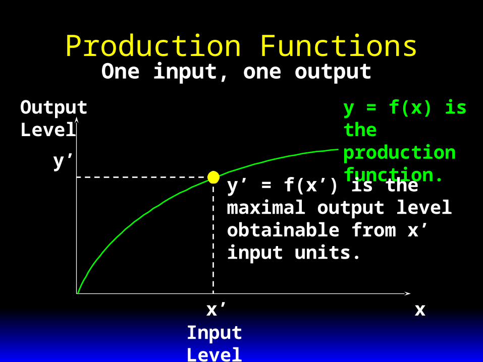
Production Functions
y = f(x) is theproductionfunction.
x’ xInput Level
Output Level
y’y’ = f(x’) is the maximal output level obtainable from x’ input units.
One input, one output
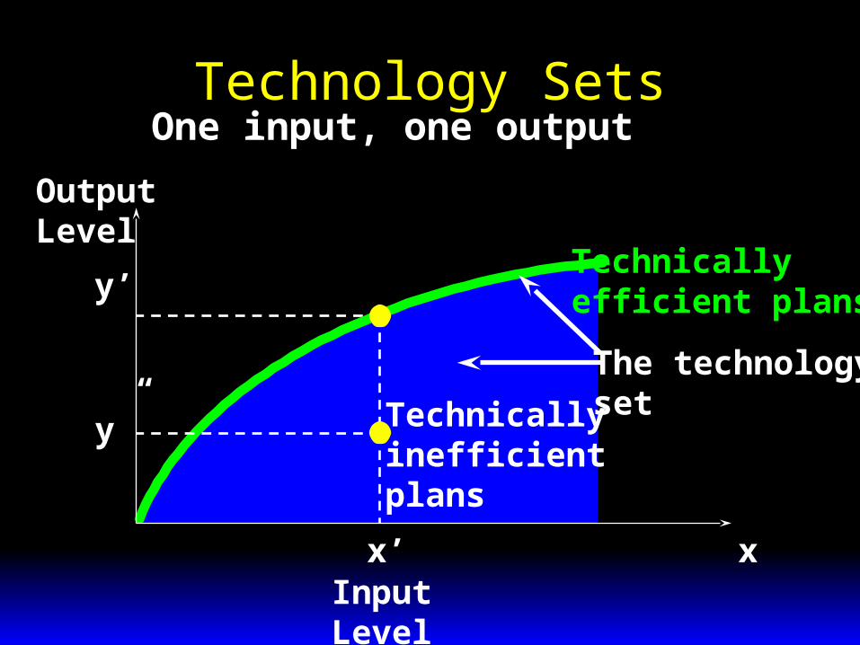
Technology Sets
A production plan is an input bundle and an output level; (x1, … , xn, y).
The collection of all feasible
production plans is the technology set.
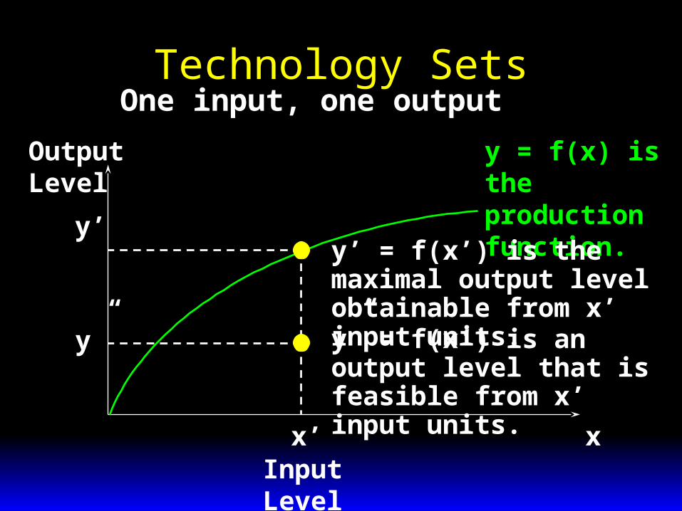
Technology Sets
y = f(x) is theproductionfunction.
x’ xInput Level
Output Level
y’
y”
y’ = f(x’) is the maximal output level obtainable from x’ input units.
One input, one output
y” = f(x’) is an output level that is feasible from x’ input units.
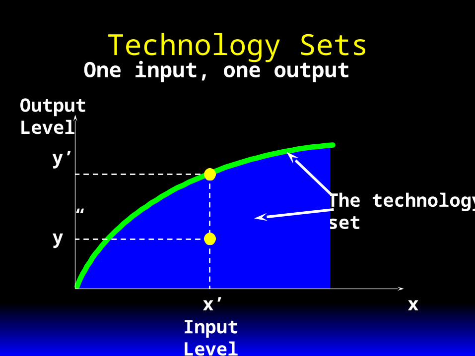
Technology Sets
x’ xInput Level
Output Level
y’
One input, one output
y”
The technologyset
Technology Sets
x’ xInput Level
Output Level
y’
One input, one output
y”
The technologysetTechnically
inefficientplans
Technicallyefficient plans
Technologies with Multiple Inputs
What does a technology look like when there is more than one input?
The two input case: Input levels are x1 and x2. Output level is y.
Suppose the production function is
y f x x x x ( , ) .1 2 11/3
21/32
Technologies with Multiple Inputs
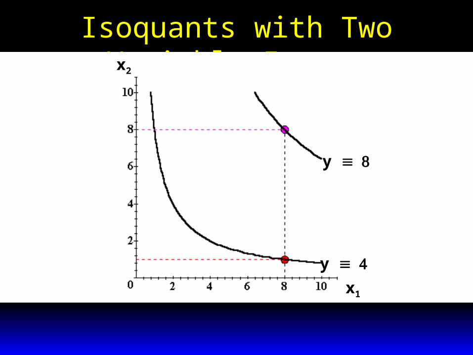
E.g. the maximal output level possible from the input bundle(x1, x2) = (1, 8) is
And the maximal output level possible from (x1,x2) = (8,8) is
y x x 2 2 1 8 2 1 2 411/3
21/3 1/3 1/3 .
y x x 2 2 8 8 2 2 2 811/3
21/3 1/3 1/3 .
Technologies with Multiple Inputs
The y output unit isoquant is the set of all input bundles that yield at most the same output level y.
Isoquants with Two Variable Inputs
y
y x1
x2

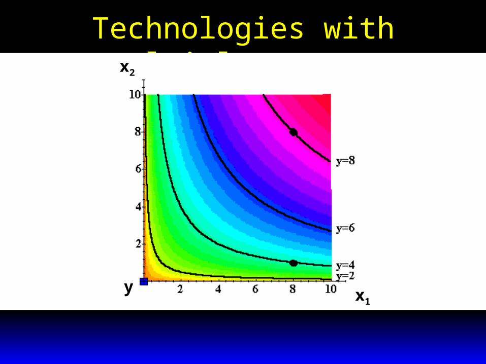
Technologies with Multiple Inputs
The complete collection of isoquants is the isoquant map.
The isoquant map is equivalent to the production function -- each is the other.
E.g. 3/12
3/1121 2),( xxxxfy
Technologies with Multiple Inputs
x1
x2
y

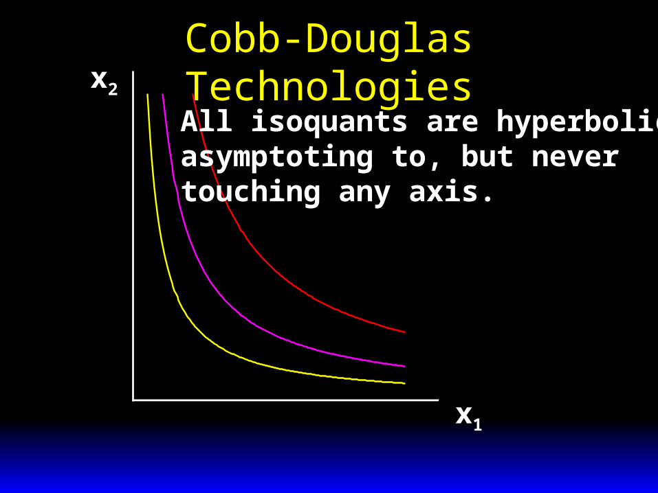
Cobb-Douglas Technologies
A Cobb-Douglas production function is of the form
E.g.
with
y Ax x xa anan 1 2
1 2 .
y x x 11/3
21/3
n A a and a 2 113
131 2, , .
x2
x1
All isoquants are hyperbolic,asymptoting to, but nevertouching any axis.
Cobb-Douglas Technologies
y x xa a 1 21 2

x2
x1
All isoquants are hyperbolic,asymptoting to, but nevertouching any axis.
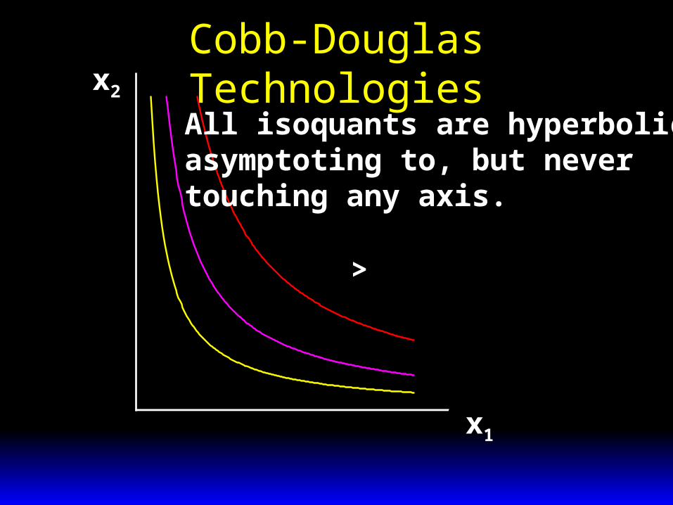
Cobb-Douglas Technologies
x x ya a1 2
1 2 "
y x xa a 1 21 2

x2
x1
All isoquants are hyperbolic,asymptoting to, but nevertouching any axis.
Cobb-Douglas Technologies
x x ya a1 2
1 2 '
x x ya a1 2
1 2 "
y x xa a 1 21 2
x2
x1
All isoquants are hyperbolic,asymptoting to, but nevertouching any axis.
Cobb-Douglas Technologies
x x ya a1 2
1 2 '
x x ya a1 2
1 2 "
y" y'>y x xa a 1 2
1 2
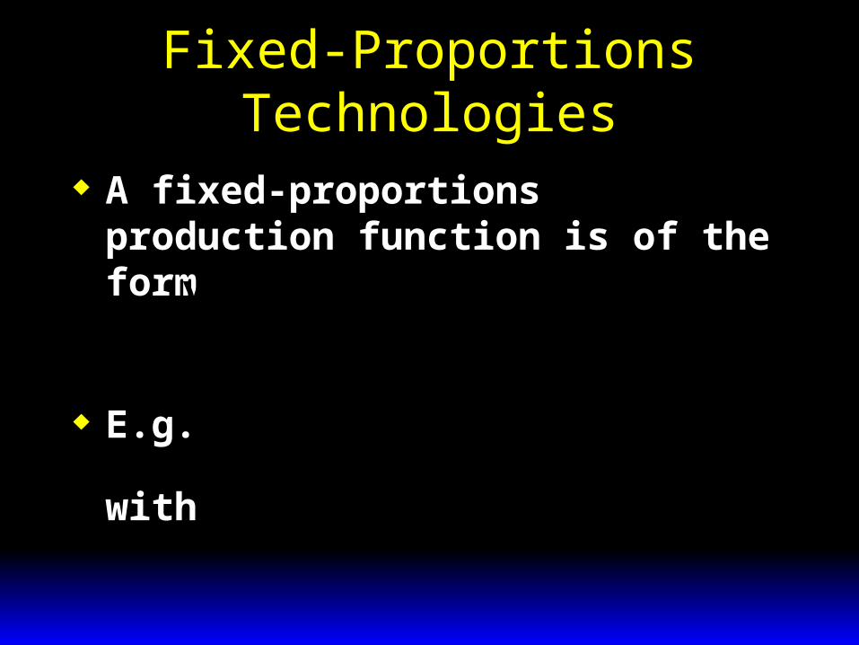
Fixed-Proportions Technologies
A fixed-proportions production function is of the form
E.g.
with
y a x a x a xn nmin{ , , , }.1 1 2 2
y x xmin{ , }1 22
n a and a 2 1 21 2, .
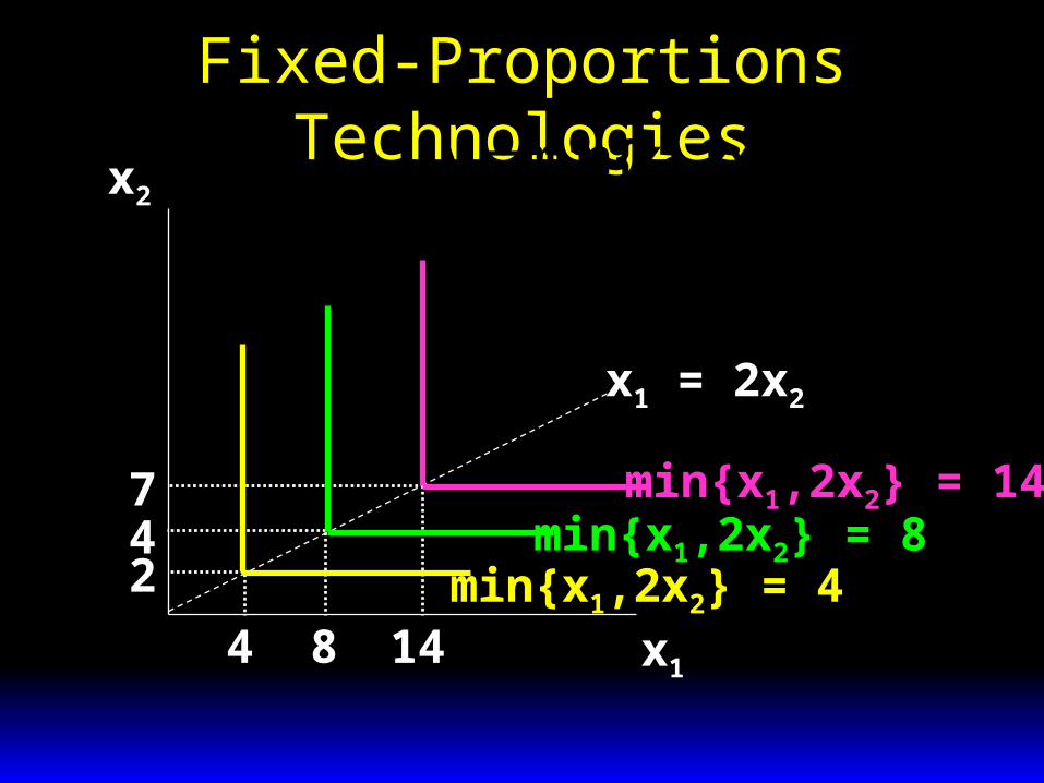
Fixed-Proportions Technologiesx2
x1
min{x1,2x2} = 14
4 8 14
247
min{x1,2x2} = 8min{x1,2x2} = 4
x1 = 2x2
y x xmin{ , }1 22
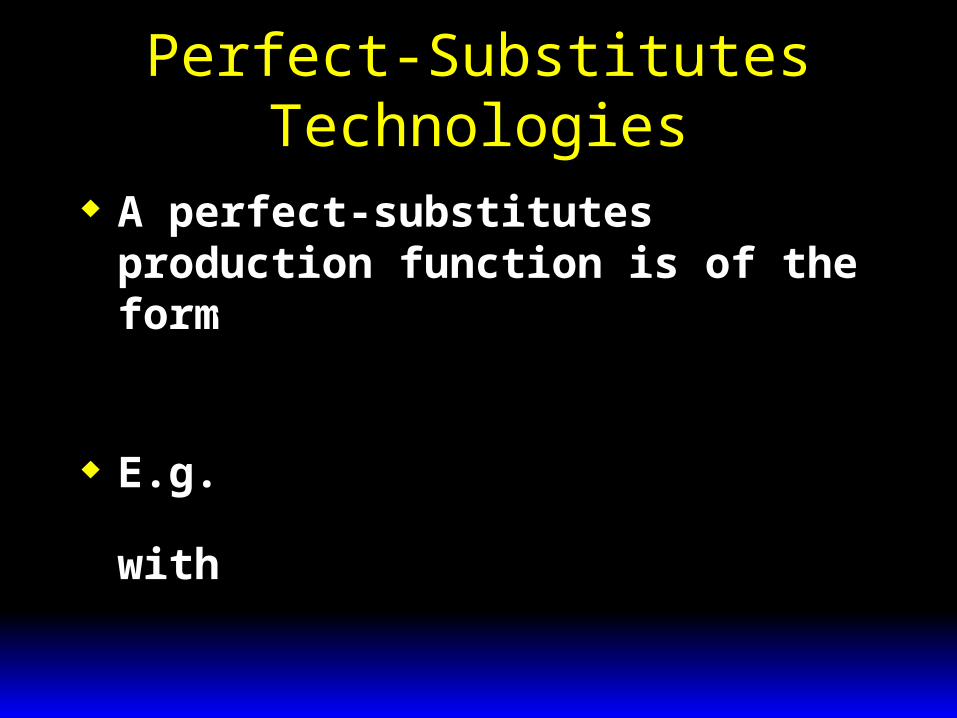
Perfect-Substitutes Technologies
A perfect-substitutes production function is of the form
E.g.
with
y a x a x a xn n 1 1 2 2 .
y x x 1 23
n a and a 2 1 31 2, .

Perfect-Substitution Technologies
9
3
18
6
24
8
x1
x2
x1 + 3x2 = 18
x1 + 3x2 = 36
x1 + 3x2 = 48
All are linear and parallel
y x x 1 23
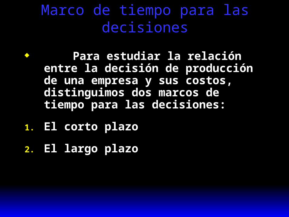
Marco de tiempo para las decisiones
Para estudiar la relación entre la decisión de producción de una empresa y sus costos, distinguimos dos marcos de tiempo para las decisiones:
1. El corto plazo
2. El largo plazo
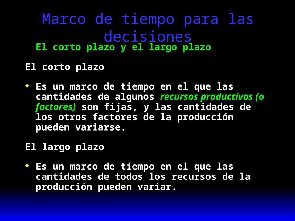
Marco de tiempo para las decisionesEl corto plazo y el largo plazo
El corto plazo
Es un marco de tiempo en el que las cantidades de algunos recursos productivos (o factores) son fijas, y las cantidades de los otros factores de la producción pueden variarse.
El largo plazo
Es un marco de tiempo en el que las cantidades de todos los recursos de la producción pueden variar.
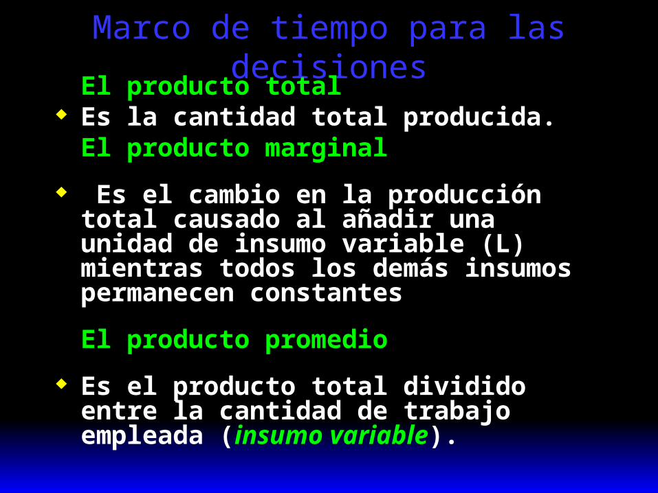
Marco de tiempo para las decisionesEl producto total
Es la cantidad total producida.El producto marginal
Es el cambio en la producción total causado al añadir una unidad de insumo variable (L) mientras todos los demás insumos permanecen constantes
El producto promedio
Es el producto total dividido entre la cantidad de trabajo empleada (insumo variable).
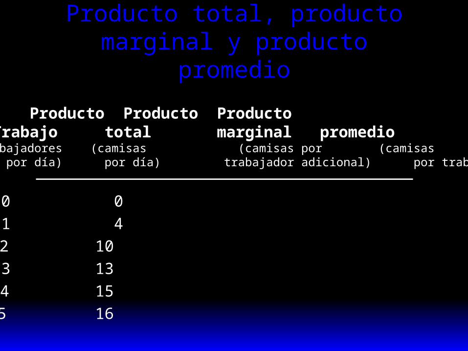
Producto total, producto marginal y producto promedio
Producto Producto Producto Trabajo total marginal promedio (trabajadores (camisas (camisas por (camisas por día) por día) trabajador adicional) por trabajador)
a 0 0
b 1 4
c 2 10
d 3 13
e 4 15
f 5 16
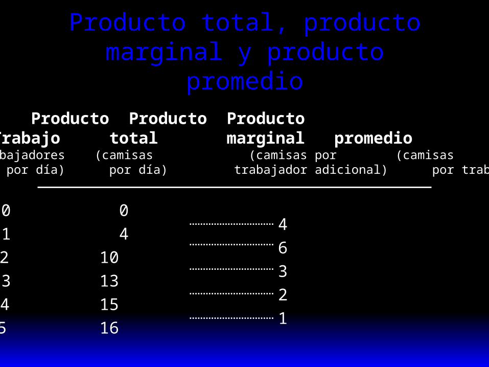
Producto total, producto marginal y producto promedio
Producto Producto Producto Trabajo total marginal promedio (trabajadores (camisas (camisas por (camisas por día) por día) trabajador adicional) por trabajador)
a 0 0
b 1 4
c 2 10
d 3 13
e 4 15
f 5 16
4
6
3
2
1
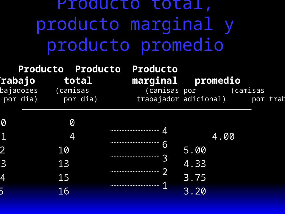
Producto total, producto marginal y producto promedio
Producto Producto Producto Trabajo total marginal promedio (trabajadores (camisas (camisas por (camisas por día) por día) trabajador adicional) por trabajador)
a 0 0
b 1 4 4.00
c 2 10 5.00
d 3 13 4.33
e 4 15 3.75
f 5 16 3.20
4
6
3
2
1
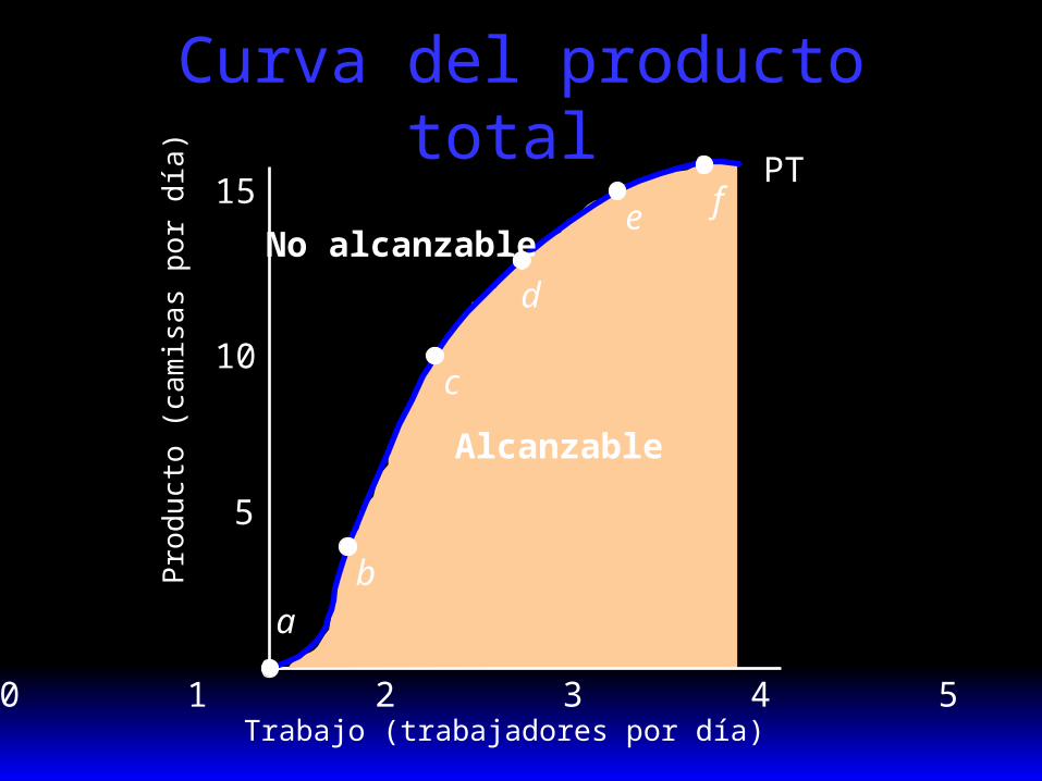
Alcanzable
Curva del producto total
0 1 2 3 4 5Trabajo (trabajadores por día)
5
10
15PT
No alcanzable
Pro
duct
o (c
amis
as p
or d
ía)
a
b
c
d
e f
Curva del producto marginal El producto marginal se mide también por
la pendiente de la curva del producto total.
Ley de los rendimientos decrecientes
Principio que afirma que más alla de cierto punto el producto marginal disminuye a medida que se agregan unidades adicionales de un factor variable a un factor fijo.
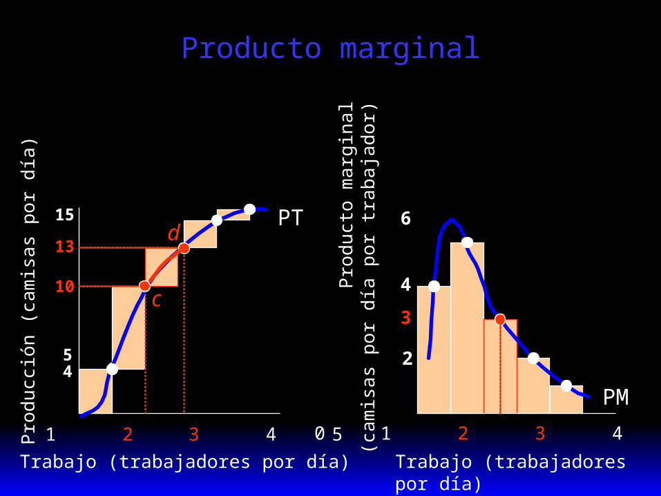
Producto marginal
0 1 2 3 4 5
Trabajo (trabajadores por día)
5
10
15 PT
Pro
ducc
ión
(cam
isas
por
día
)
0 1 2 3 4 5
Trabajo (trabajadores por día)
2
4
6
Pro
duct
o m
argi
nal
(cam
isas
por
día
por
trab
ajad
or)
4
3
13
PM
c
d
Marginal (Physical) Products
The marginal product of input i is the rate-of-change of the output level as the level of input i changes, holding all other input levels fixed.
That is,
y f x xn ( , , )1
ii x
yMP
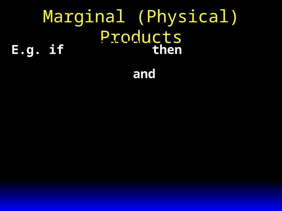
Marginal (Physical) ProductsE.g. if
y f x x x x ( , ) /1 2 1
1/322 3
then the marginal product of input 1 is

Marginal (Physical) ProductsE.g. if
y f x x x x ( , ) /1 2 1
1/322 3
then the marginal product of input 1 is
MPyx
x x11
12 3
22 31
3
/ /
Marginal (Physical) ProductsE.g. if
y f x x x x ( , ) /1 2 1
1/322 3
then the marginal product of input 1 is
MPyx
x x11
12 3
22 31
3
/ /
and the marginal product of input 2 is

Marginal (Physical) ProductsE.g. if
y f x x x x ( , ) /1 2 1
1/322 3
then the marginal product of input 1 is
MPyx
x x11
12 3
22 31
3
/ /
and the marginal product of input 2 is
MPy
xx x2
211/3
21/32
3
.
Marginal (Physical) Products
The marginal product of input i is diminishing if it becomes smaller as the level of input i increases. That is, if
.02
2
iiii
i
x
y
x
y
xx
MP
Marginal (Physical) Products
MP x x1 12 3
22 31
3 / / MP x x2 1
1/32
1/323
and
E.g. if y x x 11/3
22 3/ then
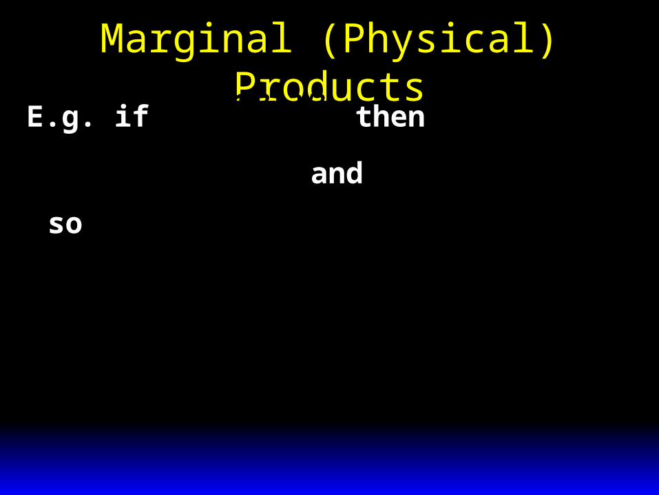
Marginal (Physical) Products
MP x x1 12 3
22 31
3 / / MP x x2 1
1/32
1/323
and
so MPx
x x1
11
5 322 32
90 / /
E.g. if y x x 11/3
22 3/ then
Marginal (Physical) Products
MP x x1 12 3
22 31
3 / / MP x x2 1
1/32
1/323
and
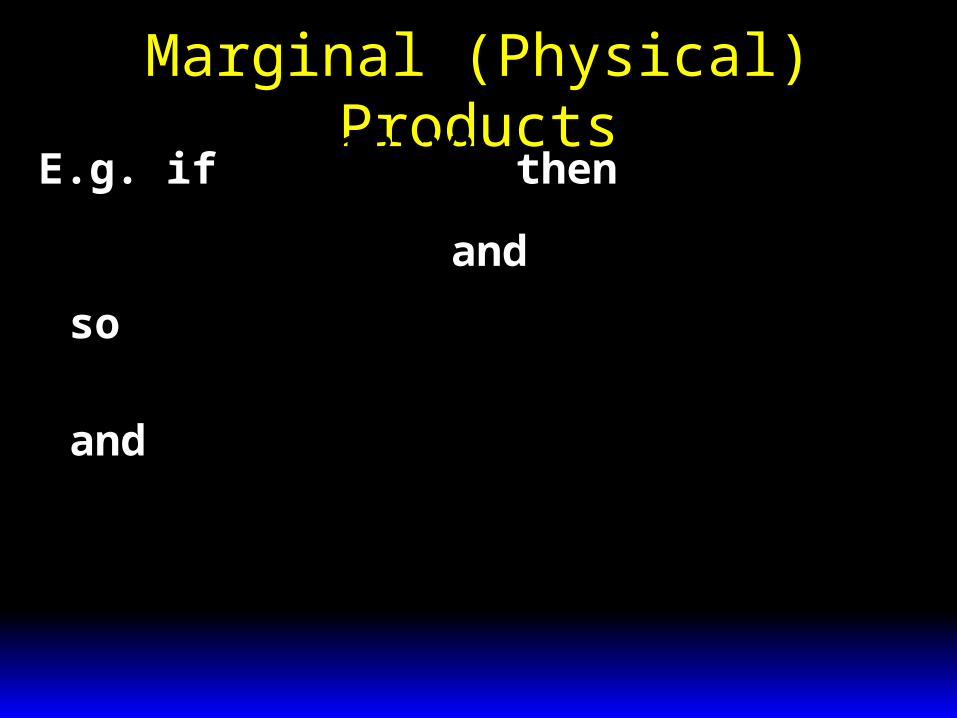
so MPx
x x1
11
5 322 32
90 / /
MPx
x x2
211/3
24 32
90 / .
and
E.g. if y x x 11/3
22 3/ then
Marginal (Physical) Products
MP x x1 12 3
22 31
3 / / MP x x2 1
1/32
1/323
and
so MPx
x x1
11
5 322 32
90 / /
MPx
x x2
211/3
24 32
90 / .
and
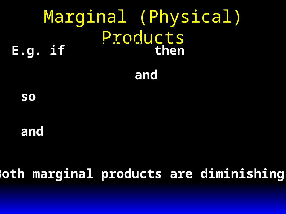
Both marginal products are diminishing.
E.g. if y x x 11/3
22 3/ then
Returns-to-Scale
Returns-to-scale describes how the output level changes as all input levels change in direct proportion (e.g. all input levels doubled, or halved).
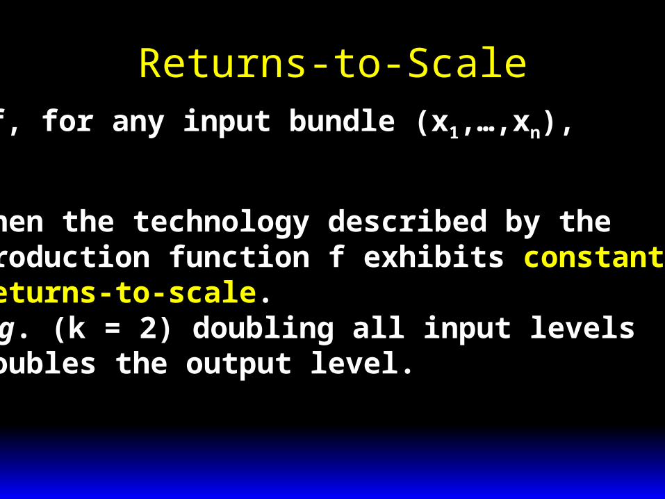
Returns-to-ScaleIf, for any input bundle (x1,…,xn),
f kx kx kx kf x x xn n( , , , ) ( , , , )1 2 1 2
then the technology described by theproduction function f exhibits constantreturns-to-scale.E.g. (k = 2) doubling all input levelsdoubles the output level.
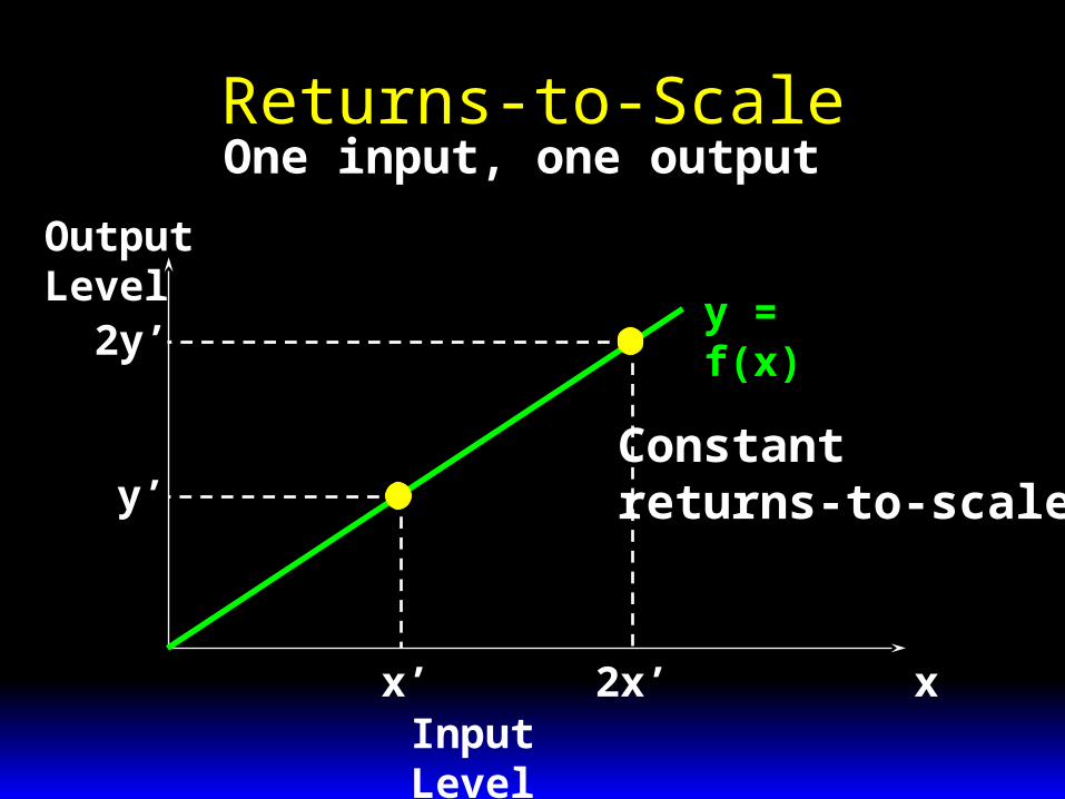
Returns-to-Scale
y = f(x)
x’ xInput Level
Output Level
y’
One input, one output
2x’
2y’
Constantreturns-to-scale
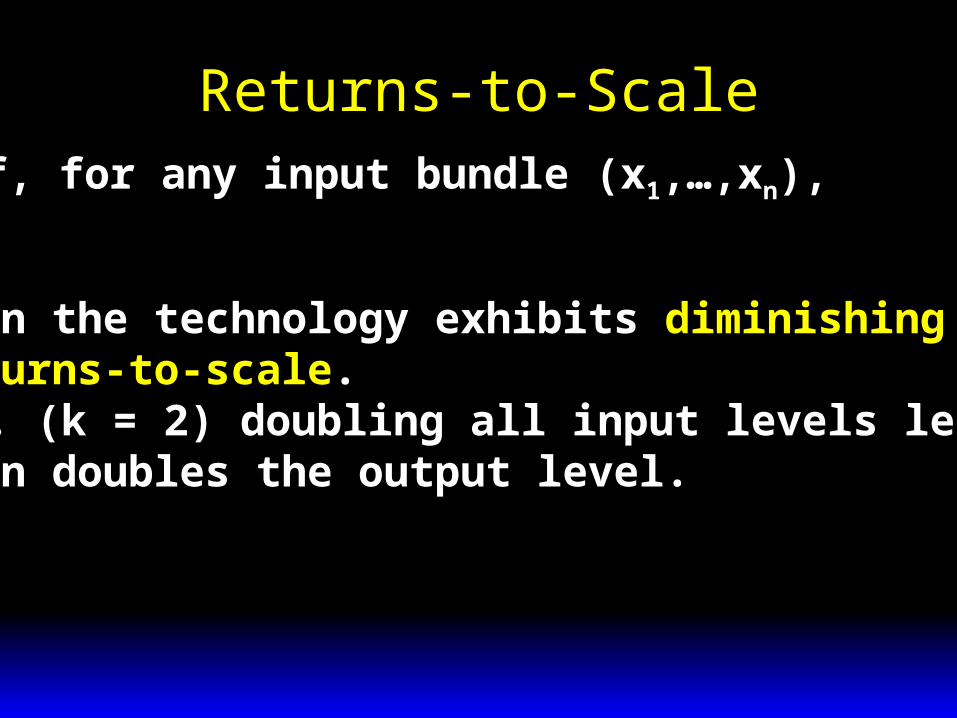
Returns-to-ScaleIf, for any input bundle (x1,…,xn),
f kx kx kx kf x x xn n( , , , ) ( , , , )1 2 1 2
then the technology exhibits diminishingreturns-to-scale.E.g. (k = 2) doubling all input levels less than doubles the output level.
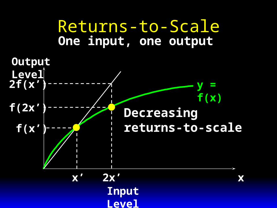
Returns-to-Scale
y = f(x)
x’ xInput Level
Output Level
f(x’)
One input, one output
2x’
f(2x’)
2f(x’)
Decreasingreturns-to-scale
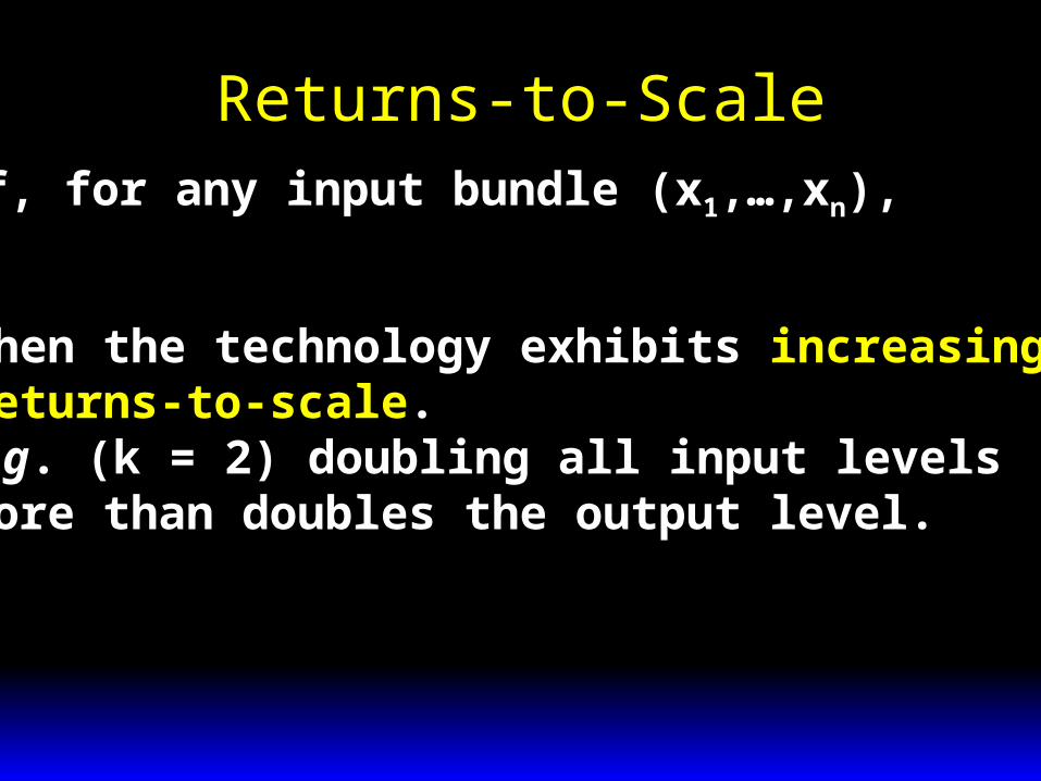
Returns-to-ScaleIf, for any input bundle (x1,…,xn),
f kx kx kx kf x x xn n( , , , ) ( , , , )1 2 1 2
then the technology exhibits increasingreturns-to-scale.E.g. (k = 2) doubling all input levelsmore than doubles the output level.

Returns-to-Scale
y = f(x)
x’ xInput Level
Output Level
f(x’)
One input, one output
2x’
f(2x’)
2f(x’)
Increasingreturns-to-scale