temperature as a function of depth and time paul evans ...topex.ucsd.edu/.../c_wine_cellar.pdf ·...
TRANSCRIPT

Temperature as a function of depth and time
Paul Evans & Christine WittichSIO234: Geodynamics, Prof. Sandwell
Fall 2011

Periodic Heating of the Surface of the Earth Why is it the wine cellar problem?
Wine ages best when kept at a constant temperature If we understand the heating that occurs at the surface of
the Earth, we can choose an appropriate cellar depthOther Applications Geodynamics
Determine diffusivity, , of rocks and soil Structural Engineering
Determine required foundation depth to prevent heaving


Defining the Problem
x
z
TS
Earth
Atmosphere
FIND: T (z , t)
Note:

Solving for T (z, t)
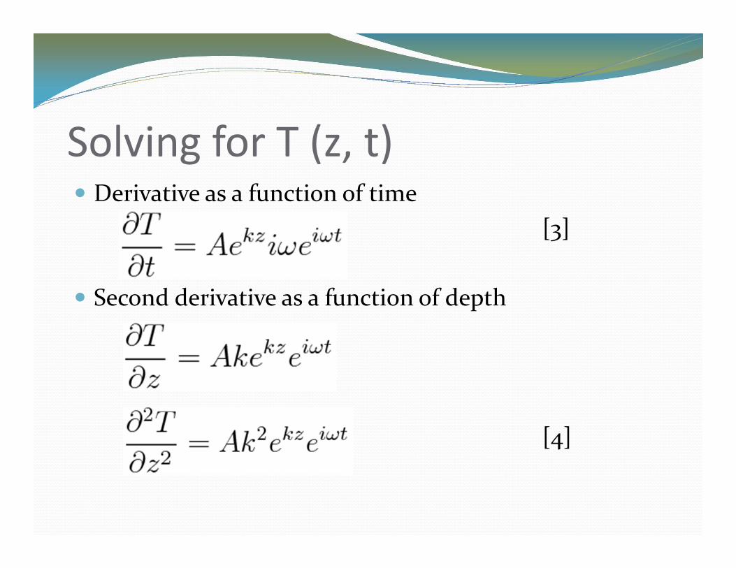
Solving for T (z, t) Derivative as a function of time
[3]
Second derivative as a function of depth
[4]
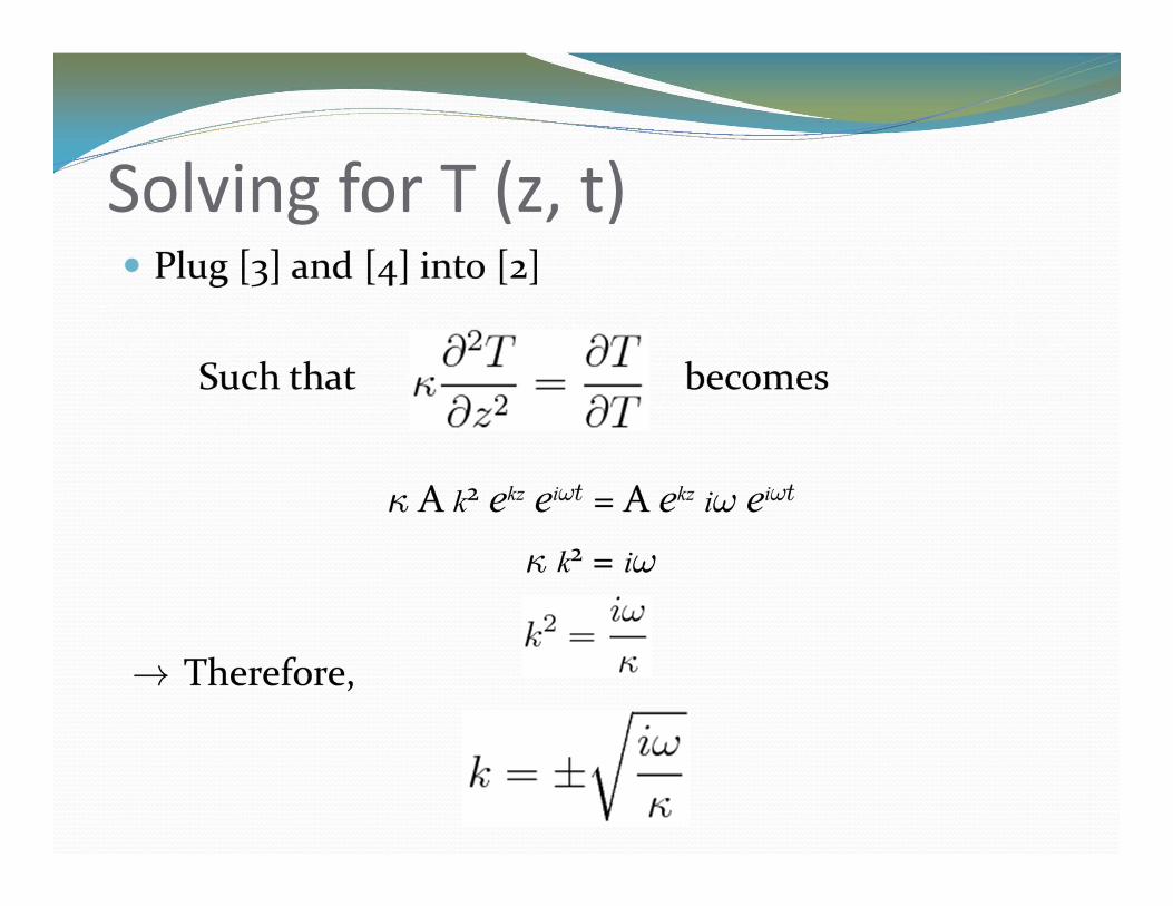
Solving for T (z, t)
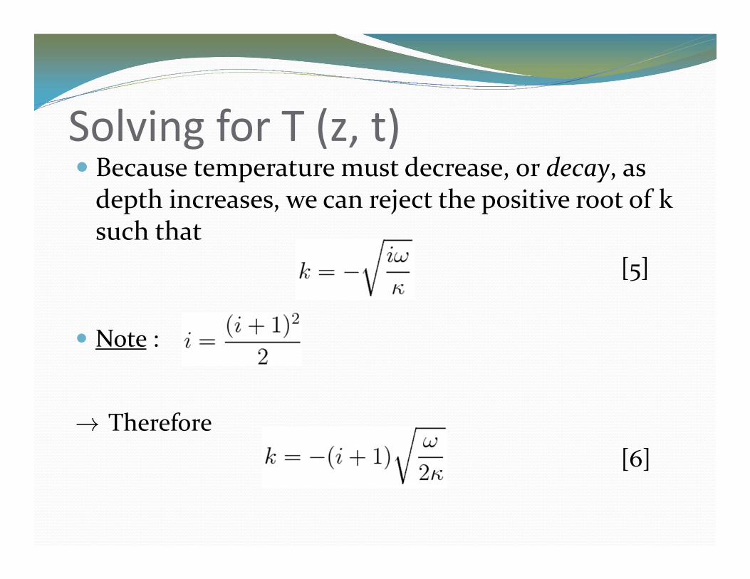
Solving for T (z, t) Because temperature must decrease, or decay, as
depth increases, we can reject the positive root of k such that
[5]
Note :
→ Therefore [6]
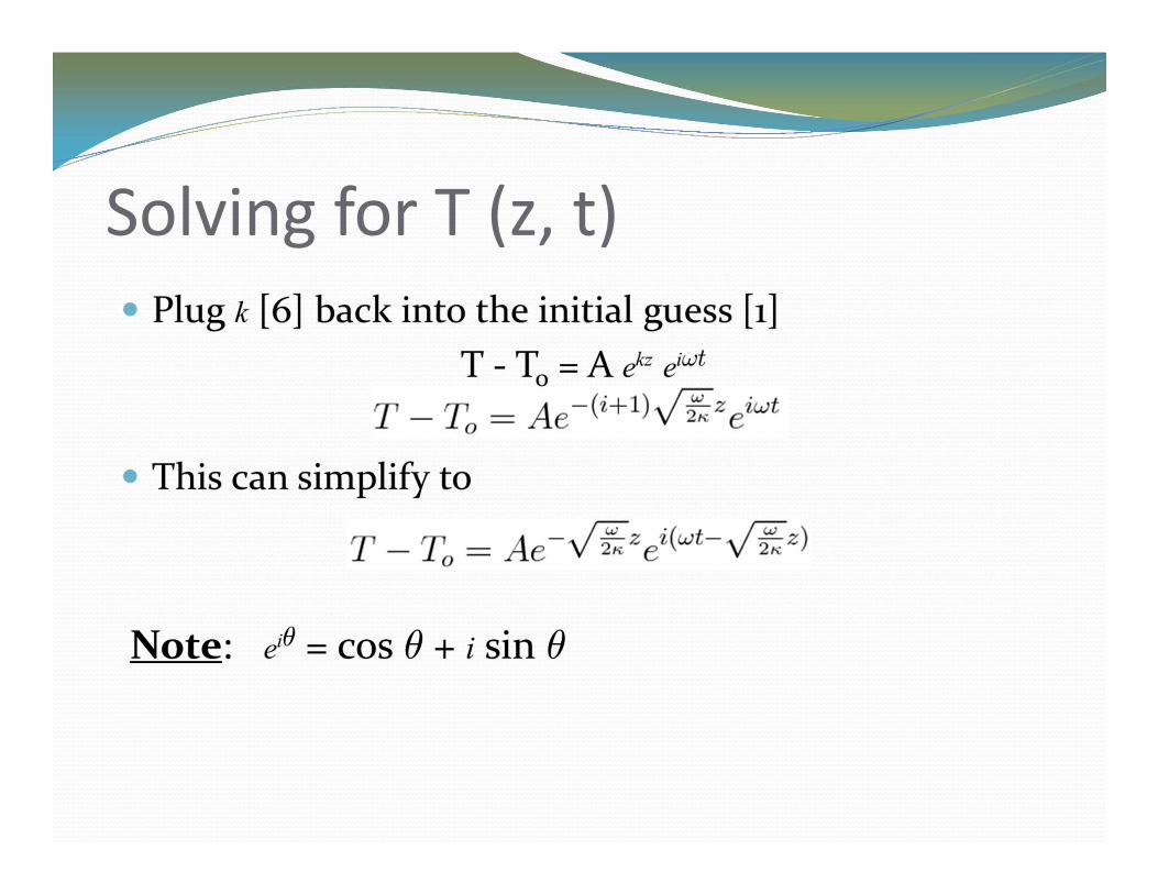
Solving for T (z, t)

Solving for T (z, t)

Solving for T (z, t)

Solving for T (z, t) Using boundary condition of T(0, t) = TS
The temperature variation in the Earth due the periodic surface temperatures is
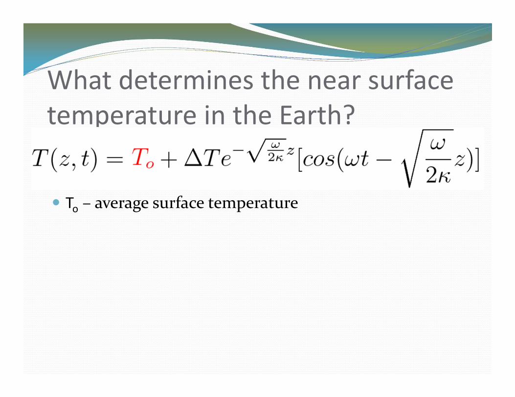
What determines the near surface temperature in the Earth?
To – average surface temperature

What determines the near surface temperature in the Earth?
To – average surface temperature – ½ total temperature range (amplitude)
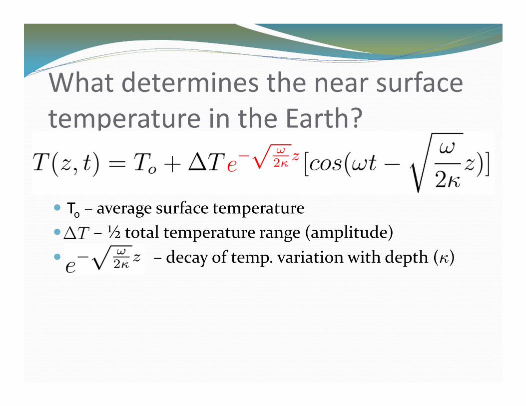
What determines the near surface temperature in the Earth?
To – average surface temperature – ½ total temperature range (amplitude) – decay of temp. variation with depth (κ)

What determines the near surface temperature in the Earth?
To – average surface temperature – ½ total temperature range (amplitude) – decay of temp. variation with depth (κ)
cosine – periodic change in temperature

What determines the near surface temperature in the Earth?
To – average surface temperature – ½ total temperature range (amplitude) – decay of temp. variation with depth (κ)
cosine – periodic change in temperature
– phase shift due to time lag betweensurface temp. and temp. at depth z

How deep do we put a wine cellar? Wine cellar should be put at a depth where
temperature fluctuations due to periodic surface changes will be minimal
Apply concept of skin depth
Skin Depth, zo depth at which temperature fluctuation is 1/e of the surface
temperature fluctuation 1/e ≈ 0.37, which therefore represents a 63% reduction in
temperature fluctuation
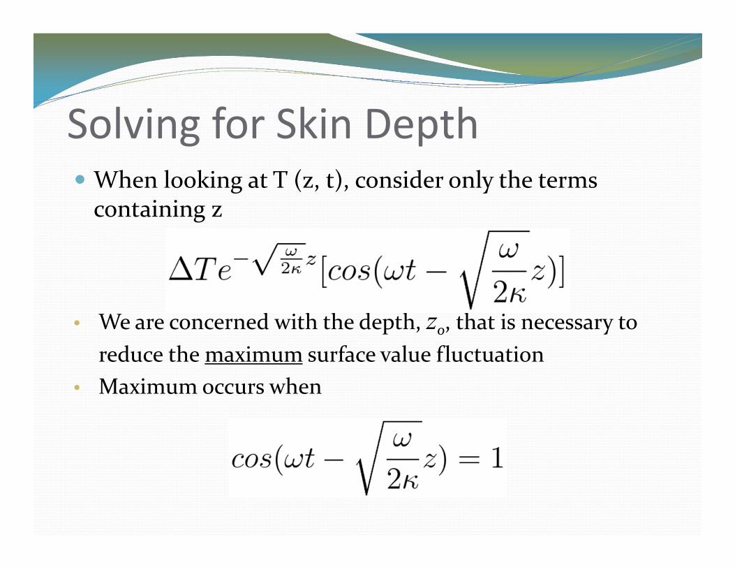
Solving for Skin Depth When looking at T (z, t), consider only the terms
containing z
• We are concerned with the depth, zo, that is necessary to reduce the maximum surface value fluctuation
• Maximum occurs when

Solving for Skin Depth To determine zo, set
Note: The depth zo can easily be adjusted to represent a different reduction in surface temperature fluctuation by replacing 1/e with the desired value
i.e. – replace 1/e with 0.10 for depth at which 90% reduction occurs
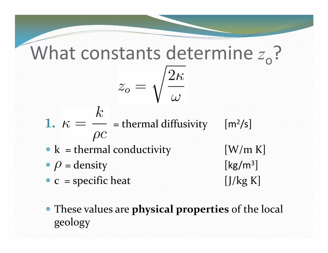
What constants determine zo?
1. = thermal diffusivity [m2/s]
k = thermal conductivity [W/m K] = density [kg/m3] c = specific heat [J/kg K]
These values are physical properties of the local geology

What constants determine zo?
2. = circular frequency
Recall and = period of concern [sec] varies depending on what time scale is of
concern
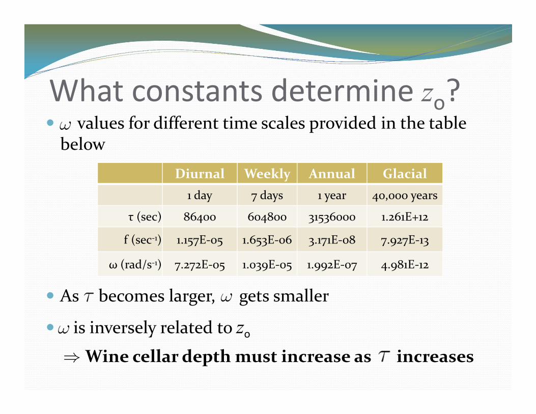
What constants determine zo? values for different time scales provided in the table
below
As becomes larger, gets smaller
is inversely related to zo⇒ Wine cellar depth must increase as increases
Diurnal Weekly Annual Glacial1 day 7 days 1 year 40,000 years
τ (sec) 86400 604800 31536000 1.261E+12
f (sec-1) 1.157E-05 1.653E-06 3.171E-08 7.927E-13
ω (rad/s-1) 7.272E-05 1.039E-05 1.992E-07 4.981E-12

Simplified T (z, t) By substituting zo into T (z, t)
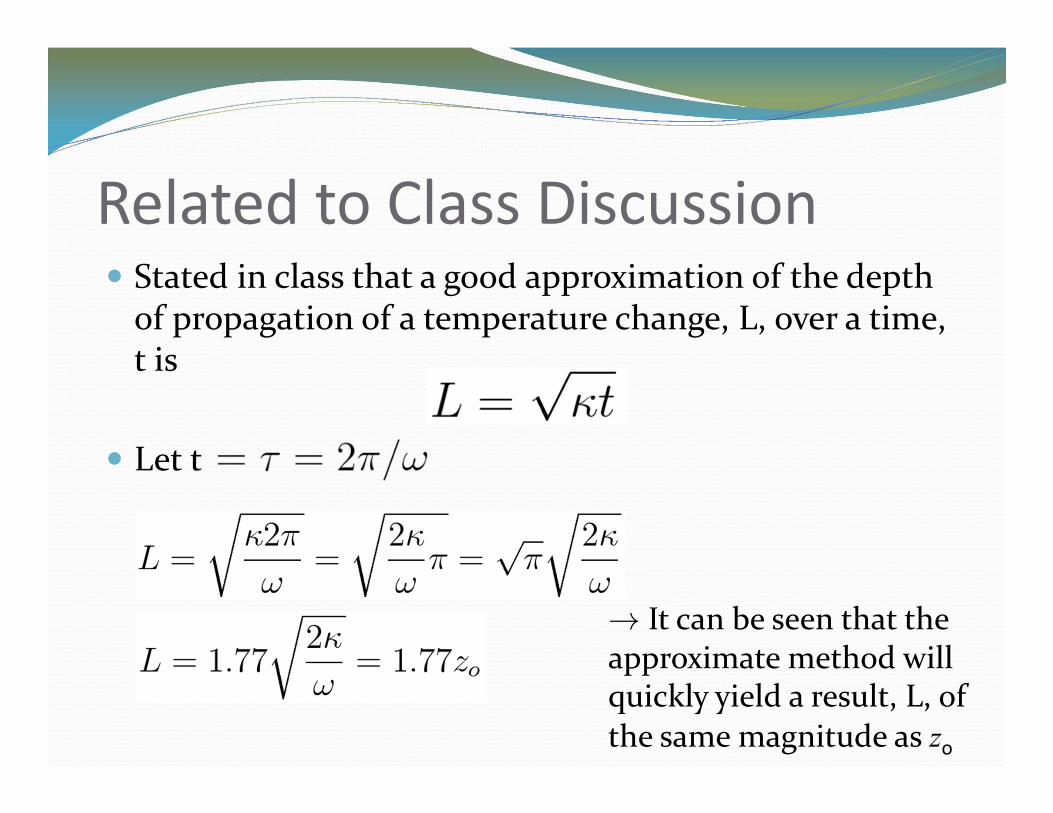
Related to Class Discussion Stated in class that a good approximation of the depth
of propagation of a temperature change, L, over a time, t is
Let t
→ It can be seen that the approximate method will quickly yield a result, L, of the same magnitude as zo

Attenuation Depth based on Soil Properties
Thermal diffusivity – soil property
Frequency – time-dependent
Ice Sandy Soil Clay Soil Peat Soil Rock
Κ (m2/s) 1.16 x 10⁻⁶ 0.24 x 10⁻⁶ 0.18 x 10⁻⁶ 0.10 x 10⁻⁶ 1.43 x 10⁻⁶
Diurnal Annual Glacial
ω (s-1) 7.27 x 10⁻⁵ 1.99 x 10⁻⁷ 4.98 x 10⁻¹²
http://apollo.lsc.vsc.edu/classes/met455/notes/section6/2.html

Attenuation Depth How deep is the attenuation depth or skin depth?
Represents depth where surface temperature can only affect by 37%
Ice Sandy Soil Clay Soil Peat Soil Rock
Diurnal 0.179 m 0.081 m 0.070 m 0.052 m 0.198 m
Annual 3.412 m 1.552 m 1.344 m 1.002 m 3.789 m
Glacial 682 m 310 m 268 m 200 m 757 m
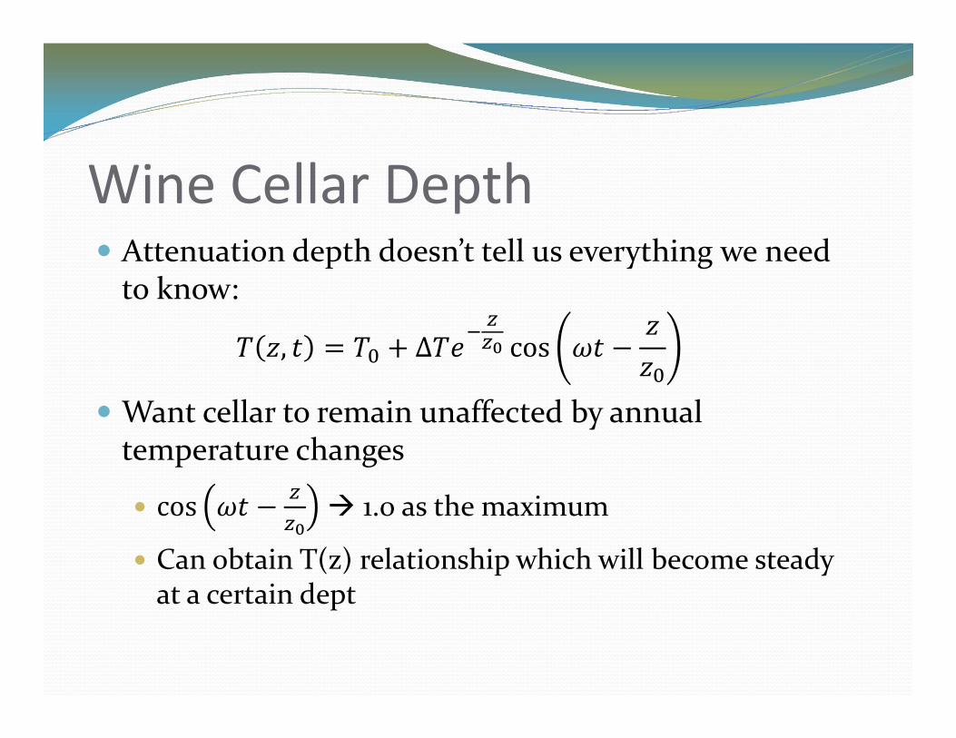
Wine Cellar Depth Attenuation depth doesn’t tell us everything we need
to know: , ∆ cos Want cellar to remain unaffected by annual
temperature changes
cos 1.0 as the maximum
Can obtain T(z) relationship which will become steady at a certain dept
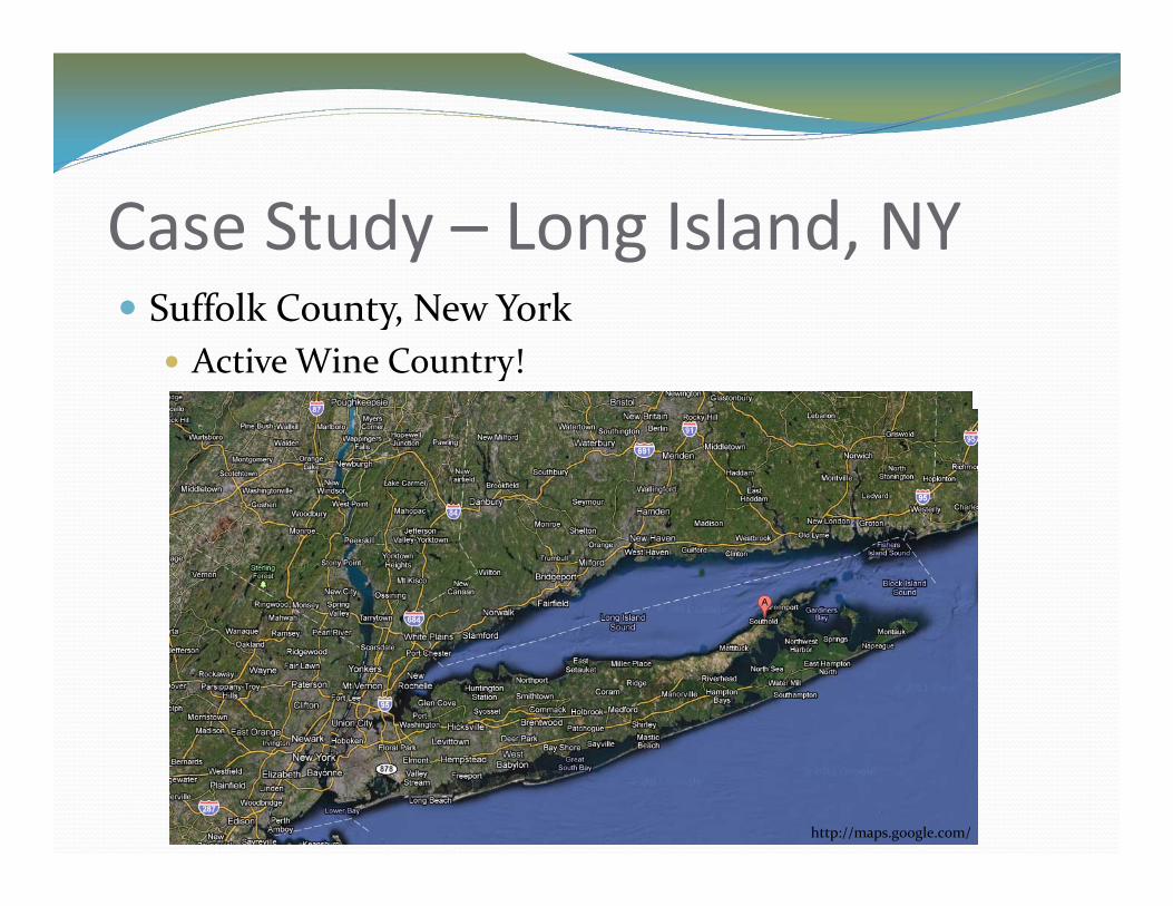
Case Study – Long Island, NY Suffolk County, New York
Active Wine Country!
http://maps.google.com/

Case Study – Long Island, NY Soil Type: well-drained, medium-moderately coarse
textured soils Sandy Soil: κ = 0.24 x 10⁻⁶
z0 = 1.552 m
New York Online Soil Survey. Retrieved from: http://soils.usda.gov/survey/online_surveys/new_york/
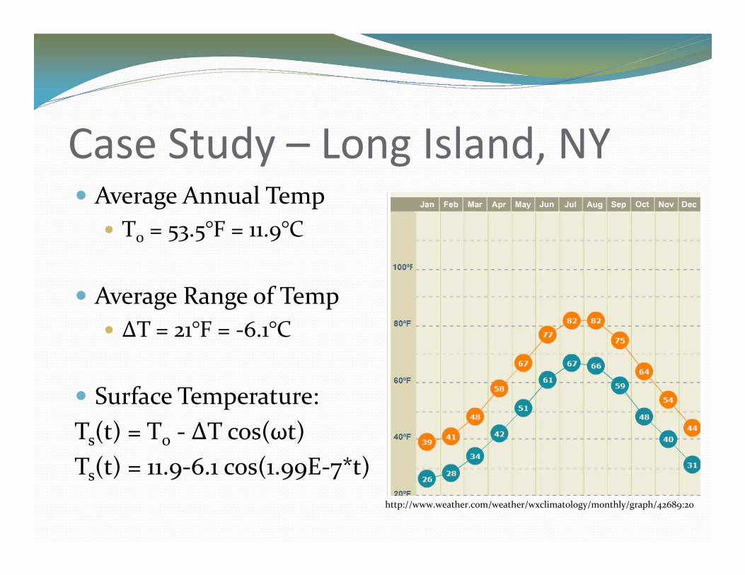
Case Study – Long Island, NY Average Annual Temp
T0 = 53.5°F = 11.9°C
Average Range of Temp ΔT = 21°F = -6.1°C
Surface Temperature:Ts(t) = T0 - ΔT cos(ωt)Ts(t) = 11.9-6.1 cos(1.99E-7*t)
http://www.weather.com/weather/wxclimatology/monthly/graph/42689:20

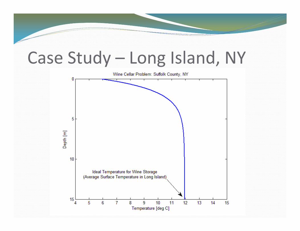
Case Study – Long Island, NY Recall: , ∆ cos Determined: temperature and attenuation
parameters Maximum effects require cosine term to 1 Now have:
maximum temperature effects along depth
Case Study – Long Island, NY
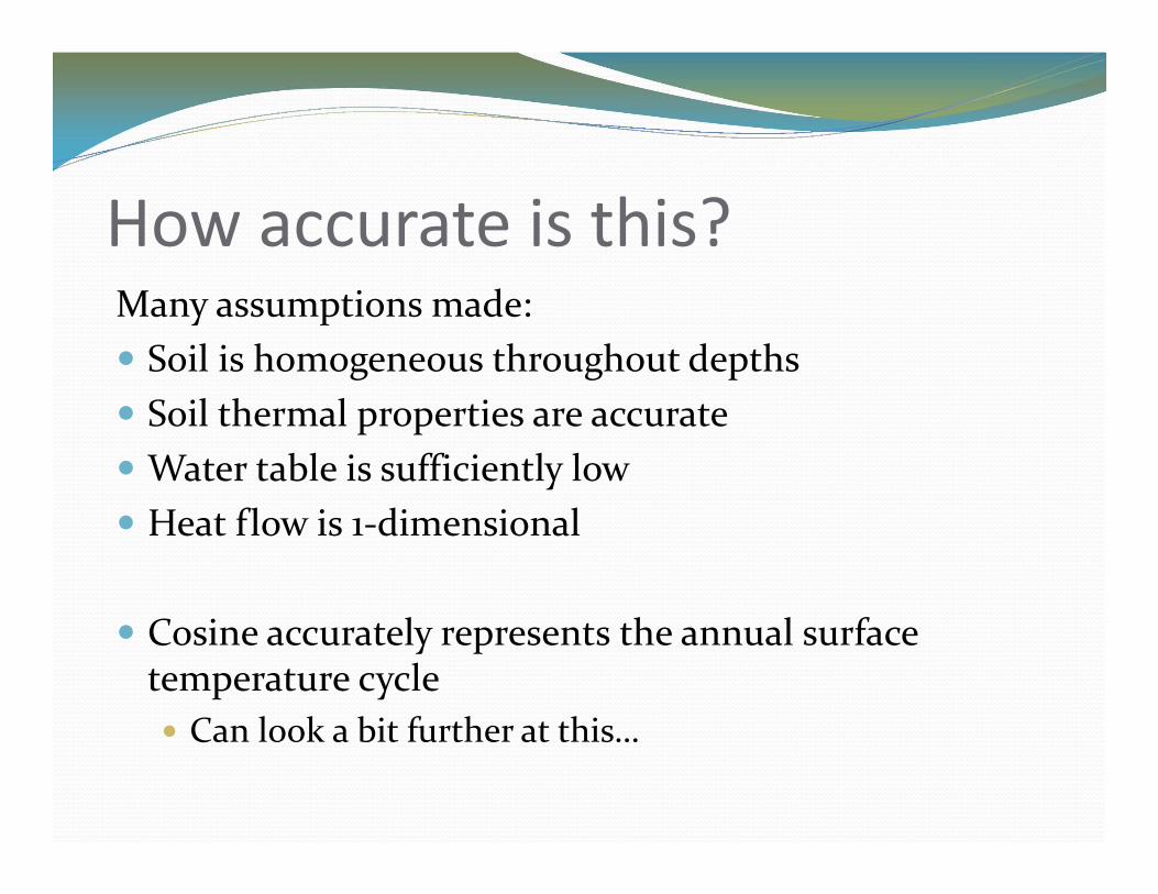
How accurate is this?Many assumptions made: Soil is homogeneous throughout depths Soil thermal properties are accurate Water table is sufficiently low Heat flow is 1-dimensional
Cosine accurately represents the annual surface temperature cycle Can look a bit further at this…

Borehole Comparison To take a look at the cosine representation
Measured borehole-thermistor data Thanks to the National Snow and Ice Data Center! Ilulissat, Greenland
Model forcing function as a cosine Compare!
Remember: Our model is only ever as good as our material (soil) properties! Soil type: Arctic brown soil Assume a diffusivity slightly greater than sandy soil
κ = 0.28

Borehole Comparison NSIC provided surface temperature data Fit a cosine function!
0 2 4 6 8 10 12 14-30
-20
-10
0
10
20
Time [yr]
Tem
pera
ture
[deg
C]
Surface Temperature Signal Determination
Measured Surface TemperatureTs = -3.5-11cos(2π t)
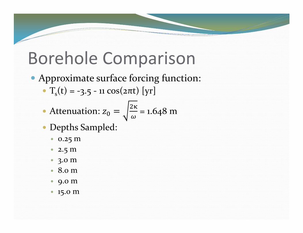
Borehole Comparison Approximate surface forcing function:
Ts(t) = -3.5 - 11 cos(2πt) [yr]
Attenuation: = 1.648 m
Depths Sampled: 0.25 m 2.5 m 3.0 m 8.0 m 9.0 m 15.0 m

Borehole Comparison
0 0.5 1 1.5 2 2.5 3 3.5 4 4.5
x 108
-14
-12
-10
-8
-6
-4
-2
0
2
4
6Modeled Temperature at Depth
Time [s]
Tem
pera
ture
[deg
C]
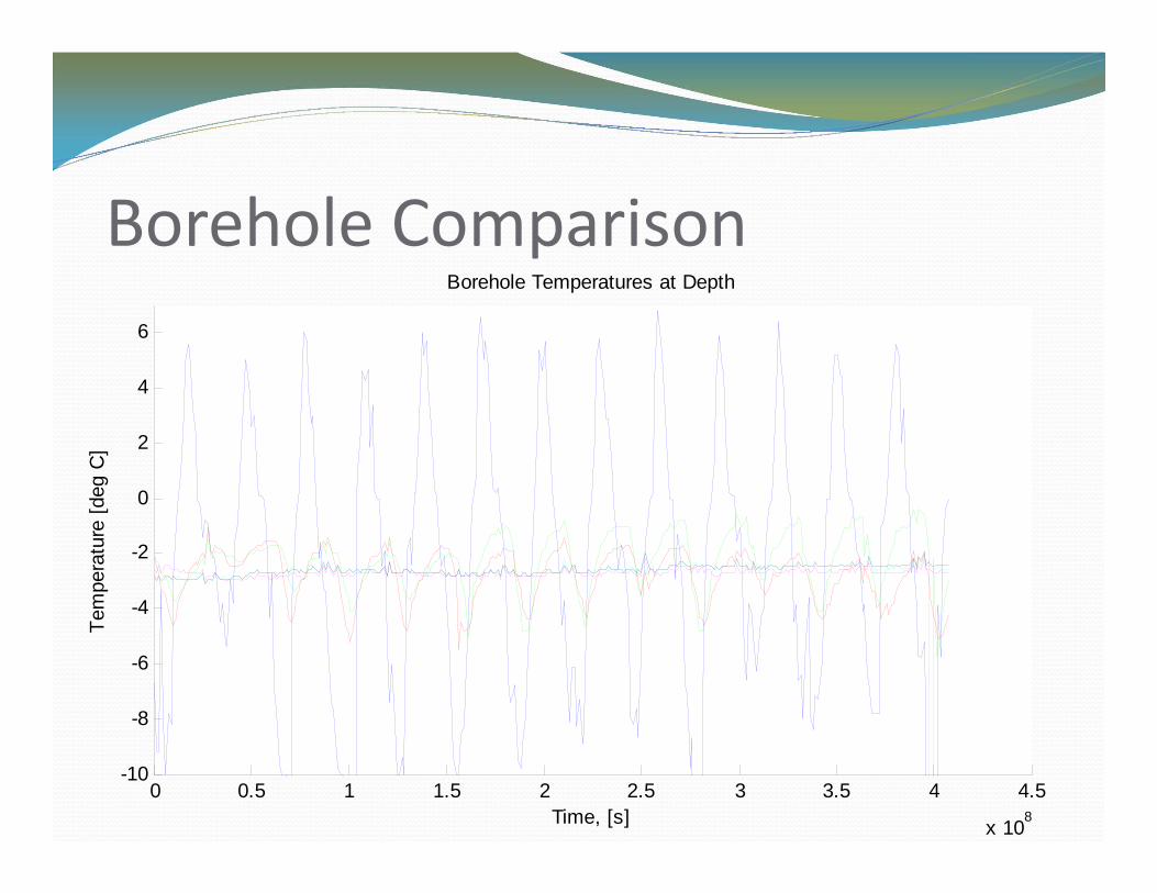
Borehole Comparison
0 0.5 1 1.5 2 2.5 3 3.5 4 4.5
x 108
-10
-8
-6
-4
-2
0
2
4
6
Time, [s]
Tem
pera
ture
[deg
C]
Borehole Temperatures at Depth

Borehole Comparison
0 0.5 1 1.5 2 2.5 3 3.5 4 4.5
x 108
-15
-10
-5
0
5
time
tem
p
Depth = 0.25m
MeasuredModeled
0 0.5 1 1.5 2 2.5 3 3.5 4 4.5
x 108
-15
-10
-5
0
5
time
tem
p
Depth = 3.0m
MeasuredModeled
0 0.5 1 1.5 2 2.5 3 3.5 4 4.5
x 108
-15
-10
-5
0
5
time
tem
p
Depth = 15.0m
MeasuredModeled
Conclusions Wine cellars ~ 8-10m beneath ground in Long Island Temperature at depth can be predicted
Cosine – a decent approximation to the annual temperature fluctuations
Soil properties are important! Even if model at surface is perfect, knowledge of soil at depths
is critical.
References Maps.google.com www.weather.com New York Online Soil Survey. Retrieved 25-Oct 2011 from:
http://soils.usda.gov/survey/online_surveys/new_york Basics of a Soil Layer Model. Retrieved 25-Oct 2011 from:
http://apollo.lsc.vsc.edu/classes/met455/notes/section6/2.html National Snow and Ice Data Center. Shallow Borehole Temperatures, Ilullisat, Greenland.
Retrieved 25-Oct 2011 from: http://nsidc.org/data/ggd631.html Turcotte, D. (2002). Geodynamics. Cambridge New York: Cambridge University Press. Pgs
149-152. Taler, J. (2006). Solving direct and inverse heat conduction problems. Berlin New York:
Springer. Pgs 366-374. Soil Mechanics: Design Manual 7.1. Alexandria, VA: Dept. of the Navy, Naval Facilities
Engineering Command, 1982.

Temperature as a function of depth and time
Paul Evans & Christine WittichSIO234: Geodynamics, Prof. Sandwell
Fall 2011