temperature measurement of a dust particle in a rf … measurement of a dust particle in ......
TRANSCRIPT
Temperature measurement of a dust particle in a RF plasma GEC
reference cell
Jie Kong, Ke Qiao, Lorin S. Matthews and Truell W. Hyde
Center for Astrophysics, Space Physics, and Engineering Research (CASPER)
Baylor University, Waco, Texas 76798-7310, USA
Abstract
The thermal motion of a dust particle levitated in a plasma chamber is similar to that described
by Brownian motion in many ways. The primary differences between a dust particle in a plasma
system and a free Brownian particle is that in addition to the random collisions between the dust
particle and the neutral gas atoms, there are electric field fluctuations, dust charge fluctuations,
and correlated motions from the unwanted continuous signals originating within the plasma
system itself. This last contribution does not include random motion and is therefore separable
from the random motion in a ‘normal’ temperature measurement. In this paper, we discuss how
to separate random and coherent motion of a dust particle confined in a glass box in a Gaseous
Electronic Conference radio frequency reference cell employing experimentally determined dust
particle fluctuation data analyzed using the mean square displacement technique.
1. Introduction
The coupling parameter for a dusty plasma system is defined as the ratio of the interparticle
potential energy to the dust kinetic (thermal) energy [1 – 3]. A two dimensional dust system
exhibits a phase transition from a liquid to crystalline state as the coupling parameter increases
beyond a critical value, c , where c is approximately 170 [4 – 6]. To determine this
system coupling parameter experimentally, a proper measurement of the dust kinetic energy, i.e.,
the dust temperature, is very important. By definition, the temperature of a dust particle is taken
to be
2
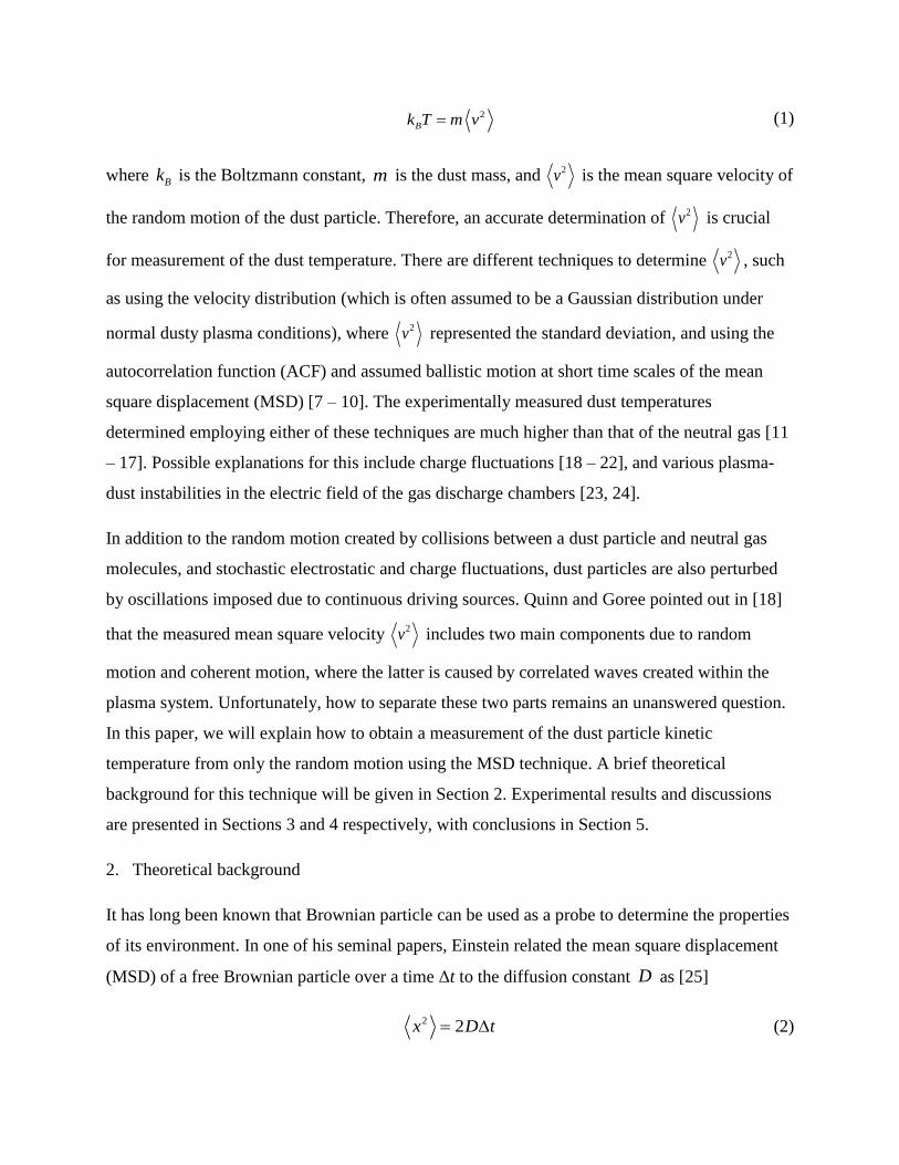
Bk T m v (1)
where Bk is the Boltzmann constant, m is the dust mass, and 2v is the mean square velocity of
the random motion of the dust particle. Therefore, an accurate determination of 2v is crucial
for measurement of the dust temperature. There are different techniques to determine 2v , such
as using the velocity distribution (which is often assumed to be a Gaussian distribution under
normal dusty plasma conditions), where 2v represented the standard deviation, and using the
autocorrelation function (ACF) and assumed ballistic motion at short time scales of the mean
square displacement (MSD) [7 – 10]. The experimentally measured dust temperatures
determined employing either of these techniques are much higher than that of the neutral gas [11
– 17]. Possible explanations for this include charge fluctuations [18 – 22], and various plasma-
dust instabilities in the electric field of the gas discharge chambers [23, 24].
In addition to the random motion created by collisions between a dust particle and neutral gas
molecules, and stochastic electrostatic and charge fluctuations, dust particles are also perturbed
by oscillations imposed due to continuous driving sources. Quinn and Goree pointed out in [18]
that the measured mean square velocity 2v includes two main components due to random
motion and coherent motion, where the latter is caused by correlated waves created within the
plasma system. Unfortunately, how to separate these two parts remains an unanswered question.
In this paper, we will explain how to obtain a measurement of the dust particle kinetic
temperature from only the random motion using the MSD technique. A brief theoretical
background for this technique will be given in Section 2. Experimental results and discussions
are presented in Sections 3 and 4 respectively, with conclusions in Section 5.
2. Theoretical background
It has long been known that Brownian particle can be used as a probe to determine the properties
of its environment. In one of his seminal papers, Einstein related the mean square displacement
(MSD) of a free Brownian particle over a time Δt to the diffusion constant D as [25]
2 2x D t (2)

where BD k T , with defined as the mobility. This relationship is only valid for time
intervals pt , where p is the momentum relaxation time. At very short time scales
(pt ) particle motion may be considered to be ballistic, as given by
2 2 2 2
Bx v t k T m t (3)
which characterizes the short time scale MSD for a Brownian particle.
Eqs 2 and 3 are derived assuming non-bounded particles, i.e., the Langevin equation for
describing the particle motion is free of any confinement force [26, 27]
mv m v R t (4)
where R t is the fluctuating force and 1 p is the damping coefficient [28].
For dust particles confined in a harmonic potential well, Eq 4 is modified to read as [29]
mx m x kx R t (5)
where 2
0k m and 0 is the particle resonance frequency. The MSD solution of Eq 5 is [10, 30]
(also see the Appendix A1 – A8),
2
0ˆ ˆ1 exp cos sin
ˆ2 2
tx A t t
(6)
where 0 2
0
2 Bk TA
m and
2
2
0ˆ
2
.
Eq 6 clearly shows that as t increases to 1t [31, 32],
2
0 210
2 B
t
k Tx A
m (7)

As can be seen, instead of being linearly proportional to t as in Eq 1, 2x is now a constant
which is related to both the kinetic temperature and the resonance frequency of the particle and is
independent of t . Experimentally the constant 0A is very easy to extract as will be shown in
the following section.
However, Eq 5 is based on an ideal system employing a harmonic confinement. For a dusty
plasma system with unwanted continuous oscillations, Eq 5 must be modified as,
cosi i
Correlated
mx m x kx R t a t (8)
where ia and i are the amplitude and frequency of individual oscillations within the system.
These unwanted oscillations may be mechanical or electronic. The corresponding solution for Eq
8 is (see A10 and A11 in the Appendix),
2
0ˆ ˆ1 exp cos sin cos
ˆ2 2i i i
Correlated
tx A t t C t
(9)
Eq 9 indicates that when 0 2
0
2 Bi
k TC A
m , and 1t , the mean square displacement
approaches an equilibrium value 0A with small modulations about this value of frequency i .
This means that these oscillations will not affect the constant 0A , which is related to the dust
temperature. The implication of this is that the experimentally determined average MSD at
1t is not affected by this continuous oscillation. Therefore, by measuring the constant 0A
the stochastic fluctuation can be separated from the correlated oscillations.
The kinetic energy supplied by the continuous oscillations to the dust particle is
2 21
2Corr i i
Corr
E m (10)
where i is the ith oscillation amplitude. Because this kinetic energy is proportional to the square
of the oscillation frequency, a greater contribution comes from higher frequency oscillations
when the amplitudes of all oscillations are similar.

The following sections describe a recent experiment which uses the natural random motion of a
single dust particle confined within a glass box placed on the lower powered electrode in a
Gaseous Electronic Conference (GEC) rf reference cell to verify Eqs 8 and 9. This is
accomplished by measuring the particle’s mean square displacement and then using this data to
derive both the oscillation frequency (i.e., the confinement force constant) and the temperature of
the dust particle.
3. Experiment and results
The experiments described here were conducted in one of CASPER’s GEC rf reference cells
[33]. Melamine formaldehyde (MF) dust particles having a diameter of 8.89 µm were introduced
into a glass box of dimension 10.5 mm × 10.5 mm × 12.5 mm (width × length × height) placed
on the lower powered electrode using a dust shaker mounted above the upper ring electrode. The
number of dust particles confined within the box was controlled by adjusting the system’s rf
power. A single confined dust particle was used for this experiment. For all experiments, a side
mounted high speed camera recorded 60 seconds of dust particle motion at 500 frames per
second (fps) (illuminated using a 50 mW solid state laser at 660 nm), neutral gas pressure was
held at 13.3 Pa and rf power was 2.25 W. An important aspect of the experimental setup is that
the DC bias of the lower electrode can be modulated using a function generator. This allows a
signal, consisting of a single frequency or random noise, to be sent to the lower electrode in
order to generate either correlated or random dust particle motion. For a single frequency input,
the frequency selected should be far from the dust particle’s intrinsic frequency, 0 , in order to
avoid resonance and reduce the mode coupling effects. In this experiment, a single frequency
input of 110 Hz was chosen. Adjusting the driving voltage allows the amplitude of the single
frequency or random noise to be controlled. Therefore, the values of 110i HzC C , and 0A in Eq 9
can be varied independently, i.e., 0A and 110HzC are now independent functions of the driving
voltage driveV . The original raw data (i.e., photos) are processed using “ImageJ” developed at
the National Institutes of Health [34]. Fig 1 shows representative raw data of dust particle
position fluctuations. The random noise driving amplitude was 2000 mV to show the difference
between the amplitude of induced vertical and horizontal oscillations.


Fig 1. Experimental data for a single dust particle’s position fluctuations. (a) Raw photo with
detected particle trajectory superimposed in green. (b) Horizontal and (c) vertical fluctuations as
a function of time derived from (a).
The particle’s mean square displacement (MSD) can be calculated from the experimental data
shown in Fig 1, and the dust particle’s corresponding temperature T, resonance frequency 0
and damping coefficient then derived using the theoretical fit provided by Eq 6. An example
MSD (under the conditions of no applied DC bias perturbation) is shown in Fig 2.

Fig 2. (a) Overview of a representative experimental MSD data set. (b) Expanded view of (a) for
1.0t s. Solid lines are experimental values and the dashed lines are the theoretical fit
calculated using Eq 6.
As can be seen in Fig 2, the MSDs are flat for a region 0.5 40t s. This constant value is 0A ,
which can be obtained by averaging over at least 42 10 data points under the experimental
setup of camera rate at 500 fps for 60 sec.
Fig 3 shows Fast Fourier Transformation (FFT) spectra for dust particle positions having
different values of driveV for both 110 Hz single frequency and random noise DC bias
modulations. The single frequency driving peak-to-peak voltage is measured before a 20 dB
attenuator.

Fig 3. FFT spectra of particle motion produced by modulation of the DC bias of the lower
electrode using a single frequency (a) – (c) and random noise (d) – (f). The amplitude of the
modulation is controlled by the driving voltage, as indicated in each panel. Only results for the
vertical direction are shown as there are no significant changes to the spectra for motion in the
horizontal direction in either case.
As can be seen in Fig 3, there is only minimal increase within the low frequency band (< 10 Hz,
where the dust intrinsic frequency, 0 , is located) as the single frequency driving voltage
increases (notice the difference in vertical scaling for each panel), while increasing the random
noise driving voltage has a strong effect on the low frequency band.
The effect of the modulation of the DC bias on the MSDs in the horizontal and vertical motion is
illustrated in Figure 4. The modulation of the DC bias using a single 110 Hz frequency had very
little effect on either the horizontal (4a) or vertical (4b) motion, and was only weakly dependent
on the magnitude of the driving amplitude. However, modulation of the DC bias employing
random noise increased the MSD in the vertical direction, with the magnitude of this increase
proportional to the driving amplitude (4d). There was no correlated effect on the MSD in the
horizontal direction (4c).

Fig 4. MSD for a 110 Hz single wavelength driving voltage at 200 mV and 1500 mV in the (a)
horizontal and (b) vertical directions, respectively. MSD for a random noise driving voltage at 0
mV and 1600 mV in (c) horizontal and (d) vertical directions, respectively.
As can be seen in Fig 4, horizontal (a) and vertical (b) equilibrium MSDs are only minimally
affected by changing the amplitude of a single-frequency modulation. On the other hand,
changing the amplitude of the random noise modulation causes the vertical equilibrium position
to shift significantly (d), while leaving the horizontal equilibrium MSD relatively unchanged (c).
Examining the MSD at short time scales reveals the small amplitude oscillations imposed in the
vertical direction by the 2000 mV, 110 Hz DC bias modulation (Fig 5), while the MSD in the
horizontal direction remains unaffected by the single frequency modulation.

Fig 5. (a) Comparison of the horizontal and vertical MSD for a 110 Hz single wavelength
modulation of the DC bias provided to the lower electrode. (b) Expanded view showing short
time scales.
As can be seen in Fig 5, the constant 0A can still be obtained by averaging the MSD over
0.5t s. However, the short time scale MSD is strongly affected by the 110 Hz oscillation in
the vertical direction.
4. Discussion
To verify Eq 9 experimentally, we must first prove that a random driving force is related to the
equilibrium value of the MSD. Since 0 2
0
2 Bk TA
m , and thus is directly related to the dust kinetic
temperature, a positive correlation between 0A and the amplitude of the random driving force
would imply that the random driving force also contributes to the dust kinetic temperature.

The dust particle temperature is derived using Eq 6. For this case, the drag will be assumed to be
to be given by the Epstein drag [28] in order to simplify the fitting process, with the drag
coefficient given by
8
d d th
p
r v
(11)
where the coefficient for diffuse reflection is 1.44 for MF dust particles in argon gas [35], dr
and d are the dust particle radius and density respectively, thv is the thermal velocity of the
neutral gas, and p is the pressure.
The equilibrium value 0A and the resonance frequency 0 can now be determined using Eq 6 to
fit the experimentally derived MSDs shown in Figures 2 and 5. The resonance frequencies found
in this manner are 0 0 2 7.0horiz horizf Hz, 0 6.6vertf Hz (for the non-driven oscillations
shown in Fig 2), and 0 0 2 7.8horiz horizf Hz, 0 0 2 6.5vert horizf Hz (for the single
frequency driven oscillations shown in Fig 5). The dust temperatures derived as a function of the
driving amplitude are shown in Fig 6 for both the random and single frequency driving signals.

Fig 6. The calculated dust temperature as a function of the driving amplitude for both a single
frequency and random driving signal in the (a) horizontal, and (b) vertical direction. Connecting
lines serve to guild the eye.
It can be seen that the dust temperature in the vertical direction increases as the driving
amplitude of the noise increases, while remaining almost constant in the horizontal direction.
This is due to the fact that DC modulation of the lower powered electrode creates a variation in
the confining electric field primarily in the vertical direction. In the vertical direction, the
supporting electric field force is balanced by the gravitational force acting on the dust particle,
which is constant. Therefore, changes in the vertical electric field represent an asymmetric
driving force which changes the instantaneous vertical equilibrium position of the particle, which
is added to the natural fluctuation about the equilibrium position. Changing the DC bias of the
lower electrode contributes a much smaller variation to the horizontal confining fields, with the
change being symmetric to each side. Thus the horizontal equilibrium position is not changed.
Secondly, it must be proved that a driving force consisting of a continuous single frequency
wave of constant amplitude, represented by i and iC in Eq 9, does not contribute to the dust

temperature. In this case, the kinetic temperature of the dust particle should not change as the
input amplitude of the continuous wave increases (as long as 0iC A ), since the continuous
wave should only induce small oscillations around the equilibrium value 0A . As shown in Fig 5,
a single frequency driving force imposes a modulation on the MSD in the vertical direction with
the same frequency as the driving force. This modulation does not significantly change the
equilibrium value 0A , but it does make calculation of the ballistic motion over the short time
regime ( 1 0.028t s for this experiment) very difficult if not impossible. Therefore,
employing the ballistic motion assumption, Eq 3, to calculate the dust temperature can be easily
affected by any unwanted coherent motion from the plasma system. On the other hand, as
pointed out in the previous section, the constant 0A can be calculated by averaging over a large
percentage of the collected data. This is another big advantage over the ballistic motion method,
which only consists a few data points.
In addition to the MSD and the short time scale techniques, the dust particle kinetic energy can
be obtained using the velocity probability distribution function (PDF). Representative velocity
PDFs from this experiment are shown in Fig 7. As shown, Gaussian distributions fit the
experimental data well in both the horizontal and vertical directions.

Fig 7. Representative velocity probability distribution functions (normalized) for driven noise
modulation with a driving amplitude of 100 mV. Symbols represent experimental values while
solid lines provide a theoretical Gaussian distribution fit.
The temperatures calculated from the Gaussian fit, where the standard deviation gives a measure
of 2
Gaussv which is related to the temperature by Eq 1, is shown in Fig 8 as a function of the
driving amplitude. This is compared to the temperatures calculated by the MSD technique.

Fig 8. Comparison of dust temperature derived using MSD technique (circles) and velocity
distribution function technique (crosses). Oscillations are driven using random noise.
The values for the temperature at a driving amplitude of 0 mV in Fig 8a are 0.052 eV and 0.35
eV as derived from the MSD and PDF of velocities respectively, which correspond to
approximately 600 K and 4000 K. Extrapolating the data to larger driving amplitudes as shown
(see the circled area around 5700 mV in Fig 8), the two extrapolated temperatures converge at a
certain point. This can be explained by assuming
Gauss real correlatedT T T (12)
where real MSDT T and correlatedT represents all the correlated oscillation contributions. Noting that
increasing the noise amplitude only increases MSDT , as the noise level increases to a point where
correlatedT can be ignored, eventually Gauss MSDT T .
As mentioned earlier, the continuous driving sources add kinetic energy to the dust particle (Eq
10). If not separated from the stochastic fluctuations, these oscillations lead to in apparent

increase in the dust temperature. The energy contributed by each oscillation frequency is
represented by the amplitude of the FFT spectra. It can be seen in Figure 3 that the system
(without added single-frequency or noise driven sources) shows small peaks at 55 Hz and 110
Hz. The amplitude of these oscillations is about 1 10 of the low frequency band ( 10 Hz).
Assuming that the contribution due to each of these frequencies is 10h , where h is the
standard deviation of the displacement for the non-driven case (Fig 3a). The total contribution to
the temperature can be calculated using Eqs 10 and 1. The excess temperature associated with
the 55 Hz is 55 560T K, and the excess temperature associated with the driving frequency 110
Hz is 110 2230T K. Adding these to the temperature derived from 0A using the MSD method,
the total temperature is 3400totalT K, close to the temperature determined from the Gaussian fit
to the velocity distribution shown in Figure 8, 4000GaussT K.
5. Conclusion
In this paper, temperature measurement of a dust particle in a dusty plasma chamber is discussed
in detail. Based on a MSD analysis, the contribution to the temperature measurement from
random fluctuations of a dust particle confined in a glass box in a GEC rf reference cell is
separated from the motion of a continuous single frequency perturbation. Theoretical analysis
and experimental data show that the equilibrium MSD at 1t is a function of the
amplitude of the driving random noise, but independent of the amplitude of a continuous single
frequency perturbation. Thus, a temperature derived using this method will be lower than that
using the velocity PDF method, where both the random and correlated motions are included in
the particle velocities, and thus a measurement of temperature is based on the energy of both
random and correlated motions. A real system will have particle motion driven by both random
forces (Brownian motion, fluctuations of the particle charge, fluctuations in the electric field,
etc.) as well as motion which is correlated with driving forces at a single frequency. It is
important to note that the MSD technique yields a temperature which includes energy
contributions from all random effects. However, it is not yet known how to distinguish between
the contributions of each of these effects which together form what is commonly referred to as
the temperature of the dust particle.


References
1. E. Wigner, “Effects of the electron interaction on the energy levels of electrons”, Trans.
Faraday Soc. 34, 678, (1938).
2. H. Thomas, G. E. Morfill, V. Demmel, and J. Goree, “Plasma crystal: Coulomb
crystallization in a dusty plasma”, Phys. Rev. Lett., 73, 652 – 655, (1994).
3. S. Ichimaru, “Strongly coupled plasmas: high-density classical plasmas and degenerate
electron liquids”, Rev. Mod. Phys. 54, 1017, (1982).
4. R. T. Farouki and S. Hamaguchi, “Thermodynamics of strongly-coupled Yukawa
systems near the one-component-plasma limit. II. Molecular dynamics simulations”, J.
Chem. Phys., 101, 9885, (1995).
5. Frank Melandso, “Heating and phase transitions of dust-plasma crystals in a flowing
plasma”, Phys. Rev. E 55, 7495, (1997).
6. Niels Otani and A. Bhattacharjee, “Debye Shielding and Particle Correlations in Strongly
Coupled Dusty Plasmas”, Phys. Rev. Lett., 78, 1468, (1997).
7. Tongcang Li, Simon Kheifets, David Medellin, Mark G. Raizen, “Measurement of the
instantaneous velocity of a Brownian particle”, Science, 328, 1673 – 1675, (2010).
8. Simon Kheifets, Akarsh Simha, Kevin Melin, Tongcang Li, Mark G. Raizen,
“Observation of Brownian motion in liquids at short times: instantaneous velocity and
memory loss”, Science, 343, 1493 – 1496, (2014).
9. Peter N. Pusey, “Brownian motion goes ballistic”, Science, 332, 802 – 803, (2011).
10. Christian Schmidt and Alexander Piel, “Stochastic heating of a single Brownian particle
by charge fluctuations in a radio-frequency produced plasma sheath”, Phys. Rev. E 92,
043106, (2015).

11. Hubertus M. Thomas and Gregor E. Morfill, “Melting dynamics of a plasma crystal”,
Nature, 379, 806, (1996).
12. A. Melzer, A. Homann, and A. Piel, “Experimental investigation of the melting transition
of the plasma crystal”, Phys. Rev. E 53, 2757, (1996).
13. Jeremiah D. Williams and Edward Thomas, Jr., “Initial measurement of the kinetic dust
temperature of a weakly coupled dusty plasma”, Phys. Plasmas, 13, 063509, (2006).
14. R. A. Quinn and J. Goree, “Single-particle Langevin model of particle temperature in
dusty plasmas”, Phys. Rev. E 61, 3033-3041, (2000).
15. Amit K. Mukhopadhyay and J. Goree, “Two-Particle distribution and correlation
function for a 1D dusty plasma experiment”, Phys. Rev. Lett., 109, 165003, (2012).
16. Amit K. Mukhopadhyay and J. Goree, Phys. Rev. Lett., 111, 139902, (2013).
17. J. B. Pieper and J. Goree, “Dispersion of plasma dust acoustic waves in the strong-
coupling regime”, Phys. Rev. Lett., 77, 3137, (1996).
18. R. A. Quinn and J. Goree, “Experimental investigation of particle heating in a strongly
coupled dusty plasma”, Phys. Plasmas, 7, 3904-3911, (2000).
19. V. V. Zhakhovski, V. I. Molotkov, A. P. Nefedov, V. M. Torchinski, A. G. Khrapak, and
V. E. Fortov, “Anomalous heating of a system of dust particles in a gas-discharge
plasma”, JETP Lett., 66, 419 – 425, (1997).
20. O. S. Vaulina, S. V. Vladimirov, A. Yu. Repin, and J. Goree, “Effect of electrostatic
plasma oscillations on the kinetic energy of a charged macroparticle”, Phys. Plasmas, 13
012111, (2006).
21. O. S. Vaulina, S. A. Khrapak, A. P. Nefedov, and O. F. Petrov, “Charge-fluctuation-
induced heating of dust particles in a plasma”, Phys. Rev. E 60, 5959 – 5964, (1999).

22. G. E. Morfill and H. Thomas, “Plasma crystal”, J. Vac. Sci. Technol. A 14, 490, (1996).
23. O. S. Vaulina, Plasma Phys. Rep., “Transport properties of nonideal systems with
isotropic pair interactions between particles”, 30, 652-661, (2004).
24. O. S. Vaulina, A. A. Samarian, B. James, O. F. Petrov, and V. E. Fortov, “Analysis of
macroparticle charging in the near-electrode layer of a high-frequency capacitive
discharge”, J. Experimental and Theoretical Physics, 96, 1037 – 1044, (2003).
25. Albert Einstein, “Uber die von der molekularkinetischen Theorie der Warme geforderte
Bewegung von in ruhenden Flussigkeiten suspendierten Teilchen”, Ann. Phys. (Berlin)
322, 549–560 (1905).
26. Ryogo Kubo, “The fluctuation – dissipation theorem”, Rep. Prog. Phys., 29, 255 – 283,
(1966).
27. Ryogo Kubo, “Brownian motion and nonequilibrium statistical mechanics”, Science,
233, 330 – 334, (1986).
28. Paul S. Epstein, “On the resistance experienced by spheres in their motion through
gases”, Phys. Rev. 23, 710 – 733, (1924).
29. M. C. Wang and G. E. Uhlenbeck, “On the theory of the Brownian motion II”, Rev. Mod.
Phys., 323 – 342, (1945).
30. Tongcang Li and Mark G. Raizen, “Brownian motion at short time scales”, Ann. Phys.
(Berlin), 525, 281 – 295, (2013).
31. V. Nosenko and J. Goree, “Laser method of heating monolayer dusty plasmas”, Phys.
Plasmas, 13, 032106, (2006).
32. Jie Kong, Ke Qiao, Lorin Matthews, and Truell W. Hyde, “Interaction force in a vertical
dust chain inside a glass box”, Phys. Rev. E 90, 013107, (2014).

33. Truell W. Hyde, Jie Kong, and Lorin S. Matthews, “Helical structures in vertically
aligned dust particle chains in a complex plasma”, Phys. Rev. E 87, 053106 (2013).
34. Wayne Rasband, National Institutes of Health, USA (http://imagej.nih.gov/ij).
35. Hendrik Jung, Franko Greiner, Oguz Han Asnaz, Jan Carstensen, and Alexander Piel,
“Exploring the wake of a dust particle by a continuously approaching test grain”, Phys.
Plasmas, 22, 053702, (2015).
36. Gregory H. Wannier, Statistical Physics, John Wiley and Sons, New York, 1966.
37. Paul Langevin. Sur la th´eorie du mouvement brownien. C. Rendus Acad. Sci. Paris,
146:530–533, 1908. Translated version: Don S. Lemons and Anthony Gythiel, Am. J.
Phys., 65, 1079 – 1081, (1997).
38. Robert Zwanzig. “Nonequilibrium statistical mechanics”, Oxford University Press, 2001.
39. Gerald R. Kneller, “Anomalous diffusion in biomolecular systems from the perspective
of non-equilibrium statistical physics”, Act Phys. Pol. B46, 1167 – 1199, (2015).
40. Gerald R. Kneller, “Stochastic dynamics and relaxation in molecular systems – Brownian
dynamics and beyond”, http://dirac.cnrs-orleans.fr/~kneller/SOCRATES/lecture.pdf.

Appendix
For a particle confined by a harmonic potential well, the Langevin equation is [36 – 39],
2
0mv m v m x R t (A1)
where is the damping coefficient, 0 is the dust resonance frequency, R t is the random
force, and m is the dust particle mass. Divide both sides by m,
2
0v v x r t (A2)
where r t R t m . A2 can be rewritten as,
2
00
t
v v v d r t (A3)
Multiplication with 0v and averaging over time yields [40]
2
00
0t
vv vv vvc c c d (A4)
where 0vvc v t v
is the velocity autocorrelation function (VACF), and 0 0v r t .
Applying Laplace transform to A4, the VACF is solved as,
1 2
ˆ Bvv
k T sc s
m s s s s
(A5)
where ˆvvc s is the Laplace transform of VACF, 1,2
ˆ2
s i
,
2
2
0ˆ
2
. The inverse
Laplace transform of A5 is the VACF
ˆ ˆexp cos sinˆ2 2
Bvv
k Tc t t t t
m
(A6)
To derive the MSD solution of A2, the following relationship between the VACF and MSD is
employed,
2
ˆ2ˆ Bsk T
W sm s
(A7)

where W s is the Laplace transform of MSD and ˆ s is the Laplace transform of normalized
VACF
2
0v t vt
v
. Therefore, the explicit form of MSD is,
2
2
0
2ˆ ˆ1 exp cos sin
ˆ2 2
Bk Tx t t t
m
(A8)
It is clear that as 1t ,
2
210
2 B
t
k Tx
m (A9)
For a system with continuous oscillation driving sources, A2 becomes,
2
0 cosi i
Correlated
v v x r t a t (A10)
where the sum runs over all continuous oscillation frequencies. The solution of A10 is, derived
using the same technique as the above on the homogeneous equation A4,
2
2
0
2ˆ ˆ1 exp cos sin cos
ˆ2 2
Bi i i
Corr
k Tx t t t C t
m
(A11)
When the driving oscillation frequency is greater than the resonance frequency, 0i , and its
amplitude is smaller 2
0
2 Bi
k TC
m , the oscillation driven MSD, A11, is just a small sinusoidal
oscillation imposed on the MSD solution of A8. Therefore, as 1t , the average value of A11
is the same as in A9.