tensor analysis - universität wien · tensor analysis author: harald höller ... the simple...

Tensor Analysis

Author: Harald Höller

last modified: 02.12.09

Licence: Creative Commons Lizenz by-nc-sa 3.0 at

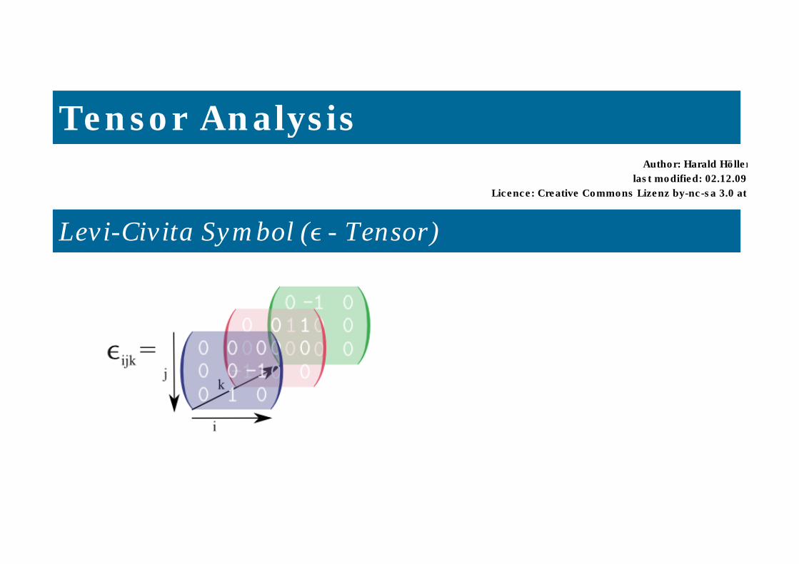
Levi-Civita Symbol (Ε - Tensor)

Ε = Ε = Ε = 1 123 231 312Ε = Ε = Ε = -1 132 213 321

Some useful relations between Ε -tensors and the Kronecker delta

Mathematica commands used in the following section

In[1]:= ? Sum

Sum@ f , 8i, imax<D evaluates the sum âi=1

imax

f.

Sum@ f , 8i, imin, imax<D starts with i = imin .

Sum@ f , 8i, imin, imax, di<D uses steps di.

Sum@expr, 8i, 8i1, i2, ¼<<D uses successive values i1, i2, ¼.

Sum@ f , 8i, imin, imax<, 8 j, jmin, jmax<, ¼D evaluates the multiple sum âi=imin

imax âj=jmin

jmax

¼ f.

In[2]:= ? Signature

Signature@listD gives the signature of the permutation needed to place the elements of list in canonical order.

In[3]:= ? KroneckerDelta

KroneckerDelta@n1, n2, ¼D gives the Kronecker delta ∆n1 n2 ¼, equal to 1 if all the ni are equal, and 0 otherwise.

2 Tensor_analysis_m6.nb

In[4]:= ? Table

Table@expr, 8imax<D generates a list of imax copies of expr.

Table@expr, 8i, imax<D generates a list of the values of expr when i runs from 1 to imax.

Table@expr, 8i, imin, imax<D starts with i = imin.

Table@expr, 8i, imin, imax, di<D uses steps di.

Table@expr, 8i, 8i1, i2, ¼<<D uses the successive values i1, i2, ¼.

Table@expr, 8i, imin, imax<, 8 j, jmin, jmax<, ¼D gives a nested list. The list associated with i is outermost.

In[5]:= ? MatrixForm

MatrixForm@listD prints with the elements of list arranged in a regular array.

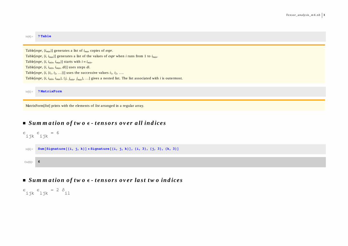
� Summation of two Ε - tensors over all indices

Ε Ε = 6 ijk ijk

In[6]:= Sum@Signature@8i, j, k<D *Signature@8i, j, k<D, 8i, 3<, 8j, 3<, 8k, 3<D

Out[6]= 6

� Summation of two Ε - tensors over last two indices

Ε Ε = 2 ∆ ijk ljk il

Tensor_analysis_m6.nb 3

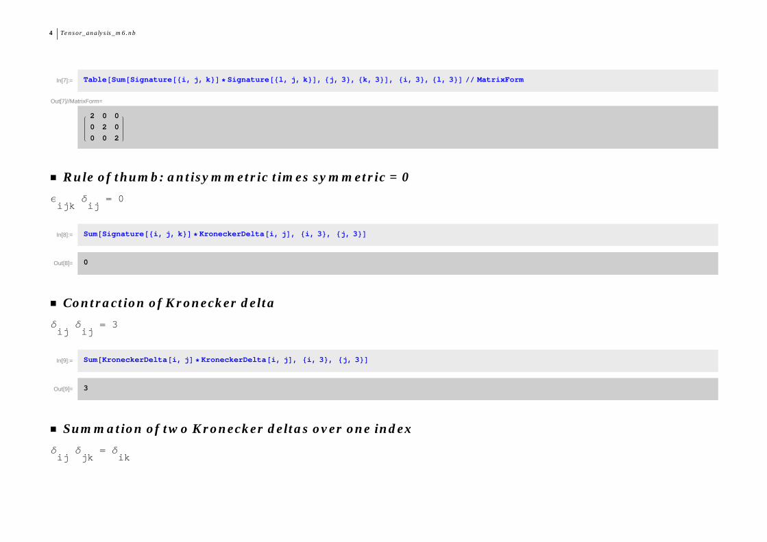
In[7]:= Table@Sum@Signature@8i, j, k<D *Signature@8l, j, k<D, 8j, 3<, 8k, 3<D, 8i, 3<, 8l, 3<D �� MatrixForm

Out[7]//MatrixForm=

2 0 0

0 2 0

0 0 2

� Rule of thumb: antisymmetric times symmetric = 0

Ε ∆ = 0 ijk ij

In[8]:= Sum@Signature@8i, j, k<D *KroneckerDelta@i, jD, 8i, 3<, 8j, 3<D

Out[8]= 0

� Contraction of Kronecker delta

∆ ∆ = 3 ij ij

In[9]:= Sum@KroneckerDelta@i, jD *KroneckerDelta@i, jD, 8i, 3<, 8j, 3<D

Out[9]= 3

� Summation of two Kronecker deltas over one index

∆ ∆ = ∆ ij jk ik


In[10]:= Table@Sum@KroneckerDelta@i, jD *KroneckerDelta@j, kD, 8j, 3<D, 8i, 3<, 8k, 3<D �� MatrixForm

Out[10]//MatrixForm=

1 0 0

0 1 0

0 0 1

Differential Operators in General Coordinates

Physics is full of differential operators and in many cases, the simple Euclidean vector space won't provide the coordinates of choice. Thus, often we

will have to transform into problem-oriented coordinate systems. With the package "VectorAnalysis", Mathematica supports a list of useful

tensorial operations, like gradient, divergence, rotation. In the following section we want to work out some applications to special coordinates

and once more compare the Mathematica-way with the "classical" approach.

In[11]:= Needs@"VectorAnalysis`"D

Nabla-operator in Cartesian coordinates

� Classical approach

The nabla operator is defined as the sum of derivations with respect to the coordinates times the corresponding base vector.

In Cartesian coordinates Iex, ey, ezMIn[12]:= ex := 81, 0, 0<

ey := 80, 1, 0<ez := 80, 0, 1<

this yields


this yields

In[15]:= Nabla @func_, x_, y_, z_D = D@func@x, y, zD, xD *ex + D@func@x, y, zD, yD *ey + D@func@x, y, zD, zD *ez

Out[15]= 9funcH1,0,0L@x, y, zD, funcH0,1,0L@x, y, zD, funcH0,0,1L@x, y, zD=

� Example: Scalar function R

We want to check the known relation

grad r =xÓ

r

and define as a scalar function the lenght of a vector x by r = x2

.

In[16]:= R@x_, y_, z_D := Sqrt@x^2 + y^2 + z^2D

In[17]:= Nabla@R, x, y, zD �� MatrixForm

Out[17]//MatrixForm=

x

x2+y2+z2

y

x2+y2+z2

z

x2+y2+z2

The gradient of a scalar is a tensor of rank 1 i.e. a vectorfield.


� Mathematica command Grad

At first we need to define the coordinate system. We need the following commands

In[18]:= ? SetCoordinates

SetCoordinates@coordsysD sets the default coordinate system to be coordsys with default variables.

SetCoordinates@coordsys@c1, c2, c3DD sets the default coordinate system to be coordsys with variables c1, c2, and c3.

In[19]:= ? Cartesian

Cartesian represents the Cartesian coordinate system with default variables Xx, Yy and Zz.

Cartesian@x, y, zD represents the Cartesian coordinate system with variables x, y, and z.

In[20]:= SetCoordinates@Cartesian@x, y, zDD

Out[20]= Cartesian@x, y, zD

The Grad command simply confirms the upper result.

In[21]:= ? Grad

Grad@ f D gives the gradient, Ñ f , of the scalar function f in the default coordinate system.

Grad@ f , coordsysD gives the gradient of f in the coordinate system coordsys.


In[22]:= Grad@Sqrt@x^2 + y^2 + z^2DD

Out[22]= :x

x2 + y2 + z2,

y

x2 + y2 + z2,

z

x2 + y2 + z2>

� Example: Vector field

In[23]:= P@x_, y_, z_D := :x

x2 + y2 + z2,

y

x2 + y2 + z2,

z

x2 + y2 + z2>

In[24]:= Nabla@P, x, y, zD �� FullSimplify

Out[24]= ::y2 + z2

Ix2 + y2 + z2M3�2, -

x y

Ix2 + y2 + z2M3�2, -

x z

Ix2 + y2 + z2M3�2>,

:-

x y

Ix2 + y2 + z2M3�2,

x2 + z2

Ix2 + y2 + z2M3�2, -

y z

Ix2 + y2 + z2M3�2>, :-

x z

Ix2 + y2 + z2M3�2, -

y z

Ix2 + y2 + z2M3�2,

x2 + y2

Ix2 + y2 + z2M3�2>>

The nabla operator applied on a tensor of rank 1 produces a tensor of rank 2. The divergence of our vector field P is given by the trace of the gradient

on P. The divergence is of course a scalar again.

In[25]:= ? Tr

Tr@listD finds the trace of the matrix or tensor list.

Tr@list, f D finds a generalized trace, combining terms with f instead of Plus.

Tr@list, f , nD goes down to level n in list.


In[26]:= Tr@Nabla@P, x, y, zDD

Out[26]= -

x2

Ix2 + y2 + z2M3�2-

y2

Ix2 + y2 + z2M3�2-

z2

Ix2 + y2 + z2M3�2+

3

x2 + y2 + z2

In[27]:= FullSimplify@%D

Out[27]=2

x2 + y2 + z2

Again we confirm with the Mathematica command (Div).

In[28]:= ? Div

Div@ f D gives the divergence, Ñ × f , of the vector field f in the default coordinate system.

Div@ f , coordsysD gives the divergence of f in the coordinate system coordsys.

In[29]:= DivB:x

x2 + y2 + z2,

y

x2 + y2 + z2,

z

x2 + y2 + z2>F �� FullSimplify

Out[29]=2

x2 + y2 + z2


Nabla Operator in spherical coordinates

� The Mathematica-way

In[30]:= Clear@"Global`*"D

In[31]:= ? Spherical

Spherical represents the spherical coordinate system with default variables Rr, Ttheta and Pphi.

Spherical@r, Θ, ΦD represents the spherical coordinate system with variables r, Θ and Φ.

In[32]:= SetCoordinates@Spherical@r, Θ, ΦDD

Out[32]= Spherical@r, Θ, ΦD

In[33]:= Grad@rD

Out[33]= 81, 0, 0<

In[34]:= Div@81, 0, 0<D

Out[34]=2

r


� Alternatively

Define spherical coordinates by their transformation rules

In[35]:= x := r Sin@ΘD Cos@ΦDy := r Sin@ΘD Sin@ΦDz := r Cos@ΘD

and determine the Jacobian of the transformation

In[38]:= Tij = 88D@x, rD, D@x, ΘD, D@x, ΦD<, 8D@y, rD, D@y, ΘD, D@y, ΦD<, 8D@z, rD, D@z, ΘD, D@z, ΦD<<

Out[38]= 88Cos@ΦD Sin@ΘD, r Cos@ΘD Cos@ΦD, -r Sin@ΘD Sin@ΦD<, 8Sin@ΘD Sin@ΦD, r Cos@ΘD Sin@ΦD, r Cos@ΦD Sin@ΘD<, 8Cos@ΘD, -r Sin@ΘD, 0<<

and determine the base vectors.

In[39]:= er = Transpose@TijD@@1DDeΘ = Transpose@TijD@@2DDeΦ = Transpose@TijD@@3DD

Out[39]= 8Cos@ΦD Sin@ΘD, Sin@ΘD Sin@ΦD, Cos@ΘD<

Out[40]= 8r Cos@ΘD Cos@ΦD, r Cos@ΘD Sin@ΦD, -r Sin@ΘD<

Out[41]= 8-r Sin@ΘD Sin@ΦD, r Cos@ΦD Sin@ΘD, 0<


In[42]:= Nablaspher @func_, r_, Θ_, Φ_D = D@func@r, Θ, ΦD, rD *er + D@func@r, Θ, ΦD, ΘD *eΘ + D@func@r, Θ, ΦD, ΦD *eΦ

Out[42]= 9-r Sin@ΘD Sin@ΦD funcH0,0,1L@r, Θ, ΦD + r Cos@ΘD Cos@ΦD funcH0,1,0L@r, Θ, ΦD + Cos@ΦD Sin@ΘD funcH1,0,0L@r, Θ, ΦD,r Cos@ΦD Sin@ΘD funcH0,0,1L@r, Θ, ΦD + r Cos@ΘD Sin@ΦD funcH0,1,0L@r, Θ, ΦD + Sin@ΘD Sin@ΦD funcH1,0,0L@r, Θ, ΦD,-r Sin@ΘD funcH0,1,0L@r, Θ, ΦD + Cos@ΘD funcH1,0,0L@r, Θ, ΦD=

In[43]:= Assuming@r > 0, FullSimplify@Sqrt@x^2 + y^2 + z^2DDD

Out[43]= r

In[44]:= Rspher@r_, Θ_, Φ_D := r

In[45]:= Nablaspher@Rspher, r, Θ, ΦD �� FullSimplify

Out[45]= 8Cos@ΦD Sin@ΘD, Sin@ΘD Sin@ΦD, Cos@ΘD<

The same result looks quite different than the constant vector {1,0,0} from the Mathematica-way. However, the result is in perfect agreement, since

it is only a different way of expressing the unit vector in r-direction.

In[46]:= % � er

Out[46]= True


tensor analysis - universität wien · tensor analysis author: harald höller ... the simple...

Documents