tensor field visualization

Tensor Field Visualization

Direct Methods:

Pseudo-colors and Glyphs

Pseudo-Colors

• Any derived scalar properties of the tensor can be mapped to color plots

• Assume a tensor T is defined at each vertex

– Components (or entries) ��– Tensor magnitude

� � � 12��

– Trace, � � � ∑��. If T is the Jacobian of a flow field, this tells how much divergence it has.

Pseudo-Colors

Divergence and curl of a vector field

Pseudo-Colors

• Scalar properties of tensor (continued)

– Determinant

– Eigen-values

• � � λ • Can be used to compute the determinant for

diagonalizable tensor

• More importantly, it can be used to study the

anisotropy of the symmetric tensor, e.g.

diffusion tensor used in medical applications

Anisotropy direction

+ strength mapped

to saturation

Glyphs

• 1D shapes: the simplest is to map each eigen-

vector direction to a line segment with length

corresponding to the strength (i.e. eigen-value)

• 2D/3D shapes: better visualization of the local

property of tensor, such as anisotropy

The glyphs for visualizing the anisotropy of a symmetric tensor

Geometric-based Method

Hyperstreamlines

• Let T(x) be a (2nd order) symmetric tensor field– real eigenvalues, orthogonal eigenvectors

• Hyperstreamline: by integrating along one of the eigenvectors

• Important: Eigenvector fields are not vector fields!

– eigenvectors have no magnitude and no orientation (are bidirectional)

– the choice of the eigenvector can be made consistently as long as eigenvalues are all different

– Hyperstreamlines can intersect only at points where two or more eigenvalues are equal, so-called degenerate points.

Red – major

Green – minor

Compute One Hyperstreamline

• Choose integrator:– Euler

– Runge-Kutta

• Choose step size (can be adaptive)

• Provide seed point position and determine starting direction

• Advance the front

• Note that the angle ambiguity. This is because the computation of the eigenvector at each sample point (i.e. vertex of the mesh) is independent of each other. Therefore, inconsistent directions may be chosen at neighboring vertices. – Additional step to remove angle ambiguity. A dot product between the

current advancing direction and the eigenvector direction at current position is performed. A positive value indicates the consistent direction; otherwise, the inverse direction should be used!

Evenly-Spaced Placement

• Input: – dsep … start distance

– dtest … minimum distance

• Compute an initial hyperstreamline from a random seed point, put to queue

• Compute a set of candidate seeds that are dsep away from the initial hyperstreamline, put to queue

• current hyperstreamline = initial hyperstreamline

• WHILE not finished DO:– TRY: get new seed point which is dsep away from current hyperstreamline

– IF successful THEN

• compute new hyperstreamline until distance dtest is reached (or other…) AND put to queue

– ELSE IF no more hyperstreamline in queue THEN

• exit loop

– ELSE next hyperstreamline in queue becomes current hyperstreamline

– [Jobard and Lefer 1997; Alliez et al. 2003; Zhang et al. 2007]

Our methodThe method based on

Jobard and Lefer’s

Hyper-Streamline PlacementHyper-Streamline Placement

According to different applications, the termination conditions may be different

Hyperstreamlines

Widely used in diffusion tensor imaging tractography

Hyperstreamlines rendered as

tubes with elliptic cross section,

radii proportional to 2nd and 3rd

eigenvalue

[Shen and Pang 2004]

Hyperstreamlines

Hyperstreamlines can also be

used to convey some physical

behaviors in the tensor. For

instance, in flow analysis, the

hyperstreamlines computed

based on the eigen analysis of

the Jacobian of the flow field

can convey stretching and

rotational flow deformation

[Zhang et al. TVCG 2009]

Hyperstreamlines

Hybrid visualization: hyperstreamlines + glyphs

Good for some non-symmetric tensor visualization where the rotational

components can be encoded by the glyphs

[Prckovska et al. 2010]

Problem of Hyperstreamlines

• Ambiguity in (nearly) isotropic regions:

– Partial voluming effect, especially in low resolution images

(MR images)

– Noise in data

– Solution: tensorlines

[Weinstein, Kindlmann 1999]

Tensorline

Hyperstreamline

Arrows: major eigenvector

• Advection vector

• Stabilization of propagation by considering

• Input velocity vector

• Output velocity vector (after application of tensor operation)

• Vector along major eigenvector

• Weighting of three components depends on anisotropy at specific position:

• Linear anisotropy: only along major eigenvector

• Other cases: input or output vector

Texture-based Method

HyperLIC

The LIC pipeline

[Zheng and Pang]

Instead using a 1D kernel along the

streamline, HyperLIC uses a 2D kernel

�� is the input and �� is the outputλ� � , � � , � �, � , � � 1,2 are the nth

eigenvalues, eigenvectors and the weight

function at point X. ∆is the integration step.

HyperLIC

The LIC pipeline

[Zheng and Pang]



If we define

Decompose the computation

HyperLIC

The LIC pipeline

[Zheng and Pang]



Then

This is a two-pass process

��and ��are the output images of the un-

normalized LIC on λ and λ� � vector fields

with input images ��and ��, respectively.


HyperLIC

The LIC pipeline

[Zheng and Pang]



Then

This is a two-pass process

Theoretically, the order in which the eigenvector

fields are processed will affect the final image. In

practice, the differences are not noticeable


Some Results

A 2D slice from single point load stress tensors. It is taken from the middle of

the volume and viewed from the point load direction. It is mostly composed of

components from medium or minor eigenvectors. We see that the center of

this slice is quite isotropic. Around the center is a ring formed by lines, which

means tensors are highly anisotropic. It is the boundary where the minor

eigenvalues are zero.

Some Results

Flow past a cylinder with hemispherical cap. HyperLIC of two different

computational layers of the strain rate tensor. Arrows point to

locations of degenerate wedge points

A Simplified HyperLIC

• Compute two LIC images along the major

and minor eigen-vector fields,

respectively.

• These two computations are independent

of each other, and thus, can be

parallelized.

• Note, the angle ambiguity needs to be

properly handled as in the

hyperstreamline tracing.

• NOTE, this is only meaningful for

symmetric positive definite tensors

The image represents a xz-plane slice of a

two-force dataset. The left circle

corresponds to the pushing and the right to

the pulling force. The fluctuation of the

color is a result of the low resolution of the

simulation[Hotz et al. 2004]

Review IBFV

Extended IBFV

(a) (b)

(c) (d)

Consider a s.p.d tensor field T. Let D denote the

domain and �be the set of points in D where V is

discontinuous. While it is not always possible to

construct a vector field V from T such that � � �∅, we build two vector fields �� and �such that ⋂ � ��!� contains only the degenerate points of T,

and every regular point in the domain belongs to "\S ��!for some i.

Its major eigenvector field can be represented in

terms of two spatially varying scalar fields % and &,

which are the magnitude and direction, respectively.

'� � (% cos&sin & ρ / 0!

IBFV does not trace out streamlines. So it cannot

address the angle ambiguity explicitly!

[Zhang et al. TVCG07]

Extended IBFV

(a) (b)

(c) (d)

'� � (% cos&sin & ρ / 0!We define the following two vector fields from '�

�1 is obtained from '� by choosing directions so that the x-

component of �1 is nonnegative everywhere. Therefore � �1 � 2, 3 | cos & 2, 3 � 0




Extended IBFV

(a) (b)

(c) (d)

Let �1 and �5be the images produced using

IBFV with �1 and �5Let 61 � cos & and 65 � sin & � 1 7 cos &be the blending functions. Then, the final image� � 61 �1 8 65�5 produces the desired result.

The system first produces images according to two direction assignments: ((a), in the positive

x-direction) �1 and ((b), in the positive y-direction) �5 . The images are then blended according

to weight functions 61 (a color coding shown in (c)) and 65 � 1 7 61. (d) The resulting image

no longer contains the visual artifacts from �1 and �5 .




Some Results


Extension to N-Symmetric Field

Visualization [Palacios and Zhang TVCG 2011]

Glyph-based Methods

Glyphs for Tensors

• 2D/3D shapes: better visualization of the local property of

tensor, such as anisotropy

The glyphs for visualizing the anisotropy of a symmetric tensor

3D

2D

Glyphs for Tensors

Consider symmetric tensors at this moment. They have real

eigenvalues and orthogonal Eigenvectors. Therefore, they can be

intuitively represented as ellipsoids.

Three types of anisotropy:

• linear anisotropy

• planar anisotropy

• isotropy (spherical)

Anisotropy measure

9: � λ� 7 λ! λ� 8 λ 8 λ;!<9= � 2 λ 7 λ;! λ� 8 λ 8 λ;!<

9> � 3λ; λ� 8 λ 8 λ;!@λ� / λ / λ;

Image by G. Kindlmann

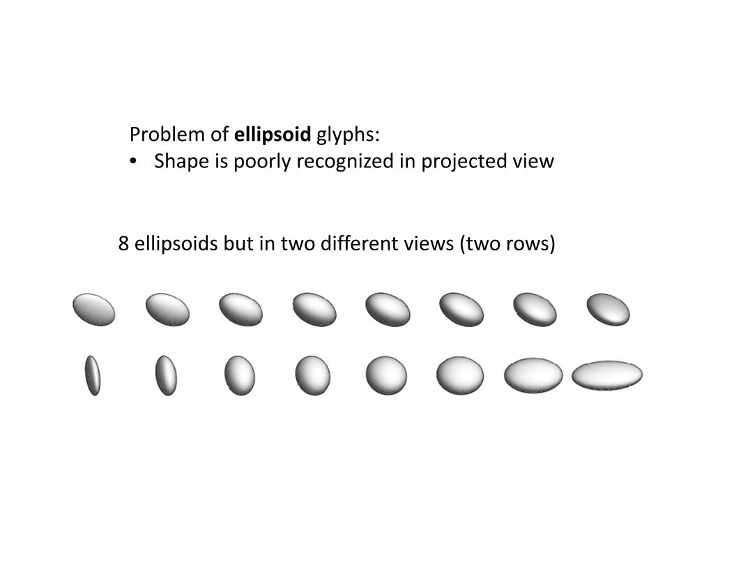
Problem of ellipsoid glyphs:

• Shape is poorly recognized in projected view

8 ellipsoids but in two different views (two rows)

Problem of cuboid glyphs

• Missing symmetry

Problem of cylinder glyphs

• Seam at 9: � 9=• Losing symmetric close to9> � 1

Combining advantages: superquadrics

Superquadrics with z as primary axis

AB &, ∅ � cosC&sinD∅sinC&sinD∅cosD∅0 E & E 2F, 0 E ∅ E 2F Superquadrics for some pairs G, H!Shaded: sub-range used for glyphs

Barr, 1981

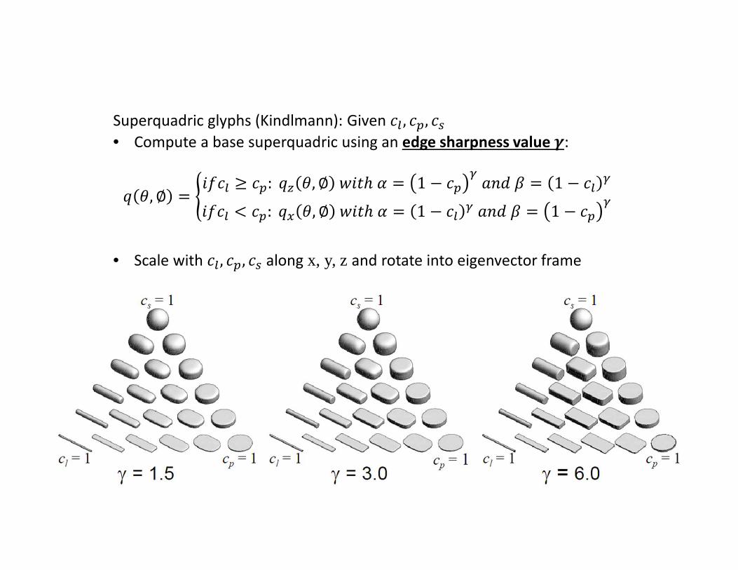
Superquadric glyphs (Kindlmann): Given 9: , 9=, 9>• Compute a base superquadric using an edge sharpness value I:

A &, ∅ � J�K9: / 9=: AB &, ∅ M�NG � 1 7 9= OP�QH � 1 7 9: O�K9: R 9=: A1 &, ∅ M�NG � 1 7 9: OP�QH � 1 7 9= O

• Scale with 9: , 9=, 9> along x, y, z and rotate into eigenvector frame

Comparison of shape perception (previous example)

• With ellipsoid glyphs

• With superquadrics glyphs

Comparison: Ellipsoids vs. superquadrics (Kindlmann)

Color mapSTU � 9:

| 1�|| 5�|| B�|

8 1 7 9:! 111This is half of the brain, looking at the posterior part of the

corpus callosum, which is the main bridge between the two

hemispheres. And with the superquadrics, you can see that

on the surface of the corpus callosum, the glyphs have

more of a planar component, but on the inside, they're

basically very linear.

[Schultz and Kindlmann, Vis10]

Superquadric Glyphs for Symmetric Second-Order Tensors

Extended to general second-order symmetric tensors that can be indefinite

Glyph Packing

[Kindlmann and Westin, Vis06]

Reduce holes, overlaps, and artifacts

• Basic pipeline

– Seeding based on some statistical property

– Force repelling *

• Each particle tries to push away its neighboring

particles

• This process should eventually converge to a stable

configuration.

– Rendering glyphs

Energy-based Particle Systems

Energy-based Particle Systems

Computation of the

Energy


G is the glyph scaling factor

Computation of the

Forces


G is the glyph scaling factor

Improvement- Parallel Computation

Original method considers all the particles in the domain

Improvement- Parallel Computation

[Kim et al. GPGPU5]

Multithreaded (cont)

� Given the current bin Bi

� Gather every particle in Biplus the immediate

surrounding bins

− This is a neighborhood

� For every particle piin the bin B

i

− For every particle pjin the neighborhood

� If distance from pito p

j< 1.0

− sum the velocity and energy

− Advect pi

[Kim et al. GPGPU5]

Multithreaded (cont.)

Current Bin

� Process each

particle in the

current bin

[Kim et al. GPGPU5]


Current Particle

� Process each

particle in the

current bin

[Kim et al. GPGPU5]


� sum Energy

and Force

[Kim et al. GPGPU5]


� Move current

particle

[Kim et al. GPGPU5]


� Process the

next particle in

the current

bin.

[Kim et al. GPGPU5]

Y Z

W X

Multithreaded (cont)

� While there are bins to be

processed

− For every particle p in the current

bin

� For every other particle in the

neighborhood

− calculate force and energy

� Move the particle in the direction F

[Kim et al. GPGPU5]

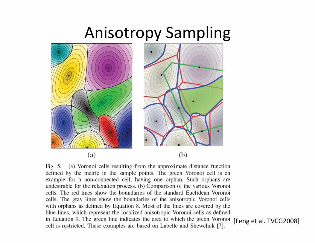
Anisotropy Sampling

[Feng et al. TVCG2008]


Anisotropy Sampling

Glyph Packing in Bounded Regions

[Chen et al. Vis11]

tensor field visualization

Documents