tensorflow 深度學習快速上手班--機器學習
TRANSCRIPT
TensorFlow深度學習快速上⼿手班������
⼀一、機器學習
By Mark Chang
⼤大綱 • 機器學習簡介 • Tensorflow簡介 • Tensorflow安裝 • 單層感知器實作

機器學習簡介
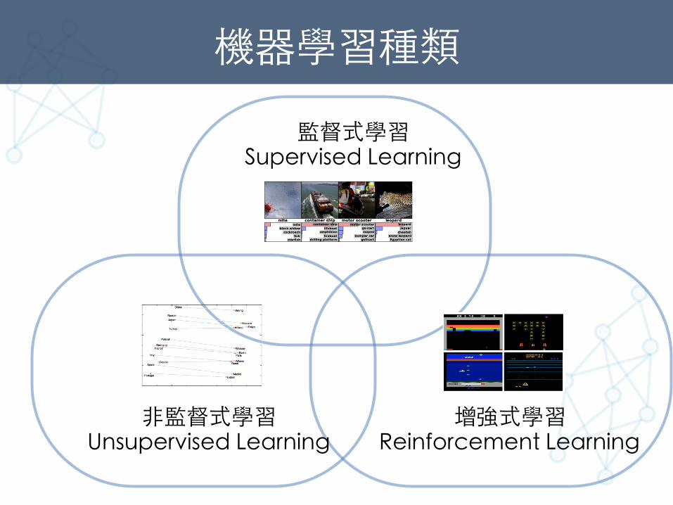
機器學習種類
監督式學習 Supervised Learning
⾮非監督式學習 Unsupervised Learning
增強式學習 Reinforcement Learning
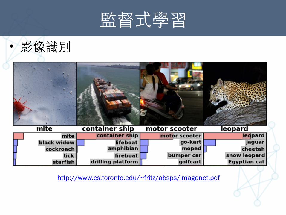
監督式學習 • 影像識別
http://www.cs.toronto.edu/~fritz/absps/imagenet.pdf
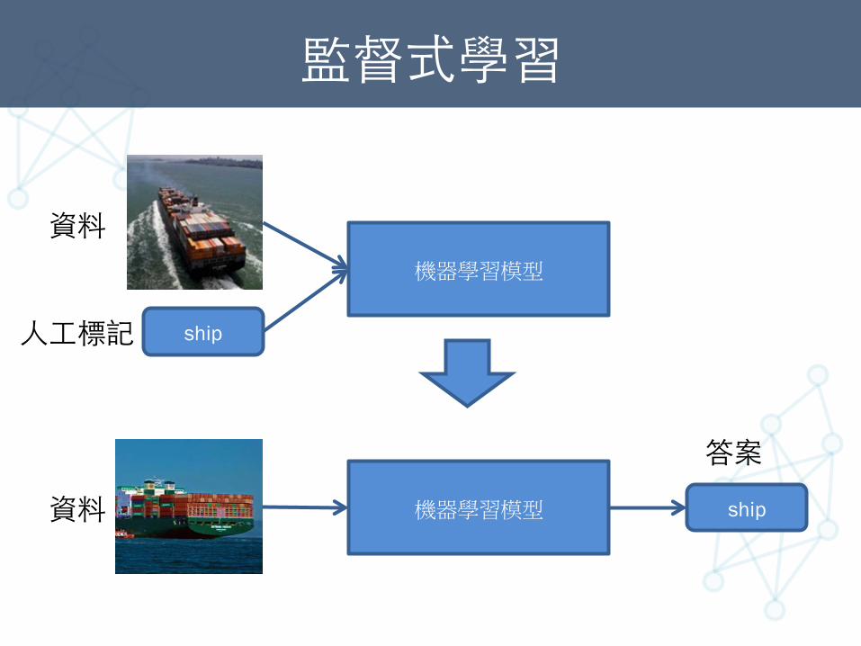
監督式學習
機器學習模型
機器學習模型 ship
ship
資料
⼈人⼯工標記
資料
答案
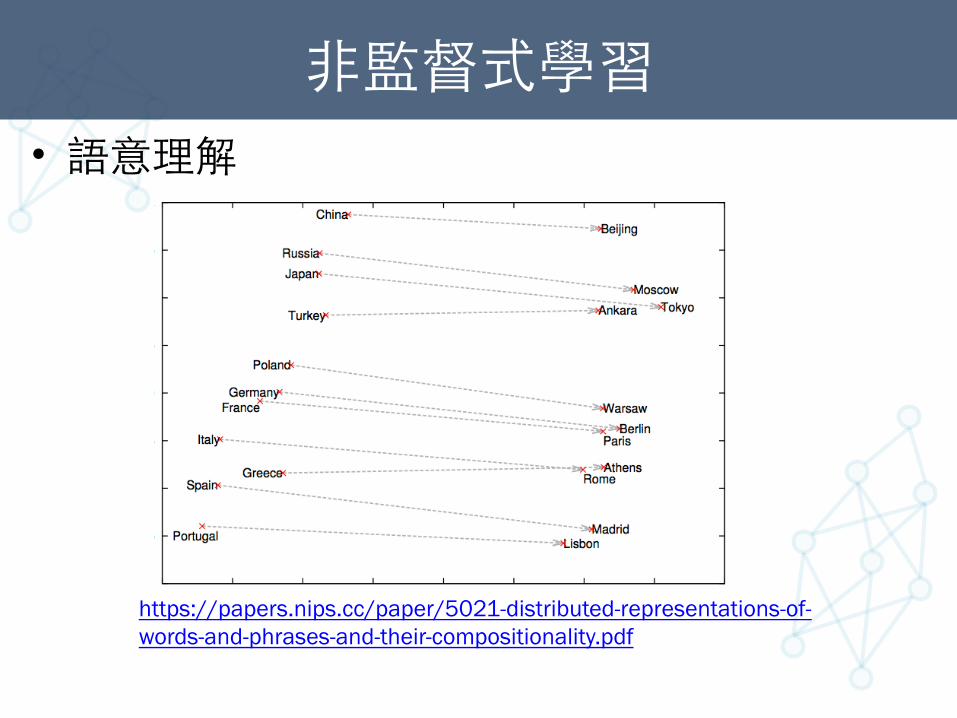
⾮非監督式學習 • 語意理解
https://papers.nips.cc/paper/5021-distributed-representations-of-words-and-phrases-and-their-compositionality.pdf
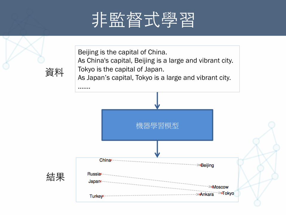
⾮非監督式學習
機器學習模型
Beijing is the capital of China. As China's capital, Beijing is a large and vibrant city. Tokyo is the capital of Japan. As Japan’s capital, Tokyo is a large and vibrant city. …….
資料
結果

增強式學習 • 打電動
http://arxiv.org/pdf/1312.5602v1.pdf
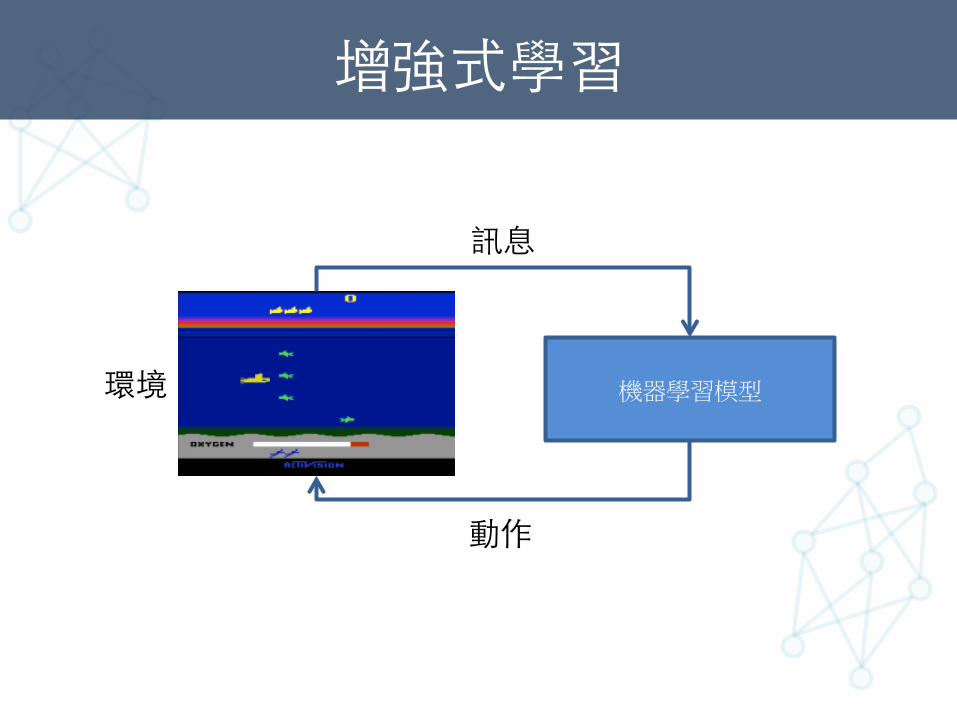
增強式學習
機器學習模型 環境
訊息
動作
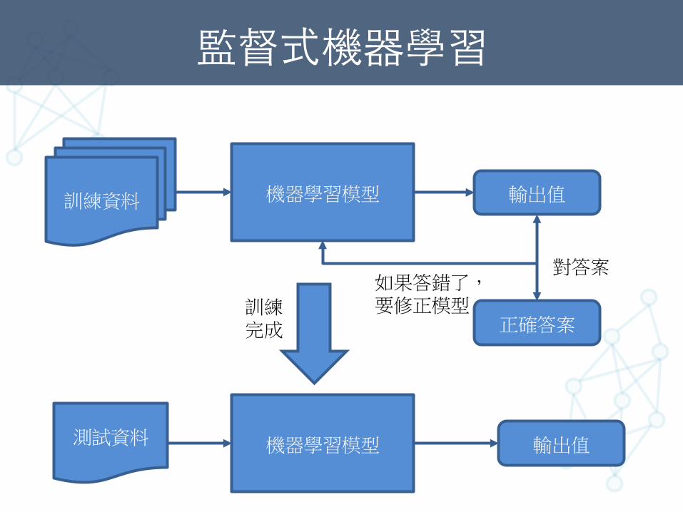
監督式機器學習
訓練資料 機器學習模型 輸出值
正確答案
對答案 如果答錯了,要修正模型
機器學習模型 測試資料
訓練完成
輸出值
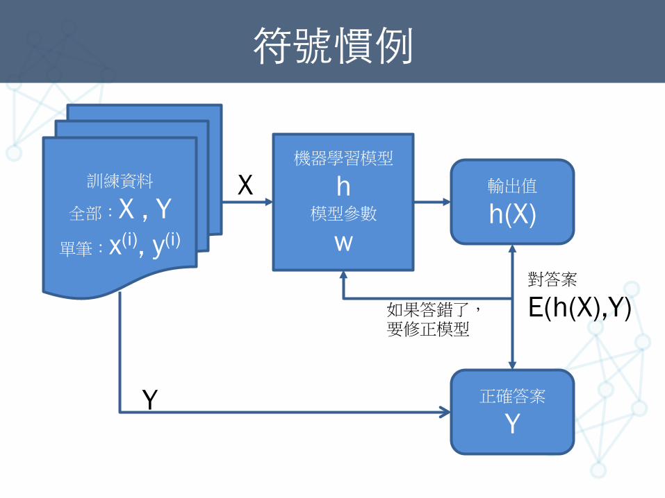
符號慣例
訓練資料
全部:X , Y 單筆:x(i), y(i)
機器學習模型
h 模型參數
w
輸出值
h(X)
正確答案
Y
對答案
E(h(X),Y) 如果答錯了,要修正模型
X
Y
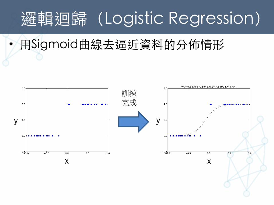
邏輯迴歸(Logistic Regression) • ⽤用Sigmoid曲線去逼近資料的分佈情形
x
y
x
y
訓練完成
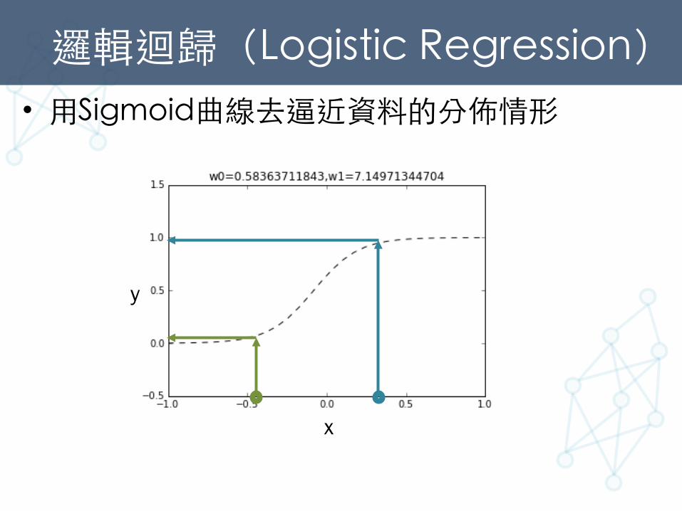
邏輯迴歸(Logistic Regression) • ⽤用Sigmoid曲線去逼近資料的分佈情形
x
y
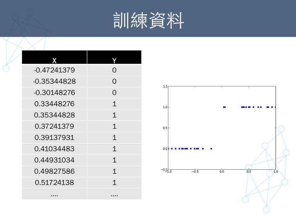
訓練資料
X Y -0.47241379 0 -0.35344828 0 -0.30148276 0 0.33448276 1 0.35344828 1 0.37241379 1 0.39137931 1 0.41034483 1 0.44931034 1 0.49827586 1 0.51724138 1
…. ….
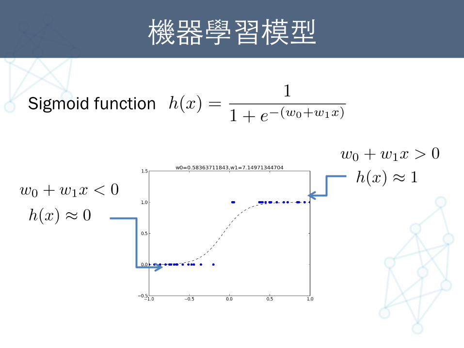
機器學習模型
Sigmoid function
w0 + w1x < 0
h(x) ⇡ 0
w0 + w1x > 0
h(x) ⇡ 1
h(x) =1
1 + e
�(w0+w1x)
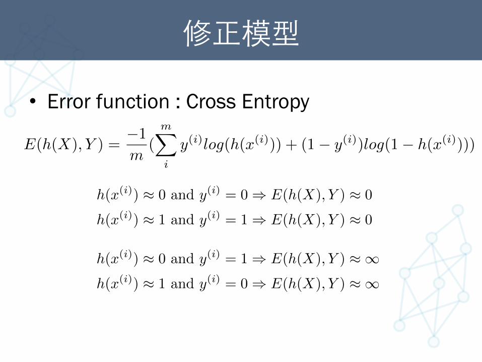
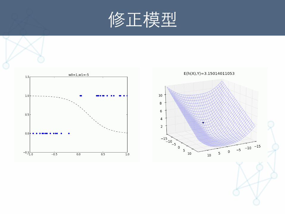
修正模型
• Error function : Cross Entropy
E(h(X), Y ) =�1
m
(mX
i
y
(i)log(h(x(i))) + (1� y
(i))log(1� h(x(i))))
h(x(i)) ⇡ 0 and y
(i) = 0 ) E(h(X), Y ) ⇡ 0
h(x(i)) ⇡ 1 and y
(i) = 1 ) E(h(X), Y ) ⇡ 0
h(x(i)) ⇡ 0 and y
(i) = 1 ) E(h(X), Y ) ⇡ 1h(x(i)) ⇡ 1 and y
(i) = 0 ) E(h(X), Y ) ⇡ 1
w1 w0
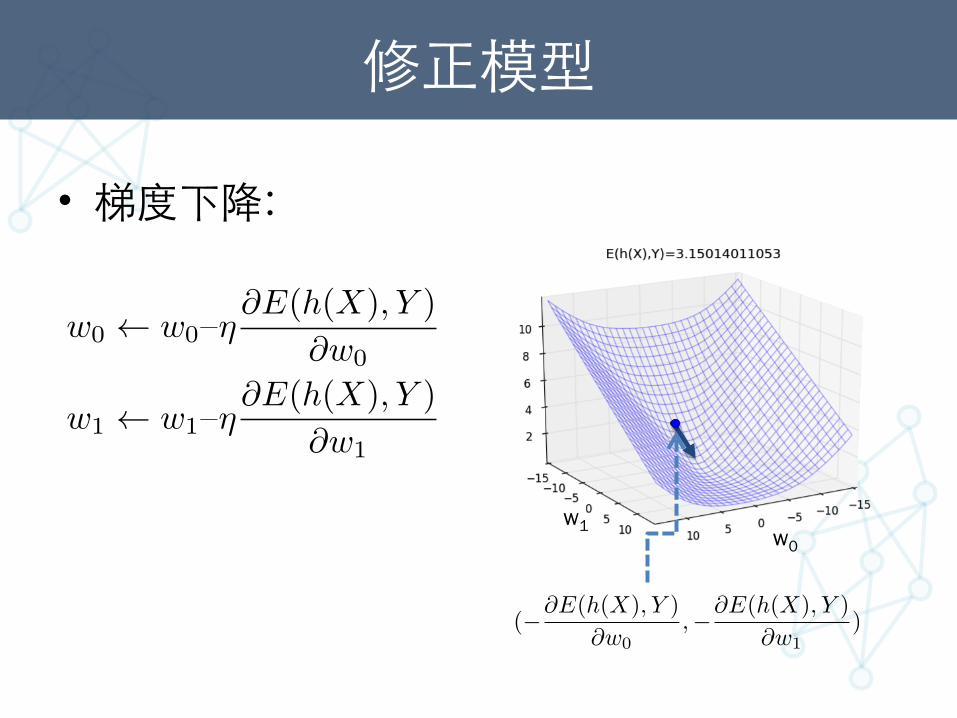
修正模型
• 梯度下降:
w0 w0–⌘
@E(h(X), Y )
@w0
w1 w1–⌘@E(h(X), Y )
@w1
(�@E(h(X), Y )
@w0,�@E(h(X), Y )
@w1)
修正模型
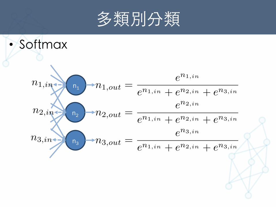
多類別分類 • Softmax
n1
n2
n3
n1,out =en1,in
en1,in + en2,in + en3,in
n2,out =en2,in
en1,in + en2,in + en3,in
n3,out =en3,in
en1,in + en2,in + en3,in
n1,in
n2,in
n3,in
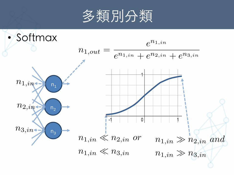
多類別分類 • Softmax
n1,out =en1,in
en1,in + en2,in + en3,in
n1
n2
n3
n1,in
n2,in
n3,in
n1,in � n2,in and
n1,in � n3,in
n1,in ⌧ n2,in or
n1,in ⌧ n3,in
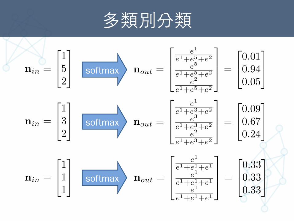
多類別分類
nin =
2
4132
3
5 nout
=
2
64
e
1
e
1+e
3+e
2
e
3
e
1+e
3+e
2
e
2
e
1+e
3+e
2
3
75 =
2
40.090.670.24
3
5
nin =
2
4111
3
5 nout
=
2
64
e
1
e
1+e
1+e
1
e
1
e
1+e
1+e
1
e
1
e
1+e
1+e
1
3
75 =
2
40.330.330.33
3
5
nout
=
2
64
e
1
e
1+e
5+e
2
e
5
e
1+e
5+e
2
e
2
e
1+e
5+e
2
3
75 =
2
40.010.940.05
3
5nin =
2
4152
3
5 softmax
softmax
softmax
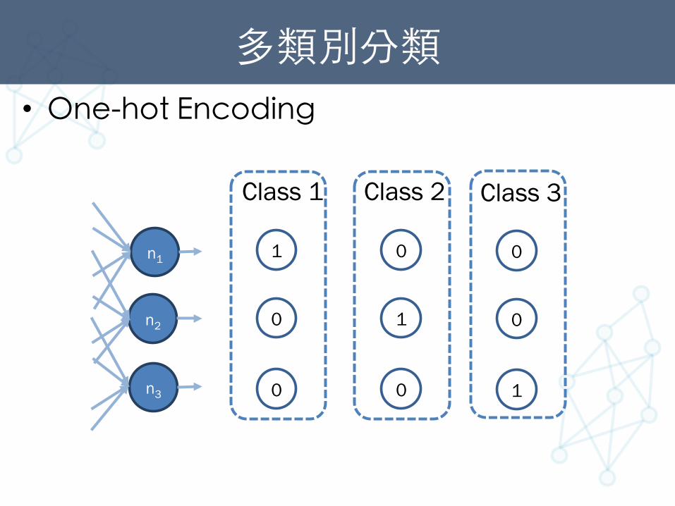
多類別分類 • One-hot Encoding
Class 1 Class 2 Class 3
1
0
0
0
1
0
0
0
1
n1
n2
n3
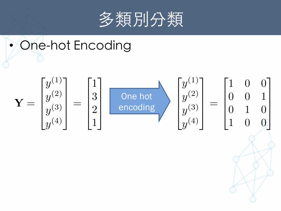
多類別分類 • One-hot Encoding
One hot encoding
2
664
y(1)
y(2)
y(3)
y(4)
3
775 =
2
664
1 0 00 0 10 1 01 0 0
3
775Y =
2
664
y(1)
y(2)
y(3)
y(4)
3
775 =
2
664
1321
3
775
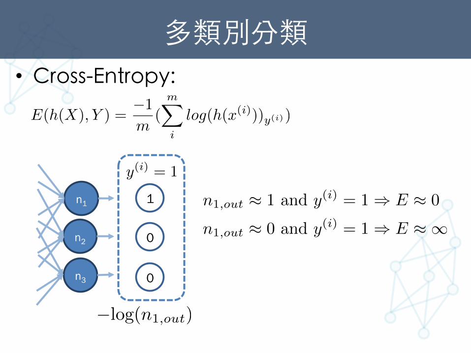
多類別分類 • Cross-Entropy:
1
0
0
n1
n2
n3
�log(n1,out)
E(h(X), Y ) =�1
m
(mX
i
log(h(x(i)))y(i))
y(i) = 1
n1,out ⇡ 1 and y(i) = 1 ) E ⇡ 0
n1,out ⇡ 0 and y(i) = 1 ) E ⇡ 1
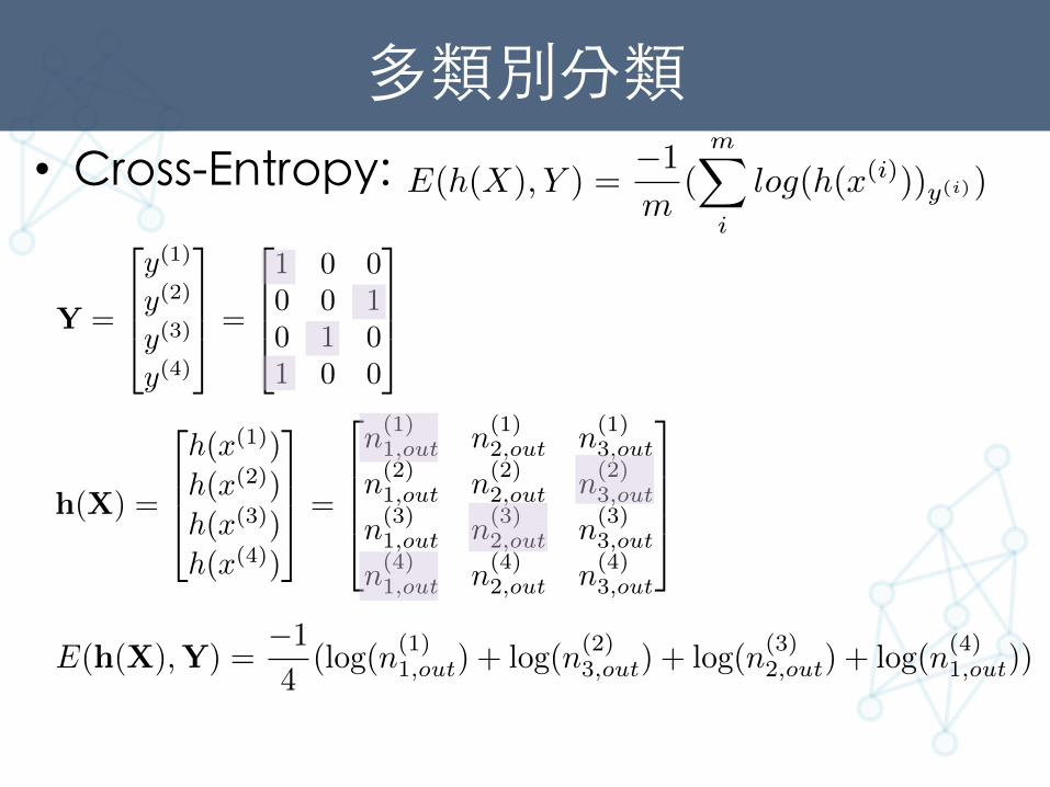
多類別分類 • Cross-Entropy:
E(h(X), Y ) =�1
m
(mX
i
log(h(x(i)))y(i))
E(h(X),Y) =
�1
4
(log(n(1)1,out) + log(n(2)
3,out) + log(n(3)2,out) + log(n(4)
1,out))
h(X) =
2
664
h(x(1))h(x(2))h(x(3))h(x(4))
3
775 =
2
6664
n
(1)1,out n
(1)2,out n
(1)3,out
n
(2)1,out n
(2)2,out n
(2)3,out
n
(3)1,out n
(3)2,out n
(3)3,out
n
(4)1,out n
(4)2,out n
(4)3,out
3
7775
Y =
2
664
y(1)
y(2)
y(3)
y(4)
3
775 =
2
664
1 0 00 0 10 1 01 0 0
3
775
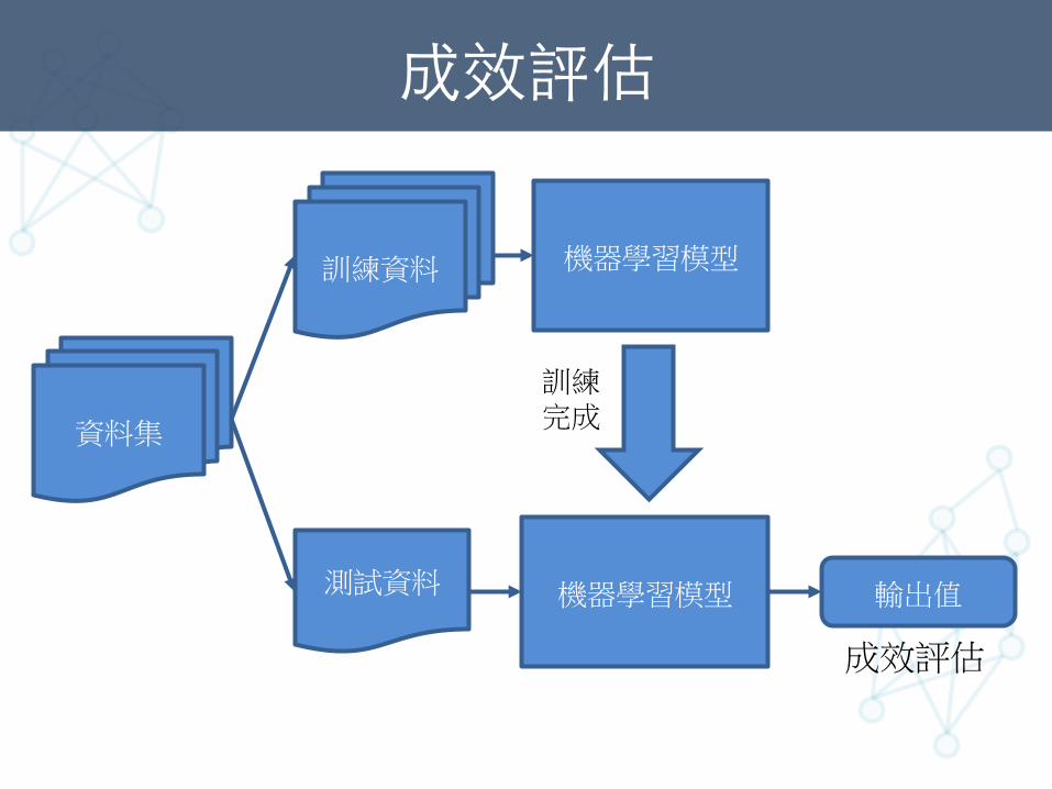
成效評估
訓練資料 機器學習模型
機器學習模型 測試資料
訓練完成
輸出值
資料集
成效評估
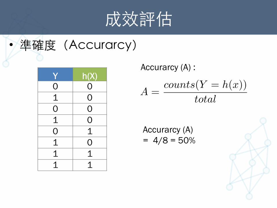
成效評估 • 準確度(Accurarcy)
Y h(X) 0 0 1 0 0 0 1 0 0 1 1 0 1 1 1 1
Accurarcy (A) :
A =counts(Y = h(x))
total
Accurarcy (A) = 4/8 = 50%
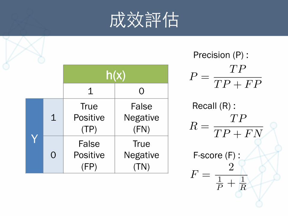
成效評估
h(x) 1 0
Y
1
True Positive
(TP)
False Negative
(FN) 0
False Positive
(FP)
True Negative
(TN)
P =TP
TP + FP
R =TP
TP + FN
F =2
1P + 1
R
Precision (P) :
Recall (R) :
F-score (F) :
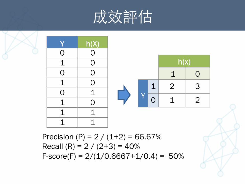
成效評估 Y h(X) 0 0 1 0 0 0 1 0 0 1 1 0 1 1 1 1
h(x) 1 0
Y
1 2 3
0 1 2
Precision (P) = 2 / (1+2) = 66.67% Recall (R) = 2 / (2+3) = 40% F-score(F) = 2/(1/0.6667+1/0.4) = 50%
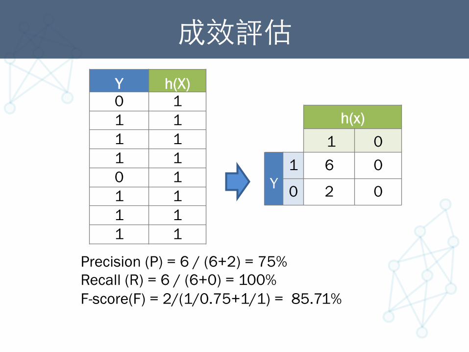
成效評估 Y h(X) 0 1 1 1 1 1 1 1 0 1 1 1 1 1 1 1
h(x) 1 0
Y
1 6 0
0 2 0
Precision (P) = 6 / (6+2) = 75% Recall (R) = 6 / (6+0) = 100% F-score(F) = 2/(1/0.75+1/1) = 85.71%
成效評估
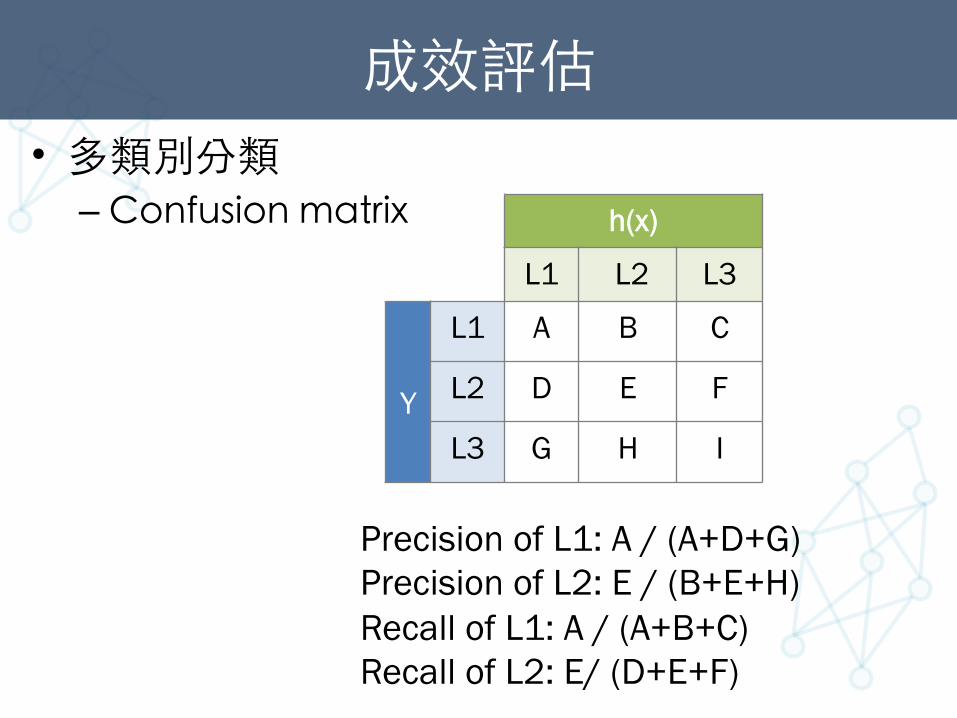
Precision of L1: A / (A+D+G) Precision of L2: E / (B+E+H) Recall of L1: A / (A+B+C) Recall of L2: E/ (D+E+F)
h(x)
L1 L2 L3
Y
L1 A B C
L2 D E F
L3 G H I
• 多類別分類 – Confusion matrix
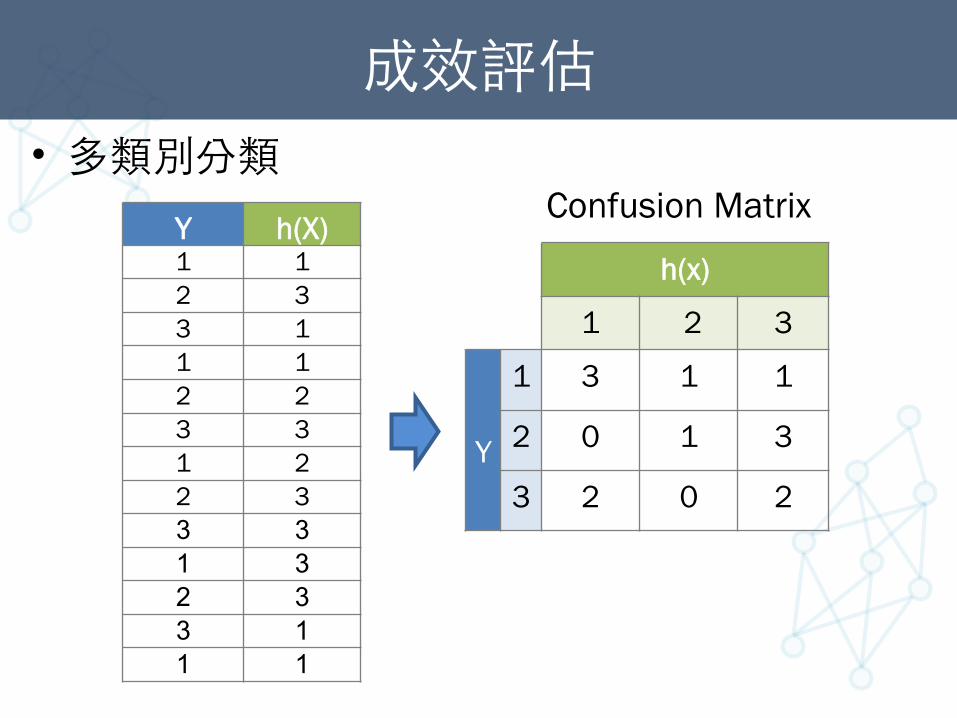
成效評估 • 多類別分類
Y h(X) 1 1 2 3 3 1 1 1 2 2 3 3 1 2 2 3 3 3 1 3 2 3 3 1 1 1
h(x)
1 2 3
Y
1 3 1 1
2 0 1 3
3 2 0 2
Confusion Matrix
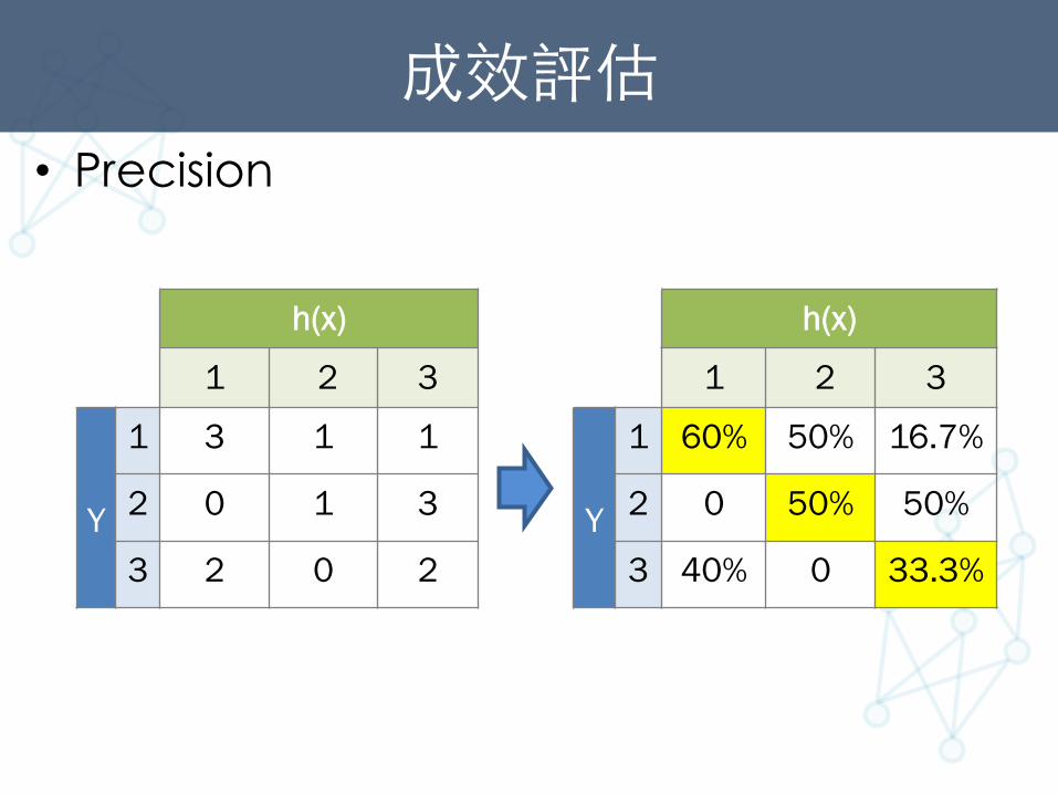
成效評估 • Precision
h(x)
1 2 3
Y
1 3 1 1
2 0 1 3
3 2 0 2
h(x)
1 2 3
Y
1 60% 50% 16.7%
2 0 50% 50%
3 40% 0 33.3%
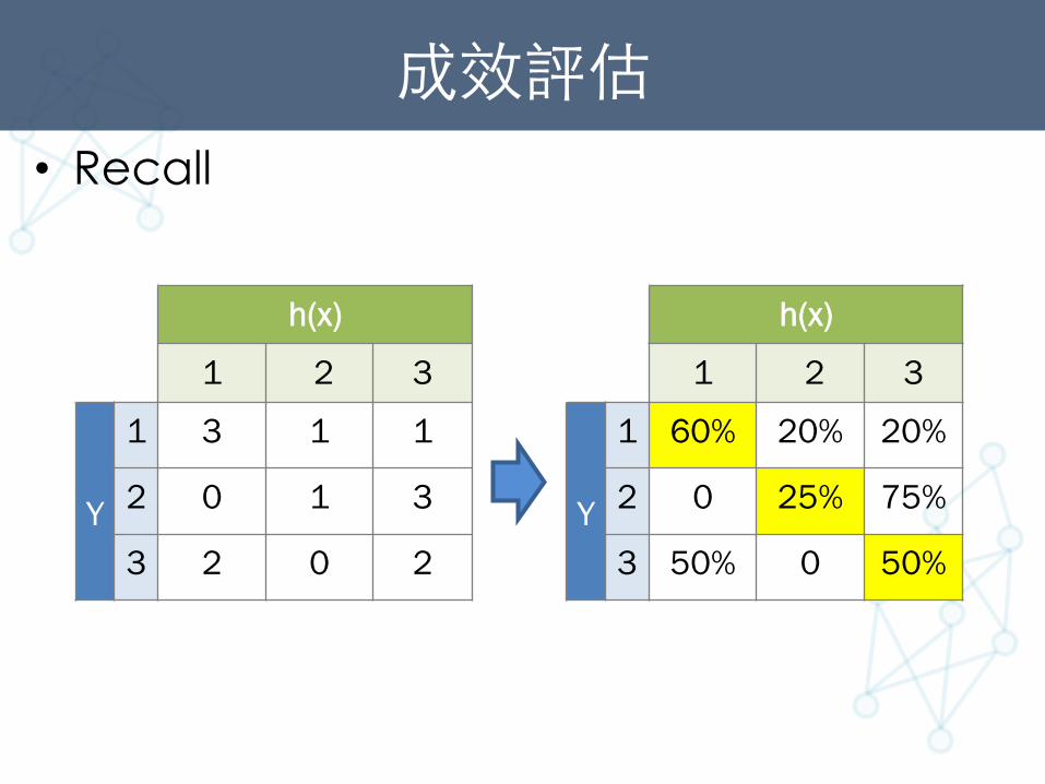
成效評估 • Recall
h(x)
1 2 3
Y
1 3 1 1
2 0 1 3
3 2 0 2
h(x)
1 2 3
Y
1 60% 20% 20%
2 0 25% 75%
3 50% 0 50%
Tensorflow簡介
Tensorflow
• https://www.tensorflow.org/ • TensorFlow 是 Google 開發的開源機器學習⼯工具。 • 透過使⽤用Computational Graph,來進⾏行數值演算。 • ⽀支援程式語⾔言:python、C++ • LICENSE: Apache 2.0 open source license • 系統需求:
– 作業系統必須為Mac或Linux – Python 2.7 或 3.3 (含以上)
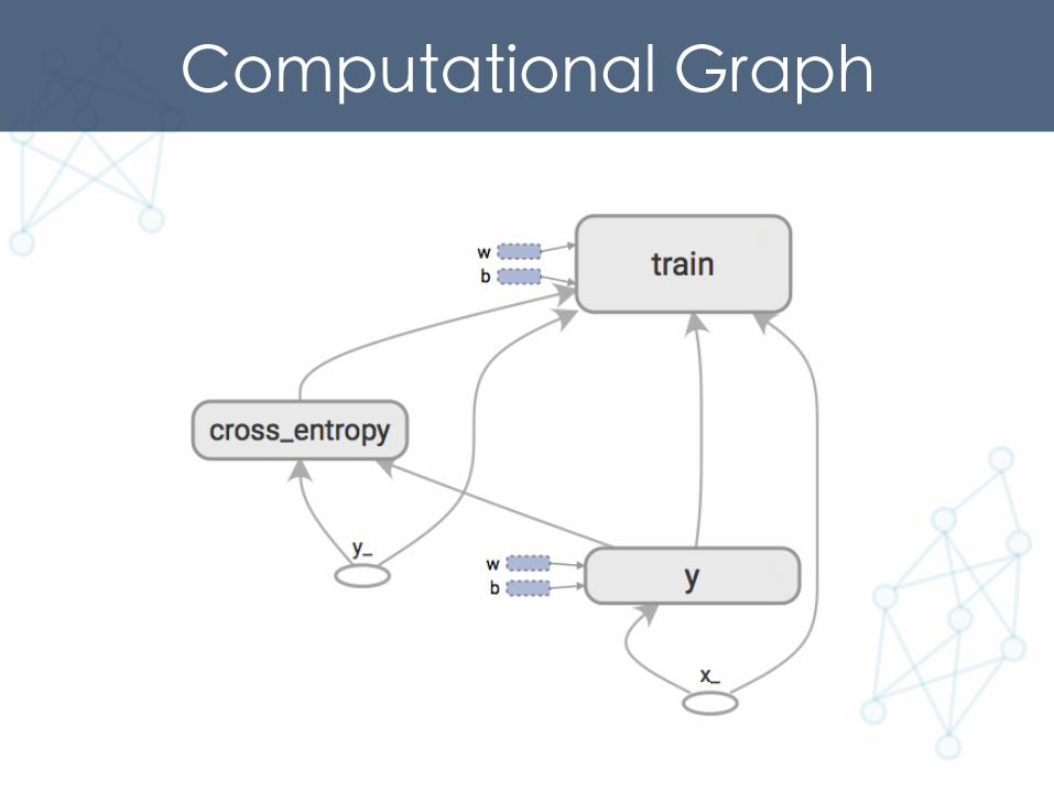
Computational Graph
Tensorflow
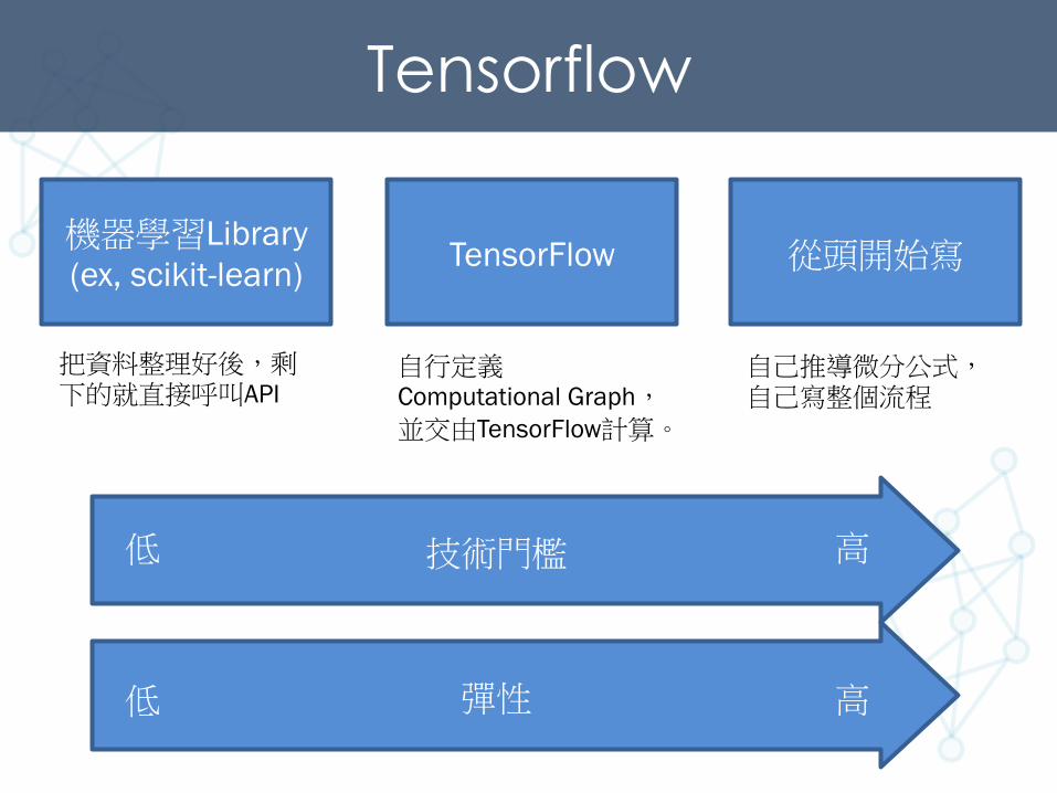
機器學習Library (ex, scikit-learn) TensorFlow 從頭開始寫
彈性
技術門檻
把資料整理好後,剩下的就直接呼叫API
自行定義Computational Graph,並交由TensorFlow計算。
自己推導微分公式,自己寫整個流程
低
低
高
高
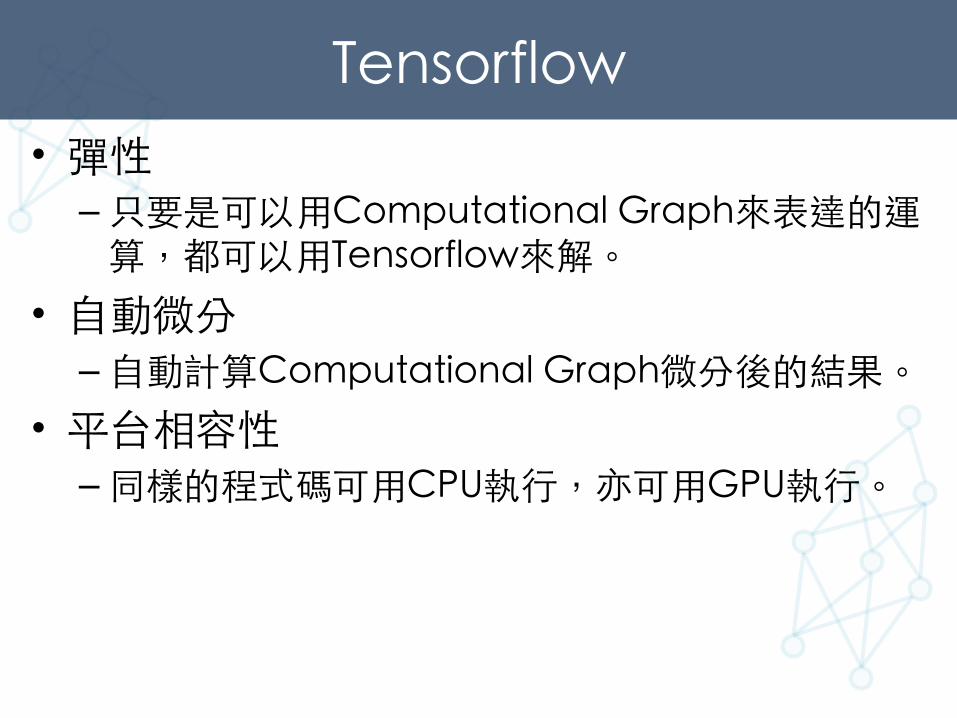
Tensorflow • 彈性
– 只要是可以⽤用Computational Graph來表達的運算,都可以⽤用Tensorflow來解。
• ⾃自動微分 – ⾃自動計算Computational Graph微分後的結果。
• 平台相容性 – 同樣的程式碼可⽤用CPU執⾏行,亦可⽤用GPU執⾏行。
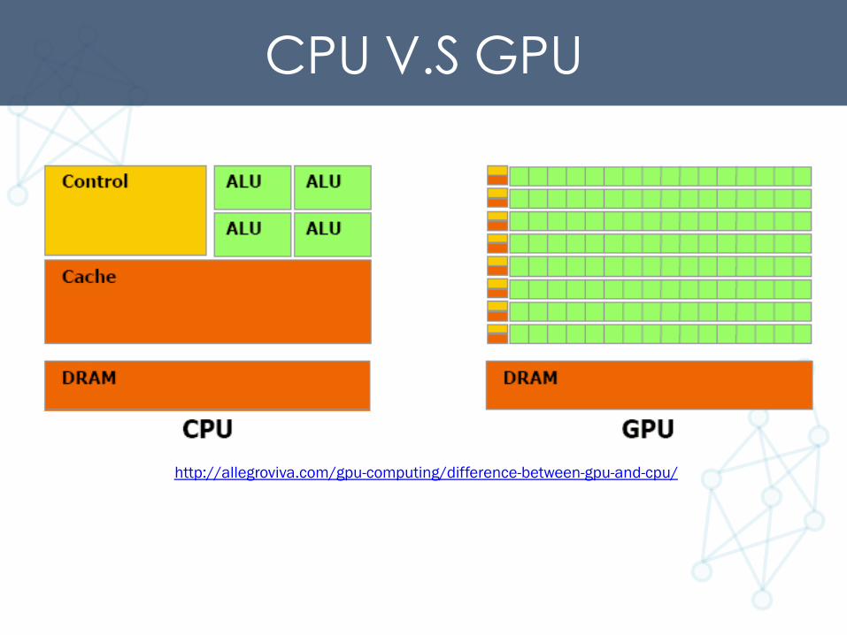
CPU V.S GPU
http://allegroviva.com/gpu-computing/difference-between-gpu-and-cpu/
Tensorflow安裝
Tensorflow安裝 • 1. 安裝pyenv • 2. 安裝anaconda-2.x.x • 3. 安裝tensorflow
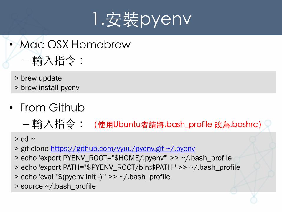
1.安裝pyenv • Mac OSX Homebrew
– 輸⼊入指令:
• From Github – 輸⼊入指令: (使⽤用Ubuntu者請將.bash_profile 改為.bashrc)
> cd ~ > git clone https://github.com/yyuu/pyenv.git ~/.pyenv > echo 'export PYENV_ROOT="$HOME/.pyenv"' >> ~/.bash_profile > echo 'export PATH="$PYENV_ROOT/bin:$PATH"' >> ~/.bash_profile > echo 'eval "$(pyenv init -)"' >> ~/.bash_profile > source ~/.bash_profile
> brew update > brew install pyenv
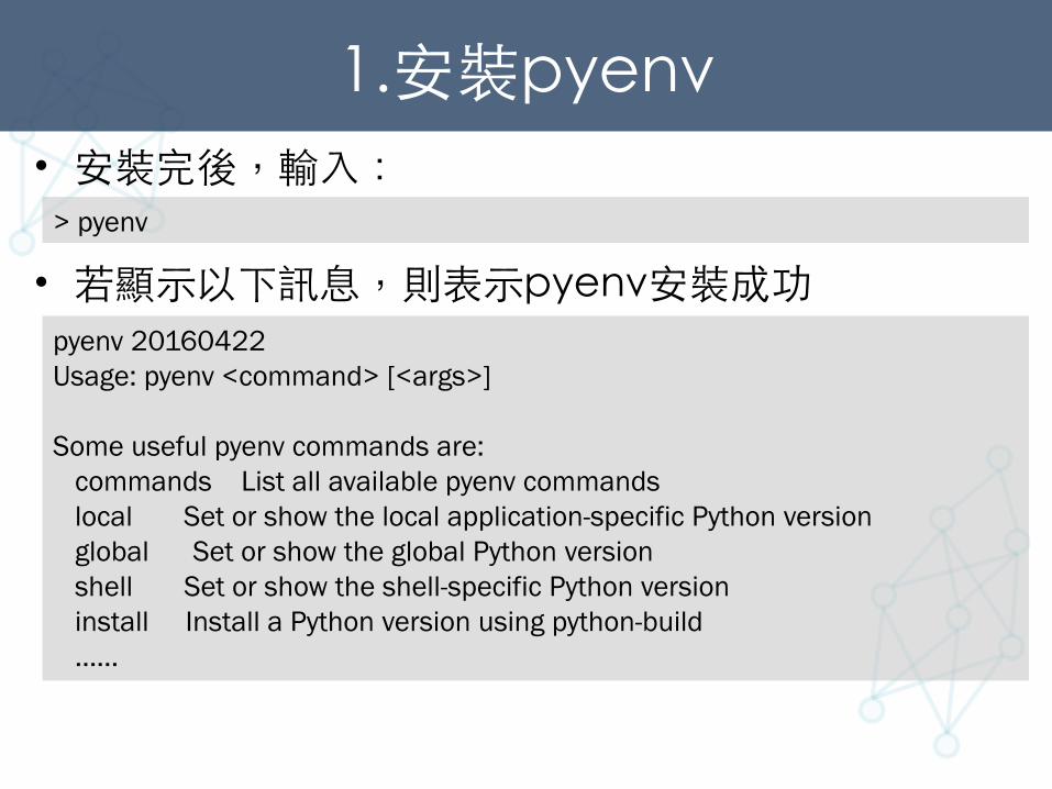
1.安裝pyenv • 安裝完後,輸⼊入:
• 若顯⽰示以下訊息,則表⽰示pyenv安裝成功 > pyenv
pyenv 20160422 Usage: pyenv <command> [<args>] Some useful pyenv commands are: commands List all available pyenv commands local Set or show the local application-specific Python version global Set or show the global Python version shell Set or show the shell-specific Python version install Install a Python version using python-build ……
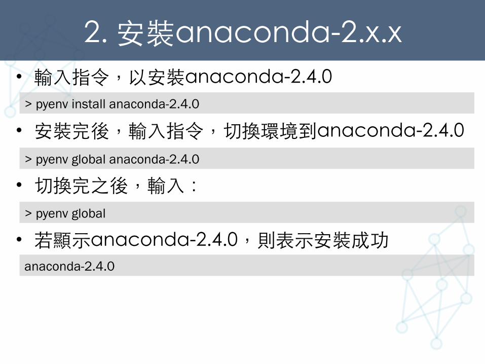
2. 安裝anaconda-2.x.x • 輸⼊入指令,以安裝anaconda-2.4.0
• 安裝完後,輸⼊入指令,切換環境到anaconda-2.4.0
• 切換完之後,輸⼊入:
• 若顯⽰示anaconda-2.4.0,則表⽰示安裝成功
> pyenv install anaconda-2.4.0
> pyenv global anaconda-2.4.0
> pyenv global
anaconda-2.4.0
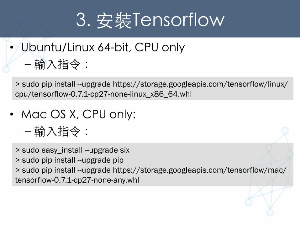
3. 安裝Tensorflow • Ubuntu/Linux 64-bit, CPU only
– 輸⼊入指令: • Mac OS X, CPU only:
– 輸⼊入指令:
> sudo pip install --upgrade https://storage.googleapis.com/tensorflow/linux/cpu/tensorflow-0.7.1-cp27-none-linux_x86_64.whl
> sudo easy_install --upgrade six > sudo pip install --upgrade pip > sudo pip install --upgrade https://storage.googleapis.com/tensorflow/mac/tensorflow-0.7.1-cp27-none-any.whl
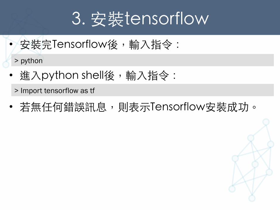
3. 安裝tensorflow • 安裝完Tensorflow後,輸⼊入指令: • 進⼊入python shell後,輸⼊入指令:
• 若無任何錯誤訊息,則表⽰示Tensorflow安裝成功。
> python
> Import tensorflow as tf

單層感知器實作
單層感知器實作 https://github.com/ckmarkoh/ntc_deeplearning_tensorflow/blob/master/sec1/mnist_train.ipynb
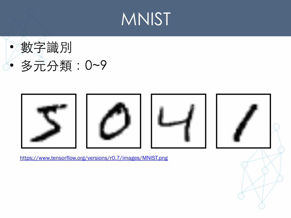
MNIST • 數字識別 • 多元分類:0~9
https://www.tensorflow.org/versions/r0.7/images/MNIST.png
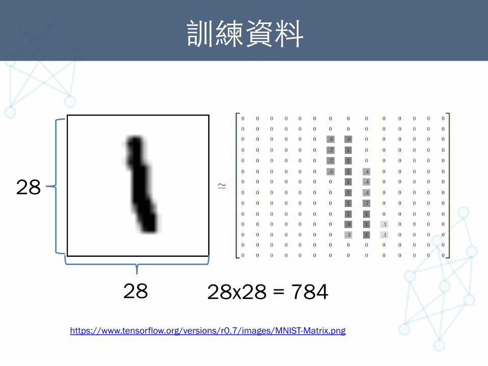
訓練資料
https://www.tensorflow.org/versions/r0.7/images/MNIST-Matrix.png
28x28 = 784
28
28
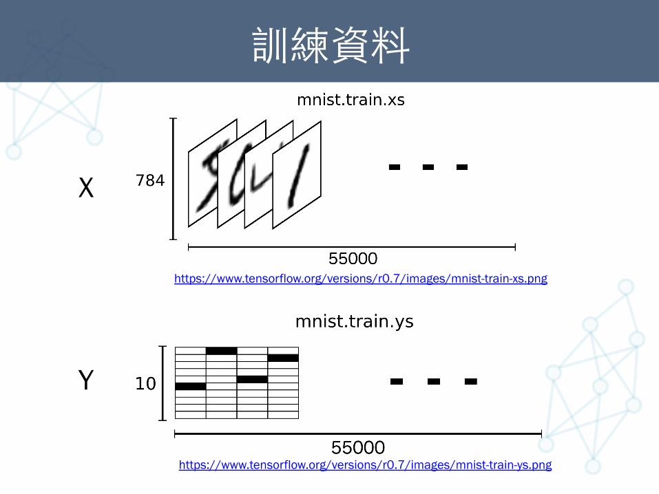
訓練資料
https://www.tensorflow.org/versions/r0.7/images/mnist-train-xs.png
https://www.tensorflow.org/versions/r0.7/images/mnist-train-ys.png
X
Y
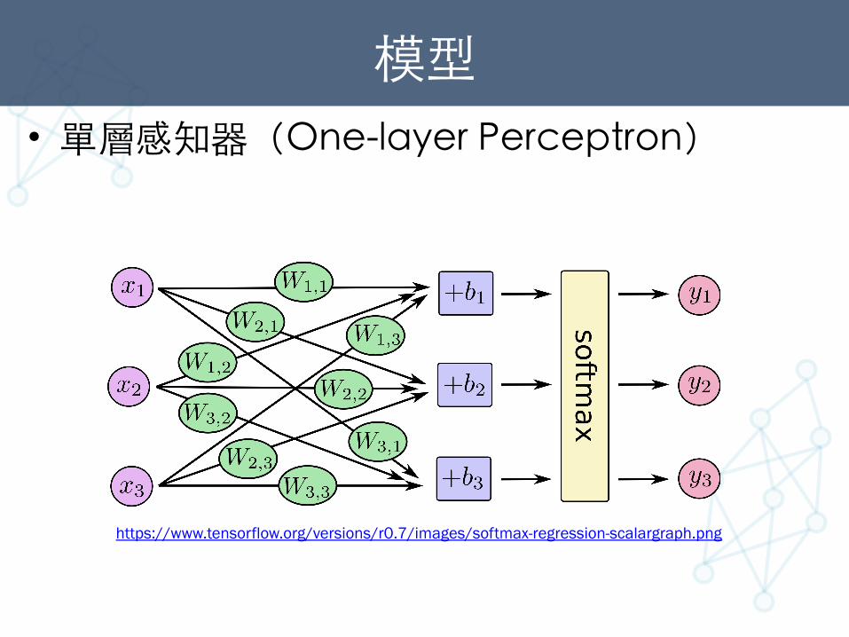
模型 • 單層感知器(One-layer Perceptron)
https://www.tensorflow.org/versions/r0.7/images/softmax-regression-scalargraph.png
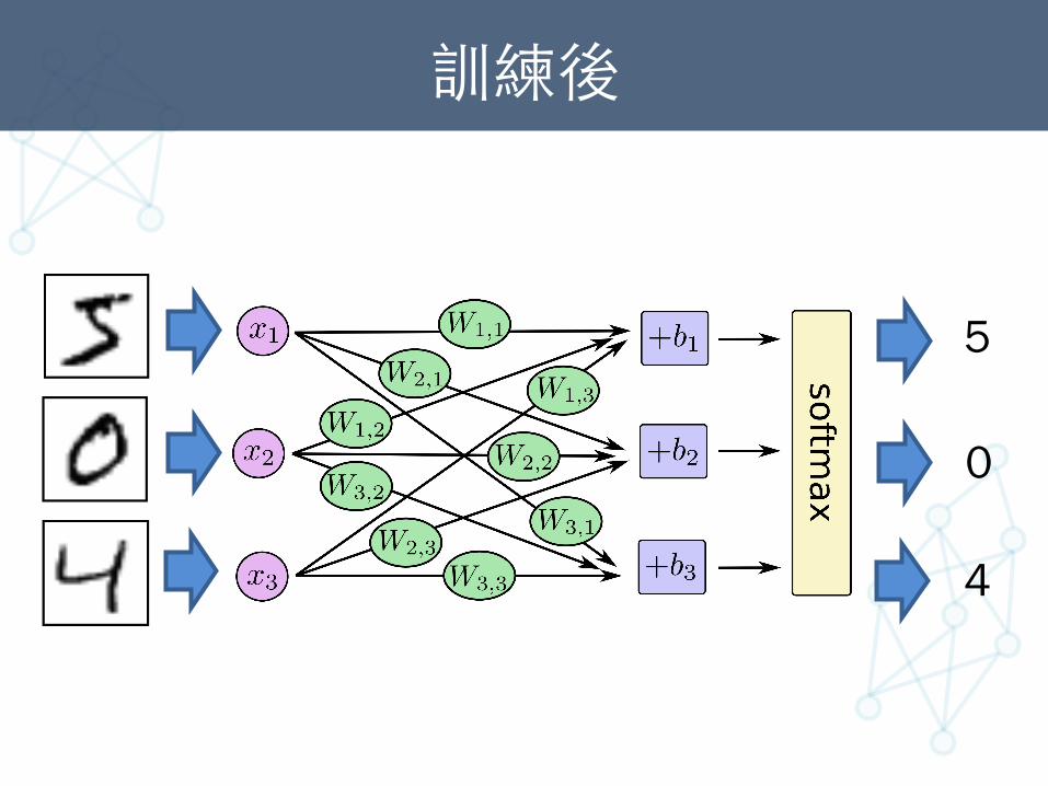
訓練後
5
0
4
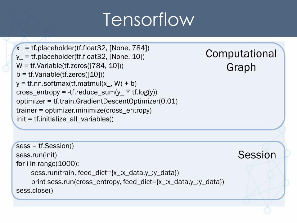
Tensorflow x_ = tf.placeholder(tf.float32, [None, 784]) y_ = tf.placeholder(tf.float32, [None, 10]) W = tf.Variable(tf.zeros([784, 10])) b = tf.Variable(tf.zeros([10])) y = tf.nn.softmax(tf.matmul(x_, W) + b) cross_entropy = -tf.reduce_sum(y_ * tf.log(y)) optimizer = tf.train.GradientDescentOptimizer(0.01) trainer = optimizer.minimize(cross_entropy) init = tf.initialize_all_variables() sess = tf.Session() sess.run(init) for i in range(1000):
sess.run(train, feed_dict={x_:x_data,y_:y_data}) print sess.run(cross_entropy, feed_dict={x_:x_data,y_:y_data})
sess.close()
Computational Graph
Session
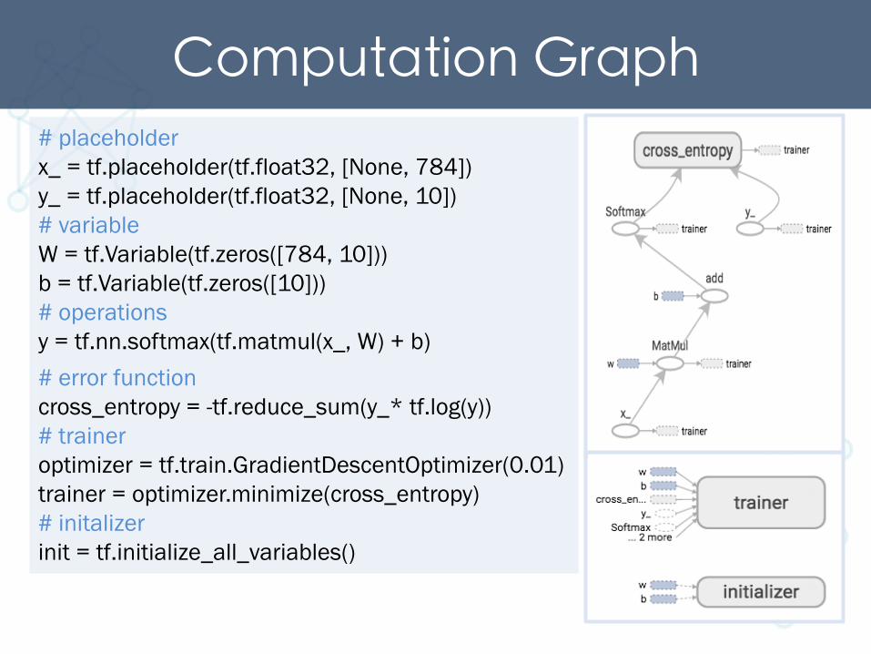
Computation Graph # placeholder x_ = tf.placeholder(tf.float32, [None, 784]) y_ = tf.placeholder(tf.float32, [None, 10])
# variable W = tf.Variable(tf.zeros([784, 10])) b = tf.Variable(tf.zeros([10])) # operations y = tf.nn.softmax(tf.matmul(x_, W) + b)
# error function cross_entropy = -tf.reduce_sum(y_* tf.log(y)) # trainer optimizer = tf.train.GradientDescentOptimizer(0.01) trainer = optimizer.minimize(cross_entropy) # initalizer init = tf.initialize_all_variables()
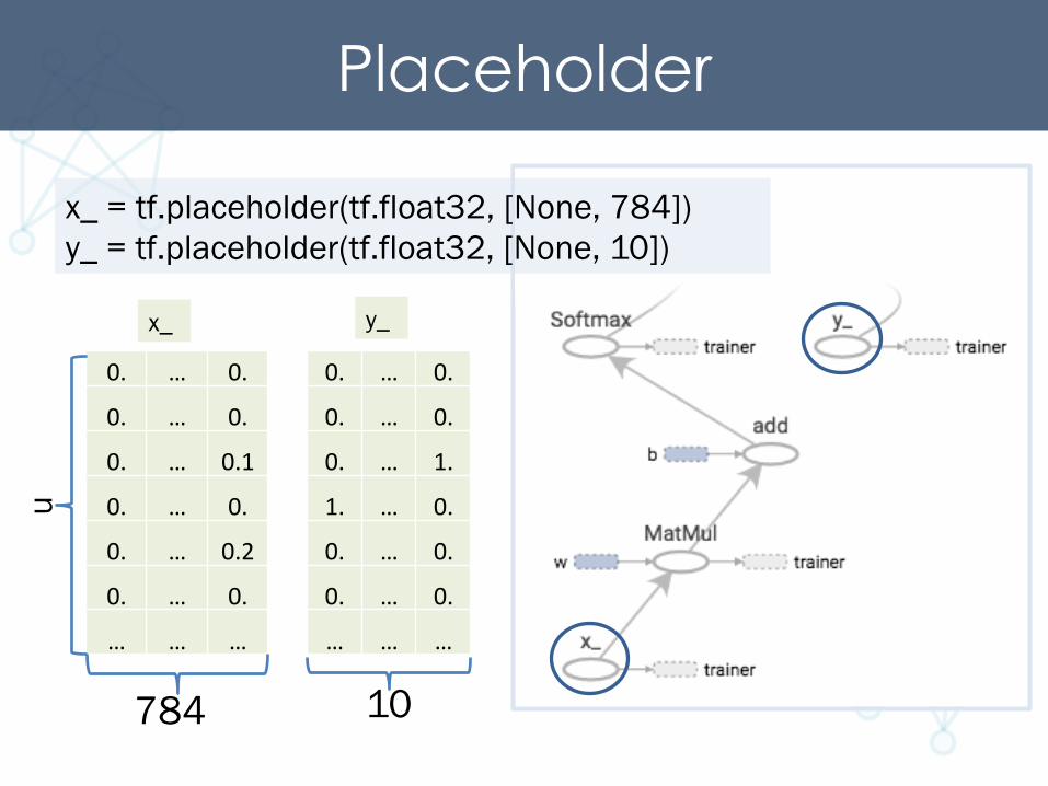
Placeholder
0. … 0.
0. … 0.
0. … 0.1
0. … 0.
0. … 0.2
0. … 0.
… … …
x_ y_
x_ = tf.placeholder(tf.float32, [None, 784]) y_ = tf.placeholder(tf.float32, [None, 10])
0. … 0.
0. … 0.
0. … 1.
1. … 0.
0. … 0.
0. … 0.
… … …
784 10
n
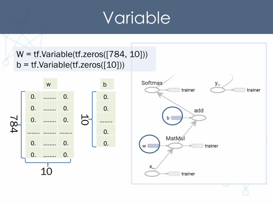
Variable
W = tf.Variable(tf.zeros([784, 10])) b = tf.Variable(tf.zeros([10]))
b w
0. …….. 0.
0. …….. 0.
0. …….. 0.
…….. …….. ……..
0. …….. 0.
0. …….. 0.
0.
0.
……..
0.
0.
784
10 10
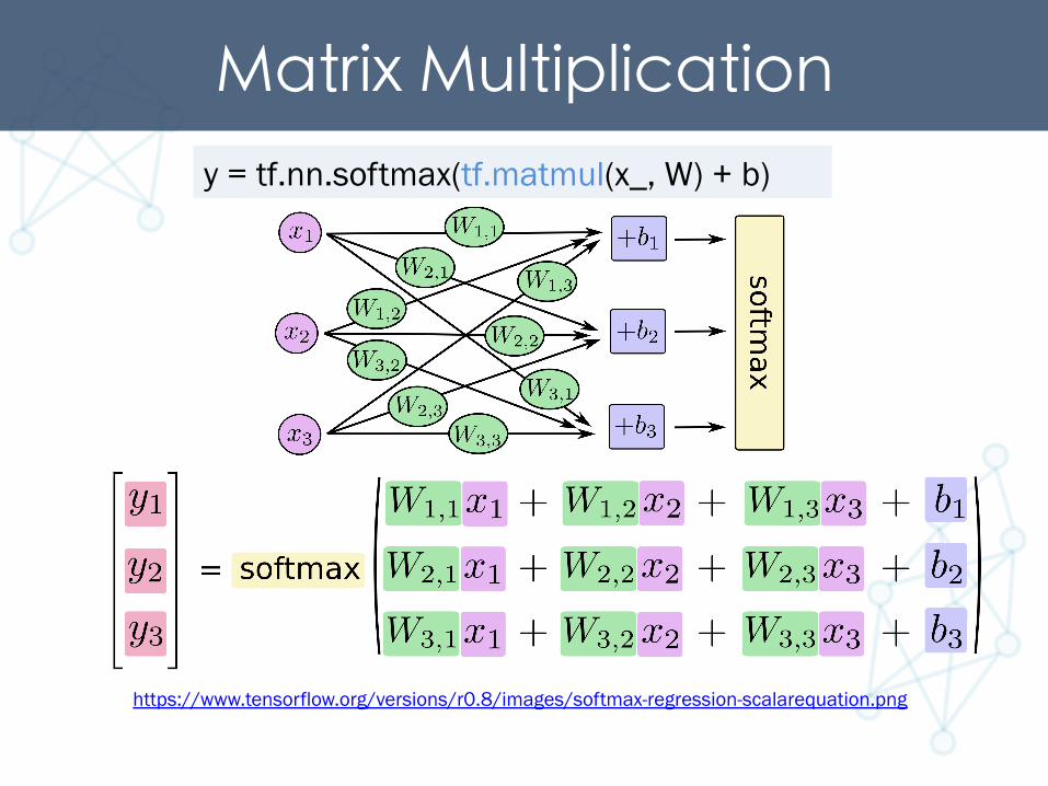
Matrix Multiplication y = tf.nn.softmax(tf.matmul(x_, W) + b)
https://www.tensorflow.org/versions/r0.8/images/softmax-regression-scalarequation.png
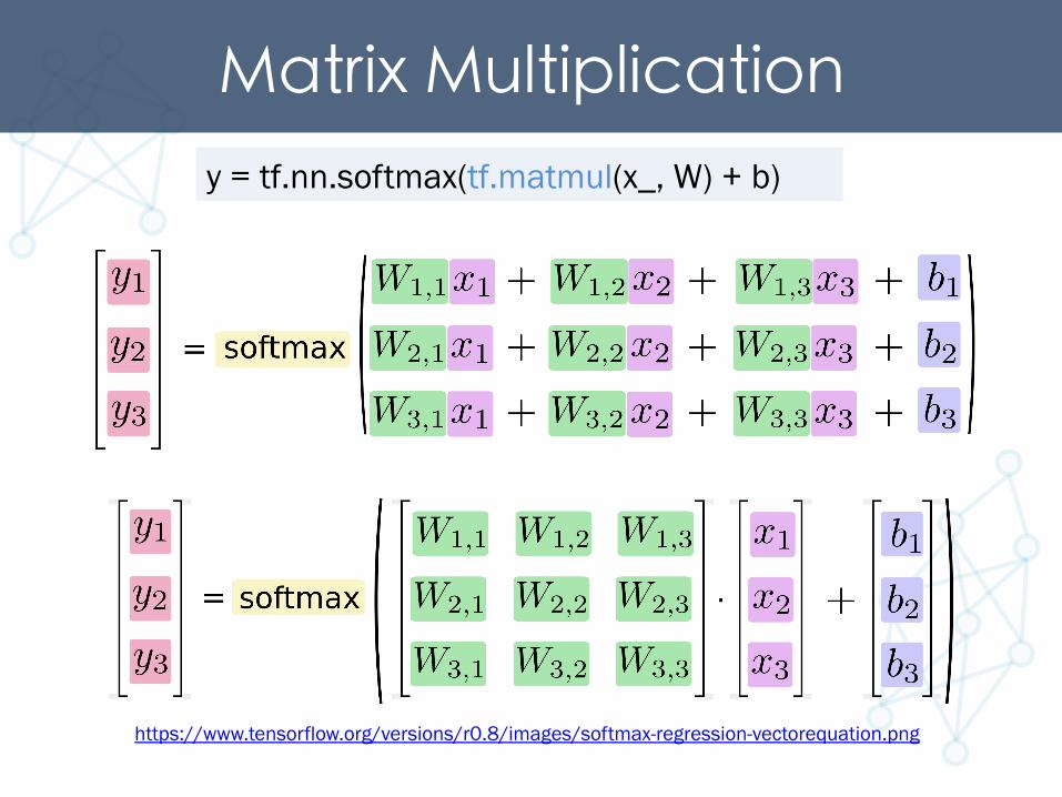
Matrix Multiplication y = tf.nn.softmax(tf.matmul(x_, W) + b)
https://www.tensorflow.org/versions/r0.8/images/softmax-regression-vectorequation.png
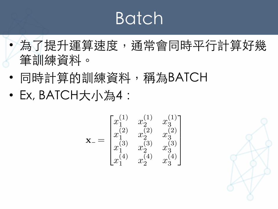
Batch • 為了提升運算速度,通常會同時平⾏行計算好幾
筆訓練資料。 • 同時計算的訓練資料,稱為BATCH • Ex, BATCH⼤大⼩小為4:
x =
2
6664
x
(1)1 x
(1)2 x
(1)3
x
(2)1 x
(2)2 x
(2)3
x
(3)1 x
(3)2 x
(3)3
x
(4)1 x
(4)2 x
(4)3
3
7775
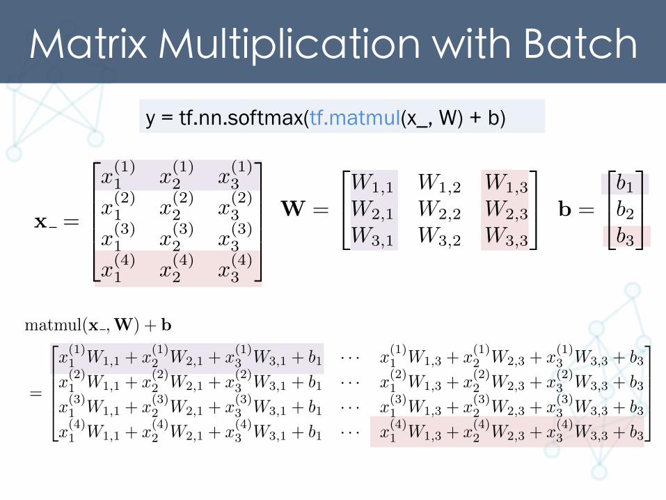
Matrix Multiplication with Batch y = tf.nn.softmax(tf.matmul(x_, W) + b)
x =
2
6664
x
(1)1 x
(1)2 x
(1)3
x
(2)1 x
(2)2 x
(2)3
x
(3)1 x
(3)2 x
(3)3
x
(4)1 x
(4)2 x
(4)3
3
7775W =
2
4W1,1 W1,2 W1,3
W2,1 W2,2 W2,3
W3,1 W3,2 W3,3
3
5 b =
2
4b1b2b3
3
5
matmul(x ,W) + b
=
2
6664
x
(1)1 W1,1 + x
(1)2 W2,1 + x
(1)3 W3,1 + b1 · · · x
(1)1 W1,3 + x
(1)2 W2,3 + x
(1)3 W3,3 + b3
x
(2)1 W1,1 + x
(2)2 W2,1 + x
(2)3 W3,1 + b1 · · · x
(2)1 W1,3 + x
(2)2 W2,3 + x
(2)3 W3,3 + b3
x
(3)1 W1,1 + x
(3)2 W2,1 + x
(3)3 W3,1 + b1 · · · x
(3)1 W1,3 + x
(3)2 W2,3 + x
(3)3 W3,3 + b3
x
(4)1 W1,1 + x
(4)2 W2,1 + x
(4)3 W3,1 + b1 · · · x
(4)1 W1,3 + x
(4)2 W2,3 + x
(4)3 W3,3 + b3
3
7775
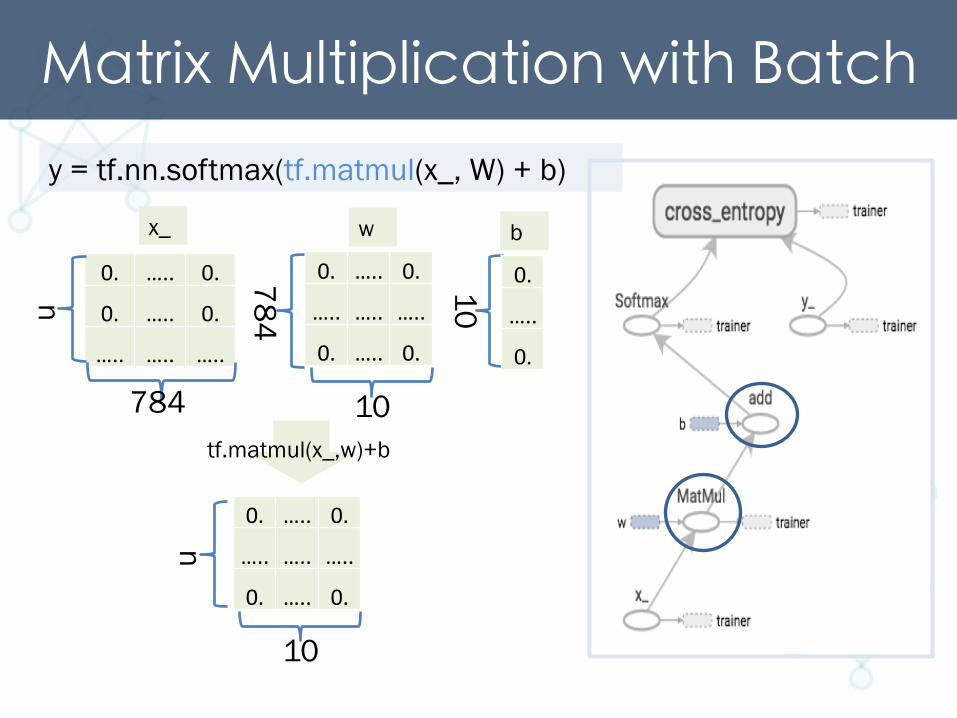
Matrix Multiplication with Batch y = tf.nn.softmax(tf.matmul(x_, W) + b)
w x_
tf.matmul(x_,w)+b
b
0. ….. 0.
0. ….. 0.
….. ….. …..
784
0. ….. 0.
….. ….. …..
0. ….. 0.
10
10
0.
…..
0.
784
n
0. ….. 0.
….. ….. …..
0. ….. 0.
10
n
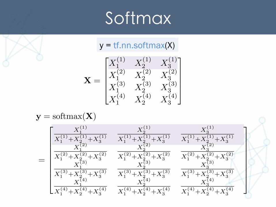
Softmax y = tf.nn.softmax(X)
X =
2
6664
X(1)1 X(1)
2 X(1)3
X(2)1 X(2)
2 X(2)3
X(3)1 X(3)
2 X(3)3
X(4)1 X(4)
2 X(4)3
3
7775
y = softmax(X)
=
2
66666664
X(1)1
X(1)1 +X(1)
2 +X(1)3
X(1)2
X(1)1 +X(1)
2 +X(1)3
X(1)3
X(1)1 +X(1)
2 +X(1)3
X(2)1
X(2)1 +X(2)
2 +X(2)3
X(2)2
X(2)1 +X(2)
2 +X(2)3
X(2)3
X(2)1 +X(2)
2 +X(2)3
X(3)1
X(3)1 +X(3)
2 +X(3)3
X(3)2
X(3)1 +X(3)
2 +X(3)3
X(3)3
X(3)1 +X(3)
2 +X(3)3
X(4)1
X(4)1 +X(4)
2 +X(4)3
X(4)2
X(4)1 +X(4)
2 +X(4)3
X(4)3
X(4)1 +X(4)
2 +X(4)3
3
77777775
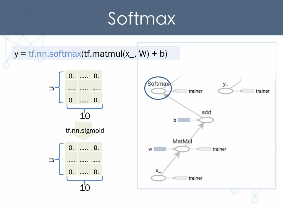
Softmax y = tf.nn.softmax(tf.matmul(x_, W) + b)
tf.nn.sigmoid
0. ….. 0.
….. ….. …..
0. ….. 0.
10
n
0. ….. 0.
….. ….. …..
0. ….. 0.
10
n
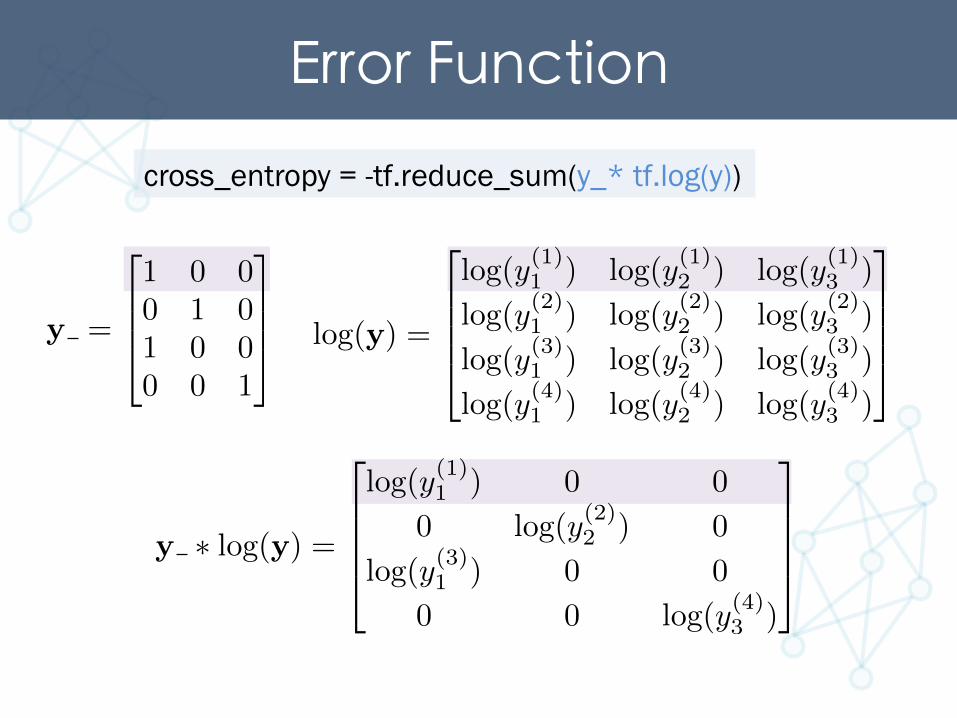
Error Function cross_entropy = -tf.reduce_sum(y_* tf.log(y))
y =
2
664
1 0 00 1 01 0 00 0 1
3
775 log(y) =
2
6664
log(y(1)1 ) log(y(1)2 ) log(y(1)3 )
log(y(2)1 ) log(y(2)2 ) log(y(2)3 )
log(y(3)1 ) log(y(3)2 ) log(y(3)3 )
log(y(4)1 ) log(y(4)2 ) log(y(4)3 )
3
7775
y ⇤ log(y) =
2
6664
log(y(1)1 ) 0 0
0 log(y(2)2 ) 0
log(y(3)1 ) 0 0
0 0 log(y(4)3 )
3
7775
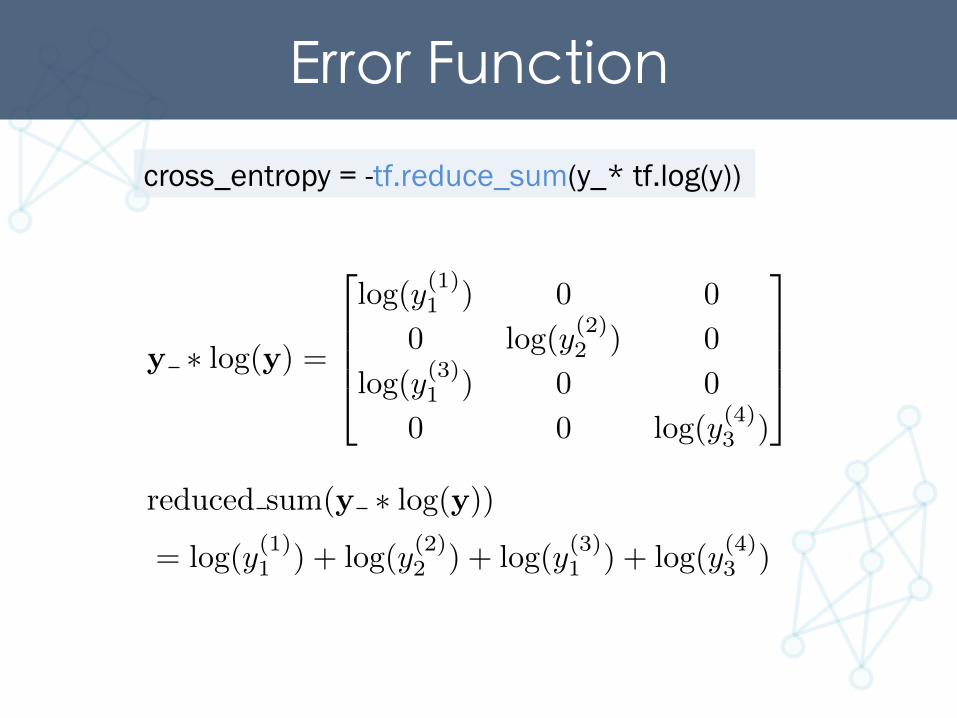
Error Function cross_entropy = -tf.reduce_sum(y_* tf.log(y))
y ⇤ log(y) =
2
6664
log(y(1)1 ) 0 0
0 log(y(2)2 ) 0
log(y(3)1 ) 0 0
0 0 log(y(4)3 )
3
7775
reduced sum(y ⇤ log(y))
= log(y(1)1 ) + log(y(2)2 ) + log(y(3)1 ) + log(y(4)3 )
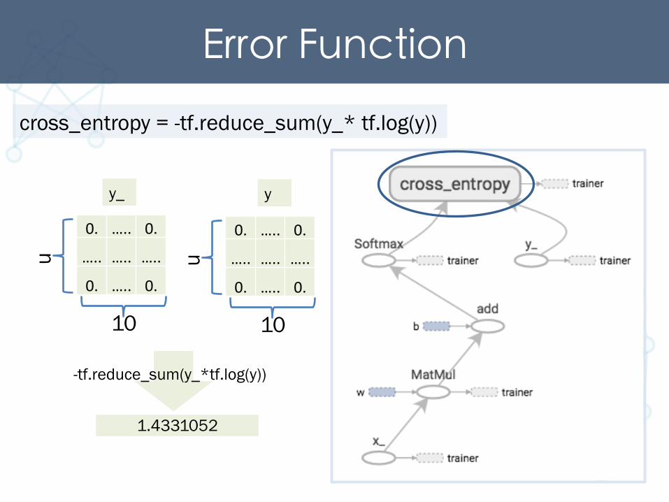
Error Function cross_entropy = -tf.reduce_sum(y_* tf.log(y))
y_ y
1.4331052
-tf.reduce_sum(y_*tf.log(y))
0. ….. 0.
….. ….. …..
0. ….. 0.
10
n
0. ….. 0.
….. ….. …..
0. ….. 0.
10
n
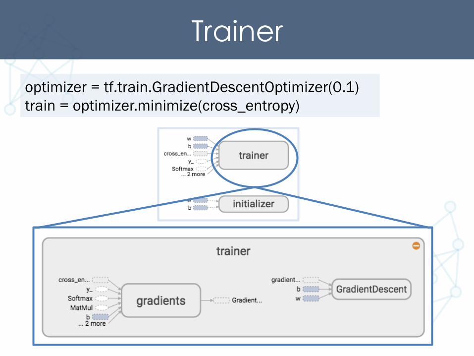
Trainer optimizer = tf.train.GradientDescentOptimizer(0.1) train = optimizer.minimize(cross_entropy)
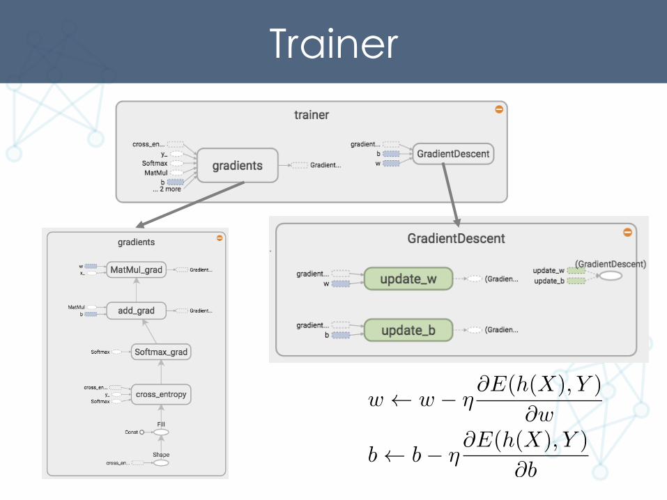
Trainer
w w � ⌘@E(h(X), Y )
@w
b b� ⌘@E(h(X), Y )
@b
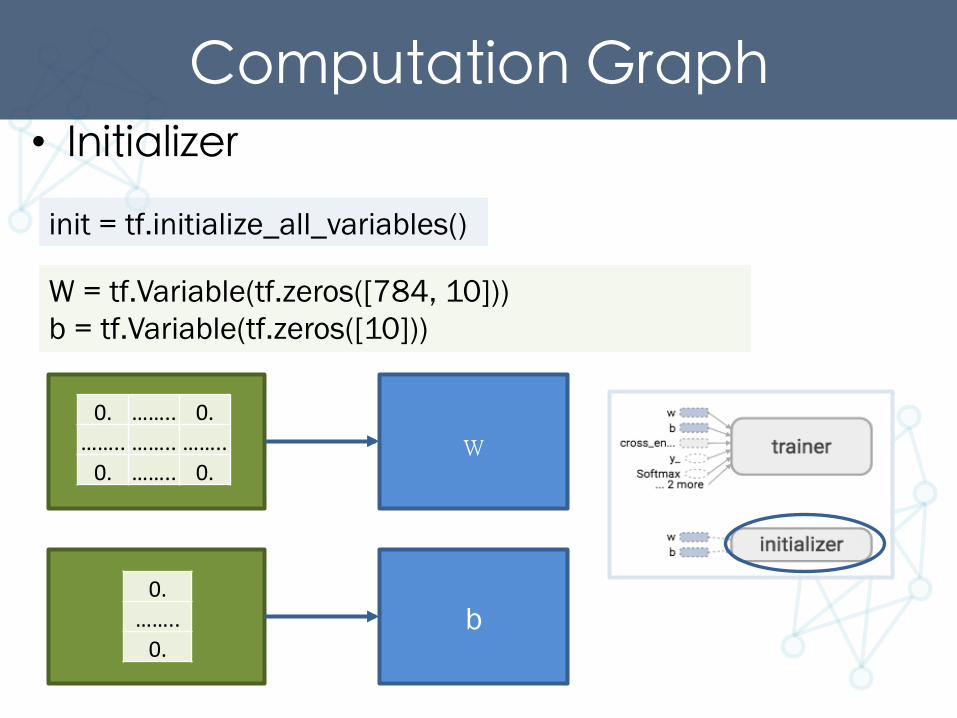
Computation Graph • Initializer
init = tf.initialize_all_variables()
w
b
W = tf.Variable(tf.zeros([784, 10])) b = tf.Variable(tf.zeros([10]))
0. …….. 0. …….. …….. …….. 0. …….. 0.
0. …….. 0.
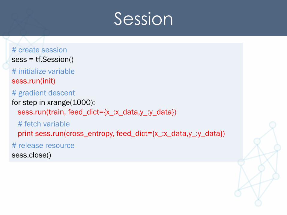
Session # create session sess = tf.Session()
# initialize variable sess.run(init)
# gradient descent for step in xrange(1000): sess.run(train, feed_dict={x_:x_data,y_:y_data})
# fetch variable print sess.run(cross_entropy, feed_dict={x_:x_data,y_:y_data})
# release resource sess.close()
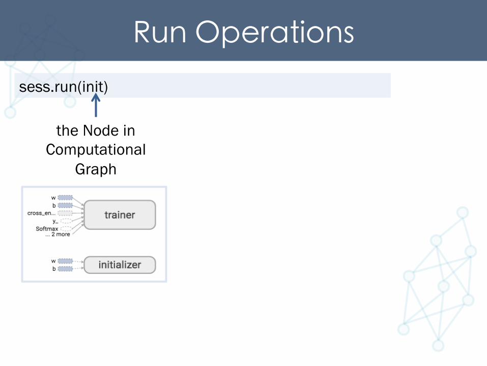
Run Operations sess.run(init)
the Node in Computational
Graph
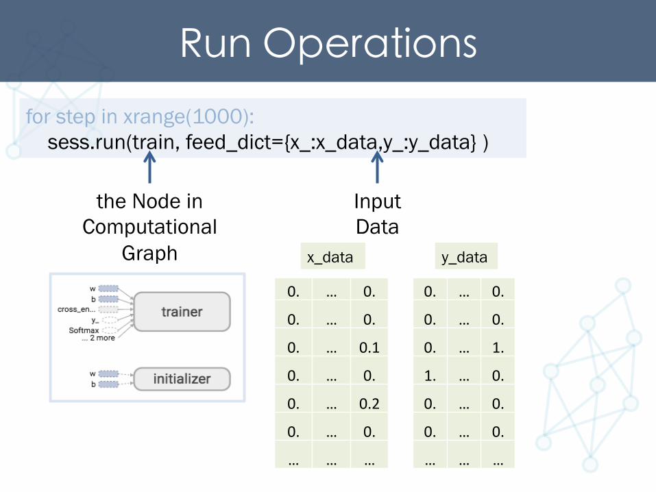
Run Operations for step in xrange(1000): sess.run(train, feed_dict={x_:x_data,y_:y_data} )
the Node in Computational
Graph
Input Data
x_data y_data
0. … 0.
0. … 0.
0. … 0.1
0. … 0.
0. … 0.2
0. … 0.
… … …
0. … 0.
0. … 0.
0. … 1.
1. … 0.
0. … 0.
0. … 0.
… … …
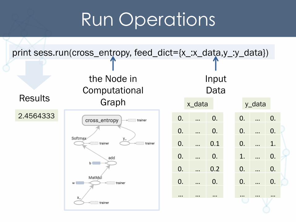
Run Operations print sess.run(cross_entropy, feed_dict={x_:x_data,y_:y_data})
the Node in Computational
Graph
Input Data
x_data y_data Results
2.4564333 0. … 0.
0. … 0.
0. … 0.1
0. … 0.
0. … 0.2
0. … 0.
… … …
0. … 0.
0. … 0.
0. … 1.
1. … 0.
0. … 0.
0. … 0.
… … …
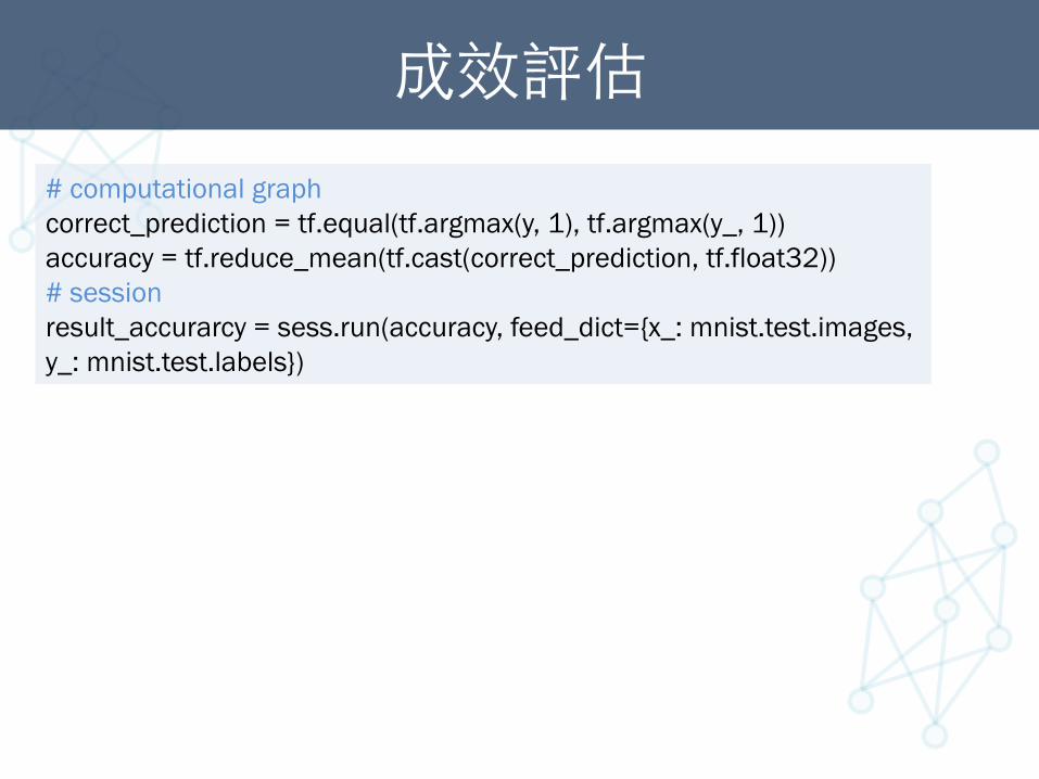
成效評估 # computational graph correct_prediction = tf.equal(tf.argmax(y, 1), tf.argmax(y_, 1)) accuracy = tf.reduce_mean(tf.cast(correct_prediction, tf.float32)) # session result_accurarcy = sess.run(accuracy, feed_dict={x_: mnist.test.images, y_: mnist.test.labels})
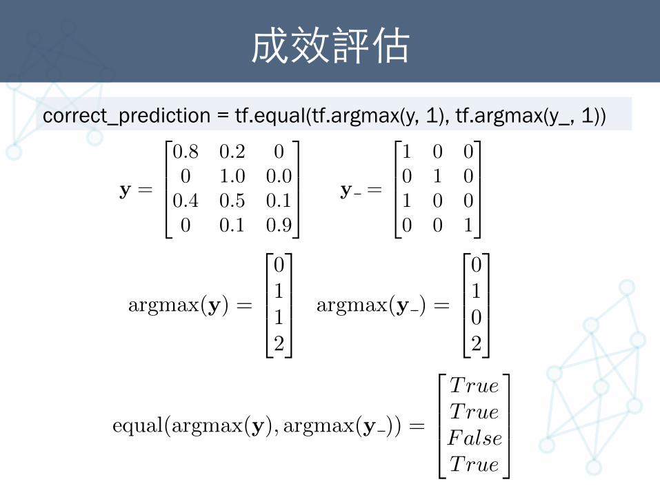
成效評估 correct_prediction = tf.equal(tf.argmax(y, 1), tf.argmax(y_, 1))
y =
2
664
0.8 0.2 00 1.0 0.00.4 0.5 0.10 0.1 0.9
3
775 y =
2
664
1 0 00 1 01 0 00 0 1
3
775
argmax(y) =
2
664
0
1
1
2
3
775 argmax(y ) =
2
664
0
1
0
2
3
775
equal(argmax(y), argmax(y )) =
2
664
TrueTrueFalseTrue
3
775
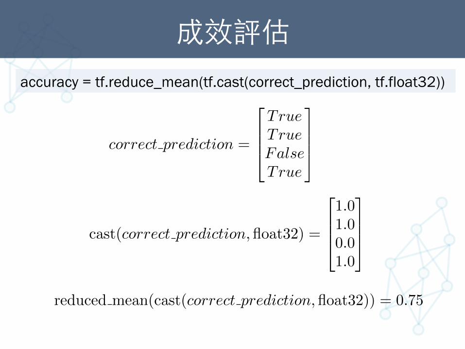
成效評估 accuracy = tf.reduce_mean(tf.cast(correct_prediction, tf.float32))
correct prediction =
2
664
True
True
False
True
3
775
cast(correct prediction, float32) =
2
664
1.0
1.0
0.0
1.0
3
775
reduced mean(cast(correct prediction, float32)) = 0.75
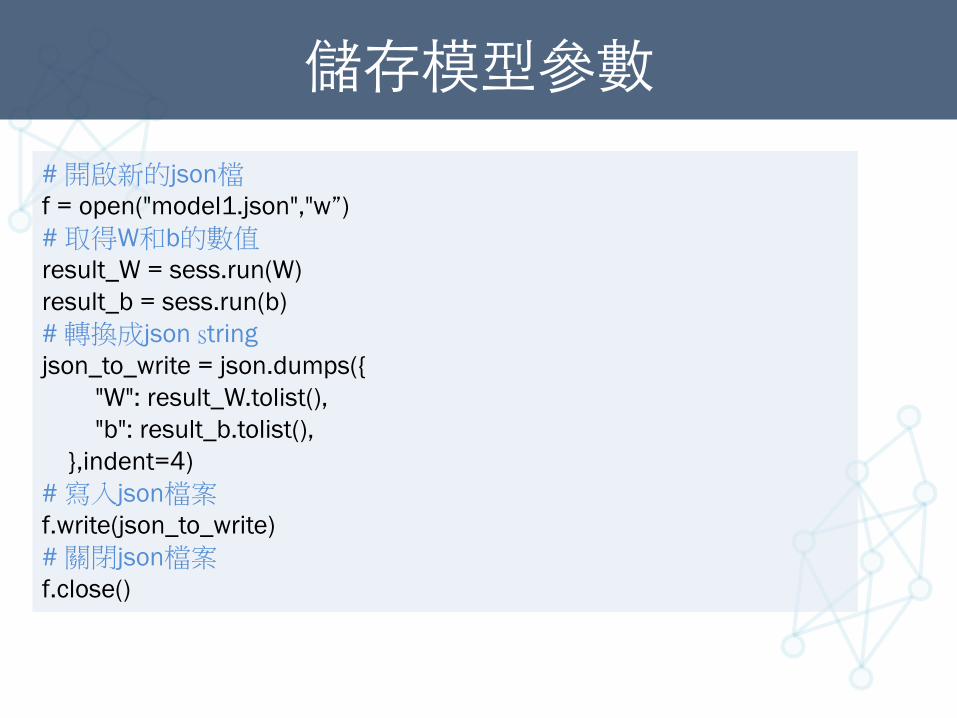
儲存模型參數 # 開啟新的json檔 f = open("model1.json","w”) # 取得W和b的數值 result_W = sess.run(W) result_b = sess.run(b) # 轉換成json string json_to_write = json.dumps({ "W": result_W.tolist(), "b": result_b.tolist(), },indent=4) # 寫入json檔案 f.write(json_to_write) # 關閉json檔案 f.close()
單層感知器模型載⼊入 https://github.com/ckmarkoh/ntc_deeplearning_tensorflow/blob/master/sec1/mnist_load.ipynb
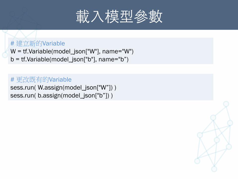
載⼊入模型參數 # 建立新的Variable W = tf.Variable(model_json["W"], name="W") b = tf.Variable(model_json["b"], name="b”)
# 更改既有的Variable sess.run( W.assign(model_json["W”]) ) sess.run( b.assign(model_json["b”]) )
單層感知器Tensorboard https://github.com/ckmarkoh/ntc_deeplearning_tensorflow/blob/master/sec1/mnist_board.ipynb
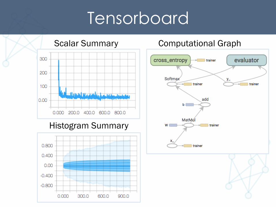
Tensorboard
Histogram Summary
Scalar Summary Computational Graph
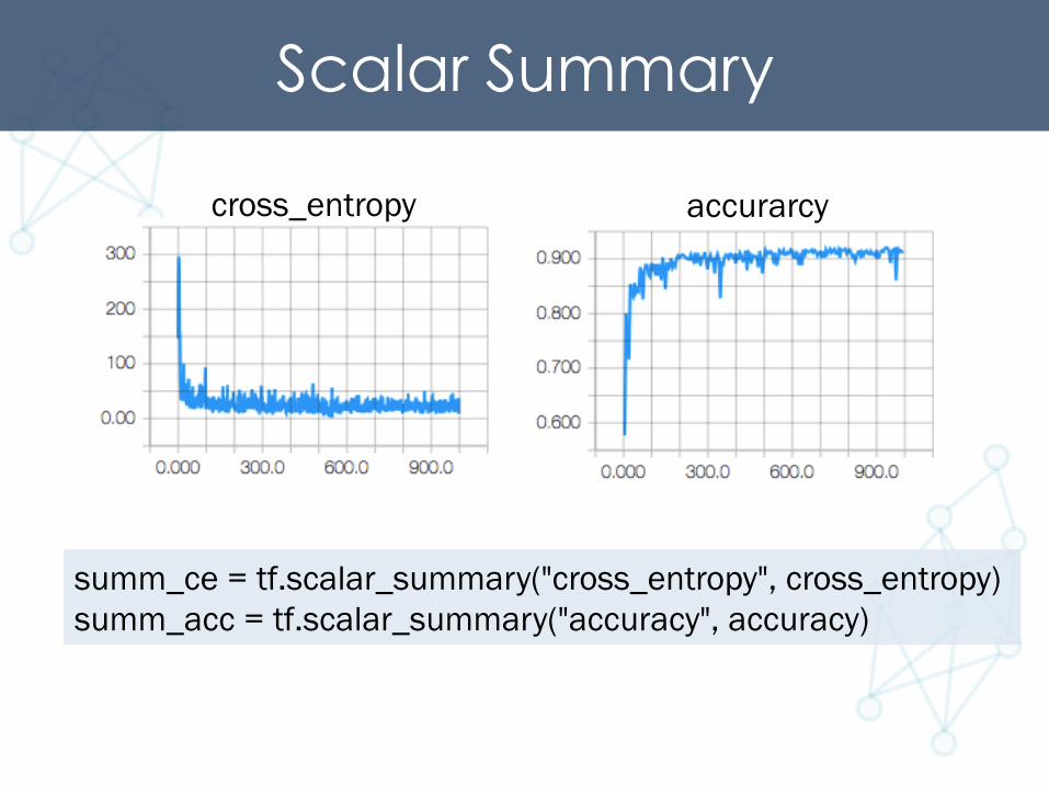
Scalar Summary
summ_ce = tf.scalar_summary("cross_entropy", cross_entropy) summ_acc = tf.scalar_summary("accuracy", accuracy)
cross_entropy accurarcy
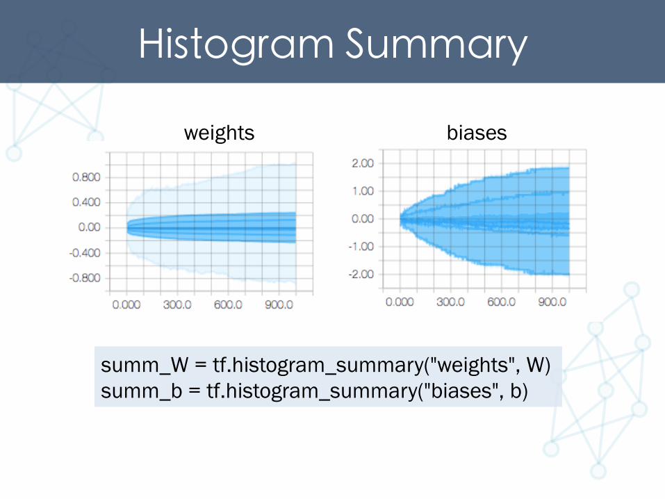
Histogram Summary
summ_W = tf.histogram_summary("weights", W) summ_b = tf.histogram_summary("biases", b)
weights biases
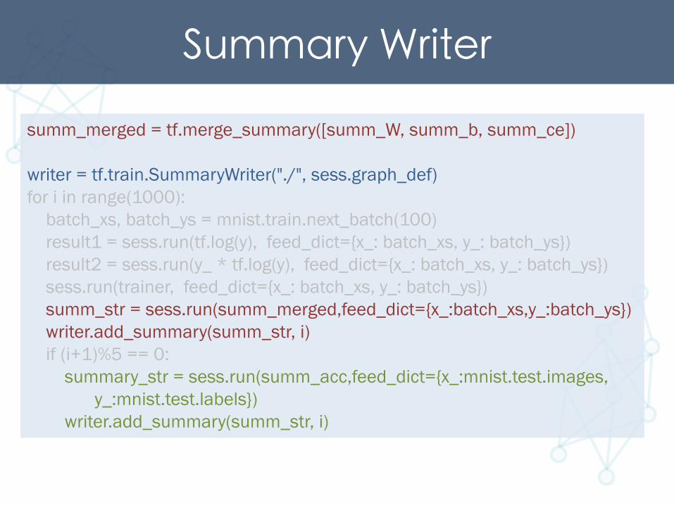
Summary Writer summ_merged = tf.merge_summary([summ_W, summ_b, summ_ce]) writer = tf.train.SummaryWriter("./", sess.graph_def) for i in range(1000): batch_xs, batch_ys = mnist.train.next_batch(100) result1 = sess.run(tf.log(y), feed_dict={x_: batch_xs, y_: batch_ys}) result2 = sess.run(y_ * tf.log(y), feed_dict={x_: batch_xs, y_: batch_ys}) sess.run(trainer, feed_dict={x_: batch_xs, y_: batch_ys}) summ_str = sess.run(summ_merged,feed_dict={x_:batch_xs,y_:batch_ys}) writer.add_summary(summ_str, i) if (i+1)%5 == 0: summary_str = sess.run(summ_acc,feed_dict={x_:mnist.test.images,
y_:mnist.test.labels}) writer.add_summary(summ_str, i)
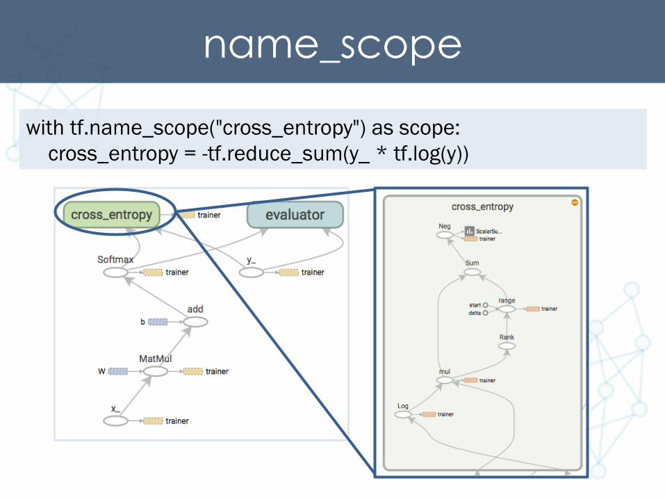
name_scope with tf.name_scope("cross_entropy") as scope: cross_entropy = -tf.reduce_sum(y_ * tf.log(y))

Launch Tensorboard > tensorboard --logdir=./ Starting TensorBoard on port 6006 (You can navigate to http://0.0.0.0:6006)

講師資訊
• Email: ckmarkoh at gmail dot com • Blog: http://cpmarkchang.logdown.com • Github: https://github.com/ckmarkoh
Mark Chang
• Facebook: https://www.facebook.com/ckmarkoh.chang • Slideshare: http://www.slideshare.net/ckmarkohchang • Linkedin:
https://www.linkedin.com/pub/mark-chang/85/25b/847
90