teorÍa cinÉtica de fluidos granulares forzados

TESIS DOCTORAL

TEORIacuteA CINEacuteTICA DE FLUIDOSGRANULARES FORZADOS

AutorMoiseacutes Garciacutea Chamorro

DirectoresVicente Garzoacute PuertosFrancisco Vega Reyes

Departamento de Fiacutesica

2017

University of Extremadura

Doctoral Thesis

Kinetic theory of driven granularfluids

Author

Moises Garcıa

Chamorro

Supervisors

Dr Vicente Garzo

Puertos

Dr Francisco Vega

Reyes

A thesis submitted in fulfilment of the requirements

for the degree of Doctor of Philosophy

in the

Department of Physics

2017

UNIVERSIDAD DE EXTREMADURA

Resumen

Facultad de Ciencias Departmento de Fısica

Doctor en Ciencias

Teorıa cinetica de fluıdos granulares forzados

por Moises Garcıa Chamorro

Los materiales granulares en condiciones de flujo rapido pueden modelarse como

un gas granular esto es un gas compuesto de esferas duras inelasticas que disipan

parte de su energıa cinetica durante colisiones binarias Dada la naturaleza disi-

pativa de las colisiones es necesario inyectar energıa al sistema para compensar

el enfriamiento inelastico y mantener el gas en regimen de fluido rapido Aunque

en experimentos la inyeccion externa de energıa se realiza a traves de paredes

es muy usual encontrar simulaciones por ordenador en las que esta inyeccion se

realiza mediante fuerzas que actuan homogeneamente en todo el sistema A estas

fuerzas se les denomina de forma general termostatos El uso de estos termostatos

ha sido ampliamente utilizado en las ultimas decadas pero su influencia sobre las

propiedades dinamicas de un gas granular no esta aun completamente entendida

En la presente tesis se determinan las propiedades de transporte y reologicas de

sistemas granulares forzados usando dos rutas independientes y complementarias

la primera de ellas analıtica por medio del metodo de Chapman-Enskog solucion

BGK de la ecuacion cinetica y metodo de los momentos de Grad y la segunda

computacional a traves de simulaciones numericas de Monte Carlo

UNIVERSITY OF EXTREMADURA

Abstract

Faculty of Sciences Department of Physics

Doctor of Philosophy

Kinetic theory of driven granular fluids

by Moises Garcıa Chamorro

Granular matter under rapid flow conditions can be modeled as a granular gas

namely a gas of hard spheres dissipating part of their kinetic energy during binary

collisions (inelastic hard spheres IHS) On the other hand given that collisions

are inelastic one has to inject energy into the system to compensate for the inelas-

tic cooling and maintain it in rapid conditions Although in real experiments the

external energy is supplied to the system by the boundaries it is quite usual in

computer simulations to heat the system by the action of an external driving force

or thermostat Despite thermostats have been widely employed in the past their

influence on the dynamic properties of the system (for elastic and granular fluids)

is not yet completely understood In this work we determine the transport prop-

erties of driven granular systems by using two independent and complementary

routes one of them being analytic (Chapman-Enskog method BGK solution and

Gradrsquos moments method) and the other one being computational (Monte Carlo

simulations)

Acknowledgements

Firstly I would like to express my sincere gratitude to my advisors Prof Vicente

Garzo and Prof Francisco Vega Reyes for the continuous support of my PhD

study and related research They offerred me their immense patience motivation

and knowledge Their constant guidance helped me in all the time of research

and writing of this thesis I could not have imagined having a better advisor and

mentor for my PhD study

Besides my advisors I would like to thank my thesis external review commit-

tee Prof Mariano Lopez de Haro and Prof Rodrigo Soto for their insightful

reading and comments and also for the hard question which incented me to widen

my research from various perspectives

My sincere thanks also goes to Prof Emmanuel Trizac who provided me an

opportunity to join their team as intern and who gave access to the laboratory

and research facilities

I thank my department fellows and labmates Andres Santos Juan Jesus Ruiz

Santos Bravo Enrique Abad Miguel Angel Gonzalez Antonio Gordillo and An-

tonio Astillero for the stimulating coffee discussions help and for all the fun we

have had in the last five years

I am grateful to Ministerio de Ciencia en Innovacion for the finantial support

through grant No FIS2010-16587 from the Spanish Government (Spain)

Last but not the least I would like to thank my parents Timoteo and Maxima

and my sister Gema for supporting me spiritually throughout writing this thesis

and my life in general

vii

Contents

Abstract v

Acknowledgements vii

Contents vii

List of Figures xiii

Abbreviations xix

Symbols xxi

1 Introduction to granular gases 1

11 Introduction 1

12 Granular Gases 3

13 Structure of the Thesis 8

2 Kinetic Theory of driven granular gases 13

21 Introduction 13

22 The model for Driven Granular Gases 14

23 The Chapman-Enskog method 19

24 Gradrsquos moment method 22

25 Direct Simulation Monte Carlo method 23

251 Description of DSMC method 24

3 Homogeneous state 27

31 Introduction 27

32 Enskog Kinetic Theory forHomogeneous Driven States 28

33 Analytical solution of the scaled distribution function 32

34 Numerical solutions of the BE equation 35

341 Comparison between theory and simulations 36

3411 Transient regime 36

ix

Contents x

3412 Steady regime 38

35 Summary and Discussion 42

4 Transport properties for driven granular fluids in situations closeto homogeneous steady states 47

41 Introduction 47

42 Small spatial perturbations around the Homogeneous Steady State 48

421 Zeroth-order approximation 49

422 First-order approximation 55

43 Transport coefficients 56

431 Viscosity 56

432 Thermal conductivity 57

433 Cooling rate 58

434 Special limits 59

44 Comparison with computer simulations 61

441 Comparison with stochastic thermostat data 67

45 Linear stability analysis of the hydrodynamic equations 68


5 Navier-Stokes transport coefficients for driven inelastic Maxwellmodels 79

51 Introduction 79

52 Inelastic Maxwell Models 81

53 Homogeneous steady states 83

54 Chapman-Enskog method for states close to homogeneous steadystates 85




551 Transport coefficients under steady state 91

552 Comparison with the steady state transport coefficients forIHS 92


6 Non-Newtonian hydrodynamics for a dilute granular suspensionunder uniform shear flow 101

61 Introduction 101

62 Description of the system 104

621 Boltzmann kinetic equation for granular suspensions 104

622 Steady base state the uniform shear flow 106

623 Characteristic time scales and dimensionless numbers 109

63 Theoretical approaches 113

631 Gradrsquos moment method of the Boltzmann equation 113

632 BGK-type kinetic model of the Boltzmann equation 114

64 Numerical solutions DSMC method 115

Contents xi

65 Results 116

651 Dilute granular suspensions 116

652 Granular suspensions at moderate densities 123


7 Conclusions and Outlooks 131

71 Conclusions 131

72 Outlooks 133

8 Conclusiones y Lıneas Futuras 135

81 Conclusiones 135

82 Lıneas futuras 138

A Expressions for Ai Bi and Ci 141

A1 Expressions for Ai Bi and Ci 141

A2 Approximations I and II 142

B First-order approximation 145

C Kinetic contributions to the transport coefficients 149

D Expressions for choice B 155

E Collisional moments of JIMM[f f ] 157

F First-order contributions to the fluxes for Inelastic Maxwell Mod-els 159

G Transport coefficients for IHS in the steady state 163

H Results from Gradrsquos moment method Rheological properties 165

I Results from the BGK-like kinetic model 169

J Expressions from linear Gradrsquos moments method at moderatedensities 173

Bibliography 177

List of Figures

31 Time evolution for hard disks of the reduced temperature T (t)Ts(a) and the scaled distribution function ϕ(c0) (b) for ξlowast = 0478γlowast = 0014 and α = 09 Three different initial temperatures havebeen considered T (0)Ts = 025(times) 1(middot middot middot ) and 4() Here Ts isthe steady value of the temperature and c0(t) = v0sv0(t) v0s =radic

2Tsm being the steady value of the thermal speedThe symbolscorrespond to the simulation results while the horizontal lines referto the theoretical predictions for Ts and ϕ(c0) The latter has beenobtained by retaining the three first Sonine polynomials (see Eq(347)) and evaluating a2 and a3 with Approximation II Time ismeasured in units of νminus1 (tlowast = tνminus1) 38

32 Plot of the second Sonine coefficient a2 versus the coefficient of resti-tution α for hard disks (a) and hard spheres (b) The symbols referto three different systems with different values of the simulationparameters γlowastsim and ξlowastsim but with the same value of ξlowast (ξlowast = 126for disks and ξlowast = 168 for spheres) The solid and dashed linesare the values obtained for a2 by means of Approximation I andApproximation II respectively 40

33 Plot of the third Sonine coefficient a3 versus the coefficient of resti-tution α for hard disks (a) and hard spheres (b) The symbols referto three different systems with different values of the simulationparameters γlowastsim and ξlowastsim but with the same value of ξlowast (ξlowast = 126for disks and ξlowast = 168 for spheres) The solid and dashed linesare the values obtained for a3 by means of Approximation I andApproximation II respectively 41

34 Plot of the second Sonine coefficient a2 versus the (reduced) noisestrength ξlowast for α = 07 in the case of hard disks (a) and hard spheres(b) The symbols refer to simulation results while the solid anddashed lines are the values obtained for a2 by means of Approx-imation I and Approximation II respectively The vertical linesindicate the threshold values ξlowastth 42

35 Plot of the third Sonine coefficient a3 versus the (reduced) noisestrength ξlowast for α = 07 in the case of hard disks (a) and hardspheres (b) The symbols refer to simulation results while the solidand dashed lines are the values obtained for a3 by means of Approx-imation I and Approximation II respectively The vertical linesindicate the threshold values ξlowastth 43

xiii

List of Figures xiv

36 Plot of the scaled distribution function ϕ(c ξlowast)ϕM(c) in the steadystate for α = 08 The symbols refer to DSMC data obtainedfor three different systems with parameters γlowastsim ξlowastsim = (14 times10minus2 52times 10minus5) (98times 10minus3 18times 10minus5) (7times 10minus3 65times 10minus6) ford = 2 and γlowastsim ξlowastsim = (71 times 10minus3 29 times 10minus6) (5 times 10minus3 98 times10minus7) (36times 10minus3 36times 10minus7) for d = 3 These values yield a com-mon value of ξlowast ξlowast = 1263 for d = 2 and ξlowast = 1688 for d = 3The lines correspond to Eq (347) with expressions for the cumu-lants given by Approximation I (solid lines) and Approximation II(dashed lines) 44

37 Plot of the scaled distribution function ϕ(c ξlowast)ϕM(c) in the steadystate for α = 06 The symbols refer to DSMC data obtainedfor three different systems with parameters γlowastsim ξlowastsim = (14 times10minus2 29times10minus4) (98times10minus3 10minus4) (7times10minus3 36times10minus5) for d = 2and γlowastsim ξlowastsim = (71times10minus3 15times10minus5) (5times10minus3 54times10minus6) (36times10minus3 19 times 10minus6) for d = 3 These values yield a common valueof ξlowast ξlowast = 1263 for d = 2 and ξlowast = 1688 for d = 3 The linescorrespond to Eq (347) with expressions for the cumulants givenby Approximation I (solid lines) and Approximation II (dashed lines) 45

41 Plot of the reduced granular temperature TsTb versus the volumefraction φ for a two-dimensional (d = 2) granular fluid and two dif-ferent values of the coefficient of restitution α = 08 (solid line) andα = 06 (dashed line) The symbols are the Monte Carlo simulationresults (circles for α = 08 and triangles for α = 06) 48

42 Plot of the derivative versus the coefficient of restitution α for thestochastic thermostat ξlowasts = ζlowasts for disks (d = 2) and spheres (d = 3)The solid line is the result given by Eq (422) while the dashed lineis the result obtained by Garcıa de Soria et al [170] 54

43 Plot of the kinematic viscosity ν = ηρ as a function of the volumefraction φ for α = 06 The solid line is the theoretical predic-tion given by Eq (433) while the dashed line is the theoreticalresult obtained by assuming the elastic form of the shear viscosityη Symbols are the simulation results obtained by Gradenigo et al[55] from the static (circles) and dynamical (triangle) correlationsof transversal shear modes 62

44 Plot of the longitudinal viscosity νl as a function of the volumefraction φ for two values of the coefficient of restitution α = 08(panel a) and α = 06 (panel b) The solid lines are the theoreticalpredictions for νl obtained by using Eqs (433) and (435) whilethe dashed lines are the theoretical results obtained by assumingthe elastic forms of the shear viscosity η and the bulk viscosity λSymbols are the simulation results obtained by Gradenigo et al [55]by fitting their numerical data for the dynamical correlations of thelongitudinal modes 63

List of Figures xv

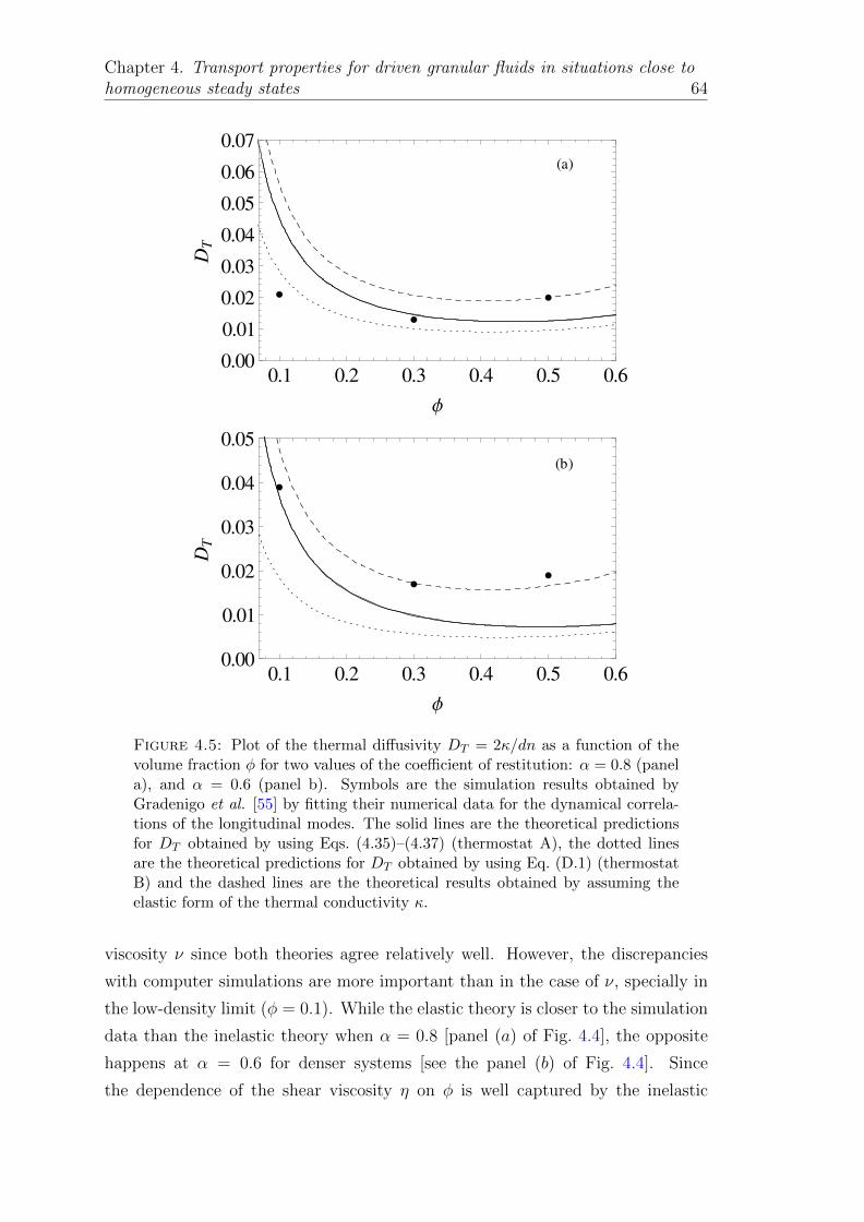
45 Plot of the thermal diffusivity DT = 2κdn as a function of thevolume fraction φ for two values of the coefficient of restitutionα = 08 (panel a) and α = 06 (panel b) Symbols are the sim-ulation results obtained by Gradenigo et al [55] by fitting theirnumerical data for the dynamical correlations of the longitudinalmodes The solid lines are the theoretical predictions for DT ob-tained by using Eqs (435)ndash(437) (thermostat A) the dotted linesare the theoretical predictions for DT obtained by using Eq (D1)(thermostat B) and the dashed lines are the theoretical results ob-tained by assuming the elastic form of the thermal conductivity κ 64

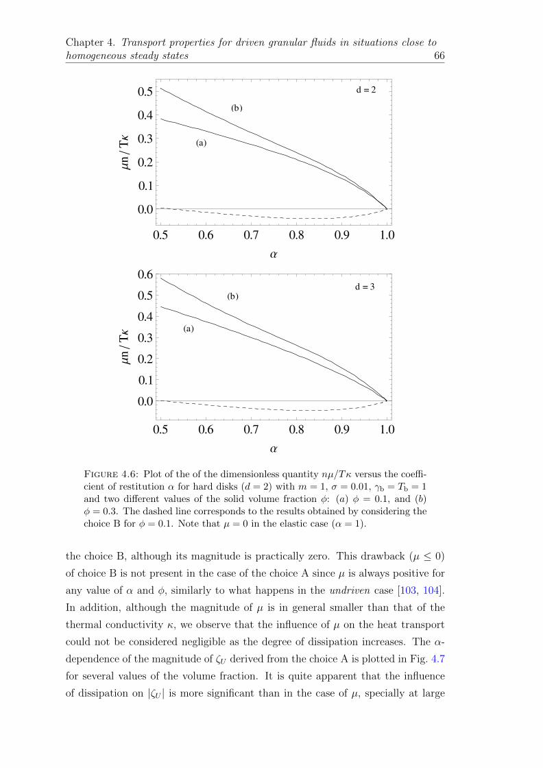
46 Plot of the of the dimensionless quantity nmicroTκ versus the coeffi-cient of restitution α for hard disks (d = 2) with m = 1 σ = 001γb = Tb = 1 and two different values of the solid volume fraction φ(a) φ = 01 and (b) φ = 03 The dashed line corresponds to theresults obtained by considering the choice B for φ = 01 Note thatmicro = 0 in the elastic case (α = 1) 66

47 Plot of the magnitude of the first-order contribution ζU to the cool-ing rate versus the coefficient of restitution α with m = 1 σ = 001γb = Tb = 1 and three different values of the solid volume fractionφ (a) φ = 01 (b) φ = 03 and (c) φ = 05 Note that ζU = 0 inthe elastic case (α = 1) 67

48 Plot of the thermal diffusivity DT as a function of the volume frac-tion φ for α = 09 and α = 08 Solid and dashed lines are thetheoretical predictions for DT obtained by using Eqs (437)ndash(439)(thermostat A) and Eq (D1) (thermostat B) respectively whereasdotted line correspond to the preditions for the undriven gas Cir-cles and triangles are simulation data 69

49 Plot of the dispersion relations for disks (d = 2) and spheres (d = 3)with σ = 001 φ = 02 and α = 08 Line (a) corresponds tothe d minus 1 degenerate transversal modes while (b) and (c) are theremaining longitudinal modes Only the real parts of the eigenvaluesof the matrix M is plotted 73

51 The steady fourth-cumulant a2s as a function of the coefficient ofrestitution for a three-dimensional system (d = 3) for ξlowasts = 062The solid and dashed lines are the results obtained for IMM andIHS respectively The symbols (circles for IMM and squares forIHS) refer to the Monte Carlo simulation results 84

52 Plot of the derivative ∆ equiv(parta2partξlowast

)sversus the coefficient of restitution

α for the stochastic thermostat (ξlowasts = ζlowasts ) for disks (d = 2) andspheres (d = 3) The solid lines are the results given by Eq (552)for q = 1

2while the dashed lines are the results obtained for IHS 93

List of Figures xvi

53 Plot of the reduced shear viscosity ηlowasts ηlowasts0 as a function of the co-

efficient of restitution α for β = 12

in the case of a two- and three-dimensional system of IMM with q = 1

2(solid lines) and IHS (dashed

lines) The value of the (reduced) noise strength is ξlowasts = 1 94

54 The same as in Fig 53 for the reduced thermal conductivity κlowastsκlowasts0 95

55 The same as in Fig 53 for the reduced coefficient microlowasts = nmicrosκ0T 96

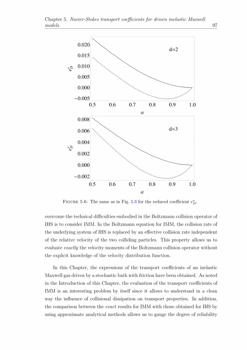
56 The same as in Fig 53 for the reduced coefficient elowastD 97

61 St(α γlowast) surface for a dilute suspension of granular particles Thecontours for St = 6 10 have been marked in the St = 0 plane 110

62 Scheme of the flow regimes as they result from the relation (611)between the (reduced) shear rate alowast the (reduced) friction coeffi-cient γlowast and the Stokes number St for a dilute granular suspensionunder USF Blue (symbols and lines) stands for the case α = 05and black (symbols and lines) stands for the case α = 09 Thesolid lines correspond to the results derived from Gradrsquos momentmethod while the dashed lines refer to the NS predictions Panel(a) Reduced shear rate alowast vs γlowast Panel (b) Stokes number St vsγlowast In this panel the three regions commented in the text have beenmarked a high Knudsen number region to the right of the panel (inpale red) a lowmoderate Knudsen number region (in white) andfinally in the lower part of the panel the forbidden small St region(green) may be found 111

63 Dependence of the (reduced) elements of the pressure tensor P lowastxx(panel (a)) and P lowastxy (panel (b)) on the Stokes number St for severalvalues of the coefficient of restitution α α = 1 (black) α = 07(blue) and α = 05 (red) The solid lines are the theoretical resultsobtained from nonlinear Gradrsquos solution while the symbols refer tothe results obtained from DSMC We have marked as vertical dottedlines the minimum allowed value for the Stokes number St 117

64 Dependence of the (reduced) diagonal elements of the pressure ten-sor P lowastyy (black lines and squares) and P lowastzz (blue lines and triangles)on the Stokes number St for several values of the coefficient of resti-tution α α = 1 (a) α = 07 (b) and α = 05 (c) The solid linesare the theoretical results obtained from nonlinear Gradrsquos solutionwhile the symbols refer to the results obtained from DSMC Asin Fig 63 we have marked as vertical dotted lines the minimumallowed value of the Stokes number St for each value of α 118

65 Plot of the (reduced) nonzero elements of the pressure tensor P lowastxx(panel a) P lowastxy (panel b) P lowastyy and P lowastzz (panel c) as functions of thecoefficient of restitution α for γlowast = 05 The solid and dotted linescorrespond to the results obtained from nonlinear and linear Gradrsquossolution respectively Symbols refer to DSMC In the panel (c) theblue solid line and triangles are for the element P lowastzz while the blacksolid line and squares are for the element P lowastyy Note that linearGradrsquos solution (dotted line) yields P lowastyy = P lowastzz 119

List of Figures xvii

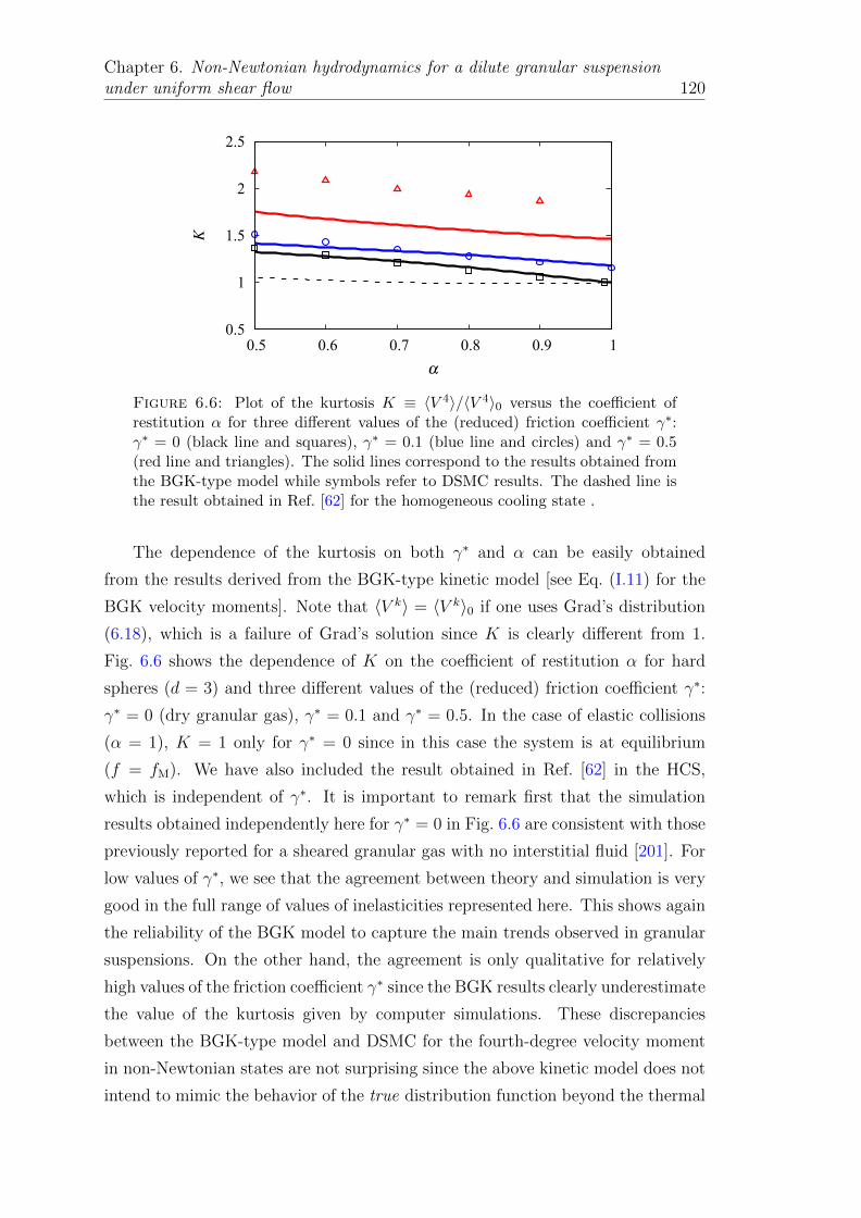
66 Plot of the kurtosis K equiv 〈V 4〉〈V 4〉0 versus the coefficient of restitu-tion α for three different values of the (reduced) friction coefficientγlowast γlowast = 0 (black line and squares) γlowast = 01 (blue line and circles)and γlowast = 05 (red line and triangles) The solid lines correspond tothe results obtained from the BGK-type model while symbols referto DSMC results The dashed line is the result obtained in Ref [62]for the homogeneous cooling state 120

67 Logarithmic plots of the marginal distribution function ϕ(+)x (cx) as

defined in Eq (I15) Two cases are represented here (a) α = 09γlowast = 01 and (b) α = 05 γlowast = 01 The black and blue solidlines are the theoretical results derived from the BGK model andthe ME formalism respectively while the symbols represent thesimulation results The red dotted lines are the (local) equilibriumdistributions 121

68 Logarithmic plots of the marginal distribution function ϕ(+)y (cy) as


69 Plot of the reduced steady shear viscosity micros and the square rootof the steady granular temperature θ12 as a function of StRdiss

in the case of hard spheres (d = 3) with α = 1 and φ = 001The solid black lines are the Gradrsquos solution (including nonlinearcontributions) to the Boltzmann equation the dashed (blue) linescorrespond to the BGK results (which coincide with those obtainedfrom the linear Gradrsquos solution) and the dotted (red) lines refer tothe results obtained from the Enskog equation by applying (linear)Gradrsquos method The circles are the simulation results obtained bySangani et al [92] while the triangles correspond to the DSMCcarried out in this work The green solid lines are the predictionsobtained from the NS hydrodynamic equations derived in Ref [62] 126

610 Plot of the normal stress differences P lowastxx minus P lowastyy and P lowastxx minus P lowastzz as afunction of StRdiss in the case of hard spheres (d = 3) with α = 1and φ = 001 The solid lines are the Gradrsquos solution (includingnonlinear contributions) to the Boltzmann equation for P lowastxx minus P lowastyy(black line) and P lowastxx minus P lowastzz (violet line) the dashed (blue) line cor-responds to the BGK results (which coincide with those obtainedfrom the linear Gradrsquos solution) and the dotted (red) line refers tothe results obtained from the Enskog equation by applying (linear)Gradrsquos method The black and empty circles are the simulationresults obtained by Sangani et al [92] for P lowastxxminus P lowastyy and P lowastxxminus P lowastzzrespectively 127

List of Figures xviii

611 Plot of the square root of the steady granular temperature θ12 as afunction of StRdiss in the case of hard spheres (d = 3) for φ = 001Two different values of the coefficient of restitution have been con-sidered α = 07 (a) α = 05 (b) The solid line is the Gradrsquos solu-tion (including nonlinear contributions) to the Boltzmann equationthe dashed (blue) line corresponds to the BGK results (which coin-cide with those obtained from the linear Gradrsquos solution) and thedotted (red) line refers to the results obtained by Sangani et al[92] from the Enskog equation by applying (linear) Gradrsquos methodThe black circles and triangles are the simulation results obtainedhere by means of the DSMC method for α = 07 and α = 05respectively while the empty triangles are the results obtained inRef [92] 128

Abbreviations

BGK Bhatnagar-Gross-Krook

CE Chapman-Enskog (approach)

DSMC Direct Simulation of Monte Carlo (method)

EHS Elastic Hard Spheres (model)

HCS Homogeneous Cooling State

IHS Inelastic Hard Spheres (model)

IMM Inelastic Maxwell Model

MD Molecular Dynamics (method)

ME Maximum Entropy (formalism)

USF Uniform Shear Flow

NS Navier-Stokes

xix

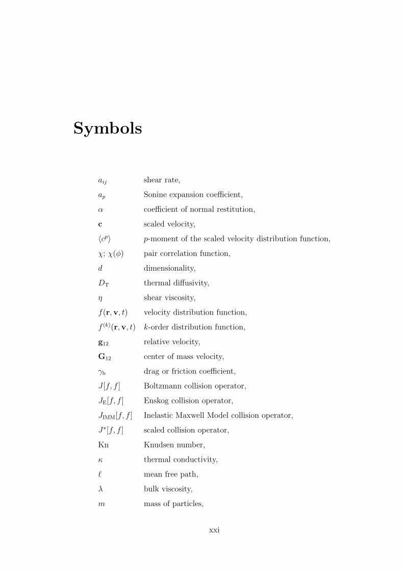
Symbols

aij shear rate

ap Sonine expansion coefficient

α coefficient of normal restitution

c scaled velocity

〈cp〉 p-moment of the scaled velocity distribution function

χ χ(φ) pair correlation function

d dimensionality

DT thermal diffusivity

η shear viscosity

f(rv t) velocity distribution function

f (k)(rv t) k-order distribution function

g12 relative velocity

G12 center of mass velocity

γb drag or friction coefficient

J [f f ] Boltzmann collision operator

JE[f f ] Enskog collision operator

JIMM[f f ] Inelastic Maxwell Model collision operator

Jlowast[f f ] scaled collision operator

Kn Knudsen number

κ thermal conductivity

` mean free path

λ bulk viscosity

m mass of particles

xxi

Symbols xxii

micro diffusive heat conductivity or Dufour-like coefficient

n number density

ν0 collision frequency

Ωd total solid angle in d-dimensions

Pij pressure tensor

Πij traceless pressure tensor

φ solid volume fraction

ϕ(c) scaled velocity distribution function

ρ mass density

T granular temperature

Θ(x) Heaviside step function

σ diameter of particles

σ unit vector joining the centers of colliding particles

U mean flow velocity of solid particles

Ug mean flow velocity of interstitial gas

V peculiar velocity

v0 thermal velocity

ξ2b noise intensity

Dedicated to my parents and sister who always believedin me even when I didnrsquot

xxiii

Chapter 1

Introduction to granular gases

11 Introduction

Granular matter is a vast and diverse family of materials with the common prop-

erty of being composed of a large number of macroscopic grains with very different

shapes and range of sizes [1] This kind of material is quite commonplace in Na-

ture and industry in examples like cereals salt sand etc Their study is of great

interest in a wide variety of the industry and technology sectors as well as in dif-

ferent fields of fundamental and applied science such as biophysics astrophysics

fluid mechanics statistical physics and even in optics applications

The knowledge of physical properties of granular matter has also great prac-

tical importance in Engineering for the design of many industrial processes such

as conveying handling and storage This is important because it might prevent

malfunctions of the devices due to phenomena of obstructions irreversible stuck

of grains and potentially dramatic events such as the collapse of a silo It is also

usual to deal with processes of separating or mixing several substances in the form

of powder for the manufacturing of pharmaceutical or chemical products[2]

Some authors estimate that nowadays granular matter is involved in more

than 50 of trade in the world [3] Many of the products we daily use have been

made using granular matter in a stage of their fabrication process In fact granular

media are the second most used type of material in industry after water Rough

estimates of the losses suffered in the world economy due to granular ignorance

amount to billions of dollars a year [1]

1

Chapter 1 Introduction to granular gases 2

But not only in Earth one can find this kind of material Out of our planet

granular matter also abounds in space in the form of dust and grains This is il-

lustrated for instance by Martian dunes or astronomic-range features as planetary

rings asteroids comets clouds (as the Kuiperrsquos Belt and the Oortrsquos Cloud) and

interstellar dust that reach vital importance for the proper functioning of commu-

nication satellites probes and man ships such as the International Space Station

[4 5 6 7]

On the other hand although in nature one can find granular systems in vacuum

(as for instance the previous mentioned interstellar dust) in most cases of interest

granular particles are immersed in a fluid (air water etc) This kind of mixtures

(granular suspensions) is widely used in many industrial processes for instance

in civil engineering works with concretes asphalt bitumen or in the chemical

industry in fuel or catalysts deployed in the form of grain to maximize the active

surfaces

Another interesting problem where granular theories are useful is the diffusion

of fluids through densely packed cobblestone and rocks that is vital for the indus-

try of natural combustibles and subterranean water findingThe comprehension

of the coupling between fluid and solid phase is essential in geological problems

as soil stability and water controls surface modelling by soil erosion sand dunes

movement and the dangerous ripples formation in the sand under shallow sea wa-

ter Furthermore understanding of the dynamics of many natural disasters such

as avalanches landslides mud flows pyroclastic flows etc can be achieved by

means of models of granular media [8] In particular an important target of the

research in granular matter concerns the description and prediction of natural haz-

ards that the above events suppose to the human activities in order to avoid or

minimize their impact on lives and economy around the world [9]

Apart from their industrial and geophysical applications there exist many

important scientific reasons to study the laws underlying the behaviour of granular

materials On the other hand despite its practical importance our understanding

of granular media remains still incomplete No theoretical framework is available

to describe the different phenomena observed in nature for granular flows

It is well-known that granular media can behave like a solid liquid or a gas [10]

Grains can create static structures sustaining great stresses but they can also flow


as liquids or even gases when strongly excited In addition the three states can co-

exist in a single system In spite of this it is not so easy to accept that such flow can

be described by hydrodynamic equations [11 12] Notwithstanding when the sys-

tem is externally driven (rapid flow regime) fluidized granular media may exhibit

most of the known hydrodynamic flows and instabilities such as Taylor-Couette

[13] and Couette-Fourier [14] flows Benard convection [15] etc Furthermore

they may present a complex rheology exhibiting different non-Newtonian features

as nonzero anisotropic normal stresses differences and non-linear relation between

the shear stress and the shear rate much like in other non-Newtonian materials

The normal stress in these fluids is often anisotropic like in other non-Newtonian

materials In addition they show features that do have not their counterpart in

ordinary fluids For instance in vertically vibrated shallow layers of grains stable

geyser-like excitations called oscillons can be observed [16]

This intriguing behaviour intermediate between solid and fluid is a basic char-

acteristic of granular matter Above certain density threshold the system becomes

a compact solid because of the dissipating character of grain interactions but if

the system is externaly excited or its density is decreased then it can flow

For all these reasons in the last years a vast bibliography on granular dynamics

has been reported [17 18]

12 Granular Gases

Generally we may differentiate the high and low density regimes in granular mat-

ter The latter regime is essentially characterized by binary particle collisions

whereas the former presents multiparticle contacts As a consequence the theo-

retical modeling and mathematical treatment to obtain their physical properties

are quite different in each regime [18] In this work we will focus on the binary col-

lision regime where the system is usually called a granular gas [19] whose physical

realization can be observed in rings of planets small planets suspended particles

in fluidized beds aerosols rapid granular flows etc [20]

One of the fundamental properties of the grains in granular matter is the

inelastic character of their collisions When two particles collide part of their

kinetic energy is irreversibly transformed into internal degrees of freedom (tem-

perature rising of particles plastic deformations etc) This provokes a persistent


loss of mechanical energy in the whole system Dissipative interactions between

particles in unforced granular gases is the reason for which these systems are inher-

ently out of equilibrium Granular gases also reveal self-organized spatio-temporal

structures and instabilities When a granular gas has no energy input then it

become unstable to density perturbations and if they freely evolve they will even-

tually collapse by a mechanism of clustering instabilities (which is increasingly

stronger with increasing inelasticity) that will destroy the homogeneity of the sys-

tem [21 22 23 24 25] This tendency to collapse into clusters occurs even for

initially prepared homogeneous mass distributions [24 26 27] The clustering

instability can be easily understood from a qualitative argument Fluctuations

of density in granular gases generate relatively denser domains where the rate of

collisions (proportional to the number density) is higher than in dilute domains

and hence the kinetic energy loss due to inelasticity increases in these regions

As a result the grains tend to move from dilute into dense domains driven by

the granular pressure difference between them thereby further increasing the den-

sity of the latter and giving rise to bigger and denser clusters This mechanism

allows for the growing of the clusters which may further coagulate by coarsen-

ing with other into larger clusters [18] or collide thereby destroying each other

[24 28 29 30] The critical length scale for the onset of instability can be de-

termined via stability analysis of the linearized Navier-Stokes (NS) hydrodynamic

equations [31 32 33 34 35 36 37 38 39]

In order to maintain the system in rapid flow conditions it is neccesary to com-

pensate the loss of energy due to the inelastic dissipation with the introduction of

external non-conservative forces acting over the whole system This is commonly

done either by driving through the boundaries (eg shearing the system or vibrat-

ing its walls [25 40 41]) or alternatively by bulk driving (as in air-fluidized beds

[42]) gravity (as in a chute) or other techniques On the other hand this way of

supplying energy causes in most of the cases strong spatial gradients in the system

To avoid the difficulties associated with non-homogeneous states it is quite usual

in computer simulations to homogeneously heat the system by the action of an

external driving force [43 44 45 46 47 48 49 50 51 52 53 54 55] Borrowing

a terminology often used in nonequilibrium molecular dynamics of ordinary fluids

[56] this type of external forces are usually called thermostats Nevertheless in

spite of its practical importance the effect of the external driving force on the

dynamical properties of the system (such as the transport coefficients) is still not

completely understood [57 58 59] In particular recent computer simulations


[54 55] have obtained some transport coefficients by measuring the static and

dynamical structure factors for shear and longitudinal modes in a driven granular

fluid Given that the expressions for the transport coefficients were not known in

this driven problem the simulation data were compared with their corresponding

elastic system Thus it would be desirable to provide simulators with the appro-

priate theoretical tools to work when studying problems in granular fluids driven

by thermostats

When externally excited a granular system can become sufficiently fluidized

so that the grain interactions are mostly nearly-instantaneous binary collisions and

a steady non-equilibrium state is achieved [18] In this regime each grain moves

freely and independently instead of moving joined in clusters Hence the velocity

of each particle may be decomposed into a sum of the mean or bulk velocity of

the whole system and an apparently random component to describe the motion

of the particle relative to the mean flux usually named peculiar velocity Such

random motion resembles the thermal motion of atoms or molecules in ordinary

gases where the collision time is much smaller than the mean free time between

collisions This analogy between granular and ordinary gases allows one to manage

with a kinetic-theory picture of such systems In that context the mean-square

value of the random velocites is commonly referred to as the granular temperature

This term first coined by Ogawa [60] has nothing to do with the usual thermal

temperature which plays no role in the dynamics of granular flows despite such

name

Under these conditions kinetic theory together with numerical simulations

are the best tools to describe the behaviour and provide constitutive equations

for rapid and diluted granular flows which gives insight into the physical origin

of the transport properties The analogy between granular and ordinary gases

was first introduced by Maxwell in 1859 to describe Saturnrsquos planetary rings [61]

and constitutes one of the most remarkable applications of the kinetic theory of

granular media Thus from the point of view of kinetic theory the study of

granular gases is an interesting and fundamental challenge since it involves the

generalization of classical kinetic equations (such as the Boltzmann Enskog or

Boltzmann-Lorentz equations for instance) to dissipative dynamics

On the other hand driven granular gases can be seen as a prototype model

of a suspension of solid grains inmersed in a fluid in the dilute limit [62] In

those cases the stress due to the grains exceeds that due to the fluid (the ratio of


the two is known as the Bagnold number) so that the effects of the fluid can be

ignored [63] This condition is accomplished for example in aerosols or suspensions

in wich the gravity is balanced with bouyancy [64 65 66] In these systems the

influence of the interstitial fluid on the dynamic properties of the solid phase

is neglected in most theoretical and computational works On the other hand

the effects of the interstitial fluid turns out to be significant for a wide range of

practical applications and physical phenomena like for instance species segregation

[67 68 69 70 71 72 73 74 75 76] or in biophysics where active matter may

be considered as a driven granular suspension [77] For this reason the study of

gas-solid flows has atracted the attention of engineering and physicist commuities

in the last few years [78]

The description of gas-solid suspensions whose dynamics is very complex is a

long-standing branch of classical fluid mechanics [79] For instance particles sus-

pended in a fluid feel a lubrication force transmitted by the surrounding fluid but

originated by the presence of another nearby particle It is known that this kind of

interaction (usually called hydrodynamic interaction) depends also on the global

configuration of the set of grains [80] giving rise to tensor-rank force equations

The modeling of these lubrication forces is rather involved and several approaches

can be used For this reason there is a large bibliography that extends for decades

and that is devoted to the study of this kind of interactions (Stokesian or Stokes

dynamics) [80 81 82]

Nevertheless in the dilute suspension limit these hydrodynamic interactions

become less relevant [79 80] and only the isolated body resistance is retained

usually in the form of a simple drag force On the other hand due to the inher-

ent complexity of the interaction between the interstitial fluid and the granular

particles early kinetic theory studies have neglected in most cases the effect of in-

elasticity in suspended particle collisions [83 84 85 86 87] This kind of approach

is not entirely accurate since of course in most real cases the sizes of suspended

particles are big enough to render particle collisions inelastic (bigger than 1 microm

otherwise particles may be considered as colloids for which collisions are elas-

tic [82 88]) Inelasticity in the collisions can play a major role in the dynamics

of granular (as opposed to colloidal) suspensions specially in the dilute limit at

high Stokes number where grain-grain collisions effects dominate over many par-

ticle hydrodynamic interactions [89] However only more recent works have dealt


with inelastic collisions in the case of dilute [90 91] and moderately dense [92]

suspensions

Despite the apparent similarity between granular and molecular gases there

are however fundamental differences to take into account The first one is related

with the size of the grains in a granular gas Due to the macroscopic dimensions

of the granular particles the typical number of them in laboratory conditions

is much smaller than Avogadrorsquos number and hence the fluctuations of their

hydrodynamic fields are much bigger than in molecular gases [11] However their

number is sufficiently large to admit a statistical description

Granular gases present nevertheless a deeper difference with molecular gases

This difference comes from the inelastic character of collisions which gives rise

to a loss of kinetic energy Thus in order to keep the granular gas in rapid flow

conditions energy must be externally injected into the system to compensate for

the energy dissipated by collisions Therefore granular matter can be considered

as a good example of a system that inherently is a non-equilibrium state

Apart from the collisional cooling there is another fundamental open question

in granular gases the posible lack of separation between microscopic and macro-

scopic length or time scales To apply a continuum hydrodynamic approach it is

necessary that there exists a clear separation between macroscopic and microscopic

scales that is spatial variations of hydrodynamic fields must occur on a length

scale larger than the mean free path of the gas molecules Correspondingly the

typical macroscopic time scale should be larger than the mean free time between

two collisions

However several authors claim that the above scale separation does not exist

for finite dissipation [11 93 94 95 96 97] and the granular hydrodynamic descrip-

tion only applies in the quasi-elastic limit The reason for this concern resides in

the fact that the inverse of the cooling rate (which measures the rate of energy loss

due to collisional dissipation) introduces a new time scale not present for elastic

collisions The variation of the (granular) temperature T over this new time scale

is faster than over the usual hydrodynamic time scale and hence as inelasticity

increases it could be possible that T were not considered a slow variable as in the

usual hydrodynamic description

Despite the above difficulties in recent years it has been proved that it is

possible to apply a hydrodynamic description for the study of granular gases The


main condition for a flow to be considered as a candidate for a hydrodynamic

description is a state of continual collisions This implies that all particles within

each small cell are moving randomly relative to the mean flow velocity of the cell

[98]

Nevertheless the ranges of interest of the physics of granular gases fall fre-

quently beyond Newtonian hydrodynamics since the strength of the spatial gradi-

ents is large in most situations of practical interest (for example in steady states)

This is essentially due to the balance between viscous heating and collisional cool-

ing and usually moderately large spatial gradients can appear [18 99 100] As

said before in these steady states a hydrodynamic description is still valid but

with complex constitutive equations [101 102]

13 Structure of the Thesis

We have organized this thesis as follows

In Chapter 2 we present the details of the model for driven granular gases

previously explained as a paradigm of dilute gas-solid suspensions In addition

we display the general mathematical and numerical tools to be employed in the

present work

Homogeneous steady states of a driven granular fluid are analyzed in Chapter

3 After a transient regime the gas reaches a steady state characterized by a scaled

distribution function ϕ that does not only depend on the dimensionless velocity

c equiv vv0 (v0 being the thermal velocity) but also on the dimensionless driving

force parameters characterizing the external driving forces The dependence of ϕ

and its first relevant velocity moments a2 and a3 (which measure non-Gaussian

properties of ϕ) on both the coefficient of restitution α and the driving parameters

is widely investigated by means of the Direct Simulation Monte Carlo (DSMC)

method In addition approximate forms for a2 and a3 are also derived from an

expansion of ϕ in Sonine polynomials The theoretical expressions of the above

Sonine coefficients agree well with simulation data even for quite small values of

α Moreover the third order expansion of the distribution function makes a signif-

icant accuracy improvement for larger velocities and inelasticities over theoretical

predictions made by considering only the second order expansion Results also


show that the non-Gaussian corrections to the distribution function ϕ are smaller

than those observed for undriven granular gases

The aim of Chapter 4 is to determine the NS transport coefficients of a dense

driven granular gas of inelastic hard spheres in the framework of the Enskog ki-

netic equation Like in the undriven case [103 104] the transport coefficients

are obtained by solving the Enskog equation by means of the Chapman-Enskog

(CE) expansion [105] around a certain reference state f (0) (zeroth-order approxi-

mation) While in the undriven case the distribution f (0) is chosen to be the local

version of the Homogeneous Cooling State (HCS) there is some flexibility in the

choice of f (0) for a driven gas For simplicity one possibility is to take a local

thermostat such that the distribution f (0) is still stationary at any point of the

system This was the choice assumed in previous works [106 107] to compute the

transport coefficients of a heated granular gas On the other hand for general

small deviations from the steady reference state the zeroth-order distribution f (0)

is not in general a stationary distribution since the collisional cooling cannot be

compensated locally by the heat injected by the driving force This fact introduces

additional difficulties not present in previous studies [106 107] In this Chapter

we will adopt this point of view and will consider this kind of thermostat that

seems to be closer to the one used in computer simulations

The determination of the transport coefficients involves like in the undriven

case [31 108] the evaluation of certain collision integrals that cannot be exactly

computed due to the complex mathematical structure of the (linearized) Enskog

collision operator for Inelastic Hard Spheres (IHS) Thus in order to obtain explicit

expressions for the above coefficients one has to consider additional approxima-

tions In Chapter 5 we propose a possible way of circumventing these technical

difficulties inherent to IHS by considering instead the so-called Inelastic Maxwell

Models (IMM) for dilute granular gases As for ordinary gases the collision rate for

these models is independent of the relative velocity of the two colliding particles

In the case of elastic collisions (conventional molecular gases) Maxwell models are

characterized by a repulsive potential that (in three dimensions) is proportional

to the inverse fourth power of distance between particles On the other hand for

inelastic collisions Maxwell models can be introduced in the framework of the

Boltzmann equation at the level of the cross section without any reference to a

specific interaction potential [109] In addition apart from its academic interest

it is worthwhile remarking that experiments [110] for magnetic grains with dipolar


interactions are well described by IMM Therefore the motivation of the Chapter

is twofold On the one hand the knowledge of the first collisional moments for

IMM allows one to re-examine the problem studied in the previous Chapter in the

context of the (inelastic) Boltzmann equation and without taking any additional

and sometimes uncontrolled approximations On the other hand the comparison

between the results obtained from IMM with those derived from IHS [111 112] can

be used again as a test to assess the reliability of IMM as a prototype model for

characterizing real granular flows Previous comparisons have shown a mild quali-

tative agreement in the freely cooling case [113 114] while the agreement between

IMM and IHS significantly increases for low order velocity moments in the case of

driven states (for instance the simple shear flow problem) [18 115 116] The main

advantage of using IMM instead of IHS is that a velocity moment of order k of the

Boltzmann collision operator only involves moments of order less than or equal to

k This allows to evaluate the Boltzmann collision moments without the explicit

knowledge of the distribution function [117] This property opens up the search of

exact solutions to the Boltzmann equation and justifies the interest of physicists

and mathematicians in IMM in the last few years [118 119 120 121 122 123 124

125 126 127 128 129 130 131 132 133 134 135 136 137 138 139 140 141]

Thus in this Chapter we determine in the steady state the exact forms of the

shear viscosity η the thermal conductivity κ and the transport coefficient micro (that

relates the heat flux with the density gradient) as a function of the coefficient of

restitution α and the thermostat forces As for IHS [111] the expressions of η κ

and micro are obtained by solving the Boltzmann equation for IMM up to first order

in the spatial gradients by means of the CE expansion [105]

In Chapter 6 we study a steady laminar shear flow with null heat flux (usually

called uniform shear flow) in a gas-solid suspension at low density The solid

particles are modeled as a gas of smooth hard spheres with inelastic collisions

while the influence of the surrounding interstitial fluid on the dynamics of grains is

modeled by means of a volume drag force in the context of a rheological model for

suspensions The model is solved by means of three different but complementary

routes two of them being theoretical (Gradrsquos moment method applied to the

corresponding Boltzmann equation [142] and an exact solution of a kinetic model

adapted to granular suspensions [143]) and the other being computational (Monte

Carlo simulations of the Boltzmann equation [144]) Unlike in previous studies on

granular sheared suspensions [87 92] the collisional moment associated with the

momentum transfer is determined in Gradrsquos solution by including all the quadratic


terms in the stress tensor This theoretical enhancement allows us for the detection

and evaluation of the normal stress differences in the plane normal to the laminar

flow In addition the exact solution of the kinetic model gives the explicit form of

the velocity moments of the velocity distribution function Comparison between

our theoretical and numerical results shows in general a good agreement for the

non-Newtonian rheological properties the kurtosis (fourth velocity moment of

the distribution function) and the velocity distribution of the kinetic model for

quite strong inelasticity and not too large values of the (scaled) friction coefficient

characterizing the viscous drag force This shows the accuracy of our analytical

results that allows us to describe in detail the flow dynamics of the granular sheared

suspension

Chapter 2

Kinetic Theory of driven granular

gases

21 Introduction

In this Chapter we describe in detail the model of driven granular gases studied

in this work and the theoretical background and numerical tools that will be used

throughout the next Chapters

As discussed previously granular matter in rapid flow regime obeys a hydro-

dynamic description that is different and more general than the hydrodynamics

of ordinary gases This is due to the absence of energy conservation which in-

troduces modifications in the kinetic and its corresponding momentum balance

equations The energy loss in the inelastic collisions makes neccesary the intro-

duction of externals forces in order to avoid instabilities and keep the system in

rapid flow conditions Thus as we said before granular gases may be regarded as

prototypes of non-equilibrium systems and kinetic theory is an appropriate tool

to study their properties [145]

Kinetic Theory is based on the assumption that the macroscopic properties

of a collection of gas molecules can be obtained from the one-particle velocity

distribution function f(rv t) where r and v are the position and velocity of

one particle respectively In other words f(rv t) provides all of the relevant

information about the state of the system The distribution function f(rv t) is

13

Chapter 2 Kinetic Theory of driven granular gases 14

defined as the average number of particles having velocity between v and v + dv

in a volume dr centered at point r in the instant t

22 The model for Driven Granular Gases

We consider a system of smooth inelastic hard spheres (or disks) in d dimensions

(d = 2 for disks and d = 3 for spheres) with mass m and diameter σ driven by ex-

ternal non-conservative forces that act homogeneously over the system We assume

in this work that inelastic collisions are characterized by a constant coefficient of

normal restitution 0 lt α lt 1 where α = 1 corresponds to elastic collisions and

α = 0 to completely inelastic collisions (all the kinetic energy contained in the

velocity components in the direction of contact line at collision is lost)

Although at moderate densities correlations between the velocities of two par-

ticles that are about to collide could not be negligible [146 147] in this work we

have still assumed the molecular chaos hypothesis [148] and therefore the two-

body distribution function can be factorized into the product of the one-particle

velocity distribution functions f(rv t)

As a result of the action of the external volume forces the system reaches a

non-equilibrium stationary fluidized state We can model the forces Fth(t) that

the surrounding fluid exerts on the granular gas Thus the equation of motion for

a particle i with velocity vi can be written as [50 51 52 54 55]

mvi = Fthi (t) + Fcoll

i (21)

where Fthi (t) stands for the forces coming from the surrounding fluid and Fcoll

i is

the force due to inelastic collisions

We will model Fthi as a force composed by two different terms (i) a stochastic

force where the particles are randomly kicked between collisions [149] and (ii) a

viscous drag force which mimics the interaction of the particles with an effective

viscous bath at temperature Tb Under the above conditions one can consider the

following generalized Langevin model for the instantaneous acceleration of a grain

Fthi (t) = Fst

i (t) + Fdragi (t) (22)


The first term Fsti (t) attempts to simulate the kinetic energy gain due to

eventual collisions with the rapidly moving particles of the surrounding fluid This

effect is specially important for small granular particles The additional velocity is

drafted from a Maxwellian distribution with a characteristic variance determined

by the noise intensity ξ2b [149] The stochastic force is assumed to have the form

of a Gaussian white noise and satisfies the conditions [150]

〈Fsti (t)〉 = 0 〈Fst

i (t)Fstj (tprime)〉 = 1m2ξ2b δijδ(tminus tprime) (23)

where 1 is the dtimes d unit matrix and δij is the Kronecker delta function Here the

subindexes i and j refer to particles i and j respectively

For homogeneous states the drag force Fdragi (t) is proportional to the instan-

taneous particle velocity vi The generalization of Fdragi (t) to non-homogeneous

situations is a matter of choice Here since our model attempts to incorporate

the effect of the interstitial viscous fluid into the dynamics of grains we define

Fdragi (t) as

Fdragi = minusγb (Vi + ∆U) (24)

where γb is a drag or friction coefficient Vi = viminusU is the particle fluctuation or

peculiar velocity ∆U = UminusUg is the difference between the mean velocity of the

interstitial gas Ug (assumed to be a known quantity of the model) and the mean

flow velocity of grains U defined by

U(r t) equiv 1

n(r t)

intdv vf(rv t) (25)

This kind of thermostat composed by two different forces has been widely

employed in the regime of Stokesian dynamics for which the many-body hydrody-

namic forces are weak Moreover a similar external driving force to that of Eq

(22) has been recently proposed to model the effect of the interstitial fluid on

grains in monodisperse gas-solid suspensions [62]

The corresponding term in the Enskog kinetic equation associated with the

stochastic forces is represented by the Fokker-Plank operator minus12ξ2bpart

2partv2 [151]


For moderately dense gases the Enskog kinetic equation for the one-particle

velocity distribution function f(rv t) adapted to dissipative collisions reads [62]

parttf + v middot nablaf minus γbm

part

partvmiddotVf minus γb

m∆U middot part

partvf minus 1

2ξ2bpart2

partv2f = JE [f f ] (26)

where

JE[f f ] = σdminus1int

dv2

intdσ Θ(σ middot g12)(σ middot g12)

times [αminus2χ(r rminus σ)f(rvprime1 t)f(rminus σvprime2 t)

minus χ(r r + σ)f(rv1 t)f(r + σv2 t)]

(27)

is the Enskog collision operator

In Eq (27) g12 = v1minusv2 is the relative velocity of two colliding particles Θ is

the Heaviside step function σ = σσ with σ the unit vector along the line of centers

of the colliding particles that is the apsidal vector defined by (gprime12minusg12)|gprime12minusg12|with gprime12 = vprime1minusvprime2 and χ[r r+σ|n(r t)] is the equilibrium pair correlation function

at contact as a functional of the nonequilibrium density field defined by

n(r t) equivintdvf(rv t) (28)

The quantity χ accounts for the increase of the collision frequency due to excluded

volume effects by the finite size of particles For spheres (d = 3) we consider the

Carnahan-Starling [152] approximation for χ given by

χ(φ) =1minus 1

2φ

(1minus φ)3 (29)

In the case of disks (d = 2) χ is approximately given by [153]

χ(φ) =1minus 7

16φ

(1minus φ)2 (210)

In Eqs (29) and (210) φ is the solid volume fraction For a d-dimensional system

it is defined as

φ =πd2

2dminus1dΓ(d2

)nσd (211)


Notice that the introduction of the two thermostat terms in the kinetic equa-

tion involves the emergence of two new and independent time scales given by

τst = v20ξ2b and τdrag = mγb respectively

For uniform states the collision operator (27) is identical to the Boltzmann

collision operator for a low-density gas except for the presence of the factor χ ie

JE[v1|f f)] = χJ [v1|f f)] where

J [v1|f f)] = σdminus1int

dv2

intdσ Θ(σ middot g12)(σ middot g12)[α

minus2f(vprime1)f(vprime2)]minus f(v1)f(v2)]

(212)

In the dilute limit (φrarr 0) the size of the particles is negligible compared with the

mean free path ` and then χrarr 1 In this case there are no collisional contributions

to the fluxes It is important to recall that the assumption of molecular chaos

is maintained in the Enskog equation This means that the two-body function

factorizes into the product of one-particle distribution functions [143 148]

The primes in Eq(27) denote the the initial values of velocities vprime1vprime2 that

lead to v1v2 following binary collisions

vprime12 = v12 ∓1

2(1 + αminus1)(σ middot g12)σ (213)

The macroscopic balance equations for the system are obtained by multiplying

the Enskog Eq (26) by 1mv 12mv2 and integrating over velocity After some

algebra one gets [103 151]

Dtn+ nnabla middotU = 0 (214)

DtU + ρminus1nabla middot P = minusγbm

∆U (215)

DtT +2

dn(nabla middot q + P nablaU) = minus2T

mγb +mξ2 minus ζT (216)

where

T (r t) equiv m

dn(r t)

intdv V 2f(rv t) (217)

is the granular temperature1 In the above equations Dt = partt + U middot nabla is the

material time derivative and ρ = mn is the mass density The term ζ in the right

1Here T equiv kBT has units of energy


hand of Eq(216) is the so-called cooling rate given by

ζ = minus m

dnT

intdv1V

2JE[rv1|f f ]

=(1minus α2)

4dnTmσdminus1

intdv1

intdv2

intdσΘ(σ middot g12)(σ middot g12)

3f (2)(r r + σv1v2 t)

(218)

where

f (2)(r1 r2v1v2 t) = χ(r1 r2|n(t))f(r1v1 t)f(r2v2 t) (219)

The cooling rate is proportional to 1 minus α2 and characterizes the rate of energy

dissipated due to collisions [102] The pressure tensor P(r t) and the heat flux

q(r t) have both kinetic and collisional transfer contributions P = Pk + Pc and

q = qk + qc The kinetic contributions are given by

Pk(r t) =

intdvmVVf(rv t) (220)

qk(r t) =

intdvm

2V 2Vf(rv t) (221)

and the collisional transfer contributions are [103]

Pc(r t) =1 + α

4mσd

intdv1

intdv2


2

timesσσint 1

0

dxf (2)[rminus xσ r + (1minus x)σv1v2 t] (222)

qc(r t) =1 + α

4mσd

intdv1

intdv2


2

times(G12 middot σ)σ

int 1

0


where G12 = 12(V1 + V2) is the velocity of the center of mass

Let us point out that the macroscopic equations for a granular suspension (or

a driven granular gas) given by (214)ndash(216) have three additional terms respect

to the freely cooling granular gas [103] by the inclusion of three terms arising from

the action of the surrounding fluid on the dynamic of grains The term on the right

hand side of Eq (215) gives the mean drag force between the two phases (fluid

and solid) The other two are included in the granular energy balance equation


(216)

The model (26) can be seen as the Fokker-Planck model studied previously

by Hayakawa for homogeneous systems [154] but with γb and ξ2b related by ξ2b =

2γbTbm2

23 The Chapman-Enskog method

The macroscopic balance Eqs (214)ndash(216) are not entirely expressed in terms

of the hydrodynamic fields due to the presence of the pressure tensor P the heat

flux q and the cooling rate ζ which are given in terms of the one-particle velocity

distribution function f(rv t) On the other hand if this distribution function is

expressed as a functional of the fields then P q and ζ will become functionals

of the hydrodynamic fields through Eqs (220)ndash(223) and (218) The relations

obtained after integration of (220)ndash(223) are the constitutive hydrodynamic re-

lations They yield a closed set of equations for the hydrodynamic fields n U and

T The above hydrodynamic description can be derived by looking for a normal

solution to the Enskog equation A normal solution is one whose all space and time

dependence of the distribution f(rv t) occurs through a functional dependence

on the hydrodynamic fields

f(rv t) = f [v|n(r t)U(r t) T (r t)] (224)

That can be achieved by studing the order of magnitude of the various terms

appearing in the Enskog equation (26) If we denote by t0 a typical time L a

typical length and v0 a typical velocity then

partf

partt= O(tminus10 f) v middot partf

partr= O(v0L

minus1f) J [f f ] = O(nσdminus1v0f) (225)

We can relate the quantity nσdminus1 with the mean free path ` that is the lenght of

the free flight of particles between two successive collisions For hard spheres

` asymp (nσdminus1)minus1 (226)

The combination (v0`minus1) can be considered as defining naturally a mean free time

τ and its inverse as a measure of the collision frequency ν


It seems clear the existence of two basic nondimensional numbers in the Enskog

equation τt0 and `L In a first approximation we can take time and length

scales to be comparable and so we can express the relative magnitudes of both

sides of the Enskog equation by a single non-dimensional number

Kn =`

L (227)

where Kn is called Knudsen number [155] The main assumption of the CE method

is that the mean free path ` is small compared with the linear size of gradients L

which is of the order of the linear size of the experiment In this case Kn rarr 0

and there is a clear separation between the microscopic length scale ` and its

macroscopic counterpart L

The small Knudsen number condition is equivalent to small spatial gradients of

the hydrodynamic fields if referred to the microscopic length scale of the mean free

path (the collision frequency) For ordinary (elastic) gases this can be controlled

by the initial or the boundary conditions However in granular gases inelasticity

generates an independent macroscopic time derivative [63 93 95] and as a conse-

quence the steady granular flows created by energy injection from the boundaries

may be intrinsically non-Newtonian

For small spatial variations the functional dependence (224) can be made

local in space through an expansion in spatial gradients of the hydrodynamic

fields To generate it f is expanded in powers of the non-uniformity parameter ε

f = f (0) + εf (1) + ε2f (2) + middot middot middot (228)

where each factor ε means an implicit gradient Thus f (0) denotes the solution

in the absence of spatial gradients f (1) the solution obtained in the linear-order

approximation with respect to the hydrodynamic gradients f (2) the solution is the

second-order approximation etc With these approximations we finally construct

a system of equations where the first one contains only f (0) the second one f (1)

and f (0) the third one f (2) f (1) and f (0) etc

Since f qualifies as a normal solution then its time derivative can be obtained

aspartf

partt=partf

partn

partn

partt+partf

partUmiddot partU

partt+partf

partT

partT

partt (229)


where the time derivatives parttn parttU and parttT can be determined from the hydro-

dynamic balance Eqs (214)ndash(216)

In order to establish an appropriate order in the different levels of approxi-

mation in the kinetic equation it is neccesary to charaterize the magnitude of the

external forces (thermostats) in relation with the gradient as well

A different treatment must be given to the relative difference ∆U = UminusUg

According to the momentum balance Eq (215) in the absence of spatial gradients

U relaxes towards Ug after a transient period As a consequence the term ∆U

must be considered to be at least of first order in spatial gradients

Following the form of the expansion (228) the Enskog collision operator and

time derivative can be also expanded in powers of ε

JE = J(0)E + εJ

(1)E + ε2J

(2)E + middot middot middot partt = part

(0)t + εpart

(1)t + ε2part

(2)t + middot middot middot (230)

The action of the operators part(k)t over the hydrodynamic fields can be obtained from

the balance equations (214)ndash(216) when one takes into account the corresponding

expansions for the fluxes and the cooling rate

The expansions (230) lead to similar expansions for the heat and momentum

fluxes when one replaces the expansion (228) for f into Eqs (220)-(223)

Pij = P(0)ij + εP

(1)ij + ε2P

(2)ij + middot middot middot q = q(0) + εq(1) + ε2q(2) + middot middot middot (231)

These expansions introduced into the Enskog equation lead to a set of integral

equations at different order which can be separately solved Each equation governs

the evolution of the distribution function on different space and time scales This

is the usual CE method [59 105] for solving kinetic equations The main difference

in this work with respect to previous ones carried out by Brey et al [31] and Garzo

and Dufty [103] is the new time dependence of the reference state f (0) through the

parameters of the thermostat

In contrast to ordinary gases the form of the zeroth-order solution f (0) is

not Maxwellian yielding a slightly different functional form [151] The first order

solution results in the NS equations while the second and third order expansion

give the so-called Burnett and super-Burnett hydrodynamic equations


In this work we shall restrict our calculations to the first order in the parameter

ε (Navier-Stokes approximation)

24 Gradrsquos moment method

Apart from the CE method we will use here the classical Gradrsquos moment method

[142] This method is based on the assumption that the velocity distribution

function can be expanded in a complete set of orthogonal polynomials (generalized

Hermite polynomials) of the velocity around a local Maxwellian distribution

f(rv t)rarr fM(rv t)Nminus1sumk=0

Ck(r t)Hk(v) (232)

where

fM(rv t) = n(r t)

(m

2πT (r t)

)d2exp

(minusmV2

2T

) (233)

This method was originally devised to solve the Boltzmann equation for monodis-

perse dilute systems although it has been easily extended to determine the NS

transport coefficients of a dense granular fluid described by the Enskog equation

[156 157 158 159] since only kinetic contributions to the fluxes are considered in

the trial expansion [18]

The coefficients Ck(r t) appearing in Eq (232) in each of the velocity poly-

nomials Hk(v) are chosen by requiring that the corresponding velocity moments

of Gradrsquos solution be the same as those of the exact velocity distribution function

The infinite hierarchy of moment equations is not a closed set of equations and

furthermore some truncation is neccesary in the above expansion after a certain

order After this truncation the hierarchy of moment equations becomes a closed

set of coupled equations which can be recursively solved

The standard application of Gradrsquos moment method implies that the retained

moments are the hydrodynamic fields (n U and T ) plus the kinetic contributions

to the irreversible momentum and heat fluxes (P kijminusnTδij and qk) These moments

have to be determined by recursively solving the corresponding transfer equations

In the three-dimensional case there are 13 moments involved in the form of the

velocity distribution function f and consequently this method is usually referred


to as the 13-moment method The explicit form of the non-equilibrium distribution

function f(rv t) in this approximation is

f rarr fM

[1 +

m

2nT 2ViVjΠij +

2

d+ 2

m

nT 2S middot qk

] (234)

where

S(V) =

(mV 2

2Tminus d+ 2

2

)V (235)

and Πij = Pij minus nTδij is the traceless part of the kinetic contribution to the

pressure tensor

25 Direct Simulation Monte Carlo method

A different but complementary method used here is the Direct Simulation Monte

Carlo (DSMC) method This numerical method first propossed by GA Bird

[160 161 162] is based on the implementation of a probabilistic Monte Carlo

method [163] in a simulation to solve the Boltzmann equation for rarefied gases

with finite Knudsen number In these simulations the mean free path of particles

is at least of the same order of a representative physical length scale of the system

In the classical DSMC simulations fluids are modeled using numerical particles

which represent a large number of real particles Particles are moved through a

simulation of physical space in a realistic manner that is following the trajectories

given by Newtonrsquos equations for ballistic particles under the action of external

forces if they exist Collisions between particles are computed using probabilistic

phenomenological models Common collision models include the Hard Sphere

model the Variable Hard Sphere model and the Variable Soft Sphere model

Although the DSMC method does not avoid the assumptions inherent to ki-

netic theory (molecular chaos hypothesis) it gives the possibility of obtaining solu-

tions to the Botlzmann or Enskog equations in non-equilibrium situations without

making any assumption on the validity of a normal or hydrodynamic solution In

this context a comparison between numerical and analytical solutions is a direct

way of validating the reliability of kinetic theory for describing granular flows


251 Description of DSMC method

The underlying assumption of the DSMC method is that the free movement and

collision phases can be decoupled over time periods that are smaller than the mean

collision time This basic condition is in fact inherent to the Boltzmann equation

and allows us to separately deal with convective and collisional terms in the time

evolution of the velocity distribution function Thus

parttf = minusD[f ] + J [f f ] (236)

where D is the convective operator defined as

D[f ] = v middot partpartrf +

part

partvmiddot (mminus1Fext)f (237)

being Fext the external forces acting on particles

DSMC simulation is based on spatial and time discretization Space is divided

into d-dimensional cells with a typical length lc less than a mean free path ` and

time is divided in intervals δt that are taken much smaller than mean free time τ

The basic DSMC algorithm is composed by two steps computed in each time

interval advection and collision stage The order of those stages has no impor-

tance In the present work we will only perform simulations in homogeneous

states and hence only one cell is used and no boundary conditions are needed

The homogeneous velocity distribution function is represented only by the

velocities vi of the N simulated particles

f(v t)rarr n

N

Nsumi=0

δ(vi(t)minus v) (238)

In the advection phase velocities of every particle are updated following the corre-

sponding Newtonrsquos equations of movement under the action of the external forces

vi rarr vi + wi (239)

As we pointed out before our thermostat is composed by two differents terms

a deterministic external force porportional to the velocity of the particle plus a

stochastic force Thus wi = wdragi +wst

i where wdragi and wst

i denote the velocity

increments due to the drag and stochastic forces respectively In the case of the


drag force the velocity increment is given by

wdragi = (1minus eγbδt)vi (240)

while wsti is randomly drawn from the Gaussian probability distribution with a

variance characterized by the noise intensity ξ2b fulfilling the conditions

〈wi〉 = 0 〈wiwj〉 = ξ2b δtδij (241)

where

P (w) = (2πξ2b δt)minusd2eminusw

2(2ξ2b δt) (242)

is a Gaussian probability distribution [150]

Intrinsic time scales produced by the inclusion of the two thermostat forces

in our system (τdrag = mγb and τst = v20ξ2b ) must be not too fast compared to

the algorithm time step δt (which is small compared to the characteristic collision

time) in order to describe properly the collision integral of the Enskog equation

[162] Thus τdrag le νminus1 and τst le νminus1 where ν = v0`

In the collision stage a sample of 12Nωmaxδt pairs of particles (ij) are choosen

at random with equiprobability where N is the number of particles and ωmax

is an upper bound estimate of the probability that a particle collides per unit of

time For each pair (i j) belonging to this sample a given direction σij is chosen at

random with equiprobability and the collision between particles i and j is accepted

with a probability equal to Θ(gij middot σij)ωijωmax where ωij = (4πnσ2χ)|gij middot σij| for

hard spheres and ωij = (2πnσχ)|gij middot σij| for hard disks Here gij = viminusvj is the

relative velocity If the collision is accepted post-collisional velocities are assigned

according to the scatering rule (213) If the frequency ωij gt ωmax for any collision

the estimate of ωmax is updated as ωmax = ωij [151] It is worthwhile to remark

here that the acceptance probability Θ(gij middotσij)ωijωmax is independent of the pair

correlation function and thus the DSMC algorithm is formally identical for both

Boltzmann and Enskog equations when they describe homogeneous systems

Chapter 3

Homogeneous state

31 Introduction

Under rapid flow conditions (state which can be reached by externally vibrating or

shearing the system [166]) the grains interact by nearly instantaneous collisions

(compared with the mean free time) and their motion resembles the clasical picture

of a molecular gas In these conditions kinetic theory can be a quite useful tool

to study these systems [18] Thus in order to maintain the granular medium in a

fluidized state an external energy input is needed for collisional cooling compen-

sation and for attaining a steady state In most experiments energy is supplied

through the boundaries This creates spatial gradients in the system To avoid the

difficulties associated with non-homogeneous states it is usual in computer sim-

ulations to homogeneously heat the system by the action of an external driving

force (thermostat)

Nevertheless in spite of its practical importance little is known about the

influence of the external force (or thermostat) on the properties of the system

[58 59]

The results obtained in this Chapter have been published in MG Chamorro F Vega Reyesand V Garzo AIP Conf Proc 15011024-1030 (2012) and MG Chamorro F Vega Reyesand V Garzo J Stat Mech P07013 (2013) [164 165]

27

Chapter 3 Homogeneous state 28

The goal of this Chapter is to analyze the homogeneous steady state of a driven

granular fluid described by the Enskog kinetic equation The particles are assumed

to be under the action of an external thermostat composed by two different forces

(i) a stochastic force where the particles are randomly kicked between collisions

[149] and (ii) a viscous drag force which mimics the interaction of the particles

with an effective viscous bath at temperature Tb The viscous drag force allows

us to model the friction from a surrounding fluid over a moderately dense set of

spheres [62] while the stochastic force would model the energy transfer from the

surrounding fluid molecules to the granular particles due to molecular thermal

motions in a similar way as in a Brownian particle There exists thus a balance

in the system between the injection of energy due to the stochastic thermostat and

the loss of it due to the friction and particle collisions Given an arbitrary initial

state the system will evolve towards a steady state charaterized by a constant and

homogeneous granular temperature

Under these conditions our kinetic equation has the structure of a Fokker-

Planck equation [167] plus the corresponding inelastic collisional operator of the

Enskog equation

One of the main advantages of using this kind of thermostat [55] with respect

to others present in the literature [149] is that the temperature of the thermostat Tb

(different from the temperature T lt Tb of the granular fluid) is always well defined

In particular for elastic collisions the fluid equilibrates to the bath temperature

(T = Tb) This happens because in addition to the random driving the thermostat

acts on the grains also through a finite drag Moreover some recent results [168]

suggest that this thermostat is the most appropriate to model some experiments

32 Enskog Kinetic Theory for

Homogeneous Driven States

For a spatially uniform system the Enskog kinetic equation for f(v t) reads

parttf minusγbm

part

partvmiddot vf minus 1

2ξ2bpart2

partv2f = χJ [f f ] (31)


In the homogeneous state the mean flux velocity is constant and uniform and

so one can choose an appropriate frame of reference where this velocity vanishes

without lost of generality (U = 0 and hence V = v) Furthermore the energy

balance is the only relevant equation Energy balance is obtained from Eq (31)

by multiplying it by V 2 and integrating over velocity The result is

parttT = minus2T

mγb +mξ2b minus ζT (32)

where

ζ = minus m

dnT

intdv V 2 J [f f ] (33)

is the cooling rate proportional to 1minus α2 This term describes the loss of kinetic

energy due to the inelastic character of collisions

In the hydrodynamic regime the distribution function f qualifies as a normal

solution for the Boltzmann equation and therefore its time dependence only oc-

curs through the hydrodynamic fields Therefore given that the only relevant

hydrodynamic field is T (t) then the time dependence of f is through T (t)

parttf =partf

partTparttT = minus

(2

mγb minus

m

Tξ2b + ζ

)Tpartf

partT (34)

Substitution of Eq (34) into Eq (31) yields

minus(

2

mγb minus

m

Tξ2b + ζ

)Tpartf

partTminus γbm

part


2ξ2bpart2


In the elastic limit (α = 1) the cooling rate vanishes and the solution to Eq (35)

is the Maxwellian distribution

fM(v) = n

(m

2πTb

)d2exp

(minusmv

2

2Tb

) (36)

where Tb is defined as

Tb =m2ξ2b2γb

(37)

In the long time limit the system reaches a steady state in which the energy

lost due to inelastic collision and drag force is compensated by the heating due to

the stochastic force Let us call Ts the value of the granular temperature at the


stationary state (32)

ζsTs +2γbmTs = mξ2b (38)

where ζs is the cooling rate evaluated in the steady state This equation establishes

a relation between the two driving parameters γb and ξ2b and the inelasticity of

the particles and hence only one of them will be considered as independent at a

fixed α

Using Eq (38) in Eq (35) we obtain the kinetic equation of the steady

distribution function fs

1

2

(ζs minus

mξ2bTs

)part

partvmiddot vfs minus

1

2ξ2bpart2

partv2fs = χJ [fs fs] (39)

Note that the solution of Eq (39) must depend on the model parameter ξ2b

the steady granular temperature Ts and the coefficient of restitution α

This allows us to consider that all the time dependence of the velocity dis-

tribution function occurs only through the time-dependent square velocity that

is the temperature Consequently it is expected that Eq (39) admits a scaling

solution of the form

fs(v ξ2b )rarr n vminusd0sϕ(c ξlowasts ) (310)

where c = vv0s is the scaled velocity v0s =radic

2Tsm is the steady thermal

velocity and ξlowasts is the scaled model parameter defined as

ξlowasts =m`

χTsv0sξ2b (311)

Here ` = (nσdminus1)minus1 is the mean free path for hard spheres (or disks)

In terms of the scaled distribution function the Eq (39) can be rewritten as

1

2(ζlowasts minus ξlowasts )

part

partcmiddot cϕminus 1

4ξlowastspart2

partc2ϕ = Jlowast[ϕ ϕ] (312)

Here we have introduced the dimensionless quantities

ζlowasts equivζsχνs

Jlowast[ϕ ϕ] equivvd0snνs

J [f f ] (313)


where

νs =vs0`

=

radic2Tsmnσdminus1 (314)

is the collision frequency [105]

It is easy to see from Eq (312) that the dependence on the temperature of

the scaled distribution function ϕ is through the dimensionless velocity c and the

reduced noise strength ξlowast This differs from the HCS and for homogeneously gases

heated by a single thermostat [150 151 169] where only one parameter (scaled

velocity) was neccesary to characterize the stationary distribution function ϕ A

similar scaling solution to the form (310) has been recently used in the transient

time-dependent regime for a granular gas driven by a stochastic force [170]

In the elastic limit (α = 1) the cooling rate vanishes and the solution of Eq

(312) is a Maxwellian distribution [105 145 171]

ϕM = πminusd2eminusc2

(315)

Note that in this case the scaled distribution function does not depend on the

thermostat forces However when the particles collide inelasticaly (α lt 1) the

cooling rate has a non-zero value and the exact form of the distribution function is

unknown In that case we can find an aproximate solution in the regions of thermal

velocities (c sim 1) by measuring the departure of ϕ(c ξlowast) from the Maxwellian

function (315) through the first nontrivial coefficients of an expansion in Sonine

polynomials [25]

The steady-state condition (38) can be rewritten using reduced units as

2γlowasts = ξlowasts minus ζlowasts (316)

where

γlowasts =γb

χmνs(317)

is the reduced drag coefficient

Since γlowasts ge 0 equation (316) requires ξlowasts ge ζlowasts Thus there exists a minimum

threshold value of ξlowastth(α) of the noise intensity for a given restitution coefficient

α needed to reach a steady state This minimum value occurs when γlowasts = 0 and

coincides with the reduced cooling rate ζlowasts (α) Given that the latter cannot be


exactly determined a good estimate of it is obtained when one replaces the true

scaled distribution function ϕ by its Maxwellian form ϕM [148] In this case

ζlowasts rarr ζlowastM =

radic2

d

π(dminus1)2

Γ(d2)(1minus α2) (318)

33 Analytical solution of the scaled distribution

function

We provide in this Section a perturbative analytical solution of the scaled distri-

bution function as a Sonine polynomials expansion

ϕ(c ξlowasts ) = ϕM(c)

(1 +

infinsump=1

ap(ξlowasts )Sp(c

2)

) (319)

where Sp are generalized Laguerre or Sonine polynomials defined as [172]

Sp(x) =

psumk=0

(minus1)k(d2minus 1 + p)

(d2minus 1 + k)(pminus k)k

xk (320)

They satisfy the orthogonality relationsintdc ϕM(c) Sp(c

2) Spprime(c2) = Np δppprime (321)

where Np =( d2minus1+p)2p

is a normalization constant [25]

The first relevant Sonine polynomials in our case are

S0(x) = 1 (322)

S1(x) = minusx+d

2 (323)

S2(x) =1

2x2 minus d+ 2

2x+

d(d+ 2)

8 (324)

S3(x) = minus1

6x3 +

d+ 4

4x2 minus (d+ 2)(d+ 4)

8x+

d(d+ 2)d+ 4)

48 (325)


The ap coefficients in Eq (319) correspond to the different velocity moments

of the Sonine polynomial They are defined as

ap(ξlowasts ) =

1

Np

intdcSp(c

2)ϕ(c ξlowasts ) (326)

Since 〈c2〉 = d2 then the coefficient a1 = 0 by definition The first two non-

trivial coefficients are a2 and a3 and they are related with the fourth and sixth

velocity moments as

〈c4〉 =d(d+ 2)

4(1 + a2) (327)

〈c6〉 =d(d+ 2)(d+ 4)

8(1 + 3a2 minus a3) (328)

where

〈cp〉 =

intdc cp ϕ(c) (329)

Multiplying Eq (312) by c2p and integrating over velocities we can easily

derive the hierarchy of equations for the moments and determine the coefficients

ak

p(ζlowasts minus ξlowasts )〈c2p〉+p(2p+ dminus 2)

2ξlowasts〈c2pminus2〉 = micro2p (330)

where

micro2p = minusint

dc c2pJlowast[ϕ ϕ] (331)

are the velocity moments of the collisional operator Notice that p = 1 yields the

cooling rate since micro2 = 2dζlowasts To obtain Eq (330) use has been made of the resultsint

dc c2ppart

partcmiddot cϕ(c) = minus2p〈c2p〉 (332)

intdc c2p

part2

partc2ϕ(c) = 2p(2p+ dminus 2)〈c2pminus2〉 (333)

In Eq (330) the collisional moments micro2p are functionals of the distribution

function ϕ and we obtain an infinite hierarchy of moment equations where all the

Sonine coefficients ap are coupled In order to get an explicit form of them one

has to make some kind of truncation This truncation is based on the expectation

that the Sonine coefficients will be small enough and consequently high-order and

nonlinear terms can be neglected [151] In particular the first three collisional


moments with p = 1 2 and 3 are given by

micro2 rarr A0 + A2 a2 + A3 a3 (334)

micro4 rarr B0 +B2 a2 +B3 a3 (335)

micro6 rarr C0 + C2 a2 + C3 a3 (336)

where the coefficents Ai Bi and Ci are known functions of the coefficients of resti-

tution α and dimensionality d These coefficients were independently obtained by

van Noije and Ernst [151] and Brilliantov and Poschel [173] and their complete

expressions are displayed in Appendix A As it was said before the Sonine coeffi-

cients are expected to be small and for this reason the coefficients ap with p ge 4

and nonlinear terms (like a22 a2a3 and a23) have been neglected in Eqs (334)(335)

and (336)

By introducing the expression for the collisional moments (334)ndash(336) and

the velocity averages (327) and (328) in the exact moment equation (330) and

retaining only linear terms in ak for p = 2 one gets[B2 minus (d+ 2)(A0 + A2) +

d(d+ 2)

2ξlowasts

]a2 + [B3 minus (d+ 2)A3] a3 = (d+ 2)A0 minusB0

(337)

while the result for p = 3 is

[C2 + (dξlowasts minus 3A0 minus A2)

]a2 +

[C3 minus

(A3 minus A0 +

d

2ξlowasts

)]a3 = A0 minus C0 (338)

where

Ci =4

3(d+ 2)(d+ 4)Ci (339)

Eqs (337) and (338) become a linear algebraic set of equations that can

be easily solved to give a2 and a3 in terms of d α and ξlowast As noted previously

by Montanero and Santos [150 174] there exists a certain degree of ambiguity

in the approximations used in the determination of a2 and a3 Here two kinds

of approximations will be used to solve the set of equations In the first one

(Approximation I) we consider a3 a2 in the collisional moments micro2 and micro4

but not in micro6 given that the latter is expected to be smaller than micro4 With this

approach a2 can be independently calculated of a3 from Eq (337) with a3 = 0


Its explicit expression is given by

a(I)2 (α ξlowast) =

(d+ 2)A0 minusB0

B2 minus (d+ 2)(A0 + A2) + d(d+2)2

ξlowast (340)

while a(I)3 is

a(I)3 (α ξlowast) = F

(α a

(I)2 (α) ξlowast

) (341)

where the function F (α a2 ξlowasts ) is given by Eq (A13)

In Approximation II both Sonine coefficients a2 and a3 are considered as being

of the same order in Eqs (334) and (335) giving rise to the linear set of Eqs

(337) (338) for the Sonine coefficients Their expressions in Approximation II

have then the following forms

a(II)2 (α ξlowast) =

M(α ξlowast)

N(α ξlowast) (342)

a(II)3 (α ξlowast) = F

(α a

(II)2 (α) ξlowast

) (343)

where the explicit expressions of M(α ξlowast) and N(α ξlowast) are given in Appendix A

by Eqs (A14) and (A15) respectively

34 Numerical solutions of the BE equation

In the previous sections we have used analytical tools to obtain a solution to the

Enskog equation as an expansion of the velocity distribution function in Sonine

polynomials As it was before mentioned and given the complex structure of

Enskog equation it is very difficult to get an exact solution for far from equilib-

rium situations For this reason it is necessary to resort to perturbative methods

only valid in situations near equilibrium or kinetic models that given the sim-

plifications which they are based on may involve results quite different to those

directly obtained from the Boltzmann equation [175] In our case several kinds of

truncations have been neccesary to get an approximate expresion for the Sonine

expansion for the Enskog equation

In this Section we obtain the exact solution of Eq (31) by means of the

DSMC method The DSMC solution has the advantage that it can also determine

transport states and neither an a priori assumption of a normal solution nor a


specific scaling form of the distribution function must be introduced Therefore a

comparison of both numerical and analytical solutions is a direct way of validating

for steady states the hypothesis of existence of a normal solution and of the

special scaling form of the distribution function used in Eq (312) The simulation

code used here was based on the one previously used in Ref [176] for studying

a segregation criterion based on the thermal diffusion factor of an intruder in a

heated granular gas described by the inelastic Enskog equation

For practical reasons we have introduced in our simulations the following di-

mensionless quantitites (γlowastsim and ξlowastsim) characterizing the driving parameters

γlowastsim =γb

χmν0=

(TsT0

)12

γlowast (344)

ξlowastsim =mξ2bχT0ν0

=

(TsT0

)32

ξlowast (345)

where the last equality in Eqs (344) and (345) provides the relation between the

simulation reduced quantities γlowastsim and ξlowastsim and their corresponding theoretical

ones γlowast and ξlowast respectively

In the simulations carried out the system is always initialized with a Maxwellian

velocity distribution with temperature T0 A number of particles N = 2times106 and

a time step δt = 5times 10minus2ν0 has been used where ν0 = (2T0m)12nσdminus1 and T0 is

the initial temperature

341 Comparison between theory and simulations

In this Section we compare numerical results of DSMC simulations with analyt-

ical ones obtained in previous sections In particular we are interested in the

scaled distribution function and the coefficients that measure its deviation from

the Maxwellian distribution function corresponding to a state in equilibrium

3411 Transient regime

Although the main target in this work is the evaluation of all the relevant quanti-

ties of the problem (a2 a3 and ϕ) in the steady state it is worthwhile to analyze

the approach of some of these quantities towards the steady state Fig 31 shows


the time evolution of a) the reduced temperature T (t)Ts and b) the distribu-

tion function ϕ(c0) for the dimensionless velocity c0 = v0sv0(t) Here Ts and

v0s =radic

2Tsm refer to the theoretical steady values of the granular temperature

and thermal velocity respectively The solid horizontal lines correspond to the the-

oretical predictions by considering the first two non-Gaussian corrections (third

Sonine approximation) to the distribution ϕ [see Eq (319)] We have made runs

of identical systems except that they are initialized with different temperatures

After a transient regime as expected we observe that all simulation data tend

to collapse to the same steady values for sufficiently long times In addition the

corresponding steady values obtained from the simulation for both temperature

and distribution function practically coincide with those predicted by the Sonine

solution It is also to be noticed that the convergence to the steady values occurs

approximately at the same time for both T (t)Ts and ϕ(c0) (thermal fluctuations

make difficult to determine the exact point for steady state convergence for the

distribution function) This is another and indirect way of checking that indeed

the normal solution exists for simulations since its existence implies from Eq

(34) that we reach the scaled form (310) when the temperature is stationary

Some previous works on a granular gas heated by the stochastic thermostat

[170] and on the simple shear flow [177] have shown that before reaching the steady

state the system evolves towards a universal unsteady state that depends on a new

parameter measuring the distance to the steady state A similar behavior is ex-

pected here where the different solutions to the Enskog equation (31) would be at-

tracted by the universal distribution function f(v t)rarr nv0(t)minus1ϕ(c(t) γ(t) ξ(t))

where c(t) = vv0(t) and

γ(t) equiv `γbχmv0(t)

ξ(t) equiv `ξ2bχT (t)v0(t)

(346)

The dimensionless driving parameters γ(t) and ξ(t) measure the distance to

the steady state For asymptotically long times the steady state is eventually

reached ie ϕ(c(t) γ(t) ξ(t)) rarr ϕs(c ξlowast) The above unsteady hydrodynamic

regime (for which the system has forgotten its initial condition) is expected to be

achieved after a certain number of collisions per particle


4

t50

(a)

0750

t50

(b)

Figure 31 Time evolution for hard disks of the reduced temperature T (t)Ts(a) and the scaled distribution function ϕ(c0) (b) for ξlowast = 0478 γlowast = 0014 andα = 09 Three different initial temperatures have been considered T (0)Ts =025(times) 1(middot middot middot ) and 4() Here Ts is the steady value of the temperatureand c0(t) = v0sv0(t) v0s =

radic2Tsm being the steady value of the thermal

speedThe symbols correspond to the simulation results while the horizontallines refer to the theoretical predictions for Ts and ϕ(c0) The latter has beenobtained by retaining the three first Sonine polynomials (see Eq (347)) andevaluating a2 and a3 with Approximation II Time is measured in units of νminus1

(tlowast = tνminus1)

3412 Steady regime

Now we will focus on the steady state values of the relevant quantities of the prob-

lem In particular the basic quantities measuring the deviation of the distribution

function from its Maxwellian form are the second and third Sonine coefficients a2

and a3 respectively The dependence of a2 and a3 on the coefficient of restitution

α is shown in Figs 32 and 33 respectively for hard disks (a) and spheres (b)


Three different systems with different values of the simulation parameters γlowastsim

and ξlowastsim but with the same value of ξlowast (ξlowast = 1263 for disks and ξlowast = 1688 for

spheres) have been considered We observe that at a given α the correspond-

ing three simulation data collapse in a common curve showing that indeed both

Sonine coefficients are always of the form ai(α ξlowast) Regarding the comparison

between theory and simulation it is quite apparent that while both Approxima-

tions I and II compare quantitatively quite well with simulations in the case of a2

Approximation II has a better performance than Approximation I in the case of

a3 specially at very strong dissipation This is the expected result since Approxi-

mation II is in principle more accurate that Approximation I although the latter

is simpler than the former In this sense and with respect to the α-dependence of

a2 and a3 Approximation I could be perhaps preferable to Approximation II since

it has an optimal compromise between simplicity and accuracy

On the other hand more quantitative discrepancies between both Approxima-

tions are found when one analyzes both Sonine coefficients vs ξlowast with constant

α Figs 34 and 35 show a2 and a3 respectively versus ξlowast at α = 07 We see

that Approximation I exhibits a poor agreement with simulations since it predicts

a dependence on the noise strength opposite to the one found in the simulations

On the other hand Approximation II agrees very well with simulation data in all

the range of values of ξlowast (note that ξlowast amp 0639 for d = 2 and ξlowast amp 0852 for d = 3

to achieve a steady state for α = 07) It must be also noted that for the systems

studied in Figs 34 and 35 although the magnitudes of both Sonine coefficients

are very small |a2| is of the order of ten times smaller than |a3| This may indicate

a poor convergence of the Sonine polynomial expansion [173] for high inelasticity

The small values of the coefficients a2 and a3 support the assumption of a low-

order truncation in polynomial expansion and suggests that the scaled distribution

function ϕ(c ξlowast) for thermal velocities can be well represented by the three first

contributions (note that a1 = 0) in the Sonine polynomial expansion (319) To

confirm it we have measured the deviation of ϕ(c ξlowast) from its Maxwellian form

ϕM(c) In Figs 36 an 37 we plot the ratio ϕ(c ξlowast)ϕM(c) versus the reduced

velocity c in the steady state for two values of the coefficient of restitution (α = 08

and α = 06) As before we have considered a system of inelastic hard disks (Fig

36 with ξlowast = 126) and inelastic hard spheres (Fig 37 with ξlowast = 169) As in Figs

32ndash35 symbols correspond to simulation results obtained for different values of


egraveegraveegrave

egraveegrave

egrave

egrave

egrave

egrave

egrave

egrave

egrave

egrave

egrave

aacuteaacuteaacuteaacute

aacuteaacute

aacute

aacute

aacute

aacute

aacute

aacute

aacute

aacute

acuteacuteacuteacute

acuteacuteacute

acute

acute

acute

acute

acute

acute

acute

00 02 04 06 08 10

000

002

004

006

008

Α

a2

(a)

egrave

egrave

egrave

egrave

egrave

egrave

egrave

egrave egrave

aacute

aacute

aacute

aacute

aacute

aacute

aacute

aacute aacute

acute

acute

acute

acute

acute

acute

acute

acute acute

00 02 04 06 08 10

0

002

004

006

Α

a2

(b)

Figure 32 Plot of the second Sonine coefficient a2 versus the coefficient ofrestitution α for hard disks (a) and hard spheres (b) The symbols refer tothree different systems with different values of the simulation parameters γlowastsimand ξlowastsim but with the same value of ξlowast (ξlowast = 126 for disks and ξlowast = 168 forspheres) The solid and dashed lines are the values obtained for a2 by means ofApproximation I and Approximation II respectively

γlowastsim and ξlowastsim The solid and dashed lines are obtained from Eq (319) with the

series truncated at p = 3 ie

ϕ(c ξlowast)

ϕM(c)rarr 1 + a2(ξ

lowast)

(1

2c4 minus d+ 2

2c2 +

d(d+ 2)

8

)minusa3(ξlowast)

(1

6c6 minus d+ 4

4c4 +

(d+ 2)(d+ 4)

8c2

minus d(d+ 2)(d+ 4)

48

) (347)

The coefficients a2 and a3 in Eq (347) are determined by using Approximation

I (solid lines) and Approximation II( dashed lines) First it is quite apparent that


egrave

egrave

egraveegraveegrave

egraveegraveegraveegraveegrave

egrave

egrave

egrave

egrave

aacute

aacute


aacuteaacuteaacuteaacuteaacute

aacute

aacute

aacute

acute

acuteacuteacuteacuteacute

acuteacuteacuteacuteacuteacute

acute

acute

00 02 04 06 08 10

-0002

-0006

-001

-0014

Α

a3

(a)

egrave

egrave

egrave

egrave

egrave egraveegrave egrave

egrave

aacute

aacute

aacute

aacute

aacute aacute aacute aacute

aacute

acute

acute

acute

acute

acute acute acute acute

acute

00 02 04 06 08 10

-0008

-0006

-0004

-0002

0000

Α

a3

(b)

Figure 33 Plot of the third Sonine coefficient a3 versus the coefficient ofrestitution α for hard disks (a) and hard spheres (b) The symbols refer tothree different systems with different values of the simulation parameters γlowastsimand ξlowastsim but with the same value of ξlowast (ξlowast = 126 for disks and ξlowast = 168 forspheres) The solid and dashed lines are the values obtained for a3 by means ofApproximation I and Approximation II respectively

simulations confirm that the reduced distribution function ϕ(c ξlowast) is a universal

function of ξlowast since all simulation series at constant ξlowast collapse to the same curve

(within non-measurable marginal error) We also see that the simulation curves

agree very well with the corresponding third-order Sonine polynomial in this range

of velocities especially in the two-dimensional case Surprisingly in the high

velocity region the curves obtained from Approximation I fit the simulation data

slightly better than those obtained by using the improved Approximation II In any

case the agreement between theory and simulation is again excellent especially

taking into account the very small discrepancies we are measuring


egrave

egrave

egrave egraveegrave

egrave

0 1 2 3 4 500000

00002

00004

00006

00008

00010

Ξ

a2

(a)

egraveegrave

egrave egrave

egrave

egraveegrave

0 1 2 3 4 500000

00002

00004

00006

00008

00010

Ξ

a2

(b)

Figure 34 Plot of the second Sonine coefficient a2 versus the (reduced) noisestrength ξlowast for α = 07 in the case of hard disks (a) and hard spheres (b)The symbols refer to simulation results while the solid and dashed lines arethe values obtained for a2 by means of Approximation I and Approximation IIrespectively The vertical lines indicate the threshold values ξlowastth

35 Summary and Discussion

In this Chapter we have analyzed the homogeneous steady state of a granular

gas driven by a stochastic bath with friction described with the Enskog kinetic

equation One of the primary objectives of this work has been to check the velocity

scaling and the functional form assumed for the distribution function in the steady

state As Eq (310) indicates the new feature of the scaled distribution ϕ is the

dependence on both the granular temperature T through the scaled velocity c and

also through the reduced noise strength ξlowast [defined in Eq (311)] The simulation

results reported here (see Figs 36 and 37) have confirmed the above dependence


egrave

egrave

egrave

egrave

egrave

egrave

0 1 2 3 4 5-0006

-0005

-0004

-0003

-0002

-0001

Ξ

a3

(a)

egrave

egrave

egrave

egrave

egrave

egrave

egrave

0 1 2 3 4 5-00035

-00030

-00025

-00020

-00015

-00010

Ξ

a3

(b)

Figure 35 Plot of the third Sonine coefficient a3 versus the (reduced) noisestrength ξlowast for α = 07 in the case of hard disks (a) and hard spheres (b)The symbols refer to simulation results while the solid and dashed lines arethe values obtained for a3 by means of Approximation I and Approximation IIrespectively The vertical lines indicate the threshold values ξlowastth

since different systems sharing the same values of ξlowast and α lead to the same

distribution function ϕ This is consistent with the existence of a normal solution

in the long-time limit

We have also characterized the distribution ϕ through its first velocity mo-

ments More specifically we have obtained the second a2 and third a3 Sonine

coefficients While the coefficient a2 measures the fourth-degree velocity moment

of ϕ the coefficient a3 is defined in terms of the sixth-degree velocity moment of

ϕ Both Sonine coefficients provide information on the deviation of ϕ from its

Maxwellian form ϕM Moreover the knowledge of those coefficients is important

for instance in the precise determination of the transport coefficients [111] On the


egrave egraveegraveegraveegraveegraveegrave

egrave

egraveegraveegraveegrave egrave egrave egrave

egrave

egrave

egrave

egrave

egrave

egrave

egrave

egrave

egrave

egrave

egrave

aacute aacuteaacuteaacuteaacuteaacuteaacuteaacuteaacuteaacuteaacute aacuteaacute aacute aacute

aacuteaacute

aacute

aacute

aacute

aacute

aacute

aacute

aacute

aacute

aacute

acuteacuteacuteacuteacuteacuteacuteacuteacuteacuteacuteacuteacuteacuteacuteacute

acuteacuteacute

acute

acute

acute

acute

acute

acute

acute00 05 10 15 20 25

094

096

098

100

102

c

jHcLjM

(a)

egrave

egrave

egraveegrave

egrave

egrave

egrave

egrave

egrave

egrave

egraveegraveegrave egrave

egrave

egrave egrave

egrave

egrave

egrave

egrave

egrave

egrave

egrave

aacute

aacuteaacute

aacuteaacuteaacute

aacuteaacute

aacuteaacuteaacuteaacuteaacute aacute aacute

aacute

aacuteaacute

aacute

aacute

aacute

aacute

aacute

aacute

aacute


acuteacute

acuteacuteacuteacuteacuteacuteacuteacuteacuteacuteacute

acuteacute

acute

acute

acuteacute

acute

acute

00 05 10 15 20 25096

097

098

099

100

101

102

c

jHcLjM

(b)

Figure 36 Plot of the scaled distribution function ϕ(c ξlowast)ϕM(c) in thesteady state for α = 08 The symbols refer to DSMC data obtained for threedifferent systems with parameters γlowastsim ξlowastsim = (14times10minus2 52times10minus5) (98times10minus3 18 times 10minus5) (7 times 10minus3 65 times 10minus6) for d = 2 and γlowastsim ξlowastsim = (71 times10minus3 29times10minus6) (5times10minus3 98times10minus7) (36times10minus3 36times10minus7) for d = 3 Thesevalues yield a common value of ξlowast ξlowast = 1263 for d = 2 and ξlowast = 1688 ford = 3 The lines correspond to Eq (347) with expressions for the cumulantsgiven by Approximation I (solid lines) and Approximation II (dashed lines)

other hand given that the Sonine coefficients cannot be exactly determined (they

obey an infinite hierarchy of moments) one has to truncate the corresponding

Sonine polynomial expansion in order to estimate them Here we have considered

two different approaches (Approximation I and II) to get explicit expressions of a2

and a3 in terms of the dimensionality of the system d the coefficient of restitution

α and the driving parameter ξlowast Approximation II is more involved than Approx-

imation I since it considers both Sonine coefficients as being of the same order of


egrave egrave egrave egrave egrave egrave egrave egraveegraveegraveegraveegraveegrave egrave egrave egrave egrave

egraveegrave

egrave

egrave

egrave

egrave

egrave

egrave

aacute aacute aacute aacute aacute aacute aacute aacute aacute aacute aacute aacute aacute aacute aacute aacute aacuteaacuteaacute

aacute

aacute

aacute

aacute

aacute

aacute

aacute

acuteacuteacuteacuteacuteacuteacuteacuteacuteacuteacuteacuteacuteacuteacuteacuteacuteacuteacuteacuteacute

acute

acute

acute

acute

acute

00 05 10 15 20 25

100

105

110

c

jHcLjM

(a)

egrave

egrave egraveegraveegrave egrave egrave

egrave egrave

egrave

egrave

egrave

egrave egraveegraveegrave egrave

egraveegraveegrave

egrave

egrave

egrave

egrave

egrave

aacuteaacute

aacuteaacute aacute aacute

aacuteaacuteaacuteaacuteaacuteaacuteaacuteaacute aacute aacute aacute aacute

aacuteaacute

aacute

aacute

aacute

aacute

aacute

acuteacuteacuteacuteacuteacuteacuteacute


acute

acute

acute

acute

acute

acute

00 05 10 15 20 25098

100

102

104

106

c

jHcLjM

(b)

Figure 37 Plot of the scaled distribution function ϕ(c ξlowast)ϕM(c) in thesteady state for α = 06 The symbols refer to DSMC data obtained for threedifferent systems with parameters γlowastsim ξlowastsim = (14times10minus2 29times10minus4) (98times10minus3 10minus4) (7times10minus3 36times10minus5) for d = 2 and γlowastsim ξlowastsim = (71times10minus3 15times10minus5) (5 times 10minus3 54 times 10minus6) (36 times 10minus3 19 times 10minus6) for d = 3 These valuesyield a common value of ξlowast ξlowast = 1263 for d = 2 and ξlowast = 1688 for d = 3The lines correspond to Eq (347) with expressions for the cumulants given byApproximation I (solid lines) and Approximation II (dashed lines)

magnitude The comparison between the analytical solution and DSMC results

shows in general a good agreement even for high-inelasticity for both approaches

Moreover the improved Approximation II for a2 and a3 shows only a slightly bet-

ter agreement with simulations than Approximation I (see Figs 32ndash35) Thus

taking into account all the above comparisons we can conclude that a good com-

promise between accuracy and simplicity is represented by Approximation I


The results derived in this Chapter show clearly that the combination of an-

alytical and computational tools (based on the DSMC method) turns out to be a

useful way to characterize properties in granular flows On the other hand given

that most of the Sonine coefficients can be directly calculated by DSMC one could

in principle make a least-square fit to obtain explicit forms for those coefficients

However this procedure would not be satisfactory from a more fundamental point

of view especially if one is interested in capturing the behavior of ϕ(c) and its

Sonine polynomial expansion In this context our analytical solution of the dis-

tribution function (redundant as it may seem) has the advantage of providing a

rational description of the physical properties of the kinetic equation of the system

This is not accomplished by the numerical solution Nevertheless the fact that

the DSMC method gives an accurate numerical solution of the Enskog equation

makes it complementary to the theoretical one and thus both conform a complete

description of the kinetic equation of our system

Chapter 4

Transport properties for driven

granular fluids in situations close

to homogeneous steady states

41 Introduction

The aim of the present Chapter is to study the transport properties of a moder-

ately dense granular gas driven by a stochastic bath with friction in the frame of

the Enskog kinetic theory The homogeneous steady state described in Chapter 3

is now perturbed by small spatial gradients in the hydrodynamical fields and the

response of the system to these perturbations will give rise to nonzero contribu-

tions to the heat and momentum fluxes which are charaterized by the transport

coefficients In order to obtain them states that deviate from steady homogeneous

states by small spatial gradientes are considered and therefore the Enskog kinetic

equation (26) is solved by means of the CE method [105] conveniently adapted to

dissipative dynamics

The results obtained in this Chapter have been published in V Garzo MG Chamorro andF Vega Reyes Phys Rev E 87032201 (2013) and V Garzo MG Chamorro and F VegaReyes Phys Rev E 87059906 (2013) [erratum] [111 112]

47

Chapter 4 Transport properties for driven granular fluids in situations close tohomogeneous steady states 48

42 Small spatial perturbations around the Ho-

mogeneous Steady State

In the previous Chapter the velocity distribution function of a driven granular gas

in homogenous steady conditions was characterized by means of the coefficients of

the Sonine expansion In particular the first two non-zero coefficients a2 and a3

were calculated by using two different approximations On the other hand Figs

32 and 33 show that in general a3 is much smaller than a2 and thus in further

calculations of the present Chapter the coefficient a3 will be neglected In that

case the steady cooling rate ζs can be written up to the first order in the Sonine

expansion in terms of a2s as

ζs =2

d

π(dminus1)2

Γ(d2

) (1minus α2)χ

(1 +

3

16a2s

)nsσ

dminus1

radicTsm (41)

where the steady granular temperature Ts obeys the equation

Ts =m2ξ2b2γb

minus 2dminus1

σ

radicm

π

χφ

γb(1minus α2)

(1 +

3

16a2s

)T 32s (42)

Equation (42) gives the granular temperature Ts in the non-equilibrium stationary

state

00 01 02 03 04 0500

03

06

T sT

b

Figure 41 Plot of the reduced granular temperature TsTb versus the volumefraction φ for a two-dimensional (d = 2) granular fluid and two different valuesof the coefficient of restitution α = 08 (solid line) and α = 06 (dashed line)The symbols are the Monte Carlo simulation results (circles for α = 08 andtriangles for α = 06)


To illustrate the dependence of Ts on both α and φ Fig 41 shows the (re-

duced) steady temperature TsTb versus the volume fraction φ for two different

values of the coefficient of restitution α The theoretical results obtained from

Eq (42) for hard disks (d = 2) are compared with those obtained by numerically

solving the Enskog equation from the DSMC method [162] As in Ref [55] the

fixed parameters of the simulations are m = 1 σ = 001 γb = 1 ξ2b = 2 and

Tb = 1

We observe an excellent agreement between theory and simulation in the com-

plete range of values of φ considered As expected at a given value of the solid

volume fraction the steady granular temperature Ts decreases as the gas becomes

more inelastic

Once the homogeneous steady state is characterized our goal now is to solve

the Enskog equation by means of the CE expansion We consider here the zeroth

and the first-order approximations

421 Zeroth-order approximation

Inserting Eqs (228) and (230) into Eq (26) and arranging terms of the same

order in the parameter ε we can determine the different approximations to f

separately To zeroth-order in the expansion the distribution f (0) obeys the kinetic

equation

part(0)t f (0) minus γb

m

part

partvmiddotVf (0) minus 1

2ξ2bpart2

partv2f (0) = J

(0)E [f (0) f (0)] (43)

where J(0)E [f (0) f (0)] is given by Eq (212) with the replacements of the steady

state density ns and distribution function fs by their unsteady non-homogeneous

versions n(r t) and f (0)(rv t) respectively In addition as mentioned in Chapter

2 the term ∆U = U minus Ug is considered to be at least of first order in spatial

gradients

The conservation laws of the hydrodynamic fields at this order are given by

part(0)t n = 0 part

(0)t U = 0 (44)

part(0)t T = minus2T

mγb +mξ2b minus ζ(0)T (45)


where ζ(0) is determined by Eq (41) to zeroth-order Thus in the zeroth-order

approximation ζ(0) is given by Eq (41) with ns rarr n(r t) and Ts rarr T (r t)

The time derivative part(0)t f (0) can be rewritten more explicity in terms of the

variation of the hydrodynamic fields as

part(0)t f (0) =

partf (0)

partnpart(0)t n+

partf (0)

partUipart(0)t Ui +

partf (0)

partTpart(0)t T

= minus(

2γbmminus mξ2b

T+ ζ(0)

)Tpartf (0)

partT (46)

With this result Eq (43) reduces to

minus(

2γbmminus mξ2b

T+ ζ(0)

)Tpartf (0)

partTminusγbm

part

partvmiddotVf (0)minus1

2ξ2bpart2

partv2f (0) = J

(0)E [f (0) f (0)] (47)

At this level of the derivation it is worthwhile noting that for given values

of the thermostat parameters γb and ξ2b and the coefficient of restitution α the

steady state condition (38) establishes a mapping between the density n(r t)

and temperature T (r t) and hence every density corresponds to one and only

one temperature Since the density and temperature are given separately in the

reference local state f (0) the collisional cooling is only partially compensated for

the energy injected by the thermostat forces and so part(0)t T 6= 0 Consequently

the zeroth-order distribution function f (0) depends on time through its functional

dependence on the temperature On the other hand for simplicity one could

impose the steady-state condition (38) at any point of the system and so part(0)t T =

0 This was the choice used in previous theoretical works [106 107] in the case of

the stochastic thermostat (γb = 0) where the relation mξ2b = ζ(0)T was assumed

to apply also in the non-homogeneous state

As we will see below while the expressions of the shear and bulk viscosities

are the same in both choices (part(0)t T 6= 0 and part

(0)t T = 0) the transport coefficients

of the heat flux are different The former choice of thermostat (part(0)t T 6= 0) will

be referred here to as choice A while the latter (part(0)t T = 0) will be referred as to

choice B Although the choice A has the advantage of a simpler implementation in

computer simulations at the level of kinetic theory the fact that part(0)t T 6= 0 gives

rise to conceptual and practical difficulties not present in the previous analysis

[106 107] carried out by using the choice B The above difficulties are also present


in a CE-like method proposed to analyze rheological properties around the steady

shear flow state [178 179]

Although for granular gases the drag parameter γb and the white noise ξ2b

can be considered in general as independent parameters to make contact here

with previous results obtained for granular fluids [55 168] we assume that both

parameters are related by

γb = βm2ξ2bTb

(48)

where β is an arbitrary constant Thus when β = 0 γb = 0 and our thermostat

reduces to the stochastic thermostat [180] while the choice β = 12 leads to the

conventional Fokker-Plank model for ordinary gases [154] According to Eq (48)

the reduced parameter γlowast equiv γb`mv0 can be expressed in terms of ξlowast as

γlowast = θξlowast13 θ equiv β

(mξ2b

nσdminus1Tbradic

2Tbm

)23

(49)

Note that here the reduced model parameter ξlowast is defined as in Eq (311) with

the replacement Ts rarr T (r t) Upon writing Eq (49) use has been made of the

identity βT lowast = θξlowastminus23 where T lowast = T (t)Tb

In the unsteady state the zeroth-order distribution function obeys Eq (35)

Dimensional analysis requires that f (0) is also given by the scaled form (310) [once

one uses the relation (48)] namely

f (0)(rv t)rarr n(r t) v0(r t)minusdϕ(c θ ξlowast) (410)

where now c = Vv0 In this case the thermal velocity v0 and the reduced

parameter ξlowast are local quantities according to their definitions with the change

Ts rarr T (r t) The scaling (410) gives rise to the presence of new terms in the

kinetic equations As in the steady state the temperature dependence of f (0) is

not only through v0 and c but also through ξlowast Thus

Tpartf (0)

partT= minus1

2

part

partVmiddotVf (0) minus 3

2ξlowastpartf (0)

partξlowast (411)

In reduced units the equation for ϕ is

3

2[(2βT lowast minus 1)ξlowast + ζlowast0 ] ξlowast

partϕ

partξlowast+

1

2(ζlowast0 minus ξlowast)

part


4ξlowastpart2

partc2ϕ = JlowastE[ϕ ϕ] (412)


where

ζlowast0 equivζ(0)

nσdminus1radic

2Tm (413)

and

JlowastE equiv` vdminus10

nJ(0)E (414)

As in the previous Chapter the explicit form of the solution of Eq (412) is

not known However it is possible to obtain certain information on the scaled

distribution function ϕ through its fourth cumulant a2(α ξlowast) To obtain this

cumulant we multiply both sides of Eq (412) by c4 and integrate over velocity

The result is

minus 3d(d+ 2)


parta2partξlowast

+d(d+ 2)

2[ζlowast0 (1 + a2)minus ξlowasta2] = micro4 (415)

where

microp = minusintdccpJlowastE[ϕ ϕ] (416)

In the steady state Eq (38) applies and the first term on the left hand side of

Eq (415) vanishes In this case the solution to Eq (415) is given by Eq (340)

In general due to its complexity Eq (415) must be solved numerically to get

the dependence of a2 on the thermostat reduced parameter ξlowast (or on the reduced

temperature T lowast) However in the vicinity of the steady state it is possible to give

an analytical expression for parta2partξlowast This derivative appears in the expressions of

the heat flux transport coefficients and the first order contribution to the cooling

rate ζU In order to determine parta2partξlowast from Eq (415) we first assume that ϕ can

be well described by the lowest Sonine approximation (319) Then approximate

forms for ζlowast0 = (2d)micro2 and micro4 are obtained when one uses the distribution (319)

and neglects nonlinear terms in a2 The results are

micro2 rarr micro(0)2 + micro

(1)2 a2 micro4 rarr micro

(0)4 + micro

(1)4 a2 (417)

where

micro(0)2 =

π(dminus1)2radic

2Γ(d2

)χ(1minus α2) micro(1)2 =

3

16micro(0)2 (418)

micro(0)4 =

(d+

3

2+ α2

)micro(0)2 (419)

micro(1)4 =

[3

32(10d+ 39 + 10α2) +

dminus 1

1minus α

]micro(0)2 (420)


Substituting these terms in Eq (415) and retaining only linear terms in a2

one obtains the relation

parta2partξlowast

= minusmicro(0)4 minus (d+ 2)micro

(0)2 minus

[1916

(d+ 2)micro(0)2 minus micro

(1)4 minus

d(d+2)2

ξlowast]a2

3d(d+2)8

ξlowast[(2βT lowast minus 1)ξlowast + 2

d(micro

(0)2 + micro

(1)2 a2)

] (421)

However some care must be taken in Eq (421) at the steady state since

the numerator and denominator of Eq (421) vanish Thus the corresponding

expression for the derivative parta2partξlowast in the steady state becomes indeterminate

This difficulty can be solved by means of lrsquoHopitalrsquos rule After some algebra it is

straightforward to see that the steady-state value of the derivative ∆ equiv (parta2partξlowast)s

obeys the quadratic equation

3

4(d+ 2)micro

(1)2 ξlowasts ∆2 +

[d(d+ 2)

8(1 + 2βT lowasts ) ξlowasts minus

19

16(d+ 2)micro

(0)2 + micro

(1)4

]∆

+d(d+ 2)

2a2s = 0 (422)

where T lowasts = TsTb Since a2s is in general very small it is expected that the

magnitude of ∆ be also quite small An analysis of the solutions to Eq (422)

shows that in general one of its roots is much larger than a2s while the other is of

the order of a2s We take the latter one as the physical root of the quadratic Eq

(422)

Since ∆ is in general very small one may neglect the term proportional to

(∆)2 in Eq (422) In this case the derivative ∆ can be explicitly written as

∆ =a2s

198dmicro(0)2 minus

1+2βT lowasts4

ξlowasts minus 2d(d+2)

micro(1)4

(423)

As we will see later we also need to know the derivative (parta2partθ)s where θ is

defined by Eq (49) It can be directly obtained from Eq (421) with the result

(parta2partθ

)s

=ξlowast43s ∆

1912dmicro(0)2 minus 2

3ξlowasts minus 4

3d(d+2)micro(1)4 minus

micro(1)2

dξlowasts ∆

(424)

Fig 42 shows the dependence of ∆ on the coefficient of restitution α when the

gas is heated by the stochastic thermostat (β = 0 and ξlowasts = ζlowasts ) We plot here the


d = 2

00 02 04 06 08 10

-010

-008

-006

-004

-002

000

002

Α

D

d = 3

00 02 04 06 08 10

-005

-004

-003

-002

-001

000

001

Α

D

Figure 42 Plot of the derivative versus the coefficient of restitution α for thestochastic thermostat ξlowasts = ζlowasts for disks (d = 2) and spheres (d = 3) The solidline is the result given by Eq (422) while the dashed line is the result obtainedby Garcıa de Soria et al [170]

physical solution root to Eq (422) and its simpler form (423) Moreover for the

sake of comparison the result obtained by Garcıa de Soria et al [170] by using a

different method is also shown

It is quite apparent that the results obtained here yield identical results for

the derivative ∆ with those obtained in Ref [170] In addition given that the

solution to Eq (422) and the form (423) are indistinguishible henceforth we will

take the last form (423)


422 First-order approximation

The analysis to first order in the spatial gradients is similar to the one worked out

in the undriven case [103 104] Some technical details on the determination of

the transport coefficients and the cooling rate are provided in Appendices B and

C The form of the first-order velocity distribution function f (1) is given by

f (1) = A (V) middot nabla lnT + B (V) middot nabla lnn

+Cij (V)1

2

(partiUj + partjUi minus

2

dδijnabla middotU

)+D (V)nabla middotU (425)

where the quantities A (V) B (V) Cij (V) and D (V) are the solutions of the

linear integral Eqs (B16)ndash(B19) respectively However the evaluation of the

transport coefficients from the above integral equations requires to know the com-

plete time dependence of the first order contributions to the pressure tensor and

the heat flux vector This is quite an intricate problem On the other hand

some simplifications occur if attention is restricted to linear deviations from the

steady state In particular since the kinetic and collisional contributions to the

heat and momentum fluxes are already of first order in the deviations from the

steady state one only needs to know the transport coefficients to zeroth order in

the deviations This means that we can evaluate the transport coefficients under

steady state conditions namely when the condition (38) applies

In this case Eqs (B16)ndash(B19) becomeminus[m

Tξ2b

(1minus 3

2

partζlowast0partξlowast

)+

1

2ζ(0)]minus γbm

part

partvmiddotV minus 1

2ξ2bpart2

partv2+ L

A = A (426)

[minusγbm

part


2ξ2bpart2

partv2+ L

]B =

= B +

ζ(0)g(φ) +

[φpartχ

partφ

part

partχ

(ζ(0)

χ

)minus ξlowastpartζ

(0)

partξlowastminus 2

3θpartζ(0)

partθ

]A (427)

[minusγbm

part


2ξ2bpart2

partv2+ L

]Cij = Cij (428)[

minusγbm

part


2ξ2bpart2

partv2D + L

]D = D (429)


where

g(φ) =

(1 + φ

part

partφlnχ

) (430)

Moreover in Eqs (426)ndash(429) it is understood that the quantities A(V)

B(V) Cij(V) and D(V) [defined in Appendix B by Eqs (B7)ndash(B10) respec-

tively] and the derivatives partζ(0)partξlowast and partζ(0)partθ are evaluated in the steady

state Consequently all the transport coefficients are given in terms of the steady

granular temperature Ts

The forms of the collisional contributions to the momentum and heat fluxes are

exactly the same as those previously obtained in the undriven case [103 104] except

that a2s depends on ξlowasts [see Eq (340)] Thus we will focus here our attention

in the evaluation of the kinetic contributions to the transport coefficients and the

cooling rate Technical details on this calculation are given in Appendix C

43 Transport coefficients

To first-order in the spatial gradients (NS hydrodynamics) the pressure tensor

and the heat flux are given by

P(1)ij = minusη


2

dδijnabla middotU

)minus λδijnabla middotU (431)

q(1) = minusκnablaT minus micronablan (432)

where η λ and κ are called respectively shear viscosity bulk viscosity and thermal

conductivity As for ordinary gases the shear viscosity characterizes the flux of

momentum due to the gradient of the flow velocity whereas the thermal conduc-

tivity characterizes the heat flux due to the gradient of temperature Here a new

coefficient micro (the diffusive heat or Dufour-like coefficient) not present in ordinary

gases arises which relates the heat flux with the density gradient [31 181]

431 Viscosity

Here we provide the final expressions for the shear and bulk viscosities Technical

details of the calculations are given in Appendix C While the shear viscosity


has kinetic and collisional contributions the bulk viscosity has only a collisional

contribution The bulk viscosity λ is given by

λ =22d+1

π(d+ 2)φ2χ(1 + α)

(1minus a2s

16

)η0 (433)

where

η0 =d+ 2

8

Γ(d2

)π(dminus1)2σ

1minusdradicmTs (434)

is the low density value of the shear viscosity in the elastic limit The shear

viscosity η can be written as

η =η0ν0

νη + 2βmTbξ2b

[1minus 2dminus2

d+ 2(1 + α)(1minus 3α)φχ

] [1 +

2dminus1

d+ 2(1 + α)φχ

]+

d

d+ 2λ (435)

where ν0 = nsTsη0 and the collision frequency νη is [182]

νη =3ν04d

χ

(1minus α +

2

3d

)(1 + α)

(1 +

7

16a2s

) (436)

432 Thermal conductivity

The thermal conductivity κ is given by

κ = κk

(1 + 3

2dminus2

d+ 2φχ(1 + α)

)+κ0

22d+1(dminus 1)

(d+ 2)2πφ2χ(1+α)

(1 +

7

16a2s

) (437)

where

κ0 =d(d+ 2)

2(dminus 1)

η0m

(438)

is the thermal conductivity coefficient of an elastic dilute gas The expression of

the kinetic part κk appearing in Eq (437) is

κk = κ0ν0dminus 1

d

[νκ +

1

2

mξ2bTs

(1 + 3ζM

(parta2partξlowast

)s

)minus 2ζ(0)s

]minus1

1 + 2a2s minus3

2ξlowasts

(parta2partξlowast

)s

+ 32dminus3

d+ 2φχ(1 + α)2[

2αminus 1 + a2s(1 + α)minus 3

8(1 + α)ξlowasts

(parta2partξlowast

)s

]

(439)


In Eq (439) ζ(0)s is given by Eq (41)

ζM =3radic

2

16d

π(dminus1)2

Γ(d2

) (1minus α2)χ (440)

and the value of the derivative (parta2partξlowast)s in the steady-state is given by Eq (423)

Moreover the collision frequency νκ is [182]

νκ = ν01 + α

dχ

[dminus 1

2+

3

16(d+ 8)(1minus α) +

296 + 217dminus 3(160 + 11d)α

256a2s

]

(441)

The coefficient micro is

micro = microk

[1 + 3

2dminus2

d+ 2φχ(1 + α)

] (442)

where its kinetic contribution microk is

microk =κ0ν0Tsns

[νκ minus

3

2

(ζ(0)s minus

mξ2bTs

)]minus1

κkκ0ν0

[ζ(0)s g(φ) +

ζMv0`

(φ

χ

partχ

partφ

parta2partχminus ξlowasts

parta2partξlowastminus 2

3θparta2partθ

)]+dminus 1

d

(a2s + φ

partχ

partφ



3θparta2partθ

)+3

2dminus2(dminus 1)

d(d+ 2)φχ(1 + α)

(1 +

1

2φpart

partφlnχ

)times[α(αminus 1) +

a2s6

(10 + 2dminus 3α + 3α2)]

+32dminus4(dminus 1)

d(d+ 2)χφ(1 + α)3

(φpartχ

partφ

parta2partχminus ξlowastparta2

partξlowastminus 2

3θparta2partθ

) (443)

433 Cooling rate

The cooling rate ζ is given by

ζ = ζ(0)s + ζUnabla middotU (444)

At first order in spatial gradients the proportionality constant ζU is a new trans-

port coefficient for granular fluids [103 104] For a driven gas ζU can be written

as

ζU = ζ10 + ζ11 (445)


where

ζ10 = minus32dminus2

dχφ(1minus α2) (446)

ζ11 =9(d+ 2) 2dminus8

d2χ(1minus α2)

(νγ +

2mξ2bTminus 2ζ(0)s

)minus1[

ωφχ

2(d+ 2)minus 22minusdd+ 3

3ξlowasts

(parta2partξlowast

)s

ν0

minus(1 + α)

(1

3minus α

)(2a2s minus

3

2ξlowasts

(parta2partξlowast

)s

)φχν0

]

(447)

and the collision frequencies ω and νγ are

ω = (1 + α)ν0

(1minus α2)(5αminus 1)

a2s6

[15α3 minus 3α2 + 3(4d+ 15)αminus (20d+ 1)

]

(448)

νγ = minus1 + α

192χν0

[30α3 minus 30α2 + (105 + 24d)αminus 56dminus 73

] (449)

In Eq (447) the contributions proportional to the derivatives parta2partχ and

parta2partθ have been neglected for the sake of simplicity

Note that the first-order contribution ζU to the cooling rate vanishes for elastic

gases (α = 1 arbitrary solid volume fraction φ) However for dilute inelastic

gases (φ = 0 arbitrary values of the coefficient of restitution α) at variance with

the undriven case [31] there is here a nonzero contribution to ζU proportional to

(parta2partξlowast)s [see Eq (447)] This result is consistent with those obtained [180] from

the Boltzmann equation

The expressions for the NS transport coefficients obtained by using the choice

B [ie when the condition (45) holds locally and so part(0)t T = 0] are displayed in

Appendix D While the expressions of η and λ are also given by Eqs (433)ndash(435)

the forms of κ and micro are different to those derived from the choice A

434 Special limits

It is quite apparent that the expressions of the transport coefficients are rather

complicated given the different parameters (inelasticity density and the model


parameter ξ2b) involved in them Thus in order to show more clearly the depen-

dence of each parameter on transport it is instructive to consider some simple

cases

Elastic limit

In the elastic limit (α = 1) Ts = m2ξ2b2γb ζ(0)s = a2s = 0 νη = χν0 and

νκ = (1 minus dminus1)χν0 In this case micro = ζU = 0 and the coefficients λ η and κ

become respectively

λ =22(d+1)

π(d+ 2)φ2χη0 (450)

η =η0

χ+ 2βmTbν0

ξ2b

(1 +

2d

d+ 2φχ

)2

+d

d+ 2λ (451)

κ = κ0

(1 + 32dminus1

d+2φχ)2

χ+ ddminus1

γbmν0

+22(d+1)(dminus 1)

(d+ 2)2πφ2χκ0 (452)

Note that the expressions (451) and (452) for η and κ differ from their cor-

responding elastic counterparts for undriven gases

Low-density regime

We consider now a low-density granular gas (φ = 0) In this limit case λ = 0

while η κ and micro are given respectively by

η =η0ν0

νη + 2βmTbξ2b (453)

κ = κ0ν0dminus 1

d

[νκ +

1

2

mξ2bTs

(1 + 3ζM

(parta2partξlowast

)s

)minus 2ζ(0)s

]minus1[1 + 2a2s minus

3

2ξlowasts

(parta2partξlowast

)s

] (454)


micro =κ0ν0Tsns

[νκ minus

3

2

(ζ(0)s minus

mξ2bTs

)]minus1κ

κ0ν0

[ζ(0)s minus

ζMv0`

(ξlowastsparta2partξlowast

+2

3θparta2partθ

)]+dminus 1

d

(a2s minus ξlowasts


3θparta2partθ

) (455)

where νη and νκ are defined by Eqs (436) and (441) respectively with χ = 1

The expressions (453) and (454) agree with recent results [170] derived from

the linearized Boltzmann equation for a granular gas heated by the stochastic

thermostat (β = 0) In addition as mentioned before when β = 12

in Eq (48) our

model reduces to the Fokker-Planck model studied previously by Hayakawa [154]

for dilute gases In that paper Hayakawa determines the transport coefficients η

κ and micro by neglecting the dependence of the fourth cumulant a2 on the (reduced)

model parameters γlowast and ξlowast In particular in the steady state Eqs (453)ndash(455)

agree with the results obtained in Ref [154] when (parta2partξlowast)s = 0 All the above

limit situations confirm the self-consistency of the results derived here for a dense

granular fluid

44 Comparison with computer simulations

The expressions obtained in Sec 43 for the transport coefficients and the cooling

rate depend on the (steady) granular temperature Ts the coefficient of restitution

α the solid volume fraction φ along with the parameter ξ2b characterizing the

external energy source In this Section we will compare our theoretical predictions

for the thermostats A and B with recent Langevin dynamics simulations carried

out by Gradenigo et al [55] for hard disks (d = 2) In these simulations the fluid

is also driven by a stochastic bath with friction and the two external parameters γb

and ξ2b are related by Eq (48) with β = 12 In the steady state they measured the

static and dynamic structure factors for shear and longitudinal modes for several

values of the coefficient of restitution α and volume fraction φ The corresponding

best fit of the simulation results of the above structure factors allows them to

identify the kinematic viscosity ν = ηρ the longitudinal viscosity

νl =1

ρ

(2dminus 1

dη + λ

) (456)


and the thermal diffusivity

DT =2

dnκ (457)

aelig

aelig

aeligaelig

aelig

oacute

oacute

oacute

oacute oacute

01 02 03 04 05 06

0002

0003

0004

0005

0006

0007

0008

Φ

Ν

Figure 43 Plot of the kinematic viscosity ν = ηρ as a function of thevolume fraction φ for α = 06 The solid line is the theoretical predictiongiven by Eq (433) while the dashed line is the theoretical result obtained byassuming the elastic form of the shear viscosity η Symbols are the simulationresults obtained by Gradenigo et al [55] from the static (circles) and dynamical(triangle) correlations of transversal shear modes

Fig (43) shows the kinematic viscosity ν for disks as a function of the volume

fraction φ for α = 06 Symbols refer to the values of ν obtained from Langevin

dynamics simulations by Gradenigo et al [55] by using two different procedures

(i) via the equal-time correlation of the transversal shear mode (static correla-

tions) and (ii) via the correlation of the transversal shear mode at different times

(dynamical correlations) As in Fig 41 the parameters of the simulation are

γb = 1 Tb = 1 m = 1 and σ = 001 We observe first that the simulation data

obtained with the two independent procedures are compatible Regarding the

theoretical results note that for the kinematic viscosity the results obtained by

using both kind of thermostats are the same The theoretical prediction for η in

the elastic limit [ie Eq (435) with α = 1 and γb = ξb = 0] but considering the

α-dependence of the granular temperature given by Eq (42) is also plotted This

was the theoretical expression for ν used in Ref [55] to compare with simulation

data At a qualitative level we observe that both theories (the elastic Enskog

theory and the one derived here) reproduce the general trends of simulation data

However at a more quantitative level it appears that the analytical results ob-

tained here for granular fluids agree much better with simulation data than those


aelig

aelig

aelig

(a)

01 02 03 04 05 06

0005

0010

0015

0020

0025

Φ

Νl

aelig

aelig aelig

(b)

01 02 03 04 05 06

0005

0010

0015

0020

Φ

Νl

Figure 44 Plot of the longitudinal viscosity νl as a function of the volumefraction φ for two values of the coefficient of restitution α = 08 (panel a) andα = 06 (panel b) The solid lines are the theoretical predictions for νl obtainedby using Eqs (433) and (435) while the dashed lines are the theoretical resultsobtained by assuming the elastic forms of the shear viscosity η and the bulkviscosity λ Symbols are the simulation results obtained by Gradenigo et al [55]by fitting their numerical data for the dynamical correlations of the longitudinalmodes

obtained in the elastic case since the latter clearly overestimates the value of ν

This is the expected result since the simulations were carried out for inelastic gases

in the presence of a stochastic bath with friction

The longitudinal viscosity νl is plotted in Fig 44 versus the volume fraction φ

for the same systems as in Fig 43 We observe that in general the influence of the

thermostat on the longitudinal viscosity is less significant than for the kinematic


aelig

aelig

aelig

(a)

01 02 03 04 05 06000

001

002

003

004

005

006

007

Φ

DT

aelig

aelig

aelig

(b)

01 02 03 04 05 06000

001

002

003

004

005

Φ

DT

Figure 45 Plot of the thermal diffusivity DT = 2κdn as a function of thevolume fraction φ for two values of the coefficient of restitution α = 08 (panela) and α = 06 (panel b) Symbols are the simulation results obtained byGradenigo et al [55] by fitting their numerical data for the dynamical correla-tions of the longitudinal modes The solid lines are the theoretical predictionsfor DT obtained by using Eqs (435)ndash(437) (thermostat A) the dotted linesare the theoretical predictions for DT obtained by using Eq (D1) (thermostatB) and the dashed lines are the theoretical results obtained by assuming theelastic form of the thermal conductivity κ

viscosity ν since both theories agree relatively well However the discrepancies

with computer simulations are more important than in the case of ν specially in

the low-density limit (φ = 01) While the elastic theory is closer to the simulation

data than the inelastic theory when α = 08 [panel (a) of Fig 44] the opposite

happens at α = 06 for denser systems [see the panel (b) of Fig 44] Since

the dependence of the shear viscosity η on φ is well captured by the inelastic


Enskog theory (see Fig 43) it is evident that the discrepancies between theory

and simulations are essentially due to the bulk viscosity λ whose value is specially

underestimated at low-density This is a quite surprising result since one would

expect that the influence of λ on the value of νl increases with increasing density

since λ = 0 for a dilute gas (φ = 0)

The thermal diffusivity is shown in Fig 45 for the same cases as those con-

sidered in Figs 43 and 44 Surprisingly for strong dissipation and quite dense

systems [see the panel (b) of Fig 45] the comparison between theory and simu-

lation agrees in general better when one uses the elastic form for DT instead of its

inelastic expression (435) These results contrast with the ones recently obtained

[107] for the stochastic driving (ie when γb rarr 0 keeping γbTb finite) where it

was shown the accuracy of the inelastic Enskog theory (see Fig 1 of Ref [107])

for moderate densities and finite collisional dissipation It is important to note

that the identification of the transport coefficients from Langevin dynamics sim-

ulations requires to fit the simulation results for small but not zero values of the

wave number k Given that the expressions for the Enskog transport coefficients

are independent of the wave number (since the hydrodynamic regime only strictly

holds in the limit k rarr 0) it is possible that the transport coefficients measured

in the simulations are still functions of k specially when the smallest value of k

considered to get the fit results is not close to 0 In particular the simulation data

for φ = 03 and 05 in the panel (b) of Fig 44 were obtained for kσ = 04 and

05 respectively In this sense if we extrapolate the data shown in Table 3 of Ref

[55] one could conclude that the true value of DT is smaller than the one shown in

this figure when kσ = 0 More simulations would be needed to clarify this point

Now we consider the α-dependence of the transport coefficient micro and the first-

order contribution ζU to the cooling rate Given that both coefficients vanish in

the elastic limit they were also neglected in previous studies for heated granular

fluids [53 55] To assess the impact of the term minusmicronablan in the heat flux the reduced

coefficient micron(Tκ) is plotted in Fig 46 versus the coefficient of restitution for

two different values of the volume fraction φ in the case of the choice A Given

that the derivatives (parta2partξlowast) (parta2partθ) and (parta2partχ) are in general very small

for the sake of simplicity the contributions proportional to those derivatives have

been neglected in the evaluation of micro in Fig 46

The results derived for micro by using the choice B are also plotted for comparison

in the case φ = 01 We observe that the coefficient micro is negative in the case of


(b)

(a)

d = 2

05 06 07 08 09 10

00

01

02

03

04

05

Α

Μn

TΚ

d = 3

(a)

(b)

05 06 07 08 09 10

00

01

02

03

04

05

06

Α

Μn

TΚ

Figure 46 Plot of the of the dimensionless quantity nmicroTκ versus the coeffi-cient of restitution α for hard disks (d = 2) with m = 1 σ = 001 γb = Tb = 1and two different values of the solid volume fraction φ (a) φ = 01 and (b)φ = 03 The dashed line corresponds to the results obtained by considering thechoice B for φ = 01 Note that micro = 0 in the elastic case (α = 1)

the choice B although its magnitude is practically zero This drawback (micro le 0)

of choice B is not present in the case of the choice A since micro is always positive for

any value of α and φ similarly to what happens in the undriven case [103 104]

In addition although the magnitude of micro is in general smaller than that of the

thermal conductivity κ we observe that the influence of micro on the heat transport

could not be considered negligible as the degree of dissipation increases The α-

dependence of the magnitude of ζU derived from the choice A is plotted in Fig 47

for several values of the volume fraction It is quite apparent that the influence

of dissipation on |ζU | is more significant than in the case of micro specially at large


(c)

(b)

(a)

d = 2

05 06 07 08 09 10

00

05

10

15

Α

EgraveΖUEgrave

(a)

(b)

(c)

d = 3

05 06 07 08 09 10

0

1

2

3

4

Α

EgraveΖUEgrave

Figure 47 Plot of the magnitude of the first-order contribution ζU to thecooling rate versus the coefficient of restitution α with m = 1 σ = 001 γb =Tb = 1 and three different values of the solid volume fraction φ (a) φ = 01(b) φ = 03 and (c) φ = 05 Note that ζU = 0 in the elastic case (α = 1)

densities Consequently the contribution of ζU to the cooling rate should be

considered as the rate of dissipation increases

441 Comparison with stochastic thermostat data

In the present Subsection we compare our theoretical predictions in the case of a

simple stochastic thermostat (β = 0) with Molecular Dynamics (MD) simulations

carried out by Vollmayr-Lee Aspelmeier and Zippelius [54] In that paper time-

delayed correlation functions of a homogenous granular fluid of hard spheres (d =


3) at intermediate volume fractions driven by means of a stochastic external force

were determined In the steady state the dynamic structure factor S(k ω) (being

k the wave number and ω the angular frequency) is measured for several values

of the volume fraction φ and the coefficient of restitution α The corresponding

best fit of the simulation results of S(k ω) allowed them to identify the thermal

diffusivity DT and the longitudinal viscosity νl coefficients for the smallest values

of k As in the simulations performed by Gradenigo et al [55] this kind of fits

require k-dependent transport coefficients because they consider wave numbers

outside the hydrodynamic regime As a consequence their simulation results may

not be well-described by our theory which is based in the limit of k rarr 0 This can

be easily seen in Fig 48 where the thermal diffusivity DT is shown as a function of

the volume fraction φ for α = 09 and 08 For the sake of comparison with those

results the same units are taken here that is m = σ = T = 1 Solid and dashed

lines are the theoretical predictions for DT obtained by using Eqs (437)ndash(439)

(thermostat A) and Eq (D1) (thermostat B) respectively The dotted line refers

to the theoretical prediction for an undriven gas [107] Symbols refer to simulation

results

In general all theories reproduce the main trends of simulation data However

at a more quantitative level we observe that in principle thermostat B agrees with

simulations better than the one corresponding to thermostat A As we said before

the discrepancies with our results derived for thermostat A could be explained by

the fact that simulation results were obtained for finite wave number values Thus

an inspection of Table II and Fig 15 in Ref [54] may help us to figure out that

correct results should be nearer to our theoretical predictions with thermostat A

as k rarr 0

45 Linear stability analysis of the hydrodynamic

equations

In this Section we study the stability of the hydrodynamic equations for a dense

granular gas with thermostat The closed hydrodynamic equations for n U and

T can be obtained by replacing the constitutive forms of the pressure tensor (431)


aelig

aelig

aelig

Α = 09

005 010 015 020 025 030

20

25

30

35

40

45

50

Φ

DT

ograve

ograve

ograve

Α = 08

005 010 015 020 025 030

15

20

25

30

35

40

45

50

Φ

DT

Figure 48 Plot of the thermal diffusivity DT as a function of the volumefraction φ for α = 09 and α = 08 Solid and dashed lines are the theoreticalpredictions for DT obtained by using Eqs (437)ndash(439) (thermostat A) andEq (D1) (thermostat B) respectively whereas dotted line correspond to thepreditions for the undriven gas Circles and triangles are simulation data

the heat flux (432) and the cooling rate (444) into the balance equations (214)ndash

(216) They are given by


DtUi + ρminus1partip = ρminus1partj

[η


2

3δijnabla middotU

)+ λδijnabla middotU

] (459)


(Dt +

2γbmminus mξ2b

T+ ζ(0)

)T +

2

dnpnabla middotU =

2

dnnabla middot (κnablaT + micronablan) +

+2

dn

[η


2

dδijnabla middotU


]partiUj minus TζUnabla middotU(460)

In Eq (459) we have assumed ∆U = U minusUg = 0 for the sake of simplicity

Note that consistency would require to consider up to second order in the gra-

dients in the expression (444) for the cooling rate since this is the order of the

terms in Eqs (431) and (432) coming from the pressure tensor and the heat flux

respectively However it has been shown for a dilute gas that the contributions

from the cooling rate of second order are negligible [31] as compared with the

corresponding contributions from Eqs (431) and (432) It is assumed here that

the same holds in the dense case [32]

The form of the NS Eqs (458)ndash(460) for a driven granular fluid is analogous

to that of an ordinary fluid except for the presence of the external bath parameters

γb and ξ2b the contributions to the cooling rate ζ(0) and ζU and the new transport

coefficient micro in the energy balance equation In addition as shown in Sec 43 and

depending on the values of the coefficient of restitution α the transport coefficients

are in general different from those obtained for elastic collisions

Eqs (458)ndash(460) can be linearized around the stationary homogeneous state

where the hydrodynamic fields take the steady values ns equiv const Ts equiv const and

Us = 0 A linear stability analysis of the hydrodynamic Eqs (458)ndash(460) has

also been carried out in Ref [55] but neglecting any dependence of the transport

coefficients on inelasticity and assuming that micro = ζU = 0 As mentioned in

the Introduction the only impact of inelasticity on the hydrodynamic equations

[55] is through the α-dependence of the (steady) granular temperature Ts [see

Eq (42) with a2s = 0] Thus it is worth to assess to what extent the previous

theoretical results [55] are indicative of what happens when the correct expressions

for the transport coefficients and the cooling rate are considered This is the main

motivation of this Section

We assume that the deviations δyα(r t) = yα(r t) minus ysα(t) are small where

δyα(r t) denotes the deviations of n U and T from their values in the steady

homogeneous state To recover previous linear stability results [32] derived in the


undriven case let us consider the following (reduced) time and space variables

τ =1

2nsσ

dminus1

radicTsmt rprime =

1

2nsσ

dminus1r (461)

The dimensionless time scale τ is a measure of the average number of collisions

per particle in the time interval between 0 and t The unit length introduced in

the second equality of (461) corresponds to the mean free path of gas particles

A set of Fourier transformed dimensionless variables is then introduced by

ρk(τ) =δnk(τ)

ns

wk(τ) =δUk(τ)radicTsm

θk(τ) =δTk(τ)

Ts (462)

where δykα equiv ρkwk(τ) θk(τ) is defined as

δykα(τ) =

intdrprime eminusikmiddotr

primeδyα(rprime τ) (463)

Note that in Eq (463) the wave vector k is dimensionless

In Fourier space as expected Eq (459) shows that the dminus1 transverse velocity

components wkperp = wk minus (wk middot k)k (orthogonal to the wave vector k) decouple

from the other three modes and hence can be obtained more easily Their evolution

equation can be written as (part

partτ+

1

2ηlowastk2

)wkperp = 0 (464)

where

ηlowast =η

σ1minusdradicmTs

(465)

The solution to Eq (464) is

wkperp(k τ) = wkperp(0) exp [Λperp(k)τ ] (466)

where

Λperp(k) = minus1

2ηlowastk2 (467)

Since the (reduced) shear viscosity coefficient ηlowast is positive then Λperp(k) becomes

negative for any finite wave number k and so the transversal shear modes of the

driven gas are linearly stable This result contrasts with the ones obtained in the


undriven case [32] where it was shown that the transversal shear modes become

unstable for values of k smaller than a certain critical wave number

The remaining (longitudinal) modes correspond to ρk θk and the longitudinal

velocity component of the velocity field wk|| = wk middot k (parallel to k) These modes

are coupled and obey the equation

partδykα(τ)

partτ= Mαβδykβ(τ) (468)

where δykα(τ) denotes now the setρk θk wk||

and M is the square matrix

M = minus

0 0 ik

2radic

2ζlowast0g + microlowastk2radic

2(ζlowast0 + 2ξlowast) +DlowastTk2 2

dik(plowast + d

2ζU)

ikplowastCρ ikplowast νlowastl k2

(469)

where

ζlowast0 =`ζ

(0)sradic

2Tsm ξlowast =

m`ξ2bTsradic

2Tsm(470)

plowast =psnsTs

= 1 + 2dminus2(1 + α)χφ (471)

and

νlowastl =ρsνl

2σ1minusdradicmTs

DlowastT =nsDT

2σ1minusdradicTsm

(472)

microlowast =ρs

dσ1minusdTsradicmTs

micro (473)

Here ρs = mns is the mass density In the above equations it is understood that

the transport coefficients η νl DT and micro are evaluated in the homogeneous steady

state In addition the quantity Cρ(α φ) appearing in the matrix M is given by

Cρ(α φ) = 1 + φpart

partφln plowast(α φ) = 1 + g(φ)minus g(φ)

1 + 2dminus2(1 + α)φχ(φ)

where in the last equality use has been made of the explicit expression of plowast given

by Eq (471) and g(φ) is given by Eq (430) If one assumes microlowast = ζU = 0 the

matrix (469) agrees with the dynamical matrix obtained when the gas is heated

by a stochastic thermostat (γb = 0 but γbTb = finite and ζlowast0 = ξlowast) [53]

The three longitudinal modes have the form exp[Λ`(k)τ ] for ` = 1 2 3 where

Λ`(k) are the eigenvalues of the matrix M namely they are the solutions of the


d = 2(a)

(b)

(c)

0 1 2 3 4-6

-5

-4

-3

-2

-1

0

k

LHkL

d = 3

(a)

(b)

(c)

0 1 2 3 4

-5

-4

-3

-2

-1

0

k

LHkL

Figure 49 Plot of the dispersion relations for disks (d = 2) and spheres(d = 3) with σ = 001 φ = 02 and α = 08 Line (a) corresponds to the dminus 1degenerate transversal modes while (b) and (c) are the remaining longitudinalmodes Only the real parts of the eigenvalues of the matrix M is plotted

cubic equation

Λ3 + A(k)Λ2 +B(k)Λ + C(k) = 0 (474)

where

A(k) =radic

2(ζlowast0 + 2ξlowast) + k2 (νlowastl +DlowastT) (475)

B(k) = k4νlowastl DlowastT + k2

[plowastCρ + plowast

(2

dplowast + ζU

)+radic

2(ζlowast0 + 2ξlowast)νlowastl

] (476)

C(k) = plowastk2[radic

2Cρ (ζlowast0 + 2ξlowast)minus 2radic

2gζlowast0 + (CρDlowastT minus microlowast) k2

] (477)


One of the longitudinal modes (the heat mode) could be unstable for k lt kh

where kh is obtained from Eq (474) when Λ = 0 namely C(kh) = 0 The result

is

k2h =radic

22gζlowast0 minus Cρ(ζlowast0 + 2ξlowast)

CρDlowastT minus microlowast (478)

On the other hand an analysis of the dependence of k2h on the coefficient of

restitution α and the volume fraction φ shows that k2h lt 0 for any value of α

and φ Thus there are no physical values of kh for which the heat mode becomes

unstable Consequently all the eigenvalues of the dynamical matrix M have a

negative real part and no instabilities are found due to the presence of the external

bath This conclusion agrees with the results obtained in Refs [53] and [55] for

driven granular fluids To illustrate this behaviour Fig 49 shows the dependence

of the real parts of the eigenvalues of the matrix M on the wave number k It

appears that ReΛ le 0 for any value of k

In summary the results obtained here including the complete α-dependence

of the transport coefficients show no new surprises relative to the earlier works

[53 55] by considering the elastic Enskog expressions for the above coefficients

Of course the quantitative forms for the dispersion relations can be quite different

in both (elastic and inelastic) approaches since the impact of dissipation on the

transport coefficients and the cooling rate is significant and so their functional

forms differ appreciably from their elastic forms


In this Chapter we have determined the transport coefficients of a granular fluid

driven by a stochastic bath with friction The results have been obtained within

the framework of the (inelastic) Enskog kinetic theory and they are expected to

apply over a wide range of densities Our goal is not only academic since from a

practical point of view many of the simulations reported [43 44 45 46 47 48

49 50 51 52 53 54 55] for flowing granular materials have used external driving

forces to fluidize the system For this reason it would be convenient to provide

the corresponding expressions of the transport coefficients when the granular fluid

is heated by a thermostat In fact due to the lack of the above expressions in

most of the cases it is assumed that the forms of the transport coefficients of

the driven granular fluid are the same as those given by the elastic Enskog theory


[145] However as expected from previous theoretical works [106 107] the present

results show again that the expressions for the transport coefficients clearly differ

from those obtained for ordinary fluids so that one should use the true inelastic

Enskog coefficients to analyze granular flows driven by thermostats

The transport processes considered are those for a driven fluid with small spa-

tial gradients of the hydrodynamic fields In this situation the Enskog equation

has been solved by means of the CE method [105] up to the first order in the spatial

gradients Since these gradients have been assumed to be independent of the coef-

ficient of restitution although the corresponding hydrodynamic equations restrict

their applicability to first order in gradients the transport coefficients appearing

in these equations are valid a priori for an arbitrary degree of dissipation

An important but subtle point is the generalization of the driving external

forces (which are mainly used in homogeneous situations) to non-homogeneous

states This is a crucial step since one has to consider situations close to steady

homogeneous states to determine the transport coefficients from the CE expan-

sion Although the above generalization is a matter of choice it has important

implications in the final expressions of the transport coefficients For simplicity

in previous works on heated granular gases [106 107] it was assumed that the

external driving force has the same form as in the homogeneous case except that

their parameters are local quantities As a consequence the parameters of the

force are chosen to impose a stationary temperature in the zeroth-order solution

(ie part(0)t T = 0) However for general small perturbations around the steady

homogeneous state it is expected that the density and temperature are specified

separately in the local reference state f (0) and so the temperature cannot be sta-

tionary at any point of the system (ie part(0)t T 6= 0) This choice is more general

than the previous one (part(0)t T = 0) and has the advantage of a simpler implemen-

tation on computer simulations since the parameters of the driven external force

are constant even for non-homogeneous states

The fact that part(0)t T 6= 0 gives rise to conceptual and practical difficulties

not present in the case of the choice B One of them is that evaluation of the

complete nonlinear dependence of the transport coefficients on dissipation requires

in principle the analysis of the hydrodynamic behavior of the unsteady reference

state This involves the corresponding numerical integration of the differential

equations obeying the velocity moments of the zeroth-order distribution f (0) [see

for instance Eq (415) for the fourth degree moment a2 of f (0)] This is quite an


intricate problem However given that here we are interested in the evaluation

of the momentum and heat fluxes in the first order of the deviations from the

steady reference state the transport coefficients must be determined to zeroth

order in the deviations As a consequence the steady-state condition (38) applies

and the transport coefficients and the cooling rate can be defined in terms of the

hydrodynamic fields in the steady state Explicit expressions for these quantities

have been obtained after considering the leading terms in a Sonine polynomial

expansion These explicit forms have been displayed in Sec 43 and Appendix

D for the choices A and B respectively More specifically in the case of the

choice A the bulk λ and shear η viscosities are given by Eqs (433) and (435)

respectively the thermal conductivity κ is given by Eqs (437) and (439) the

coefficient micro is given by Eqs (442) and (443) and the cooling rate ζ is defined by

Eqs (444)ndash(449) All these expressions clearly show the complex dependence of

the set λ η κ micro ζ on the granular temperature T the coefficient of restitution

α the solid volume fraction φ and the model parameter ξ2b In the case of the

choice B our results show that the expressions of λ and η are the same as those

obtained from the choice A but the forms of κ and micro are different [they are given by

Eqs (D1) and (D2) respectively] An important drawback of the results derived

from the choice B is that the coefficient micro can be negative (see Fig 46) although

its magnitude is very small

A comparison with recent Langevin dynamics simulations [55] carried out for

a granular fluid driven also by a stochastic bath with friction has been made

in Sec 44 The comparison has been displayed in Fig 43 for the kinematic

viscosity ν Fig 44 for the longitudinal viscosity νl and Fig 45 for the thermal

diffusivity DT It is quite apparent that while the predictions of the driven kinetic

theory compares very well with simulation data for ν in a wide range of densities

some discrepancies appear in the cases of νl and DT as the gas becomes denser

Surprisingly in the case of DT the comparison agrees better when one uses the

elastic form of DT in the more inelastic system (α = 06) studied We think

that this disagreement is in part due to the fact that while the simulation data

have been obtained for small but finite values of the wave number k the Enskog

expressions for the transport coefficients only strictly apply in the limit k rarr 0

Moreover given that these discrepancies appear at sufficiently high densities it

could also reflect the limitations of the Enskog equation (which is based on the

molecular chaos hypothesis) as the granular fluid becomes denser


For the sake of completeness we have compared our predictions of the ther-

mal diffusivity for hard spheres under the action of a simple stochastic thermostat

(without friction) with recent MD simulations carried out by measuring the dy-

namic structure factor and fitting their numerical data for the dynamical correla-

tions of the longitudinal modes [54] It is quite apparent that the results derived

from the choice B agree better with simulation data than those obtained from the

choice A Although this discrepancy could be seen as an important drawback of

our theory it is neccessary to emphasize that our theoretical predictions (both for

choices A and B) only hold in the limit of small gradients that is when k rarr 0

and the simulations were carried out for finite values of k More simulation data

for small values of k are needed to asses the accuracy of our theoretical results

With these new expressions for the momentum and heat fluxes and the cooling

rate a closed set of hydrodynamic equations for situations close to homogeneous

steady states has been derived A stability analysis of these linearized hydrody-

namic equations with respect to the homogeneous steady state has been carried

out to identify the conditions for stability in terms of dissipation Our results show

that the driven homogeneous state is stable for any value of dissipation at suffi-

ciently long wavelengths This conclusion agrees with previous findings [53 55]

obtained by using the elastic expressions of the transport coefficients

Chapter 5

Navier-Stokes transport

coefficients for driven inelastic

Maxwell models

51 Introduction

As shown in Chapter 4 the determination of the transport coefficients of an in-

elastic driven granular gas involves the evaluation of certain collision integrals [see

Eqs (C4) (C11) and (C18)] However these integrals cannot be exactly cal-

culated because the collision rate is proportional to the magnitude of the relative

velocity of the two colliding pairs A possible way of circumventing the above

technical difficulty as for the elastic collisions case [184] while keeping the struc-

ture of the Boltzmann collision operator is to consider the inelastic Maxwell model

(IMM) for a low-density granular gas For Maxwell particles the collision rate is

independent of the relative velocity and thanks to this the collisional moments

of the Boltzmann operator for IMM can be exactly obtained without the explicit

knowledge of the velocity distribution function [117] Inelastic Maxwell models

were introduced in granular literature [118 119 120] as an altenative to IHS for

The results obtained in this Chapter have been published in MG Chamorro F Vega Reyesand V Garzo J Stat Mech P06008 (2014) [183]

79

Chapter 5 Navier-Stokes transport coefficients for driven inelastic Maxwellmodels 80

assessing in a clean way the influence of disipation on the dynamic properties of

dilute granular gases

As seen early IMM share with dilute elastic Maxwell molecules the property

that the collision rate is independent of the relative velocity of the two colliding

particles but on the other hand obey the collision rules of IHS Although IMM do

not represent any physical microscopic interaction potential the cost of sacrificing

physical realism can be compensated by the availability of exact analytical results

This fact has stimulated the use of IMM in the past few years [see for instance

Refs [118 119 120 121 122 123 124 125 126 127 128 129 130 131 132

133 134 135 136 137 139 140 141]) In addition inelastic particle collisions

can be introduced in the framework of the Boltzmann equation at the level of the

cross section without any reference to a specific interaction potential [109] On

the other hand apart from its academic interest it is worthwhile remarking that

experiments for magnetic two-dimensional grains with dipolar interactions in air

are well described by IMM [110]

The goal of this Chapter is to re-examine the problem studied in Chapter 4

by considering the Boltzmann equation for IMM The use of this model allows us

to determine the expressions of the NS transport coefficients of a driven granular

gas without taking any additional and sometimes uncontrolled approximations

Moreover the comparison between the results obtained from IMM with those

derived from IHS can be used again as a test to assess the reliability of IMM

as a prototype model for charaterizing real granular flows Previous comparisons

have shown a mild qualitative agreement in the freely cooling case [113 114] while

the agreement between IMM and IHS significantly increases for low order velocity

moments in the case of driven states (for instance the simple shear flow problem)

[18 115 116 185]

As we will show below the explicit dependence of the transport coefficients of

a driven granular gas on the parameters of the system requires in general to solve

numerically a set of nonlinear differential equations However those equations be-

come simple alebraic equations when steady states are considered An interesting

consequence of using IMM instead of IHS is that a velocity moment of order k

of the Boltzmann collision operator only involves moments of order less or equal

than k This property allows to get exact solutions for the Boltzmann equation

and justifies the interest in IMM in the last years [138] In this Chapter the exact


forms of the shear viscosity η the thermal conductivity κ and the transport co-

efficient micro are determined as a function of the coefficent of restitution α and the

thermostat parameters As in the study of IHS case of the previous Chapter the

expressions of the transport coefficients are obtained by solving the Boltzmann

equation for IMM up to first order in the spatial gradients by means of the CE

expansion [105] Again it has been taken into account that the zeroth-order distri-

bution function f (0) is not in general a stationary distribution since the collisional

cooling cannot be compensated locally by the energy supplied by the thermostat

Such energy unbalance introduces new contributions to the transport coefficents

which not were considered in previous works [106 107] where local steady state

was assumed at zeroth-order

52 Inelastic Maxwell Models

IMM are the starting point in this Chapter to determine the NS transport co-

efficients of a granular inelastic gas driven by stochastic and friction forces The

Boltzmann equation for a driven granular gas modeled as a Maxwell gas of inelastic

particles is given by Eq (26) namely


part


m∆U middot part

partvf minus 1

2ξ2bpart2

partv2f = JIMM [f f ] (51)

where the collision operator JIMM is

JIMM [f f ] =ν(r t)

n(r t)Ωd

intdv2

intdσ[αminus1f(rvprime1 t)f(rvprime2 t)minusf(rv1 t)f(rv2 t)]

(52)

Here Ωd = 2πd2Γ(d2) is the total solid angle in d dimensions and the collision

frequency ν(r t) is independent of velocity but depends on space and time through

its dependence on density and temperature This frequency can be considered as

a free parameter of the model that can be chosen to optimize the agreement with

some property of interest of the original Boltzmann equation for IHS Moreover

in order to capture in an effective way the velocity dependence of the original

IHS collision rate one usually assumes that the IMM collision rate is proportional

to T q with q = 12 We take q as a generalized exponent so that different values

of q can be used to mimic different potentials As in previous works on IMM

[115 116 185] we will assume that ν prop nT q with q ge 0 The case q = 0 is closer


to the original Maxwell model of elastic particles while the case q = 12

is closer to

hard spheres Thus the collision frequency can be written as [138]

ν = AnT q (53)

where the value of the quantity A will be chosen later

The macroscopic balance equations for density momentum and energy follow

directly from Eq (51) by multiplying with 1 mv and 12mv2 and integrating over

v The result is the same as in Chapter 2 Eqs (214)ndash(216) where the pressure

tensor P and the heat flux q are given by Eqs (220) and (221) respectively The

cooling rate ζIMM is defined by Eq (33)

Note that the balance equations apply regardless of the details of the interac-

tion model considered The influence of the collision model appears through the

α-dependence of the cooling rate and of the momentum and heat fluxes

One of the main advantages of using IMM instead of IHS is that the collisional

moments of JIMM can be exactly computed The first few collisional moments of

JIMM are provided in Appendix E In particular the cooling rate ζIMM can be

determined by taking the trace in Eq (E1) It is exactly given by [113]

ζIMM =1minus α2

2dν (54)

Note that while in the case of IHS the cooling rate ζIMM is also expressed as a

functional of the hydrodynamic fields ζIMM is just proportional to ν in the case of

IMM

In order to compare the results derived here for IMM with those obtained

[111] for IHS we now need a criterion to fix the parameter ν [or the quantity

A in Eq (53)] As in previous works on IMM [18 113 114 115 117 138] an

appropriate choice to optimize the agreement with the IHS results is to take ν

under the criterion that the cooling rate of IMM [as given by Eq (54)] with

q = 12

be the same as the one obtained for IHS of diameter σ evaluated in the

Maxwellian approximation [148 151] With this choice the collision frequency ν

is

ν =d+ 2

2ν0 (55)


where

ν0 =4Ωdradicπ(d+ 2)

nσdminus1radicT

m (56)

The collision frequency ν0 is the one associated with the NS shear viscosity of an

ordinary gas (α = 1) of both Maxwell molecules and hard spheres ie η0 = pν0

53 Homogeneous steady states

Before analyzing non-homogeneous states it is quite convenient first to study the

homogeneous problem In this case the density n is constant the flow velocity

vanishes and the temperature T (t) is spatially uniform Consequently the Boltz-

mann equation (51) becomes

parttf minusγbm

part


2ξ2bpart2

partv2f = JIMM[f f ] (57)

Since the heat flux vanishes and the pressure tensor is diagonal (Pij = pδij where

p = nT for a dilute granular gas) then the energy balance equation (216) reads

simply

parttT = minus2T

mγb +mξ2b minus ζIMM T (58)

Following the same steps as in Chapter 3 Eq (57) can be written in terms of

the scaled steady distribution function ϕs(c ξlowasts ) The result is

1

2(ζlowastIMMs minus ξlowasts )

part

partcmiddot cϕs minus

1

4ξlowastspart2

partc2ϕs = Jlowast[ϕs ϕs] (59)

where ζlowastIMMs equiv ζIMMsνs = (1minusα2)2d ξlowasts = mξ2bTsνs Jlowast[ϕs ϕs] equiv vd0JIMM[fs fs](nsνs)

and νs = AnsTqs Here as before the subindex s means that all the quantities are

evaluated in the steady state

As already noted in Chapter 3 the scaled distribution ϕs depends on the

granular temperature through the scaled velocity c and also through the (reduced)

noise strength ξlowasts

In reduced units the steady state condition (parttT = 0) yields

2γlowasts = ξlowasts minus ζlowastIMMs (510)


where γlowasts equiv γb(mνs) Since γlowasts is positive definite then Eq (510) requires that

ξlowasts ge ζlowastIMMs Thus at a given value of α there is a minimum threshold value

ξlowastth(α) = ζlowastIMMs needed to achieve a steady state In particular for spheres (d = 3)

the smallest value of ξlowastth(α) is 16 (which corresponds to α = 0) while the smallest

value of ξlowastth(α) for disks (d = 2) is 14

ccedil

ccedil

ccedil

ccedil

ccedil

ccedil ccedil

aacute

aacute

aacute

aacute

aacute

aacute

aacute

aacute aacuteaacute

00 02 04 06 08 10

000

001

002

003

Α

a2

Figure 51 The steady fourth-cumulant a2s as a function of the coefficient ofrestitution for a three-dimensional system (d = 3) for ξlowasts = 062 The solid anddashed lines are the results obtained for IMM and IHS respectively The sym-bols (circles for IMM and squares for IHS) refer to the Monte Carlo simulationresults

In the case of elastic collisions (α = 1) ζlowasts = 0 and the solution to Eq (59) is

the Maxwellian distribution ϕM(c) = πminusd2eminusc2 On the other hand if α 6= 1 then

ζlowasts 6= 0 and as for IHS the solution to Eq (59) is not exactly known As said in

Chapter 3 an indirect information of the deviation of ϕs(c) from its Maxwellian

form ϕM(c) is given by the kurtosis or fourth-cumulant a2s defined as

a2s =4

d(d+ 2)〈c4〉 minus 1 (511)

where 〈ck〉 is defined in Eq (329) In order to determine a2s we multiply Eq

(59) by c4 and integrate over velocity The result is

2(ζlowastIMMs minus ξlowasts ) (1 + a2s) + 2ξlowasts = (1 + a2s) νlowast4|0 minus

d

(d+ 2)λlowast1 (512)


where νlowast4|0 equiv ν4|0νs λlowast1 equiv λ1νs and use has been made of Eq (E3) The solution

to Eq (59) is

a2s =2ζlowastIMMs minus νlowast4|0 + d

d+2λlowast1

νlowast4|0 minus 2(ζlowastIMMs minus ξlowasts )

=6(1minus α2)2

4dminus 7 + 8(dminus 1)α + (2 + 4dminus 3α2)α2 + 16d(d+ 2)ξlowasts (513)

In the absence of friction (γb = 0) the steady state condition (510) becomes

ξlowasts = ζlowastIMMs and Eq (513) yields back the results of the theory of a driven granular

gas heated only by the stochastic thermostat [113] ie

a2s =6(1minus α)2(1 + α)

12d+ 9minus α(4d+ 17) + 3α2(1minus α) (514)

Moreover when ξlowasts = 0 Eq (513) is consistent with the one obtained for IMM in

the freely cooling case [113]

Fig 51 shows the steady value of the fourth-cumulant a2s versus the coefficient

of restitution α for a three-dimensional system The theoretical results derived here

for IMM given by Eq (513) and in Ref [164] [see Eq (G7)] for IHS are compared

with those obtained by numerically solving the Boltzmann equation for IMM and

IHS by means of the DSMC method [162] The parameters of the simulations for

IMM and IHS have been chosen to get ξlowasts = 062 in the steady state It appears

that the homogeneous state of IMM deviates from the gaussian distribution ϕM(c)

(which corresponds to a2 = 0) slightly more than the homogeneous state for IHS

This behavior contrasts with the results obtained in the freely cooling case [113]

where the magnitude of a2s for IMM is much larger than that of IHS As expected

the simulation data for IMM show an excellent agrement with the exact result

(513) even for quite small values of α

54 Chapman-Enskog method for states close to

homogeneous steady states

Let us slightly disturb the homogeneous steady state by small spatial pertur-

bations In this case the momentum and heat fluxes are not zero and their


corresponding transport coefficients can be identified The evaluation of these co-

efficients as functions of the coefficient of restitution and the parameters of the

external force is the main goal of the present Section

As long as the spatial gradients keep small the Boltzmann equation (51)

may be solved by means of the CE method [105] adapted to inelastic collisions

Since the procedure to obtain the kinetic equations for the zeroth- and first-order

approximations f (0) and f (1) is similar to those made in Chapter 4 for IHS only

some intermediate steps will be displayed in this Section


The zeroth-order approximation f (0) obeys the kinetic equation

minus(

2

mγb minus

m

Tξ2b + ζIMM

)Tpartf (0)

partTminus γbm

part


2ξ2bpart2

partv2f (0) = JIMM[f (0) f (0)]

(515)

As already noted in the case of IHS in Chapter 4 since density and temperature

are specified separately in the local reference state f (0) the collisional cooling and

the action of the thermostats do not in general cancel each other at all points in

the system Thus part(0)t T 6= 0 and f (0) depends on time through its dependence on

the temperature

In addition although γb and ξ2b can be considered in general as independent

parameters we will assume analogously to the procedure for IHS in Chapter 4

that both parameters are related by Eq (48) In dimensionless form Eq (48)

can be written as

γlowast = βT lowastξlowast = θξlowastq(1+q) (516)

where γlowast = γbmν T lowast equiv TTb and

θ equiv β

(mξ2b

AnT 1+qb

)1(1+q)

(517)

Upon writing Eq (516) use has been made of the identity βT lowast = θξlowast1(1+q)

where

ξlowast equiv mξ2bTν(T )

=mξ2b

AnT q+1 (518)


Under unsteady state dimensional analysis requires that the zeroth-order dis-

tribution f (0)(rv t) has the scaled form (410) [once one uses the relation (516)]

namely

f (0)(rv t) = n(r t)v0(r t)minusdϕ (c θ ξlowast) (519)

where now c equiv Vv0 V = v minusU being the peculiar velocity The temperature

dependence of the reduced distribution ϕ is encoded by the dimensionless velocity

c and the (reduced) noise strength ξlowast Consequently according to Eq (519) one

gets

Tpart

partTf (0) = minus1

2

part

partVmiddotVf (0) minus (1 + q)ξlowast

part

partξlowastf (0) (520)

and the scaled distribution ϕ obeys the kinetic equation

(1+q) [(2βT lowast minus 1) ξlowast + ζlowast] ξlowastpartϕ

partξlowast+

1

2(ζlowastminusξlowast) part

partcmiddotcϕminus1

4ξlowastpart2ϕ

partc2= JlowastIMM[ϕ ϕ] (521)

where use has been made of the identity (516)

An implicit expression of the fourth-cumulant a2(ξlowast) [defined by Eq (511)]

can be obtained for unsteady states by multiplying both sides of Eq (521) by c4

and integrating over velocity The result is

(1 + q) [(2βT lowast minus 1) ξlowast + ζlowast] ξlowastparta2partξlowast

=d

d+ 2λlowast1 + (1 +a2)(2ζ

lowastminus νlowast4|0)minus 2ξlowasta2 (522)

In Eq (522) the function a2(ξlowast) must be obtained numerically As we will

show later evaluation of the transport coefficients in the steady state requires

the knowledge of the derivatives parta2partξlowast and parta2partθ in this state The explicit

expressions of these derivatives are given by Eqs (G8) and (G9) of Appendix G


The velocity distribution function f (1) verifies the kinetic equation

(part(0)t + L

)f (1) minus γb

m

part


2ξ2bpart2

partv2f (1) = A middot nabla lnT + B middot nabla lnn

+Cij1

2

(nablaiUj +nablajUi minus

2

dδijnabla middotU

)+Dnabla middotU (523)


where L is the linearized Boltzmann collision operator

Lf (1) = minus(JIMM[f (0) f (1)] + JIMM[f (1) f (0)]

) (524)

and

A (V) = minusVTpartf (0)

partTminus p

ρ

partf (0)

partV (525)

B (V) = minusVnpartf (0)

partnminus p

ρ

partf (0)

partV (526)

Cij (V) = Vipartf (0)

partVj (527)

D =1

d

part

partVmiddot (Vf (0)) +

2

dTpartf (0)

partTminus f (0) + n

partf (0)

partn (528)

In Eq (525) Tpartf (0)partT is given by Eq (520) while according to Eqs (516)ndash

(519) the term npartf(0)

partncan be more explicitly written as

npartf (0)

partn= f (0) minus ξlowastpartf

(0)

partξlowastminus θ

1 + q

partf (0)

partθ (529)

It is worth noticing that for q = 12 Eqs (523)ndash(528) have the same structure as

that of the Boltzmann equation for IHS [111] The only difference between both

models lies in the explicit form of the linearized operator L


The relevant transport coefficients can be identified from the expressions of the

first-order contributions to the pressure tensor

P(1) =

intdv mVVf (1)(V) (530)

and the heat flux vector

q(1) =

intdv

m

2V 2Vf (1)(V) (531)

The evaluation of the above fluxes has been worked out in Appendix F Only

the final results are presented in this Section As expected the pressure tensor


P(1)ij is given by

P(1)ij = minusη


2

dδijnabla middotU

) (532)

while the heat flux q(1) is


As for IHS the transport coefficients η κ and micro can be written in the form

η = η0ηlowast κ = κ0κ

lowast micro =κ0T

nmicrolowast (534)

where η0 = (d+2) p2ν

and κ0 = d(d+2)2(dminus1)

η0m

are the shear viscosity and thermal conduc-

tivity coefficients respectively of a dilute ordinary gas The reduced coefficients

ηlowast κlowast and microlowast depend on temperature through its dependence on the (reduced)

noise strength ξlowast They verify the following first-order differential equations

Λlowast[(1minus q)ηlowast minus (1 + q)ξlowast

partηlowast

partξlowast

]+(νlowast0|2 + 2γlowast

)ηlowast =

2

d+ 2 (535)

Λlowast[(1minus q)κlowast minus (1 + q)ξlowast

partκlowast

partξlowast

]+(Λlowast minus ξlowast minus qζlowast + νlowast2|1 + 3γlowast

)κlowast

=2(dminus 1)

d(d+ 2)

[1 + 2a2 minus (1 + q)ξlowast

parta2partξlowast

] (536)

Λlowast[(2minus q)microlowast minus (1 + q)ξlowast

partmicrolowast

partξlowast


)microlowast

= ζlowastκlowast +2(dminus 1)

d(d+ 2)

(a2 minus

θ

1 + q

parta2partθminus ξlowastparta2

partξlowast

) (537)

Here

Λlowast = ξlowast minus 2γlowast minus ζlowast (538)

νlowast0|2 equiv ν0|2ν and νlowast2|1 equiv ν2|1ν where ν0|2 and ν2|1 are defined by Eqs (E4) and

(E5) respectively

Apart from the transport coefficients (which are directly related to the second-

and third-degree velocity moments of the first order distribution function f (1)) an-

other interesting velocity moment of f (1) corresponds to its fourth degree isotropic


moment defined as

eD =1

2d(d+ 2)

m2

nT 2

intdv V 4f (1) (539)

In dimensionless form the coefficient eD is given by

eD = elowastDνminus1nabla middotU (540)

where elowastD is the solution of the first-order differential equation

Λlowast[(2minus q)elowastD minus (1 + q)ξlowast

partelowastDpartξlowast


)elowastD = minus2(1 + q) + d

2dξlowastparta2partξlowast

minus 1

2

θ

1 + q

parta2partθ

(541)

Here νlowast4|0 equiv ν4|0ν where ν4|0 is defined by Eq (E6)

In the elastic limit (α = 1) ζlowasts = 0 a2s = 0 γlowasts = ξlowasts 2 νlowast0|2 = 2(d + 2) and

νlowast2|1 = 2(dminus 1)d(d + 2) In this case microlowasts = elowastD = 0 and the coefficients ηlowasts and κlowasts

become respectively

ηlowasts rarr ηlowasts0 =1

1 + d+22ξlowasts κlowast0 rarr κlowasts0 =

1

1 + d(d+2)4(dminus1)ξ

lowasts

(542)

An interesting limit case is the freely cooling gas (γlowast = ξlowast = 0) In this

case Λlowast = minusζlowast and Eq (541) gives elowastD = 0 In addition the solution to Eqs

(535)ndash(537) can be written as

ηlowast =2

d+ 2

1

νlowast0|2 minus (1minus q)ζlowast (543)

κlowast =2(dminus 1)

d(d+ 2)

1 + 2a2νlowast2|1 minus 2ζlowast

(544)

microlowast =κlowast

1 + 2a2

ζlowast + νlowast2|1a2

νlowast2|1 minus (2minus q) ζlowast (545)

When q = 12 Eqs (543)ndash(545) agree with those previously derived [113] for an

undriven granular gas of IMM

Apart from the above two situations (elastic collisions and undriven granular

gas) the evaluation of the transport coefficients (ηlowast κlowast microlowast and elowastD ) for the general

case of unsteady states requires to solve the differential equations (535)ndash(537) and


(541) However even for the simplest model (q = 0) it is not possible to obtain

an analytical solution to this system of equations except in the steady state limit

For the steady state (Λlowast = 0) we need still to evaluate the derivatives parta2partξlowast and

parta2partθ The steady state expressions of these derivatives may be easily deduced

as we will show from the simplified steady state form of Eq (522) We present

the results for steady states in the next Subsection

551 Transport coefficients under steady state

Under steady state (Λlowast = 0) the set of differential equations (535)ndash(537) and

(541) become a simple set of algebraic equations whose solution is

ηlowasts =2

d+ 2

1

νlowast0|2 + 2γlowasts (546)

κlowasts =2(dminus 1)

d(d+ 2)

1 + 2a2s minus (1 + q)ξlowasts

(parta2partξlowast

)s

νlowast2|1 + 12ξlowasts minus

(q + 3

2

)ζlowasts

(547)

microlowasts =ζlowasts κ

lowasts + 2(dminus1)

d(d+2)

[a2s minus θs

1+q

(parta2partθ

)sminus ξlowasts

(parta2partξlowast

)s

]νlowast2|1 + 3γlowasts

(548)

elowastD = minus2(1+q)+d

2dξlowasts

(parta2partξlowast

)s+ 1

2θs1+q

(parta2partθ

)s


where γlowasts = (ξlowasts minus ζlowasts )2 and

θs =ξlowasts minus ζlowasts

2ξlowastq(1+q)s (550)

The derivatives (parta2partξlowast)s and (parta2partθ)s appearing in Eqs (546)ndash(549) can

be easily obtained from Eq (522) According to Eq (522) the derivative parta2partξlowast

is given by

parta2partξlowast

=dd+2

λlowast1 + (1 + a2)(2ζlowast minus νlowast4|0)minus 2ξlowasta2

(1 + q)ξlowast [(2βT lowast minus 1) ξlowast + ζlowast] (551)

In the steady state the numerator and denominator of Eq (551) vanish so that

the quantity parta2partξlowast becomes indeterminate As in the case of IHS this problem

can be solved by applying lrsquoHopitalrsquos rule The final result is


(parta2partξlowast

)s

=a2s

ζlowasts minusν4|0lowast

2minus qξlowastsβT lowasts minus

1minusq2ξlowasts (552)

Upon deriving Eq (552) use has been made of the identity

part

partξlowast[(2βT lowast minus 1) ξlowast] =

2q

1 + qβT lowast minus 1 (553)

The other derivative parta2partθ may be also obtained after taking the derivative on

both sides of Eq (522) with respect to θ and then taking the steady-state limit

After some algebra one gets

(parta2partθ

)s

= (1 + q)ξlowast

1+2q1+q

ζlowasts minus 12ν4|0lowast minus ξlowast

(parta2partξlowast

)s

(554)

where use has been made of the result

part

partθ(2βT lowast) =

part

partθ

2θ

ξlowast1(1+q)=

2

ξlowast1(1+q) (555)

Fig 52 shows the dependence of the derivative ∆ equiv(parta2partξlowast

)s

on the coefficient

of restitution α when the gas is heated by the stochastic thermostat (β = 0

and ξlowasts = ζlowasts ) The results obtained from Eq (552) when q = 12

are compared

with those derived for IHS [111 170] We observe that the discrepancies between

both interaction models are small for not too strong dissipation (say for instance

α amp 08) although they increase as the coefficient of restitution decreases

552 Comparison with the steady state transport coeffi-

cients for IHS

The expressions of the transport coefficient of a driven granular gas of IHS at

moderate densities have been obtained in Chapter 4 For the sake of completeness

the forms of the reduced coefficients ηlowasts κlowasts microlowasts and elowastD for a low-density gas (φ = 0)

are listed in Appendix G

Figs 53ndash56 show the α-dependence of the reduced transport coefficients

ηlowasts ηlowasts0 κ

lowastsκ

lowasts0 micro

lowasts and elowastD respectively for ξlowasts = 1 Here since we are mainly


d=2

05 06 07 08 09 10-10

-08

-06

-04

-02

00

02

Α

D

d=3

05 06 07 08 09 10-08

-06

-04

-02

00

Α

D

Figure 52 Plot of the derivative ∆ equiv(parta2partξlowast

)s

versus the coefficient of resti-

tution α for the stochastic thermostat (ξlowasts = ζlowasts ) for disks (d = 2) and spheres(d = 3) The solid lines are the results given by Eq (552) for q = 1

2 while thedashed lines are the results obtained for IHS

interested in analyzing the influence of dissipation on transport the shear viscos-

ity and thermal conductivity coefficients have been reduced with respect to their

corresponding elastic values ηlowasts0 and κlowasts0 respectively Note that the coefficients

microlowasts and elowastD vanish for elastic collisions In addition we have taken β = 12

and the

Maxwell model with the power q = 12 This latter choice is closer to IHS

We observe that in general the qualitative dependence of the transport coef-

ficients on dissipation of IHS is well captured by IMM The shear viscosity (as

expected because the same behavior is observed in analogous systems [113]) in-

creases with inelasticity However this increase is faster for IMM The (reduced)


d=2

05 06 07 08 09 10

100

105

110

115

Α

ΗsΗ

s0

d=3

05 06 07 08 09 10100

105

110

115

Α

ΗsΗ

s0

Figure 53 Plot of the reduced shear viscosity ηlowasts ηlowasts0 as a function of the

coefficient of restitution α for β = 12 in the case of a two- and three-dimensional

system of IMM with q = 12 (solid lines) and IHS (dashed lines) The value of

the (reduced) noise strength is ξlowasts = 1

thermal conductivity of IHS presents a non-monotonic dependence with dissipa-

tion since first it decreases as α decreases in the region of weak dissipation reaches

a minimum and then the ratio κlowastsκlowasts0 increases with inelasticity This behavior

differs from the one observed for IMM where κlowastsκlowasts0 always increases with inelas-

ticity With respect to the new transport coefficient microlowasts (not present for elastic

collisions) both interaction models predict that this coefficient is much smaller

than the thermal conductivity so that the impact of the term minusmicronablan on the heat

flux q(1) is much smaller than the Fourierrsquos law term minusκnablaT Notice also that the

quantitative differences between the NS transport coefficients of IMM and IHS

transport coefficients increase with inelasticity especially in the two-dimensional


d=2

05 06 07 08 09 10

10

11

12

13

14

15

Α

ΚsΚ

s0

d=3

05 06 07 08 09 10

10

11

12

13

14

Α

ΚsΚ

s0

Figure 54 The same as in Fig 53 for the reduced thermal conductivityκlowastsκ

lowasts0

case However and compared to freely cooling granular gases [113] these quantita-

tive differences between both models are much less important for driven systems

Therefore we think the results in this Chapter are particularly useful also for

studying the transport properties of the analogous IHS driven system


Calculation of transport coefficients in driven granular gases from the Boltzmann

equation for IHS is a quite difficult problem In particular we need to compute


d=2

05 06 07 08 09 10

000

002

004

006

Α

Μs

d=3

05 06 07 08 09 10

000

001

002

003

004

Α

Μs

Figure 55 The same as in Fig 53 for the reduced coefficient microlowasts = nmicrosκ0T

three different collision integrals to get the explicit forms of the NS transport co-

efficients However given that these integrals cannot be exactly evaluated one

usually considers the leading terms in a Sonine polynomial expansion of the ve-

locity distribution function (first-Sonine approximation) to estimate them [105]

In spite of the simplicity of this approach the corresponding expressions of the

NS transport coefficients compare in general quite well with computer simula-

tions On the other hand it could be desirable to introduce interaction models

more tractable analytically than IHS that were also capable of capturing the most

important properties of the latter (at least within the domain of velocities near

thermal velocity)

Based on the experience of elastic particles a possible alternative that may


d=2

05 06 07 08 09 10

-0005

0000

0005

0010

0015

0020

Α

eD

d=3

05 06 07 08 09 10

-0002

0000

0002

0004

0006

0008

Α

eD

Figure 56 The same as in Fig 53 for the reduced coefficient elowastD

overcome the technical difficulties embodied in the Boltzmann collision operator of

IHS is to consider IMM In the Boltzmann equation for IMM the collision rate of

the underlying system of IHS is replaced by an effective collision rate independent

of the relative velocity of the two colliding particles This property allows us to

evaluate exactly the velocity moments of the Boltzmann collision operator without

the explicit knowledge of the velocity distribution function

In this Chapter the expressions of the transport coefficients of an inelastic

Maxwell gas driven by a stochastic bath with friction have been obtained As noted

in the Introduction of this Chapter the evaluation of the transport coefficients of

IMM is an interesting problem by itself since it allows to understand in a clean

way the influence of collisional dissipation on transport properties In addition

the comparison between the exact results for IMM with those obtained for IHS by

using approximate analytical methods allows us to gauge the degree of reliability


of IMM for the description of granular flows Here we have accomplished this

comparison with the results for IHS derived in Chapter 4 by using the same type

of thermostat

The NS transport coefficients have been obtained by solving the Boltzmann

equation for IMM by means of the CE expansion up to first order in the spatial

gradients As noted in the previous Chapter for IHS depending on the process

collisional cooling will not be necessarily balanced at all points in the system by

the thermostat andor external forces from the boundaries As a consequence the

zeroth-order solution f (0) depends on time through its dependence on the granular

temperature The fact that part(0)t T 6= 0 gives rise to conceptual and mathematical

difficulties not present in previous works [106 113] where the parameters of the

force were chosen to impose a steady temperature in the reference state f (0) In

particular we would need to solve numerically (which we have not done in the

present work) a set of coupled first-order differential equations [see Eqs (535)ndash

(537)] in order to obtain the dependence of the transport coefficients on dissi-

pation and the thermostat forces parameters This technical difficulty is present

even in the simplest Maxwell model where the collision frequency ν is independent

of temperature T [ie when q = 0 in Eq (53)] Thus the steady state conditions

and analytical expressions of all transport coefficients have been considered The

steady state expressions are given by Eq (546) for the (dimensionless) shear vis-

cosity ηlowast Eq (547) for the (dimensionless) thermal conductivity κlowast Eq (548) for

the coefficient microlowast and Eq (549) for the first-order contribution elowastD to the fourth-

cumulant The three first coefficients provide the momentum and heat fluxes in

the first order of the spatial gradients

As in previous works [113 115 116] the collision frequency ν appearing in

the Boltzmann equation for IMM [see Eq (52)] has been chosen to reproduce the

cooling rate ζ of IHS (evaluated in the Maxwellian approximation) With this

choice the comparison between IMM and IHS (see Figs 53ndash56 for d = 2 and 3)

shows that IMM reproduces qualitatively well the trends observed for IHS even for

strong dissipation On the other hand at a more quantitative level discrepancies

between both interaction models increase with inelasticity especially in the case

of hard disks (d = 2) In any case the results found in this work contrast with

those obtained in the freely cooling case [113] where IMM and IHS exhibit much

more significant differences Thus the reliability of IMM as a prototype model

for granular flows can be considered more robust in driven states than in the case


of undriven states This conclusion agrees with the results derived in the case of

the simple shear flow problem [18] and more complex shear-induced laminar flows

[137]

Chapter 6

Non-Newtonian hydrodynamics

for a dilute granular suspension

under uniform shear flow

61 Introduction

As mentioned in Chapter 1 granular matter can be quite usually found in nature

surrounded by an interstitial fluid (air water) in the form of a gasndashsolid suspen-

sion At the level of kinetic theory the description of granular suspensions is an

intricate problem since it involves two phases (solid particles and interstitial fluid)

and hence one would need to solve a set of two coupled kinetic equations for each

one of the velocity distribution functions of the different phases However due

to the mathematical difficulties embodied in this approach and in order to gain

some insight into this problem a classical model for dilute gasndashsolid flows is to

consider a single Boltzmann equation for the solid particles where the influence of

the surrounding fluid on them is modeled by means of an effective external force

[78 79 187] This has been the approach considered in the model introduced in

previous Chapters to determine the dynamic properties of a driven granular gas

The results obtained in this Chapter have been published in MG Chamorro F Vega Reyesand V Garzo Phys Rev E 92052205 (2015) [186]

101

Chapter 6 Non-Newtonian hydrodynamics for a dilute granular suspensionunder uniform shear flow 102

Moreover in the study of granular suspensions usually only simple states have

been considered due to the inherent complexity of the system For instance in

Ref [62] the NS transport coefficients of monodisperse gasndashsolid flows at moderate

densities were obtained by solving a model based on the Enskog kinetic equation

by means of the application of the CE method [105] around the HCS The external

force Fext proposed in Ref [62] to model the effect of the fluid phase on grains is

composed by three different terms (i) a term proportional to the difference be-

tween the mean flow velocities of solid U and gas Ug phases (ii) a drag force Fdrag

proportional to the velocity of particles and (iii) a stochastic force Fst accounting

for particle neighbor effects (Langevin model)

As said before the model introduced in Ref [62] is quite similar to the one

introduced by Gradenigo et al [55] for driven granular fluids In the case that

U = Ug the coefficient associated with the stochastic force vanishes and only

the drag force interaction Fdrag remains namely mean drag and neighbor effects

disappear in the suspension model of Ref [62] The above drag force model has

been also recently considered in different papers [188 189 190 191 192] to study

the shear rheology of frictional hard-sphere suspensions

Nevertheless although there exist cases where the hydrodynamics of granular

gases are Newtonian [13 193] the ranges of interest fall frequently beyond New-

tonian hydrodynamics since the strength of the spatial gradients is large in most

situations of practical interest (for example in steady states) This is essentially

due to the coupling between collisional dissipation and spatial gradients that un-

der steady states usually yield moderately large spatial gradients [18 99 100] In

these steady states a hydrodynamic description is still valid but with constitutive

equations more complex than the NS ones [101 102] A very neat example of this

is the simple or uniform shear flow (USF) [194] that except in the quasi-elastic

limit is essentially non-Newtonian It is characterized by a linear velocity field

(that is partUxparty equiv a = const) zero heat flux constant density n and constant

temperature T In particular in the USF state the presence of shearing induces

anisotropies in the pressure tensor Pij namely nonzero shear stress Pxy and nor-

mal stress differences PxxminusPyy 6= 0 and Pyy minusPzz 6= 0 In addition in the case of

granular suspensions it may be assumed [87 92] that U = Ug and so Fext = Fdrag

in the model proposed in Ref [62]

A detailed study of simple shear flows of granular suspensions at finite Stokes

numbers was carried out by Tsao and Koch [87] and Sangani et al [92] In both


of these works and like in the model used in Ref [62] suspension dynamics is

dominated by the drag exerted by the fluid (external drag force) and the solid-body

collisions between the particles In the first paper [87] the authors considered a

dilute gasndashsolid suspension of elastic particles thus neglecting the important effect

of inelasticity in macroscopic particles Inelasticity and excluded volume effects

(moderated densities) were only considered in the second paper [92] of the series

Moreover in the first reference [87] (elastic collisions) Tsao and Koch solved the

Boltzmann kinetic equation by means of a Gradrsquos moment method approach [142]

where the collisional moment Λij of the momentum transfer [see Eq (617) for

its definition] was evaluated by retaining all the quadratic terms in the pressure

tensor Pij (nonlinear Gradrsquos solution) However for practical applications in their

actual theoretical results only the term proportional to the shear stress P 2xy was

retained in the nonlinear contributions to Λij (see Eqs (314ab) of [87]) Sangani

et al [92] solved first the Enskog kinetic equation by means of Gradrsquos moment

method but only linear terms in the shear rate and the pressure tensor (linear

Gradrsquos solution) were retained in their calculation of Λij (see Eq (421) of [92])

Some discrepancies were observed in the very dilute regime for the normal stress

differences In particular their linear Gradrsquos solution yields Pyy = Pzz (see Eq

(433) of [92]) which clearly disagrees with simulation results [92]

The objective of this Chapter is to offer a complete study of the USF state for

dilute granular suspensions where the effect of the fluid phase on grains is taken

into account by the presence of an external drag force in the kinetic equation For

the accomplishment of this task we propose three different approaches two of

them are theoretical and the third one is computational In the first theoretical

approach the Boltzmann equation is solved by Gradrsquos moment method where both

inelasticity and at the same time all of the non-linear terms in shear rate and stress

tensor are retained in our expression of the collisional moment Λij Thus as we

will see new interesting properties of the suspension arise from this refinement

For instance we have been able to detect the influence of both viscous friction

and inelasticity on the normal stress difference PyyminusPzz In this sense our theory

generalizes previous analyses [87 92] these being recovered when the appropriate

simplifications are applied to it

Apart from Gradrsquos moment method we also consider a second theoretical ap-

proach based on the derivation of an exact solution to a simplified model kinetic


equation [143] for the sheared granular suspension This will allow us to deter-

mine all the velocity moments of the velocity distribution function as well as the

explicit form of the latter in terms of the shear rate a the friction coefficient γb

characterizing the drag force and the coefficient of restitution α In particular

the rheological properties derived from the model kinetic solution are the same as

those obtained in linear Gradrsquos solution to the Boltzmann equation

As a third route and to gauge the accuracy of the previous analytical re-

sults we numerically solve the Boltzmann equation for the granular suspension by

means of the DSMC method In this (exact) numerical solution the grain-grain

collisions in the context of the hard sphere collision model have been taken into

account As we will see the comparison between theory and simulation shows that

both (approximate) solutions give in general accurate results even for conditions

of quite strong inelasticity (say for instance α amp 05) Moreover the theoretical

predictions for Pyy and Pzz obtained from our nonlinear Gradrsquos solution agree very

well with simulations (see Fig 64) showing the improvement of our theory with

respect to the previous analysis of Sangani et al [92] On the other hand the

agreement between theory and simulation become worse as the (scaled) friction co-

efficient γlowast increases This means that our theory of rapidly sheared granular flows

becomes more reliable as the effects of the inelastic particle collisions dominate

over viscous effects

62 Description of the system

621 Boltzmann kinetic equation for granular suspensions

Let us consider a set of solid particles of mass m and diameter σ immersed in

a viscous gas As we already commented for big enough particles (typical size

1microm) collisions between particles carry a partial loss of their kinetic energy

Thus the solid particles can be modeled as a gas of smooth hard spheres (or disks

for two-dimensional systems) with inelastic collisions

In the dilute limit the corresponding Langevin equation describing the gasndash

solid interaction force can be greatly simplified [79 195] There are several exper-

imental results on the dynamics of dilute particle systems immersed in a gas flow


that validate this kind of approach For instance this type of system was ana-

lyzed in early experimental studies where the corresponding flow properties were

carefully measured [83] These experimental results were later used for validation

of a hydrodynamic theory of a granular suspension immersed in gas flow allow-

ing for characterization of the relevance of grains collisions in the hydrodynamic

behavior of the turbulent suspension [84] It has been shown more recently in

experiments that the turbulent gas-grain interaction can also be described by a

Langevin equation with a stochastic force that has the form of a white noise much

in the same way as in classic studies at lower Reynolds number [80] Therefore

under the above conditions one can consider the generalized Langevin model for

the instantaneous acceleration on a suspended grain given by Eq (22)

As mentioned before this model has been recently proposed in Ref [62] for

monodisperse gas-solid flows at moderate density Although the coefficients ξ2b

and γb appearing in Eqs (23) and (24) respectively are in general tensors in

the case of a dilute suspension they may be simplified as scalars [80] Those

coefficients are associated with the instantaneous gas-solid force The first term

is a stochastic model for the change in particle momentum due to shear stress

and pressure contributions at the particle surface that arise from the fluid velocity

and pressure disturbances caused by neighbor particles while the second term

represents the portion of the drag term arising from the mean motion of particle

and solid phase and the fluctuations in particle velocity (relative to its mean value)

According to the model proposed in Ref [62] at low Reynolds number the

expressions of γb and ξ2b for dilute suspensions of hard spheres (d = 3) are respec-

tively [62]

ξ2b =1

6radicπ

σ|∆U|2

τ 2radic

Tm

(61)

γb =m

τRdiss(φ) (62)

where τ = m(3πmicrogσ) is the characteristic time scale over which the velocity of a

particle of mass m and diameter σ relaxes due to viscous forces microg being the gas

viscosity Moreover φ = (π6)nσ3 is the solid volume fraction for spheres and

Rdiss(φ) = 1 + 3

radicφ

2 (63)


In the low-density regime the one-particle distribution function f(rv t) pro-

vides complete information on the state of the system The corresponding Boltz-

mann kinetic equation for dilute granular suspensions is [62]


∆U middot partfpartVminus γbm

part

partVmiddotVf minus 1

2ξ2b

part2

partV 2f = J [f f ] (64)

where the Boltzmann collision operator J [v|f f ] is defined by Eq (212)

Note that in the suspension model defined by Eq (64) the form of the Boltz-

mann collision operator J [f f ] is the same as for a dry granular gas and hence

the collision dynamics does not contain any gasndashphase parameter As it has been

previously discussed in several papers [87 92 196] the above assumption requires

that the meanndashfree time between collisions is much less than the time taken by the

fluid forces (viscous relaxation time) to significantly affect the motion of solid par-

ticles Thus the suspension model (64) is expected to describe situations where

the stresses exerted by the interstitial fluid on particles are sufficiently small that

they have a weak influence on the dynamics of grains However as the density

of fluid increases (liquid flows) the above assumption could be not reliable and

hence one should take into account the presence of fluid into the binary collisions

event

622 Steady base state the uniform shear flow

Let us assume now that the suspension is under steady USF As we said before

this state is macroscopically defined by a zero heat flux constant density n and

temperature T and the mean velocity U is

Ui = aijrj aij = aδixδjy (65)

where a is the constant shear rate The USF state appears as spatially uniform

when one refers the velocity of particles to the Lagrangian frame moving with the

flow velocity U namely f(rv) equiv f(V) where Vi = vi minus aijrj is the peculiar

velocity [57]

In addition as usual in uniform sheared suspensions [87 92] the average

velocity of particles follows the velocity of the fluid phase and so U = Ug In this

case ∆U = 0 and according to Eq (61) ξ2b = 0 Thus the steady Boltzmann


equation (64) becomes

minus aVypartf

partVxminus γbm

part

partVmiddotVf = J [V|f f ] (66)

We note that the Boltzmann equation (66) is equivalent to the one employed by

Tsao and Koch [87] (in the case of elastic collisions) and Sangani et al [92] for

granular suspensions

In the USF problem the heat flux vanishes (q = 0) and the only relevant

balance equation is that of the temperature (216) In the steady state and for the

geometry of the USF Eq (216) reads

minus 2

d nPxya =

2T

mγb + ζ T (67)

where Pxy and ζ are defined by Eqs (220) and (33) respectively

Eq (67) implies that in the steady state the viscous heating term (minusaPxy gt 0)

is exactly compensated by the cooling terms arising from collisional dissipation

(ζ T ) and viscous friction (γb Tm) [100] As a consequence for a given shear rate

a the (steady) temperature T is a function of the friction coefficient γb and the

coefficient of restitution α Note that in contrast to what happens for dry granular

gases (γb = 0) a steady state is still possible for suspensions when the particle

collisions are elastic (α = 1 and so ζ = 0) Moreover the balance equation (67)

also holds for flows with uniform heat flux (the so-called LTu class of Couette

flows) [101 102 197] with no friction (γb = 0)

The USF state is in general non-Newtonian This can be characterized by

the introduction of generalized transport coefficients measuring the departure of

transport coefficients from their NS forms First we define a non-Newtonian shear

viscosity coefficient η(a γb α) by

Pxy = minusη(a γb α)a (68)

In addition while Pxx = Pyy = Pzz = nT in the NS hydrodynamic order normal

stress differences are expected to appear in the USF state (Pxx 6= Pyy 6= Pzz) We

are interested here in determining the (reduced) shear stress P lowastxy and the (reduced)

normal or diagonal elements P lowastxx Plowastyy and P lowastzz where P lowastij equiv Pijp and p = nT is

the hydrostatic pressure With respect to the cooling rate ζ (which vanishes for


elastic collisions [87]) since this quantity is a scalar its most general form is

ζ = ζ0 + ζ2a2 + middot middot middot (69)

The zeroth-order contribution to the cooling rate ζ0 was derived in Chapter 4 For

a dilute gas (φ = 0) it is given by

ζ0 =d+ 2

4d

(1minus α2

)ν0 (610)

where ν0 is an effective collision frequency of hard spheres defined by (56) For

hard spheres (d = 3) Eq (610) is consistent with the results derived by Sangani

et al [92] in the dilute limit (solid volume fraction φ = 0) On the other hand

given that the latter theory [92] only retains linear terms in the pressure tensor in

the evaluation of the collisional moment Λij [defined in Eq (617)] then ζ2 = 0

We calculate the second-order contribution ζ2 to the cooling rate in Sec 63

Eq (67) can be rewritten in dimensionless form when one takes into account

Eq (68)2

dηlowastalowast2 = 2γlowast + ζlowast (611)

where ηlowast equiv ηη0 alowast equiv aν0 γ

lowast equiv γb(mν0) and ζlowast equiv ζν0 We recall that

η0 = pν0 is the NS shear viscosity of a dilute (elastic) gas Since ηlowast and ζlowast are

expected to be functions of the (reduced) shear rate alowast the (reduced) friction

coefficient γlowast and the coefficient of restitution α Eq (611) establishes a relation

between alowast γlowast and α and hence only two of them can be independent Here

we will take γlowast and α as the relevant (dimensionless) parameters measuring the

departure of the system from equilibrium

Before closing this Subsection it is instructive to display the results derived

for the granular suspension in the NS domain (small values of the shear rate)

In this regime the normal stress differences are zero and the form of the shear

viscosity coefficient is [62]

ηNS =nT

νη minus 12

(ζ0 minus 2

mγb) (612)

where ζ0 is given by Eq (610) and the collision frequency νη is defined by Eq

(436) with a2 = 0 and χ = 1


623 Characteristic time scales and dimensionless num-

bers

As it is known in general there is more than one independent reduced length or

time scale in a real flow problem (and thus more than one independent Knudsen

number [162]) This feature was analyzed in Ref [100] in the context of granular

gases Thus let us analyze the dimensionless energy balance equation (611) It

contains three homogeneous terms each one of them stands for the inverse of the

three relevant (dimensionless) time scales of the USF problem the first term is

proportional to the (reduced) shear rate alowast that according to its definition is the

shearing rate time scale (let us call it τshear) the second term is proportional to

γlowast thus setting the drag friction time scale (τdrag) and finally the third one ζlowast

comes from the inelastic cooling characteristic time scale (τinelastic)

A relevant dimensionless number in fluid suspensions is the Stokes number St

[79] As in previous works [87 92] it is defined as the relation between the inertia

of suspended particles and the viscous drag characteristic time scale

St =ma

3πσmicrog (613)

where we recall that microg is the gas viscosity According to Eq (62) St can be

easily expressed in terms of γlowast and alowast as

St =alowast

γlowastRdiss

(614)

where Rdiss = 1 for dilute suspensions (φ = 0)

Since the reduced time scales (τshear τdrag and τinelastic) have been scaled with

the inverse collision frequency νminus10 they may be regarded also as the characteristic

Knudsen numbers (Kn) of the system [100] For this reason it is a necessary

precondition for a NS hydrodynamic description of the problem (valid only for

small enough spatial gradients) that all of them are small In other words as

soon as one of them (just one) is close to one or higher the NS approximation is

expected to fail [102]

However as said before for the case of the USF regime only two of the relevant

Knudsen numbers are actually independent since they are related through Eq

(611) For this reason we additionally need to explore the relation between τshear


6

10

10

0 01

02 03

04 05

06 07

08 09

1α

0 05

1 15

2 25

3 35

4 45

5

γlowast

4

6

8

10

12

14

16

St

4

6

8

10

12

14

16

Figure 61 St(α γlowast) surface for a dilute suspension of granular particles Thecontours for St = 6 10 have been marked in the St = 0 plane

τdrag and τinelastic in order to analyze the limits of a NS description for the granular

suspension under USF For this the reduced energy balance equation (611) can be

written in a perhaps more meaningful way for granular suspensions as a function

of the Stokes number St namely

minus 2

dηlowastalowast + 2Stminus1 +

ζlowast

alowast= 0 (615)

Once the (scaled) non-Newtonian shear viscosity ηlowast and the (scaled) cooling rate

ζlowast are given in terms of both α and γlowast one can obtain the (scaled) shear rate

alowast (or equivalently the reduced temperature T lowast equiv ν20a2 = alowastminus2) by solving the

energy equation (615) This yields a cubic equation for T lowast12 and has therefore

three roots A detailed study of the behavior of these roots has been previously

made by Tsao and Koch [87] for elastic suspensions and by Sangani et al [92] for

inelastic systems The analysis shows that in general only one root is real at high

values of the Stokes number while the other two are zero and negative (unphysical

solution) We focus now on the physical solution with positive temperature (that

corresponds to the ignited state of [92]) by using the more general nonlinear Gradrsquos

solution derived in Sec 63

In Fig 61 we plot first the surface St(α γlowast) verifying Eq (615) According to

Fig 61 it is quite evident that it is not possible to reach a null value of the Stokes

number This is consistent with the energy equation (615) since the latter value

would imply Stminus1 rarrinfin and so a balance between the different effects would not


γlowast

γlowast

a

4

6

8

10

12

14

0 02 04 06 08 1

St

(b)(b)

0 02 04 06 08 10

2

4

6

8

(a)

High Kn

Low

Moder

ate

Kn

Unaccesible St

Figure 62 Scheme of the flow regimes as they result from the relation (611)between the (reduced) shear rate alowast the (reduced) friction coefficient γlowast and theStokes number St for a dilute granular suspension under USF Blue (symbolsand lines) stands for the case α = 05 and black (symbols and lines) stands forthe case α = 09 The solid lines correspond to the results derived from Gradrsquosmoment method while the dashed lines refer to the NS predictions Panel (a)Reduced shear rate alowast vs γlowast Panel (b) Stokes number St vs γlowast In this panelthe three regions commented in the text have been marked a high Knudsennumber region to the right of the panel (in pale red) a lowmoderate Knudsennumber region (in white) and finally in the lower part of the panel the forbiddensmall St region (green) may be found

be possible Fig 62 is the representation of two constant α curves of this surface

as obtained from the nonlinear Gradrsquos solution (solid lines) explained in Section

631 and DSMC (symbols) for d = 3 (spheres) The NS prediction for St(γlowast)

obtained from Eqs (611) and (612) is also plotted (dashed lines) for the sake of

comparison In Fig 62 (b) we have marked with different colors three different


regions white stands for the region with alowast 1 where the NS description is ex-

pected to apply (or in other words where non-Newtonian corrections to rheological

properties would not be significant) whereas red stands for the region where the

NS approximation is expected to fail (alowast amp 1) The inelastic time scale τinelastic

would keep small as long as we do not represent too large inelasticity values The

drag time scale τdrag (or equivalently γlowast) is represented here only below 1 Thus

the only concern would be tracking small enough values of τshear (or equivalently

alowast) values For this reason the moderate to large Kn regions in Fig 62(b) are

separated by the curve that follows from the value γlowast(α alowast = 1) extracted from

Eq (615)

The dark green region denotes the low St region that is not accessible for

hydrodynamics (negative solutions for T lowast12) As we can see in both panels (a)

and (b) the agreement between Gradrsquos solution (which takes into account non-

Newtonian corrections to the shear viscosity) and simulations is excellent as long

as keep in the small Kn region (both γlowast lt 1 and alowast lt 1)

The accuracy of Gradrsquos solution extends deep inside the large Kn region spe-

cially for lower inelasticities (note the black curve and symbols in the pale red

region of Fig 61) On the other hand as expected the NS prediction exhibits

significant discrepancies with simulations when Kn 1

Please note that although this is somewhat masked in the small range of

values of γlowast considered in Fig 62(b) the Stokes number St is always a bivalued

function of the (scaled) friction coefficient γlowast as can be clearly seen in Fig 61

Also notice from Fig 61 that St always has a minimum with respect to γlowast (at a

given value of α) although for scale reasons it is not very noticeable in Fig 62

It is important to recall again that the need for more complex constitutive

equations (namely those provided by Gradrsquos moment method) is not a signal of

a breakdown of hydrodynamics [11 18] only a failure of the NS approximation

[100 198]


63 Theoretical approaches

631 Gradrsquos moment method of the Boltzmann equation

We are interested here in obtaining the explicit forms of the relevant elements of

the (scaled) pressure tensor P lowastij for a dilute granular suspension in terms of alowast γlowast

and α To get it we multiply both sides of Eq (66) by mViVj and integrate over

velocity The result is

aikPkj + ajkPki +2γbmPij = Λij (616)

where

Λij equivint

dV mViVjJ [V|f f ] (617)

and we recall that aij = aδixδjy The exact expression of the collision integral Λij

is not known even in the elastic case However a good estimate can be expected

by using Gradrsquos approximation [142] where the exact distribution function f is

replaced by

f(V)rarr fM(V)(

1 +m

2nT 2ViVjΠij

) (618)

Here fM(V) is the Maxwellian distribution defined by Eq (36) and

Πij = Pij minus pδij (619)

is the traceless part of the pressure tensor Upon writing the distribution function

(618) we have taken into account that the heat flux is zero in the USF and we

have also neglected the contribution of the fourth-degree velocity moment to f

This contribution has been considered in Ref [156] for the calculation of the NS

transport coefficients of a granular fluid at moderate densities

The collisional moment Λij can be determined when Eq (618) is inserted

into Eq (617) After some algebra (see Appendix H for details) we obtain the

expression of Λij for inelastic hard spheres (d = 3) given by

Λij = minuspν0(1+α)

[5

12(1minus α)δij +

3minus α4

(Πlowastij +

1

14ΠlowastikΠ

lowastkj

)minus 5 + 3α

672Πlowastk`Π

lowastk`δij

]

(620)


where Πlowastij equiv Πijp In the case of inelastic hard disks (d = 2) the expression of

Λij is

Λij = minuspν01 + α

2

[(1minus α)δij +

7minus 3α

4Πlowastij +

3

64(1minus α)Πlowastk`Π

lowastk`δij

] (621)

As we noted before Λij has been evaluated by retaining all the quadratic terms in

the tensor Πlowastij In particular Eq (620) reduces to the simpler expression obtained

by Sangani et al [92] for d = 3 if we suppress the quadratic terms in Πlowastij Also if

we particularize Eq (620) for α = 1 we obtain

Λij = minuspν0[Πlowastij +

1

14

(ΠlowastikΠ

lowastkj minus

1

3Πlowastk`Π

lowastk`δij

)] (622)

and hence the expression of Λij derived by Tsao and Koch [87] for the special

case of perfectly elastic particles (see Eq (37) of [87]) is recovered Thus the

expression (620) for the collisional moment Λij for inelastic hard spheres is more

general and includes the results derived in previous works as particular cases

In addition we have also checked that the expression (620) agrees with a

previous and independent derivation of Λij for inelastic hard spheres [199] This

shows the consistency of our nonlinear Gradrsquos solution

The nonlinear contribution ζ2 to the cooling rate [defined by Eq (33)] can be

obtained for spheres and disks from Eqs (620) and (621) respectively The final

expressions for the dimensionless cooling rate ζlowast are

ζlowastspheres =5

12(1minus α2)

(1 +

1

40Πlowastk`Π

lowastk`

) (623)

ζlowastdisks =(1minus α2)

2

(1 +

3

64Πlowastk`Π

lowastk`

) (624)

The knowledge of the collisional moment Λij allows us to get the explicit form

of the relevant elements of the pressure tensor P lowastij Their forms are provided in

Appendix H

632 BGK-type kinetic model of the Boltzmann equation

Now we consider the results derived for the USF from a BGK-type kinetic model

of the Boltzmann equation [143] In the USF problem the steady kinetic model


for the granular suspension described by the Boltzmann equation (66) becomes

minus aVypartf

partVxminus γbm

part

partVmiddotVf = minusψ(α)ν0 (f minus fM) +

ζ02

part

partVmiddotVf (625)

where ν0 is the effective collision frequency defined by Eq (56) fM is given by

Eq (36) ζ0 is defined by Eq (610) and ψ(α) is a free parameter of the model

chosen to optimize the agreement with the Boltzmann results

One of the main advantages of using the kinetic model (625) instead of the

Boltzmann equation is that it lends itself to get an exact solution The knowledge

of the form of f(V) allows us to determine all its velocity moments The explicit

forms of the distribution function f(V) as well as its moments are provided in

Appendix I In particular the relevant elements of the pressure tensor are given

by

Πlowastyy = Πlowastzz = minus 2ε

1 + 2ε Πlowastxy = minus a

(1 + 2ε)2 (626)

where the (dimensionless) shear rate a obeys the equation

a2 = dε(1 + 2ε)2 (627)

Here a equiv alowastψ ζ equiv ζlowastψ ε equiv γ + ζ2 and γ equiv γlowastψ The expressions (626)

and (627) are fully equivalent to linear Gradrsquos predictions (H15)-(H17) except

that ψ is replaced by β

64 Numerical solutions DSMC method

As we said in the Introduction the third method consists in obtaining a numer-

ical solution to the Boltzmann equation (66) by means of the DSMC method

[162] applied to inelastic hard spheres More concretely the algorithm we used

is analogous to the one employed in Ref [144] where the USF state becomes ho-

mogeneous in the frame moving with the flow velocity U Here we have simply

added the drag force coming from the interaction between the solid particles and

the surrounding interstitial fluid The initial state is the same for all simulations

namely Gaussian velocity distributions with homogeneous density and tempera-

ture We have observed in most of the cases that after a relatively short transient

a steady state is reached In this state the relevant quantities of the USF problem


(nonzero elements of the pressure tensor the kurtosis and the velocity distribution

function) are measured

We have performed systematic simulation series for two different situations (i)

by varying the (scaled) friction coefficient γlowast at a given value of α and conversely

(ii) by varying the coefficient of restitution α at a given value of γlowast In addition

the series corresponding to varying γlowast have been employed for graphs with varying

the Stokes number St also

65 Results

We devote this Section to direct comparative presentation of the results obtained

from all three independent routes we have followed for this Chapter Although

the theoretical expressions apply for spheres and disks for the sake of brevity

we present only results for the physical case of a three-dimensional system (d =

3) Given that the computational algorithm can be easily adapted to disks a

comparison between theory and simulation for d = 2 could be also performed

651 Dilute granular suspensions

Fig 63 shows the dependence of the (reduced) elements P lowastxx and P lowastxy of the pressure

tensor on the Stokes number St Here we have performed simulation series by

varying the (reduced) friction coefficient γlowast (or equivalently St) for three different

values of the coefficient of restitution α = 1 (elastic case) α = 07 and α =

05 Recall that the diagonal elements of the pressure tensor are related through

P lowastxx + P lowastyy + (d minus 2)P lowastzz = d In this graph only the predictions given by the

so-called nonlinear Gradrsquos solution are plotted The results obtained from linear

Gradrsquos solution are practically indistinguishable from the latter ones for the cases

considered in this plot The comparison between theory (solid lines) and computer

simulations (symbols) shows an excellent agreement for all values of the Stokes

number represented here independently of the degree of inelasticity of collisions

in the granular gas

As noted in the Introduction one of the drawbacks of linear Gradrsquos solution is

that it yields P lowastyy = P lowastzz and hence the second viscometric function (proportional


-06

-04

-02

0 20 40 60 80 100

Pxy

St

(b)

-06

-04

-02

0 20 40 60 80 100

Pxy

St

(b)

-06

-04

-02

0 20 40 60 80 100

Pxy

St

(b)

-06

-04

-02

0 20 40 60 80 100

Pxy

St

(b)

10

15

20

25

Pxx

(a)

10

15

20

25

Pxx

(a)

10

15

20

25

Pxx

(a)

10

15

20

25

Pxx

(a)

Figure 63 Dependence of the (reduced) elements of the pressure tensor P lowastxx(panel (a)) and P lowastxy (panel (b)) on the Stokes number St for several values of thecoefficient of restitution α α = 1 (black) α = 07 (blue) and α = 05 (red) Thesolid lines are the theoretical results obtained from nonlinear Gradrsquos solutionwhile the symbols refer to the results obtained from DSMC We have markedas vertical dotted lines the minimum allowed value for the Stokes number St

to P lowastyy minus P lowastzz [200]) vanishes This failure of linear Gradrsquos solution is also present

at moderate densities (see Eq (433) of [92]) Fig 64 shows the dependence

of the normal elements P lowastyy and P lowastzz on the Stokes number St as obtained from

the DSMC method (symbols) and nonlinear Gradrsquos solution It is quite apparent

that both simulations and theory show that P lowastzz gt P lowastyy This is specially relevant

in granular suspensions since we have two different sink terms (γlowast and ζlowast) in

the energy balance equation (611) And thus the non-Newtonian effects like

P lowastyy 6= P lowastzz are expected to be stronger The balance of these two terms with the

viscous heating term (ηlowastalowast2) requires high shear rates as can be seen in Fig 62

We observe in Fig 64 that our theory captures quantitatively well the tendency

of P lowastyy (the diagonal element of the pressure tensor in the direction of shear flow)

to become smaller than P lowastzz this tendency being stronger as inelasticity increases

(and disappearing completely in the elastic limit α = 1) It is also apparent that

the dependence of both P lowastzz and P lowastyy on the Stokes number is qualitatively well

captured by the nonlinear Gradrsquos solution even for strong collisional dissipation

Finally regarding rheology and as a complement of Figs 63 and 64 Fig 65


03

04

05

06

07

0 20 40 60 80 100

(c)

Pyy P

zz

St

03

04

05

06

07

0 20 40 60 80 100

(c)

Pyy P

zz

St

03

04

05

06

07

08

(b)

Pyy P

zz

03

04

05

06

07

08

(b)

Pyy P

zz

07

08

09

10

11

(a)

Pyy P

zz

07

08

09

10

11

(a)

Pyy P

zz

Figure 64 Dependence of the (reduced) diagonal elements of the pressuretensor P lowastyy (black lines and squares) and P lowastzz (blue lines and triangles) on theStokes number St for several values of the coefficient of restitution α α = 1(a) α = 07 (b) and α = 05 (c) The solid lines are the theoretical resultsobtained from nonlinear Gradrsquos solution while the symbols refer to the resultsobtained from DSMC As in Fig 63 we have marked as vertical dotted linesthe minimum allowed value of the Stokes number St for each value of α

shows the α-dependence of the relevant elements of the pressure tensor at a given

value of the (scaled) friction coefficient γlowast Since the value of γlowast is relatively

high (γlowast = 05) the results presented in Fig 65 can be considered as a stringent

test for both linear and nonlinear Gradrsquos solutions Although the linear Gradrsquos

solution exhibits a reasonably good agreement with DSMC data we see that the

nonlinear Gradrsquos solution mitigates in part the discrepancies observed by using the

linear approach since the former theory correctly predicts the trend of the normal

stress difference P lowastzz minus P lowastyy and also improves the agreement with simulations for

the elements P lowastxx and P lowastxy On the other hand since the system is quite far from


032

036

040

044

048

05 06 07 08 09 10

Pyy P

zz

α

(c)

-062

-060

-058

-056

Pxy

(b)

20

21

22

23

24

Pxx

(a)

Figure 65 Plot of the (reduced) nonzero elements of the pressure tensor P lowastxx(panel a) P lowastxy (panel b) P lowastyy and P lowastzz (panel c) as functions of the coefficient ofrestitution α for γlowast = 05 The solid and dotted lines correspond to the resultsobtained from nonlinear and linear Gradrsquos solution respectively Symbols referto DSMC In the panel (c) the blue solid line and triangles are for the elementP lowastzz while the black solid line and squares are for the element P lowastyy Note thatlinear Gradrsquos solution (dotted line) yields P lowastyy = P lowastzz

equilibrium there are still quantitative discrepancies between the nonlinear theory

and simulations

Next we present results for the kurtosis or fourth order cumulant K equiv〈V 4〉〈V 4〉0 where

〈V k〉 =1

n

intdVV kf(V) (628)

and

〈V k〉0 =1

n

intdVV kfM(V) (629)


05

1

15

2

25

05 06 07 08 09 1

K

α

Figure 66 Plot of the kurtosis K equiv 〈V 4〉〈V 4〉0 versus the coefficient ofrestitution α for three different values of the (reduced) friction coefficient γlowastγlowast = 0 (black line and squares) γlowast = 01 (blue line and circles) and γlowast = 05(red line and triangles) The solid lines correspond to the results obtained fromthe BGK-type model while symbols refer to DSMC results The dashed line isthe result obtained in Ref [62] for the homogeneous cooling state

The dependence of the kurtosis on both γlowast and α can be easily obtained

from the results derived from the BGK-type kinetic model [see Eq (I11) for the

BGK velocity moments] Note that 〈V k〉 = 〈V k〉0 if one uses Gradrsquos distribution

(618) which is a failure of Gradrsquos solution since K is clearly different from 1

Fig 66 shows the dependence of K on the coefficient of restitution α for hard

spheres (d = 3) and three different values of the (reduced) friction coefficient γlowast

γlowast = 0 (dry granular gas) γlowast = 01 and γlowast = 05 In the case of elastic collisions

(α = 1) K = 1 only for γlowast = 0 since in this case the system is at equilibrium

(f = fM) We have also included the result obtained in Ref [62] in the HCS

which is independent of γlowast It is important to remark first that the simulation

results obtained independently here for γlowast = 0 in Fig 66 are consistent with those

previously reported for a sheared granular gas with no interstitial fluid [201] For

low values of γlowast we see that the agreement between theory and simulation is very

good in the full range of values of inelasticities represented here This shows again

the reliability of the BGK model to capture the main trends observed in granular

suspensions On the other hand the agreement is only qualitative for relatively

high values of the friction coefficient γlowast since the BGK results clearly underestimate

the value of the kurtosis given by computer simulations These discrepancies

between the BGK-type model and DSMC for the fourth-degree velocity moment

in non-Newtonian states are not surprising since the above kinetic model does not

intend to mimic the behavior of the true distribution function beyond the thermal


velocity region As expected it is apparent that the prediction for K in the

homogeneous state differs clearly from the one obtained in the DSMC simulations

at γlowast = 0

10-4

10-3

10-2

10-1

100

-2 -1 0 1 2

(b)

φx(+

) (c x

)

cx

10-4

10-3

10-2

10-1

100

(a)φx(+

) (c x

)

Figure 67 Logarithmic plots of the marginal distribution function ϕ(+)x (cx)

as defined in Eq (I15) Two cases are represented here (a) α = 09 γlowast = 01and (b) α = 05 γlowast = 01 The black and blue solid lines are the theoreticalresults derived from the BGK model and the ME formalism respectively whilethe symbols represent the simulation results The red dotted lines are the (local)equilibrium distributions

Apart from the rheological properties and the high velocity moments the solu-

tion to the BGK-type model provides the explicit form of the velocity distribution

function f(V) Figs 67 and 68 show the marginal distributions ϕ(+)x (cx) [de-

fined by Eq (I15)] and ϕ(+)y (cy) [defined by Eq (I16)] respectively for γlowast = 01

and two different values of the coefficient of restitution α α = 09 (moderate

inelasticity) and α = 05 (strong inelasticity) The black solid lines are the results

derived from the BGK model and the symbols represent DSMC For the sake of

completeness it is interesting to use the maximum-entropy (ME) formalism [202]

to construct the distribution maximizing the functional

minusint

dV f(V) ln f(V) (630)


10-4

10-3

10-2

10-1

100

-2 -1 0 1 2

(b)

φy(+

) (c y

)

cy

10-4

10-3

10-2

10-1

100

(a)

φy(+

) (c y

)

Figure 68 Logarithmic plots of the marginal distribution function ϕ(+)y (cy)


subjected to the constraints of reproducing the density n and the pressure tensor

P In the three-dimensional case this yields

f(V) = nπminus32 det (Q)12 exp (minusV middotQ middotV) (631)

where Q equiv 12mnPminus1 The ME approximation was employed by Jenkins and Rich-

man [203] in order to determine the kinetic contributions to the pressure tensor in

a sheared granular fluid of hard disks Moreover in Figs 67 and 68 as a refer-

ence the (local) equilibrium distributions (red dotted lines) are also represented

Although not shown in Figs 67 and 68 Gradrsquos distribution (618) could lead to

unphysical (negative) values of the marginal distributions ϕ(+)x (cx) and ϕ

(+)y (cy)

for large velocities This is again a drawback of Gradrsquos solution not shared by the

BGKrsquos since the latter is always positive definite for any range of velocities consid-

ered Regarding the comparison between the different results since the (reduced)

shear rate is not small [see for instance Fig 62 for α = 05 and γlowast = 01] we

observe that the distortion from the Gaussian distribution is quite apparent in the


three different approaches (BGK ME and DSMC) Two anisotropic features of

the USF state are seen First the functions ϕ(+)x (cx) and ϕ

(+)y (cy) are asymmetric

since ϕ(+)x (|cx|) lt ϕ

(+)x (minus|cx|) and ϕ

(+)y (|cy|) lt ϕ

(+)y (minus|cy|) This is a physical ef-

fect induced by shearing since the shear stress P lowastxy lt 0 The second feature is the

non-Newtonian property ϕ(+)x (cx) lt ϕ

(+)y (cy) In fact the marginal distribution

ϕ(+)x (cx) is thicker than ϕ

(+)y (cy) in consistency with the result P lowastxxminusP lowastyy gt 0 The

above two effects are more pronounced for α = 05 than for α = 09 With respect

to the comparison between theory and simulation we observe that in general the

agreement between theoretical predictions (the BGK model and the ME formal-

ism) and simulation data is excellent in the region of thermal velocities (|ci| sim 1)

It is also apparent that while the ME approach compares better with simulations

than the BGK results for the distribution ϕ(+)x (cx) the opposite happens for the

distribution ϕ(+)y (cy) In particular in the case of α = 09 the BGK model (the

ME formalism) yields an excellent agreement with DSMC over the complete range

of velocities studied for the distribution ϕ(+)y (cy) [ϕ

(+)x (cx)] On the other hand

for larger velocities and strong collisional dissipation there are quantitative dis-

crepancies between theoretical predictions and simulations

652 Granular suspensions at moderate densities

Although the main results of this Chapter follow from to the study of sheared

granular dilute suspensions described by the Boltzmann kinetic equation (which

strictly applies for zero volume fraction φ = 0) it is interesting to extend them

to the case of moderately dense suspensions For this regime of densities the

inelastic Enskog kinetic equation [204] describes the time evolution of the velocity

distribution function

Application of Gradrsquos moment method to the Enskog equation follows similar

steps as those made before for the Boltzmann equation (see Subsection 631)

On the other hand the application of this method to dense systems is much

more intricate than for dilute granular suspensions and hence one has to consider

additional approximations such as to neglect terms that are quadratic or higher

order in the pressure tensor andor the shear rate The Enskog kinetic equation

has been recently solved [156] by means of Gradrsquos moment method to determine

the NS transport coefficients of a d-dimensional dry granular fluid The forms of

the kinetic P kij and collisional P c

ij contributions to the pressure tensor Pij = P kij+P

cij


can be easily obtained in the USF problem when one takes into account the results

derived in Ref [156] In particular in the case of hard spheres (d = 3) our

analytical results agree with those reported by Sangani et al [92] by using previous

results derived by Jenkins and Richman [157] from the classical Grad moment

method

To compare with the dynamic simulations performed in Ref [92] for hard

spheres (d = 3) it is convenient to introduce the reduced (steady) shear viscosity

micros = minus 4Pxyρsφσ2a2

(632)

and the (steady) granular temperature

θs =4T

mσ2a2 (633)

where ρs = 6m(πσ3) is the mass density of a particle The relation between micros

and θs with alowast and P lowastxy is

micros = minus 25π

2304

P lowastxyφ2alowast2

(634)

θs =25π

2304

1

φ2alowast2 (635)

where we recall that φ = (π6)nσ3 is the volume fraction for spheres

The shear viscosity micros and the square root of temperatureradicθ are plotted

in Fig 69 as functions of StRdiss for hard spheres with α = 1 with a solid

volume fraction φ = 001 (very dilute system) Here we consider the theoretical

predictions provided by Gradrsquos solution (including nonlinear contributions in the

pressure tensor) to the Boltzmann equation the exact results of the BGK equation

(625) with the choice of the free parameter ψ(α) = (1 + α)(2 + α)6 (which

coincide with the results obtained from the linear Gradrsquos solution) and the results

obtained from the Enskog equation by applying the linear Gradrsquos moment method

Symbols are the simulation results obtained by Sangani et al [92] (circles) and

those obtained here by the DSMC method (triangles)

We observe first that dynamic simulations [92] and DSMC results are consis-

tent among themselves in the range of values of the Stokes number explored It

is also important to recall that the (nonlinear) Gradrsquos solution to the Boltzmann

equation predicts the extinction of the hydrodynamic solution at StRdiss 5


while the prediction of (linear) Gradrsquos solution to the Enskog equation and the

exact BGK solution is for StRdiss 48 Fig 69 shows clearly an excellent

agreement between all the theoretical predictions and both simulation methods

In fact as expected the Boltzmann results are practically indistinguishable from

the Enskog ones showing that the density corrections to the rheological proper-

ties are very small for this volume fraction (φ = 001) It is also important to

remark the reliability of the BGK model to capture the main trends of the true

Boltzmann kinetic equation Moreover given that the suspension is far away from

equilibrium as expected the NS description fails to describe the dependence of micros

and θ on the Stokes number

Concerning the normal stress differences Fig 610 shows P lowastxxminusP lowastyy and P lowastxxminusP lowastzz versus StRdiss Except the nonlinear Gradrsquos solution to the Boltzmann equa-

tion all the other theories only predict normal stress differences in the plane

of shear flow (P lowastxx 6= P lowastyy = P lowastzz) We observe that the simulations of Ref [92]

also show that there is anisotropy in the plane perpendicular to the flow velocity

(P lowastyy lt P lowastzz) in accordance with nonlinear Gradrsquos theory For small Stokes num-

bers although the different theories overestimate the simulation results linear

Gradrsquos solution to the Enskog equation slightly compares better with simulations

of [92] than the more sophisticated nonlinear Gradrsquos solution to the Boltzmann

equation Based on the good agreement found in Subsection 651 for the diagonal

elements of the pressure tensor when the volume fraction is strictly zero we think

that the disagreement between the nonlinear Gradrsquos solution and simulations for

φ = 001 is due essentially to the (small) density corrections to the above elements

which are of course not accounted for in the Boltzmann equation

Finally Fig 611 showsradicθ versus StRdiss for two different values of the co-

efficient of restitution α = 07 and α = 05 We have considered the DSMC

performed here for α = 07 and α = 05 and those made in Ref [92] in the case

α = 05 In addition we have also included the theoretical results derived in

[92] from the Enskog equation We observe first that the dynamic simulations

for finite Stokes number and the DSMC results are consistent among themselves

in the range of values of StRdiss explored This good agreement gives support

to the applicability of the model for dilute granular suspensions introduced in

Eq (66) It is also apparent that the performance of nonlinear Gradrsquos theory

for the (steady) temperature is slightly better than the remaining theories Note

also that the agreement between theory and computer simulations improves as


0

20

40

60

0 2 4 6 8 100

300

600

900

=001

=112

=001=1

s

StRdiss

Figure 69 Plot of the reduced steady shear viscosity micros and the square rootof the steady granular temperature θ12 as a function of StRdiss in the case ofhard spheres (d = 3) with α = 1 and φ = 001 The solid black lines are theGradrsquos solution (including nonlinear contributions) to the Boltzmann equationthe dashed (blue) lines correspond to the BGK results (which coincide withthose obtained from the linear Gradrsquos solution) and the dotted (red) lines referto the results obtained from the Enskog equation by applying (linear) Gradrsquosmethod The circles are the simulation results obtained by Sangani et al [92]while the triangles correspond to the DSMC carried out in this work The greensolid lines are the predictions obtained from the NS hydrodynamic equationsderived in Ref [62]

we approach the dry granular limit StRdiss rarr infin Thus at α = 07 for in-

stance the discrepancies between nonlinear Gradrsquos theory and DSMC results for

StRdiss = 113 225 45 60 and 90 are about 85 64 58 55 and 53

respectively while at α = 05 the discrepancies are about 14 10 9 86

and 85 respectively This shows again that our Gradrsquos solution compares quite

well with simulations for not too large values of the (scaled) friction coefficient γlowast

(or equivalently for large values of the Stokes number St)


4 6 8 1000

02

04

06

08

10

12N

orm

al st

ress

es

StRdiss

Figure 610 Plot of the normal stress differences P lowastxxminusP lowastyy and P lowastxxminusP lowastzz as afunction of StRdiss in the case of hard spheres (d = 3) with α = 1 and φ = 001The solid lines are the Gradrsquos solution (including nonlinear contributions) to theBoltzmann equation for P lowastxx minus P lowastyy (black line) and P lowastxx minus P lowastzz (violet line) thedashed (blue) line corresponds to the BGK results (which coincide with thoseobtained from the linear Gradrsquos solution) and the dotted (red) line refers to theresults obtained from the Enskog equation by applying (linear) Gradrsquos methodThe black and empty circles are the simulation results obtained by Sangani etal [92] for P lowastxx minus P lowastyy and P lowastxx minus P lowastzz respectively


In this Chapter we have presented a complete and comprehensive theoretical

description of the non-Newtonian transport properties of a dilute granular sus-

pension under USF in the framework of the (inelastic) Boltzmann equation The

influence of the interstitial fluid on the dynamic properties of grains has been

modeled via a viscous drag force proportional to the particle velocity This type

of external force has been recently employed in different works on gas-solid flows

[188 189 190 191 192] The study performed here has been both theoretical and

computational In the theory part we have presented results from two different ap-

proaches Gradrsquos moment method and a BGK-type kinetic model used previously

in other granular flow problems and now applied specifically to the model of gran-

ular suspensions In contrast to previous works in granular sheared suspensions

[92] we have included in Gradrsquos solution quadratic terms in the pressure tensor Pij

in the collisional moment Λij associated with the momentum transport (nonlinear


0 20 40 60 80 1005

10

15

20

25

30

(b)

(a)12

StRdiss

Figure 611 Plot of the square root of the steady granular temperature θ12

as a function of StRdiss in the case of hard spheres (d = 3) for φ = 001 Twodifferent values of the coefficient of restitution have been considered α = 07(a) α = 05 (b) The solid line is the Gradrsquos solution (including nonlinearcontributions) to the Boltzmann equation the dashed (blue) line correspondsto the BGK results (which coincide with those obtained from the linear Gradrsquossolution) and the dotted (red) line refers to the results obtained by Sangani etal [92] from the Enskog equation by applying (linear) Gradrsquos method Theblack circles and triangles are the simulation results obtained here by meansof the DSMC method for α = 07 and α = 05 respectively while the emptytriangles are the results obtained in Ref [92]

Gradrsquos solution) This allows us to evaluate the normal stress differences in the

plane normal to the laminar flow (namely the normal stress difference P lowastyy minus P lowastzz)and of course one obtains more accurate expressions of the non-Newtonian trans-

port properties The inclusion of quadratic terms in Pij in the evaluation of Λij

was already considered by Tsao and Koch [87] in an analogous system but only in

the limit of perfectly elastic collisions (α = 1)

Moreover the development of the corresponding BGK-type model for the

dilute granular suspension under uniform shear has allowed us also to formally

compute all velocity moments as well as the velocity distribution function of the

suspension

Additionally to gauge the accuracy of the above theoretical approaches we

have presented simulation results (DSMC method applied to the inelastic Boltz-

mann equation) The comparison between theory and DSMC has been done by


varying both the (scaled) friction coefficient γlowast (or equivalently the Stokes number

St) characterizing the magnitude of the drag force and the coefficient of restitution

α characterizing the inelasticity of collisions The agreement for the reduced shear

rate [see Fig 62 (a)] and the elements of the pressure tensor [see Figs 63 and 64]

between DSMC and both theoretical solutions is excellent (especially in the case of

nonlinear Gradrsquos solution) for not too large value values of γlowast As the magnitude

of the friction coefficient increases the agreement between Gradrsquos solution and sim-

ulations decreases [cf Fig 65] although being the discrepancies smaller than 6

This good performance of Gradrsquos method has been also observed for monodisperse

dry granular gases for Couette flow sustaining a uniform heat flux [101 102 197]

and also in the case of granular binary mixtures under USF [205 206] Regarding

high velocity moments we also obtain good agreement for the kurtosis K since

the BGK results compare very well with simulations for not too large values of

γlowast [cf Fig 66] Finally as expected the BGK model reproduces very well the

behavior of the marginal distributions ϕ(+)x (cx) and ϕ

(+)y (cy) in the region of ther-

mal velocities [see Figs 67 and 68] although they quantitatively disagree with

simulations for higher velocities especially for strong collisional dissipation

Chapter 7

Conclusions and Outlooks

71 Conclusions

In this work transport properties of a granular gas homogeneously driven by a

thermostat composed by two different external forces (stochastic heating and drag

friction) have been studied Such forces compensate for the inelastic cooling due to

the binary collisions (inelastic hard spheres IHS) and the system is maintained in

a non-equilibrium steady state The Enskog kinetic equation has been considered

as the starting point and DSMC simulations have been carried out to assess the

validity of the theoretical predictions

Firstly the velocity distribution function of a homogeneous system has been

characterized through its first non-zero velocity moments that is the Sonine coef-

ficients a2 and a3 defined in terms of the fourth and sixth-degree velocity moments

of the scaled velocity distribution function ϕ The new feature found here is the

dependence of ϕ on the granular temperature T through both the scaled velocity c

and the (reduced strength noise ξlowast [defined in Eq (311)] The simulation results

have confirmed the above dependence (see Figs 36 and 37)

The Navier-Stokes transport coefficients have been obtained by solving the

Enskog kinetic equation by means of the Chapman-Enskog expansion Heat and

momemtum fluxes have been determined in first-order deviations of the hydrody-

namic fields from their homogeneous steady state

An important point here is the generalization of the driving external forces

(which are mainly used in homogeneous situations) to non-homogeneous states

131

Chapter 7 Conclusions and Outlooks 132

The choice of a general external driving force that homogeneously acts over the

whole system cannot compensate locally the collisional cooling and the local refer-

ence state f (0) depends on time through the non-steady temperature The above

choice has the adventage of a simpler implementation on computer simulations but

introduces some difficulties in the analytical study However given that the knowl-

edge of the complete time-dependence of the transport coefficients is a formidable

task and we are interested in the evaluation of the momentum and heat fluxes in

the first order of the expansion then the transport coefficients must be determined

to zeroth order in the deviations As a consequence the steady-state condition

(38) applies and the transport coefficients and the cooling rate can be defined in

terms of the hydrodynamic fields in the steady state Our theoretical predictions

of the driven kinetic theory compares reasonably well with Langevin dynamics

simulations in a wide range of densities However some discrepancies appear in

the cases of νl and DT as the gas becomes denser

The stability of the linearized hydrodynamic equations with respect to the

homogeneous steady state with the new expressions for the momentum and heat

fluxes and the cooling rate has been analyzed in order to identify the conditions

for stability in terms of dissipation Results presented here show that the driven

homogeneous state is stable for any value of dissipation at sufficiently long wave-

lengths

The transport coefficients have also been obtained by solving the Boltzmann

equation for inelastic Maxwell models (IMM) by means of the Chapman-Enskog

method The comparison between IMM and IHS shows that IMM reproduces

qualitatively well the trends observed for IHS even for strong dissipation At a

more quantitative level discrepancies between both interaction models increase

with inelasticity In any case the results found in this work contrast with those

obtained in the freely cooling case [113] where IMM and IHS exhibit much more

significant differences Thus the reliability of IMM as a prototype model for

granular flows can be considered more robust in driven states than in the case of

undriven states

Finally a complete theoretical description of the non-Newtonian transport

properties of a dilute granular suspension under USF in the framework of the

(inelastic) Boltzmann equation has been presented In that case the effect of

the interstitial fluid on the solid particles has been modeled via a viscous drag

force proportional to the particle velocity and a stochastic force accounting for


particle neighbor effects (Langevin model) proportional to the difference between

the mean velocity of solid and interstitial fluid respectively In the USF the

mean flow velocity of gas phase follows the mean flow velocity of solid particles

and hence only the drag force and the collisional cooling compensate for the

viscous heating due to shearing work Here we have used three different but

complementary routes Gradrsquos moment method BGK-type kinetic model and

DSMC computer simulation

We have included in Gradrsquos solution quadratic terms in the pressure tensor Pij



plane normal to the laminar flow (namely the normal stress difference P lowastyy minusP lowastzz) and of course one obtains more accurate expressions of the non-Newtonian

transport properties

In the case of inelastic collisions and to the best of our knowledge this is

the first time that the difference P lowastyy minus P lowastzz has been analytically detected and

evaluated in a theory of sheared granular suspensions This is one of the most

relevant achievements of the present work

The agreement between DSMC and both theoretical solutions for the reduced

shear rate and the elements of the pressure tensor is excellent (especially in the case

of nonlinear Gradrsquos solution) This shows the accuracy of our analytical results

that allows us to describe in detail the flow dynamics of the granular sheared

suspension We also obtain good agreement between DSMC and BGK kinetic

model for the kurtosis and the behavior of the marginal distributions in the region

of thermal velocities

72 Outlooks

An interesting point is the usefulness of the theoretical results derived in this work

to modelize the experiments performed by using boundary driven conditions As

usual in computer simulations in this work we have fluidized the system by means

of a thermostat composed by a friction term which mimics the presence of an

interstitial fluid and a stochastic force that could model the effect of a vibrating

wall The main advantage of using this type of driving mechanism is the possibility

of making theoretical progress In addition although the relationship of the last


external force with real vibrating walls is not clear to date some theoretical results

(see for instance Fig 2 of Ref [207]) obtained for the temperature ratio of a

granular impurity immersed in a granular gas heated by the stochastic thermostat

compare quite well with MD simulations of shaken mixtures [208] This agreement

could stimulate the use of this simple stochastic driving for qualitative comparisons

with experimental results On the other hand more comparisons between kinetic

theory results for heated granular gases and computer simulations performed in

realistic vibrating beds are needed before qualitative conclusions can be drawn

One of the objectives of the present work has been to determine the non-

Newtonian transport properties of a granular suspension under USF This study

can be considered as the starting point for the deployment of a more comprehensive

and systematic theory for more complex flows In this context we expect in the

near future to extend the present results to other related flows such as the so-called

LTu flows [101 197] (ie the more general case of uniform but non-null heat flux)

or to the more general class of Couette flows [102]

We want also to carry out further studies on the more realistic case of multi-

component granular suspensions where problems like segregation can be addressed

Another interesting point here is that the non-linear solution to the Boltzmann

equation proposed in Chapter 6 predicts the existence of a second branch in the

curve for the Stokes number St for high values of the friction coefficient γb (see

Fig 61) not present in previous works [87 92] This second branch which lies for

high Knudsen numbers could not be reached numerically due to the limitations

of our uniform DSMC simulations In order to test this branch new non-uniform

DSMC or MD simulation will be carried out in the future

Chapter 8

Conclusiones y Lıneas Futuras

81 Conclusiones

En este ultimo Capıtulo presentamos algunas de las conclusiones principales que

pueden extraerse del trabajo realizado en la presente tesis

Se han estudiado las propiedades de transporte y reologicas de un sistema

granular forzado por medio de un termostato compuesto por una fuerza estocastica

y otra de friccion El efecto de este termostato es compensar la perdida de energıa

debido a las colisiones inelasticas de las partıculas del gas manteniendolo en un

estado estacionario de no equilibrio El sistema ha sido descrito mediante las

ecuaciones de Boltzmann (gas diluıdo) y Enskog (gas moderadamente denso) y

se han elaborado simulaciones por el metodo de Monte Carlo para comprobar la

validez de las aproximaciones teoricas

En primer lugar se ha caracterizado el comportamiento de la funcion de dis-

tribucion escalada ϕ a traves de sus primeros momentos Mas concretamente a

traves del segundo y tercer coeficiente de Sonine (a2 a3) definidos en terminos de

los momentos de cuarto y sexto grado de la funcion de distribucion de velocidades

ϕ La nueva caracterıstica encontrada aquı es que la dependencia de ϕ con la

temperatura granular T es a traves de la velocidad escalada c y del parametro

escalado del termostato estocastico ξlowast [definido en la Eq (311)] La comparacion

con los resultados numericos medidos mediante DSMC muestra un buen acuerdo

en general incluso para grandes inelasticidades (ver Figs 36 y 37)

135

Chapter 8 Conclusiones y Lıneas futuras 136

Se han obtenido los coeficientes de transporte de Navier-Stokes resolviendo la

ecuacion cinetica de Enskog mediante el metodo de Chapman-Enskog Los flujos

de calor y momento han sido determinados a primer orden en desviaciones de los

campos hidrodinamicos desde su estado estacionario y homogeneo

Un punto importante aquı ha sido la generalizacion de las fuerzas externas

(las cuales han sido usadas clasicamente en situaciones homogeneas) a estados no

homogeneos La eleccion de una fuerza que actua homogeneamente sobre todo el

sistema no puede compensar localmente la perdida de energıa debido a las coli-

siones y por tanto el estado de referencia local f (0) depende del tiempo a traves de

la temperatura no estacionaria Esta eleccion tiene la ventaja de ser mas simple a

la hora de desarrollar simulaciones por ordenador pero introduce algunas dificul-

tades en el estudio analıtico Sin embargo dado que el conocimiento completo de

la dependencia temporal de los coeficientes de transporte es una tarea formidable

y que el interes de este trabajo se centraba en la evaluacion de los flujos hasta

el primer orden de la expansion se ha optado por determinar estos coeficientes

a orden cero en desviaciones Consecuentemente la condicion de estacionariedad

(38) se verifica y los coeficientes de transporte y la tasa de enfriamiento colisional

pueden ser definidos en terminos de los campos hidrodinamicos en el estado esta-

cionario La comparacion de las predicciones teoricas con simulaciones dinamicas

de Langevin muestran un acuerdo razonable en un amplio rango de densidades

Sin embargo aparecen algunas discrepancias en los casos de νl y DT conforme el

gas se hace mas denso

Con las nuevas expresiones obtenidas de los flujos de momento y calor ası

como del enfriamiento colisional se ha realizado un analisis de estabilidad de las

ecuaciones hidrodinamicas linearizadas respecto al estado estacionario homogeneo

para identificar las condiciones de estabilidad en terminos de la disipacion Los

resultados presentados aquı muestran que el estado homogeneo forzado es estable

para cualquier valor de la disipacion

Los coeficients de transporte se han obtenido tambien resolviendo la ecuacion

de Boltzmann para el modelo inelastico de Maxwell (IMM) mediante del metodo

de Chapman-Enskog La comparacion entre IMM e IHS muestra que IMM repro-

duce cualitativamente bien las tendencias observadas en IHS incluso para fuertes

disipaciones A un nivel mas cuantitativo las discrepancias entre ambos modelos

aumentan con la inelasticidad En cualquier caso los resultados hallados en este

trabajo contrastan con los obtenidos para el caso libre [113] donde IMM e IHS


exhibıan diferencias mucho mas significativas Ası la fiabilidad de IMM como un

modelo prototıpico para flujos granulares puede ser puede ser considerada mas

robusta en estados forzados que en los casos no forzados

Finalmente se ha presentado una completa descripcion teorica de las propiedades

de transporte no Newtonianas de una suspension granular diluıda en regimen de

USF dentro del marco de la ecuacion de Boltzmann En este caso el efecto del

fluıdo intersticial sobre las partıculas solidas ha sido modelado como una fuerza de

arrastre proporcional a la velocidad de las partıculas y una fuerza estocastica que

tiene en cuenta los efectos hidrodinamicos debido a las perturbaciones ocasionadas

por las partıculas vecinas y que se ha considerado proporcional a la diferencia

de velocidades entre la velocidad media de las fases solida y fluıda (modelo de

Langevin) En el regimen de USF la velocidad de flujo del fluıdo intersticial y de

las partıculas son iguales y por tanto el calentamiento viscoso debido al esfuerzo de

cizalla sera compensado unicamente por la fuerza de arrastre y la disipacion coli-

sional En este trabajo se han empleado tres rutas diferentes y complementarias

metodo de los momentos de Grad modelo cinetico del tipo BGK y simulaciones

por ordenador DSMC

En la solucion de Grad se han incluıdo terminos cuadraticos del tensor de pre-

siones Pij en los momentos colisionales Λij asociados con el transporte de momento

(solucion de Grad no lineal) Esto ha permitido la evaluacion de las diferencias de

los esfuerzos normales en el plano normal del flujo laminar (es decir la diferencia

entre los esfuerzos normales P lowastyy minus P lowastzz) y con ello se han conseguido expresiones

mas precisas de las propiedades de transporte no Newtonianas

Esta es la primera vez en el caso de colisiones inelasticas de la que tenemos

conocimiento que ha sido detectada y evaluada analıticamente la diferencia P lowastyyminusP lowastzz en una teorıa de suspensiones granulares en flujo de cizalla Esta es una de

las contribuciones mas relevantes de la presente tesis

El acuerdo entre DSMC y ambas soluciones teoricas para la tasa de cizalla

reducida y los elementos del tensor de presiones es excelente (especialmente en le

caso de la solucion no lineal de Grad) Esto pone de manifiesto la precision de

nuestros resultados analıticos y permiten describir en detalle la dinamica del flujo

de cizalla en una suspension granular Tambien se ha obtenido un buen acuerdo

entre DSMC y el modelo cinetico BGK para la curtosis y el comportamiento de

las funciones de distribucion marginales en la region de las velocidades termicas


82 Lıneas futuras

Un punto muy interesante en esta tesis es la utilidad de los resultados teoricos en

el modelado de experimentos con forzamientos a traves de condiciones de frontera

Como es usual en simulaciones por ordenador en este trabajo se ha fluidizado el

sistema por medio de un termostato compuesto por una fuerza de friccion que imita

la presencia de un fluido intersticial y una fuerza estocastica homogenea que podrıa

modelar el efecto de la energıa inyectada por una pared vibrante La principal

ventaja de usar este tipo de mecanismo de forzamiento homogeneo es la posibilidad

de realizar avances teoricos Ademas aunque la relacion de esas fuerzas externas y

el efecto de una pared vibrante real no esta aun clara algunos resultados teoricos

(ver por ejemplo Fig 2 of Ref [207] obtenidos para la razon de temperaturas de

una impureza granular inmersa en un gas granular calentado por un termpostato

estocastico concuerdan bastante bien con simulaciones MD de mezclas agitadas

[208] Este acuerdo podrıa estimular el uso de este forzamiento estocastico simple

para comparaciones cualitativas con resultados experimentales Por otra parte

serıa necesario realizar mas comparaciones entre los resultados obtenidos de la

teorıa cinetica para gases granulares calentados y simulaciones desarrolladas con

camas vibrantes realısticas antes de establecer conclusiones cualitiativas

Uno de los objetivos principales de esta tesis ha sido determinar las propiedades

de transporte no Newtonianas de una suspension granular bajo USF Este estudio

puede ser considerado como un punto de partida para el desarrollo de una teorıa

mas comprensiva y sistematica de flujos mas complejos En este contexto esper-

amos extender en el futuro los resultados presentados aquı a otros flujos como los

denominados LTu [101 197] (por ejemplo en el caso mas general de un flujo de

calor uniforme pero no nulo) o en el caso mas general de flujos de Couette [102]

De igual manera los resultados obtenidos aquı pueden extenderse al caso de

suspensiones multicomponente donde pueden estudiarse problemas como el de

segregacion

Otro punto muy interesante es que la solucion no lineal a la ecuacion de Boltz-

mann propuesta en el Capıtulo 6 predice la existencia de una segunda rama en la

curva de St para valores altos del coeficiente de friccion γb (ver Fig 61) no presente

en estudios anteriores [87 92] Esta segunda rama que esta en la zona de numero

de Knudsen alto no pudo ser alcanzada numericamente por las limitaciones de la


simulacion DSMC uniforme que se realizo en este trabajo Para poder lograrlo se

realizaran simulaciones DSMC no uniformes o de MD en el futuro

Appendix A

Expressions for Ai Bi and Ci

A1 Expressions for Ai Bi and Ci

In this Appendix we provide the explicit expressions of the coefficients Ai Bi and

Ci as functions of d and α They are given by [151 173 209]

A0 = K(1minus α2) A2 =3K

16(1minus α2) A3 =

K

64(1minus α2) (A1)

B0 = K(1minus α2)

(d+

3

2+ α2

) (A2)

B2 = K(1 + α)

[dminus 1 +

3

32(1minus α)(10d+ 39 + 10α2)

] (A3)

B3 = minus K

128(1 + α)

[(1minus α)(97 + 10α2) + 2(dminus 1)(21minus 5α)

] (A4)

C0 =3K

4(1minus α2)

[d2 +

19

4+ (d+ α2)(5 + 2α2)

] (A5)

C2 =3K

256(1minus α2)

[1289 + 172d2 + 4(d+ α2)(311 + 70α2)

]+

3

4λ (A6)

C3 = minus 3K

1024(1minus α2)

[2537 + 236d2 + 4(d+ α2)(583 + 70α2)

]minus 9

16λ (A7)

where

K equiv π(dminus1)2radic

2Γ(d2) λ equiv K(1 + α)

[(dminus α)(3 + 4α2) + 2(d2 minus α)

] (A8)

141

Appendix A Expressions for Ai Bi and Ci 142

A2 Approximations I and II

The forms of the Sonine coefficients a2 and a3 by using Approximations I and II

are displayed in this Appendix Let us start by considering Approximation I In

this case we neglect a3 versus a2 in equation (337) and so one gets[B2 minus (d+ 2)(A0 + A2) +

d(d+ 2)

2ξlowast]a2 = (d+ 2)A0 minusB0 (A9)

whose solution is


(d+ 2)A0 minusB0

B2 minus (d+ 2)(A0 + A2) + d(d+2)2

ξlowast

=16(1minus α)(1minus 2α2)

9 + 24dminus α(41minus 8d) + 30(1minus α)α2 +Gdξlowast

(1+α)

(A10)

where in the last step use has been made of the explicit expressions of A0 A2 B0

and B2 Here

Gd = 16radic

2d(d+ 2)Γ(d2)

π(dminus1)2 (A11)

Once a2 is determined we can use equation (338) to express a3 in terms of

a2 The result can be written as


(α a

(I)2 (α) ξlowast

) (A12)

where

F (α a2 ξlowast) equiv

34(d+ 2)(d+ 4)A0 minus C0 minus

[C2 + 3

4(d+ 2)(d+ 4)(dξlowast minus 3A0 minus A2)

]a2

C3 minus 34(d+ 2)(d+ 4)

(A3 minus A0 + d

2ξlowast)

(A13)

In Approximation II a3 is formally treated as being of the same order of

magnitude as a2 and so Eqs (337) and (338) become a linear set of two cou-

pled equations for a2 and a3 The problem is algebraically more involved as in

Approximation I The form of a(II)2 is given by Eq (342) where

M(α ξlowast) equiv[C3 minus

3

4(d+ 2)(d+ 4)

(A3 minus A0 +

d

2ξlowast)]

[(d+ 2)A0 minusB0]

minus [B3 minus (d+ 2)A3]

[3

4(d+ 2)(d+ 4)A0 minus C0

] (A14)


and

N(α ξlowast) equiv[B2 minus (d+ 2)(A0 + A2) +

d(d+ 2)

2ξlowast]

times[C3 minus

3

4(d+ 2)(d+ 4)

(A3 minus A0 +

d

2ξlowast)]

(A15)


[C2 +

3


]

The corresponding result for a(II)3 in Approximation II has the same form as for

Approximation I except that it now relies on a(II)2 ie


(α a

(II)2 (α) ξlowast

) (A16)

Appendix B

First-order approximation

The application of the Chapman-Enskog method up to the first-order approxima-

tion follows similar mathematical steps as those made before in the undriven case

[103 104] Up to first order in the expansion the velocity distribution function

f (1) obeys the kinetic equation

(part(0)t + L

)f (1) minus γb

m

part


2ξ2bpart2

partv2f (1) = minus

(part(1)t + v middot nabla

)f (0)

+γbm

∆U middot partf(0)

partVminus J (1)

E [f ] (B1)

where J(1)E [f ] is the first-order contribution to the expansion of the Enskog collision

operator and L is the linear operator defined as

Lf (1) = minus(J(0)E [f (0) f (1)] + J

(0)E [f (1) f (0)]

) (B2)

The macroscopic balance equations to first order in gradients are

(part(1)t + U middot nabla)n = minusnnabla middotU (B3)

(part(1)t + U middot nabla)Ui = minus(mn)minus1nablaipminus

γbm

∆U (B4)

(part(1)t + U middot nabla)T = minus 2p

dnnabla middotUminus ζ(1)T (B5)

where ζ(1) is the first-order contribution to the cooling rate Introducing these

balance equations into Eq (B1) and with the expression for J(1)E [f ] given in [103]

145

Appendix B First-order approximation 146

for the undriven case Eq (B1) can be rewritten as

(part(0)t + L

)f (1) minus γb

m

part


2ξ2bpart2

partv2f (1) =

A middot nabla lnT + B middot nabla lnn+ Cij1

2


2

dδijnabla middotU

)+Dnabla middotU (B6)

where

A(V) = minusVTpartf (0)

partTminus p

ρ

partf (0)

partVminusK

[Tpartf (0)

partT

] (B7)

B(V) = minusVnpartf (0)

partnminus pρ

(1 + φ

part

partφln plowast

)partf (0)

partVminusK

[npartf (0)

partn

]minus 1

2φpart

partφlnχK[f (0)]

(B8)

Cij(V) = Vipartf (0)

partVj+Ki

[partf (0)

partVj

] (B9)

D =1

d

part


(ζU +

2

dplowast)Tpartf (0)


partf (0)

partn+

2

dKi[

partf (0)

partVi] (B10)

Here plowast is the steady hydrodynamic pressure

plowast =psnsTs

= 1 + 2dminus2(1 + α)χφ (B11)

Ki is the operator defined as

Ki[V|X] = σdχ

intdv2

intdσΘ(σ middot g12)(σ middot g12)σi[α

minus2f (0)(Vprimeprime1)X(Vprimeprime2)

+ f (0)(V1)X(V2)] (B12)

where Vprimeprime1 = V1 minus 12(1 + αminus1)(σ middot g12)σ Vprimeprime2 = V2 minus 1

2(1 + αminus1)(σ middot g12)σ g12 =

V1 minusV2 and ζU is the first-order contribution to the cooling rate defined by Eq

(444) In addition upon deriving Eqs (B6)ndash(B10) use has been made of the

spherical symmetry of f (0) which allows us to write the tensor derivative of the

flow field partiUj in terms of its independent trace and traceless parts

Vipartf (0)

partVjpartiUj = Vi

partf (0)

partVj

1

2(partiUj + partjUi)

= Vipartf (0)

partVj

1

2(partiUj + partjUi minus

2

dδijnabla middotU) +

+1

dV middot partf

(0)

partVnabla middotU (B13)

and a similar analysis of the contribution from Ki[partf (0)partVj

]


Furthermore due to the complex dependence of the distribution function f (0)

on the density through χ and ξlowast the derivative partf (0)partn has now two new terms

not present in previous works

npartf (0)


(0)

partξlowastminus 2

3θpartf (0)

partθ+ φ

partχ

partφ

partf (0)

partχ (B14)

The solution of Eq (B1) can be written in the form

f (1) = A(V) middot nabla lnT + B(V) middot nabla lnn

+Cij(V)1

2


2

dδijnabla middotU

)+D(V)nabla middotU (B15)

where A B Cij and D are unknown functions of the peculiar velocity Introducing

this first-order distribution function (B15) in (B6) and since the gradients of the

hydrodynamic fields are all independent a set of independent linear inhomoge-

neous integral equations for each unknown coefficient is obtained

minus(

2γbmminus mξ2b

T+ ζ(0)

)TpartApartTminus[mξ2bT

(1 +

3

2


)+

1

2ζ(0)]Aminus

minusγbm

part

partvmiddotVAminus 1

2ξ2bpart2

partv2A + LA = A (B16)

minus(

2γbmminus mξ2b

T+ ζ(0)

)TpartBpartTminus γbm

part

partvmiddotVB minus 1

2ξ2bpart2

partv2B + LB =

= B + ζ(0)g(φ)A +

[φpartχ

partφ

part

partχ

(ζ(0)

χ


(0)

partξlowastminus 2

3θpartζ(0)

partθ

]A (B17)

minus(

2γbmminus mξ2b

T+ ζ(0)

)TpartCijpartTminus γbm

part

partvmiddotVCij minus

1

2ξ2bpart2

partv2Cij + LCij = Cij (B18)

minus(

2γbmminus mξ2b

T+ ζ(0)

)TpartDpartTminus γbm

part

partvmiddotVD minus 1

2ξ2bpart2

partv2D + LD = D (B19)



part(0)t nabla lnT = nablapart(0)t lnT = nabla

(mξ2bTminus 2γb

mminus ζ(0)

)=[

minusζ(0)g(φ)minus(φpartχ

partφ

part

partχ

(ζ(0)

χ


(0)

partξlowastminus 2

3θpartζ(0)

partθ

)]nabla lnnminus

minus[mξ2bT

(1minus 3

2


)+

1

2ζ(0)]nabla lnT (B20)

In the first order of the deviations from the steady state we only need to

know the transport coefficients to zeroth order in the deviations (steady state

conditions) This means that the term

2γbmminus mξ2b

T+ ζ(0)

appearing in the left-hand side of Eqs (B14)ndash(B17) vanishes The differential

equations for the transport coefficients thus become simple coupled algebraic equa-

tions They are given by Eqs (426)ndash(429)

Appendix C

Kinetic contributions to the

transport coefficients

In this Appendix we determine from Eqs (426)ndash(429) the kinetic contributions

to the transport coefficients η κ and micro as well as the first order contribution ζU to

the cooling rate Given that all these coefficients are evaluated in the steady state

the subscript s appearing along the main text will be omitted in this Appendix

for the sake of brevity

We start with the kinetic contribution ηk to the shear viscosity η It is defined

as

ηk = minus 1

(dminus 1)(d+ 2)

intdvDijCij(V) (C1)

where

Dij = m

(ViVj minus

1

dV 2δij

) (C2)

To obtain ηk we multiply Eq (428) by Dij and integrate over velocity The result

is (2γbm

+ νη

)ηk = nT minus 1

(dminus 1)(d+ 2)

intdVDij(V)Ki

[part

partVjf (0)

] (C3)

where

νη =

intdvDij(V)LCij(V)intdvDij(V)Cij(V)

(C4)

149

Appendix C Kinetic contributions to the transport coefficients 150

The collision integral of the right hand side of Eq (C3) has been evaluated in

previous works [103 104] and the result isintdV Dij(V)Ki

[partf (0)

partVj

]= 2dminus2(dminus 1)nTχφ(1 + α)(1minus 3α) (C5)

Thus the kinetic part ηk can be written as

ηk =nT

νη + 2γbm

[1minus 2dminus2


] (C6)

In order to get an explicit expression for ηk one has to evaluate the collision

frequency νη It can be determined by considering the leading terms in a Sonine

polynomial expansion of the function Cij(V) Here we have considered a recent

modified version of the standard method [182 210] that yields good agreement

with computer simulations even for quite strong values of dissipation [211] The

expression of νη is given by Eq (436) The final form (435) of the shear viscosity

η is obtained when one takes into account the relation (48)

The kinetic parts κk and microk of the transport coefficients characterizing the

heat flux are defined respectively as

κk = minus 1

dT

intdvS(V) middotA(V) (C7)

microk = minus 1

dn

intdvS(V) middotB(V) (C8)

where

S(V) =

(m

2V 2 minus d+ 2

2T

)V (C9)

We obtain first the kinetic part κk It is obtained by multiplying Eq (426) by

S(V) and integrating over V The result is

[νκ +

1

2

mξ2bT

(1 + 3


)minus 2ζ(0)

]κk = minus 1

dT

intdVS(V) middotA (C10)

where

νκ =

intdvS(V) middot LA(V)intdvS(V)A(V)

(C11)


The right hand side of Eq (C10) is given by

minus 1

dT

intdVS(V) middotA =

1

dT

d(d+ 2)

2mnT 2

(1 + 2a2 minus

3

2ξlowastparta2partξlowast

)minus1

2

intdVS(V) middotK

[part

partVmiddot(Vf (0)

)]minus3

2ξlowastint

dVS(V) middotK[partf (0)

partξlowast

]=

1

dT

d(d+ 2)

2mnT 2

(1 + 2a2 minus

3


)minus1

2

intdVS(V) middotK

[part

partVmiddot(Vf (0)

)]minus3

2ξlowastpart ln a2partξlowast

part

parta2

intdVS(V) middotK

[f (0) minus fM

]

(C12)

where use has been made of Eq (411) The last two terms on the right hand side

of Eq (C12) can be evaluated more explicitly and the result isintdVS middotK

[part

partVmiddot(Vf (0)

)]= minus3

82dd

nT 2

mχφ(1 + α)2 [2αminus 1 + a2(1 + α)]

(C13)intdVS middotK

[f (0) minus fM

]=

3

322dd

nT 2

mχφ(1 + α)3a2 (C14)

With the above results the kinetic part κk can be finally written as


d

(νκ +

1

2

mξ2bT

(1 + 3


)minus 2ζ(0)

)minus1times

1 + 2a2 minus

3


+ 32dminus3

d+ 2φχ(1 + α)2

times[2αminus 1 + a2(1 + α)minus 3

8(1 + α)ξlowast

parta2partξlowast

] (C15)

where κ0 is the low density value of the thermal conductivity of an elastic gas

(defined by Eq (438))

The expression (C15) for κk is still exact In order to get an explicit expres-

sion for κk one considers the form (41) for ζ(0) and evaluates νκ by considering

again the leading terms in a Sonine polynomial expansion of A(V) With these

approaches one gets the expression (441) for νκ while


= ζMparta2partξlowast

(C16)


where ζM is defined by Eq (440) Use of Eq (C16) in Eq (C15) gives the final

result

In order to determine microk we multiply Eq (427) by S(V) and integrate over

velocity to achieve[νmicro minus

3

2

(ζ(0)s minus

mξ2bTs

)]microk = minus 1

d n

intdVS(V) middot

ζ(0)

(1 + φ

part

partφlnχ

)A

+

[φpartχ

partφ

part

partχ

(ζ(0)

χ


(0)

partξlowastminus 2

3θpartζ(0)

partθ

]A + B

=

T

n

[ζ(0)

(1 + φ

part

partφlnχ

)+ φ

partχ

partφ

part

partχ

(ζ(0)

χ


(0)

partξlowast

minus 2

3θpartζ(0)

partθ

]κk minus

1

d n

intdVS(V) middotB (C17)

where

νmicro =

intdvS(V) middot LB(V)intdvS(V) middotB(V)

(C18)

The last term on the right hand side of Eq (C17) is

minus 1

dn

intdVS middotB =

d+ 2

2

T 2

m

(a2 minus ξlowast


3θparta2partθ

+ φpartχ

partφ

parta2partχ

)minus 3

322dT 2

mχφ(1 + α)3

(ξlowastparta2partξlowast

+2

3θparta2partθminus φpartχ

partφ

parta2partχ

)+

1

dn

(1 +

1

2φpart

partφlnχ

)intdVS middotK

[f (0)] (C19)

where use has been made of teh result (C14) The last term in Eq (C19) is given

byintdVS middotK

[f (0)]

=3

82dd

nT 2

mχφ(1 + α)

[α(αminus 1) +

a26

(10 + 2dminus 3α + 3α2)]

(C20)

The final expression of microk is obtained from Eq (C17) when one substitutes

Eq (C14) into Eq (C17) However this expression is not explicit unless one

knows the collision frequency νmicro To determine it one takes the leading terms in

a Sonine polynomial expansion of B(V) and gets νmicro = νκ This finally yields Eq

(443) for microk


We consider finally the first-order contribution ζU to the cooling rate This

coefficient is given by Eq (445) where

ζ11 =1

2nT

π(dminus1)2

dΓ(d+32

)σdminus1χm(1minus α2)

intdV1

intdV2 g

3f (0)(V1)D(V2) (C21)

and the unknown D verifies the integral in Eq (429) An approximate solution

to Eq (429) can be obtained by taking the Sonine approximation

D(V)rarr eDfM(V)F (V) (C22)

where

F (V) =( m

2T

)2V 4 minus d+ 2

2

m

TV 2 +

d(d+ 2)

4 (C23)

and the coefficient eD is

eD =2

d(d+ 2)

1

n

intdV D(V)F (V) (C24)

Substitution of Eq (C22) into Eq (C21) gives

ζ11 =3(d+ 2)

32dχ(1minus α2)

(1 +

3

32a2

)ν0eD (C25)

The coefficient eD is determined by substituting Eq (C22) into the integral equa-

tion (429) multiplying by F (V) and integrating over V After some algebra

one gets the expression (447) for ζ11 Here for the sake of simplicity we have

neglected the contributions proportional to the derivatives parta2partχ and parta2partθ

Appendix D

Expressions for choice B

In this Appendix we display the expressions for the NS transport coefficients η λ

κ and micro by using the choice B defined by the condition part(0)t T = 0 The application

of the Chapman-Enskog method to this case follows similar mathematical steps as

those made for the choice A (part(0)t T 6= 0) The results show that the expressions of

η and λ are the same as those obtained for the choice A [see Eqs (433)ndash(435)]

However the forms of κ and micro are different since they are given by Eqs (437)

and (442) respectively but their corresponding kinetic contributions are

κk =dminus 1

d

κ0ν0

νκ + 3βmTbξ2b

(1 + 2a2s + 3

2dminus3

d+ 2φχ(1 + α)2 [2αminus 1 + a2s(1 + α)]

)(D1)

and

microk =κ0ν0Ts

νκ + 3βmTbξ2b

dminus 1

da2 + 3

2dminus2(dminus 1)

d(d+ 2)φχ(1 + α)

(1 +

1

2φpartφ lnχ

)times[α(αminus 1)

a2s6

(10 + 2dminus 3α + 3α2)]

(D2)

where the collision frequency νκ is defined by Eq (441)

155

Appendix E

Collisional moments of JIMM[f f ]

As said in the Introduction of Chapter 5 one of the advantages of the Boltzmann

equation for Maxwell models (both elastic and inelastic) is that the collisional mo-

ments of the operator JIMM[f f ] can be exactly evaluated in terms of the moments

of the distribution f without the explicit knowledge of the latter [212] More ex-

plicitly the collisional moments of order k are given as a bilinear combination of

moments of order kprime and kprimeprime with 0 le kprime + kprimeprime le k In particular the collisional

moments involved in the calculation of the momentum and heat fluxes as well as

in the fourth cumulant are given by [113 117]intdv m ViVj JIMM[f f ] = minusν0|2 (Pij minus pδij)minus ν2|0pδij (E1)

intdv

m

2V 2 V JIMM[f f ] = minusν2|1q (E2)int

dv V 4 JIMM[f f ] = minusν4|0〈V 4〉+λ1d2pT

m2minus λ2nm2

(Pij minus pδij) (Pji minus pδij) (E3)

where p = nT is the hydrostatic pressure

ν0|2 =(1 + α)(d+ 1minus α)

d(d+ 2)ν ν2|0 =

1minus α2

2dν (E4)

ν2|1 =(1 + α) [5d+ 4minus α(d+ 8)]

4d(d+ 2)ν (E5)

ν4|0 =(1 + α) [12d+ 9minus α(4d+ 17) + 3α2 minus 3α3]

8d(d+ 2)ν (E6)

157

Appendix E Collisional moments of JIMM[f f ] 158

λ1 =(1 + α)2 (4dminus 1minus 6α + 3α2)

8d2ν (E7)

λ2 =(1 + α)2 (1 + 6αminus 3α2)

4d(d+ 2)ν (E8)

Here we have introduced the fourth-degree isotropic velocity moment

〈V 4〉 =

intdv V 4 f(v) (E9)

Appendix F

First-order contributions to the

fluxes for Inelastic Maxwell

Models

In this Appendix we determine the first-order contributions to the momentum and

heat fluxes for a driven granular gas of IMM Let us consider each flux separately

The first order contribution to the pressure tensor P(1)ij is defined by Eq (530)

To obtain it we multiply both sides of Eq (523) by mViVj and integrate over v

The result is

part(0)t P

(1)ij + ν0|2P

(1)ij +

2γbmP

(1)ij = minusp


2

dδijnabla middotU

) (F1)

Upon writing Eq (F1) use has been made of the resultintdv mViVjLf (1) = ν0|2P

(1)ij (F2)

where ν0|2 is given by Eq (E3) The solution to Eq (F1) can be written in

the form (532) where the shear viscosity coefficient η obeys the time dependent

equation

part(0)t η +

(ν0|2 +

2γbm

)η = p (F3)

The shear viscosity can be written in the form (534) where ηlowast is a dimensionless

function of the reduced noise strength ξlowast [or the reduced drag parameter γlowast through

159

Appendix F First-order contributions to the fluxes in the Inelastic MaxwellModel 160

Eq (516)] and the coefficient of restitution α Thus

part(0)t η = (T

partη

partT)(part

(0)t lnT ) = ΛT

part

partT(η0η

lowast) = Λ

[(1minus q)η minus (1 + q)η0ξ

lowastpartηlowast

partξlowast

]

(F4)

where

Λ equiv mξ2bTminus 2γb

mminus ζ (F5)

Equation (535) for ηlowast can be easily obtained when one takes into account the

relation (F4) in Eq (F3)

The first order contribution to the heat flux is defined by Eq (531) As in

the case of the pressure tensor to obtain q(1) we multiply both sides of Eq (523)

by m2V 2V and integrate over v After some algebra one gets

part(0)t q(1) +

(ν2|1 +

3γbm

)q(1) = minusd+ 2

2

p

m


parta2partξlowast

]nablaT

minusd+ 2

2

T 2

m

(a2 minus

θ

1 + q


partξlowast

)nablan (F6)

Upon writing Eq (F6) the following results have been usedintdv

m

2V 2VLf (1) = ν2|1q

(1) (F7)

intdv

m

2V 2ViAj(V) = minusd+ 2

2

pT

mδij

(1 + 2a2 + T

parta2partT

)= minusd+ 2

2

pT

mδij

(1 + 2a2 minus (1 + q)ξlowast

parta2partξlowast

) (F8)

intdv

m

2V 2ViBj(V) = minusd+ 2

2

pT

mδij

(a2 + n

parta2partn

)= minusd+ 2

2

pT

mδij

(a2 minus

θ

1 + q


partξlowast

) (F9)

In Eq (F7) ν2|1 is defined by Eq (E4) The solution to Eq (F6) is given by Eq

(533) where the transport coefficients κ and micro can be written in the form (534)

Since the (reduced) coefficients κlowast and microlowast depend on T through their dependence


on ξlowast then

part(0)t κ = (T

partκ

partT)(part

(0)t lnT ) = ΛT

part

partT(κ0κ

lowast) = Λ

[(1minus q)κminus (1 + q)κ0ξ

lowastpartκlowast

partξlowast

]

(F10)

part(0)t micro = (T

partmicro

partT)(part

(0)t lnT ) = ΛT

part

partT

(κ0T

nmicrolowast)

= Λ

[(2minus q)microminus (1 + q)

κ0T

nξlowastpartmicrolowast

partξlowast

]

(F11)

Moreover there are also contributions to Eq (F6) coming from the term

nablapart(0)t T =

(Λminus mξ2b

Tminus qζ

)nablaT minus Tζ

nnablan (F12)

The corresponding differential equations for κlowast and microlowast can be obtained when one

takes into account the constitutive form (531) and the relations (F10)ndash(F12) in

Eq (F6) These equations are given by Eq (536) for κlowast and Eq (537) for microlowast

We consider finally the isotropic fourth degree moment (539) Since eD is a

scalar it can be only coupled to the divergence of flow velocity nabla middotU

eD = elowastDνminus1nabla middotU (F13)

In order to determine the (reduced) coefficient elowastD we multiply both sides of Eq

(347) by V 4 and integrate over velocity After some algebra one arrives to Eq

(541) where use has been made of the partial resultintdv V 4D(V) = d(d+ 2)

nT 2

m2

(2(1 + q) + d

dξlowastparta2partξlowast

+θ

1 + q

parta2partθ

) (F14)

Appendix G

Transport coefficients for IHS in

the steady state

The expressions of the NS transport coefficents obtained in Chapter 4 for a mod-

erately dense gas of IHS are displayed in this Appendix in the low-density limit

(φ = 0) In this case the forms of the dimensionless coefficients ηlowasts κlowasts and microlowasts for

IHS in the steady state are given respectively by

ηlowasts =2

d+ 2

1

νlowastη + 2γlowasts (G1)


d(d+ 2)

1 + 2a2s minus 32ξlowasts ∆ξ

νlowastκ + ξlowasts2

[1 + 9

32d(1minus α2)∆ξ

]minus 2ζlowasts

(G2)

microlowasts =κlowasts

[ζlowasts minus

3(1minusα2)32d

(θs∆θ + ξlowasts ∆ξ)]

+ 2(dminus1)d(d+2)

[a2s minus θs∆θ minus ξlowasts ∆ξ]

νlowastκ + 3γlowasts (G3)

where

νlowastη =3minus 3α + 2d

2d(d+ 2)(1 + α)

(1 +

7

16a2s

) (G4)

νlowastκ =2

d(d+ 2)(1+α)

[dminus 1

2+

3

16(d+ 8)(1minus α) +

296 + 217dminus 3(160 + 11d)α

256a2s

]

(G5)

ζlowasts =1minus α2

2d

(1 +

3

16a2s

) (G6)

and

a2s =16(1minus α)(1minus 2α2)

9 + 24dminus α(41minus 8d) + 30(1minus α)α2 + 64d(d+2)1+α

ξlowasts (G7)

163

Appendix G Transport coefficients for IHS in the steady state in the low-densitylimit 164

In addition the quantities ∆ξ and ∆θ are related to the derivatives (parta2partξlowast)s

and (parta2partθ)s respectively The derivative (parta2partξlowast)s obeys the quadratic equa-

tion (422) They are given by

∆ξ =a2s

1932d

(1minus α2)minus1+(

252

d+2

)23θsξlowastminus23s

4ξlowasts minus 1minusα2

2d(d+2)

[332

(10d+ 39 + 10α2) + dminus11minusα

] (G8)

∆θ =

(25

(d+2)2

)13ξlowast43s ∆ξ

316d

(1minus α2)(1 + a2s minus 3

4ξlowasts ∆ξ

)+ 2(ζlowasts minus ξlowasts )minus 1minusα2

d(d+2)

[332


] (G9)

where


2ξlowast13s (G10)

Upon deriving Eq (G8) the nonlinear term (parta2partξlowast)2s has been neglected in

Eq (422) for the sake of simplicity

Finally the coefficient elowastD can be written as

elowastD = minusd+32dξlowasts ∆ξ

νlowastγ + 4γlowasts (G11)

where

νlowastγ = minus 2

96(d+ 2)(1 + α)


] (G12)

Appendix H

Results from Gradrsquos moment

method Rheological properties

In this Appendix we provide the approximate results obtained from Gradrsquos mo-

ment method First we evaluate the collisional moment Λij defined in Eq (617)

by using Gradrsquos approximation (618) Before considering the trial distribution

function (618) the collision integral Λij can be written as

Λij = mσdminus1int

dV1dV2 f(V1)f(V2)

intdσΘ(σ middot g)(σ middot g)

(V primeprime1iV

primeprime1j minus V1jV1j

)

(H1)

where g equiv g12 = V1 minusV2 is the relative velocity and

Vprimeprime1 = V1 minus1 + α

2(σ middot g)σ (H2)

Using Eq (H2) Eq (H1) becomes


dV1dV2 f(V1)f(V2)

intdσΘ(σ middot g)

[(1 + α

2

)2

(σ middot g)3σiσj

minus 1 + α

2(σ middot g)2 (σjV1i + σiV1j)

] (H3)

To perform the angular integrations we need the results [151]intdσΘ(σ middot g)(σ middot g)n = βng

n (H4)

165

Appendix H Results from Gradrsquos moment method Rheological properties 166

intdσΘ(σ middot g)(σ middot g)nσ = βn+1g

nminus1g (H5)intdσΘ(σ middot g)(σ middot g)nσσ =

βnn+ d

gnminus2(ngg + g21

) (H6)

where 1 is the unit tensor and

βn = π(dminus1)2Γ ((n+ 1)2)

Γ ((n+ d)2) (H7)

Taking into account these integrals the integration over σ in Eq (H3) yields

Λij = minusmσdminus1β31 + α

2

intdv1

intdv2f(V1)f(V2)g

times[giGj + gjGi +

2d+ 3minus 3α

2(d+ 3)gigj minus

1 + α

2(d+ 3)g2δij

]

(H8)

where G = (V1 + V2)2 is the center of mass velocity

The expression (H8) is still exact However to compute (H8) one has to

replace the true f(V) by its Gradrsquos approximation (618) The result is

Λij = minuspnσdminus1radic

2T

m(1 + α)β3Iij (H9)

where Iij is the dimensionless quantity

Iij = πminusdint

dc1

intdc2e

minus(c21+c22)[(c1microc1λ + c2microc2λ)Π

lowastmicroλ + c1λc1microc2γc2νΠ

lowastmicroλΠ

lowastγν

]times glowast

[glowastiG

lowastj + glowastjG

lowasti +

2d+ 3minus 3α

2(d+ 3)glowasti glowastj minus

1 + α

2(d+ 3)glowast2δij

] (H10)

Here ci = viv0 glowast = gv0 Glowast = Gv0 Πlowastij = Πijp and v0 =radic

2Tm is

the thermal velocity The Gaussian integrals involved in the calculation of Iij can

be easily computed by considering glowast and Glowast as integration variables instead of

c1 and c2 The corresponding integrals can be done quite efficiently by using a

computer package of symbolic calculation Here we have used MATHEMATICA

[213] The final expressions of Λij are given by Eq (620) for d = 3 and Eq (621)

for d = 2

Once the collisional moment Λij is known the hierarchy (616) can be solved

According to the geometry of USF the only non-zero elements of the pressure

tensor are the off-diagonal element Pxy = Pyx (shear stress) and the diagonal


elements Pkk (k = x y and also z if d = 3) The equations defining these elements

(including the zz element that would only raise if d = 3) can be easily obtained

from Eq (616) They are given by

2alowastΠlowastxy + 2γlowast(1 + Πlowastxx) = Λlowastxx (H11)

2γlowast(1 + Πlowastyy) = Λlowastyy (H12)

alowast(1 + Πlowastyy) + 2γlowastΠlowastxy = Λlowastxy (H13)

where Λlowastij equiv Λijpν Note that in the physical case d = 3 Πlowastzz can be obtained

from the constraint Πlowastzz = minus(Πlowastxx + Πlowastyy)

The solution to Eqs (H11)ndash(H13) gives the elements Πlowastxx Πlowastyy and Πlowastxy as

functions of the reduced shear rate alowast Note that alowast is proportional to the square

root of the (steady) temperature In order to close the problem we need an extra

condition to express alowast in terms of γlowast and α This is provided by the energy

balance equation (67) whose dimensionless form is

minus 2

dΠlowastxya

lowast = 2γlowast + ζlowast (H14)

where ζlowast is defined by Eqs (623) and (624) for spheres and disks respectively

Thus the solution to Eqs (H11)ndash(H14) provides the forms of Πlowastij in terms of the

coefficient of restitution α and the (dimensionless) friction coefficient γlowast On the

other hand given that the collisional moments Λlowastij are nonlinear functions of Πlowastij

Eqs (H11)ndash(H14) must be solved numerically (nonlinear Gradrsquos solution)

An analytical solution to Eqs (H11)ndash(H14) can be easily obtained when one

only considers linear terms to Πlowastij in the expressions (620) and (621) for Λij This

was the approach considered by Sangani et al [99] to get the kinetic contributions

to the pressure tensor at moderate densities In this linear approximation (linear

Gradrsquos solution) the solution to Eqs (H11)ndash(H14) can be written as

Πlowastyy = Πlowastzz = minus ζlowast0 + 2γlowast

β + ζlowast0 + 2γlowast Πlowastxx = minus(dminus 1)Πlowastyy (H15)

Πlowastxy = minus βalowast

(β + ζlowast0 + 2γlowast)2 (H16)

alowast =

radicd(2γlowast + ζlowast0 )

2β(β + ζlowast0 + 2γlowast) (H17)


where ζlowast0 equiv ζ0ν0 = [(d+ 2)4d] (1minus α2) and

β =1 + α

2

[1minus dminus 1

2d(1minus α)

] (H18)

In the dry granular case (γlowast = 0) Eqs (H15)ndash(H17) are consistent with pre-

vious results [99] obtained in the USF problem by using Gradrsquos moment method

In addition the expressions obtained by Sangani et al [99] agree with Eqs (H15)ndash

(H17) in the limit of dilute granular suspensions

Appendix I

Results from the BGK-like

kinetic model

The exact results derived from the BGK-like kinetic model (625) are displayed

in this Appendix In terms of the dimensionless quantities a ζ and ε the BGK

equation (625) can be rewritten as(1minus dεminus aVy

part

partVxminus εV middot part

partV

)f(V) = fM(V) (I1)

The hydrodynamic solution to Eq (I1) is

f(V) =

(1minus dεminus aVy

part


partV

)minus1fM(V)

=

int infin0

dteminus(1minusdε)t eatVypart

partVx eεtVmiddotpart

partV fM(V)

(I2)

The action of the velocity operators eatVypart

partVx and eεtVmiddotpart

partV on an arbitrary function

g(V) is

eatVypart

partVx g(V) = g (V + atVyx) (I3)

eεtVmiddotpart

partV g(V) = g(eεtV

) (I4)

Taking into account these operators the velocity distribution function f can be

written as

f(V) = n( m

2T

)d2ϕ(c) (I5)

169

Appendix I Results from the BGK-like kinetic model 170

where c equiv (m2T )12V and the (scaled) velocity distribution function ϕ(c) is

ϕ(c) = πminusd2int infin0

dt eminus(1minusdε)t exp[minuse2εt (c + ta middot c)2

] (I6)

where we have introduced the tensor aij = aδixδjy

Equations (I5) and (I6) provide the explicit form of the velocity distribu-

tion function in terms of the parameter space of the system The knowledge of

f(V) allows us to evaluate its velocity moments In order to accomplish it it is

convenient to introduce the general velocity moments

Mk1k2k3 =

intdV V k1

x V k2y V k3

z f(V) (I7)

The only nonvanishing moments correspond to even values of k1 + k2 and k3

Insertion of Eq (I6) into Eq (I7) yields

Mk1k2k3 = n

(2T

m

)k2πminusd2

int infin0

dt eminus(1minusdε)tint

dc ck1x ck2y c

k3z eatcypartcx exp

(minuse2εtc2

)= n

(2T

m

)k2πminusd2

int infin0

dt eminus(1+kε)tint

dc (cx minus atcy)k1ck2y ck3z eminusc2

(I8)

where k = k1 + k2 + k3 It is now convenient to expand the term (cx minus atcy)k1 so

that Eq (I8) becomes

Mk1k2k3 = n

(2T

m

)k2 k1sumq=0

k1

q(k1 minus q)〈ck1minusqx ck2+qy ck3z 〉L

int infin0

dt (minusat)qeminus(1+kε)t

(I9)

where

〈ck1x ck2y ck3z 〉L = πminus32Γ

(k1 + 1

2

)Γ

(k2 + 1

2

)Γ

(k3 + 1

2

)(I10)

if k1 k2 and k3 are even being zero otherwise Finally after performing the

t-integration in Eq (I9) one achieves the result

Mk1k2k3 = n

(2T

m

)k2 k1sumq=0

k1

q(k1 minus q)(minusa)q(1 + kε)minus(1+q)〈ck1minusqx ck2+qy ck3z 〉L (I11)

In order to write more explicitly the form of the (scaled) distribution function

ϕ(V) we consider here a three-dimensional system (d = 3) In this case the


distribution ϕ can be written as

ϕ(c) = πminus32int infin0

dt eminus(1minus3ε)t exp[minuse2εt(cx + atcy)

2 minus e2εtc2y minus e2εtc2z] (I12)

To illustrate the dependence of ϕ on the parameter space of the problem it is

convenient to introduce the following marginal distributions

ϕ(+)x (cx) =

int infin0

dcy

int infinminusinfin

dcz ϕ(c) (I13)

ϕ(+)y (cy) =

int infin0

dcx

int infinminusinfin

dcz ϕ(c) (I14)

Their explicit forms can be easily obtained from Eq (I12)

ϕ(+)x (cx) =

1

2radicπ

int infin0

dteminus(1minusε)tradic1 + a2t2

exp

(minuse2εt c2x

1 + a2t2

)erfc

(eεt

atcxradic1 + a2t2

)

(I15)

ϕ(+)y (cy) =

1

2radicπ

int infin0

dt eminus(1minusε)t exp(minuse2εtc2y

)erfc

(eεtatcy

) (I16)

In Eqs (I15) and (I16) erfc(x) is the complementary error function

So far ψ has remained free Henceforth to agree with the results derived from

linear Gradrsquos solution we will take ψ = β where β is defined by Eq (H18)

Appendix J

Expressions from linear Gradrsquos

moments method at moderate

densities

In terms of the traceless part of the (kinetic) pressure tensor Πij = P kij minus nTδij

the results can be written as

Πlowastyy = Πlowastzz = minus2γlowast + gζlowast02γlowast + gνlowastη

Πlowastxx = minus(dminus 1)Πlowastyy (J1)

Πlowastxy = minus1 + Πlowastyy minus 2dminus2

d+2φg(1 + α)(3minus α)

2γlowast + gνlowastηalowast (J2)

where here Πlowastij equiv P kijnT

φ =πd2

2dminus1dΓ(d2

)nσd (J3)

is the solid volume fraction and g(φ) is the pair correlation function and νlowastη equivνην0 The (dimensionless) collisional contribution P lowastijc equiv P c

ij(nT ) to the pressure

tensor is given by [156]

P lowastijc =[1 + 2dminus2(1 + α)φg

]δij+

2dminus1

d+ 2(1+α)φgΠlowastijminus

22d+1d

π(d+ 2)2φ2g(1+α)alowastij (J4)

173

Appendix J Expressions from linear Gradrsquos moments method at moderatedensities 174

where alowastij equiv aijν0 The (dimensionless) shear rate alowast is finally determined from

the steady state condition (H14) namely

alowast = minusd2

2γlowast + ζlowast0Πlowastxy + P lowastxyc

(J5)

In the case of hard spheres (d = 3) Eqs (J1) (J2) (J4) and (J5) are consistent

with the results obtained by Sangani et al [92] in the USF state by using Gradrsquos

solution to the Enskog equation [157]

In summary Eqs (J1) (J2) (J4) and (J5) provide the elements of the

(reduced) pressure tensor Pij(nT ) and the (reduced) shear rate alowast in terms of the

coefficient of restitution α the (dimensionless) friction coefficient γlowast and the solid

volume fraction φ

Publications Resulting from this

Thesis

bull MG Chamorro F Vega Reyes and V Garzo AIP Conf Proc 1501

1024-1030 2012

bull V Garzo MG Chamorro and F Vega Reyes Phys Rev E 87032201

2013 Erratum Phys Rev E 87059906 2013

bull MG Chamorro F Vega Reyes and V Garzo J Stat Mech P07013 2013

bull MG Chamorro V Garzo and F Vega Reyes J Stat Mech P06008 2014

bull MG Chamorro F Vega Reyes and V Garzo Phys Rev E 92052205

2015

175

Bibliography

[1] B Andreotti Y Forterre and O Pouliquen Granular Media Between Fluid

and Solid Cambridge University Press Cambridge 2013

[2] A Levy and H Kalman Handbook of Conveying and Handling of Particular

Solids Elsevier Amsterdam 2001

[3] L Bates Bulk Solids Handling 29464ndash473 2006

[4] T Poschel and S Luding Granular Dynamics Lecture Notes in Physics

564 Springer-Verlag Berlin 2001

[5] F Spahn J Schmidt O Petzschmann and H Salo Icarus 145657ndash660

2000

[6] N Brilliantov PL Krapivsky A Bodrova F Spahn H Hayakawa V Stad-

nichuk and J Schmidt PNAS 1129536ndash9541 2015

[7] F Spahn N Albers M Sremcevic and C Thornton Europhys Lett 67

545 2004

[8] RA Bagnold The Physics of Blown Sand and Desert Dunes Methuen and

Co Ltd London 1954

[9] HM Jaeger SR Nagel and RP Behringer Physics Today 4932ndash38

1996

[10] HM Jaeger SR Nagel and RP Behringer Rev Mod Phys 681259ndash

1273 1996

[11] ML Tan and I Goldhirsch Phys Rev Lett 813022ndash3025 1998

[12] LP Kadanoff Rev Mod Phys 71435ndash444 1999

177

Bibliography 178

[13] W Losert L Bocquet TC Lubensky and JP Gollub Phys Rev Lett

851428ndash1431 2000

[14] M Tij EE Tahiri JM Montanero V Garzo A Santos and JW Dufty

J Stat Phys 1031035ndash1068 2001

[15] E Khain and B Meerson Phys Rev E 67021306 2003

[16] PB Umbanhowar F Melo and HL Swinney Nature 382793ndash796 1996

[17] PG de Gennes Rev Mod Phys 71S374ndashS381 1999

[18] I Goldhirsch Annu Rev Fluid Mech 35267ndash293 2003

[19] PK Haff J Fluid Mech 134401 1983

[20] T Poschel and S Luding Granular Gases Springer-Verlag Berlin 2000

[21] S McNamara and WR Young Phys Fluids A 4496ndash504 1992

[22] I Goldhirsch and ML Tan Phys Fluids 81752ndash1763 1996

[23] CC Maaszlig N Isert G Maret and CM Aegerter Phys Rev Lett 100

248001 2008

[24] I Goldhirsch and G Zanetti Phys Rev Lett 701619 1993

[25] N Brilliantov and T Poschel Kinetic Theory of Granular Gases Oxford

University Press Oxford 2004

[26] I Goldhirsch Clustering instability in granular gases In Proc of the

DOENSF meeting on ldquoThe Flow of Particulates and Fluidsrdquo pages 211ndash

235 WPI Worcester Massachussets 1991

[27] MA Hopkins and MY Louge Phys Fluids A 347ndash57 1991

[28] ML Tan and I Goldhirsch Phys Fluids 9856ndash869 1997

[29] P Deltour and JL Barrat J de Physique 17137ndash151 1997

[30] JJ Brey MJ Ruiz-Montero and D Cubero Phys Rev E 603150ndash3157

1999

[31] JJ Brey JW Dufty CS Kim and A Santos Phys Rev E 584638ndash4653

1998

Bibliography 179

[32] V Garzo Phys Rev E 72021106 2005

[33] TPC van Noije and MH Ernst Phys Rev E 611765ndash1782 2000

[34] PP Mitrano SR Dahl DJ Cromer MS Pacella and CM Hrenya Phys

Fluids 23093303 2011

[35] PP Mitrano V Garzo AH Hilger CJ Ewasko and CM Hrenya Phys

Rev E 85041303 2012

[36] V Garzo JM Montanero and JW Dufty Phys Fluids 18083305 2006

[37] JJ Brey and MJ Ruiz-Montero Phys Rev E 87022210 2013

[38] PP Mitrano V Garzo and CM Hrenya Phys Rev E 89020201 2014

[39] V Garzo Chaos Solitons and Fractals 81497ndash509 2015

[40] X Yang C Huan D Candela RW Mair and RL Walsworth Phys Rev

Lett 88044301 2002

[41] C Huan X Yang D Candela RW Mair and RL Walsworth Phys Rev

E 69041302 2004

[42] AR Abate and DJ Durian Phys Rev E 74031308 2006

[43] A Puglisi V Loreto UMB Marconi A Petri and A Vulpiani Phys

Rev Lett 813848ndash3851 1998

[44] A Puglisi V Loreto UMB Marconi and A Vulpiani Phys Rev Lett

595582ndash5595 1999

[45] R Cafiero S Luding and HJ Herrmann Phys Rev Lett 846014ndash6017

2000

[46] A Prevost DA Egolf and JS Urbach Phys Rev Lett 89084301 2002

[47] A Puglisi A Baldassarri and V Loreto Phys Rev E 66061305 2002

[48] P Visco A Puglisi A Barrat E Trizac and F van Wikland J Stat

Phys 125533ndash568 2006

[49] A Fiege T Alpelmeier and A Zippelius Phys Rev Lett 102098001

2009

Bibliography 180

[50] A Sarracino D Villamaina G Gradenigo and A Puglisi Europhys Lett

9234001 2010

[51] WT Kranz M Sperl and A Zippelius Phys Rev Lett 104225701 2010

[52] A Puglisi A Gnoli G Gradenigo A Sarracino and D Villamaina J

Chem Phys 136014704 2012

[53] TPC van Noije MH Ernst E Trizac and I Pagonabarraga Phys Rev

E 594326 1999

[54] K Vollmayr-Lee T Aspelmeier and A Zippelius Phys Rev E 83011301

2011

[55] G Gradenigo A Sarracino D Villamaina and A Puglisi J Stat Mech

P08017 2011

[56] DJ Evans and GP Morris Statistical Mechanics of Nonequilibrium Liquids

Academic Press London 1990

[57] JW Dufty A Santos J J Brey and RF Rodrıguez Phys Rev A 33

459ndash466 1986

[58] V Garzo A Santos and JJ Brey Physica A 163651ndash671 1990

[59] V Garzo and A Santos Kinetic Theory of Gases in Shear Flows Nonlinear

Transport Kluwer Academic Dordrecht 2003

[60] S Ogawa Multi-temperature theory of granular materials In Proc of the

US-Japan Seminars on Continuum-Mechanics and Statistical Approaches

to Mechanical Granular Materials pages 208ndash217 Fukyu-kai Gakujutsu

Bunken Tokyo 1978

[61] JC Maxwell On the stability of the motion of Saturnrsquos rings in The Scien-

tific Papers of J C Maxwell Hermann Paris Vol I288ndash376 1927

[62] V Garzo S Tenneti S Subramaniam and C Hrenya J Fluid Mech

712129ndash168 2012

[63] D Serero I Goldhirsch SH Noskowicz and ML Tan J Fluid Mech

554237ndash258 2006

Bibliography 181

[64] SK Friedlander Smoke Dust and Haze Fundamental of Aerosol Behavior

Willey New York 1977

[65] T Kawaguchi T Tanaka and Y Tsuji Powder Technol 96129ndash138 1998

[66] T Kawaguchi M Sakamoto T Tanaka and Y Tsuji Powder Technol

1093ndash12 2000

[67] ME Moebius BE Lauderdale SR Nagel and HM Jaeger Nature (Lon-

don) 414270 2001

[68] MA Naylor NR Swift and PJ King Phys Rev E 68012301 2003

[69] X Yan Q Shi M Hou K Lu and CK Chan Phys Rev Lett 91014302

2003

[70] P Sanchez MR Swift and PJ King Phys Rev Lett 93184302 2004

[71] ME Mobius X Cheng P Eshouis GS Karczmanr SR Nagel and HM

Jaeger Phys Rev E 72011304 2005

[72] JJ Wylei Q Zhang H Xu and XX Sun Europhys Lett 8154001 2008

[73] C Zeilstra MA van der Hoef and JAM Kuipers Phys Rev E 77

031309 2008

[74] V Idler I Sanchez R Paredes G Gutierrez LI Reyes and R Botet

Phys Rev E 79051301 2009

[75] CP Clement HA Pacheco-Martınez MR Swift and PJ King Europhys

Lett 9154001 2010

[76] JC Pastenes JC Geminard and F Melo Phys Rev E 89062205 2014

[77] N Kumar H Soni S Ramaswamy and AK Sood Nature Communication

55688 2014

[78] DL Koch and RJ Hill Annu Rev Fluid Mech 33619ndash647 2001

[79] GK Batchelor Annu Rev Fluid Mech 6227ndash255 1974

[80] JF Brady and G Bossis Annu Rev Fluid Mech 20111ndash157 1988

[81] F Boyer E Guazelli and O Pouliquen Phys Rev Lett 107188301 2011

Bibliography 182

[82] LA Lubbers Q Xu S Wilken WW Zhang and HM Jaeger Phys Rev

Lett 113044502 2014

[83] Y Tsuji Y Morikawa and H Shiomi J Fluid Mech 139417ndash434 1984

[84] MY Louge E Matsorakos and JT Jenkins J Fluid Mech 231345ndash359

1991

[85] G Mo and AS Sangani Phys Fluids 61637ndash1652 1994

[86] AS Sangani and G Mo Phys Fluids 61653ndash1662 1994

[87] H-K Tsao and DL Koch J Fluid Mech 296211ndash245 1995

[88] B MGuy M Hermes and WCK Poon Phys Rev Lett 115088304

2015

[89] A Einstein Ann Phys 34591ndash592 1911

[90] Y Yamamoto M Potthoff T Tanaka T Kajishima and Y Tsuji J Fluid

Mech 442303ndash334 2001

[91] Y Tsuji JHM Fransson PH Alfredsson and AV Johansson J Fluid

Mech 5851ndash40 2007

[92] AS Sangani G Mo H-K Tsao and DL Koch J Fluid Mech 313

309ndash341 1996

[93] I Goldhirsch and N Sela Phys Rev E 544458ndash4461 1996

[94] N Sela I Goldhirsch and SH Noskowicz Phys Fluids 82337ndash2353 1996

[95] N Sela and I Goldhirsch J Fluid Mech 36141ndash74 1998

[96] Y Du H Li and LP Kadanoff Phys Rev Lett 741268ndash1271 1995

[97] I Goldhirsch Chaos 9659ndash672 1999

[98] JW Dufty Granular flows in Encyclopedia of Complexity and Systems

Science Springer-Verlag New York Robert A Meyers (Ed) 2009

[99] A Santos V Garzo and JW Dufty Phys Rev E 69061303 2004

[100] F Vega Reyes and JS Urbach J Fluid Mech 636279ndash293 2009

[101] F Vega Reyes A Santos and V Garzo Phys Rev Lett 104028001 2010

Bibliography 183

[102] F Vega Reyes A Santos and V Garzo J Fluid Mech 719431ndash464 2013

[103] V Garzo and J W Dufty Phys Rev E 595895ndash5911 1999

[104] JF Lutsko Phys Rev E 72021306 2005

[105] S Chapman and TG Cowling The Matematical Theory of Non-Uniform

Gases Cambridge University Press New York 1970

[106] V Garzo and JM Montanero Physica A 313336ndash356 2002

[107] V Garzo Phys Rev E 84 012301 2011

[108] V Garzo and JW Dufty Phys Fluids 141476ndash1490 2002

[109] MH Ernst Phys Rep 7857ndash64 1981

[110] K Kohlstedt A Snezhko MV Sapazhonikov IS Aranson JS Olafsen

and E Ben-Naim Phys Rev Lett 95068001 2005

[111] V Garzo MG Chamorro and F Vega Reyes Phys Rev E 87032201

2013

[112] V Garzo MG Chamorro and F Vega Reyes Phys Rev E (erratum)

87059906 2013

[113] A Santos Physica A 321442ndash466 2003

[114] V Garzo and A Astillero J Stat Phys 118935ndash971 2005

[115] V Garzo J Phys A Math Theor 4010729 2007

[116] A Santos and V Garzo J Stat Mech P08021 2007

[117] V Garzo and A Santos J Phys A Math Theor 4014927 2007

[118] AV Bobylev JA Carrillo and IM Gamba J Stat Phys 98743ndash773

2000

[119] JA Carrillo C Cercignani and IM Gamba Phys Rev E 627700ndash7707

2000

[120] E Ben-Naim and PL Krapivsky Phys Rev E 61R5ndashR8 2000

[121] C Cercignani J Stat Phys 1021407ndash1415 2001

Bibliography 184

[122] MH Ernst and R Brito Europhys Lett 58182 2002

[123] MH Ernst and R Brito J Stat Phys 109407ndash432 2002

[124] MH Ernst and R Brito Phys Rev E 65040301ndash040305 2002

[125] A Baldasarri UMB Marconi and A Puglisi Europhys Lett 5814 2002

[126] E Ben-Naim and PL Krapivsky Phys Rev E 66011309ndash011319 2002

[127] PL Krapivsky and E Ben-Naim J Phys A Math Gen 35L147 2002

[128] E Ben-Naim and PL Krapivsky Eur Phys J E 8507ndash515 2002

[129] UMB Marconi and A Puglisi Phys Rev E 65051305 2002

[130] AV Bobylev and C Cercignani J Stat Phys 110333ndash375 2003

[131] AV Bobylev C Cercignani and G Toscani J Stat Phys 111403ndash417

2003

[132] A Santos and MH Ernst Phys Rev E 68011305ndash011316 2003

[133] AV Bobylev and IM Gamba J Stat Phys 124497ndash516 2006

[134] MH Ernst E Trizac and A Barrat J Stat Phys 124549ndash586 2006

[135] MH Ernst E Trizac and A Barrat Europhys Lett 7656 2006

[136] A Barrat M Trizac and MH Ernst J Phys A Math Theor 404057ndash

4072 2007

[137] A Santos V Garzo and F Vega Reyes Eur Phys J Special Topics 179

141ndash156 2009

[138] V Garzo and A Santos Math Modelling Nat Phenom 637ndash76 2011

[139] V Garzo and M Trizac Europhys Lett 9450009 2011

[140] V Garzo and M Trizac Granular Matter 1499ndash104 2012

[141] A Santos and V Garzo Granular Matter 14105ndash110 2012

[142] H Grad Commun Pure and Appl Math 2331ndash407 1949

[143] JJ Brey JW Dufty and A Santos J Stat Phys 97281ndash322 1999

Bibliography 185

[144] JM Montanero V Garzo A Santos and JJ Brey J Fluid Mech 389

391ndash411 1999

[145] J Ferziger and H Kaper The Matematical Theory of Transport Processes

in Gases North-Holland Amsterdam 1972

[146] DL Blair and A Kudrolli Phys Rev E 64050301 2001

[147] L Staron Phys Rev E 77051304 2008

[148] A Goldshtein and M Shapiro J Fluid Mech 28275ndash114 1995

[149] DRM Williams and FC MacKintosh Phys Rev E 54R9ndashR12 1996

[150] JM Montanero and A Santos Granular Matter 253ndash64 2000

[151] TPC van Noije and MH Ernst Granular Matter 157ndash64 1998

[152] NF Carnahan and KE Starling J Chem Phys 51635ndash636 1969

[153] JT Jenkins and F Mancini J Appl Mech 5427ndash34 1987

[154] H Hayakawa Phys Rev E 68031304 2003

[155] C Cercignani Mathematical Methods in Kinetic Theory Plenum Publishing

Corporation New York 1968

[156] V Garzo Phys Fluids 25043301 2013

[157] JT Jenkins and MW Richman Phys Fluids 283485ndash3494 1985

[158] JT Jenkins and MW Richman Arch Ration Mech Anal 87355ndash377

1985

[159] GM Kremer and W Marques Jr Kinet Relat Models 4317ndash331 2011

[160] GA Bird Phys Fluids 61518ndash1519 1963


[162] GA Bird Molecular Gas Dynamics and the Direct Simulation of Gas Flows

Clarendon Oxford 1994

[163] N Metropolis and S Ulam Journal of the American Statistical Association

44335ndash341 1949

Bibliography 186

[164] MG Chamorro F Vega Reyes and V Garzo J Stat Mech P07013 2013

[165] MG Chamorro F Vega Reyes and V Garzo in 28th International Sym-

posium on Rarefied Gas Dynamics 15011024ndash1030 2012

[166] IS Aranson B Meerson PV Sasorov and VM Vinokur Phys Rev Lett

88204301ndash1ndash4 2002

[167] NG van Kampen Stochastic Processes in Physics and Chemistry Elsevier

Amsterdam 1981

[168] G Gradenigo A Sarracino D Villamaina and A Puglisi Europhys Lett

9614004 2011

[169] JJ Brey MJ Ruiz-Montero and D Cubero Phys Rev E 543664 1996

[170] P Maynar MI Garcıa Soria and E Trizac Phys Rev E 85051301 2012

[171] C Cercignani The Bolztmann Equation and Its Applications Springer-

Verlag New York 1988

[172] M Abramowitz and IA Stegun Handbook of Mathematical Functions with

formulas graphs and mathematical tables Dover New York 1972

[173] NV Brilliantov and T Poschel Europhys Lett 74424ndash431 2006

[174] A Santos and JM Montanero Granular Matter 11157ndash168 2009

[175] V Garzo and A Santos Physica A 213426ndash434 1995

[176] V Garzo and F Vega Reyes Phys Rev E 85021308 2012

[177] A Astillero and A Santos Europhys Lett 7824002 2007


[179] V Garzo Phys Rev E 73021304 2006


[181] JJ Brey and D Cubero Hydrodynamic transport coefficients of granular

gases In T Poschel and S Luding editors Granular Gases Lecture Notes

in Physics pages 59ndash78 Springer-Verlag Berlin 2001

[182] V Garzo A Santos and JM Montanero Physica A 37694ndash117 2007

Bibliography 187

[183] MG Chamorro V Garzo and F Vega Reyes J Stat Mech P06008 2014

[184] JC Maxwell On the Dynamical Theory of gases Phil Trans Roy Soc

London 15749ndash88 (1867) reprinted in S G Brush The Kinetic Theory

of Gases An Anthology of Classic Papers with Historical Commentary Im-

perial College Press London UK pp 197ndash261 2003

[185] V Garzo and E Trizac J Non-Newtonian Fluid Mech 165932ndash940 2010

[186] MG Chamorro F Vega Reyes and V Garzo Phys Rev E 92052205

2015

[187] DL Koch Phys Fluids A 21711 1990

[188] JJ Wylie Q Zhang Y Li and X Hengyi Phys Rev E 79031301 2009

[189] C Heussinger Phys Rev E 88050201 2013

[190] JE Hilton and A Tordesillas Phys Rev E 88062203 2013

[191] R Seto R Mari JF Morris and M Denn Phys Rev Lett 111218301

2013

[192] T Wang M Grob A Zippelius and M Sperl Phys Rev E 89042209

2014

[193] G Pontuale A Gnoli F Vega Reyes and A Puglisi Phys Rev Lett 117

098006ndash098011 2016

[194] CS Campbell Annu Rev Fluid Mech 2257ndash92 1990

[195] H Brenner Int J Multiphase Flow 1195ndash341 1974

[196] JJ Wylie DL Koch and A Ladd J Fluid Mech 48095ndash118 2003

[197] F Vega Reyes V Garzo and A Santos Phys Rev E 83021302 2011

[198] JW Dufty and JJ Brey Phys Rev Lett 824566 1999

[199] VK Gupta and M Torrilhon AIP Conf Proc 150167ndash74 2012

[200] RB Bird CF Curtiss and O Hassager Dynamics of Polymeric Liquids

Volume I Fluid Mechanics Wiley New York 1987

[201] A Astillero and A Santos Phys Rev E 72031309 2005

Bibliography 188

[202] B Buck and VA Macaulay Maximum Entropy in Action Wiley New

York 1991

[203] JT Jenkins and MW Richman J Fluid Mech 192313ndash328 1988

[204] JJ Brey J Dufty and A Santos J Stat Phys 871051ndash1066 1997

[205] JM Montanero and V Garzo Physica A 31017ndash38 2002


[207] V Garzo Eur Phys J E 29261ndash274 2009

[208] M Schroter S Ulrich J Kreft J B Swift and H L Swinney Phys Rev

E 74011307 2006

[209] NV Brilliantov and T Poschel Erratum Europhys Lett 75188 2006

[210] V Garzo F Vega Reyes and JM Montanero J Fluid Mech 623387ndash411

2009

[211] JM Montanero A Santos and V Garzo Physica A 37675ndash93 2007

[212] C Truesdell and RG Muncaster Fundamentals of Maxwellrsquos Kinetic The-

ory of a Simple Monatomic Gas Academic Press New York 1980

[213] S Wolfram The Mathematica Book Wolfram Media and Cambridge Uni-

versity Press Cambridge UK 1996

University of Extremadura

Doctoral Thesis

Kinetic theory of driven granularfluids

Author

Moises Garcıa

Chamorro

Supervisors

Dr Vicente Garzo

Puertos

Dr Francisco Vega

Reyes

A thesis submitted in fulfilment of the requirements

for the degree of Doctor of Philosophy

in the

Department of Physics

2017


Resumen


Doctor en Ciencias




















Abstract


















simulations)

Acknowledgements























vii

Contents

Abstract v


Contents vii


Abbreviations xix

Symbols xxi


11 Introduction 1

12 Granular Gases 3



21 Introduction 13







31 Introduction 27






ix

Contents x




41 Introduction 47





431 Viscosity 56


433 Cooling rate 58







51 Introduction 79











61 Introduction 101









Contents xi

65 Results 116





71 Conclusions 131

72 Outlooks 133


81 Conclusiones 135














Bibliography 177

List of Figures







xiii

List of Figures xiv







List of Figures xv











List of Figures xvi

























Abbreviations











NS Navier-Stokes

xix

Symbols

aij shear rate



c scaled velocity



d dimensionality


η shear viscosity










Kn Knudsen number


` mean free path

λ bulk viscosity

m mass of particles

xxi

Symbols xxii


n number density



Pij pressure tensor




ρ mass density







V peculiar velocity

v0 thermal velocity



xxiii

Chapter 1


11 Introduction





















1








[4 5 6 7]







surfaces








































12 Granular Gases


































equations [31 32 33 34 35 36 37 38 39]























by thermostats















name



















































suspensions





















two collisions
















[98]













present work





































































125 126 127 128 129 130 131 132 133 134 135 136 137 138 139 140 141]






























suspension

Chapter 2


gases

21 Introduction


















13






















i (21)


i is







Fthi (t) = Fst

i (t) + Fdragi (t) (22)
















Fdragi (t) as






U(r t) equiv 1

n(r t)

intdv vf(rv t) (25)








2partv2 [151]





part


m∆U middot part

partvf minus 1

2ξ2bpart2


where


dv2




(27)










χ(φ) =1minus 1

2φ

(1minus φ)3 (29)


χ(φ) =1minus 7

16φ

(1minus φ)2 (210)


it is defined as

φ =πd2

2dminus1dΓ(d2

)nσd (211)









dv2



(212)








vprime12 = v12 ∓1







∆U (215)

DtT +2



where

T (r t) equiv m

dn(r t)







ζ = minus m

dnT

intdv1V

2JE[rv1|f f ]

=(1minus α2)

4dnTmσdminus1

intdv1

intdv2


3f (2)(r r + σv1v2 t)

(218)

where






Pk(r t) =


qk(r t) =

intdvm

2V 2Vf(rv t) (221)


Pc(r t) =1 + α

4mσd

intdv1

intdv2


2

timesσσint 1

0


qc(r t) =1 + α

4mσd

intdv1

intdv2


2


int 1

0










(216)



2γbTbm2


















partf


partr= O(v0L












Kn =`

L (227)
























aspartf

partt=partf

partn

partn

partt+partf

partUmiddot partU

partt+partf

partT

partT

partt (229)













JE = J(0)E + εJ

(1)E + ε2J


(0)t + εpart

(1)t + ε2part







Pij = P(0)ij + εP

(1)ij + ε2P






















Ck(r t)Hk(v) (232)

where

fM(rv t) = n(r t)

(m

2πT (r t)

)d2exp

(minusmV2

2T

) (233)






















f rarr fM

[1 +

m

2nT 2ViVjΠij +

2

d+ 2

m

nT 2S middot qk

] (234)

where

S(V) =

(mV 2

2Tminus d+ 2

2

)V (235)


pressure tensor































part












f(v t)rarr n

N

Nsumi=0
















〈wi〉 = 0 〈wiwj〉 = ξ2b δtδij (241)

where


2(2ξ2b δt) (242)




















Chapter 3

Homogeneous state

31 Introduction











force (thermostat)



[58 59]


27


















Enskog equation











parttf minusγbm

part


2ξ2bpart2








parttT = minus2T


where

ζ = minus m

dnT

intdv V 2 J [f f ] (33)







parttf =partf

partTparttT = minus

(2

mγb minus

m

Tξ2b + ζ

)Tpartf

partT (34)


minus(

2

mγb minus

m

Tξ2b + ζ

)Tpartf

partTminus γbm

part


2ξ2bpart2




fM(v) = n

(m

2πTb

)d2exp

(minusmv

2

2Tb

) (36)


Tb =m2ξ2b2γb

(37)










fixed α



1

2

(ζs minus

mξ2bTs

)part


1

2ξ2bpart2












ξlowasts =m`

χTsv0sξ2b (311)



1


part


4ξlowastspart2





J [f f ] (313)


where

νs =vs0`

=













(315)







polynomials [25]



where

γlowasts =γb

χmνs(317)










radic2

d

π(dminus1)2

Γ(d2)(1minus α2) (318)


function




(1 +

infinsump=1

ap(ξlowasts )Sp(c

2)

) (319)


Sp(x) =

psumk=0



xk (320)






S0(x) = 1 (322)

S1(x) = minusx+d

2 (323)

S2(x) =1

2x2 minus d+ 2

2x+

d(d+ 2)

8 (324)

S3(x) = minus1

6x3 +

d+ 4

4x2 minus (d+ 2)(d+ 4)

8x+

d(d+ 2)d+ 4)

48 (325)




ap(ξlowasts ) =

1

Np

intdcSp(c




velocity moments as

〈c4〉 =d(d+ 2)

4(1 + a2) (327)

〈c6〉 =d(d+ 2)(d+ 4)

8(1 + 3a2 minus a3) (328)

where

〈cp〉 =




ak



where

micro2p = minusint




dc c2ppart


intdc c2p

part2










micro2 rarr A0 + A2 a2 + A3 a3 (334)


micro6 rarr C0 + C2 a2 + C3 a3 (336)







and (336)




d(d+ 2)

2ξlowasts


(337)



]a2 +

[C3 minus

(A3 minus A0 +

d

2ξlowasts

)]a3 = A0 minus C0 (338)

where

Ci =4

3(d+ 2)(d+ 4)Ci (339)












(d+ 2)A0 minusB0

B2 minus (d+ 2)(A0 + A2) + d(d+2)2

ξlowast (340)

while a(I)3 is


(α a

(I)2 (α) ξlowast

) (341)







M(α ξlowast)



(α a

(II)2 (α) ξlowast

) (343)



























γlowastsim =γb

χmν0=

(TsT0

)12

γlowast (344)


=

(TsT0

)32

ξlowast (345)




















v0s =radic

























(346)







4

t50

(a)

0750

t50

(b)





3412 Steady regime










































egraveegraveegrave

egraveegrave

egrave

egrave

egrave

egrave

egrave

egrave

egrave

egrave

egrave


aacuteaacute

aacute

aacute

aacute

aacute

aacute

aacute

aacute

aacute


acuteacuteacute

acute

acute

acute

acute

acute

acute

acute

00 02 04 06 08 10

000

002

004

006

008

Α

a2

(a)

egrave

egrave

egrave

egrave

egrave

egrave

egrave

egrave egrave

aacute

aacute

aacute

aacute

aacute

aacute

aacute

aacute aacute

acute

acute

acute

acute

acute

acute

acute

acute acute

00 02 04 06 08 10

0

002

004

006

Α

a2

(b)




ϕ(c ξlowast)


lowast)

(1

2c4 minus d+ 2

2c2 +

d(d+ 2)

8

)minusa3(ξlowast)

(1

6c6 minus d+ 4

4c4 +

(d+ 2)(d+ 4)

8c2

minus d(d+ 2)(d+ 4)

48

) (347)




egrave

egrave

egraveegraveegrave


egrave

egrave

egrave

egrave

aacute

aacute



aacute

aacute

aacute

acute



acute

acute

00 02 04 06 08 10

-0002

-0006

-001

-0014

Α

a3

(a)

egrave

egrave

egrave

egrave


egrave

aacute

aacute

aacute

aacute


aacute

acute

acute

acute

acute


acute

00 02 04 06 08 10

-0008

-0006

-0004

-0002

0000

Α

a3

(b)












egrave

egrave

egrave egraveegrave

egrave

0 1 2 3 4 500000

00002

00004

00006

00008

00010

Ξ

a2

(a)

egraveegrave

egrave egrave

egrave

egraveegrave

0 1 2 3 4 500000

00002

00004

00006

00008

00010

Ξ

a2

(b)












egrave

egrave

egrave

egrave

egrave

egrave

0 1 2 3 4 5-0006

-0005

-0004

-0003

-0002

-0001

Ξ

a3

(a)

egrave

egrave

egrave

egrave

egrave

egrave

egrave

0 1 2 3 4 5-00035

-00030

-00025

-00020

-00015

-00010

Ξ

a3

(b)














egrave


egrave

egrave

egrave

egrave

egrave

egrave

egrave

egrave

egrave

egrave

egrave


aacuteaacute

aacute

aacute

aacute

aacute

aacute

aacute

aacute

aacute

aacute


acuteacuteacute

acute

acute

acute

acute

acute

acute

acute00 05 10 15 20 25

094

096

098

100

102

c

jHcLjM

(a)

egrave

egrave

egraveegrave

egrave

egrave

egrave

egrave

egrave

egrave


egrave

egrave egrave

egrave

egrave

egrave

egrave

egrave

egrave

egrave

aacute

aacuteaacute

aacuteaacuteaacute

aacuteaacute


aacute

aacuteaacute

aacute

aacute

aacute

aacute

aacute

aacute

aacute


acuteacute


acuteacute

acute

acute

acuteacute

acute

acute

00 05 10 15 20 25096

097

098

099

100

101

102

c

jHcLjM

(b)











egraveegrave

egrave

egrave

egrave

egrave

egrave

egrave


aacute

aacute

aacute

aacute

aacute

aacute

aacute


acute

acute

acute

acute

acute

00 05 10 15 20 25

100

105

110

c

jHcLjM

(a)

egrave


egrave egrave

egrave

egrave

egrave


egraveegraveegrave

egrave

egrave

egrave

egrave

egrave

aacuteaacute



aacuteaacute

aacute

aacute

aacute

aacute

aacute



acute

acute

acute

acute

acute

acute

00 05 10 15 20 25098

100

102

104

106

c

jHcLjM

(b)























Chapter 4




41 Introduction












47












ζs =2

d

π(dminus1)2

Γ(d2

) (1minus α2)χ

(1 +

3

16a2s

)nsσ

dminus1

radicTsm (41)


Ts =m2ξ2b2γb

minus 2dminus1

σ

radicm

π

χφ

γb(1minus α2)

(1 +

3

16a2s

)T 32s (42)


state

00 01 02 03 04 0500

03

06

T sT

b









Tb = 1




more inelastic








equation


m

part


2ξ2bpart2

partv2f (0) = J

(0)E [f (0) f (0)] (43)





gradients


part(0)t n = 0 part

(0)t U = 0 (44)








part(0)t f (0) =

partf (0)

partnpart(0)t n+

partf (0)

partUipart(0)t Ui +

partf (0)

partTpart(0)t T

= minus(

2γbmminus mξ2b

T+ ζ(0)

)Tpartf (0)

partT (46)


minus(

2γbmminus mξ2b

T+ ζ(0)

)Tpartf (0)

partTminusγbm

part


2ξ2bpart2

partv2f (0) = J

(0)E [f (0) f (0)] (47)






























γb = βm2ξ2bTb

(48)






(mξ2b

nσdminus1Tbradic

2Tbm

)23

(49)













Tpartf (0)

partT= minus1

2

part


2ξlowastpartf (0)

partξlowast (411)


3


partϕ

partξlowast+

1


part


4ξlowastpart2



where


nσdminus1radic

2Tm (413)

and


nJ(0)E (414)





The result is

minus 3d(d+ 2)


parta2partξlowast

+d(d+ 2)


where















(0)4 + micro

(1)4 a2 (417)

where

micro(0)2 =

π(dminus1)2radic

2Γ(d2


3

16micro(0)2 (418)

micro(0)4 =

(d+

3

2+ α2

)micro(0)2 (419)

micro(1)4 =

[3

32(10d+ 39 + 10α2) +

dminus 1

1minus α

]micro(0)2 (420)




parta2partξlowast


(0)2 minus

[1916


(1)4 minus

d(d+2)2

ξlowast]a2

3d(d+2)8


d(micro

(0)2 + micro

(1)2 a2)

] (421)







3

4(d+ 2)micro


[d(d+ 2)


19

16(d+ 2)micro

(0)2 + micro

(1)4

]∆

+d(d+ 2)

2a2s = 0 (422)





(422)



∆ =a2s

198dmicro(0)2 minus

1+2βT lowasts4


micro(1)4

(423)



(parta2partθ

)s

=ξlowast43s ∆


3ξlowasts minus 4


micro(1)2

dξlowasts ∆

(424)




d = 2

00 02 04 06 08 10

-010

-008

-006

-004

-002

000

002

Α

D

d = 3

00 02 04 06 08 10

-005

-004

-003

-002

-001

000

001

Α

D
















+Cij (V)1

2


2

dδijnabla middotU














Tξ2b

(1minus 3

2


)+

1

2ζ(0)]minus γbm

part


2ξ2bpart2

partv2+ L

A = A (426)

[minusγbm

part


2ξ2bpart2

partv2+ L

]B =

= B +

ζ(0)g(φ) +

[φpartχ

partφ

part

partχ

(ζ(0)

χ


(0)

partξlowastminus 2

3θpartζ(0)

partθ

]A (427)

[minusγbm

part


2ξ2bpart2

partv2+ L

]Cij = Cij (428)[

minusγbm

part


2ξ2bpart2

partv2D + L

]D = D (429)


where

g(φ) =

(1 + φ

part

partφlnχ

) (430)














P(1)ij = minusη


2

dδijnabla middotU









431 Viscosity






λ =22d+1

π(d+ 2)φ2χ(1 + α)

(1minus a2s

16

)η0 (433)

where

η0 =d+ 2

8

Γ(d2

)π(dminus1)2σ




η =η0ν0

νη + 2βmTbξ2b

[1minus 2dminus2


] [1 +

2dminus1

d+ 2(1 + α)φχ

]+

d

d+ 2λ (435)


νη =3ν04d

χ

(1minus α +

2

3d

)(1 + α)

(1 +

7

16a2s

) (436)



κ = κk

(1 + 3

2dminus2

d+ 2φχ(1 + α)

)+κ0

22d+1(dminus 1)

(d+ 2)2πφ2χ(1+α)

(1 +

7

16a2s

) (437)

where

κ0 =d(d+ 2)

2(dminus 1)

η0m

(438)




d

[νκ +

1

2

mξ2bTs

(1 + 3ζM

(parta2partξlowast

)s

)minus 2ζ(0)s

]minus1

1 + 2a2s minus3

2ξlowasts

(parta2partξlowast

)s

+ 32dminus3

d+ 2φχ(1 + α)2[


8(1 + α)ξlowasts

(parta2partξlowast

)s

]

(439)



ζM =3radic

2

16d

π(dminus1)2

Γ(d2

) (1minus α2)χ (440)



νκ = ν01 + α

dχ

[dminus 1

2+

3

16(d+ 8)(1minus α) +

296 + 217dminus 3(160 + 11d)α

256a2s

]

(441)


micro = microk

[1 + 3

2dminus2

d+ 2φχ(1 + α)

] (442)


microk =κ0ν0Tsns

[νκ minus

3

2

(ζ(0)s minus

mξ2bTs

)]minus1

κkκ0ν0

[ζ(0)s g(φ) +

ζMv0`

(φ

χ

partχ

partφ



3θparta2partθ

)]+dminus 1

d

(a2s + φ

partχ

partφ



3θparta2partθ

)+3

2dminus2(dminus 1)

d(d+ 2)φχ(1 + α)

(1 +

1

2φpart

partφlnχ


a2s6

(10 + 2dminus 3α + 3α2)]


d(d+ 2)χφ(1 + α)3

(φpartχ

partφ


partξlowastminus 2

3θparta2partθ

) (443)

433 Cooling rate





as

ζU = ζ10 + ζ11 (445)


where



ζ11 =9(d+ 2) 2dminus8

d2χ(1minus α2)

(νγ +


)minus1[

ωφχ


3ξlowasts

(parta2partξlowast

)s

ν0

minus(1 + α)

(1

3minus α

)(2a2s minus

3

2ξlowasts

(parta2partξlowast

)s

)φχν0

]

(447)


ω = (1 + α)ν0


a2s6


]

(448)

νγ = minus1 + α

192χν0


] (449)













434 Special limits






cases

Elastic limit



become respectively

λ =22(d+1)

π(d+ 2)φ2χη0 (450)

η =η0

χ+ 2βmTbν0

ξ2b

(1 +

2d

d+ 2φχ

)2

+d

d+ 2λ (451)

κ = κ0

(1 + 32dminus1

d+2φχ)2

χ+ ddminus1

γbmν0

+22(d+1)(dminus 1)

(d+ 2)2πφ2χκ0 (452)



Low-density regime



η =η0ν0


κ = κ0ν0dminus 1

d

[νκ +

1

2

mξ2bTs

(1 + 3ζM

(parta2partξlowast

)s

)minus 2ζ(0)s


3

2ξlowasts

(parta2partξlowast

)s

] (454)


micro =κ0ν0Tsns

[νκ minus

3

2

(ζ(0)s minus

mξ2bTs

)]minus1κ

κ0ν0

[ζ(0)s minus

ζMv0`


+2

3θparta2partθ

)]+dminus 1

d



3θparta2partθ

) (455)





in Eq (48) our







granular fluid














νl =1

ρ

(2dminus 1

dη + λ

) (456)



DT =2

dnκ (457)

aelig

aelig

aeligaelig

aelig

oacute

oacute

oacute

oacute oacute

01 02 03 04 05 06

0002

0003

0004

0005

0006

0007

0008

Φ

Ν




















aelig

aelig

aelig

(a)

01 02 03 04 05 06

0005

0010

0015

0020

0025

Φ

Νl

aelig

aelig aelig

(b)

01 02 03 04 05 06

0005

0010

0015

0020

Φ

Νl









aelig

aelig

aelig

(a)

01 02 03 04 05 06000

001

002

003

004

005

006

007

Φ

DT

aelig

aelig

aelig

(b)

01 02 03 04 05 06000

001

002

003

004

005

Φ

DT













































(b)

(a)

d = 2

05 06 07 08 09 10

00

01

02

03

04

05

Α

Μn

TΚ

d = 3

(a)

(b)

05 06 07 08 09 10

00

01

02

03

04

05

06

Α

Μn

TΚ












(c)

(b)

(a)

d = 2

05 06 07 08 09 10

00

05

10

15

Α

EgraveΖUEgrave

(a)

(b)

(c)

d = 3

05 06 07 08 09 10

0

1

2

3

4

Α

EgraveΖUEgrave


























results








as k rarr 0


equations





aelig

aelig

aelig

Α = 09

005 010 015 020 025 030

20

25

30

35

40

45

50

Φ

DT

ograve

ograve

ograve

Α = 08

005 010 015 020 025 030

15

20

25

30

35

40

45

50

Φ

DT






[η


2

3δijnabla middotU


] (459)


(Dt +

2γbmminus mξ2b

T+ ζ(0)

)T +

2

dnpnabla middotU =

2


+2

dn

[η


2

dδijnabla middotU

































τ =1

2nsσ

dminus1

radicTsmt rprime =

1

2nsσ

dminus1r (461)





ρk(τ) =δnk(τ)

ns


θk(τ) =δTk(τ)

Ts (462)


δykα(τ) =








partτ+

1

2ηlowastk2

)wkperp = 0 (464)

where

ηlowast =η

σ1minusdradicmTs

(465)



where

Λperp(k) = minus1

2ηlowastk2 (467)










partδykα(τ)




M = minus

0 0 ik

2radic



dik(plowast + d

2ζU)


(469)

where

ζlowast0 =`ζ

(0)sradic

2Tsm ξlowast =

m`ξ2bTsradic

2Tsm(470)

plowast =psnsTs

= 1 + 2dminus2(1 + α)χφ (471)

and

νlowastl =ρsνl

2σ1minusdradicmTs

DlowastT =nsDT

2σ1minusdradicTsm

(472)

microlowast =ρs


micro (473)














d = 2(a)

(b)

(c)

0 1 2 3 4-6

-5

-4

-3

-2

-1

0

k

LHkL

d = 3

(a)

(b)

(c)

0 1 2 3 4

-5

-4

-3

-2

-1

0

k

LHkL


cubic equation

Λ3 + A(k)Λ2 +B(k)Λ + C(k) = 0 (474)

where

A(k) =radic




(2

dplowast + ζU

)+radic


] (476)




] (477)




is

k2h =radic



























































































































Chapter 5



Maxwell models

51 Introduction














79










Refs [118 119 120 121 122 123 124 125 126 127 128 129 130 131 132

















[18 115 116 185]



























part


m∆U middot part

partvf minus 1

2ξ2bpart2




n(r t)Ωd

intdv2


(52)













is closer to


ν = AnT q (53)














ζIMM =1minus α2

2dν (54)



IMM






q = 12



is

ν =d+ 2

2ν0 (55)


where


nσdminus1radicT

m (56)








parttf minusγbm

part


2ξ2bpart2




simply

parttT = minus2T




1


part


1

4ξlowastspart2
















ccedil

ccedil

ccedil

ccedil

ccedil

ccedil ccedil

aacute

aacute

aacute

aacute

aacute

aacute

aacute

aacute aacuteaacute

00 02 04 06 08 10

000

001

002

003

Α

a2







a2s =4

d(d+ 2)〈c4〉 minus 1 (511)




d




to Eq (59) is


d+2λlowast1


=6(1minus α2)2





a2s =6(1minus α)2(1 + α)































minus(

2

mγb minus

m

Tξ2b + ζIMM

)Tpartf (0)

partTminus γbm

part


2ξ2bpart2

partv2f (0) = JIMM[f (0) f (0)]

(515)





the temperature




can be written as



θ equiv β

(mξ2b

AnT 1+qb

)1(1+q)

(517)


where


=mξ2b

AnT q+1 (518)




namely





gets

Tpart

partTf (0) = minus1

2

part


part




partξlowast+

1



4ξlowastpart2ϕ







=d









(part(0)t + L

)f (1) minus γb

m

part


2ξ2bpart2


+Cij1

2


2

dδijnabla middotU





) (524)

and


partTminus p

ρ

partf (0)

partV (525)


partnminus p

ρ

partf (0)

partV (526)


partVj (527)

D =1

d

part


2

dTpartf (0)


partf (0)

partn (528)




npartf (0)


(0)


1 + q

partf (0)

partθ (529)







P(1) =



q(1) =

intdv

m

2V 2Vf (1)(V) (531)




P(1)ij is given by

P(1)ij = minusη


2

dδijnabla middotU

) (532)





lowast micro =κ0T

nmicrolowast (534)



η0m






partηlowast

partξlowast


)ηlowast =

2

d+ 2 (535)


partκlowast

partξlowast


)κlowast

=2(dminus 1)

d(d+ 2)


parta2partξlowast

] (536)


partmicrolowast

partξlowast


)microlowast


d(d+ 2)

(a2 minus

θ

1 + q


partξlowast

) (537)

Here



(E5) respectively





moment defined as

eD =1

2d(d+ 2)

m2

nT 2

intdv V 4f (1) (539)









minus 1

2

θ

1 + q

parta2partθ

(541)




become respectively



1


lowasts

(542)




ηlowast =2

d+ 2

1



d(d+ 2)


(544)


1 + 2a2


















ηlowasts =2

d+ 2

1



d(d+ 2)


(parta2partξlowast

)s


(q + 3

2

)ζlowasts

(547)



d(d+2)

[a2s minus θs

1+q

(parta2partθ

)sminus ξlowasts

(parta2partξlowast

)s


(548)


2dξlowasts

(parta2partξlowast

)s+ 1

2θs1+q

(parta2partθ

)s







is given by

parta2partξlowast

=dd+2







(parta2partξlowast

)s

=a2s





part


2q





(parta2partθ

)s

= (1 + q)ξlowast

1+2q1+q


(parta2partξlowast

)s

(554)


part


part

partθ

2θ

ξlowast1(1+q)=

2



)s

on the coefficient



are compared





cients for IHS







lowastsκ

lowasts0 micro



d=2

05 06 07 08 09 10-10

-08

-06

-04

-02

00

02

Α

D

d=3

05 06 07 08 09 10-08

-06

-04

-02

00

Α

D


)s








and the







d=2

05 06 07 08 09 10

100

105

110

115

Α

ΗsΗ

s0

d=3

05 06 07 08 09 10100

105

110

115

Α

ΗsΗ

s0
















d=2

05 06 07 08 09 10

10

11

12

13

14

15

Α

ΚsΚ

s0

d=3

05 06 07 08 09 10

10

11

12

13

14

Α

ΚsΚ

s0


lowasts0









d=2

05 06 07 08 09 10

000

002

004

006

Α

Μs

d=3

05 06 07 08 09 10

000

001

002

003

004

Α

Μs











thermal velocity)



d=2

05 06 07 08 09 10

-0005

0000

0005

0010

0015

0020

Α

eD

d=3

05 06 07 08 09 10

-0002

0000

0002

0004

0006

0008

Α

eD


















of thermostat




































[137]

Chapter 6




61 Introduction














101































































































































tively [62]

ξ2b =1

6radicπ

σ|∆U|2

τ 2radic

Tm

(61)

γb =m

τRdiss(φ) (62)




Rdiss(φ) = 1 + 3

radicφ

2 (63)







part


2ξ2b

part2

partV 2f = J [f f ] (64)













event









velocity [57]






minus aVypartf

partVxminus γbm

part








minus 2

d nPxya =

2T

mγb + ζ T (67)


























ζ0 =d+ 2

4d

(1minus α2

)ν0 (610)








Eq (68)2














ηNS =nT

νη minus 12

(ζ0 minus 2

mγb) (612)


(436) with a2 = 0 and χ = 1



bers














St =ma

3πσmicrog (613)



St =alowast

γlowastRdiss

(614)













6

10

10

0 01

02 03

04 05

06 07

08 09

1α

0 05

1 15

2 25

3 35

4 45

5

γlowast

4

6

8

10

12

14

16

St

4

6

8

10

12

14

16






minus 2


ζlowast

alowast= 0 (615)

















γlowast

γlowast

a

4

6

8

10

12

14

0 02 04 06 08 1

St

(b)(b)

0 02 04 06 08 10

2

4

6

8

(a)

High Kn

Low

Moder

ate

Kn

Unaccesible St

















Eq (615)


















[100 198]









where

Λij equivint





replaced by

f(V)rarr fM(V)(

1 +m

2nT 2ViVjΠij

) (618)












[5

12(1minus α)δij +

3minus α4

(Πlowastij +

1

14ΠlowastikΠ

lowastkj

)minus 5 + 3α

672Πlowastk`Π

lowastk`δij

]

(620)



Λij is


2

[(1minus α)δij +

7minus 3α

4Πlowastij +

3


lowastk`δij

] (621)






1

14

(ΠlowastikΠ

lowastkj minus

1

3Πlowastk`Π

lowastk`δij

)] (622)











ζlowastspheres =5

12(1minus α2)

(1 +

1

40Πlowastk`Π

lowastk`

) (623)


2

(1 +

3

64Πlowastk`Π

lowastk`

) (624)



Appendix H






minus aVypartf

partVxminus γbm

part


ζ02

part

partVmiddotVf (625)









by



(1 + 2ε)2 (626)


a2 = dε(1 + 2ε)2 (627)























65 Results



















in the granular gas




-06

-04

-02

0 20 40 60 80 100

Pxy

St

(b)

-06

-04

-02

0 20 40 60 80 100

Pxy

St

(b)

-06

-04

-02

0 20 40 60 80 100

Pxy

St

(b)

-06

-04

-02

0 20 40 60 80 100

Pxy

St

(b)

10

15

20

25

Pxx

(a)

10

15

20

25

Pxx

(a)

10

15

20

25

Pxx

(a)

10

15

20

25

Pxx

(a)



















03

04

05

06

07

0 20 40 60 80 100

(c)

Pyy P

zz

St

03

04

05

06

07

0 20 40 60 80 100

(c)

Pyy P

zz

St

03

04

05

06

07

08

(b)

Pyy P

zz

03

04

05

06

07

08

(b)

Pyy P

zz

07

08

09

10

11

(a)

Pyy P

zz

07

08

09

10

11

(a)

Pyy P

zz












032

036

040

044

048

05 06 07 08 09 10

Pyy P

zz

α

(c)

-062

-060

-058

-056

Pxy

(b)

20

21

22

23

24

Pxx

(a)



and simulations


〈V k〉 =1

n

intdVV kf(V) (628)

and

〈V k〉0 =1

n

intdVV kfM(V) (629)


05

1

15

2

25

05 06 07 08 09 1

K

α


























at γlowast = 0

10-4

10-3

10-2

10-1

100

-2 -1 0 1 2

(b)

φx(+

) (c x

)

cx

10-4

10-3

10-2

10-1

100

(a)φx(+

) (c x

)












minusint

dV f(V) ln f(V) (630)


10-4

10-3

10-2

10-1

100

-2 -1 0 1 2

(b)

φy(+

) (c y

)

cy

10-4

10-3

10-2

10-1

100

(a)

φy(+

) (c y

)












(+)y (cy)












(+)y (|cy|) lt ϕ




































cij






method




(632)


θs =4T

mσ2a2 (633)



micros = minus 25π

2304


(634)

θs =25π

2304

1

φ2alowast2 (635)




















































0

20

40

60

0 2 4 6 8 100

300

600

900

=001

=112

=001=1

s

StRdiss










4 6 8 1000

02

04

06

08

10

12N

orm

al st

ress

es

StRdiss

















0 20 40 60 80 1005

10

15

20

25

30

(b)

(a)12

StRdiss











suspension























Chapter 7


71 Conclusions





















131





















lengths










undriven states






























72 Outlooks

































Chapter 8


81 Conclusiones




















135






















































por ordenador DSMC


















82 Lıneas futuras



























segregacion









Appendix A






16(1minus α2) A3 =

K

64(1minus α2) (A1)

B0 = K(1minus α2)

(d+

3

2+ α2

) (A2)

B2 = K(1 + α)

[dminus 1 +

3

32(1minus α)(10d+ 39 + 10α2)

] (A3)

B3 = minus K

128(1 + α)


] (A4)

C0 =3K

4(1minus α2)

[d2 +

19

4+ (d+ α2)(5 + 2α2)

] (A5)

C2 =3K

256(1minus α2)

[1289 + 172d2 + 4(d+ α2)(311 + 70α2)

]+

3

4λ (A6)

C3 = minus 3K

1024(1minus α2)

[2537 + 236d2 + 4(d+ α2)(583 + 70α2)

]minus 9

16λ (A7)

where




] (A8)

141






d(d+ 2)


whose solution is


(d+ 2)A0 minusB0

B2 minus (d+ 2)(A0 + A2) + d(d+2)2

ξlowast



(1+α)

(A10)


and B2 Here

Gd = 16radic

2d(d+ 2)Γ(d2)

π(dminus1)2 (A11)




(α a

(I)2 (α) ξlowast

) (A12)

where



[C2 + 3


]a2

C3 minus 34(d+ 2)(d+ 4)

(A3 minus A0 + d

2ξlowast)

(A13)






3

4(d+ 2)(d+ 4)

(A3 minus A0 +

d

2ξlowast)]

[(d+ 2)A0 minusB0]


[3

4(d+ 2)(d+ 4)A0 minus C0

] (A14)


and


d(d+ 2)

2ξlowast]

times[C3 minus

3

4(d+ 2)(d+ 4)

(A3 minus A0 +

d

2ξlowast)]

(A15)


[C2 +

3


]




(α a

(II)2 (α) ξlowast

) (A16)

Appendix B






(part(0)t + L

)f (1) minus γb

m

part


2ξ2bpart2

partv2f (1) = minus


)f (0)

+γbm


partVminus J (1)

E [f ] (B1)



Lf (1) = minus(J(0)E [f (0) f (1)] + J

(0)E [f (1) f (0)]

) (B2)




γbm

∆U (B4)





145



(part(0)t + L

)f (1) minus γb

m

part


2ξ2bpart2

partv2f (1) =


2


2

dδijnabla middotU


where


partTminus p

ρ

partf (0)

partVminusK

[Tpartf (0)

partT

] (B7)


partnminus pρ

(1 + φ

part

partφln plowast

)partf (0)

partVminusK

[npartf (0)

partn

]minus 1

2φpart

partφlnχK[f (0)]

(B8)


partVj+Ki

[partf (0)

partVj

] (B9)

D =1

d

part


(ζU +

2

dplowast)Tpartf (0)


partf (0)

partn+

2

dKi[

partf (0)

partVi] (B10)


plowast =psnsTs

= 1 + 2dminus2(1 + α)χφ (B11)


Ki[V|X] = σdχ

intdv2



+ f (0)(V1)X(V2)] (B12)







Vipartf (0)

partVjpartiUj = Vi

partf (0)

partVj

1


= Vipartf (0)

partVj

1


2


+1

dV middot partf

(0)



]





npartf (0)


(0)

partξlowastminus 2

3θpartf (0)

partθ+ φ

partχ

partφ

partf (0)

partχ (B14)



+Cij(V)1

2


2

dδijnabla middotU






minus(

2γbmminus mξ2b

T+ ζ(0)


(1 +

3

2


)+

1

2ζ(0)]Aminus

minusγbm

part


2ξ2bpart2


minus(

2γbmminus mξ2b

T+ ζ(0)


part


2ξ2bpart2

partv2B + LB =

= B + ζ(0)g(φ)A +

[φpartχ

partφ

part

partχ

(ζ(0)

χ


(0)

partξlowastminus 2

3θpartζ(0)

partθ

]A (B17)

minus(

2γbmminus mξ2b

T+ ζ(0)


part


1

2ξ2bpart2


minus(

2γbmminus mξ2b

T+ ζ(0)


part


2ξ2bpart2





(mξ2bTminus 2γb

mminus ζ(0)

)=[


partφ

part

partχ

(ζ(0)

χ


(0)

partξlowastminus 2

3θpartζ(0)

partθ

)]nabla lnnminus

minus[mξ2bT

(1minus 3

2


)+

1





2γbmminus mξ2b

T+ ζ(0)




Appendix C









as

ηk = minus 1

(dminus 1)(d+ 2)

intdvDijCij(V) (C1)

where

Dij = m

(ViVj minus

1

dV 2δij

) (C2)


is (2γbm

+ νη

)ηk = nT minus 1

(dminus 1)(d+ 2)

intdVDij(V)Ki

[part

partVjf (0)

] (C3)

where

νη =


(C4)

149




[partf (0)

partVj



ηk =nT

νη + 2γbm

[1minus 2dminus2


] (C6)










κk = minus 1

dT


microk = minus 1

dn


where

S(V) =

(m

2V 2 minus d+ 2

2T

)V (C9)



[νκ +

1

2

mξ2bT

(1 + 3


)minus 2ζ(0)

]κk = minus 1

dT


where

νκ =


(C11)



minus 1

dT

intdVS(V) middotA =

1

dT

d(d+ 2)

2mnT 2

(1 + 2a2 minus

3


)minus1

2

intdVS(V) middotK

[part

partVmiddot(Vf (0)

)]minus3

2ξlowastint


partξlowast

]=

1

dT

d(d+ 2)

2mnT 2

(1 + 2a2 minus

3


)minus1

2

intdVS(V) middotK

[part

partVmiddot(Vf (0)

)]minus3


part

parta2

intdVS(V) middotK

[f (0) minus fM

]

(C12)



[part

partVmiddot(Vf (0)

)]= minus3

82dd

nT 2

mχφ(1 + α)2 [2αminus 1 + a2(1 + α)]

(C13)intdVS middotK

[f (0) minus fM

]=

3

322dd

nT 2

mχφ(1 + α)3a2 (C14)



d

(νκ +

1

2

mξ2bT

(1 + 3


)minus 2ζ(0)

)minus1times

1 + 2a2 minus

3


+ 32dminus3

d+ 2φχ(1 + α)2


8(1 + α)ξlowast

parta2partξlowast

] (C15)









(C16)



result



3

2

(ζ(0)s minus

mξ2bTs

)]microk = minus 1

d n

intdVS(V) middot

ζ(0)

(1 + φ

part

partφlnχ

)A

+

[φpartχ

partφ

part

partχ

(ζ(0)

χ


(0)

partξlowastminus 2

3θpartζ(0)

partθ

]A + B

=

T

n

[ζ(0)

(1 + φ

part

partφlnχ

)+ φ

partχ

partφ

part

partχ

(ζ(0)

χ


(0)

partξlowast

minus 2

3θpartζ(0)

partθ

]κk minus

1

d n


where

νmicro =


(C18)


minus 1

dn

intdVS middotB =

d+ 2

2

T 2

m

(a2 minus ξlowast


3θparta2partθ

+ φpartχ

partφ

parta2partχ

)minus 3

322dT 2

mχφ(1 + α)3


+2


partφ

parta2partχ

)+

1

dn

(1 +

1

2φpart

partφlnχ

)intdVS middotK

[f (0)] (C19)


byintdVS middotK

[f (0)]

=3

82dd

nT 2

mχφ(1 + α)

[α(αminus 1) +

a26

(10 + 2dminus 3α + 3α2)]

(C20)





(443) for microk




ζ11 =1

2nT

π(dminus1)2

dΓ(d+32


intdV1

intdV2 g

3f (0)(V1)D(V2) (C21)




where

F (V) =( m

2T

)2V 4 minus d+ 2

2

m

TV 2 +

d(d+ 2)

4 (C23)


eD =2

d(d+ 2)

1

n



ζ11 =3(d+ 2)

32dχ(1minus α2)

(1 +

3

32a2

)ν0eD (C25)





Appendix D









κk =dminus 1

d

κ0ν0

νκ + 3βmTbξ2b

(1 + 2a2s + 3

2dminus3

d+ 2φχ(1 + α)2 [2αminus 1 + a2s(1 + α)]

)(D1)

and

microk =κ0ν0Ts

νκ + 3βmTbξ2b

dminus 1

da2 + 3

2dminus2(dminus 1)

d(d+ 2)φχ(1 + α)

(1 +

1

2φpartφ lnχ


a2s6

(10 + 2dminus 3α + 3α2)]

(D2)


155

Appendix E










intdv

m



m2minus λ2nm2



ν0|2 =(1 + α)(d+ 1minus α)

d(d+ 2)ν ν2|0 =

1minus α2

2dν (E4)

ν2|1 =(1 + α) [5d+ 4minus α(d+ 8)]

4d(d+ 2)ν (E5)


8d(d+ 2)ν (E6)

157



8d2ν (E7)

λ2 =(1 + α)2 (1 + 6αminus 3α2)

4d(d+ 2)ν (E8)


〈V 4〉 =

intdv V 4 f(v) (E9)

Appendix F



Models





The result is

part(0)t P

(1)ij + ν0|2P

(1)ij +

2γbmP

(1)ij = minusp


2

dδijnabla middotU

) (F1)


(1)ij (F2)



equation

part(0)t η +

(ν0|2 +

2γbm

)η = p (F3)



159



part(0)t η = (T

partη

partT)(part

(0)t lnT ) = ΛT

part

partT(η0η

lowast) = Λ


lowastpartηlowast

partξlowast

]

(F4)

where


mminus ζ (F5)






part(0)t q(1) +

(ν2|1 +

3γbm

)q(1) = minusd+ 2

2

p

m


parta2partξlowast

]nablaT

minusd+ 2

2

T 2

m

(a2 minus

θ

1 + q


partξlowast

)nablan (F6)


m

2V 2VLf (1) = ν2|1q

(1) (F7)

intdv

m


2

pT

mδij

(1 + 2a2 + T

parta2partT

)= minusd+ 2

2

pT

mδij


parta2partξlowast

) (F8)

intdv

m


2

pT

mδij

(a2 + n

parta2partn

)= minusd+ 2

2

pT

mδij

(a2 minus

θ

1 + q


partξlowast

) (F9)





on ξlowast then

part(0)t κ = (T

partκ

partT)(part

(0)t lnT ) = ΛT

part

partT(κ0κ

lowast) = Λ


lowastpartκlowast

partξlowast

]

(F10)

part(0)t micro = (T

partmicro

partT)(part

(0)t lnT ) = ΛT

part

partT

(κ0T

nmicrolowast)

= Λ


κ0T


partξlowast

]

(F11)


nablapart(0)t T =

(Λminus mξ2b

Tminus qζ

)nablaT minus Tζ

nnablan (F12)










nT 2

m2

(2(1 + q) + d


+θ

1 + q

parta2partθ

) (F14)

Appendix G


the steady state





ηlowasts =2

d+ 2

1



d(d+ 2)



[1 + 9


]minus 2ζlowasts

(G2)


[ζlowasts minus

3(1minusα2)32d


+ 2(dminus1)d(d+2)



where


2d(d+ 2)(1 + α)

(1 +

7

16a2s

) (G4)

νlowastκ =2

d(d+ 2)(1+α)

[dminus 1

2+

3

16(d+ 8)(1minus α) +

296 + 217dminus 3(160 + 11d)α

256a2s

]

(G5)


2d

(1 +

3

16a2s

) (G6)

and



ξlowasts (G7)

163





∆ξ =a2s

1932d


252

d+2



2d(d+2)

[332


] (G8)

∆θ =

(25

(d+2)2


316d


4ξlowasts ∆ξ


d(d+2)

[332


] (G9)

where


2ξlowast13s (G10)






where


96(d+ 2)(1 + α)


] (G12)

Appendix H








dV1dV2 f(V1)f(V2)


(V primeprime1iV


)

(H1)






dV1dV2 f(V1)f(V2)


[(1 + α

2

)2


minus 1 + α


] (H3)


n (H4)

165




βnn+ d

gnminus2(ngg + g21

) (H6)



Γ ((n+ d)2) (H7)



2

intdv1

intdv2f(V1)f(V2)g

times[giGj + gjGi +

2d+ 3minus 3α

2(d+ 3)gigj minus

1 + α

2(d+ 3)g2δij

]

(H8)





2T

m(1 + α)β3Iij (H9)


Iij = πminusdint

dc1

intdc2e



lowastmicroλΠ

lowastγν

]times glowast

[glowastiG

lowastj + glowastjG

lowasti +

2d+ 3minus 3α


1 + α

2(d+ 3)glowast2δij

] (H10)


2Tm is






for d = 2


















minus 2

dΠlowastxya
















alowast =





β =1 + α

2

[1minus dminus 1

2d(1minus α)

] (H18)





Appendix I


kinetic model




part


partV

)f(V) = fM(V) (I1)


f(V) =


part


partV

)minus1fM(V)

=

int infin0



partV fM(V)

(I2)




g(V) is

eatVypart


eεtVmiddotpart


) (I4)


written as

f(V) = n( m

2T

)d2ϕ(c) (I5)

169





] (I6)






Mk1k2k3 =

intdV V k1

x V k2y V k3

z f(V) (I7)



Mk1k2k3 = n

(2T

m

)k2πminusd2

int infin0


dc ck1x ck2y c

k3z eatcypartcx exp

(minuse2εtc2

)= n

(2T

m

)k2πminusd2

int infin0



(I8)



Mk1k2k3 = n

(2T

m

)k2 k1sumq=0

k1


int infin0


(I9)

where


(k1 + 1

2

)Γ

(k2 + 1

2

)Γ

(k3 + 1

2

)(I10)



Mk1k2k3 = n

(2T

m

)k2 k1sumq=0

k1











ϕ(+)x (cx) =

int infin0

dcy

int infinminusinfin

dcz ϕ(c) (I13)

ϕ(+)y (cy) =

int infin0

dcx

int infinminusinfin

dcz ϕ(c) (I14)


ϕ(+)x (cx) =

1

2radicπ

int infin0


exp

(minuse2εt c2x

1 + a2t2

)erfc

(eεt

atcxradic1 + a2t2

)

(I15)

ϕ(+)y (cy) =

1

2radicπ

int infin0


)erfc

(eεtatcy

) (I16)




Appendix J



densities









φ =πd2

2dminus1dΓ(d2

)nσd (J3)





]δij+

2dminus1


22d+1d


173




alowast = minusd2


(J5)







volume fraction φ


Thesis


1024-1030 2012






2015

175

Bibliography









2000




545 2004


Co Ltd London 1954


1996


1273 1996



177

Bibliography 178


851428ndash1431 2000












248001 2008











1999


1998

Bibliography 179

[32] V Garzo Phys Rev E 72021106 2005



Fluids 23093303 2011


Rev E 85041303 2012






Lett 88044301 2002


E 69041302 2004





595582ndash5595 1999


2000




Phys 125533ndash568 2006


2009

Bibliography 180


9234001 2010



Chem Phys 136014704 2012


E 594326 1999


2011


P08017 2011




459ndash466 1986







Bunken Tokyo 1978




712129ndash168 2012


554237ndash258 2006

Bibliography 181





1093ndash12 2000


don) 414270 2001



2003






031309 2008


Phys Rev E 79051301 2009


Lett 9154001 2010



55688 2014





Bibliography 182


Lett 113044502 2014



1991





2015



Mech 442303ndash334 2001




309ndash341 1996











Bibliography 183







[107] V Garzo Phys Rev E 84 012301 2011






2013


87059906 2013







2000


2000



Bibliography 184











2003






4072 2007


141ndash156 2009







Bibliography 185


391ndash411 1999

















1985







44335ndash341 1949

Bibliography 186







Amsterdam 1981


9614004 2011













[179] V Garzo Phys Rev E 73021304 2006






Bibliography 187








2015






2013


2014


098006ndash098011 2016










Bibliography 188


York 1991







E 74011307 2006



2009







Resumen


Doctor en Ciencias




















Abstract


















simulations)

Acknowledgements























vii

Contents

Abstract v


Contents vii


Abbreviations xix

Symbols xxi


11 Introduction 1

12 Granular Gases 3



21 Introduction 13







31 Introduction 27






ix

Contents x




41 Introduction 47





431 Viscosity 56


433 Cooling rate 58







51 Introduction 79











61 Introduction 101









Contents xi

65 Results 116





71 Conclusions 131

72 Outlooks 133


81 Conclusiones 135














Bibliography 177

List of Figures







xiii

List of Figures xiv







List of Figures xv











List of Figures xvi

























Abbreviations











NS Navier-Stokes

xix

Symbols

aij shear rate



c scaled velocity



d dimensionality


η shear viscosity










Kn Knudsen number


` mean free path

λ bulk viscosity

m mass of particles

xxi

Symbols xxii


n number density



Pij pressure tensor




ρ mass density







V peculiar velocity

v0 thermal velocity



xxiii

Chapter 1


11 Introduction





















1








[4 5 6 7]







surfaces








































12 Granular Gases


































equations [31 32 33 34 35 36 37 38 39]























by thermostats















name



















































suspensions





















two collisions
















[98]













present work





































































125 126 127 128 129 130 131 132 133 134 135 136 137 138 139 140 141]






























suspension

Chapter 2


gases

21 Introduction


















13






















i (21)


i is







Fthi (t) = Fst

i (t) + Fdragi (t) (22)
















Fdragi (t) as






U(r t) equiv 1

n(r t)

intdv vf(rv t) (25)








2partv2 [151]





part


m∆U middot part

partvf minus 1

2ξ2bpart2


where


dv2




(27)










χ(φ) =1minus 1

2φ

(1minus φ)3 (29)


χ(φ) =1minus 7

16φ

(1minus φ)2 (210)


it is defined as

φ =πd2

2dminus1dΓ(d2

)nσd (211)









dv2



(212)








vprime12 = v12 ∓1







∆U (215)

DtT +2



where

T (r t) equiv m

dn(r t)







ζ = minus m

dnT

intdv1V

2JE[rv1|f f ]

=(1minus α2)

4dnTmσdminus1

intdv1

intdv2


3f (2)(r r + σv1v2 t)

(218)

where






Pk(r t) =


qk(r t) =

intdvm

2V 2Vf(rv t) (221)


Pc(r t) =1 + α

4mσd

intdv1

intdv2


2

timesσσint 1

0


qc(r t) =1 + α

4mσd

intdv1

intdv2


2


int 1

0










(216)



2γbTbm2


















partf


partr= O(v0L












Kn =`

L (227)
























aspartf

partt=partf

partn

partn

partt+partf

partUmiddot partU

partt+partf

partT

partT

partt (229)













JE = J(0)E + εJ

(1)E + ε2J


(0)t + εpart

(1)t + ε2part







Pij = P(0)ij + εP

(1)ij + ε2P






















Ck(r t)Hk(v) (232)

where

fM(rv t) = n(r t)

(m

2πT (r t)

)d2exp

(minusmV2

2T

) (233)






















f rarr fM

[1 +

m

2nT 2ViVjΠij +

2

d+ 2

m

nT 2S middot qk

] (234)

where

S(V) =

(mV 2

2Tminus d+ 2

2

)V (235)


pressure tensor































part












f(v t)rarr n

N

Nsumi=0
















〈wi〉 = 0 〈wiwj〉 = ξ2b δtδij (241)

where


2(2ξ2b δt) (242)




















Chapter 3

Homogeneous state

31 Introduction











force (thermostat)



[58 59]


27


















Enskog equation











parttf minusγbm

part


2ξ2bpart2








parttT = minus2T


where

ζ = minus m

dnT

intdv V 2 J [f f ] (33)







parttf =partf

partTparttT = minus

(2

mγb minus

m

Tξ2b + ζ

)Tpartf

partT (34)


minus(

2

mγb minus

m

Tξ2b + ζ

)Tpartf

partTminus γbm

part


2ξ2bpart2




fM(v) = n

(m

2πTb

)d2exp

(minusmv

2

2Tb

) (36)


Tb =m2ξ2b2γb

(37)










fixed α



1

2

(ζs minus

mξ2bTs

)part


1

2ξ2bpart2












ξlowasts =m`

χTsv0sξ2b (311)



1


part


4ξlowastspart2





J [f f ] (313)


where

νs =vs0`

=













(315)







polynomials [25]



where

γlowasts =γb

χmνs(317)










radic2

d

π(dminus1)2

Γ(d2)(1minus α2) (318)


function




(1 +

infinsump=1

ap(ξlowasts )Sp(c

2)

) (319)


Sp(x) =

psumk=0



xk (320)






S0(x) = 1 (322)

S1(x) = minusx+d

2 (323)

S2(x) =1

2x2 minus d+ 2

2x+

d(d+ 2)

8 (324)

S3(x) = minus1

6x3 +

d+ 4

4x2 minus (d+ 2)(d+ 4)

8x+

d(d+ 2)d+ 4)

48 (325)




ap(ξlowasts ) =

1

Np

intdcSp(c




velocity moments as

〈c4〉 =d(d+ 2)

4(1 + a2) (327)

〈c6〉 =d(d+ 2)(d+ 4)

8(1 + 3a2 minus a3) (328)

where

〈cp〉 =




ak



where

micro2p = minusint




dc c2ppart


intdc c2p

part2










micro2 rarr A0 + A2 a2 + A3 a3 (334)


micro6 rarr C0 + C2 a2 + C3 a3 (336)







and (336)




d(d+ 2)

2ξlowasts


(337)



]a2 +

[C3 minus

(A3 minus A0 +

d

2ξlowasts

)]a3 = A0 minus C0 (338)

where

Ci =4

3(d+ 2)(d+ 4)Ci (339)












(d+ 2)A0 minusB0

B2 minus (d+ 2)(A0 + A2) + d(d+2)2

ξlowast (340)

while a(I)3 is


(α a

(I)2 (α) ξlowast

) (341)







M(α ξlowast)



(α a

(II)2 (α) ξlowast

) (343)



























γlowastsim =γb

χmν0=

(TsT0

)12

γlowast (344)


=

(TsT0

)32

ξlowast (345)




















v0s =radic

























(346)







4

t50

(a)

0750

t50

(b)





3412 Steady regime










































egraveegraveegrave

egraveegrave

egrave

egrave

egrave

egrave

egrave

egrave

egrave

egrave

egrave


aacuteaacute

aacute

aacute

aacute

aacute

aacute

aacute

aacute

aacute


acuteacuteacute

acute

acute

acute

acute

acute

acute

acute

00 02 04 06 08 10

000

002

004

006

008

Α

a2

(a)

egrave

egrave

egrave

egrave

egrave

egrave

egrave

egrave egrave

aacute

aacute

aacute

aacute

aacute

aacute

aacute

aacute aacute

acute

acute

acute

acute

acute

acute

acute

acute acute

00 02 04 06 08 10

0

002

004

006

Α

a2

(b)




ϕ(c ξlowast)


lowast)

(1

2c4 minus d+ 2

2c2 +

d(d+ 2)

8

)minusa3(ξlowast)

(1

6c6 minus d+ 4

4c4 +

(d+ 2)(d+ 4)

8c2

minus d(d+ 2)(d+ 4)

48

) (347)




egrave

egrave

egraveegraveegrave


egrave

egrave

egrave

egrave

aacute

aacute



aacute

aacute

aacute

acute



acute

acute

00 02 04 06 08 10

-0002

-0006

-001

-0014

Α

a3

(a)

egrave

egrave

egrave

egrave


egrave

aacute

aacute

aacute

aacute


aacute

acute

acute

acute

acute


acute

00 02 04 06 08 10

-0008

-0006

-0004

-0002

0000

Α

a3

(b)












egrave

egrave

egrave egraveegrave

egrave

0 1 2 3 4 500000

00002

00004

00006

00008

00010

Ξ

a2

(a)

egraveegrave

egrave egrave

egrave

egraveegrave

0 1 2 3 4 500000

00002

00004

00006

00008

00010

Ξ

a2

(b)












egrave

egrave

egrave

egrave

egrave

egrave

0 1 2 3 4 5-0006

-0005

-0004

-0003

-0002

-0001

Ξ

a3

(a)

egrave

egrave

egrave

egrave

egrave

egrave

egrave

0 1 2 3 4 5-00035

-00030

-00025

-00020

-00015

-00010

Ξ

a3

(b)














egrave


egrave

egrave

egrave

egrave

egrave

egrave

egrave

egrave

egrave

egrave

egrave


aacuteaacute

aacute

aacute

aacute

aacute

aacute

aacute

aacute

aacute

aacute


acuteacuteacute

acute

acute

acute

acute

acute

acute

acute00 05 10 15 20 25

094

096

098

100

102

c

jHcLjM

(a)

egrave

egrave

egraveegrave

egrave

egrave

egrave

egrave

egrave

egrave


egrave

egrave egrave

egrave

egrave

egrave

egrave

egrave

egrave

egrave

aacute

aacuteaacute

aacuteaacuteaacute

aacuteaacute


aacute

aacuteaacute

aacute

aacute

aacute

aacute

aacute

aacute

aacute


acuteacute


acuteacute

acute

acute

acuteacute

acute

acute

00 05 10 15 20 25096

097

098

099

100

101

102

c

jHcLjM

(b)











egraveegrave

egrave

egrave

egrave

egrave

egrave

egrave


aacute

aacute

aacute

aacute

aacute

aacute

aacute


acute

acute

acute

acute

acute

00 05 10 15 20 25

100

105

110

c

jHcLjM

(a)

egrave


egrave egrave

egrave

egrave

egrave


egraveegraveegrave

egrave

egrave

egrave

egrave

egrave

aacuteaacute



aacuteaacute

aacute

aacute

aacute

aacute

aacute



acute

acute

acute

acute

acute

acute

00 05 10 15 20 25098

100

102

104

106

c

jHcLjM

(b)























Chapter 4




41 Introduction












47












ζs =2

d

π(dminus1)2

Γ(d2

) (1minus α2)χ

(1 +

3

16a2s

)nsσ

dminus1

radicTsm (41)


Ts =m2ξ2b2γb

minus 2dminus1

σ

radicm

π

χφ

γb(1minus α2)

(1 +

3

16a2s

)T 32s (42)


state

00 01 02 03 04 0500

03

06

T sT

b









Tb = 1




more inelastic








equation


m

part


2ξ2bpart2

partv2f (0) = J

(0)E [f (0) f (0)] (43)





gradients


part(0)t n = 0 part

(0)t U = 0 (44)








part(0)t f (0) =

partf (0)

partnpart(0)t n+

partf (0)

partUipart(0)t Ui +

partf (0)

partTpart(0)t T

= minus(

2γbmminus mξ2b

T+ ζ(0)

)Tpartf (0)

partT (46)


minus(

2γbmminus mξ2b

T+ ζ(0)

)Tpartf (0)

partTminusγbm

part


2ξ2bpart2

partv2f (0) = J

(0)E [f (0) f (0)] (47)






























γb = βm2ξ2bTb

(48)






(mξ2b

nσdminus1Tbradic

2Tbm

)23

(49)













Tpartf (0)

partT= minus1

2

part


2ξlowastpartf (0)

partξlowast (411)


3


partϕ

partξlowast+

1


part


4ξlowastpart2



where


nσdminus1radic

2Tm (413)

and


nJ(0)E (414)





The result is

minus 3d(d+ 2)


parta2partξlowast

+d(d+ 2)


where















(0)4 + micro

(1)4 a2 (417)

where

micro(0)2 =

π(dminus1)2radic

2Γ(d2


3

16micro(0)2 (418)

micro(0)4 =

(d+

3

2+ α2

)micro(0)2 (419)

micro(1)4 =

[3

32(10d+ 39 + 10α2) +

dminus 1

1minus α

]micro(0)2 (420)




parta2partξlowast


(0)2 minus

[1916


(1)4 minus

d(d+2)2

ξlowast]a2

3d(d+2)8


d(micro

(0)2 + micro

(1)2 a2)

] (421)







3

4(d+ 2)micro


[d(d+ 2)


19

16(d+ 2)micro

(0)2 + micro

(1)4

]∆

+d(d+ 2)

2a2s = 0 (422)





(422)



∆ =a2s

198dmicro(0)2 minus

1+2βT lowasts4


micro(1)4

(423)



(parta2partθ

)s

=ξlowast43s ∆


3ξlowasts minus 4


micro(1)2

dξlowasts ∆

(424)




d = 2

00 02 04 06 08 10

-010

-008

-006

-004

-002

000

002

Α

D

d = 3

00 02 04 06 08 10

-005

-004

-003

-002

-001

000

001

Α

D
















+Cij (V)1

2


2

dδijnabla middotU














Tξ2b

(1minus 3

2


)+

1

2ζ(0)]minus γbm

part


2ξ2bpart2

partv2+ L

A = A (426)

[minusγbm

part


2ξ2bpart2

partv2+ L

]B =

= B +

ζ(0)g(φ) +

[φpartχ

partφ

part

partχ

(ζ(0)

χ


(0)

partξlowastminus 2

3θpartζ(0)

partθ

]A (427)

[minusγbm

part


2ξ2bpart2

partv2+ L

]Cij = Cij (428)[

minusγbm

part


2ξ2bpart2

partv2D + L

]D = D (429)


where

g(φ) =

(1 + φ

part

partφlnχ

) (430)














P(1)ij = minusη


2

dδijnabla middotU









431 Viscosity






λ =22d+1

π(d+ 2)φ2χ(1 + α)

(1minus a2s

16

)η0 (433)

where

η0 =d+ 2

8

Γ(d2

)π(dminus1)2σ




η =η0ν0

νη + 2βmTbξ2b

[1minus 2dminus2


] [1 +

2dminus1

d+ 2(1 + α)φχ

]+

d

d+ 2λ (435)


νη =3ν04d

χ

(1minus α +

2

3d

)(1 + α)

(1 +

7

16a2s

) (436)



κ = κk

(1 + 3

2dminus2

d+ 2φχ(1 + α)

)+κ0

22d+1(dminus 1)

(d+ 2)2πφ2χ(1+α)

(1 +

7

16a2s

) (437)

where

κ0 =d(d+ 2)

2(dminus 1)

η0m

(438)




d

[νκ +

1

2

mξ2bTs

(1 + 3ζM

(parta2partξlowast

)s

)minus 2ζ(0)s

]minus1

1 + 2a2s minus3

2ξlowasts

(parta2partξlowast

)s

+ 32dminus3

d+ 2φχ(1 + α)2[


8(1 + α)ξlowasts

(parta2partξlowast

)s

]

(439)



ζM =3radic

2

16d

π(dminus1)2

Γ(d2

) (1minus α2)χ (440)



νκ = ν01 + α

dχ

[dminus 1

2+

3

16(d+ 8)(1minus α) +

296 + 217dminus 3(160 + 11d)α

256a2s

]

(441)


micro = microk

[1 + 3

2dminus2

d+ 2φχ(1 + α)

] (442)


microk =κ0ν0Tsns

[νκ minus

3

2

(ζ(0)s minus

mξ2bTs

)]minus1

κkκ0ν0

[ζ(0)s g(φ) +

ζMv0`

(φ

χ

partχ

partφ



3θparta2partθ

)]+dminus 1

d

(a2s + φ

partχ

partφ



3θparta2partθ

)+3

2dminus2(dminus 1)

d(d+ 2)φχ(1 + α)

(1 +

1

2φpart

partφlnχ


a2s6

(10 + 2dminus 3α + 3α2)]


d(d+ 2)χφ(1 + α)3

(φpartχ

partφ


partξlowastminus 2

3θparta2partθ

) (443)

433 Cooling rate





as

ζU = ζ10 + ζ11 (445)


where



ζ11 =9(d+ 2) 2dminus8

d2χ(1minus α2)

(νγ +


)minus1[

ωφχ


3ξlowasts

(parta2partξlowast

)s

ν0

minus(1 + α)

(1

3minus α

)(2a2s minus

3

2ξlowasts

(parta2partξlowast

)s

)φχν0

]

(447)


ω = (1 + α)ν0


a2s6


]

(448)

νγ = minus1 + α

192χν0


] (449)













434 Special limits






cases

Elastic limit



become respectively

λ =22(d+1)

π(d+ 2)φ2χη0 (450)

η =η0

χ+ 2βmTbν0

ξ2b

(1 +

2d

d+ 2φχ

)2

+d

d+ 2λ (451)

κ = κ0

(1 + 32dminus1

d+2φχ)2

χ+ ddminus1

γbmν0

+22(d+1)(dminus 1)

(d+ 2)2πφ2χκ0 (452)



Low-density regime



η =η0ν0


κ = κ0ν0dminus 1

d

[νκ +

1

2

mξ2bTs

(1 + 3ζM

(parta2partξlowast

)s

)minus 2ζ(0)s


3

2ξlowasts

(parta2partξlowast

)s

] (454)


micro =κ0ν0Tsns

[νκ minus

3

2

(ζ(0)s minus

mξ2bTs

)]minus1κ

κ0ν0

[ζ(0)s minus

ζMv0`


+2

3θparta2partθ

)]+dminus 1

d



3θparta2partθ

) (455)





in Eq (48) our







granular fluid














νl =1

ρ

(2dminus 1

dη + λ

) (456)



DT =2

dnκ (457)

aelig

aelig

aeligaelig

aelig

oacute

oacute

oacute

oacute oacute

01 02 03 04 05 06

0002

0003

0004

0005

0006

0007

0008

Φ

Ν




















aelig

aelig

aelig

(a)

01 02 03 04 05 06

0005

0010

0015

0020

0025

Φ

Νl

aelig

aelig aelig

(b)

01 02 03 04 05 06

0005

0010

0015

0020

Φ

Νl









aelig

aelig

aelig

(a)

01 02 03 04 05 06000

001

002

003

004

005

006

007

Φ

DT

aelig

aelig

aelig

(b)

01 02 03 04 05 06000

001

002

003

004

005

Φ

DT













































(b)

(a)

d = 2

05 06 07 08 09 10

00

01

02

03

04

05

Α

Μn

TΚ

d = 3

(a)

(b)

05 06 07 08 09 10

00

01

02

03

04

05

06

Α

Μn

TΚ












(c)

(b)

(a)

d = 2

05 06 07 08 09 10

00

05

10

15

Α

EgraveΖUEgrave

(a)

(b)

(c)

d = 3

05 06 07 08 09 10

0

1

2

3

4

Α

EgraveΖUEgrave


























results








as k rarr 0


equations





aelig

aelig

aelig

Α = 09

005 010 015 020 025 030

20

25

30

35

40

45

50

Φ

DT

ograve

ograve

ograve

Α = 08

005 010 015 020 025 030

15

20

25

30

35

40

45

50

Φ

DT






[η


2

3δijnabla middotU


] (459)


(Dt +

2γbmminus mξ2b

T+ ζ(0)

)T +

2

dnpnabla middotU =

2


+2

dn

[η


2

dδijnabla middotU

































τ =1

2nsσ

dminus1

radicTsmt rprime =

1

2nsσ

dminus1r (461)





ρk(τ) =δnk(τ)

ns


θk(τ) =δTk(τ)

Ts (462)


δykα(τ) =








partτ+

1

2ηlowastk2

)wkperp = 0 (464)

where

ηlowast =η

σ1minusdradicmTs

(465)



where

Λperp(k) = minus1

2ηlowastk2 (467)










partδykα(τ)




M = minus

0 0 ik

2radic



dik(plowast + d

2ζU)


(469)

where

ζlowast0 =`ζ

(0)sradic

2Tsm ξlowast =

m`ξ2bTsradic

2Tsm(470)

plowast =psnsTs

= 1 + 2dminus2(1 + α)χφ (471)

and

νlowastl =ρsνl

2σ1minusdradicmTs

DlowastT =nsDT

2σ1minusdradicTsm

(472)

microlowast =ρs


micro (473)














d = 2(a)

(b)

(c)

0 1 2 3 4-6

-5

-4

-3

-2

-1

0

k

LHkL

d = 3

(a)

(b)

(c)

0 1 2 3 4

-5

-4

-3

-2

-1

0

k

LHkL


cubic equation

Λ3 + A(k)Λ2 +B(k)Λ + C(k) = 0 (474)

where

A(k) =radic




(2

dplowast + ζU

)+radic


] (476)




] (477)




is

k2h =radic



























































































































Chapter 5



Maxwell models

51 Introduction














79










Refs [118 119 120 121 122 123 124 125 126 127 128 129 130 131 132

















[18 115 116 185]



























part


m∆U middot part

partvf minus 1

2ξ2bpart2




n(r t)Ωd

intdv2


(52)













is closer to


ν = AnT q (53)














ζIMM =1minus α2

2dν (54)



IMM






q = 12



is

ν =d+ 2

2ν0 (55)


where


nσdminus1radicT

m (56)








parttf minusγbm

part


2ξ2bpart2




simply

parttT = minus2T




1


part


1

4ξlowastspart2
















ccedil

ccedil

ccedil

ccedil

ccedil

ccedil ccedil

aacute

aacute

aacute

aacute

aacute

aacute

aacute

aacute aacuteaacute

00 02 04 06 08 10

000

001

002

003

Α

a2







a2s =4

d(d+ 2)〈c4〉 minus 1 (511)




d




to Eq (59) is


d+2λlowast1


=6(1minus α2)2





a2s =6(1minus α)2(1 + α)































minus(

2

mγb minus

m

Tξ2b + ζIMM

)Tpartf (0)

partTminus γbm

part


2ξ2bpart2

partv2f (0) = JIMM[f (0) f (0)]

(515)





the temperature




can be written as



θ equiv β

(mξ2b

AnT 1+qb

)1(1+q)

(517)


where


=mξ2b

AnT q+1 (518)




namely





gets

Tpart

partTf (0) = minus1

2

part


part




partξlowast+

1



4ξlowastpart2ϕ







=d









(part(0)t + L

)f (1) minus γb

m

part


2ξ2bpart2


+Cij1

2


2

dδijnabla middotU





) (524)

and


partTminus p

ρ

partf (0)

partV (525)


partnminus p

ρ

partf (0)

partV (526)


partVj (527)

D =1

d

part


2

dTpartf (0)


partf (0)

partn (528)




npartf (0)


(0)


1 + q

partf (0)

partθ (529)







P(1) =



q(1) =

intdv

m

2V 2Vf (1)(V) (531)




P(1)ij is given by

P(1)ij = minusη


2

dδijnabla middotU

) (532)





lowast micro =κ0T

nmicrolowast (534)



η0m






partηlowast

partξlowast


)ηlowast =

2

d+ 2 (535)


partκlowast

partξlowast


)κlowast

=2(dminus 1)

d(d+ 2)


parta2partξlowast

] (536)


partmicrolowast

partξlowast


)microlowast


d(d+ 2)

(a2 minus

θ

1 + q


partξlowast

) (537)

Here



(E5) respectively





moment defined as

eD =1

2d(d+ 2)

m2

nT 2

intdv V 4f (1) (539)









minus 1

2

θ

1 + q

parta2partθ

(541)




become respectively



1


lowasts

(542)




ηlowast =2

d+ 2

1



d(d+ 2)


(544)


1 + 2a2


















ηlowasts =2

d+ 2

1



d(d+ 2)


(parta2partξlowast

)s


(q + 3

2

)ζlowasts

(547)



d(d+2)

[a2s minus θs

1+q

(parta2partθ

)sminus ξlowasts

(parta2partξlowast

)s


(548)


2dξlowasts

(parta2partξlowast

)s+ 1

2θs1+q

(parta2partθ

)s







is given by

parta2partξlowast

=dd+2







(parta2partξlowast

)s

=a2s





part


2q





(parta2partθ

)s

= (1 + q)ξlowast

1+2q1+q


(parta2partξlowast

)s

(554)


part


part

partθ

2θ

ξlowast1(1+q)=

2



)s

on the coefficient



are compared





cients for IHS







lowastsκ

lowasts0 micro



d=2

05 06 07 08 09 10-10

-08

-06

-04

-02

00

02

Α

D

d=3

05 06 07 08 09 10-08

-06

-04

-02

00

Α

D


)s








and the







d=2

05 06 07 08 09 10

100

105

110

115

Α

ΗsΗ

s0

d=3

05 06 07 08 09 10100

105

110

115

Α

ΗsΗ

s0
















d=2

05 06 07 08 09 10

10

11

12

13

14

15

Α

ΚsΚ

s0

d=3

05 06 07 08 09 10

10

11

12

13

14

Α

ΚsΚ

s0


lowasts0









d=2

05 06 07 08 09 10

000

002

004

006

Α

Μs

d=3

05 06 07 08 09 10

000

001

002

003

004

Α

Μs











thermal velocity)



d=2

05 06 07 08 09 10

-0005

0000

0005

0010

0015

0020

Α

eD

d=3

05 06 07 08 09 10

-0002

0000

0002

0004

0006

0008

Α

eD


















of thermostat




































[137]

Chapter 6




61 Introduction














101































































































































tively [62]

ξ2b =1

6radicπ

σ|∆U|2

τ 2radic

Tm

(61)

γb =m

τRdiss(φ) (62)




Rdiss(φ) = 1 + 3

radicφ

2 (63)







part


2ξ2b

part2

partV 2f = J [f f ] (64)













event









velocity [57]






minus aVypartf

partVxminus γbm

part








minus 2

d nPxya =

2T

mγb + ζ T (67)


























ζ0 =d+ 2

4d

(1minus α2

)ν0 (610)








Eq (68)2














ηNS =nT

νη minus 12

(ζ0 minus 2

mγb) (612)


(436) with a2 = 0 and χ = 1



bers














St =ma

3πσmicrog (613)



St =alowast

γlowastRdiss

(614)













6

10

10

0 01

02 03

04 05

06 07

08 09

1α

0 05

1 15

2 25

3 35

4 45

5

γlowast

4

6

8

10

12

14

16

St

4

6

8

10

12

14

16






minus 2


ζlowast

alowast= 0 (615)

















γlowast

γlowast

a

4

6

8

10

12

14

0 02 04 06 08 1

St

(b)(b)

0 02 04 06 08 10

2

4

6

8

(a)

High Kn

Low

Moder

ate

Kn

Unaccesible St

















Eq (615)


















[100 198]









where

Λij equivint





replaced by

f(V)rarr fM(V)(

1 +m

2nT 2ViVjΠij

) (618)












[5

12(1minus α)δij +

3minus α4

(Πlowastij +

1

14ΠlowastikΠ

lowastkj

)minus 5 + 3α

672Πlowastk`Π

lowastk`δij

]

(620)



Λij is


2

[(1minus α)δij +

7minus 3α

4Πlowastij +

3


lowastk`δij

] (621)






1

14

(ΠlowastikΠ

lowastkj minus

1

3Πlowastk`Π

lowastk`δij

)] (622)











ζlowastspheres =5

12(1minus α2)

(1 +

1

40Πlowastk`Π

lowastk`

) (623)


2

(1 +

3

64Πlowastk`Π

lowastk`

) (624)



Appendix H






minus aVypartf

partVxminus γbm

part


ζ02

part

partVmiddotVf (625)









by



(1 + 2ε)2 (626)


a2 = dε(1 + 2ε)2 (627)























65 Results



















in the granular gas




-06

-04

-02

0 20 40 60 80 100

Pxy

St

(b)

-06

-04

-02

0 20 40 60 80 100

Pxy

St

(b)

-06

-04

-02

0 20 40 60 80 100

Pxy

St

(b)

-06

-04

-02

0 20 40 60 80 100

Pxy

St

(b)

10

15

20

25

Pxx

(a)

10

15

20

25

Pxx

(a)

10

15

20

25

Pxx

(a)

10

15

20

25

Pxx

(a)



















03

04

05

06

07

0 20 40 60 80 100

(c)

Pyy P

zz

St

03

04

05

06

07

0 20 40 60 80 100

(c)

Pyy P

zz

St

03

04

05

06

07

08

(b)

Pyy P

zz

03

04

05

06

07

08

(b)

Pyy P

zz

07

08

09

10

11

(a)

Pyy P

zz

07

08

09

10

11

(a)

Pyy P

zz












032

036

040

044

048

05 06 07 08 09 10

Pyy P

zz

α

(c)

-062

-060

-058

-056

Pxy

(b)

20

21

22

23

24

Pxx

(a)



and simulations


〈V k〉 =1

n

intdVV kf(V) (628)

and

〈V k〉0 =1

n

intdVV kfM(V) (629)


05

1

15

2

25

05 06 07 08 09 1

K

α


























at γlowast = 0

10-4

10-3

10-2

10-1

100

-2 -1 0 1 2

(b)

φx(+

) (c x

)

cx

10-4

10-3

10-2

10-1

100

(a)φx(+

) (c x

)












minusint

dV f(V) ln f(V) (630)


10-4

10-3

10-2

10-1

100

-2 -1 0 1 2

(b)

φy(+

) (c y

)

cy

10-4

10-3

10-2

10-1

100

(a)

φy(+

) (c y

)












(+)y (cy)












(+)y (|cy|) lt ϕ




































cij






method




(632)


θs =4T

mσ2a2 (633)



micros = minus 25π

2304


(634)

θs =25π

2304

1

φ2alowast2 (635)




















































0

20

40

60

0 2 4 6 8 100

300

600

900

=001

=112

=001=1

s

StRdiss










4 6 8 1000

02

04

06

08

10

12N

orm

al st

ress

es

StRdiss

















0 20 40 60 80 1005

10

15

20

25

30

(b)

(a)12

StRdiss











suspension























Chapter 7


71 Conclusions





















131





















lengths










undriven states






























72 Outlooks

































Chapter 8


81 Conclusiones




















135






















































por ordenador DSMC


















82 Lıneas futuras



























segregacion









Appendix A






16(1minus α2) A3 =

K

64(1minus α2) (A1)

B0 = K(1minus α2)

(d+

3

2+ α2

) (A2)

B2 = K(1 + α)

[dminus 1 +

3

32(1minus α)(10d+ 39 + 10α2)

] (A3)

B3 = minus K

128(1 + α)


] (A4)

C0 =3K

4(1minus α2)

[d2 +

19

4+ (d+ α2)(5 + 2α2)

] (A5)

C2 =3K

256(1minus α2)

[1289 + 172d2 + 4(d+ α2)(311 + 70α2)

]+

3

4λ (A6)

C3 = minus 3K

1024(1minus α2)

[2537 + 236d2 + 4(d+ α2)(583 + 70α2)

]minus 9

16λ (A7)

where




] (A8)

141






d(d+ 2)


whose solution is


(d+ 2)A0 minusB0

B2 minus (d+ 2)(A0 + A2) + d(d+2)2

ξlowast



(1+α)

(A10)


and B2 Here

Gd = 16radic

2d(d+ 2)Γ(d2)

π(dminus1)2 (A11)




(α a

(I)2 (α) ξlowast

) (A12)

where



[C2 + 3


]a2

C3 minus 34(d+ 2)(d+ 4)

(A3 minus A0 + d

2ξlowast)

(A13)






3

4(d+ 2)(d+ 4)

(A3 minus A0 +

d

2ξlowast)]

[(d+ 2)A0 minusB0]


[3

4(d+ 2)(d+ 4)A0 minus C0

] (A14)


and


d(d+ 2)

2ξlowast]

times[C3 minus

3

4(d+ 2)(d+ 4)

(A3 minus A0 +

d

2ξlowast)]

(A15)


[C2 +

3


]




(α a

(II)2 (α) ξlowast

) (A16)

Appendix B






(part(0)t + L

)f (1) minus γb

m

part


2ξ2bpart2

partv2f (1) = minus


)f (0)

+γbm


partVminus J (1)

E [f ] (B1)



Lf (1) = minus(J(0)E [f (0) f (1)] + J

(0)E [f (1) f (0)]

) (B2)




γbm

∆U (B4)





145



(part(0)t + L

)f (1) minus γb

m

part


2ξ2bpart2

partv2f (1) =


2


2

dδijnabla middotU


where


partTminus p

ρ

partf (0)

partVminusK

[Tpartf (0)

partT

] (B7)


partnminus pρ

(1 + φ

part

partφln plowast

)partf (0)

partVminusK

[npartf (0)

partn

]minus 1

2φpart

partφlnχK[f (0)]

(B8)


partVj+Ki

[partf (0)

partVj

] (B9)

D =1

d

part


(ζU +

2

dplowast)Tpartf (0)


partf (0)

partn+

2

dKi[

partf (0)

partVi] (B10)


plowast =psnsTs

= 1 + 2dminus2(1 + α)χφ (B11)


Ki[V|X] = σdχ

intdv2



+ f (0)(V1)X(V2)] (B12)







Vipartf (0)

partVjpartiUj = Vi

partf (0)

partVj

1


= Vipartf (0)

partVj

1


2


+1

dV middot partf

(0)



]





npartf (0)


(0)

partξlowastminus 2

3θpartf (0)

partθ+ φ

partχ

partφ

partf (0)

partχ (B14)



+Cij(V)1

2


2

dδijnabla middotU






minus(

2γbmminus mξ2b

T+ ζ(0)


(1 +

3

2


)+

1

2ζ(0)]Aminus

minusγbm

part


2ξ2bpart2


minus(

2γbmminus mξ2b

T+ ζ(0)


part


2ξ2bpart2

partv2B + LB =

= B + ζ(0)g(φ)A +

[φpartχ

partφ

part

partχ

(ζ(0)

χ


(0)

partξlowastminus 2

3θpartζ(0)

partθ

]A (B17)

minus(

2γbmminus mξ2b

T+ ζ(0)


part


1

2ξ2bpart2


minus(

2γbmminus mξ2b

T+ ζ(0)


part


2ξ2bpart2





(mξ2bTminus 2γb

mminus ζ(0)

)=[


partφ

part

partχ

(ζ(0)

χ


(0)

partξlowastminus 2

3θpartζ(0)

partθ

)]nabla lnnminus

minus[mξ2bT

(1minus 3

2


)+

1





2γbmminus mξ2b

T+ ζ(0)




Appendix C









as

ηk = minus 1

(dminus 1)(d+ 2)

intdvDijCij(V) (C1)

where

Dij = m

(ViVj minus

1

dV 2δij

) (C2)


is (2γbm

+ νη

)ηk = nT minus 1

(dminus 1)(d+ 2)

intdVDij(V)Ki

[part

partVjf (0)

] (C3)

where

νη =


(C4)

149




[partf (0)

partVj



ηk =nT

νη + 2γbm

[1minus 2dminus2


] (C6)










κk = minus 1

dT


microk = minus 1

dn


where

S(V) =

(m

2V 2 minus d+ 2

2T

)V (C9)



[νκ +

1

2

mξ2bT

(1 + 3


)minus 2ζ(0)

]κk = minus 1

dT


where

νκ =


(C11)



minus 1

dT

intdVS(V) middotA =

1

dT

d(d+ 2)

2mnT 2

(1 + 2a2 minus

3


)minus1

2

intdVS(V) middotK

[part

partVmiddot(Vf (0)

)]minus3

2ξlowastint


partξlowast

]=

1

dT

d(d+ 2)

2mnT 2

(1 + 2a2 minus

3


)minus1

2

intdVS(V) middotK

[part

partVmiddot(Vf (0)

)]minus3


part

parta2

intdVS(V) middotK

[f (0) minus fM

]

(C12)



[part

partVmiddot(Vf (0)

)]= minus3

82dd

nT 2

mχφ(1 + α)2 [2αminus 1 + a2(1 + α)]

(C13)intdVS middotK

[f (0) minus fM

]=

3

322dd

nT 2

mχφ(1 + α)3a2 (C14)



d

(νκ +

1

2

mξ2bT

(1 + 3


)minus 2ζ(0)

)minus1times

1 + 2a2 minus

3


+ 32dminus3

d+ 2φχ(1 + α)2


8(1 + α)ξlowast

parta2partξlowast

] (C15)









(C16)



result



3

2

(ζ(0)s minus

mξ2bTs

)]microk = minus 1

d n

intdVS(V) middot

ζ(0)

(1 + φ

part

partφlnχ

)A

+

[φpartχ

partφ

part

partχ

(ζ(0)

χ


(0)

partξlowastminus 2

3θpartζ(0)

partθ

]A + B

=

T

n

[ζ(0)

(1 + φ

part

partφlnχ

)+ φ

partχ

partφ

part

partχ

(ζ(0)

χ


(0)

partξlowast

minus 2

3θpartζ(0)

partθ

]κk minus

1

d n


where

νmicro =


(C18)


minus 1

dn

intdVS middotB =

d+ 2

2

T 2

m

(a2 minus ξlowast


3θparta2partθ

+ φpartχ

partφ

parta2partχ

)minus 3

322dT 2

mχφ(1 + α)3


+2


partφ

parta2partχ

)+

1

dn

(1 +

1

2φpart

partφlnχ

)intdVS middotK

[f (0)] (C19)


byintdVS middotK

[f (0)]

=3

82dd

nT 2

mχφ(1 + α)

[α(αminus 1) +

a26

(10 + 2dminus 3α + 3α2)]

(C20)





(443) for microk




ζ11 =1

2nT

π(dminus1)2

dΓ(d+32


intdV1

intdV2 g

3f (0)(V1)D(V2) (C21)




where

F (V) =( m

2T

)2V 4 minus d+ 2

2

m

TV 2 +

d(d+ 2)

4 (C23)


eD =2

d(d+ 2)

1

n



ζ11 =3(d+ 2)

32dχ(1minus α2)

(1 +

3

32a2

)ν0eD (C25)





Appendix D









κk =dminus 1

d

κ0ν0

νκ + 3βmTbξ2b

(1 + 2a2s + 3

2dminus3

d+ 2φχ(1 + α)2 [2αminus 1 + a2s(1 + α)]

)(D1)

and

microk =κ0ν0Ts

νκ + 3βmTbξ2b

dminus 1

da2 + 3

2dminus2(dminus 1)

d(d+ 2)φχ(1 + α)

(1 +

1

2φpartφ lnχ


a2s6

(10 + 2dminus 3α + 3α2)]

(D2)


155

Appendix E










intdv

m



m2minus λ2nm2



ν0|2 =(1 + α)(d+ 1minus α)

d(d+ 2)ν ν2|0 =

1minus α2

2dν (E4)

ν2|1 =(1 + α) [5d+ 4minus α(d+ 8)]

4d(d+ 2)ν (E5)


8d(d+ 2)ν (E6)

157



8d2ν (E7)

λ2 =(1 + α)2 (1 + 6αminus 3α2)

4d(d+ 2)ν (E8)


〈V 4〉 =

intdv V 4 f(v) (E9)

Appendix F



Models





The result is

part(0)t P

(1)ij + ν0|2P

(1)ij +

2γbmP

(1)ij = minusp


2

dδijnabla middotU

) (F1)


(1)ij (F2)



equation

part(0)t η +

(ν0|2 +

2γbm

)η = p (F3)



159



part(0)t η = (T

partη

partT)(part

(0)t lnT ) = ΛT

part

partT(η0η

lowast) = Λ


lowastpartηlowast

partξlowast

]

(F4)

where


mminus ζ (F5)






part(0)t q(1) +

(ν2|1 +

3γbm

)q(1) = minusd+ 2

2

p

m


parta2partξlowast

]nablaT

minusd+ 2

2

T 2

m

(a2 minus

θ

1 + q


partξlowast

)nablan (F6)


m

2V 2VLf (1) = ν2|1q

(1) (F7)

intdv

m


2

pT

mδij

(1 + 2a2 + T

parta2partT

)= minusd+ 2

2

pT

mδij


parta2partξlowast

) (F8)

intdv

m


2

pT

mδij

(a2 + n

parta2partn

)= minusd+ 2

2

pT

mδij

(a2 minus

θ

1 + q


partξlowast

) (F9)





on ξlowast then

part(0)t κ = (T

partκ

partT)(part

(0)t lnT ) = ΛT

part

partT(κ0κ

lowast) = Λ


lowastpartκlowast

partξlowast

]

(F10)

part(0)t micro = (T

partmicro

partT)(part

(0)t lnT ) = ΛT

part

partT

(κ0T

nmicrolowast)

= Λ


κ0T


partξlowast

]

(F11)


nablapart(0)t T =

(Λminus mξ2b

Tminus qζ

)nablaT minus Tζ

nnablan (F12)










nT 2

m2

(2(1 + q) + d


+θ

1 + q

parta2partθ

) (F14)

Appendix G


the steady state





ηlowasts =2

d+ 2

1



d(d+ 2)



[1 + 9


]minus 2ζlowasts

(G2)


[ζlowasts minus

3(1minusα2)32d


+ 2(dminus1)d(d+2)



where


2d(d+ 2)(1 + α)

(1 +

7

16a2s

) (G4)

νlowastκ =2

d(d+ 2)(1+α)

[dminus 1

2+

3

16(d+ 8)(1minus α) +

296 + 217dminus 3(160 + 11d)α

256a2s

]

(G5)


2d

(1 +

3

16a2s

) (G6)

and



ξlowasts (G7)

163





∆ξ =a2s

1932d


252

d+2



2d(d+2)

[332


] (G8)

∆θ =

(25

(d+2)2


316d


4ξlowasts ∆ξ


d(d+2)

[332


] (G9)

where


2ξlowast13s (G10)






where


96(d+ 2)(1 + α)


] (G12)

Appendix H








dV1dV2 f(V1)f(V2)


(V primeprime1iV


)

(H1)






dV1dV2 f(V1)f(V2)


[(1 + α

2

)2


minus 1 + α


] (H3)


n (H4)

165




βnn+ d

gnminus2(ngg + g21

) (H6)



Γ ((n+ d)2) (H7)



2

intdv1

intdv2f(V1)f(V2)g

times[giGj + gjGi +

2d+ 3minus 3α

2(d+ 3)gigj minus

1 + α

2(d+ 3)g2δij

]

(H8)





2T

m(1 + α)β3Iij (H9)


Iij = πminusdint

dc1

intdc2e



lowastmicroλΠ

lowastγν

]times glowast

[glowastiG

lowastj + glowastjG

lowasti +

2d+ 3minus 3α


1 + α

2(d+ 3)glowast2δij

] (H10)


2Tm is






for d = 2


















minus 2

dΠlowastxya
















alowast =





β =1 + α

2

[1minus dminus 1

2d(1minus α)

] (H18)





Appendix I


kinetic model




part


partV

)f(V) = fM(V) (I1)


f(V) =


part


partV

)minus1fM(V)

=

int infin0



partV fM(V)

(I2)




g(V) is

eatVypart


eεtVmiddotpart


) (I4)


written as

f(V) = n( m

2T

)d2ϕ(c) (I5)

169





] (I6)






Mk1k2k3 =

intdV V k1

x V k2y V k3

z f(V) (I7)



Mk1k2k3 = n

(2T

m

)k2πminusd2

int infin0


dc ck1x ck2y c

k3z eatcypartcx exp

(minuse2εtc2

)= n

(2T

m

)k2πminusd2

int infin0



(I8)



Mk1k2k3 = n

(2T

m

)k2 k1sumq=0

k1


int infin0


(I9)

where


(k1 + 1

2

)Γ

(k2 + 1

2

)Γ

(k3 + 1

2

)(I10)



Mk1k2k3 = n

(2T

m

)k2 k1sumq=0

k1











ϕ(+)x (cx) =

int infin0

dcy

int infinminusinfin

dcz ϕ(c) (I13)

ϕ(+)y (cy) =

int infin0

dcx

int infinminusinfin

dcz ϕ(c) (I14)


ϕ(+)x (cx) =

1

2radicπ

int infin0


exp

(minuse2εt c2x

1 + a2t2

)erfc

(eεt

atcxradic1 + a2t2

)

(I15)

ϕ(+)y (cy) =

1

2radicπ

int infin0


)erfc

(eεtatcy

) (I16)




Appendix J



densities









φ =πd2

2dminus1dΓ(d2

)nσd (J3)





]δij+

2dminus1


22d+1d


173




alowast = minusd2


(J5)







volume fraction φ


Thesis


1024-1030 2012






2015

175

Bibliography









2000




545 2004


Co Ltd London 1954


1996


1273 1996



177

Bibliography 178


851428ndash1431 2000












248001 2008











1999


1998

Bibliography 179

[32] V Garzo Phys Rev E 72021106 2005



Fluids 23093303 2011


Rev E 85041303 2012






Lett 88044301 2002


E 69041302 2004





595582ndash5595 1999


2000




Phys 125533ndash568 2006


2009

Bibliography 180


9234001 2010



Chem Phys 136014704 2012


E 594326 1999


2011


P08017 2011




459ndash466 1986







Bunken Tokyo 1978




712129ndash168 2012


554237ndash258 2006

Bibliography 181





1093ndash12 2000


don) 414270 2001



2003






031309 2008


Phys Rev E 79051301 2009


Lett 9154001 2010



55688 2014





Bibliography 182


Lett 113044502 2014



1991





2015



Mech 442303ndash334 2001




309ndash341 1996











Bibliography 183







[107] V Garzo Phys Rev E 84 012301 2011






2013


87059906 2013







2000


2000



Bibliography 184











2003






4072 2007


141ndash156 2009







Bibliography 185


391ndash411 1999

















1985







44335ndash341 1949

Bibliography 186







Amsterdam 1981


9614004 2011













[179] V Garzo Phys Rev E 73021304 2006






Bibliography 187








2015






2013


2014


098006ndash098011 2016










Bibliography 188


York 1991







E 74011307 2006



2009







Abstract


















simulations)

Acknowledgements























vii

Contents

Abstract v


Contents vii


Abbreviations xix

Symbols xxi


11 Introduction 1

12 Granular Gases 3



21 Introduction 13







31 Introduction 27






ix

Contents x




41 Introduction 47





431 Viscosity 56


433 Cooling rate 58







51 Introduction 79











61 Introduction 101









Contents xi

65 Results 116





71 Conclusions 131

72 Outlooks 133


81 Conclusiones 135














Bibliography 177

List of Figures







xiii

List of Figures xiv







List of Figures xv











List of Figures xvi

























Abbreviations











NS Navier-Stokes

xix

Symbols

aij shear rate



c scaled velocity



d dimensionality


η shear viscosity










Kn Knudsen number


` mean free path

λ bulk viscosity

m mass of particles

xxi

Symbols xxii


n number density



Pij pressure tensor




ρ mass density







V peculiar velocity

v0 thermal velocity



xxiii

Chapter 1


11 Introduction





















1








[4 5 6 7]







surfaces








































12 Granular Gases


































equations [31 32 33 34 35 36 37 38 39]























by thermostats















name



















































suspensions





















two collisions
















[98]













present work





































































125 126 127 128 129 130 131 132 133 134 135 136 137 138 139 140 141]






























suspension

Chapter 2


gases

21 Introduction


















13






















i (21)


i is







Fthi (t) = Fst

i (t) + Fdragi (t) (22)
















Fdragi (t) as






U(r t) equiv 1

n(r t)

intdv vf(rv t) (25)








2partv2 [151]





part


m∆U middot part

partvf minus 1

2ξ2bpart2


where


dv2




(27)










χ(φ) =1minus 1

2φ

(1minus φ)3 (29)


χ(φ) =1minus 7

16φ

(1minus φ)2 (210)


it is defined as

φ =πd2

2dminus1dΓ(d2

)nσd (211)









dv2



(212)








vprime12 = v12 ∓1







∆U (215)

DtT +2



where

T (r t) equiv m

dn(r t)







ζ = minus m

dnT

intdv1V

2JE[rv1|f f ]

=(1minus α2)

4dnTmσdminus1

intdv1

intdv2


3f (2)(r r + σv1v2 t)

(218)

where






Pk(r t) =


qk(r t) =

intdvm

2V 2Vf(rv t) (221)


Pc(r t) =1 + α

4mσd

intdv1

intdv2


2

timesσσint 1

0


qc(r t) =1 + α

4mσd

intdv1

intdv2


2


int 1

0










(216)



2γbTbm2


















partf


partr= O(v0L












Kn =`

L (227)
























aspartf

partt=partf

partn

partn

partt+partf

partUmiddot partU

partt+partf

partT

partT

partt (229)













JE = J(0)E + εJ

(1)E + ε2J


(0)t + εpart

(1)t + ε2part







Pij = P(0)ij + εP

(1)ij + ε2P






















Ck(r t)Hk(v) (232)

where

fM(rv t) = n(r t)

(m

2πT (r t)

)d2exp

(minusmV2

2T

) (233)






















f rarr fM

[1 +

m

2nT 2ViVjΠij +

2

d+ 2

m

nT 2S middot qk

] (234)

where

S(V) =

(mV 2

2Tminus d+ 2

2

)V (235)


pressure tensor































part












f(v t)rarr n

N

Nsumi=0
















〈wi〉 = 0 〈wiwj〉 = ξ2b δtδij (241)

where


2(2ξ2b δt) (242)




















Chapter 3

Homogeneous state

31 Introduction











force (thermostat)



[58 59]


27


















Enskog equation











parttf minusγbm

part


2ξ2bpart2








parttT = minus2T


where

ζ = minus m

dnT

intdv V 2 J [f f ] (33)







parttf =partf

partTparttT = minus

(2

mγb minus

m

Tξ2b + ζ

)Tpartf

partT (34)


minus(

2

mγb minus

m

Tξ2b + ζ

)Tpartf

partTminus γbm

part


2ξ2bpart2




fM(v) = n

(m

2πTb

)d2exp

(minusmv

2

2Tb

) (36)


Tb =m2ξ2b2γb

(37)










fixed α



1

2

(ζs minus

mξ2bTs

)part


1

2ξ2bpart2












ξlowasts =m`

χTsv0sξ2b (311)



1


part


4ξlowastspart2





J [f f ] (313)


where

νs =vs0`

=













(315)







polynomials [25]



where

γlowasts =γb

χmνs(317)










radic2

d

π(dminus1)2

Γ(d2)(1minus α2) (318)


function




(1 +

infinsump=1

ap(ξlowasts )Sp(c

2)

) (319)


Sp(x) =

psumk=0



xk (320)






S0(x) = 1 (322)

S1(x) = minusx+d

2 (323)

S2(x) =1

2x2 minus d+ 2

2x+

d(d+ 2)

8 (324)

S3(x) = minus1

6x3 +

d+ 4

4x2 minus (d+ 2)(d+ 4)

8x+

d(d+ 2)d+ 4)

48 (325)




ap(ξlowasts ) =

1

Np

intdcSp(c




velocity moments as

〈c4〉 =d(d+ 2)

4(1 + a2) (327)

〈c6〉 =d(d+ 2)(d+ 4)

8(1 + 3a2 minus a3) (328)

where

〈cp〉 =




ak



where

micro2p = minusint




dc c2ppart


intdc c2p

part2










micro2 rarr A0 + A2 a2 + A3 a3 (334)


micro6 rarr C0 + C2 a2 + C3 a3 (336)







and (336)




d(d+ 2)

2ξlowasts


(337)



]a2 +

[C3 minus

(A3 minus A0 +

d

2ξlowasts

)]a3 = A0 minus C0 (338)

where

Ci =4

3(d+ 2)(d+ 4)Ci (339)












(d+ 2)A0 minusB0

B2 minus (d+ 2)(A0 + A2) + d(d+2)2

ξlowast (340)

while a(I)3 is


(α a

(I)2 (α) ξlowast

) (341)







M(α ξlowast)



(α a

(II)2 (α) ξlowast

) (343)



























γlowastsim =γb

χmν0=

(TsT0

)12

γlowast (344)


=

(TsT0

)32

ξlowast (345)




















v0s =radic

























(346)







4

t50

(a)

0750

t50

(b)





3412 Steady regime










































egraveegraveegrave

egraveegrave

egrave

egrave

egrave

egrave

egrave

egrave

egrave

egrave

egrave


aacuteaacute

aacute

aacute

aacute

aacute

aacute

aacute

aacute

aacute


acuteacuteacute

acute

acute

acute

acute

acute

acute

acute

00 02 04 06 08 10

000

002

004

006

008

Α

a2

(a)

egrave

egrave

egrave

egrave

egrave

egrave

egrave

egrave egrave

aacute

aacute

aacute

aacute

aacute

aacute

aacute

aacute aacute

acute

acute

acute

acute

acute

acute

acute

acute acute

00 02 04 06 08 10

0

002

004

006

Α

a2

(b)




ϕ(c ξlowast)


lowast)

(1

2c4 minus d+ 2

2c2 +

d(d+ 2)

8

)minusa3(ξlowast)

(1

6c6 minus d+ 4

4c4 +

(d+ 2)(d+ 4)

8c2

minus d(d+ 2)(d+ 4)

48

) (347)




egrave

egrave

egraveegraveegrave


egrave

egrave

egrave

egrave

aacute

aacute



aacute

aacute

aacute

acute



acute

acute

00 02 04 06 08 10

-0002

-0006

-001

-0014

Α

a3

(a)

egrave

egrave

egrave

egrave


egrave

aacute

aacute

aacute

aacute


aacute

acute

acute

acute

acute


acute

00 02 04 06 08 10

-0008

-0006

-0004

-0002

0000

Α

a3

(b)












egrave

egrave

egrave egraveegrave

egrave

0 1 2 3 4 500000

00002

00004

00006

00008

00010

Ξ

a2

(a)

egraveegrave

egrave egrave

egrave

egraveegrave

0 1 2 3 4 500000

00002

00004

00006

00008

00010

Ξ

a2

(b)












egrave

egrave

egrave

egrave

egrave

egrave

0 1 2 3 4 5-0006

-0005

-0004

-0003

-0002

-0001

Ξ

a3

(a)

egrave

egrave

egrave

egrave

egrave

egrave

egrave

0 1 2 3 4 5-00035

-00030

-00025

-00020

-00015

-00010

Ξ

a3

(b)














egrave


egrave

egrave

egrave

egrave

egrave

egrave

egrave

egrave

egrave

egrave

egrave


aacuteaacute

aacute

aacute

aacute

aacute

aacute

aacute

aacute

aacute

aacute


acuteacuteacute

acute

acute

acute

acute

acute

acute

acute00 05 10 15 20 25

094

096

098

100

102

c

jHcLjM

(a)

egrave

egrave

egraveegrave

egrave

egrave

egrave

egrave

egrave

egrave


egrave

egrave egrave

egrave

egrave

egrave

egrave

egrave

egrave

egrave

aacute

aacuteaacute

aacuteaacuteaacute

aacuteaacute


aacute

aacuteaacute

aacute

aacute

aacute

aacute

aacute

aacute

aacute


acuteacute


acuteacute

acute

acute

acuteacute

acute

acute

00 05 10 15 20 25096

097

098

099

100

101

102

c

jHcLjM

(b)











egraveegrave

egrave

egrave

egrave

egrave

egrave

egrave


aacute

aacute

aacute

aacute

aacute

aacute

aacute


acute

acute

acute

acute

acute

00 05 10 15 20 25

100

105

110

c

jHcLjM

(a)

egrave


egrave egrave

egrave

egrave

egrave


egraveegraveegrave

egrave

egrave

egrave

egrave

egrave

aacuteaacute



aacuteaacute

aacute

aacute

aacute

aacute

aacute



acute

acute

acute

acute

acute

acute

00 05 10 15 20 25098

100

102

104

106

c

jHcLjM

(b)























Chapter 4




41 Introduction












47












ζs =2

d

π(dminus1)2

Γ(d2

) (1minus α2)χ

(1 +

3

16a2s

)nsσ

dminus1

radicTsm (41)


Ts =m2ξ2b2γb

minus 2dminus1

σ

radicm

π

χφ

γb(1minus α2)

(1 +

3

16a2s

)T 32s (42)


state

00 01 02 03 04 0500

03

06

T sT

b









Tb = 1




more inelastic








equation


m

part


2ξ2bpart2

partv2f (0) = J

(0)E [f (0) f (0)] (43)





gradients


part(0)t n = 0 part

(0)t U = 0 (44)








part(0)t f (0) =

partf (0)

partnpart(0)t n+

partf (0)

partUipart(0)t Ui +

partf (0)

partTpart(0)t T

= minus(

2γbmminus mξ2b

T+ ζ(0)

)Tpartf (0)

partT (46)


minus(

2γbmminus mξ2b

T+ ζ(0)

)Tpartf (0)

partTminusγbm

part


2ξ2bpart2

partv2f (0) = J

(0)E [f (0) f (0)] (47)






























γb = βm2ξ2bTb

(48)






(mξ2b

nσdminus1Tbradic

2Tbm

)23

(49)













Tpartf (0)

partT= minus1

2

part


2ξlowastpartf (0)

partξlowast (411)


3


partϕ

partξlowast+

1


part


4ξlowastpart2



where


nσdminus1radic

2Tm (413)

and


nJ(0)E (414)





The result is

minus 3d(d+ 2)


parta2partξlowast

+d(d+ 2)


where















(0)4 + micro

(1)4 a2 (417)

where

micro(0)2 =

π(dminus1)2radic

2Γ(d2


3

16micro(0)2 (418)

micro(0)4 =

(d+

3

2+ α2

)micro(0)2 (419)

micro(1)4 =

[3

32(10d+ 39 + 10α2) +

dminus 1

1minus α

]micro(0)2 (420)




parta2partξlowast


(0)2 minus

[1916


(1)4 minus

d(d+2)2

ξlowast]a2

3d(d+2)8


d(micro

(0)2 + micro

(1)2 a2)

] (421)







3

4(d+ 2)micro


[d(d+ 2)


19

16(d+ 2)micro

(0)2 + micro

(1)4

]∆

+d(d+ 2)

2a2s = 0 (422)





(422)



∆ =a2s

198dmicro(0)2 minus

1+2βT lowasts4


micro(1)4

(423)



(parta2partθ

)s

=ξlowast43s ∆


3ξlowasts minus 4


micro(1)2

dξlowasts ∆

(424)




d = 2

00 02 04 06 08 10

-010

-008

-006

-004

-002

000

002

Α

D

d = 3

00 02 04 06 08 10

-005

-004

-003

-002

-001

000

001

Α

D
















+Cij (V)1

2


2

dδijnabla middotU














Tξ2b

(1minus 3

2


)+

1

2ζ(0)]minus γbm

part


2ξ2bpart2

partv2+ L

A = A (426)

[minusγbm

part


2ξ2bpart2

partv2+ L

]B =

= B +

ζ(0)g(φ) +

[φpartχ

partφ

part

partχ

(ζ(0)

χ


(0)

partξlowastminus 2

3θpartζ(0)

partθ

]A (427)

[minusγbm

part


2ξ2bpart2

partv2+ L

]Cij = Cij (428)[

minusγbm

part


2ξ2bpart2

partv2D + L

]D = D (429)


where

g(φ) =

(1 + φ

part

partφlnχ

) (430)














P(1)ij = minusη


2

dδijnabla middotU









431 Viscosity






λ =22d+1

π(d+ 2)φ2χ(1 + α)

(1minus a2s

16

)η0 (433)

where

η0 =d+ 2

8

Γ(d2

)π(dminus1)2σ




η =η0ν0

νη + 2βmTbξ2b

[1minus 2dminus2


] [1 +

2dminus1

d+ 2(1 + α)φχ

]+

d

d+ 2λ (435)


νη =3ν04d

χ

(1minus α +

2

3d

)(1 + α)

(1 +

7

16a2s

) (436)



κ = κk

(1 + 3

2dminus2

d+ 2φχ(1 + α)

)+κ0

22d+1(dminus 1)

(d+ 2)2πφ2χ(1+α)

(1 +

7

16a2s

) (437)

where

κ0 =d(d+ 2)

2(dminus 1)

η0m

(438)




d

[νκ +

1

2

mξ2bTs

(1 + 3ζM

(parta2partξlowast

)s

)minus 2ζ(0)s

]minus1

1 + 2a2s minus3

2ξlowasts

(parta2partξlowast

)s

+ 32dminus3

d+ 2φχ(1 + α)2[


8(1 + α)ξlowasts

(parta2partξlowast

)s

]

(439)



ζM =3radic

2

16d

π(dminus1)2

Γ(d2

) (1minus α2)χ (440)



νκ = ν01 + α

dχ

[dminus 1

2+

3

16(d+ 8)(1minus α) +

296 + 217dminus 3(160 + 11d)α

256a2s

]

(441)


micro = microk

[1 + 3

2dminus2

d+ 2φχ(1 + α)

] (442)


microk =κ0ν0Tsns

[νκ minus

3

2

(ζ(0)s minus

mξ2bTs

)]minus1

κkκ0ν0

[ζ(0)s g(φ) +

ζMv0`

(φ

χ

partχ

partφ



3θparta2partθ

)]+dminus 1

d

(a2s + φ

partχ

partφ



3θparta2partθ

)+3

2dminus2(dminus 1)

d(d+ 2)φχ(1 + α)

(1 +

1

2φpart

partφlnχ


a2s6

(10 + 2dminus 3α + 3α2)]


d(d+ 2)χφ(1 + α)3

(φpartχ

partφ


partξlowastminus 2

3θparta2partθ

) (443)

433 Cooling rate





as

ζU = ζ10 + ζ11 (445)


where



ζ11 =9(d+ 2) 2dminus8

d2χ(1minus α2)

(νγ +


)minus1[

ωφχ


3ξlowasts

(parta2partξlowast

)s

ν0

minus(1 + α)

(1

3minus α

)(2a2s minus

3

2ξlowasts

(parta2partξlowast

)s

)φχν0

]

(447)


ω = (1 + α)ν0


a2s6


]

(448)

νγ = minus1 + α

192χν0


] (449)













434 Special limits






cases

Elastic limit



become respectively

λ =22(d+1)

π(d+ 2)φ2χη0 (450)

η =η0

χ+ 2βmTbν0

ξ2b

(1 +

2d

d+ 2φχ

)2

+d

d+ 2λ (451)

κ = κ0

(1 + 32dminus1

d+2φχ)2

χ+ ddminus1

γbmν0

+22(d+1)(dminus 1)

(d+ 2)2πφ2χκ0 (452)



Low-density regime



η =η0ν0


κ = κ0ν0dminus 1

d

[νκ +

1

2

mξ2bTs

(1 + 3ζM

(parta2partξlowast

)s

)minus 2ζ(0)s


3

2ξlowasts

(parta2partξlowast

)s

] (454)


micro =κ0ν0Tsns

[νκ minus

3

2

(ζ(0)s minus

mξ2bTs

)]minus1κ

κ0ν0

[ζ(0)s minus

ζMv0`


+2

3θparta2partθ

)]+dminus 1

d



3θparta2partθ

) (455)





in Eq (48) our







granular fluid














νl =1

ρ

(2dminus 1

dη + λ

) (456)



DT =2

dnκ (457)

aelig

aelig

aeligaelig

aelig

oacute

oacute

oacute

oacute oacute

01 02 03 04 05 06

0002

0003

0004

0005

0006

0007

0008

Φ

Ν




















aelig

aelig

aelig

(a)

01 02 03 04 05 06

0005

0010

0015

0020

0025

Φ

Νl

aelig

aelig aelig

(b)

01 02 03 04 05 06

0005

0010

0015

0020

Φ

Νl









aelig

aelig

aelig

(a)

01 02 03 04 05 06000

001

002

003

004

005

006

007

Φ

DT

aelig

aelig

aelig

(b)

01 02 03 04 05 06000

001

002

003

004

005

Φ

DT













































(b)

(a)

d = 2

05 06 07 08 09 10

00

01

02

03

04

05

Α

Μn

TΚ

d = 3

(a)

(b)

05 06 07 08 09 10

00

01

02

03

04

05

06

Α

Μn

TΚ












(c)

(b)

(a)

d = 2

05 06 07 08 09 10

00

05

10

15

Α

EgraveΖUEgrave

(a)

(b)

(c)

d = 3

05 06 07 08 09 10

0

1

2

3

4

Α

EgraveΖUEgrave


























results








as k rarr 0


equations





aelig

aelig

aelig

Α = 09

005 010 015 020 025 030

20

25

30

35

40

45

50

Φ

DT

ograve

ograve

ograve

Α = 08

005 010 015 020 025 030

15

20

25

30

35

40

45

50

Φ

DT






[η


2

3δijnabla middotU


] (459)


(Dt +

2γbmminus mξ2b

T+ ζ(0)

)T +

2

dnpnabla middotU =

2


+2

dn

[η


2

dδijnabla middotU

































τ =1

2nsσ

dminus1

radicTsmt rprime =

1

2nsσ

dminus1r (461)





ρk(τ) =δnk(τ)

ns


θk(τ) =δTk(τ)

Ts (462)


δykα(τ) =








partτ+

1

2ηlowastk2

)wkperp = 0 (464)

where

ηlowast =η

σ1minusdradicmTs

(465)



where

Λperp(k) = minus1

2ηlowastk2 (467)










partδykα(τ)




M = minus

0 0 ik

2radic



dik(plowast + d

2ζU)


(469)

where

ζlowast0 =`ζ

(0)sradic

2Tsm ξlowast =

m`ξ2bTsradic

2Tsm(470)

plowast =psnsTs

= 1 + 2dminus2(1 + α)χφ (471)

and

νlowastl =ρsνl

2σ1minusdradicmTs

DlowastT =nsDT

2σ1minusdradicTsm

(472)

microlowast =ρs


micro (473)














d = 2(a)

(b)

(c)

0 1 2 3 4-6

-5

-4

-3

-2

-1

0

k

LHkL

d = 3

(a)

(b)

(c)

0 1 2 3 4

-5

-4

-3

-2

-1

0

k

LHkL


cubic equation

Λ3 + A(k)Λ2 +B(k)Λ + C(k) = 0 (474)

where

A(k) =radic




(2

dplowast + ζU

)+radic


] (476)




] (477)




is

k2h =radic



























































































































Chapter 5



Maxwell models

51 Introduction














79










Refs [118 119 120 121 122 123 124 125 126 127 128 129 130 131 132

















[18 115 116 185]



























part


m∆U middot part

partvf minus 1

2ξ2bpart2




n(r t)Ωd

intdv2


(52)













is closer to


ν = AnT q (53)














ζIMM =1minus α2

2dν (54)



IMM






q = 12



is

ν =d+ 2

2ν0 (55)


where


nσdminus1radicT

m (56)








parttf minusγbm

part


2ξ2bpart2




simply

parttT = minus2T




1


part


1

4ξlowastspart2
















ccedil

ccedil

ccedil

ccedil

ccedil

ccedil ccedil

aacute

aacute

aacute

aacute

aacute

aacute

aacute

aacute aacuteaacute

00 02 04 06 08 10

000

001

002

003

Α

a2







a2s =4

d(d+ 2)〈c4〉 minus 1 (511)




d




to Eq (59) is


d+2λlowast1


=6(1minus α2)2





a2s =6(1minus α)2(1 + α)































minus(

2

mγb minus

m

Tξ2b + ζIMM

)Tpartf (0)

partTminus γbm

part


2ξ2bpart2

partv2f (0) = JIMM[f (0) f (0)]

(515)





the temperature




can be written as



θ equiv β

(mξ2b

AnT 1+qb

)1(1+q)

(517)


where


=mξ2b

AnT q+1 (518)




namely





gets

Tpart

partTf (0) = minus1

2

part


part




partξlowast+

1



4ξlowastpart2ϕ







=d









(part(0)t + L

)f (1) minus γb

m

part


2ξ2bpart2


+Cij1

2


2

dδijnabla middotU





) (524)

and


partTminus p

ρ

partf (0)

partV (525)


partnminus p

ρ

partf (0)

partV (526)


partVj (527)

D =1

d

part


2

dTpartf (0)


partf (0)

partn (528)




npartf (0)


(0)


1 + q

partf (0)

partθ (529)







P(1) =



q(1) =

intdv

m

2V 2Vf (1)(V) (531)




P(1)ij is given by

P(1)ij = minusη


2

dδijnabla middotU

) (532)





lowast micro =κ0T

nmicrolowast (534)



η0m






partηlowast

partξlowast


)ηlowast =

2

d+ 2 (535)


partκlowast

partξlowast


)κlowast

=2(dminus 1)

d(d+ 2)


parta2partξlowast

] (536)


partmicrolowast

partξlowast


)microlowast


d(d+ 2)

(a2 minus

θ

1 + q


partξlowast

) (537)

Here



(E5) respectively





moment defined as

eD =1

2d(d+ 2)

m2

nT 2

intdv V 4f (1) (539)









minus 1

2

θ

1 + q

parta2partθ

(541)




become respectively



1


lowasts

(542)




ηlowast =2

d+ 2

1



d(d+ 2)


(544)


1 + 2a2


















ηlowasts =2

d+ 2

1



d(d+ 2)


(parta2partξlowast

)s


(q + 3

2

)ζlowasts

(547)



d(d+2)

[a2s minus θs

1+q

(parta2partθ

)sminus ξlowasts

(parta2partξlowast

)s


(548)


2dξlowasts

(parta2partξlowast

)s+ 1

2θs1+q

(parta2partθ

)s







is given by

parta2partξlowast

=dd+2







(parta2partξlowast

)s

=a2s





part


2q





(parta2partθ

)s

= (1 + q)ξlowast

1+2q1+q


(parta2partξlowast

)s

(554)


part


part

partθ

2θ

ξlowast1(1+q)=

2



)s

on the coefficient



are compared





cients for IHS







lowastsκ

lowasts0 micro



d=2

05 06 07 08 09 10-10

-08

-06

-04

-02

00

02

Α

D

d=3

05 06 07 08 09 10-08

-06

-04

-02

00

Α

D


)s








and the







d=2

05 06 07 08 09 10

100

105

110

115

Α

ΗsΗ

s0

d=3

05 06 07 08 09 10100

105

110

115

Α

ΗsΗ

s0
















d=2

05 06 07 08 09 10

10

11

12

13

14

15

Α

ΚsΚ

s0

d=3

05 06 07 08 09 10

10

11

12

13

14

Α

ΚsΚ

s0


lowasts0









d=2

05 06 07 08 09 10

000

002

004

006

Α

Μs

d=3

05 06 07 08 09 10

000

001

002

003

004

Α

Μs











thermal velocity)



d=2

05 06 07 08 09 10

-0005

0000

0005

0010

0015

0020

Α

eD

d=3

05 06 07 08 09 10

-0002

0000

0002

0004

0006

0008

Α

eD


















of thermostat




































[137]

Chapter 6




61 Introduction














101































































































































tively [62]

ξ2b =1

6radicπ

σ|∆U|2

τ 2radic

Tm

(61)

γb =m

τRdiss(φ) (62)




Rdiss(φ) = 1 + 3

radicφ

2 (63)







part


2ξ2b

part2

partV 2f = J [f f ] (64)













event









velocity [57]






minus aVypartf

partVxminus γbm

part








minus 2

d nPxya =

2T

mγb + ζ T (67)


























ζ0 =d+ 2

4d

(1minus α2

)ν0 (610)








Eq (68)2














ηNS =nT

νη minus 12

(ζ0 minus 2

mγb) (612)


(436) with a2 = 0 and χ = 1



bers














St =ma

3πσmicrog (613)



St =alowast

γlowastRdiss

(614)













6

10

10

0 01

02 03

04 05

06 07

08 09

1α

0 05

1 15

2 25

3 35

4 45

5

γlowast

4

6

8

10

12

14

16

St

4

6

8

10

12

14

16






minus 2


ζlowast

alowast= 0 (615)

















γlowast

γlowast

a

4

6

8

10

12

14

0 02 04 06 08 1

St

(b)(b)

0 02 04 06 08 10

2

4

6

8

(a)

High Kn

Low

Moder

ate

Kn

Unaccesible St

















Eq (615)


















[100 198]









where

Λij equivint





replaced by

f(V)rarr fM(V)(

1 +m

2nT 2ViVjΠij

) (618)












[5

12(1minus α)δij +

3minus α4

(Πlowastij +

1

14ΠlowastikΠ

lowastkj

)minus 5 + 3α

672Πlowastk`Π

lowastk`δij

]

(620)



Λij is


2

[(1minus α)δij +

7minus 3α

4Πlowastij +

3


lowastk`δij

] (621)






1

14

(ΠlowastikΠ

lowastkj minus

1

3Πlowastk`Π

lowastk`δij

)] (622)











ζlowastspheres =5

12(1minus α2)

(1 +

1

40Πlowastk`Π

lowastk`

) (623)


2

(1 +

3

64Πlowastk`Π

lowastk`

) (624)



Appendix H






minus aVypartf

partVxminus γbm

part


ζ02

part

partVmiddotVf (625)









by



(1 + 2ε)2 (626)


a2 = dε(1 + 2ε)2 (627)























65 Results



















in the granular gas




-06

-04

-02

0 20 40 60 80 100

Pxy

St

(b)

-06

-04

-02

0 20 40 60 80 100

Pxy

St

(b)

-06

-04

-02

0 20 40 60 80 100

Pxy

St

(b)

-06

-04

-02

0 20 40 60 80 100

Pxy

St

(b)

10

15

20

25

Pxx

(a)

10

15

20

25

Pxx

(a)

10

15

20

25

Pxx

(a)

10

15

20

25

Pxx

(a)



















03

04

05

06

07

0 20 40 60 80 100

(c)

Pyy P

zz

St

03

04

05

06

07

0 20 40 60 80 100

(c)

Pyy P

zz

St

03

04

05

06

07

08

(b)

Pyy P

zz

03

04

05

06

07

08

(b)

Pyy P

zz

07

08

09

10

11

(a)

Pyy P

zz

07

08

09

10

11

(a)

Pyy P

zz












032

036

040

044

048

05 06 07 08 09 10

Pyy P

zz

α

(c)

-062

-060

-058

-056

Pxy

(b)

20

21

22

23

24

Pxx

(a)



and simulations


〈V k〉 =1

n

intdVV kf(V) (628)

and

〈V k〉0 =1

n

intdVV kfM(V) (629)


05

1

15

2

25

05 06 07 08 09 1

K

α


























at γlowast = 0

10-4

10-3

10-2

10-1

100

-2 -1 0 1 2

(b)

φx(+

) (c x

)

cx

10-4

10-3

10-2

10-1

100

(a)φx(+

) (c x

)












minusint

dV f(V) ln f(V) (630)


10-4

10-3

10-2

10-1

100

-2 -1 0 1 2

(b)

φy(+

) (c y

)

cy

10-4

10-3

10-2

10-1

100

(a)

φy(+

) (c y

)












(+)y (cy)












(+)y (|cy|) lt ϕ




































cij






method




(632)


θs =4T

mσ2a2 (633)



micros = minus 25π

2304


(634)

θs =25π

2304

1

φ2alowast2 (635)




















































0

20

40

60

0 2 4 6 8 100

300

600

900

=001

=112

=001=1

s

StRdiss










4 6 8 1000

02

04

06

08

10

12N

orm

al st

ress

es

StRdiss

















0 20 40 60 80 1005

10

15

20

25

30

(b)

(a)12

StRdiss











suspension























Chapter 7


71 Conclusions





















131





















lengths










undriven states






























72 Outlooks

































Chapter 8


81 Conclusiones




















135






















































por ordenador DSMC


















82 Lıneas futuras



























segregacion









Appendix A






16(1minus α2) A3 =

K

64(1minus α2) (A1)

B0 = K(1minus α2)

(d+

3

2+ α2

) (A2)

B2 = K(1 + α)

[dminus 1 +

3

32(1minus α)(10d+ 39 + 10α2)

] (A3)

B3 = minus K

128(1 + α)


] (A4)

C0 =3K

4(1minus α2)

[d2 +

19

4+ (d+ α2)(5 + 2α2)

] (A5)

C2 =3K

256(1minus α2)

[1289 + 172d2 + 4(d+ α2)(311 + 70α2)

]+

3

4λ (A6)

C3 = minus 3K

1024(1minus α2)

[2537 + 236d2 + 4(d+ α2)(583 + 70α2)

]minus 9

16λ (A7)

where




] (A8)

141






d(d+ 2)


whose solution is


(d+ 2)A0 minusB0

B2 minus (d+ 2)(A0 + A2) + d(d+2)2

ξlowast



(1+α)

(A10)


and B2 Here

Gd = 16radic

2d(d+ 2)Γ(d2)

π(dminus1)2 (A11)




(α a

(I)2 (α) ξlowast

) (A12)

where



[C2 + 3


]a2

C3 minus 34(d+ 2)(d+ 4)

(A3 minus A0 + d

2ξlowast)

(A13)






3

4(d+ 2)(d+ 4)

(A3 minus A0 +

d

2ξlowast)]

[(d+ 2)A0 minusB0]


[3

4(d+ 2)(d+ 4)A0 minus C0

] (A14)


and


d(d+ 2)

2ξlowast]

times[C3 minus

3

4(d+ 2)(d+ 4)

(A3 minus A0 +

d

2ξlowast)]

(A15)


[C2 +

3


]




(α a

(II)2 (α) ξlowast

) (A16)

Appendix B






(part(0)t + L

)f (1) minus γb

m

part


2ξ2bpart2

partv2f (1) = minus


)f (0)

+γbm


partVminus J (1)

E [f ] (B1)



Lf (1) = minus(J(0)E [f (0) f (1)] + J

(0)E [f (1) f (0)]

) (B2)




γbm

∆U (B4)





145



(part(0)t + L

)f (1) minus γb

m

part


2ξ2bpart2

partv2f (1) =


2


2

dδijnabla middotU


where


partTminus p

ρ

partf (0)

partVminusK

[Tpartf (0)

partT

] (B7)


partnminus pρ

(1 + φ

part

partφln plowast

)partf (0)

partVminusK

[npartf (0)

partn

]minus 1

2φpart

partφlnχK[f (0)]

(B8)


partVj+Ki

[partf (0)

partVj

] (B9)

D =1

d

part


(ζU +

2

dplowast)Tpartf (0)


partf (0)

partn+

2

dKi[

partf (0)

partVi] (B10)


plowast =psnsTs

= 1 + 2dminus2(1 + α)χφ (B11)


Ki[V|X] = σdχ

intdv2



+ f (0)(V1)X(V2)] (B12)







Vipartf (0)

partVjpartiUj = Vi

partf (0)

partVj

1


= Vipartf (0)

partVj

1


2


+1

dV middot partf

(0)



]





npartf (0)


(0)

partξlowastminus 2

3θpartf (0)

partθ+ φ

partχ

partφ

partf (0)

partχ (B14)



+Cij(V)1

2


2

dδijnabla middotU






minus(

2γbmminus mξ2b

T+ ζ(0)


(1 +

3

2


)+

1

2ζ(0)]Aminus

minusγbm

part


2ξ2bpart2


minus(

2γbmminus mξ2b

T+ ζ(0)


part


2ξ2bpart2

partv2B + LB =

= B + ζ(0)g(φ)A +

[φpartχ

partφ

part

partχ

(ζ(0)

χ


(0)

partξlowastminus 2

3θpartζ(0)

partθ

]A (B17)

minus(

2γbmminus mξ2b

T+ ζ(0)


part


1

2ξ2bpart2


minus(

2γbmminus mξ2b

T+ ζ(0)


part


2ξ2bpart2





(mξ2bTminus 2γb

mminus ζ(0)

)=[


partφ

part

partχ

(ζ(0)

χ


(0)

partξlowastminus 2

3θpartζ(0)

partθ

)]nabla lnnminus

minus[mξ2bT

(1minus 3

2


)+

1





2γbmminus mξ2b

T+ ζ(0)




Appendix C









as

ηk = minus 1

(dminus 1)(d+ 2)

intdvDijCij(V) (C1)

where

Dij = m

(ViVj minus

1

dV 2δij

) (C2)


is (2γbm

+ νη

)ηk = nT minus 1

(dminus 1)(d+ 2)

intdVDij(V)Ki

[part

partVjf (0)

] (C3)

where

νη =


(C4)

149




[partf (0)

partVj



ηk =nT

νη + 2γbm

[1minus 2dminus2


] (C6)










κk = minus 1

dT


microk = minus 1

dn


where

S(V) =

(m

2V 2 minus d+ 2

2T

)V (C9)



[νκ +

1

2

mξ2bT

(1 + 3


)minus 2ζ(0)

]κk = minus 1

dT


where

νκ =


(C11)



minus 1

dT

intdVS(V) middotA =

1

dT

d(d+ 2)

2mnT 2

(1 + 2a2 minus

3


)minus1

2

intdVS(V) middotK

[part

partVmiddot(Vf (0)

)]minus3

2ξlowastint


partξlowast

]=

1

dT

d(d+ 2)

2mnT 2

(1 + 2a2 minus

3


)minus1

2

intdVS(V) middotK

[part

partVmiddot(Vf (0)

)]minus3


part

parta2

intdVS(V) middotK

[f (0) minus fM

]

(C12)



[part

partVmiddot(Vf (0)

)]= minus3

82dd

nT 2

mχφ(1 + α)2 [2αminus 1 + a2(1 + α)]

(C13)intdVS middotK

[f (0) minus fM

]=

3

322dd

nT 2

mχφ(1 + α)3a2 (C14)



d

(νκ +

1

2

mξ2bT

(1 + 3


)minus 2ζ(0)

)minus1times

1 + 2a2 minus

3


+ 32dminus3

d+ 2φχ(1 + α)2


8(1 + α)ξlowast

parta2partξlowast

] (C15)









(C16)



result



3

2

(ζ(0)s minus

mξ2bTs

)]microk = minus 1

d n

intdVS(V) middot

ζ(0)

(1 + φ

part

partφlnχ

)A

+

[φpartχ

partφ

part

partχ

(ζ(0)

χ


(0)

partξlowastminus 2

3θpartζ(0)

partθ

]A + B

=

T

n

[ζ(0)

(1 + φ

part

partφlnχ

)+ φ

partχ

partφ

part

partχ

(ζ(0)

χ


(0)

partξlowast

minus 2

3θpartζ(0)

partθ

]κk minus

1

d n


where

νmicro =


(C18)


minus 1

dn

intdVS middotB =

d+ 2

2

T 2

m

(a2 minus ξlowast


3θparta2partθ

+ φpartχ

partφ

parta2partχ

)minus 3

322dT 2

mχφ(1 + α)3


+2


partφ

parta2partχ

)+

1

dn

(1 +

1

2φpart

partφlnχ

)intdVS middotK

[f (0)] (C19)


byintdVS middotK

[f (0)]

=3

82dd

nT 2

mχφ(1 + α)

[α(αminus 1) +

a26

(10 + 2dminus 3α + 3α2)]

(C20)





(443) for microk




ζ11 =1

2nT

π(dminus1)2

dΓ(d+32


intdV1

intdV2 g

3f (0)(V1)D(V2) (C21)




where

F (V) =( m

2T

)2V 4 minus d+ 2

2

m

TV 2 +

d(d+ 2)

4 (C23)


eD =2

d(d+ 2)

1

n



ζ11 =3(d+ 2)

32dχ(1minus α2)

(1 +

3

32a2

)ν0eD (C25)





Appendix D









κk =dminus 1

d

κ0ν0

νκ + 3βmTbξ2b

(1 + 2a2s + 3

2dminus3

d+ 2φχ(1 + α)2 [2αminus 1 + a2s(1 + α)]

)(D1)

and

microk =κ0ν0Ts

νκ + 3βmTbξ2b

dminus 1

da2 + 3

2dminus2(dminus 1)

d(d+ 2)φχ(1 + α)

(1 +

1

2φpartφ lnχ


a2s6

(10 + 2dminus 3α + 3α2)]

(D2)


155

Appendix E










intdv

m



m2minus λ2nm2



ν0|2 =(1 + α)(d+ 1minus α)

d(d+ 2)ν ν2|0 =

1minus α2

2dν (E4)

ν2|1 =(1 + α) [5d+ 4minus α(d+ 8)]

4d(d+ 2)ν (E5)


8d(d+ 2)ν (E6)

157



8d2ν (E7)

λ2 =(1 + α)2 (1 + 6αminus 3α2)

4d(d+ 2)ν (E8)


〈V 4〉 =

intdv V 4 f(v) (E9)

Appendix F



Models





The result is

part(0)t P

(1)ij + ν0|2P

(1)ij +

2γbmP

(1)ij = minusp


2

dδijnabla middotU

) (F1)


(1)ij (F2)



equation

part(0)t η +

(ν0|2 +

2γbm

)η = p (F3)



159



part(0)t η = (T

partη

partT)(part

(0)t lnT ) = ΛT

part

partT(η0η

lowast) = Λ


lowastpartηlowast

partξlowast

]

(F4)

where


mminus ζ (F5)






part(0)t q(1) +

(ν2|1 +

3γbm

)q(1) = minusd+ 2

2

p

m


parta2partξlowast

]nablaT

minusd+ 2

2

T 2

m

(a2 minus

θ

1 + q


partξlowast

)nablan (F6)


m

2V 2VLf (1) = ν2|1q

(1) (F7)

intdv

m


2

pT

mδij

(1 + 2a2 + T

parta2partT

)= minusd+ 2

2

pT

mδij


parta2partξlowast

) (F8)

intdv

m


2

pT

mδij

(a2 + n

parta2partn

)= minusd+ 2

2

pT

mδij

(a2 minus

θ

1 + q


partξlowast

) (F9)





on ξlowast then

part(0)t κ = (T

partκ

partT)(part

(0)t lnT ) = ΛT

part

partT(κ0κ

lowast) = Λ


lowastpartκlowast

partξlowast

]

(F10)

part(0)t micro = (T

partmicro

partT)(part

(0)t lnT ) = ΛT

part

partT

(κ0T

nmicrolowast)

= Λ


κ0T


partξlowast

]

(F11)


nablapart(0)t T =

(Λminus mξ2b

Tminus qζ

)nablaT minus Tζ

nnablan (F12)










nT 2

m2

(2(1 + q) + d


+θ

1 + q

parta2partθ

) (F14)

Appendix G


the steady state





ηlowasts =2

d+ 2

1



d(d+ 2)



[1 + 9


]minus 2ζlowasts

(G2)


[ζlowasts minus

3(1minusα2)32d


+ 2(dminus1)d(d+2)



where


2d(d+ 2)(1 + α)

(1 +

7

16a2s

) (G4)

νlowastκ =2

d(d+ 2)(1+α)

[dminus 1

2+

3

16(d+ 8)(1minus α) +

296 + 217dminus 3(160 + 11d)α

256a2s

]

(G5)


2d

(1 +

3

16a2s

) (G6)

and



ξlowasts (G7)

163





∆ξ =a2s

1932d


252

d+2



2d(d+2)

[332


] (G8)

∆θ =

(25

(d+2)2


316d


4ξlowasts ∆ξ


d(d+2)

[332


] (G9)

where


2ξlowast13s (G10)






where


96(d+ 2)(1 + α)


] (G12)

Appendix H








dV1dV2 f(V1)f(V2)


(V primeprime1iV


)

(H1)






dV1dV2 f(V1)f(V2)


[(1 + α

2

)2


minus 1 + α


] (H3)


n (H4)

165




βnn+ d

gnminus2(ngg + g21

) (H6)



Γ ((n+ d)2) (H7)



2

intdv1

intdv2f(V1)f(V2)g

times[giGj + gjGi +

2d+ 3minus 3α

2(d+ 3)gigj minus

1 + α

2(d+ 3)g2δij

]

(H8)





2T

m(1 + α)β3Iij (H9)


Iij = πminusdint

dc1

intdc2e



lowastmicroλΠ

lowastγν

]times glowast

[glowastiG

lowastj + glowastjG

lowasti +

2d+ 3minus 3α


1 + α

2(d+ 3)glowast2δij

] (H10)


2Tm is






for d = 2


















minus 2

dΠlowastxya
















alowast =





β =1 + α

2

[1minus dminus 1

2d(1minus α)

] (H18)





Appendix I


kinetic model




part


partV

)f(V) = fM(V) (I1)


f(V) =


part


partV

)minus1fM(V)

=

int infin0



partV fM(V)

(I2)




g(V) is

eatVypart


eεtVmiddotpart


) (I4)


written as

f(V) = n( m

2T

)d2ϕ(c) (I5)

169





] (I6)






Mk1k2k3 =

intdV V k1

x V k2y V k3

z f(V) (I7)



Mk1k2k3 = n

(2T

m

)k2πminusd2

int infin0


dc ck1x ck2y c

k3z eatcypartcx exp

(minuse2εtc2

)= n

(2T

m

)k2πminusd2

int infin0



(I8)



Mk1k2k3 = n

(2T

m

)k2 k1sumq=0

k1


int infin0


(I9)

where


(k1 + 1

2

)Γ

(k2 + 1

2

)Γ

(k3 + 1

2

)(I10)



Mk1k2k3 = n

(2T

m

)k2 k1sumq=0

k1











ϕ(+)x (cx) =

int infin0

dcy

int infinminusinfin

dcz ϕ(c) (I13)

ϕ(+)y (cy) =

int infin0

dcx

int infinminusinfin

dcz ϕ(c) (I14)


ϕ(+)x (cx) =

1

2radicπ

int infin0


exp

(minuse2εt c2x

1 + a2t2

)erfc

(eεt

atcxradic1 + a2t2

)

(I15)

ϕ(+)y (cy) =

1

2radicπ

int infin0


)erfc

(eεtatcy

) (I16)




Appendix J



densities









φ =πd2

2dminus1dΓ(d2

)nσd (J3)





]δij+

2dminus1


22d+1d


173




alowast = minusd2


(J5)







volume fraction φ


Thesis


1024-1030 2012






2015

175

Bibliography









2000




545 2004


Co Ltd London 1954


1996


1273 1996



177

Bibliography 178


851428ndash1431 2000












248001 2008











1999


1998

Bibliography 179

[32] V Garzo Phys Rev E 72021106 2005



Fluids 23093303 2011


Rev E 85041303 2012






Lett 88044301 2002


E 69041302 2004





595582ndash5595 1999


2000




Phys 125533ndash568 2006


2009

Bibliography 180


9234001 2010



Chem Phys 136014704 2012


E 594326 1999


2011


P08017 2011




459ndash466 1986







Bunken Tokyo 1978




712129ndash168 2012


554237ndash258 2006

Bibliography 181





1093ndash12 2000


don) 414270 2001



2003






031309 2008


Phys Rev E 79051301 2009


Lett 9154001 2010



55688 2014





Bibliography 182


Lett 113044502 2014



1991





2015



Mech 442303ndash334 2001




309ndash341 1996











Bibliography 183







[107] V Garzo Phys Rev E 84 012301 2011






2013


87059906 2013







2000


2000



Bibliography 184











2003






4072 2007


141ndash156 2009







Bibliography 185


391ndash411 1999

















1985







44335ndash341 1949

Bibliography 186







Amsterdam 1981


9614004 2011













[179] V Garzo Phys Rev E 73021304 2006






Bibliography 187








2015






2013


2014


098006ndash098011 2016










Bibliography 188


York 1991







E 74011307 2006



2009






Acknowledgements























vii

Contents

Abstract v


Contents vii


Abbreviations xix

Symbols xxi


11 Introduction 1

12 Granular Gases 3



21 Introduction 13







31 Introduction 27






ix

Contents x




41 Introduction 47





431 Viscosity 56


433 Cooling rate 58







51 Introduction 79











61 Introduction 101









Contents xi

65 Results 116





71 Conclusions 131

72 Outlooks 133


81 Conclusiones 135














Bibliography 177

List of Figures







xiii

List of Figures xiv







List of Figures xv











List of Figures xvi

























Abbreviations











NS Navier-Stokes

xix

Symbols

aij shear rate



c scaled velocity



d dimensionality


η shear viscosity










Kn Knudsen number


` mean free path

λ bulk viscosity

m mass of particles

xxi

Symbols xxii


n number density



Pij pressure tensor




ρ mass density







V peculiar velocity

v0 thermal velocity



xxiii

Chapter 1


11 Introduction





















1








[4 5 6 7]







surfaces








































12 Granular Gases


































equations [31 32 33 34 35 36 37 38 39]























by thermostats















name



















































suspensions





















two collisions
















[98]













present work





































































125 126 127 128 129 130 131 132 133 134 135 136 137 138 139 140 141]






























suspension

Chapter 2


gases

21 Introduction


















13






















i (21)


i is







Fthi (t) = Fst

i (t) + Fdragi (t) (22)
















Fdragi (t) as






U(r t) equiv 1

n(r t)

intdv vf(rv t) (25)








2partv2 [151]





part


m∆U middot part

partvf minus 1

2ξ2bpart2


where


dv2




(27)










χ(φ) =1minus 1

2φ

(1minus φ)3 (29)


χ(φ) =1minus 7

16φ

(1minus φ)2 (210)


it is defined as

φ =πd2

2dminus1dΓ(d2

)nσd (211)









dv2



(212)








vprime12 = v12 ∓1







∆U (215)

DtT +2



where

T (r t) equiv m

dn(r t)







ζ = minus m

dnT

intdv1V

2JE[rv1|f f ]

=(1minus α2)

4dnTmσdminus1

intdv1

intdv2


3f (2)(r r + σv1v2 t)

(218)

where






Pk(r t) =


qk(r t) =

intdvm

2V 2Vf(rv t) (221)


Pc(r t) =1 + α

4mσd

intdv1

intdv2


2

timesσσint 1

0


qc(r t) =1 + α

4mσd

intdv1

intdv2


2


int 1

0










(216)



2γbTbm2


















partf


partr= O(v0L












Kn =`

L (227)
























aspartf

partt=partf

partn

partn

partt+partf

partUmiddot partU

partt+partf

partT

partT

partt (229)













JE = J(0)E + εJ

(1)E + ε2J


(0)t + εpart

(1)t + ε2part







Pij = P(0)ij + εP

(1)ij + ε2P






















Ck(r t)Hk(v) (232)

where

fM(rv t) = n(r t)

(m

2πT (r t)

)d2exp

(minusmV2

2T

) (233)






















f rarr fM

[1 +

m

2nT 2ViVjΠij +

2

d+ 2

m

nT 2S middot qk

] (234)

where

S(V) =

(mV 2

2Tminus d+ 2

2

)V (235)


pressure tensor































part












f(v t)rarr n

N

Nsumi=0
















〈wi〉 = 0 〈wiwj〉 = ξ2b δtδij (241)

where


2(2ξ2b δt) (242)




















Chapter 3

Homogeneous state

31 Introduction











force (thermostat)



[58 59]


27


















Enskog equation











parttf minusγbm

part


2ξ2bpart2








parttT = minus2T


where

ζ = minus m

dnT

intdv V 2 J [f f ] (33)







parttf =partf

partTparttT = minus

(2

mγb minus

m

Tξ2b + ζ

)Tpartf

partT (34)


minus(

2

mγb minus

m

Tξ2b + ζ

)Tpartf

partTminus γbm

part


2ξ2bpart2




fM(v) = n

(m

2πTb

)d2exp

(minusmv

2

2Tb

) (36)


Tb =m2ξ2b2γb

(37)










fixed α



1

2

(ζs minus

mξ2bTs

)part


1

2ξ2bpart2












ξlowasts =m`

χTsv0sξ2b (311)



1


part


4ξlowastspart2





J [f f ] (313)


where

νs =vs0`

=













(315)







polynomials [25]



where

γlowasts =γb

χmνs(317)










radic2

d

π(dminus1)2

Γ(d2)(1minus α2) (318)


function




(1 +

infinsump=1

ap(ξlowasts )Sp(c

2)

) (319)


Sp(x) =

psumk=0



xk (320)






S0(x) = 1 (322)

S1(x) = minusx+d

2 (323)

S2(x) =1

2x2 minus d+ 2

2x+

d(d+ 2)

8 (324)

S3(x) = minus1

6x3 +

d+ 4

4x2 minus (d+ 2)(d+ 4)

8x+

d(d+ 2)d+ 4)

48 (325)




ap(ξlowasts ) =

1

Np

intdcSp(c




velocity moments as

〈c4〉 =d(d+ 2)

4(1 + a2) (327)

〈c6〉 =d(d+ 2)(d+ 4)

8(1 + 3a2 minus a3) (328)

where

〈cp〉 =




ak



where

micro2p = minusint




dc c2ppart


intdc c2p

part2










micro2 rarr A0 + A2 a2 + A3 a3 (334)


micro6 rarr C0 + C2 a2 + C3 a3 (336)







and (336)




d(d+ 2)

2ξlowasts


(337)



]a2 +

[C3 minus

(A3 minus A0 +

d

2ξlowasts

)]a3 = A0 minus C0 (338)

where

Ci =4

3(d+ 2)(d+ 4)Ci (339)












(d+ 2)A0 minusB0

B2 minus (d+ 2)(A0 + A2) + d(d+2)2

ξlowast (340)

while a(I)3 is


(α a

(I)2 (α) ξlowast

) (341)







M(α ξlowast)



(α a

(II)2 (α) ξlowast

) (343)



























γlowastsim =γb

χmν0=

(TsT0

)12

γlowast (344)


=

(TsT0

)32

ξlowast (345)




















v0s =radic

























(346)







4

t50

(a)

0750

t50

(b)





3412 Steady regime










































egraveegraveegrave

egraveegrave

egrave

egrave

egrave

egrave

egrave

egrave

egrave

egrave

egrave


aacuteaacute

aacute

aacute

aacute

aacute

aacute

aacute

aacute

aacute


acuteacuteacute

acute

acute

acute

acute

acute

acute

acute

00 02 04 06 08 10

000

002

004

006

008

Α

a2

(a)

egrave

egrave

egrave

egrave

egrave

egrave

egrave

egrave egrave

aacute

aacute

aacute

aacute

aacute

aacute

aacute

aacute aacute

acute

acute

acute

acute

acute

acute

acute

acute acute

00 02 04 06 08 10

0

002

004

006

Α

a2

(b)




ϕ(c ξlowast)


lowast)

(1

2c4 minus d+ 2

2c2 +

d(d+ 2)

8

)minusa3(ξlowast)

(1

6c6 minus d+ 4

4c4 +

(d+ 2)(d+ 4)

8c2

minus d(d+ 2)(d+ 4)

48

) (347)




egrave

egrave

egraveegraveegrave


egrave

egrave

egrave

egrave

aacute

aacute



aacute

aacute

aacute

acute



acute

acute

00 02 04 06 08 10

-0002

-0006

-001

-0014

Α

a3

(a)

egrave

egrave

egrave

egrave


egrave

aacute

aacute

aacute

aacute


aacute

acute

acute

acute

acute


acute

00 02 04 06 08 10

-0008

-0006

-0004

-0002

0000

Α

a3

(b)












egrave

egrave

egrave egraveegrave

egrave

0 1 2 3 4 500000

00002

00004

00006

00008

00010

Ξ

a2

(a)

egraveegrave

egrave egrave

egrave

egraveegrave

0 1 2 3 4 500000

00002

00004

00006

00008

00010

Ξ

a2

(b)












egrave

egrave

egrave

egrave

egrave

egrave

0 1 2 3 4 5-0006

-0005

-0004

-0003

-0002

-0001

Ξ

a3

(a)

egrave

egrave

egrave

egrave

egrave

egrave

egrave

0 1 2 3 4 5-00035

-00030

-00025

-00020

-00015

-00010

Ξ

a3

(b)














egrave


egrave

egrave

egrave

egrave

egrave

egrave

egrave

egrave

egrave

egrave

egrave


aacuteaacute

aacute

aacute

aacute

aacute

aacute

aacute

aacute

aacute

aacute


acuteacuteacute

acute

acute

acute

acute

acute

acute

acute00 05 10 15 20 25

094

096

098

100

102

c

jHcLjM

(a)

egrave

egrave

egraveegrave

egrave

egrave

egrave

egrave

egrave

egrave


egrave

egrave egrave

egrave

egrave

egrave

egrave

egrave

egrave

egrave

aacute

aacuteaacute

aacuteaacuteaacute

aacuteaacute


aacute

aacuteaacute

aacute

aacute

aacute

aacute

aacute

aacute

aacute


acuteacute


acuteacute

acute

acute

acuteacute

acute

acute

00 05 10 15 20 25096

097

098

099

100

101

102

c

jHcLjM

(b)











egraveegrave

egrave

egrave

egrave

egrave

egrave

egrave


aacute

aacute

aacute

aacute

aacute

aacute

aacute


acute

acute

acute

acute

acute

00 05 10 15 20 25

100

105

110

c

jHcLjM

(a)

egrave


egrave egrave

egrave

egrave

egrave


egraveegraveegrave

egrave

egrave

egrave

egrave

egrave

aacuteaacute



aacuteaacute

aacute

aacute

aacute

aacute

aacute



acute

acute

acute

acute

acute

acute

00 05 10 15 20 25098

100

102

104

106

c

jHcLjM

(b)























Chapter 4




41 Introduction












47












ζs =2

d

π(dminus1)2

Γ(d2

) (1minus α2)χ

(1 +

3

16a2s

)nsσ

dminus1

radicTsm (41)


Ts =m2ξ2b2γb

minus 2dminus1

σ

radicm

π

χφ

γb(1minus α2)

(1 +

3

16a2s

)T 32s (42)


state

00 01 02 03 04 0500

03

06

T sT

b









Tb = 1




more inelastic








equation


m

part


2ξ2bpart2

partv2f (0) = J

(0)E [f (0) f (0)] (43)





gradients


part(0)t n = 0 part

(0)t U = 0 (44)








part(0)t f (0) =

partf (0)

partnpart(0)t n+

partf (0)

partUipart(0)t Ui +

partf (0)

partTpart(0)t T

= minus(

2γbmminus mξ2b

T+ ζ(0)

)Tpartf (0)

partT (46)


minus(

2γbmminus mξ2b

T+ ζ(0)

)Tpartf (0)

partTminusγbm

part


2ξ2bpart2

partv2f (0) = J

(0)E [f (0) f (0)] (47)






























γb = βm2ξ2bTb

(48)






(mξ2b

nσdminus1Tbradic

2Tbm

)23

(49)













Tpartf (0)

partT= minus1

2

part


2ξlowastpartf (0)

partξlowast (411)


3


partϕ

partξlowast+

1


part


4ξlowastpart2



where


nσdminus1radic

2Tm (413)

and


nJ(0)E (414)





The result is

minus 3d(d+ 2)


parta2partξlowast

+d(d+ 2)


where















(0)4 + micro

(1)4 a2 (417)

where

micro(0)2 =

π(dminus1)2radic

2Γ(d2


3

16micro(0)2 (418)

micro(0)4 =

(d+

3

2+ α2

)micro(0)2 (419)

micro(1)4 =

[3

32(10d+ 39 + 10α2) +

dminus 1

1minus α

]micro(0)2 (420)




parta2partξlowast


(0)2 minus

[1916


(1)4 minus

d(d+2)2

ξlowast]a2

3d(d+2)8


d(micro

(0)2 + micro

(1)2 a2)

] (421)







3

4(d+ 2)micro


[d(d+ 2)


19

16(d+ 2)micro

(0)2 + micro

(1)4

]∆

+d(d+ 2)

2a2s = 0 (422)





(422)



∆ =a2s

198dmicro(0)2 minus

1+2βT lowasts4


micro(1)4

(423)



(parta2partθ

)s

=ξlowast43s ∆


3ξlowasts minus 4


micro(1)2

dξlowasts ∆

(424)




d = 2

00 02 04 06 08 10

-010

-008

-006

-004

-002

000

002

Α

D

d = 3

00 02 04 06 08 10

-005

-004

-003

-002

-001

000

001

Α

D
















+Cij (V)1

2


2

dδijnabla middotU














Tξ2b

(1minus 3

2


)+

1

2ζ(0)]minus γbm

part


2ξ2bpart2

partv2+ L

A = A (426)

[minusγbm

part


2ξ2bpart2

partv2+ L

]B =

= B +

ζ(0)g(φ) +

[φpartχ

partφ

part

partχ

(ζ(0)

χ


(0)

partξlowastminus 2

3θpartζ(0)

partθ

]A (427)

[minusγbm

part


2ξ2bpart2

partv2+ L

]Cij = Cij (428)[

minusγbm

part


2ξ2bpart2

partv2D + L

]D = D (429)


where

g(φ) =

(1 + φ

part

partφlnχ

) (430)














P(1)ij = minusη


2

dδijnabla middotU









431 Viscosity






λ =22d+1

π(d+ 2)φ2χ(1 + α)

(1minus a2s

16

)η0 (433)

where

η0 =d+ 2

8

Γ(d2

)π(dminus1)2σ




η =η0ν0

νη + 2βmTbξ2b

[1minus 2dminus2


] [1 +

2dminus1

d+ 2(1 + α)φχ

]+

d

d+ 2λ (435)


νη =3ν04d

χ

(1minus α +

2

3d

)(1 + α)

(1 +

7

16a2s

) (436)



κ = κk

(1 + 3

2dminus2

d+ 2φχ(1 + α)

)+κ0

22d+1(dminus 1)

(d+ 2)2πφ2χ(1+α)

(1 +

7

16a2s

) (437)

where

κ0 =d(d+ 2)

2(dminus 1)

η0m

(438)




d

[νκ +

1

2

mξ2bTs

(1 + 3ζM

(parta2partξlowast

)s

)minus 2ζ(0)s

]minus1

1 + 2a2s minus3

2ξlowasts

(parta2partξlowast

)s

+ 32dminus3

d+ 2φχ(1 + α)2[


8(1 + α)ξlowasts

(parta2partξlowast

)s

]

(439)



ζM =3radic

2

16d

π(dminus1)2

Γ(d2

) (1minus α2)χ (440)



νκ = ν01 + α

dχ

[dminus 1

2+

3

16(d+ 8)(1minus α) +

296 + 217dminus 3(160 + 11d)α

256a2s

]

(441)


micro = microk

[1 + 3

2dminus2

d+ 2φχ(1 + α)

] (442)


microk =κ0ν0Tsns

[νκ minus

3

2

(ζ(0)s minus

mξ2bTs

)]minus1

κkκ0ν0

[ζ(0)s g(φ) +

ζMv0`

(φ

χ

partχ

partφ



3θparta2partθ

)]+dminus 1

d

(a2s + φ

partχ

partφ



3θparta2partθ

)+3

2dminus2(dminus 1)

d(d+ 2)φχ(1 + α)

(1 +

1

2φpart

partφlnχ


a2s6

(10 + 2dminus 3α + 3α2)]


d(d+ 2)χφ(1 + α)3

(φpartχ

partφ


partξlowastminus 2

3θparta2partθ

) (443)

433 Cooling rate





as

ζU = ζ10 + ζ11 (445)


where



ζ11 =9(d+ 2) 2dminus8

d2χ(1minus α2)

(νγ +


)minus1[

ωφχ


3ξlowasts

(parta2partξlowast

)s

ν0

minus(1 + α)

(1

3minus α

)(2a2s minus

3

2ξlowasts

(parta2partξlowast

)s

)φχν0

]

(447)


ω = (1 + α)ν0


a2s6


]

(448)

νγ = minus1 + α

192χν0


] (449)













434 Special limits






cases

Elastic limit



become respectively

λ =22(d+1)

π(d+ 2)φ2χη0 (450)

η =η0

χ+ 2βmTbν0

ξ2b

(1 +

2d

d+ 2φχ

)2

+d

d+ 2λ (451)

κ = κ0

(1 + 32dminus1

d+2φχ)2

χ+ ddminus1

γbmν0

+22(d+1)(dminus 1)

(d+ 2)2πφ2χκ0 (452)



Low-density regime



η =η0ν0


κ = κ0ν0dminus 1

d

[νκ +

1

2

mξ2bTs

(1 + 3ζM

(parta2partξlowast

)s

)minus 2ζ(0)s


3

2ξlowasts

(parta2partξlowast

)s

] (454)


micro =κ0ν0Tsns

[νκ minus

3

2

(ζ(0)s minus

mξ2bTs

)]minus1κ

κ0ν0

[ζ(0)s minus

ζMv0`


+2

3θparta2partθ

)]+dminus 1

d



3θparta2partθ

) (455)





in Eq (48) our







granular fluid














νl =1

ρ

(2dminus 1

dη + λ

) (456)



DT =2

dnκ (457)

aelig

aelig

aeligaelig

aelig

oacute

oacute

oacute

oacute oacute

01 02 03 04 05 06

0002

0003

0004

0005

0006

0007

0008

Φ

Ν




















aelig

aelig

aelig

(a)

01 02 03 04 05 06

0005

0010

0015

0020

0025

Φ

Νl

aelig

aelig aelig

(b)

01 02 03 04 05 06

0005

0010

0015

0020

Φ

Νl









aelig

aelig

aelig

(a)

01 02 03 04 05 06000

001

002

003

004

005

006

007

Φ

DT

aelig

aelig

aelig

(b)

01 02 03 04 05 06000

001

002

003

004

005

Φ

DT













































(b)

(a)

d = 2

05 06 07 08 09 10

00

01

02

03

04

05

Α

Μn

TΚ

d = 3

(a)

(b)

05 06 07 08 09 10

00

01

02

03

04

05

06

Α

Μn

TΚ












(c)

(b)

(a)

d = 2

05 06 07 08 09 10

00

05

10

15

Α

EgraveΖUEgrave

(a)

(b)

(c)

d = 3

05 06 07 08 09 10

0

1

2

3

4

Α

EgraveΖUEgrave


























results








as k rarr 0


equations





aelig

aelig

aelig

Α = 09

005 010 015 020 025 030

20

25

30

35

40

45

50

Φ

DT

ograve

ograve

ograve

Α = 08

005 010 015 020 025 030

15

20

25

30

35

40

45

50

Φ

DT






[η


2

3δijnabla middotU


] (459)


(Dt +

2γbmminus mξ2b

T+ ζ(0)

)T +

2

dnpnabla middotU =

2


+2

dn

[η


2

dδijnabla middotU

































τ =1

2nsσ

dminus1

radicTsmt rprime =

1

2nsσ

dminus1r (461)





ρk(τ) =δnk(τ)

ns


θk(τ) =δTk(τ)

Ts (462)


δykα(τ) =








partτ+

1

2ηlowastk2

)wkperp = 0 (464)

where

ηlowast =η

σ1minusdradicmTs

(465)



where

Λperp(k) = minus1

2ηlowastk2 (467)










partδykα(τ)




M = minus

0 0 ik

2radic



dik(plowast + d

2ζU)


(469)

where

ζlowast0 =`ζ

(0)sradic

2Tsm ξlowast =

m`ξ2bTsradic

2Tsm(470)

plowast =psnsTs

= 1 + 2dminus2(1 + α)χφ (471)

and

νlowastl =ρsνl

2σ1minusdradicmTs

DlowastT =nsDT

2σ1minusdradicTsm

(472)

microlowast =ρs


micro (473)














d = 2(a)

(b)

(c)

0 1 2 3 4-6

-5

-4

-3

-2

-1

0

k

LHkL

d = 3

(a)

(b)

(c)

0 1 2 3 4

-5

-4

-3

-2

-1

0

k

LHkL


cubic equation

Λ3 + A(k)Λ2 +B(k)Λ + C(k) = 0 (474)

where

A(k) =radic




(2

dplowast + ζU

)+radic


] (476)




] (477)




is

k2h =radic



























































































































Chapter 5



Maxwell models

51 Introduction














79










Refs [118 119 120 121 122 123 124 125 126 127 128 129 130 131 132

















[18 115 116 185]



























part


m∆U middot part

partvf minus 1

2ξ2bpart2




n(r t)Ωd

intdv2


(52)













is closer to


ν = AnT q (53)














ζIMM =1minus α2

2dν (54)



IMM






q = 12



is

ν =d+ 2

2ν0 (55)


where


nσdminus1radicT

m (56)








parttf minusγbm

part


2ξ2bpart2




simply

parttT = minus2T




1


part


1

4ξlowastspart2
















ccedil

ccedil

ccedil

ccedil

ccedil

ccedil ccedil

aacute

aacute

aacute

aacute

aacute

aacute

aacute

aacute aacuteaacute

00 02 04 06 08 10

000

001

002

003

Α

a2







a2s =4

d(d+ 2)〈c4〉 minus 1 (511)




d




to Eq (59) is


d+2λlowast1


=6(1minus α2)2





a2s =6(1minus α)2(1 + α)































minus(

2

mγb minus

m

Tξ2b + ζIMM

)Tpartf (0)

partTminus γbm

part


2ξ2bpart2

partv2f (0) = JIMM[f (0) f (0)]

(515)





the temperature




can be written as



θ equiv β

(mξ2b

AnT 1+qb

)1(1+q)

(517)


where


=mξ2b

AnT q+1 (518)




namely





gets

Tpart

partTf (0) = minus1

2

part


part




partξlowast+

1



4ξlowastpart2ϕ







=d









(part(0)t + L

)f (1) minus γb

m

part


2ξ2bpart2


+Cij1

2


2

dδijnabla middotU





) (524)

and


partTminus p

ρ

partf (0)

partV (525)


partnminus p

ρ

partf (0)

partV (526)


partVj (527)

D =1

d

part


2

dTpartf (0)


partf (0)

partn (528)




npartf (0)


(0)


1 + q

partf (0)

partθ (529)







P(1) =



q(1) =

intdv

m

2V 2Vf (1)(V) (531)




P(1)ij is given by

P(1)ij = minusη


2

dδijnabla middotU

) (532)





lowast micro =κ0T

nmicrolowast (534)



η0m






partηlowast

partξlowast


)ηlowast =

2

d+ 2 (535)


partκlowast

partξlowast


)κlowast

=2(dminus 1)

d(d+ 2)


parta2partξlowast

] (536)


partmicrolowast

partξlowast


)microlowast


d(d+ 2)

(a2 minus

θ

1 + q


partξlowast

) (537)

Here



(E5) respectively





moment defined as

eD =1

2d(d+ 2)

m2

nT 2

intdv V 4f (1) (539)









minus 1

2

θ

1 + q

parta2partθ

(541)




become respectively



1


lowasts

(542)




ηlowast =2

d+ 2

1



d(d+ 2)


(544)


1 + 2a2


















ηlowasts =2

d+ 2

1



d(d+ 2)


(parta2partξlowast

)s


(q + 3

2

)ζlowasts

(547)



d(d+2)

[a2s minus θs

1+q

(parta2partθ

)sminus ξlowasts

(parta2partξlowast

)s


(548)


2dξlowasts

(parta2partξlowast

)s+ 1

2θs1+q

(parta2partθ

)s







is given by

parta2partξlowast

=dd+2







(parta2partξlowast

)s

=a2s





part


2q





(parta2partθ

)s

= (1 + q)ξlowast

1+2q1+q


(parta2partξlowast

)s

(554)


part


part

partθ

2θ

ξlowast1(1+q)=

2



)s

on the coefficient



are compared





cients for IHS







lowastsκ

lowasts0 micro



d=2

05 06 07 08 09 10-10

-08

-06

-04

-02

00

02

Α

D

d=3

05 06 07 08 09 10-08

-06

-04

-02

00

Α

D


)s








and the







d=2

05 06 07 08 09 10

100

105

110

115

Α

ΗsΗ

s0

d=3

05 06 07 08 09 10100

105

110

115

Α

ΗsΗ

s0
















d=2

05 06 07 08 09 10

10

11

12

13

14

15

Α

ΚsΚ

s0

d=3

05 06 07 08 09 10

10

11

12

13

14

Α

ΚsΚ

s0


lowasts0









d=2

05 06 07 08 09 10

000

002

004

006

Α

Μs

d=3

05 06 07 08 09 10

000

001

002

003

004

Α

Μs











thermal velocity)



d=2

05 06 07 08 09 10

-0005

0000

0005

0010

0015

0020

Α

eD

d=3

05 06 07 08 09 10

-0002

0000

0002

0004

0006

0008

Α

eD


















of thermostat




































[137]

Chapter 6




61 Introduction














101































































































































tively [62]

ξ2b =1

6radicπ

σ|∆U|2

τ 2radic

Tm

(61)

γb =m

τRdiss(φ) (62)




Rdiss(φ) = 1 + 3

radicφ

2 (63)







part


2ξ2b

part2

partV 2f = J [f f ] (64)













event









velocity [57]






minus aVypartf

partVxminus γbm

part








minus 2

d nPxya =

2T

mγb + ζ T (67)


























ζ0 =d+ 2

4d

(1minus α2

)ν0 (610)








Eq (68)2














ηNS =nT

νη minus 12

(ζ0 minus 2

mγb) (612)


(436) with a2 = 0 and χ = 1



bers














St =ma

3πσmicrog (613)



St =alowast

γlowastRdiss

(614)













6

10

10

0 01

02 03

04 05

06 07

08 09

1α

0 05

1 15

2 25

3 35

4 45

5

γlowast

4

6

8

10

12

14

16

St

4

6

8

10

12

14

16






minus 2


ζlowast

alowast= 0 (615)

















γlowast

γlowast

a

4

6

8

10

12

14

0 02 04 06 08 1

St

(b)(b)

0 02 04 06 08 10

2

4

6

8

(a)

High Kn

Low

Moder

ate

Kn

Unaccesible St

















Eq (615)


















[100 198]









where

Λij equivint





replaced by

f(V)rarr fM(V)(

1 +m

2nT 2ViVjΠij

) (618)












[5

12(1minus α)δij +

3minus α4

(Πlowastij +

1

14ΠlowastikΠ

lowastkj

)minus 5 + 3α

672Πlowastk`Π

lowastk`δij

]

(620)



Λij is


2

[(1minus α)δij +

7minus 3α

4Πlowastij +

3


lowastk`δij

] (621)






1

14

(ΠlowastikΠ

lowastkj minus

1

3Πlowastk`Π

lowastk`δij

)] (622)











ζlowastspheres =5

12(1minus α2)

(1 +

1

40Πlowastk`Π

lowastk`

) (623)


2

(1 +

3

64Πlowastk`Π

lowastk`

) (624)



Appendix H






minus aVypartf

partVxminus γbm

part


ζ02

part

partVmiddotVf (625)









by



(1 + 2ε)2 (626)


a2 = dε(1 + 2ε)2 (627)























65 Results



















in the granular gas




-06

-04

-02

0 20 40 60 80 100

Pxy

St

(b)

-06

-04

-02

0 20 40 60 80 100

Pxy

St

(b)

-06

-04

-02

0 20 40 60 80 100

Pxy

St

(b)

-06

-04

-02

0 20 40 60 80 100

Pxy

St

(b)

10

15

20

25

Pxx

(a)

10

15

20

25

Pxx

(a)

10

15

20

25

Pxx

(a)

10

15

20

25

Pxx

(a)



















03

04

05

06

07

0 20 40 60 80 100

(c)

Pyy P

zz

St

03

04

05

06

07

0 20 40 60 80 100

(c)

Pyy P

zz

St

03

04

05

06

07

08

(b)

Pyy P

zz

03

04

05

06

07

08

(b)

Pyy P

zz

07

08

09

10

11

(a)

Pyy P

zz

07

08

09

10

11

(a)

Pyy P

zz












032

036

040

044

048

05 06 07 08 09 10

Pyy P

zz

α

(c)

-062

-060

-058

-056

Pxy

(b)

20

21

22

23

24

Pxx

(a)



and simulations


〈V k〉 =1

n

intdVV kf(V) (628)

and

〈V k〉0 =1

n

intdVV kfM(V) (629)


05

1

15

2

25

05 06 07 08 09 1

K

α


























at γlowast = 0

10-4

10-3

10-2

10-1

100

-2 -1 0 1 2

(b)

φx(+

) (c x

)

cx

10-4

10-3

10-2

10-1

100

(a)φx(+

) (c x

)












minusint

dV f(V) ln f(V) (630)


10-4

10-3

10-2

10-1

100

-2 -1 0 1 2

(b)

φy(+

) (c y

)

cy

10-4

10-3

10-2

10-1

100

(a)

φy(+

) (c y

)












(+)y (cy)












(+)y (|cy|) lt ϕ




































cij






method




(632)


θs =4T

mσ2a2 (633)



micros = minus 25π

2304


(634)

θs =25π

2304

1

φ2alowast2 (635)




















































0

20

40

60

0 2 4 6 8 100

300

600

900

=001

=112

=001=1

s

StRdiss










4 6 8 1000

02

04

06

08

10

12N

orm

al st

ress

es

StRdiss

















0 20 40 60 80 1005

10

15

20

25

30

(b)

(a)12

StRdiss











suspension























Chapter 7


71 Conclusions





















131





















lengths










undriven states






























72 Outlooks

































Chapter 8


81 Conclusiones




















135






















































por ordenador DSMC


















82 Lıneas futuras



























segregacion









Appendix A






16(1minus α2) A3 =

K

64(1minus α2) (A1)

B0 = K(1minus α2)

(d+

3

2+ α2

) (A2)

B2 = K(1 + α)

[dminus 1 +

3

32(1minus α)(10d+ 39 + 10α2)

] (A3)

B3 = minus K

128(1 + α)


] (A4)

C0 =3K

4(1minus α2)

[d2 +

19

4+ (d+ α2)(5 + 2α2)

] (A5)

C2 =3K

256(1minus α2)

[1289 + 172d2 + 4(d+ α2)(311 + 70α2)

]+

3

4λ (A6)

C3 = minus 3K

1024(1minus α2)

[2537 + 236d2 + 4(d+ α2)(583 + 70α2)

]minus 9

16λ (A7)

where




] (A8)

141






d(d+ 2)


whose solution is


(d+ 2)A0 minusB0

B2 minus (d+ 2)(A0 + A2) + d(d+2)2

ξlowast



(1+α)

(A10)


and B2 Here

Gd = 16radic

2d(d+ 2)Γ(d2)

π(dminus1)2 (A11)




(α a

(I)2 (α) ξlowast

) (A12)

where



[C2 + 3


]a2

C3 minus 34(d+ 2)(d+ 4)

(A3 minus A0 + d

2ξlowast)

(A13)






3

4(d+ 2)(d+ 4)

(A3 minus A0 +

d

2ξlowast)]

[(d+ 2)A0 minusB0]


[3

4(d+ 2)(d+ 4)A0 minus C0

] (A14)


and


d(d+ 2)

2ξlowast]

times[C3 minus

3

4(d+ 2)(d+ 4)

(A3 minus A0 +

d

2ξlowast)]

(A15)


[C2 +

3


]




(α a

(II)2 (α) ξlowast

) (A16)

Appendix B






(part(0)t + L

)f (1) minus γb

m

part


2ξ2bpart2

partv2f (1) = minus


)f (0)

+γbm


partVminus J (1)

E [f ] (B1)



Lf (1) = minus(J(0)E [f (0) f (1)] + J

(0)E [f (1) f (0)]

) (B2)




γbm

∆U (B4)





145



(part(0)t + L

)f (1) minus γb

m

part


2ξ2bpart2

partv2f (1) =


2


2

dδijnabla middotU


where


partTminus p

ρ

partf (0)

partVminusK

[Tpartf (0)

partT

] (B7)


partnminus pρ

(1 + φ

part

partφln plowast

)partf (0)

partVminusK

[npartf (0)

partn

]minus 1

2φpart

partφlnχK[f (0)]

(B8)


partVj+Ki

[partf (0)

partVj

] (B9)

D =1

d

part


(ζU +

2

dplowast)Tpartf (0)


partf (0)

partn+

2

dKi[

partf (0)

partVi] (B10)


plowast =psnsTs

= 1 + 2dminus2(1 + α)χφ (B11)


Ki[V|X] = σdχ

intdv2



+ f (0)(V1)X(V2)] (B12)







Vipartf (0)

partVjpartiUj = Vi

partf (0)

partVj

1


= Vipartf (0)

partVj

1


2


+1

dV middot partf

(0)



]





npartf (0)


(0)

partξlowastminus 2

3θpartf (0)

partθ+ φ

partχ

partφ

partf (0)

partχ (B14)



+Cij(V)1

2


2

dδijnabla middotU






minus(

2γbmminus mξ2b

T+ ζ(0)


(1 +

3

2


)+

1

2ζ(0)]Aminus

minusγbm

part


2ξ2bpart2


minus(

2γbmminus mξ2b

T+ ζ(0)


part


2ξ2bpart2

partv2B + LB =

= B + ζ(0)g(φ)A +

[φpartχ

partφ

part

partχ

(ζ(0)

χ


(0)

partξlowastminus 2

3θpartζ(0)

partθ

]A (B17)

minus(

2γbmminus mξ2b

T+ ζ(0)


part


1

2ξ2bpart2


minus(

2γbmminus mξ2b

T+ ζ(0)


part


2ξ2bpart2





(mξ2bTminus 2γb

mminus ζ(0)

)=[


partφ

part

partχ

(ζ(0)

χ


(0)

partξlowastminus 2

3θpartζ(0)

partθ

)]nabla lnnminus

minus[mξ2bT

(1minus 3

2


)+

1





2γbmminus mξ2b

T+ ζ(0)




Appendix C









as

ηk = minus 1

(dminus 1)(d+ 2)

intdvDijCij(V) (C1)

where

Dij = m

(ViVj minus

1

dV 2δij

) (C2)


is (2γbm

+ νη

)ηk = nT minus 1

(dminus 1)(d+ 2)

intdVDij(V)Ki

[part

partVjf (0)

] (C3)

where

νη =


(C4)

149




[partf (0)

partVj



ηk =nT

νη + 2γbm

[1minus 2dminus2


] (C6)










κk = minus 1

dT


microk = minus 1

dn


where

S(V) =

(m

2V 2 minus d+ 2

2T

)V (C9)



[νκ +

1

2

mξ2bT

(1 + 3


)minus 2ζ(0)

]κk = minus 1

dT


where

νκ =


(C11)



minus 1

dT

intdVS(V) middotA =

1

dT

d(d+ 2)

2mnT 2

(1 + 2a2 minus

3


)minus1

2

intdVS(V) middotK

[part

partVmiddot(Vf (0)

)]minus3

2ξlowastint


partξlowast

]=

1

dT

d(d+ 2)

2mnT 2

(1 + 2a2 minus

3


)minus1

2

intdVS(V) middotK

[part

partVmiddot(Vf (0)

)]minus3


part

parta2

intdVS(V) middotK

[f (0) minus fM

]

(C12)



[part

partVmiddot(Vf (0)

)]= minus3

82dd

nT 2

mχφ(1 + α)2 [2αminus 1 + a2(1 + α)]

(C13)intdVS middotK

[f (0) minus fM

]=

3

322dd

nT 2

mχφ(1 + α)3a2 (C14)



d

(νκ +

1

2

mξ2bT

(1 + 3


)minus 2ζ(0)

)minus1times

1 + 2a2 minus

3


+ 32dminus3

d+ 2φχ(1 + α)2


8(1 + α)ξlowast

parta2partξlowast

] (C15)









(C16)



result



3

2

(ζ(0)s minus

mξ2bTs

)]microk = minus 1

d n

intdVS(V) middot

ζ(0)

(1 + φ

part

partφlnχ

)A

+

[φpartχ

partφ

part

partχ

(ζ(0)

χ


(0)

partξlowastminus 2

3θpartζ(0)

partθ

]A + B

=

T

n

[ζ(0)

(1 + φ

part

partφlnχ

)+ φ

partχ

partφ

part

partχ

(ζ(0)

χ


(0)

partξlowast

minus 2

3θpartζ(0)

partθ

]κk minus

1

d n


where

νmicro =


(C18)


minus 1

dn

intdVS middotB =

d+ 2

2

T 2

m

(a2 minus ξlowast


3θparta2partθ

+ φpartχ

partφ

parta2partχ

)minus 3

322dT 2

mχφ(1 + α)3


+2


partφ

parta2partχ

)+

1

dn

(1 +

1

2φpart

partφlnχ

)intdVS middotK

[f (0)] (C19)


byintdVS middotK

[f (0)]

=3

82dd

nT 2

mχφ(1 + α)

[α(αminus 1) +

a26

(10 + 2dminus 3α + 3α2)]

(C20)





(443) for microk




ζ11 =1

2nT

π(dminus1)2

dΓ(d+32


intdV1

intdV2 g

3f (0)(V1)D(V2) (C21)




where

F (V) =( m

2T

)2V 4 minus d+ 2

2

m

TV 2 +

d(d+ 2)

4 (C23)


eD =2

d(d+ 2)

1

n



ζ11 =3(d+ 2)

32dχ(1minus α2)

(1 +

3

32a2

)ν0eD (C25)





Appendix D









κk =dminus 1

d

κ0ν0

νκ + 3βmTbξ2b

(1 + 2a2s + 3

2dminus3

d+ 2φχ(1 + α)2 [2αminus 1 + a2s(1 + α)]

)(D1)

and

microk =κ0ν0Ts

νκ + 3βmTbξ2b

dminus 1

da2 + 3

2dminus2(dminus 1)

d(d+ 2)φχ(1 + α)

(1 +

1

2φpartφ lnχ


a2s6

(10 + 2dminus 3α + 3α2)]

(D2)


155

Appendix E










intdv

m



m2minus λ2nm2



ν0|2 =(1 + α)(d+ 1minus α)

d(d+ 2)ν ν2|0 =

1minus α2

2dν (E4)

ν2|1 =(1 + α) [5d+ 4minus α(d+ 8)]

4d(d+ 2)ν (E5)


8d(d+ 2)ν (E6)

157



8d2ν (E7)

λ2 =(1 + α)2 (1 + 6αminus 3α2)

4d(d+ 2)ν (E8)


〈V 4〉 =

intdv V 4 f(v) (E9)

Appendix F



Models





The result is

part(0)t P

(1)ij + ν0|2P

(1)ij +

2γbmP

(1)ij = minusp


2

dδijnabla middotU

) (F1)


(1)ij (F2)



equation

part(0)t η +

(ν0|2 +

2γbm

)η = p (F3)



159



part(0)t η = (T

partη

partT)(part

(0)t lnT ) = ΛT

part

partT(η0η

lowast) = Λ


lowastpartηlowast

partξlowast

]

(F4)

where


mminus ζ (F5)






part(0)t q(1) +

(ν2|1 +

3γbm

)q(1) = minusd+ 2

2

p

m


parta2partξlowast

]nablaT

minusd+ 2

2

T 2

m

(a2 minus

θ

1 + q


partξlowast

)nablan (F6)


m

2V 2VLf (1) = ν2|1q

(1) (F7)

intdv

m


2

pT

mδij

(1 + 2a2 + T

parta2partT

)= minusd+ 2

2

pT

mδij


parta2partξlowast

) (F8)

intdv

m


2

pT

mδij

(a2 + n

parta2partn

)= minusd+ 2

2

pT

mδij

(a2 minus

θ

1 + q


partξlowast

) (F9)





on ξlowast then

part(0)t κ = (T

partκ

partT)(part

(0)t lnT ) = ΛT

part

partT(κ0κ

lowast) = Λ


lowastpartκlowast

partξlowast

]

(F10)

part(0)t micro = (T

partmicro

partT)(part

(0)t lnT ) = ΛT

part

partT

(κ0T

nmicrolowast)

= Λ


κ0T


partξlowast

]

(F11)


nablapart(0)t T =

(Λminus mξ2b

Tminus qζ

)nablaT minus Tζ

nnablan (F12)










nT 2

m2

(2(1 + q) + d


+θ

1 + q

parta2partθ

) (F14)

Appendix G


the steady state





ηlowasts =2

d+ 2

1



d(d+ 2)



[1 + 9


]minus 2ζlowasts

(G2)


[ζlowasts minus

3(1minusα2)32d


+ 2(dminus1)d(d+2)



where


2d(d+ 2)(1 + α)

(1 +

7

16a2s

) (G4)

νlowastκ =2

d(d+ 2)(1+α)

[dminus 1

2+

3

16(d+ 8)(1minus α) +

296 + 217dminus 3(160 + 11d)α

256a2s

]

(G5)


2d

(1 +

3

16a2s

) (G6)

and



ξlowasts (G7)

163





∆ξ =a2s

1932d


252

d+2



2d(d+2)

[332


] (G8)

∆θ =

(25

(d+2)2


316d


4ξlowasts ∆ξ


d(d+2)

[332


] (G9)

where


2ξlowast13s (G10)






where


96(d+ 2)(1 + α)


] (G12)

Appendix H








dV1dV2 f(V1)f(V2)


(V primeprime1iV


)

(H1)






dV1dV2 f(V1)f(V2)


[(1 + α

2

)2


minus 1 + α


] (H3)


n (H4)

165




βnn+ d

gnminus2(ngg + g21

) (H6)



Γ ((n+ d)2) (H7)



2

intdv1

intdv2f(V1)f(V2)g

times[giGj + gjGi +

2d+ 3minus 3α

2(d+ 3)gigj minus

1 + α

2(d+ 3)g2δij

]

(H8)





2T

m(1 + α)β3Iij (H9)


Iij = πminusdint

dc1

intdc2e



lowastmicroλΠ

lowastγν

]times glowast

[glowastiG

lowastj + glowastjG

lowasti +

2d+ 3minus 3α


1 + α

2(d+ 3)glowast2δij

] (H10)


2Tm is






for d = 2


















minus 2

dΠlowastxya
















alowast =





β =1 + α

2

[1minus dminus 1

2d(1minus α)

] (H18)





Appendix I


kinetic model




part


partV

)f(V) = fM(V) (I1)


f(V) =


part


partV

)minus1fM(V)

=

int infin0



partV fM(V)

(I2)




g(V) is

eatVypart


eεtVmiddotpart


) (I4)


written as

f(V) = n( m

2T

)d2ϕ(c) (I5)

169





] (I6)






Mk1k2k3 =

intdV V k1

x V k2y V k3

z f(V) (I7)



Mk1k2k3 = n

(2T

m

)k2πminusd2

int infin0


dc ck1x ck2y c

k3z eatcypartcx exp

(minuse2εtc2

)= n

(2T

m

)k2πminusd2

int infin0



(I8)



Mk1k2k3 = n

(2T

m

)k2 k1sumq=0

k1


int infin0


(I9)

where


(k1 + 1

2

)Γ

(k2 + 1

2

)Γ

(k3 + 1

2

)(I10)



Mk1k2k3 = n

(2T

m

)k2 k1sumq=0

k1











ϕ(+)x (cx) =

int infin0

dcy

int infinminusinfin

dcz ϕ(c) (I13)

ϕ(+)y (cy) =

int infin0

dcx

int infinminusinfin

dcz ϕ(c) (I14)


ϕ(+)x (cx) =

1

2radicπ

int infin0


exp

(minuse2εt c2x

1 + a2t2

)erfc

(eεt

atcxradic1 + a2t2

)

(I15)

ϕ(+)y (cy) =

1

2radicπ

int infin0


)erfc

(eεtatcy

) (I16)




Appendix J



densities









φ =πd2

2dminus1dΓ(d2

)nσd (J3)





]δij+

2dminus1


22d+1d


173




alowast = minusd2


(J5)







volume fraction φ


Thesis


1024-1030 2012






2015

175

Bibliography









2000




545 2004


Co Ltd London 1954


1996


1273 1996



177

Bibliography 178


851428ndash1431 2000












248001 2008











1999


1998

Bibliography 179

[32] V Garzo Phys Rev E 72021106 2005



Fluids 23093303 2011


Rev E 85041303 2012






Lett 88044301 2002


E 69041302 2004





595582ndash5595 1999


2000




Phys 125533ndash568 2006


2009

Bibliography 180


9234001 2010



Chem Phys 136014704 2012


E 594326 1999


2011


P08017 2011




459ndash466 1986







Bunken Tokyo 1978




712129ndash168 2012


554237ndash258 2006

Bibliography 181





1093ndash12 2000


don) 414270 2001



2003






031309 2008


Phys Rev E 79051301 2009


Lett 9154001 2010



55688 2014





Bibliography 182


Lett 113044502 2014



1991





2015



Mech 442303ndash334 2001




309ndash341 1996











Bibliography 183







[107] V Garzo Phys Rev E 84 012301 2011






2013


87059906 2013







2000


2000



Bibliography 184











2003






4072 2007


141ndash156 2009







Bibliography 185


391ndash411 1999

















1985







44335ndash341 1949

Bibliography 186







Amsterdam 1981


9614004 2011













[179] V Garzo Phys Rev E 73021304 2006






Bibliography 187








2015






2013


2014


098006ndash098011 2016










Bibliography 188


York 1991







E 74011307 2006



2009






Contents

Abstract v


Contents vii


Abbreviations xix

Symbols xxi


11 Introduction 1

12 Granular Gases 3



21 Introduction 13







31 Introduction 27






ix

Contents x




41 Introduction 47





431 Viscosity 56


433 Cooling rate 58







51 Introduction 79











61 Introduction 101









Contents xi

65 Results 116





71 Conclusions 131

72 Outlooks 133


81 Conclusiones 135














Bibliography 177

List of Figures







xiii

List of Figures xiv







List of Figures xv











List of Figures xvi

























Abbreviations











NS Navier-Stokes

xix

Symbols

aij shear rate



c scaled velocity



d dimensionality


η shear viscosity










Kn Knudsen number


` mean free path

λ bulk viscosity

m mass of particles

xxi

Symbols xxii


n number density



Pij pressure tensor




ρ mass density







V peculiar velocity

v0 thermal velocity



xxiii

Chapter 1


11 Introduction





















1








[4 5 6 7]







surfaces








































12 Granular Gases


































equations [31 32 33 34 35 36 37 38 39]























by thermostats















name



















































suspensions





















two collisions
















[98]













present work





































































125 126 127 128 129 130 131 132 133 134 135 136 137 138 139 140 141]






























suspension

Chapter 2


gases

21 Introduction


















13






















i (21)


i is







Fthi (t) = Fst

i (t) + Fdragi (t) (22)
















Fdragi (t) as






U(r t) equiv 1

n(r t)

intdv vf(rv t) (25)








2partv2 [151]





part


m∆U middot part

partvf minus 1

2ξ2bpart2


where


dv2




(27)










χ(φ) =1minus 1

2φ

(1minus φ)3 (29)


χ(φ) =1minus 7

16φ

(1minus φ)2 (210)


it is defined as

φ =πd2

2dminus1dΓ(d2

)nσd (211)









dv2



(212)








vprime12 = v12 ∓1







∆U (215)

DtT +2



where

T (r t) equiv m

dn(r t)







ζ = minus m

dnT

intdv1V

2JE[rv1|f f ]

=(1minus α2)

4dnTmσdminus1

intdv1

intdv2


3f (2)(r r + σv1v2 t)

(218)

where






Pk(r t) =


qk(r t) =

intdvm

2V 2Vf(rv t) (221)


Pc(r t) =1 + α

4mσd

intdv1

intdv2


2

timesσσint 1

0


qc(r t) =1 + α

4mσd

intdv1

intdv2


2


int 1

0










(216)



2γbTbm2


















partf


partr= O(v0L












Kn =`

L (227)
























aspartf

partt=partf

partn

partn

partt+partf

partUmiddot partU

partt+partf

partT

partT

partt (229)













JE = J(0)E + εJ

(1)E + ε2J


(0)t + εpart

(1)t + ε2part







Pij = P(0)ij + εP

(1)ij + ε2P






















Ck(r t)Hk(v) (232)

where

fM(rv t) = n(r t)

(m

2πT (r t)

)d2exp

(minusmV2

2T

) (233)






















f rarr fM

[1 +

m

2nT 2ViVjΠij +

2

d+ 2

m

nT 2S middot qk

] (234)

where

S(V) =

(mV 2

2Tminus d+ 2

2

)V (235)


pressure tensor































part












f(v t)rarr n

N

Nsumi=0
















〈wi〉 = 0 〈wiwj〉 = ξ2b δtδij (241)

where


2(2ξ2b δt) (242)




















Chapter 3

Homogeneous state

31 Introduction











force (thermostat)



[58 59]


27


















Enskog equation











parttf minusγbm

part


2ξ2bpart2








parttT = minus2T


where

ζ = minus m

dnT

intdv V 2 J [f f ] (33)







parttf =partf

partTparttT = minus

(2

mγb minus

m

Tξ2b + ζ

)Tpartf

partT (34)


minus(

2

mγb minus

m

Tξ2b + ζ

)Tpartf

partTminus γbm

part


2ξ2bpart2




fM(v) = n

(m

2πTb

)d2exp

(minusmv

2

2Tb

) (36)


Tb =m2ξ2b2γb

(37)










fixed α



1

2

(ζs minus

mξ2bTs

)part


1

2ξ2bpart2












ξlowasts =m`

χTsv0sξ2b (311)



1


part


4ξlowastspart2





J [f f ] (313)


where

νs =vs0`

=













(315)







polynomials [25]



where

γlowasts =γb

χmνs(317)










radic2

d

π(dminus1)2

Γ(d2)(1minus α2) (318)


function




(1 +

infinsump=1

ap(ξlowasts )Sp(c

2)

) (319)


Sp(x) =

psumk=0



xk (320)






S0(x) = 1 (322)

S1(x) = minusx+d

2 (323)

S2(x) =1

2x2 minus d+ 2

2x+

d(d+ 2)

8 (324)

S3(x) = minus1

6x3 +

d+ 4

4x2 minus (d+ 2)(d+ 4)

8x+

d(d+ 2)d+ 4)

48 (325)




ap(ξlowasts ) =

1

Np

intdcSp(c




velocity moments as

〈c4〉 =d(d+ 2)

4(1 + a2) (327)

〈c6〉 =d(d+ 2)(d+ 4)

8(1 + 3a2 minus a3) (328)

where

〈cp〉 =




ak



where

micro2p = minusint




dc c2ppart


intdc c2p

part2










micro2 rarr A0 + A2 a2 + A3 a3 (334)


micro6 rarr C0 + C2 a2 + C3 a3 (336)







and (336)




d(d+ 2)

2ξlowasts


(337)



]a2 +

[C3 minus

(A3 minus A0 +

d

2ξlowasts

)]a3 = A0 minus C0 (338)

where

Ci =4

3(d+ 2)(d+ 4)Ci (339)












(d+ 2)A0 minusB0

B2 minus (d+ 2)(A0 + A2) + d(d+2)2

ξlowast (340)

while a(I)3 is


(α a

(I)2 (α) ξlowast

) (341)







M(α ξlowast)



(α a

(II)2 (α) ξlowast

) (343)



























γlowastsim =γb

χmν0=

(TsT0

)12

γlowast (344)


=

(TsT0

)32

ξlowast (345)




















v0s =radic

























(346)







4

t50

(a)

0750

t50

(b)





3412 Steady regime










































egraveegraveegrave

egraveegrave

egrave

egrave

egrave

egrave

egrave

egrave

egrave

egrave

egrave


aacuteaacute

aacute

aacute

aacute

aacute

aacute

aacute

aacute

aacute


acuteacuteacute

acute

acute

acute

acute

acute

acute

acute

00 02 04 06 08 10

000

002

004

006

008

Α

a2

(a)

egrave

egrave

egrave

egrave

egrave

egrave

egrave

egrave egrave

aacute

aacute

aacute

aacute

aacute

aacute

aacute

aacute aacute

acute

acute

acute

acute

acute

acute

acute

acute acute

00 02 04 06 08 10

0

002

004

006

Α

a2

(b)




ϕ(c ξlowast)


lowast)

(1

2c4 minus d+ 2

2c2 +

d(d+ 2)

8

)minusa3(ξlowast)

(1

6c6 minus d+ 4

4c4 +

(d+ 2)(d+ 4)

8c2

minus d(d+ 2)(d+ 4)

48

) (347)




egrave

egrave

egraveegraveegrave


egrave

egrave

egrave

egrave

aacute

aacute



aacute

aacute

aacute

acute



acute

acute

00 02 04 06 08 10

-0002

-0006

-001

-0014

Α

a3

(a)

egrave

egrave

egrave

egrave


egrave

aacute

aacute

aacute

aacute


aacute

acute

acute

acute

acute


acute

00 02 04 06 08 10

-0008

-0006

-0004

-0002

0000

Α

a3

(b)












egrave

egrave

egrave egraveegrave

egrave

0 1 2 3 4 500000

00002

00004

00006

00008

00010

Ξ

a2

(a)

egraveegrave

egrave egrave

egrave

egraveegrave

0 1 2 3 4 500000

00002

00004

00006

00008

00010

Ξ

a2

(b)












egrave

egrave

egrave

egrave

egrave

egrave

0 1 2 3 4 5-0006

-0005

-0004

-0003

-0002

-0001

Ξ

a3

(a)

egrave

egrave

egrave

egrave

egrave

egrave

egrave

0 1 2 3 4 5-00035

-00030

-00025

-00020

-00015

-00010

Ξ

a3

(b)














egrave


egrave

egrave

egrave

egrave

egrave

egrave

egrave

egrave

egrave

egrave

egrave


aacuteaacute

aacute

aacute

aacute

aacute

aacute

aacute

aacute

aacute

aacute


acuteacuteacute

acute

acute

acute

acute

acute

acute

acute00 05 10 15 20 25

094

096

098

100

102

c

jHcLjM

(a)

egrave

egrave

egraveegrave

egrave

egrave

egrave

egrave

egrave

egrave


egrave

egrave egrave

egrave

egrave

egrave

egrave

egrave

egrave

egrave

aacute

aacuteaacute

aacuteaacuteaacute

aacuteaacute


aacute

aacuteaacute

aacute

aacute

aacute

aacute

aacute

aacute

aacute


acuteacute


acuteacute

acute

acute

acuteacute

acute

acute

00 05 10 15 20 25096

097

098

099

100

101

102

c

jHcLjM

(b)











egraveegrave

egrave

egrave

egrave

egrave

egrave

egrave


aacute

aacute

aacute

aacute

aacute

aacute

aacute


acute

acute

acute

acute

acute

00 05 10 15 20 25

100

105

110

c

jHcLjM

(a)

egrave


egrave egrave

egrave

egrave

egrave


egraveegraveegrave

egrave

egrave

egrave

egrave

egrave

aacuteaacute



aacuteaacute

aacute

aacute

aacute

aacute

aacute



acute

acute

acute

acute

acute

acute

00 05 10 15 20 25098

100

102

104

106

c

jHcLjM

(b)























Chapter 4




41 Introduction












47












ζs =2

d

π(dminus1)2

Γ(d2

) (1minus α2)χ

(1 +

3

16a2s

)nsσ

dminus1

radicTsm (41)


Ts =m2ξ2b2γb

minus 2dminus1

σ

radicm

π

χφ

γb(1minus α2)

(1 +

3

16a2s

)T 32s (42)


state

00 01 02 03 04 0500

03

06

T sT

b









Tb = 1




more inelastic








equation


m

part


2ξ2bpart2

partv2f (0) = J

(0)E [f (0) f (0)] (43)





gradients


part(0)t n = 0 part

(0)t U = 0 (44)








part(0)t f (0) =

partf (0)

partnpart(0)t n+

partf (0)

partUipart(0)t Ui +

partf (0)

partTpart(0)t T

= minus(

2γbmminus mξ2b

T+ ζ(0)

)Tpartf (0)

partT (46)


minus(

2γbmminus mξ2b

T+ ζ(0)

)Tpartf (0)

partTminusγbm

part


2ξ2bpart2

partv2f (0) = J

(0)E [f (0) f (0)] (47)






























γb = βm2ξ2bTb

(48)






(mξ2b

nσdminus1Tbradic

2Tbm

)23

(49)













Tpartf (0)

partT= minus1

2

part


2ξlowastpartf (0)

partξlowast (411)


3


partϕ

partξlowast+

1


part


4ξlowastpart2



where


nσdminus1radic

2Tm (413)

and


nJ(0)E (414)





The result is

minus 3d(d+ 2)


parta2partξlowast

+d(d+ 2)


where















(0)4 + micro

(1)4 a2 (417)

where

micro(0)2 =

π(dminus1)2radic

2Γ(d2


3

16micro(0)2 (418)

micro(0)4 =

(d+

3

2+ α2

)micro(0)2 (419)

micro(1)4 =

[3

32(10d+ 39 + 10α2) +

dminus 1

1minus α

]micro(0)2 (420)




parta2partξlowast


(0)2 minus

[1916


(1)4 minus

d(d+2)2

ξlowast]a2

3d(d+2)8


d(micro

(0)2 + micro

(1)2 a2)

] (421)







3

4(d+ 2)micro


[d(d+ 2)


19

16(d+ 2)micro

(0)2 + micro

(1)4

]∆

+d(d+ 2)

2a2s = 0 (422)





(422)



∆ =a2s

198dmicro(0)2 minus

1+2βT lowasts4


micro(1)4

(423)



(parta2partθ

)s

=ξlowast43s ∆


3ξlowasts minus 4


micro(1)2

dξlowasts ∆

(424)




d = 2

00 02 04 06 08 10

-010

-008

-006

-004

-002

000

002

Α

D

d = 3

00 02 04 06 08 10

-005

-004

-003

-002

-001

000

001

Α

D
















+Cij (V)1

2


2

dδijnabla middotU














Tξ2b

(1minus 3

2


)+

1

2ζ(0)]minus γbm

part


2ξ2bpart2

partv2+ L

A = A (426)

[minusγbm

part


2ξ2bpart2

partv2+ L

]B =

= B +

ζ(0)g(φ) +

[φpartχ

partφ

part

partχ

(ζ(0)

χ


(0)

partξlowastminus 2

3θpartζ(0)

partθ

]A (427)

[minusγbm

part


2ξ2bpart2

partv2+ L

]Cij = Cij (428)[

minusγbm

part


2ξ2bpart2

partv2D + L

]D = D (429)


where

g(φ) =

(1 + φ

part

partφlnχ

) (430)














P(1)ij = minusη


2

dδijnabla middotU









431 Viscosity






λ =22d+1

π(d+ 2)φ2χ(1 + α)

(1minus a2s

16

)η0 (433)

where

η0 =d+ 2

8

Γ(d2

)π(dminus1)2σ




η =η0ν0

νη + 2βmTbξ2b

[1minus 2dminus2


] [1 +

2dminus1

d+ 2(1 + α)φχ

]+

d

d+ 2λ (435)


νη =3ν04d

χ

(1minus α +

2

3d

)(1 + α)

(1 +

7

16a2s

) (436)



κ = κk

(1 + 3

2dminus2

d+ 2φχ(1 + α)

)+κ0

22d+1(dminus 1)

(d+ 2)2πφ2χ(1+α)

(1 +

7

16a2s

) (437)

where

κ0 =d(d+ 2)

2(dminus 1)

η0m

(438)




d

[νκ +

1

2

mξ2bTs

(1 + 3ζM

(parta2partξlowast

)s

)minus 2ζ(0)s

]minus1

1 + 2a2s minus3

2ξlowasts

(parta2partξlowast

)s

+ 32dminus3

d+ 2φχ(1 + α)2[


8(1 + α)ξlowasts

(parta2partξlowast

)s

]

(439)



ζM =3radic

2

16d

π(dminus1)2

Γ(d2

) (1minus α2)χ (440)



νκ = ν01 + α

dχ

[dminus 1

2+

3

16(d+ 8)(1minus α) +

296 + 217dminus 3(160 + 11d)α

256a2s

]

(441)


micro = microk

[1 + 3

2dminus2

d+ 2φχ(1 + α)

] (442)


microk =κ0ν0Tsns

[νκ minus

3

2

(ζ(0)s minus

mξ2bTs

)]minus1

κkκ0ν0

[ζ(0)s g(φ) +

ζMv0`

(φ

χ

partχ

partφ



3θparta2partθ

)]+dminus 1

d

(a2s + φ

partχ

partφ



3θparta2partθ

)+3

2dminus2(dminus 1)

d(d+ 2)φχ(1 + α)

(1 +

1

2φpart

partφlnχ


a2s6

(10 + 2dminus 3α + 3α2)]


d(d+ 2)χφ(1 + α)3

(φpartχ

partφ


partξlowastminus 2

3θparta2partθ

) (443)

433 Cooling rate





as

ζU = ζ10 + ζ11 (445)


where



ζ11 =9(d+ 2) 2dminus8

d2χ(1minus α2)

(νγ +


)minus1[

ωφχ


3ξlowasts

(parta2partξlowast

)s

ν0

minus(1 + α)

(1

3minus α

)(2a2s minus

3

2ξlowasts

(parta2partξlowast

)s

)φχν0

]

(447)


ω = (1 + α)ν0


a2s6


]

(448)

νγ = minus1 + α

192χν0


] (449)













434 Special limits






cases

Elastic limit



become respectively

λ =22(d+1)

π(d+ 2)φ2χη0 (450)

η =η0

χ+ 2βmTbν0

ξ2b

(1 +

2d

d+ 2φχ

)2

+d

d+ 2λ (451)

κ = κ0

(1 + 32dminus1

d+2φχ)2

χ+ ddminus1

γbmν0

+22(d+1)(dminus 1)

(d+ 2)2πφ2χκ0 (452)



Low-density regime



η =η0ν0


κ = κ0ν0dminus 1

d

[νκ +

1

2

mξ2bTs

(1 + 3ζM

(parta2partξlowast

)s

)minus 2ζ(0)s


3

2ξlowasts

(parta2partξlowast

)s

] (454)


micro =κ0ν0Tsns

[νκ minus

3

2

(ζ(0)s minus

mξ2bTs

)]minus1κ

κ0ν0

[ζ(0)s minus

ζMv0`


+2

3θparta2partθ

)]+dminus 1

d



3θparta2partθ

) (455)





in Eq (48) our







granular fluid














νl =1

ρ

(2dminus 1

dη + λ

) (456)



DT =2

dnκ (457)

aelig

aelig

aeligaelig

aelig

oacute

oacute

oacute

oacute oacute

01 02 03 04 05 06

0002

0003

0004

0005

0006

0007

0008

Φ

Ν




















aelig

aelig

aelig

(a)

01 02 03 04 05 06

0005

0010

0015

0020

0025

Φ

Νl

aelig

aelig aelig

(b)

01 02 03 04 05 06

0005

0010

0015

0020

Φ

Νl









aelig

aelig

aelig

(a)

01 02 03 04 05 06000

001

002

003

004

005

006

007

Φ

DT

aelig

aelig

aelig

(b)

01 02 03 04 05 06000

001

002

003

004

005

Φ

DT













































(b)

(a)

d = 2

05 06 07 08 09 10

00

01

02

03

04

05

Α

Μn

TΚ

d = 3

(a)

(b)

05 06 07 08 09 10

00

01

02

03

04

05

06

Α

Μn

TΚ












(c)

(b)

(a)

d = 2

05 06 07 08 09 10

00

05

10

15

Α

EgraveΖUEgrave

(a)

(b)

(c)

d = 3

05 06 07 08 09 10

0

1

2

3

4

Α

EgraveΖUEgrave


























results








as k rarr 0


equations





aelig

aelig

aelig

Α = 09

005 010 015 020 025 030

20

25

30

35

40

45

50

Φ

DT

ograve

ograve

ograve

Α = 08

005 010 015 020 025 030

15

20

25

30

35

40

45

50

Φ

DT






[η


2

3δijnabla middotU


] (459)


(Dt +

2γbmminus mξ2b

T+ ζ(0)

)T +

2

dnpnabla middotU =

2


+2

dn

[η


2

dδijnabla middotU

































τ =1

2nsσ

dminus1

radicTsmt rprime =

1

2nsσ

dminus1r (461)





ρk(τ) =δnk(τ)

ns


θk(τ) =δTk(τ)

Ts (462)


δykα(τ) =








partτ+

1

2ηlowastk2

)wkperp = 0 (464)

where

ηlowast =η

σ1minusdradicmTs

(465)



where

Λperp(k) = minus1

2ηlowastk2 (467)










partδykα(τ)




M = minus

0 0 ik

2radic



dik(plowast + d

2ζU)


(469)

where

ζlowast0 =`ζ

(0)sradic

2Tsm ξlowast =

m`ξ2bTsradic

2Tsm(470)

plowast =psnsTs

= 1 + 2dminus2(1 + α)χφ (471)

and

νlowastl =ρsνl

2σ1minusdradicmTs

DlowastT =nsDT

2σ1minusdradicTsm

(472)

microlowast =ρs


micro (473)














d = 2(a)

(b)

(c)

0 1 2 3 4-6

-5

-4

-3

-2

-1

0

k

LHkL

d = 3

(a)

(b)

(c)

0 1 2 3 4

-5

-4

-3

-2

-1

0

k

LHkL


cubic equation

Λ3 + A(k)Λ2 +B(k)Λ + C(k) = 0 (474)

where

A(k) =radic




(2

dplowast + ζU

)+radic


] (476)




] (477)




is

k2h =radic



























































































































Chapter 5



Maxwell models

51 Introduction














79










Refs [118 119 120 121 122 123 124 125 126 127 128 129 130 131 132

















[18 115 116 185]



























part


m∆U middot part

partvf minus 1

2ξ2bpart2




n(r t)Ωd

intdv2


(52)













is closer to


ν = AnT q (53)














ζIMM =1minus α2

2dν (54)



IMM






q = 12



is

ν =d+ 2

2ν0 (55)


where


nσdminus1radicT

m (56)








parttf minusγbm

part


2ξ2bpart2




simply

parttT = minus2T




1


part


1

4ξlowastspart2
















ccedil

ccedil

ccedil

ccedil

ccedil

ccedil ccedil

aacute

aacute

aacute

aacute

aacute

aacute

aacute

aacute aacuteaacute

00 02 04 06 08 10

000

001

002

003

Α

a2







a2s =4

d(d+ 2)〈c4〉 minus 1 (511)




d




to Eq (59) is


d+2λlowast1


=6(1minus α2)2





a2s =6(1minus α)2(1 + α)































minus(

2

mγb minus

m

Tξ2b + ζIMM

)Tpartf (0)

partTminus γbm

part


2ξ2bpart2

partv2f (0) = JIMM[f (0) f (0)]

(515)





the temperature




can be written as



θ equiv β

(mξ2b

AnT 1+qb

)1(1+q)

(517)


where


=mξ2b

AnT q+1 (518)




namely





gets

Tpart

partTf (0) = minus1

2

part


part




partξlowast+

1



4ξlowastpart2ϕ







=d









(part(0)t + L

)f (1) minus γb

m

part


2ξ2bpart2


+Cij1

2


2

dδijnabla middotU





) (524)

and


partTminus p

ρ

partf (0)

partV (525)


partnminus p

ρ

partf (0)

partV (526)


partVj (527)

D =1

d

part


2

dTpartf (0)


partf (0)

partn (528)




npartf (0)


(0)


1 + q

partf (0)

partθ (529)







P(1) =



q(1) =

intdv

m

2V 2Vf (1)(V) (531)




P(1)ij is given by

P(1)ij = minusη


2

dδijnabla middotU

) (532)





lowast micro =κ0T

nmicrolowast (534)



η0m






partηlowast

partξlowast


)ηlowast =

2

d+ 2 (535)


partκlowast

partξlowast


)κlowast

=2(dminus 1)

d(d+ 2)


parta2partξlowast

] (536)


partmicrolowast

partξlowast


)microlowast


d(d+ 2)

(a2 minus

θ

1 + q


partξlowast

) (537)

Here



(E5) respectively





moment defined as

eD =1

2d(d+ 2)

m2

nT 2

intdv V 4f (1) (539)









minus 1

2

θ

1 + q

parta2partθ

(541)




become respectively



1


lowasts

(542)




ηlowast =2

d+ 2

1



d(d+ 2)


(544)


1 + 2a2


















ηlowasts =2

d+ 2

1



d(d+ 2)


(parta2partξlowast

)s


(q + 3

2

)ζlowasts

(547)



d(d+2)

[a2s minus θs

1+q

(parta2partθ

)sminus ξlowasts

(parta2partξlowast

)s


(548)


2dξlowasts

(parta2partξlowast

)s+ 1

2θs1+q

(parta2partθ

)s







is given by

parta2partξlowast

=dd+2







(parta2partξlowast

)s

=a2s





part


2q





(parta2partθ

)s

= (1 + q)ξlowast

1+2q1+q


(parta2partξlowast

)s

(554)


part


part

partθ

2θ

ξlowast1(1+q)=

2



)s

on the coefficient



are compared





cients for IHS







lowastsκ

lowasts0 micro



d=2

05 06 07 08 09 10-10

-08

-06

-04

-02

00

02

Α

D

d=3

05 06 07 08 09 10-08

-06

-04

-02

00

Α

D


)s








and the







d=2

05 06 07 08 09 10

100

105

110

115

Α

ΗsΗ

s0

d=3

05 06 07 08 09 10100

105

110

115

Α

ΗsΗ

s0
















d=2

05 06 07 08 09 10

10

11

12

13

14

15

Α

ΚsΚ

s0

d=3

05 06 07 08 09 10

10

11

12

13

14

Α

ΚsΚ

s0


lowasts0









d=2

05 06 07 08 09 10

000

002

004

006

Α

Μs

d=3

05 06 07 08 09 10

000

001

002

003

004

Α

Μs











thermal velocity)



d=2

05 06 07 08 09 10

-0005

0000

0005

0010

0015

0020

Α

eD

d=3

05 06 07 08 09 10

-0002

0000

0002

0004

0006

0008

Α

eD


















of thermostat




































[137]

Chapter 6




61 Introduction














101































































































































tively [62]

ξ2b =1

6radicπ

σ|∆U|2

τ 2radic

Tm

(61)

γb =m

τRdiss(φ) (62)




Rdiss(φ) = 1 + 3

radicφ

2 (63)







part


2ξ2b

part2

partV 2f = J [f f ] (64)













event









velocity [57]






minus aVypartf

partVxminus γbm

part








minus 2

d nPxya =

2T

mγb + ζ T (67)


























ζ0 =d+ 2

4d

(1minus α2

)ν0 (610)








Eq (68)2














ηNS =nT

νη minus 12

(ζ0 minus 2

mγb) (612)


(436) with a2 = 0 and χ = 1



bers














St =ma

3πσmicrog (613)



St =alowast

γlowastRdiss

(614)













6

10

10

0 01

02 03

04 05

06 07

08 09

1α

0 05

1 15

2 25

3 35

4 45

5

γlowast

4

6

8

10

12

14

16

St

4

6

8

10

12

14

16






minus 2


ζlowast

alowast= 0 (615)

















γlowast

γlowast

a

4

6

8

10

12

14

0 02 04 06 08 1

St

(b)(b)

0 02 04 06 08 10

2

4

6

8

(a)

High Kn

Low

Moder

ate

Kn

Unaccesible St

















Eq (615)


















[100 198]









where

Λij equivint





replaced by

f(V)rarr fM(V)(

1 +m

2nT 2ViVjΠij

) (618)












[5

12(1minus α)δij +

3minus α4

(Πlowastij +

1

14ΠlowastikΠ

lowastkj

)minus 5 + 3α

672Πlowastk`Π

lowastk`δij

]

(620)



Λij is


2

[(1minus α)δij +

7minus 3α

4Πlowastij +

3


lowastk`δij

] (621)






1

14

(ΠlowastikΠ

lowastkj minus

1

3Πlowastk`Π

lowastk`δij

)] (622)











ζlowastspheres =5

12(1minus α2)

(1 +

1

40Πlowastk`Π

lowastk`

) (623)


2

(1 +

3

64Πlowastk`Π

lowastk`

) (624)



Appendix H






minus aVypartf

partVxminus γbm

part


ζ02

part

partVmiddotVf (625)









by



(1 + 2ε)2 (626)


a2 = dε(1 + 2ε)2 (627)























65 Results



















in the granular gas




-06

-04

-02

0 20 40 60 80 100

Pxy

St

(b)

-06

-04

-02

0 20 40 60 80 100

Pxy

St

(b)

-06

-04

-02

0 20 40 60 80 100

Pxy

St

(b)

-06

-04

-02

0 20 40 60 80 100

Pxy

St

(b)

10

15

20

25

Pxx

(a)

10

15

20

25

Pxx

(a)

10

15

20

25

Pxx

(a)

10

15

20

25

Pxx

(a)



















03

04

05

06

07

0 20 40 60 80 100

(c)

Pyy P

zz

St

03

04

05

06

07

0 20 40 60 80 100

(c)

Pyy P

zz

St

03

04

05

06

07

08

(b)

Pyy P

zz

03

04

05

06

07

08

(b)

Pyy P

zz

07

08

09

10

11

(a)

Pyy P

zz

07

08

09

10

11

(a)

Pyy P

zz












032

036

040

044

048

05 06 07 08 09 10

Pyy P

zz

α

(c)

-062

-060

-058

-056

Pxy

(b)

20

21

22

23

24

Pxx

(a)



and simulations


〈V k〉 =1

n

intdVV kf(V) (628)

and

〈V k〉0 =1

n

intdVV kfM(V) (629)


05

1

15

2

25

05 06 07 08 09 1

K

α


























at γlowast = 0

10-4

10-3

10-2

10-1

100

-2 -1 0 1 2

(b)

φx(+

) (c x

)

cx

10-4

10-3

10-2

10-1

100

(a)φx(+

) (c x

)












minusint

dV f(V) ln f(V) (630)


10-4

10-3

10-2

10-1

100

-2 -1 0 1 2

(b)

φy(+

) (c y

)

cy

10-4

10-3

10-2

10-1

100

(a)

φy(+

) (c y

)












(+)y (cy)












(+)y (|cy|) lt ϕ




































cij






method




(632)


θs =4T

mσ2a2 (633)



micros = minus 25π

2304


(634)

θs =25π

2304

1

φ2alowast2 (635)




















































0

20

40

60

0 2 4 6 8 100

300

600

900

=001

=112

=001=1

s

StRdiss










4 6 8 1000

02

04

06

08

10

12N

orm

al st

ress

es

StRdiss

















0 20 40 60 80 1005

10

15

20

25

30

(b)

(a)12

StRdiss











suspension























Chapter 7


71 Conclusions





















131





















lengths










undriven states






























72 Outlooks

































Chapter 8


81 Conclusiones




















135






















































por ordenador DSMC


















82 Lıneas futuras



























segregacion









Appendix A






16(1minus α2) A3 =

K

64(1minus α2) (A1)

B0 = K(1minus α2)

(d+

3

2+ α2

) (A2)

B2 = K(1 + α)

[dminus 1 +

3

32(1minus α)(10d+ 39 + 10α2)

] (A3)

B3 = minus K

128(1 + α)


] (A4)

C0 =3K

4(1minus α2)

[d2 +

19

4+ (d+ α2)(5 + 2α2)

] (A5)

C2 =3K

256(1minus α2)

[1289 + 172d2 + 4(d+ α2)(311 + 70α2)

]+

3

4λ (A6)

C3 = minus 3K

1024(1minus α2)

[2537 + 236d2 + 4(d+ α2)(583 + 70α2)

]minus 9

16λ (A7)

where




] (A8)

141






d(d+ 2)


whose solution is


(d+ 2)A0 minusB0

B2 minus (d+ 2)(A0 + A2) + d(d+2)2

ξlowast



(1+α)

(A10)


and B2 Here

Gd = 16radic

2d(d+ 2)Γ(d2)

π(dminus1)2 (A11)




(α a

(I)2 (α) ξlowast

) (A12)

where



[C2 + 3


]a2

C3 minus 34(d+ 2)(d+ 4)

(A3 minus A0 + d

2ξlowast)

(A13)






3

4(d+ 2)(d+ 4)

(A3 minus A0 +

d

2ξlowast)]

[(d+ 2)A0 minusB0]


[3

4(d+ 2)(d+ 4)A0 minus C0

] (A14)


and


d(d+ 2)

2ξlowast]

times[C3 minus

3

4(d+ 2)(d+ 4)

(A3 minus A0 +

d

2ξlowast)]

(A15)


[C2 +

3


]




(α a

(II)2 (α) ξlowast

) (A16)

Appendix B






(part(0)t + L

)f (1) minus γb

m

part


2ξ2bpart2

partv2f (1) = minus


)f (0)

+γbm


partVminus J (1)

E [f ] (B1)



Lf (1) = minus(J(0)E [f (0) f (1)] + J

(0)E [f (1) f (0)]

) (B2)




γbm

∆U (B4)





145



(part(0)t + L

)f (1) minus γb

m

part


2ξ2bpart2

partv2f (1) =


2


2

dδijnabla middotU


where


partTminus p

ρ

partf (0)

partVminusK

[Tpartf (0)

partT

] (B7)


partnminus pρ

(1 + φ

part

partφln plowast

)partf (0)

partVminusK

[npartf (0)

partn

]minus 1

2φpart

partφlnχK[f (0)]

(B8)


partVj+Ki

[partf (0)

partVj

] (B9)

D =1

d

part


(ζU +

2

dplowast)Tpartf (0)


partf (0)

partn+

2

dKi[

partf (0)

partVi] (B10)


plowast =psnsTs

= 1 + 2dminus2(1 + α)χφ (B11)


Ki[V|X] = σdχ

intdv2



+ f (0)(V1)X(V2)] (B12)







Vipartf (0)

partVjpartiUj = Vi

partf (0)

partVj

1


= Vipartf (0)

partVj

1


2


+1

dV middot partf

(0)



]





npartf (0)


(0)

partξlowastminus 2

3θpartf (0)

partθ+ φ

partχ

partφ

partf (0)

partχ (B14)



+Cij(V)1

2


2

dδijnabla middotU






minus(

2γbmminus mξ2b

T+ ζ(0)


(1 +

3

2


)+

1

2ζ(0)]Aminus

minusγbm

part


2ξ2bpart2


minus(

2γbmminus mξ2b

T+ ζ(0)


part


2ξ2bpart2

partv2B + LB =

= B + ζ(0)g(φ)A +

[φpartχ

partφ

part

partχ

(ζ(0)

χ


(0)

partξlowastminus 2

3θpartζ(0)

partθ

]A (B17)

minus(

2γbmminus mξ2b

T+ ζ(0)


part


1

2ξ2bpart2


minus(

2γbmminus mξ2b

T+ ζ(0)


part


2ξ2bpart2





(mξ2bTminus 2γb

mminus ζ(0)

)=[


partφ

part

partχ

(ζ(0)

χ


(0)

partξlowastminus 2

3θpartζ(0)

partθ

)]nabla lnnminus

minus[mξ2bT

(1minus 3

2


)+

1





2γbmminus mξ2b

T+ ζ(0)




Appendix C









as

ηk = minus 1

(dminus 1)(d+ 2)

intdvDijCij(V) (C1)

where

Dij = m

(ViVj minus

1

dV 2δij

) (C2)


is (2γbm

+ νη

)ηk = nT minus 1

(dminus 1)(d+ 2)

intdVDij(V)Ki

[part

partVjf (0)

] (C3)

where

νη =


(C4)

149




[partf (0)

partVj



ηk =nT

νη + 2γbm

[1minus 2dminus2


] (C6)










κk = minus 1

dT


microk = minus 1

dn


where

S(V) =

(m

2V 2 minus d+ 2

2T

)V (C9)



[νκ +

1

2

mξ2bT

(1 + 3


)minus 2ζ(0)

]κk = minus 1

dT


where

νκ =


(C11)



minus 1

dT

intdVS(V) middotA =

1

dT

d(d+ 2)

2mnT 2

(1 + 2a2 minus

3


)minus1

2

intdVS(V) middotK

[part

partVmiddot(Vf (0)

)]minus3

2ξlowastint


partξlowast

]=

1

dT

d(d+ 2)

2mnT 2

(1 + 2a2 minus

3


)minus1

2

intdVS(V) middotK

[part

partVmiddot(Vf (0)

)]minus3


part

parta2

intdVS(V) middotK

[f (0) minus fM

]

(C12)



[part

partVmiddot(Vf (0)

)]= minus3

82dd

nT 2

mχφ(1 + α)2 [2αminus 1 + a2(1 + α)]

(C13)intdVS middotK

[f (0) minus fM

]=

3

322dd

nT 2

mχφ(1 + α)3a2 (C14)



d

(νκ +

1

2

mξ2bT

(1 + 3


)minus 2ζ(0)

)minus1times

1 + 2a2 minus

3


+ 32dminus3

d+ 2φχ(1 + α)2


8(1 + α)ξlowast

parta2partξlowast

] (C15)









(C16)



result



3

2

(ζ(0)s minus

mξ2bTs

)]microk = minus 1

d n

intdVS(V) middot

ζ(0)

(1 + φ

part

partφlnχ

)A

+

[φpartχ

partφ

part

partχ

(ζ(0)

χ


(0)

partξlowastminus 2

3θpartζ(0)

partθ

]A + B

=

T

n

[ζ(0)

(1 + φ

part

partφlnχ

)+ φ

partχ

partφ

part

partχ

(ζ(0)

χ


(0)

partξlowast

minus 2

3θpartζ(0)

partθ

]κk minus

1

d n


where

νmicro =


(C18)


minus 1

dn

intdVS middotB =

d+ 2

2

T 2

m

(a2 minus ξlowast


3θparta2partθ

+ φpartχ

partφ

parta2partχ

)minus 3

322dT 2

mχφ(1 + α)3


+2


partφ

parta2partχ

)+

1

dn

(1 +

1

2φpart

partφlnχ

)intdVS middotK

[f (0)] (C19)


byintdVS middotK

[f (0)]

=3

82dd

nT 2

mχφ(1 + α)

[α(αminus 1) +

a26

(10 + 2dminus 3α + 3α2)]

(C20)





(443) for microk




ζ11 =1

2nT

π(dminus1)2

dΓ(d+32


intdV1

intdV2 g

3f (0)(V1)D(V2) (C21)




where

F (V) =( m

2T

)2V 4 minus d+ 2

2

m

TV 2 +

d(d+ 2)

4 (C23)


eD =2

d(d+ 2)

1

n



ζ11 =3(d+ 2)

32dχ(1minus α2)

(1 +

3

32a2

)ν0eD (C25)





Appendix D









κk =dminus 1

d

κ0ν0

νκ + 3βmTbξ2b

(1 + 2a2s + 3

2dminus3

d+ 2φχ(1 + α)2 [2αminus 1 + a2s(1 + α)]

)(D1)

and

microk =κ0ν0Ts

νκ + 3βmTbξ2b

dminus 1

da2 + 3

2dminus2(dminus 1)

d(d+ 2)φχ(1 + α)

(1 +

1

2φpartφ lnχ


a2s6

(10 + 2dminus 3α + 3α2)]

(D2)


155

Appendix E










intdv

m



m2minus λ2nm2



ν0|2 =(1 + α)(d+ 1minus α)

d(d+ 2)ν ν2|0 =

1minus α2

2dν (E4)

ν2|1 =(1 + α) [5d+ 4minus α(d+ 8)]

4d(d+ 2)ν (E5)


8d(d+ 2)ν (E6)

157



8d2ν (E7)

λ2 =(1 + α)2 (1 + 6αminus 3α2)

4d(d+ 2)ν (E8)


〈V 4〉 =

intdv V 4 f(v) (E9)

Appendix F



Models





The result is

part(0)t P

(1)ij + ν0|2P

(1)ij +

2γbmP

(1)ij = minusp


2

dδijnabla middotU

) (F1)


(1)ij (F2)



equation

part(0)t η +

(ν0|2 +

2γbm

)η = p (F3)



159



part(0)t η = (T

partη

partT)(part

(0)t lnT ) = ΛT

part

partT(η0η

lowast) = Λ


lowastpartηlowast

partξlowast

]

(F4)

where


mminus ζ (F5)






part(0)t q(1) +

(ν2|1 +

3γbm

)q(1) = minusd+ 2

2

p

m


parta2partξlowast

]nablaT

minusd+ 2

2

T 2

m

(a2 minus

θ

1 + q


partξlowast

)nablan (F6)


m

2V 2VLf (1) = ν2|1q

(1) (F7)

intdv

m


2

pT

mδij

(1 + 2a2 + T

parta2partT

)= minusd+ 2

2

pT

mδij


parta2partξlowast

) (F8)

intdv

m


2

pT

mδij

(a2 + n

parta2partn

)= minusd+ 2

2

pT

mδij

(a2 minus

θ

1 + q


partξlowast

) (F9)





on ξlowast then

part(0)t κ = (T

partκ

partT)(part

(0)t lnT ) = ΛT

part

partT(κ0κ

lowast) = Λ


lowastpartκlowast

partξlowast

]

(F10)

part(0)t micro = (T

partmicro

partT)(part

(0)t lnT ) = ΛT

part

partT

(κ0T

nmicrolowast)

= Λ


κ0T


partξlowast

]

(F11)


nablapart(0)t T =

(Λminus mξ2b

Tminus qζ

)nablaT minus Tζ

nnablan (F12)










nT 2

m2

(2(1 + q) + d


+θ

1 + q

parta2partθ

) (F14)

Appendix G


the steady state





ηlowasts =2

d+ 2

1



d(d+ 2)



[1 + 9


]minus 2ζlowasts

(G2)


[ζlowasts minus

3(1minusα2)32d


+ 2(dminus1)d(d+2)



where


2d(d+ 2)(1 + α)

(1 +

7

16a2s

) (G4)

νlowastκ =2

d(d+ 2)(1+α)

[dminus 1

2+

3

16(d+ 8)(1minus α) +

296 + 217dminus 3(160 + 11d)α

256a2s

]

(G5)


2d

(1 +

3

16a2s

) (G6)

and



ξlowasts (G7)

163





∆ξ =a2s

1932d


252

d+2



2d(d+2)

[332


] (G8)

∆θ =

(25

(d+2)2


316d


4ξlowasts ∆ξ


d(d+2)

[332


] (G9)

where


2ξlowast13s (G10)






where


96(d+ 2)(1 + α)


] (G12)

Appendix H








dV1dV2 f(V1)f(V2)


(V primeprime1iV


)

(H1)






dV1dV2 f(V1)f(V2)


[(1 + α

2

)2


minus 1 + α


] (H3)


n (H4)

165




βnn+ d

gnminus2(ngg + g21

) (H6)



Γ ((n+ d)2) (H7)



2

intdv1

intdv2f(V1)f(V2)g

times[giGj + gjGi +

2d+ 3minus 3α

2(d+ 3)gigj minus

1 + α

2(d+ 3)g2δij

]

(H8)





2T

m(1 + α)β3Iij (H9)


Iij = πminusdint

dc1

intdc2e



lowastmicroλΠ

lowastγν

]times glowast

[glowastiG

lowastj + glowastjG

lowasti +

2d+ 3minus 3α


1 + α

2(d+ 3)glowast2δij

] (H10)


2Tm is






for d = 2


















minus 2

dΠlowastxya
















alowast =





β =1 + α

2

[1minus dminus 1

2d(1minus α)

] (H18)





Appendix I


kinetic model




part


partV

)f(V) = fM(V) (I1)


f(V) =


part


partV

)minus1fM(V)

=

int infin0



partV fM(V)

(I2)




g(V) is

eatVypart


eεtVmiddotpart


) (I4)


written as

f(V) = n( m

2T

)d2ϕ(c) (I5)

169





] (I6)






Mk1k2k3 =

intdV V k1

x V k2y V k3

z f(V) (I7)



Mk1k2k3 = n

(2T

m

)k2πminusd2

int infin0


dc ck1x ck2y c

k3z eatcypartcx exp

(minuse2εtc2

)= n

(2T

m

)k2πminusd2

int infin0



(I8)



Mk1k2k3 = n

(2T

m

)k2 k1sumq=0

k1


int infin0


(I9)

where


(k1 + 1

2

)Γ

(k2 + 1

2

)Γ

(k3 + 1

2

)(I10)



Mk1k2k3 = n

(2T

m

)k2 k1sumq=0

k1











ϕ(+)x (cx) =

int infin0

dcy

int infinminusinfin

dcz ϕ(c) (I13)

ϕ(+)y (cy) =

int infin0

dcx

int infinminusinfin

dcz ϕ(c) (I14)


ϕ(+)x (cx) =

1

2radicπ

int infin0


exp

(minuse2εt c2x

1 + a2t2

)erfc

(eεt

atcxradic1 + a2t2

)

(I15)

ϕ(+)y (cy) =

1

2radicπ

int infin0


)erfc

(eεtatcy

) (I16)




Appendix J



densities









φ =πd2

2dminus1dΓ(d2

)nσd (J3)





]δij+

2dminus1


22d+1d


173




alowast = minusd2


(J5)







volume fraction φ


Thesis


1024-1030 2012






2015

175

Bibliography









2000




545 2004


Co Ltd London 1954


1996


1273 1996



177

Bibliography 178


851428ndash1431 2000












248001 2008











1999


1998

Bibliography 179

[32] V Garzo Phys Rev E 72021106 2005



Fluids 23093303 2011


Rev E 85041303 2012






Lett 88044301 2002


E 69041302 2004





595582ndash5595 1999


2000




Phys 125533ndash568 2006


2009

Bibliography 180


9234001 2010



Chem Phys 136014704 2012


E 594326 1999


2011


P08017 2011




459ndash466 1986







Bunken Tokyo 1978




712129ndash168 2012


554237ndash258 2006

Bibliography 181





1093ndash12 2000


don) 414270 2001



2003






031309 2008


Phys Rev E 79051301 2009


Lett 9154001 2010



55688 2014





Bibliography 182


Lett 113044502 2014



1991





2015



Mech 442303ndash334 2001




309ndash341 1996











Bibliography 183







[107] V Garzo Phys Rev E 84 012301 2011






2013


87059906 2013







2000


2000



Bibliography 184











2003






4072 2007


141ndash156 2009







Bibliography 185


391ndash411 1999

















1985







44335ndash341 1949

Bibliography 186







Amsterdam 1981


9614004 2011













[179] V Garzo Phys Rev E 73021304 2006






Bibliography 187








2015






2013


2014


098006ndash098011 2016










Bibliography 188


York 1991







E 74011307 2006



2009






teorÍa cinÉtica de fluidos granulares forzados

Documents