Terahertz Spectroscopy for off-gas detection and analysis in the steel-making industry

by

Yuhui Song

A thesis submitted in conformity with the requirements for the degree of Master of Applied Science

Mechanical and Industrial Engineering University of Toronto

© Copyright by Yuhui Song 2014

ii

Terahertz Spectroscopy for off-gas detection and analysis in

steel-making industry

Yuhui Song

Master of Applied Science

Mechanical and Industrial Engineering University of Toronto

2014

Abstract

Terahertz (THz) radiation has the advantage of transmitting through gases with high particle

loading. In this thesis, we introduce the use of THz spectroscopy to the measurement of water

vapor at high temperatures in the combustion off-gas. We establish a high temperature water

vapor measurement system where a monochromatic continuous wave THz source is used and the

heating system enables the temperature of water vapor in the gas cell to go up to 500 ℃. At high

temperature, peaks at 0.67 THz, 0.88 THz emerge and grow with increasing the water

concentration. Whereas major absorption peaks (0.557 THz, 0.753 THz) shrink with the

increasing temperature. Plotting out the area calculated underneath the major absorbance peak

against the water concentration, we observed a linear correlation. The same trend is found for the

small new peak with large uncertainty however due to instrumental challenges.

iii

Acknowledgments First I would like to thank my supervisor Professor Murray Thomson for his constant guidance

and support throughout my endeavors in the graduates study. His insights and encouragement are

indispensable for me to face all the challenges and overcome difficulties I encountered in during

the research.

My labmate, Zhenyou Wang is owed a great deal of thanks for his dedication in mentoring me

and helping me in carrying out the research. From the building of the experimental set-up, to

trouble-shooting, experiments and paper writing, he is providing me with continuous support and

enlightenment.

Credit also goes to other labmates, Arathi Padmanabhan, Tommy Tzanetakis,

Bobby Borshanpour, Jamie Loh and Hansen Wang. They played important roles in introducing

me to the project, helping me understanding of spectroscopy theory, the design and building

experimental set-up and carrying out tests.

I am grateful to the staff in machine shop of the Mechanical Engineering department. Their work

in the fabrication of the experimental facilities and their guidance regarding mechanical

problems enables me to carry out complex experiments with ease.

Appreciation is also expressed to the industrial collaborator Tenova Goodfellow Inc. and the

instrument supplier TeraView. They provided me with first-hand information in industrial

practices and helped me identify and resolve the issues encountered during the operation of the

terahertz system.

Last but not least, I would pay my sincere gratitude to my parents, my family and friends. They

are always a constant source of love and happiness in my life.

iv

Table of Contents Acknowledgments .......................................................................................................................... iii

Table of Contents ........................................................................................................................... iv

List of Tables ................................................................................................................................ vii

List of Figures .............................................................................................................................. viii

List of Appendices ......................................................................................................................... ix

Chapter 1 INTRODUCTION .......................................................................................................... 1

1 Motivation and objectives .......................................................................................................... 1

1.1 In-situ Quantification of Off-gas in Industry ...................................................................... 1

1.2 High Temperature Measurement of Water Vapor .............................................................. 3

2 Research Background ................................................................................................................. 4

2.1 Fundamentals of Terahertz Radiation ................................................................................. 4

2.2 State of the Art of Terahertz Technology ........................................................................... 5

2.3 Terahertz Spectroscopy and Application ............................................................................ 7

3 Organization of Thesis ............................................................................................................... 9

Chapter 2 EXPERIMENTAL INSTRUMENTATION ................................................................ 11

1 Introduction .............................................................................................................................. 11

2 The light Source ....................................................................................................................... 12

2.1 Continuous Wave THz Sources ........................................................................................ 12

2.2 Photomixing Technology .................................................................................................. 13

2.3 Operating Principles of TeraView CW Spetra 400 ........................................................... 13

3 Gas Cell .................................................................................................................................... 16

3.1 Gas Cell Design ................................................................................................................ 16

3.2 Piping and Liquid Injection .............................................................................................. 17

3.3 Heating and Thermal Insulation ........................................................................................ 18

v

4 Purging Chamber and Faraday Cage........................................................................................ 18

4.1 Purging System ................................................................................................................. 18

4.2 Compressed Air Cooling ................................................................................................... 19

4.3 Faraday Cage .................................................................................................................... 20

5 Summary .................................................................................................................................. 20

Chapter 3 METHOD DEVELOPMENT ...................................................................................... 21

1 Introduction .............................................................................................................................. 21

2 Development of Testing Procedure .......................................................................................... 21

2.1 System Warm-up and Stabilization .................................................................................. 21

2.2 Background Measurement ................................................................................................ 23

2.3 Baseline Drift and Reference Measurement ..................................................................... 25

2.4 Water Signal Measurement ............................................................................................... 27

3 Effect of Ambient E/M interference ........................................................................................ 27

3.1 Day-night Fluctuation in Signal Quality ........................................................................... 27

3.2 Introduction of Faraday Cage ........................................................................................... 29

4 Data Processing Techniques .................................................................................................... 33

4.1 Multiple scans, Averaging and Subtraction ...................................................................... 33

4.2 Techniques for Removing Etalon Fringes ........................................................................ 34

4.3 Curve Fitting and Peak Area Calculation ......................................................................... 35

5 Summary .................................................................................................................................. 37

Chapter 4 RESULTS AND DISCUSSION .................................................................................. 38

1 Introduction .............................................................................................................................. 38

2 HITRAN Spectral Simulation .................................................................................................. 38

2.1 Modelling of Water Spectrum in Gas Cell ....................................................................... 38

2.2 Variation of Water Absorbance Spectra with Temperature .............................................. 39

2.3 Variation of Water Absorbance Spectra with Humidity ................................................... 40

vi

2.4 Correlation between Absorbance Peak Area and Water Concentration ........................... 41

2.5 Two-cell simulation and peak area-concentration correlation .......................................... 43

3 Experimental Study .................................................................................................................. 45

3.1 Beam scattering test with different light sources .............................................................. 45

3.2 Variation of Water Absorbance Spectra with Water Concentration ................................. 47

3.3 Experimental Correlation Between Absorbance Peak Area and Water Concentration .... 49

4 Summary .................................................................................................................................. 52

Chapter 5 CONCLUSION ............................................................................................................ 54

1 Summary .................................................................................................................................. 54

2 Industrial application ................................................................................................................ 55

3 Current Challenges ................................................................................................................... 56

4 Recommendations for Future Work ......................................................................................... 56

References or Bibliography .......................................................................................................... 58

Appendix ....................................................................................................................................... 63

vii

List of Tables Table 4.1 Simulation conditions for the water absorption experiment

viii

List of Figures Figure 1.1. Schematic diagram of an optical measurement and process control system in dusty

EAF.

Figure 1.2. LINDARC™ off-gas analysis system [52]

Figure 1.3. Variation of transmission in dusty environment with wavelength., courtesy of

colleague Amirhossein Alikhanzadeh.

Figure 2.1. Schematic diagram of the experimental setup for high-temperature water vapor

measurement with the THz spectroscopy.

Figure 2.2. The fiber optic scheme [53]

Figure 2.3. Difference frequency generation and detection: (a) Illustration of photomixing

scheme. Two laser heads working at different temperatures have different frequencies. By

controlling the temperature, the frequency difference between the two laser head can be adjusted.

(b) Illustration of the THz generation scheme. (c) Illustration of the THz detection scheme [53].

Figure 2.4. 3-D model of the gas cell assembly.

Figure 2.5. Section view of the one end of the gas cell.

Figure 2.6. Schematic diagram of piping and water interjection system.

Figure 2.7. Purging chamber and compressed air ventilation scheme.

Figure 2.8. Compressed air cooling for the optical system inside the purging chamber.

ix

List of Appendices A. Humidity and Partial Pressure Conversion Table

B. AutoCAD Engineering Drawing for Experimental Facilities

C. MatLab Codes for Data Processing

1

Chapter 1 Introduction

1.1 Motivation and objectives

1.1.1 In-situ Quantification of Off-gas in Industry

In large industrial combustion processes where timely and accurate measurement of off-gas

species is needed to optimize the process, in-situ non-destructive diagnostic technologies like

optical sensors show great advantage over extractive methods, in collecting more precise and

real-time data. Among them, infrared, visible, and ultraviolet light have been widely utilized in

industry and are able to identify a variety of gas species in a broad spectrum [1]–[12]. However,

in industrial furnaces, where the environment is harsh and the exhaust is heavily-laden with

particles and aerosols, it is hard to do measurements with traditional diagnostic methods; the

beam scattering caused by particles renders it difficult for the light to penetrate the dust and

identify gaseous species. Figure 1 shows the schematic diagram of a typical optical measurement

and process control system in an electric arc furnace (EAF) in a steel making plant. The optical

path intersecting the off-gas flow is severely contaminated with dust, making it difficult to detect

the laser beam travelling across the exhaust duct.

Figure 1.1. Schematic diagram of an optical measurement and process control system in dusty EAF.

2

In industry, different methods have been developed to tackle the beam scattering problem, one of

them being to shorten the beam path. Figure 2 illustrates the LINDARCTM off-gas analysis

system using the technique of “Tunable Diode Laser Absorption Spectroscopy” (TDLAS). With

the support of two protruding arms, the emitter and detector are placed closer in the middle of the

exhaust duct. As consequence the power loss due to beam scattering is significantly reduced. The

concentration of a selected species can be determined by the quantity of light absorbed at its

specific spectral range even with very high dust contents. However, the cost involved in the

modification of the hardware and facility is considerable and molten slag can build up and plug

the gap.

However some interesting prospects are found in another frequency domain. As shown in Figure

1.3, i.e. scattering simulation, in dusty environment, transmission increases with the wavelength.

Terahertz (THz) light which has relatively longer wavelength is able to penetrate gases with high

particle loading and allows the gas phase concentration measurement to be made in dusty media

without compromising the signal power.

Figure 1.2. LINDARC™ off-gas analysis system [52].

3

1.1.2 High Temperature Measurement of Water Vapor

Among all combustion gases, water vapor, as a major combustion product, has gained particular

amount of attention from scholars across the field. Up to now, plenty of research has been

devoted to the investigation of THz absorption spectrum of water vapor at different pressures or

water concentrations at room temperature [13]–[16]. Many distinct absorption peaks showing up

at room temperature have been observed and reported in literature [17]–[20]. However, water is

in such great abundance in the atmosphere that as the THz beam travels across an open space, the

absorption spectrum is likely to saturate due to water redundancy. It can be extremely difficult to

distinguish between ambient (room temperature) water vapor and combustion-produced (high

temperature) water vapor by focusing only on the well-identified peaks which are usually tall and

large and are prone to saturation at even room humidity. In industrial furnaces, the typical water

Figure 1.3. Variation of transmission in dusty environment with wavelength., courtesy of colleague Amirhossein Alikhanzadeh.

4

vapor concentration ranges from 16% to 20%, which would inevitably lead to saturation

problems, making it impossible to quantify the precise amount of water present.

At high temperatures, studies have shown that a number of new rotational transitions would

occur to water molecules at highly excited states [21]–[25]. This provides the opportunity of

measuring high-temperature combustion water vapor without the interference of ambient

humidity. Therefore, in the present study, we focus on the measurement of water vapor at high

temperatures. The characteristics of the large absorbance peaks as well as the new emerging

peaks at high temperature would offer guidance in water vapor detection and analysis in

industrial furnaces [26]–[35].

1.1.3 Objectives of Research

The objects of the research are:

1) Ground -up design and building of the laboratory facilities for THz spectroscopy study.

2) Theoretical study of water vapor absorption in both room temperature and high

temperatures based on HITRAN spectral simulation.

3) Experimental investigation on water vapor absorption at different temperatures and

concentrations to validate simulation results.

1.2 Research Background

1.2.1 Fundamentals of Terahertz Radiation

Terahertz (THz) radiation, which fills the gap in the electromagnetic spectrum between the

microwave and the infrared light, is referred to as the frequency range from 0.1 THz to 10 THz

corresponding to a wavelength of 3 mm to 30 μm . We cannot see THz radiation but we can feel

its warmth as it shares its spectrum with far-infrared radiation. Figure 1.4 illustrates the terahertz

band in the electromagnetic spectrum. The THz band merges into neighboring spectral bands

such as the millimeter-wave band, which is the highest radio frequency band known as

Extremely High Frequency (EHF), the submillimeter-wave band, and the far-IR band.

In the THz region, innumerable spectral features show up due to fundamental processes such as

rotational transitions of molecules, large-amplitude vibrational motions of organic compounds,

5

lattice vibrations in solids, intraband transitions in semiconductors and energy gaps in super-

conductors. These unique characteristics of material responses to THz radiation lead to THz

applications in various fields.

Based on optical properties at THz frequencies, condensed matter is generally classified into

three categories: water, metal and dielectric. Water, a strongly polar liquid, is highly absorptive

in the THz region. Due to high electrical conductivity, metals are highly reflective at THz

frequencies. Nonpolar and nonmetallic materials, i.e., dielectrics such as paper, plastic, clothes,

wood and ceramics that are usually opaque at optical wavelengths, are transparent to THz

radiation [36]. The optical properties of each material type enable THz radiation to be utilized in

different applications and they will be discussed in the following section.

1.2.2 State of the Art of THz Technology

This field has remained quite unexplored until recent years when substantial advancements in

photonics have taken place, making it possible to generate and detect THz beams with much

higher efficiency. There are three major approaches for developing THz sources. The first is

optical THz generation, which has been the frontier of THz research for the past few decades.

The second is known as THz-Quantum Cascade Laser (THz-QCL) which emerged in recent

years and is still in development. The third uses solid-state electronic devices which are quite

established at low frequencies [37]. Another approach is the free electron method which requires

huge and complicated facility and is not as widely applied as the three major sources.

Figure 1.4. Terahertz band in the electromagnetic spectrum [53].

6

There are two general categories for the optical generation of THz radiation using either pulsed

or continuous wave laser. The first involves generating an ultrafast photocurrent in a

photoconductive switch or semiconductor using electric-field carrier acceleration or the photo-

Dember effect. In the second category, THz waves are generated by nonlinear optical effects

such as optical rectification, difference-frequency generation or optical parametric oscillation.

Some of the nonlinear media gaining attention are GaAs, GaSe, GaP, ZnTe and LiNbO3 and

research to find more effective materials is underway. Femtosecond lasers are used mainly for

THz-Time Domain Spectroscopy (THz-TDS) while frequency-domain spectroscopy and imaging

systems employ other lasers. Enhancing the output power, reducing the system size and

increasing the speed of frequency sweep and data acquisition are among the current objectives

for future sources.

The second THz generation technology, the THz-QCL has been developed along with the rapid

advancement in nanotechnology in recent years. The THz waves are emitted by means of

electron relaxation between subbands of quantum wells; for examples, between several few-nm-

thick GaAs layers separated by AlxGas1-xAs barriers, whose emission blocks are serially

connected to generate THz waves. At present the research mainly focuses on reduction in

threshold currents reduction and lasing frequencies, increasing the operational temperatures and

frequency range to obtain higher quality beam modes. Extensive studies on new design of

structures, gratings and waveguides are being carried out to achieve these objects.

The third approach, solid-state electronic devices mainly dominate the low frequency end of the

THz regime. As one of the most promising technology, uni-traveling-carrier photodiode (UTC-

PD) produces high-quality sub-THz waves by means of photomixing. The optical beat of the

light from two different wavelength laser diodes (LDs) are used to produce the THz waves in a

UTC-PD. The difference between the two wavelengths determines the emission frequency. So

far the technology has found application in sub-THz wireless communication and photonic local

oscillators.

On the side of detection, much attention has been paid to GaAs grown at low temperature which

is often used as photoconductive antenna. Alternatively, electro-optic sampling technologies are

available for ultrawideband time-domain detection. It is feasible to measure over 100 THz using

a 10-fs-laser and a thin nonlinear crystal such as GaSe. Other traditional THz detectors include

7

DTGS, crystals, bolometers, SBDs and SIS junctions. Also, a single-photon THz detector has

been developed using a single electron transistor. [26], [27], [36], [38]–[44]

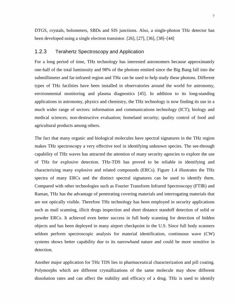
1.2.3 Terahertz Spectroscopy and Application

For a long period of time, THz technology has interested astronomers because approximately

one-half of the total luminosity and 98% of the photons emitted since the Big Bang fall into the

submillimeter and far-infrared region and THz can be used to help study these photons. Different

types of THz facilities have been installed in observatories around the world for astronomy,

environmental monitoring and plasma diagnostics [45]. In addition to its long-standing

applications in astronomy, physics and chemistry, the THz technology is now finding its use in a

much wider range of sectors: information and communications technology (ICT); biology and

medical sciences; non-destructive evaluation; homeland security; quality control of food and

agricultural products among others.

The fact that many organic and biological molecules have spectral signatures in the THz region

makes THz spectroscopy a very effective tool in identifying unknown species. The see-through

capability of THz waves has attracted the attention of many security agencies to explore the use

of THz for explosive detection. THz-TDS has proved to be reliable in identifying and

characterizing many explosive and related compounds (ERCs). Figure 1.4 illustrates the THz

spectra of many ERCs and the distinct spectral signatures can be used to identify them.

Compared with other technologies such as Fourier Transform Infrared Spectroscopy (FTIR) and

Raman, THz has the advantage of penetrating covering materials and interrogating materials that

are not optically visible. Therefore THz technology has been employed in security applications

such as mail scanning, illicit drugs inspection and short distance standoff detection of solid or

powder ERCs. It achieved even better success in full body scanning for detection of hidden

objects and has been deployed in many airport checkpoint in the U.S. Since full body scanners

seldom perform spectroscopic analysis for material identification, continuous wave (CW)

systems shows better capability due to its narrowband nature and could be more sensitive in

detection.

Another major application for THz TDS lies in pharmaceutical characterization and pill coating.

Polymorphs which are different crystallizations of the same molecule may show different

dissolution rates and can affect the stability and efficacy of a drug. THz is used to identify

8

polymorph compounds and provide proof of authenticity of pills. Also the thickness of a coating

is very important for the proper release of the drug inside the body and it can affect the efficacy

and potential side effects of the drug. THz provides a non-destructive and non-contact method by

using the time of flight information contained in the waveform to measure the thickness of the

coatings of the pills.

In the food industry, THz spectroscopy is utilized to detect contaminants, pesticides, foreign

objects and the presence of antibiotics. The see-through capability of THz waves enables the

inspection of packaged food. As the moisture level is an indicator of the conditions of bacteria

growth, THz offers the potential to increase food safety by measuring the moisture level in the

food. Figure 1.5 shows the capability of THz in detection of foreign objects such as glass, plastic

and ceramic as small as a few mm in a chocolate bar.

Figure 1.5. Spectral characteristics of different ERCs in THz range, Figure adapted from Ref. [42]

9

Figure 1.6. Foreign objects detection in chocolate bars Figure adapted from Ref. [46]

Furthermore, with the combined advantage of see-through capabilities and excellent spatial

resolution, THz can also be utilized in NDE (Non-Destructive Evaluation) imaging. Specific

applications include detection of defects in insulation, plastic and ceramic materials, inspection

of corrosion in both metal and non-metallic substrates under insulation or coatings, fire damage

and other structure defects (cracks and delaminations) in composite materials, turbine blades and

art pieces inspection and restoration. THz-time domain systems are always employed in such

occasions based on the same principles of ultrasound in studying the structure of layers of

samples. CW systems are equally attractive since they can provide faster data rates.

In recent years, researchers are getting keen on exploring THz applications in medical area such

as skin, breast and liver cancer diagnosis and skin burn evaluation with promising results. These

applications are essentially based on the high sensitivity of THz waves to the presence of water.

In general, cancerous tissue tends to accumulate more water and display stronger THz absorption

in the spectrum. One of the big challenges currently is that the high water content in biological

samples and its high variability make measurement difficult. Also proper samples preparation

and measurement protocols need to be developed for THz experiments. Once applications in the

research phase are successful, THz would have a significant impact on early cancer diagnosis

and prevention.

1.3 Organization of Thesis

The thesis comprises five major sections:

10

Chapter 1 Introduction

Chapter 2 Experimental Instrumentation

Chapter 3 Methodology Development

Chapter 4 Results and Discussion

Chapter 5 Conclusion

In particular, we would like to elaborate on the experimental instrumentation and methodology

development in more detail since they have been the most challenging work in the entire project

and a comprehensive description will lead to a better understanding of the entire system.

In Chapter 2 we will present the experimental set-up at length including every subsystem that

performs heating, purging, cooling and ventilation for the system respectively. In the ensuing

Chapter 3 we will talk about how the system functions, what problems came up and how to

resolve them or optimize the situation. Next we will move on the discuss results obtained from

both spectral simulation and experiments, analyze the leads and accuracy and draw conclusions

accordingly.

Finally we will come to a summary of the whole research, evaluate the pros and cons of the THz

spectroscopy technology and its feasibility in industry, propose plans for improvements and cast

our vision into future prospects.

11

Chapter 2 Experimental Instrumentation

2.1 Introduction

In this chapter, we introduce the experimental set-up we designed for the high temperature

measurement of water vapor with THz spectroscopy. Figure 2.1 shows a schematic diagram of

the entire measurement system.

Figure 2.1. Schematic diagram of the experimental setup for high-temperature water vapor measurement with the THz spectroscopy.

The whole system comprises a couple of sub-systems, namely the light source, the gas cell, the

heating system, the purging system, and the ventilation and cooling system.

The THz beam leaving the emitter travels in an open path before reaching the window of the gas

cell. To eliminate the influence of room humidity, the entire optical path is enclosed in an airtight

box, purged constantly with dry air. The gas cell is a stainless steel cylinder 1 meter in length,

with 2 inch inner diameter, equipped with an Omega digital pressure gauge and several K-type

thermocouples. The two end windows are 5 mm-thick z-cut quartz disks and are tilted at an angle

of 45º. The gas cell body is wrapped with Omega Ultra-High Temperature Heating Tapes

(STH051-060) on top of which sits a thick blanket of fibre-glass as thermal insulation. A brief

description of the experimental procedure is as follows. Firstly we block the THz beam with a

piece of aluminum foil to collect the background signal. The gas cell is then filled with pure

nitrogen for reference measurement. To investigate the water spectrum at a certain water

12

concentration, we inject a calculated amount of distilled water though a septum fitting using a

gastight syringe. At the end of each water absorption measurement, we evacuate and flush the

gas cell with N2 gas 10 times to remove any residual water vapor. The cell is then backfilled with

the reference N2 to start the next test.

In the following sections, we will describe the design and function of each facility. Specific

experimental techniques and procedure will be explained along with the set-up description. A

more systematic testing procedure development will be elaborated in the next chapter.

2.2 The light Source

2.2.1 Continuous Wave THz Sources

As has been mentioned in the previous section, the recent advancement in optical technology

lead to the development of THz sources of all kinds. Among them, THz pulses based on femto-

second pulse lasers have been applied to objects imaging, and spectroscopy of gas, liquid and

solid materials. In particular the time-domain spectroscopy (TDS) system based on THz pulses

has been well-established as a laboratory standard for the THz spectroscopy and is widely

commercialized. The Fourier transformation is applied to the time-domain data in a THz-TDS

system to obtain frequency characteristics [47].

Over the past years enormous attention has been paid to tunable continuous wave (CW)

spectrometer which uses monochromatic sources. Compared with pulsed systems, CW systems

are more appropriate for imaging and spectroscopy because they provide a higher spectral

resolution (up to 100 MHz).

There are several requirements for the CW THz sources: they should provide high output power

to enable a wide dynamic range and the radiation should be monochromatic and tunable in

frequency. Moreover it is desirable to have a high degree of polarization for the characterization

of anisotropic samples. For microspectroscopy they also should serve as diffraction-limited THz

point sources, a property that can be best represented by M2 value [41].

13

2.2.2 Photomixing Technology

Photomixing denotes heterodyne difference frequency generation in high-bandwidth

photoconductors. The output of two continuous-wave lasers converts into terahertz radiation [26],

[37], [48]–[51].

S. Martens and scholars in Germany have described the principle and mechanism involved in the

photomixing technology [41]. A photomixer usually utilizes a tunable two-wavelength laser as a

source, which is stabilized by external cavities and includes an antireflection-coated commercial

laser diode, a collimator, a diffraction grating cylinder lens and a V-shaped mirror. In a tapered

optical amplifier the output beam is amplified to about 20-50 mW and is then focused on the

photomixer. The emitted THz radiation is then collimated by a hyperhemispherical Si lens that is

installed at the back of the LT-GaAs chip, which is used to collimate the beam. The optical

elements are made of Polyethylene terephthalate and Teflon lenses. Polarizers consist of wire

grids with thick wires and other wire grids serve as partially reflecting mirrors in the Fabry-Perot

setup [41].

Key advantages of photomixing systems include a high frequency resolution, spectral selectivity

and large signal-to-noise ratios. Typical applications utilizing these properties are high-resolution

gas spectroscopy, solid-state spectroscopy with the benefit of determining a sample’s complex

dielectric constant and spectrally sensitive imaging.

2.2.3 Operating Principles of TeraView CW Spectra 400

The basic principle of operation of the THz spectrometer is as follows. Two near-infrared diode

lasers are precisely tuned to offset their relative wavelengths, producing a beat signal at the

difference frequency when coupled into the same fiber. The output fiber is connected to a THz

photomixer emitter, converting this beat signal into coherent THz radiation. Similarly, the THz

beat signal is delivered as a reference to the THz photomixer receiver, which allows ultra-

sensitive coherent detection of the incident THz radiation, even at sub-nanowatt power levels.

This scheme is phase sensitive, compact, and requires no cryogenic cooling. The fiber-optic

scheme is shown in Figure 2.2.

14

Figure 2.2. The fiber optic scheme [53].

The THz spectrum is then achieved by incrementally varying the difference frequency via a

smooth, mode-hop free tuning of the near-infrared diode lasers, according to the temperature-

tuning technique (Figure 2.3a). The signal amplitude and phase are measured at each discrete

frequency point, from which the power can be derived. The spectrometer system comprises: two

distributed feedback (DFB) diode lasers, with electric temperature and current controllers; fiber

connections to all components; electronic source for terahertz emitter drive circuit; detection

amplifier system; one terahertz emitter (Figure 2.3b); one terahertz receiver (Figure 2.3c).

15

Figure 2.3. Difference frequency generation and detection: (a) Illustration of photomixing scheme. Two laser heads working at different temperatures have different frequencies. By controlling the temperature, the frequency difference between the two laser head can be adjusted. (b) Illustration of the THz generation scheme. (c) Illustration of the THz

detection scheme [53].

At each frequency point in the spectrum, a sinusoidal waveform is acquired using a time domain

sweep, executed using fiber stretching technology. This allows each frequency measurement to

be acquired in approximately 30 ms. When executing a frequency sweep, the scan time hold-off

is user variable, according to the desired signal-to noise ratio.

16

Terahertz pulsed instruments require little maintenance and are relatively compact and mobile as

there is no need for sophisticated cooling solutions. The power of the terahertz radiation used for

the measurements is below 1 μW.

2.3 Gas Cell

2.3.1 Gas Cell Design

The gas cell is made of a one meter long, two-inch-diameter stainless steel tube. The two end

windows are 5 mm-thick disks made of z-cut quartz. The windows are tilted at an angle of 45º as

calculations indicate that the power loss is less than 5% at this incident angle. The 45º is chosen

because it is close to Brewster’s angle which is calculated as 66º for the current case and it also

easy to be manufactured. Figure 2.4 shows the 3-D model of the gas cell assembly.

Figure 2.4. 3-D model of the gas cell assembly.

Flanges tilted at the same angle are used at both ends of the gas cell to mount the windows. To

seal the windows, we chose graphite gasket that is compatible with the window material in its

hardness and is resistant to high temperatures. Due to manufacturing difficulties, the surface of

the flange cannot be made perfect flat. This requires the bolting to be well-performed so that the

force on the flange disk can be evenly distributed. Figure 2.5 displays the section view of the

flange, gasket and window at one end of the gas cell. After the manufacturing and assembling,

we carried out air-tightness tests under both pressurized and vacuum conditions. It is confirmed

that the pressure inside the gas cell can stay stable without any significant drop for a considerable

period of time.

17

Figure 2.5. Section view of the one end of the gas cell.

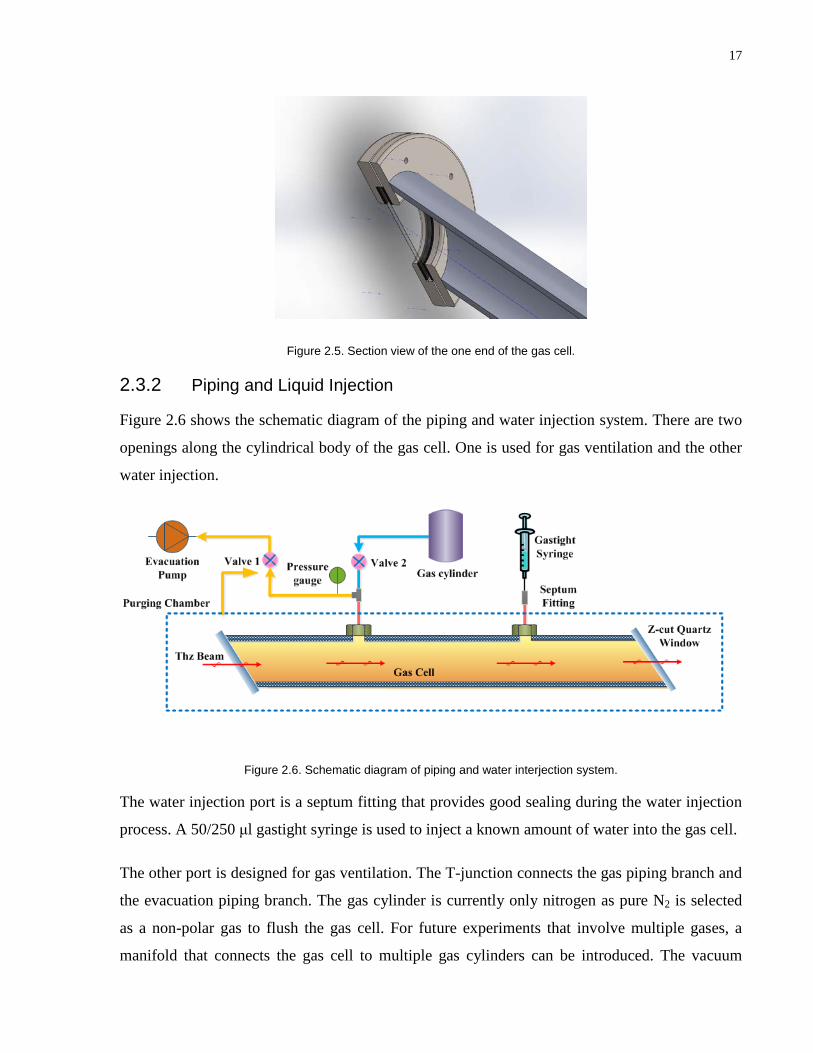
2.3.2 Piping and Liquid Injection

Figure 2.6 shows the schematic diagram of the piping and water injection system. There are two

openings along the cylindrical body of the gas cell. One is used for gas ventilation and the other

water injection.

Figure 2.6. Schematic diagram of piping and water interjection system.

The water injection port is a septum fitting that provides good sealing during the water injection

process. A 50/250 μl gastight syringe is used to inject a known amount of water into the gas cell.

The other port is designed for gas ventilation. The T-junction connects the gas piping branch and

the evacuation piping branch. The gas cylinder is currently only nitrogen as pure N2 is selected

as a non-polar gas to flush the gas cell. For future experiments that involve multiple gases, a

manifold that connects the gas cell to multiple gas cylinders can be introduced. The vacuum

18

pump serves for dual purposes in the current set-up: evacuation of the gas cell and the purging

and cooling of the optical path. By control of a three-way ball valve which connects the pump to

both the gas cell and the purging box, we are able to use the pump for different purpose under

difference circumstances.

2.3.3 Heating and Thermal Insulation

One of the most important features of the system is its achievement of the high temperature

measurement. The gas cell body is wrapped with Omega Ultra-High Temperature Heating Tapes

(STH051-060) on top of which sits a thick blanket of fibre-glass as thermal insulation. Two

heating tapes have been used, each of them controlled by a Variac. The heating system enables

the system to be warmed up to 500 ℃ and stay relatively stable at any temperature below Tmax.

Two K-type thermocouples are installed at the openings of the gas cell body to monitor the

temperature inside and provide real-time feedback for the temperature control.

2.4 Purging Chamber and Faraday Cage

2.4.1 Purging System

To investigate the water absorption spectra at different water concentrations inside the gas cell at

high temperatures, we have to keep the optical path dry and clean to remove the interference of

room humidity. To do this, we introduce the compressed air provided by the building where the

laboratory is located. Shown below is a demonstration of the purging scheme.

Figure 2.7. Purging chamber and compressed air ventilation scheme.

19

A clear Acrylic chamber is built to enclose the whole optical system. A rotameter is used to

control the volume flow rate of the compressed dry air for purging. The air flushes through the

chamber from both ends of the box and exits from the middle of the lid. Four humidity indicators

are placed at different positions in the chamber to ensure that the humidity is controlled well

below the atmospheric level.

2.4.2 Compressed Air Cooling

The compressed air that is used for purging also serves as a cooling medium to keep the

temperature of the chamber within acceptable limits. The optical sensor, especially the emitter

and receiver which are placed inside the purging box, are extremely delicate and high-

maintenance. The ambient temperature they are exposed to has to be kept at around 20-40℃. As

the radiation of the heated gas cell is constantly increasing the air temperature inside the purging

chamber, the flush air is not only removing the humidity but also the excessive heat. Figure 2.8

illustrates how the cooling scheme works.

Figure 2.8. Compressed air cooling for the optical system inside the purging chamber.

To mitigate the radiation heat transfer from the blazing body of the gas cell, we place two

thermal baffles between the gas cell and the optical heads. The material of the baffle plates is

calcium sulfide and they are 10 mm in thickness. A one-inch hole is chiseled on each plate to

allow the propagation of the THz beam. The compressed air enters the purging box from the left

and right ends, flows though the holes, travels along the gas cell and exits from the multiple tiny

20

openings on the purging box. The warm air is thus constantly exhausted from the chamber with

fresh cool air coming as replacement.

2.4.3 Faraday Cage

Tests have shown that the system is susceptible to ambient electromagnetic interference, which

will be discussed in detail in section 3.3. Therefore we built a Faraday cage that protects each

optical head, especially the receiver, from the E/M influence. The schematic diagram of the

Faraday cage is shown in Figure 2.8. It is achieved by wrapping each optical head with

aluminum foil and grounding it with a thin wire.

Note that the current Faraday cage is a modified version of a previous larger cage. Instead of

using two small cages to enclose the optical heads separately, we originally wrapped the whole

purging box with a seamless layer of Al foil. The large cage worked well in reducing the E/M

interference and improving the quality of the signal. However the heat dissipation was

significantly affected by the cage that it is hard to maintain the temperature close to the optical

heads to be below 40℃. Furthermore the plastic lid warped and melted due to the overheating

and repulsive odor was emitted from the melting material that consequently affected the water

spectrum. Therefore we removed the large cage and designed the current small separate cages

that perform equally well in signal improvement without causing any overheating.

2.5 Summary

In this chapter, we described the design and function of the experimental set-up. The whole

measurement system consists of the light source, which is a continuous wave THz spectrometer,

the 1-m long stainless steel gas cell, the heating and thermal insulation, the piping and water

injection, the compressed air purging and cooling system and the Faraday cage. The system

enables the measurement of the THz absorption spectra water vapor of different concentrations

at temperatures from room temperature to 500℃.

21

Chapter 3 Method Development

3.1 Introduction

In this chapter, we will focus on the method development for the THz spectroscopic

investigation on water vapor absorption. The THz spectrometer we purchased from TeraView

was originally fabricated as a standard product that aims to measure the transmission within the

path-length of 20 cm. In the present study, we extended the path-length to 120 cm which requires

a certain extension of the optical fiber connecting the receiver/emitter to the laser. However, this

modification to the system doesn’t come without a cost. The power amplitude dropped to 0.001

of its original value due to the diffraction of THz beam. Normally as the frequency goes higher,

the power drops accordingly. Fortunately the frequency range (below 1 THz) we are focusing for

the current study has relatively high power signal.

Since the technology is still in its infancy, the modification of the system further adds to its

unpredictability. The current research is largely devoted to method development; considerable

efforts have been spent on identifying the issue, trouble-shooting and finding approaches to

mitigate or resolve the problem before commencing the real investigation.

3.2 Development of Testing Procedure

3.2.1 System Warm-up and Stabilization

One important character about a THz system is its repeatability. The THz spectrometer we

acquired proves to have good repeatability as has been demonstrated in its Site Acceptance Test.

However, in our application where multiple scans are required for the averaging and analysis,

highly repeatable spectra are needed that could suppress the noise. But for the sake of saving

time, we would use single scan as it also provides a good enough SNR. In the previous tests, we

found it is hard for the system to produce repeatable data right after it is turned on. It needs a

considerable time to warm up and stabilize. This is due to the fact that the physical state of the

fiber stretcher that is crucial to accurate time delay control is dependent on the time of its

operation. Usually it takes a couple of hours or even a whole night to reach a steady state. Figure

3.1 shows the repeatability of the signal before and after the system reaches its stable state.

22

Figure 3.1. (a) Screenshots of the power output of the system before warm-up. (b) Power output of the system after warm-up.

The screenshots on the top display the difference in the repeatability of the power output

between the system in its pre-warmup and post-warmup states. As can be observed, the unstable

state on the top presents very fluctuating patterns in the spectra; the etalon fringes are highly

non-repeatable in the sequential tests. As a consequence, the averaged spectrum can be very

noisy after obtaining multiple scans of the non-repeatable data. By contrast, the screenshot at

Figure 3.1 (b) shows the spectra after the system is stabilized. The etalon fringes in adjacent tests

coincide with one another well with no apparent discrepancy, leading to minimal noise in the

averaged data.

Therefore, before collecting data for analysis in each test, we turn on the system a day

beforehand and run the warm-up scans for a whole night to make sure it becomes fully stabilized

23

once we kick off the test. To prevent the system from being worn down due to over-operation,

we set the emitter bias at 0.0 V during the system warmup and change it back to 0.55 V when

starting the data collection.

3.2.2 Background Measurement

The raw data we obtained from the spectrometer is THz power. To observe the absorbance

spectrum we have to carry out some subtractive calculations and data post-processing. To do this,

we employ the following equation,

0

ln IAI

= −

(1)

Where A is the absorbance,

I and I0 mean the signal and reference intensity respectively.

We employ the equation in the experiments and divide the signal with reference for each test.

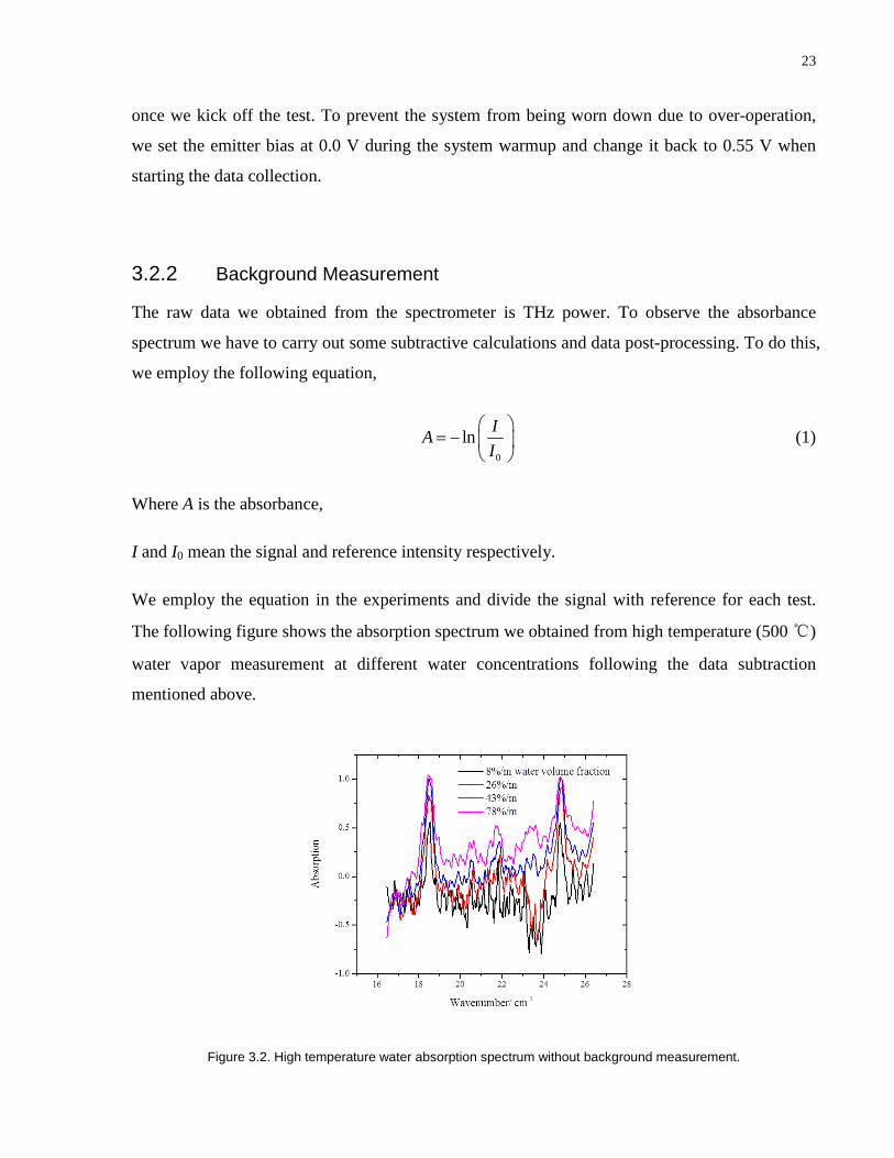
The following figure shows the absorption spectrum we obtained from high temperature (500 ℃)

water vapor measurement at different water concentrations following the data subtraction

mentioned above.

Figure 3.2. High temperature water absorption spectrum without background measurement.

24

As can be observed in Figure 3.2, the spectrum turned out to be extremely noisy; the spectral

baselines which should be coinciding or at least close to each other are scattered in a random

manner on the plot. It is hard to carry out further calculation and analysis based on the current

spectra. Therefore, we introduce the background measurement. Instead of going straight into

reference and signal collection, we set off each test with the measurement of background noise.

This is achieved by blocking the receiver with a thin layer of aluminum foil so that the THz

beam couldn't be detected and only the ambient noise signal is collected. Thus rather than

directly dividing the signal with reference, we subtract each value with background noise, as

given by the equation below,

noise

0 noise

ln I IAI I

−= − −

(2)

where Inoise stands for the power intensity of background noise.

Figure 3.3. High temperature water absorption spectrum with background measurement.

In Figure 3.3 we perceive the difference the measurement of background noise had on the high

temperature water. Not only do the baselines coincide with one another, but they also appear

much cleaner in the whole absorption spectrum. Therefore, we apply the baseline measurement

in the tests and carry out the spectral calculations and analysis accordingly.

25

3.2.3 Baseline Drift and Reference Measurement

The water absorption signal in each test is referred to a reference signal which is obtained by

measuring the absorption spectrum of the gas cell filled with nitrogen. The gas cell is evacuated

and flushed with dry N2 for 10 times to remove any residual water from the previous test.

Previously, we started off each set of tests by measuring the background noise and then the N2

reference. Each of the following water tests was referred to the reference test conducted at the

beginning. The results we obtained from this procedure can be found in figure 3.3. The baselines

of the spectra are slant and keep drifting upwards as we increase the water concentration of the

gas cell.

To investigate this phenomenon, we performed repetitive reference tests and refer each reference

to the first reference test to observe the change in the baseline over a period of time. The results

are shown in the figure below.

Figure 3.4. Spectral baseline drift with the time.

In figure 3.4, the bold lines are filtered spectral plots as opposed to the raw data in the back. As

all the reference data are referred to reference 1, we could see as time elapses the baseline tends

to climb upwards. Such phenomenon might be caused by the intrinsic power drift with time in

the system. To mitigate the influence of such systematic defect, we reduce the time interval

26

between the reference and signal tests by conducting a reference test for each humidity test.

Figure 3.5 shows the difference the improvement in the testing procedure had on the quality of

the spectrum.

Figure 3.5. (a) Slanted baseline due to power drift over-time. (b) Rectified baseline after designating reference for each signal test.

The change in the testing procedure makes a significant difference in the baseline of the spectra;

after conducting a reference test for each humidity test, we are able to rectify the tilted baseline

and move on with curve-fitting and analysis.

27

3.2.4 Water Signal Measurement

The water signal measurement is carried out after each reference test. The experimental

procedure is, firstly close the pump valve, leave the gas cell in vacuum condition and record the

pressure value. Then open the valve connecting the septum fitting and inject a known amount of

water (range: 30 μl-450 μl) with a gastight syringe. Wait at least half a minute for the water to

fully evaporate and the pressure to stabilize. Record the pressure again and the increase in the

pressure corresponds to the partial pressure of water vapor or the water volume fraction inside

the gas cell which should be consistent with the amount of water injected.

After the water injection, we fill the gas cell back with nitrogen until it reaches atmospheric

pressure. Then we start the scans. Note that in the initial tests when we raised the temperature,

the water condensation on the gas cell windows was so severe that it was extremely difficult for

the THz beam to pass though the gas cell and get detected at the other end. This is due to the

large temperature difference between the two sides of the gas cell windows. However as the

temperature gets high enough, usually over 120 ℃ , the condensed water would vaporize

completely and the test could be conducted smoothly. Therefore it is highly important that we

inject the water after the gas cell is fully warmed up and the temperature inside is stabilized.

3.3 Effect of Ambient E/M interference

3.3.1 Day-night Fluctuation in Signal Quality

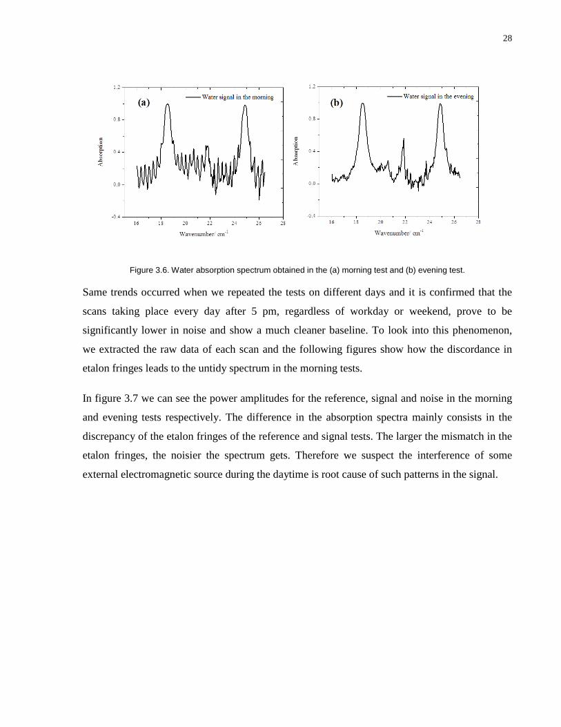
As we ran tests throughout the day, we found an intriguing phenomenon that the scans done

during daytime and evening produce completely different results; the data acquired during the

day turns out to be very noisy while evening tests give us a much cleaner spectrum. Figure 3.6

illustrates how the signal appears totally different in the morning (Figure Figure 3.6 (a)) and the

evening tests (Figure 3.6 (b)). The experimental conditions are kept exactly the same for both

tests, the gas cell temperature being 500 ℃ and the water volume fraction 69.5%.

28

Figure 3.6. Water absorption spectrum obtained in the (a) morning test and (b) evening test.

Same trends occurred when we repeated the tests on different days and it is confirmed that the

scans taking place every day after 5 pm, regardless of workday or weekend, prove to be

significantly lower in noise and show a much cleaner baseline. To look into this phenomenon,

we extracted the raw data of each scan and the following figures show how the discordance in

etalon fringes leads to the untidy spectrum in the morning tests.

In figure 3.7 we can see the power amplitudes for the reference, signal and noise in the morning

and evening tests respectively. The difference in the absorption spectra mainly consists in the

discrepancy of the etalon fringes of the reference and signal tests. The larger the mismatch in the

etalon fringes, the noisier the spectrum gets. Therefore we suspect the interference of some

external electromagnetic source during the daytime is root cause of such patterns in the signal.

29

Figure 3.7. Power amplitude of one sample tests and the resulting absorption spectrum: (a) Power amplitude data for morning test on 43%/m water at 500 ℃. (b) Absorption spectrum for the morning test. (c) Power amplitude data for

evening test on 43%/m water at 500 ℃; (d) Absorption spectrum for the evening test.

3.3.2 Introduction of Faraday Cage

In order to reduce the impact of ambient E/M interference, we built a Faraday cage around the

measurement system. The cage is made of a layer of aluminum foil which is wrapped seamlessly

around the purge box, shielding the system inside against any external E/M interference. The

Faraday cage is grounded with a thin copper wire. Figure 3.8 and 3.9 show the experimental set-

up before and after adding the Faraday cage.

30

Figure 3.8. High temperature water measurement system without Faraday Cage.

Figure 3.9. High temperature water measurement system with Al foil Faraday cage.

To investigate the effect of the Faraday cage, we set the system running day and night

continuously for a whole week and use the root mean square (RMS) method to analyze the

fluctuation of the data. The Faraday cage was used at the beginning and removed for a few days

31

and put back on for the rest of the test. Figure 3.10 illustrates how the RMS of data varies with

time.

Figure 3.10. RMS performance of the system during the whole-week operation.

In figure 3.10, the blue dots represent the tests done with the Faraday cage while the green ones

are obtained after removing the Faraday cage. The test started from 1st May and ended on 7th

May. The day and night time is denoted by the light and dark background. We can distinguish

the day-night cyclic variations in the RMS value and the quality of signal without the cage

appears much inferior to that with the cage; the fluctuation in RMS without the cage is much

higher than that with the cage. Figure 3.11 further demonstrates the difference the Faraday cage

has on the signal quality.

32

Figure 3.11. (a) RMS performance of the system with Faraday cage (b) RMS performance of the system without Faraday cage.

As we can observe from the figures above, in both cases the signal during the day is much

noisier than it is at night. Applying the Faraday cage which serves to block the external E/M

interference, the noise during both day and night is significantly lower than when the cage is

removed. Therefore we conclude that the Faraday cage is necessary in improving the signal

quality and lowering the noise.

33

One problem imposed by the Faraday cage is the heat dissipation of the system. The reflective

metal surface provides a layer of thermal insulation for the system that severely affects the

original cooling and ventilation. The temperature inside the purging chamber immediately goes

up, making it hard to control the temperature surrounding the optical heads below 35 ℃. Thus

instead of wrapping the whole purging box with aluminum foil, we made two small Faraday

cages covering only the emitter and receiver without affecting the heat transfer of the system

(See figure 3.12 for illustration). It has been tested and confirmed that the small separate cages

have the same effect on improving the signal quality.

Figure 3.12. Mini Faraday cage on the receiver.

3.4 Data Processing Techniques

3.4.1 Multiple scans, Averaging and Subtraction

After running the tests and exporting the raw THz power amplitude data, we move on to process

and analyze the data. According to the principles of measurement, the noise of the data is

inversely proportional to the number of repetitive measurement by a factor of n , where n is the

number of scanning. Therefore as a balance between the reduction of noise and the time spent on

each test, we choose to run 10 repetitive scans for each experimental condition and average the

data.

34

The next step is to divide the signal from the reference data. Equation (2) in section 3.2.3

indicates how the absorbance is calculated from the power signal.

3.4.2 Techniques for Removing Etalon Fringes

When we first plot out the absorbance spectrum, it appears extremely noisy most of the time. It is

hard to carry on with further analysis with such data. Therefore smoothing or denoising is needed

to process the data and make it analyzable. One of the most efficient techniques is Fast Fourier

Transform (FFT). Figure 3.11 compares the absorption spectrum before and after the FFT

filtering.

Figure 3.13. Water absorption spectra for different humidity levels (a) before and (b) after FFT filtering.

The reason why we choose the FFT method among all other smoothing techniques is because the

oscillation of the etalon signal in the water spectrum has a distinct frequency. If we do the FFT

analysis on a given spectrum, we would find, as is shown on the left of figure 3.12, the etalon

signal has a dominant frequency of 3.02. Therefore, we apply the low pass filter and set the

cutoff frequency at different values ranging from 1.0-3.5. The plot on the right of figure 3.12

displays how different cutoff frequency affects the filtering results. The optimal cutoff frequency

is found to be approximately 3.

35

Figure 3.14. (a) FFT analysis in water spectrum signal processing. (b) FFT filtering results with different cutoff frequency.

Since applying the filtering of any kind to the data inevitably leads to a compromise in its

accuracy, we are more intent on improving the quality of raw signal than doing signal processing.

As has been mentioned in section 3.3, doing tests in the evening usually produces good results in

terms of signal quality. We thus are inclined to use the evening data if it is good enough without

applying any signal processing.

3.4.3 Curve Fitting and Peak Area Calculation

We carry out our investigation on the spectrum signature of water vapor and its significance in

water quantification based on the Beer Lambert Law which is given by [49],

P0 tot( / ) exp[ ( ) ( )]I I XP S T Lυ υ φ υ= − (3)

or,

P0 totln( / ) ( ) ( )I I XP S T Lυ υ φ υ− = (4)

where 0( / )I I υ is the measured signal intensity ratio; X is the mole fraction of the absorbing

species; Ptot is the total absolute system pressure in atm; P ( )S Tυ is the line strength of the

transition in cm-2atm-1; L is the absorption path length in cm; ( )φ υ is the line shape function of

the transition in cm-1.

36

The formula on the left denotes the absorbance whose integration is given by,

P P0 tot totln( / ) ( ) ( ) ( ) ( )I I XP S T L XP S Tυ υ υφ υ φ υ− = =∫ ∫ ∫ (5)

where

( ) 1φ υ =∫ (6)

Thus we obtain,

P0 totln( / ) ( )PeakArea I I XP S Tυ υ= − =∫ (7)

where 0ln( / )I I υ−∫ stands for the absorbance peak area and totXP combined stands for the

volumetric concentration of species. As P ( )S Tυ is fixed at a particular wavenumber, the peak area

is in linear correlation with the gas concentration.

To verify the theory, we need to analyze the water spectrum from both simulation and

experiments based on curve-fitting and area integration. According to the theory in spectroscopy,

we apply Voigt-fitting to the absorbance peaks. OriginPro 8.0 is used as the data analysis tool for

curve-fitting and area calculations. Figure 3.13 show the curve-fitting results for simulation and

experimental data. In Chapter 4 results and discussion, we will compare the simulation line

strength with the experimental results in detail.

Figure 3.15. Voigt fitting results for (a) simulation and (b) experimental water absorption spectrum at 500 ℃ and at 0%/m water volume fraction.

37

3.5 Summary

In this chapter, we presented the method development of current research, which comprises a

major part of the whole project. As the application of THz technology in gas spectroscopy is still

in its infancy and the system we purchased has been modified for the current study, we have

been encountering many an issue along the way.

On the hardware side, we have dealt with the system stabilization, the background noise effect,

the power drift and the E/M interference to the system. On the software side, we addressed the

signal processing and data analysis. On the whole, we are able to identify various problems

coming up during the tests, carry out trouble-shooting and finding the best possible way to

optimize the situation.

38

Chapter 4 Results and Discussion

4.1 Introduction

In this chapter, we will present and discuss the results obtained from the experiments following

the experimental procedure and data analysis method developed in the previous chapters. The

results consist of two categories, the spectral simulation and the experimental study. Theoretical

simulations were carried out first by employing the commercial spectral simulator SpectraCalc

which draws on data from the 2008 edition of HITRAN database. The simulation results

essentially serve as a guidance for us to locate and pinpoint the new peaks which emerge at high

temperatures and also to justify the experimental outcome. By comparing the experimental

results with simulation, we will be able to find the correlation between the water concentration

and peak absorption features. Beam scattering experiments were conducted as an auxiliary test to

justify the motivation mentioned in the first chapter. The characteristics of the emerging new

peaks would also be discussed. These results will help us in the use of THz spectroscopy to

quantify water vapor produced from combustion in industrial processes.

4.2 HITRAN Spectral Simulation

4.2.1 Modelling of Water Spectrum in Gas Cell

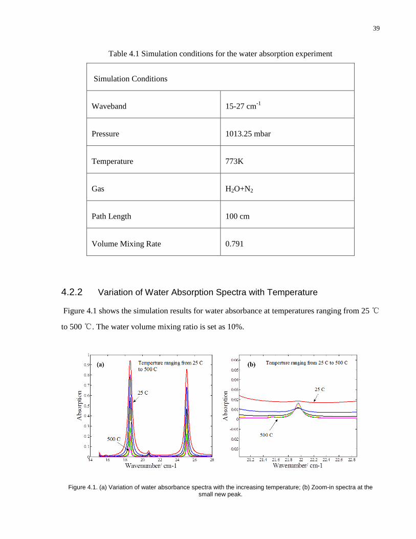
The simulation conditions are set exactly the same as the experimental study. Details of the

simulation settings are displayed in Table 4.1.

Although we control the crucial factors exactly the same as the experimental condition, the

current simulation, as of the experimental study, is in fact a simplified version of the real

industrial processes. For one thing, the open optical path is constantly purged with dry air in the

experiment and is eliminated in the spectral simulation. Whereas in industry, the path might be

exposed to room humidity and the spectrum would change to some extent accordingly. This will

be further addressed in the coming sections and both simulation of single gas cell and 2-cells are

carried out and compared to investigate the possible challenges in industry.

39

Table 4.1 Simulation conditions for the water absorption experiment

Simulation Conditions

Waveband 15-27 cm-1

Pressure 1013.25 mbar

Temperature 773K

Gas H2O+N2

Path Length 100 cm

Volume Mixing Rate 0.791

4.2.2 Variation of Water Absorption Spectra with Temperature

Figure 4.1 shows the simulation results for water absorbance at temperatures ranging from 25 ℃

to 500 ℃. The water volume mixing ratio is set as 10%.

Figure 4.1. (a) Variation of water absorbance spectra with the increasing temperature; (b) Zoom-in spectra at the small new peak.

40

In the figure we can observe the peaks due to rotational transmission of water molecules and that

as the temperature goes up the large peaks at 18.57 cm-1 (0.573 THz) and 24.53cm-1 (0.88 THz)

shrink with the temperature in both their heights and widths. The small peak at 21.94cm-1 (0.667

THz) emerges at high temperature and grows as the temperature increases.

4.2.3 Variation of Water Absorption Spectra with Humidity

According to the Beer-Lambert law, the water absorbance peak area is in proportion to the water

concentration. We thus performed a series of simulation at the same temperature 500 ℃ with

water concentration varying from 5%-m to 80%-m which corresponds to 1.25%-m to 20%-m in

a typical 4-meter-long off-gas duct in the industrial furnace. Figure 4.2 shows the results of

variation of water absorbance with humidity.

Figure 4.2. Effect of water volume fraction on the water absorbance spectrum

In the figure, the water absorbance peak is growing monotonically with the increasing humidity.

In the absorption spectrum the large peaks are prone to saturation at higher concentrations;

instead of growing higher, the absorption peaks stop at 1 and start extending horizontally and

become fatter. By contrast, in the absorbance spectrum, the peak keeps growing upwards with

the humidity instead of stretching too much horizontally. Same trend applies to both the large

41

and small peaks. Another remarkable feature is the rise of baseline. As the humidity increases,

the water spectrum goes up and encloses the curves underneath which is due to the tail of the

major peaks.

4.2.4 Correlation between Absorbance Peak Area and Water Concentration

Following the methodology described in Chapter 3, we perform curve fitting and analysis for the

water absorbance spectrum. Figure 4.3 demonstrates the sample calculation for the large peak at

18.57 cm-1 (0.557THz).

Figure 4.3. Sample calculation for the large peak at 18.57 cm-1(0.573 THz).

The transmittance data obtained from the spectral simulator is processed based on equation (2) to

get the absorbance spectrum. Then we use two different means to perform curve-fitting for the

absorbance peaks. The curve-fitting shown on the top is achieved by the multiple-peaks Voigt

fitting algorithm in OriginLab. With the fitted curve we do the integration and get the peak area.

Plotting out the peak area against the water concentration we perceive a very near linear

correlation (details shown in Figure 4.5). The slope is calculated to be 0.04458 and the adjusted

R square value is approximating 1, indicating the goodness of fitting is very satisfactory.

The fitting at the bottom is achieved by a self-developed subroutine written in Matlab. The Voigt

profile is generated by an approximation of the Voigt function. Instead of curve-fitting all four

42

peaks in the whole spectrum, the fitting is applied to individual peaks and integration obtained

accordingly. Similar results of the peak area-water concentration correlation is observed

following this curve-fitting method. As the accuracy of the fitting is better with the OriginLab

method, we choose to use the OriginLab software to perform the curve-fitting and further

analysis. The same sample calculations for the small new peak at 0.667 THz is shown in figure

4.4. The linear correlation of the water concentration and peak area for both the large and small

peaks are displayed in figure 4.6 (a) and (b) respectively.

Figure 4.4. Sample calculation for the small new peak at 21.94 cm-1(0.667 THz).

43

Figure 4.5. Linear fitting of the water concentration-peak area correlation for (a) Large absorbance peak at 0.557 THz.

(b) Small peak at 0.667THz.

4.2.5 Two-cell simulation and peak area-concentration correlation

To explore the possibility of industrial application, we carry out the 2-cell simulation as a

simplified version of the real industry. Shown below is the schematic diagram of the 2-cell

simulation.

Figure 4.6. Schematic diagram of the two-cell water absorption simulation.

The 0.2 m room temperature cell is recognized as the open path the laser travels outside the

furnace. The 1 m high temperature cell is seen as the harsh environment in the furnace. The

humidity for the room cell is selected as the atmospheric humidity on a typical day (23 ℃, 1.3 %

water) and the humidity inside the high temperature cell is varied from 5%-90%.

44

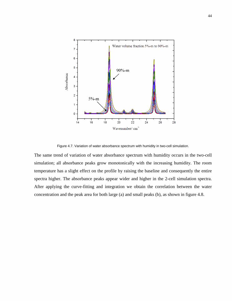
Figure 4.7. Variation of water absorbance spectrum with humidity in two-cell simulation.

The same trend of variation of water absorbance spectrum with humidity occurs in the two-cell

simulation; all absorbance peaks grow monotonically with the increasing humidity. The room

temperature has a slight effect on the profile by raising the baseline and consequently the entire

spectra higher. The absorbance peaks appear wider and higher in the 2-cell simulation spectra.

After applying the curve-fitting and integration we obtain the correlation between the water

concentration and the peak area for both large (a) and small peaks (b), as shown in figure 4.8.

45

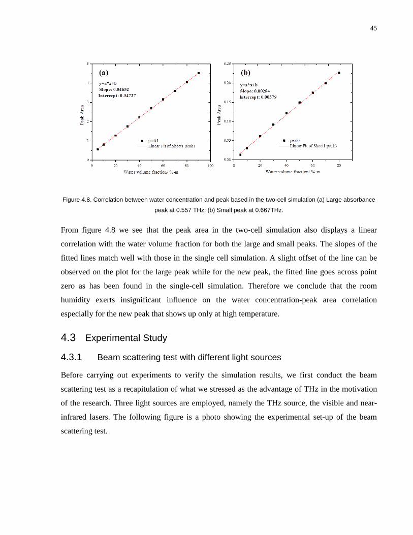
Figure 4.8. Correlation between water concentration and peak based in the two-cell simulation (a) Large absorbance

peak at 0.557 THz; (b) Small peak at 0.667THz.

From figure 4.8 we see that the peak area in the two-cell simulation also displays a linear

correlation with the water volume fraction for both the large and small peaks. The slopes of the

fitted lines match well with those in the single cell simulation. A slight offset of the line can be

observed on the plot for the large peak while for the new peak, the fitted line goes across point

zero as has been found in the single-cell simulation. Therefore we conclude that the room

humidity exerts insignificant influence on the water concentration-peak area correlation

especially for the new peak that shows up only at high temperature.

4.3 Experimental Study

4.3.1 Beam scattering test with different light sources

Before carrying out experiments to verify the simulation results, we first conduct the beam

scattering test as a recapitulation of what we stressed as the advantage of THz in the motivation

of the research. Three light sources are employed, namely the THz source, the visible and near-

infrared lasers. The following figure is a photo showing the experimental set-up of the beam

scattering test.

46

Figure 4.9. Experimental set-up for the beam scattering test with different light sources.

In the beam scattering testing system, the emitters and receivers of the three light sources are

placed at the right and left side of the purging box respectively. In the middle there put a plastic

tube with a vibrating sieve dropping fine Talcum powder with an estimated particle size of 0.01

mm.

As the purpose of the beam scattering test is to verify THz capability of penetrating dusty

environment, we select four typical frequencies, namely 0.2 THz, 0.6 THz, 1.0 THz and 1.25THz

and carry out four tests accordingly to compare the transmittance in the THz domain with that in

the visible and near-infrared. Results are shown in figure 4.10 where the green dots denote the

THz beam, the red and blue lines stand for the visible and near-infrared respectively. The steep

dip of signal marks the beginning of the particle drop. As we can observe from all four plots, the

visible and NIR transmittance dropped to 50% of its original value due to beam scattering loss,

or particularly MIE scattering. Whereas for THz, especially in lower frequency, there is no or

only a slight dip of signal. At higher frequency some scattering occurred, but transmittance is

always at or above that of the Visible and NIR lasers. Note that due to limitations of the THz

instrument, at higher frequency the power drops significantly, see Figure 3.1, which leads to the

uncertainty of data at 1.0 THz and 1.25 THz.

47

Figure 4.10. Transmittance of the difference light sources in the beam scattering test.

4.3.2 Variation of Water Absorbance Spectra with Humidity

Here we start the investigation on the relationship between the water absorption spectra with the

increasing humidity. Measurements are carried out when the gas cell is heated up to 500 ℃ at the

water concentrations ranging from 8%-90%. Results are displayed in figure 4.11 and 4.12. In the

aspects of peak location and height, the experimental spectra show good agreement with the

simulation results.

48

Figure 4.11. Experimental water spectra varying with increasing humidity at 500 ℃.

Figure 4.12. Variation of water absorbance peak at 18.57 cm-1(0.573 THz) with humidity.

49

4.3.3 Experimental Correlation Between Absorbance Peak Area and Water Concentration

After obtaining high temperature water absorbance spectra at different humidity we move on to

analyze the correlation between the peak area and water volume fraction. The figure below

demonstrates the calculation procedure for the experimental data.

Figure 4.13. Sample calculation of experimental data for the large peak at 18.57 cm-1(0.573 THz): (a) Power amplitude data obtained from one scan. (b) Absorbance Spectrum. (c) Multiple peak Voigt Curve-fitting. (d)

Correlation between water volume fraction and peak area.

In figure 4.13 we first export the power signal data from the multiple scans. Averaging and

subtraction are done afterwards to obtain the absorbance spectrum. Then we come to the

multiple-peak curve-fitting and peak area integration. Finally the peak area is plotted against the

water concentration and as we expected, there exists a linear correlation between the two

according to the theoretical prediction. More repetitive tests are performed to confirm the results.

Figure 4.14 show the experimental results obtained from tests on different days and compare

them with the HITRAN prediction.

50

Figure 4.14. Experimental results versus HITRAN prediction of tests: (a) Correlation between injected water volume and peak area for peak at 0.557THz. (b) Correlation between injected water volume and peak area for peak at

0.753THz.

There is a good agreement between the experimental and theoretical results for the two large

peaks at 0.557 THz and 0.753 THz. If we do a linear fitting for the peak of interest (0.557 THz)

and compare the results with the predicted linear correlation, we found the slopes of the

experimental (0.04413) and simulation (0.04458) linear correlations match with each other

within 1%.

Due to low output power at the new peak position (0.67 THz), we used two parabolic mirrors

(one with 4’ focal length, the other 1’ focal length, with protected gold coating) to collimate the

THz beam and reduce the diffraction. Figure 4.15 illustrates the upgraded measurement system

layout. It is found that with the beam collimation the THz signal strength increase by 100 times.

As a consequence, the water absorbance spectra appear much cleaner and the small new peak

clearly visible, as can be observed in Figure 4.16. After the data processing we obtain the linear

correlation between the water concentration and the new peak area shown in figure 4.17. The

slope is calculated as 0.00307 which is about 8% different from the simulated value 0.00284.

This is a promising lead that sheds light on the possibility of quantifying high temperature water

vapor in industrial processes by small peak measurement.

51

Figure 4.15. THz high temperature water measurement system parabolic mirror upgrade.

Figure 4.16. High temperature water absorbance spectra measured after the system upgrade.

52

Figure 4.17. Experimental data for small peak at 21.94cm-1 (0.667 THz) and linear fitting results.

4.4 Summary

In this chapter, we present the results obtained from the spectral simulation and experimental

study. In both simulation and experiments, it is found that the strong absorption peaks at 0.557

THz (18.57 cm-1) and 0.753 THz (24.85 cm-1) shrink with the increasing temperature, and new

peaks at 0.667 THz (21.94 cm-1), 0.88 THz (29.04 cm-1) emerge at high temperature. This

phenomenon can be explained by the change in the rotational rates and state populations

triggered by the change in temperature. The absorbance spectra have been collected within the

frequency range of 0.5-0.8 THz at a series of humidity levels ranging from 8% to 70%. We

observed that absorbance peaks grow with the humidity. The areas underneath the peaks of

interest are calculated by integration and hence we are able to plot out the peak area against a

series of water concentrations.

For the gas cell humidity ranging from 5% to 78%, the absorbance peak area at 18.57 cm-1

(0.557 THz) and 24.85 cm-1(0.753THz) displays good linear correlation with the water

concentration, which can be justified by the Beer-Lambert Law. The simulation results are then

verified by experimental study; a clean linear correlation between the water concentration and

the absorbance peak area was found and displayed in figure 3b. The slopes of the experimental

(0.04413) and simulation (0.04458) linear correlations match with each other within 1%.

53

To increase the signal strength of the THz system, we added two parabolic mirrors for beam

collimation. The power is improved significantly and the experimental results for the small new

peak at 0.667 THz proved to be in good agreement with the theoretical prediction. Such leads

give us more confidence in the future industrial application.

54

Chapter 5 Conclusion

5.1 Summary

Terahertz (THz) radiation, which fills the gap in the electromagnetic spectrum between the

microwave and the infrared light, has the advantage of transmitting through gases with high

particle loading with reduced light scattering. THz has remained quite unexplored until most

recent years when fast advancements in photonics took place, making it possible to generate and

detect THz beams with much more efficiency.

In the current research, we focus on the measurement of water vapor at high temperatures using

THz spectroscopy. A monochromatic continuous wave THz source with wide tunable frequency

range and high resolution is employed. The heating system we established allows us to carry out

experiments at temperatures from room temperature to as high as 500 ℃. The gas cell is 1 meter

long and made of a stainless steel tube at the end of which mounted two z-cut quartz windows.

The optical path is constantly purged with dry air to remove the room humidity and also to

increase heat dissipation and keep the temperature inside the purging chamber stable. Two

separate Faraday cages are applied on the optical heads to block the E/M interference. The

system enables the measurement of water vapor of different concentrations at temperatures from

room temperature to 500℃.

As the application of THz technology in gas spectroscopy is still in its infancy, we encountered

many issues when carrying out our research. On the hardware side, we dealt with the system

stabilization, the background noise effect, the power drift and the E/M interference to the system.

On the software side, we addressed the signal processing and data analysis. Up to now, we are

able to identify various problems coming up during the tests, carry out trouble-shooting and

finding the best possible way to optimize the situation.

HITRAN simulation for frequency range 0.5-0.8THz is first carried out by employing the

commercial spectral simulator SpectraCalc which draws on data from the 2008 edition of

HITRAN database. Results indicate that the strong absorption peaks at 0.557 THz (18.57 cm-1)

and 0.753 THz ( 24.85 cm-1) shrink with the increasing temperature, whereas new peaks at 0.667

55

THz (21.94 cm-1), 0.88 THz (29.04 cm-1) emerge at high temperatures and grow as the

temperature increases.

For the gas cell humidity ranging from 5% to 78%, the absorbance peak area at 18.57 cm-1

(0.557 THz) and 24.85 cm-1(0.753THz) displays good linear correlation with the water

concentration, which is in consistence with the Beer-Lambert Law. The simulation results are

then verified by experimental study; a clean linear correlation between the water concentration

and the absorbance peak area was observed. The slopes of the experimental (0.04413) and

simulation (0.04458) linear correlations match with each other within 1%.

Two parabolic mirrors for beam collimation were added to increase the signal strength of the

THz system. The power is improved significantly and the experimental results for the small new

peak at 0.667 THz proved to be in good agreement with the theoretical prediction. Such leads

give us more confidence in the future industrial application.

5.2 Industrial application

In a typical industrial furnace, the optical path length is usually 4 meters. The water

concentration in a steel making plate ranges from 15%-25% which corresponds to 60%-100% in

a 1-m measurement system. The temperature is around 1200-1500 ℃ which is much higher than

what can be achieved in the current laboratory facility and beyond the calculation scope of

HITRAN.

As has been mentioned in the motivation, THz provides a non-destructive, in-situ off-gas

detection and analysis method. It also has the advantage over other light sources for being

capable of penetrating environment heavily-laden with particles. Many gaseous species have

spectral signatures in the THz range and among them, water vapor shows distinct absorption

lines that can be utilized for diagnostic purpose. Moreover, at high temperature, new absorption

peaks emerge in the water spectrum and grow with the increasing humidity. This feature makes it

possible to quantify water vapor in the furnace without the influence of the atmospheric humidity

in the optical path.

However, since the continuous wave THz technology is still immature, there are considerable

challenges that need to be addressed before its industrial application. For one thing, in the

56

industrial configuration, the optical path is too long for the THz beam to travel without suffering

significant diffraction. Parabolic mirrors could be used to improve collimation purpose which

will increase cost and add to the complexity. Another challenge is that the THz instrument is

extremely delicate and susceptible to the harsh environment and exterior E/M interference. The

lasers and optical heads must be placed in air-conditioned environment to ensure its good

performance. Also the strike of electric arc in a steel-making furnace poses substantial hazard for

the THz instrument and good E/M protection must be considered. Last but not least, the current

system is very bulky and heavy and can be extremely vulnerable to vibration and damage in the

industrial application. It is highly desirable to have a more compact and rugged system.

5.3 Current Challenges

The E/M interference on the system is one of the most indecipherable challenges under

investigation. Although the application of Faraday cage makes a difference in improving the

signal quality, the quality of the data is quite unpredictable and the day-night fluctuation in signal

still remains despite the presence of the Al shield. In order to obtain good data for analysis, we

are obliged to carry out evening tests as in general the evening data appear cleaner than day-time

data.

Although the power strength is improved substantially within the frequency range of interest, the

signal drops drastically beyond 0.8 THz, posing huge challenges for investigation at higher

frequency range.

5.4 Recommendations for Future Work

In the future study we would like to continue focusing on the explorative study in the laboratory

and also plan out field trials when opportunity comes.

The laboratory work includes exploring the temperature dependency of line strength and line-

width of water absorption peaks. Also, as the strengths of peaks like 0.557 THz and 0.753 THz

decrease with the increasing temperature and the strength of peaks at 0.667 THz and 0.88 THz

increase with temperature, it could be used to measure the temperature. Other combustion gases

such as CO will be investigated after some modification to the current facility.

57

For the filed trial, we would like to collaborate with the THz instrument supplier for the

development of a more compact and robust system and the improvement of its overall

performance. Once the technology is ready, we would install the system in the off-gas duct of a

furnace and test its performance in the real steel-making process.

58

References [1] T. Aizawa, T. Kamimoto, and T. Tamaru, “Measurements of OH radical concentration in combustion

environments by wavelength-modulation spectroscopy with a 1.55-micron distributed-feedback diode

laser.,” Appl. Opt., vol. 38, no. 9, pp. 1733–41, Mar. 1999.

[2] T. K. Balasubramanian, A. P. Mishra, and R. J. Kshirsagar, “Absorption intensities of rovibronic transitions

in the A-band of 16O2: Analysis and calculation of magnetic dipole and electric quadrupole contributions,”

J. Quant. Spectrosc. Radiat. Transf., vol. 133, pp. 91–98, Jan. 2014.

[3] S. I. Chou, D. S. Baer, and R. K. Hanson, “Diode laser absorption measurements of CH(3)Cl and CH(4)

near 1.65 micron.,” Appl. Opt., vol. 36, no. 15, pp. 3288–93, May 1997.

[4] J. Graul and T. Lilly, “Coherent Rayleigh-Brillouin scattering measurement of atmospheric atomic and

molecular gas temperature,” Opt. Express, vol. 22, no. 17, p. 20117, Aug. 2014.

[5] a. Grosch, H. Wackerbarth, O. Thiele, T. Berg, and L. Beckmann, “Infrared spectroscopic concentration

measurements of carbon dioxide and gaseous water in harsh environments with a fiber optical sensor by

using the HITEMP database,” J. Quant. Spectrosc. Radiat. Transf., vol. 133, pp. 106–116, Jan. 2014.

[6] R. M. Mihalcea, D. S. Baer, and R. K. Hanson, “Tunable diode-laser absorption measurements of NO(2)

near 670 and 395 nm.,” Appl. Opt., vol. 35, no. 21, pp. 4059–64, Jul. 1996.

[7] R. M. Mihalcea, D. S. Baer, and R. K. Hanson, “Diode laser sensor for measurements of CO, CO(2), and

CH(4) in combustion flows.,” Appl. Opt., vol. 36, no. 33, pp. 8745–52, Nov. 1997.

[8] V. Nagali, S. Chou, and D. Baer, “Tunable diode-laser absorption measurements of methane at elevated

temperatures,” Appl. Opt., vol. 35, no. 21, 1996.

[9] a. Padmanabhan, T. Tzanetakis, a. Chanda, and M. J. Thomson, “Study of pressure broadening effects of H2

on CO2 and CO in the near infrared region between 6317 and 6335cm−1 at room temperature,” J. Quant.

Spectrosc. Radiat. Transf., vol. 133, pp. 81–90, Jan. 2014.

[10] A. Pogány, O. Ott, O. Werhahn, and V. Ebert, “Towards traceability in CO2 line strength measurements by

TDLAS at 2.7µm,” J. Quant. Spectrosc. Radiat. Transf., vol. 130, pp. 147–157, Nov. 2013.

[11] D. M. Slocum, E. J. Slingerland, R. H. Giles, and T. M. Goyette, “Atmospheric absorption of terahertz

radiation and water vapor continuum effects,” J. Quant. Spectrosc. Radiat. Transf., vol. 127, pp. 49–63, Sep.

2013.

59

[12] D. M. Sonnenfroh and M. G. Allen, “Absorption measurements of the second overtone band of NO in

ambient and combustion gases with a 1.8-mum room-temperature diode laser.,” Appl. Opt., vol. 36, no. 30,

pp. 7970–7, Oct. 1997.

[13] J. Ge, R. Wang, S. Hu, N. Dai, D. Li, H. Ma, and G. Ma, “Investigation of the strengths of vapor rotational

absorption lines with different humidity by far infrared absorption spectra,” 2009, vol. 7385, p. 73851L–

73851L–11.

[14] H. Hoshina, T. Seta, T. Iwamoto, I. Hosako, C. Otani, and Y. Kasai, “Precise measurement of pressure

broadening parameters for water vapor with a terahertz time-domain spectrometer,” J. Quant. Spectrosc.

Radiat. Transf., vol. 109, no. 12–13, pp. 2303–2314, Aug. 2008.

[15] V. B. Podobedov, D. F. Plusquellic, and G. T. Fraser, “Investigation of the water-vapor continuum in the

THz region using a multipass cell,” J. Quant. Spectrosc. Radiat. Transf., vol. 91, no. 3, pp. 287–295, Mar.

2005.

[16] K. Su, L. Moeller, R. B. Barat, and J. F. Federici, “Experimental comparison of terahertz and infrared data

signal attenuation in dust clouds.,” J. Opt. Soc. Am. A. Opt. Image Sci. Vis., vol. 29, no. 11, pp. 2360–6, Nov.

2012.

[17] V. B. Podobedov, D. F. Plusquellic, K. E. Siegrist, G. T. Fraser, Q. Ma, and R. H. Tipping, “New

measurements of the water vapor continuum in the region from 0.3 to 2.7THz,” J. Quant. Spectrosc. Radiat.

Transf., vol. 109, no. 3, pp. 458–467, Feb. 2008.

[18] V. . Podobedov, D. . Plusquellic, and G. . Fraser, “THz laser study of self-pressure and temperature

broadening and shifts of water vapor lines for pressures up to,” J. Quant. Spectrosc. Radiat. Transf., vol. 87,

no. 3–4, pp. 377–385, Sep. 2004.

[19] Y. Yang, M. Mandehgar, and D. Grischkowsky, “Time domain measurement of the THz refractivity of

water vapor.,” Opt. Express, vol. 20, no. 24, pp. 26208–18, Nov. 2012.

[20] Y. Yang, A. Shutler, and D. Grischkowsky, “Measurement of the transmission of the atmosphere from 0.2 to

2 THz.,” Opt. Express, vol. 19, no. 9, pp. 8830–8, Apr. 2011.

[21] B. J. Drouin, S. Yu, J. C. Pearson, and H. Gupta, “Terahertz spectroscopy for space applications: 2.5–

2.7THz spectra of HD, H2O and NH3,” J. Mol. Struct., vol. 1006, no. 1–3, pp. 2–12, Dec. 2011.

[22] S. Eliet, A. Cuisset, M. Guinet, F. Hindle, G. Mouret, R. Bocquet, and J. Demaison, “Rotational spectrum of

formaldehyde reinvestigated using a photomixing THz synthesizer,” J. Mol. Spectrosc., vol. 279, pp. 12–15,

Sep. 2012.

60

[23] X. Xin, H. Altan, a. Saint, D. Matten, and R. R. Alfano, “Terahertz absorption spectrum of para and ortho

water vapors at different humidities at room temperature,” J. Appl. Phys., vol. 100, no. 9, p. 094905, 2006.

[24] S. Yu, J. C. Pearson, and B. J. Drouin, “Terahertz spectroscopy of water in its second triad,” J. Mol.

Spectrosc., vol. 288, pp. 7–10, Jun. 2013.

[25] S. Yu, J. C. Pearson, B. J. Drouin, M.-A. Martin-Drumel, O. Pirali, M. Vervloet, L. H. Coudert, H. S. P.

Müller, and S. Brünken, “Measurement and analysis of new terahertz and far-infrared spectra of high

temperature water,” J. Mol. Spectrosc., vol. 279, pp. 16–25, Sep. 2012.

[26] R. Engelbrecht, “A compact NIR fiber-optic diode laser spectrometer for CO and CO(2): analysis of

observed 2f wavelength modulation spectroscopy line shapes.,” Spectrochim. Acta. A. Mol. Biomol.

Spectrosc., vol. 60, no. 14, pp. 3291–8, Dec. 2004.

[27] a. Farooq, J. B. Jeffries, and R. K. Hanson, “CO2 concentration and temperature sensor for combustion

gases using diode-laser absorption near 2.7 μm,” Appl. Phys. B, vol. 90, no. 3–4, pp. 619–628, Jan. 2008.

[28] K. Kohse-Höinghaus, R. S. Barlow, M. Aldén, and J. Wolfrum, “Combustion at the focus: laser diagnostics

and control,” Proc. Combust. Inst., vol. 30, no. 1, pp. 89–123, Jan. 2005.

[29] X. Zhou, X. Liu, J. B. Jeffries, and R. K. Hanson, “Development of a sensor for temperature and water

concentration in combustion gases using a single tunable diode laser,” Meas. Sci. Technol., vol. 14, no. 8, pp.

1459–1468, Aug. 2003.

[30] B. L. Upschulte, D. M. Sonnenfroh, and M. G. Allen, “Measurements of CO, CO2, OH, and H2O in room-

temperature and combustion gases by use of a broadly current-tuned multisection InGaAsP diode laser.,”

Appl. Opt., vol. 38, no. 9, pp. 1506–12, Mar. 1999.

[31] T. Uno and H. Tabata, “In situ Measurement of Combustion Gas Using Terahertz Time Domain

Spectroscopy Setup for Gas Phase Spectroscopy and Measurement of Solid Sample,” Jpn. J. Appl. Phys.,

vol. 49, no. 4, p. 04DL17, Apr. 2010.

[32] K. Schäfer, J. Heland, D. H. Lister, C. W. Wilson, R. J. Howes, R. S. Falk, E. Lindermeir, M. Birk, G.

Wagner, P. Haschberger, M. Bernard, O. Legras, P. Wiesen, R. Kurtenbach, K. J. Brockmann, V. Kriesche,

M. Hilton, G. Bishop, R. Clarke, J. Workman, M. Caola, R. Geatches, R. Burrows, J. D. Black, P. Hervé,

and J. Vally, “Nonintrusive optical measurements of aircraft engine exhaust emissions and comparison with

standard intrusive techniques.,” Appl. Opt., vol. 39, no. 3, pp. 441–55, Jan. 2000.

[33] G. B. Rieker, H. Li, X. Liu, J. T. C. Liu, J. B. Jeffries, R. K. Hanson, M. G. Allen, S. D. Wehe, P. a. Mulhall,

H. S. Kindle, a. Kakuho, K. R. Sholes, T. Matsuura, and S. Takatani, “Rapid measurements of temperature

61

and H2O concentration in IC engines with a spark plug-mounted diode laser sensor,” Proc. Combust. Inst.,

vol. 31, no. 2, pp. 3041–3049, Jan. 2007.

[34] C. McDonagh, C. S. Burke, and B. D. MacCraith, “Optical chemical sensors.,” Chem. Rev., vol. 108, no. 2,

pp. 400–22, Feb. 2008.

[35] X. Liu and Y. Xu, “New rovibrational bands of the Ar–H2O complex at the ν2 bend region of H2O,” J. Mol.

Spectrosc., vol. 301, pp. 1–8, Jul. 2014.

[36] Y.-S. Lee, Principles of Terahertz Science and Technology: Proceedings of the International Conference,

Held in Mainz, Germany, June 5-9, 1979, vol. 170. Springer, 2009.

[37] A. Deninger, “State-of-the-Art in cw Photomixing Systems,” in International Conference on Fibre Optics

and Photonics, 2012, p. T3A.2.

[38] J. T. C. Liu, J. B. Jeffries, and R. K. Hanson, “Wavelength modulation absorption spectroscopy with 2 f

detection using multiplexed diode lasers for rapid temperature measurements in gaseous flows,” Appl. Phys.

B Lasers Opt., vol. 78, no. 3–4, pp. 503–511, Feb. 2004.

[39] J. T. C. Liu, J. B. Jeffries, and R. K. Hanson, “Large-modulation-depth 2f spectroscopy with diode lasers for

rapid temperature and species measurements in gases with blended and broadened spectra.,” Appl. Opt., vol.

43, no. 35, pp. 6500–9, Dec. 2004.

[40] X. Liu, J. B. Jeffries, R. K. Hanson, K. M. Hinckley, and M. a. Woodmansee, “Development of a tunable

diode laser sensor for measurements of gas turbine exhaust temperature,” Appl. Phys. B, vol. 82, no. 3, pp.

469–478, Dec. 2005.

[41] S. Martens, B. Gompf, and M. Dressel, “Characterization of continuous-wave terahertz sources: laser

mixing versus backward-wave oscillators.,” Appl. Opt., vol. 48, no. 29, pp. 5490–6, Oct. 2009.

[42] A. Redo-Sanchez, N. Laman, B. Schulkin, and T. Tongue, “Review of Terahertz Technology Readiness

Assessment and Applications,” J. Infrared, Millimeter, Terahertz Waves, vol. 34, no. 9, pp. 500–518, Jul.

2013.

[43] G. Whitenett, G. Stewart, H. Yu, and B. Culshaw, “Investigation of a Tuneable Mode-Locked Fiber Laser

for Application to Multipoint Gas Spectroscopy,” J. Light. Technol., vol. 22, no. 3, pp. 813–819, Mar. 2004.

[44] X. C. Zhang, “Terahertz wave imaging: horizons and hurdles.,” Phys. Med. Biol., vol. 47, no. 21, pp. 3667–

77, Nov. 2002.

62

[45] T. Kampfrath, M. Battiato, P. Maldonado, G. Eilers, J. Nötzold, S. Mährlein, V. Zbarsky, F. Freimuth, Y.

Mokrousov, S. Blügel, M. Wolf, I. Radu, P. M. Oppeneer, and M. Münzenberg, “Terahertz spin current

pulses controlled by magnetic heterostructures.,” Nat. Nanotechnol., vol. 8, no. 4, pp. 256–60, Apr. 2013.

[46] M. Tonouchi, “Cutting-edge terahertz technology,” Nat. Photonics, vol. 1, no. 2, pp. 97–105, Feb. 2007.

[47] T. Nagatsuma, A. Kaino, S. Hisatake, K. Ajito, and H. Song, “Continuous-wave Terahertz Spectroscopy

System Based on Photodiodes,” pp. 390–394, 2010.

[48] A. Dobroiu, M. Yamashita, Y. N. Ohshima, Y. Morita, C. Otani, and K. Kawase, “Terahertz imaging system

based on a backward-wave oscillator.,” Appl. Opt., vol. 43, no. 30, pp. 5637–46, Oct. 2004.

[49] M. G. Allen, “Diode laser absorption sensors for gas-dynamic and combustion flows.,” Meas. Sci. Technol.,

vol. 9, no. 4, pp. 545–62, Apr. 1998.

[50] N. Docquier and S. Candel, “Combustion control and sensors: a review,” Prog. Energy Combust. Sci., vol.

28, no. 2, pp. 107–150, Jan. 2002.

[51] V. Ebert, T. Fernholz, C. Giesemann, H. Pitz, H. Teichert, J. Wolfrum, and H. Jaritz, “SIMULTANEOUS

DIODE-LASER-BASED IN SITU DETECTION OF MULTIPLE SPECIES AND TEMPERATURE IN A

GAS-FIRED POWER PLANT,” vol. 28, pp. 423–430, 2000.

[52] “Lindarc | More,” 25-Aug-2014. [Online]. Available: http://www.more-oxy.com/en/products/lindarc.html.

[53] TeraView Documentation, received 7-August-2014 .

63

Appendices Appendix A. Humidity and Partial Pressure Conversion Table

Temperature/ K Water Volume/ μl Partial Pressure/ %

773.00 50.00 8.692984107

773.00 100 17.38596821

773.00 150 26.07895232

773.00 200 34.77193643

773.00 250 43.46492053

773.00 300 52.15790464

773.00 350 60.85088875

773.00 400 69.54387285

773.00 450 78.23685696

773.00 500 86.92984107

773.00 550 95.62282517

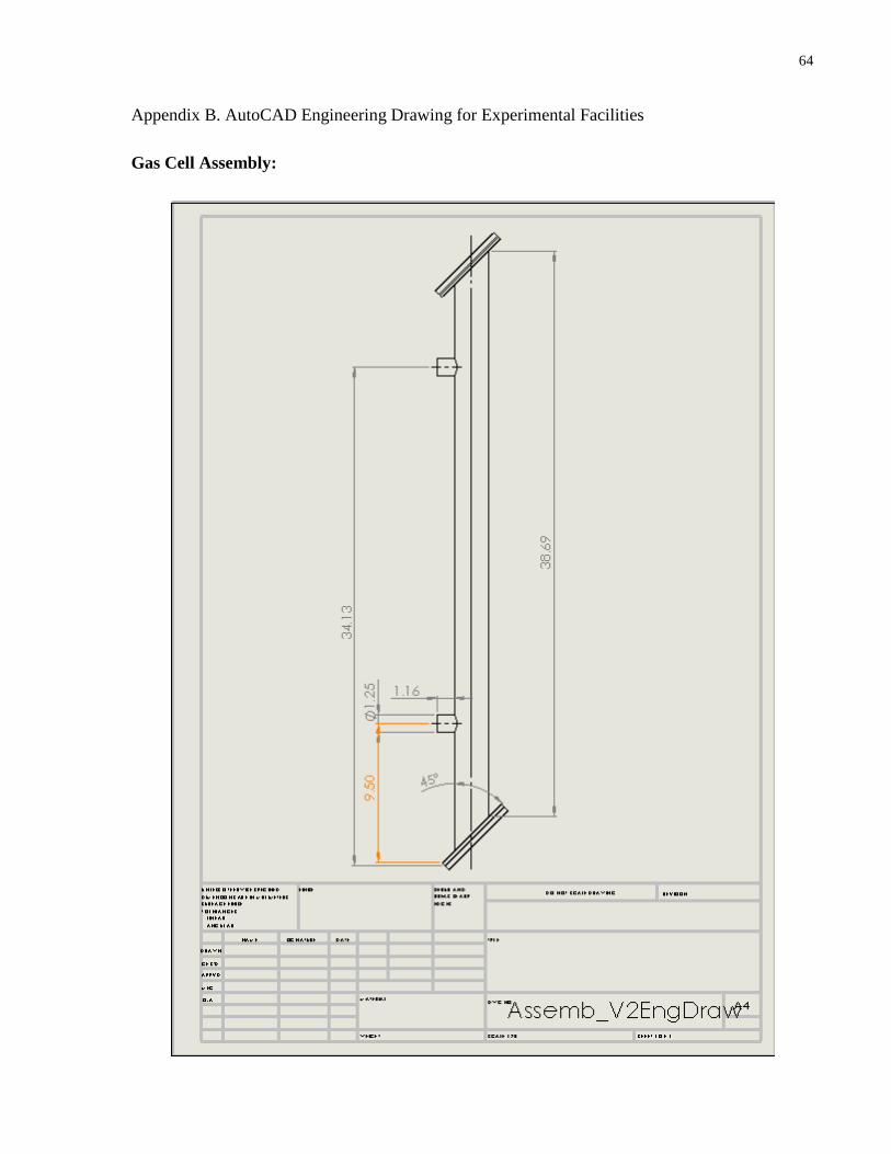
64

Appendix B. AutoCAD Engineering Drawing for Experimental Facilities

Gas Cell Assembly:

65

Front View of Purging Box:

66

Side-View of the Purging Box Shell:

67

Appendix C. MatLab Codes for Data Processing

Main Program: clc close all clear all %% For March 13th 14th tests different humidities with different references name0={'bg2', 'ref50_2', 'sig50_2','ref80_2','sig80_2','ref100_2','sig100_2','ref150_2','sig150_2','ref180_2','sig180_2','ref200_2', 'sig200_2','ref250_2','sig250_2','ref280_2','sig280_2','ref300_2', 'sig300_2',... 'ref350_2','sig350_2','ref380_2','sig380_2','ref400_2', 'sig400_2','ref450_2'};%,'sig450_2','ref480_2','sig480_2','ref550_2','sig550_ for k=1:length(name0) name{k}=name0{k}; end co='cbrkbgkkmgrgkmcbkrcybbyrkbyrk'; % Reading data and Averaging for k=1:length(name0) [Xave{k},Yave{k}]=xiaohuifun3(name{k},co(k)); end figure for k=[1 10 11] semilogy(Xave{k},Yave{k},co(k)); hold on end for k=3:2:length(name0) y{k-2}=-log((Yave{k}-Yave{1})./(Yave{k-1}-Yave{1})); % Subtraction] yy{k-2} = sgolayfilt(y{k-2},3,17); % SGolay Smooth rms_y(k-2)=sqrt(var(cell2mat(y(k-2)))); end rms_y=rms_y'; figure for k=[19 21 23 ] plot(Xave{1}./0.0303,y{k},co(k)); hold on end figure for k=[19 21 23 ] plot(Xave{1}./0.0303,yy{k},co(k)); hold on

68

end yy=cell2mat(yy); C=cell2mat(Yave); C=[Xave{1}./0.0303 C]; xlabel('wavenumber(cm-1)'); ylabel('Absorption'); A=[Xave{1}./0.0303 yy]; B=[Xave{1}./0.0303 y]; % for TTF filtering B=cell2mat(B); Y=cell2mat(y);

Functions: function [Xave, Yave]=xiaohuifun3(name,color); pq='July_4_diff_hum'; % pq='Apr_8_diff_hum'; if pq(end)~='\' pq=[pq '\']; end % f=dir([pq '*' name '*.csv']); f=dir([pq name '\*.csv']); n=length(f); X=[]; Y=[]; for k=1:n k; fname=[pq name '\' f(k).name] fdata.data=csvread(fname,1,0); z=size(fdata.data,1) z=304; % for 0.5-0.8THz scans X=[X,fdata.data(1:z,1)]; Y=[Y,fdata.data(1:z,4)]; % end Xave=mean(X,2); Yave=mean(Y,2); figure plot(Xave,Yave,color,'LineWidth',1.5); end